wasserstein generative adversarial networksproceedings.mlr.press/v70/arjovsky17a/arjovsky17a.pdf ·...

Wasserstein Generative Adversarial Networks

Martin Arjovsky 1 Soumith Chintala 2 Leon Bottou 1 2

AbstractWe introduce a new algorithm named WGAN,an alternative to traditional GAN training. Inthis new model, we show that we can improvethe stability of learning, get rid of problems likemode collapse, and provide meaningful learningcurves useful for debugging and hyperparametersearches. Furthermore, we show that the cor-responding optimization problem is sound, andprovide extensive theoretical work highlightingthe deep connections to different distances be-tween distributions.

1. IntroductionThe problem this paper is concerned with is that of unsu-pervised learning. Mainly, what does it mean to learn aprobability distribution? The classical answer to this is tolearn a probability density. This is often done by defininga parametric family of densities (Pθ)θ∈Rd and finding theone that maximized the likelihood on our data: if we havereal data examples {x(i)}mi=1, we would solve the problem

maxθ∈Rd

1

m

m∑i=1

logPθ(x(i))

If the real data distribution Pr admits a density and Pθ is thedistribution of the parametrized density Pθ, then, asymp-totically, this amounts to minimizing the Kullback-Leiblerdivergence KL(Pr‖Pθ).

For this to make sense, we need the model density Pθ toexist. This is not the case in the rather common situationwhere we are dealing with distributions supported by lowdimensional manifolds. It is then unlikely that the modelmanifold and the true distribution’s support have a non-negligible intersection (see (Arjovsky & Bottou, 2017)),and this means that the KL distance is not defined (or sim-ply infinite).

1Courant Institute of Mathematical Sciences, NY 2FacebookAI Research, NY. Correspondence to: Martin Arjovsky <[email protected]>.

Proceedings of the 34 th International Conference on MachineLearning, Sydney, Australia, PMLR 70, 2017. Copyright 2017by the author(s).

The typical remedy is to add a noise term to the model dis-tribution. This is why virtually all generative models de-scribed in the classical machine learning literature includea noise component. In the simplest case, one assumes aGaussian noise with relatively high bandwidth in order tocover all the examples. It is well known, for instance, thatin the case of image generation models, this noise degradesthe quality of the samples and makes them blurry. For ex-ample, we can see in the recent paper (Wu et al., 2016)that the optimal standard deviation of the noise added tothe model when maximizing likelihood is around 0.1 toeach pixel in a generated image, when the pixels were al-ready normalized to be in the range [0, 1]. This is a veryhigh amount of noise, so much that when papers report thesamples of their models, they don’t add the noise term onwhich they report likelihood numbers. In other words, theadded noise term is clearly incorrect for the problem, but isneeded to make the maximum likelihood approach work.

Rather than estimating the density of Pr which may not ex-ist, we can define a random variable Z with a fixed dis-tribution p(z) and pass it through a parametric functiongθ : Z → X (typically a neural network of some kind)that directly generates samples following a certain distribu-tion Pθ. By varying θ, we can change this distribution andmake it close to the real data distribution Pr. This is use-ful in two ways. First of all, unlike densities, this approachcan represent distributions confined to a low dimensionalmanifold. Second, the ability to easily generate samples isoften more useful than knowing the numerical value of thedensity (for example in image superresolution or semanticsegmentation when considering the conditional distributionof the output image given the input image). In general, itis computationally difficult to generate samples given anarbitrary high dimensional density (Neal, 2001).

Variational Auto-Encoders (VAEs) (Kingma & Welling,2013) and Generative Adversarial Networks (GANs)(Goodfellow et al., 2014) are well known examples of thisapproach. Because VAEs focus on the approximate likeli-hood of the examples, they share the limitation of the stan-dard models and need to fiddle with additional noise terms.GANs offer much more flexibility in the definition of theobjective function, including Jensen-Shannon (Goodfellowet al., 2014), and all f -divergences (Nowozin et al., 2016)as well as some exotic combinations (Huszar, 2015). On


the other hand, training GANs is well known for being del-icate and unstable, for reasons theoretically investigated in(Arjovsky & Bottou, 2017).

In this paper, we direct our attention on the various ways tomeasure how close the model distribution and the real dis-tribution are, or equivalently, on the various ways to definea distance or divergence ρ(Pθ,Pr). The most fundamen-tal difference between such distances is their impact on theconvergence of sequences of probability distributions. Asequence of distributions (Pt)t∈N converges if and only ifthere is a distribution P∞ such that ρ(Pt,P∞) tends to zero,something that depends on how exactly the distance ρ isdefined. Informally, a distance ρ induces a weaker topol-ogy when it makes it easier for a sequence of distributionto converge.1 Section 2 clarifies how popular probabilitydistances differ in that respect.

In order to optimize the parameter θ, it is of course desir-able to define our model distribution Pθ in a manner thatmakes the mapping θ 7→ Pθ continuous. Continuity meansthat when a sequence of parameters θt converges to θ, thedistributions Pθt also converge to Pθ. However, it is essen-tial to remember that the notion of the convergence of thedistributions Pθt depends on the way we compute the dis-tance between distributions. The weaker this distance, theeasier it is to define a continuous mapping from θ-space toPθ-space, since it’s easier for the distributions to converge.The main reason we care about the mapping θ 7→ Pθ to becontinuous is as follows. If ρ is our notion of distance be-tween two distributions, we would like to have a loss func-tion θ 7→ ρ(Pθ,Pr) that is continuous, and this is equivalentto having the mapping θ 7→ Pθ be continuous when usingthe distance between distributions ρ.

The contributions of this paper are:

• In Section 2, we provide a comprehensive theoreticalanalysis of how the Earth Mover (EM) distance be-haves in comparison to popular probability distancesand divergences used in the context of learning distri-butions.

• In Section 3, we define a form of GAN calledWasserstein-GAN that minimizes a reasonable and ef-ficient approximation of the EM distance, and we the-oretically show that the corresponding optimizationproblem is sound.

• In Section 4, we empirically show that WGANs curethe main training problems of GANs. In particular,training WGANs does not require maintaining a care-ful balance in training of the discriminator and the

1More exactly, the topology induced by ρ is weaker than thatinduced by ρ′ when the set of convergent sequences under ρ is asuperset of that under ρ′.

generator, does not require a careful design of the net-work architecture either, and also reduces the modedropping that is typical in GANs. One of the mostcompelling practical benefits of WGANs is the abilityto continuously estimate the EM distance by trainingthe discriminator to optimality. Because they correlatewell with the observed sample quality, plotting theselearning curves is very useful for debugging and hy-perparameter searches.

2. Different DistancesWe now introduce our notation. Let X be a compact metricset, say the space of images [0, 1]d, and let Σ denote theset of all the Borel subsets of X . Let Prob(X ) denote thespace of probability measures defined on X . We can nowdefine elementary distances and divergences between twodistributions Pr,Pg ∈ Prob(X ):

• The Total Variation (TV) distance

δ(Pr,Pg) = supA∈Σ|Pr(A)− Pg(A)| .

• The Kullback-Leibler (KL) divergence

KL(Pr‖Pg) =

∫log

(Pr(x)

Pg(x)

)Pr(x)dµ(x) ,

where both Pr and Pg are assumed to admit densitieswith respect to a same measure µ defined on X .2 TheKL divergence is famously assymetric and possiblyinfinite when there are points such that Pg(x) = 0and Pr(x) > 0.

• The Jensen-Shannon (JS) divergence

JS(Pr,Pg) = KL(Pr‖Pm) +KL(Pg‖Pm) ,

where Pm is the mixture (Pr + Pg)/2. This diver-gence is symmetrical and always defined because wecan choose µ = Pm.

• The Earth-Mover (EM) distance or Wasserstein-1

W (Pr,Pg) = infγ∈Π(Pr,Pg)

E(x,y)∼γ[‖x− y‖

], (1)

where Π(Pr,Pg) is the set of all joint distributionsγ(x, y) whose marginals are respectively Pr and Pg .Intuitively, γ(x, y) indicates how much “mass” mustbe transported from x to y in order to transform thedistributions Pr into the distribution Pg . The EM dis-tance then is the “cost” of the optimal transport plan.

2Recall that a probability distribution Pr ∈ Prob(X ) admitsa density Pr(x) with respect to µ, that is, ∀A ∈ Σ, Pr(A) =∫APr(x)dµ(x), if and only it is absolutely continuous with re-

spect to µ, that is, ∀A ∈ Σ, µ(A) = 0 ⇒ Pr(A) = 0 .


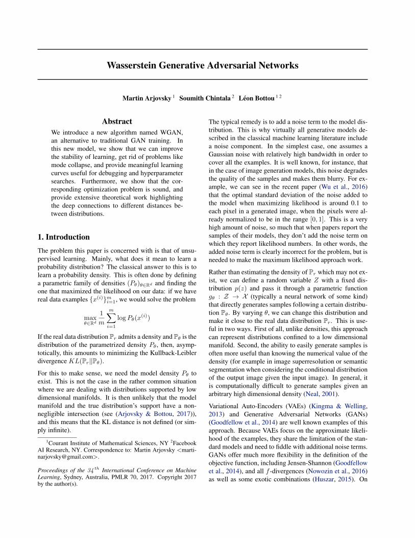
Figure 1: These plots show ρ(Pθ,P0) as a function of θ when ρ is the EM distance (left plot) or the JS divergence (right plot). The EMplot is continuous and provides a usable gradient everywhere. The JS plot is not continuous and does not provide a usable gradient.

The following example illustrates how apparently simplesequences of probability distributions converge under theEM distance but do not converge under the other distancesand divergences defined above.

Example 1 (Learning parallel lines). Let Z ∼ U [0, 1] theuniform distribution on the unit interval. Let P0 be the dis-tribution of (0, Z) ∈ R2 (a 0 on the x-axis and the randomvariable Z on the y-axis), uniform on a straight vertical linepassing through the origin. Now let gθ(z) = (θ, z) with θa single real parameter. It is easy to see that in this case,

• W (P0,Pθ) = |θ|,

• JS(P0,Pθ) =

{log 2 if θ 6= 0 ,

0 if θ = 0 ,

• KL(Pθ‖P0) = KL(P0‖Pθ) =

{+∞ if θ 6= 0 ,

0 if θ = 0 ,

• and δ(P0,Pθ) =

{1 if θ 6= 0 ,

0 if θ = 0 .

When θt → 0, the sequence (Pθt)t∈N converges to P0 un-der the EM distance, but does not converge at all undereither the JS, KL, reverse KL, or TV divergences. Figure 1illustrates this for the case of the EM and JS distances.

Example 1 gives a case where we can learn a probabilitydistribution over a low dimensional manifold by doing gra-dient descent on the EM distance. This cannot be done withthe other distances and divergences because the resultingloss function is not even continuous. Although this simpleexample features distributions with disjoint supports, thesame conclusion holds when the supports have a non emptyintersection contained in a set of measure zero. This hap-pens to be the case when two low dimensional manifoldsintersect in general position (Arjovsky & Bottou, 2017).

Since the Wasserstein distance is much weaker than the JS

distance,3 we can now ask whether W (Pr,Pθ) is a contin-uous loss function on θ under mild assumptions:Theorem 1. Let Pr be a fixed distribution over X . LetZ be a random variable (e.g Gaussian) over anotherspace Z . Let Pθ denote the distribution of gθ(Z) whereg : (z, θ) ∈ Z × Rd 7→ gθ(z) ∈ X . Then,

1. If g is continuous in θ, so is W (Pr,Pθ).

2. If g is locally Lipschitz and satisfies regularity as-sumption 1, then W (Pr,Pθ) is continuous every-where, and differentiable almost everywhere.

3. Statements 1-2 are false for the Jensen-Shannon di-vergence JS(Pr,Pθ) and all the KLs.

As a consequence, learning by minimizing the EM distancemakes sense (at least in theory) for neural networks:Corollary 1. Let gθ be any feedforward neural network4

parameterized by θ, and p(z) a prior over z such thatEz∼p(z)[‖z‖] < ∞ (e.g. Gaussian, uniform, etc.). Thenassumption 1 is satisfied and therefore W (Pr,Pθ) is con-tinuous everywhere and differentiable almost everywhere.

Both proofs are given in Appendix C.

All this indicates that EM is a much more sensible costfunction for our problem than at least the Jensen-Shannondivergence. The following theorem describes the relativestrength of the topologies induced by these distances anddivergences, with KL the strongest, followed by JS and TV,and EM the weakest.Theorem 2. Let P be a distribution on a compact space Xand (Pn)n∈N be a sequence of distributions on X . Then,considering all limits as n→∞,

3Appendix A explains to the mathematically inclined readerwhy this happens and how we arrived to the idea that Wassersteinis what we should really be optimizing.

4By a feedforward neural network we mean a function com-posed of affine transformations and componentwise Lipschitznonlinearities (such as the sigmoid, tanh, elu, softplus, etc). Asimilar but more technical proof is required for ReLUs.


1. The following statements are equivalent

• δ(Pn,P)→ 0 with δ the total variation distance.• JS(Pn,P)→ 0 with JS the Jensen-Shannon di-

vergence.

2. The following statements are equivalent

• W (Pn,P)→ 0.

• PnD−→ P where D−→ represents convergence in

distribution for random variables.

3. KL(Pn‖P) → 0 or KL(P‖Pn) → 0 imply the state-ments in (1).

4. The statements in (1) imply the statements in (2).

Proof. See Appendix C

This highlights the fact that the KL, JS, and TV distancesare not sensible cost functions when learning distributionssupported by low dimensional manifolds. However the EMdistance is sensible in that setup. This leads us to the nextsection where we introduce a practical approximation ofoptimizing the EM distance.

3. Wasserstein GANAgain, Theorem 2 points to the fact that W (Pr,Pθ) mighthave nicer properties when optimized than JS(Pr,Pθ).However, the infimum in (1) is highly intractable. On theother hand, the Kantorovich-Rubinstein duality (Villani,2009) tells us that

W (Pr,Pθ) = sup‖f‖L≤1

Ex∼Pr [f(x)]− Ex∼Pθ [f(x)] (2)

where the supremum is over all the 1-Lipschitz functionsf : X → R. Note that if we replace ‖f‖L ≤ 1 for‖f‖L ≤ K (consider K-Lipschitz for some constant K),then we end up with K ·W (Pr,Pg). Therefore, if we havea parameterized family of functions {fw}w∈W that are allK-Lipschitz for some K, we could consider solving theproblem

maxw∈W

Ex∼Pr [fw(x)]− Ez∼p(z)[fw(gθ(z)] (3)

and if the supremum in (2) is attained for some w ∈ W(a pretty strong assumption akin to what’s assumed whenproving consistency of an estimator), this process wouldyield a calculation of W (Pr,Pθ) up to a multiplicativeconstant. Furthermore, we could consider differentiat-ing W (Pr,Pθ) (again, up to a constant) by back-propingthrough equation (2) via estimating Ez∼p(z)[∇θfw(gθ(z))].While this is all intuition, we now prove that this process isprincipled under the optimality assumption.

Algorithm 1 WGAN, our proposed algorithm. All exper-iments in the paper used the default values α = 0.00005,c = 0.01, m = 64, ncritic = 5.Require: : α, the learning rate. c, the clipping parameter.

m, the batch size. ncritic, the number of iterations of thecritic per generator iteration.

Require: : w0, initial critic parameters. θ0, initial genera-tor’s parameters.

1: while θ has not converged do2: for t = 0, ..., ncritic do3: Sample {x(i)}mi=1 ∼ Pr a batch from the real data.4: Sample {z(i)}mi=1 ∼ p(z) a batch of priors.5: gw ← ∇w[ 1

m

∑mi=1 fw(x(i))

− 1m

∑mi=1 fw(gθ(z

(i)))]6: w ← w + α · RMSProp(w, gw)7: w ← clip(w,−c, c)8: end for9: Sample {z(i)}mi=1 ∼ p(z) a batch of prior samples.

10: gθ ← −∇θ 1m

∑mi=1 fw(gθ(z

(i)))11: θ ← θ − α · RMSProp(θ, gθ)12: end while

Theorem 3. Let Pr be any distribution. Let Pθ be the dis-tribution of gθ(Z) with Z a random variable with density pand gθ a function satisfying assumption 1. Then, there is asolution f : X → R to the problem

max‖f‖L≤1

Ex∼Pr [f(x)]− Ex∼Pθ [f(x)]

and we have

∇θW (Pr,Pθ) = −Ez∼p(z)[∇θf(gθ(z))]

when both terms are well-defined.

Proof. See Appendix C

Now comes the question of finding the function f thatsolves the maximization problem in equation (2). Toroughly approximate this, something that we can do istrain a neural network parameterized with weights w ly-ing in a compact space W and then backprop throughEz∼p(z)[∇θfw(gθ(z))], as we would do with a typicalGAN. Note that the fact thatW is compact implies that allthe functions fw will be K-Lipschitz for some K that onlydepends on W and not the individual weights, thereforeapproximating (2) up to an irrelevant scaling factor and thecapacity of the ‘critic’ fw. In order to have parametersw liein a compact space, something simple we can do is clampthe weights to a fixed box (say W = [−0.01, 0.01]l) aftereach gradient update. The Wasserstein Generative Adver-sarial Network (WGAN) procedure is described in Algo-rithm 1.


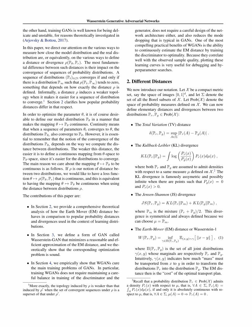
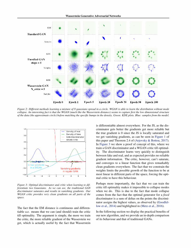
Figure 2: Different methods learning a mixture of 8 gaussians spread in a circle. WGAN is able to learn the distribution without modecollapse. An interesting fact is that the WGAN (much like the Wasserstein distance) seems to capture first the low dimensional structureof the data (the approximate circle) before matching the specific bumps in the density. Green: KDE plots. Blue: samples from the model.

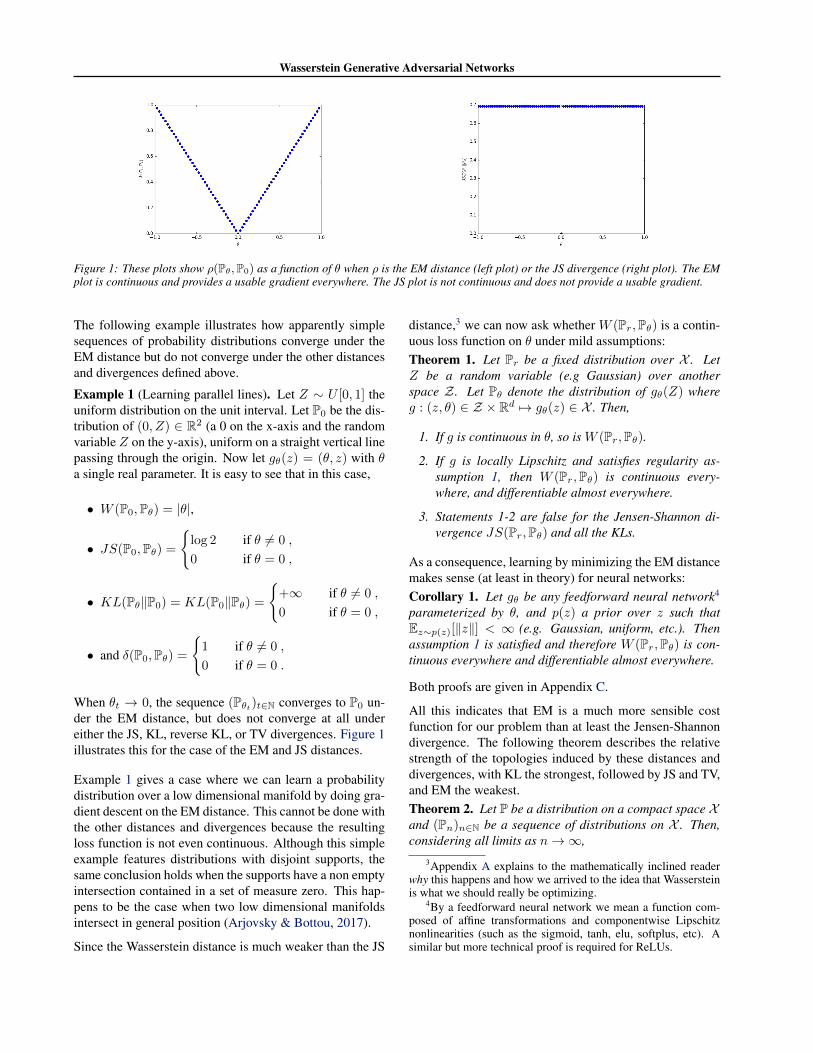
Figure 3: Optimal discriminator and critic when learning to dif-ferentiate two Gaussians. As we can see, the traditional GANdiscriminator saturates and results in vanishing gradients. OurWGAN critic provides very clean gradients on all parts of thespace.

The fact that the EM distance is continuous and differen-tiable a.e. means that we can (and should) train the critictill optimality. The argument is simple, the more we trainthe critic, the more reliable gradient of the Wasserstein weget, which is actually useful by the fact that Wasserstein

is differentiable almost everywhere. For the JS, as the dis-criminator gets better the gradients get more reliable butthe true gradient is 0 since the JS is locally saturated andwe get vanishing gradients, as can be seen in Figure 1 ofthis paper and Theorem 2.4 of (Arjovsky & Bottou, 2017).In Figure 3 we show a proof of concept of this, where wetrain a GAN discriminator and a WGAN critic till optimal-ity. The discriminator learns very quickly to distinguishbetween fake and real, and as expected provides no reliablegradient information. The critic, however, can’t saturate,and converges to a linear function that gives remarkablyclean gradients everywhere. The fact that we constrain theweights limits the possible growth of the function to be atmost linear in different parts of the space, forcing the opti-mal critic to have this behaviour.

Perhaps more importantly, the fact that we can train thecritic till optimality makes it impossible to collapse modeswhen we do. This is due to the fact that mode collapsecomes from the fact that the optimal generator for a fixeddiscriminator is a sum of deltas on the points the discrimi-nator assigns the highest values, as observed by (Goodfel-low et al., 2014) and highlighted in (Metz et al., 2016).

In the following section we display the practical benefits ofour new algorithm, and we provide an in-depth comparisonof its behaviour and that of traditional GANs.


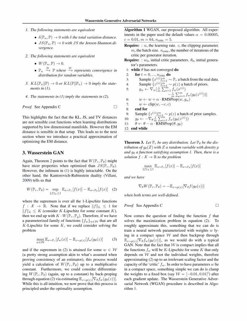
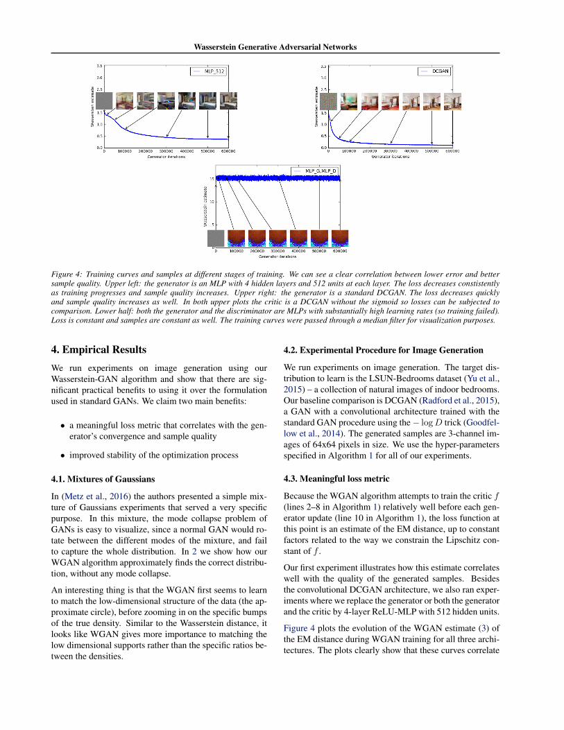
Figure 4: Training curves and samples at different stages of training. We can see a clear correlation between lower error and bettersample quality. Upper left: the generator is an MLP with 4 hidden layers and 512 units at each layer. The loss decreases constistentlyas training progresses and sample quality increases. Upper right: the generator is a standard DCGAN. The loss decreases quicklyand sample quality increases as well. In both upper plots the critic is a DCGAN without the sigmoid so losses can be subjected tocomparison. Lower half: both the generator and the discriminator are MLPs with substantially high learning rates (so training failed).Loss is constant and samples are constant as well. The training curves were passed through a median filter for visualization purposes.

4. Empirical ResultsWe run experiments on image generation using ourWasserstein-GAN algorithm and show that there are sig-nificant practical benefits to using it over the formulationused in standard GANs. We claim two main benefits:

• a meaningful loss metric that correlates with the gen-erator’s convergence and sample quality

• improved stability of the optimization process

4.1. Mixtures of Gaussians

In (Metz et al., 2016) the authors presented a simple mix-ture of Gaussians experiments that served a very specificpurpose. In this mixture, the mode collapse problem ofGANs is easy to visualize, since a normal GAN would ro-tate between the different modes of the mixture, and failto capture the whole distribution. In 2 we show how ourWGAN algorithm approximately finds the correct distribu-tion, without any mode collapse.

An interesting thing is that the WGAN first seems to learnto match the low-dimensional structure of the data (the ap-proximate circle), before zooming in on the specific bumpsof the true density. Similar to the Wasserstein distance, itlooks like WGAN gives more importance to matching thelow dimensional supports rather than the specific ratios be-tween the densities.

4.2. Experimental Procedure for Image Generation

We run experiments on image generation. The target dis-tribution to learn is the LSUN-Bedrooms dataset (Yu et al.,2015) – a collection of natural images of indoor bedrooms.Our baseline comparison is DCGAN (Radford et al., 2015),a GAN with a convolutional architecture trained with thestandard GAN procedure using the− logD trick (Goodfel-low et al., 2014). The generated samples are 3-channel im-ages of 64x64 pixels in size. We use the hyper-parametersspecified in Algorithm 1 for all of our experiments.

4.3. Meaningful loss metric

Because the WGAN algorithm attempts to train the critic f(lines 2–8 in Algorithm 1) relatively well before each gen-erator update (line 10 in Algorithm 1), the loss function atthis point is an estimate of the EM distance, up to constantfactors related to the way we constrain the Lipschitz con-stant of f .

Our first experiment illustrates how this estimate correlateswell with the quality of the generated samples. Besidesthe convolutional DCGAN architecture, we also ran exper-iments where we replace the generator or both the generatorand the critic by 4-layer ReLU-MLP with 512 hidden units.

Figure 4 plots the evolution of the WGAN estimate (3) ofthe EM distance during WGAN training for all three archi-tectures. The plots clearly show that these curves correlate


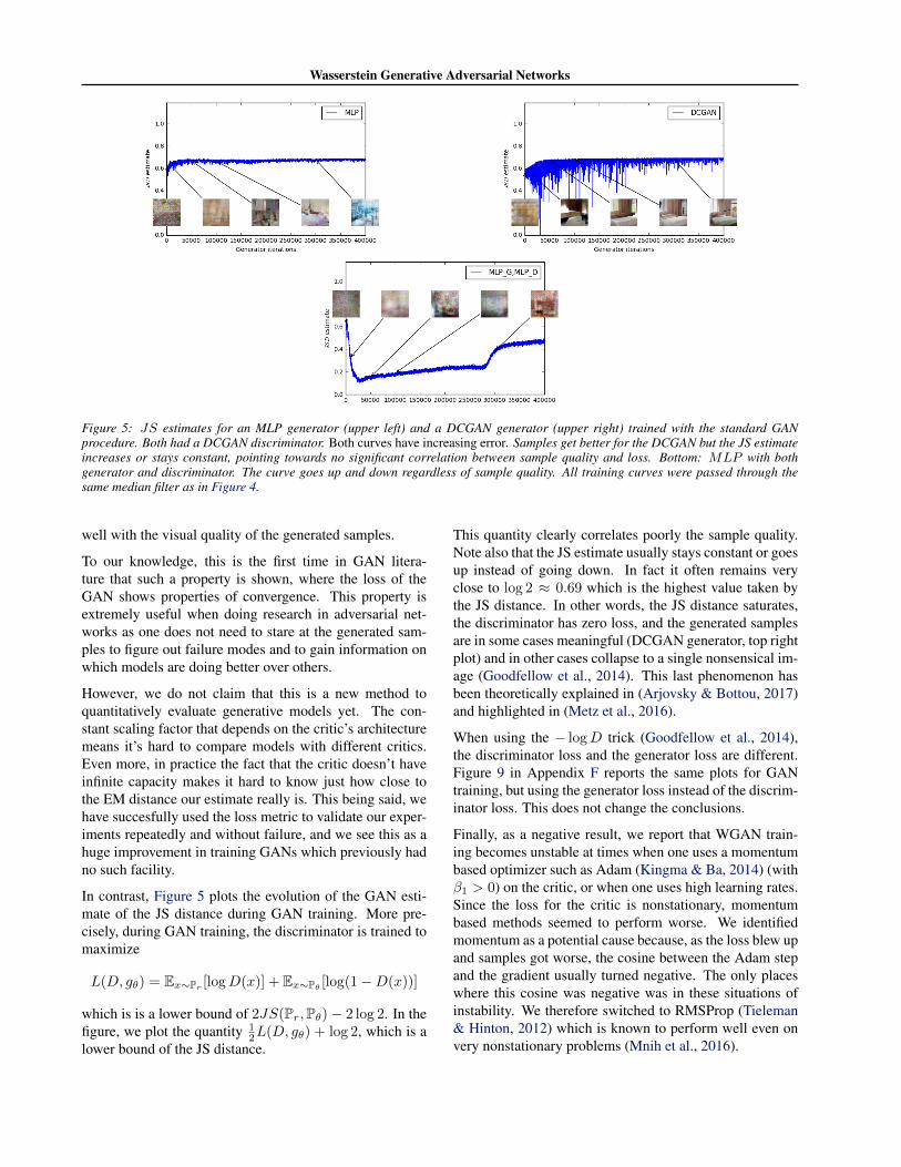
Figure 5: JS estimates for an MLP generator (upper left) and a DCGAN generator (upper right) trained with the standard GANprocedure. Both had a DCGAN discriminator. Both curves have increasing error. Samples get better for the DCGAN but the JS estimateincreases or stays constant, pointing towards no significant correlation between sample quality and loss. Bottom: MLP with bothgenerator and discriminator. The curve goes up and down regardless of sample quality. All training curves were passed through thesame median filter as in Figure 4.

well with the visual quality of the generated samples.

To our knowledge, this is the first time in GAN litera-ture that such a property is shown, where the loss of theGAN shows properties of convergence. This property isextremely useful when doing research in adversarial net-works as one does not need to stare at the generated sam-ples to figure out failure modes and to gain information onwhich models are doing better over others.

However, we do not claim that this is a new method toquantitatively evaluate generative models yet. The con-stant scaling factor that depends on the critic’s architecturemeans it’s hard to compare models with different critics.Even more, in practice the fact that the critic doesn’t haveinfinite capacity makes it hard to know just how close tothe EM distance our estimate really is. This being said, wehave succesfully used the loss metric to validate our exper-iments repeatedly and without failure, and we see this as ahuge improvement in training GANs which previously hadno such facility.

In contrast, Figure 5 plots the evolution of the GAN esti-mate of the JS distance during GAN training. More pre-cisely, during GAN training, the discriminator is trained tomaximize

L(D, gθ) = Ex∼Pr [logD(x)] + Ex∼Pθ [log(1−D(x))]

which is is a lower bound of 2JS(Pr,Pθ)− 2 log 2. In thefigure, we plot the quantity 1

2L(D, gθ) + log 2, which is alower bound of the JS distance.

This quantity clearly correlates poorly the sample quality.Note also that the JS estimate usually stays constant or goesup instead of going down. In fact it often remains veryclose to log 2 ≈ 0.69 which is the highest value taken bythe JS distance. In other words, the JS distance saturates,the discriminator has zero loss, and the generated samplesare in some cases meaningful (DCGAN generator, top rightplot) and in other cases collapse to a single nonsensical im-age (Goodfellow et al., 2014). This last phenomenon hasbeen theoretically explained in (Arjovsky & Bottou, 2017)and highlighted in (Metz et al., 2016).

When using the − logD trick (Goodfellow et al., 2014),the discriminator loss and the generator loss are different.Figure 9 in Appendix F reports the same plots for GANtraining, but using the generator loss instead of the discrim-inator loss. This does not change the conclusions.

Finally, as a negative result, we report that WGAN train-ing becomes unstable at times when one uses a momentumbased optimizer such as Adam (Kingma & Ba, 2014) (withβ1 > 0) on the critic, or when one uses high learning rates.Since the loss for the critic is nonstationary, momentumbased methods seemed to perform worse. We identifiedmomentum as a potential cause because, as the loss blew upand samples got worse, the cosine between the Adam stepand the gradient usually turned negative. The only placeswhere this cosine was negative was in these situations ofinstability. We therefore switched to RMSProp (Tieleman& Hinton, 2012) which is known to perform well even onvery nonstationary problems (Mnih et al., 2016).


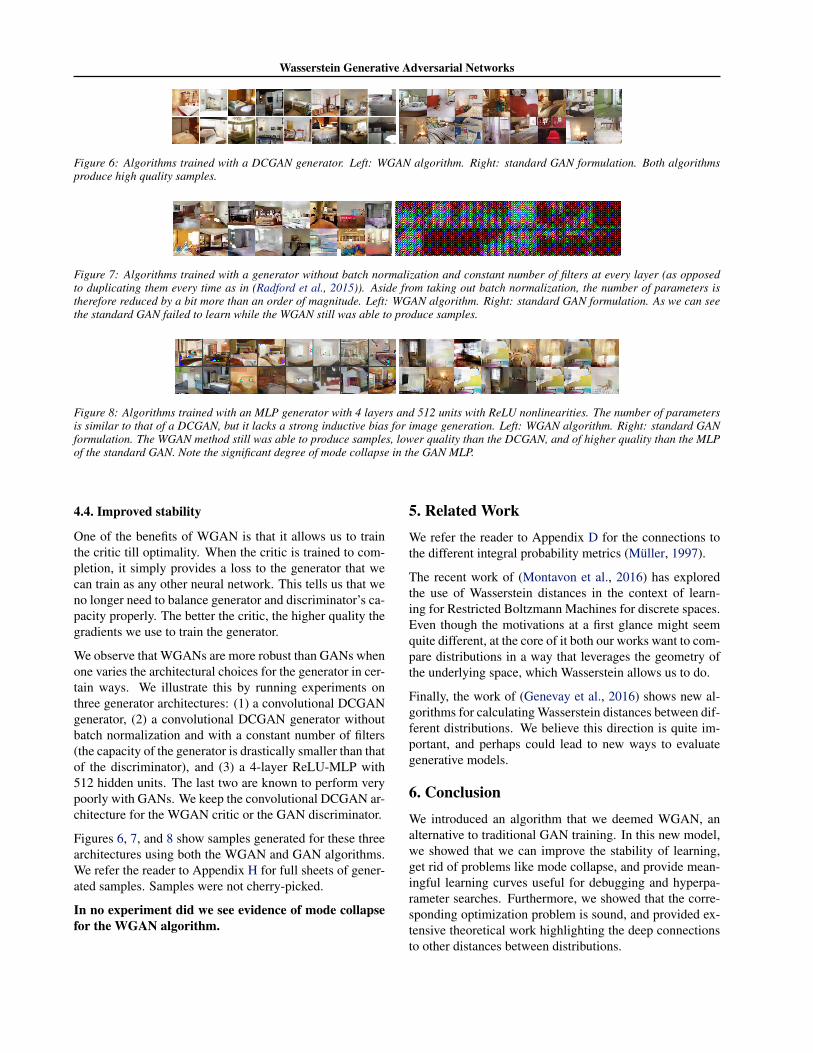
Figure 6: Algorithms trained with a DCGAN generator. Left: WGAN algorithm. Right: standard GAN formulation. Both algorithmsproduce high quality samples.

Figure 7: Algorithms trained with a generator without batch normalization and constant number of filters at every layer (as opposedto duplicating them every time as in (Radford et al., 2015)). Aside from taking out batch normalization, the number of parameters istherefore reduced by a bit more than an order of magnitude. Left: WGAN algorithm. Right: standard GAN formulation. As we can seethe standard GAN failed to learn while the WGAN still was able to produce samples.

Figure 8: Algorithms trained with an MLP generator with 4 layers and 512 units with ReLU nonlinearities. The number of parametersis similar to that of a DCGAN, but it lacks a strong inductive bias for image generation. Left: WGAN algorithm. Right: standard GANformulation. The WGAN method still was able to produce samples, lower quality than the DCGAN, and of higher quality than the MLPof the standard GAN. Note the significant degree of mode collapse in the GAN MLP.

4.4. Improved stability

One of the benefits of WGAN is that it allows us to trainthe critic till optimality. When the critic is trained to com-pletion, it simply provides a loss to the generator that wecan train as any other neural network. This tells us that weno longer need to balance generator and discriminator’s ca-pacity properly. The better the critic, the higher quality thegradients we use to train the generator.

We observe that WGANs are more robust than GANs whenone varies the architectural choices for the generator in cer-tain ways. We illustrate this by running experiments onthree generator architectures: (1) a convolutional DCGANgenerator, (2) a convolutional DCGAN generator withoutbatch normalization and with a constant number of filters(the capacity of the generator is drastically smaller than thatof the discriminator), and (3) a 4-layer ReLU-MLP with512 hidden units. The last two are known to perform verypoorly with GANs. We keep the convolutional DCGAN ar-chitecture for the WGAN critic or the GAN discriminator.

Figures 6, 7, and 8 show samples generated for these threearchitectures using both the WGAN and GAN algorithms.We refer the reader to Appendix H for full sheets of gener-ated samples. Samples were not cherry-picked.

In no experiment did we see evidence of mode collapsefor the WGAN algorithm.

5. Related WorkWe refer the reader to Appendix D for the connections tothe different integral probability metrics (Muller, 1997).

The recent work of (Montavon et al., 2016) has exploredthe use of Wasserstein distances in the context of learn-ing for Restricted Boltzmann Machines for discrete spaces.Even though the motivations at a first glance might seemquite different, at the core of it both our works want to com-pare distributions in a way that leverages the geometry ofthe underlying space, which Wasserstein allows us to do.

Finally, the work of (Genevay et al., 2016) shows new al-gorithms for calculating Wasserstein distances between dif-ferent distributions. We believe this direction is quite im-portant, and perhaps could lead to new ways to evaluategenerative models.

6. ConclusionWe introduced an algorithm that we deemed WGAN, analternative to traditional GAN training. In this new model,we showed that we can improve the stability of learning,get rid of problems like mode collapse, and provide mean-ingful learning curves useful for debugging and hyperpa-rameter searches. Furthermore, we showed that the corre-sponding optimization problem is sound, and provided ex-tensive theoretical work highlighting the deep connectionsto other distances between distributions.


AcknowledgmentsWe would like to thank Mohamed Ishmael Belghazi, EmilyDenton, Ian Goodfellow, Ishaan Gulrajani, Alex Lamb,David Lopez-Paz, Eric Martin, musyoku, Maxime Oquab,Aditya Ramesh, Ronan Riochet, Uri Shalit, Pablo Sprech-mann, Arthur Szlam, Ruohan Wang, for helpful commentsand advice.

ReferencesArjovsky, Martin and Bottou, Leon. Towards principled

methods for training generative adversarial networks. InInternational Conference on Learning Representations,2017.

Dziugaite, Gintare Karolina, Roy, Daniel M., and Ghahra-mani, Zoubin. Training generative neural networksvia maximum mean discrepancy optimization. CoRR,abs/1505.03906, 2015.

Genevay, Aude, Cuturi, Marco, Peyre, Gabriel, and Bach,Francis. Stochastic optimization for large-scale optimaltransport. In Lee, D. D., Sugiyama, M., Luxburg, U. V.,Guyon, I., and Garnett, R. (eds.), Advances in Neural In-formation Processing Systems 29, pp. 3440–3448. Cur-ran Associates, Inc., 2016.

Goodfellow, Ian J., Pouget-Abadie, Jean, Mirza, Mehdi,Xu, Bing, Warde-Farley, David, Ozair, Sherjil,Courville, Aaron, and Bengio, Yoshua. Generative ad-versarial nets. In Advances in Neural Information Pro-cessing Systems 27, pp. 2672–2680. Curran Associates,Inc., 2014.

Gretton, Arthur, Borgwardt, Karsten M., Rasch, Malte J.,Scholkopf, Bernhard, and Smola, Alexander. A ker-nel two-sample test. J. Mach. Learn. Res., 13:723–773,2012. ISSN 1532-4435.

Huszar, Ferenc. How (not) to train your generative model:Scheduled sampling, likelihood, adversary? CoRR,abs/1511.05101, 2015.

Kakutani, Shizuo. Concrete representation of abstract (m)-spaces (a characterization of the space of continuousfunctions). Annals of Mathematics, 42(4):994–1024,1941.

Kingma, Diederik P. and Ba, Jimmy. Adam: A method forstochastic optimization. CoRR, abs/1412.6980, 2014.

Kingma, Diederik P. and Welling, Max. Auto-encodingvariational bayes. CoRR, abs/1312.6114, 2013.

Li, Yujia, Swersky, Kevin, and Zemel, Rich. Generativemoment matching networks. In Proceedings of the 32nd

International Conference on Machine Learning (ICML-15), pp. 1718–1727. JMLR Workshop and ConferenceProceedings, 2015.

Metz, Luke, Poole, Ben, Pfau, David, and Sohl-Dickstein,Jascha. Unrolled generative adversarial networks. Corr,abs/1611.02163, 2016.

Milgrom, Paul and Segal, Ilya. Envelope theorems for ar-bitrary choice sets. Econometrica, 70(2):583–601, 2002.ISSN 1468-0262.

Mnih, Volodymyr, Badia, Adria Puigdomenech, Mirza,Mehdi, Graves, Alex, Lillicrap, Timothy P., Harley, Tim,Silver, David, and Kavukcuoglu, Koray. Asynchronousmethods for deep reinforcement learning. In Proceed-ings of the 33nd International Conference on MachineLearning, ICML 2016, New York City, NY, USA, June19-24, 2016, pp. 1928–1937, 2016.

Montavon, Gregoire, Muller, Klaus-Robert, and Cuturi,Marco. Wasserstein training of restricted boltzmann ma-chines. In Lee, D. D., Sugiyama, M., Luxburg, U. V.,Guyon, I., and Garnett, R. (eds.), Advances in Neural In-formation Processing Systems 29, pp. 3718–3726. Cur-ran Associates, Inc., 2016.

Muller, Alfred. Integral probability metrics and their gen-erating classes of functions. Advances in Applied Prob-ability, 29(2):429–443, 1997.

Neal, Radford M. Annealed importance sampling. Statis-tics and Computing, 11(2):125–139, April 2001. ISSN0960-3174.

Nowozin, Sebastian, Cseke, Botond, and Tomioka, Ryota.f-gan: Training generative neural samplers using varia-tional divergence minimization. pp. 271–279, 2016.

Radford, Alec, Metz, Luke, and Chintala, Soumith. Unsu-pervised representation learning with deep convolutionalgenerative adversarial networks. CoRR, abs/1511.06434,2015.

Ramdas, Aaditya, Reddi, Sashank J., Poczos, Barn-abas, Singh, Aarti, and Wasserman, Larry. Onthe high-dimensional power of linear-time kernel two-sample testing under mean-difference alternatives. Corr,abs/1411.6314, 2014.

Sutherland, Dougal J, Tung, Hsiao-Yu, Strathmann, Heiko,De, Soumyajit, Ramdas, Aaditya, Smola, Alex, andGretton, Arthur. Generative models and model criticismvia optimized maximum mean discrepancy. In Interna-tional Conference on Learning Representations, 2017.


Tieleman, T. and Hinton, G. Lecture 6.5—RmsProp: Di-vide the gradient by a running average of its recent mag-nitude. COURSERA: Neural Networks for MachineLearning, 2012.

Villani, Cedric. Optimal Transport: Old and New.Grundlehren der mathematischen Wissenschaften.Springer, Berlin, 2009.

Wu, Yuhuai, Burda, Yuri, Salakhutdinov, Ruslan, andGrosse, Roger B. On the quantitative analy-sis of decoder-based generative models. CoRR,abs/1611.04273, 2016.

Yu, Fisher, Zhang, Yinda, Song, Shuran, Seff, Ari, andXiao, Jianxiong. LSUN: Construction of a large-scaleimage dataset using deep learning with humans in theloop. Corr, abs/1506.03365, 2015.

Zhao, Junbo, Mathieu, Michael, and LeCun, Yann.Energy-based generative adversarial network. Corr,abs/1609.03126, 2016.

wasserstein generative adversarial networksproceedings.mlr.press/v70/arjovsky17a/arjovsky17a.pdf ·...

Documents