voting with bidirectional elimination - economics · voting with bidirectional elimination matthew...

Voting with Bidirectional Elimination

Matthew S. Cook

Economics Department

Stanford University

March, 2011

Advisor:

Jonathan Levin

Abstract

Two important criteria for judging the quality of a voting algorithm are strategy-proofness and

Condorcet efficiency. While, according to the Gibbard-Satterthwaite theorem, we can expect no

voting mechanism to be fully strategy proof, many Condorcet methods are quite susceptible to

compromising, burying, and bullet voting. In this paper I propose a new algorithm which I call

“Bidirectional Elimination,” a composite of Instant Runoff Voting and the Coombs Method,

which offers the benefit of greater resistance to tactical voting while nearly always electing the

Condorcet winner when one exists. A program was used to test IRV, the Coombs Method, and

Bidirectional Elimination on tens of billions of social preferences profiles in combinations of up

to ten voters and ten candidates. I offer mathematical proofs that this new algorithm meets the

Condorcet criterion for up to 4 voters and N candidates, or M voters and up to 3 candidates;

beyond this, results from the program show that Bidirectional Elimination offers a significant

advantage over both IRV and Coombs in approaching Condorcet efficiency.

Key Words

Voting, tactical voting, Condorcet criterion, instant runoff voting, Coombs Method.

Acknowledgments I am grateful to Jonathan Levin for his instructive insights, engaging discussions, and thoughtful

guidance. A special thanks to Jaehyun Park for lending his world class coding talents in creating

the program I used to test tens of billions of samples. Discussions with Jonathan Zhang were

particularly enlightening: It was during conversation with him that the concept of Bidirectional

Elimination was born. Jon also independently created his own proof of Condorcet efficiency for

the [3 candidates, M voters] case. Tyler Mullen showed me a set of conditions under which my

algorithm would not elect the Condorcet winner. This led me to design the specifications for the

program Jaehyun coded. Thanks to the four of you for your support of this stimulating project.

Finally, thanks to Malcolm Clare for fascinating discussions related to social choice and politics.

I admire you as a philosopher, Professor Clare.

2

1. Introduction

For decades, the Academy of Motion Picture Arts and Sciences used a plurality vote to

determine Best Picture: Over five thousand voters would submit a single vote among just a few

nominees, and the movie receiving the most votes would win. In 2010, the Academy replaced

plurality voting with a new system called Instant Runoff Voting (IRV). Instead of submitting a

single choice, voters were asked to submit a preferential ranking of ten nominees. After all

ballots were cast, the mechanism would systematically eliminate candidates with the fewest first-

place votes until only the winner remained.

IRV offered several advantages over a simple plurality vote. The plurality mechanism

could have easily elected candidates many voters strongly disliked, and it also allowed for the

spoiler effect—the negative effect a weaker candidate has over a stronger candidate by stealing

away votes. To compensate for the spoiler effect, voters in the plurality elections were able to

strategize by failing to report actual first choices; voters could compromise by voting for the

candidate they thought realistically had the best chance of winning. Instant Runoff Voting

eliminated the spoiler effect and reduced the chance of electing candidates whom a majority

disliked.

In his February 15, 2010 article for The New Yorker, Hendrik Hertzberg explains the

effects of IRV in the context of that year’s Academy Awards:

“This scheme, [known as] instant-runoff voting, doesn’t necessarily get you the movie (or

the candidate) with the most committed supporters, but it does get you a winner that a majority

can at least countenance. It favors consensus. Now here’s why it may also favor The Hurt Locker.

A lot of people like Avatar, obviously, but a lot don’t—too cold, too formulaic, too computerized,

too derivative. . . . Avatar is polarizing. So is James Cameron. He may have fattened the bank

accounts of a sizable bloc of Academy members—some three thousand people drew Avatar

paychecks—but that doesn’t mean that they all long to recrown him king of the world. . . . These

factors could push Avatar toward the bottom of many a ranked-choice ballot.

On the other hand, few people who have seen The Hurt Locker—a real Iraq War story,

not a sci-fi allegory—actively dislike it, and many profoundly admire it. Its underlying ethos is

that war is hell, but it does not demonize the soldiers it portrays, whose job is to defuse bombs, not

drop them. Even Republicans (and there are a few in Hollywood) think it’s good. It will likely be

the second or third preference of voters whose first choice is one of the other ‘small’ films that

have been nominated.”

Like any process, voting requires a specific design. Designing a just voting system might

seem trivial: Why shouldn’t voters just state whom they wish to elect, and why shouldn’t the

system simply maximize voter utility in a fair manner? But there are problems associated with

both steps. According to Allan Gibbard and Mark Satterthwaite, no voting mechanism is fully

strategy proof, and according to Arrow, no voting mechanism meets all reasonable criteria of

fairness. A theoretical framework must be constructed to evaluate methods of aggregating

individual interests into a collective decision. This theoretical framework, dating back to the

work of French philosopher and mathematician Marquis de Condorcet, is called social choice

theory.

Within this framework, criteria exist for evaluating the justness of a voting mechanism.

The purpose of this paper is to define important criteria, explain their importance, and evaluate a

new voting mechanism using these criteria. The mechanism I will analyze is called Bidirectional

Elimination and is conducted in a manner similar to IRV. The criteria I will use are the

Condorcet criterion and strategy proofness. I will primarily analyze the mechanism based on the

3

Condorcet criterion, using mathematical proofs and experimental data from computer

simulations. I will discuss strategy proofness less, but recommend an experimental methodology

one could use for a rigorous analysis.

The paper is organized as follows. Section 2 reviews criteria, background, terminology,

and theorems related to social choice theory that are necessary for analyzing a voting

mechanism. Section 3 dissects Instant Runoff Voting, the Coombs Method, and Condorcet

Methods. Section 4 introduces Bidirectional Elimination, runs the algorithm step by step on a

given set of preferences, and analyzes based on certain criteria presented in section 2. Section 5

offers logic proofs related to Condorcet efficiency. Section 6 presents and analyzes experimental

results from a computer simulation. Section 7 offers concluding remarks.

Results from the computer simulation show that Bidirectional Elimination does not meet

the Condorcet criterion, but comes very close. Given the susceptibility of most Condorcet

methods to tactical voting, and given that failure to elect the Condorcet winner occurs less than

.6% of the time for up to 10 voters and 10 candidates using Bidirectional Elimination, I find that

this new algorithm may offer a significant advantage over Condorcet methods, and certainly a

strict advantage over Instant Runoff Voting and over the similar Coombs Method.

2. Background and Terminology

The first key term is Condorcet winner. The Condorcet winner is the candidate who,

when paired against any other individual candidate, will always capture a majority vote. A voting

method that always elects the Condorcet winner when one exists is called Condorcet efficient, or

is said to meet the Condorcet criterion. The Condorcet loser is one who always loses such

pairwise runoffs. A system that never elects the Condorcet loser is said to meet the Condorcet

loser criterion. A Condorcet method is a mechanism that will always elect the Condorcet winner.

A Condorcet winner does not always exist. Sometimes there will be a tie, or a cycle; the latter is

an example of Condorcet’s paradox. This occurs when, for example, three voters have

preferences (A>B>C), (B>C>A), and (C>A>B); in this case, the group chooses A over B, B over

C, and C over A, and there is no clear winner.

A second criterion for evaluating voting systems is strategy proofness. A voting system is

said to be strategy proof if, given full information over everyone else’s preferences, no individual

could ever improve his outcome by misreporting his own preferences. Such misreporting is

called tactical voting. According to the Gibbard-Satterthwaite theorem, no preferential voting

system is fully strategy proof.

Various types of tactical voting can occur. The first is called push-over voting, in which a

voter ranks a weak alternative higher, but not in the hopes of getting that alternative elected. The

second is called compromising, which occurs when voters dishonestly rank an alternative higher

than their true alternative in hopes of getting it elected. The third strategy, called burying, occurs

when a voter dishonestly ranks a candidate lower in hopes of seeing it defeated. The last form is

called bullet voting, which means voting for only one candidate in a preferential system when

submitting a list of ranked preferences is an option.

Susceptibility to strategic voting occurs when a voting method fails certain criteria.

Among them is the monotonicity criterion, which states that a candidate X must not be harmed—

that is, changed from being a winner to a loser—if X is raised on some ballots without changing

the orders of the other candidates. Conversely, the later-no-harm criterion states that giving a

more positive ranking, or simple an additional ranking, to a less preferred candidate must not

cause a more preferred candidate to lose.

4

Arrow’s impossibility theorem states that given at least three candidates, no preferential

voting system can meet all of the following reasonable criteria of fairness. (1) Unrestricted

domain: All permutations of voter preferences are allowed. (2) Non-dictatorship: No single voter

determines the outcome of the election. (3) Pareto-efficiency: No improvements can be made

without making another voter worse off. (4) Independence of irrelevant alternatives: An election

between candidates X and Y depends only on preferences between X and Y (changing the order

between X and Z would not affect the outcome between X and Y).

3. Relevant Voting Methods

Instant Runoff Voting

Instant Runoff Voting is a system using ranked preferences to elect a single winner. The

procedure works as follows. Voters submit ranked preferences, and the candidate with the fewest

first choice votes is systematically eliminated until only the winner remains. In some cases,

candidates will be tied for the position of “fewest first choice votes.” If this happens, special

tiebreaker rules must be constructed.

IRV satisfies the later-no-harm criterion and the Condorcet loser criterion but fails

monotonicity, independence of irrelevant alternatives, and the Condorcet criterion.

IRV is susceptible to push-over voting.

Coombs Method

The Coombs Method is a system similar to IRV using ranked preferences to elect a single

winner. Instead of systematically eliminating the candidate with the fewest first choice votes,

Coombs systematically eliminates the candidate with the most last choice votes until one

remains. Similarly, a special tiebreaker must be devised to deal with cases in which candidates

are tied for the position of “most last choice votes.”

The Coombs Method satisfies the Condorcet loser criterion but fails monotonicity,

independence of irrelevant alternatives, and the Condorcet criterion.

The Coombs Method is susceptible to compromising and burying.

Condorcet Methods

Condorcet methods, methods that will always elect the Condorcet winner, include

Copeland’s method, the Kemeny-Young Method, Minimax, Nanson’s method, ranked pairs, and

the Schulze method. No Condorcet method satisfies the later-no-harm criterion or independence

of irrelevant alternatives. The methods vary in monotonicity.

Condorcet methods are generally quite susceptible to tactical voting, in particular

compromising, burying, and bullet voting.

4. Bidirectional Elimination

I now propose a new voting mechanism using ranked preferences. I call this new

mechanism “Bidirectional Elimination,” as it is a hybrid of both Instant Runoff Voting and the

Coombs Method. The algorithm works as follows.

5

Note: The tiebreaker procedure described in stages 1 and 2 is important in preventing

premature elimination of the Condorcet winner.

The Bidirectional Elimination Algorithm

Stage 1: Use regular IRV to elect potential winner X. If in any round of elimination two

or more candidates share the least number of first choice votes, a special tiebreaker is performed.

To perform the tiebreaker, create a set of “potential losers” consisting of all candidates sharing

the least number of first choice votes in the leftmost column. Then move to the next column to

the right and reiterate this form of IRV among potential losers only, possibly narrowing the set of

potential losers, until one is eliminated; then continue with regular IRV. If potential losers are

ever tied in the rightmost column containing any potential losers, all potential losers are

eliminated at once. Under certain tiebreaker conditions, no winner will be elected; all candidates

are eliminated.

Stage 2: Use the Coombs Method to elect a potential winner Y. If in any round of

elimination two or more candidates share the highest number of last choice votes, a special

tiebreaker is performed. To perform the tiebreaker, create a set of “potential losers” consisting of

all the candidates sharing the highest number of last choice votes in the rightmost column. Then

move to the next column to the left and reiterate this form of the Coombs Method among

potential losers only, possibly narrowing the set of potential losers, until one is eliminated; then

continue with the regular Coombs Method. If potential losers are ever tied in the leftmost column

containing any potential losers, all potential losers are eliminated at once. Under certain

tiebreaker conditions, no winner will be elected; all candidates are eliminated.

Stage 3: If X and Y are the same candidate, X=Y is the winner; if X and Y are different

candidates, a simple pairwise runoff between X and Y determines the winner; if only one of the

stages elects a potential winner, the potential winner is the final winner; if neither former stage

elects a potential winner, then there is no final winner.

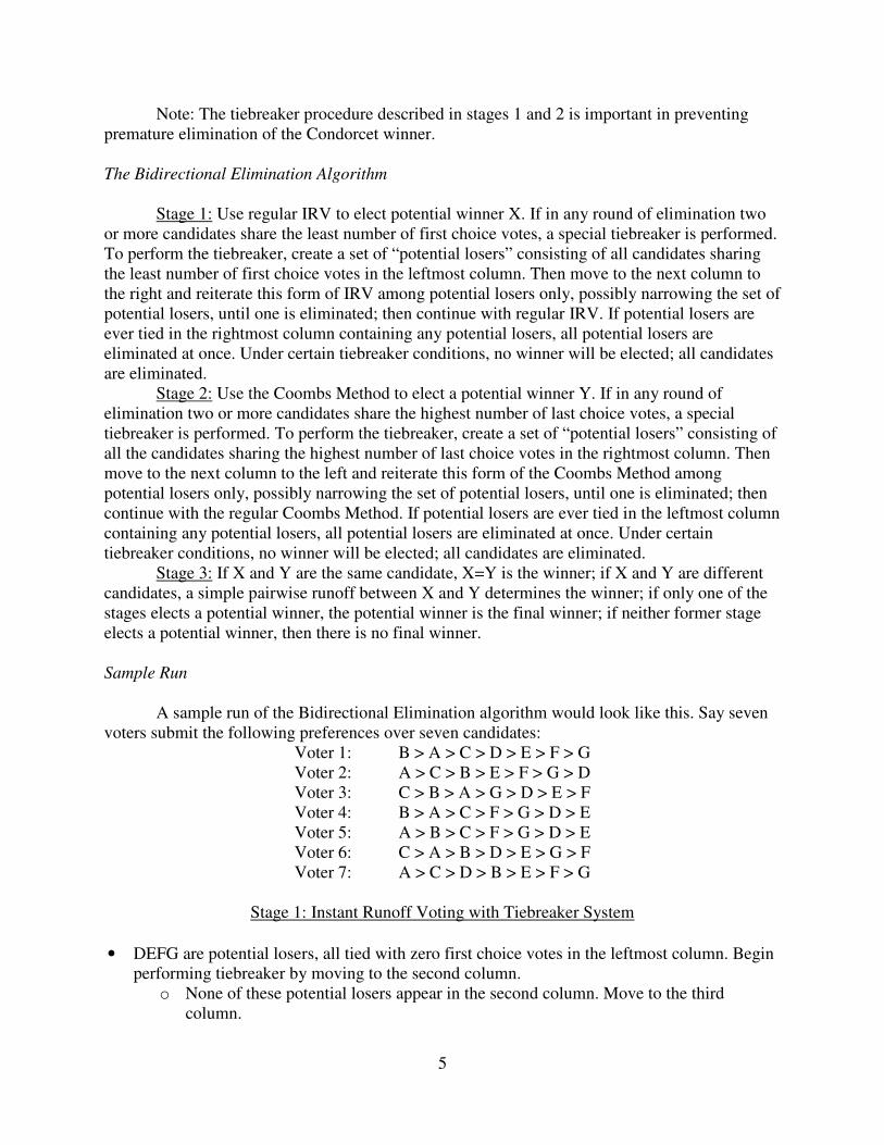
Sample Run

A sample run of the Bidirectional Elimination algorithm would look like this. Say seven

voters submit the following preferences over seven candidates:

Voter 1: B > A > C > D > E > F > G

Voter 2: A > C > B > E > F > G > D

Voter 3: C > B > A > G > D > E > F

Voter 4: B > A > C > F > G > D > E

Voter 5: A > B > C > F > G > D > E

Voter 6: C > A > B > D > E > G > F

Voter 7: A > C > D > B > E > F > G

Stage 1: Instant Runoff Voting with Tiebreaker System

• DEFG are potential losers, all tied with zero first choice votes in the leftmost column. Begin

performing tiebreaker by moving to the second column.

o None of these potential losers appear in the second column. Move to the third

column.

6

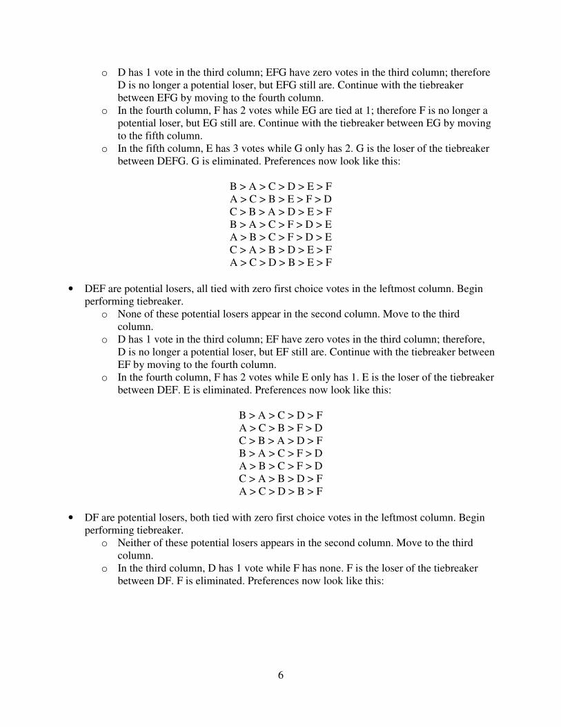
o D has 1 vote in the third column; EFG have zero votes in the third column; therefore

D is no longer a potential loser, but EFG still are. Continue with the tiebreaker

between EFG by moving to the fourth column.

o In the fourth column, F has 2 votes while EG are tied at 1; therefore F is no longer a

potential loser, but EG still are. Continue with the tiebreaker between EG by moving

to the fifth column.

o In the fifth column, E has 3 votes while G only has 2. G is the loser of the tiebreaker

between DEFG. G is eliminated. Preferences now look like this:

B > A > C > D > E > F

A > C > B > E > F > D

C > B > A > D > E > F

B > A > C > F > D > E

A > B > C > F > D > E

C > A > B > D > E > F

A > C > D > B > E > F

• DEF are potential losers, all tied with zero first choice votes in the leftmost column. Begin

performing tiebreaker.

o None of these potential losers appear in the second column. Move to the third

column.

o D has 1 vote in the third column; EF have zero votes in the third column; therefore,

D is no longer a potential loser, but EF still are. Continue with the tiebreaker between

EF by moving to the fourth column.

o In the fourth column, F has 2 votes while E only has 1. E is the loser of the tiebreaker

between DEF. E is eliminated. Preferences now look like this:

B > A > C > D > F

A > C > B > F > D

C > B > A > D > F

B > A > C > F > D

A > B > C > F > D

C > A > B > D > F

A > C > D > B > F

• DF are potential losers, both tied with zero first choice votes in the leftmost column. Begin

performing tiebreaker.

o Neither of these potential losers appears in the second column. Move to the third

column.

o In the third column, D has 1 vote while F has none. F is the loser of the tiebreaker

between DF. F is eliminated. Preferences now look like this:

7

B > A > C > D

A > C > B > D

C > B > A > D

B > A > C > D

A > B > C > D

C > A > B > D

A > C > D > B

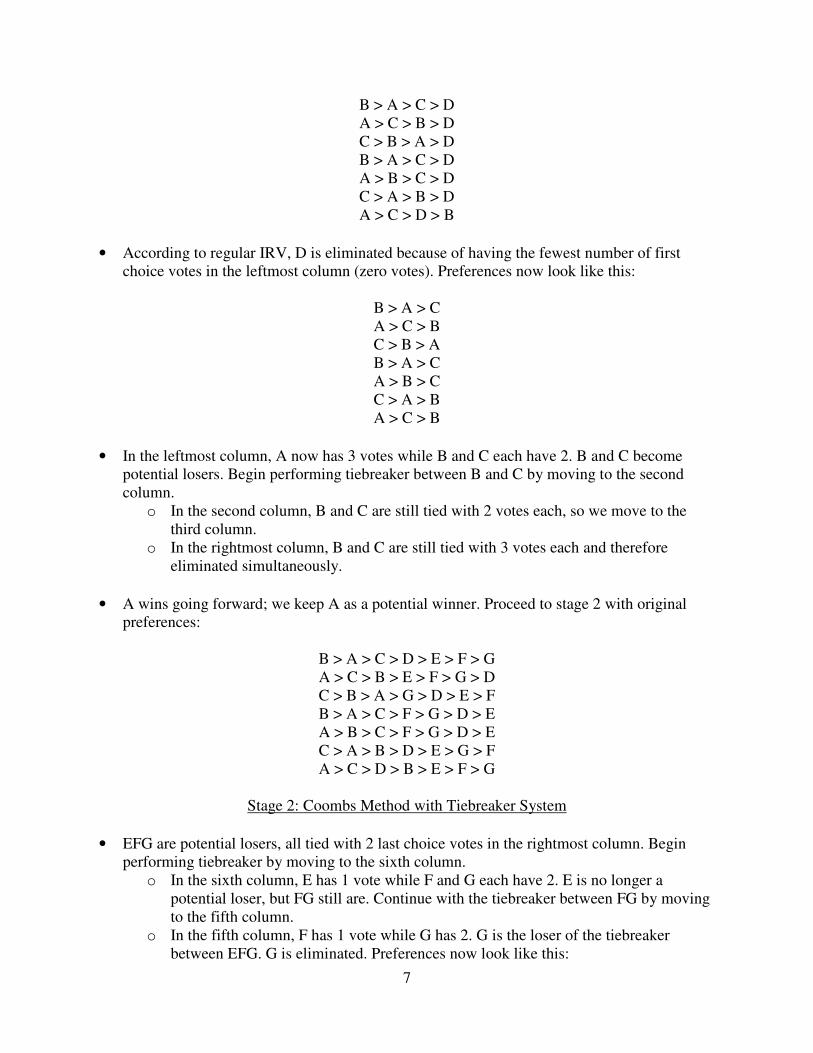
• According to regular IRV, D is eliminated because of having the fewest number of first

choice votes in the leftmost column (zero votes). Preferences now look like this:

B > A > C

A > C > B

C > B > A

B > A > C

A > B > C

C > A > B

A > C > B

• In the leftmost column, A now has 3 votes while B and C each have 2. B and C become

potential losers. Begin performing tiebreaker between B and C by moving to the second

column.

o In the second column, B and C are still tied with 2 votes each, so we move to the

third column.

o In the rightmost column, B and C are still tied with 3 votes each and therefore

eliminated simultaneously.

• A wins going forward; we keep A as a potential winner. Proceed to stage 2 with original

preferences:

B > A > C > D > E > F > G

A > C > B > E > F > G > D

C > B > A > G > D > E > F

B > A > C > F > G > D > E

A > B > C > F > G > D > E

C > A > B > D > E > G > F

A > C > D > B > E > F > G

Stage 2: Coombs Method with Tiebreaker System

• EFG are potential losers, all tied with 2 last choice votes in the rightmost column. Begin

performing tiebreaker by moving to the sixth column.

o In the sixth column, E has 1 vote while F and G each have 2. E is no longer a

potential loser, but FG still are. Continue with the tiebreaker between FG by moving

to the fifth column.

o In the fifth column, F has 1 vote while G has 2. G is the loser of the tiebreaker

between EFG. G is eliminated. Preferences now look like this:

8

B > A > C > D > E > F

A > C > B > E > F > D

C > B > A > D > E > F

B > A > C > F > D > E

A > B > C > F > D > E

C > A > B > D > E > F

A > C > D > B > E > F

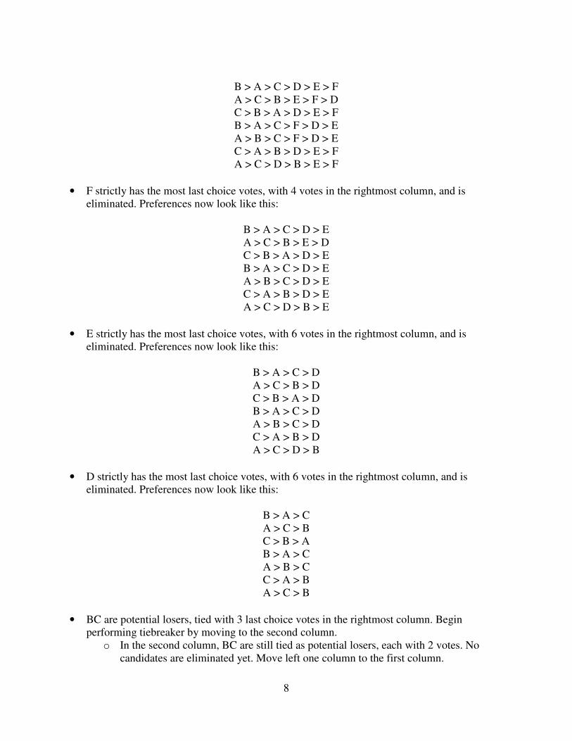
• F strictly has the most last choice votes, with 4 votes in the rightmost column, and is

eliminated. Preferences now look like this:

B > A > C > D > E

A > C > B > E > D

C > B > A > D > E

B > A > C > D > E

A > B > C > D > E

C > A > B > D > E

A > C > D > B > E

• E strictly has the most last choice votes, with 6 votes in the rightmost column, and is


B > A > C > D

A > C > B > D

C > B > A > D

B > A > C > D

A > B > C > D

C > A > B > D

A > C > D > B

• D strictly has the most last choice votes, with 6 votes in the rightmost column, and is


B > A > C

A > C > B

C > B > A

B > A > C

A > B > C

C > A > B

A > C > B

• BC are potential losers, tied with 3 last choice votes in the rightmost column. Begin

performing tiebreaker by moving to the second column.

o In the second column, BC are still tied as potential losers, each with 2 votes. No

candidates are eliminated yet. Move left one column to the first column.

9

o In the first and leftmost column, BC are still tied as potential losers, each with 2

votes, and thus both are eliminated.

• A wins going backward; we keep A as a potential winner. Proceed to stage 3 with potential

winner(s).

Stage 3: Pairwise Runoff

• If different candidates had been elected in stages 1 and 2, a pairwise runoff between the two

potential winners would take place to elect the final winner. In both stages 1 and 2, A is the

potential winner and therefore the actual winner of the election using Bidirectional

Elimination.

Non-Monotonic

Bidirectional Elimination fails the monotonicity criterion and is therefore not strategy-

proof. The preferences below are susceptible to tactical voting.

# Voters True Preferences

4 A > B > C

3 B > C > A

2 C > A > B

IRV and Coombs would each elect A in this case, so Bidirectional Elimination also elects

A. However, a voter with preferences (B>C>A) could simply state falsely that his preferences

were (C>A>B). Preferences would then look like this:

# Voters Reported Preferences

4 A > B > C

2 B > C > A

3 C > A > B

Now, IRV elects C; Coombs elects A; and C wins with Bidirectional Elimination when

compared pairwise with A. By misreporting preferences, a voter was able to improve his

outcome, now getting his second choice instead of his third choice.

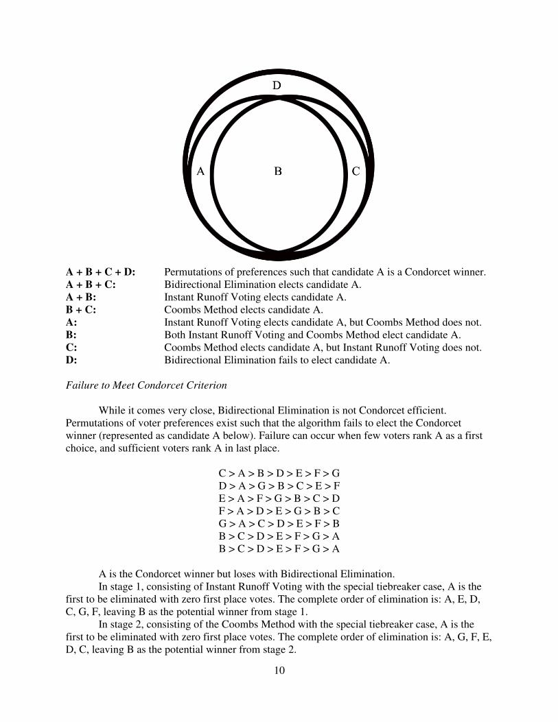
Visualization

The circle below, not to scale, represents an arbitrary space for N>3 candidates and M>4

voters containing permutations of voter preferences.

10

A + B + C + D: Permutations of preferences such that candidate A is a Condorcet winner.

A + B + C: Bidirectional Elimination elects candidate A.

A + B: Instant Runoff Voting elects candidate A.

B + C: Coombs Method elects candidate A.

A: Instant Runoff Voting elects candidate A, but Coombs Method does not.

B: Both Instant Runoff Voting and Coombs Method elect candidate A.

C: Coombs Method elects candidate A, but Instant Runoff Voting does not.

D: Bidirectional Elimination fails to elect candidate A.

Failure to Meet Condorcet Criterion

While it comes very close, Bidirectional Elimination is not Condorcet efficient.

Permutations of voter preferences exist such that the algorithm fails to elect the Condorcet

winner (represented as candidate A below). Failure can occur when few voters rank A as a first

choice, and sufficient voters rank A in last place.

C > A > B > D > E > F > G

D > A > G > B > C > E > F

E > A > F > G > B > C > D

F > A > D > E > G > B > C

G > A > C > D > E > F > B

B > C > D > E > F > G > A

B > C > D > E > F > G > A

A is the Condorcet winner but loses with Bidirectional Elimination.

In stage 1, consisting of Instant Runoff Voting with the special tiebreaker case, A is the

first to be eliminated with zero first place votes. The complete order of elimination is: A, E, D,

C, G, F, leaving B as the potential winner from stage 1.

In stage 2, consisting of the Coombs Method with the special tiebreaker case, A is the

first to be eliminated with zero first place votes. The complete order of elimination is: A, G, F, E,

D, C, leaving B as the potential winner from stage 2.

11

In stage 3, B is promoted from potential winner to actual winner, even though a pairwise

runoff between A and B would favor A with 5 votes to 2 votes.

However, Bidirectional Elimination does satisfy the Condorcet loser criterion since IRV

and Coombs both do, while it would only be necessary for either IRV or Coombs to meet the

condition.

When No Condorcet Winner Exists

While Bidirectional Elimination fails to meet the Condorcet criterion, it comes very

close, as shown in section 6. However, as the number of N candidates or M voters increases, the

number of Condorcet winners generally decreases.

When no Condorcet winner exists, there must be new criteria for evaluating the justness

of a voting algorithm. No Condorcet winner exists when votes are tied, or when a cycle is

present.

When votes are tied—such as in the simplest case, when two voters disagree over which

of two candidates to elect—there is no mathematically just way of choosing between candidates.

Bidirectional Elimination does not choose a winner in tie cases. This is not a bad thing;

depending on the nature of the collective decision, either no winner should be elected, or an

alternative method should be used to arbitrarily select a winner.

Electoral cycles can be similar to ties in that no mathematically just winner exists. The

classic example of Condorcet’s paradox—three voters with profiles (A>B>C), (B>C>A), and

(C>A>B) has no clear winner (this is an example of a circular tie). But what if votes are not as

symmetrical? What if we add a fourth voter with preferences (A>B>C)? Now, A is strictly

preferred over B, which is strictly preferred over C; but A and C are tied in a pairwise runoff.

This is no longer a circular tie. While there may still be no clear winner, electing an arbitrary

candidate seems less than ideal: One could argue that B should be eliminated since it is strictly

dominated by A; and one could debate whether C should be eliminated, since while tied with A,

C is still strictly dominated by B. Establishing criteria for justice is more difficult given an

asymmetric cycle like this one.

A Condorcet completion method is required to elect a winner when ambiguities like these

arise. One such completion method uses the “minimax rule” developed by Simpson and Kramer.

This rule gives a score to each candidate as follows. Candidate A1 is paired against A2-N. For

each pairwise comparison, a score is given to A1 equal to the number of votes his opponent has,

minus the number of his own votes. The maximum of these scores is recorded as W1 (there are

various ways of calculating a W score; this one, called using margins, is the simplest). The

minimum of (W1…N) corresponds to the winner.

Andrew Caplin and Barry Nalebuff proposed a system based on Simpson and Kramer’s

minimax using a “64%-majority rule” that can in fact eliminate all electoral cycles given a

restriction on individual preferences, and on the distribution of preferences.

Bidirectional Elimination may not eliminate electoral cycles, but the mechanism does

satisfy other pleasant, though informal, criteria. The IRV stage of the mechanism will rarely

eliminate a candidate whom voters find appealing, while the Coombs stage will rarely elect a

candidate whom voters find unappealing—and between the two stages, the better candidate is

always chosen.

12

5. Logic Proofs for IRV, Coombs Method, and Bidirectional Elimination

IRV, Coombs Method, and Bidirectional Elimination meet the Condorcet criterion in

certain specific combinations of N candidates and M voters. In this section I examine for which

sets of [N candidates, M voters] each voting system meets the criterion.

For consistency and ease of notation, candidate “A” will be assumed to be the Condorcet

winner.

We will ignore two trivial cases, [1 candidate, M voters] and [N candidates, 1 voter], in

which voters have no choice between candidates, or one voter has the ultimate choice (a situation

similar to dictatorship). Tie and cyclical cases are not discussed here. I am primarily concerned

with electing the Condorcet winner when one exists.

Logic Proofs: Instant Runoff Voting

Instant Runoff Voting, the weakest of the three voting mechanisms studied here, meets

the Condorcet criterion for up to 2 voters and N candidates, or M voters and up to 2 candidates.

N candidates, 2 voters

When only two voters are present, a Condorcet winner can exist only when a tie does not

exist; that is, when the voters agree on the candidate to be chosen. Both candidates have

therefore ranked this candidate (candidate A) as their first choice. All other N-1 candidates will

be eliminated at once, leaving A as the winner from IRV.

2 candidates, M voters

When only two candidates are present, a Condorcet winner exists when either M is odd,

or M is even but the two candidates are not tied in their votes received. In both cases, candidate

A captures more than 50% of the voters. If this is the case, the non-A candidate will be

eliminated in the first and only iteration of IRV.

Logic Proofs: Coombs Method

The Coombs method, which meets the Condorcet criterion in a larger set of

candidate/voter combinations, works consistently for up to 4 voters and N candidates, or M

voters and up to 2 candidates.


When only two voters are present, a Condorcet winner can exist only when a tie does not

exist; that is, when the voters agree on the candidate to be chosen. Both candidates have

therefore ranked this candidate (candidate A) as their first choice, and the losing candidates

(candidate non-A) as their second and last choice. All other N-1 candidates will be eliminated

systematically until only A remains from the Coombs Method.

13


To preserve the existence of a Condorcet winner under these conditions, only one of the

three voters may rank a given non-A candidate above A; otherwise, at least two-thirds of the

voters would prefer a non-A candidate over A.

When columns of preferences are drawn, while N>1 (a winner as not yet been found, as

multiple candidates remain), it follows that A can appear in the rightmost column at most once.

If A were to appear in the rightmost column more than once, at least one non-A would be

preferred in majority over A. This is impossible, as A is the Condorcet winner.

If A does appear in the rightmost column once, either (1) the same non-A is now ranked

in last-place by two voters, in which case this non-A is eliminated, or (2) three different

candidates appear in the last column, in which case A cannot be eliminated in the tiebreaker,

because one of the other two potential losers will be eliminated first. This is because as we move

leftward through columns, A cannot appear before another candidate: At least three voters rank

every other candidate below A.

If A appears in the rightmost column zero times, it will not be eliminated in this round of

the Coombs Method.

Candidate A can never be eliminated as the algorithm iterates.

Under [N candidates, 3 voters] conditions, Candidate A can never be eliminated using the

Coombs method. A will always win.


This proof is directly parallel to the [N candidates, 3 voters] proof.

To preserve the existence of a Condorcet winner under these conditions, only one of the

four voters may rank a given non-A candidate above A; otherwise, a tie could exist, or a majority

of the voters could prefer a non-A candidate over A.

When columns of preferences are drawn, while N>1 (a winner as not yet been found, as

multiple candidates remain), it follows that A can appear in the rightmost column at most once.

If A were to appear in the rightmost column more than once, at least one non-A would be

preferred in majority over A. This is impossible, as A is the Condorcet winner.

If A does appear in the rightmost column once, either (1) a non-A is eliminated right

away, or (2) all different candidates appear in the last column, in which case A cannot be

eliminated in the tiebreaker, because one of the other three potential losers must be eliminated

first. This is because as we move leftward through columns, A cannot appear before another

candidate: At least three voters rank every other candidate below A.

If A appears in the rightmost column zero times, it will not be eliminated in this round of

the Coombs Method.

Candidate A can never be eliminated as the algorithm iterates.

Under [N candidates, 4 voters] conditions, Candidate A can never be eliminated using the

Coombs method. A will always win.

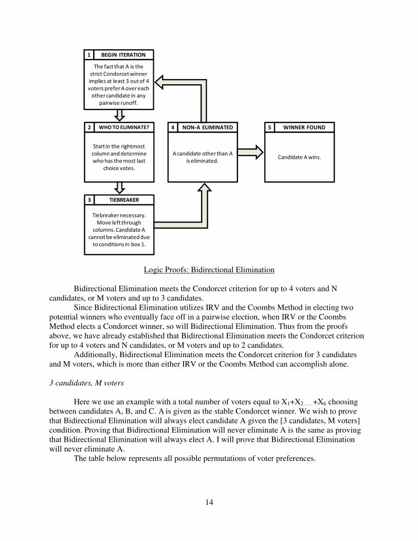
The following diagram illustrates the steps required for understanding the proof.

14

The fact that A is the

strict Condorcet winner

implies at least 3 out of 4

voters prefer A over each

other candidate in any

pairwise runoff.

Start in the rightmost

column and determine

who has the most last

choice votes.

A candidate other than A

is eliminated. Candidate A wins.

Tiebreakernecessary.

Move left through

columns. Candidate A

cannot be eliminated due

to conditions in box 1.

1

2

3

4 5

BEGIN ITERATION

WHO TO ELIMINATE?

TIEBREAKER

NON-A ELIMINATED WINNER FOUND

Logic Proofs: Bidirectional Elimination

Bidirectional Elimination meets the Condorcet criterion for up to 4 voters and N

candidates, or M voters and up to 3 candidates.

Since Bidirectional Elimination utilizes IRV and the Coombs Method in electing two

potential winners who eventually face off in a pairwise election, when IRV or the Coombs

Method elects a Condorcet winner, so will Bidirectional Elimination. Thus from the proofs

above, we have already established that Bidirectional Elimination meets the Condorcet criterion

for up to 4 voters and N candidates, or M voters and up to 2 candidates.

Additionally, Bidirectional Elimination meets the Condorcet criterion for 3 candidates

and M voters, which is more than either IRV or the Coombs Method can accomplish alone.

3 candidates, M voters

Here we use an example with a total number of voters equal to X1+X2 . . . +X6 choosing

between candidates A, B, and C. A is given as the stable Condorcet winner. We wish to prove

that Bidirectional Elimination will always elect candidate A given the [3 candidates, M voters]

condition. Proving that Bidirectional Elimination will never eliminate A is the same as proving

that Bidirectional Elimination will always elect A. I will prove that Bidirectional Elimination

will never eliminate A.

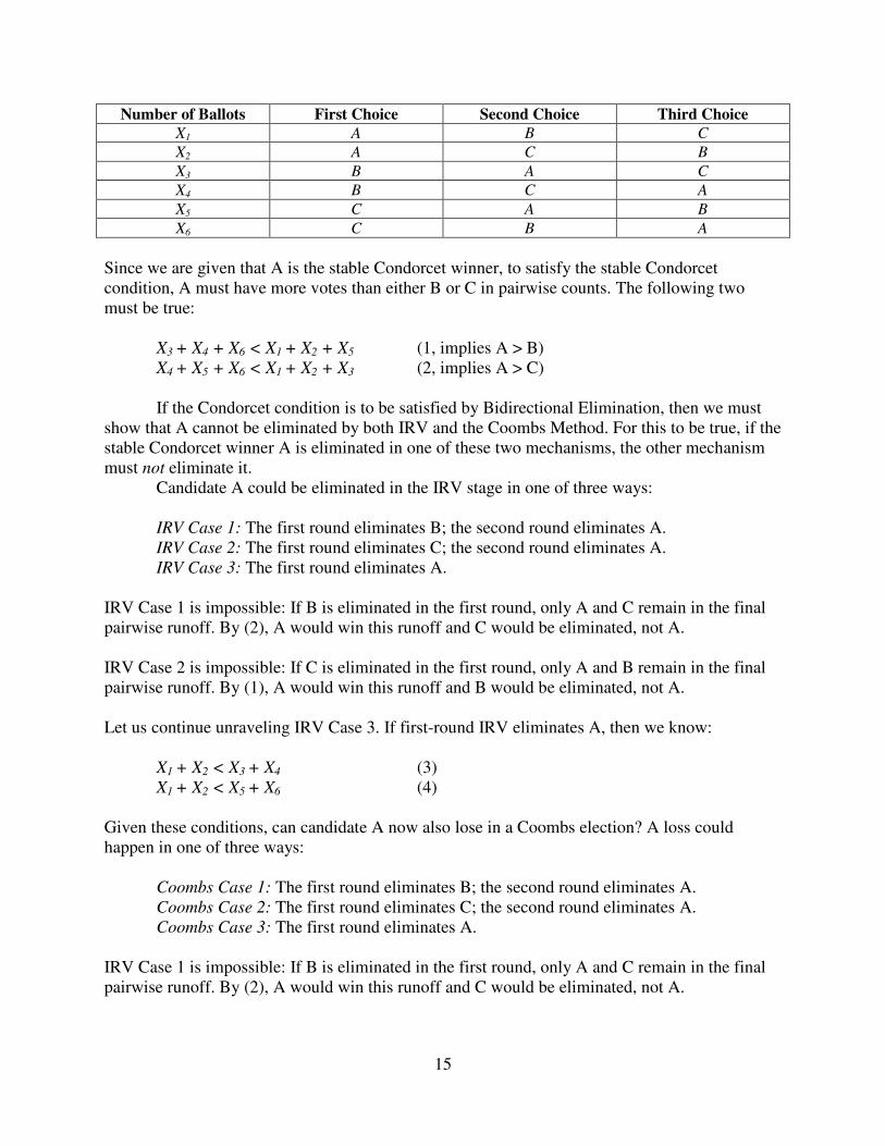
The table below represents all possible permutations of voter preferences.

15

Number of Ballots First Choice Second Choice Third Choice

X1 A B C

X2 A C B

X3 B A C

X4 B C A

X5 C A B

X6 C B A

Since we are given that A is the stable Condorcet winner, to satisfy the stable Condorcet

condition, A must have more votes than either B or C in pairwise counts. The following two

must be true:

X3 + X4 + X6 < X1 + X2 + X5 (1, implies A > B)

X4 + X5 + X6 < X1 + X2 + X3 (2, implies A > C)

If the Condorcet condition is to be satisfied by Bidirectional Elimination, then we must

show that A cannot be eliminated by both IRV and the Coombs Method. For this to be true, if the

stable Condorcet winner A is eliminated in one of these two mechanisms, the other mechanism

must not eliminate it.

Candidate A could be eliminated in the IRV stage in one of three ways:

IRV Case 1: The first round eliminates B; the second round eliminates A.

IRV Case 2: The first round eliminates C; the second round eliminates A.

IRV Case 3: The first round eliminates A.

IRV Case 1 is impossible: If B is eliminated in the first round, only A and C remain in the final

pairwise runoff. By (2), A would win this runoff and C would be eliminated, not A.

IRV Case 2 is impossible: If C is eliminated in the first round, only A and B remain in the final

pairwise runoff. By (1), A would win this runoff and B would be eliminated, not A.

Let us continue unraveling IRV Case 3. If first-round IRV eliminates A, then we know:

X1 + X2 < X3 + X4 (3)

X1 + X2 < X5 + X6 (4)

Given these conditions, can candidate A now also lose in a Coombs election? A loss could

happen in one of three ways:

Coombs Case 1: The first round eliminates B; the second round eliminates A.

Coombs Case 2: The first round eliminates C; the second round eliminates A.

Coombs Case 3: The first round eliminates A.

IRV Case 1 is impossible: If B is eliminated in the first round, only A and C remain in the final

pairwise runoff. By (2), A would win this runoff and C would be eliminated, not A.

16

IRV Case 2 is impossible: If C is eliminated in the first round, only A and B remain in the final

pairwise runoff. By (1), A would win this runoff and B would be eliminated, not A.

This leaves us with only Coombs Case 3—the first round eliminates A—which would require the

following to hold:

X1 + X3 < X4 + X6 (5)

X2 + X5 < X4 + X6 (6)

From (1) and (3), we can show algebraically,

X6 < X5 (7)


X2 < X4 (8)


X3 < X1 (9)


X4 < X3 (10)


X1 < X6 (11)


X5 < X2 (12)

The following chain can be derived from numbers (7) through (12) above:

X5 < X 2 < X4 < X3 < X1 < X6 < X5

Since X5 cannot appear on both sides of the inequality, Coombs Case 3 must also be

impossible. We have just shown that it is impossible for candidate A to be eliminated by IRV,

and also by the Coombs Method. It is therefore impossible for A to be eliminated by

Bidirectional Elimination under these conditions.

Bidirectional Elimination always elects the Condorcet winner given the [3 candidates, M

voters] condition.

This proof can be visualized in a tree.

17

Candidate A, the

Condorcet winner, is

eliminated in the IRV

stage in one of three

ways:

Candidate B is eliminated

in the first round.

Candidate A is eliminated

in the second round.

Candidate C is eliminated

in the first round.




in the first round.

Candidate B is eliminated

in the first round.



Candidate C is eliminated

in the first round.




in the first round.

Impossible Impossible Possible

Impossible Impossible Impossible

Candidate A is also

eliminated in the

Coombs stage one of

three ways:

6. Experimentation via Computer Simulation

A Program to Simulate Voting

Jaehyun Park generously wrote a program according to my specifications to test the

results of IRV, the Coombs Method, and Bidirectional Elimination for various social preference

profiles. The simulation takes in three inputs: N candidates, M voters, and X cases. Here we

define “social preference profile” as the set of ranked preferences for all voters V0…M. When a

user enters X=0, the program will test all possible permutations of social preference profiles

exactly once and output results. (For example, for 2 voters and 3 candidates, V1 has 6 possible

rankings, and V2 has 6 possible rankings, for a total of 36 possible social preference profiles.

Entering X=0 tests each one of these.) When a user enters X>0, the program will create X

random social preference profiles and perform the algorithms on each one. Since these profiles

are random when X>0, it is possible, though rare as M and N increase, for duplicate profiles to

be tested. This duplication is generally expected of Monte Carlo experiments, and in this

experiment does not significantly affect results.

Outputs of the simulation include:

18

• Q, number of total cases, or social preference profiles, tested. Q is equal to X when X>0, or

(N!)M

when X=0. Individual preferences were restricted to include only sets in which each

voter gave a ranking to every candidate. That is, if options A through E were available, each

voter included options A through E in his individual preference profile, omitting no option

from his ordering. Removing this domain restriction would expand the total number of

possible social preference profiles to (N! + N!/2! + N!/3! . . . + 1)M

, making the program

unfeasible.

• R, number of cases where A is the Condorcet winner. The program labels one of the

candidates as candidate A, and tests permutations of preferences to determine whether A is a

stable Condorcet winner.

• R/Q, percentage of cases where A is a Condorcet winner. This calculation performs R/Q, the

number of times that A is a Condorcet winner divided by the number of total cases tested.

• N*R, number of cases a Condorcet winner exists. By symmetry, we can multiply R by the

number of candidates to determine for how many permutations a Condorcet winner exists.

• (N*R)/Q, percentage of cases where there is a Condorcet winner. Dividing N*R by the total

number of cases tells us the percentage of cases for which a Condorcet winner exists.

• S, the IRV success figure. This is equal to the number of times that A is the Condorcet

winner, and Instant Runoff Voting elects A.

• S/R, the IRV success ratio. Dividing S by the number of cases where A is the Condorcet

winner returns a valuable percentage.

• T, the Coombs Method success figure. This is equal to the number of times that A is the

Condorcet winner, and the Coombs Method elects A.

• T/R, the Coombs Method success ratio. Dividing R by the number of cases where A is the

Condorcet winner returns a valuable percentage.

• U, the Bidirectional Elimination success figure. This is equal to the number of times that A

is the Condorcet winner, and Bidirectional Elimination elects A.

• U/R, the Bidirectional Elimination success ratio. Dividing U by the number of cases where

A is the Condorcet winner returns a valuable percentage.

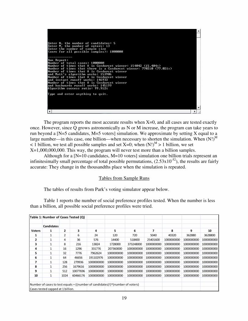
A sample run of the simulation looks like this:

19

The program reports the most accurate results when X=0, and all cases are tested exactly

once. However, since Q grows astronomically as N or M increase, the program can take years to

run beyond a [N=5 candidates, M=5 voters] simulation. We approximate by setting X equal to a

large number—in this case, one billion—when necessary to shorten the simulation. When (N!)M

< 1 billion, we test all possible samples and set X=0; when (N!)M

> 1 billion, we set

X=1,000,000,000. This way, the program will never test more than a billion samples.

Although for a [N=10 candidates, M=10 voters] simulation one billion trials represent an

infinitesimally small percentage of total possible permutations, (2.53x10-52

), the results are fairly

accurate: They change in the thousandths place when the simulation is repeated.

Tables from Sample Runs

The tables of results from Park’s voting simulator appear below.

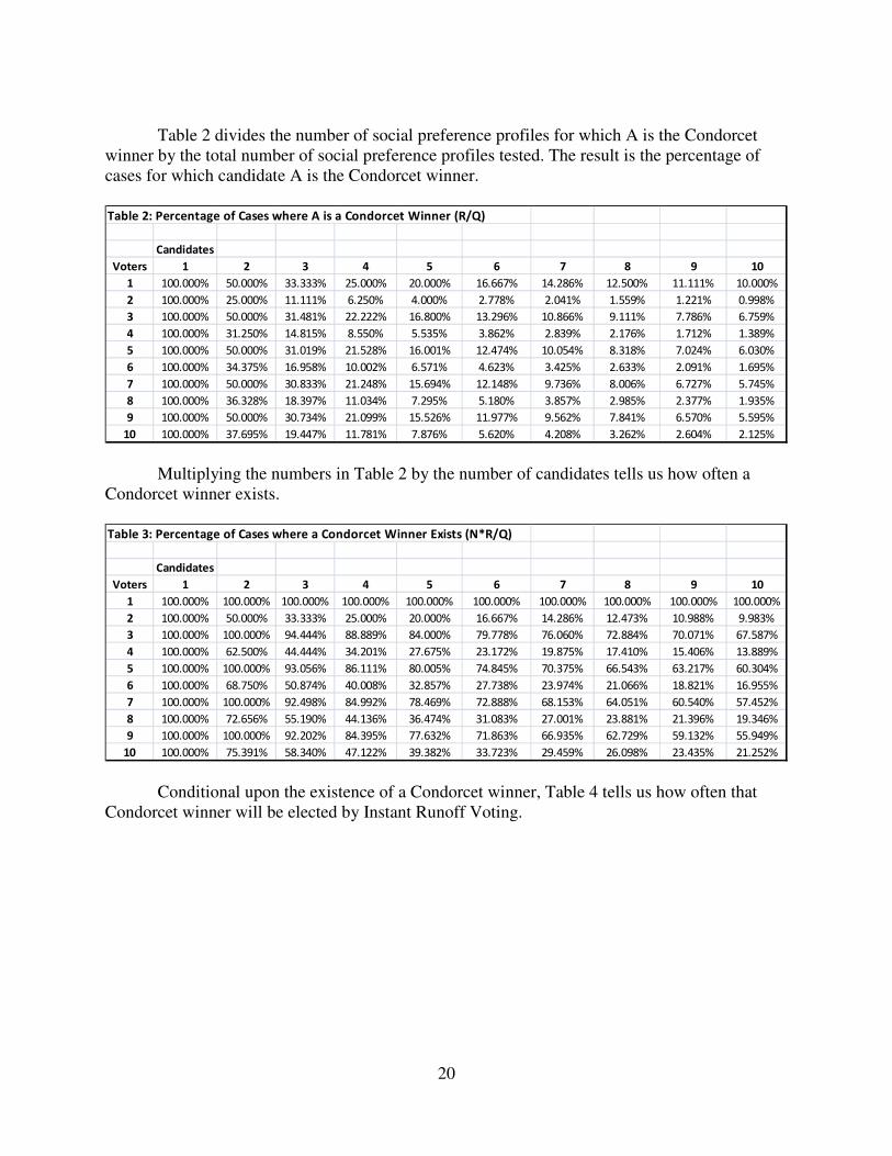
Table 1 reports the number of social preference profiles tested. When the number is less

than a billion, all possible social preference profiles were tried.

Table 1: Number of Cases Tested (Q)

Candidates

Voters 1 2 3 4 5 6 7 8 9 10

1 1 2 6 24 120 720 5040 40320 362880 3628800

2 1 4 36 576 14400 518400 25401600 1000000000 1000000000 1000000000

3 1 8 216 13824 1728000 373248000 1000000000 1000000000 1000000000 1000000000

4 1 16 1296 331776 207360000 1000000000 1000000000 1000000000 1000000000 1000000000

5 1 32 7776 7962624 1000000000 1000000000 1000000000 1000000000 1000000000 1000000000

6 1 64 46656 191102976 1000000000 1000000000 1000000000 1000000000 1000000000 1000000000

7 1 128 279936 1000000000 1000000000 1000000000 1000000000 1000000000 1000000000 1000000000

8 1 256 1679616 1000000000 1000000000 1000000000 1000000000 1000000000 1000000000 1000000000

9 1 512 10077696 1000000000 1000000000 1000000000 1000000000 1000000000 1000000000 1000000000

10 1 1024 60466176 1000000000 1000000000 1000000000 1000000000 1000000000 1000000000 1000000000

Number of cases to test equals = ((number of candidates)!)^(number of voters)

Cases tested capped at 1 billion.

20

Table 2 divides the number of social preference profiles for which A is the Condorcet

winner by the total number of social preference profiles tested. The result is the percentage of

cases for which candidate A is the Condorcet winner.

Table 2: Percentage of Cases where A is a Condorcet Winner (R/Q)

Candidates

Voters 1 2 3 4 5 6 7 8 9 10

1 100.000% 50.000% 33.333% 25.000% 20.000% 16.667% 14.286% 12.500% 11.111% 10.000%

2 100.000% 25.000% 11.111% 6.250% 4.000% 2.778% 2.041% 1.559% 1.221% 0.998%

3 100.000% 50.000% 31.481% 22.222% 16.800% 13.296% 10.866% 9.111% 7.786% 6.759%

4 100.000% 31.250% 14.815% 8.550% 5.535% 3.862% 2.839% 2.176% 1.712% 1.389%

5 100.000% 50.000% 31.019% 21.528% 16.001% 12.474% 10.054% 8.318% 7.024% 6.030%

6 100.000% 34.375% 16.958% 10.002% 6.571% 4.623% 3.425% 2.633% 2.091% 1.695%

7 100.000% 50.000% 30.833% 21.248% 15.694% 12.148% 9.736% 8.006% 6.727% 5.745%

8 100.000% 36.328% 18.397% 11.034% 7.295% 5.180% 3.857% 2.985% 2.377% 1.935%

9 100.000% 50.000% 30.734% 21.099% 15.526% 11.977% 9.562% 7.841% 6.570% 5.595%

10 100.000% 37.695% 19.447% 11.781% 7.876% 5.620% 4.208% 3.262% 2.604% 2.125%

Multiplying the numbers in Table 2 by the number of candidates tells us how often a

Condorcet winner exists.

Table 3: Percentage of Cases where a Condorcet Winner Exists (N*R/Q)

Candidates

Voters 1 2 3 4 5 6 7 8 9 10

1 100.000% 100.000% 100.000% 100.000% 100.000% 100.000% 100.000% 100.000% 100.000% 100.000%

2 100.000% 50.000% 33.333% 25.000% 20.000% 16.667% 14.286% 12.473% 10.988% 9.983%

3 100.000% 100.000% 94.444% 88.889% 84.000% 79.778% 76.060% 72.884% 70.071% 67.587%

4 100.000% 62.500% 44.444% 34.201% 27.675% 23.172% 19.875% 17.410% 15.406% 13.889%

5 100.000% 100.000% 93.056% 86.111% 80.005% 74.845% 70.375% 66.543% 63.217% 60.304%

6 100.000% 68.750% 50.874% 40.008% 32.857% 27.738% 23.974% 21.066% 18.821% 16.955%

7 100.000% 100.000% 92.498% 84.992% 78.469% 72.888% 68.153% 64.051% 60.540% 57.452%

8 100.000% 72.656% 55.190% 44.136% 36.474% 31.083% 27.001% 23.881% 21.396% 19.346%

9 100.000% 100.000% 92.202% 84.395% 77.632% 71.863% 66.935% 62.729% 59.132% 55.949%

10 100.000% 75.391% 58.340% 47.122% 39.382% 33.723% 29.459% 26.098% 23.435% 21.252%

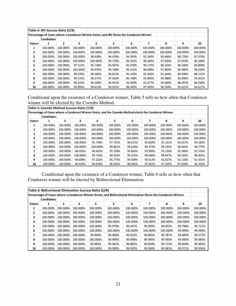
Conditional upon the existence of a Condorcet winner, Table 4 tells us how often that

Condorcet winner will be elected by Instant Runoff Voting.

21

Table 4: IRV Success Ratio (S/R)

Percentage of Cases where a Condorcet Winner Exists, and IRV Elects the Condorcet Winner

Candidates

Voters 1 2 3 4 5 6 7 8 9 10

1 100.000% 100.000% 100.000% 100.000% 100.000% 100.000% 100.000% 100.000% 100.000% 100.000%

2 100.000% 100.000% 100.000% 100.000% 100.000% 100.000% 100.000% 100.000% 100.000% 100.000%

3 100.000% 100.000% 100.000% 98.438% 96.429% 94.359% 92.349% 90.466% 88.720% 87.070%

4 100.000% 100.000% 100.000% 100.000% 99.729% 99.241% 98.560% 97.839% 97.019% 96.168%

5 100.000% 100.000% 97.512% 95.758% 93.947% 92.078% 90.172% 88.326% 86.560% 84.800%

6 100.000% 100.000% 100.000% 99.970% 99.768% 99.313% 98.668% 97.883% 96.989% 96.030%

7 100.000% 100.000% 99.676% 98.360% 96.815% 95.143% 93.403% 91.644% 89.938% 88.212%

8 100.000% 100.000% 99.275% 98.377% 97.563% 96.748% 95.890% 94.986% 94.099% 93.001%

9 100.000% 100.000% 98.332% 96.598% 94.941% 93.309% 91.677% 90.066% 88.497% 86.938%

10 100.000% 100.000% 99.893% 99.613% 99.031% 98.309% 97.493% 96.594% 95.621% 94.627%

Conditional upon the existence of a Condorcet winner, Table 5 tells us how often that Condorcet

winner will be elected by the Coombs Method. Table 5: Coombs Method Success Ratio (T/R)

Percentage of Cases where a Condorcet Winner Exists, and the Coombs Method elects the Condorcet Winner

Candidates

Voters 1 2 3 4 5 6 7 8 9 10

1 100.000% 100.000% 100.000% 100.000% 100.000% 100.000% 100.000% 100.000% 100.000% 100.000%

2 100.000% 100.000% 100.000% 100.000% 100.000% 100.000% 100.000% 100.000% 100.000% 100.000%

3 100.000% 100.000% 100.000% 100.000% 100.000% 100.000% 100.000% 100.000% 100.000% 100.000%

4 100.000% 100.000% 100.000% 100.000% 100.000% 100.000% 100.000% 100.000% 100.000% 100.000%

5 100.000% 100.000% 100.000% 95.758% 97.755% 96.672% 95.820% 95.161% 94.637% 94.183%

6 100.000% 100.000% 100.000% 100.000% 99.862% 99.630% 99.374% 99.143% 98.944% 98.779%

7 100.000% 100.000% 98.054% 96.663% 95.709% 94.863% 93.999% 93.130% 92.286% 91.516%

8 100.000% 100.000% 100.000% 99.716% 99.450% 99.255% 99.060% 98.847% 98.593% 98.305%

9 100.000% 100.000% 98.698% 97.232% 95.775% 94.569% 93.613% 92.827% 92.118% 91.431%

10 100.000% 100.000% 99.429% 99.034% 98.565% 98.082% 97.661% 97.320% 97.039% 96.765%

Conditional upon the existence of a Condorcet winner, Table 6 tells us how often that

Condorcet winner will be elected by Bidirectional Elimination.

Table 6: Bidirectional Elimination Success Ratio (U/R)

Percentage of Cases where a Condorcet Winner Exists, and Bidirectional Elimination Elects the Condorcet Winner

Candidates

Voters 1 2 3 4 5 6 7 8 9 10

1 100.000% 100.000% 100.000% 100.000% 100.000% 100.000% 100.000% 100.000% 100.000% 100.000%

2 100.000% 100.000% 100.000% 100.000% 100.000% 100.000% 100.000% 100.000% 100.000% 100.000%

3 100.000% 100.000% 100.000% 100.000% 100.000% 100.000% 100.000% 100.000% 100.000% 100.000%

4 100.000% 100.000% 100.000% 100.000% 100.000% 100.000% 100.000% 100.000% 100.000% 100.000%

5 100.000% 100.000% 100.000% 100.000% 99.979% 99.947% 99.905% 99.855% 99.798% 99.731%

6 100.000% 100.000% 100.000% 100.000% 100.000% 100.000% 100.000% 100.000% 99.999% 99.998%

7 100.000% 100.000% 100.000% 99.994% 99.968% 99.925% 99.865% 99.787% 99.689% 99.577%

8 100.000% 100.000% 100.000% 100.000% 99.999% 99.998% 99.995% 99.993% 99.990% 99.983%

9 100.000% 100.000% 100.000% 99.983% 99.942% 99.881% 99.804% 99.713% 99.609% 99.485%

10 100.000% 100.000% 100.000% 100.000% 99.999% 99.995% 99.990% 99.981% 99.971% 99.956%

22

Analysis of Results

Existence of a Condorcet Winner

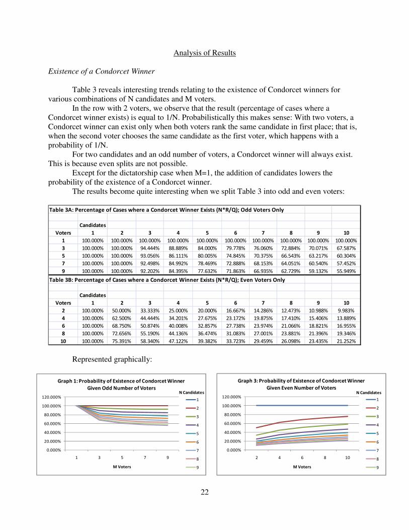
Table 3 reveals interesting trends relating to the existence of Condorcet winners for

various combinations of N candidates and M voters.

In the row with 2 voters, we observe that the result (percentage of cases where a

Condorcet winner exists) is equal to 1/N. Probabilistically this makes sense: With two voters, a

Condorcet winner can exist only when both voters rank the same candidate in first place; that is,

when the second voter chooses the same candidate as the first voter, which happens with a

probability of 1/N.

For two candidates and an odd number of voters, a Condorcet winner will always exist.

This is because even splits are not possible.

Except for the dictatorship case when M=1, the addition of candidates lowers the

probability of the existence of a Condorcet winner.

The results become quite interesting when we split Table 3 into odd and even voters:

Table 3A: Percentage of Cases where a Condorcet Winner Exists (N*R/Q); Odd Voters Only

Candidates

Voters 1 2 3 4 5 6 7 8 9 10

1 100.000% 100.000% 100.000% 100.000% 100.000% 100.000% 100.000% 100.000% 100.000% 100.000%

3 100.000% 100.000% 94.444% 88.889% 84.000% 79.778% 76.060% 72.884% 70.071% 67.587%

5 100.000% 100.000% 93.056% 86.111% 80.005% 74.845% 70.375% 66.543% 63.217% 60.304%

7 100.000% 100.000% 92.498% 84.992% 78.469% 72.888% 68.153% 64.051% 60.540% 57.452%

9 100.000% 100.000% 92.202% 84.395% 77.632% 71.863% 66.935% 62.729% 59.132% 55.949% Table 3B: Percentage of Cases where a Condorcet Winner Exists (N*R/Q); Even Voters Only

Candidates

Voters 1 2 3 4 5 6 7 8 9 10

2 100.000% 50.000% 33.333% 25.000% 20.000% 16.667% 14.286% 12.473% 10.988% 9.983%

4 100.000% 62.500% 44.444% 34.201% 27.675% 23.172% 19.875% 17.410% 15.406% 13.889%

6 100.000% 68.750% 50.874% 40.008% 32.857% 27.738% 23.974% 21.066% 18.821% 16.955%

8 100.000% 72.656% 55.190% 44.136% 36.474% 31.083% 27.001% 23.881% 21.396% 19.346%

10 100.000% 75.391% 58.340% 47.122% 39.382% 33.723% 29.459% 26.098% 23.435% 21.252%

Represented graphically:

0.000%

20.000%

40.000%

60.000%

80.000%

100.000%

120.000%

2 4 6 8 10

M Voters

Graph 3: Probability of Existence of Condorcet Winner

Given Even Number of Voters

1

2

3

4

5

6

7

8

9

N Candidates

0.000%

20.000%

40.000%

60.000%

80.000%

100.000%

120.000%

1 3 5 7 9

M Voters


Given Odd Number of Voters

1

2

3

4

5

6

7

8

9

N Candidates

23

0.000%

20.000%

40.000%

60.000%

80.000%

100.000%

120.000%

1 2 3 4 5 6 7 8 9 10

N Candidates


Given N Candidates and Even M Voters

2

4

6

8

10

M Voters

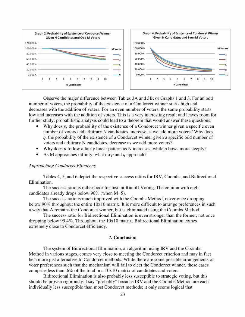
Observe the major difference between Tables 3A and 3B, or Graphs 1 and 3. For an odd

number of voters, the probability of the existence of a Condorcet winner starts high and

decreases with the addition of voters. For an even number of voters, the same probability starts

low and increases with the addition of voters. This is a very interesting result and leaves room for

further study; probabilistic analysis could lead to a theorem that would answer these questions:

• Why does p, the probability of the existence of a Condorcet winner given a specific even

number of voters and arbitrary N candidates, increase as we add more voters? Why does

q, the probability of the existence of a Condorcet winner given a specific odd number of

voters and arbitrary N candidates, decrease as we add more voters?

• Why does p follow a fairly linear pattern as N increases, while q bows more steeply?

• As M approaches infinity, what do p and q approach?

Approaching Condorcet Efficiency

Tables 4, 5, and 6 depict the respective success ratios for IRV, Coombs, and Bidirectional

Elimination.

The success ratio is rather poor for Instant Runoff Voting. The column with eight

candidates already drops below 90% (when M=5).

The success ratio is much improved with the Coombs Method, never once dropping

below 90% throughout the entire 10x10 matrix. It is more difficult to arrange preferences in such

a way that A remains the Condorcet winner, but is eliminated using the Coombs Method.

The success ratio for Bidirectional Elimination is even stronger than the former, not once

dropping below 99.4%. Throughout the 10x10 matrix, Bidirectional Elimination comes

extremely close to Condorcet efficiency.

7. Conclusion

The system of Bidirectional Elimination, an algorithm using IRV and the Coombs

Method in various stages, comes very close to meeting the Condorcet criterion and may in fact

be a more just alternative to Condorcet methods. While there are some possible arrangements of

voter preferences such that the mechanism will fail to elect the Condorcet winner, these cases

comprise less than .6% of the total in a 10x10 matrix of candidates and voters.

Bidirectional Elimination is also probably less susceptible to strategic voting, but this

should be proven rigorously. I say “probably” because IRV and the Coombs Method are each

individually less susceptible than most Condorcet methods; it only seems logical that

0.000%

20.000%

40.000%

60.000%

80.000%

100.000%

120.000%

1 2 3 4 5 6 7 8 9 10

N Candidates


Given N Candidates and Odd M Voters

1

3

5

7

9

M Voters

24

Bidirectional Elimination would be as well. This question leaves room for future study and

experimentation: Given most Condorcet methods’ vulnerability to tactical voting, Bidirectional

Elimination may ironically be more successful at electing the Condorcet winner. I encourage

future economists to rigorously examine the susceptibility of Bidirectional Elimination to

strategic voting, and compare with that of Condorcet methods, as well as IRV and the Coombs

Method individually.

Experimentation for Strategy-Proofness

This study could be facilitated with a program similar to Jaehyun Park’s, that would work

as follows. Given inputs for N candidates and M voters, the program would generate (N!)M

permutations of true preferences for voters V1 through VM. A “case counter” would start at zero.

For each possible permutation of true preferences, the following would happen (a nested for

loop):

(1) The voting algorithm in question would be performed on true preferences, and a

winner W would be elected.

(2) Holding all other voters’ preferences constant, the program would then generate all

remaining (N!-1) false permutations of voter V1’s preferences, and perform the algorithm on

each of these. If at least one set of false preferences existed for V1 such that reporting these false

preferences would elected a candidate whom V1 preferred over W, one would be added to a

“case counter,” and the program would move onto the next set of true preferences, skipping steps

3 and 4.

(3) If nothing had been added to the case counter after trying all permutations of false

preferences for V1, the program would repeat step 2 for V2…M. If at least one set of false

preferences existed for any Vi such that reporting these false preferences would elect a candidate

whom Vi preferred over W, one would be added to a “case counter,” and the program would

move onto the next permutation of true preferences.

(4) If after step 3 no set of false preferences were found for any voter Vi that could

improve his outcome, the “case counter” would remain at its current value, and the next

permutation of true preferences would be tested similarly, until all permutation of true

preferences had been tested.

(5) Dividing the final “case counter” value by (N!)M

would output the percentage of

cases, given N and M as inputs, for which the voting algorithm in question is susceptible to

tactical voting.

The program would need to be designed, as Park designed his, to be capable of random

sampling in addition to testing all cases. As N and M grow, (N!)M

grows astronomically—and

given the number of operations required to conduct this simulation, testing all cases could

require vast amounts of time. A Monte Carlo method will be necessary.

Implementation

I recommend that Bidirectional Elimination be implemented in small to medium scale

elections first. Adopting Bidirectional Elimination at larger scale elections, such as state and

national elections, may be politically unfeasible; the mechanism would likely be met with

resistance and confusion initially. The mechanism is difficult to understand and may be rejected

by voting populations. Small scale elections could include committee meetings or corporate

elections. Medium scale elections would include elections with larger voting populations in the

25

order of thousands, such as student elections at universities, or voting at the Oscars. Having

demonstrated a willingness to improve its voting mechanism, the Academy of Motion Picture

Arts and Sciences might feel motivated to replace IRV with Bidirectional Elimination. Adoption

into large elections is a worthy long-term goal.

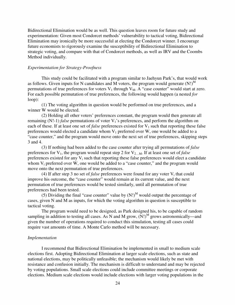
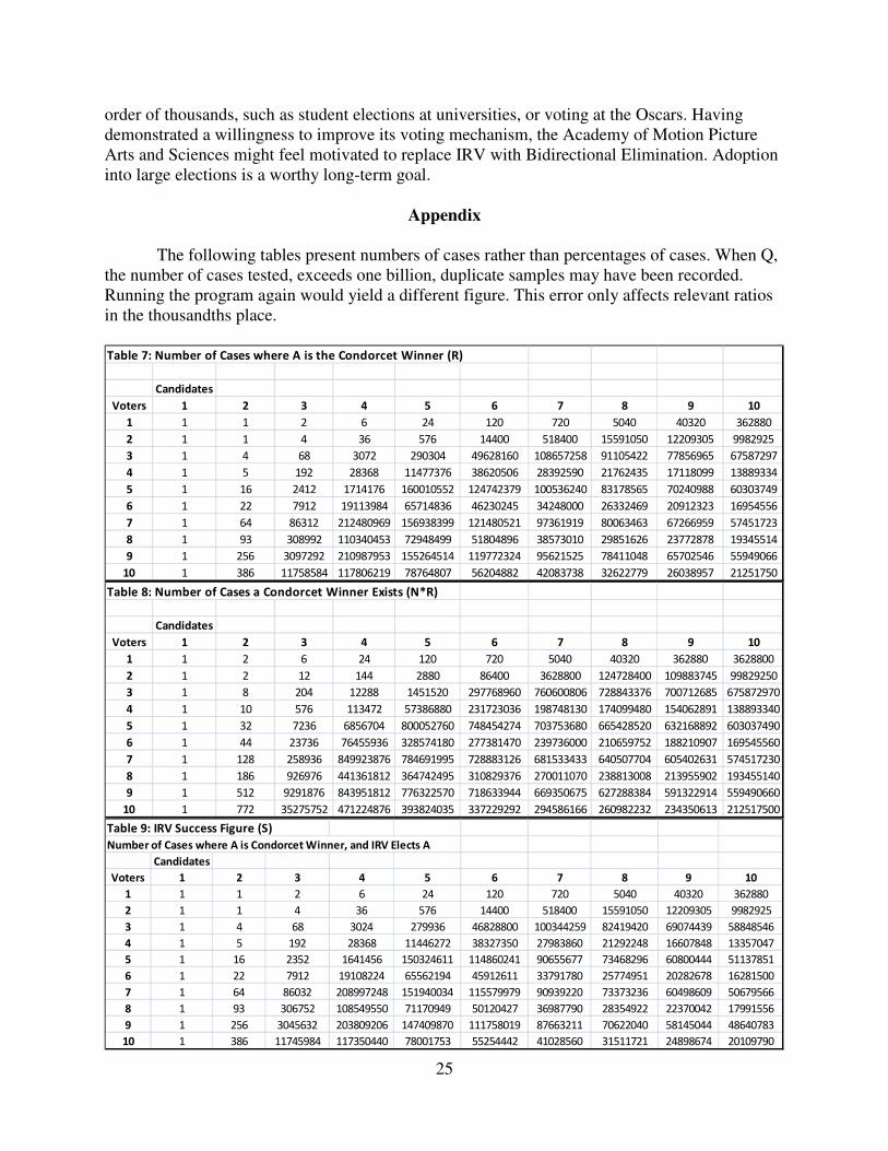
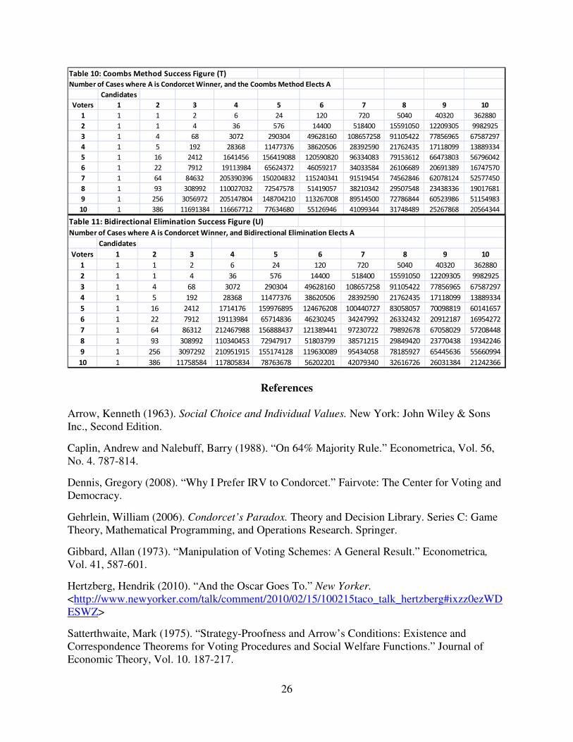
Appendix

The following tables present numbers of cases rather than percentages of cases. When Q,

the number of cases tested, exceeds one billion, duplicate samples may have been recorded.

Running the program again would yield a different figure. This error only affects relevant ratios

in the thousandths place.

Table 7: Number of Cases where A is the Condorcet Winner (R)

Candidates

Voters 1 2 3 4 5 6 7 8 9 10

1 1 1 2 6 24 120 720 5040 40320 362880

2 1 1 4 36 576 14400 518400 15591050 12209305 9982925

3 1 4 68 3072 290304 49628160 108657258 91105422 77856965 67587297

4 1 5 192 28368 11477376 38620506 28392590 21762435 17118099 13889334

5 1 16 2412 1714176 160010552 124742379 100536240 83178565 70240988 60303749

6 1 22 7912 19113984 65714836 46230245 34248000 26332469 20912323 16954556

7 1 64 86312 212480969 156938399 121480521 97361919 80063463 67266959 57451723

8 1 93 308992 110340453 72948499 51804896 38573010 29851626 23772878 19345514

9 1 256 3097292 210987953 155264514 119772324 95621525 78411048 65702546 55949066

10 1 386 11758584 117806219 78764807 56204882 42083738 32622779 26038957 21251750 Table 8: Number of Cases a Condorcet Winner Exists (N*R)

Candidates

Voters 1 2 3 4 5 6 7 8 9 10

1 1 2 6 24 120 720 5040 40320 362880 3628800

2 1 2 12 144 2880 86400 3628800 124728400 109883745 99829250

3 1 8 204 12288 1451520 297768960 760600806 728843376 700712685 675872970

4 1 10 576 113472 57386880 231723036 198748130 174099480 154062891 138893340

5 1 32 7236 6856704 800052760 748454274 703753680 665428520 632168892 603037490

6 1 44 23736 76455936 328574180 277381470 239736000 210659752 188210907 169545560

7 1 128 258936 849923876 784691995 728883126 681533433 640507704 605402631 574517230

8 1 186 926976 441361812 364742495 310829376 270011070 238813008 213955902 193455140

9 1 512 9291876 843951812 776322570 718633944 669350675 627288384 591322914 559490660

10 1 772 35275752 471224876 393824035 337229292 294586166 260982232 234350613 212517500 Table 9: IRV Success Figure (S)

Number of Cases where A is Condorcet Winner, and IRV Elects A

Candidates

Voters 1 2 3 4 5 6 7 8 9 10

1 1 1 2 6 24 120 720 5040 40320 362880

2 1 1 4 36 576 14400 518400 15591050 12209305 9982925

3 1 4 68 3024 279936 46828800 100344259 82419420 69074439 58848546

4 1 5 192 28368 11446272 38327350 27983860 21292248 16607848 13357047

5 1 16 2352 1641456 150324611 114860241 90655677 73468296 60800444 51137851

6 1 22 7912 19108224 65562194 45912611 33791780 25774951 20282678 16281500

7 1 64 86032 208997248 151940034 115579979 90939220 73373236 60498609 50679566

8 1 93 306752 108549550 71170949 50120427 36987790 28354922 22370042 17991556

9 1 256 3045632 203809206 147409870 111758019 87663211 70622040 58145044 48640783

10 1 386 11745984 117350440 78001753 55254442 41028560 31511721 24898674 20109790

26

Table 10: Coombs Method Success Figure (T)

Number of Cases where A is Condorcet Winner, and the Coombs Method Elects A

Candidates

Voters 1 2 3 4 5 6 7 8 9 10

1 1 1 2 6 24 120 720 5040 40320 362880

2 1 1 4 36 576 14400 518400 15591050 12209305 9982925

3 1 4 68 3072 290304 49628160 108657258 91105422 77856965 67587297

4 1 5 192 28368 11477376 38620506 28392590 21762435 17118099 13889334

5 1 16 2412 1641456 156419088 120590820 96334083 79153612 66473803 56796042

6 1 22 7912 19113984 65624372 46059217 34033584 26106689 20691389 16747570

7 1 64 84632 205390396 150204832 115240341 91519454 74562846 62078124 52577450

8 1 93 308992 110027032 72547578 51419057 38210342 29507548 23438336 19017681

9 1 256 3056972 205147804 148704210 113267008 89514500 72786844 60523986 51154983

10 1 386 11691384 116667712 77634680 55126946 41099344 31748489 25267868 20564344 Table 11: Bidirectional Elimination Success Figure (U)

Number of Cases where A is Condorcet Winner, and Bidirectional Elimination Elects A

Candidates

Voters 1 2 3 4 5 6 7 8 9 10

1 1 1 2 6 24 120 720 5040 40320 362880

2 1 1 4 36 576 14400 518400 15591050 12209305 9982925

3 1 4 68 3072 290304 49628160 108657258 91105422 77856965 67587297

4 1 5 192 28368 11477376 38620506 28392590 21762435 17118099 13889334

5 1 16 2412 1714176 159976895 124676208 100440727 83058057 70098819 60141657

6 1 22 7912 19113984 65714836 46230245 34247992 26332432 20912187 16954272

7 1 64 86312 212467988 156888437 121389441 97230722 79892678 67058029 57208448

8 1 93 308992 110340453 72947917 51803799 38571215 29849420 23770438 19342246

9 1 256 3097292 210951915 155174128 119630089 95434058 78185927 65445636 55660994

10 1 386 11758584 117805834 78763678 56202201 42079340 32616726 26031384 21242366

References

Arrow, Kenneth (1963). Social Choice and Individual Values. New York: John Wiley & Sons

Inc., Second Edition.

Caplin, Andrew and Nalebuff, Barry (1988). “On 64% Majority Rule.” Econometrica, Vol. 56,

No. 4. 787-814.

Dennis, Gregory (2008). “Why I Prefer IRV to Condorcet.” Fairvote: The Center for Voting and

Democracy.

Gehrlein, William (2006). Condorcet’s Paradox. Theory and Decision Library. Series C: Game

Theory, Mathematical Programming, and Operations Research. Springer.

Gibbard, Allan (1973). “Manipulation of Voting Schemes: A General Result.” Econometrica,

Vol. 41, 587-601.

Hertzberg, Hendrik (2010). “And the Oscar Goes To.” New Yorker.

<http://www.newyorker.com/talk/comment/2010/02/15/100215taco_talk_hertzberg#ixzz0ezWD

ESWZ>

Satterthwaite, Mark (1975). “Strategy-Proofness and Arrow’s Conditions: Existence and

Correspondence Theorems for Voting Procedures and Social Welfare Functions.” Journal of

Economic Theory, Vol. 10. 187-217.

voting with bidirectional elimination - economics · voting with bidirectional elimination matthew...

Documents