vortex blob methods applied to interfacial motionbeale/papers/baker.pdf · vortex blob methods...

www.elsevier.com/locate/jcp

Journal of Computational Physics 196 (2004) 233–258

Vortex blob methods applied to interfacial motion

Gregory R. Baker a, J. Thomas Beale b,*

a Department of Mathematics, Ohio State University, Columbus, OH 43210-1174, USAb Department of Mathematics, Duke University, Box 90320, 224A Physics Bldg., Durham, NC 27708-0320, USA

Received 31 July 2003; accepted 28 October 2003

Abstract

We develop a boundary integral method for computing the motion of an interface separating two incompressible,

inviscid fluids. The velocity integral is regularized, so that the vortex sheet on the interface is replaced by a sum of

‘‘blobs’’ of vorticity. The regularization allows control of physical instabilities. We design a class of high order blob

methods and analyze the errors. Numerical tests suggest that the blob size should be scaled with the local spacing of the

interfacial markers. For a vortex sheet in one fluid, with a first-order kernel, we obtain a spiral roll-up similar to Krasny

[J. Comput. Phys. 65 (1986) 292], but the higher order kernels lead to more detailed structure. We verify the accuracy of

the new method by computing a liquid–gas interface with Rayleigh–Taylor instability. We then apply the method to the

more difficult case of Rayleigh–Taylor flow separating two fluids of positive density, a case for which the regularization

appears to be essential, as found by Kerr and Tryggvason [both J. Comput. Phys. 76 (1988) 48; 75 (1988) 253]. We use a

‘‘blob’’ regularization in certain local terms in the evolution equations as well as in the velocity integral. We find strong

evidence that improved spatial resolution with fixed blob size leads to a converged, regularized solution without nu-

merical instabilities. However, it is not clear that there is a weak limit as the regularization is decreased.

� 2003 Elsevier Inc. All rights reserved.

AMS: 65D30; 65R20; 76B47; 76B70

Keywords: Fluid interfaces; Boundary integral method; Vortex blob; Vortex sheet; Rayleigh–Taylor instability

1. Introduction

We develop a method for computing the motion of interfaces in incompressible, inviscid flow in cases

where some regularization is needed. The interface is tracked by markers which follow the fluid, using a

boundary integral method; the interface can be interpreted as a vortex sheet and the markers as elements or

‘‘blobs’’ of vorticity. The use of ‘‘blobs’’ rather than points amounts to a regularization of the singular in-

tegral (2.1) for the velocity. This regularization allows control of physical instabilities in the fluid motion and

permits calculation past the time of singularity formation in the exact solution. The regularized solution so

*Corresponding author.

E-mail addresses: [email protected] (G.R. Baker), [email protected] (J.T. Beale).

0021-9991/$ - see front matter � 2003 Elsevier Inc. All rights reserved.

doi:10.1016/j.jcp.2003.10.023

mail to: [email protected]

234 G.R. Baker, J.T. Beale / Journal of Computational Physics 196 (2004) 233–258

obtained can be expected, at least in some cases, to approximate a weak solution of the actual motion when

the regularization parameter is small. For the case of a vortex sheet with the same fluid density on each side,

Krasny [26] has made a detailed study of the spiral roll-up with one regularization and found striking evi-dence for convergence to a weak solution. In the present work we analyze the errors in regularizing and

discretizing the velocity integral (2.1) and design a class of approximations with high order accuracy. The new

method, combined with earlier work [5,6], can be used to compute interfacial motion with differing densities

in the two separated fluid regions. We test the theoretical conclusions numerically and apply the new method

to calculations of vortex sheets with equal densities and to Rayleigh–Taylor flowwith zero density below, two

cases that allow comparison with previous results. Then we use the method for the more general Rayleigh–

Taylor instability, with heavy fluid over light, both with positive density. With fixed regularization, the so-

lution appears to converge as the spatial resolution is improved. However, it is not clear that the regularizedsolution approaches a weak solution.

An interface between two incompressible, inviscid fluids of constant, but possibly different, densities is

naturally represented as a vortex sheet, since the jump in tangential velocity results in a concentration of

vorticity on the interface. The Birkhoff–Rott formula (2.1) gives the velocity of the interface from this

vorticity distribution. This approach remains valid even in the limit of negligible density on one side, as for

the case of a liquid–gas interface. Several numerical studies based on these ideas have been made for the

Rayleigh–Taylor instability [5,23,39,43]; the motion of water waves [6,12,30,44] (see [44] for a general re-

view); the motion of bubbles or drops [8,31,45]; and vortex sheets with equal densities [25,26]. The literatureis extensive, and we will not attempt a comprehensive review here.

In solving the evolution equations numerically for the sheet location and the vortex sheet strength, the

main challenge is the evaluation of the Birkhoff–Rott integral by a method that is accurate and numerically

stable. For two-dimensional flow the integral can be treated with spectral accuracy by the alternate point

trapezoidal rule [3,41], whether the interface is closed (as in a gas bubble) or open and periodic, The success

of this approach rests on the ability to remove the singular nature of the integrals completely. However, this

accuracy does not overcome the growth of numerical errors arising from the physical instability of two fluid

layers with different densities. Moreover, for three-dimensional or axisymmetric flow, high accuracy is verydifficult and costly to obtain [7,37,38].

Another approach is to replace the integral by a sum of localized vortices, or vortex blobs, whose size is a

numerical parameter to be chosen. In effect, the integral is regularized before being discretized, and the blob

size determines the amount of smoothing. This approach has the important advantage that the physical

instabilities are controlled, and the numerical parameters can be refined until the regularized solution is

completely resolved, as noted by Anderson [1] and Krasny [26]. The main purpose of this paper is to

demonstrate that very good accuracy can be achieved with vortex blobs when applied to interfacial motion.

We find the results are improved by adjusting the blob size adaptively as the interface deforms. Relatedmethods have been designed [9,11] for the quadrature of singular integrals on surfaces in three dimensions.

Vortex blob methods were introduced as a regularization of the Birkhoff–Rott integral for vortex sheet

flows without stratification [16,26,27] in order to provide a numerically stable method for computing the

interface motion, despite the Kelvin–Helmholtz instability. (They have also been used for continuous

vorticity distributions and in other contexts, especially plasma physics.) Earlier calculations using simple

markers or point vortices to represent the vortex sheet resulted in chaotic motion of the markers. Instead of

a disordered pattern, vortex blobs form spirals qualitatively like those seen in experiments. Subsequent

studies [14,21] have shown that vortex sheet motion is ill-posed, as expected from the linearization of a flatsheet. Moreover, there is now an overwhelming body of evidence, both analytical and numerical, that

vortex sheets form curvature singularities in finite time [15,17,20,25,26,35,36,40]. The ill-posedness and

singularity formation plague numerical studies and cause round-off errors to contaminate the results [25].

For vortex sheets of one sign, a classical weak solution has been shown to exist beyond the singularity

formation time ([18,33]; see also [32]) although its form is unknown, and it is very likely non-unique.

G.R. Baker, J.T. Beale / Journal of Computational Physics 196 (2004) 233–258 235

With vortex blob methods, highly refined numerical solutions have been obtained [26], and it has been

proved that, in the limit of vanishing blob size, with vorticity of one sign, the numerical solution converges

to a weak solution of the actual equations of motion in the form of some spiral [29].An important value to vortex blob methods, then, is that they permit the calculation of the ill-posed

vortex sheet motion with a controlled amount of regularization. This property seems to be important in

studies of the Rayleigh–Taylor instability with two fluids of different but positive densities. As the interface

deforms, regions of high shear develop on the interface, leading to the formation of a curvature singularity

in finite time [4]. A successful adaptation of vortex blob methods to interfacial motion could provide insight

into this process by extrapolating from regularized solutions. However, Kerr [23] found that the

straightforward use of Krasny blobs [26] was not successful. He introduced additional modifications, such

as repositioning of the Lagrangian markers and filtering of the Fourier spectrum, before he could computebeyond the singularity time into the phase where roll-up occurs. Tryggvason [43] used a vortex-in-cell

method for the same problem and obtained the roll-up. However, neither of these works clearly established

the existence of a regularized solution.

The classical Rayleigh–Taylor instability, a liquid–gas interface with the gas density set to zero, does not

appear to exhibit singularity formation [42] except when self-intersection of the the interface occurs. The

interface deforms into a pattern of rising gas bubbles and sharp falling liquid spikes with high curvature.

With proper care, it is possible to design numerical techniques to calculate the deformation of the interface

for long times, until the resolution fails or the interface self-intersects [5,23,45]. This case provides an ex-cellent test for the general method introduced here.

To design accurate blob methods, we replace the singular kernel in the integral by a regularized version,

with moment conditions imposed to ensure accuracy [22,28]. In effect the point source of vorticity is re-

placed by a vortex blob or core of prescribed shape. This view has led to the design of high order accurate

vortex methods for smooth fluid flow [13,22]. We follow a similar approach in the design of high order

methods for Cauchy integrals on curves, as occur for vortex sheets. In particular, we choose a class of

smoothed kernels based on the Gaussian function multiplied by a polynomial. A parameter d gives the

length scale over which the kernel is smoothed, and consequently the length scale of the vortex blob. Wethen perform a singularity subtraction which is chosen to be exact even with the smoothed integral kernel,

so that it does not interfere with the regularization. The resulting integral is then approximated by the

trapezoidal rule. The numerical quadrature error depends on the spacing h between Lagrangian markers.

When d � h, quadrature errors dominate, and when d � h smoothing errors dominate.

In Section 2 we state the equations of motion for general interfacial flow, including the specialization to

the periodic case. In Section 3 we analyze the smoothing error and find regularized kernels whose

smoothing error is OðdmÞ, where m ¼ 1; 3; 5::: Estimates of the quadrature error show that it is nominally

OðhÞ; a correction to Oðh3Þ can be computed. Thus, for example, for the kernel with m ¼ 3 the correctederror is effectively Oðh3Þ when we reduce d and h together with d=h independent of h. However, the

quadrature error can be made negligible by keeping d larger than the (Eulerian) spacing of the markers. We

also derive versions of the regularized kernels for the periodic case.

In Section 4 we test our error analysis and confirm that proper choices lead to high accuracy.We perform a

variety of test calculations for the Birkhoff–Rott integral in which the curve is an ellipse and the exact value is

known. When the ellipse is almost circular, the errors agree very well with our analysis. However, when the

ellipse has a 4-to-1 aspect ratio, the errors downgrade dramatically. The reason is the variation in the local

spacing Ds of the points. The errors are dominated by smoothing in regions where d is much bigger than Ds,whereas quadrature errors are significant where d is much smaller thanDs. The remedy is simple: we let d varyalong the vortex sheet so that d � Ds. We test this idea on the 4-to-1 ellipse and find that the errors are

substantially improved. We also verify improvement from using the singularity subtraction and correction

when d=Ds is small. Finally we note that good accuracy results for a wide range of d=Ds by using the fifth-

order kernel with subtraction and correction. Similar results are found for the periodic smoothed kernels.


In Section 5 we apply the new method to several cases of interfacial flow, beginning with the vortex sheet

with equal densities, as in Krasny�s work [26]. Our first-order regularization, with fixed d, leads to a spiral

roll-up similar to Krasny�s but with a tighter spiral for given d and faster convergence outside. (For furtherdetails see [2].) However, the higher order kernels produce a surprisingly different spiral with detailed in-

ternal structure. The source of this difference is unclear, but a likely explanation is that the first-order

kernels preserve the distinguished sign of the vorticity, whereas the higher order kernels do not. Thus the

conclusions about a weak solution may not apply. Next we calculate a Rayleigh–Taylor flow in a liquid–gas

interface, using the fifth-order kernel, with d proportional to Ds, and compare the results with earlier

calculations of Baker et al. [5]. The fifth-order convergence is clearly seen. The accuracy is good although it

deteriorates over time. This test case provides verification that the present regularized method produces

accurate solutions. Finally, we turn to the more difficult case of Rayleigh–Taylor flows with two fluids bothof positive density. We use first-order smoothed kernels in the integrals, and we must also use a blob

regularization of the vortex sheet strength where it appears in other terms in the evolution equations. Then,

for a fixed d, we can improve the accuracy by increasing spatial and temporal resolution, without any sign

of numerical instability. The results indicate the presence of a spiral with an incipient drop of heavier fluid

in the middle of the spiral when the density differences are small. For larger density differences, there is the

suggestion that multiple drops form along the spiral arm. This level of detail is possible when a Gaussian

smoothed kernel is used because the regularization is much more local than in previous efforts. The be-

havior as d ! 0 is less clear. We find that outside the spiral region the interface converges as OðdÞ, butfurther detail emerges inside. The vortex sheet strength changes sign on the arms of the spiral, and questions

arise about the existence of a weak limit in much the same way as they do for the higher order kernels with

the equal-density vortex sheet.

2. Interfacial evolution equations

We consider the motion of an interface between two incompressible, inviscid fluids of constant, butdifferent, densities. We assume the flow is two-dimensional and irrotational, so that the vorticity is confined

to a vortex sheet at the interface. We use complex variables and represent the interfacial curve paramet-

rically as zðn; tÞ ¼ xðn; tÞ þ iyðn; tÞ. See Fig. 1 for a schematic of the flow.

While the normal component of the velocity must be continuous across the interface for kinematic

reasons, the tangential component will jump proportionally to the vortex sheet strength cðn; tÞ=snðn; tÞwhere sðn; tÞ is the arclength along the interface and the subscript n refers to its derivative. The average of

the velocities of the two fluids at the interface is given by the Birkhoff–Rott integral,

ρ1

ρ2

g

(x(ξ),y(ξ))

Fig. 1. A schematic of the interface.


qðn; tÞ � uðn; tÞ � ivðn; tÞ ¼Z-- cðn0; tÞ Kðn; n0Þdn0: ð2:1Þ

In the absence of boundaries or external flow, the kernel is

Kðn; n0Þ ¼ 1

2pi1

zðn; tÞ � zðn0; tÞ : ð2:2aÞ

The principal value of the integral must be taken, and the over bar denotes complex conjugation.

We are largely concerned with the case of interfacial motion periodic in the horizontal direction. For

convenience we assume that the interface is 2p-periodic, with xðnþ 2pÞ ¼ 2pþ xðnÞ, yðnþ 2pÞ ¼ yðnÞ, andcðnþ 2pÞ ¼ cðnÞ. In this case the range of integration can be reduced to 06 n0 6 2p with the periodic kernel,

found by the method of images,

Kðn; n0Þ ¼ 1

4picot

zðn; tÞ � zðn0; tÞ2

!: ð2:2bÞ

In either case, the motion of the interface is given by

ozot

ðn; tÞ ¼ qIðn; tÞ � qðn; tÞ þ a2

cðn; tÞznðn; tÞ

: ð2:3Þ

A partial derivative with respect to time t is used to emphasize that n is kept fixed; the motion is La-grangian. The subscript n denotes the partial derivative with respect to n keeping t fixed. The weighting

parameter a is introduced to allow an interfacial marker to follow the motion of the upper fluid (a ¼ �1),

the lower fluid (a ¼ 1), or some weighted average of the two. Previous work [4] suggests a ¼ A is a good

choice, where A is the Atwood number

A ¼ q1 � q2

q1 þ q2

ð2:4Þ

and q1, q2 are the fluid densities below (outside), above (inside) the interface, respectively.

The rate of change of c is determined by the baroclinic generation of vorticity. The equation below is

derived in Baker et al. [6]. (We suppress the arguments n; t for readability.)

ocot

� a2

c2

jznj2

!n

¼ �2A Re znoqot

�"� a2

cqnzn

�þ 1

8

c2

jznj2

!n

þ g yn

#; ð2:5aÞ

where g is the gravitational constant, and

oqot

ðnÞ ¼Z--

ocot

ðn0ÞKðn; n0Þdn0 þZ-- cðn0Þ oK

otðn; n0Þdn0: ð2:5bÞ

For the two choices of the kernel (2.2)

oKot

ðn; n0Þ ¼ � 1

2piqIðnÞ � qIðn0ÞðzðnÞ � zðn0ÞÞ2

ð2:6aÞ

and

oKot

ðn; n0Þ ¼ � 1

8piðqIðnÞ � qIðn0ÞÞ cosec2

zðnÞ � zðn0Þ2

!: ð2:6bÞ


Note that for A 6¼ 0, (2.5) constitutes a Fredholm integral equation of the second kind for oc=ot. When

A ¼ 0, there is no baroclinic generation of vorticity, and a convenient choice for the weighting parameter is

a ¼ 0 since c remains constant in time. Thus for the case of a vortex sheet in one fluid (A ¼ 0) the evolutionequations are greatly simplified.

The motion of the interface is governed by the following initial-value problem. Given zðn; tÞ and cðn; tÞ atsome given time t, we calculate the velocity of the interface through (2.3), (2.1). Next, we solve the Fred-

holm integral equations for the rate of change of c (2.5) by Neumann iteration. In Baker et al. [6], it is

proved that the Neumann series is globally convergent. Consequently, the location of the interface and cmay be updated through any standard ordinary differential equation solver.

Linearization about equilibrium of two streams shows that the motion is typically ill-posed, i. e., high

wavenumber disturbances grow at an unbounded rate (e.g. see [19]). With differing stream velocities atinfinity, the Kelvin–Helmholtz instability is present for any A. If the basic flow is at rest, with the heavier

fluid above, there are Rayleigh–Taylor instabilities. The prevalence of these instabilities suggests the need

for regularization in numerical methods. Nonetheless, direct computations have been successful for clas-

sical Rayleigh–Taylor flow with A ¼ �1, liquid over gas. The cases �1 < A < 0 are different, however,

because Kelvin–Helmholtz instabilities form at later time (see [4]).

3. Vortex blob methods

Vortex blob methods are based on replacing the kernel K in (2.1) by a regularized kernel Kd and then

evaluating the integral numerically. Let e ¼ qðhÞ � q be the error in this procedure, where qðhÞ is the nu-

merically calculated velocity. We may decompose the error into two parts e ¼ eðsÞ þ eðhÞ, where

eðsÞðnÞ ¼Z-- cðnÞ Kdðn; n0Þ

�� Kðn; n0Þ

�dn0; ð3:1aÞ

eðhÞðnÞ ¼Zhcðn0Þ Kdðn; n0Þdn0 �

Zcðn0Þ Kdðn; n0Þdn0; ð3:1bÞ

whereRh represents some numerical approximation to the integral. We refer to the two parts eðsÞ and eðhÞ as

the smoothing and discretization errors, respectively.We first discuss the choice of the modified kernel and provide an estimate of the smoothing error. The

approach is similar to that for the smooth vorticity distributions treated by Beale and Majda [13]. (See also

[22]. The case of surface layer potentials was treated by Beale [9,11].) The modified kernel will have the form

Kdðn; n0Þ ¼ Kðn; n0Þ 1f þ gðqÞg; q ¼ jzðnÞ � zðn0Þj=d ð3:2Þ

with g a real function to be specified and d a small parameter to be chosen in conjunction with the mesh sizeh. To ensure that Kd is smooth, we impose the conditions

gð0Þ ¼ �1; ð3:3aÞ

gðrÞ is a smooth; even function of r; �1 < r < 1 ð3:3bÞ

Together, (3.3) imply that gðrÞ þ 1 ¼ Oðr2Þ as r ! 0, so that the denominator in (2.2a) is canceled and Kd

is a smooth function of n. In addition, since we wish the modification to be negligible far away, we require

gðrÞ ! 0 rapidly as jrj ! 1: ð3:3cÞ


To obtain error estimates, we can assume without loss of generality that the point zðnÞ is at the origin of

our coordinate system, with n ¼ 0. For simplicity of notation, we will replace n0 by n. Then the smoothing

error becomes

eðsÞ ¼Z

cðnÞ Kð0; nÞ g jzðnÞjd

� �dn: ð3:4Þ

Because of assumption (3.3c), only the contribution for z near 0, say jzj6Oðffiffiffid

pÞ, is significant. Thus, we

are concerned only with a small part of the interface; we may as well suppose that the coordinates are

chosen so that the x-axis lies along the tangent to the interface. This means we may use the parametrization,

xðnÞ ¼ nþ xðnÞ n2, yðnÞ ¼ yðnÞ n2, where x and y are smooth functions near n ¼ 0. We replace gðjzðnÞj=dÞ in(3.4) by gðjnj=dÞ; we can show by a more careful argument (see [10]), changing the variable of integration to

sgnðnÞjzðnÞj, that the conclusions below are not affected by this approximation. Thus, (3.4) becomes

eðsÞ ¼ 1

2p

Zg

jnjd

� �F ðnÞn

dn; ð3:5Þ

where F is some smooth function of n, provided that c is smooth. The integration takes place overjnj6Oð

ffiffiffid

pÞ; because of (3.3c), the neglected part can easily be shown to be OðdpÞ with p large. Again, since

g is rapidly decreasing, we may as well extend the integral to infinity.

We will impose further conditions on the function g for the sake of accuracy. Suppose we expand F in a

power series about 0;

F ðnÞ ¼Xnj¼0

ajnj þ RnðnÞ; jRnðnÞj6Ann

nþ1: ð3:6Þ

Then

eðsÞ ¼Xn�1

j¼�1

ajþ1

Z 1

�1g

jnjd

� �nj dnþ

Z 1

�1g

jnjd

� �RnðnÞn

dn: ð3:7Þ

Because of the assumption that g is even, the terms with j odd are all zero, including the singular termj ¼ �1, taken in the principal value sense. Now let m� 1P 0 be the order of the first non-vanishing

moment of g. Then m is odd, and if mP 3 we have as a further assumption on gZ 1

�1gðnÞn2k dn ¼ 0; 06 2k6m� 3: ð3:8Þ

If (3.8) is violated with k ¼ 0, then m ¼ 1. We choose n ¼ m� 1 in (3.7) so that only the remainder term

is left in the expansion. With p ¼ n=d, we have

jeðsÞj6Am�1

Z 1

�1jgðn=dÞj nm�1 dn;

¼ dm Am�1

Z 1

�1jgðpÞj pm�1 dp: ¼ C dm

ð3:9Þ

Since our choice of the origin is arbitrary, we conclude that

jeðsÞðnÞj6C dm ð3:10Þ

for any point on the interface with C independent of n, provided that zðnÞ and cðnÞ have enough bounded

derivatives.


We next discuss one class of possible functions g. A simple choice satisfying assumptions (3.3) is

gðrÞ ¼ � expð�r2Þ. Indeed, the corresponding kernel (3.2) is second-order accurate for continuous vorticity

distributions. Here, since no moment conditions are satisfied, m ¼ 1, and the error (3.10) is first order in d.To achieve higher order we can search for functions g of the form

gðrÞ ¼ pðrÞ expð�r2Þ; ð3:11Þ

where p is a polynomial in r with only even powers. The proper choices could be found directly by using themoment conditions (3.8) to impose linear constraints on the coefficients of p. However, a simple obser-

vation will identify them at once. We recall that the Hermite polynomials can be defined as

HnðrÞ ¼ ð�1Þn expðr2ÞDnðexpð�r2ÞÞ; ð3:12Þ

where Dn denotes the nth derivative; Hn has degree n and has terms only of the same parity as n. If we setgðrÞ ¼ cnHnðrÞ expð�r2Þ, with n even, the integral in (3.8) becomes

ð�1ÞncnZ 1

�1Dnðexpð�r2ÞÞ r2k dr; ð3:13Þ

after repeated integration by parts this is zero for 2k6 n� 2. To satisfy conditions (3.3) with m ¼ nþ 1, we

have only to choose cn so that gð0Þ ¼ �1, namely, cn ¼ �1=Hnð0Þ. The first few choices of g in this family are:

g1ðrÞ ¼ � expð�r2Þ; ð3:14aÞ

g3ðrÞ ¼ ð�1þ 2r2Þ expð�r2Þ; ð3:14bÞ

g5ðrÞ ¼�� 1þ 4r2 � 4

3r4�expð�r2Þ; ð3:14cÞ

g7ðrÞ ¼�� 1þ 6r2 � 4r4 þ 8

15r6�expð�r2Þ; ð3:14dÞ

where the subscript indicates the order of accuracy m in d, i.e., gm gives a smoothing error OðdmÞ.A similar class of modified kernels, with g a polynomial times a Gaussian, was derived in Beale and

Majda [13] for a continuous distribution of vorticity in two dimensions. The polynomials have different

coefficients in the two cases, and because of the dimensional difference in the integrals, the order of accuracy

is one degree lower in the present case for the same degree of the polynomial. The third-order kernel (3.14b)was used in a test problem for a membrane in inviscid fluid by R. Cortez (unpublished, 1999).

We turn now to the discretization error (3.1b). We begin with an observation concerning quadrature

without the d-modification of the kernel. If the Lagrangian markers are fnjg with njþ1 � nj ¼ h, it would be

natural to approximate (2.1) by

qðhÞðnlÞ ¼ hXj 6¼l

cðnjÞ Kðnl; njÞ ð3:15Þ

since the average value of K about its pole is 0. However, this approximation is no better than first order.

To see this, we examine the special case where the interface is the x-axis, zðnÞ ¼ n, nl ¼ 0, h ¼ 1=N , and c is 0outside some interval, say jnj < 1. Then,

qð0Þ ¼ i

2p

ZcðnÞn

dn ð3:16aÞ


and the sum (3.15) is

qðhÞð0Þ ¼ ih2p

Xj 6¼0

:cðjhÞjh

ð3:16bÞ

Now let fðnÞ be a smooth, even function such that f � 1 for jnj6 1 and f ¼ 0 for large jnj. ThenfðnÞcðnÞ ¼ cðnÞ and cðnÞ � fðnÞcð0Þ ¼ fðnÞ½cðnÞ � cð0Þ�. To remove the singularity in the integral, we can

write

qð0Þ ¼ i

2p

ZfðnÞn

½cðnÞ � cð0Þ�dn: ð3:17aÞ

The added term is zero by symmetry. The integrand in (3.17a) is now a non-singular function whose

value at n ¼ 0 is c0ð0Þ. Similarly,

qðhÞð0Þ ¼ ih2p

Xj 6¼0

fðjhÞjh

½cðjhÞ � cð0Þ�: ð3:17bÞ

It is apparent from (3.17) that qðhÞ is a Riemann sum for q with the term ihc0ð0Þ=2p omitted. The Rie-

mann sum itself is high-order accurate, and the quadrature error is therefore OðhÞ if c0ð0Þ 6¼ 0. The alternate

quadrature of Baker [3] avoids the need for the term at j ¼ 0 by using only half the markers, omitting theone at the singularity and alternate ones thereafter. High order accuracy of the desingularized integral is

thereby obtained.

If we use the modified kernel Kd, the integral to be evaluated is

qdðnÞ ¼Z

cðnÞKdðn; n0Þdn: ð3:18aÞ

If we discretize with equally spaced points nj ¼ jh, the corresponding sum is

qðhÞd ðnlÞ ¼ hXj

cðnjÞ Kdðnl; njÞ: ð3:18bÞ

(Note that Kdðnl; nlÞ ¼ 0.) Then (3.18b) is a Riemann sum for (3.18a), and the quadrature error eðhÞ has theform

eðhÞ ¼ hXj

F ðnjÞ �Z

F ðnÞdn: ð3:19Þ

For d � h, this error is high-order in h, but for d ¼ OðhÞ, the error is no better than OðhÞ, as will beevident from the analysis that follows. For d � h, the sum (3.18b) reverts to (3.15), and the error is again

first order.

In order to deal with this OðhÞ error in the quadrature of the modified kernel, we will subtract out the

principal singularity. This may also improve the accuracy and stability of the computed interfacial motion.

However, because of physical instabilities in the motion, it is important that this subtraction be exact.

Previously, in Baker et al. [6], the identity

ZKðn; n0Þznðn0Þdn0 ¼ 0 ð3:20Þ


is used to remove the singularity in the integrand in the case of a periodic interface. However, with Kd in

place of K, the integral replacing (3.20) is nonzero, although it is OðdÞ. Nonetheless, on either a closed curve

or periodic curve,

Im

ZKdðn; n0Þznðn0Þdn0

� �¼ 0 ð3:21Þ

and it is this part that carries the singular integrand. To see that (3.21) holds, we write

2pKðn; n0Þznðn0Þ ¼ Aðn; n0Þ þ iBðn; n0Þ ð3:22Þ

A ¼ ynðn0Þ xðnÞ�n

� xðn0Þ�� xnðn0Þ yðnÞ

�� yðn0Þ

�o=r2; ð3:23aÞ

B ¼ � xnðn0Þ xðnÞ�n

� xðn0Þ�þ ynðn0Þ yðnÞ

�� yðn0Þ

�o=r2; ð3:23bÞ

where

r2 ¼ jzðnÞ � zðn0Þj2 ¼ xðnÞ�

� xðn0Þ�2

þ yðnÞ�

� yðn0Þ�2: ð3:24Þ

Now from (3.2), Kdðn; n0Þ ¼ Kðn; n0Þf ðr=dÞ where f ¼ 1þ g and f ðrÞ ¼ Oðr2Þ as r ! 0. Thus,

2pIm Kdðn; n0Þznðn0Þn o

¼ Bðn; n0Þf ðr=dÞ ¼ f ðr=dÞ2r2

d

dn0ðr2Þ; ð3:25Þ

which is the n0-derivative of some function of r2, and (3.21) follows.

We may use (3.21) to rewrite (3.18a) as

qdðnÞ ¼1

2pi

Zcðn0Þ

zðnÞ � zðn0Þ

(þ cðnÞ

znðnÞBðn; n0Þ

)f

rd

� �dn0 ð3:26Þ

without committing any error. Since Bðn; n0Þ � 1=ðn0 � nÞ when n0 approaches n, the expression in braces in

(3.26) has no singularity. Our strategy for the numerical calculation of qd is to evaluate this integral with

standard Riemann sums. We shall identify the largest part of the quadrature error eðhÞ, so that a correction

term can be added when it is significant. Corresponding to (3.26), we have the sum

qðhÞd ðnlÞ ¼1

2pi

Xj

cðnjÞzðnlÞ � zðnjÞ

�þ cðnlÞ

znðnlÞBðnl; njÞ

�f

rljd

� �h; ð3:27Þ

where nj ¼ jh and rlj ¼ jzðnlÞ � zðnjÞj. We consider the quadrature error eðhÞ in the limit d; h ! 0 with d=hfixed. Beale [11] shows that the largest part of the error is an OðhÞ term which results from replacing the

term in braces in (3.26) by its lowest order approximation at n0 ¼ n, and similarly approximating f . After

including this correction with the sum (3.27), the remaining error is Oðh3Þ.We now derive this OðhÞ correction. For simplicity, we assume again that n ¼ 0 and zð0Þ ¼ 0, and then

replace n0 by n. We also insert a cut-off function fðnÞ with f � 1 for n near 0 and f � 0 for n large. Then, for

n near 0, we can approximate the integrand in (3.26) as

1

2pi

��cnð0Þznð0Þ

þ cð0Þ2znð0Þ

znnð0Þznð0Þ

�þRe

znnð0Þznð0Þ

� ��f

jznð0Þjnd

� �fðnÞ: ð3:28Þ


The largest part of the error is therefore

eðhÞ � 1

2pi


þ cð0Þ2znð0Þ

znnð0Þznð0Þ

�þRe

znnð0Þznð0Þ

� ��heðhÞ; ð3:29Þ

where

heðhÞ ¼ hXj

f ðjznð0Þjjh=dÞfðjhÞ �Z

f ðjznð0Þn=dÞfðnÞdn ð3:30Þ

or with n ¼ gh and r ¼ d=ðjznð0ÞjhÞ,

eðhÞ ¼Xj

f ðj=rÞfðjhÞ �Z

f ðg=rÞfðghÞdg: ð3:31Þ

It is proved in [11,10] that we may take the limit as h ! 0 and obtain from the Poisson Summation

Formula

eð0Þ ¼ lim eðhÞ ¼ffiffiffiffiffiffi2p

prXn6¼0

gð2pnrÞ; ð3:32Þ

where g is the Fourier transform

gðkÞ ¼ 1ffiffiffiffiffiffi2p

pZ 1

�1e�ikggðgÞdg: ð3:33Þ

As shown in [11], the approximation just obtained accounts for the error up to an Oðh3Þ remainder, thatis,

eðhÞ ¼ 1

2pi


þ cð0Þ2znð0Þ

znnð0Þznð0Þ

�þRe

znnð0Þznð0Þ

� ��heð0Þ þOðh3Þ ð3:34Þ

as h ! 0 with d=h fixed. On the other hand, it can be verified that if d ! 0 with h fixed, the quadrature

reverts to a Riemann sum for the integral with no smoothing; the correction provides the missing term atj ¼ l.

The correction (3.29) can be readily computed if gðkÞ is known explicitly and decays rapidly as k ! 1.

Such is the case for the family in (3.14):

g1ðkÞ ¼ �ffiffiffi2

p

2e�k2=4; ð3:35aÞ

g3ðkÞ ¼ �ffiffiffi2

p k2

� �2

e�k2=4; ð3:35bÞ

g5ðkÞ ¼ � 2ffiffiffi2

p

3

k2

� �4

e�k2=4: ð3:35cÞ

The choice g3 is especially natural, because the errors from smoothing and discretization are both Oðh3Þafter the correction when d ¼ OðhÞ. With any of the choices in (3.14), it is evident from (3.32) and (3.35)

that the correction will be negligible when r � 1 and zðnÞ and cðnÞ are fairly smooth.


For the case of 2p-periodic vortex sheets, we can obtain smoothed kernels for integration over one

period either by summing the kernels just obtained, or by a direct modification of the periodic kernel (2.2b).

In the first approach, with the kernel (2.2a) modified by the factor f ¼ 1þ g as above, we sum the periodicimages to derive the smoothed kernel on 06 n0 6 2p

Kdðn; n0Þ ¼1

2pi

X1n¼�1

1

zðnÞ � zðn0Þ � 2np1½ þ gðqnÞ�

¼ 1

4picot

zðnÞ � zðn0Þ2

!þX1n¼�1

1

zðnÞ � zðn0Þ � 2npgðqnÞ; ð3:36Þ

where qn ¼ jzðnÞ � zðn0Þ � 2npj=d. Although algebraically tedious, it is straightforward to subtract the sumover images of (3.21) to obtain, with Kd ¼ u� iv,

jz2nju ¼ � 1

4pA sinðDxÞ þ B sinhðDyÞcoshðDyÞ � cosðDxÞ � 1

2pADxþ BDy

ðDyÞ2 þ ðDxÞ2gðq0Þ

� 1

2p

Xn6¼0

AðDx� 2npÞ þ BDy

ðDyÞ2 þ ðDxÞ2gðqnÞ; ð3:37aÞ

jz2njv ¼1

4pC sinhðDyÞ þ D sinðDxÞcoshðDyÞ � cosðDxÞ þ 1

2pCDy þ DDx

ðDyÞ2 þ ðDxÞ2gðq0Þ

þ 1

2p

Xn6¼0

CDy þ DðDx� 2npÞðDyÞ2 þ ðDxÞ2

gðqnÞ; ð3:37bÞ

where Dx ¼ xðnÞ � xðn0Þ, Dy ¼ yðnÞ � yðn0Þ, and

A ¼ �cðnÞynðnÞxnðn0Þ;

B ¼ cnðn0Þx2nðnÞ þ cðn0ÞynðnÞ�

� cðnÞynðn0Þ�ynðnÞ;

C ¼ �cðnÞxnðnÞynðn0Þ;

D ¼ cnðn0Þy2nðnÞ þ cðn0ÞxnðnÞ�

� cðnÞxnðn0Þ�xnðnÞ:

Because of the rapid decay of the exponentials, it is not necessary to include terms in the sum beyond

�26 n6 2. Even so, the above expressions are messy and require many steps to evaluate.

A more direct way to introduce a modified kernel for the periodic case leads to a closed form expression

and is therefore easier to use in practice. We set

r2 ¼ 4j sinðDz=2Þj2 ¼ 2 coshðDyÞð � cosðDxÞÞ ð3:38Þ

and define the periodic smoothed kernel Kd as in (3.2), with K as in (2.2b), q ¼ r=d, and r given by (3.38)

rather than (3.24). We use the same functions g and f ¼ 1þ g as before, except that the meaning of r haschanged. Since the new r is periodic, the integrands are periodic. Our theory of the smoothing error applies

directly since the singularity at n0 ¼ n is the same and since r � jzðnÞ � zðn0Þj for n0 near n. The identity

(3.21) still holds because the integrand is again the n0-derivative of a smooth function of r2; this is a

consequence of the fact that the periodic kernel K comes from the gradient of the periodic Green�s functionð2pÞ�1

log r. Eqs. (3.22) and (3.23) hold with r2 given by (3.38), xðnÞ � xðn0Þ replaced by sinðxðnÞ � xðn0ÞÞ,


and yðnÞ � yðn0Þ replaced by sinhðyðnÞ � yðn0ÞÞ. As a consequence, we can use a subtracted form of this new

periodic kernel, analogous to (3.27),

qðhÞd ðnlÞ ¼1

2pi

Xj

cðnjÞ2

cotzðnlÞ � zðnjÞ

2

�þ cðnlÞ

znðnlÞBðnl; njÞ

�f

rljd

� �h ð3:39Þ

with rlj defined by (3.38). After the same correction (3.34) as before, the sum (3.39) again has Oðh3Þquadrature error.

4. Tests of the numerical quadrature

In this section, we conduct successive tests of our error analysis in the previous section, illustrating thetheoretical conclusions and the effects of several alternatives. We find that, with moderate regularization, it

is best to choose the smoothing radius d varying pointwise, taking into account the spacing of the marker

points. For most of our tests we integrate over closed curves, so that we calculate smooth versions of the

simpler kernel (2.2a). Eventually we check that our conclusions still hold for the periodic case, using smooth

versions of (2.2b).

In the series of tests to be described we compute the velocity integral (2.1), (2.2a), choosing the closed

curve to be an ellipse. The family of ellipses has the important advantage that the velocity is known exactly

for certain c; in addition, this family allows us to assess the effects of curvature on the errors. The con-nection between the velocity and the vortex sheet strength along an elliptical curve can be obtained through

the use of the conformal mapping z ¼ a coshðrþ inÞ. The location of the ellipse is specified by taking r to

be a constant. In particular,

zðnÞ ¼ a cosh r cos nþ ia sinh r sin n: ð4:1Þ

We set the major axis of the ellipse to 1 and determine r from a by the equation a cosh r ¼ 1, As a ! 0,

the ellipse becomes a circle, while as a ! 1 the ellipse becomes a slit. The curvature is given by

j ¼ a sinh r

sin2 nþ a2 sinh2 r cos2 n �3=2 : ð4:2Þ

With c ¼ sin n, (2.1) becomes

qðnÞ ¼ 1

4aRþ iID

� �; ð4:3Þ

where

R ¼ 2e�rð2 sinh2 r cos2 nþ e�r cosh r sin2 nÞ;I ¼ sinh r sin 2n; D ¼ cosh2 r� cos2 n:

For our first tests we use the basic method (3.18b) without singularity subtraction or quadrature cor-rection. Our analysis predicts that the combined error has an OðhÞ contribution when d � h, but an OðdmÞcontribution when d � h. In other words, if we keep d=h fixed, we expect an OðhÞ error when d=h is small,

and an OðhmÞ error when d=h is large. We first take a ¼ 0:01, so that the ellipse is almost a circle. We use the

modified kernel (3.2) with g ¼ g1 or g3 in (3.14). We introduce uniformly spaced points nj ¼ jh, h ¼ 2p=Nand vary d=h. We measure the error Eh by maxj jqðnjÞ � qðhÞj j and show its behavior in Fig. 2 for both g1 andg3. By showing � log10ðEhÞ, we are displaying the number of digits of accuracy. The dashed curves give the

0

1

2

3

4

5

6

7

8

0 0.5 1 1.5 2δ/h

-log 1

0(er

ror)

Fig. 2. Errors as d=h is increased for the smoothed kernels m ¼ 1 (dashed) and m ¼ 3 (solid). With increasing accuracy, the curves

correspond to N ¼ 16–512 in powers of 2. The ellipse is almost circular.


results for g1 as the number of points is doubled, starting at N ¼16 and ending at 512. The solid curves give

the corresponding results for g3.For both choices, g1 and g3, the effects of d are not felt for small values of d=h, and the discretization

error eðhÞ ¼ OðhÞ dominates as expected. As d increases beyond h, eðhÞ decreases exponentially, as seen from

(3.32), (3.35) and we see a rapid rise in the number of digits of accuracy. At this stage, the maximum error

occurs at n ¼ 0 (or n ¼ p). As d approaches the value where the best accuracy is achieved, the location of

the maximum error shifts to n ¼ p=2 (or n ¼ �p=2). Now the smoothing error eðsÞ ¼ OðdmÞ takes effect,leading to a slow loss of accuracy as d is further increased. Unfortunately, the optimal choice of d varies

with the level of resolution, but a choice for d=h around 1.5 still gives very good accuracy.

The apparent even spacing in the curves for small and large values of d with different resolution N in-

dicates power law behavior in h. If Eh ¼ C hp, then

Ediff ¼ � log10ðEh=2Þ þ log10ðEhÞ ¼ p log10ð2Þ � 0:301 p: ð4:4Þ

In Table 1, we show the errors for d ¼ 0:25h, and note that Ediff � 0:3, consistent with the choice p ¼ 1.We pick d ¼ 2h to examine the behavior for larger d and the results indicate p � m, thus confirming the

error analysis.

The choice of a ¼ 0:01 means that the ellipse is almost circular and the curvature is almost uniform. The

spacing between the points is also almost uniform, making the integrands in (3.1) conform almost ideally to

the assumptions in the analysis of the errors. As a more practical test, we repeat the first calculation

changing to a ¼ffiffiffiffiffi15

p=4, which gives an ellipse with a 4 to 1 aspect ratio. Now the curvature (4.2) varies

between 0.25 (n ¼ p=2) and 16.0 (n ¼ 0). In Fig. 3, we show the maximum error using g3 as a family of solid

curves, each member corresponding to a different resolution: N ¼ 16–1024 in powers of 2. The main dif-ference with the results in Fig. 2 is that the transition in behavior from the OðhÞ error to the Oðh3Þ erroroccurs at much smaller values of d=h; a shift from about 1.3 to 0.3. At the same time, there is a significant

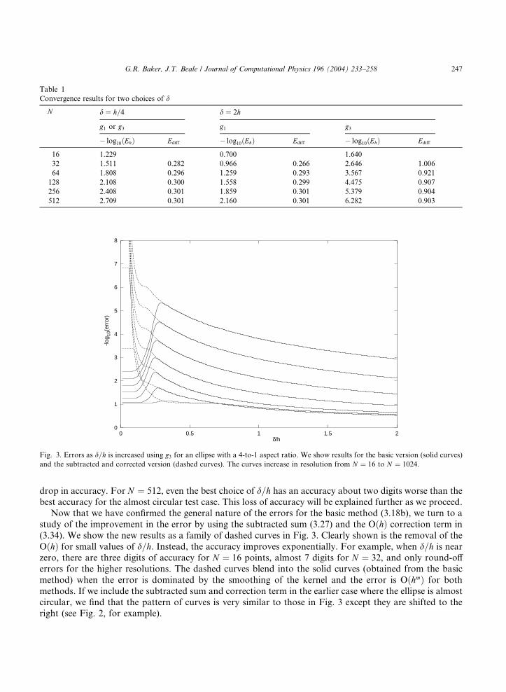
Table 1

Convergence results for two choices of d

N d ¼ h=4 d ¼ 2h

g1 or g3 g1 g3

� log10ðEhÞ Ediff � log10ðEhÞ Ediff � log10ðEhÞ Ediff

16 1.229 0.700 1.640

32 1.511 0.282 0.966 0.266 2.646 1.006

64 1.808 0.296 1.259 0.293 3.567 0.921

128 2.108 0.300 1.558 0.299 4.475 0.907

256 2.408 0.301 1.859 0.301 5.379 0.904

512 2.709 0.301 2.160 0.301 6.282 0.903

0

1

2

3

4

5

6

7

8

0 0.5 1 1.5 2δ/h

-log 1

0(er

ror)

Fig. 3. Errors as d=h is increased using g3 for an ellipse with a 4-to-1 aspect ratio. We show results for the basic version (solid curves)

and the subtracted and corrected version (dashed curves). The curves increase in resolution from N ¼ 16 to N ¼ 1024.


drop in accuracy. For N ¼ 512, even the best choice of d=h has an accuracy about two digits worse than the

best accuracy for the almost circular test case. This loss of accuracy will be explained further as we proceed.

Now that we have confirmed the general nature of the errors for the basic method (3.18b), we turn to a

study of the improvement in the error by using the subtracted sum (3.27) and the OðhÞ correction term in

(3.34). We show the new results as a family of dashed curves in Fig. 3. Clearly shown is the removal of the

OðhÞ for small values of d=h. Instead, the accuracy improves exponentially. For example, when d=h is near

zero, there are three digits of accuracy for N ¼ 16 points, almost 7 digits for N ¼ 32, and only round-offerrors for the higher resolutions. The dashed curves blend into the solid curves (obtained from the basic

method) when the error is dominated by the smoothing of the kernel and the error is OðhmÞ for both

methods. If we include the subtracted sum and correction term in the earlier case where the ellipse is almost

circular, we find that the pattern of curves is very similar to those in Fig. 3 except they are shifted to the

right (see Fig. 2, for example).


The reason for the shift in the graphs when the aspect ratio of the ellipse is increased lies in the local

spacing where the maximum error occurs. For the deformed ellipse, the maximum error always occurs near

n ¼ 0 (or n ¼ p). Since

s2n ¼ x2n þ y2n ¼ sin2 nþ a2 sinh2 r cos2 n; ð4:5Þ

the local spacing in arclength at n ¼ 0 is Ds ¼ snð0Þh ¼ h=4. If we pick d=h ¼ 0:3 where the uncorrected

results show a maximum, then d=ðDsÞ ¼ 1:2, a value consistent with the idea that d should be a little bigger

than the local spacing of the points. The implication is that all the curves in Fig. 3 would be stretched to the

right by a factor 4 if we used the local spacing snh instead of h as a scale for d.From these observations we are led to consider the smoothed kernel

Kdðn; n0Þ ¼ Kðn; n0Þf1þ gðqÞg with q ¼ jzðnÞ � zðn0ÞjdasnðnÞ

; ð4:6Þ

where da is constant. In other words, instead of specifying the blob size d in terms of the local spacing h in

the parametrization variable (d ¼ Ch), we will make the blob size proportional to the local spacing Ds ¼ snh(d ¼ CaDs ¼ Casnh ¼ dasn). In the first case, we pick C ¼ d=h, and in the second case, we pick Ca ¼ da=h. Are-examination of our error analysis indicates the conclusions are still valid if we replace d by dasn.

In Fig. 4 we show the results of varying da=h, rather than d=h for the same test cases as in Fig. 3, with or

without the subtraction and correction. As expected, the curves have been shifted to the right. At the same

time, there is a dramatic improvement in accuracy.The advantage of the adaptive d becomes clear when we consider the possible changes in the shape of the

interface during its motion. For example, suppose the vortex sheet were to start as a circle and then move

through the family of ellipses as though a were a simple function of time. This motion is not physical, of

course, since we are not moving the sheet with the correct velocity, but it does serve to give insight as to the

0

1

2

3

4

5

6

7

8

0 0.5 1 1.5 2δa/h

-log 1

0(er

ror)

Fig. 4. Errors with adjusted blob size as da=h is increased using g3 for a 4-to-1 ellipse. We show results for the basic version (solid

curves) and the subtracted and corrected version (dashed curves). The curves have resolution from N ¼ 16 to N ¼ 1024.


potential behavior of the error in the velocity. If we set d ¼ 2h, then as a increases we see a tremendous loss

of accuracy. With N ¼ 512, the errors for small times are about 10�6 (see Fig. 2). When a ¼ffiffiffiffiffi15

p=4, the

errors have increased to about 10�2 (see Fig. 4). On the other hand, if we set da ¼ 2h, then the initial error isthe same because sn ¼ 1, but when a ¼

ffiffiffiffiffi15

p=4 the errors will increase to 10�4 (see Fig. 4), a far more

reasonable increase. We confirm our speculations here in the next section when we consider the motion of

an interface during Rayleigh–Taylor instability.

Finally, we consider one more improvement. Even with the subtracted sum (3.27), the correction term

from (3.34), and the adjusted da, there is a steady drop-off in the accuracy as da=h increases. This suggests

we should replace g3 by g5 of (3.14c). There will be no change in the errors for small da=h (they remain

exponentially small), but there will be a noticeable improvement for large da=h from Oðh3Þ to Oðh5Þ. Inbetween where the corrected sum is still important, the errors should remain Oðh3Þ. The results, shown inFig. 5, support these estimates and, moreover, indicate a reasonable balance in the errors over the range of

da=h values. For da=h greater than about 1.2, the errors improve to Oðh5Þ, as evident from the spacing in the

curves for the larger values of N . For smaller values of da=h, the errors go through several changes in sign

where the spikes in the profiles should go to infinity, but they are truncated due to the frequency by which

the data points are plotted. Between da=h � 0:4 and � 1:0, the curves appear to be spaced by about 0.9,

indicating Oðh3Þ convergence. For even smaller values of da=h, spectral accuracy dominates.

This concludes our series of tests for closed vortex sheets. Next, we confirm that the same pattern of

behavior occurs for periodic sheets in open geometry. Here, we are not aware of a nontrivial test case, so weset the interface at xðnÞ ¼ nþ 0:5 sin n, yðnÞ ¼ 0:5 sin n, and pick the vortex sheet strength as

cðnÞ ¼ 1� 0:5 cos n. We then calculate the velocity with spectral accuracy by the alternate point quadrature

with N ¼ 512 points. Comparing with N ¼ 256, we conclude the errors are at the level of round-off.

Considering these results as ‘‘exact’’, we compute the errors as before; Eh ¼ maxj jqðnjÞ � qðhÞj j.

0

1

2

3

4

5

6

7

8

0 0.5 1 1.5 2δa/h

-log 1

0(er

ror)

Fig. 5. Errors using g5 with subtraction/correction as da=h is increased on the 4-to-1 ellipse. The curves increase from N ¼ 16 to

N ¼ 512 in powers in 2.

0

1

2

3

4

5

6

7

8

0 0.5 1 1.5 2δa/h

-log 1

0(er

ror)

Fig. 6. Errors using the closed form smooth periodic kernel with g5 and subtraction/correction as da=h is increased. The curves go from

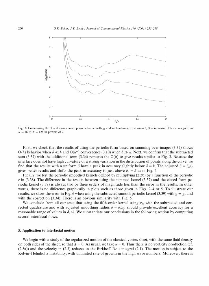
N ¼ 16 to N ¼ 128 in powers of 2.


First, we check that the results of using the periodic form based on summing over images (3.37) shows

OðhÞ behavior when d � h and OðhmÞ convergence (3.10) when d � h. Next, we confirm that the subtracted

sum (3.37) with the additional term (3.34) removes the OðhÞ to give results similar to Fig. 3. Because the

interface does not have high curvature or a strong variation in the distribution of points along the curve, we

find that the results with a uniform d have a peak in accuracy slightly below d ¼ h. The adjusted d ¼ dasngives better results and shifts the peak in accuracy to just above da ¼ h as in Fig. 4.

Finally, we test the periodic smoothed kernels defined by multiplying (2.2b) by a function of the periodicr in (3.38). The difference in the results between using the summed kernel (3.37) and the closed form pe-

riodic kernel (3.39) is always two or three orders of magnitude less than the error in the results. In other

words, there is no difference graphically in plots such as those given in Figs. 2–4 or 5. To illustrate our

results, we show the error in Fig. 6 when using the subtracted smooth periodic kernel (3.39) with g ¼ g5 andwith the correction (3.34). There is an obvious similarity with Fig. 5.

We conclude from all our tests that using the fifth-order kernel using g5, with the subtracted and cor-

rected quadrature and with adjusted smoothing radius d ¼ dasn, should provide excellent accuracy for a

reasonable range of values in da=h. We substantiate our conclusions in the following section by computingseveral interfacial flows.

5. Application to interfacial motion

We begin with a study of the regularized motion of the classical vortex sheet, with the same fluid density

on both sides of the sheet, so that A ¼ 0. As usual, we take a ¼ 0. Thus there is no vorticity production (cf.

(2.5a)) and the velocity in (2.3) reduces to the Birkhoff–Rott integral (2.1). The motion is subject to theKelvin–Helmholtz instability, with unlimited rate of growth in the high wave numbers. Moreover, there is


strong evidence, both analytic [15,17,34–36] and numerical [25,40] that a vortex sheet will develop curvature

singularities in finite time. For these reasons, it is natural to introduce a regularization to compute the

motion, as has been done in several studies. Krasny [26] explored thoroughly the effect of one regulari-zation. In the results presented here, we find results similar to Krasny�s for a first-order smoothed kernel,

but surprisingly different for the higher order kernels.

A typical initial condition for the study of the classical Kelvin–Helmholz instability is

xðnÞ ¼ n; yðnÞ ¼ 0; cðnÞ ¼ 1� e cos n: ð5:1Þ

With e ¼ 0:5, studies indicate that a curvature singularity forms at n ¼ p at time ts � 1:61. Rigorous

theory [18,33] establishes the existence of a weak solution for all time, when the vorticity has a distinguished

sign, but the precise nature of the solution is unknown. Moreover, the weak solution may not be unique.

One way that this weak solution can be determined is through the limiting behavior of smoothed kernels[29,33]. When the smoothed kernels satisfy certain properties, the limit d ! 0 will be a weak solution. One

of the conditions [29] is that the smoothed kernel is the convolution of the original kernel (2.2a) with a

radial blob function. The family (3.14) has this property. However, this condition may not be necessary; in

Krasny�s work with periodic vortex sheets [26], the regularization is not of this form, but the solutions

appear to have a weak limit [26]. Krasny�s regularization amounts to replacing r2, as defined in (3.38), by

r2 þ 2d2 in the denominator of the periodic velocity kernel. This can be thought of as a particular case of the

modification in (3.39) (without subtraction), where f ðr=dÞ ¼ r2=ðr2 þ 2d2Þ ¼ ðr=dÞ2=ððr=dÞ2 þ 2Þ. It is

reasonable to expect that the regularized periodic kernels of this sort also lead to a weak solution providedthe regularized vorticity is of one sign.

In Fig. 7 we compare a vortex sheet with Krasny�s regularization (dashed curve) to a similar one using

the first-order smoothed Gaussian kernel of (3.14a), with f ¼ 1þ g1 (solid curve). In Krasny�s case we taked ¼ 0:057, while for the Gaussian case d ¼ 0:1. We start at t ¼ 0 using (5.1) with e ¼ 0:5. We show a blow-

up of the vortex sheet near x ¼ p at t ¼ 3:0. In each case we use N points equally spaced in the parameter n

-0.2

-0.15

-0.1

-0.05

0

0.05

0.1

0.15

0.2

0.8 0.85 0.9 0.95 1 1.05 1.1 1.15 1.2x/π

y/π

Fig. 7. The roll-up of the vortex sheet using the first-order Gaussian kernel (solid curve) and Krasny�s regularization (dashed curve).


with N ¼ 512 and a time step of 0:0025 in a standard fourth-order Adams–Moulton predictor–corrector,

started with the standard fourth-order Runge–Kutta. Comparison with results of larger time steps and

lower resolutions indicate that the results are accurate to better than 10�8.We obtain the roll-up in Fig. 7 in the Gaussian case using either the periodic kernel from summing over

images (3.37) or the closed form periodic kernel (3.39): the maximum difference between the two profiles at

t ¼ 3:0 and with d ¼ 0:1 is less than 10�4. We do not bother with the correction terms since, in keeping with

common practice, we keep d fixed and increase N until good accuracy is achieved (d � h). The roll-up is

very similar to Krasny�s, but comparison is made difficult by the fact that our choice of d ¼ 0:1 has no

direct correspondence to his choices. A detailed comparison will be published elsewhere ([2]).

Next we present calculations of the same vortex sheet problem but regularized with the higher order

kernels. In Fig. 8, we show the result of using the third-order kernel with g3 from (3.14b). The initialcondition is again (5.1), and the sheet is shown at the same time t ¼ 3:0, with d ¼ 0:1 and 0:09. For d ¼ 0:1,we use a time step of 0:0025 and, to keep costs down, we start with N ¼ 512 points but double them when

the discrete Fourier spectrum is close to saturating (reaching k ¼ 256). Repeated doubling occurs at

t ¼ 1:5; 2:25; 2:5, the final resolution being N ¼ 4096. Also, we are forced to use a spectral filter introduced

by Krasny [25] to suppress the growth of round-off errors: Fourier amplitudes for x and y below 10�12 are

set to zero at the completion of each time step. For d ¼ 0:09, we use the same time step and double the

points at t ¼ 1:5; 2:25; 2:375; 2:75. Here, the filter level is 10�11.

Similarly, we show in Fig. 9 the results for the fifth-order kernel, with g5 in (3.14c), at t ¼ 3:0 and ford ¼ 0:2; 0:1. In both cases, we use a time step of 0:0025. For d ¼ 0:2, we start with N ¼ 512 and double

points at t ¼ 2:5. For d ¼ 0:1, we double points at t ¼ 1:5; 2:25; 2:5; 2:75; 2:875, ending with N ¼ 16384

points. The filter level must be set at 10�10.

The first observation is that the spirals are different from those obtained using a first-order kernel. The

main spiral is about the same size, but there is much more internal structure, and the appearance of new

smaller spirals on the outer arms. The third- and fifth-order kernels have strong similarities: compare

d ¼ 0:09 in the third-order kernel with d ¼ 0:1 in the fifth-order kernel. There is even some similarity in the

internal structures. The amazing detail appears even though the d�s are quite large. If we consider d as aneffective length scale for the smoothing, then the whole spiral falls inside a circle of radius d. Unfortunately,

we are unable to reduce d much more because of the computation time involved, and we must leave any

further study to another time. Nevertheless, the calculations indicate regularized vortex sheet motion with

the higher order kernels defined by (3.38), (3.39).

-0.2

-0.1

0

0.1

0.2

0.8 0.9 1 1.1 1.2

δ = 0.1

x/π

y/π

-0.2

-0.1

0

0.1

0.2

0.8 0.9 1 1.1 1.2

δ = 0.09

x/π

y/π

Fig. 8. Location of the vortex sheet – third-order kernel.

-0.2

-0.1

0

0.1

0.2

0.8 0.9 1 1.1 1.2

δ = 0.2

x/π

y/π

-0.2

-0.1

0

0.1

0.2

0.8 0.9 1 1.1 1.2

δ = 0.1

x/π

y/π

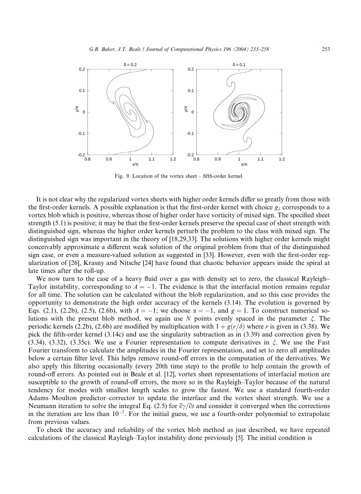
Fig. 9. Location of the vortex sheet – fifth-order kernel.


It is not clear why the regularized vortex sheets with higher order kernels differ so greatly from those withthe first-order kernels. A possible explanation is that the first-order kernel with choice g1 corresponds to a

vortex blob which is positive, whereas those of higher order have vorticity of mixed sign. The specified sheet

strength (5.1) is positive; it may be that the first-order kernels preserve the special case of sheet strength with

distinguished sign, whereas the higher order kernels perturb the problem to the class with mixed sign. The

distinguished sign was important in the theory of [18,29,33]. The solutions with higher order kernels might

conceivably approximate a different weak solution of the original problem from that of the distinguished

sign case, or even a measure-valued solution as suggested in [33]. However, even with the first-order reg-

ularization of [26], Krasny and Nitsche [24] have found that chaotic behavior appears inside the spiral atlate times after the roll-up.

We now turn to the case of a heavy fluid over a gas with density set to zero, the classical Rayleigh–

Taylor instability, corresponding to A ¼ �1. The evidence is that the interfacial motion remains regular

for all time. The solution can be calculated without the blob regularization, and so this case provides the

opportunity to demonstrate the high order accuracy of the kernels (3.14). The evolution is governed by

Eqs. (2.1), (2.2b), (2.5), (2.6b), with A ¼ �1; we choose a ¼ �1, and g ¼ 1. To construct numerical so-

lutions with the present blob method, we again use N points evenly spaced in the parameter n. The

periodic kernels (2.2b), (2.6b) are modified by multiplication with 1þ gðr=dÞ where r is given in (3.38). Wepick the fifth-order kernel (3.14c) and use the singularity subtraction as in (3.39) and correction given by

(3.34), (3.32), (3.35c). We use a Fourier representation to compute derivatives in n. We use the Fast

Fourier transform to calculate the amplitudes in the Fourier representation, and set to zero all amplitudes

below a certain filter level. This helps remove round-off errors in the computation of the derivatives. We

also apply this filtering occasionally (every 20th time step) to the profile to help contain the growth of

round-off errors. As pointed out in Beale et al. [12], vortex sheet representations of interfacial motion are

susceptible to the growth of round-off errors, the more so in the Rayleigh–Taylor because of the natural

tendency for modes with smallest length scales to grow the fastest. We use a standard fourth-orderAdams–Moulton predictor–corrector to update the interface and the vortex sheet strength. We use a

Neumann iteration to solve the integral Eq. (2.5) for oc=ot and consider it converged when the corrections

in the iteration are less than 10�7. For the initial guess, we use a fourth-order polynomial to extrapolate

from previous values.

To check the accuracy and reliability of the vortex blob method as just described, we have repeated

calculations of the classical Rayleigh–Taylor instability done previously [5]. The initial condition is


xðnÞ ¼ n; yðnÞ ¼ 0:5 cos n; cðnÞ ¼ 0: ð5:2Þ

We generate an ‘‘exact’’ solution by using the alternate point quadrature applied to the dipole version ofthe boundary integral technique as described in Baker et al. [6]. We start with N ¼ 64 and calculate up to

time t ¼ 1:6 with a time step of 0.0025. The filter level is set at 10�14 and the integral equation is considered

solved when successive iterates fall below 10�10 in absolute value. The calculation was stopped when the

Fourier amplitudes just below k ¼ 32 began to have values above the filter level. The number of points were

then doubled through interpolation based on the Fourier series, and the calculation continued to time 2.8

when the Fourier spectrum approached k ¼ 64. The filter level had to be raised to 10�13, and then raised

again to 10�10 to continue the calculations with N ¼ 256 points to time 3.8. The final doubling of points

allowed us to reach beyond time 4.0. We believe the results for this reference solution have an accuracy ofbetter than 10�8.

We ran the vortex blob codes in two cases, one with the blob size held fixed d ¼ 2h, and the other with

the adjusted blob size da ¼ 2h. We kept N fixed and ran as far as we could with the filter level set at 10�10 (as

was the convergence criteria for the solution of the integral equation). The time step was set at 0.0025. The

largest errors in the calculation occur near the tip of the spike at x ¼ p. For convenience, we compared the

tip of the spike with its ‘‘exact’’ location as an indicator of the error, even though this is a fairly severe

measure of the error. We show the results in Fig. 10 as two families of curves, corresponding to different

resolution N .The fifth-order accuracy is clearly observable in the errors in tip location. There is a continual degra-

dation in the accuracy as the spike grows. At early times, the spacing between the marker points is almost

uniform, and both families are close in accuracy. As the spike develops, the points cluster toward the tip

and the non-uniform spacing causes a significant difference in accuracy between the results for the fixed

blob size and the adjusted size. The results confirm that by adjusting d to the local spacing of the vortex

points we gain significant improvement in accuracy for vortex blob methods applied to interfacial motion.

0

1

2

3

4

5

6

7

8

0 0.5 1 1.5 2 2.5 3 3.5 4t

-log 1

0(er

ror)

Fig. 10. Errors in Rayleigh–Taylor flow, A ¼ �1, as a function of time for different resolutions, N ¼ 32; 64; 128; 256. The solid lines are

for the case d ¼ 2snh; the dashed lines are for the case d ¼ 2h.


We have confirmed the general pattern in the results for A > 0 (internal gravity waves) and, in particular,

A ¼ 1 (water waves). In our tests, we kept the amplitudes of the waves below that for which wave breaking

occurs, but large enough to see the effects of nonlinearity. Since the curvature remains moderate, the im-provement from adjusting the vortex blob with the local spacing is less dramatic than in Fig. 10.

Finally we turn to the remaining case of �1 < A < 0, with heavy fluid over light, for which the evolution

of the interface leads to the formation of a curvature singularity in finite time [4]. This case forces us to

consider the influence of the other terms in the equations of motion besides those involving the boundary

integrals. Simply smoothing the kernels in the integrals is not enough to avoid the onset of chaotic motion.

To obtain regular motion we also need to smooth terms involving the vortex sheet strength. One is the extra

term occurring in the velocity (2.3), which determines the tangential velocity of the markers,

a2

czn

¼ a2

csn

� �znsn

ð5:3aÞ

and other terms are in the evolution equation (2.5a) for c,

a2

�� A

4

�o

onc2

s2n

!þ Aa

csn

� �qn

znsn: ð5:3bÞ

The terms have been written to emphasize the (nonparametric) vortex sheet strength, c=sn. By smoothing

just this quantity in each of the terms above, we find that regularity is restored. If we neglected all the terms

in (2.3), (2.5a) but these, we would have a nonlinear hyperbolic system for xn, yn and c, which typically leads

to singularity formation in finite time. Thus it is reasonable to expect singularities to be suppressed bysmoothing these terms. (Tryggvason [43] also found that he needed to smooth the vortex sheet strength.)

We smooth the function c=sn in each occurrence in (5.3) using a blob regularization akin to that in the

velocity kernel. We use the smoothing, defined for a generic function f ,

fdðnÞ ¼1

dffiffiffip

pZ 1

�1f ðn0Þ exp

� jzðnÞ � zðn0Þj2

d2

!snðn0Þdn0: ð5:4Þ

We compute the integral directly with the trapezoidal rule. Because of the rapid decay of the exponential,we need use only a few points on either side of n, with jzðnÞ � zðn0Þj2 < 30d2. Since d will be much larger

than h, we do not use a discretization correction. The error in applying the filter will be Oðd2Þ. We can easily

improve (5.4) to higher order, but here we wish to establish success in regularizing the motion with the

simplest choice. Thus we use (5.4) and the first-order smoothing (3.14a) for the velocity integral, with the

same value of d in the two formulas. We again use the periodic velocity kernel in the form (3.39).

The choice of the parameter a affects the resolution of the calculation. An appealing physical choice is to

set a ¼ A, which picks the tangential velocity to be weighted with the densities. However, the resulting

motion crowds points away from the regions where resolution is needed, as observed by Kerr [23]. On theother hand, we find that the choice a ¼ 0 works well. There are several reasons why this may be so. First,

there is no clear choice for the tangential motion when regularization is used. Second, several of the

troublesome terms are removed with a ¼ 0; in (5.3), only the first term in (5.3b) remains. Third, the method

is more economical since derivatives of q are not needed. Finally, there is a simplification when f 7!fd is

applied to c=sn in that sn cancels.

We calculate the motion with two different values of A, starting with A ¼ �0:2, which corresponds to

fairly weak stratification. This case allows us to demonstrate the effectiveness of the method, since the

expected spiral forms. The initial condition is again (5.1) with e ¼ 0:5. In Fig. 11, we show the location ofthe interface at t ¼ 9:0 for three choices of d. Making use of symmetry, we show only half the periodic

interface for each choice. For d ¼ 0:4, 0.3, we used N ¼ 512 points and a time step of 0.0025. We applied

-5

-4

-3

-2

-1

0

1

2

3

4

0 0.5 1 1.5 2 2.5 3

δ = 0.4

-5

-4

-3

-2

-1

0

1

2

3

4

0 0.5 1 1.5 2 2.5 3

δ = 0.3

-5

-4

-3

-2

-1

0

1

2

3

4

0 0.5 1 1.5 2 2.5 3

δ = 0.2

Fig. 11. Location of the interface at time 9.0 with A ¼ �0:2 for three choices of d.


the Krasny Fourier filter with a cut-off level at 10�14 to maintain control over round-off errors. For d ¼ 0:2,we used N ¼ 512 up to t ¼ 6:5 then doubled the points, and doubled them again at t ¼ 8:0. The time step

was again 0.0025, but we raised the filter level to 10�12.

There is clear evidence of the formation of a spiral, but it becomes more difficult to resolve with de-

creasing d. The reason is the emergence of a drop of heavier fluid at the center, which is likely to be shed in

time. Unfortunately, the high curvature of the interface where the drop attaches to the spiral arms requires

higher and higher resolution, driving up the cost of the computations. Kerr [23] shows similar behavior for

A ¼ �0:1.In Fig. 12 we repeat the calculation with the Atwood ratio changed to A ¼ �0:5, so that the stratification

becomes strong. Now when the drop forms, it begins to detrain almost immediately, and there is an in-

dication of new drops forming on the arms. To get to the final time t ¼ 5:75, we started with N ¼ 512 points

and successively doubled the number when the tail of the spectrum reached N=2. For d ¼ 0:4, doublingoccurred at t ¼ 5:0; for d ¼ 0:3, at t ¼ 4:5; 5:375; and for d ¼ 0:2, at t ¼ 4:0; 4:625; 5:125. The Fourier filterlevel was set at 10�14 for the lower resolution runs and increased for the higher resolution runs but never

exceeded 10�12. The time step was 0.0025.

With Gaussian smoothed kernels we can see detailed structure in the spiral even with moderate size d. On

the other hand, convergence to a weak solution is less clear. In regions away from the spiral, we can seelinear convergence as d ! 0, in particular, at the lower tip of the falling spike. Inside the spiral, the vorticity

has mixed sign, and the emerging detail may be like that for the vortex sheet with A ¼ 0 and mixed sign

vorticity. As pointed out by Majda [33] for that case, it is possible that there is not a classical weak solution,

but rather one in a measure-valued sense. The results also show a scaling in time; that is, if the calculations

for d ¼ 0:4 or 0.3 are continued in time, the location of the sheet appears similar to that for d ¼ 0:2 at an

earlier time, although the size of the spiral is slightly larger.

In conclusion, we have demonstrated that high accuracy can be achieved with vortex blobs in the cal-

culation of two-dimensional interfacial flows where no curvature singularities arise, especially if the blobsize is adjusted to the local spacing. Further, we have identified the terms in the equations of motion for

-5

-4

-3

-2

-1

0

1

2

3

4

0 0.5 1 1.5 2 2.5 3

δ = 0.4

-5

-4

-3

-2

-1

0

1

2

3

4

0 0.5 1 1.5 2 2.5 3

δ = 0.3

-5

-4

-3

-2

-1

0

1

2

3

4

0 0.5 1 1.5 2 2.5 3

δ = 0.2

Fig. 12. Location of the interface at time 5.75 with A ¼ �0:5 for three choices of d.


general Atwood ratio that can lead to curvature singularities, and by smoothing them appropriately we can

calculate spiral formation. However, questions remain about the convergence as the blob size vanishes.

Finally, our approach has a natural extension to three-dimensional motion.

Acknowledgements

Research of the first author was supported by N.S.F. Grant DMS-0112759. Research of the second

author was supported by N.S.F. Grant DMS-0102356. We are indebted to Prof. Dan Meiron for several

useful discussions.

References

[1] C.R. Anderson, A vortex method for flows with slight density variations, J. Comput. Phys. 61 (1985) 417.

[2] G.R. Baker, L. Pham, in preparation.

[3] G.R. Baker, Generalized vortex methods for free-surface flows, in: R.E. Meyer (Ed.), Waves on Fluid Interfaces, Academic Press,

New York, 1983, p. 53.

[4] G.R. Baker, R.E. Caflisch, M. Siegel, Singularity formation during Rayleigh–Taylor instability, J. Fluid Mech. 252 (1993) 51.

[5] G.R. Baker, D.I. Meiron, S.A. Orszag, Vortex simulations of the Rayleigh–Taylor instability, Phys. Fluids 23 (1980) 1485.

[6] G.R. Baker, D.I. Meiron, S.A. Orszag, Generalized vortex methods for free-surface flow problems, J. Fluid Mech. 123 (1982) 477.

[7] G.R. Baker, D.I. Meiron, S.A. Orszag, Boundary integral methods for axisymmetric and three-dimensional Rayleigh–Taylor

instability problems, Physica D 12 (1984) 19.

[8] G.R. Baker, D.W. Moore, The rise and distortion of a two-dimensional gas bubble in an inviscid liquid, Phys. Fluids A 1 (1989)

1452.

[9] J.T. Beale, A grid-based boundary integral method for elliptic problems in 3D, SIAM J. Numer. Anal., 2003, accepted for

publication.

[10] J.T. Beale, M.-C. Lai, A method for computing nearly singular integrals, SIAM J. Numer. Anal. 38 (2001) 1902.

[11] J.T. Beale, A convergent boundary integral method for three-dimensional water waves, Math. Comput. 70 (2001) 977.


[12] J.T. Beale, T.Y. Hou, J.S. Lowengrub, Convergence of a boundary integral method for water waves, SIAM J. Numer. Anal. 33

(1996) 1797.

[13] J.T. Beale, A.J. Majda, High order accurate vortex methods with explicit velocity kernels, J. Comput. Phys. 58 (1985) 188.

[14] R.E. Caflisch, O.F. Orellana, Long time existence for a slightly perturbed vortex sheet, Commun. Pure Appl. Math. 39 (1986) 1.

[15] R.E. Caflisch, S. Semmes, A nonlinear approximation for vortex sheet evolution and singularity formation, Physica D 41 (1990)

197.

[16] A.J. Chorin, P. Bernard, Discretization of a vortex sheet with an example of roll-up, J. Comput. Phys. 13 (1973) 423.

[17] S.J. Cowley, G.R. Baker, S. Tanveer, On the formation of Moore curvature singularities in vortex sheets, J. Fluid Mech. 378

(1999) 233.

[18] J.-M. Delort, Existence de nappes de tourbillon en dimension deux, J. Am. Math. Soc. 4 (1991) 553.

[19] P.G. Drazin, W.H. Reid, Hydrodynamic Stability, Cambridge University Press, Cambridge, MA, 1981.

[20] J. Duchon, O. Robert, Global vortex-sheet solutions of Euler equations in the plane, J. Diff. Eqns. 73 (1988) 215.

[21] D.G. Ebin, Ill-posedness of the Rayleigh–Taylor and Helmholtz problems for incompressible fluids, Commun. Part. Diff. Eqns. 13

(1988) 1265.

[22] O. Hald, The convergence of vortex methods, II, SIAM J. Numer. Anal. 16 (1979) 726.

[23] R.M. Kerr, Simulation of Rayleigh–Taylor flows using vortex blobs, J. Comput. Phys. 76 (1988) 48.

[24] R. Krasny, M. Nitsche, The onset of chaos in vortex sheet flow, J. Fluid Mech. 454 (2002) 47.

[25] R. Krasny, A study of singularity formation in a vortex sheet by the point vortex method, J. Fluid Mech. 167 (1986) 65.

[26] R. Krasny, Desingularization of periodic vortex-sheet roll-up, J. Comput. Phys. 65 (1986) 292.

[27] K. Kuwahara, J. Takami, Numerical studies of two-dimensional vortex motion by a system of point vortices, J. Phys. Soc. Jpn. 34

(1973) 247.

[28] A. Leonard, Vortex methods for flow simulation, J. Comput. Phys. 37 (1980) 289.

[29] J.-G. Liu, Z. Xin, Convergence of vortex methods for weak solutions to the 2D Euler equations with vortex sheet data, Commun.

Pure Appl. Math. 48 (1995) 611.

[30] M.S. Longuet-Higgins, E.D. Cokelet, The deformation of steep surface waves on water, I. A numerical method of computation,

Proc. R. Soc. Lond. A 350 (1976) 1.

[31] T.S. Lundgren, N.N. Mansour, Oscillations of drops in zero gravity with weak viscous effects, J. Fluid Mech. 194 (1988) 479.

[32] A.J. Majda, A.L. Bertozzi, Vorticity and Incompressible Flow, Cambridge University Press, Cambridge, MA, 2002.

[33] A.J. Majda, Remarks on weak solutions for vortex sheets with a distinguished sign, Indiana Univ. Math. J. 42 (1993) 921.

[34] D.I. Meiron, G.R. Baker, S.A. Orszag, Analytic Structure of vortex sheet dynamics. I. Kelvin–Helmholtz instability, J. Fluid

Mech. 114 (1982) 283.

[35] D.W. Moore, The spontaneous appearance of a singularity in the shape of an evolving vortex sheet, Proc. R. Soc. Lond. A 365

(1979) 105.

[36] D.W. Moore, Numerical and analytical aspects of Helmholtz instability, in: Niordson, Olhoff (Eds.), Theoretical and Applied

Mechanics, Proceedings of XVI ICTAM, North-Holland, Amsterdam, 1985, p. 263.

[37] Q. Nie, G.R. Baker, Application of adaptive quadrature to axi-symmetric vortex-sheet motion, J. Comp. Phys. 143 (1998) 49.

[38] M. Nitsche, Axisymmetric vortex sheet motion: accurate evaluation of the principal value integral, SIAM J. Sci. Comput. 21

(1999) 1066.

[39] D.I. Pullin, Numerical studies of surface tension effects in nonlinear Kelvin–Helmholtz and Rayleigh–Taylor instability, J. Fluid

Mech. 119 (1982) 507.

[40] M.J. Shelley, A study of singularity formation in vortex-sheet motion by a spectrally accurate vortex method, J. Fluid Mech. 244

(1992) 493.

[41] A. Sidi, M. Israeli, Quadrature methods for periodic singular and weakly singular Fredholm integral equations, J. Sci. Comput. 3

(1988) 201.

[42] S. Tanveer, Singularities in the classical Rayleigh–Taylor flow: formation and subsequent motion, Proc. R. Soc. Lond. A 441

(1993) 501.

[43] G. Tryggvason, Numerical simulation of the Rayleigh–Taylor instability, J. Comput. Phys. 75 (1988) 253.

[44] W. Tsai, D. Yue, Computations of nonlinear free-surface flows, Ann. Rev. Fluid Mech. 28 (1996) 249.

[45] Y. Yang, The initial value problem of a rising bubble in a two-dimensional vertical channel, Phys. Fluids A 4 (1992) 913.

vortex blob methods applied to interfacial motionbeale/papers/baker.pdf · vortex blob methods...

Documents