Volatility, Valuation Ratios, and Bubbles: An

Empirical Measure of Market Sentiment

Can Gao Ian Martin∗

August, 2019

Abstract

We define a sentiment indicator based on option prices, valuation ratios

and interest rates. The indicator can be interpreted as a lower bound on

the expected growth in fundamentals that a rational investor would have

to perceive in order to be happy to hold the market. The lower bound was

unusually high in the late 1990s, reflecting dividend growth expectations

that in our view were unreasonably optimistic. We show that our measure

is a leading indicator of detrended volume, and of various other measures

associated with financial fragility. Our approach depends on two key ingre-

dients. First, we derive a new valuation-ratio decomposition that is related

to the Campbell and Shiller (1988) loglinearization, but which resembles

the Gordon growth model more closely and has certain other advantages.

Second, we introduce a volatility index that provides a lower bound on the

market’s expected log return.

∗Can Gao: Imperial College, London, http://www.imperial.ac.uk/people/can.gao14.

Ian Martin: London School of Economics, http://personal.lse.ac.uk/martiniw/. We thank

John Campbell, Stefan Nagel, Patrick Bolton, Ander Perez-Orive, Alan Moreira, Paul Schnei-

der, and seminar participants at Duke University and at the Federal Reserve Bank of New York

for their comments. Ian Martin is grateful to the ERC for support under Starting Grant 639744.

1

This paper introduces a market sentiment indicator that exploits two contrast-

ing views of market predictability.

A vast literature has studied the extent to which signals based on valuation

ratios are able to forecast market returns and/or measures of dividend growth;

early papers include Keim and Stambaugh (1986), Campbell and Shiller (1988),

and Fama and French (1988). More recently, Martin (2017) argued that indexes of

implied volatility based on option prices can serve as forecasts of expected excess

returns; and noted that the two classes of predictor variables made opposing

forecasts in the late 1990s, with valuation ratios pointing to low long-run returns

and option prices pointing to high short-run returns.

Our paper trades off the two views of the world against one other. Consider

the classic Gordon growth model, which relates the market’s dividend yield to

its expected return minus expected dividend growth: D/P = E(R − G). Very

loosely speaking, the idea behind the paper is to use option prices to measure ER,

and then to calculate the expected growth in fundamentals implicit in market

valuations—our sentiment measure—as the difference between the option price

index and dividend yield, EG = ER− E(R−G).

Putting this thought into practice is not as easy as it might seem, however. For

example, the Gordon growth model relies on assumptions that expected returns

and expected dividend growth are constant over time. The loglinearized identity

of Campbell and Shiller (1988) showed how to generalize the Gordon growth

model to the empirically relevant case in which these quantities are time-varying.

Their identity relates the price-dividend ratio of an asset to its expected future

log dividend growth and expected log returns. It is often characterized as saying

that high valuation ratios signal high expected dividend growth or low expected

returns (or both).

But expected returns are not the same as expected log returns. We show that

high valuations—and low expected log returns—may be consistent with high ex-

pected returns if log returns are highly volatile, right-skewed, or fat-tailed. Plau-

sibly, all of these conditions were satisfied in the late 1990s. As they are all

potential explanations for the rise in valuation ratios at that time, we will need

to be careful about the distinction between log returns and simple returns.

Furthermore, we show that while the Campbell–Shiller identity is highly ac-

2

curate on average, the linearization is most problematic at times when the price-

dividend ratio is far above its long-run mean. At such times—the late 1990s being

a leading example—a researcher who uses the Campbell–Shiller loglinearization

will conclude that long-run expected returns are even lower, and/or long-run ex-

pected dividend growth is even higher, than is actually the case.

We therefore propose a new linearization that does not have this feature, but

which also relates a measure of dividend yield to expected log returns and dividend

growth. Our approach exploits a measure of dividend yield yt = log (1 +Dt/Pt)

that has the advantage of being in “natural” units, unlike the quantity dpt =

logDt/Pt that features in the Campbell–Shiller approach. As a bonus, the re-

sulting identity bears a closer resemblance to the traditional Gordon growth

model—which it generalizes to allow for time-varying expected returns and divi-

dend growth—than does the Campbell–Shiller loglinearization.

The second ingredient of our paper is a lower bound on expected log returns.

(This plays the role of ER in the loose description above.) The lower bound

relies on an assumption closely related to the negative correlation condition of

Martin (2017); it can be computed directly from index option prices so is, broadly

speaking, a measure of implied volatility.

The paper is organized as follows. Section 1 discusses the link between val-

uation ratios, returns, and dividend growth; it analyzes the properties of the

Campbell–Shiller loglinearization, introduces our alternative loglinearization, and

studies the predictive relationship between the dividend yield measures and fu-

ture (log) returns and (log) dividend growth. Section 2 derives the lower bound

on expected returns. Section 3 combines the preceding sections to introduce the

sentiment indicator. Section 4 explores its relationship with volume and with

various other indicators of financial conditions. Section 5 concludes.

1 Fundamentals

We seek to exploit the information in valuation ratios, following Campbell and

Shiller (1988). We write Pt+1, Dt+1 and Rt+1 for the level, dividend, and gross

3

return of the market, respectively: thus

Rt+1 =Dt+1 + Pt+1

Pt. (1)

It follows from (1) that

rt+1 − gt+1 = pdt+1 − pdt + log(1 + edpt+1

), (2)

where we write dpt+1 = dt+1− pt+1 = logDt+1− logPt+1, pdt+1 = pt+1− dt+1, and

gt+1 = dt+1 − dt. Campbell and Shiller (1988) linearized the final term in (2) to

derive a decomposition of the (log) price-dividend ratio,1

pdt =k

1− ρ+∞∑i=0

ρi Et (gt+1+i − rt+1+i) , (3)

where the constants k and ρ are determined by

ρ =µ

1 + µand

k

1− ρ= (1 + µ) log(1 + µ)− µ log µ , where µ = epd.

The approximation (3) is often loosely summarized by saying that high val-

uation ratios signal high expected dividend growth or low expected returns (or

both). But expected log returns are not the same as expected returns:2 we have

Et rt+1+i = logEtRt+1+i −1

2vart rt+1+i −

∞∑n=3

κ(n)t (rt+1+i)

n!,

where κ(n)t (rt+1+i) is the nth conditional cumulant of the log return. (If returns

are conditionally lognormal, then the higher cumulants κ(n)t (rt+1+i) are zero for

n ≥ 3.) Thus high valuations—and low expected log returns—may be consistent

1We follow the convention in the literature in writing approximations such as (3) with equalssigns. A number of our results below are in fact exact. We emphasize these as they occur.We also assume throughout the paper that there are no rational bubbles, as is standard in theliterature. Thus, for example, in deriving (3) we are assuming that limT→∞ ρT pdT = 0.

2And expected log dividend growth is not the same as expected dividend growth. Thisdistinction is less important, however, as log dividend growth is less volatile than log returns.

4

with high expected arithmetic returns if log returns are highly volatile, right-

skewed, or fat-tailed. Plausibly, all of these conditions were satisfied in the late

1990s. As they are all potential explanations for the rise in valuation ratios at

that time,3 we will need to be careful about the distinction between log returns

and simple returns.

Furthermore, the Campbell–Shiller first-order approximation is least accurate

when the valuation ratio is far from its mean, as we now show.

Result 1 (Campbell–Shiller revisited). The log price-dividend ratio pdt obeys the

following exact decomposition:

pdt =k

1− ρ+∞∑i=0

ρi (gt+1+i − rt+1+i)+1

2

∞∑i=0

ρiψt+1+i(1−ψt+1+i)(pdt+1+i − pd

)2,

(4)

where the constants k and ρ are defined as above, and the quantities ψt+1+i lie

between ρ and 1/(1 + edpt+1+i).

Equation (4) becomes a second-order Taylor approximation if ψt is assumed

equal to ρ for all t,

pdt =k

1− ρ+∞∑i=0

ρi (gt+1+i − rt+1+i) +ρ(1− ρ)

2

∞∑i=0

ρi(pdt+1+i − pd

)2, (5)

and reduces to the Campbell–Shiller loglinearization (3) if the final term on the

right-hand side of (4) is neglected entirely.

Proof. Taylor’s theorem, with the Lagrange form of the remainder, states that

(for any sufficiently well-behaved function f , and for x ∈ R and a ∈ R)

f(x) = f(a) + (x− a)f ′(a) +1

2(x− a)2 f ′′(ξ) , for some ξ between a and x. (6)

We apply this result with f(x) = log (1 + ex), x = dpt+1, and a = dp = E dptequal to the mean log dividend yield. Equation (6) becomes

log(1 + edpt+1

)= k + (1− ρ)dpt+1 +

1

2ψt+1(1− ψt+1)

(dpt+1 − dp

)2,

3See, for example, Pastor and Veronesi (2003, 2006).

5

where ψt+1 = 1/(1 + eξ) must lie between 1/(1 + edp) = ρ and 1/(1 + edpt+1).

Substituting into expression (2), we have the exact relationship

rt+1 − gt+1 = k − pdt + ρpdt+1 +1

2ψt+1(1− ψt+1)

(pdt+1 − pd

)2which can be solved forward to give the result (4). The approximation (5) follows.

Result 1 expresses the price-dividend ratio in terms of future log dividend

growth and future log returns—as in the Campbell–Shiller approximation—plus

a convexity correction.

This convexity correction is small on average. Take the unconditional expec-

tation of second-order approximation (5):

E pdt =k

1− ρ+

E (gt − rt)1− ρ

+ρ

2var pdt ,

assuming that pdt, rt, and gt are stationary so that their unconditional means

and variances are well defined. Using CRSP data from 1947 to 2017, the sample

average of pdt is 3.483 (so that ρ is 0.970) and the sample standard deviation

is 0.436. Thus the unconditional average convexity correction ρ2

var pdt is about

0.0924, that is, about 2.65% of the size of E pdt.The convexity correction can be large conditionally, however. We have

pdt =k

1− ρ+∞∑i=0

ρi Et (gt+1+i − rt+1+i) +ρ(1− ρ)

2

∞∑i=0

ρi Et(pdt+1+i − pd

)2,

and the final term may be quantitatively important if the valuation ratio is far

from its mean and persistent, so that it is expected to remain far from its mean

for a significant length of time.

For the sake of argument, suppose the log price-dividend ratio follows an

AR(1), pdt+1 − pd = φ(pdt − pd) + εt+1, where vart εt+1 = σ2 so that var pdt =

σ2/(1−φ2); and set σ = 0.168 and φ = 0.923 to match the sample standard devi-

ation and autocorrelation in CRSP data from 1947–2017. The above expression

6

becomes

pdt =k

1− ρ+∞∑i=0

ρi Et (gt+1+i − rt+1+i) +ρ(1− ρ)φ2

2(1− ρφ2)

[(pdt − pd

)2+

σ2

(1− ρ)φ2

]︸ ︷︷ ︸

convexity correction

.

At its peak during the boom of the late 1990s, pdt was 2.2 standard deviations

above its mean. The convexity term then equals 0.145: this is the amount by

which a researcher using the Campbell–Shiller approximation would overstate∑∞i=0 ρ

i Et (gt+1+i − rt+1+i). With ρ = 0.970, this is equivalent to overstating

Et gt+1+i− rt+1+i by 14.5 percentage points for one year, 3.1 percentage points for

five years, or 1.0 percentage points for 20 years.4

The Campbell–Shiller approximation does not apply if dpt follows a random

walk (i.e., Et dpt+1 = dpt). But in that case we can linearize (2) around the

conditional mean Et dpt+1 to find5

Et (rt+1 − gt+1) = log(1 + edpt

)= log

(1 +

Dt

Pt

). (7)

Motivated by this fact,6 we define yt = log (1 +Dt/Pt). An appealing property

of this definition—and one that dpt does not possess—is that yt = log(1+Dt/Pt) ≈Dt/Pt. We can then rewrite the definition of the log return (2) as the (exact)

relationship

rt+1 − gt+1 = yt + log(1− e−yt

)− log

(1− e−yt+1

). (8)

4The numbers are more dramatic if we use the long sample from 1871–2015 available onRobert Shiller’s website. We find ρ = 0.960, σ = 0.136, and φ = 0.942 in the long sample, sothat the convexity correction is 0.0596 when pdt is at its mean, and 0.253 at the peak (whichwas 3.2 standard deviations above the mean). This last number corresponds to overstatingEt gt+1+i − rt+1+i by 25.3 percentage points for one year, 5.5 percentage points for five years,1.8 percentage points for 20 years, or 1.0 percentage points for ever.

5Campbell (2008, 2018) derives the same result via a different route, but makes furtherassumptions (that the driving shocks are homoskedastic and conditionally Normal) that we donot require.

6As further motivation, this measure of dividend yield also emerges naturally in i.i.d. modelswith power utility or Epstein–Zin preferences, as shown by Martin (2013).

7

In these terms, equation (7) states that

yt = Et (rt+1 − gt+1) , (9)

which is valid, as a first-order approximation, if dpt (or yt) follows a random walk.

Alternatively, if yt is stationary (as is almost always assumed in the literature)

we have the following result. We write unconditional means as y = E yt, r = E rtand g = E gt.

Result 2 (A variant of the Gordon growth model). We have the loglinearization

yt = (1− ρ)∞∑i=0

ρi (rt+1+i − gt+1+i) , (10)

where7 ρ = e−y. As there is no constant in (10), and as (1− ρ)∑∞

i=0 ρi = 1, this

is a variant of the Gordon growth model: y is a weighted average of future r − g.

To second order, we have the approximation

yt = (1− ρ)∞∑i=0

ρi (rt+1+i − gt+1+i)−1

2

ρ

1− ρ

∞∑i=0

ρi[(yt+1+i − y)2 − (yt+i − y)2

].

(11)

We also have the exact relationship

y = r − g, (12)

which does not rely on any approximation.

Proof. Using Taylor’s theorem to second order in equation (8), we have the second-

order approximation

rt+1 − gt+1 =1

1− ρyt −

ρ

1− ρyt+1 +

1

2

ρ

(1− ρ)2[(yt+1 − y)2 − (yt − y)2

]7This differs slightly from the definition of ρ in Result 1, though they are extremely close in

practice.

8

which can be rewritten

yt = (1− ρ)(rt+1 − gt+1) + ρyt+1 −1

2

ρ

1− ρ[(yt+1 − y)2 − (yt − y)2

],

and then solved forward, giving (10) and (11). Equation (12) follows by taking ex-

pectations of the identity (8) and noting that E log (1− e−yt) = E log (1− e−yt+1)

by stationarity of yt.

We note in passing that equation (12) implies that r > g in any model in

which yt is stationary. Piketty (2015) writes that “the inequality r > g holds true

in the steady-state equilibrium of the most common economic models, including

representative-agent models where each individual owns an equal share of the

capital stock.” Our result shows that the inequality applies much more generally

and does not rely on equilibrium logic.

Given our focus on bubbles, we are particularly interested in the accuracy

of these loglinearizations at times when valuation ratios are unusually high or,

equivalently, when dpt and yt are unusually low. This motivates the following

definition and result.

Definition 1. We say that yt is far from its mean (at time t) if

Et[(yt+1+i − y)2

]≤ (yt − y)2 for all i ≥ 0. (13)

Example.—If yt follows an AR(1), then a direct calculation shows that yt is far

from its mean if and only if it is at least one standard deviation from its mean.

Result 3 (Signing the approximation errors). We can sign the approximation

error in the Campbell–Shiller loglinearization (3):

dpt < −k

1− ρ+∞∑i=0

ρi Et (rt+1+i − gt+1+i) . (14)

The first-order approximation (10) is exact on average. That is,

E yt = (1− ρ)∞∑i=0

ρi E (rt+1+i − gt+1+i) (15)

9

holds exactly, without any approximation. But if yt is far from its mean then (up

to a second-order approximation)

yt ≥ (1− ρ)∞∑i=0

ρi Et (rt+1+i − gt+1+i) . (16)

Proof. The inequality (14) follows immediately from (4) and equation (15) follows

directly from equation (12). To establish the inequality (16), rewrite

∞∑i=0

ρi[(yt+1+i − y)2 − (yt+i − y)2

]= − (yt − y)2 + (1− ρ)

∞∑i=0

ρi (yt+1+i − y)2

= (1− ρ)∞∑i=0

ρi[(yt+1+i − y)2 − (yt − y)2

].

(17)

The inequality then follows from (11), (13), and (17).

Dividend yields, whether measured by dpt or by yt, were unusually low around

the turn of the millennium, indicating some combination of low future returns

and high future dividend growth. Result 3 shows that an econometrician who

uses the Campbell–Shiller approximation (3) at such a time—that is, who treats

the inequality (14) as an equality—will overstate how low future returns, or how

high future dividend growth, must be: and therefore may be too quick to con-

clude that the market is “bubbly.” In contrast, an econometrician who uses the

approximation (10) will understate how low future returns, or how high future

dividend growth, must be. Thus yt is a conservative diagnostic for bubbles.

To place more structure on the relationship between valuation ratios and r

and g, we will make an assumption about the evolution of dpt and yt over time.

For now we will rely on an AR(1) assumption to keep things simple; in Section

3.1, we report the corresponding results assuming AR(2) or AR(3) processes.

The Campbell–Shiller approximation over one period states that rt+1− gt+1 =

k+dpt−ρ dpt+1. If dpt follows an AR(1) with autocorrelation φ then Et dpt+1−dp =

φ(dpt − dp

), so

Et (rt+1 − gt+1) = c+ (1− ρφ)dpt, (18)

10

RHSt

yt

dpt

LHSt+1

rt+1 − gt+1

rt+1

−gt+1

rt+1 − gt+1

rt+1

−gt+1

a0 s.e. a1 s.e. R2

−0.067 [0.049] 3.415 [1.317] 7.73%

−0.018 [0.050] 3.713 [1.215] 10.51%

−0.049 [0.028] −0.298 [0.812] 0.32%

0.417 [0.146] 0.107 [0.042] 7.58%

0.500 [0.138] 0.114 [0.041] 9.92%

−0.083 [0.085] −0.007 [0.024] 0.19%

Table 1: Full-sample regressions for S&P 500, annual data, cash reinvestment,1947–2017.

where we have absorbed constant terms into c.

Conversely, the first-order approximation underlying Result 2 implies that

Et (rt+1 − gt+1) =1

1− ρyt −

ρ

1− ρEt yt+1. (19)

If yt follows an AR(1) with autocorrelation φy then this reduces to

Et (rt+1 − gt+1) = c+1− ρφy1− ρ

yt, (20)

where again we absorb constants into the intercept c. In view of (12), this can

also be written without an intercept as

Et (rt+1 − gt+1)− (r − g) =1− ρφy1− ρ

(yt − y) ,

so that the deviation of yt from its long-run mean is proportional to the deviation

of conditionally expected rt+1− gt+1 from its long-run mean. A further advantage

of yt over dpt is that the expression (20) is also meaningful if yt follows a random

walk: in this case, the coefficient on yt equals one and the intercept is zero, by

equation (9).

Equations (18) and (20) motivate regressions of realized rt+1 − gt+1 onto dpt

and a constant, or onto yt and a constant. The results are shown in Table 1,

11

where we also report the results of regressing rt+1 and −gt+1 separately onto yt

and onto dpt. We use end-of-year observations of the price level and accumulated

dividends of the S&P 500 index from CRSP.8 The table reports regression results

in the form

LHSt+1 = a0 + a1 × RHSt + εt+1,

with Hansen–Hodrick standard errors. (Under the AR(1) assumption, we could

also use (18) or (20) as estimates of Et(rt+1 − gt+1). This approach turns out to

give very similar results, as we show in Table 11 of the appendix.)

The variables yt and dpt have similar predictive performance and, consistent

with the prior literature, we find, in the post-1947 sample, that valuation ratios

help to forecast returns but have limited forecasting power for dividend growth.

Table 2 reports results using cash reinvested dividends in the post-1926 period,

which is the longest sample CRSP has. Tables 3 and 4 report similar results using

semi-annual data. Tables 5 to 8 report results using the NYSE value-weighted

index price and dividend data and compare them with market reinvested S&P500

data. Table 9 uses the price and dividend data of Goyal and Welch (2008) (up-

dated to 2017 and taken from Amit Goyal’s webpage): this gives us a longer

sample, as it incorporates Robert Shiller’s data which goes back as far as 1871.

The predictability of r relative to g is to some extent a feature of the post-war pe-

riod. In the long sample, returns are substantially less predictable and dividends

substantially more predictable, perhaps because of the post-war tendency of cor-

porations to smooth dividends (Lintner, 1956). Encouragingly, though, we find

that the predictive relationship between yt (or dpt) and the difference rt+1 − gt+1

is fairly stable across sample periods and data sources.

8We calculate the monthly dividend by multiplying the difference between monthly cum-dividend and ex-dividend returns by the lagged ex-dividend price: Dt = (Rcum,t − Rex,t)Pt−1.As we aggregate the dividends paid out over the year, to address seasonality issues, we reinvestdividends month-by-month until the end of the year, using the CRSP 30-day T-bill rate as ourrisk-free rate. In the appendix, we report similar results with dividends reinvested at the cum-dividend market return rather than at a risk-free rate; if anything, these results are somewhatmore favorable to our yt variable than to dpt.

12

2 A lower bound on expected log returns

High valuation ratios are sometimes cited as direct evidence of a bubble. But

valuation ratios can be high for good reasons if interest rates or rationally expected

risk premia are low. In other words, if we use yt to measure Et (rt+1 − gt+1) as

suggested above, we may find that yt is low simply because Et rt+1 is very low,

which could reflect low interest rates rf,t+1, low (log) risk premia Et rt+1 − rf,t+1,

or both.

While interest rates are directly observable, risk premia are harder to measure.

We start from the following identity, which generalizes an identity introduced by

Martin (2017) in the case Xt+1 = Rt+1:

EtXt+1 =1

Rf,t+1

E∗t (Rt+1Xt+1)− covt (Mt+1Rt+1, Xt+1) .

We have written E∗t for the time-t conditional risk-neutral expectation operator,

defined by the property that 1Rf,t+1

E∗t Xt+1 = Et (Mt+1Xt+1), where Mt+1 denotes

a stochastic discount factor that prices any tradable payoff Xt+1 received at time

t+1. Assuming the absence of arbitrage, such an SDF must exist, and the identity

above holds for any gross return Rt+1 such that the payoff Rt+1Xt+1 is tradable.

Henceforth, however, Rt+1 will always denote the gross return on the market.

We are interested in expected log returns, Xt+1 = logRt+1, in which case the

identity becomes

Et logRt+1 =1

Rf,t+1

E∗t (Rt+1 logRt+1)− covt (Mt+1Rt+1, logRt+1) . (21)

The first of the two terms on the right-hand side, as a risk-neutral expectation,

is directly observable from asset prices, as it represents the price of a contract that

pays Rt+1 logRt+1 at time t+ 1. (Neuberger (2012) has studied this contract in a

different context.) The second term can be controlled: we will argue below that

it is reasonable to impose an assumption that it is negative. Thus (21) implies

a lower bound on expected log returns in terms of a quantity that is directly

observable from asset prices.

To make further progress, we make two assumptions throughout the paper.

13

As we will see below, we will use option prices to bound the first term on the

right-hand side of the identity (21). Our first assumption addresses the minor9

technical issue that we observe options on the ex-dividend value of the index, Pt+1,

rather than on Pt+1 +Dt+1.

Assumption 1. If we define the dispersion measure Ψ(Xt+1) ≡ E∗t f(Xt+1) −f(E∗t Xt+1), where f(x) = x log x is a convex function, then the dispersion of Rt+1

is at least as large as that of Pt+1/Pt:

Ψ (Rt+1) ≥ Ψ (Pt+1/Pt) . (22)

This condition is very mild. Expanding f(x) = x log x as a Taylor series to

second order around x = 1, f(x) ≈ (x2−1)/2. Thus, to second order, Assumption

1 is equivalent to var∗t Rt+1 ≥ var∗t (Pt+1/Pt), or equivalently var∗t (Pt+1 +Dt+1) ≥var∗t Pt+1. A sufficient, though not necessary, condition for this to hold is that

the price Pt+1 and dividend Dt+1 are weakly positively correlated under the risk-

neutral measure.

Our second assumption is more substantive.

Assumption 2. The modified negative correlation condition holds:

covt (Mt+1Rt+1, logRt+1) ≤ 0 . (23)

Martin (2017) imposed the closely related negative correlation condition (NCC)

that covt (Mt+1Rt+1, Rt+1) ≤ 0. The two conditions are equivalent in the lognor-

mal case, as we show below, and more generally the two are plausible for similar

reasons: in any reasonable model, Mt+1 will be negatively correlated with the

return on the market, Rt+1, and we know from the bound of Hansen and Ja-

gannathan (1991), coupled with the empirical fact that high Sharpe ratios are

9In fact, it is so minor that the distinction between options on Pt+1 and options on Pt+1 +Dt+1 is often neglected entirely in the literature. For example, Neuberger (2012) “avoid[s]irrelevant complications with interest rates and dividends” by treating options on forward pricesas observable, as do Schneider and Trojani (2018), and (essentially equivalently) Carr and Wu(2009) use options on stocks as proxies for options on stock futures. These authors effectivelyassume that our inequality (22) holds with equality.

14

available, that Mt+1 is highly volatile. The following two examples are adapted

from Martin (2017).

Example 1.—Suppose that the SDF Mt+1 and return Rt+1 are condition-

ally jointly lognormal and write rf,t+1 = logRf,t+1, µt = logEtRt+1, and σ2t =

vart logRt+1. Then the modified NCC is equivalent to the assumption that the

conditional Sharpe ratio of the asset, λt ≡ (µt− rf,t+1)/σt, exceeds its conditional

volatility, σt; and hence also to the original NCC, covt(Mt+1Rt+1, Rt+1) ≤ 0.

Proof. By Stein’s lemma, covt (Mt+1Rt+1, logRt+1) = covt (logMt+1 + logRt+1, logRt+1).

By lognormality of Mt+1 and Rt+1, the fact that Et (Mt+1Rt+1) = 1 is equiv-

alent to logEtMt+1 + logEtRt+1 = − covt (logMt+1, logRt+1). It follows from

these two facts that covt (Mt+1Rt+1, logRt+1) ≤ 0 if and only if vart logRt+1 ≤logEtRt+1 − rf,t+1: that is, if and only if λt ≥ σt. This condition is equivalent to

covt(Mt+1Rt+1, Rt+1) ≤ 0 in the lognormal case, as shown by Martin (2017).

The Sharpe ratio of the market is typically thought of as being on the order

of 30–50%, while the volatility of the market is on the order of 16–20%. Thus the

modified NCC holds in the calibrated models of Campbell and Cochrane (1999),

Bansal and Yaron (2004), Bansal et al. (2014) and Campbell et al. (2016), among

many others.

We include the above example because the lognormality assumption is com-

monly imposed. But Martin (2017) argues that option prices are inconsistent

with the assumption. This motivates our second example, which does not require

lognormality.

Example 2.—Suppose that there is an unconstrained investor who maximizes

expected utility over next-period wealth, who chooses to invest his or her wealth

fully in the stock market, and whose relative risk aversion (which need not be

constant) is at least one at all levels of wealth. Then the modified NCC holds for

the market return.

Proof. The given conditions imply that the SDF is proportional (with a constant

of proportionality that is known at time t) to u′(WtRt+1). We must therefore

show that covt(u′(WtRt+1)Rt+1, logRt+1) ≤ 0. This holds for the very strong

reason—much stronger than is actually needed for the NCC or modified NCC to

15

hold—that u′(WtRt+1)Rt+1 is decreasing in Rt+1: its derivative is u′(WtRt+1) +

WtRt+1u′′(WtRt+1) = −u′(WtRt+1) [γ(WtRt+1)− 1], which is negative because rel-

ative risk aversion γ(x) ≡ −xu′′(x)/u′(x) is at least one.

We can now state our lower bound on expected log returns.

Result 4. Suppose Assumptions 1 and 2 hold. Write callt(K) and putt(K) for

the time t prices of call and put options on Pt+1 with strike K, and Ft for the time

t forward price of the index for settlement at time t+ 1. Then we have

Et rt+1 − rf,t+1 ≥1

Pt

{∫ Ft

0

putt(K)

KdK +

∫ ∞Ft

callt(K)

KdK

}︸ ︷︷ ︸

LVIXt

. (24)

Proof. As E∗t Rt+1 = Rf,t+1 and E∗t Pt+1 = Ft, the inequality (22) can be rear-

ranged as

1

Rf,t+1

E∗t Rt+1 logRt+1 − logRf,t+1 ≥1

Rf,t+1

[E∗t(Pt+1

Ptlog

Pt+1

Pt

)− FtPt

logFtPt

].

(25)

The right-hand side of this inequality can be measured directly from option

prices using a result of Breeden and Litzenberger (1978) that can be rewritten, fol-

lowing Carr and Madan (2001), to give, for any sufficiently well behaved function

g(·),

1

Rf,t+1

[E∗t g(Pt+1)− g(E∗t Pt+1)] =

∫ Ft

0

g′′(K) putt(K) dK+

∫ ∞Ft

g′′(K) callt(K) dK.

Setting g(x) = xPt

log xPt

, we have g′′(x) = 1/(Ptx). Thus

1

Rf,t+1

[E∗t(Pt+1

Ptlog

Pt+1

Pt

)− FtPt

logFtPt

]=

1

Pt

{∫ Ft

0

putt(K)

KdK +

∫ ∞Ft

callt(K)

KdK

}.

(26)

The result follows on combining the identity (21), the inequalities (23) and

(25), and equation (26).

We refer to the right-hand side of equation (24) as LVIX because it is reminis-

16

cent of the definition of the VIX index which, in our notation, is

VIX2t = 2Rf,t+1

{∫ Ft

0

putt(K)

K2dK +

∫ ∞Ft

callt(K)

K2dK

},

and of the SVIX index introduced by Martin (2017),

SVIX2t =

2

Rf,t+1P 2t

{∫ Ft

0

putt(K) dK +

∫ ∞Ft

callt(K) dK

}.

We do not annualize our definition (24), so to avoid unnecessary clutter we have

also not annualized the definitions of VIX and SVIX above. We will typically

choose the period length from t to t + 1 to be six or 12 months. The forecasting

horizon dictates the maturity of the options, so for example we use options expiring

in 12 months to measure expectations of 12-month log returns.

VIX, SVIX, and LVIX place differing weights on option prices. VIX has a

weighting function 1/K2 on the prices of options with strike K; LVIX has weight-

ing function 1/K; and SVIX has a constant weighting function. In this sense

we can think of LVIX as lying half way between VIX and SVIX. (We could also

introduce a factor of two into the definition of LVIX to make the indices look even

more similar to one another, but have chosen not to.)

We calculate LVIX using end-of-month interest rates and S&P 500 index option

prices from OptionMetrics. In practice, we do not observe option prices at all

strikes between zero and infinity, so we have to truncate the integral on the right-

hand side of (24) (as does the CBOE in its calculation of the VIX index). In doing

so, we understate the idealized value of the integral. That is, our lower bound

would be even higher if given perfect data: it is therefore conservative.

Figure 1 plots LVIXt over our sample period from January 1996 to December

2017.

2.1 Empirical evidence on the modified NCC

We have motivated the inequality of Result 4 via a theoretical argument that the

modified NCC should hold. In this section, we assess the inequality empirically.

Specifically, we examine the realized forecast errors rt+1 − rf,t+1 − LVIXt in

17

2000 2005 2010 20150.00

0.02

0.04

0.06

0.08

1 month 3 months 6 months 12 months

Figure 1: The LVIX index, which provides a lower bound on the market’s expectedexcess log return (Et rt+1 − rf,t+1), by Result 4.

order to carry out a one-sided t-test of the hypothesis that the inequality (24)

fails. With standard errors computed using a block bootstrap,10 we find a p-value

of 0.097. Thus despite our relatively short sample period—which is imposed on

us by the availability of option price data—we can reject the hypothesis with

moderate confidence. This supports our approach.

More optimistically, it is natural to wonder whether the inequality (24) might

approximately hold with equality (though we emphasize that this does not need

to be the case for our approach to make sense). For this to be the case, we would

need both (22) and (23) to hold with approximate equality. As the conditional

volatility of dividends is substantially lower than that of prices, it is reasonable

to think that this is indeed the case for (22), and as noted in footnote 9, much

of the literature implicitly makes that assumption. Meanwhile the modified NCC

(23) would hold with equality if (but not only if) one thinks from the perspective

of an investor with log utility who chooses to hold the market, as is clear from

the proof provided in Example 2 above. The perspective of such an investor has

been shown to provide a useful benchmark for forecasting returns on the stock

10As our sample is 276 months long, we use a block length of seven months, following theT 1/3 rule of thumb for block length for a sample of length T . For comparison, the correspondingp-value using naive OLS standard errors would be 0.001.

18

market (Martin, 2017), on individual stocks (Martin and Wagner, 2019), and on

currencies (Kremens and Martin, 2019).

Table 10 in the Appendix reports the results of running the regression

rt+1 − rf,t+1 = α + β × LVIXt + εt+1 (27)

at horizons of 3, 6, 9, and 12 months. Returns are computed by compounding

the CRSP monthly gross return of the S&P 500. We report Hansen–Hodrick

standard errors to allow for heteroskedasticity and autocorrelation that arises due

to overlapping observations. If the inequality (24) holds with equality, we should

find α = 0 and β = 1. We do not reject this hypothesis at any horizon; and

at the six- and nine-month horizons we can reject the hypothesis that β = 0 at

conventional significance levels.

3 A sentiment indicator

We can now put the pieces together. We will measure expectations about funda-

mentals by subtracting Et (rt+1 − gt+1), as revealed by valuation ratios under our

AR(1) assumption, from Et rt+1, as revealed by interest rates and option prices:

Et gt+1 = rf,t+1 + Et (rt+1 − rf,t+1)− Et (rt+1 − gt+1)

≥ rf,t+1 + LVIXt − Et (rt+1 − gt+1) . (28)

The inequality follows (under our maintained Assumptions 1 and 2) because

Et rt+1 − rf,t+1 ≥ LVIXt, as shown in Result 4.

We refer to the lower bound as the sentiment indicator, Bt. Our central

definition uses yt to measure Et(rt+1 − gt+1) via the fitted value a0 + a1yt, as

in Table 1, giving

Bt = rf,t+1 +1

Pt

[∫ Ft

0

putt(K)

KdK +

∫ ∞Ft

callt(K)

KdK

]− (a0 + a1yt) .

We estimate the coefficients a0 and a1 using an expanding window: for example, at

time t they are estimated using data from 1947 until time t. Thus Bt is observable

19

2000 2005 2010 20150.00

0.05

0.10

0.15

Bt Bdp,t

(a) Full sample.

2000 2005 2010 20150.00

0.05

0.10

0.15

Bt Bdp,t

(b) Real time.

Figure 2: The bubble indicator, computed using an expanding window to estimatethe relationship between yt and rt+1 − gt+1 (left) or using the full sample (right).

at time t. If one thinks in terms of Example 2, above, to motivate the modified

NCC, then Bt is a lower bound on the expected dividend growth Et gt+1 that must

be perceived by an investor who has risk aversion higher than 1 and who is happy

to hold the market.

If Et gt+1 itself follows an AR(1)—as in the work of Bansal and Yaron (2004)

and many others—then Bt can also be interpreted, after rescaling, as a lower

bound on long-run dividend expectations. For if we have Et+1 gt+2−g = φg (Et gt+1 − g)+

εg,t+1 then long-run expected dividend growth at time t is

(1− ρ)∑i≥0

ρi (Et gt+1+i − g) =1− ρ

1− ρφg(Et gt+1 − g) ,

where we have introduced a factor 1 − ρ in the definition of long-run expected

dividend growth so that the weights (1 − ρ)ρi sum to 1 and long-run expected

dividend growth can be interpreted as a weighted average of all future periods’

expected growth.

Figure 2a plots Bt over our sample period using the full sample from 1947 to

2017 to estimate the relationship between yt (or dpt) and rt+1 − gt+1. We work

at an annual horizon, so that the value of Bt at a given point in time is (subject

to our maintained assumptions) a lower bound on the expected dividend growth

20

2000 2005 2010 2015

-0.04

-0.02

0.00

0.02

0.04

0.06

0.08

r f ,t+1 LVIXt Et[gt+1-rt+1]

Figure 3: The three components of the sentiment indicator.

over the subsequent year. Figure 2b shows the corresponding results using using

an expanding window to estimate the relationship, so that the resulting series is

observable in real time. Encouragingly, the indicator behaves stably as we move

from full-sample information to real-time information. Unless otherwise indicated,

we will henceforth work with the series that is observable in real time.

The figures also show modified indicators, Bdp,t, that use dpt rather than yt to

measure Et (rt+1 − gt+1), as in (18). These have the advantage of familiarity—dpt

has been widely used in the literature—but the disadvantage that they may err

on the side of signalling a bubble too soon, as shown in Result 3. Consistent with

this prediction, the two series line up fairly closely, but the Bdp,t series are less

conservative—in that they suggest even higher Et gt+1—during the period in the

late 1990s when valuation ratios were far from their mean.

Note, moreover, that net dividend growth satisfies Et Dt+1

Dt− 1 > Et gt+1,

because egt+1 − 1 > gt+1. Thus our lower bound on expected log dividend

growth implies still higher expected arithmetic dividend growth. If dividend

growth were conditionally lognormal, for example, we would have logEt Dt+1

Dt=

Et gt+1 + 12

vart gt+1. The variance term is small unconditionally—in our sample

period, var gt+1 ≈ 0.005—but it is plausible that during the late 1990s there was

unusually high uncertainty about log dividend growth.

21

Figure 3 plots the three components of the sentiment indicator Bt from 1996

to 2017. LVIX and Et(gt+1 − rt+1) moved in opposite directions for most of our

sample period, with high valuation ratios occurring at times of low risk premia.

But all three components were above their mean during the late 1990s.

It might seem strange that we rely on asset prices to provide a rational lower

bound on expected log returns (via Result 4) while simultaneously arguing that

the market itself was mispriced during part of our sample period. To sharpen the

point, consider, for the sake of argument, the special case discussed in Section 2.1.

Our volatility measure LVIX then directly measures the expected excess log return

perceived by a log investor who chooses to hold the market.

Yet we simultaneously claim that there was a bubble in the late 1990s. These

positions may appear to be inconsistent—why would a rational investor hold an

overvalued stock market?—but they are not. The loglinearized identity yt =

(1−ρ)∑∞

i=0 ρi (rt+1+i − gt+1+i) shows that one can simultaneously have high short-

run expected log returns Etrt+1, high valuation ratios—i.e., low yt—and make

rational forecasts of fundamentals∑∞

i=0 ρi Et gt+1+i, so long as future expected

returns∑

i>0 ρi Et rt+1+i are low. And, critically, the log investor does not care

about expected returns in future: he or she is myopic, so can be induced to hold

the market by high short-run returns Et rt+1 whatever his or her beliefs about

subsequent expected returns.

But something has to give. For the investor to perceive high expected log

returns and, simultaneously, low expected log dividend growth during the bubble

period, he or she must have believed that the historical forecasting relationship

between dividend yield and Et (rt+1 − gt+1) had broken down.

To see this, write Et(rt+1 − gt+1) for the regression-implied time-t forecast of

rt+1 − gt+1, which may differ from the agent’s rational forecast Et (rt+1 − gt+1).

Then, from inequality (28), we have

Et gt+1 = rf,t+1 + Et (rt+1 − rf,t+1)− Et (rt+1 − gt+1) +[Et (rt+1 − gt+1)− Et (rt+1 − gt+1)

]≥ rf,t+1 + LVIXt − a0 − a1yt︸ ︷︷ ︸

Bt

+[Et (rt+1 − gt+1)− Et (rt+1 − gt+1)

].

An agent who believed, in the late 1990s, that Et gt+1 was lower than Bt must

22

therefore have concluded that Et (rt+1 − gt+1) < Et (rt+1 − gt+1). By the loglin-

earization (19), this is equivalent to Et yt+1 < Et yt+1.

Such an agent’s beliefs were therefore consistent only if she expected yt+1 to

remain, in the short run, lower—and valuations higher—than suggested by the

historical evidence. This possibility is consistent with the findings of Brunnermeier

and Nagel (2004), who argued that in the late 1990s sophisticated investors such as

hedge funds positioned themselves to exploit high short-run returns despite being

skeptical about longer run returns, and with the view of the world colorfully

articulated by former Citigroup chief executive Chuck Prince in a July, 2007,

interview with the Financial Times : “When the music stops, in terms of liquidity,

things will be complicated. But as long as the music is playing, you’ve got to get

up and dance. We’re still dancing.”

3.1 Alternative stochastic processes for yt

We have modelled yt as following an AR(1) to avoid overfitting. Aside from

the obvious advantages of parsimony, the partial autocorrelations of yt, shown in

Figure 8 of Appendix C, support this choice: the partial autocorrelations of yt at

lags greater than one are close to zero.

The question of how to model yt is not central to the point of this paper,

however, so we also consider the possibility that yt follows an AR(2) or AR(3).11

If yt follows an AR(2) process, then from the linearization (19) we have

rt+1 − gt+1 = α + βyt + γyt−1 + εt+1,

while if yt follows an AR(3) process, then

rt+1 − gt+1 = α + βyt + γyt−1 + δyt−2 + εt+1.

The results of these regressions are reported in Table 12 of Appendix C.

11Alternatively, our approach could easily accommodate, say, a vector autoregression for yt;the key is that one has an empirical procedure that is not prone to overfitting and that generatesa sensible measure of Et yt+1 to be used in (19).

23

2000 2005 2010 2015-0.05

0.00

0.05

0.10

AR(1) AR(2) AR(3)

(a) Full sample.

2000 2005 2010 2015-0.02

0.00

0.02

0.04

0.06

0.08

0.10

0.12

AR(1) AR(2) AR(3)

(b) Real time.

Figure 4: Bubble indicators calculated on a full-sample or real-time basis, assum-ing yt follows an AR(1), AR(2) or AR(3) process.

The corresponding lower bounds on Et gt+1 are shown in Figure 4.12 They are

very similar to our baseline measure during the late 1990s, but they are lower

during the crisis of 2008–9 and higher in its immediate aftermath. Once again,

we note that the indicator behaves fairly stably as we move from full-sample

information to real-time information.

3.2 Variations

3.2.1 What if the valuation ratio follows a random walk?

A true believer in the New Economy might have argued that our measure of

Et (rt+1 − gt+1), which is based on an assumption that yt follows an AR(1)—or

AR(2) or AR(3)—had broken down during the late 1990s. Perhaps the most

aggressive possibility one could reasonably entertain is the “random walk” view

that the price-dividend ratio had ceased to mean-revert entirely, as considered by

Campbell (2008, 2018). This perspective might also be adopted by a cautious

central banker to justify inaction on the basis that valuation ratios could remain

very high indefinitely.

12These lower bounds are rely on regressions using expanding windows, so are observable inreal time, like our baseline measure. Figure 4a, in Appendix C, shows the corresponding indexesusing the full sample to estimate the AR processes.

24

2000 2005 2010 2015

0.00

0.02

0.04

0.06

0.08

Bt

Figure 5: The alternative sentiment indicator, Bt.

We now show how to accommodate this possibility by defining a closely related

bubble index that was also high in the late 1990s. If yt follows a random walk

then, from equation (9),

Et gt+1(9)= Et rt+1 − yt ≥ LVIXt + rf,t − yt︸ ︷︷ ︸

Bt

,

where we define a variant on our previous indicator,

Bt = LVIXt + rf,t − yt , (29)

that has the further benefit of not requiring estimation of any free parameters.

More generally, if all one knows is that Et yt+1 ≥ yt—irrespective of the details

of the evolution of yt—then equation (19) implies that we have

Et gt+1 ≥ Bt .

Figure 5 shows the time series of Bt. Even if valuation ratios were expected to

follow a random walk in the late 1990s—a dubious proposition in any case—the

implied expectations about cashflow growth appear implausibly high.

Unlike our preferred indicator, Bt, the random walk version Bt spiked almost as

high during the subprime crisis as it did around the turn of the millennium. This

25

reflects the fact that implied volatility, and hence the LVIX index, rose dramat-

ically during the last months of 2008, indicating that log returns were expected

to be very high over the subsequent year (by Result 4). From the perspective

of our notional policymaker who believed that valuation ratios follow a random

walk, these high expected log returns could only have reflected high expected

log dividend growth. This prediction is unreasonable, in our view, because the

random walk assumption is unreasonable. The point is that even a policymaker

who believed valuation ratios followed a random walk would have had to perceive

unusually high expected dividend growth in the late 1990s.

3.2.2 What if dividend growth is unforecastable?

If dividend growth is unforecastable, as in the work of Campbell and Cochrane

(1999) and many others, then valuation ratios reveal long-run expectations of log

returns while LVIX reveals the corresponding short-run expectations.

Specifically, if dividend growth is unforecastable and yt is stationary, then from

equation (10)

yt = (1−ρ)∞∑i=0

ρi Et [rt+1+i − gt+1+i] = (1−ρ)Et[rt+1]+(1−ρ)ρ∞∑i=0

ρi Et[rt+2+i]−g.

This equation can be rearranged to give

Et rt+1 − (1− ρ)∑i≥0

ρi Et rt+2+i =Et rt+1 − yt − g

ρ.

Finally, we can exploit the inequality Et rt+1−rf,t ≥ LVIXt of Result 4 to conclude

that

Et rt+1︸ ︷︷ ︸short-run returns

− (1− ρ)∑i≥0

ρi Et rt+2+i︸ ︷︷ ︸long-run returns

≥ LVIXt + rf,t − yt − gρ

=Bt − gρ

.

This inequality provides an alternative interpretation of the indicator Bt =

LVIXt + rf,t − yt that we defined in equation (29) above, and which is plotted in

26

2000 2005 2010 20150.00

0.02

0.04

0.06

0.08

0.10

0.12

0.14

linear quadratic cubic

(a) Full sample.

2000 2005 2010 2015-0.3

-0.2

-0.1

0.0

0.1

0.2

0.3

linear quadratic cubic

(b) Real time.

Figure 6: Bubble indicators calculated with linear, quadratic, and cubic specifi-cations for the relationship between expected rt+1 − gt+1 and yt.

Figure 5. If dividend growth is unforecastable, unusually high levels of Bt indicate

that short-run expected log returns are unusually high relative to subsequent long-

run expected log returns.

3.2.3 Nonlinearity in the functional form

We can also allow for a nonlinear relationship between rt+1 − gt+1 and yt. In

Appendix D, we report the results of running regressions of the form

rt+1 − gt+1 = a0 + a1yt + a2y2t + εt+1

and

rt+1 − gt+1 = a0 + a1yt + a2y2t + a3y

3t + εt+1.

Figure 6a shows that these regressions deliver very similar results to the linear

specification reported above when we use the full sample period to estimate the

coefficients ai. But the coefficient estimates in the higher order specifications are

strikingly unstable when we estimate the regressions in real time using expanding

windows (Figure 6b), even though the regressions are estimated on almost 50

years of data at the start of our sample period, that is, on data from 1947 to 1996.

In the late 1990s, for example, the estimated cubic specification implies a

27

negative relationship between yt and forecast rt+1−gt+1 around the then prevailing

value of yt. That is, given the then recent association of unusually low dividend

yield with high realized returns, the cubic specification predicts extremely high

returns going forward, as shown in Figure 9a, Appendix D. (It is important that

the low dividend yields at the time were unusual, because the cubic specification

makes it possible to associate high returns with extremely low yields without

materially altering the long established relationship between low returns and low

yields that prevails over the usual range of yields.)

We view this exercise as a cautionary tale. Given that bubbles occur fairly

rarely, it is particularly important to avoid the possibility that an (over-)elaborate

model achieves superior performance in-sample by overfitting the historical data.

The ingredients of a bubble indicator should behave stably during historically

unusual periods, as our simple linear specification does (Figure 9b, Appendix D).

4 Other indicators of financial conditions

We now compare the sentiment indicator to some other indicators of financial

conditions that have been proposed in the literature.

4.1 Volume

We start by exploring the relationship with volume, which has been widely pro-

posed as a signature of bubbles (see, for example, Harrison and Kreps, 1978;

Duffie, Garleanu and Pedersen, 2002; Cochrane, 2003; Lamont and Thaler, 2003;

Ofek and Richardson, 2003; Scheinkman and Xiong, 2003; Hong, Scheinkman and

Xiong, 2006; Barberis et al., 2018). We construct a daily measure of volume using

Compustat data from January 1983 to December 2017, by summing the product

of shares traded and daily low price over all S&P 500 stocks on each day. (We find

essentially identical results if we use daily high prices to construct the measure.)

As volume trended strongly upward during our sample period, we subtract a lin-

ear trend from log volume. We do so on using an expanding window, so that our

detrended log volume measure, which we call vt, is (like Bt) observable at time t.

Figure 7a plots detrended log volume, vt, and Bt over the sample period, with

28

both series standardized to zero mean and unit variance. There is a remarkable

similarity between the two series, so it is worth emphasizing that they are each

based on entirely different input data. The sentiment index is a leading indicator

of volume: Figure 7b plots the correlation between (detrended) volume at time t,

vt, and the sentiment index at time t + k, where k is measured in months. The

shaded area indicates a bootstrapped13 95% confidence interval. The correlation

between the two peaks at more than 90% for k around −10 months. Figure 10,

in the appendix, leads to the same conclusion using full-sample, as opposed to

real-time, information to compute both Bt and the detrended volume measure.

4.2 The probability of a crash

One expects that the probability of a crash should be higher during a bubble

episode; if not, the episode is perhaps not actually a bubble.14 We use a measure

of the probability of a crash derived by Martin (2017, Result 2) that can be

computed in terms of option prices:

P (Rt+1 < α) = α

[put′t(αPt)−

putt(αPt)

αPt

](30)

where put′t(K) is the first derivative of put price as a function of strike, evaluated

at K. This represents the probability of a market decline perceived by a log

investor who holds the market. The probability of a crash (30) is high when out-

of-the-money put prices are highly convex, as a function of strike, at strikes at

and below αPt. By contrast, the measure of volatility (24) that is relevant for our

sentiment indicator is a function of option prices across the full range of strikes of

out-of-the-money puts and calls.

Figure 7c plots the crash probability over time. The probability of a crash was

elevated during the late 1990s, consistent with standard intuition about bubbles.

13Each k defines an original sample of size Nk. We draw 10,000 bootstrap samples of size Nk

by sampling from the original sample with replacement, and compute the correlation coefficientin each case, then use the 2.5 and 97.5 percentiles to define the edges of the confidence interval.We use the same procedure in the correlation plots shown in Figures 7, 10b, and 11.

14Greenwood, Shleifer and You (2018) document, at the industry level, that sharp increasesin stock prices do indeed signal a heightened probability of a crash.

29

2000 2005 2010 2015

-1

0

1

2

Bt vt

(a) Bt and detrended volume.

-30 -20 -10 0 10 20 30k

0.4

0.5

0.6

0.7

0.8

0.9

corr(Bt+k,vt)

(b) Correlation between Bt+k and volume.

2000 2005 2010 20150.00

0.05

0.10

0.15

Bt Prob of -20% in 6 months

(c) Bt and crash probability.

-30 -20 -10 10 20 30k

-0.4

-0.2

0.2

0.4

0.6corr(Bt+k,Pt)

(d) Correlation between Bt+k and crashprobability.

Figure 7: The sentiment indicator, volume and crash probability. Shaded areasin the right-hand panels indicate bootstrapped 95% confidence intervals.

30

But it was also high in the aftermath of the subprime crisis, an episode that we

would certainly not identify as bubbly. Figure 7d plots the correlation between

the two series at different leads and lags. The sentiment measure is a leading

indicator of crash probability at horizons of about two years. The correlation flips

sign for positive values of k, indicating that there is a tendency for the sentiment

indicator to be high following periods in which the crash probability is low.

4.3 Other measures

In the interest of completeness, we report results for various other measures of

financial conditions in Appendix E. The panels of Figure 11 explore the relation-

ship between the bubble index and three other measures of financial conditions:

the excess bond premium (EBP) of Gilchrist and Zakrajsek (2012), and the Na-

tional Financial Conditions Index (NFCI) and Adjusted National Financial Con-

ditions Index (ANFCI) generated on a weekly basis by the Federal Reserve Bank

of Chicago (converted to monthly data by taking the last week’s observation in

each calendar month).

Finally, Table 14 reports the correlations between Bt and various other senti-

ment measures, together with p-values that indicate that each of the correlations

is significantly different from zero; and Figures 12 and 13 plot the corresponding

time series. We have relegated these to the end because we only have incomplete

sample periods for the measures in question (2000:Q2 to 2017:Q4 in the case of the

Graham–Harvey series, and 2003:Q1 to 2015:Q3 for the De la O–Myers series).

In particular, all the series are missing what is, from our point of view, the most

interesting period around and before the turn of the millennium.

Specifically, ER1yr and ER10yr are, respectively, the cross-sectional average

subjective expectations stock market returns over 1- and 10-year horizons, as

reported by respondents to the surveys studied by Ben-David, Graham and Harvey

(2013); EER1yr and EER10yr are the corresponding average subjective expected

excess returns; and ERstd1yr and ERstd10yr are disagreement measures at the

same horizons (that is, are the cross-sectional standard deviations of reported

subjective expected returns). Lastly, DM survey indicates a time series of average

subjective expectations of dividend growth that has been constructed by De la O

31

and Myers (2018).

The measures of mean subjective expected returns, and of mean subjective

expected dividend growth, are positively correlated with Bt, while the measures

of mean subjective expected excess returns, and of disagreement, are negatively

correlated with Bt.

5 Conclusion

We have presented a sentiment indicator based on interest rates, index option

prices, and the market valuation ratio. The indicator can be interpreted in various

ways; perhaps the simplest is as a lower bound on the expected dividend growth

that must be perceived by an investor who (i) is rational, (ii) has relative risk

aversion at least one, and (iii) is happy to invest his or her wealth fully in the

stock market.

The bound was very high during the late 1990s, reflecting dividend growth

expectations that in our view were unreasonably optimistic—hence our description

of it as a sentiment indicator—and that were not realized ex post. We also show

that it is a leading indicator of detrended volume and of various measures of stress

in the financial system.

In simple terms, we characterize the late 1990s as a bubble because valuation

ratios and short-run expected returns—as revealed by interest rates and our LVIX

measure—were simultaneously high. Both aspects are important. We would not

view high valuation ratios at a time of low expected returns, or low valuation ratios

at a time of high expected returns, as indicative of a bubble: on the contrary, the

latter scenario occurs in the aftermath of the market crash in 2008.

Our measure does not point to an unreasonable level of market sentiment in

recent years, as it interprets high valuation ratios as being justified by the low level

of interest rates and implied volatility. A skeptic might respond that the low level

of implied volatility is in itself indicative of unreasonable complacency. This is,

in principle, a possibility. In the terminology of Shiller (2000), we are measuring

“bubble expectations” rather than “confidence.” Valuation ratios, interest rates

and volatility could be internally consistent in our sense—so that our measure

would not signal that anything is amiss—while also being mispriced. The measure

32

should be viewed as a test of the internal coherence of valuation ratios, interest

rates, and option prices, rather than as a panacea.

Our approach also requires an appeal to the good judgment of policymakers:

we have not addressed the hard question of how to identify whether a given level

of expected dividend growth is reasonable. More generally, our hope is that the

indicator might become one of several inputs into the policy decision process,

rather than becoming the basis for a deterministic rule for action. We do not

see a way to avoid some degree of expert judgment in identifying market-wide

bubbles; but we do believe that the approach proposed in this paper would make

it easier for such judgment to be applied in a focussed and disciplined manner.

Volatility and valuation ratios have, of course, long been linked to bubbles. A

novel feature of our approach is that we use some theory to motivate our definitions

of volatility and of valuation ratios, and to make the link quantitative. Our

approach also satisfies the requirement noted by Brunnermeier and Oehmke (2013)

that practically useful risk measures should be “measurable in a timely fashion.”

There are various choices to be made regarding the details of the construction of

the indicator: we have tried to make these choices in a conservative way to avoid

“crying bubble” prematurely, in the hope that the indicator might be useful to

cautious policymakers in practice.

References

Bansal, Ravi, and Amir Yaron. 2004. “Risks for the Long Run: A PotentialResolution of Asset Pricing Puzzles.” Journal of Finance, 59(4): 1481–1509.

Bansal, Ravi, Dana Kiku, Ivan Shaliastovich, and Amir Yaron.2014. “Volatility, the Macroeconomy, and Asset Prices.” Journal of Finance,69(6): 2471–2511.

Barberis, Nicholas, Robin Greenwood, Lawrence Jin, and AndreiShleifer. 2018. “Extrapolation and Bubbles.” Journal of Financial Economics,129: 203–227.

Ben-David, Itzhak, John R. Graham, and Campbell R. Harvey. 2013.“Managerial Miscalibration.” Quarterly Journal of Economics, 128(4): 1547–1584.

33

Breeden, Douglas T., and Robert H. Litzenberger. 1978. “Prices of State-Contingent Claims Implicit in Option Prices.” Journal of Business, 51(4): 621–651.

Brunnermeier, Markus K., and Martin Oehmke. 2013. “Bubbles, FinancialCrises, and Systemic Risk.” In Handbook of the Economics of Finance. Vol. 2B,, ed. George M. Constantinides, Milton Harris and Rene M. Stulz, 1221–1288.Amsterdam:Elsevier North Holland.

Brunnermeier, Markus K., and Stefan Nagel. 2004. “Hedge Funds and theTechnology Bubble.” Journal of Finance, 59(5): 2013–2040.

Campbell, John Y. 2008. “Viewpoint: Estimating the Equity Premium.” Cana-dian Journal of Economics, 41(1): 1–21.

Campbell, John Y. 2018. Financial Decisions and Markets: A Course in AssetPricing. Princeton University Press.

Campbell, John Y., and John H. Cochrane. 1999. “By Force of Habit: AConsumption-Based Explanation of Aggregate Stock Market Behavior.” Jour-nal of Political Economy, 107(2): 205–251.

Campbell, John Y., and Robert J. Shiller. 1988. “The Dividend-Price Ra-tio and Expectations of Future Dividends and Discount Factors.” Review ofFinancial Studies, 1: 195–228.

Campbell, John Y., Stefano Giglio, Christopher Polk, and Robert Tur-ley. 2016. “An Intertemporal CAPM with Stochastic Volatility.” Working Pa-per.

Carr, Peter, and Dilip Madan. 2001. “Towards a Theory of Volatility Trad-ing.” In Option Pricing, Interest Rates and Risk Management. Handbooks inMathematical Finance, , ed. E. Jouini, J. Cvitanic and Marek Musiela, 458–476. Cambridge University Press.

Carr, Peter, and Liuren Wu. 2009. “Variance Risk Premiums.” Review ofFinancial Studies, 22(3): 1311–1341.

Cochrane, John H. 2003. “Stocks as Money: Convenience Yield and the Tech-Stock Bubble.” In Asset Price Bubbles. , ed. William C. Hunter, George G.Kaufman and Michael Pomerleano. Cambridge:MIT Press.

De la O, Ricardo, and Sean Myers. 2018. “Subjective Cash Flow and DiscountRate Expectations.” Working paper, Stanford University.

34

Duffie, Darrell, Nicolae Garleanu, and Lasse H. Pedersen. 2002. “Securi-ties Lending, Shorting, and Pricing.” Journal of Financial Economics, 66: 307–339.

Fama, Eugene F., and Kenneth R. French. 1988. “Dividend Yields andExpected Stock Returns.” Journal of Financial Economics, 22(1): 3–25.

Gilchrist, Simon, and Egon Zakrajsek. 2012. “Credit Spreads and BusinessCycle Fluctuations.” American Economic Review, 102(4): 1692–1720.

Goyal, Amit, and Ivo Welch. 2008. “A Comprehensive Look at the Empiri-cal Performance of Equity Premium Prediction.” Review of Financial Studies,21: 1455–1508.

Greenwood, Robin, Andrei Shleifer, and Yang You. 2018. “Bubbles forFama.” Journal of Financial Economics. forthcoming.

Hansen, Lars Peter, and Ravi Jagannathan. 1991. “Implications of SecurityMarket Data for Models of Dynamic Economies.” Journal of Political Economy,99(2): 225–262.

Harrison, J. Michael, and David M. Kreps. 1978. “Speculative Investor Be-havior in a Stock Market with Heterogeneous Expectations.” Quarterly Journalof Economics, 92(2): 323–336.

Hong, Harrison, Jose Scheinkman, and Wei Xiong. 2006. “Asset Float andSpeculative Bubbles.” Journal of Finance, 61(3): 1073–1117.

Keim, Donald B., and Robert F. Stambaugh. 1986. “Predicting Returns inthe Stock and Bond Markets.” Journal of Financial Economics, 17: 357–390.

Kremens, Lukas, and Ian Martin. 2019. “The Quanto Theory of ExchangeRates.” American Economic Review, 109(3): 810–843.

Lamont, Owen A., and Richard H. Thaler. 2003. “Can the Market Add andSubtract? Mispricing in Tech Stock Carve-Outs.” Journal of Political Economy,111(2): 227–268.

Lintner, John. 1956. “Distribution of Incomes of Corporations Among Divi-dends, Retained Earnings, and Taxes.” American Economic Review Papers &Proceedings, 46: 97–113.

Martin, Ian. 2013. “Consumption-Based Asset Pricing with Higher Cumulants.”Review of Economic Studies, 80(2): 745–773.

35

Martin, Ian. 2017. “What is the Expected Return on the Market?” QuarterlyJournal of Economics, 132(1): 367–433.

Martin, Ian W. R., and Christian Wagner. 2019. “What is the ExpectedReturn on a Stock?” Journal of Finance, 74(4): 1887–1929.

Neuberger, Anthony. 2012. “Realized Skewness.” Review of Financial Studies,25(11): 3423–3455.

Ofek, Eli, and Matthew Richardson. 2003. “DotCom Mania: The Rise andFall of Internet Stock Prices.” Journal of Finance, 58(3): 1113–1137.

Pastor, Lubos, and Pietro Veronesi. 2003. “Stock Valuation and Learningabout Profitability.” Journal of Finance, 58(5): 1749–1789.

Pastor, Lubos, and Pietro Veronesi. 2006. “Was there a Nasdaq bubble inthe late 1990s?” Journal of Financial Economics, 81: 61–100.

Piketty, Thomas. 2015. “About Capital in the Twenty-First Century.” Ameri-can Economic Review: Papers & Proceedings, 105(5): 48–53.

Scheinkman, Jose A., and Wei Xiong. 2003. “Overconfidence and SpeculativeBubbles.” Journal of Political Economy, 111(6): 1183–1219.

Schneider, Paul, and Fabio Trojani. 2018. “(Almost) Model-Free Recovery.”Journal of Finance. forthcoming.

Shiller, Robert J. 2000. “Measuring Bubble Expectations and Investor Confi-dence.” Journal of Psychology and Financial Markets, 1(1): 49–60.

36

A Regression tables

RHSt

yt

dpt

LHSt+1

rt+1 − gt+1

rt+1

−gt+1

rt+1 − gt+1

rt+1

−gt+1

a0 s.e. a1 s.e. R2

−0.142 [0.054] 5.064 [1.507] 12.98%

0.032 [0.052] 1.694 [1.371] 2.04%

−0.174 [0.051] 3.370 [1.502] 16.31%

0.549 [0.187] 0.150 [0.053] 9.11%

0.321 [0.156] 0.067 [0.045] 2.59%

0.229 [0.163] 0.082 [0.046] 7.84%

Table 2: Predictive regressions for S&P 500, annual data, cash reinvestment,1926–2017.

RHSt

yt

dpt

LHSt+1

rt+1 − gt+1

rt+1

−gt+1

rt+1 − gt+1

rt+1

−gt+1

a0 s.e. a1 s.e. R2

−0.060 [0.032] 4.847 [1.957] 6.05%

−0.000 [0.021] 3.133 [1.157] 4.57%

−0.060 [0.032] 1.714 [2.080] 1.31%

0.307 [0.128] 0.068 [0.030] 4.39%

0.262 [0.079] 0.050 [0.019] 4.29%

0.045 [0.123] 0.018 [0.029] 0.53%

Table 3: Predictive regressions for S&P 500, semi-annual data, cash reinvestment,1947–2017.

37

RHSt

yt

dpt

LHSt+1

rt+1 − gt+1

rt+1

−gt+1

rt+1 − gt+1

rt+1

−gt+1

a0 s.e. a1 s.e. R2

−0.059 [0.037] 4.711 [2.228] 6.30%

0.001 [0.021] 3.044 [1.131] 4.47%

−0.060 [0.042] 1.667 [2.616] 0.82%

0.301 [0.142] 0.067 [0.033] 4.41%

0.272 [0.079] 0.053 [0.019] 4.63%

0.029 [0.154] 0.014 [0.036] 0.21%

Table 4: Predictive regressions for S&P 500, semi-annual data, market reinvest-ment, 1926–2017.

RHSt

yt

dpt

LHSt+1

rt+1 − gt+1

rt+1

−gt+1

rt+1 − gt+1

rt+1

−gt+1

a0 s.e. a1 s.e. R2

−0.048 [0.038] 2.687 [1.009] 8.44%

−0.031 [0.052] 3.880 [1.232] 10.32%

−0.017 [0.043] −1.193 [1.158] 1.83%

0.365 [0.116] 0.094 [0.034] 8.58%

0.565 [0.148] 0.136 [0.045] 10.48%

−0.200 [0.133] −0.042 [0.039] 1.85%

Table 5: Predictive regressions for NYSEVW, annual data, 1947–2016.

38

RHSt

yt

dpt

LHSt+1

rt+1 − gt+1

rt+1

−gt+1

rt+1 − gt+1

rt+1

−gt+1

a0 s.e. a1 s.e. R2

−0.033 [0.041] 2.329 [1.087] 7.05%

−0.013 [0.050] 3.455 [1.172] 9.84%

−0.020 [0.045] −1.126 [1.236] 1.85%

0.315 [0.125] 0.078 [0.036] 7.07%

0.509 [0.140] 0.117 [0.042] 10.15%

−0.194 [0.136] −0.039 [0.040] 2.01%

Table 6: Predictive regressions for S&P 500, annual data, market reinvestment,1947–2017.

RHSt

yt

dpt

LHSt+1

rt+1 − gt+1

rt+1

−gt+1

rt+1 − gt+1

rt+1

−gt+1

a0 s.e. a1 s.e. R2

−0.077 [0.043] 3.196 [1.162] 9.51%

−0.027 [0.051] 3.129 [1.243] 5.09%

−0.050 [0.038] 0.067 [0.946] 0.00%

0.391 [0.135] 0.104 [0.039] 7.75%

0.444 [0.158] 0.106 [0.047] 4.46%

−0.052 [0.117] −0.002 [0.035] 0.00%

Table 7: Predictive regressions for NYSEVW, annual data, 1926–2016.

39

RHSt

yt

dpt

LHSt+1

rt+1 − gt+1

rt+1

−gt+1

rt+1 − gt+1

rt+1

−gt+1

a0 s.e. a1 s.e. R2

−0.066 [0.042] 2.972 [1.135] 8.55%

−0.011 [0.049] 2.798 [1.153] 4.84%

−0.055 [0.040] 0.174 [1.010] 0.04%

0.352 [0.132] 0.091 [0.038] 6.67%

0.402 [0.144] 0.092 [0.043] 4.34%

−0.050 [0.121] −0.001 [0.036] 0.00%

Table 8: Predictive regressions for S&P 500, annual data, market reinvestment,1926–2017.

RHSt

yt

dpt

LHSt+1

rt+1 − gt+1

rt+1

−gt+1

rt+1 − gt+1

rt+1

−gt+1

a0 s.e. a1 s.e. R2

−0.140 [0.042] 4.453 [0.980] 12.64%

0.046 [0.039] 0.928 [0.881] 0.77%

−0.186 [0.031] 3.525 [0.778] 22.83%

0.495 [0.127] 0.138 [0.038] 8.59%

0.209 [0.110] 0.038 [0.033] 0.92%

0.286 [0.095] 0.100 [0.028] 12.97%

Table 9: Predictive regressions for S&P 500, annual data, Goyal’s data, 1871–2017.

Horizon α s.e. β s.e. R2

3m 0.009 [0.018] 1.381 [3.629] 0.54%

6m −0.004 [0.021] 3.128 [1.514] 3.67%

9m −0.002 [0.041] 2.948 [1.439] 3.70%

12m 0.006 [0.063] 2.493 [1.613] 2.86%

Table 10: Coefficient estimates for regression (27), 96:01–17:12.

40

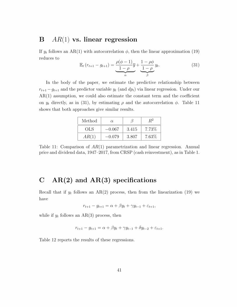
B AR(1) vs. linear regression

If yt follows an AR(1) with autocorrelation φ, then the linear approximation (19)

reduces to

Et (rt+1 − gt+1) =ρ(φ− 1)

1− ρy︸ ︷︷ ︸

α

+1− ρφ1− ρ︸ ︷︷ ︸β

yt. (31)

In the body of the paper, we estimate the predictive relationship between

rt+1−gt+1 and the predictor variable yt (and dpt) via linear regression. Under our

AR(1) assumption, we could also estimate the constant term and the coefficient

on yt directly, as in (31), by estimating ρ and the autocorrelation φ. Table 11

shows that both approaches give similar results.

Method α β R2

OLS −0.067 3.415 7.73%

AR(1) −0.079 3.807 7.63%

Table 11: Comparison of AR(1) parametrization and linear regression. Annualprice and dividend data, 1947–2017, from CRSP (cash reinvestment), as in Table 1.

C AR(2) and AR(3) specifications

Recall that if yt follows an AR(2) process, then from the linearization (19) we

have

rt+1 − gt+1 = α + βyt + γyt−1 + εt+1,

while if yt follows an AR(3) process, then

rt+1 − gt+1 = α + βyt + γyt−1 + δyt−2 + εt+1.

Table 12 reports the results of these regressions.

41

2 4 6 8 10 12

0.2

0.4

0.6

0.8

1.0

Figure 8: Partial autocorrelations of yt. Annual data, 1947–2017, cash-reinvestment method.

a s.e. β s.e. γ s.e. δ s.e. R2

AR(1) −0.067 [0.049] 3.415 [1.317] 7.73%

AR(2) −0.056 [0.053] 6.098 [3.378] −2.991 [3.339] 8.84%

AR(3) −0.040 [0.055] 6.473 [3.313] 0.651 [3.231] −4.457 [2.373] 11.32%

Table 12: Predictive regressions for S&P 500, annual data, cash reinvestment,1947–2017.

D Nonlinear specifications

In this section we consider the effect of allowing for quadratic or cubic functional

relationships between rt+1 − gt+1 and yt. We run the regressions

rt+1 − gt+1 = a0 + a1yt + a2y2t + εt+1

and

rt+1 − gt+1 = a0 + a1yt + a2y2t + a3y

3t + εt+1.

E Bt vs. other financial indicators

42

a0 s.e. a1 s.e. a2 s.e. a3 s.e. R2

linear −0.067 [0.049] 3.415 [1.317] 7.73%

quadratic −0.072 [0.111] 3.740 [6.348] −4.390 [81.25] 7.73%

cubic −0.12 [0.23] 9.35 [20.96] −166.4 [576.0] 1402.8 [4821.3] 7.81%

Table 13: Predictive regressions for S&P 500, annual data, cash reinvestment,1947–2017.

0.01 0.02 0.03 0.04 0.05 0.06 0.07yt

-0.2

-0.1

0.1

0.2

0.3

0.4

Et(rt+1-gt+1)

01/96

12/99

12/17

(a) Cubic.

0.01 0.02 0.03 0.04 0.05 0.06 0.07yt

-0.2

-0.1

0.1

0.2

0.3

0.4

Et(rt+1-gt+1)

01/96

12/99 12/17

(b) Linear.

Figure 9: Forecasting with cubic and linear specifications at the beginning (01/96)and end (12/17) of our sample, and around the market highs in 12/99. Linesindicate the estimated functional relationship between Et (rt+1 − gt+1) and yt, anddots indicate the specific values of yt and Et (rt+1 − gt+1) that happened to prevailon the relevant dates.

corr(Bt, ·) Level p-value

ER1yr 0.381 0.000

ER10yr 0.695 0.000

DM survey 0.286 0.000

EER1yr −0.567 0.000

ERstd1yr −0.224 0.003

EER10yr −0.278 0.021

ERstd10yr −0.270 0.005

Table 14: Correlation coefficients, computed using quarterly data between2000:Q2 and 2017:Q4 (Graham–Harvey series) or between 2003:Q1 and 2015:Q3(De la O–Myers series), with bootstrapped p-values.

43

Bt

vt

2000 2005 2010 2015

-2

-1

0

1

2

(a) Sentiment indicator and detrended vol-ume.

-30 -20 -10 0 10 20 30k

0.2

0.3

0.4

0.5

0.6

0.7

0.8

0.9

corr(Bt+k,vt)

(b) Correlation between Bt+k and de-trended volume at time t.

Figure 10: Sentiment indicator vs. detrended log volume (using the full sampleto construct each series). The shaded area in the right-hand panel indicates thebootstrapped 95% confidence interval.

44

Bt

EBPt

2000 2005 2010 2015

-1

0

1

2

3

4

5

6

(a) Bt and EBP.

-30 -20 -10 10 20 30k

-0.4

-0.2

0.2

0.4

0.6corr(Bt+k, EBPt)

(b) corr(Bt+k,EBPt).

Bt

NFCIt

2000 2005 2010 2015

-1

0

1

2

3

4

5

6

(c) Bt and NFCI.

-30 -20 -10 10 20 30k

-0.4

-0.2

0.2

0.4

corr(Bt+k, NFCIt)

(d) corr(Bt+k,NFCIt).

Bt

ANFCIt

2000 2005 2010 2015

-1

0

1

2

3

4

5

6

(e) Bt and ANFCI.

-30 -20 -10 10 20 30k

-0.1

0.1

0.2

0.3

0.4

0.5corr(Bt+k, ANFCIt)

(f) corr(Bt+k,ANFCIt).

Figure 11: The relationship between Bt and various measures of financial con-ditions. Shaded areas in the right panels indicate bootstrapped 95% confidenceintervals.

45

2000 2005 2010 20150.02

0.04

0.06

0.08

0.10

0.12

ER 1 year Bt

(a) Bt vs. ER1yr (Graham–Harvey)

2000 2005 2010 2015

0.02

0.04

0.06

0.08

0.10

0.12

ER 10 years Bt

(b) Bt vs. ER10yr (Graham–Harvey)

2000 2005 2010 2015

-0.1

0.0

0.1

0.2

0.3

Survey Et[gt+1] Bt

(c) Bt vs. survey based expected dividend growth (De la O–Myers)

Figure 12: Bt plotted against other sentiment measures (I).

46

2000 2005 2010 2015

0.02

0.04

0.06

0.08

0.10

0.12

EER 1 year Bt

(a) Bt vs. EER1yr (Graham–Harvey)

2000 2005 2010 20150.02

0.04

0.06

0.08

0.10

0.12

Disagreement 1 year Bt

(b) Bt vs. EERstd1yr (Graham–Harvey)

2000 2005 2010 2015

0.02

0.04

0.06

0.08

0.10

0.12

EER 10 years Bt

(c) Bt vs. EER10yr (Graham–Harvey)

2000 2005 2010 2015

0.02

0.04

0.06

0.08

0.10

0.12

Disagreement 10 years Bt

(d) Bt vs. EERstd10yr (Graham–Harvey)

Figure 13: Bt plotted against other sentiment measures (II).

47