volatility forecasting by quantile regression

This article was downloaded by: [University of Connecticut]On: 08 October 2014, At: 12:37Publisher: RoutledgeInforma Ltd Registered in England and Wales Registered Number: 1072954 Registered office: Mortimer House,37-41 Mortimer Street, London W1T 3JH, UK

Applied EconomicsPublication details, including instructions for authors and subscription information:http://www.tandfonline.com/loi/raec20

Volatility forecasting by quantile regressionAlex YiHou Huang aa Department of Finance , Yuan Ze University , 135 Yuan-Tung Road, Chung-Li 320, Taoyuan,Taiwan, ROCPublished online: 02 Feb 2011.

To cite this article: Alex YiHou Huang (2012) Volatility forecasting by quantile regression, Applied Economics, 44:4, 423-433,DOI: 10.1080/00036846.2010.508727

To link to this article: http://dx.doi.org/10.1080/00036846.2010.508727

PLEASE SCROLL DOWN FOR ARTICLE

Taylor & Francis makes every effort to ensure the accuracy of all the information (the “Content”) containedin the publications on our platform. However, Taylor & Francis, our agents, and our licensors make norepresentations or warranties whatsoever as to the accuracy, completeness, or suitability for any purpose of theContent. Any opinions and views expressed in this publication are the opinions and views of the authors, andare not the views of or endorsed by Taylor & Francis. The accuracy of the Content should not be relied upon andshould be independently verified with primary sources of information. Taylor and Francis shall not be liable forany losses, actions, claims, proceedings, demands, costs, expenses, damages, and other liabilities whatsoeveror howsoever caused arising directly or indirectly in connection with, in relation to or arising out of the use ofthe Content.

This article may be used for research, teaching, and private study purposes. Any substantial or systematicreproduction, redistribution, reselling, loan, sub-licensing, systematic supply, or distribution in anyform to anyone is expressly forbidden. Terms & Conditions of access and use can be found at http://www.tandfonline.com/page/terms-and-conditions

http://www.tandfonline.com/loi/raec20

http://www.tandfonline.com/action/showCitFormats?doi=10.1080/00036846.2010.508727

http://dx.doi.org/10.1080/00036846.2010.508727

http://www.tandfonline.com/page/terms-and-conditions

http://www.tandfonline.com/page/terms-and-conditions

Applied Economics, 2012, 44, 423–433

Volatility forecasting by quantile

regression

Alex YiHou Huang

Department of Finance, Yuan Ze University, 135 Yuan-Tung Road,

Chung-Li 320, Taoyuan, Taiwan, ROC

E-mail: [email protected]

Quantile regression allows one to predict the volatility of time series

without assuming an explicit form for the underlying distribution.

Financial assets are known to have irregular return patterns; not only

the volatility but also the distribution functions themselves may vary with

time, so traditional time series models are often unreliable. This study

presents a new approach to volatility forecasting by quantile regression

utilizing a uniformly spaced series of estimated quantiles. The proposed

method provides much more complete information on the underlying

distribution, without recourse to an assumed functional form. Based on an

empirical study of seven stock indices, using 16 years of daily return data,

the proposed approach produces better volatility forecasts for six of the

seven indices.

I. Introduction

Volatility forecasting has been a key research subject

in financial economics for the past two decades.

Volatility can be interpreted as the level of uncer-

tainty in a financial asset, and is applicable to many

risk management processes. It is also a critical input

variable in pricing financial derivatives, and thus

plays a central role in investment decisions (Maris

et al., 2007). Despite its importance, however,

researchers and practitioners have still not gained a

full understanding of volatility behaviours, and the

mystery of the volatility smile is one striking example.The volatility of financial markets has also become

an important economic indicator. Events with a

negative impact on financial markets, for example,

the 9/11 attacks and the recent subprime mortgage

market crash, may be quantified and analysed

through their effect on volatility. As public confi-

dence and economic conditions are highly correlated

with the current financial market uncertainty, many

governments lean heavily on volatility forecasts when

making key policy decisions. Accurate volatility

forecasts of financial assets and markets are, there-

fore, in high demand, and academic researchers have

devoted tremendous resources to producing better

forecasts.In this article, a new model is presented for

generating volatility forecasts by quantile regression.

As literature has established, the specific return

distributions assumed by the popular Generalized

Autoregressive Conditional Heteroscedasticity

(GARCH) models are often inconsistent with the

practical behaviour of financial assets. Two alterna-

tive approaches, Stochastic Volatility (SV) modelling

and options-based volatility forecasting, require

restricted model specifications and derivative data

series, respectively: information that is simply una-

vailable for some financial assets. On the other hand,

it is possible to estimate quantiles directly from

product data without the need for complex modelling

or specific assumptions concerning the underlying

distribution. One can therefore apply quantiles

directly to volatility forecasting, as long as a signif-

icant relationship between quantiles and volatility can

be established. Our proposed model demonstrates the

Applied Economics ISSN 0003–6846 print/ISSN 1466–4283 online � 2012 Taylor & Francis 423http://www.informaworld.com

DOI: 10.1080/00036846.2010.508727

Dow

nloa

ded

by [

Uni

vers

ity o

f C

onne

ctic

ut]

at 1

2:37

08

Oct

ober

201

4

connection between these two variables with signif-icant empirical results.

The next section will conduct a brief review of theexisting volatility models. This article will thenpresent the new methodology and discuss theempirical findings.

II. Literature Review

By definition, the volatility of a financial asset is theSD, �, of its return distribution. Given a sample of mreturns, its best estimate � is given by the followingequations:

�2 ¼1

m� 1

Xmt¼1

rt � �rð Þ2, where

rt ¼ lnSt

St�1

� �ð1Þ

here rt is the continuously compounded return of theasset during day t, �r the mean of all m returns in thesample and St the market value of the asset on day t.

The SD of past returns is a natural predictor of �.There are a number of models that estimate volatilitybased on its past values, and the simplest model is thehistorical average, which uses Equation 1 to calculate�t�1 and assumes that it is equal to �t. The key issuewith this method is its dependence on the samplesize m. When m is too small, the method might have alarge sampling error. If m is too large, however, moreremote data may not accurately reflect the currentmarket conditions.

In order to increase m while still placing enoughemphasis on the latest market conditions, the movingaverage and Exponentially Weighted MovingAverage (EWMA) models assign larger weights tomore recent data. Another popular time series modelin volatility forecasting is the GARCH methodpioneered by Bollerslev (1986) and Taylor (1986).The model treats volatility as a time-varying andtime-dependent component with the following func-tional form:

�2t ¼ �1 þ �2�2t�1 þ �3"

2t�1 ð2Þ

where "t�1 is the lagged error term and �’s theparameters for estimation. Various modifications tothe GARCH model have been proposed with focuson incorporating the attributes of specific financialassets, such as Exponential GARCH (EGARCH;Nelson, 1991), Regime-Switching GARCH

(RS-GARCH; Gray, 1996) and FractionallyIntegrated GARCH (FIGARCH; Baillie et al., 1996).

However, it is important to note that the actualvolatility � is not necessarily associated with anystandard distribution function. In fact, many priorresearches have found that the return distributions offinancial assets are rarely Gaussian (Hull and White,1998) and may follow common examples includingstudent’s t-distribution, the stable Paretian distribu-tion (Fabozzi et al., 2006), a mixture of normaldistributions (Venkataraman, 1997) and the general-ized error distribution (Nelson, 1991). Manyresearchers have also found that return distributionsare asymmetric, fat-tailed and nonconstant (Glostenet al., 1993; Neftci, 2000; Noh and Kim, 2006).Therefore, estimating � based on a constant assumeddistribution of returns can easily lead one tomisconstrue the real level of uncertainty.

Another development of ARCH in volatility fore-casting is the Switching ARCH (SWARCH) model-ling. The model was pioneered by Cai (1994) andHamilton and Susmel (1994) and later developed byFornari and Mele (1997). The key idea is wherevolatility follows different ARCH specifications indifferent states; therefore, conditional distributionsvary according to structural changes in variables. Onecommon specification of SWARCH for a returnvariable, yt, with error term, et, can be summarized asfollowing settings:

et ¼ffiffiffiffiffigstp

ut, ut ¼ffiffiffiffiht

pvt

where vt � Gaussian distribution

ht ¼ a0 þ a1u2t�1 þ a2u

2t�2 þ � � � þ aqu

2t�q

ð3Þ

here, st is an unobservable state variable which servesas the dynamics of changes between regimes, and itcan be structured according to return behaviours orassumed to follow the first-order Markov chainprocess. Previous studies have found thatSWARCH provides better model specifications offinancial assets and more accurate forecasting abilitythan other ARCH–GARCH models (Klaassen, 2002;Chiou et al., 2007; Li, 2007).

In addition to GARCH class, by modelling vola-tility as a stochastic variable, the SV modelling is ableto study the structure of volatility behaviour: itsdriving mechanisms, jumping patterns and character-istics of formation.1 In recent years, SV modelling hasgone through several significant refinements such asapplications of the Levy process.2 The main draw-back of the SV approach is the difficulty in applyingit to empirical data. Many SV models have no

1A detailed survey can be found in Ghysels et al. (1996).2 Please see Carr et al. (2003) and Wu (2008).

424 A. Y. Huang

Dow

nloa

ded

by [

Uni

vers

ity o

f C

onne

ctic

ut]

at 1

2:37

08

Oct

ober

201

4

closed-form solution, relying on complicated calibra-

tion procedures or statistical techniques to provide

estimates. This shortcoming has made the approach

less popular than GARCH models in the financial

industry.The last approach would be options-based volatil-

ity forecasting. Its main idea is to use the prices of

financial assets and their respective options, along

with some specific option pricing models, to generate

the volatility forecast implied by the arbitrage-free

condition.3 This approach has two main shortcom-

ings; first, multiple forecasts can be derived for

a single financial asset by choosing a different

series of options. Second, an option series must be

available to use the method, and there are many

financial assets with economically important volatil-

ity forecasts; however, they do not have option

derivatives.Taylor (2005) utilizes Value at Risk (VaR) esti-

mates from quantile regression for volatility forecast-

ing. Specifically, he applies the Conditional Value at

Risk by Quantile Regression (CAViaR) models

proposed by Engle and Manganelli (2004) to produce

VaR estimates at the needed probability levels. He

then produces volatility forecasts using the interval

approximation approach presented in Pearson and

Tukey (1965). This study proposed the following

simple approximations to the SD based on symmetric

quantiles of the sample:

� ¼Qð0:99Þ � Qð0:01Þ

4:65, � ¼

Qð0:975Þ � Qð0:025Þ

3:92,

� ¼Qð0:95Þ � Qð0:05Þ

3:25ð4Þ

where Qð1� �Þ and Qð�Þ are the estimated quantiles

for a cumulative probability �. The denominators of

Equation 4 are based on the central distances between

the desired quantiles under Pearson curves4 and are

slightly different from the denominators of 4.653

(¼2.326� 2), 3.92 (¼1.96� 2) and 3.29 (¼1.645� 2),

respectively, under Gaussian distribution. Taylor

(2005) extended this idea by proposing a quadratic

regression model as follows:

�2tþ1 ¼ �1 þ �1 Qtþ1ð1� �Þ � Qtþ1ð�Þ� �2

ð5Þ

where �2tþ1 is the volatility forecast at time tþ 1 for

a series extending to time t and �1 and �1 the

parameters to be estimated from the sample. The

author concluded that the regression approach to

volatility forecasting outperformed GARCH models

and moving average method by examining forecast-ing performances of 25 stock indices and individualstocks.

III. Volatility Forecasting by QuantileRegression

A new approach for volatility forecasting by quantileregression is proposed. The method requires one togenerate estimates of the return distribution quantileswithout any specific assumptions concerning thedistribution function itself. The estimated quantilescan, therefore, be applied directly to volatility fore-casts, either by approximating the relationshipbetween quantiles and the variance, or by certainregression models. This research extends the study ofTaylor (2005), summarized in the previous section,presenting an alternative model for this relationshipand a more general approach.

Engle and Manganelli (2004) presented four dif-ferent autoregressive models for generating the con-ditional quantiles for VaR estimates:

Adaptive: Qtð�Þ ¼Qt�1ð�Þ

þ�ð½1þexpðG½rt�1

�Qt�1ð�Þ�Þ��1� �Þ

Symmetric absolute;value: Qtð�Þ ¼�1þ�2Qt�1ð�Þ

þ�3 rt�1j j

Asymmetric slope: Qtð�Þ ¼�1þ�2Qt�1ð�Þ

þ�3maxðrt�1,0Þ

��4minðrt�1,0Þ

IndirectGARCHð1,1Þ: Qtð�Þ ¼��1þ�2Q

2t�1ð�Þ

þ�3r2t�1

�1=2In all these examples, G is a positive finite number,

rt the portfolio return and �’s the parameters to beestimated based on the following minimizationcondition:

min�

Xrt�Qtð�Þ

� rt �Qtð�Þ þ X

rt5Qtð�Þ

1� �ð Þ rt �Qtð�Þ ( )

ð6Þ

Thus, these models estimate VaR based on returnpatterns over a one lag period. Without any explicitdistributional assumptions, the conditional quantilesand forecasted VaR are generated by analysing theserial dependence of the quantiles on the returnbehaviours according to the latest market conditions.Taylor (2005) used Equations 4 and 5 to incorporate

3A detailed survey is given in Poon and Granger (2003).4A detailed survey can be found in Pearson and Tukey (1965).

Volatility forecasting by quantile regression 425

Dow

nloa

ded

by [

Uni

vers

ity o

f C

onne

ctic

ut]

at 1

2:37

08

Oct

ober

201

4

the estimated VaR into the volatility forecast by using

98%, 95% and 90% quantile intervals.5 To elaborate,

the distance between the symmetric quantiles of a

distribution can be used as the key explanatory

variable to explain second moment behaviours

such as volatility. While this method has

been found to produce robust empirical results, it is

natural to ask whether the choice of any single

quantile pair can be justified and/or optimized.

For example, one might wonder if just one pair of

quantiles is enough to accurately explain the volatility

behaviour. In this article, several alternative versions

of Taylor’s model are provided in order to address

this issue.Instead of using one pair of quantiles, this study

uses a uniformly spaced series of quantiles. The

movements of these quantiles not only reflect the tail

behaviours, but also the whole distributional pattern.

In this manner, one can incorporate the distributional

behaviours into volatility forecasting and avoid

overestimation from extremely asymmetric tails or

underestimation from highly symmetric tails.

Specifically, the following model is employed:

�tþ1 ¼ �1 þ �1F Qtþ1ð�Þ� �

ð7Þ

where F(�) represents an unspecified function and

Qtþ1ð�Þ a vector of quantiles {�, 2�, . . . ,m�} to be

estimated at time t þ1 (�40, m�51). Ideally, one

should use as many quantiles as possible to fully

explain the behaviour of the distribution. In this

study, � is set to be 0.01, covering the percentiles

{1, 2, . . . , 99}. This article also considers three differ-

ent functions of F(�), which are shown in the

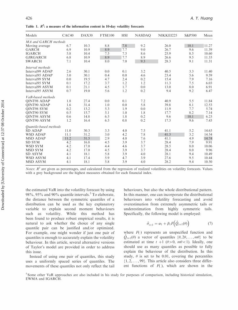
Table 1. R2: a measure of the information content in 10-day volatility forecasts

Models CAC40 DAX30 FTSE100 HSI NASDAQ NIKKEI225 S&P500 Mean

MA and GARCH methodsMoving average 6.7 10.3 8.8 7.8 9.2 26.0 10.1 11.27GARCH 6.9 10.9 8.9 7.7 9.0 26.7 9.6 11.39IGARCH 5.8 10.4 7.5 7.5 8.6 25.9 8.5 10.60GJRGARCH 6.8 10.9 8.9 7.7 8.9 26.6 9.5 11.33SWARCH 7.1 10.4 8.0 7.0 9.3 28.3 9.1 11.31

Interval methodsInterval99 ADAP 2.6 30.1 0.0 0.1 3.2 40.5 3.3 11.40Interval95 ADAP 3.0 30.1 0.4 0.0 4.6 23.4 5.6 9.59Interval99 SYM 0.0 19.5 4.7 2.4 0.2 15.4 7.9 7.16Interval95 SYM 0.1 17.2 3.7 1.2 1.2 11.3 7.5 6.03Interval99 ASYM 0.1 21.1 4.5 1.7 0.0 13.0 8.0 6.91Interval95 ASYM 0.7 19.0 5.6 1.2 0.2 9.4 9.2 6.47

VaR-based methodsQINT98 ADAP 1.8 27.4 0.0 0.1 7.2 40.9 5.5 11.84QINT90 ADAP 1.6 31.4 1.0 0.0 5.8 39.8 8.1 12.53QINT98 SYM 0.2 13.2 5.3 1.9 0.0 11.9 7.7 5.74QINT90 SYM 0.5 15.7 5.1 1.0 1.8 17.7 8.2 7.14QINT98 ASYM 0.6 14.8 6.5 1.8 0.2 9.6 10.1 6.23QINT90 ASYM 1.2 16.4 6.5 0.8 0.2 17.3 9.6 7.43

Quantile-based methodsSD ADAP 11.0 30.3 3.3 4.0 7.5 41.1 5.2 14.63WSD ADAP 11.1 31.2 3.0 4.2 7.8 41.3 3.2 14.54MSD ADAP 11.2 31.5 2.9 4.0 7.6 41.1 4.9 14.74SD SYM 4.2 16.8 4.5 3.9 3.7 28.4 7.9 9.91WSD SYM 4.2 17.0 4.4 4.6 3.7 28.5 8.0 10.06MSD SYM 4.2 17.0 4.5 3.9 3.7 28.4 8.0 9.96SD ASYM 4.1 18.1 5.8 3.9 4.0 28.1 9.4 10.49WSD ASYM 4.1 17.4 5.9 4.7 3.9 27.6 9.5 10.44MSD ASYM 4.1 18.1 5.8 3.9 4.0 28.2 9.4 10.50

Notes: R2 are given as percentages, and calculated from the regression of realized volatilities on volatility forecasts. Valueswith a grey background are the highest measures obtained for each financial index.

5 Some other VaR approaches are also included in his study for purposes of comparison, including historical simulation,EWMA and IGARCH.

426 A. Y. Huang

Dow

nloa

ded

by [

Uni

vers

ity o

f C

onne

ctic

ut]

at 1

2:37

08

Oct

ober

201

4

following equations. In each case, �Q is the conditional

mean of all quantiles.

SD: Fð�Þ ¼1

m�1

X99m¼1

Qð0:01mÞ� �Q� �2 !1=2

Weighted SD: Fð�Þ ¼X99m¼1

W Qð0:01mÞ� �Q� �2 !1=2

Median SD: Fð�Þ ¼1

m�2

X99m¼1

Qð0:01mÞ�Qð0:5Þð Þ2

!1=2

Thus, instead of a single symmetric pair, this

approach incorporates all the estimated quantiles into

the volatility forecast. All the SD functions given

above represent the width of the distribution of the

estimated quantiles around their conditional mean,

albeit in slightly different ways. The second SD

function applies a weight W to each squared devia-

tion in the sum. W is set as �/25 when �� 0.5, and

(1��)/25 otherwise. This ensures that extreme

quantiles will have a greater impact on the volatilityforecasts and designs to incorporate the often foundleptokurtosis return distributions of financial assets.The third SD function recognizes that many returndistributions are somewhat irregular; the median ismore representative of their centre than the mean.

IV. Empirical Findings

The empirical study uses more than 16 years(1 January 1990 to 25 July 2007) of daily returnsfrom seven major stock indices: France’s CAC40,Germany’s DAX30, the UK’s FTSE100, HongKong’s HSI, Japan’s Nikkei225 and the US’sNASDAQ and S&P500. All data are taken from theDataStream database. The earliest 3500 data pointsare used for model estimation: the first 3000 forquantile estimation and the next 500 for volatilityforecasting. Depending on the number of holidays,

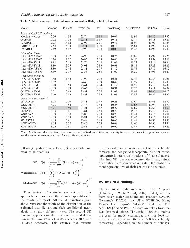
Table 2. MSE: a measure of the information content in 10-day volatility forecasts






Notes: MSEs are calculated from the regression of realized volatilities on volatility forecasts. Values with a grey backgroundare the lowest measures obtained for each financial index.


Dow

nloa

ded

by [

Uni

vers

ity o

f C

onne

ctic

ut]

at 1

2:37

08

Oct

ober

201

4

this leaves from 856 (Nikkei225) to 957 (NASDAQ)

out-of-sample data for evaluating the forecasts.Volatility forecasts are compared from the follow-

ing models:

(1) Moving average: the historical average method

described in Section II and Equation 1.

A simple 30-day average is used in this model.(2) GARCH: The GARCH(1,1) method, as

described in Section II.(3) IGARCH: integrated GARCH as proposed by

Nelson (1990), where the coefficients in

Equation 2 integrate to one.(4) GJRGARCH: in this model, proposed

by Glosten et al. (1993), an indicator function

is imposed on the coefficient of lag return.

The functional form is

�2t ¼ �1 þ �2�2t�1 þ ð1� I½"t�1 4 0�Þ�3"

2t�1

þ ðI½"t�1 4 0�Þ�4"2t�1

(5) SWARCH: the switching ARCH model shown

in Equation 3 with state variable following theMarkov chain process.

(6) Interval models: the approach of approximat-

ing second moments from quantiles originally

proposed by Pearson and Tukey (1965).

As described in Equation 4, they proposed

three different quantile pairs, and four regres-

sion functions described in Section III are

considered. Based on previous applications andreviews of this methodology (Taylor, 2005;

Kuester et al., 2006), we have selected two

intervals, 99 and 95, and three regression

functions: Adaptive (ADAP), Symmetric

(SYM) and Asymmetric (ASYM). Therefore,

a total of six models are applied in this

category: Interval99 ADAP, Interval95

ADAP, Interval99 SYM, Interval95 SYM,

Interval99 ASYM and Interval95 ASYM.(7) VaR-based models: the method proposed by

Taylor (2005), described in Section III as

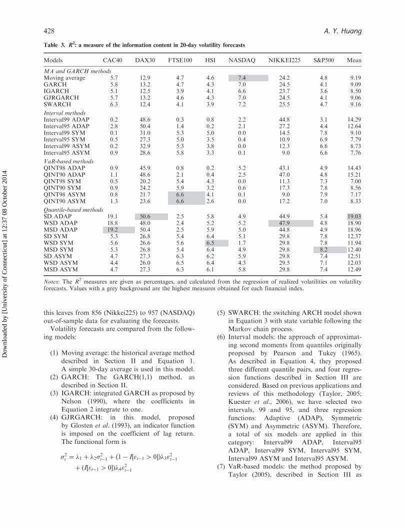
Table 3. R2: a measure of the information content in 20-day volatility forecasts






Notes: The R2 measures are given as percentages, and calculated from the regression of realized volatilities on volatilityforecasts. Values with a grey background are the highest measures obtained for each financial index.

428 A. Y. Huang

Dow

nloa

ded

by [

Uni

vers

ity o

f C

onne

ctic

ut]

at 1

2:37

08

Oct

ober

201

4

Equation 7. Taylor examined three differentintervals as the explanatory variable, findingthat quantile separations of 98% and 90%perform better than a separation of 95%. Bothquantile pairs (98 and 90) are thus used to thethree regression functions mentioned in case 5,composing the following six models: QINT98ADAP, QINT90 ADAP, QINT98 SYM,QINT90 SYM, QINT98 ASYM and QINT90ASYM.

(8) Quantile regression models: method proposedby this study as described in Section III. Thereare three quantile regression functions selectedand three ways to combine the series ofquantiles into an explanatory variable: SD,Weighted SD (WSD) and Median SD (MSD).Therefore, the following nine models are con-sidered in the empirical application: (1) SDADAP, (2) WSD ADAP, (3) MSD ADAP,(4) SD SYM, (5) WSD SYM, (6) MSD SYM,(7) SD ASYM, (8) WSD ASYM and (9) MSDASYM.

In total, there are 26 models to apply to the sevenstock indices. Realized volatilities from the out-of-sample comparison over 10- and 20-day periods areregressed onto each of the model volatility forecasts.Following Taylor (2005), the R2 coefficients of theseordinary least squares regressions are reported to seehow much of the realized volatility is explained by theforecasts. In addition, Mean Squared Errors (MSEs)from the regressions are also presented to determinethe goodness-of-fit. Tables 1 and 2 summarize theoutcomes of 10-day periods for R2 coefficients andMSE, respectively.

Table 1 presents the ability of various volatilitymodels to explain the 10-day volatilities realized inthe out-of-sample data, expressed as a percentage; thehigher the coefficient, the better the predictive powerof the model. For the CAC40 index, MSD ADAP hasthe highest measure as 11.2. In fact, all three quantileregression models using the adaptive regressionfunction produce similar results. Measures from allother models are significantly lower. For the DAX30index, the same model (MSD ADAP) performs best

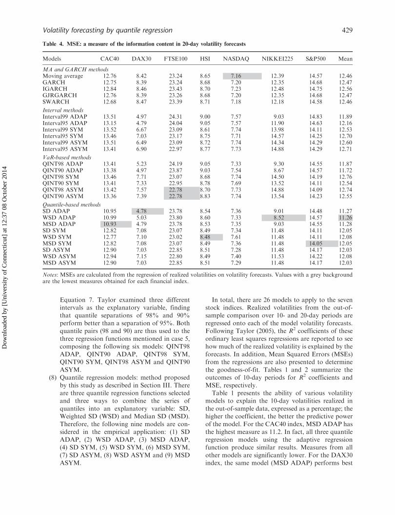
Table 4. MSE: a measure of the information content in 20-day volatility forecasts






Notes: MSEs are calculated from the regression of realized volatilities on volatility forecasts. Values with a grey backgroundare the lowest measures obtained for each financial index.


Dow

nloa

ded

by [

Uni

vers

ity o

f C

onne

ctic

ut]

at 1

2:37

08

Oct

ober

201

4

with a measure of 31.5. For the FTSE100 index, it isGARCH and GJRGARCH that have the highestmeasures of 8.9.

For the HSI and NASDAQ indices, the movingaverage method and SWARCH performs best withmeasures of 7.8 and 9.3, respectively. For theNikkei225 index, quantile regression model WSDADAP outperforms all others, with an R2 of 41.3.Finally, for the S&P500 index, moving averages andthe QINT98 ASYM interval model produce thehighest measure of 10.1. GARCH and asymmetricquantile regression also have reasonably high mea-sures, in the range 9.4–9.6. If we consider the averageover all the seven indices, we find that quantileregression models with adaptive regression score thehighest, with measures between 14.54 and 14.74. TheVaR-based adaptive interval models have the nextbest measures, with values ranging from 11.84to 12.53.

To summarize Table 1, quantile models with anadaptive regression function and the moving averagemodel each achieve the best R2 measure for three andtwo indices, respectively. In terms of the average over

all indices, however, quantile regression modelsachieve scores about 30% higher than the movingaverage method. In addition, within the quantileframework, models with an adaptive regressionfunction perform better than those with symmetricor asymmetric functions, and the finding is consistentwith prior research (Kuester et al., 2006).

Table 2 presents the MSE measures as alternativeindicator of model fit. The comparisons of perfor-mances between the models for each index are thesame as Table 1, since the sample period and totalsum of squares of realized volatility in each index areidentical among models. However, the measuresreveal forecasting performances between the indicesto be different from R2 coefficients. For instance, theUK FTSE100 has the highest MSE in average butbetter R2 coefficients in average than CAC40 andHSI. This result is due to relatively higher variationsof the realized volatility of FTSE100 than the othertwo indices. An opposite observation can be foundedfor Nikkei225 with best average R2 coefficients givenin Table 1, but has a relatively lower average MSEthan CAC40 and FTSE100.

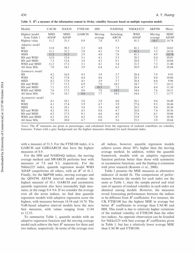
Table 5. R2: a measure of the information content in 10-day volatility forecasts based on multiple regression models


Highest modelfrom Table 1

MSDADAP

MSDADAP

GARCH Movingaverage

SwitchingARCH

WSDADAP

Movingaverage

MSDADAP

Highest value 11.2 31.5 8.9 7.8 9.3 41.3 10.1 14.74

Adaptive modelSD 11.0 30.3 3.3 4.0 7.5 41.1 5.2 14.63WSD 11.1 31.2 3.0 4.2 7.8 41.3 3.2 14.54MSD 11.2 31.5 2.9 4.0 7.6 41.1 4.9 14.74SD and WSD 11.0 15.6 3.1 4.1 5.3 28.2 8.4 10.81SD and MSD 7.3 15.8 3.8 4.2 9.1 28.0 7.7 10.84WSD and MSD 11.2 17.2 3.1 4.1 5.4 31.5 7.3 11.40All three SDs 7.0 14.1 3.9 6.8 6.3 28.9 8.9 10.84

Symmetric modelSD 4.2 16.8 4.5 3.9 3.7 28.4 7.9 9.91WSD 4.2 17.0 4.4 4.6 3.7 28.5 8.0 10.06MSD 4.2 17.0 4.5 3.9 3.7 28.4 8.0 9.96SD and WSD 7.7 17.5 8.9 7.8 14.5 34.7 7.7 14.11SD and MSD 7.1 15.3 4.7 10.3 7.3 26.4 6.6 11.10WSD and MSD 7.6 17.5 9.0 7.8 14.7 34.6 7.6 14.11All three SDs 7.8 14.7 9.6 7.7 14.5 34.4 7.7 13.77

Asymmetric modelSD 4.1 18.1 5.8 3.9 4.0 28.1 9.4 10.49WSD 4.1 17.4 5.9 4.7 3.9 27.6 9.5 10.44MSD 4.1 18.1 5.8 3.9 4.0 28.2 9.4 10.50SD and WSD 4.2 19.1 4.5 8.0 4.7 26.0 7.4 10.56SD and MSD 4.5 17.5 8.1 4.6 4.0 27.6 4.1 10.06WSD and MSD 4.2 19.2 4.5 8.0 4.7 25.9 7.0 10.50All three SDs 5.0 20.0 6.7 8.0 5.6 25.3 3.9 10.64


430 A. Y. Huang

Dow

nloa

ded

by [

Uni

vers

ity o

f C

onne

ctic

ut]

at 1

2:37

08

Oct

ober

201

4

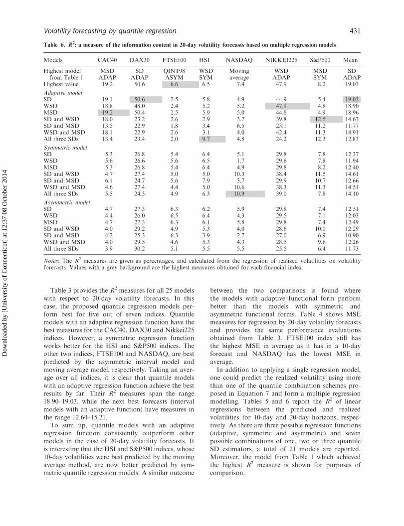
Table 3 provides the R2 measures for all 25 modelswith respect to 20-day volatility forecasts. In thiscase, the proposed quantile regression models per-form best for five out of seven indices. Quantilemodels with an adaptive regression function have thebest measures for the CAC40, DAX30 and Nikkei225indices. However, a symmetric regression functionworks better for the HSI and S&P500 indices. Theother two indices, FTSE100 and NASDAQ, are bestpredicted by the asymmetric interval model andmoving average model, respectively. Taking an aver-age over all indices, it is clear that quantile modelswith an adaptive regression function achieve the bestresults by far. Their R2 measures span the range18.90–19.03, while the next best forecasts (intervalmodels with an adaptive function) have measures inthe range 12.64–15.21.

To sum up, quantile models with an adaptiveregression function consistently outperform othermodels in the case of 20-day volatility forecasts. Itis interesting that the HSI and S&P500 indices, whose10-day volatilities were best predicted by the movingaverage method, are now better predicted by sym-metric quantile regression models. A similar outcome

between the two comparisons is found wherethe models with adaptive functional form performbetter than the models with symmetric andasymmetric functional forms. Table 4 shows MSEmeasures for regression by 20-day volatility forecastsand provides the same performance evaluationsobtained from Table 3. FTSE100 index still hasthe highest MSE in average as it has in a 10-dayforecast and NASDAQ has the lowest MSE inaverage.

In addition to applying a single regression model,one could predict the realized volatility using morethan one of the quantile combination schemes pro-posed in Equation 7 and form a multiple regressionmodelling. Tables 5 and 6 report the R2 of linearregressions between the predicted and realizedvolatilities for 10-day and 20-day horizons, respec-tively. As there are three possible regression functions(adaptive, symmetric and asymmetric) and sevenpossible combinations of one, two or three quantileSD estimators, a total of 21 models are reported.Moreover, the model from Table 1 which achievedthe highest R2 measure is shown for purposes ofcomparison.

Table 6. R2: a measure of the information content in 20-day volatility forecasts based on multiple regression models


Highest modelfrom Table 1

MSDADAP

SDADAP

QINT98ASYM

WSDSYM

Movingaverage

WSDADAP

MSDSYM

SDADAP

Highest value 19.2 50.6 6.6 6.5 7.4 47.9 8.2 19.03

Adaptive modelSD 19.1 50.6 2.5 5.8 4.9 44.9 5.4 19.03WSD 18.8 48.0 2.4 5.2 5.2 47.9 4.8 18.90MSD 19.2 50.4 2.5 5.9 5.0 44.8 4.9 18.96SD and WSD 18.0 23.2 2.6 2.9 3.7 39.8 12.5 14.67SD and MSD 13.5 22.9 1.8 3.4 6.5 23.1 11.2 11.77WSD and MSD 18.1 22.9 2.6 3.1 4.0 42.4 11.3 14.91All three SDs 13.4 23.4 2.0 9.7 4.8 24.2 12.3 12.83

Symmetric modelSD 5.3 26.8 5.4 6.4 5.1 29.8 7.8 12.37WSD 5.6 26.6 5.6 6.5 1.7 29.8 7.8 11.94MSD 5.3 26.8 5.4 6.4 4.9 29.8 8.2 12.40SD and WSD 4.7 27.4 5.0 5.0 10.3 38.4 11.5 14.61SD and MSD 6.1 24.7 5.6 7.9 3.7 29.9 10.7 12.66WSD and MSD 4.6 27.4 4.4 5.0 10.6 38.3 11.3 14.51All three SDs 5.5 24.3 4.9 6.3 10.9 39.0 7.8 14.10

Asymmetric modelSD 4.7 27.3 6.3 6.2 5.9 29.8 7.4 12.51WSD 4.4 26.0 6.5 6.4 4.3 29.5 7.1 12.03MSD 4.7 27.3 6.3 6.1 5.8 29.8 7.4 12.49SD and WSD 4.0 29.2 4.9 5.3 4.0 28.6 10.0 12.29SD and MSD 4.2 25.3 6.3 3.9 2.7 27.0 6.9 10.90WSD and MSD 4.0 29.5 4.6 5.3 4.3 28.5 9.6 12.26All three SDs 3.9 30.2 5.1 5.5 5.5 25.5 6.4 11.73



Dow

nloa

ded

by [

Uni

vers

ity o

f C

onne

ctic

ut]

at 1

2:37

08

Oct

ober

201

4

Table 5 reports the outcome of this analysis for the10-day realized volatilities of all seven indices. We seethat the adaptive models still performs the best forthree indices. More importantly, indices FTSE100,HIS and NASDAQ, which were preferred by theGARCH, moving average or SWARCH models inTable 1, turn out to be better explained by symmetricquantile models. Only one index, the S&P500, is stillbest explained by a model other than the proposedquantile regression models.

Table 6 is analogous to Table 5 for 20-dayvolatilities. Here, six of the seven indices are nowbest predicted by quantile regression models. Thehighest mean measures in both Tables 5 and 6 areobtained by the same simple regression models foundin the previous comparisons: ADAP MSD for the10-day prediction and ADAP SD for the 20-dayprediction. Based on the comparison, we concludethat the proposed method outperforms the other timeseries models and previous quantile regression appli-cations in volatility forecasting.

V. Conclusions

Volatility is one indicator of the uncertainty in returnmovements for financial assets. It is also a key inputin derivative pricing, and an important variable inrisk management. Consequently, volatility forecast-ing has drawn a great deal of attention from bothacademic researchers and industrial practitioners.A wide variety of econometric models and mathe-matical methods have been developed to producebetter predictions of volatility.

In this article, a quantile regression approach tovolatility forecasting is presented. Quantileapproaches assume no explicit distribution, can beeasily applied and do not require a derivative dataseries. The proposed approach improves on previousquantile-based regressions by using an evenly spacedseries of estimated quantiles to construct the explan-atory variables. Not only does this remove thesomewhat arbitrary choice of which quantile pairbest represents the width of the distribution, but alsodoes provide much more complete information on thevolatility than was available to previous quantilemodels. For example, if the right and left tails of thereturn distribution, as well as all sections betweenthem, are driven by different forces, then thisapproach can perform better than other time seriesmodels.

An empirical study using the daily returns of sevenimportant financial indices shows that the proposedmodels nearly always outperform traditional methods.

For six of the seven stock indices, one or more versionsof the proposed approach generate better volatilityforecasts over both 10- and 20-day horizons.The adaptive functional form of quantile regressionperforms best in many cases.

The main shortcoming of the proposed approach isthat it requires significant computing resources.A long series of quantiles needs to be generated,and many different quantile regression functions needto be tested to determine the best specific model.Fortunately, improvements in technology have madethis drawback less critical. One possible extension tothis study would be to estimate higher moments ofthe return distribution from the quantile series,thereby gaining a deeper understanding of the vola-tility behaviour.

Acknowledgements

This research was partly supported by the NationalScience Council of Taiwan (NSC95-2415-H-155-004).The author thanks the referees for valuable commentsand Wen-Cheng Hu, Chin-Chun Chen and Sassa Linfor providing excellent research assistance.

References

Baillie, R. T., Bollerslev, T. and Mikkelsen, H. O. (1996)Fractionally integrated generalized autoregressiveconditional heteroscedasticity, Journal ofEconometrics, 74, 3–30.

Bollerslev, T. (1986) Generalized autoregressive conditionalheteroscedasticity, Journal of Econometrics, 31,307–28.

Cai, J. (1994) A Markov model of unconditional variancein ARCH, Journal of Business and Economic Statistics,12, 309–16.

Carr, P., Geman, H., Madan, D. B. and Yor, M. (2003)Stochastic volatility for Levy processes, MathematicalFinance, 13, 345–82.

Chiou, J., Wu, P., Chang, A. and Huang, B. (2007) Theasymmetric information and price manipulation instock market, Applied Economics, 39, 883–91.

Engle, R. F. and Manganelli, S. (2004) CAViaR: condi-tional autoregressive value at risk by regressionquantiles, Journal of Business and EconomicStatistics, 22, 367–81.

Fabozzi, F. J., Racheva-Iotova, B. and Stoyanov, V.(2006) An empirical examination of the returndistribution characteristics of agency mortgage pass-through securities, Applied Financial Economics, 16,1085–94.

Fornari, F. and Mele, A. (1997) Sign- and volatility-switching ARCH models: theory and applications tointernational stock markets, Journal of AppliedEconometrics, 12, 49–65.

432 A. Y. Huang

Dow

nloa

ded

by [

Uni

vers

ity o

f C

onne

ctic

ut]

at 1

2:37

08

Oct

ober

201

4

Ghysels, E., Harvey, A. and Renault, E. (1996) Stochasticvolatility, in Handbook of Statistics: StatisticalMethods in Finance, Vol. 14 (Eds) G. S. Maddalaand C. R. Rao, Elsevier Science, Amsterdam,pp. 119–91.

Glosten, L. R., Jagannathan, R. and Runkle, D. E. (1993)On the relation between the expected value and thevolatility of the normal excess return on stocks,Journal of Finance, 48, 1779–801.

Gray, S. F. (1996) Modeling the conditional distribution ofinterest rates as a regime-switching process, Journal ofFinancial Economics, 42, 27–62.

Hamilton, J. D. and Susmel, R. (1994) Autoregressiveconditional heteroscedasticity and changes in regime,Journal of Econometrics, 64, 307–33.

Hull, J. and White, A. (1998) Value at risk whendaily changes in market variables are not normallydistribute, The Journal of Derivatives, 5, 9–19.

Klaassen, F. (2002) Improving GARCH volatility forecastswith regime-switching GARCH, Empirical Economics,27, 363–94.

Kuester, K., Mittnik, S. and Paolella, M. S. (2006) Value-at-Risk prediction: a comparison of alternative strat-egies, Journal of Financial Econometrics, 4, 53–89.

Li, L. M. (2007) Volatility states and international diver-sification of international stock markets, AppliedEconomics, 39, 1867–76.

Maris, K., Nikolopoulos, K., Giannelos, K. andAssimakopoulos, V. (2007) Options trading driven byvolatility directional accuracy, Applied Economics, 39,253–60.

Neftci, S. N. (2000) Value at risk calculations, extremeevents, and tail estimation, The Journal of Derivatives,7, 23–37.

Nelson, D. B. (1990) Stationarity and persistence in theGARCH(1,1) model, Econometric Theory, 6, 318–34.

Nelson, D. B. (1991) Conditional heteroskedasticity inasset returns: a new approach, Econometrica, 59,347–70.

Noh, J. and Kim, T. H. (2006) Forecasting volatility offutures market: the S&P 500 and FTSE 100 futuresusing high frequency returns and implied volatility,Applied Economics, 38, 395–413.

Pearson, E. S. and Tukey, J. W. (1965) Approximate meansand standard deviations based on distances betweenpercentage points of frequency curves, Biometrika, 52,533–46.

Poon, S. and Granger, C. (2003) Forecasting volatility infinancial markets: a review, Journal of EconomicLiterature, 41, 478–539.

Taylor, J. W. (2005) Generating volatility forecasts fromvalue at risk estimates, Management Science, 51,712–25.

Taylor, S. J. (1986) Modelling Financial Time Series, JohnWiley & Sons, New York.

Venkataraman, S. (1997) Value at risk for a mixture ofnormal distributions: the use of quasi-Bayesian esti-mation techniques, Economic Perspectives, 21, 2–13.

Wu, L. (2008) Modeling financial security returns usingLevy processes, in Handbooks in Operations Researchand Management Science (Eds) J. Birge andV. Linetsky, Elsevier Science, Amsterdam, pp. 117–62.


Dow

nloa

ded

by [

Uni

vers

ity o

f C

onne

ctic

ut]

at 1

2:37

08

Oct

ober

201

4

volatility forecasting by quantile regression

Documents