vmware technical journaldownload3.vmware.com/software/vmw-tools/papers/vmtj_issue_3.pdf · vol. 2,...

VOL. 2, NO. 1–JUNE 2013

VMWARE TECHNICAL JOURNALEditors: Curt Kolovson, Steve Muir, Rita Tavilla

VM

WA

RE

TE

CH

NIC

AL

JOU

RN

AL

VO

L. 2, NO

. 1 2013

VMware, Inc. 3401 Hillview Avenue Palo Alto CA 94304 USA Tel 877-486-9273 Fax 650-427-5001 www.vmware.comCopyright © 2013 VMware, Inc. All rights reserved. This product is protected by U.S. and international copyright and intellectual property laws. VMware products are covered by one or more patents listed at http://www.vmware.com/go/patents. VMware is a registered trademark or trademark of VMware, Inc. in the United States and/or other jurisdictions. All other marks and names mentioned herein may be trademarks of their respective companies. Item No: VMW-TECH-JRNL-VOL2-NO1-COVER-USLET-106TOC

TABLE OF CONTENTS

1 Introduction Steve Muir, Director, VMware Academic Program

2 Memory Overcommitment in the ESX Server Ishan Banerjee, Fei Guo, Kiran Tati, Rajesh Venkatasubramanian

13 Redefining ESXi IO Multipathing in the Flash Era Fei Meng, Li Zhou, Sandeep Uttamchandani, Xiaosong Ma

19 Methodology for Performance Analysis of VMware vSphere under Tier-1 Applications Jeffrey Buell, Daniel Hecht, Jin Heo, Kalyan Saladi, H. Reza Taheri

29 vATM: VMware vSphere Adaptive Task Management Chirag Bhatt, Aalap Desai, Rajit Kambo, Zhichao Li, Erez Zadok

35 An Anomaly Event Correlation Engine: Identifying Root Causes, Bottlenecks, and Black Swans in IT Environments Mazda A. Marvasti, Arnak V. Poghosyan, Ashot N. Harutyunyan, Naira M. Grigoryan

46 Simplifying Virtualization Management with Graph Databases Vijayaraghavan Soundararajan, Lawrence Spracklen

54 Autonomous Resource Sharing for Multi-Threaded Workloads in Virtualized Servers Can Hankendi, Ayse, K. Coskun

We would like to thank all the authors who contributed to this issue. http://labs.vmware.com/academic

VMware Academic Program (VMAP) VMware Academic Program (VMAP)

The VMware Academic Program (VMAP) supports a number of academic research projects across

a range of technical areas. We initiate an annual Request for Proposals (RFP), and also support a

small number of additional projects that address particular areas of interest to VMware.

The 2013 Spring RFP, focused on “Storage in support of Software Defined Datacenters (SDDC)”,

is currently conducting final reviews of a shortlist of proposals and will announce the recipients of

funding at the VMware Research Symposium in July. Please contact Rita Tavilla ([email protected])

if you wish to receive notification of future RFP solicitations and other opportunities for collaboration

with VMware.

The 2012 RFP – Security for Virtualized and Cloud Platforms—awarded funding to three projects:

Timing Side-Channels in Modern Cloud Environments Prof. Michael Reiter, University of North Carolina at Chapel Hill

Random Number Generation in Virtualized Environments Prof. Yevgeniy Dodis, New York University

VULCAN: Automatically Generating Tools for Virtual Machine Introspection using Legacy Binary Code

Prof. Zhiqiang Lin, University of Texas, Dallas

Visit http://labs.vmware.com/academic/rfp find out more about the RFPs.

The VMware Academic Program (VMAP) advances the company’s strategic objectives

through collaborative research and other initiatives. VMAP works in close partnerships with

both the R&D and University Relations teams to engage with the global academic community.

A number of research programs operated by VMAP provide academic partners with

opportunities to connect with VMware. These include:

•AnnualRequestforProposals(seefrontcoverpre-announcement),providingfunding

for a number of academic projects in a particular area of interest.

•ConferenceSponsorship,supportingparticipationofVMwarestaffinacademicconferences

and providing financial support for conferences across a wide variety of technical domains.

•GraduateFellowships,recognizingoutstandingPhDstudentsconductingresearchthat

addresses long-term technical challenges.

•AnnualVMAPResearchSymposium,anopportunityfortheacademiccommunity

to learn more about VMware’s R&D activities and existing collaborative projects.

We also sponsor the VMAP academic licensing program (http://vmware.com/go/vmap),

which provides higher education institutions around the world with access to key VMware

products at no cost to end users.

Visit http://labs.vmware.com/academic/ to learn more about the VMware Academic Program.

1

Introduction

Happy first birthday to the VMware Technical Journal! We are very pleased to have seen such a positive reception to the first couple of issues of the journal, and hope you will find this one equally interesting and informative. We will publish the journal twice per year going forward, with a Spring edition that highlights ongoing R&D initiatives at VMware and the Fall edition providing a showcase for our interns and collaborators.

VMware’s market leadership in infrastructure for the software defined data center (SDDC) is built upon the strength of our core virtualization technology combined with innovation in automation and management. At the heart of the vSphere product is our hypervisor, and two papers highlight ongoing enhancements in memory management and I/O multi-pathing, the latter being based upon work done by Fei Meng, one of our fantastic PhD student interns.

A fundamental factor in the success of vSphere is the high performance of the Tier 1 workloads most important to our customers. Hence we undertake in-depth performance analysis and comparison to native deployments, some key results of which are presented here. We also develop the necessary features to automatically manage those applications, such as the adaptive task management scheme described in another paper.

However, the SDDC is much more than just a large number of servers running virtualized workloads—it requires sophisticated analytics and automation tools if it is to be managed efficiently at scale. vCenter Operations, VMware’s automated operations management suite, has proven to be extremely popular with customers, using correlation between anomalous events to identify performance issues and root causes of failure. Recent developments in the use of graph algorithms to identify relationships between entities have received a great deal of attention for their application to social networks, but we believe they can also provide insight into the fundamental structure of the data center.

The final paper in the journal addresses another key topic in the data center, the management of energy consumption. An ongoing collaboration with Boston University, led by Professor Ayse Coskun, has demonstrated the importance of automatic application characterization and its use in guiding scheduling decisions to increase performance and reduce energy consumption.

The journal is brought to you by the VMware Academic Program team. We lead VMware’s efforts to create collaborative research programs, and support VMware R&D in connecting with the research community. We are always interested to hear your feedback on our programs, please contact us electronically or look out for us at various research conferences throughout the year.

Steve Muir Director VMware Academic Program

2

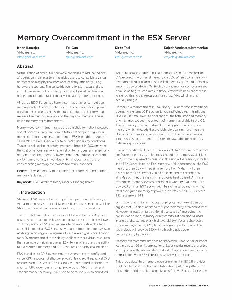
AbstractVirtualization of computer hardware continues to reduce the cost of operation in datacenters. It enables users to consolidate virtual hardware on less physical hardware, thereby efficiently using hardware resources. The consolidation ratio is a measure of the virtual hardware that has been placed on physical hardware. A higher consolidation ratio typically indicates greater efficiency.

VMware’s ESX® Server is a hypervisor that enables competitive memory and CPU consolidation ratios. ESX allows users to power on virtual machines (VMs) with a total configured memory that exceeds the memory available on the physical machine. This is called memory overcommitment.

Memory overcommitment raises the consolidation ratio, increases operational efficiency, and lowers total cost of operating virtual machines. Memory overcommitment in ESX is reliable; it does not cause VMs to be suspended or terminated under any conditions. This article describes memory overcommitment in ESX, analyzes the cost of various memory reclamation techniques, and empirically demonstrates that memory overcommitment induces acceptable performance penalty in workloads. Finally, best practices for implementing memory overcommitment are provided.

General Terms: memory management, memory overcommitment, memory reclamation

Keywords: ESX Server, memory resource management

1. IntroductionVMware’s ESX Server offers competitive operational efficiency of virtual machines (VM) in the datacenter. It enables users to consolidate VMs on a physical machine while reducing cost of operation.

The consolidation ratio is a measure of the number of VMs placed on a physical machine. A higher consolidation ratio indicates lower cost of operation. ESX enables users to operate VMs with a high consolidation ratio. ESX Server’s overcommitment technology is an enabling technology allowing users to achieve a higher consolidation ratio. Overcommitment is the ability to allocate more virtual resources than available physical resources. ESX Server offers users the ability to overcommit memory and CPU resources on a physical machine.

ESX is said to be CPU-overcommitted when the total configured virtual CPU resources of all powered-on VMs exceed the physical CPU resources on ESX. When ESX is CPU-overcommitted, it distributes physical CPU resources amongst powered-on VMs in a fair and efficient manner. Similarly, ESX is said to be memory-overcommitted

when the total configured guest memory size of all powered-on VMs exceeds the physical memory on ESX. When ESX is memory-overcommitted, it distributes physical memory fairly and efficiently amongst powered-on VMs. Both CPU and memory scheduling are done so as to give resources to those VMs which need them most, while reclaiming the resources from those VMs which are not actively using it.

Memory overcommitment in ESX is very similar to that in traditional operating systems (OS) such as Linux and Windows. In traditional OSes, a user may execute applications, the total mapped memory of which may exceed the amount of memory available to the OS. This is memory overcommitment. If the applications consume memory which exceeds the available physical memory, then the OS reclaims memory from some of the applications and swaps it to a swap space. It then distributes the available free memory between applications.

Similar to traditional OSes, ESX allows VMs to power on with a total configured memory size that may exceed the memory available to ESX. For the purpose of discussion in this article, the memory installed in an ESX Server is called ESX memory. If VMs consume all the ESX memory, then ESX will reclaim memory from VMs. It will then distribute the ESX memory, in an efficient and fair manner, to all VMs such that the memory resource is best utilized. A simple example of memory overcommitment is when two 4GB VMs are powered on in an ESX Server with 4GB of installed memory. The total configured memory of powered-on VMs is 2 * 4 = 8GB, while ESX memory is 4GB.

With a continuing fall in the cost of physical memory, it can be argued that ESX does not need to support memory overcommitment. However, in addition to traditional use cases of improving the consolidation ratio, memory overcommitment can also be used in times of disaster recovery, high availability (HA), and distributed power management (DPM) to provide good performance. This technology will provide ESX with a leading edge over contemporary hypervisors.

Memory overcommitment does not necessarily lead to performance loss in a guest OS or its applications. Experimental results presented in this paper with two real-life workloads show gradual performance degradation when ESX is progressively overcommitted.

This article describes memory overcommitment in ESX. It provides guidance for best practices and talks about potential pitfalls. The remainder of this article is organized as follows. Section 2 provides

MeMory overcoMMitMent in the eSX Server

Memory Overcommitment in the ESX ServerIshan Banerjee VMware, Inc. [email protected]

Fei Guo VMware,Inc. [email protected]

Kiran Tati VMware, Inc. [email protected]

Rajesh Venkatasubramanian VMware, Inc. [email protected]

3

VMs are regular processes in KVM2, and therefore standard memory management techniques like swapping apply. For Linux guests, a balloon driver is installed and it is controlled by host via the balloon monitor command. Some hosts also support Kernel Sharedpage Merging (KSM) [1] which works similarly to ESX page sharing. Although KVM presents different memory reclamation techniques, it requires certain hosts and guests to support memory overcommitment. In addition, the management and polices for the interactions among the memory reclamation techniques are missing in KVM.

Xen Server3 uses a mechanism called Dynamic Memory Control (DMC) to implement memory reclamation. It works by proportionally adjusting memory among running VMs based on predefined minimum and maximum memory. VMs generally run with maximum memory, and the memory can be reclaimed via a balloon driver when memory contention in the host occurs. However, Xen does not provide a way to overcommit the host physical memory, hence its consolidation ratio is largely limited. Unlike other hypervisors, Xen provides a transcendent memory management mechanism to manage all host idle memory and guest idle memory. The idle memory is collected into a pool and distributed based on the demand of running VMs. This approach requires the guest OS to be paravirtualized, and only works well for guests with non-concurrent memory pressure.

When compared to existing hypervisors, ESX allows for reliable memory overcommitment to achieve high consolidation ratio with no requirements or modifications for running guests. It implements various memory reclamation techniques to enable overcommitment and manages them in an efficient manner to mitigate possible performance penalties to VMs.

Work on optimal use of host memory in a hypervisor has also been demonstrated by the research community. An optimization for the KSM technique has been attempted in KVM with Singleton [6]. Sub-page level page sharing using patching has been demonstrated in Xen with Difference Engine [2]. Paravirtualized guest and sharing of pages read from storage devices have been shown using Xen in Satori [4].

Memory ballooning has been demonstrated for the z/VM hypervisor using CMM [5]. Ginkgo [3] implements a hypervisor-independent overcommitment framework allowing Java applications to optimize their memory footprint. All these works target specific aspects of memory overcommitment challenges in virtualization environment. They are valuable references for future optimizations in ESX memory management.

Background: Memory overcommitment in ESX is reliable (see Table 1). This implies that VMs will not be prematurely terminated or suspended owing to memory overcommitment. Memory overcommitment in ESX is theoretically limited by the overhead memory of ESX. ESX guarantees reliability of operation under all levels of overcommitment.

background information on memory overcommitment, Section 3 describes memory overcommitment, Section 4 provides quantitative understanding of performance characteristics of memory overcommitment, and Section 5 concludes the article.

2. Background and Related WorkMemory overcommitment enables a higher consolidation ratio in a hypervisor. Using memory overcommitment, users can consolidate VMs on a physical machine such that physical resources are utilized in an optimal manner while delivering good performance. For example in a virtual desktop infrastructure (VDI) deployment, a user may operate many Windows VMs, each containing a word processing application. It is possible to overcommit a hypervisor with such VDI VMs. Since the VMs contain similar OSes and applications, many of their memory pages may contain similar content. The hypervisor will find and consolidate memory pages with identical content from these VMs, thus saving memory. This enables better utilization of memory and enables higher consolidation ratio.

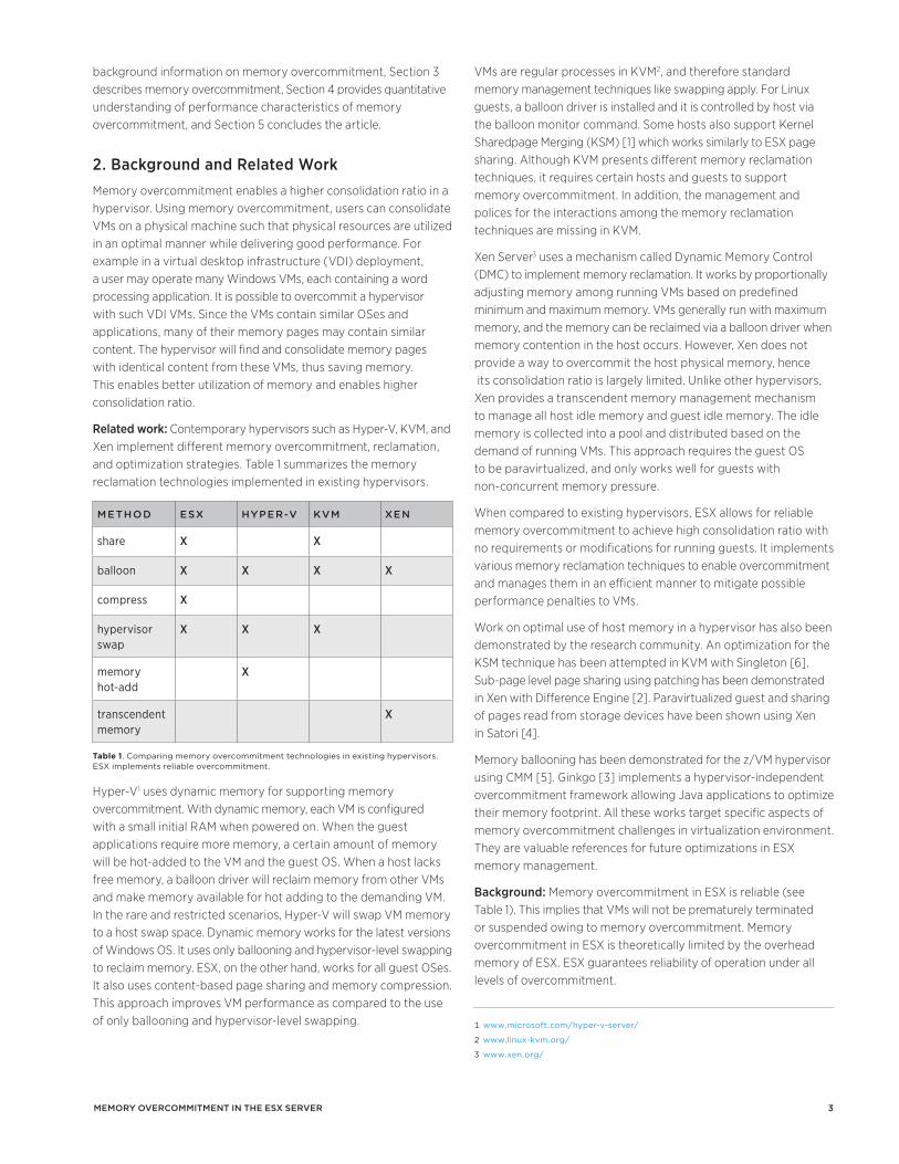
Related work: Contemporary hypervisors such as Hyper-V, KVM, and Xen implement different memory overcommitment, reclamation, and optimization strategies. Table 1 summarizes the memory reclamation technologies implemented in existing hypervisors.

MEthOd ESX hypEr-V KVM XEn

share X X

balloon X X X X

compress X

hypervisor swap

X X X

memory hot-add

X

transcendent memory

X

Table 1. Comparing memory overcommitment technologies in existing hypervisors. ESX implements reliable overcommitment.

Hyper-V1 uses dynamic memory for supporting memory overcommitment. With dynamic memory, each VM is configured with a small initial RAM when powered on. When the guest applications require more memory, a certain amount of memory will be hot-added to the VM and the guest OS. When a host lacks free memory, a balloon driver will reclaim memory from other VMs and make memory available for hot adding to the demanding VM. In the rare and restricted scenarios, Hyper-V will swap VM memory to a host swap space. Dynamic memory works for the latest versions of Windows OS. It uses only ballooning and hypervisor-level swapping to reclaim memory. ESX, on the other hand, works for all guest OSes. It also uses content-based page sharing and memory compression. This approach improves VM performance as compared to the use of only ballooning and hypervisor-level swapping.


1 www.microsoft.com/hyper-v-server/

2 www.linux-kvm.org/

3 www.xen.org/

4

memory page. This method greatly reduces the memory footprint of VMs with common memory content. For example, if an ESX has many VMs executing word processing applications, then ESX may transparently apply page sharing to those VMs and collapse the text and data content of these applications, thereby reducing the footprint of all those VMs. The collapsed memory is freed by ESX and made available for powering on more VMs. This raises the consolidation ratio of ESX and enables higher overcommitment. In addition, if the shared pages are not subsequently written into by the VMs, then they remain shared for a prolonged time, maintaining the reduced footprint of the VM.

Memory ballooning is an active method for reclaiming idle memory from VMs. It is used when ESX is in the soft state. If a VM has consumed memory pages, but is not subsequently using them in an active manner, ESX attempts to reclaim them from the VM using ballooning. In this method, an OS-specific balloon driver inside the VM allocates memory from the OS kernel. It then hands the memory to ESX, which is then free to re-allocate it to another VM which might be actively requiring memory. The balloon driver effectively utilizes the memory management policy of the guest OS to reclaim idle memory pages. The guest OS typically reclaims idle memory inside the guest OS and, if required, swaps them to its own swap space.

When ESX enters the hard state, it actively and aggressively reclaims memory from VMs by swapping out memory to a swap space. During this step, if ESX determines that a memory page is sharable or compressible, then that page is shared or compressed instead. The reclamation done by ESX using swapping is different from that done by the guest OS inside the VM. The guest OS may swap out guest memory pages to its own swap space—for example /swap or pagefile.sys. ESX uses hypervisor-level swapping to reclaim memory from a VM into its own swap space.

The low state is similar to the hard state. In addition to compressing and swapping memory pages, ESX may block certain VMs from allocating memory in this state. It aggressively reclaims memory from VMs, until ESX moves into the hard state.

Page sharing is a passive memory reclamation technique that operates continuously on a powered-on VM. The remaining techniques are active ones that operate when free memory in ESX is low. Also, page sharing, ballooning, and compression are opportunistic techniques. They do not guarantee memory reclamation from VMs. For example, a VM may not have sharable content, the balloon driver may not be installed, or its memory pages may not yield good compression. Reclamation by swapping is a guaranteed method for reclaiming memory from VMs.

In summary, ESX allows for reliable memory overcommitment to achieve a higher consolidation ratio. It implements various memory reclamation techniques to enable overcommitment while improving efficiency and lowering cost of operation of VMs. The next section describes memory overcommitment.

When ESX is memory overcommitted, it allocates memory to those powered-on VMs that need it most and will perform better with more memory. At the same time, ESX reclaims memory from those VMs which are not actively using it. Memory reclamation is therefore an integral component of memory overcommitment. ESX uses different memory reclamation techniques to reclaim memory from VMs. The memory reclamation techniques are transparent page sharing, memory ballooning, memory compression, and memory swapping.

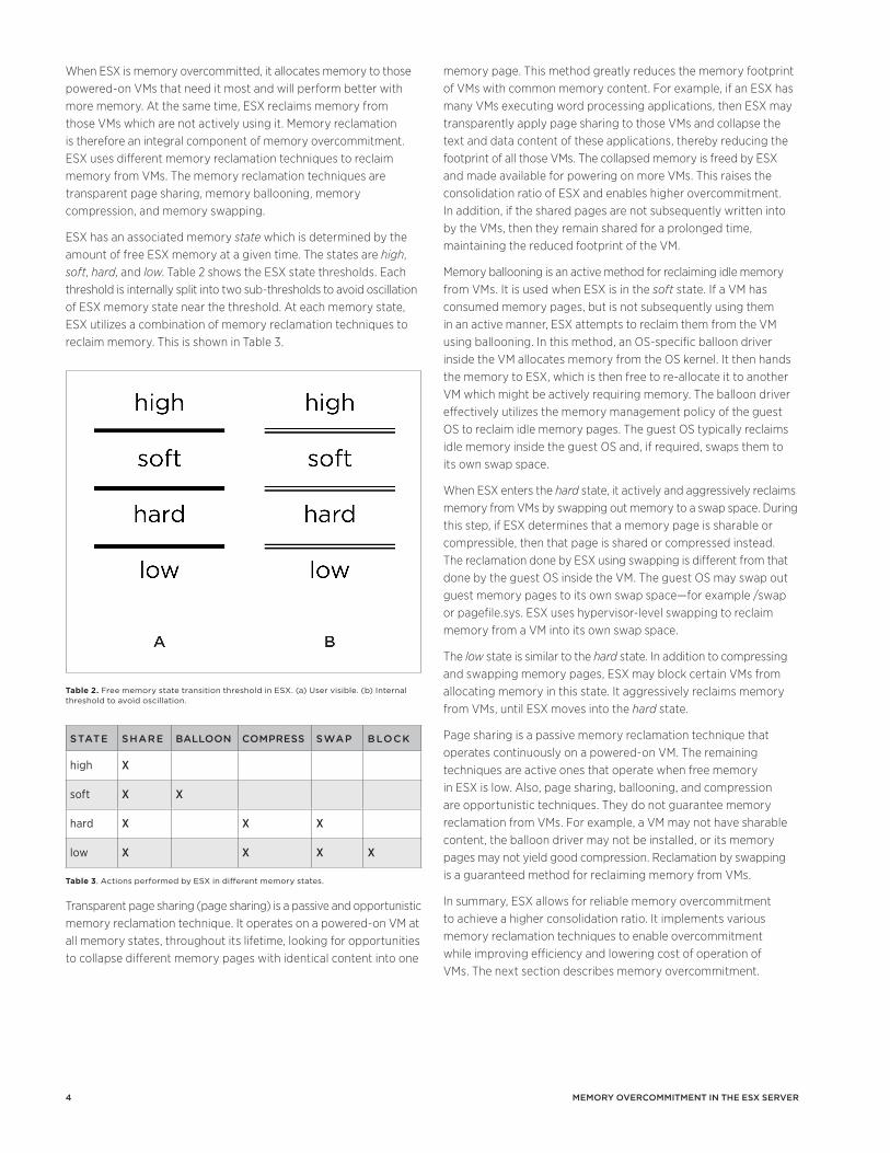
ESX has an associated memory state which is determined by the amount of free ESX memory at a given time. The states are high, soft, hard, and low. Table 2 shows the ESX state thresholds. Each threshold is internally split into two sub-thresholds to avoid oscillation of ESX memory state near the threshold. At each memory state, ESX utilizes a combination of memory reclamation techniques to reclaim memory. This is shown in Table 3.

StatE SharE ballOOn cOMprESS Swap blOcK

high X

soft X X

hard X X X

low X X X X

Table 3. Actions performed by ESX in different memory states.

Transparent page sharing (page sharing) is a passive and opportunistic memory reclamation technique. It operates on a powered-on VM at all memory states, throughout its lifetime, looking for opportunities to collapse different memory pages with identical content into one


Table 2. Free memory state transition threshold in ESX. (a) User visible. (b) Internal threshold to avoid oscillation.

5

ESX also reserves a small amount of memory called minfree. This amount is a buffer against rapid allocations by memory consumers. ESX is in high state as long as there is at least this amount of memory free. If the free memory dips below this value, then ESX is no longer in high state, and it begins to actively reclaim memory.

Figure 1(c) shows the schematic diagram representing an undercommitted ESX when overhead memory is taken into account. In this diagram, the overhead memory consumed by ESX for itself and for each powered-on VM is shown. Figure 1(d) shows the schematic diagram representing an overcommitted ESX when overhead memory is taken into account.

Figure 1(e) shows the theoretical limit of memory overcommitment in ESX. In this case, all of ESX memory is consumed by ESX overhead and per-VM overhead. VMs will be able to power on and boot; however, execution of the VM will be extremely slow.

For simplicity of discussion and calculation, the definition of overcommitment from Figure 1(b) is followed. Overhead memory is ignored for defining memory overcommitment. From this figure:

overcommit = ∑v memsize / ESXmemory (1)

where

overcommit memory overcommitment factor

V powered-on VMs in ESX

memsize configured memory size of v

ESXmemory total installed ESX memory

The representation from this figure is used in the remainder of this article.

To understand memory overcommitment and its effect on VM and applications, mapped, consumed and working set memory are described.

3.2 Mapped MemoryThe definition of memory overcommitment does not consider the memory consumption or memory access characteristic of the powered-on VMs. Immediately after a VM is powered on, it does not have any memory pages allocated to it. Subsequently, as the guest OS boots, the VM access pages in its memory address space ESX overhead by reading or writing into it. ESX allocates physical memory pages to back the virtual address space of the VM during this access. Gradually, as the guest OS completes booting and applications are launched inside the VM, more pages in the virtual address space are backed by physical memory pages. During the lifetime of the ESX overhead VM, the VM may or may not access all pages in its virtual address space.

Windows, for example, writes the zero4 pattern to the complete VM memory address space of the VM. This causes ESX to allocate memory pages for the complete address space by the time Windows has completed booting. On the other hand, Linux does not access the VM memory complete address space of the VM when it boots. It accesses memory pages only required to load the OS.

3. Memory OvercommitmentMemory overcommitment enables a higher consolidation ratio of VMs on an ESX Server. It reduces cost of operation while utilizing compute resources efficiently. This section describes memory overcommitment and its performance characteristics.

3.1 DefinitionsESX is said to be memory overcommitted when VMs are powered on such that their total configured memory size is greater than ESX memory. Figure 1 shows an example of memory overcommitment on ESX.

Figure 1(a) shows the schematic diagram of a memory-undercommitted ESX Server. In this example, ESX memory is 4GB. Two VMs, each with a configured memory size of 1GB, are powered on. The total configured memory size of powered-on VMs is therefore 2GB, which is less than 4GB. Hence ESX is considered to be memory undercommitted.

Figure 1(b) shows the schematic diagram of a memory-overcommitted ESX Server. In this example, ESX memory is 4GB. Three VMs, with configured memory sizes of 1GB, 2.5GB and 1GB, are powered on. The total configured memory size of powered-on VMs is therefore 4.5GB which is more than 4GB. Hence ESX is considered to be memory overcommitted.

The scenarios described above omit the memory overhead consumed by ESX. ESX consumes a fixed amount of memory for its own text and data structures. In addition, it consumes overhead memory for each powered-on VM.


Figure 1. Memory overcommitment shown with and without overhead memory. (a) Undercommitted ESX. (b) Overcommitted ESX. This model is typically followed when describing overcommitment. (c) Undercommitted ESX shown with overhead memory. (d) Overcommitted ESX shown with overhead memory. (e) Limit of memory overcommitment.

4 A memory page with all 0x00 content is a zero page.

6

All memory pages of a VM which are ever accessed by a VM are considered mapped by ESX. A mapped memory pages is backed by a physical memory page by ESX during the very first access by the VM. A mapped page may subsequently be reclaimed by ESX. It is considered as mapped through the lifetime of the VM.

When ESX is overcommitted, the total mapped pages by all VMs may or may not exceed ESX memory. Hence, it is possible for ESX to be memory overcommitted, but at the same time, owing to the nature of the guest OS and its applications, the total mapped memory remain within ESX memory. In such a scenario, ESX does not actively reclaim memory from VMs and VMs performance are not affected by memory reclamation.

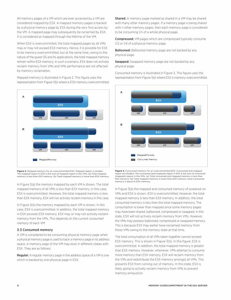
Mapped memory is illustrated in Figure 2. This figure uses the representation from Figure 1(b) where is ESX memory overcommitted.

In Figure 2(a) the memory mapped by each VM is shown. The total mapped memory of all VMs is less than ESX memory. In this case, ESX is overcommitted. However, the total mapped memory is less than ESX memory. ESX will not actively reclaim memory in this case.

In Figure 2(b) the memory mapped by each VM is shown. In this case, ESX is overcommitted. In addition, the total mapped memory in ESX exceeds ESX memory. ESX may or may not actively reclaim memory from the VMs. This depends on the current consumed memory of each VM.

3.3 Consumed memoryA VM is considered to be consuming physical memory page when a physical memory page is used to back a memory page in its address space. A memory page of the VM may exist in different states with ESX. They are as follows:

Regular: A regular memory page in the address space of a VM is one which is backed by one physical page in ESX.

Shared: A memory page marked as shared in a VM may be shared with many other memory pages. If a memory page is being shared with n other memory pages, then each memory page is considered to be consuming 1/n of a whole physical page.

Compressed: VM pages which are compressed typically consume 1/2 or 1/4 of a physical memory page.

Ballooned: Ballooned memory page are not backed by any physical page.

Swapped: Swapped memory page are not backed by any physical page.

Consumed memory is illustrated in Figure 3. This figure uses the representation from Figure 1(b) where ESX is memory overcommitted.

In Figure 3(a) the mapped and consumed memory of powered-on VMs and ESX is shown. ESX is overcommitted. However, the total mapped memory is less than ESX memory. In addition, the total consumed memory is less than the total mapped memory. The consumption is lower than mapped since some memory pages may have been shared, ballooned, compressed or swapped. In this state, ESX will not actively reclaim memory from VMs. However, the VMs may possess ballooned, compressed or swapped memory. This is because ESX may earlier have reclaimed memory from these VMs owing to the memory state at that time.

The total consumption of all VMs taken together cannot exceed ESX memory. This is shown in Figure 3(b). In this figure, ESX is overcommitted. In addition, the total mapped memory is greater than ESX memory. However, whenever, VMs attempt to consume more memory than ESX memory, ESX will reclaim memory from the VMs and redistribute the ESX memory amongst all VMs. This prevents ESX from running out of memory. In this state, ESX is likely going to actively reclaim memory from VMs to prevent memory exhaustion.


Figure 2. Mapped memory for an overcommitted ESX. Mapped region is shaded. The mapped region in ESX is the sum of mapped region in the VMs. (a) Total mapped memory is less than ESX memory. (b) Total mapped memory is more than ESX memory.

Figure 3. Consumed memory for an overcommitted ESX. Consumed and mapped region are shaded. The consumed (and mapped) region in ESX is the sum of consumed (mapped) region in the VMs. (a) Total consumed and mapped memory is less than ESX memory. (b) Total mapped memory is more than ESX memory, total consumed memory is equal to ESX memory.

7

3.4 Working SetThe working set of a VM is the set of memory pages which are being “actively” accessed by the VM. The size of the working set depends on the precise definition of “active”. A precise definition is being omitted in this article since it requires analysis and discussion beyond the scope of this article. The working set of a VM depends on the application it is executing and its memory access characteristics. The working set may change slowly in size and location for some applications while for other applications, the change may be rapid.

Memory pages in a working set are either shared pages or regular pages. If the working set accesses a compressed, ballooned or swapped page or writes into a shared page, then that page will be page-faulted and immediately backed by a physical page by ESX. This page-fault incurs a temporal cost. The temporal cost is typically high for pages swapped onto a spinning disk. This high cost of page-fault may cause the VM to be temporarily stalled. This in turn adversely affects the performance of the VM and its applications.

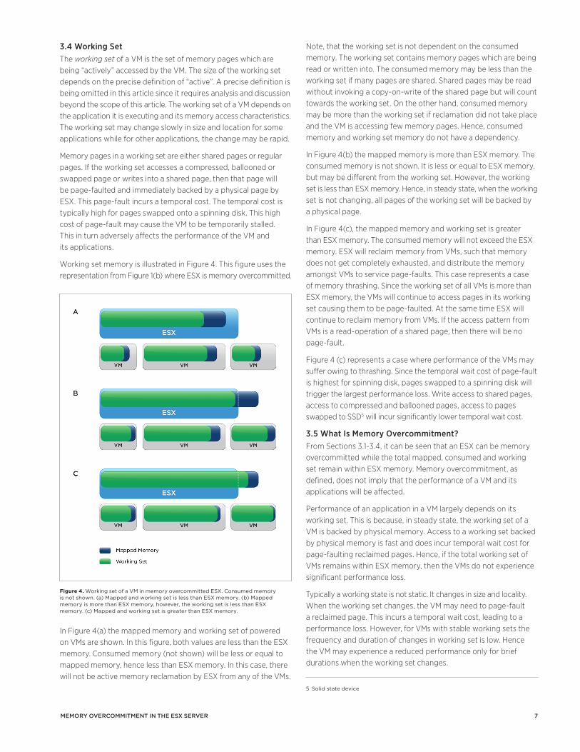
Working set memory is illustrated in Figure 4. This figure uses the representation from Figure 1(b) where ESX is memory overcommitted.

In Figure 4(a) the mapped memory and working set of powered on VMs are shown. In this figure, both values are less than the ESX memory. Consumed memory (not shown) will be less or equal to mapped memory, hence less than ESX memory. In this case, there will not be active memory reclamation by ESX from any of the VMs.

Note, that the working set is not dependent on the consumed memory. The working set contains memory pages which are being read or written into. The consumed memory may be less than the working set if many pages are shared. Shared pages may be read without invoking a copy-on-write of the shared page but will count towards the working set. On the other hand, consumed memory may be more than the working set if reclamation did not take place and the VM is accessing few memory pages. Hence, consumed memory and working set memory do not have a dependency.

In Figure 4(b) the mapped memory is more than ESX memory. The consumed memory is not shown. It is less or equal to ESX memory, but may be different from the working set. However, the working set is less than ESX memory. Hence, in steady state, when the working set is not changing, all pages of the working set will be backed by a physical page.

In Figure 4(c), the mapped memory and working set is greater than ESX memory. The consumed memory will not exceed the ESX memory. ESX will reclaim memory from VMs, such that memory does not get completely exhausted, and distribute the memory amongst VMs to service page-faults. This case represents a case of memory thrashing. Since the working set of all VMs is more than ESX memory, the VMs will continue to access pages in its working set causing them to be page-faulted. At the same time ESX will continue to reclaim memory from VMs. If the access pattern from VMs is a read-operation of a shared page, then there will be no page-fault.

Figure 4 (c) represents a case where performance of the VMs may suffer owing to thrashing. Since the temporal wait cost of page-fault is highest for spinning disk, pages swapped to a spinning disk will trigger the largest performance loss. Write access to shared pages, access to compressed and ballooned pages, access to pages swapped to SSD5 will incur significantly lower temporal wait cost.

3.5 What Is Memory Overcommitment?From Sections 3.1-3.4, it can be seen that an ESX can be memory overcommitted while the total mapped, consumed and working set remain within ESX memory. Memory overcommitment, as defined, does not imply that the performance of a VM and its applications will be affected.

Performance of an application in a VM largely depends on its working set. This is because, in steady state, the working set of a VM is backed by physical memory. Access to a working set backed by physical memory is fast and does incur temporal wait cost for page-faulting reclaimed pages. Hence, if the total working set of VMs remains within ESX memory, then the VMs do not experience significant performance loss.

Typically a working state is not static. It changes in size and locality. When the working set changes, the VM may need to page-fault a reclaimed page. This incurs a temporal wait cost, leading to a performance loss. However, for VMs with stable working sets the frequency and duration of changes in working set is low. Hence the VM may experience a reduced performance only for brief durations when the working set changes.


Figure 4. Working set of a VM in memory overcommitted ESX. Consumed memory is not shown. (a) Mapped and working set is less than ESX memory. (b) Mapped memory is more than ESX memory, however, the working set is less than ESX memory. (c) Mapped and working set is greater than ESX memory.

5 Solid state device

8

Page-fault cost: When a shared page is read by a VM, it is accessed by the VM in a read-only manner. Hence that shared pages does not need to be page-faulted. Hence there is no page-fault cost. A write access to a shared page incurs a cost.

CPU. When a shared page is written to, by a VM, ESX must allocate a new page and replicate the shared content before allowing the write access from the VM. This allocation incurs a CPU cost. Typically, this cost is very low and does not significantly affect VM applications and benchmarks.

Wait. The copy-on-write operation when a VM accesses a shared page with write access is fairly fast. VM applications accessing the page do not incur noticeable temporal cost.

b) Ballooning Reclamation cost: Memory is ballooned from a VM using a balloon driver residing inside the guest OS. When the balloon driver expands, it may induce the guest OS to reclaim memory from guest applications.

CPU. Ballooning incurs a CPU cost on a per-VM basis since it induces memory allocation and reclamation inside the VM.

Storage. The guest OS may swap out memory pages to the guest swap space. This incurs storage space and storage bandwidth cost.

Page-fault cost: CPU. A ballooned page acquired by the balloon driver may subsequently be released by it. The guest OS or application may then allocate and access it. This incurs a page-fault in the guest OS as well as ESX. The page-fault incurs a low CPU cost since a memory page simply needs to be allocated.

Storage. During reclamation by ballooning, application pages may have been swapped out by the guest OS. When the application attempts to access that page, the guest OS needs to swap it in. This incurs a storage bandwidth cost.

Wait. A temporal wait cost may be incurred by application if its pages were swapped out by the guest OS. The wait cost of swapping in a memory page by the guest OS incurs a smaller overall wait cost to the application than a hypervisor-level swap-in. This is because during a page fault in the guest OS, by one thread, the guest OS may schedule another thread. However, if ESX is swapping in a page, then it may deschedule the entire VM. This is because ESX cannot reschedule guest OS threads.

c) Compression Reclamation cost: Memory is compressed in a VM by compressing a full guest memory page such that is consumes 1/2 or 1/4 physical memory page. There is effectively no memory cost, since every successful compression releases memory.

CPU. A CPU cost is incurred for every attempted compression. The CPU cost is typically low and is charged to the VM whose memory is being compressed. The CPU cost is however, more than that for page sharing. It may lead to noticeably reduced VM performance and may affect benchmarks.

3.6 Cost of Memory OvercommitmentMemory overcommitment incurs certain cost in terms of compute resource as well as VM performance. This section provides a qualitative understanding of the different sources of cost and their magnitude.

When ESX is memory overcommitted and powered-on VMs attempt to consume more memory than ESX memory, then ESX will begin to actively reclaim memory from VMs. Hence memory reclamation is an integral component of memory overcommitment.

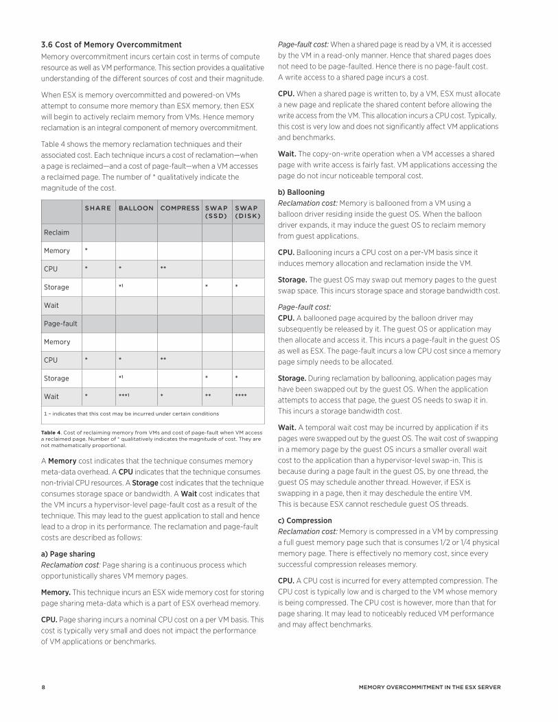
Table 4 shows the memory reclamation techniques and their associated cost. Each technique incurs a cost of reclamation—when a page is reclaimed—and a cost of page-fault—when a VM accesses a reclaimed page. The number of * qualitatively indicate the magnitude of the cost.

SharE ballOOn cOMprESS Swap (SSd)

Swap (diSK)

Reclaim

Memory *

CPU * * **

Storage *1 * *

Wait

Page-fault

Memory

CPU * * **

Storage *1 * *

Wait * ***1 * ** ****

1 – indicates that this cost may be incurred under certain conditions

Table 4. Cost of reclaiming memory from VMs and cost of page-fault when VM access a reclaimed page. Number of * qualitatively indicates the magnitude of cost. They are not mathematically proportional.

A Memory cost indicates that the technique consumes memory meta-data overhead. A CPU indicates that the technique consumes non-trivial CPU resources. A Storage cost indicates that the technique consumes storage space or bandwidth. A Wait cost indicates that the VM incurs a hypervisor-level page-fault cost as a result of the technique. This may lead to the guest application to stall and hence lead to a drop in its performance. The reclamation and page-fault costs are described as follows:

a) Page sharing Reclamation cost: Page sharing is a continuous process which opportunistically shares VM memory pages.

Memory. This technique incurs an ESX wide memory cost for storing page sharing meta-data which is a part of ESX overhead memory.

CPU. Page sharing incurs a nominal CPU cost on a per VM basis. This cost is typically very small and does not impact the performance of VM applications or benchmarks.


9

4. PerformanceThis section provides a quantitative demonstration of memory overcommitment in ESX. Simple applications are shown to work using memory overcommitment. This section does not provide a comparative analysis using software benchmarks.

4.1 MicrobenchmarkThis set of experiment was conducted on a development build of ESX 6.0. The ESX Server has 32GB RAM, 4 quad-core AMD CPU configured in a 4-NUMA node configuration. The VMs used in the experiments are 2-vCPU, 24GB and contain RHEL6 OS. The ESX Server consumes about 4 GB memory—ESX memory overhead, per-VM memory overhead, reserved minfree. This gives about 28GB for allocating to VMs. For these experiments, ESX memory is 32GB. However, ESX will actively reclaim memory from VMs when VMs consume more than 28GB (available ESX memory). RHEL6 consumes about 1GB memory when booted and idle. This will contribute to the mapped and consumed memory of the VM.

These experiments demonstrate performance of VMs when the total working set varies compared to available ESX memory. Figure 5 shows the results from three experiments. For the purpose of demonstration and simplicity the three reclamation techniques—page sharing, ballooning and compression—are disabled. Hypervisor-level memory swapping is the only active memory reclamation technique in this experiment. This reclamation will start when VMs consumed more than available ESX memory.

In these experiments, presence of hypervisor-level page-fault is an indicator of performance loss. Figures show cumulative swap-in (page-fault) values. When this value rises, VM will experience temporal wait cost. When it does not rise, there is no temporal wait cost and hence no performance loss.

Experiment a: In Figure 5(a) an experiment is conducted similar to Figure 4(a). In this experiment, the total mapped and total working set memory always remain less than available ESX memory.

Page-fault cost: When a compressed memory page is accessed by the VM, ESX must allocate a new page and de-compress the page before allowing access to the VM.

CPU. De-compression incurs a CPU cost.

Wait. The VM also waits until the page is de-compressed. This is typically not very high since the de-compression takes place in-memory.

d) Swap Reclamation cost: ESX swaps out memory pages from a VM to avoid memory exhaustion. The swap-out process takes place asynchronous to the execution of the VM and its application. Hence, the VM and its applications do not incur a temporal wait cost.

Storage. Swapping out memory pages from a VM incurs storage space and storage bandwidth cost.

Page-fault cost: When a VM page-faults a swapped page, ESX must read the page from the swap space synchronously before allowing the VM to access the page.

Storage. This incurs a storage bandwidth cost.

Wait. The VM also incurs a temporal wait cost while the swapped page is synchronously read from storage device. The temporal wait cost is highest for a swap space located on spinning disk. Swap space located on SSD incurs lower temporal wait cost.

The cost of reclamation and page-fault vary significantly between different reclamation techniques. Reclamation by ballooning may incur a storage cost only in certain cases. Reclamation by swapping always incurs storage cost. Similarly, page-fault owing to reclamation incurs a temporal wait cost in all cases. Page-fault of a swapped page incurs the highest temporal wait cost. Table 4 shows the cost of reclamation as well as the cost of page-fault incurred by a VM on a reclaimed memory page.

The reclamation itself does not impact VM and application performance significantly, since the temporal wait cost of reclamation is zero for all techniques. Some techniques have a low CPU cost. This cost may be charged to the VM leading to slightly reduced performance6.

However, during page-fault temporal wait cost exists for all techniques. This affects VM and application performance. Write access to shared page, access to compressed, ballooned pages incur the least performance cost. Access to swapped page, specially pages swapped to spinning disk, incurs the highest performance cost.

Section 3 described memory overcommitment in ESX. It defined various terms — mapped, consumed, working set memory — and showed its relation to memory overcommitment. It also showed that memory overcommitment does not necessarily impact VM and application performance. It also provided a qualitative analysis of how memory overcommitment may impact VM and application performance depending on the VM’s memory content and access characteristics.

The next section provides quantitative description of overcommitment.


6 CPU cost of reclamation may affect performance only if ESX is operating at 100% CPU load

Figure 5. Effect of working set of memory reclamation and page-fault. Available ESX memory=28GB. (a) mapped, working set < available ESX memory. (b) mapped > available ESX memory, working set < available ESX memory. (c) mapped, working set > available ESX memory.

1 0

Two VMs each of configured memory size 24GB are powered on. The overcommitment factor is 1.5. Each VM runs a workload. Each workload allocates 15GB memory and writes a random pattern into it. It then reads all 15GB memory continuously in a round robin manner for 2 iterations. The memory mapped by each VM is about 16GB (workload=15GB, RHEL6=1GB), the total being 32GB. The working set is also 32GB. Both exceed available ESX memory.

The figure shows mapped memory for each VM and cumulative swap-in. The X-axis in this figure shows time in seconds, Y-axis (left) shows mapped memory in MB and Y-axis (right) shows cumulative swap-in. It can be seen from this figure that a steady page-fault is maintained once the workloads have mapped the target memory. This indicates that as the workloads are accessing memory, they are experiencing page-faults. ESX is continuously reclaiming memory from each VM as the VM page-faults its working set.

This experiment demonstrates that workloads will experience steady page-faults and hence performance loss when the working set exceeds available ESX memory. Note that if the working set read-accesses shared pages and page sharing is enabled (default ESX behavior) then a page-fault is avoided.

In this section experiments were designed to highlight the basic working of overcommitment. In these experiments, page sharing, ballooning and compression were disabled for simplicity. These reclamation techniques reclaim memory effectively before reclamation by swapping can take place. Since page faults to shared, ballooned and compressed memory have a lower temporal wait cost, the workload performance is better. This will be demonstrated in the next section.

4.2 Real WorkloadsIn this section, the experiments are conducted using vSphere 6.0. The ESX Server has 72GB RAM, 4 quad-core AMD CPU. The workloads used to evaluate memory overcommitment performance are DVDstore27 and a VDI workload. Experiments were conducted with default memory management configurations for pshare, balloon and compression.

Experiment d: The DVDstore2 workload simulates online database operations for ordering DVDs. In this experiment, 5 DVDstore2 VMs are used, each configured with 4 vCPUs and 4GB memory. It contains Windows Server 2008 OS and SQL Server 2008. The performance metric is the total operations per minute of all 5 VMs.

Since 5-4GB VMs are used, the total memory size of all powered-on VMs is 20GB. However, the ESX Server contains 72GB installed RAM and was effectively undercommitted. Hence, memory overcommitment was simulated with the use of a memory hog VM. The memory hog VM had full memory reservation. Its configured memory size was progressively increased in each run. This effectively reduced the ESX memory available to the DVDStore2 VMs.

Two VMs each of configured memory size 24GB are powered on. Since ESX memory is 32GB, the overcommitment factor is (2 * 24) / 32 = 1.5. Each VM executes an identical hand-crafted workload. The workload is a memory stress program. It allocates 12GB memory, writes random pattern into all of this allocated memory and continuously reads this memory in a round-robin manner. This workload is executed in both VMs. Hence a total of 24GB memory is mapped and actively used by the VMs. The workload is executed for 900 seconds.

The figure shows mapped memory for each VM. It also shows the cumulative swap-in for each VM. The X-axis in this figure shows time in seconds, Y-axis (left) shows mapped memory in MB and Y-axis (right) shows cumulative swap-in. The memory mapped by each VM is about 13GB (workload=12GB, RHEL6=1GB), the total being 26GB. This is less than available ESX memory. It can be seem from this figure that there is no swap-in (page-fault) activity at any time. Hence there is no performance loss. The memory mapped by the VMs rise as the workload allocates memory. Subsequently, as the workload accesses the memory in a round-robin manner, all of the memory is backed by physical memory pages by ESX.

This experiment demonstrates that although memory is overcommitted, VMs mapping and actively using less than available ESX memory will not be subjected to active memory reclamation and hence will not experience any performance loss.

Experiment b: In Figure 5(b) an experiment is conducted similar to Figure 4(b). In this experiment, the total mapped memory exceeds available ESX memory while the total working set memory is less than available ESX memory.

Two VMs each of configured memory size 24GB are powered on. The resulting memory overcommitment is 1.5. The workload in each VM allocates 15GB of memory and writes a random pattern into it. It then reads a fixed block, 12.5% of 15GB (=1.875GB) in size, from this 15GB in a round-robin manner for 2 iterations. Thereafter, the same fixed block is read in a round-robin manner for 10,000 seconds. This workload is executed in both VMs. The memory mapped by each VM is about 16GB (workload=15GB, RHEL=1GB), the total being 32GB. This exceeds available ESX memory. The working set is thereafter a total of 2 * 1.875 = 3.75GB.

The figure shows mapped memory for each VM and cumulative swap-in. The X-axis in this figure shows time in seconds, Y-axis (left) shows mapped memory in MB and Y-axis (right) shows cumulative swap-in. It can be seen from this figure that as the workload maps memory, the mapped memory rises. Thereafter, there is an initial rising swap-in activity as the working set is page-faulted. After the working set is page-faulted, the cumulative swap-in is steady.

This experiment demonstrates that although memory is overcommitted and VMs have mapped more memory than available ESX memory, VMs will perform better when its working set is smaller than available ESX memory.

Experiment c: In Figure 5(c) an experiment is conducted similar to Figure 4(c). In this experiment, the total mapped memory as well as the total working set exceeds available ESX memory.


7 http://en.community.dell.com/techcenter/extras/w/wiki/dvd-store.aspx

1 1

In this experiment, 15 VDI VMs are powered-on in the ESX Server. Each VM is configured with 1 vCPU and 4GB memory—the total configured memory size of all VMs being 15 * 4 = 60GB. The VMs contain Windows7 OS. Similar to experiment d, a memory hog VM, with full memory reservation, is used to simulate overcommitment by effectively reducing the ESX memory on the ESX Server.

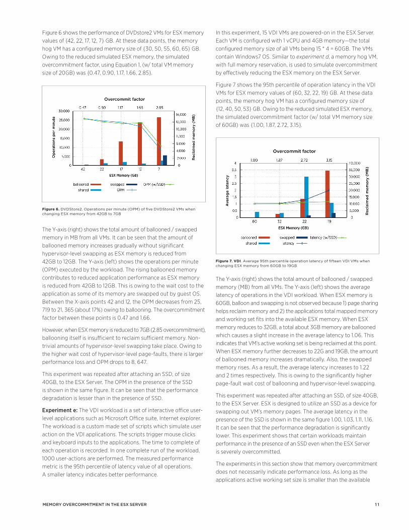
Figure 7 shows the 95th percentile of operation latency in the VDI VMs for ESX memory values of {60, 32, 22, 19} GB. At these data points, the memory hog VM has a configured memory size of {12, 40, 50, 53} GB. Owing to the reduced simulated ESX memory, the simulated overcommitment factor (w/ total VM memory size of 60GB) was {1.00, 1.87, 2.72, 3.15}.

The Y-axis (right) shows the total amount of ballooned / swapped memory (MB) from all VMs. The Y-axis (left) shows the average latency of operations in the VDI workload. When ESX memory is 60GB, balloon and swapping is not observed because 1) page sharing helps reclaim memory and 2) the applications total mapped memory and working set fits into the available ESX memory. When ESX memory reduces to 32GB, a total about 3GB memory are ballooned which causes a slight increase in the average latency to 1.06. This indicates that VM’s active working set is being reclaimed at this point. When ESX memory further decreases to 22G and 19GB, the amount of ballooned memory increases dramatically. Also, the swapped memory rises. As a result, the average latency increases to 1.22 and 2 times respectively. This is owing to the significantly higher page-fault wait cost of ballooning and hypervisor-level swapping.

This experiment was repeated after attaching an SSD, of size 40GB, to the ESX Server. ESX is designed to utilize an SSD as a device for swapping out VM’s memory pages. The average latency in the presence of the SSD is shown in the same figure 1.00, 1.03, 1.11, 1.16. It can be seen that the performance degradation is significantly lower. This experiment shows that certain workloads maintain performance in the presence of an SSD even when the ESX Server is severely overcommitted.

The experiments in this section show that memory overcommitment does not necessarily indicate performance loss. As long as the applications active working set size is smaller than the available

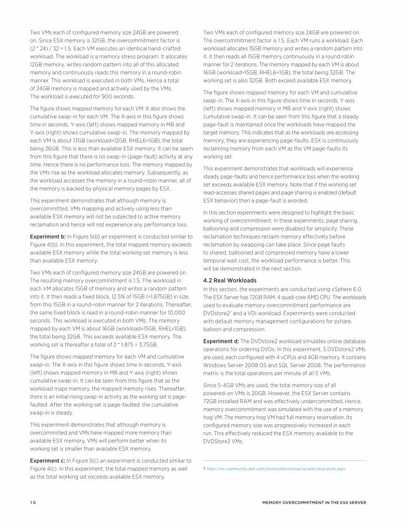
Figure 6 shows the performance of DVDstore2 VMs for ESX memory values of {42, 22, 17, 12, 7} GB. At these data points, the memory hog VM has a configured memory size of {30, 50, 55, 60, 65} GB. Owing to the reduced simulated ESX memory, the simulated overcommitment factor, using Equation 1, (w/ total VM memory size of 20GB) was {0.47, 0.90, 1.17, 1.66, 2.85}.

The Y-axis (right) shows the total amount of ballooned / swapped memory in MB from all VMs. It can be seen that the amount of ballooned memory increases gradually without significant hypervisor-level swapping as ESX memory is reduced from 42GB to 12GB. The Y-axis (left) shows the operations per minute (OPM) executed by the workload. The rising ballooned memory contributes to reduced application performance as ESX memory is reduced from 42GB to 12GB. This is owing to the wait cost to the application as some of its memory are swapped out by guest OS. Between the X-axis points 42 and 12, the OPM decreases from 25, 719 to 21, 365 (about 17%) owing to ballooning. The overcommitment factor between these points is 0.47 and 1.66.

However, when ESX memory is reduced to 7GB (2.85 overcommitment), ballooning itself is insufficient to reclaim sufficient memory. Non-trivial amounts of hypervisor-level swapping take place. Owing to the higher wait cost of hypervisor-level page-faults, there is larger performance loss and OPM drops to 8, 647.

This experiment was repeated after attaching an SSD, of size 40GB, to the ESX Server. The OPM in the presence of the SSD is shown in the same figure. It can be seen that the performance degradation is lesser than in the presence of SSD.

Experiment e: The VDI workload is a set of interactive office user-level applications such as Microsoft Office suite, Internet explorer. The workload is a custom made set of scripts which simulate user action on the VDI applications. The scripts trigger mouse clicks and keyboard inputs to the applications. The time to complete of each operation is recorded. In one complete run of the workload, 1000 user-actions are performed. The measured performance metric is the 95th percentile of latency value of all operations. A smaller latency indicates better performance.


Figure 6. DVDStore2. Operations per minute (OPM) of five DVDStore2 VMs when changing ESX memory from 42GB to 7GB

Figure 7. VDI. Average 95th percentile operation latency of fifteen VDI VMs when changing ESX memory from 60GB to 19GB

1 2

References1 A. Arcangeli, I. Eidus, and C. Wright. Increasing memory

density by using KSM. In Proceedings of the Linux Symposium, pages 313—328, 2009.

2 D. Gupta, S. Lee, M. Vrable, S. Savage, A. C. Snoeren, G. Varghese, G. M. Voelker, and A. Vahdat. Difference engine: harnessing memory redundancy in virtual machines. Commun. ACM, 53(10):85-93, Oct. 2010.

3 M. Hines, A. Gordon, M. Silva, D. Da Silva, K. D. Ryu, and M. BenYehuda. Applications Know Best: Performance-Driven Memory Overcommit with Ginkgo. In Cloud Computing Technology and Science (CloudCom), 2011 IEEE Third International Conference on, pages 130-137, 2011.

4 G. Milos, D. Murray, S. Hand, and M. Fetterman. Satori: Enlightened o page sharing. In Proceedings of the 2009 conference on USENIX Annual technical conference. USENIX Association, 2009.

5 M. Schwidefsky, H. Franke, R. Mansell, H. Raj, D. Osisek, and J. Choi. Collaborative Memory Management in Hosted Linux Environments. In Proceedings of the Linux Symposium, pages 313-328, 2006.

6 P. Sharma and P. Kulkarni. Singleton: system-wide page deduplication in virtual environments. In Proceedings of the 21st international symposium on High-Performance Parallel and Distributed Computing, HPDC ‘12, pages 15-26, New York, NY, USA, 2012. ACM.

7 C. A. Waldspurger. Memory resource management in VMware ESX server. SIGOPS Oper. Syst. Rev., 36(SI):181-194, Dec. 2002.

ESX memory, the performance degradation may be tolerable. In many situations where memory is slightly or moderately overcommitted, page sharing and ballooning is able to reclaim memory gracefully without significantly performance penalty. However, under high memory overcommitment hypervisor-level swapping may occur, leading to significant performance degradation.

5. ConclusionReliable memory overcommitment is a unique capability of ESX, not present in any contemporary hypervisor. Using memory overcommitment, ESX can power on VMs such that the total configured memory of all powered-on VMs exceed ESX memory. ESX distributes memory between all VMs in a fair and efficient manner so as to maximize utilization of the ESX Server. At the same time memory overcommitment is reliable. This means that VMs will not be prematurely terminated or suspended owing to memory overcommitment. Memory reclamation techniques of ESX guarantees safe operation of VMs in a memory overcommitted environment.

6. AcknowledgmentsMemory overcommitment in ESX was designed and implemented by Carl Waldspurger [7].


1 3

1. IntroductionTraditionally, storage arrays were built of spinning disks with a few gigabytes of battery-backed NVRAM as local cache. The typical I/O response time was multiple milliseconds, and the maximum supported IOPS were a few thousand. Today in the flash era, arrays are advertising I/O latencies of under a millisecond and IOPS on the order of millions. XtremIO [20] (now EMC), Violin Memory [16], WhipTail [18], Nimbus [7], Solid-Fire [22], PureStorage [14], Nimble [13], GridIron (now Violin) [23], CacheIQ (now NetApp) [21], and Avere Systems [11] are some of the emerging startups developing storage solutions that leverage flash. Additionally, established players (namely EMC, IBM, HP, Dell, and NetApp) are also actively developing solutions. Flash is also being adopted within servers as a flash cache to accelerate I/Os by serving them locally—some of the example solutions include [8, 10, 17, 24]. Given the current trends, it is expected that all-flash and hybrid arrays will completely replace the traditional disk-based arrays by the end of this decade. To summarize, the I/O saturation bottleneck is now shifting—administrators are no longer worried about how many requests the array can service, but rather how fast the server can be configured to send these I/O requests and utilize the bandwidth.

Multipathing is a mechanism for a server to connect to a storage array using multiple available fabric ports. ESXi’s multipathing logic is implemented as a Path Selection Plug-in (PSP) within the PSA (Pluggable Storage Architecture) layer [12]. The ESXi product today ships with three different multipathing algorithms as a NMP (Native Multipathing Plug-in) framework: PSP FIXED, PSP MRU, and PSP RR. Both PSP FIXED and PSP MRU utilize only one fixed path for I/O requests and do not perform any load balancing, while PSP RR does a simple round-robin load balancing among all Active Optimized paths. Also, there are commercial solutions available (as described in the related work section) that essentially differ in how they distribute load across the Active Optimized paths.

In this paper, we explore a novel idea of using both Active Optimized and Un-optimized paths concurrently. Active Un-optimized paths have traditionally been used only for failover scenarios, since these paths are known to exhibit a higher service time compared to Active Optimized paths. The hypothesis of our approach was that the service times were high, since the contention bottleneck is the array bandwidth, limited by the disk IOPS. In the new flash era, the array is far from being a hardware bottleneck. We discovered that our hypothesis is half true, and we designed a plug-in solution around it called PSP Adaptive.

AbstractAt the advent of virtualization, primary storage equated spinning disks. Today, the enterprise storage landscape is rapidly changing with low-latency all-flash storage arrays, specialized flash-based I/O appliances, and hybrid arrays with built-in flash. Also, with the adoption of host-side flash cache solutions (similar to vFlash), the read-write mix of operations emanating from the server is more write-dominated (since reads are increasingly served locally from cache). Is the original ESXi I/O multipathing logic that was developed for disk-based arrays still applicable in this new flash storage era? Are there optimizations we can develop as a differentiator in the vSphere platform for supporting this core functionality?

This paper argues that existing I/O multipathing in ESXi is not the most optimal for flash-based arrays. In our evaluation, the maximum I/O throughput is not bound by a hardware resource bottleneck, but rather by the Pluggable Storage Architecture (PSA) module that implements the multipathing logic. The root cause is the affinity maintained by the PSA module between the host traffic and a subset of the ports on the storage array (referred to as Active Optimized paths). Today, the Active Un-optimized paths are used only during hardware failover events, since un-optimized paths exhibit higher service time than optimized paths. Thus, even though the Host Bus Adaptor (HBA) hardware is not completely saturated, we are artificially constrained in software by limiting to the Active Optimized paths only.

We implemented a new multipathing approach called PSP Adaptive as a Path-Selection Plug-in in the PSA. This approach detects I/O path saturation (leveraging existing SIOC techniques), and spreads the write operations across all the available paths (optimized and un-optimized), while reads continue to maintain their affinity paths. The key observation was that the higher service times in the un-optimized paths are still lower than the wait times in the optimized paths. Further, read affinity is important to maintain given the session-based prefetching and caching semantics used by the storage arrays. During periods of non-saturation, our approach switches to the traditional affinity model for both reads and writes. In our experiments, we observed significant (up to 30%) improvements in throughput for some workload scenarios. We are currently in the process of working with a wide range of storage partners to validate this model for various Asymmetric Logical Units Access (ALUA) storage implementations and even Metro Clusters.

redefining ESXi iO Multipathing in the Flash EraFei Meng North Carolina State University [email protected]

Li Zhou1 Facebook Inc. [email protected]

Sandeep Uttamchandani VMware, Inc. [email protected]

Xiaosong Ma North Carolina State University & Oak Ridge National Lab [email protected]

1 Li Zhou was a VMware employee when working on this project.

redefining eSXi io Multipathing in the flaSh era

1 4

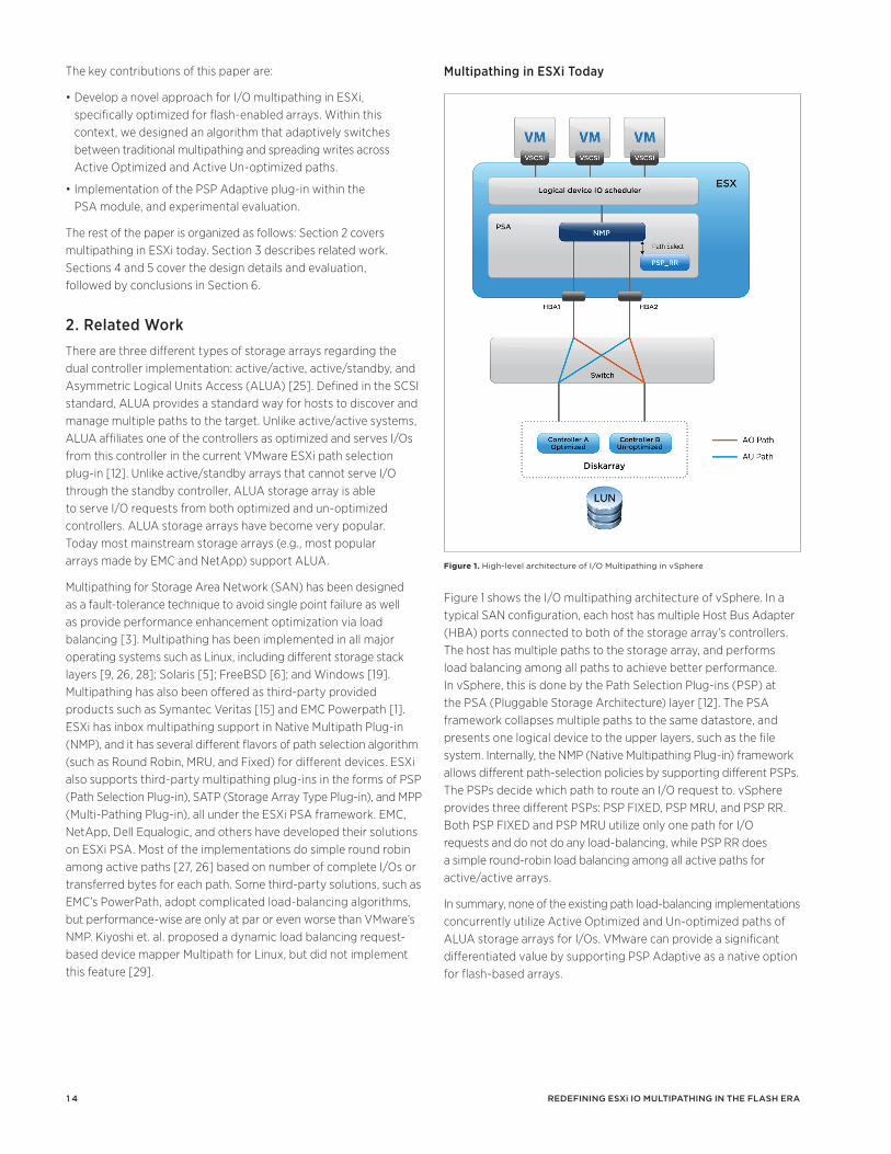
Multipathing in ESXi Today

Figure 1 shows the I/O multipathing architecture of vSphere. In a typical SAN configuration, each host has multiple Host Bus Adapter (HBA) ports connected to both of the storage array’s controllers. The host has multiple paths to the storage array, and performs load balancing among all paths to achieve better performance. In vSphere, this is done by the Path Selection Plug-ins (PSP) at the PSA (Pluggable Storage Architecture) layer [12]. The PSA framework collapses multiple paths to the same datastore, and presents one logical device to the upper layers, such as the file system. Internally, the NMP (Native Multipathing Plug-in) framework allows different path-selection policies by supporting different PSPs. The PSPs decide which path to route an I/O request to. vSphere provides three different PSPs: PSP FIXED, PSP MRU, and PSP RR. Both PSP FIXED and PSP MRU utilize only one path for I/O requests and do not do any load-balancing, while PSP RR does a simple round-robin load balancing among all active paths for active/active arrays.

In summary, none of the existing path load-balancing implementations concurrently utilize Active Optimized and Un-optimized paths of ALUA storage arrays for I/Os. VMware can provide a significant differentiated value by supporting PSP Adaptive as a native option for flash-based arrays.

The key contributions of this paper are:

•DevelopanovelapproachforI/OmultipathinginESXi,specifically optimized for flash-enabled arrays. Within this context, we designed an algorithm that adaptively switches between traditional multipathing and spreading writes across Active Optimized and Active Un-optimized paths.

•ImplementationofthePSPAdaptiveplug-inwithinthe PSA module, and experimental evaluation.

The rest of the paper is organized as follows: Section 2 covers multipathing in ESXi today. Section 3 describes related work. Sections 4 and 5 cover the design details and evaluation, followed by conclusions in Section 6.

2. Related WorkThere are three different types of storage arrays regarding the dual controller implementation: active/active, active/standby, and Asymmetric Logical Units Access (ALUA) [25]. Defined in the SCSI standard, ALUA provides a standard way for hosts to discover and manage multiple paths to the target. Unlike active/active systems, ALUA affiliates one of the controllers as optimized and serves I/Os from this controller in the current VMware ESXi path selection plug-in [12]. Unlike active/standby arrays that cannot serve I/O through the standby controller, ALUA storage array is able to serve I/O requests from both optimized and un-optimized controllers. ALUA storage arrays have become very popular. Today most mainstream storage arrays (e.g., most popular arrays made by EMC and NetApp) support ALUA.

Multipathing for Storage Area Network (SAN) has been designed as a fault-tolerance technique to avoid single point failure as well as provide performance enhancement optimization via load balancing [3]. Multipathing has been implemented in all major operating systems such as Linux, including different storage stack layers [9, 26, 28]; Solaris [5]; FreeBSD [6]; and Windows [19]. Multipathing has also been offered as third-party provided products such as Symantec Veritas [15] and EMC Powerpath [1]. ESXi has inbox multipathing support in Native Multipath Plug-in (NMP), and it has several different flavors of path selection algorithm (such as Round Robin, MRU, and Fixed) for different devices. ESXi also supports third-party multipathing plug-ins in the forms of PSP (Path Selection Plug-in), SATP (Storage Array Type Plug-in), and MPP (Multi-Pathing Plug-in), all under the ESXi PSA framework. EMC, NetApp, Dell Equalogic, and others have developed their solutions on ESXi PSA. Most of the implementations do simple round robin among active paths [27, 26] based on number of complete I/Os or transferred bytes for each path. Some third-party solutions, such as EMC’s PowerPath, adopt complicated load-balancing algorithms, but performance-wise are only at par or even worse than VMware’s NMP. Kiyoshi et. al. proposed a dynamic load balancing request-based device mapper Multipath for Linux, but did not implement this feature [29].

Figure 1. High-level architecture of I/O Multipathing in vSphere


1 5

cases, spreading writes to un-optimized paths will help lower the load on the optimized paths, and thereby boost system performance. Thus in our optimized plug-in, only writes are spread to un-optimized paths.

3.3 Spread Start and Stop TriggersBecause of the asymmetric performance between optimized and un-optimized paths, we should only spread I/O to un-optimized paths when the optimized paths are saturated (i.e., there is I/O contention). Therefore, accurate I/O contention detection is the key. Another factor we need to consider is that the ALUA specification does not specify the implementation details. Therefore different ALUA arrays from different vendors could have different ALUA implementations and hence different behaviors on serving I/O issued on the un-optimized paths. In our experiments, we have found that at least one ALUA array shows unacceptable performance for I/Os issued on the un-optimized paths. We need to take this into account, and design the PSP Adaptive to be able to detect such behavior and stop routing WRITEs to the un-optimized paths if no I/O performance improvement is observed. The following sections describe the implementation details.

3.3.1 I/O Contention DetectionWe apply the same techniques that SIOC (Storage I/O Control) uses today to the PSP Adaptive for I/O contention detection: use I/O latency thresholds. To avoid thrashing, two latency thresholds ta and tb (ta > ta) are used to trigger start and stop of write spread to non-optimized paths. PSP Adaptive keeps monitoring I/O latency

3. Design and ImplementationConsider a highway and a local road, both to the same destination. When the traffic is bounded by a toll plaza at the destination, there is no point to route traffic to the local road. However, if the toll plaza is removed, it starts to make sense to route a part of traffic to the local road during rush hours, because now the contention point has shifted. The same strategy can be applied to the load-balancing strategy for ALUA storage arrays. When the array is the contention point, there is no point in routing I/O requests to the non-optimized paths: the latency is higher, and host-side I/O bandwidth is not the bound. However, when the array with flash is able to serve millions of IOPS, it is no longer the contention point, and host-side I/O pipes could become the contention point during heavy I/O load. It starts to make sense to route a part of the I/O traffic to the un-optimized paths. Although the latency on the un-optimized paths is higher, considering the optimized paths are saturated, using un-optimized paths can still boost aggregated system I/O performance with increased I/O throughput and IOPS. This should only be done during “rush hours,” when the I/O load is heavy and the optimized paths are saturated. A new PSP Adaptive is implemented using this strategy.

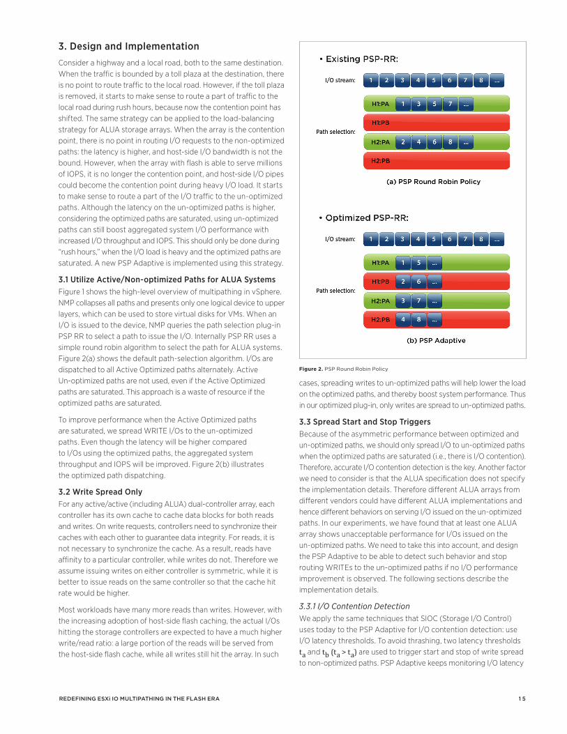
3.1 Utilize Active/Non-optimized Paths for ALUA SystemsFigure 1 shows the high-level overview of multipathing in vSphere. NMP collapses all paths and presents only one logical device to upper layers, which can be used to store virtual disks for VMs. When an I/O is issued to the device, NMP queries the path selection plug-in PSP RR to select a path to issue the I/O. Internally PSP RR uses a simple round robin algorithm to select the path for ALUA systems. Figure 2(a) shows the default path-selection algorithm. I/Os are dispatched to all Active Optimized paths alternately. Active Un-optimized paths are not used, even if the Active Optimized paths are saturated. This approach is a waste of resource if the optimized paths are saturated.

To improve performance when the Active Optimized paths are saturated, we spread WRITE I/Os to the un-optimized paths. Even though the latency will be higher compared to I/Os using the optimized paths, the aggregated system throughput and IOPS will be improved. Figure 2(b) illustrates the optimized path dispatching.

3.2 Write Spread OnlyFor any active/active (including ALUA) dual-controller array, each controller has its own cache to cache data blocks for both reads and writes. On write requests, controllers need to synchronize their caches with each other to guarantee data integrity. For reads, it is not necessary to synchronize the cache. As a result, reads have affinity to a particular controller, while writes do not. Therefore we assume issuing writes on either controller is symmetric, while it is better to issue reads on the same controller so that the cache hit rate would be higher.

Most workloads have many more reads than writes. However, with the increasing adoption of host-side flash caching, the actual I/Os hitting the storage controllers are expected to have a much higher write/read ratio: a large portion of the reads will be served from the host-side flash cache, while all writes still hit the array. In such

Figure 2. PSP Round Robin Policy


1 6

for optimized paths (to). If to exceeds ta, PSP Adaptive starts to trigger write spread. If to falls below tb, PSP Adaptive stops write spread. Like SIOC, the actual values of ta and tb are set by the user, and could differ for different storage arrays.

3.3.2 Max I/O Latency ThresholdAs described earlier, different storage vendor’s ALUA implementations vary. The I/O performance on the un-optimized paths for some ALUA arrays could be very poor. For such arrays, we should not spread I/O to the un-optimized paths. To handle such cases, we introduce a third threshold: max I/O latency tc( tc > ta). Latency higher than this value is unacceptable to the user. PSP Adaptive monitors I/O latency on un-optimized paths (tuo) when write spread is turned on. If PSP Adaptive detects tuo exceeding the value of tc, it concludes that the un-optimized paths should not be used and stops write spread.

A simple on/off switch is also added as a configurable knob for administrators. If a user does not want to use un-optimized paths, an administrator can simply turn the feature off through the esxcli command. PSP Adaptive will behave the same as PSP RR in such cases, without spreading I/O to un-optimized paths.

3.3.3 I/O Performance Improvement DetectionWe want to spread I/O to un-optimized paths only if it improves aggregated system IOPS and/or throughput. PSP Adaptive continues monitoring aggregated IOPS and throughput on all paths to the specific target. Detecting I/O performance improvements is more complicated, however, since system load and I/O patterns (e.g. block size) could change. I/O latency numbers cannot be used to decide if the system performance improves or not for this reason.

To handle this situation, we monitor and compare both IOPS and throughput numbers. When I/O latency on optimized paths exceeds threshold ta, PSP Adaptive saves the IOPS and throughput data as the reference values before it turns on write spread to un-optimized paths. It then periodically checks if the aggregated IOPS and/or throughput improved by comparing them against the reference values. If not improved, it will stop write spread; otherwise, no actions are taken. To avoid noise, at least 10% improvement on either IOPS or throughput is required to conclude that performance is improved.

Overall system performance is considered improved even if only one of the two measures (IOPS and throughput) improves. This is because I/O pattern change should not decrease both values simultaneously. For example, if I/O block sizes go down, aggregated throughput could go down, but IOPS should go up. If system load goes up, both IOPS and throughput should go up with write spread. If both aggregated IOPS and throughput go down, PSP Adaptive concludes that it is because system load is going down.

If system load goes down, the aggregated IOPS and throughput could go down as well and cause PSP Adaptive to stop write spread. This is fine, because less system load means I/O latency will be improved. Unless the I/O latency on optimized paths exceeds ta again, write spread will not be turned on again.

3.3.4 Impact on Other Hosts in the Same ClusterUsually one host utilizing the un-optimized paths could negatively affect other hosts that are connected to the same ALUA storage array. However, as explained in the earlier sections, the greatly boosted I/O performance of new flash-based storage means the

storage array is much less likely to become the contention point—even if multiple hosts are pumping heavy I/O load to the array simultaneously. Thereby the negative impact here is negligible. Our performance benchmark also proves that.

4. Evaluation and AnalysisAll the performance numbers are collected on one ESXi server. The physical machine configuration is listed in Table 1. Iometer running inside Windows VMs is used to generate workload. Since vFlash and VFC were not available at the time the prototype was done, we used Iometer load with 50% random read and 50% random write to simulate the effect of host-side caching which changes the I/O READ/WRITE ratio hitting the array.

CPU 2 Intel Xeon, 8 Cores, 16 Logical CPUs

Memory 96GB DRAM

HBA Dual port 8Gbps HBA

Storage Array ALUA enabled array with 16 LUNs on SSD, each LUN 100MB

FC Switch 8Gbps FC switch

Table 1. Testbed Configuration

Figure 3 and Figure 4 compare the performance of PSP RR and PSP Adaptive when there is I/O contention on the HBA port. By spreading WRITEs to un-optimized paths during I/O contention, PSP Adaptive is able to increase aggregated system IOPS and throughput, at the cost of slightly higher average WRITE latency. The aggregated system throughput improvement also increases with increasing I/O block size.

Overall, the performance evaluation results show that PSP Adaptive can increase system aggregated throughput and IOPS during I/O contention, and is self-adaptive to workload changes.

Figure 3. Throughput: PSP RR vs PSP Adaptive


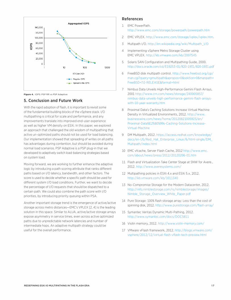
1 7

References1 EMC PowerPath.

http://www.emc.com/storage/powerpath/powerpath.htm

2 EMC VPLEX. http://www.emc.com/storage/vplex/vplex.htm.

3 Multipath I/O. http://en.wikipedia.org/wiki/Multipath_I/O

4 Implementing vSphere Metro Storage Cluster using EMC VPLEX. http://kb.vmware.com/kb/2007545

5 Solaris SAN Configuration and Multipathing Guide, 2000. http://docs.oracle.com/cd/E19253-01/820-1931/820-1931.pdf

6 FreeBSD disk multipath control. http://www.freebsd.org/cgi/man.cgi?query=gmultipath&apropos=0&sektion=0&manpath=FreeBSD+7.0-RELEASE&format=html

7 Nimbus Data Unveils High-Performance Gemini Flash Arrays, 2001 http://www.crn.com/news/storage/240005857/nimbus-data-unveils-high-performance-gemini-flash-arrays-with-10-year-warranty.htm

8 Proximal Data’s Caching Solutions Increase Virtual Machine Density in Virtualized Environments, 2012. http://www.businesswire.com/news/home/20120821005923/en/Proximal-Data%E2%80%99s-Caching-Solutions-Increase-Virtual-Machine

9 DM Multipath, 2012. https://access.redhat.com/knowledge/docs/en-US/Red_Hat_Enterprise_Linux/6/html-single/DM_Multipath/index.html

10 EMC vfcache, Server Flash Cache, 2012 http://www.emc.com/about/news/press/2012/20120206-01.htm

11 Flash and Virtualization Take Center Stage at SNW for Avere., 2012. http://www.averesystems.com/

12 Multipathing policies in ESXi 4.x and ESXi 5.x, 2012. http://kb.vmware.com/kb/1011340

13 No-Compromise Storage for the Modern Datacenter, 2012, http://info.nimblestorage.com/rs/nimblestorage/images/Nimble_Storage_Overview_White_Paper.pdf

14 Pure Storage: 100% flash storage array: Less than the cost of spinning disk, 2012. http://www.purestorage.com/flash-array/

15 Symantec Veritas Dynamic Multi-Pathing, 2012. http://www.symantec.com/docs/DOC5811

16 Violin memory, 2012. http://www.violin-memory.com/

17 VMware vFlash framework, 2012. http://blogs.vmware.com/vsphere/2012/12/virtual-flash-vflash-tech-preview.html

5. Conclusion and Future WorkWith the rapid adoption of flash, it is important to revisit some of the fundamental building blocks of the vSphere stack. I/O multipathing is critical for scale and performance, and any improvements translate into improved end-user experience as well as higher VM density on ESXi. In this paper, we explored an approach that challenged the old wisdom of multipathing that active un-optimized paths should not be used for load balancing. Our implementation showed that spreading of writes on all paths has advantages during contention, but should be avoided during normal load scenarios. PSP Adaptive is a PSP plug-in that we developed to adaptively switch load-balancing strategies based on system load.

Moving forward, we are working to further enhance the adaptive logic by introducing a path scoring attribute that ranks different paths based on I/O latency, bandwidth, and other factors. The score is used to decide whether a specific path should be used for different system I/O load conditions. Further, we want to decide the percentage of I/O requests that should be dispatched to a certain path. We could also combine the path score with I/O priorities, by introducing priority queuing within PSA.

Another important storage trend is the emergence of active/active storage across metro distances—EMC’s VPLEX [2, 4] is the leading solution in this space. Similar to ALUA, active/active storage arrays expose asymmetry in service times, even across active optimized paths due to unpredictable network latencies and number of intermediate hops. An adaptive multipath strategy could be useful for the overall performance.

Figure 4. IOPS: PSP RR vs PSP Adaptive


http://www.freebsd.org/cgi/man.cgi?query=gmultipath&apropos=0&sektion=0&manpath=FreeBSD+7.0-RELEASE&format=html



http://www.crn.com/news/storage/240005857/nimbus-data-unveils-high-performance-gemini-flash-arrays-with-10-year-warranty.htm



http://www.businesswire.com/news/home/20120821005923/en/Proximal-Data%E2%80%99s-Caching-Solutions-Increase-Virtual-Machine




https://access.redhat.com/knowledge/docs/en-US/Red_Hat_Enterprise_Linux/6/html-single/DM_Multipath/index.html



http://www.emc.com/about/news/press/2012/20120206-01.htm

http://www.emc.com/about/news/press/2012/20120206-01.htm

http://info.nimblestorage.com/rs/nimblestorage/images/Nimble_Storage_Overview_White_Paper.pdf

http://info.nimblestorage.com/rs/nimblestorage/images/Nimble_Storage_Overview_White_Paper.pdf

http://blogs.vmware.com/vsphere/2012/12/virtual-flash-vflash-tech-preview.html

http://blogs.vmware.com/vsphere/2012/12/virtual-flash-vflash-tech-preview.html

1 8

24 BYAN, S., LENTINI, J., MADAN, A., AND PABON, L. Mercury: Host-side Flash Caching for the Data Center. InMSST (2012), IEEE, pp. 1–12.

25 EMC ALUA System. http://www.emc.com/collateral/hardware/white-papers/h2890-emc-clariion-asymm-active-wp.pdf

26 KIYOSHI UEDA, JUNICHI NOMURA, M. C. Request-based Device-mapper multipath and Dynamic load balancing. In Proceedings of the Linux Symposium (2007)

27 LUO, J., SHU, J.-W., AND XUE, W. Design and Implementation of an Efficient Multipath for a SAN Environment. In Proceedings of the 2005 international conference on Parallel and Distributed Processing and Applications (Berlin, Heidelberg, 2005), ISPA’05, Springer-Verlag, pp. 101–110.

28 MICHAEL ANDERSON, P. M. SCSI Mid-Level Multipath. In Proceedings of the Linux Symposium (2003).

29 UEDA, K. Request-based dm-multipath, 2008. http://lwn.net/Articles/274292/.

18 Who is WHIPTAIL?, 2012, http://whiptail.com/papers/who-is-whiptail/

19 Windows Multipath I/O, 2012. http://technet.microsoft.com/en-us/library/cc725907.aspx.

20 XtremIO, 2012. http://www.xtremio.com/

21 NetApp Quietly Absorbs CacheIQ, Nov, 2012, http://www.networkcomputing.com/storage-networkingmanagement/netapp-quietly-absorbs-cacheiq/240142457

22 SolidFire Reveals New Arrays for White Hot Flash Market, Nov, 2012 http://siliconangle.com/blog/2012/11/13/solidfire-reveals-new-arrays-for-white-hot-flash-market//

23 Gridiron Intros New Flash Storage Appliance, Hybrid Flash Array, Oct, 2012. http://www.crn.com/news/storage/240008223/gridiron-introsnew-flash-storage-appliance-hybrid-flash-array.htm


http://www.emc.com/collateral/hardware/white-papers/h2890-emc-clariion-asymm-active-wp.pdf

http://www.emc.com/collateral/hardware/white-papers/h2890-emc-clariion-asymm-active-wp.pdf

http://www.networkcomputing.com/storage-networkingmanagement/netapp-quietly-absorbs-cacheiq/240142457



http://siliconangle.com/blog/2012/11/13/solidfire-reveals-new-arrays-for-white-hot-flash-market//

http://siliconangle.com/blog/2012/11/13/solidfire-reveals-new-arrays-for-white-hot-flash-market//

http://www.crn.com/news/storage/240008223/gridiron-introsnew-flash-storage-appliance-hybrid-flash-array.htm



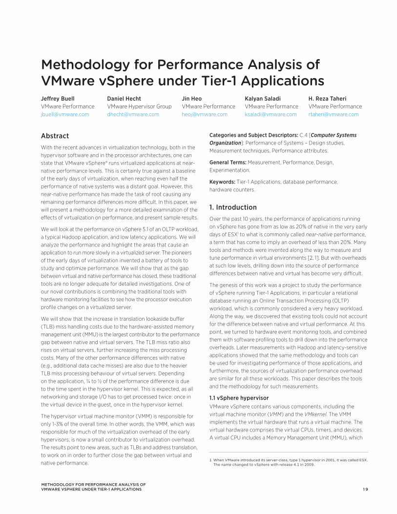
1 9

Categories and Subject Descriptors: C.4 [Computer Systems Organization]: Performance of Systems – Design studies, Measurement techniques, Performance attributes.

General Terms: Measurement, Performance, Design, Experimentation.

Keywords: Tier-1 Applications, database performance, hardware counters.

1. IntroductionOver the past 10 years, the performance of applications running on vSphere has gone from as low as 20% of native in the very early days of ESX1 to what is commonly called near-native performance, a term that has come to imply an overhead of less than 20%. Many tools and methods were invented along the way to measure and tune performance in virtual environments [2, 1]. But with overheads at such low levels, drilling down into the source of performance differences between native and virtual has become very difficult.

The genesis of this work was a project to study the performance of vSphere running Tier-1 Applications, in particular a relational database running an Online Transaction Processing (OLTP) workload, which is commonly considered a very heavy workload. Along the way, we discovered that existing tools could not account for the difference between native and virtual performance. At this point, we turned to hardware event monitoring tools, and combined them with software profiling tools to drill down into the performance overheads. Later measurements with Hadoop and latency-sensitive applications showed that the same methodology and tools can be used for investigating performance of those applications, and furthermore, the sources of virtualization performance overhead are similar for all these workloads. This paper describes the tools and the methodology for such measurements.

1.1 vSphere hypervisorVMware vSphere contains various components, including the virtual machine monitor (VMM) and the VMkernel. The VMM implements the virtual hardware that runs a virtual machine. The virtual hardware comprises the virtual CPUs, timers, and devices. A virtual CPU includes a Memory Management Unit (MMU), which

AbstractWith the recent advances in virtualization technology, both in the hypervisor software and in the processor architectures, one can state that VMware vSphere® runs virtualized applications at near-native performance levels. This is certainly true against a baseline of the early days of virtualization, when reaching even half the performance of native systems was a distant goal. However, this near-native performance has made the task of root causing any remaining performance differences more difficult. In this paper, we will present a methodology for a more detailed examination of the effects of virtualization on performance, and present sample results.

We will look at the performance on vSphere 5.1 of an OLTP workload, a typical Hadoop application, and low latency applications. We will analyze the performance and highlight the areas that cause an application to run more slowly in a virtualized server. The pioneers of the early days of virtualization invented a battery of tools to study and optimize performance. We will show that as the gap between virtual and native performance has closed, these traditional tools are no longer adequate for detailed investigations. One of our novel contributions is combining the traditional tools with hardware monitoring facilities to see how the processor execution profile changes on a virtualized server.

We will show that the increase in translation lookaside buffer (TLB) miss handling costs due to the hardware-assisted memory management unit (MMU) is the largest contributor to the performance gap between native and virtual servers. The TLB miss ratio also rises on virtual servers, further increasing the miss processing costs. Many of the other performance differences with native (e.g., additional data cache misses) are also due to the heavier TLB miss processing behaviour of virtual servers. Depending on the application, ¼ to ½ of the performance difference is due to the time spent in the hypervisor kernel. This is expected, as all networking and storage I/O has to get processed twice: once in the virtual device in the guest, once in the hypervisor kernel.

The hypervisor virtual machine monitor (VMM) is responsible for only 1-3% of the overall time. In other words, the VMM, which was responsible for much of the virtualization overhead of the early hypervisors, is now a small contributor to virtualization overhead. The results point to new areas, such as TLBs and address translation, to work on in order to further close the gap between virtual and native performance.

Methodology for performance analysis of VMware vSphere under tier-1 applicationsJeffrey Buell Daniel Hecht Jin Heo Kalyan Saladi H. Reza Taheri VMware Performance VMware Hypervisor Group VMware Performance VMware Performance VMware Performance [email protected] [email protected] [email protected] [email protected] [email protected]

Methodology for perforMance analySiS of vMware vSphere under tier-1 applicationS

1 When VMware introduced its server-class, type 1 hypervisor in 2001, it was called ESX. The name changed to vSphere with release 4.1 in 2009.

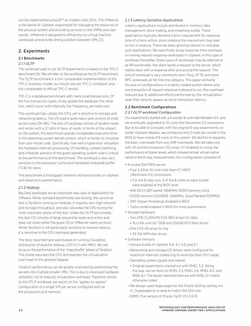
2 0

2.1.3 Latency-Sensitive ApplicationsLatency applications include distributed in-memory data management, stock trading, and streaming media. These applications typically demand a strict requirement for response time of a trans-action, since violating the requirement may lead to loss in revenue. There has been growing interest to virtualize such applications. We specifically study response-time overhead in running request-response workloads in vSphere. In this type of workload (hereafter, these types of workloads may be referred to as RR workloads), the client sends a request to the server, which replies back with a response after processing the request. This kind of workload is very commonly seen: Ping, HTTP, and most RPC workloads all fall into the category. This paper primarily focuses on configurations in a lightly loaded system where only one transaction of request-response is allowed to run. Any overhead induced due to additional efforts performed by the virtualization layer then directly appear as extra transaction latency.

2.2 Benchmark Configurations2.2.1 OLTP workload ConfigurationOur experiments started with a 4-socket, 8-core Intel Nehalem-EX, and we eventually upgraded to 10-core Intel Westmere-EX processors. But to be able to compare with the original 8-way experiments on earlier vSphere releases, we configured only 2 cores per socket in the BIOS to have a total of 8 cores on the system. We did this to separate the basic overheads from any SMP overheads. We did take runs with 32 and 64 processors (32 cores, HT enabled) to study the performance at higher levels, which showed similar virtual-native ratios to the 8-way measurements. Our configuration consisted of:

•4-socketDellR910server

Four 2.4GHz 10-core Intel Xeon E7-4870 –(Westmere-EX) processors

For the 8-way runs, 2 of the 8 cores on each socket •were enabled at the BIOS level

4X6.4GT/s QPI speed; 1066MHz DDR3 memory clock –

512GB memory (32x16GB, 1066MHz, Quad Ranked RDIMMs) –

SMT (hyper-threading) disabled in BIOS –

Turbo mode enabled in BIOS for most experiments –

•StorageHardware

Two EMC CLARiiON CX4-960 arrays for data –

16 LUNs over 62 73GB and 200GB EFD flash drives•

One CX3-40 array for log –

30 15K RPM disk drives•

•SoftwareVersions

Various builds of vSphere 4.0, 4.1, 5.0, and 5.1 –

Networking and storage I/O drivers were configured for –maximum interrupt coalescing to minimize their CPU usage

Operating system (guest and native): –

Original experiments started out with RHEL 5.2. Along •the way, we ran tests on RHEL 5.3, RHEL 5.6, RHEL 6.0, and RHEL 6.1. The results reported here are with RHEL 6.1 unless otherwise noted

We always used large pages for the Oracle SGA by setting vm. –nr_hugepages to a value to match the SGA size

DBMS Trial version of Ora – cle 11g R1 (11.1.0.6.0)

can be implemented using EPT on modern Intel CPUs. The VMkernel is the kernel of vSphere, responsible for managing the resources of the physical system and providing services to the VMMs and user worlds. VMkernel is designed to efficiently run virtual machine workloads and provide strong isolation between VMs [2].

2. Experiments2.1 Benchmarks2.1.1 OLTPThe workload used in our OLTP experiments is based on the TPC-C benchmark [9]. We will refer to this workload as the OLTP benchmark. The OLTP benchmark is a non-comparable implementation of the TPC-C business model; our results are not TPC-C compliant, and not comparable to official TPC-C results.

TPC-C is a database benchmark with many small transactions. Of the five transaction types, three update the database; the other two, which occur with relatively low frequency, are read-only.

This workload fully utilizes the CPU, yet is sensitive to storage and networking latency. The I/O load is quite heavy and consists of small access sizes (2K-16K). The disk I/O accesses consist of random reads and writes with a 2:1 ratio in favor of reads. In terms of the impact on the system, this benchmark spends considerable execution time in the operating system kernel context, which is harder to virtualize than user-mode code. Specifically, how well a hypervisor virtualizes the hardware interrupt processing, I/O handling, context switching, and scheduler portions of the guest operating system code is critical to the performance of this benchmark. The workload is also very sensitive to the processor cache and translation lookaside buffer (TLB) hit ratios.

This benchmark is the biggest hammer we have to beat on vSphere and observe its performance.

2.1.2 HadoopBig Data workloads are an important new class of applications for VMware. While standard benchmarks are lacking, the canonical test is TeraSort running on Hadoop. It requires very high network and storage throughput, and also saturates the CPU during the most important phase of the test. Unlike the OLTP benchmark, the disk I/O consists of large sequential reads and writes and does not stress either the guest OS or VMkernel nearly as much. While TeraSort is not particularly sensitive to network latency, it is sensitive to the CPU overhead generated.

The tests reported here were based on running Cloudera’s distribution of Apache Hadoop, CDH 4.1.1 with MRv1. We will focus on the performance of the “map/shuffle” phase of TeraSort. This phase saturates the CPU and exposes the virtualization over-head to the greatest degree.

TeraSort performance can be greatly improved by partitioning the servers into multiple smaller VMs. This is due to improved hardware utilization, not to reduced virtualization overhead. Therefore, similar to the OTLP workload, we report on the “apples-to-apples” configuration of a single VM per server configured with all the processors and memory.


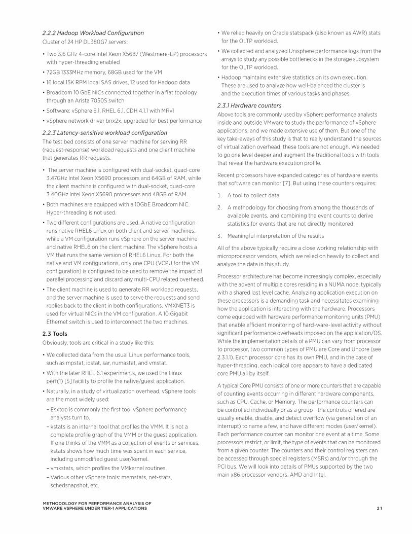
2 1

•WereliedheavilyonOraclestatspack(alsoknownasAWR)statsfor the OLTP workload.

•WecollectedandanalyzedUnisphereperformancelogsfromthearrays to study any possible bottlenecks in the storage subsystem for the OLTP workload.

•Hadoopmaintainsextensivestatisticsonitsownexecution.These are used to analyze how well-balanced the cluster is and the execution times of various tasks and phases.

2.3.1 Hardware countersAbove tools are commonly used by vSphere performance analysts inside and outside VMware to study the performance of vSphere applications, and we made extensive use of them. But one of the key take-aways of this study is that to really understand the sources of virtualization overhead, these tools are not enough. We needed to go one level deeper and augment the traditional tools with tools that reveal the hardware execution profile.

Recent processors have expanded categories of hardware events that software can monitor [7]. But using these counters requires:

1. A tool to collect data

2. A methodology for choosing from among the thousands of available events, and combining the event counts to derive statistics for events that are not directly monitored

3. Meaningful interpretation of the results

All of the above typically require a close working relationship with microprocessor vendors, which we relied on heavily to collect and analyze the data in this study.

Processor architecture has become increasingly complex, especially with the advent of multiple cores residing in a NUMA node, typically with a shared last level cache. Analyzing application execution on these processors is a demanding task and necessitates examining how the application is interacting with the hardware. Processors come equipped with hardware performance monitoring units (PMU) that enable efficient monitoring of hard-ware-level activity without significant performance overheads imposed on the application/OS. While the implementation details of a PMU can vary from processor to processor, two common types of PMU are Core and Uncore (see 2.3.1.1). Each processor core has its own PMU, and in the case of hyper-threading, each logical core appears to have a dedicated core PMU all by itself.

A typical Core PMU consists of one or more counters that are capable of counting events occurring in different hardware components, such as CPU, Cache, or Memory. The performance counters can be controlled individually or as a group—the controls offered are usually enable, disable, and detect overflow (via generation of an interrupt) to name a few, and have different modes (user/kernel). Each performance counter can monitor one event at a time. Some processors restrict, or limit, the type of events that can be monitored from a given counter. The counters and their control registers can be accessed through special registers (MSRs) and/or through the PCI bus. We will look into details of PMUs supported by the two main x86 processor vendors, AMD and Intel.

2.2.2 Hadoop Workload ConfigurationCluster of 24 HP DL380G7 servers:

•Two3.6GHz4-coreIntelXeonX5687(Westmere-EP)processorswith hyper-threading enabled

•72GB1333MHzmemory,68GBusedfortheVM

•16local15KRPMlocalSASdrives,12usedforHadoopdata

•Broadcom10GbENICsconnectedtogetherinaflattopologythrough an Arista 7050S switch

•Software:vSphere5.1,RHEL6.1,CDH4.1.1withMRv1

•vSpherenetworkdriverbnx2x,upgradedforbestperformance

2.2.3 Latency-sensitive workload configurationThe test bed consists of one server machine for serving RR (request-response) workload requests and one client machine that generates RR requests.

•Theservermachineisconfiguredwithdual-socket,quad-core3.47GHz Intel Xeon X5690 processors and 64GB of RAM, while the client machine is configured with dual-socket, quad-core 3.40GHz Intel Xeon X5690 processors and 48GB of RAM.

•Bothmachinesareequippedwitha10GbEBroadcomNIC.Hyper-threading is not used.

•Twodifferentconfigurationsareused.Anativeconfigurationruns native RHEL6 Linux on both client and server machines, while a VM configuration runs vSphere on the server machine and native RHEL6 on the client machine. The vSphere hosts a VM that runs the same version of RHEL6 Linux. For both the native and VM configurations, only one CPU (VCPU for the VM configuration) is configured to be used to remove the impact of parallel processing and discard any multi-CPU related overhead.

•TheclientmachineisusedtogenerateRRworkloadrequests,and the server machine is used to serve the requests and send replies back to the client in both configurations. VMXNET3 is used for virtual NICs in the VM configuration. A 10 Gigabit Ethernet switch is used to interconnect the two machines.

2.3 ToolsObviously, tools are critical in a study like this:

•WecollecteddatafromtheusualLinuxperformancetools, such as mpstat, iostat, sar, numastat, and vmstat.

•WiththelaterRHEL6.1experiments,weusedtheLinux perf(1) [5] facility to profile the native/guest application.

•Naturally,inastudyofvirtualizationoverhead,vSpheretools are the most widely used:

Esxtop is commonly the first tool vSphere performance –analysts turn to.

kstats is an internal tool that profiles the VMM. It is not a –complete profile graph of the VMM or the guest application. If one thinks of the VMM as a collection of events or services, kstats shows how much time was spent in each service, including unmodified guest user/kernel.

vmkstats, which profiles the VMkernel routines. –

Various other vSphere tools: memstats, net-stats, –schedsnapshot, etc.


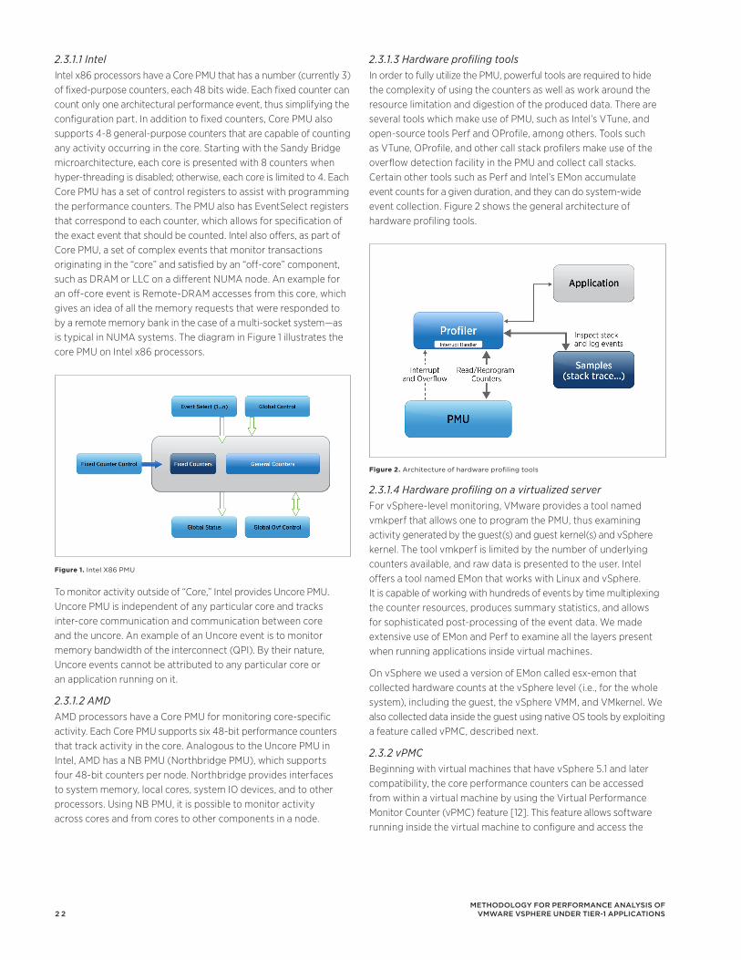
2 2

2.3.1.3 Hardware profiling toolsIn order to fully utilize the PMU, powerful tools are required to hide the complexity of using the counters as well as work around the resource limitation and digestion of the produced data. There are several tools which make use of PMU, such as Intel’s VTune, and open-source tools Perf and OProfile, among others. Tools such as VTune, OProfile, and other call stack profilers make use of the overflow detection facility in the PMU and collect call stacks. Certain other tools such as Perf and Intel’s EMon accumulate event counts for a given duration, and they can do system-wide event collection. Figure 2 shows the general architecture of hardware profiling tools.

2.3.1.4 Hardware profiling on a virtualized serverFor vSphere-level monitoring, VMware provides a tool named vmkperf that allows one to program the PMU, thus examining activity generated by the guest(s) and guest kernel(s) and vSphere kernel. The tool vmkperf is limited by the number of underlying counters available, and raw data is presented to the user. Intel offers a tool named EMon that works with Linux and vSphere. It is capable of working with hundreds of events by time multiplexing the counter resources, produces summary statistics, and allows for sophisticated post-processing of the event data. We made extensive use of EMon and Perf to examine all the layers present when running applications inside virtual machines.

On vSphere we used a version of EMon called esx-emon that collected hardware counts at the vSphere level (i.e., for the whole system), including the guest, the vSphere VMM, and VMkernel. We also collected data inside the guest using native OS tools by exploiting a feature called vPMC, described next.

2.3.2 vPMCBeginning with virtual machines that have vSphere 5.1 and later compatibility, the core performance counters can be accessed from within a virtual machine by using the Virtual Performance Monitor Counter (vPMC) feature [12]. This feature allows software running inside the virtual machine to configure and access the

2.3.1.1 IntelIntel x86 processors have a Core PMU that has a number (currently 3) of fixed-purpose counters, each 48 bits wide. Each fixed counter can count only one architectural performance event, thus simplifying the configuration part. In addition to fixed counters, Core PMU also supports 4-8 general-purpose counters that are capable of counting any activity occurring in the core. Starting with the Sandy Bridge microarchitecture, each core is presented with 8 counters when hyper-threading is disabled; otherwise, each core is limited to 4. Each Core PMU has a set of control registers to assist with programming the performance counters. The PMU also has EventSelect registers that correspond to each counter, which allows for specification of the exact event that should be counted. Intel also offers, as part of Core PMU, a set of complex events that monitor transactions originating in the “core” and satisfied by an “off-core” component, such as DRAM or LLC on a different NUMA node. An example for an off-core event is Remote-DRAM accesses from this core, which gives an idea of all the memory requests that were responded to by a remote memory bank in the case of a multi-socket system—as is typical in NUMA systems. The diagram in Figure 1 illustrates the core PMU on Intel x86 processors.

To monitor activity outside of “Core,” Intel provides Uncore PMU. Uncore PMU is independent of any particular core and tracks inter-core communication and communication between core and the uncore. An example of an Uncore event is to monitor memory bandwidth of the interconnect (QPI). By their nature, Uncore events cannot be attributed to any particular core or an application running on it.

2.3.1.2 AMDAMD processors have a Core PMU for monitoring core-specific activity. Each Core PMU supports six 48-bit performance counters that track activity in the core. Analogous to the Uncore PMU in Intel, AMD has a NB PMU (Northbridge PMU), which supports four 48-bit counters per node. Northbridge provides interfaces to system memory, local cores, system IO devices, and to other processors. Using NB PMU, it is possible to monitor activity across cores and from cores to other components in a node.


Figure 1. Intel X86 PMU

Figure 2. Architecture of hardware profiling tools

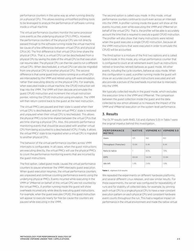
2 3

performance counters in the same way as when running directly on a physical CPU. This allows existing unmodified profiling tools to be leveraged to analyze the performance of software running inside a virtual machine.

The virtual performance counters monitor the same processor core events as the underlying physical CPU’s PMCs. However, the performance counters of the physical CPU are not directly passed through to the software running inside the virtual machine be-cause of a few differences between virtual CPUs and physical CPUs [4]. The first difference is that virtual CPUs time-share the physical CPUs. That is, a virtual CPU can be descheduled from a physical CPU by saving the state of the virtual CPU so that execution can resume later. The physical CPU can then be used to run a different virtual CPU. When descheduled, a virtual CPU can also be migrated from one physical CPU to another physical CPU. The second difference is that some guest instructions running on a virtual CPU are intercepted by the VMM and retired using soft-ware emulation, rather than executing directly on the physical CPU. For example, when executed inside a virtual machine, the CPUID instruction will trap into the VMM. The VMM will then decode and emulate the guest CPUID instruction and increment the virtual instruction pointer, retiring the CPUID instruction using emulation. The VMM will then return control back to the guest at the next instruction.

The virtual PMCs are paused and their state is saved when their virtual CPU is descheduled, and the virtual PMCs’ state is restored and unpaused when their virtual CPU is rescheduled. This allows the physical PMCs to be time-shared between the virtual CPUs that are time-sharing a physical CPU. Also, this prevents performance monitoring events that should be associated with another virtual CPU from being accounted to a descheduled VCPU. Finally, it allows the virtual PMCs’ state to be migrated when a virtual CPU is migrated to another physical CPU.

The behavior of the virtual performance counters across VMM intercepts is configurable. In all cases, when the guest instructions are executing directly, the virtual PMCs will use the physical PMCs to count the performance monitoring events that are incurred by the guest instructions.

The first option, called guest mode, causes the virtual performance counters to pause whenever the VMM intercepts guest execution. When guest execution resumes, the virtual performance counters are unpaused and continue counting performance events using the underlying physical PMCs. Events incurred while executing in the VMM or VMkernel on behalf of this virtual CPU are not counted by the virtual PMCs. A profiler running inside the guest will show overheads incurred only while directly executing guest instructions. For example, when the guest executes CPUID, this guest instruction will appear to execute nearly for free be-cause the counters are paused while executing in the VMM.

The second option is called vcpu mode. In this mode, virtual performance counters continue to count even across an intercept into the VMM. A profiler running inside the guest will show all the events incurred, even while executing the VMM and VMkernel on behalf of the virtual CPU. That is, the profiler will be able to accurately account the time that is required to execute a guest CPUID instruction. The profiler will also show that many instructions were retired when the guest executes a single CPUID instruction, because all the VMM instructions that were executed in order to emulate the CPUID will be accounted.

The third option is a mixture of the first two options and is called hybrid mode. In this mode, any virtual performance counter that is configured to count an at-retirement event (such as instructions retired or branches retired) behaves as guest mode. All other events, including the cycle counters, behave as vcpu mode. When this configuration is used, a profiler running inside the guest will show an accurate count of guest instructions executed and will also provide a picture of the overheads incurred due to intercepts into the VMM.

We typically collected results in the guest mode, which excludes the execution time in the VMM and VMkernel. The comparison between the guest collection inside the guest and the data collected by esx-emon allowed us to measure the impact of the VMM and VMkernel execution on the system level performance.

3. ResultsThe OLTP results (with RHEL 5.6 and vSphere 5.0) in Table 1 were the original impetus behind this investigation.

pErFOrMancE MEtric

natiVE VSphErE 4.1 VSphErE 5.0

Users 125 160 160

Throughput (Trans/sec) 10.6K 8.4K 8.4K

Ratio to native 1 80% 79%

IOPS 68.6K 54.0K 53.8K

Idle left 1.4% 2.6% 1.8%

Table 1. vSphere 5.0 results

We repeated the experiments on different hardware platforms, and several different Linux releases, and saw similar results. For these experiments, the server was configured for repeatability of runs and for stability of collected data, for example, by pinning each virtual CPU to a single physical CPU to have a near-constant execution pattern on each physical CPU and consistent hardware event counts throughout the run. This had a negative impact on performance in the virtual environment and made the native-virtual


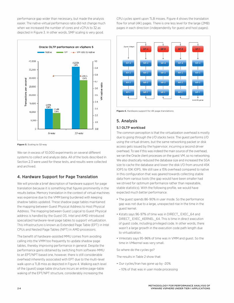
2 4

performance gap wider than necessary, but made the analysis easier. The native-virtual performance ratio did not change much when we increased the number of cores and vCPUs to 32 as depicted in Figure 3. In other words, SMP scaling is very good.

We ran in excess of 10,000 experiments on several different systems to collect and analyze data. All of the tools described in Section 2.3 were used for these tests, and results were collected and archived.

4. Hardware Support for Page TranslationWe will provide a brief description of hardware support for page translation because it is something that figures prominently in the results below. Memory translation in the context of virtual machines was expensive due to the VMM being burdened with keeping shadow tables updated. These shadow page tables maintained the mapping between Guest Physical Address to Host Physical Address. The mapping between Guest Logical to Guest Physical address is handled by the Guest OS. Intel and AMD introduced specialized hardware-level page tables to support virtualization. This infrastructure is known as Extended Page Table (EPT) in Intel CPUs and Nested Page Tables (NPT) in AMD processors.

The benefit of hardware-assisted MMU comes from avoiding calling into the VMM too frequently to update shadow page tables, thereby improving performance in general. Despite the performance gains obtained by switching from software-MMU to an EPT/NPT based one, however, there is still considerable overhead inherently associated with EPT due to the multi-level walk upon a TLB miss as depicted in Figure 4. Walking each level of the (guest) page table structure incurs an entire page-table waking of the EPT/NPT structure, considerably increasing the

CPU cycles spent upon TLB misses. Figure 4 shows the translation flow for small (4K) pages. There is one less level for the large (2MB) pages in each direction (independently for guest and host pages).

5. Analysis5.1 OLTP workloadThe common perception is that the virtualization overhead is mostly due to going through the I/O stacks twice. The guest performs I/O using the virtual drivers, but the same networking packet or disk access gets issued by the hypervisor, incurring a second driver overhead. To see if this was indeed the main source of the overhead, we ran the Oracle client processes on the guest VM, so no networking. We also drastically reduced the database size and increased the SGA size to cache the database and lower the disk I/O from around 45K IOPS to 10K IOPS. We still saw a 15% overhead compared to native in this configuration that was geared towards collecting stable data from various tools (the gap would have been smaller had we strived for optimum performance rather than repeatable, stable statistics). With the following profile, we would have expected much better performance.

•Theguestspends86-90%inusermode.Sotheperformance gap was not due to a large, unexpected rise in the time in the guest kernel.

•Kstatssays96-97%oftimewasinDIRECT_EXEC_64andDIRECT_ EXEC_KERNEL_64. This is time in direct execution of guest code, including privileged code. In other words, there wasn’t a large growth in the execution code path length due to virtualization.

•Vmkstatssays95-96%oftimewasinVMMandguest.Sothetime in VMkernel was very small.

So where do the cycles go?

The results in Table 2 show that:

•Ourcycles/tranhasgoneupby~20%

10% of that was in user mode processing –


Figure 3. Scaling to 32-way

Figure 4. Hardware support for 4K page translations

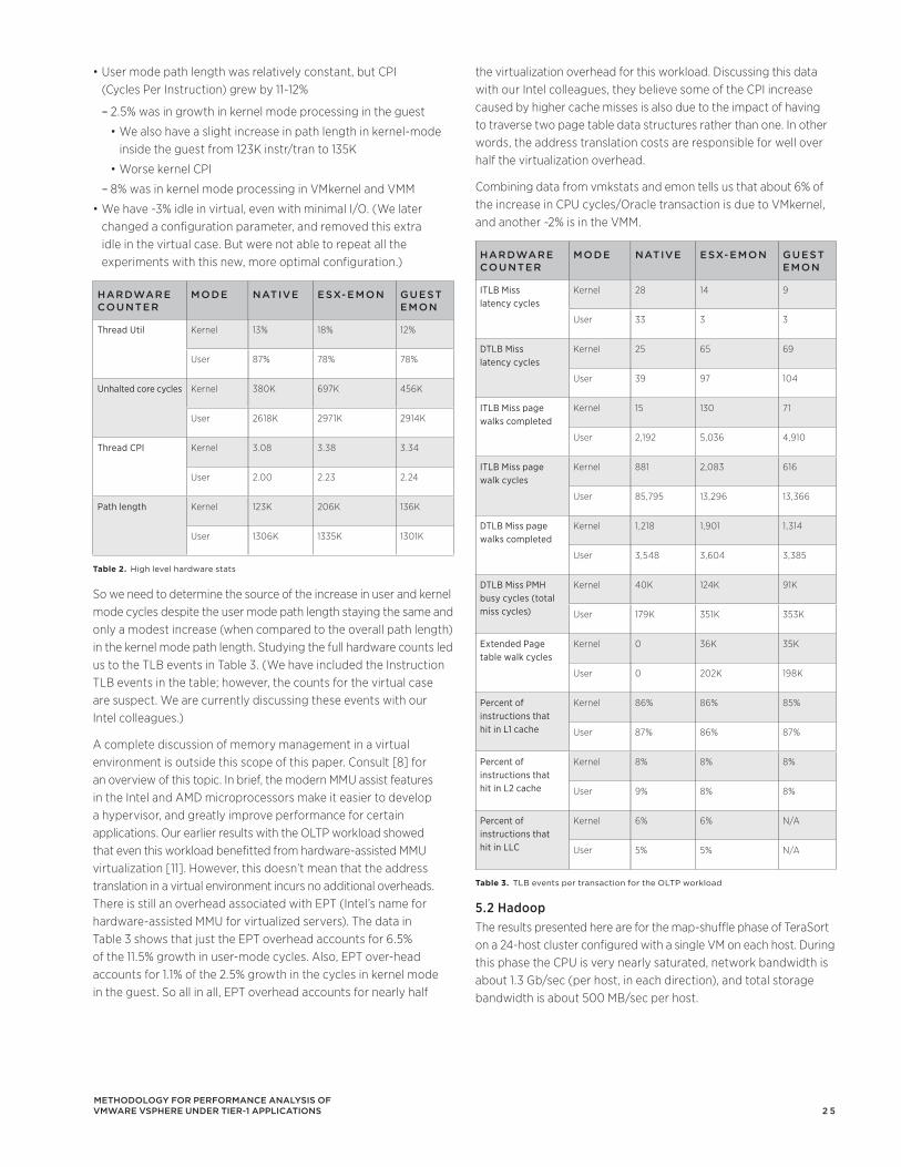
2 5

the virtualization overhead for this workload. Discussing this data with our Intel colleagues, they believe some of the CPI increase caused by higher cache misses is also due to the impact of having to traverse two page table data structures rather than one. In other words, the address translation costs are responsible for well over half the virtualization overhead.

Combining data from vmkstats and emon tells us that about 6% of the increase in CPU cycles/Oracle transaction is due to VMkernel, andanother~2%isintheVMM.

hardwarE cOuntEr

MOdE natiVE ESX-EMOn GuESt EMOn

ITLB Miss latency cycles

Kernel 28 14 9

User 33 3 3

DTLB Miss latency cycles

Kernel 25 65 69

User 39 97 104

ITLB Miss page walks completed

Kernel 15 130 71

User 2,192 5,036 4,910

ITLB Miss page walk cycles

Kernel 881 2,083 616

User 85,795 13,296 13,366

DTLB Miss page walks completed

Kernel 1,218 1,901 1,314

User 3,548 3,604 3,385

DTLB Miss PMH busy cycles (total miss cycles)

Kernel 40K 124K 91K

User 179K 351K 353K

Extended Page table walk cycles

Kernel 0 36K 35K

User 0 202K 198K

Percent of instructions that hit in L1 cache

Kernel 86% 86% 85%

User 87% 86% 87%


Kernel 8% 8% 8%

User 9% 8% 8%

Percent of instructions that hit in LLC

Kernel 6% 6% N/A

User 5% 5% N/A

Table 3. TLB events per transaction for the OLTP workload

5.2 HadoopThe results presented here are for the map-shuffle phase of TeraSort on a 24-host cluster configured with a single VM on each host. During this phase the CPU is very nearly saturated, network bandwidth is about 1.3 Gb/sec (per host, in each direction), and total storage bandwidth is about 500 MB/sec per host.

•Usermodepathlengthwasrelativelyconstant,butCPI (Cycles Per Instruction) grew by 11-12%

2.5% was in growth in kernel mode processing in the guest –

We also have a slight increase in path length in kernel-mode •inside the guest from 123K instr/tran to 135K

Worse kernel CPI•

8% was in kernel mode processing in VMkernel and VMM –

•Wehave~3%idleinvirtual,evenwithminimalI/O.(Welaterchanged a configuration parameter, and removed this extra idle in the virtual case. But were not able to repeat all the experiments with this new, more optimal configuration.)

hardwarE cOuntEr


Thread Util Kernel 13% 18% 12%

User 87% 78% 78%

Unhalted core cycles Kernel 380K 697K 456K

User 2618K 2971K 2914K

Thread CPI Kernel 3.08 3.38 3.34

User 2.00 2.23 2.24

Path length Kernel 123K 206K 136K

User 1306K 1335K 1301K

Table 2. High level hardware stats

So we need to determine the source of the increase in user and kernel mode cycles despite the user mode path length staying the same and only a modest increase (when compared to the overall path length) in the kernel mode path length. Studying the full hardware counts led us to the TLB events in Table 3. (We have included the Instruction TLB events in the table; however, the counts for the virtual case are suspect. We are currently discussing these events with our Intel colleagues.)

A complete discussion of memory management in a virtual environment is outside this scope of this paper. Consult [8] for an overview of this topic. In brief, the modern MMU assist features in the Intel and AMD microprocessors make it easier to develop a hypervisor, and greatly improve performance for certain applications. Our earlier results with the OLTP workload showed that even this workload benefitted from hardware-assisted MMU virtualization [11]. However, this doesn’t mean that the address translation in a virtual environment incurs no additional overheads. There is still an overhead associated with EPT (Intel’s name for hardware-assisted MMU for virtualized servers). The data in Table 3 shows that just the EPT overhead accounts for 6.5% of the 11.5% growth in user-mode cycles. Also, EPT over-head accounts for 1.1% of the 2.5% growth in the cycles in kernel mode in the guest. So all in all, EPT overhead accounts for nearly half


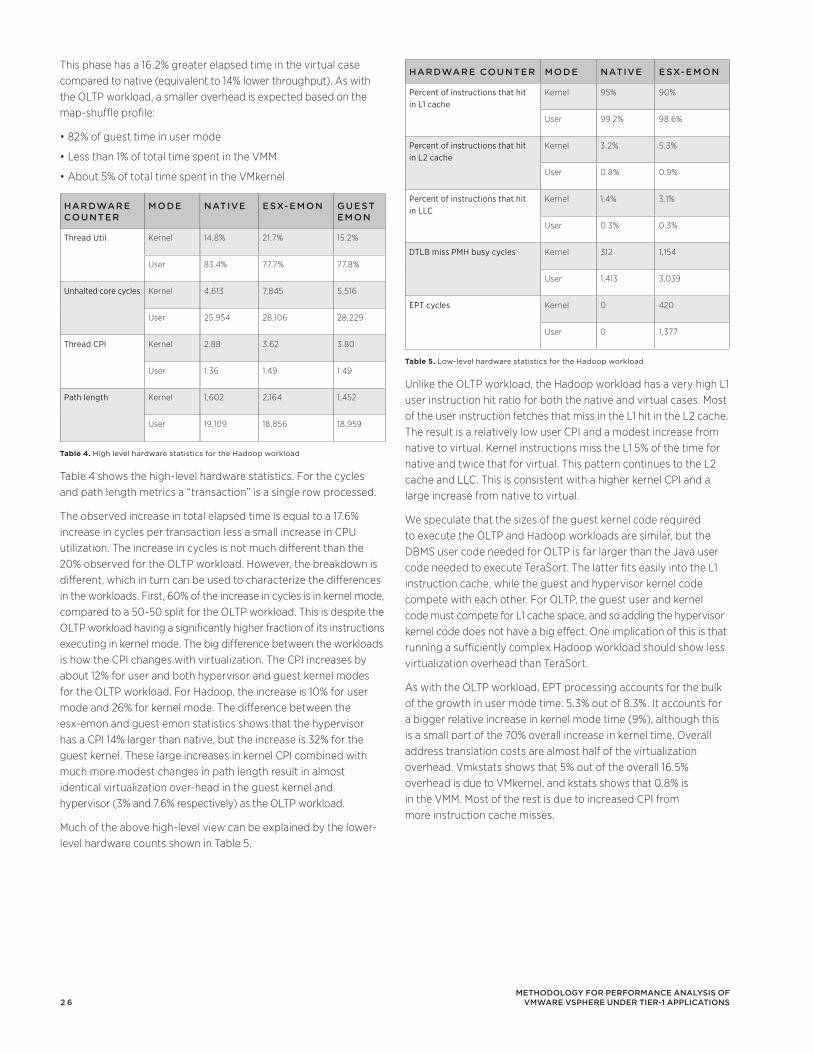
2 6

hardwarE cOuntEr MOdE natiVE ESX-EMOn


Kernel 95% 90%

User 99.2% 98.6%


Kernel 3.2% 5.3%

User 0.8% 0.9%

Percent of instructions that hit in LLC

Kernel 1.4% 3.1%

User 0.3% 0.3%

DTLB miss PMH busy cycles Kernel 312 1,154

User 1,413 3,039

EPT cycles Kernel 0 420

User 0 1,377

Table 5. Low-level hardware statistics for the Hadoop workload

Unlike the OLTP workload, the Hadoop workload has a very high L1 user instruction hit ratio for both the native and virtual cases. Most of the user instruction fetches that miss in the L1 hit in the L2 cache. The result is a relatively low user CPI and a modest increase from native to virtual. Kernel instructions miss the L1 5% of the time for native and twice that for virtual. This pattern continues to the L2 cache and LLC. This is consistent with a higher kernel CPI and a large increase from native to virtual.

We speculate that the sizes of the guest kernel code required to execute the OLTP and Hadoop workloads are similar, but the DBMS user code needed for OLTP is far larger than the Java user code needed to execute TeraSort. The latter fits easily into the L1 instruction cache, while the guest and hypervisor kernel code compete with each other. For OLTP, the guest user and kernel code must compete for L1 cache space, and so adding the hypervisor kernel code does not have a big effect. One implication of this is that running a sufficiently complex Hadoop workload should show less virtualization overhead than TeraSort.

As with the OLTP workload, EPT processing accounts for the bulk of the growth in user mode time: 5.3% out of 8.3%. It accounts for a bigger relative increase in kernel mode time (9%), although this is a small part of the 70% overall increase in kernel time. Overall address translation costs are almost half of the virtualization overhead. Vmkstats shows that 5% out of the overall 16.5% overhead is due to VMkernel, and kstats shows that 0.8% is in the VMM. Most of the rest is due to increased CPI from more instruction cache misses.

This phase has a 16.2% greater elapsed time in the virtual case compared to native (equivalent to 14% lower throughput). As with the OLTP workload, a smaller overhead is expected based on the map-shuffle profile:

•82%ofguesttimeinusermode

•Lessthan1%oftotaltimespentintheVMM

•About5%oftotaltimespentintheVMkernel

hardwarE cOuntEr


Thread Util Kernel 14.8% 21.7% 15.2%

User 83.4% 77.7% 77.8%

Unhalted core cycles Kernel 4,613 7,845 5,516

User 25,954 28,106 28,229

Thread CPI Kernel 2.88 3.62 3.80

User 1.36 1.49 1.49

Path length Kernel 1,602 2,164 1,452

User 19,109 18,856 18,959

Table 4. High level hardware statistics for the Hadoop workload

Table 4 shows the high-level hardware statistics. For the cycles and path length metrics a “transaction” is a single row processed.

The observed increase in total elapsed time is equal to a 17.6% increase in cycles per transaction less a small increase in CPU utilization. The increase in cycles is not much different than the 20% observed for the OLTP workload. However, the breakdown is different, which in turn can be used to characterize the differences in the workloads. First, 60% of the increase in cycles is in kernel mode, compared to a 50-50 split for the OLTP workload. This is despite the OLTP workload having a significantly higher fraction of its instructions executing in kernel mode. The big difference between the workloads is how the CPI changes with virtualization. The CPI increases by about 12% for user and both hypervisor and guest kernel modes for the OLTP workload. For Hadoop, the increase is 10% for user mode and 26% for kernel mode. The difference between the esx-emon and guest emon statistics shows that the hypervisor has a CPI 14% larger than native, but the increase is 32% for the guest kernel. These large increases in kernel CPI combined with much more modest changes in path length result in almost identical virtualization over-head in the guest kernel and hypervisor (3% and 7.6% respectively) as the OLTP workload.

Much of the above high-level view can be explained by the lower-level hardware counts shown in Table 5.


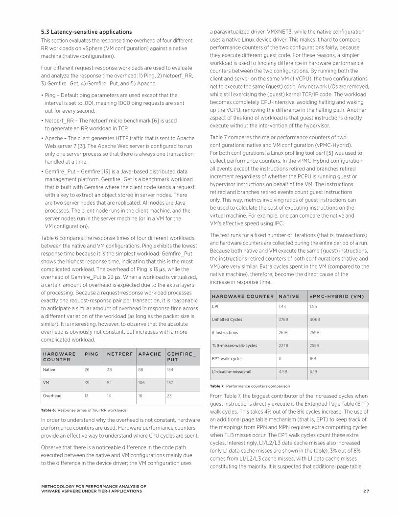
2 7

a paravirtualized driver, VMXNET3, while the native configuration uses a native Linux device driver. This makes it hard to compare performance counters of the two configurations fairly, because they execute different guest code. For these reasons, a simpler workload is used to find any difference in hardware performance counters between the two configurations. By running both the client and server on the same VM (1 VCPU), the two configurations get to execute the same (guest) code. Any network I/Os are removed, while still exercising the (guest) kernel TCP/IP code. The workload becomes completely CPU-intensive, avoiding halting and waking up the VCPU, removing the difference in the halting path. Another aspect of this kind of workload is that guest instructions directly execute without the intervention of the hypervisor.

Table 7 compares the major performance counters of two configurations: native and VM configuration (vPMC-Hybrid). For both configurations, a Linux profiling tool perf [5] was used to collect performance counters. In the vPMC-Hybrid configuration, all events except the instructions retired and branches retired increment regardless of whether the PCPU is running guest or hypervisor instructions on behalf of the VM. The instructions retired and branches retired events count guest instructions only. This way, metrics involving ratios of guest instructions can be used to calculate the cost of executing instructions on the virtual machine. For example, one can compare the native and VM’s effective speed using IPC.

The test runs for a fixed number of iterations (that is, transactions) and hardware counters are collected during the entire period of a run. Because both native and VM execute the same (guest) instructions, the instructions retired counters of both configurations (native and VM) are very similar. Extra cycles spent in the VM (compared to the native machine), therefore, become the direct cause of the increase in response time.

hardwarE cOuntEr natiVE vpMc-hybrid (VM)

CPI 1.43 1.56

Unhalted Cycles 376B 406B

# Instructions 261B 259B

TLB-misses-walk-cycles 227B 255B

EPT-walk-cycles 0 16B

L1-dcache-misses-all 4.5B 6.1B

Table 7. Performance counters comparison

From Table 7, the biggest contributor of the increased cycles when guest instructions directly execute is the Extended Page Table (EPT) walk cycles. This takes 4% out of the 8% cycles increase. The use of an additional page table mechanism (that is, EPT) to keep track of the mappings from PPN and MPN requires extra computing cycles when TLB misses occur. The EPT walk cycles count these extra cycles. Interestingly, L1/L2/L3 data cache misses also increased (only L1 data cache misses are shown in the table). 3% out of 8% comes from L1/L2/L3 cache misses, with L1 data cache misses constituting the majority. It is suspected that additional page table

5.3 Latency-sensitive applicationsThis section evaluates the response time overhead of four different RR workloads on vSphere (VM configuration) against a native machine (native configuration).

Four different request-response workloads are used to evaluate and analyze the response time overhead: 1) Ping, 2) Netperf_RR, 3) Gemfire_Get, 4) Gemfire_Put, and 5) Apache.

•Ping–Defaultpingparametersareusedexceptthatthe interval is set to .001, meaning 1000 ping requests are sent out for every second.

•Netperf_RR–TheNetperfmicrobenchmark[6]isused to generate an RR workload in TCP.

•Apache–TheclientgeneratesHTTPtrafficthatissenttoApacheWeb server 7 [3]. The Apache Web server is configured to run only one server process so that there is always one transaction handled at a time.

•Gemfire_Put–Gemfire[13]isaJava-baseddistributeddatamanagement platform. Gemfire_Get is a benchmark workload that is built with Gemfire where the client node sends a request with a key to extract an object stored in server nodes. There are two server nodes that are replicated. All nodes are Java processes. The client node runs in the client machine, and the server nodes run in the server machine (or in a VM for the VM configuration).

Table 6 compares the response times of four different workloads between the native and VM configurations. Ping exhibits the lowest response time because it is the simplest workload. Gemfire_Put shows the highest response time, indicating that this is the most complicated workload. The overhead of Ping is 13 µs, while the overhead of Gemfire_Put is 23 µs. When a workload is virtualized, a certain amount of overhead is expected due to the extra layers of processing. Because a request-response workload processes exactly one request-response pair per transaction, it is reasonable to anticipate a similar amount of overhead in response time across a different variation of the workload (as long as the packet size is similar). It is interesting, however, to observe that the absolute overhead is obviously not constant, but increases with a more complicated workload.

hardwarE cOuntEr

pinG nEtpErF apachE GEMFirE _put

Native 26 38 88 134

VM 39 52 106 157

Overhead 13 14 18 23

Table 6. Response times of four RR workloads

In order to understand why the overhead is not constant, hardware performance counters are used. Hardware performance counters provide an effective way to understand where CPU cycles are spent.

Observe that there is a noticeable difference in the code path executed between the native and VM configurations mainly due to the difference in the device driver; the VM configuration uses


2 8

References 1 Adams, Keith, and Agesen, Ole: “A Comparison of Software

and Hardware Techniques for x86 Virtualization”, Proceedings of AS-PLOS 2006.

2 Agesen, Ole: “Software and Hardware Techniques for x86 Virtualization”; http://www.vmware.com/files/pdf/software_hardware_tech_x86_virt.pdf, 2009

3 Apache HTTP Server Project. The Apache Software Foundation. http://httpd.apache.org

4 Serebrin, B., Hecht, D.: Virtualizing Performance Counters. 5th Workshop on System-level Virtualization for High Performance Computing 2011, Bordeaux, France

5 perf: Linux profiling with performance. https://perf.wiki.kernel.org/index.php/Main_Page

6 Netperf. www.netperf.org, 2011. http://www.netperf.org/netperf/

7 Performance Analysis Guide for Intel® Core™ i7 Processor and Intel® Xeon™ 5500 processors http://software.intel.com/sites/products/collateral/hpc/vtune/performance_analysis_guide.pdf

8 Performance Evaluation of Intel EPT Hardware Assist http://www.vmware.com/pdf/Perf_ESX_Intel-EPT-eval.pdf

9 TPC: Detailed TPC-C Description: http://www.tpc.org/tpcc/detail.asp

10 Virtualizing Performance Counters http://labs.vmware.com/publications/virtualizing-performance-counters

11 Virtualizing Performance-Critical Database Applications in VMware® vSphere™: http://www.vmware.com/pdf/Perf_ESX40_Oracle-eval.pdf

12 VMware Knowledge Base: Using Virtual CPU Performance Monitoring Counters. http://kb.vmware.com/selfservice/microsites/search.do?language=en_US&cmd=displayKC&externalId=2030221

13 VMware vFabric GemFire. VMware, Inc., 2012.

structures (EPT page tables) seemingly incur more memory accesses, increasing L1 data cache misses. An increase in TLB cache misses (excluding EPT walk cycles) takes the remaining 1% of the 8% increase. This is likely due to more memory accesses.

Assuming that the TLB miss rate remains the same (just for the sake of analysis) when executing guest instructions, the over-head caused by using EPT and associated cache misses become proportionally increased to the duration of the guest code execution. In other words, the longer the guest code runs, the more overhead will be shown in response time. This explains why there is a variable component in the response time overhead of virtualization.

6. Conclusions and Future DirectionsUsing a combination of well-known Linux performance monitoring commands, the traditional vSphere performance evaluation tools, and hardware monitoring tools, we have shown that all the workloads studied here exhibit similar performance profiles when virtualized:

•Theratiotonativeisgood,usuallyinexcessof80%.

•TheVMMandVMkerneloverheadsareminimal,exceptforthevery high I/O cases, where we see as much as 10% of the time spent in the VMkernel.

•Muchofthedifferencewithnativeisduetothetaxvirtualizationplaces on the hardware, specifically in traversing a two-level MMU.

•BesidesthedirectEPTcosts,thedualpagetablearchitectureincreases the contention for data caches, further contributing to the increase in CPI.

Besides the EPT costs, most of the virtualization overheads that we discovered in our study are small. They are easy to dismiss. Yet together, they add up to a total performance gap that requires attention.

7. AcknowledgementsMany individuals contributed to the work presented here. We would like to thank Shilpi Agarwal, Nikhil Bhatia, Ole Agesen, Qasim Ali, Seongbeom Kim, Jim Mattson, Priti Mishra, Jeffrey Sheldon, Lenin Singaravelu, Garrett Smith, and Haoqiang Zheng.


http://www.vmware.com/files/pdf/software_hardware_tech_x86_virt.pdf

http://www.vmware.com/files/pdf/software_hardware_tech_x86_virt.pdf

http://software.intel.com/sites/products/collateral/hpc/vtune/performance_analysis_guide.pdf

http://software.intel.com/sites/products/collateral/hpc/vtune/performance_analysis_guide.pdf

http://labs.vmware.com/publications/virtualizing-performance-counters

http://labs.vmware.com/publications/virtualizing-performance-counters

http://www.vmware.com/pdf/Perf_ESX40_Oracle-eval.pdf

http://www.vmware.com/pdf/Perf_ESX40_Oracle-eval.pdf

http://kb.vmware.com/selfservice/microsites/search.do?language=en_US&cmd=displayKC&externalId=2030221



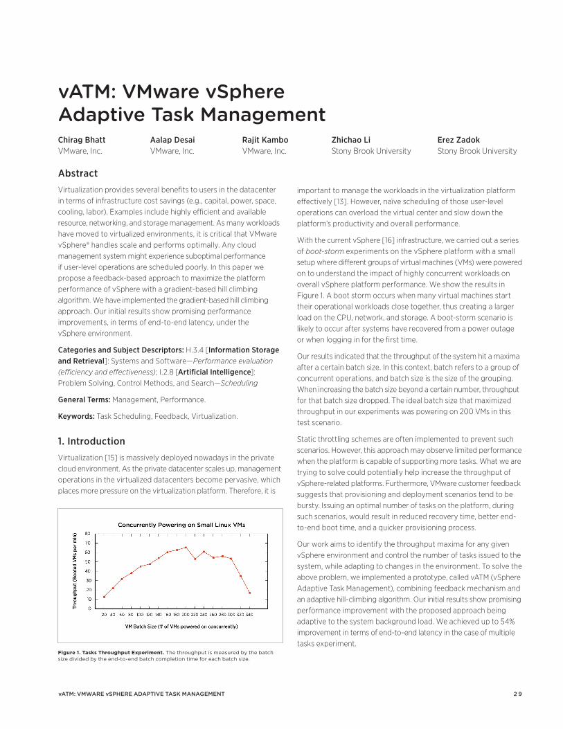
2 9

important to manage the workloads in the virtualization platform effectively [13]. However, naïve scheduling of those user-level operations can overload the virtual center and slow down the platform’s productivity and overall performance.

With the current vSphere [16] infrastructure, we carried out a series of boot-storm experiments on the vSphere platform with a small setup where different groups of virtual machines (VMs) were powered on to understand the impact of highly concurrent workloads on overall vSphere platform performance. We show the results in Figure 1. A boot storm occurs when many virtual machines start their operational workloads close together, thus creating a larger load on the CPU, network, and storage. A boot-storm scenario is likely to occur after systems have recovered from a power outage or when logging in for the first time.

Our results indicated that the throughput of the system hit a maxima after a certain batch size. In this context, batch refers to a group of concurrent operations, and batch size is the size of the grouping. When increasing the batch size beyond a certain number, throughput for that batch size dropped. The ideal batch size that maximized throughput in our experiments was powering on 200 VMs in this test scenario.

Static throttling schemes are often implemented to prevent such scenarios. However, this approach may observe limited performance when the platform is capable of supporting more tasks. What we are trying to solve could potentially help increase the throughput of vSphere-related platforms. Furthermore, VMware customer feedback suggests that provisioning and deployment scenarios tend to be bursty. Issuing an optimal number of tasks on the platform, during such scenarios, would result in reduced recovery time, better end-to-end boot time, and a quicker provisioning process.

Our work aims to identify the throughput maxima for any given vSphere environment and control the number of tasks issued to the system, while adapting to changes in the environment. To solve the above problem, we implemented a prototype, called vATM (vSphere Adaptive Task Management), combining feedback mechanism and an adaptive hill-climbing algorithm. Our initial results show promising performance improvement with the proposed approach being adaptive to the system background load. We achieved up to 54% improvement in terms of end-to-end latency in the case of multiple tasks experiment.

AbstractVirtualization provides several benefits to users in the datacenter in terms of infrastructure cost savings (e.g., capital, power, space, cooling, labor). Examples include highly efficient and available resource, networking, and storage management. As many workloads have moved to virtualized environments, it is critical that VMware vSphere® handles scale and performs optimally. Any cloud management system might experience suboptimal performance if user-level operations are scheduled poorly. In this paper we propose a feedback-based approach to maximize the platform performance of vSphere with a gradient-based hill climbing algorithm. We have implemented the gradient-based hill climbing approach. Our initial results show promising performance improvements, in terms of end-to-end latency, under the vSphere environment.

Categories and Subject Descriptors: H.3.4 [Information Storage and Retrieval]: Systems and Software—Performance evaluation (efficiency and effectiveness); I.2.8 [Artificial Intelligence]: Problem Solving, Control Methods, and Search—Scheduling

General Terms: Management, Performance.

Keywords: Task Scheduling, Feedback, Virtualization.

1. IntroductionVirtualization [15] is massively deployed nowadays in the private cloud environment. As the private datacenter scales up, management operations in the virtualized datacenters become pervasive, which places more pressure on the virtualization platform. Therefore, it is

vatM: VMware vSphere adaptive task ManagementChirag Bhatt Aalap Desai Rajit Kambo Zhichao Li Erez Zadok VMware, Inc. VMware, Inc. VMware, Inc. Stony Brook University Stony Brook University

vatM: vMware vSphere adaptive taSk ManageMent

Figure 1. Tasks Throughput Experiment. The throughput is measured by the batch size divided by the end-to-end batch completion time for each batch size.

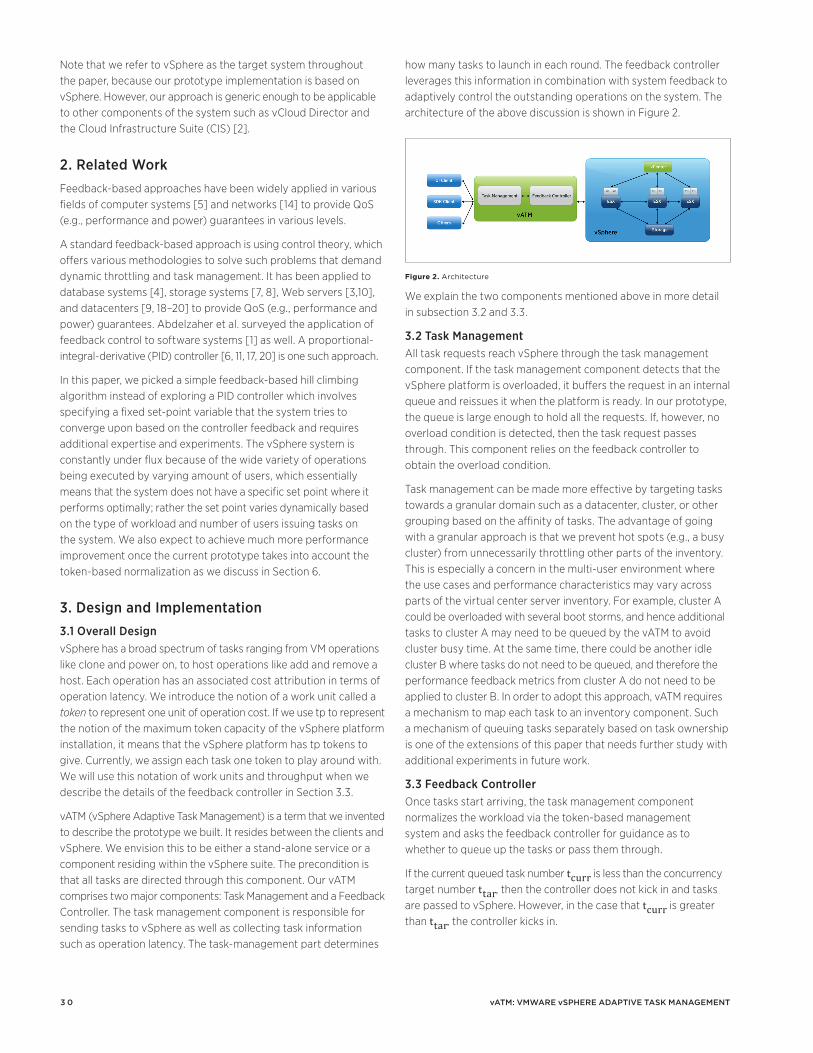
3 0

how many tasks to launch in each round. The feedback controller leverages this information in combination with system feedback to adaptively control the outstanding operations on the system. The architecture of the above discussion is shown in Figure 2.

We explain the two components mentioned above in more detail in subsection 3.2 and 3.3.

3.2 Task ManagementAll task requests reach vSphere through the task management component. If the task management component detects that the vSphere platform is overloaded, it buffers the request in an internal queue and reissues it when the platform is ready. In our prototype, the queue is large enough to hold all the requests. If, however, no overload condition is detected, then the task request passes through. This component relies on the feedback controller to obtain the overload condition.

Task management can be made more effective by targeting tasks towards a granular domain such as a datacenter, cluster, or other grouping based on the affinity of tasks. The advantage of going with a granular approach is that we prevent hot spots (e.g., a busy cluster) from unnecessarily throttling other parts of the inventory. This is especially a concern in the multi-user environment where the use cases and performance characteristics may vary across parts of the virtual center server inventory. For example, cluster A could be overloaded with several boot storms, and hence additional tasks to cluster A may need to be queued by the vATM to avoid cluster busy time. At the same time, there could be another idle cluster B where tasks do not need to be queued, and therefore the performance feedback metrics from cluster A do not need to be applied to cluster B. In order to adopt this approach, vATM requires a mechanism to map each task to an inventory component. Such a mechanism of queuing tasks separately based on task ownership is one of the extensions of this paper that needs further study with additional experiments in future work.

3.3 Feedback ControllerOnce tasks start arriving, the task management component normalizes the workload via the token-based management system and asks the feedback controller for guidance as to whether to queue up the tasks or pass them through.

If the current queued task number tcurr is less than the concurrency target number ttar, then the controller does not kick in and tasks are passed to vSphere. However, in the case that tcurr is greater than ttar, the controller kicks in.

Note that we refer to vSphere as the target system throughout the paper, because our prototype implementation is based on vSphere. However, our approach is generic enough to be applicable to other components of the system such as vCloud Director and the Cloud Infrastructure Suite (CIS) [2].

2. Related WorkFeedback-based approaches have been widely applied in various fields of computer systems [5] and networks [14] to provide QoS (e.g., performance and power) guarantees in various levels.

A standard feedback-based approach is using control theory, which offers various methodologies to solve such problems that demand dynamic throttling and task management. It has been applied to database systems [4], storage systems [7, 8], Web servers [3,10], and datacenters [9, 18–20] to provide QoS (e.g., performance and power) guarantees. Abdelzaher et al. surveyed the application of feedback control to software systems [1] as well. A proportional-integral-derivative (PID) controller [6, 11, 17, 20] is one such approach.

In this paper, we picked a simple feedback-based hill climbing algorithm instead of exploring a PID controller which involves specifying a fixed set-point variable that the system tries to converge upon based on the controller feedback and requires additional expertise and experiments. The vSphere system is constantly under flux because of the wide variety of operations being executed by varying amount of users, which essentially means that the system does not have a specific set point where it performs optimally; rather the set point varies dynamically based on the type of workload and number of users issuing tasks on the system. We also expect to achieve much more performance improvement once the current prototype takes into account the token-based normalization as we discuss in Section 6.

3. Design and Implementation3.1 Overall DesignvSphere has a broad spectrum of tasks ranging from VM operations like clone and power on, to host operations like add and remove a host. Each operation has an associated cost attribution in terms of operation latency. We introduce the notion of a work unit called a token to represent one unit of operation cost. If we use tp to represent the notion of the maximum token capacity of the vSphere platform installation, it means that the vSphere platform has tp tokens to give. Currently, we assign each task one token to play around with. We will use this notation of work units and throughput when we describe the details of the feedback controller in Section 3.3.

vATM (vSphere Adaptive Task Management) is a term that we invented to describe the prototype we built. It resides between the clients and vSphere. We envision this to be either a stand-alone service or a component residing within the vSphere suite. The precondition is that all tasks are directed through this component. Our vATM comprises two major components: Task Management and a Feedback Controller. The task management component is responsible for sending tasks to vSphere as well as collecting task information such as operation latency. The task-management part determines


Figure 2. Architecture

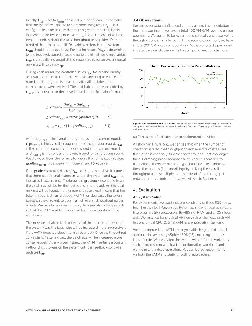
3 1

3.4 ObservationsCertain observations influenced our design and implementation. In the first experiment, we have in total 400 VM RAM reconfiguration operations. We launch 10 tasks per round statically and observe the throughput of each single round. In the second experiment, we have in total 200 VM power-on operations. We issue 10 tasks per round in a static way and observe the throughput of each single round.

(a) Throughput fluctuates due to background activities

As shown in Figure 3(a), we can see that when the number of operations is fixed, the throughput of each round fluctuates. This fluctuation is especially true for shorter rounds. That challenges the hill-climbing based approach a lot, since it is sensitive to fluctuations. Therefore, our prototype should be able to minimize these fluctuations (i.e., smoothing) by utilizing the overall throughput across multiple rounds instead of the throughput obtained from a single round, as we will see in Section 4.

4. Evaluation4.1 System SetupFor experiments, we used a cluster consisting of three ESX hosts. Each host is a Dell PowerEdge R610 machine with dual quad-core Intel Xeon 3.0GHz processors, 16–49GB of RAM, and 540GB local disk. We installed hundreds of VMs on each of the host. Each VM has one virtual CPU, 256MB RAM, and one 20GB virtual disk.

We implemented the vATM prototype with the gradient-based approach in Java using vSphere SDK [12] and using about 4K lines of code. We evaluated the system with different workloads such as boot-storm workload, reconfiguration workload, and workload with mixed operations. We carried out experiments via both the vATM and static throttling approaches.

Initially, ttar is set to tmin, the initial number of concurrent tasks that the system will handle to start processing tasks. tmin is a configurable value. In case that tcurr is greater than ttar, ttar is increased to be twice as much as tmin, in order to collect at least two data points about the task throughput to help identify the trend of the throughput hill. To avoid overshooting the system, tmin should not be too large. Further increase of ttar is determined by the feedback controller according to the hill-climbing mechanism. ttar is gradually increased till the system achieves an experimental maxima with capacity tp.

During each round, the controller issues ttar tasks concurrently and waits for them to complete. As tasks are completed in each round, the throughput is measured after all the tokens in the current round were received. The next batch size, represented by ttar+1, is increased or decreased based on the following formula:

where thpttar is the overall throughput as of the current round, thpttar−1 is the overall throughput as of the previous round, ttar is the number of concurrent tokens issued in the current round, and ttar−1 is the concurrent tokens issued for the previous round. We divide by 90 in the formula to ensure the normalized gradient gradientnorm is between −1 (inclusive) and 1 (exclusive).

If the gradient calculated across ttar and ttar−1 is positive, it suggests that there is additional headroom within the system and ttar+1 is increased in accordance. The larger the gradient value is, the larger the batch size will be for the next round, and the quicker the local maxima will be found. If the gradient is negative, it means that the token throughput has dropped: vATM then decreases the tokens based on the gradient, to obtain a high overall throughput across rounds. We set a floor value for the system available tokens as well, so that the vATM is able to launch at least one operation in the worst case.

The increase in batch size is reflective of the throughput trend of the system (e.g., the batch size will be increased more aggressively if the vATM detects a steep rise in throughput). Once the throughput curve starts flattening out, the batch size will be increased more conservatively. At any given instant, the vATM maintains a constant in-flow of ttar tokens on the system until the feedback controller updates ttar.


Figure 3. Fluctuation and variation. Observations with static throttling. A “round” is completed when batched concurrent tasks are finished. Throughput is measured for a single round.

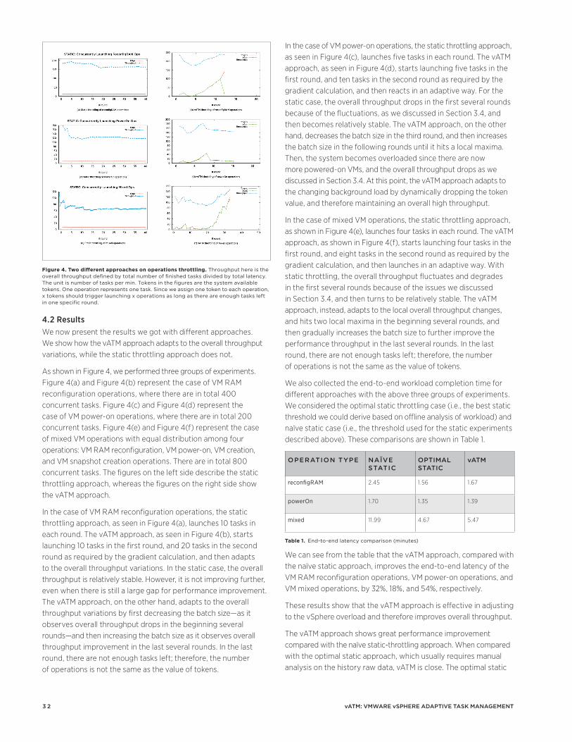
3 2

4.2 ResultsWe now present the results we got with different approaches. We show how the vATM approach adapts to the overall throughput variations, while the static throttling approach does not.

As shown in Figure 4, we performed three groups of experiments. Figure 4(a) and Figure 4(b) represent the case of VM RAM reconfiguration operations, where there are in total 400 concurrent tasks. Figure 4(c) and Figure 4(d) represent the case of VM power-on operations, where there are in total 200 concurrent tasks. Figure 4(e) and Figure 4(f) represent the case of mixed VM operations with equal distribution among four operations: VM RAM reconfiguration, VM power-on, VM creation, and VM snapshot creation operations. There are in total 800 concurrent tasks. The figures on the left side describe the static throttling approach, whereas the figures on the right side show the vATM approach.

In the case of VM RAM reconfiguration operations, the static throttling approach, as seen in Figure 4(a), launches 10 tasks in each round. The vATM approach, as seen in Figure 4(b), starts launching 10 tasks in the first round, and 20 tasks in the second round as required by the gradient calculation, and then adapts to the overall throughput variations. In the static case, the overall throughput is relatively stable. However, it is not improving further, even when there is still a large gap for performance improvement. The vATM approach, on the other hand, adapts to the overall throughput variations by first decreasing the batch size—as it observes overall throughput drops in the beginning several rounds—and then increasing the batch size as it observes overall throughput improvement in the last several rounds. In the last round, there are not enough tasks left; therefore, the number of operations is not the same as the value of tokens.

In the case of VM power-on operations, the static throttling approach, as seen in Figure 4(c), launches five tasks in each round. The vATM approach, as seen in Figure 4(d), starts launching five tasks in the first round, and ten tasks in the second round as required by the gradient calculation, and then reacts in an adaptive way. For the static case, the overall throughput drops in the first several rounds because of the fluctuations, as we discussed in Section 3.4, and then becomes relatively stable. The vATM approach, on the other hand, decreases the batch size in the third round, and then increases the batch size in the following rounds until it hits a local maxima. Then, the system becomes overloaded since there are now more powered-on VMs, and the overall throughput drops as we discussed in Section 3.4. At this point, the vATM approach adapts to the changing background load by dynamically dropping the token value, and therefore maintaining an overall high throughput.

In the case of mixed VM operations, the static throttling approach, as shown in Figure 4(e), launches four tasks in each round. The vATM approach, as shown in Figure 4(f), starts launching four tasks in the first round, and eight tasks in the second round as required by the gradient calculation, and then launches in an adaptive way. With static throttling, the overall throughput fluctuates and degrades in the first several rounds because of the issues we discussed in Section 3.4, and then turns to be relatively stable. The vATM approach, instead, adapts to the local overall throughput changes, and hits two local maxima in the beginning several rounds, and then gradually increases the batch size to further improve the performance throughput in the last several rounds. In the last round, there are not enough tasks left; therefore, the number of operations is not the same as the value of tokens.

We also collected the end-to-end workload completion time for different approaches with the above three groups of experiments. We considered the optimal static throttling case (i.e., the best static threshold we could derive based on offline analysis of workload) and naïve static case (i.e., the threshold used for the static experiments described above). These comparisons are shown in Table 1.

OpEratiOn typE naïVE Static

OptiMal Static

vatM

reconfigRAM 2.45 1.56 1.67

powerOn 1.70 1.35 1.39

mixed 11.99 4.67 5.47

Table 1. End-to-end latency comparison (minutes)

We can see from the table that the vATM approach, compared with the naïve static approach, improves the end-to-end latency of the VM RAM reconfiguration operations, VM power-on operations, and VM mixed operations, by 32%, 18%, and 54%, respectively.

These results show that the vATM approach is effective in adjusting to the vSphere overload and therefore improves overall throughput.

The vATM approach shows great performance improvement compared with the naïve static-throttling approach. When compared with the optimal static approach, which usually requires manual analysis on the history raw data, vATM is close. The optimal static


Figure 4. Two different approaches on operations throttling. Throughput here is the overall throughput defined by total number of finished tasks divided by total latency. The unit is number of tasks per min. Tokens in the figures are the system available tokens. One operation represents one task. Since we assign one token to each operation, x tokens should trigger launching x operations as long as there are enough tasks left in one specific round.

3 3

approach outperforms the vATM approach by 4% for VM RAM reconfiguration operations, 3% for VM power-on operations, and 7% for VM mixed operations, respectively. The reason is that the vATM approach takes some time to find the local maxima, as it starts launching tasks conservatively. We believe that with a large enough operation set, the time period the vATM takes to find the local maxima can be ignored, and the vATM approach will perform even better.

5. ConclusionIn this paper, we proposed one feedback-based approach aiming to maximize the vSphere platform performance with a gradient-based hill-climbing approach. We have implemented the gradient-based hill-climbing approach, and the results showed promising performance improvement under the vSphere environment. Compared with the naïve static approach, vATM improves the end-to-end latency of the VM RAM reconfiguration operations, VM power-on operations, and VM mixed operations by 32%, 18%, and 54%, respectively. Compared with the optimal static approach, vATM is close with 4% less for VM RAM reconfiguration operations, 3% less for VM power on operations, and 7% less for VM mixed operations, respectively.

6. Future WorkWe plan to assign tasks with dynamic tokens based on what the background load is at a specific time. We plan to integrate the token normalization approach, which normalizes each task token adaptively, into the vATM and collect some results with various task loads. We also plan to have a periodic intervention thread to update the system token in a more timely way in case there are any system metrics (e.g., system resource usage, individual operation latency, etc.) that vSphere has to abide to. This will prevent the hill-climbing approach from grossly overshooting the throughput hill. Besides, to further improve system throughput, we plan to enable launching tasks in the middle of each round once vATM observes task completeness and has enough system tokens to assign to additional tasks. Moreover, we plan to scale the experimental setup to perform larger tests, to understand the vATM behavior in the long run. Lastly, the current implementation considers task management at the entire vSphere level. However, going forward, we plan to use a more granular approach to manage tasks across both datacenters and clusters.

References1 T. F. Abdelzaher, J. A. Stankovic, C. Lu, R. Zhang, and Y. Lu.

Feedback performance control in software services. IEEE Control Systems Magazine, 23(3):74–90, 2003.

2 VMware Cloud Infrastructure Suite. http://www.vmware.com/cloud-infrastructure/business-critical-applications.html .

3 Y. Diao, N. Gandhi, J. L. Hellerstein, S. Parekh, and D. M. Tilbury. Using MIMO feedback control to enforce policies for interrelated metrics with application to the apache web server. In Proceedings of the Network Operations and Management Symposium, pages 219–234, 2002.

4 Y. Diao, J. L. Hellerstein, A. J. Storm, M. Surendra, S. Lightstone, S. Parekh, and C. Garcia-Arellano. Using MIMO linear control for load balancing in computing systems. In 2004 American Control Conferences, 2004.

5 P. C. Diniz and M. C. Rinard. Dynamic feedback: an effective technique for adaptive computing. ACM SIGPLAN Notices, pages 71 – 84, 1997.

6 J. L. Hellerstein, Y. Diao, S. Parekh, and D. M. Tibury. Feedback Control of Computing Systems. Wiley-IEEE Press, 2004.

7 M. Karlsson, C. Karamanolis, and X. Zhu. Triage: Performance differentiation for storage systems using adaptive control. ACM Trans. Storage, 1(4), 2005.

8 H. D. Lee, Y. J. Nam, K. J. Jung, S. G. Jung, and C. Park. Regulating I/O performance of shared storage with a control theoretical approach. In NASA/IEEE Conference on Mass Storage Systems and Technologies (MSST). IEEE Society Press, 2004.

9 H. C. Lim, S. Babu, and J. S. Chase. Automated control for elastic storage. In Proceeding of the 7th International Conference on Autonomic computing, ICAC ’10, pages 1–10. ACM, 2010.

10 Y. Lu, A. Saxena, and T. F. Abdelzaher. Differentiated caching services; a control-theoretical approach. In 21st International Conference on Distributed Computing Systems, pages 615–624, 2001.


http://www.vmware.com/cloud-infrastructure/business-critical-applications.html

http://www.vmware.com/cloud-infrastructure/business-critical-applications.html

3 4

16 VMware vSphere. http://en.wikipedia.org/wiki/VMware_vSphere .

17 Q.-G. Wang, Z. Ye, W.-J. Cai, and C.-C. Hang. PID Control For Multivariable Processes. Lecture Notes in Control and Information Sciences, Springer, March 2008.

18 X. Wang, M. Chen, and X. Fu. MIMO power control for high-density servers in an enclosure. IEEE Trans. Parallel Distrib. Syst., 21:1412–1426, 2010.

19 X. Wang and Y. Wang. Coordinating power control and performance management for virtualized server clusters. IEEE Trans. Parallel Distrib. Syst., 22:245–259, February 2011.

20 Y. Wang, X. Wang, M. Chen, and X. Zhu. Power-efficient response time guarantees for virtualized enterprise servers. In Proceedings of the 2008 Real-Time Systems Symposium, pages 303–312. IEEE Computer Society, 2008.

11 P. Padala, K. G. Shin, X. Zhu, M. Uysal, Z. Wang, S. Singhal, A. Merchant, and K. Salem. Adaptive control of virtualized resources in utility computing environments. In Proceedings of the European Conference on Computer Systems, pages 289–302, 2007.

12 VMware vSphere Web Services SDK. https://www.vmware.com/support/developer/vc-sdk/ .

13 V. Soundararajan and J. M. Anderson. The impact of management operations on the virtualized datacenter. Proceedings of the 37th Annual International Symposium on Computer Architecture (ISCA’10), pages 326 – 337, 2010.

14 A. S. Tanenbaum. Computer Networks, 4th Edition. Prentice Hall, 2002.

15 VMware, Inc. Understanding Full Virtualization, Paravirtualization, and Hardware Assist, 2007. www.vmware.com/files/pdf/VMware_paravirtualization.pdf .


3 5

applications, although with exponential complexity in network’s tree-width. Interactive models such as in [4] for incremental improvement of diagnosis do not allow complete automation of the management solutions and self-healing capabilities that adaptively learn and update system knowledge and react to environmental changes adequately.

The goal of the current IT management area is development of models, methods, and apparatus for estimation of dynamic performance normalcy of systems, their abnormality detection and control (which include misbehaving RC determination), bottleneck identification, change point detection, and other analytical capabilities.

The first step towards adaptive and universal solutions to these problems include measuring the business and its IT performance metrics (such as online users count and application response time) and thus creating the “data image” of the system containing devices, applications, and operating systems. At present, the quantitative monitoring of IT networks and data collection for the whole system in terms of various metrics (time series) is a common practice. The next stage, and the main technological and scientific challenge, is knowledge mining from reservoirs of measured data and its proactive application in fault management of systems. New mathematical and statistical methods and tools are needed to turn this data storage into real value for performance management of those systems. The latter includes a retrospective analysis of collected time series data and online decision making schemes based on that analysis. In this context, the identification of network faults and slow-downs, as well as their precursor’s detection, is the goal of those statistical tools.

Determination of a potential RC when IT systems are misbehaving is the primary solution our method and the corresponding engine provide. Our approach can also identify potential critical abnormality patterns in IT infrastructures. The study relies on statistical modeling of abnormality events’ lifetimes and their correlation in those infrastructures. At the same time, the study does not assume a contextual knowledge of systems or applications running in networks. In comparison with existing approaches, we adopt a totally data-driven approach that allows handling a large volume

AbstractA data-agnostic approach to automated problem (fault or change) root cause determination in complex IT systems based on monitoring and anomaly event data correlation is developed. It also includes a framework for identification of bottlenecks and black swan type issues in IT infrastructures. The relevant anomaly event correlation engine (AECE) is designed, prototyped, and successfully applied to data from real environments. This approach is based on a historical analysis of abnormality events (obtained by application of an IT management analytics) with their probabilistic correlations. The general theory that applies information measures between the random variables embodying those events is described, and a particular scenario is discussed. The method is capable of detecting origins of problems and generating real-time recommendations for their locations in a hierarchical system. Moreover, it allows localizing the bottleneck IT resources which are persisting causes of historical problems. The black swan type events are shown to be retrospectively identified and used in their risk estimation on-line. The technology and algorithms are based on statistical processing of virtual directed graphs produced from historical anomaly events.

KeywordsNetwork monitoring; fault management; anomaly detection; anomaly event; event correlation; root cause analysis; bottlenecks; black swans; pattern detection; probability; directed graph.

1. IntroductionModern economies and business services are running on complex, dynamic, and heterogeneous Information Technology (IT) infrastructures. Previous generation rule-based diagnostic tools and methods that are designed to maintain the “health” of those systems quickly become outdated and useless. Furthermore, managing today’s IT systems becomes increasingly complicated with the deployment of rapidly growing cloud computing services and virtualized environments.

Automated anomaly detection and related problem root cause (RC) localization in IT-based business processes are extremely important technological challenges. In such dynamic environments, statistical inference models are used. Bayesian networks are widely used (see [1]-[3] and references therein) for these and other inference

an anomaly Event correlation Engine: identifying root causes, bottlenecks, and black Swans in it EnvironmentsMazda A. Marvasti [email protected]

Arnak V. Poghosyan [email protected]

Ashot N. Harutyunyan [email protected]

Naira M. Grigoryan [email protected]

Management BU, VMware

an anoMaly event correlation engine: identifying root cauSeS, BottleneckS, and Black SwanS in it environMentS

3 6

of fault events and produces recommendations for highly probable root events and associated IT resources responsible for the out-of-normal situations. Other algorithms in this field (such as [4]) rely on heavy utilization of rules and topology knowledge of the applications or systems to enable effective recommendations for root problem identification and localization.

The methodology employed here relies on information measures applied on the system abnormality events space to create historical recommendation lists of components (resources) for identification and localization of RCs of malfunctions in the past. The current active events are then mapped into those historical lists to create active recommendations. What this algorithm produces is a set of RC lists rank-ordered based on a computed “likelihood index” that identifies the most probable RC event in the generated list and the whole events space. It is assumed that we have no knowledge of casual and other relationships in the environment. However, if the system topology information is available, it can be used to achieve a more contextual recommendation.

Here we treat two additional problems: system bottleneck identification and risk estimation of black swan type events.

Bottleneck identification is critical for improving the performance of resources which are hindering the functioning of networks in long term perspectives and are hidden in the whole anomaly history of those systems. Hence, bottleneck localization and redesign in large infrastructures prevent further causes of serious impacts on the system performance or lower their probability of occurrence.

The second problem we consider is online estimation of risk of black swan type events [5]. These events are extremely rare in occurrence, but very high in potential to destroy the system or significantly influence its functioning. This risk estimation can also be done based on the analysis of past behavior of the system being monitored and its projection onto the present with highly probable scenarios.

As mentioned, for our analysis we use the anomaly events historically produced on IT resources under monitoring and abnormality control. An example of such an analytics and software engine is the VMware vCenter Operations Manager that constructs and recognizes the normal behavioral patterns of various IT resources and raises alarms on “out-of-normal” situations in the system via dynamic process control or thresholding. This technology implements sophisticated statistical analysis for predicting the normalcy ranges of monitored data based on its category, variability, change point occurrence, and cyclicality. The reference [6] is an example of such a dynamic thresholding algorithm. Figure 1 illustrates a metric within predicted dynamic thresholds (DT) and illustrates the misbehaving areas subject to alarming as anomalies.

The correlation method adopted here is parametric, statistically counting for lifetimes of DT-based anomaly events. A similar event correlation method that is non-parametric and also applicable beyond the IT sphere is studied in [7] in the context of pattern detection in semi-structured data such as log files.

Event correlation techniques have been used over the past two and a half decades as a principle tool for integrated management in networks to detect causes of performance problems. The paper by Martin-Flatin et al [8] surveys the evolution of those techniques and challenges that need to be addressed in design of systems and algorithms for modern, complex, and tightly integrated networks. An early event correlation model, strictly deterministic, aimed at improving telecommunications networks surveillance and fault diagnosis is introduced by Jakobson and Weissman [9] (see also references therein). Its conceptual framework relies on, in particular, network topology. The systems designed within this kind of framework substantially restrict their applicability in fuzzy environments with growing capacities and depth requiring scalability and universality. On the other hand, a uniform framework employing casual correlation codebook formalism (problem is an encoded alarm set with decoding to identify the original problem) for network management is proposed by Kliger et al [10]. The codebook approach does not quickly adapt to changes in network configuration. An extended, single, rigorous, and conceptual framework for casual and temporal correlations was introduced by Hasan et al in [11].

In the context of the related work discussion above, the current research belongs to the temporal correlation framework. At the same time, we consider a general and universal abstraction of anomaly events that are not network-inherent with a defined collection of fault indications, but a statistically inferred dynamic normalcy range violations of IT resources indicating change against the system’s historically “representative” behavior. Those dynamic ranges are obtained by self-tunable learning from monitoring data. In other words, we introduce the highest possible degree of generality (fuzziness) in alarm correlation theory independently of any physical context, system topology, or expert knowledge inserted in causality relationships. Moreover, in our interpretation, a problem (fault or change) in an IT system is a bundle of alarms or statistical anomaly events that need to be addressed in an efficient manner, proactively preventing potential regression of a system state into a serious performance issue. (Alternatively, problems not necessarily yielding a malfunction should be learned, produce a warning, and have their impact estimated.) The shortest way to achieve the run-time problem elimination is inferring the root cause alarms with their high-to-low “ratings” to follow in system stabilization and recovery. These definitions encompass the models studied in prior related works. Our framework implies also that any infrastructural transformation, evolution, or variations in the background physical flows within the system, dynamically (statistically) update the alarm correlations.

As soon as the DT’s are historically constructed (recognized) for an IT process under monitoring, they can be projected into the future as prediction for time-based normalcy ranges. Any data point appearing above or below those thresholds (or, alternatively, a series of points consecutively staying at out-of-ranges) is an abnormality event that can be characterized by an ID triple: {Resource ID, Attribute ID, Symptom ID}. Under Resource ID we interpret any IT resource such as server, computer, etc. The Attribute ID identifies a specific process (metric, time-series) monitored for that resource (such as


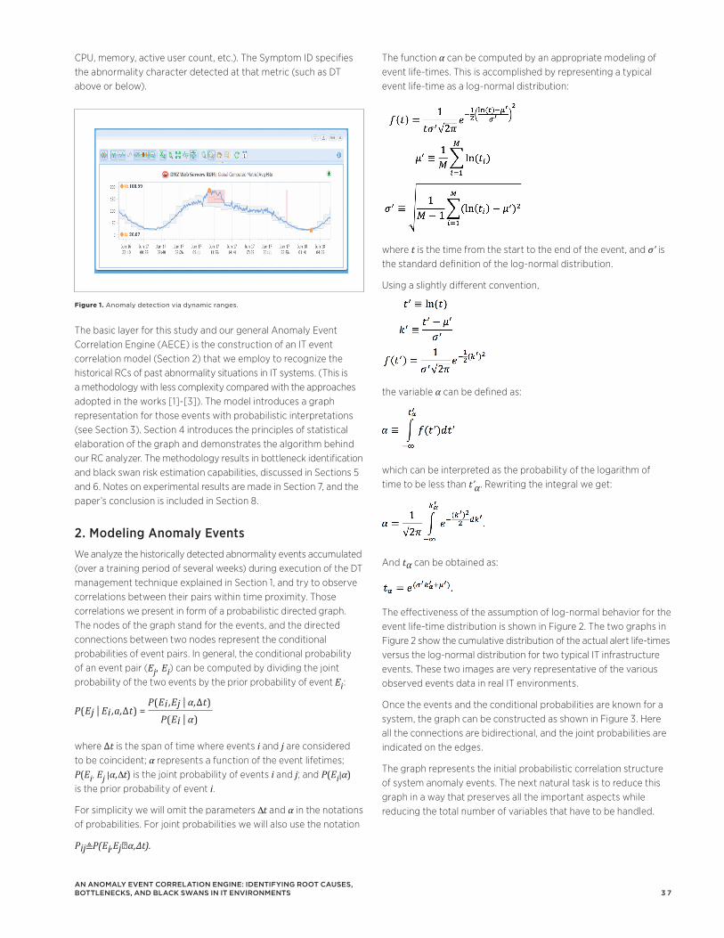
3 7

The function α can be computed by an appropriate modeling of event life-times. This is accomplished by representing a typical event life-time as a log-normal distribution:

where t is the time from the start to the end of the event, and σ’ is the standard definition of the log-normal distribution.

Using a slightly different convention,

the variable α can be defined as:

which can be interpreted as the probability of the logarithm of time to be less than t’α. Rewriting the integral we get:

And tα can be obtained as:

The effectiveness of the assumption of log-normal behavior for the event life-time distribution is shown in Figure 2. The two graphs in Figure 2 show the cumulative distribution of the actual alert life-times versus the log-normal distribution for two typical IT infrastructure events. These two images are very representative of the various observed events data in real IT environments.

Once the events and the conditional probabilities are known for a system, the graph can be constructed as shown in Figure 3. Here all the connections are bidirectional, and the joint probabilities are indicated on the edges.

The graph represents the initial probabilistic correlation structure of system anomaly events. The next natural task is to reduce this graph in a way that preserves all the important aspects while reducing the total number of variables that have to be handled.

CPU, memory, active user count, etc.). The Symptom ID specifies the abnormality character detected at that metric (such as DT above or below).

The basic layer for this study and our general Anomaly Event Correlation Engine (AECE) is the construction of an IT event correlation model (Section 2) that we employ to recognize the historical RCs of past abnormality situations in IT systems. (This is a methodology with less complexity compared with the approaches adopted in the works [1]-[3]). The model introduces a graph representation for those events with probabilistic interpretations (see Section 3). Section 4 introduces the principles of statistical elaboration of the graph and demonstrates the algorithm behind our RC analyzer. The methodology results in bottleneck identification and black swan risk estimation capabilities, discussed in Sections 5 and 6. Notes on experimental results are made in Section 7, and the paper’s conclusion is included in Section 8.

2. Modeling Anomaly EventsWe analyze the historically detected abnormality events accumulated (over a training period of several weeks) during execution of the DT management technique explained in Section 1, and try to observe correlations between their pairs within time proximity. Those correlations we present in form of a probabilistic directed graph. The nodes of the graph stand for the events, and the directed connections between two nodes represent the conditional probabilities of event pairs. In general, the conditional probability of an event pair (Ej, Ei) can be computed by dividing the joint probability of the two events by the prior probability of event Ei:

where ∆t is the span of time where events i and j are considered to be coincident; α represents a function of the event lifetimes; P(Ei, Ej |α,∆t) is the joint probability of events i and j; and P(Ei|α) is the prior probability of event i.

For simplicity we will omit the parameters ∆t and α in the notations of probabilities. For joint probabilities we will also use the notation

Pij P(Ei,Ej│α,∆t).


Figure 1. Anomaly detection via dynamic ranges.

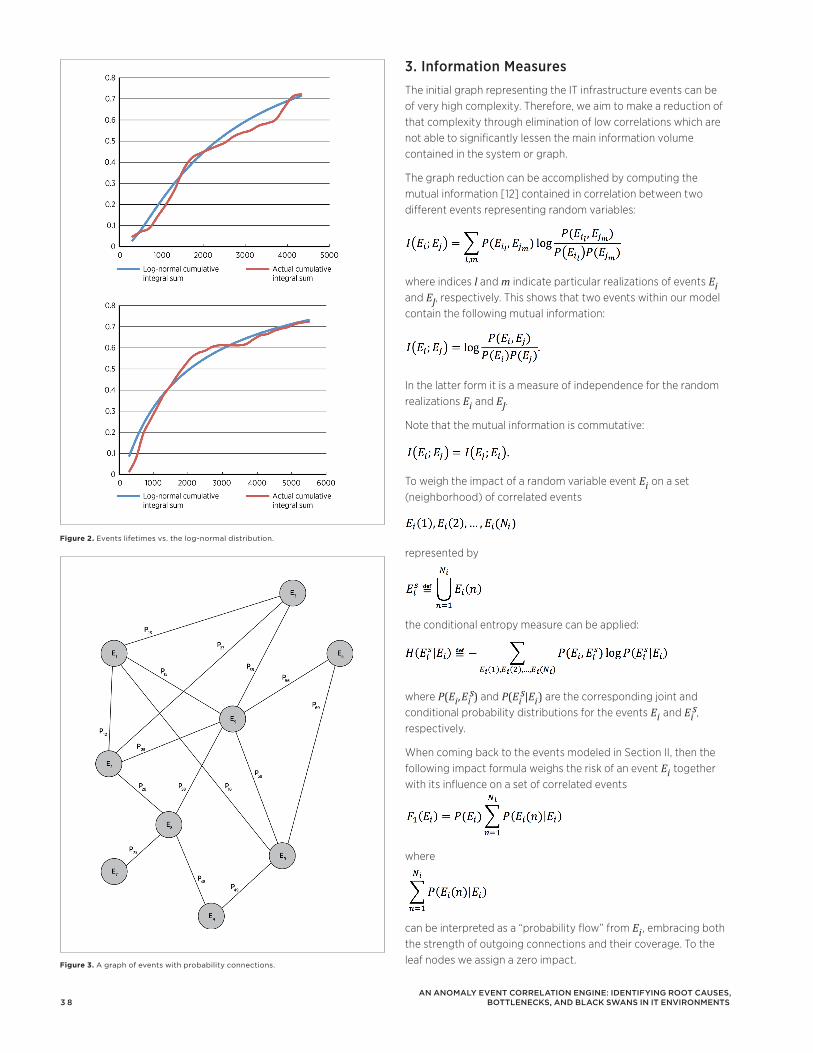
3 8

3. Information MeasuresThe initial graph representing the IT infrastructure events can be of very high complexity. Therefore, we aim to make a reduction of that complexity through elimination of low correlations which are not able to significantly lessen the main information volume contained in the system or graph.

The graph reduction can be accomplished by computing the mutual information [12] contained in correlation between two different events representing random variables:

where indices l and m indicate particular realizations of events Ei and EJ, respectively. This shows that two events within our model contain the following mutual information:

In the latter form it is a measure of independence for the random realizations Ei and EJ.

Note that the mutual information is commutative:

To weigh the impact of a random variable event Ei on a set (neighborhood) of correlated events

represented by

the conditional entropy measure can be applied:

where P(Ei ,Eis) and P(Ei

s|Ei) are the corresponding joint and conditional probability distributions for the events Ei and Ei

s, respectively.

When coming back to the events modeled in Section II, then the following impact formula weighs the risk of an event Ei together with its influence on a set of correlated events

where

can be interpreted as a “probability flow” from Ei , embracing both the strength of outgoing connections and their coverage. To the leaf nodes we assign a zero impact.


Figure 2. Events lifetimes vs. the log-normal distribution.

Figure 3. A graph of events with probability connections.

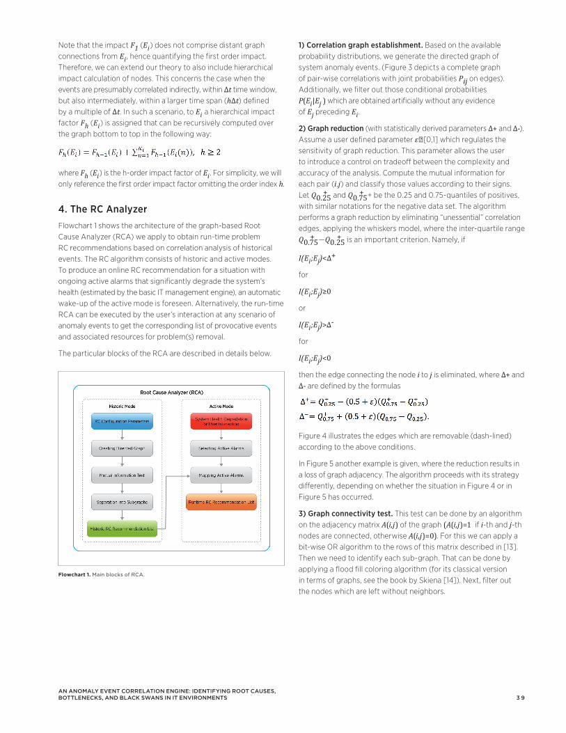
3 9

1) Correlation graph establishment. Based on the available probability distributions, we generate the directed graph of system anomaly events. (Figure 3 depicts a complete graph of pair-wise correlations with joint probabilities Pij on edges). Additionally, we filter out those conditional probabilities P(Ei|Ej ) which are obtained artificially without any evidence of Ej preceding Ei.

2) Graph reduction (with statistically derived parameters ∆+ and ∆-). Assume a user defined parameter ε∈[0,1] which regulates the sensitivity of graph reduction. This parameter allows the user to introduce a control on tradeoff between the complexity and accuracy of the analysis. Compute the mutual information for each pair (i,j) and classify those values according to their signs. Let Q0.25

+ and Q0.75+ + be the 0.25 and 0.75-quantiles of positives,

with similar notations for the negative data set. The algorithm performs a graph reduction by eliminating “unessential” correlation edges, applying the whiskers model, where the inter-quartile range Q0.75

+ —Q0.25+ is an important criterion. Namely, if

I(Ei;Ej)<∆+

for

I(Ei;Ej)≥0

or

I(Ei;Ej)>∆-

for

I(Ei;Ej)<0

then the edge connecting the node i to j is eliminated, where ∆+ and ∆- are defined by the formulas

Figure 4 illustrates the edges which are removable (dash-lined) according to the above conditions.

In Figure 5 another example is given, where the reduction results in a loss of graph adjacency. The algorithm proceeds with its strategy differently, depending on whether the situation in Figure 4 or in Figure 5 has occurred.

3) Graph connectivity test. This test can be done by an algorithm on the adjacency matrix A(i,j) of the graph (A(i,j)=1 if i-th and j-th nodes are connected, otherwise A(i,j)=0). For this we can apply a bit-wise OR algorithm to the rows of this matrix described in [13]. Then we need to identify each sub-graph. That can be done by applying a flood fill coloring algorithm (for its classical version in terms of graphs, see the book by Skiena [14]). Next, filter out the nodes which are left without neighbors.

Note that the impact F1 (Ei) does not comprise distant graph connections from Ei , hence quantifying the first order impact. Therefore, we can extend our theory to also include hierarchical impact calculation of nodes. This concerns the case when the events are presumably correlated indirectly, within ∆t time window, but also intermediately, within a larger time span (h∆t) defined by a multiple of ∆t. In such a scenario, to Ei a hierarchical impact factor Fh (Ei) is assigned that can be recursively computed over the graph bottom to top in the following way:

where Fh (Ei) is the h-order impact factor of Ei. For simplicity, we will only reference the first order impact factor omitting the order index h.

4. The RC Analyzer Flowchart 1 shows the architecture of the graph-based Root Cause Analyzer (RCA) we apply to obtain run-time problem RC recommendations based on correlation analysis of historical events. The RC algorithm consists of historic and active modes. To produce an online RC recommendation for a situation with ongoing active alarms that significantly degrade the system’s health (estimated by the basic IT management engine), an automatic wake-up of the active mode is foreseen. Alternatively, the run-time RCA can be executed by the user’s interaction at any scenario of anomaly events to get the corresponding list of provocative events and associated resources for problem(s) removal.

The particular blocks of the RCA are described in details below.


Flowchart 1. Main blocks of RCA.

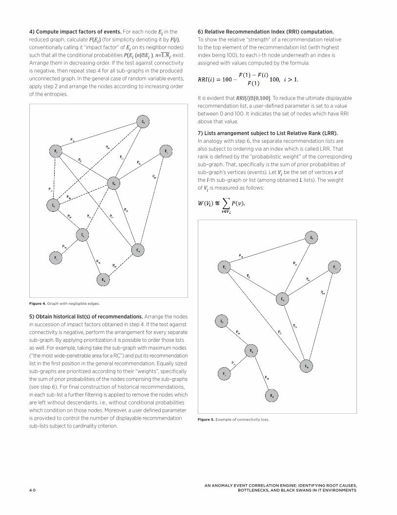
4 0

4) Compute impact factors of events. For each node Ei in the reduced graph, calculate F(Ei) (for simplicity denoting it by F(i), conventionally calling it “impact factor” of Ei on its neighbor nodes) such that all the conditional probabilities P(Ei (n)∈Ei ), n=1,Ni, exist. Arrange them in decreasing order. If the test against connectivity is negative, then repeat step 4 for all sub-graphs in the produced unconnected graph. In the general case of random variable events, apply step 2 and arrange the nodes according to increasing order of the entropies.

5) Obtain historical list(s) of recommendations. Arrange the nodes in succession of impact factors obtained in step 4. If the test against connectivity is negative, perform the arrangement for every separate sub-graph. By applying prioritization it is possible to order those lists as well. For example, taking take the sub-graph with maximum nodes (“the most wide-penetrable area for a RC”) and put its recommendation list in the first position in the general recommendation. Equally sized sub-graphs are prioritized according to their “weights”, specifically the sum of prior probabilities of the nodes comprising the sub-graphs (see step 6). For final construction of historical recommendations, in each sub-list a further filtering is applied to remove the nodes which are left without descendants, i.e., without conditional probabilities which condition on those nodes. Moreover, a user defined parameter is provided to control the number of displayable recommendation sub-lists subject to cardinality criterion.

6) Relative Recommendation Index (RRI) computation. To show the relative “strength” of a recommendation relative to the top element of the recommendation list (with highest index being 100), to each i-th node underneath an index is assigned with values computed by the formula:

It is evident that RRI(i)∈(0,100]. To reduce the ultimate displayable recommendation list, a user-defined parameter is set to a value between 0 and 100. It indicates the set of nodes which have RRI above that value.

7) Lists arrangement subject to List Relative Rank (LRR). In analogy with step 6, the separate recommendation lists are also subject to ordering via an index which is called LRR. That rank is defined by the “probabilistic weight” of the corresponding sub-graph. That, specifically is the sum of prior probabilities of sub-graph’s vertices (events). Let Vi be the set of vertices v of the l-th sub-graph or list (among obtained L lists). The weight of Vi is measured as follows:


Figure 4. Graph with negligible edges.

Figure 5. Example of connectivity loss.

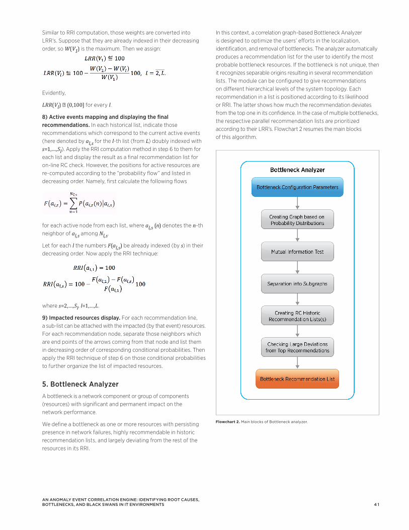
4 1

Similar to RRI computation, those weights are converted into LRR’s. Suppose that they are already indexed in their decreasing order, so W(V1) is the maximum. Then we assign:

Evidently,

LRR(Vl) ∈ (0,100] for every l.

8) Active events mapping and displaying the final recommendations. In each historical list, indicate those recommendations which correspond to the current active events (here denoted by al,s for the l-th list (from L) doubly indexed with s=1,…,Sl). Apply the RRI computation method in step 6 to them for each list and display the result as a final recommendation list for on-line RC check. However, the positions for active resources are re-computed according to the “probability flow” and listed in decreasing order. Namely, first calculate the following flows

for each active node from each list, where al,s (n) denotes the n-th neighbor of al,s among Nl,s.

Let for each l the numbers F(al,s) be already indexed (by s) in their decreasing order. Now apply the RRI technique:

where s=2,…,Sl, l=1,…,L.

9) Impacted resources display. For each recommendation line, a sub-list can be attached with the impacted (by that event) resources. For each recommendation node, separate those neighbors which are end points of the arrows coming from that node and list them in decreasing order of corresponding conditional probabilities. Then apply the RRI technique of step 6 on those conditional probabilities to further organize the list of impacted resources.

5. Bottleneck AnalyzerA bottleneck is a network component or group of components (resources) with significant and permanent impact on the network performance.

We define a bottleneck as one or more resources with persisting presence in network failures, highly recommendable in historic recommendation lists, and largely deviating from the rest of the resources in its RRI.

In this context, a correlation graph-based Bottleneck Analyzer is designed to optimize the users’ efforts in the localization, identification, and removal of bottlenecks. The analyzer automatically produces a recommendation list for the user to identify the most probable bottleneck resources. If the bottleneck is not unique, then it recognizes separable origins resulting in several recommendation lists. The module can be configured to give recommendations on different hierarchical levels of the system topology. Each recommendation in a list is positioned according to its likelihood or RRI. The latter shows how much the recommendation deviates from the top one in its confidence. In the case of multiple bottlenecks, the respective parallel recommendation lists are prioritized according to their LRR’s. Flowchart 2 resumes the main blocks of this algorithm.


Flowchart 2. Main blocks of Bottleneck analyzer.

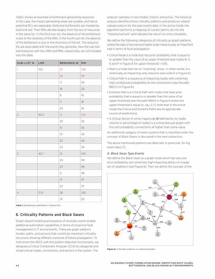
4 2

analyzer operates in two modes: historic and active. The historical analysis identifies those criticality patterns and produces related categorizations for the past events data. In the active mode, the algorithm performs a mapping of current alarms set into the “historical picture” and indicates the risk of run-time criticalities.

We define the following categories of criticality as graph patterns, where the idea of second and higher order impacts play an important role in terms of fault propagation:

•Critical Node is a node that has prior probability that is equal to or greater than the value of an upper threshold (see nodes B, G, K and P in Figure 6 for upper threshold = 0.9).

•Root is a node that has no “incoming” arrow ; in other words, it is historically an impacting-only resource (see node D in Figure 6).

•Critical Path is a sequence of impacting nodes with extremely high conditional probabilities on the connections (see the path BRSTU in Figure 6).

•Extreme Path is a Critical Path with nodes that have prior probability that is equal to or greater than the value of an upper threshold (see the path HBAO in Figure 6 where the upper threshold is equal to, say, 0.7). Note that in the active mode the Critical and Extreme Paths are an appropriate source of predictions).

•ACritical Sector of some magnitude M (defined by its nodes volume or percentage of nodes) is a connected sub-graph with the joint probability connections all higher than some value.

An additional category of event systems that is classified under the concept of Black Swans is discussed in the next subsection.

The above mentioned patterns are detected, in particular, for log event data [7].

A. Black Swan Type EventsWe define the Black Swan as a graph node which has very low prior probability, but extremely high impacting ability on a large set of neighbors (see Figure 6). Then we define the concept of the

Table I shows an example of bottleneck generating resources. In this case, the impact generating areas are isolable, and hence potential RCs are separable. Detected bottlenecks are marked by bold and red. Their RRIs deviate largely from the rest of resources in the same list. In the third sub-list, the absence of the bottleneck is due to the closeness of the RRIs. In the fourth sub-list, the absence of the bottleneck is due to the shortness of the list. The resource IDs are associated with the events they generate. Here the sub-lists and resources with low LRRs and RRIs, respectively, are not included into the table.

Sub-liSt n lrr rESOurcE id rri

1 100 27 100

26 99

17 98

18 20

8 18

11 18

25 18

2 90.2 14 100

24 56

15 55

10 40

32 40

33 39

3 40.7 12 100

29 99

23 98

9 98

13 97

22 97

4 21.9 28 100

19 50

Table 1: Bottlenecks identified in historic RL’s.

6. Criticality Patterns and Black SwansGraph-based modeling and analysis of anomaly events enable additional automation capabilities in terms of proactive fault management in IT environments. There are graph patterns (nodes, paths, and sectors) that constitute important criticality structures showing different scenarios of failure propagation. To instrument the AECE with this pattern detection functionality, we designed a Critical Component Analyzer (CCA) to categorize and reveal critical nodes, connections, and sectors in the system. The


Figure 6. Criticality patterns in a directed graph.

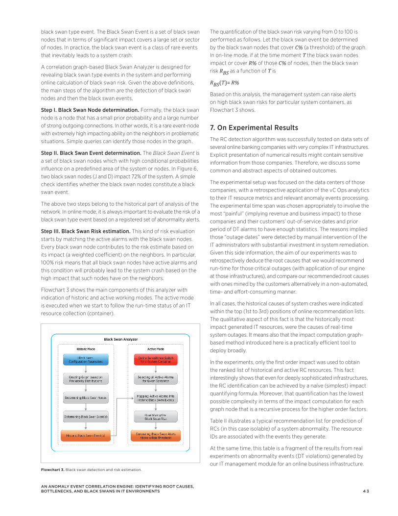
4 3

The quantification of the black swan risk varying from 0 to 100 is performed as follows. Let the black swan event be determined by the black swan nodes that cover C% (a threshold) of the graph. In on-line mode, if at the time moment T the black swan nodes impact or cover R% of those C% of nodes, then the black swan risk RBS as a function of T is

RBS(T)= R%

Based on this analysis, the management system can raise alerts on high black swan risks for particular system containers, as Flowchart 3 shows.

7. On Experimental ResultsThe RC detection algorithm was successfully tested on data sets of several online banking companies with very complex IT infrastructures. Explicit presentation of numerical results might contain sensitive information from those companies. Therefore, we discuss some common and abstract aspects of obtained outcomes.

The experimental setup was focused on the data centers of those companies, with a retrospective application of the vC Ops analytics to their IT resource metrics and relevant anomaly events processing. The experimental time span was chosen appropriately to involve the most “painful” (implying revenue and business impact) to those companies and their customers’ out-of-service dates and prior period of DT alarms to have enough statistics. The reasons implied those “outage dates” were detected by manual intervention of the IT administrators with substantial investment in system remediation. Given this side information, the aim of our experiments was to retrospectively deduce the root causes that we would recommend run-time for those critical outages (with application of our engine at those infrastructures), and compare our recommended root causes with ones mined by the customers alternatively in a non-automated, time- and effort-consuming manner.

In all cases, the historical causes of system crashes were indicated within the top (1st to 3rd) positions of online recommendation lists. The qualitative aspect of this fact is that the historically most impact generated IT resources, were the causes of real-time system outages. It means also that the impact computation graph-based method introduced here is a practically efficient tool to deploy broadly.

In the experiments, only the first order impact was used to obtain the ranked list of historical and active RC resources. This fact interestingly shows that even for deeply sophisticated infrastructures, the RC identification can be achieved by a naïve (simplest) impact quantifying formula. Moreover, that quantification has the lowest possible complexity in terms of the impact computation for each graph node that is a recursive process for the higher order factors.

Table II illustrates a typical recommendation list for prediction of RCs (in this case isolable) of a system abnormality. The resource IDs are associated with the events they generate.

At the same time, this table is a fragment of the results from real experiments on abnormality events (DT violations) generated by our IT management module for an online business infrastructure.

black swan type event. The Black Swan Event is a set of black swan nodes that in terms of significant impact covers a large set or sector of nodes. In practice, the black swan event is a class of rare events that inevitably leads to a system crash.

A correlation graph-based Black Swan Analyzer is designed for revealing black swan type events in the system and performing online calculation of black swan risk. Given the above definitions, the main steps of the algorithm are the detection of black swan nodes and then the black swan events.

Step I. Black Swan Node determination. Formally, the black swan node is a node that has a small prior probability and a large number of strong outgoing connections. In other words, it is a rare event-node with extremely high impacting ability on the neighbors in problematic situations. Simple queries can identify those nodes in the graph.

Step II. Black Swan Event determination. The Black Swan Event is a set of black swan nodes which with high conditional probabilities influence on a predefined area of the system or nodes. In Figure 6, two black swan nodes (J and D) impact 72% of the system. A simple check identifies whether the black swan nodes constitute a black swan event.

The above two steps belong to the historical part of analysis of the network. In online mode, it is always important to evaluate the risk of a black swan type event based on a registered set of abnormality alerts.

Step III. Black Swan Risk estimation. This kind of risk evaluation starts by matching the active alarms with the black swan nodes. Every black swan node contributes to the risk estimate based on its impact (a weighted coefficient) on the neighbors. In particular, 100% risk means that all black swan nodes have active alarms and this condition will probably lead to the system crash based on the high impact that such nodes have on the neighbors.

Flowchart 3 shows the main components of this analyzer with indication of historic and active working modes. The active mode is executed when we start to follow the run-time status of an IT resource collection (container).


Flowchart 3. Black swan detection and risk estimation.

4 4

8. ConclusionsWe introduced a new model of statistical inference for management of complex IT infrastructures based on their anomaly events data obtained from an intelligent monitoring engine. We demonstrated the components of the relevant prototyped module AECE that employs a directed virtual graph showing relationships and conditional probabilities between event pairs. An information-theoretic processing of this graph allows us to reliably predict the root causes of problems in IT systems. This technique was successfully applied to a number of data sets from real business environments running on very large IT infrastructures. The approach is also capable of identifying bottlenecks of network performance and evaluating the risk of black swan type events along with several other critical patterns.

References1 A. Alaeddini and I. Dogan, “Using Bayesian networks for root

cause analysis in statistical process control”, Expert Systems with Applications, vol. 38, issue 9, 2011, pp. 11230-11243.

2 S. Pradhan, R. Singh, K. Kachru, and S. Narasimhamurthy, “A Bayesian Network Based Approach for Root-Cause-Analysis in Manufacturing Process”, IEEE Int. Conf. on Computational Intelligence and Security, Harbin, China, Dec. 15-19, 2007, pp. 10-14.

3 S. Dey and J.A. Stori, “A Bayesian network approach to root cause diagnosis of process variations”, International Journal of Machine Tools and Manufacture, vol. 45, issue 1, 2004, pp. 75-91.

4 R.L. dos Santos, J.A. Wickboldt, R.C. Lunardi, B.L. Dalmazo, L.Z. Granville, L.P. Gaspary, C. Bartolini, and M. Hickey, “A solution for identifying the root cause of problems in IT change management”, Proc. Mini Conf. 12th IFIP/IEEE IM, Dublin, Ireland, May 23-27, 2011, pp. 586-593.

5 N.N. Taleb, The Black Swan: The Impact of the Highly Improbable, Random House, 2007.

6 M.A. Marvasti, A.V. Grigoryan, A.V. Poghosyan, N.M. Grigoryan, and A.N. Harutyunyan, “Methods for the cyclical pattern determination of time-series data using a clustering approach”, US patent application 20100036857, published 2010.

7 M.A. Marvasti, A.V. Poghosyan, A.N. Harutyunyan, and N.M. Grigoryan, “Pattern detection in unstructured data: An experience for a virtualized IT infrastructure”, to appear in Proc.IFIP/IEEE International Symposium on Integrated Network Management, Ghent, Belgium, May 27-31, 6 p., 2013.

Our methodology was able to correctly indicate the causes of a one-day system outage that significantly impacted the company’s business and its users’ activities. Here the sub-lists and resources with low LRRs and RRIs, respectively, are not included into the table.

For construction of the corresponding probabilistic graph, we processed more than 10,000 DT violation events registered during the monitoring and surveillance of this online banking company’s infrastructure over a two month period. Based on the historical RC lists derived from the correlation graph, we were able to produce the correct recommendation for problem localization at the time of system outage with a high number of alarming resources reported by our DT engine.

lrr rESOurcE id rri iMpactEd rESOurcES

100 8 100 9, 7, …

7 85.09 9, …

9 84.82 8, 7, …

67.4 5 100 6, …

6 80.86 …

Table II. Recommendation list with two sub-lists.

The recommendation lists can be consecutively refined via a user feedback option of the technology. In general, the algorithms shown above can be extended to incorporate user feedback information into the strategy to arrive at a better convergent solutions of the recommendations. This can be accomplished by asking the user a set of questions and appropriately modifying the algorithm with the user response. According to the answers, we assign different scores to the resources in recommendation lists to use in further computations.

The question that arises in using a purely data agnostic and statistical analysis is: Will the convergence of the answers to the actual RC be fast enough?

To accelerate the convergence, a user feedback mechanism is also incorporated which allows the algorithm to test the validity of its recommendation and improve its future recommendations. In general, the convergence rate is proportional to the RRI deviation of the desirable recommendation against the top recommendation.

In the same feedback context, further experimental insights can be achieved by monitoring and collecting statistics from users on their satisfaction with RC recommendations for everyday issues that are not necessarily serious system breakdowns.


4 5

11 M. Hasan, B. Sugla, and R. Viswanathan, “A conceptual framework for network management event correlation and filtering systems”, in Proc. 6th IFIP/IEEE International Symposium on Integrated Network Management (IM 1999), Boston, MA, USA, May 24-28, 1999, pp. 233–246.

12 T.M. Cover and J.A. Thomas, Elements of Information Theory, Wiley, 1991.

13 N. Deo, Graph Theory with Applications to Engineering and Computer Science, Prentice Hall, 1974.

14 S.S. Skiena, The Algorithm Design Manual, Springer, 2008.

8 J.P. Martin-Flatin, G. Jakobson and L. Lewis, “Event correlation in integrated management: Lessons learned and outlook”, Journal of Network and Systems Management, vol. 17, no. 4, December 2007.

9 G. Jakobson and M. Weissman, “Alarm correlation”, IEEE Network, vol. 7, no. 6, pp. 52–59, November 1993.

10 S. Kliger, S. Yemini, Y. Yemini, D. Ohsie and S. Stolfo, “A coding approach to event correlation”, in Proc. 4th IEEE/IFIP International Symposium on Integrated Network Management (ISINM 1995), Santa Barbara, CA, USA, May 1-5, 1995, pp. 266–277.


4 6

1. IntroductionWhen Facebook [3] introduced its search feature, it marked a watershed moment in web search. The Facebook database is a vast source of information that has deep relevance to its users. While Google has access to a similarly vast and important database of information, this information is not as specific to the users as the personal information in Facebook. One important distinction between search in Facebook and Google is the type of data involved. Facebook is not trying to create a generic search engine for all data; rather, it is capitalizing on the sort of data that is stored, namely, connectivity data in the form of a large, distributed graph database [2]. In the case of Facebook, the type of data stored (connectivity data) is well-matched to the mechanism of storage (a graph database).

Why is Facebook search useful? It is useful because it connects people with the information they really care about, namely, personal data. For example, a question like “Find all of my friends that ski” cannot be answered with a pure Google search, but can be answered using data from a social media database (whether it be Facebook or Google+ [1]). A Google search is extremely useful for purely factual information, but often less useful for queries that are of a more personal nature.

In a similar way, a virtualization infrastructure has a wide variety of information of interest to the virtualization administrator. This data is currently organized using a combination of a relational database (the virtualization management database) and an XML database (an embedded inventory service). However, similar to a Facebook search, many questions of interest to an administrator can be couched simply in terms of the connectivity graph for the virtual inventory. For example, an administrator may wish to know the answer to the question “Is there an administrator with access to both datastore X as well as VM Y?” This question can easily be answered via well-structured API calls to the virtualization manager (for example, VMware vSphere [13]), with vSphere performing the appropriate queries to its relational database. However, an extremely simplistic graph database can answer the question much more easily, and such a query can be expressed more intuitively. Moreover, it can be extended to answer a large number of other queries fairly easily.

In this paper, we propose reorganizing virtualization inventory data into a graph database, combining it with relationships from social media, and using this connectivity structure to address many virtualization administrator pain points. We discuss results from a preliminary prototype, and describe areas of future work leveraging this computing model.

AbstractFacebook graph search allows arbitrary queries that leverage the vast amount of information available in Facebook. With such a treasure trove of information, it is possible to answer a large number of questions like “find all of my friends that ski.” Such queries leverage this specialized Facebook database. Moreover, these answers are unavailable through other conventional search interfaces like Google. In a similar way, the database in a virtualized infrastructure can also be thought of as containing graph information: namely, the relationships between various entities like hosts, VMs, and datacenters. Many questions of interest to an administrator can be answered easily when couched in terms of a graph database. For example, suppose a customer would like to know how many VMs have disks that span multiple storage arrays, or which datastore is most critical (because it has the most VMs and hosts on it). These questions can be expressed simply in terms of graph traversal. However, VMware vSphere® currently has no simple interface to answer these sorts of questions. Why not use such graph search to help with virtualization management?

In this paper, we propose coupling the virtualization management API, graph search, and social media in order to provide an easy-to-use portal for answering a wide variety of graph-oriented management questions in a virtualized environment. We expand upon previous work in social media approaches to virtualization management and use the metaphors of social media to define simplified relationships between entities (for example, follower/followee relationships and group membership). We use the VMware virtualization management API to define the entities (for example, VMs and hosts) and relationships (for example, datastore or network connectivity), and we populate a VMware Socialcast® social media portal with such data. Finally, we import the resulting graph into a graph database and leverage easy-to-use query languages and interfaces to access these graphs and answer common management questions. We show examples from a preliminary prototype to demonstrate the usefulness of such an approach and also describe other use cases that leverage this sort of data organization.

Categories and Subject Descriptors: D.m [Miscellaneous]: Virtual Machines, system management, cloud computing.

General Terms: Performance, Management, Design.

Keywords: Virtual Machine management, cloud computing, datacenter management tools.

SiMplifying virtualization ManageMent with graph dataBaSeS

Simplifying Virtualization Management with Graph databasesVijayaraghavan Soundararajan Performance Group, VMware [email protected]

Lawrence Spracklen* Ayasdi [email protected]

1 Lawrence Spracklen was a VMware employee when working on this project.

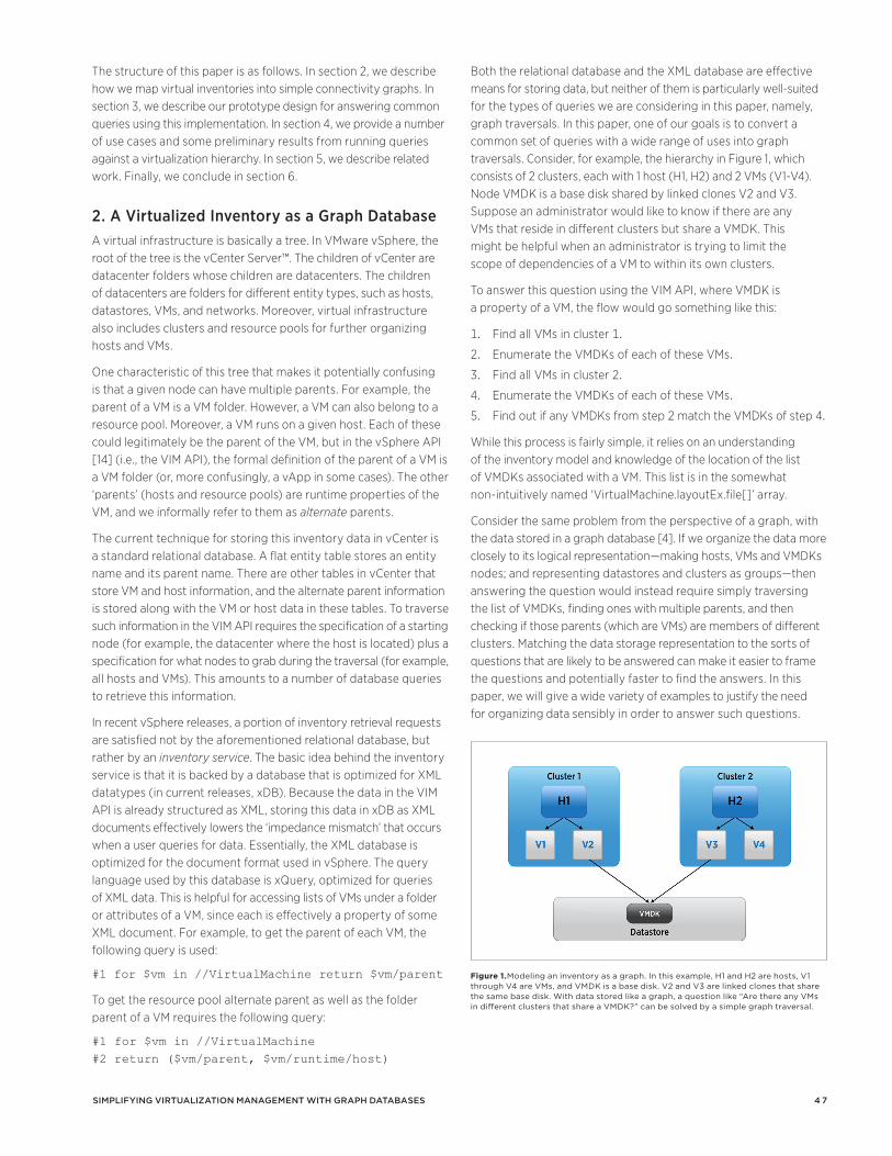
4 7

Both the relational database and the XML database are effective means for storing data, but neither of them is particularly well-suited for the types of queries we are considering in this paper, namely, graph traversals. In this paper, one of our goals is to convert a common set of queries with a wide range of uses into graph traversals. Consider, for example, the hierarchy in Figure 1, which consists of 2 clusters, each with 1 host (H1, H2) and 2 VMs (V1-V4). Node VMDK is a base disk shared by linked clones V2 and V3. Suppose an administrator would like to know if there are any VMs that reside in different clusters but share a VMDK. This might be helpful when an administrator is trying to limit the scope of dependencies of a VM to within its own clusters.

To answer this question using the VIM API, where VMDK is a property of a VM, the flow would go something like this:

1. Find all VMs in cluster 1.

2. Enumerate the VMDKs of each of these VMs.

3. Find all VMs in cluster 2.

4. Enumerate the VMDKs of each of these VMs.

5. Find out if any VMDKs from step 2 match the VMDKs of step 4.

While this process is fairly simple, it relies on an understanding of the inventory model and knowledge of the location of the list of VMDKs associated with a VM. This list is in the somewhat non-intuitively named ‘VirtualMachine.layoutEx.file[]’ array.

Consider the same problem from the perspective of a graph, with the data stored in a graph database [4]. If we organize the data more closely to its logical representation—making hosts, VMs and VMDKs nodes; and representing datastores and clusters as groups—then answering the question would instead require simply traversing the list of VMDKs, finding ones with multiple parents, and then checking if those parents (which are VMs) are members of different clusters. Matching the data storage representation to the sorts of questions that are likely to be answered can make it easier to frame the questions and potentially faster to find the answers. In this paper, we will give a wide variety of examples to justify the need for organizing data sensibly in order to answer such questions.

The structure of this paper is as follows. In section 2, we describe how we map virtual inventories into simple connectivity graphs. In section 3, we describe our prototype design for answering common queries using this implementation. In section 4, we provide a number of use cases and some preliminary results from running queries against a virtualization hierarchy. In section 5, we describe related work. Finally, we conclude in section 6.

2. A Virtualized Inventory as a Graph DatabaseA virtual infrastructure is basically a tree. In VMware vSphere, the root of the tree is the vCenter Server™. The children of vCenter are datacenter folders whose children are datacenters. The children of datacenters are folders for different entity types, such as hosts, datastores, VMs, and networks. Moreover, virtual infrastructure also includes clusters and resource pools for further organizing hosts and VMs.

One characteristic of this tree that makes it potentially confusing is that a given node can have multiple parents. For example, the parent of a VM is a VM folder. However, a VM can also belong to a resource pool. Moreover, a VM runs on a given host. Each of these could legitimately be the parent of the VM, but in the vSphere API [14] (i.e., the VIM API), the formal definition of the parent of a VM is a VM folder (or, more confusingly, a vApp in some cases). The other ‘parents’ (hosts and resource pools) are runtime properties of the VM, and we informally refer to them as alternate parents.

The current technique for storing this inventory data in vCenter is a standard relational database. A flat entity table stores an entity name and its parent name. There are other tables in vCenter that store VM and host information, and the alternate parent information is stored along with the VM or host data in these tables. To traverse such information in the VIM API requires the specification of a starting node (for example, the datacenter where the host is located) plus a specification for what nodes to grab during the traversal (for example, all hosts and VMs). This amounts to a number of database queries to retrieve this information.

In recent vSphere releases, a portion of inventory retrieval requests are satisfied not by the aforementioned relational database, but rather by an inventory service. The basic idea behind the inventory service is that it is backed by a database that is optimized for XML datatypes (in current releases, xDB). Because the data in the VIM API is already structured as XML, storing this data in xDB as XML documents effectively lowers the ‘impedance mismatch’ that occurs when a user queries for data. Essentially, the XML database is optimized for the document format used in vSphere. The query language used by this database is xQuery, optimized for queries of XML data. This is helpful for accessing lists of VMs under a folder or attributes of a VM, since each is effectively a property of some XML document. For example, to get the parent of each VM, the following query is used:

#1 for $vm in //VirtualMachine return $vm/parent

To get the resource pool alternate parent as well as the folder parent of a VM requires the following query:

#1 for $vm in //VirtualMachine

#2 return ($vm/parent, $vm/runtime/host)


Figure 1.Modeling an inventory as a graph. In this example, H1 and H2 are hosts, V1 through V4 are VMs, and VMDK is a base disk. V2 and V3 are linked clones that share the same base disk. With data stored like a graph, a question like “Are there any VMs in different clusters that share a VMDK?” can be solved by a simple graph traversal.

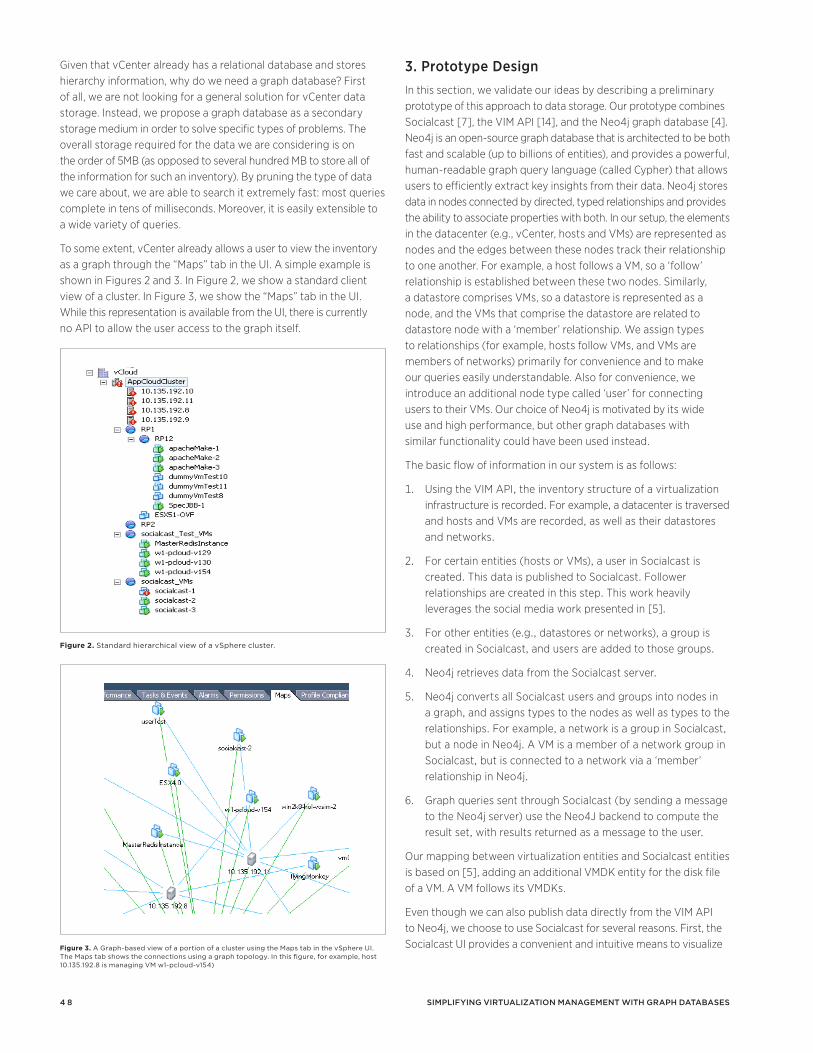
4 8

3. Prototype DesignIn this section, we validate our ideas by describing a preliminary prototype of this approach to data storage. Our prototype combines Socialcast [7], the VIM API [14], and the Neo4j graph database [4]. Neo4j is an open-source graph database that is architected to be both fast and scalable (up to billions of entities), and provides a powerful, human-readable graph query language (called Cypher) that allows users to efficiently extract key insights from their data. Neo4j stores data in nodes connected by directed, typed relationships and provides the ability to associate properties with both. In our setup, the elements in the datacenter (e.g., vCenter, hosts and VMs) are represented as nodes and the edges between these nodes track their relationship to one another. For example, a host follows a VM, so a ‘follow’ relationship is established between these two nodes. Similarly, a datastore comprises VMs, so a datastore is represented as a node, and the VMs that comprise the datastore are related to datastore node with a ‘member’ relationship. We assign types to relationships (for example, hosts follow VMs, and VMs are members of networks) primarily for convenience and to make our queries easily understandable. Also for convenience, we introduce an additional node type called ‘user’ for connecting users to their VMs. Our choice of Neo4j is motivated by its wide use and high performance, but other graph databases with similar functionality could have been used instead.

The basic flow of information in our system is as follows:

1. Using the VIM API, the inventory structure of a virtualization infrastructure is recorded. For example, a datacenter is traversed and hosts and VMs are recorded, as well as their datastores and networks.

2. For certain entities (hosts or VMs), a user in Socialcast is created. This data is published to Socialcast. Follower relationships are created in this step. This work heavily leverages the social media work presented in [5].

3. For other entities (e.g., datastores or networks), a group is created in Socialcast, and users are added to those groups.

4. Neo4j retrieves data from the Socialcast server.

5. Neo4j converts all Socialcast users and groups into nodes in a graph, and assigns types to the nodes as well as types to the relationships. For example, a network is a group in Socialcast, but a node in Neo4j. A VM is a member of a network group in Socialcast, but is connected to a network via a ‘member’ relationship in Neo4j.

6. Graph queries sent through Socialcast (by sending a message to the Neo4j server) use the Neo4J backend to compute the result set, with results returned as a message to the user.

Our mapping between virtualization entities and Socialcast entities is based on [5], adding an additional VMDK entity for the disk file of a VM. A VM follows its VMDKs.

Even though we can also publish data directly from the VIM API to Neo4j, we choose to use Socialcast for several reasons. First, the Socialcast UI provides a convenient and intuitive means to visualize

Given that vCenter already has a relational database and stores hierarchy information, why do we need a graph database? First of all, we are not looking for a general solution for vCenter data storage. Instead, we propose a graph database as a secondary storage medium in order to solve specific types of problems. The overall storage required for the data we are considering is on the order of 5MB (as opposed to several hundred MB to store all of the information for such an inventory). By pruning the type of data we care about, we are able to search it extremely fast: most queries complete in tens of milliseconds. Moreover, it is easily extensible to a wide variety of queries.

To some extent, vCenter already allows a user to view the inventory as a graph through the “Maps” tab in the UI. A simple example is shown in Figures 2 and 3. In Figure 2, we show a standard client view of a cluster. In Figure 3, we show the “Maps” tab in the UI. While this representation is available from the UI, there is currently no API to allow the user access to the graph itself.


Figure 2. Standard hierarchical view of a vSphere cluster.

Figure 3. A Graph-based view of a portion of a cluster using the Maps tab in the vSphere UI. The Maps tab shows the connections using a graph topology. In this figure, for example, host 10.135.192.8 is managing VM w1-pcloud-v154)

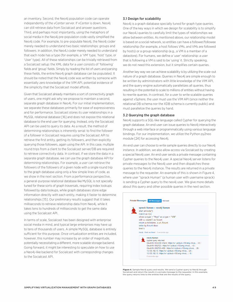
4 9

an inventory. Second, the Neo4j population code can operate independently of the vCenter server. If vCenter is down, Neo4j can still retrieve data from Socialcast and answer questions. Third, and perhaps most importantly, using the metaphors of social media in the Neo4j pre-population code vastly simplified the Neo4j code. For example, to pre-populate Neo4j, the Neo4j coder merely needed to understand two basic relationships: groups and followers. In addition, the Neo4J coder merely needed to understand that each node has a type (for example, a ‘VM’ type, ‘host’ type, or ‘User’ type). All of these relationships can be trivially retrieved from a Socialcast setup: the XML data for a user consists of ‘following’ fields and ‘group’ fields. Simply by reading the list of users and parsing these fields, the entire Neo4j graph database can be populated. It should be noted that the Neo4j code was written by someone with essentially zero knowledge of the VIM API, potential evidence of the simplicity that the Socialcast model affords.

Given that Socialcast already maintains a sort of connectivity graph of users, one might ask why we propose to maintain a second, separate graph database in Neo4j. For our initial implementation, we separate these databases primarily for ease of expressiveness and for performance. Socialcast stores its user relationships in a MySQL relational database [16] and does not expose this relational database to the end user for querying. Instead, only the Socialcast API can be used to query its data. As a result, the method of determining relationships is inherently serial: to find the follower of a follower in Socialcast requires using the Socialcast API to retrieve the first entity, getting its followers, and then explicitly querying those followers, again using the API. In this case, multiple round trips from a client to the Socialcast server/DB are required to retrieve connectivity data. In contrast, if we store the data in a separate graph database, we can use the graph database API for determining relationships. For example, a user can retrieve the followers of the followers of a given node with a single round trip to the graph database using only a few simple lines of code, as we show in the next section. From a performance perspective, a general-purpose relational database like MySQL is not specially tuned for these sorts of graph traversals, requiring index lookups followed by data lookups, while graph databases store edge information directly with each entity, making it faster to determine relationships [15]. Our preliminary results suggest that it takes milliseconds to retrieve relationship data from Neo4j, while it takes tens to hundreds of milliseconds to get the same data using the Socialcast API.

In terms of scale, Socialcast has been designed with enterprise social media in mind, and typical large enterprises may have up to tens of thousands of users. A simple MySQL database is entirely sufficient for this purpose. Once virtualization entities are included, however, this number may increase by an order of magnitude, potentially necessitating a different, more scalable storage backend. Going forward, it might be interesting to speculate on how to use a Neo4j-like backend for Socialcast with corresponding changes to the Socialcast API.

3.1 Design for scalabilityNeo4j is a graph database specially tuned for graph type queries. One of the key ways in which we design for scalability is to simplify our Neo4J queries to carefully limit the types of relationships we allow between entities. As mentioned above, our relationship model is based on a social network, so entities can have a follower/followee relationship (for example, a host follows VMs, and VMs are followed by hosts) or a group relationship (e.g., a VM is a member of a datastore). For humans, we define a ‘user’ relationship: a user that is following a VM is said to be ‘using’ it. Strictly speaking, we do not need this extension, but it simplifies certain queries.

Another key way we can achieve scalability is by utilizing the scale-out nature of a graph database. Queries in Neo4j are simple enough to be written by administrators with little knowledge of the VIM API, and the query engine automatically parallelizes all queries, thus resulting in the potential to scale to millions of entities without having to rewrite queries. In contrast, for a user to write scalable queries against vSphere, the user must use the VIM API (since neither the relational DB schema nor the XDB schema is currently public) and must parallelize the queries by hand.

3.2 Querying the graph databaseNeo4j supports a SQL-like language called Cypher for querying the graph database. An end user can issue queries to Neo4j interactively through a web interface or programmatically using various language bindings. For our implementation, we utilize the Python py2neo module [24] for accessing Neo4j.

An end user can choose to write sample queries directly to our Neo4j instance. In addition, we also allow access via Socialcast by creating a special Neo4j user. An end user sends a private message containing Cypher queries to the Neo4j user. A special Neo4j server listens for private messages to the Neo4j user and then dispatches these queries to the Neo4j instance. The results are returned in a private message to the requester. An example of this is shown in Figure 4, where user “sprack Human” (a human user with username sprack) is sending a Cypher query to the neo4j user. We give more details about this query and other possible queries in the next section.


Figure 4. Sample Neo4j query and results. We send a Cypher query to Neo4j through Socialcast and return the results in a private message to the requester. In this example, the query returns links to the entities that are the results of the query.

5 0

Note that we could have generalized this query in a number of ways. We could have simply changed the group type to be ‘c.type = “datastore”’, and we would have all hosts connected to just a single datastore. No semantic understanding of the topology is required: the fact that networks and datastores are different types changes the query only slightly.

2. Is there a single entity (host or VM) with an unusually large number of dependencies?This query is useful in case an administrator wishes to find some weak spots in the infrastructure. In this case, the number of dependencies is essentially equivalent to the number of relationships, so we will simply find the number of relationships per entity and return a sorted list. The Neo4j code is straightforward:

#1 start a=node(*)

#2 match a-->(x)

#3 where a.type = “host” or a.type = “VM”

#4 with a, count(*) as fcount

#5 return a, fcount

#6 order by fcount

#7 limit 5

In this query, lines #1 and #2 indicate that we examine every node ‘a’ which has any sort of relationship with any other node (i.e., follower or member of a group). In line #3, we constrain ‘a’ to be either a VM or a host. In line #4, we retain the count of such relationships, and in lines #5, #6, and #7, we show the top 5 such hosts or VMs.

3. Are there any datastores with a disproportionately large number of VMDKs? Here, we consider datastores with > 500 VMDKs to see if any datastore is unusually highly loaded relative to others. The code for the query is as follows:

#1 start a=node(*)

#2 match a-[:member]-b

#3 where b.type = “VMDK” and a.type = “Datastore”

#4 with a, count(b) as fcount

#5 where fcount > 500

#6 return a, fcount

#7 order by fcount

In this query, lines #1 and #2 indicate that we examine every node ‘a’ where ‘a’ is a member of ‘b’ or ‘b’ is a member of ‘a’ (‘-‘ indicates a bidirectional relationship). In line 3, we constrain ‘a’ to be a datastore and ‘b’ to be a VMDK, since VMDKs are members of datastore groups. Finally, lines #4 through #7 return a sorted list of datastores and how many VMDKs they have. As an optimization, since the only group that a VMDK belongs to is a datastore, we actually do not need ‘a.type = “Datastore”’.

One might alternately ask if there are any datastores with a disproportionately large number of VMs. The query is similar.

In addition to allowing the user to send Cypher queries to Neo4j, we also create shorthand versions of command queries. For example, a user can type “find VMs in vCenter A” to find all VMs associated with vCenter A. This can be faster than using the standard Socialcast user interface, in which a user would need to first browse to the vCenter user, then browse to each of its ‘host’ followers to find all VMs associated with that vCenter.

4. Use CasesIn this section, we describe 2 sets of use cases. First, we describe how reorganizing data into a graph database can provide assistance in risk analysis. Second, we describe how a graph database can help in standard day-to-day operations.

4.1 Risk analysisFor risk analysis of a virtualized infrastructure, there are a wide variety of interesting questions one can ask:

1. Is there a single point of failure?

2. Is there any single entity with an unusually large number of dependencies?

3. Are there any datastores with a disproportionately large number of VMDKs?

It is important to note that our simple relationship model makes it very intuitive to express constraints yet still yield results to questions like these. For example, to determine the answers to the above questions, here are the queries required:

1. Is there a single point of failure?Because this is a very broad question, let us ask a more specific version of the question. Suppose our datacenter has a policy that each host has multiple NICs, and that each NIC should connect to a different network. Therefore, each host should be connected to multiple networks. The code for this query is:

#1 start a=node(*)

#2 match a-[:member]-c

#3 where a.type = “host” and c.type = “Network”

#4 with a, count(c) as fcount

#5 where fcount = 1

#6 return a

In this query, lines #1 and #2 indicate that we should examine every node ‘a’ which is a member of some group ‘c’. Line #3 adds the constraint that the node ‘a’ is a host and the node ‘c’ is a network. Lines #4 and #5 add the constraint that the number of networks that the host is connected to is 1. Line #6 returns all such hosts.


5 1

4.2.3 Enforcing policies: Linked clonesA final example involves linked clones. We create a user for each VMDK in an infrastructure, and VMs that use a given VMDK are created as followers of VMDK. While it may seem a bit non-intuitive to treat VMDKs as users, we can use it to determine whether a VMDK is a linked clone, because such a VMDK would have multiple followers. Suppose for performance reasons an IT administrator would like to enforce a policy in which a base disk should be shared by no more than 8 linked clones. This query is expressed as follows:

#1 start

#2 a=node(*)

#3 match a-[:following]-c

#4 where a.type = “VM” and c.type = “VMDK”

#5 with c, count(a) as fcount

#6 where fcount > 8

#7 return c, fcount

#8 order by fcount

5. Related WorkThis work heavily leverages the initial ideas presented in [5]. The initial proposal in [5] involved utilizing concepts of social media (including ‘likes’ and ‘follows’) to reduce information overload and provide an intuitive interface for monitoring a virtualization infrastructure. In addition, the initial proposal also made brief mention of using connectivity. In this work, we take a step back and consider the issue of connectivity in more detail. We take a broader look at the kinds of questions that can be answered using connections and use a graph database populated by virtualization entities and relationships as both the storage medium and query engine.

Some of the questions we pose are related to connections between VMs, datastores, and networks. The network and storage fabrics in upcoming releases of the VMware vCloud® Suite 6 [9] will likely need to perform a similar task, requiring complex constraint solvers in order to provision VMs according to storage and network profiles. At present, the questions we address are more related to the connections themselves rather than the capabilities of the components. For example, we are less concerned with the actual IOPS provided by a “Gold” datastore, and are simply concerned with whether two VMs are both connected to the same datastore. We are basically considering the infrastructure itself as information, not the properties themselves. In addition, many of our constraints are simple equalities (e.g., can X talk to Y?).

Management tools like vCenter Operations Manager™ [17] (and indeed other management software [21][22]) contain a wealth of data about the connections between entities. However, to the best of our knowledge, these tools do not explicitly expose an API for determining these connections. In addition, these tools do not currently allow the same type of “what-if” queries that we propose in this paper, though this would be a straightforward extension of the current functionality. Graph database developers have mentioned that graph databases could be applicable to datacenter and network management [23], but we are unaware of any product that explicitly provides this functionality.

4.2 Day-to-day operationsOur graph approach can also be used for day-to-day operations. We give a few examples in this section.

4.2.1 Assessing impact of downtimeSuppose an administrator wants to move VMs from one network to another. The administrator would like to know which users would be affected by this. Because of the ‘user’ type in our graph, this is trivial to determine. The query looks like this:

#1 start a=node:names(uuid=”X”)

#2 match a-[:member]-c-[:following]-d

#3 where c.type = “VM” and d.type = “User”

#4 return d.name

In line #1, we find the node whose UUID is ‘X’, where X is the network that we care about. In line #2, we then look for all nodes ‘c’ that are a member of this network ‘a’ and also have a follower ‘d’. In line #3, we further specify that ‘c’ is a VM and ‘d’ is a user. Line #4 returns the names of such users.

4.2.2 Disaster recovery planningAnother example is disaster recovery planning. It would be helpful to quickly assess how many VMs would be affected if a certain datastore/network combination went down (perhaps it is a converged fabric). Again, such questions can be answered using the VIM API, but involve somewhat onerous coding. Here is one way we can perform such a query using Neo4j:

#1 start

#2 a=node:names(uuid=”X”),b=node:names(uuid=”Y”)

#3 match a-[:member]-c

#4 where b-[:member]-c and c.type = “VM”

#5 return c

Line #1 starts the query. In line #2, we start with nodes ‘a’ and ‘b’ whose UUIDs are X and Y, representing the network and datastore that we care about. In line #3, we then find all nodes ‘c’ with a ‘member’ relationship to ‘a’. These could be hosts or VMs. In line #4, we take these nodes ‘c’ and prune them by determining if they have a member relationship with ‘b’ and are of type ‘VM’. These are the VMs that are members of network X and datastore Y.

The prior example assumes that a VM is a direct member of a datastore group. However, we might imagine instead making VMs follow VMDKs, and making VMDKs the only members of datastore groups. In that case, we could find the same information as in the previous query using the following code:

#1 start

#2 a=node:names(uuid=”X”), b=node:names(uuid=”Y”)

#3 match

#4 a-[:member]-c, c-[:following]-d-[:member]-b

#5 where c.type = “VM” and d.type = “VMDK”

#6 return distinct(c)

Here, we are finding nodes ‘c’ that are following node ‘d’, where node ‘c’ is a VM, node ‘d’ is a VMDK, and node ‘d’ has a member relationship with ‘b’. Because a VM may have multiple VMDKs, we use ‘distinct’ in line #6.


5 2

In our work, we have leveraged the fact that a social network has a very simple model for connectivity: users follow or are followed, and users are members of groups. Our queries use type information for entities (e.g., VM, host, datastore group, or human) as inputs to queries, but because of the simple model, the queries can easily be generalized. For example, a query that finds all VMs in a datastore can trivially be tailored to find all VMs in a network. Fairly simple joins are also possible: we have seen, for example, that a query for finding all VMs that share a certain network or datastore is quite easily expressible in our simple graph model. Going forward, we hope to add more dynamic relationships: for example, we could use Application Discovery Manager [11] or another tool to determine which VMs talk to one another. We already have prototype code to map vCenters to other elements of the vCloud Suite like vCloud Director® [8] (VCD) and to map network elements like vShield [12] Edge VMs to their network managers (vShield Manager). We can extend this work to encompass all entities in the Cloud Infrastructure Suite. Moreover, the compactness of our language and the close logical match between the query and the flow of the generated code perhaps suggests that a Facebook-graph-search interface may be possible for asking the kinds of infrastructure questions we have posed. The ability to simply ‘Facebook-search’ a question like “Are any of my datastores overloaded with too many VMs?” would be extremely helpful to customers.

References1 Google. Google Plus. https://plus.google.com

2 Graph Databases. http://en.wikipedia.org/wiki/Graph_database

3 Facebook. Graph Search. http://www.facebook.com/about/graphsearch

4 Neo4j. http://www.neo4j.org/

5 Soundararajan, R., et al. A Social Media Approach to Virtualization Management. VMware Technical Journal, November 2012.

6 Socialcast. Making Sharepoint Social: Integrating Socialcast and SharePoint Using Reach and API. http://blog.socialcast.com/making-sharepoint-social-integrating-socialcast-and-sharepoint-using-reach-and-api

7 Socialcast. Socialcast Developer API. http://www.socialcast.com/resources/api.html

8 VMware. vCloud Director. http://www.vmware.com/products/vcloud-director/overview.html

9 VMware. vCloud Suite. http://www.vmware.com/products/datacenter-virtualization/vcloud-suite/overview.html

10 VMware. vCenter Operations Manager. http://www.vmware.com/products/datacenter-virtualization/vcenter-operations-management/overview.html

11 VMware. VMware vCenter Application Discovery Manager. http://www.vmware.com/products/application-discovery-manager/overview.html

While it is not currently exposing its underlying graph database, Socialcast is now conforming [19] to the Open Graph protocol [18] used by Facebook graph search. In this protocol, user data is annotated with metadata that is accessible via a strongly typed API. The default metadata includes an actor, an object, an app, and an action. For example, an actor might be “User XYZ”, the object might be the book “War and Peace”, and app might be the “Goodreads” application [20], and the action might be “finished reading”, with the story being “User XYZ finished reading War and Peace on Goodreads.” As the example illustrates, this protocol is unrelated to the structure of the connectivity, and is instead useful for telling a story. We can, however, speculate about combining our work with the Open Graph Protocol. Rather than telling a conventional user story, however, we could extend this API and associate data with individual virtual machines, and the story could represent the lifecycle of the VM. For example, one story could be “VM X was created by extension Y and deployed on vCenter Z.”

Various companies have used Socialcast as a way to aggregate different message streams [6]. These proposals have not sought to analyze the connectivity graph, however, and build queries that leverage this graph.

6. Conclusions and Future WorkA vSphere installation contains a treasure trove of data, but the barrier to entry to accessing and using this data is very high. In this work, we propose extending the social media metaphors proposed in [5] to provide simple, intuitive access to connectivity data in vSphere. Specifically, we propose reorganizing some of the data in a virtualization inventory into a graph database in which relationships are modeled after social media relationships. This simple transformation of the data enables us to solve a number of virtualization administrator pain points. Some examples of such issues include determining weak spots in an infrastructure (such as single points of failure) or identifying precarious configurations (such as a single VM with many dependencies across multiple geographies). We describe our prototype implementation using the Neo4j graph database and present some preliminary results. We would like to emphasize that although all of the data we collect and store is currently available in the various databases in a virtualized infrastructure, none is specifically tuned for connectivity questions, even though these are among some of the more common questions that administrators would like to answer.

So far, we have only skimmed the surface in terms of the types of data we can leverage. For example, we could re-examine the data in Socialcast and ask questions like “which host has had the most comments in the last hour?” If we employ the Neo4j UI, which shows nodes as circles, we could size the circles according to the number of comments. For nodes that are hosts, we could collect VMware vSphere warning messages per ESX host and graphically depict hosts with more messages as larger circles. We could also ask questions like “find me a host with 2GB free and attached to network X.” As mentioned earlier, some of these questions are presumably relevant to the storage and network fabrics in vCloud Suite, although the data and relationship info resides in Neo4j rather than within the current vCloud Suite databases.


http://blog.socialcast.com/making-sharepoint-social-integrating-socialcast-and-sharepoint-using-reach-and-api



http://www.vmware.com/products/vcloud-director/overview.html

http://www.vmware.com/products/vcloud-director/overview.html

http://www.vmware.com/products/datacenter-virtualization/vcloud-suite/overview.html

http://www.vmware.com/products/datacenter-virtualization/vcloud-suite/overview.html

http://www.vmware.com/products/application-discovery-manager/overview.html

http://www.vmware.com/products/application-discovery-manager/overview.html

5 3

12 VMware. VMware vShield. http://www.vmware.com/products/vshield/overview.html

13 VMware. VMware vSphere. http://www.vmware.com/products/datacenter-virtualization/vsphere/overview.html

14 VMware. vSphere API Reference Documentation. https://www.vmware.com/support/developer/vc-sdk/visdk41pubs/ApiReference/index.html

15 Merenyi, R. What are the differences between relational and graph databases? http://www.seguetech.com/blog/2013/02/04/what-are-the-differences-between-relational-and-graph-databases

16 Socialcast Developer Resources. Deploying Socialcast. https://scdevresource.pbworks.com/w/page/3608421/Deploying%20Socialcast

17 VMware. vCenter Operations Manager. http://www.vmware.com/products/datacenter-virtualization/vcenter-operations-management/overview.html

18 Facebook. Open Graph Protocol. https://developers.facebook.com/docs/opengraph/

19 Socialcast is now a consumer of Open Graph Protocol. https://groups.google.com/forum/#!topic/open-graph-protocol/d_NNHb5h1AM

20 Goodreads. http://www.goodreads.com/

21 IBM. IBM Tivoli Software: http://www-01.ibm.com/software/tivoli/

22 Hewlett-Packard. HP Insight. http://h18013.www1.hp.com/products/servers/management/index.html

23 Eifrem, E. “Top 5 Reasons to Get Your Graph On”, http://siliconangle.com/blog/2013/01/22/top-5-reasons-to-get-your-graph-on/

24 Py2neo. http://py2neo.org


http://www.vmware.com/products/vshield/overview.html

http://www.vmware.com/products/vshield/overview.html

http://www.vmware.com/products/datacenter-virtualization/vsphere/overview.html

http://www.vmware.com/products/datacenter-virtualization/vsphere/overview.html

https://www.vmware.com/support/developer/vc-sdk/visdk41pubs/ApiReference/index.html

https://www.vmware.com/support/developer/vc-sdk/visdk41pubs/ApiReference/index.html

http://www.seguetech.com/blog/2013/02/04/what-are-the-differences-between-relational-and-graph-databases



https://scdevresource.pbworks.com/w/page/3608421/Deploying%20Socialcast

https://scdevresource.pbworks.com/w/page/3608421/Deploying%20Socialcast

https://groups.google.com/forum/#!topic/open-graph-protocol/d_NNHb5h1AM

https://groups.google.com/forum/#!topic/open-graph-protocol/d_NNHb5h1AM

http://h18013.www1.hp.com/products/servers/management/index.html

http://h18013.www1.hp.com/products/servers/management/index.html

http://siliconangle.com/blog/2013/01/22/top-5-reasons-to-get-your-graph-on/

http://siliconangle.com/blog/2013/01/22/top-5-reasons-to-get-your-graph-on/

5 4

loads utilize the systems at lower levels [13]. Another challenge with multi-threaded workloads is the significance of application-specific needs and constraints while determining the resource allocation and consolidation strategies. Resource requirements exhibit significant variations across and within application domains. Therefore, runtime monitoring and adaptive techniques would enable (1) workloads to operate at more efficient settings, and (2) the administrators to offer users various levels of performance-energy cost pairs to operate on.

In this paper, we propose a novel, autonomous resource-sharing strategy for consolidating multi-threaded workloads on multi-core servers. While some of the prior approaches targeting multi-threaded loads select which applications to consolidate together for reducing resource contention (e.g., [1] [3]), we find that performance isolation in VMs reduces the significance of co-runner application selection. We argue that we can improve the overall server throughput and energy efficiency by shifting resources from applications that cannot utilize the processors efficiently towards applications that make more efficient use of the resources. As shrinking CPU resources might cause performance degradation, the proposed technique also enables the user to request performance guarantees for individual VMs, and meets the desired performance by utilizing a feedback mechanism to guide the resource allocation decisions.

Our technique uses runtime performance monitoring to identify application characteristics and to guide the resource allocation decisions by utilizing VM control knobs (i.e., CPU resource limits) and virtualized performance counters that are available on the ESXi hypervisor. We implement and demonstrate the benefits of our technique on two commercial multi-core based virtualized servers and show that our proposed technique improves the energy efficiency up to 21% in comparison to previously proposed consolidation strategies.

The rest of the paper is organized as follows. Section 2 presents our experimental methodology. Section 3 explains the proposed resource allocation technique. Section 4 discusses the experimental results, and Section 5 provides an overview of the related work. Section 6 concludes the paper.

AbstractMulti-threaded applications from many application domains have started to appear on the cloud resources. Multi-threaded applications bring additional challenges to the management of the cloud resources, due to characteristics such as inter/intra-thread communication. In tandem, as the energy spent on computing continues to increase, the ability to provide energy-performance tradeoffs has become essential for both users and the data center administrators.

This paper proposes an autonomous resource sharing technique for multi-threaded workloads with the goal of creating tunable energy cost-performance tradeoffs for cloud administrators and users. The proposed technique adjusts the resources allocated to each virtual machine (VM) based on the energy efficiency of the applications running on the VMs, while providing the desired performance guarantees. The success of the proposed technique is evaluated on commercial multi-core servers. The final results show that the proposed technique improves the energy efficiency of the virtualized servers by up to 21% in comparison to existing methods.

1. IntroductionEnergy-related costs are among the major contributors to the total cost of ownership for today’s data centers and high performance computing (HPC) clusters [9]. Thus, energy-efficient management of the cloud resources has become one of the main prerequisites of achieving sustainable computing. Due to the increasing number of servers installed in data centers, management of the cloud resources has become increasingly complex and costly [9]. Virtualization enables elastic management of a large number of physical resources and provides isolated execution environment for individual VMs. As a result, the number of virtualized servers has exceeded the number of native (not virtualized) servers [4].

In recent years, multi-threaded applications also start to emerge on cloud resources from various application domains, such as HPC applications (e.g., molecular dynamics) and scale-out applications (e.g., Hadoop). Multi-threaded workloads have several distinct characteristics that distinguish them from traditional data center workloads. Unlike most traditional data center loads, multi-threaded workloads highly utilize the servers, whereas traditional enterprise

autonoMouS reSource Sharing for Multi-threaded workloadS in virtualized ServerS

autonomous resource Sharing for Multi-threaded workloads in Virtualized ServersCan Hankendi* [email protected]

Ayse K. Coskun* [email protected]

Electrical and Computer Engineering Department—Boston University

* This work has been partially funded by VMware, Inc.

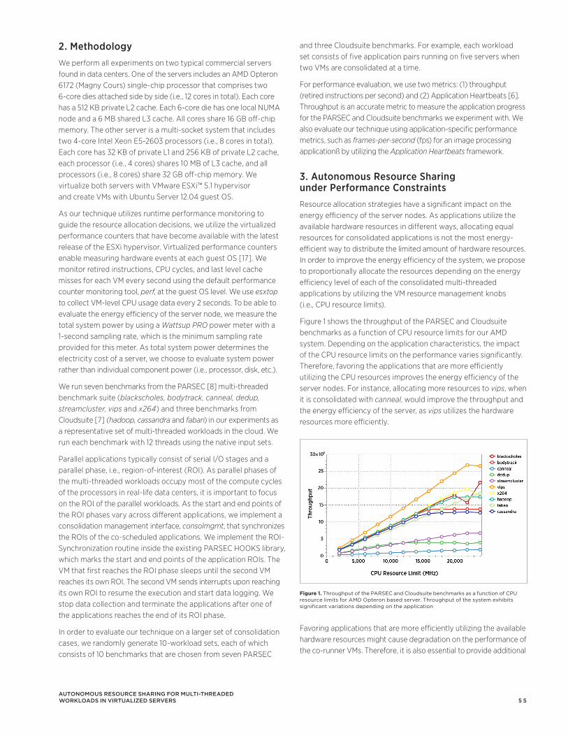
5 5

2. MethodologyWe perform all experiments on two typical commercial servers found in data centers. One of the servers includes an AMD Opteron 6172 (Magny Cours) single-chip processor that comprises two 6-core dies attached side by side (i.e., 12 cores in total). Each core has a 512 KB private L2 cache. Each 6-core die has one local NUMA node and a 6 MB shared L3 cache. All cores share 16 GB off-chip memory. The other server is a multi-socket system that includes two 4-core Intel Xeon E5-2603 processors (i.e., 8 cores in total). Each core has 32 KB of private L1 and 256 KB of private L2 cache, each processor (i.e., 4 cores) shares 10 MB of L3 cache, and all processors (i.e., 8 cores) share 32 GB off-chip memory. We virtualize both servers with VMware ESXi™ 5.1 hypervisor and create VMs with Ubuntu Server 12.04 guest OS.

As our technique utilizes runtime performance monitoring to guide the resource allocation decisions, we utilize the virtualized performance counters that have become available with the latest release of the ESXi hypervisor. Virtualized performance counters enable measuring hardware events at each guest OS [17]. We monitor retired instructions, CPU cycles, and last level cache misses for each VM every second using the default performance counter monitoring tool, perf, at the guest OS level. We use esxtop to collect VM-level CPU usage data every 2 seconds. To be able to evaluate the energy efficiency of the server node, we measure the total system power by using a Wattsup PRO power meter with a 1-second sampling rate, which is the minimum sampling rate provided for this meter. As total system power determines the electricity cost of a server, we choose to evaluate system power rather than individual component power (i.e., processor, disk, etc.).

We run seven benchmarks from the PARSEC [8] multi-threaded benchmark suite (blackscholes, bodytrack, canneal, dedup, streamcluster, vips and x264) and three benchmarks from Cloudsuite [7] (hadoop, cassandra and faban) in our experiments as a representative set of multi-threaded workloads in the cloud. We run each benchmark with 12 threads using the native input sets.

Parallel applications typically consist of serial I/O stages and a parallel phase, i.e., region-of-interest (ROI). As parallel phases of the multi-threaded workloads occupy most of the compute cycles of the processors in real-life data centers, it is important to focus on the ROI of the parallel workloads. As the start and end points of the ROI phases vary across different applications, we implement a consolidation management interface, consolmgmt, that synchronizes the ROIs of the co-scheduled applications. We implement the ROI-Synchronization routine inside the existing PARSEC HOOKS library, which marks the start and end points of the application ROIs. The VM that first reaches the ROI phase sleeps until the second VM reaches its own ROI. The second VM sends interrupts upon reaching its own ROI to resume the execution and start data logging. We stop data collection and terminate the applications after one of the applications reaches the end of its ROI phase.

In order to evaluate our technique on a larger set of consolidation cases, we randomly generate 10-workload sets, each of which consists of 10 benchmarks that are chosen from seven PARSEC

and three Cloudsuite benchmarks. For example, each workload set consists of five application pairs running on five servers when two VMs are consolidated at a time.

For performance evaluation, we use two metrics: (1) throughput (retired instructions per second) and (2) Application Heartbeats [6]. Throughput is an accurate metric to measure the application progress for the PARSEC and Cloudsuite benchmarks we experiment with. We also evaluate our technique using application-specific performance metrics, such as frames-per-second (fps) for an image processing applicationß by utilizing the Application Heartbeats framework.

3. Autonomous Resource Sharing under Performance ConstraintsResource allocation strategies have a significant impact on the energy efficiency of the server nodes. As applications utilize the available hardware resources in different ways, allocating equal resources for consolidated applications is not the most energy-efficient way to distribute the limited amount of hardware resources. In order to improve the energy efficiency of the system, we propose to proportionally allocate the resources depending on the energy efficiency level of each of the consolidated multi-threaded applications by utilizing the VM resource management knobs (i.e., CPU resource limits).

Figure 1 shows the throughput of the PARSEC and Cloudsuite benchmarks as a function of CPU resource limits for our AMD system. Depending on the application characteristics, the impact of the CPU resource limits on the performance varies significantly. Therefore, favoring the applications that are more efficiently utilizing the CPU resources improves the energy efficiency of the server nodes. For instance, allocating more resources to vips, when it is consolidated with canneal, would improve the throughput and the energy efficiency of the server, as vips utilizes the hardware resources more efficiently.

Favoring applications that are more efficiently utilizing the available hardware resources might cause degradation on the performance of the co-runner VMs. Therefore, it is also essential to provide additional


Figure 1. Throughput of the PARSEC and Cloudsuite benchmarks as a function of CPU resource limits for AMD Opteron based server. Throughput of the system exhibits significant variations depending on the application

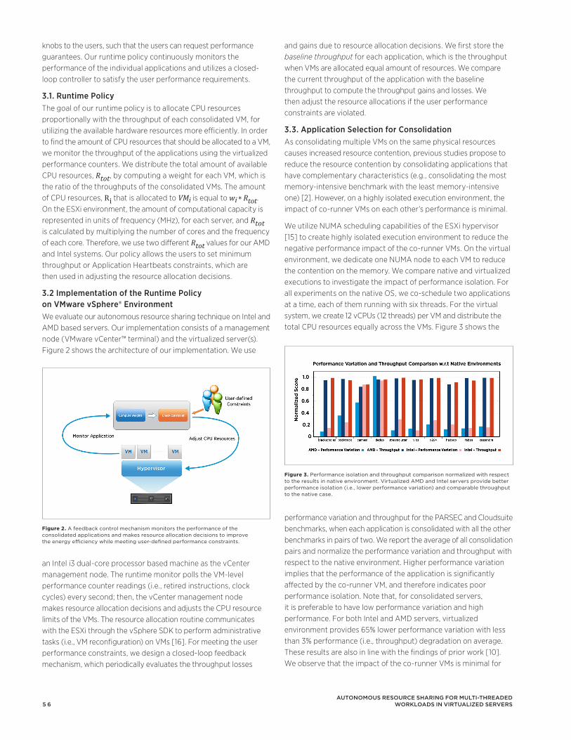
5 6

and gains due to resource allocation decisions. We first store the baseline throughput for each application, which is the throughput when VMs are allocated equal amount of resources. We compare the current throughput of the application with the baseline throughput to compute the throughput gains and losses. We then adjust the resource allocations if the user performance constraints are violated.

3.3. Application Selection for ConsolidationAs consolidating multiple VMs on the same physical resources causes increased resource contention, previous studies propose to reduce the resource contention by consolidating applications that have complementary characteristics (e.g., consolidating the most memory-intensive benchmark with the least memory-intensive one) [2]. However, on a highly isolated execution environment, the impact of co-runner VMs on each other’s performance is minimal.

We utilize NUMA scheduling capabilities of the ESXi hypervisor [15] to create highly isolated execution environment to reduce the negative performance impact of the co-runner VMs. On the virtual environment, we dedicate one NUMA node to each VM to reduce the contention on the memory. We compare native and virtualized executions to investigate the impact of performance isolation. For all experiments on the native OS, we co-schedule two applications at a time, each of them running with six threads. For the virtual system, we create 12 vCPUs (12 threads) per VM and distribute the total CPU resources equally across the VMs. Figure 3 shows the

performance variation and throughput for the PARSEC and Cloudsuite benchmarks, when each application is consolidated with all the other benchmarks in pairs of two. We report the average of all consolidation pairs and normalize the performance variation and throughput with respect to the native environment. Higher performance variation implies that the performance of the application is significantly affected by the co-runner VM, and therefore indicates poor performance isolation. Note that, for consolidated servers, it is preferable to have low performance variation and high performance. For both Intel and AMD servers, virtualized environment provides 65% lower performance variation with less than 3% performance (i.e., throughput) degradation on average. These results are also in line with the findings of prior work [10]. We observe that the impact of the co-runner VMs is minimal for

knobs to the users, such that the users can request performance guarantees. Our runtime policy continuously monitors the performance of the individual applications and utilizes a closed-loop controller to satisfy the user performance requirements.

3.1. Runtime PolicyThe goal of our runtime policy is to allocate CPU resources proportionally with the throughput of each consolidated VM, for utilizing the available hardware resources more efficiently. In order to find the amount of CPU resources that should be allocated to a VM, we monitor the throughput of the applications using the virtualized performance counters. We distribute the total amount of available CPU resources, Rtot, by computing a weight for each VM, which is the ratio of the throughputs of the consolidated VMs. The amount of CPU resources, Ri that is allocated to VMi is equal to wi * Rtot. On the ESXi environment, the amount of computational capacity is represented in units of frequency (MHz), for each server, and Rtot is calculated by multiplying the number of cores and the frequency of each core. Therefore, we use two different Rtot values for our AMD and Intel systems. Our policy allows the users to set minimum throughput or Application Heartbeats constraints, which are then used in adjusting the resource allocation decisions.

3.2 Implementation of the Runtime Policy on VMware vSphere® EnvironmentWe evaluate our autonomous resource sharing technique on Intel and AMD based servers. Our implementation consists of a management node (VMware vCenter™ terminal) and the virtualized server(s). Figure 2 shows the architecture of our implementation. We use

an Intel i3 dual-core processor based machine as the vCenter management node. The runtime monitor polls the VM-level performance counter readings (i.e., retired instructions, clock cycles) every second; then, the vCenter management node makes resource allocation decisions and adjusts the CPU resource limits of the VMs. The resource allocation routine communicates with the ESXi through the vSphere SDK to perform administrative tasks (i.e., VM reconfiguration) on VMs [16]. For meeting the user performance constraints, we design a closed-loop feedback mechanism, which periodically evaluates the throughput losses


Figure 2. A feedback control mechanism monitors the performance of the consolidated applications and makes resource allocation decisions to improve the energy efficiency while meeting user-defined performance constraints.

Figure 3. Performance isolation and throughput comparison normalized with respect to the results in native environment. Virtualized AMD and Intel servers provide better performance isolation (i.e., lower performance variation) and comparable throughput to the native case.

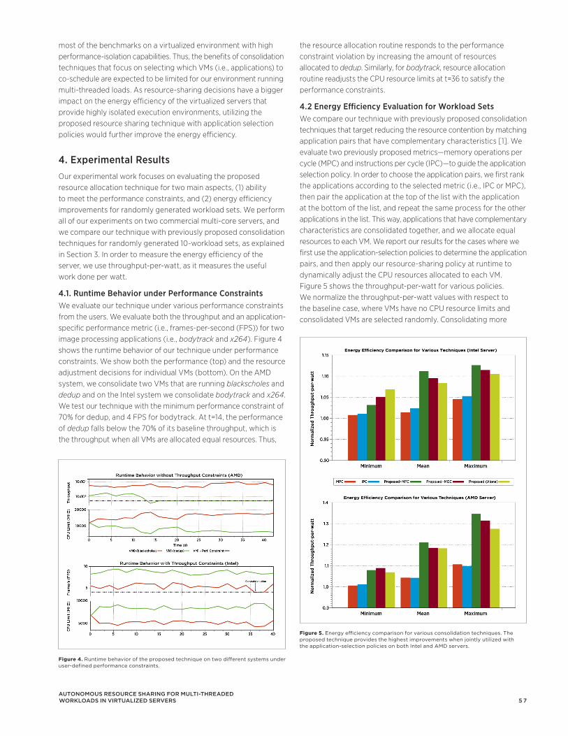
5 7

the resource allocation routine responds to the performance constraint violation by increasing the amount of resources allocated to dedup. Similarly, for bodytrack, resource allocation routine readjusts the CPU resource limits at t=36 to satisfy the performance constraints.

4.2 Energy Efficiency Evaluation for Workload SetsWe compare our technique with previously proposed consolidation techniques that target reducing the resource contention by matching application pairs that have complementary characteristics [1]. We evaluate two previously proposed metrics—memory operations per cycle (MPC) and instructions per cycle (IPC)—to guide the application selection policy. In order to choose the application pairs, we first rank the applications according to the selected metric (i.e., IPC or MPC), then pair the application at the top of the list with the application at the bottom of the list, and repeat the same process for the other applications in the list. This way, applications that have complementary characteristics are consolidated together, and we allocate equal resources to each VM. We report our results for the cases where we first use the application-selection policies to determine the application pairs, and then apply our resource-sharing policy at runtime to dynamically adjust the CPU resources allocated to each VM. Figure 5 shows the throughput-per-watt for various policies. We normalize the throughput-per-watt values with respect to the baseline case, where VMs have no CPU resource limits and consolidated VMs are selected randomly. Consolidating more

most of the benchmarks on a virtualized environment with high performance-isolation capabilities. Thus, the benefits of consolidation techniques that focus on selecting which VMs (i.e., applications) to co-schedule are expected to be limited for our environment running multi-threaded loads. As resource-sharing decisions have a bigger impact on the energy efficiency of the virtualized servers that provide highly isolated execution environments, utilizing the proposed resource sharing technique with application selection policies would further improve the energy efficiency.

4. Experimental ResultsOur experimental work focuses on evaluating the proposed resource allocation technique for two main aspects, (1) ability to meet the performance constraints, and (2) energy efficiency improvements for randomly generated workload sets. We perform all of our experiments on two commercial multi-core servers, and we compare our technique with previously proposed consolidation techniques for randomly generated 10-workload sets, as explained in Section 3. In order to measure the energy efficiency of the server, we use throughput-per-watt, as it measures the useful work done per watt.

4.1. Runtime Behavior under Performance ConstraintsWe evaluate our technique under various performance constraints from the users. We evaluate both the throughput and an application-specific performance metric (i.e., frames-per-second (FPS)) for two image processing applications (i.e., bodytrack and x264). Figure 4 shows the runtime behavior of our technique under performance constraints. We show both the performance (top) and the resource adjustment decisions for individual VMs (bottom). On the AMD system, we consolidate two VMs that are running blackscholes and dedup and on the Intel system we consolidate bodytrack and x264. We test our technique with the minimum performance constraint of 70% for dedup, and 4 FPS for bodytrack. At t=14, the performance of dedup falls below the 70% of its baseline throughput, which is the throughput when all VMs are allocated equal resources. Thus,


Figure 4. Runtime behavior of the proposed technique on two different systems under user-defined performance constraints.

Figure 5. Energy efficiency comparison for various consolidation techniques. The proposed technique provides the highest improvements when jointly utilized with the application-selection policies on both Intel and AMD servers.

5 8

6. Conclusions and Future WorkEnergy efficiency is one of the major challenges for future data centers. The emergence of multi-threaded applications on the cloud resources introduces new challenges for energy-efficient management of hardware resources. In this work, we propose an adaptive solution to energy-efficient management of multi-core servers. The proposed technique takes the energy efficiency of the consolidated applications into account to adjust the amount of CPU resources that are allocated to each VM. We implemented our technique on a vCenter management node and evaluated two commercially available Intel- and AMD-based servers. Our results show that our policy can be jointly utilized with previously proposed consolidation techniques to further improve the energy efficiency by up to 21%.

Open problems in this area include designing scalable management techniques for larger-scale computing clusters, understanding the interference impact of applications from various application domains, and optimizing the performance of power-constrained systems. We plan to extend our work to be more applicable to larger-scale systems by introducing additional capabilities (e.g., VM migration) to our current technique. We also plan to investigate the performance-energy tradeoffs across a wider range of application domains.

References1 G. Dhiman, G. Marchetti, and T. Rosing, “vGreen: A System

for Energy-efficient Computing in Virtualized Environments,” in Proceedings of International Symposium on Low Power Electronics and Design (ISLPED), 2009, pp. 243–248.

2 N. Vasic, D. Novakovic, S. Miucin, D. Kostic, and R. Bianchini, “Dejavu: Accelerating Resource Allocation in Virtualized Environments,” in Architectural Support for Programming Languages and Operating Systems (ASPLOS), 2012, pp. 423–436.

3 M. Bhadauria and S. A. McKee, “An Approach to Resource-aware Co- scheduling for CMPs,” in ACM International Conference on Supercomputing, 2010, pp. 189–199.

4 N. Bobroff, A. Kochut, and K. Beaty, “Dynamic Placement of Virtual Machines for Managing SLA Violations,” in International Symposium on Integrated Network Management, 2007, pp. 119 –128.

5 A. Beloglazov and R. Buyya, “Adaptive Threshold-based Approach for Energy-efficient Consolidation of Virtual Machines in Cloud Data Centers,” in International Workshop on Middleware for Grids, Clouds and e-Science, 2010, pp. 1–6.

than two VMs causes significant performance degradation for multi-threaded applications when compared to running them alone. Therefore, we evaluate our technique for the case where we consolidate two applications at a time, which is a feasible design choice considering the performance requirements.

For randomly generated 10-workload sets, the proposed policy consistently improves the average throughput-per-watt of the system. Utilizing our technique jointly with application-selection policies further improves the energy efficiency. The energy efficiency improvements reach up to 21% for the AMD server and 9% for the Intel server. As the power range, which is the difference between the peak power consumption and the idle power, is much larger on the AMD server, the energy efficiency improvements are significantly higher than the Intel server.

5. Related WorkA number of the existing energy and resource management techniques target optimization of a larger-scale computing cluster (i.e., cluster-level management). Cluster-level resource management techniques can be mainly divided into two groups: VM migration and consolidation techniques. The goal of cluster-level resource management techniques is mainly to provide service availability guarantees and reduce the number of physical servers by turning off the idle nodes (e.g., [4] [5] [14]). VM resource management policies that utilize the history of the VMs to make resource allocation decisions have been also proposed to reduce the overhead of dynamic management [2].

Node-level (i.e., server-level) management techniques provide fine-granularity management for the data centers. Common consolidation techniques at the server level target reducing the resource contention by pairing contrasting applications or threads to work on the same physical resources (e.g., [1]). Application characteristics such as cache misses are utilized to guide the consolidation policies [3]. The success of these techniques relies on the fact that the co-runner VMs affect each other’s performance, which implies poorly isolated execution environment for consolidated VMs. One line of work in consolidation focuses on reducing the impact of interference across consolidated applications [11] [12]. However, the interference impact varies depending on the application domain and the target architecture. In this work, we show that the recent advancements in virtualization technologies provide highly isolated execution environments, which limits the benefits of consolidation techniques for multi-threaded workloads. Our resource sharing technique utilizes multi-threaded application characteristics and guides the resource allocation decisions. In addition, the proposed technique can be utilized together with application-selection policies to further improve the energy efficiency.


5 9

6 H. Hoffmann, S. Sidiroglou, M. Carbin, S. Misailovic, A. Agarwal, and M. Rinard, “Dynamic Knobs for Responsive Power-aware Computing,” in ASLPOS, 2011, pp. 199–212.

7 M. Ferdman, A. Adileh, O. Kocberber, S. Volos, M. Alisafaee, D. Jevdjic, C. Kaynak, A. D. Popescu, A. Ailamaki, and B. Falsafi, “Clearing the Clouds: A Study of Emerging Scale-out Workloads on Modern Hardware,” in International Conference on Architectural Support for Programming Languages and Operating Systems (ASPLOS), 2012, pp. 37–48.

8 C. Bienia, S. Kumar, J. P. Singh, and K. Li, “The PARSEC Benchmark Suite: Characterization and Architectural Implications,” in International Conference on Parallel Architectures and Compilation Techniques (PACT), October 2008.

9 M. Bailey, “The Economics of Virtualization: Moving Toward an Application-Based Cost Model,” International Data Corporation (IDC), Whitepaper, December 2009.

10 J. Kim, M. Ruggiero, D. Atienza Alonso and M. Ledergerber. “Correlation-Aware Virtual Machine Allocation for Energy-Efficient Datacenters,” in IEEE/ACM Design Automation and Test in Europe Conference (DATE), Grenoble, France, March 18-22, 2013.

11 M. Kambadur, T. Moseley, R. Hank, M. A. Kim. “Measuring Interference Between Live Datacenter Applications,” in International Conference on Supercomputing (SC), 2012.

12 Christina Delimitrou and Christos Kozyrakis. “Paragon: QoS-Aware Scheduling for Heterogeneous Datacenters”. In Proceedings of the Eighteenth International Conference on Architectural Support for Programming Languages and Operating Systems (ASPLOS), 2013.

13 L. A. Barroso and U. Holzle, “The Case for Energy-Proportional Computing,” in IEEE Computer, pp. 33–37, 2007.

14 “Resource Management with VMware DRS”, http://vmware.com/pdf/vmware_drs_wp.pdf

15 “vSphere Resource Management”, http://pubs.vmware.com/vsphere-50/topic/com.vmware.ICbase/PDF/vsphere-esxi-vcenter-server-50-resource-management-guide.pdf

16 “vSphere SDK for Perl Documentation”, http://www.vmware.com/support/developer/viperltoolkit/

17 “Using Virtual CPU Performance Monitoring Counters”, http://kb.vmware.com/selfservice/microsites/search.do?language=en_US&cmd=displayKC&externalId=2030221


http://pubs.vmware.com/vsphere-50/topic/com.vmware.ICbase/PDF/vsphere-esxi-vcenter-server-50-resource-management-guide.pdf





VMware Academic Program (VMAP) VMware Academic Program (VMAP)

The VMware Academic Program (VMAP) supports a number of academic research projects across

a range of technical areas. We initiate an annual Request for Proposals (RFP), and also support a

small number of additional projects that address particular areas of interest to VMware.

The 2013 Spring RFP, focused on “Storage in support of Software Defined Datacenters (SDDC)”,

is currently conducting final reviews of a shortlist of proposals and will announce the recipients of

funding at the VMware Research Symposium in July. Please contact Rita Tavilla ([email protected])

if you wish to receive notification of future RFP solicitations and other opportunities for collaboration

with VMware.

The 2012 RFP – Security for Virtualized and Cloud Platforms—awarded funding to three projects:

Timing Side-Channels in Modern Cloud Environments Prof. Michael Reiter, University of North Carolina at Chapel Hill

Random Number Generation in Virtualized Environments Prof. Yevgeniy Dodis, New York University

VULCAN: Automatically Generating Tools for Virtual Machine Introspection using Legacy Binary Code

Prof. Zhiqiang Lin, University of Texas, Dallas

Visit http://labs.vmware.com/academic/rfp find out more about the RFPs.

The VMware Academic Program (VMAP) advances the company’s strategic objectives

through collaborative research and other initiatives. VMAP works in close partnerships with

both the R&D and University Relations teams to engage with the global academic community.

A number of research programs operated by VMAP provide academic partners with

opportunities to connect with VMware. These include:

•AnnualRequestforProposals(seefrontcoverpre-announcement),providingfunding

for a number of academic projects in a particular area of interest.

•ConferenceSponsorship,supportingparticipationofVMwarestaffinacademicconferences

and providing financial support for conferences across a wide variety of technical domains.

•GraduateFellowships,recognizingoutstandingPhDstudentsconductingresearchthat

addresses long-term technical challenges.

•AnnualVMAPResearchSymposium,anopportunityfortheacademiccommunity

to learn more about VMware’s R&D activities and existing collaborative projects.

We also sponsor the VMAP academic licensing program (http://vmware.com/go/vmap),

which provides higher education institutions around the world with access to key VMware

products at no cost to end users.

Visit http://labs.vmware.com/academic/ to learn more about the VMware Academic Program.

VOL. 2, NO. 1–JUNE 2013

VMWARE TECHNICAL JOURNALEditors: Curt Kolovson, Steve Muir, Rita Tavilla

VM

WA

RE

TE

CH

NIC

AL

JOU

RN

AL

VO

L. 2, NO

. 1 2013

VMware, Inc. 3401 Hillview Avenue Palo Alto CA 94304 USA Tel 877-486-9273 Fax 650-427-5001 www.vmware.comCopyright © 2013 VMware, Inc. All rights reserved. This product is protected by U.S. and international copyright and intellectual property laws. VMware products are covered by one or more patents listed at http://www.vmware.com/go/patents. VMware is a registered trademark or trademark of VMware, Inc. in the United States and/or other jurisdictions. All other marks and names mentioned herein may be trademarks of their respective companies. Item No: VMW-TECH-JRNL-VOL2-NO1-COVER-USLET-106TOC

TABLE OF CONTENTS

1 Introduction Steve Muir, Director, VMware Academic Program

2 Memory Overcommitment in the ESX Server Ishan Banerjee, Fei Guo, Kiran Tati, Rajesh Venkatasubramanian

13 Redefining ESXi IO Multipathing in the Flash Era Fei Meng, Li Zhou, Sandeep Uttamchandani, Xiaosong Ma

19 Methodology for Performance Analysis of VMware vSphere under Tier-1 Applications Jeffrey Buell, Daniel Hecht, Jin Heo, Kalyan Saladi, H. Reza Taheri

29 vATM: VMware vSphere Adaptive Task Management Chirag Bhatt, Aalap Desai, Rajit Kambo, Zhichao Li, Erez Zadok

35 An Anomaly Event Correlation Engine: Identifying Root Causes, Bottlenecks, and Black Swans in IT Environments Mazda A. Marvasti, Arnak V. Poghosyan, Ashot N. Harutyunyan, Naira M. Grigoryan

46 Simplifying Virtualization Management with Graph Databases Vijayaraghavan Soundararajan, Lawrence Spracklen

54 Autonomous Resource Sharing for Multi-Threaded Workloads in Virtualized Servers Can Hankendi, Ayse, K. Coskun

We would like to thank all the authors who contributed to this issue. http://labs.vmware.com/academic

vmware technical journaldownload3.vmware.com/software/vmw-tools/papers/vmtj_issue_3.pdf · vol. 2,...

Documents