visualization of output from large-scale brain simulations · visualization of output from...

Available online at www.prace-ri.eu

Partnership for Advanced Computing in Europe

Visualization of output from Large-Scale Brain Simulations

Simon Benjaminssona, David Silverstein

a, Pawel Herman

a,

Paul Melisb, Vladimir Slavnić

c, Marko Spasojević

c, Kiril

Alexievd, Anders Lansner

a,1

aDept of Computational Biology, CSC, KTH Royal institute of Technology bVisualization Group, SARA, Science Park 140, 1098 XG, Amsterdam, The Netherlands

cScientific Computing Laboratory, Institute of Physics Belgrade, University of Belgrade,

Pregrevica 118, 1108, Belgrade, Serbia dDepartment of Mathematical Methods for Sensor Information Processing, Institute of

Information and Communication Technologies, 25A Acad.G.Bonchev Str., Sofia 1113,

Bulgaria

Abstract

This project concerned the development of tools for visualization of output from brain simulations

performed on supercomputers. The project had two main parts: 1) creating visualizations using

large-scale simulation output from existing neural simulation codes, and 2) making extensions to

some of the existing codes to allow interactive runtime (in-situ) visualization. In 1) simulation data

was converted to HDF5 format and split over multiple files. Visualization pipelines were created for

different types of visualizations, e.g. voltage and calcium. In 2) by using the VisIt visualization

application and its libsim library, simulation code was instrumented so that VisIt could access

simulation data directly. The simulation code was instrumented and tested on different clusters

where control of simulation was demonstrated and in-situ visualization of neural unit’s and

population data was achieved.

Project ID: PRPC06

1. Introduction

Today it is possible to simulate very large and also complex brain models on our supercomputers.

The use of such simulations for integrating the massive amounts of experimental data from different

sources and databases is critical for improving our mechanistic understanding of the functions of the

normal and diseased brain and will likely increase dramatically in the near future. Efficient tools for

neural simulation visualization are therefore clearly of interest to the larger computational

neuroscience community. To visualize simulation output in a manner comparable to what can be

obtained experimentally from neuronal as well as macroscopic measurements gives functional

constraints on brain models, which are essential to validate them and for their use to make proper

predictions and propose new critical experiments.

The aim of the project described here was be to develop an HPC workflow and software tools to

1 Corresponding author. E-mail address: [email protected].

Benjaminsson et al. Visualization of output from Large-Scale Brain Simulation / 000–000

2

allow visualization of output from such large-scale neural simulations and to generate animations of

this. This should also be done in real-time by means of “in-situ” visualization, allowing control of

and interaction with a neuronal network while the simulation is running. The simulations

themselves were performed with the widely used NEURON simulator for biophysically detailed

simulations and with a parallelizing simulator developed in-house called BrainCore for more

abstract neuronal networks.

Our main interests have been to visualize changing properties of simulated neural systems and

generate synthetic output. Important properties are neuron membrane potentials, spiking of neurons,

and synaptic strengths between neurons or neural assemblies. More than one property may be of

interest to visualize, either separately or simultaneously. Coordinates of neural elements could be

generated from the simulation and may in some cases be changing over time, as e.g. in axonal

growth. Photorealism has not been an aim. Neuron types could be visualized with different simple

geometrical shapes, e.g. pyramidal cells could be shown as pyramids.

Synthetic “brain imaging” output could be voltage-sensitive dye (VSD), local field potentials (LFP),

and magnetoencephalography (MEG) signals or other output from a simulation that can be directly

related to experimental data. These are not necessarily located at a specific neuron location but are

measured from a region of the brain or a local population of neurons. It could also be an output

based on a specific measure of a simulated population, e.g. a synchrony measure of population

activities or waves of activities. A user should be able to present the information in a specified

geometrical way or mapped in a predefined geometry as specified from a model of a brain or a brain

area, e.g. mapping simulated activity to a whole-brain wireframe model.

The work conducted was divided in three separate parts reflecting those slightly different aims and

approaches, i.e. (i) insight visualization of intracellular potential and calcium levels of single

neurons; (ii) visualization of a neuronal population activity measure (LFP), and (iii) in-situ

(interactive real-time) visualization of network activity. These three parts are described separately

below.

2. Methods

2.1. Neuron data “insight” visualization

One type of visualization done on the simulation datasets are the so-called “insight visualizations”.

These are meant to provide a visual reference of the underlying model’s behavior, to communicate

scientific results, to check model correctness, etc. Important parts of this work were establishing

useful mappings of simulation data to visual primitives and creating practical file layouts. For

creating the insight visualizations we used ParaView 3.12 [1]. This is a widely used open-source

scientific visualization package that provides flexible visualization functionality based on a pipeline

model. It also provides parallel rendering, which is of interest for visualization of future large-scale

brain models.

Specifications of the PC system used for producing the visualizations in this section are: Ubuntu

Linux x86_64 system, Intel Core i7 @ 3.4 GHz, NVidia Geforce GTX 560 Ti. The system also had

a 160 GByte solid-state disk, which most likely positively influenced the rendering performance,

since reading data during rendering is a lot faster from a SSD than when using a conventional

spinning hard-drive.


3

2.1.1. Model description

The model of a neocortical patch with neural spiking visualization was partially based on an

attentional blink simulation done previously [1]. The simulation replicates the Rapid Visual Serial

Presentation (RVSP) paradigm where visual items are presented in a serial stream and subjects are

told to attend to particular items. The model consisted of two brain regions, a lower patch represents

the parietal cortex and a higher patch represents the dorsal lateral prefrontal cortex (DLPFC). In

total, the model had 55,296 neurons, divided evenly between the two regions. Each region is a patch

of 4x4 hypercolumns, each containing 64 minicolumns. Each hypercolumn has 128 basket cells and

each minicolumn has 5 layer-4 pyramidal cells and 20 layer-2/3 pyramidal cells. 64 orthogonal

memory patterns are stored in each region as long-range connections between minicolumns. There

are both feed-forward and feed-back projections between the regions which represent activity in the

superior longitudinal fasciculus. This model does not have a visual cortex, so the parietal network is

activated directly.

The network model was implemented such that it can be scaled to much larger sizes. It was

successfully scaled up computationally on IBM Blue Gene supercomputers, although a 3D

visualization of the output was not done at this time. The simulations ran for 1 second of cortical

activity and stimulated a single memory pattern for attractor activation and pattern completion. On

the Blue Gene/L at PDC, two cortical patches with feedforward projections similar to the visualized

attentional blink model were scaled up to 32x32 hypercolumns with 128 minicolumns per

hypercolumn. The model had 7 million neurons connected with 960 million synapses and executed

on 2048 cores for 3 hours. On jugene, a Blue Gene/P at Julich, a single cortical patch was scaled up

to 128x128 hypercolumns with 128 minicolumns per hypercolumn. This model had 57 million

neurons connected with 7 billion synapses and executed on 16,384 cores for 3 hours and 20

minutes.

In the simulation protocol, a single unpotentiated memory pattern is stimulated at 100 ms into the

simulation, for a duration of 60 ms. Following this starting at 1000 ms a sequence of 15 memory

patterns are stimulated for 60 ms. Two of these are potentiated by 0.75 mV and the rest

hyperpolarized by 0.75 mV. To activate a memory pattern in the parietal network, layer 4 pyramidal

cells are stimulated in 5 of 16 minicolumns. This stimulation activates layer 2/3 pyramidals in those

minicolumns, which are recurrently connected locally within the minicolumns and globally across

hypercolumns of the region. If the activity is high enough, a pattern will complete across all

minicolumns of the memory pattern. Active minicolumns within the parietal network also stimulate

memory patterns within the DLPFC network, via the feedforward projections and provide pattern

recurrence via the feedback projections. When an item in the RSVP stream is selected to be

attended, the corresponding memory pattern in the DLPFC network is potentiated. If the attractor

memory activation in the parietal network is high enough, a corresponding memory pattern will

become active in the DLPFC as well, which in turn provides more recurrent activation in the

parietal network. The model represents an attentional gate, so if a distributed memory pattern

becomes active across both regions, this would represent awareness of a presented item.

To create the model neural coordinates, synapses and projections, a Matlab program was used to

generate brain regions, hypercolmns, minicolumns, neuron coordinates, neuron rotations and inter-

region projections. In each patch region, neurons were placed in space by generating planes for the

minicolumns and basket cells. Minicolumn positions were placed randomly within hypercolumns,

with a minimum distance. Basket cells were placed between these, with minimum distances

between the minicolumn positions and themselves. At each minicolumn coordinate, pyramidal cells


4

were placed at different z positions, separated by fixed distance. A small amount of noise was also

added to the neural coordinates within the minicolumn. For each region, neuron numbers, types,

coordinates and rotations were written to an ascii file, which was then converted to an HDF5 file

(neurons.hdf5, see 2.1.2) with a python program. Feedforward projections were from single

minicolumns to single minicolumns, between the corresponding memory patterns in each region.

Feedback projections were from single minicolumns in the source region to the six closest

minicolumns in the destination region.

The attentional blink simulations were run on 256 cores on an IBM Blue Gene/L, using the Parallel

NEURON simulator. Within the Hodgkin-Huxley neurons, soma voltage membrane potentials and

calcium concentrations were captured in 5 ms intervals. These were written out to files, which were

also used for the visualizations. Each core was assigned two minicolumns, with one from the

parietal region (lower patch) and one from the DLPFC region (upper patch). On each core, recorded

output for soma membrane potentials or calcium concentrations was written to a separate ascii file

in 5 ms intervals and included time, neuron number, neuron type and measured value. To convert

this output to HDF5 files, several steps were needed. After all the individual core-specific files

were concatenated together into one large file, the file was sorted first by simulation time and then

by cell number. After this, A python program would step through each visualization time-step, read

all neurons with measured values and write this out as a neuron-indexed vector in a single HDF5

file (volts.hdf5 or somaca.hdf5, see 2.1.2) for each time-step. This program was file-based, in order

to avoid being memory bound and thus be able to scale to large network sizes. However, it was

rather slow, since searching for each time-step was done serially. This can be greatly improved in

the future by seeking forward in the file for each time-step a determinable number of fixed lines.

To visualize activity between regions, a projection activity file was generated, using another Matlab

program. Projections between regions were originally generated from source and destination

minicolumns. Spiking activity was also saved during simulations as events, with time and neuron

number. So, to generate projection activity between regions, spiking activity was aggregated by

minicolumn within a 50 ms sliding time window. If spikes occurred in a minicolumn within a

current time window, activity was written out between active source minicolumns and destination

minicolumns, based on the minicolumn to minicolumn projections. The format of the projection

activity file was the activity timestep in 50 ms intervals, number of spikes in the source minicolumn

and x,y,z coordinates of the source and destination minicolumns. The projection activity file was

read in during visualization to show projection activity over a straight line. Future work can include

replacing this line with a spline derived from diffusion tensor imaging of white-matter data between

connected regions of interest. It might also include showing feedforward and feedback activity in

different colors to show recurrent activity between regions.

2.1.2. Data organization

As described above, the simulation writes its output in a number of custom text-based file formats.

These formats cannot be read directly by ParaView, so either the simulator code needed to be

changed to write to a more appropriate file format, or the current output files needed to be converted

in a post-processing step. The latter approach was chosen, since it involved less work. In future, the

MPI-based simulator code might be augmented to directly produce data in the necessary file

formats.

Simulation data was converted to Xdmf format ([3]), which uses a combination of storing large-

scale data arrays in HDF5 files, while associated metadata is stored in a separate XML file. The


5

Xdmf format can store datasets with different topologies (e.g. unstructured and structured grids and

general geometric data). It allows per-element data attributes and has support for storing time series

and hierarchical datasets. Most interestingly, ParaView has built-in support for reading Xdmf files.

As mentioned, the actual simulation output was converted to HDF5 files, thereby providing

efficient data containers that can fairly easily be read and written by custom tools, based on the

HDF5 library.

A fairly straightforward data layout for the HDF5 files was used. As certain per-neuron values don't

change over time, like position, we store them in a single HDF5 file called "neurons.hdf5", which

has the following data layout:

HDF5 "neurons.hdf5" {

GROUP "/" {

DATASET "neurontype" {

DATATYPE H5T_STD_I8LE

DATASPACE SIMPLE { ( 55296, 1 ) / ( 55296, 1 ) }

}

DATASET "position" {

DATATYPE H5T_IEEE_F32LE


}

DATASET "rotation" {



}

}

}

As can be seen each neuron has a fixed 3D position and orientation (expressed as a rotation from a

base orientation). Different types of neurons are distinguished by single integer type field (1 = layer

4 pyramidal, 2 = layer 2/3 pyramidal, 3 = basket).

The time-varying model data was stored in separate HDF5 files, one for each timestep, containing

the voltages for all the neurons:

HDF5 "volts_0000ms.hdf5" {

GROUP "/" {

ATTRIBUTE "measurement" {

DATATYPE H5T_STRING {

STRSIZE 4;

STRPAD H5T_STR_NULLPAD;

CSET H5T_CSET_ASCII;

CTYPE H5T_C_S1;

}

DATASPACE SCALAR

}

ATTRIBUTE "microsec" {

DATATYPE H5T_STD_I32LE

DATASPACE SCALAR

}


6

DATASET "voltage" {



}

}

}

Time-varying calcium concentrations were stored using a similar layout.

Spiking neurons were detected by processing the voltage series and thresholding the voltage values.

In general, there are far fewer spikes than there are timesteps. The spikes were stored as a simple

position/rotation pair, allowing spikes to be highlighted by placing a visual marker in the relevant

position:

HDF5 "spikes_0080ms.hdf5" {

GROUP "/" {

DATASET "spike_positions" {



DATA {

(0,0): 0.00127422, 0.000228367, 0.00115082

}

}

DATASET "spike_rotations" {



DATA {

(0,0): -0.240513, -0.260281, -0.0988702

}

}

}

}

A small number of Xdmf files were created that combined a series of per-timestep HDF5 files with

the fixed attributes in the neuron data file.

2.1.3. Visualizations

Abstract visualizations of the simulation data were produced, based on the Xdmf datasets described

in the previous section. The neurons themselves were visualized using “glyphs” – small abstract

visual elements placed at the neuron positions. Here, we chose simple points, each a few pixels

wide. The glyphs are colored by membrane potential (voltage in millivolts). For spiking neurons,

whose voltage exceeds a certain threshold, larger cone-shaped glyphs are shown. These cones are

also oriented based on the neuron rotation values.

Projections

Activity over the forward projections between the two areas of neurons was visualized by animating

a series of glyphs between the sending and receiving minicolumns. For each projection event a


7

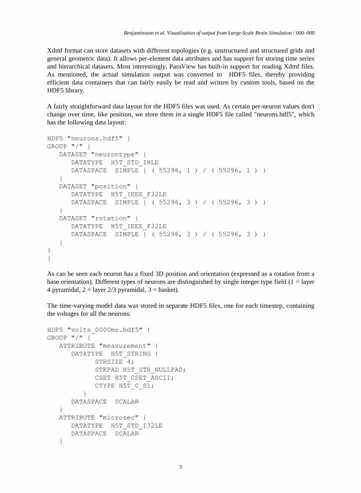
varying number of potential spikes travel between the minicolumns in a 50 ms interval. Each spike

is represented by a sphere glyph, its size relative to the number of spikes in the interval. In

Figure 1, one frame of the visualization is shown, 140 ms into the lag5 simulation. Also visible are

the oriented spiking glyphs, colored by soma membranevoltage potential.

Figure 1

Wireframe brain

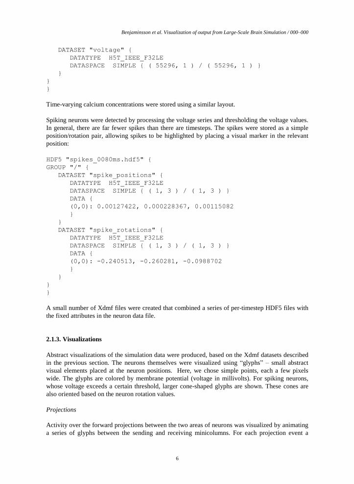
A wireframe model of a brain was added to provide some spatial context for the simulation model

(Figure 2). The basis for this model was a publicly available MRI dataset, from which an isosurface

was extracted, followed by decimating the resulting mesh.

The placement of the simulation model within the brain is currently done visually, based on the

average location of the parietal cortex within the brain. In future, proper placement based on e.g.

Talairach coordinates might be used.

Figure 2

Calcium imaging


8

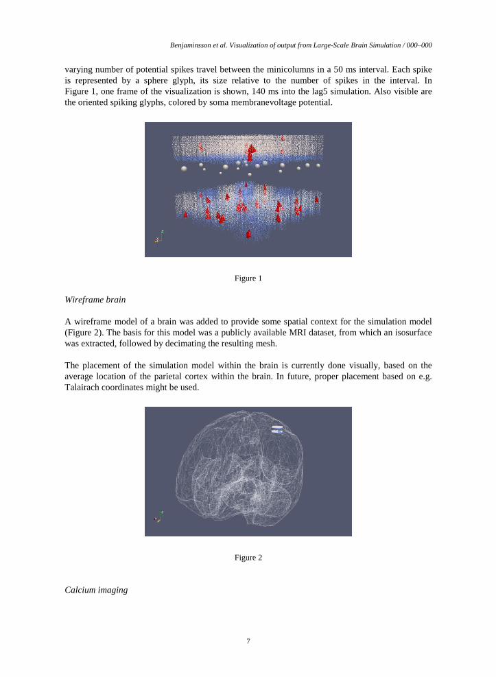
A separate variant of the above visualisations was made for the case of calcium imaging. Instead of

membrane potentials, per-neuron soma calcium soma concentrations were produced by the

simulation. The visualization pipeline used for calcium imaging largely corresponds to the pipeline

used for the membrane potential visualizations. Small changes were the use of grey-to-white color

mapping of calcium concentrations and the use of a black background. This color scheme matches

real-life calcium imaging results.

Figure 3

2.2. In-situ visualization of neural dynamics

Today’s scientific simulations are often distributed over many thousands of cores,producing large

amounts of data which are written to hard disks. As the access time of disk drives is several orders

of magnitude higher than CPU-to-memory access, writing results to disk files creates a major

performance bottleneck. Common usage of visualization tools imply that users import their data via

disk files, making data visualization and analysis a post-processing step. In-situ visualization

addresses this problem by giving users an opportunity to visualize their data while the simulation is

running, by gaining direct access to the memory pointers of the simulation code and providing the

ability to steer the execution of the simulation (stop, reset, continue to run). In addition to this

approach, visualization of the data uses the same level of resources that are being used for data

generation. Usually, visualization receives fewer processing resources, typically only a local

computer.

VisIt [4] is a free, open source, platform independent, distributed, parallel tool for visualizing and

analyzing large scale simulated and experimental data sets. Target use cases include data

exploration, comparative analysis, visual debugging, quantitative analysis, and presentation

graphics. VisIt employs a distributed and parallel architecture in order to handle extremely large

data sets interactively. An important additional feature is its in-situ approach which is provided by

its libsim library, which allows the visualization of simulation data in situ, thus avoiding the high

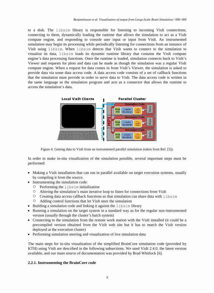
costs of I/O associated with first writing and then reading the same data again (Figure 4). The

libsim simulation instrumentation library can be inserted into a simulation program to make the

simulation act in many ways like a VisIt compute engine (component that reads the data and

performs most of VisIt’s processing). This library, coupled with some additional data access code

that has to be written by the user and built into the simulation, gives to VisIt’s data processing

routines access to the simulation’s calculated data without the need for the simulation to write files

Figure 3


9

to a disk. The libsim library is responsible for listening to incoming VisIt connections,

connecting to them, dynamically loading the runtime that allows the simulation to act as a VisIt

compute engine, and responding to console user input or input from VisIt. An instrumented

simulation may begin its processing while periodically listening for connections from an instance of

VisIt using libsim. When libsim detects that VisIt wants to connect to the simulation to

visualize its data, libsim loads its dynamic runtime library that contains the VisIt compute

engine’s data processing functions. Once the runtime is loaded, simulation connects back to VisIt’s

Viewer and requests for plots and data can be made as though the simulation was a regular VisIt

compute engine. When a request for data comes in from VisIt’s Viewer, the simulation is asked to

provide data via some data access code. A data access code consists of a set of callback functions

that the simulation must provide in order to serve data to VisIt. The data access code is written in

the same language as the simulation program and acts as a connector that allows the runtime to

access the simulation’s data.

Figure 4. Getting data to VisIt from an instrumented parallel simulation (taken from Ref. [5]).

In order to make in-situ visualization of the simulation possible, several important steps must be

performed:

Making a VisIt installation that can run in parallel available on target execution systems, usually

by compiling it from the source.

Instrumenting the simulation code:

○ Performing the libsim initialization

○ Altering the simulation’s main iterative loop to listen for connections from VisIt

○ Creating data access callback functions so that simulation can share data with libsim

○ Adding control functions that let VisIt steer the simulation

Building a simulation code and linking it against the libsim library

Running a simulation on the target system in a standard way as for the regular non-instrumented

version (usually through the cluster’s batch system)

Connecting to the simulation from the remote work station with the VisIt installed (it could be a

precompiled version obtained from the VisIt web site but it has to match the VisIt version

deployed at the execution cluster)

Performing simulation steering and visualization of live simulation data

.

The main steps for in-situ visualization of the simplified BrainCore simulation code (provided by

KTH) using VisIt are described in the following subsections. We used VisIt 2.4.0, the latest version

available, and our main source of documentation was provided by Brad Whitlock [6].

2.2.1. Instrumenting the BrainCore code


10

The BrainCore code is object-oriented C++ code for neural simulations which uses the Message

Passing Interface (MPI) for parallelization. It has been shown to have good scaling properties up to

hundred thousands of cores [7]. The main part of the code base is a library that implements the

simulation and provides ability for a user to configure the network and simulation process. The

remaining part consists of examples of using the network library in which simple network structures

and simulations are defined. We used one example network for libsim instrumentation.

We performed the initialization of the VisIt environment in the main() function and in the

constructor of the class NetworkDemoVis which is derived from the Network class. Changes in

the main()function included adding the VisIt initialization function

VisItSetupEnvironment() and changes in the constructor included registering the callback

functions for global communication:

VisItSetBroadcastIntFunction(visit_broadcast_int_callback);

VisItSetBroadcastStringFunction(visit_broadcast_string_callback);

calling functions that set libsim to operate in parallel and set the rank of the current process

within its MPI communicator:

VisItSetParallel(sim.par_size > 1);

VisItSetParallelRank(sim.par_rank);

and finally adding the function VisItInitializeSocketAndDumpSimFile(), that will be

executed only by the process with rank 0 and which makes simulation start listening for inbound

VisIt socket connections and writes a .sim2 file that tells VisIt client how to connect to the

simulation.

We added the simulation_data type field to the class NetworkDemoVis. This is a structure

which consists of fields that represent the simulation state (process rank, the number of processes,

simulation cycle…). NetworkRun() method, the member of the example NetworkDemoVis

class, redefines the virtual method in the base class Network. This method was used as a

simulation mainloop function (typical libsim in-situ approach), where all interactions with VisIt

were defined and through which single steps of simulation were called (Simulate() method of

Network class). Function VisItDetectInput() was added to detect the VisIt client input

from the listen socket and switch block in which different actions were defined, depending on the

output of the VisItDetectInput()function: To continue with the simulation (simulate one

step) if there is no VisIt input, to try to successfully connect to VisIt if that kind of attempt was

detected, to respond to VisIt’s request to perform a particular compute engine command, and finally

to detect an error in VisIt interaction. It is important to say that only the root MPI process (with rank

0) performs execution of VisItDetectInput() function and it broadcasts its output to all other

MPI instances. In case of successful connection with remote VisIt client, functions that forward

metadata to client and perform registering of functions for accessing the mesh and variables data are

executed:

VisItSetCommandCallback(ControlCommandCallback, (void*)sim);

VisItSetSlaveProcessCallback(SlaveProcessCallback);

VisItSetGetMetaData(SimGetMetaData, (void*)sim);

VisItSetGetMesh(SimGetMesh,(void*)sim);

VisItSetGetVariable(SimGetVariable, (void*)sim);


11

The first function registers the ControlCommandCallback() function, which allows steering

of the simulation through VisIt simulations window and Commands buttons from the Controls tab

(like stopping the simulation, running the simulation, updating the plots, etc.).

VisItSetSlaveProcessCallback()sets the callback function used to inform slave

processes that they should call VisItProcessEngineCommand().

We described the 2D mesh and variables in the SimGetMetadata()callback function. In this

function we called VisIt functions with prefixes VisIt_MeshMetaData and

VisIt_VariableMetaData which allows defining the mesh and variable properties (name,

type, units, labels, etc.).

In the callback function SimGetMesh() we have provided the arrays which define the rectilinear

mesh. The rectilinear mesh is described before the entry in the mainloop in the NetworkRun()

method. It was important to divide the mesh among processes so that each process generates data

for the one part of the mesh. The rows of the rectilinear mesh represent the hypercolumns, and

columns of the mesh represent the minicolumns.

In the callback function SimGetVariable() we provided the array which is populated by the

simulation process. This variable is attached to the described mesh, and every cell of the mesh is

populated by the value of the corresponding minicolumn. The array is populated in every simulation

step.

The BrainCore simulation code is linked statically against the libsim library (libsimV2.a). In

addition to this, there is also a runtime library (libsimV2runtime_par.so) which is loaded

after the successful connection of VisIt client to the running simulation. We used the version V2 of

the libsim which is a newer and more advanced version and successor to the version V1.

2.2.2. Executing and connecting to the instrumented simulation

For initial development we have used the PARADOX Cluster at the Scientific Computing

Laboratory of the Institute of Physics Belgrade, and later, for actual tests and visualization of live

simulation data of the simplified BrainCore code, we have used the Linux Cluster PLX [8] provided

by CINECA, Italy. It is an IBM iDataPlex DX360M3 made of 274 compute nodes, each containing

2 NVIDIA® Tesla® M2070 and 2 Intel(R) Xeon(R) Westmere six-core E5645 processors. In

addition, it has 6 RVN nodes for pre- and post-processing activities, supporting DCV-RVN remote

visualization software of IBM. The connection to a running simulation was performed in two ways:

Using a remote workstation (a laptop or a desktop machine) outside of CINECA, starting VisIt

client locally and connecting through the PLX login node (default machine for submitting jobs

and interacting with the PLX cluster) to running BrainCore simulation. This is a common way

for users to connect to the simulation and use in-situ visualization.

Using local PLX RVN nodes, by establishing a VNC client/server connection with the RVN

node, starting VisIt client and connecting to the running simulation.

Simulations were started on the PLX Cluster by using standard job submission using the available

PBS scheduler. In order for a simulation to load the VisIt runtime environment, a visit command

was added to the user’s PATH at the PLX cluster.

In order to connect to a running simulation, a user needs to start a VisIt client, define a host profile

for the PLX login node with SSH tunneling option checked (host profiles definition is very useful


12

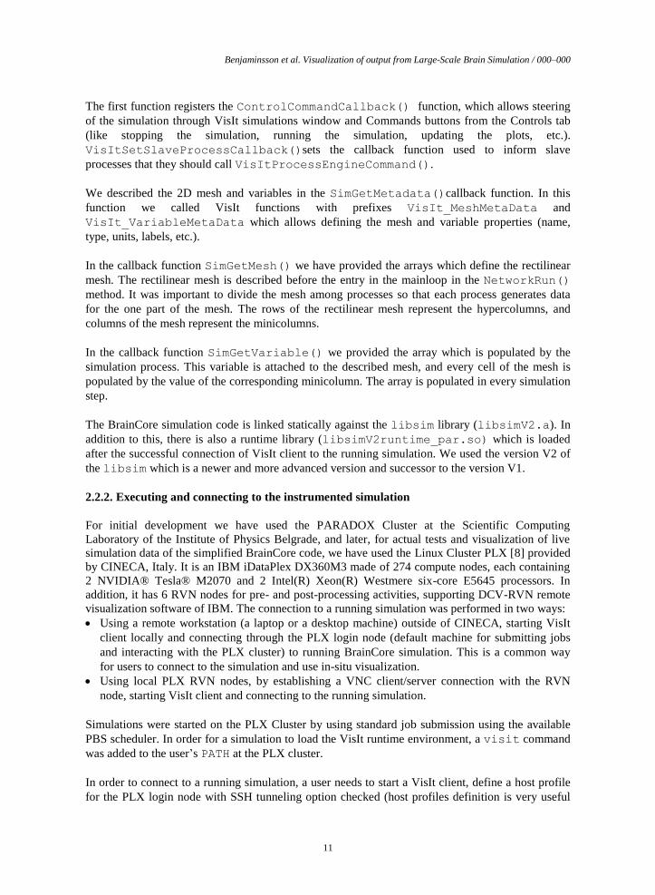
feature of VisIt tool), perform a standard file open by choosing the PLX login node for the host,

navigate to $HOME/.visit/simulations directory and select the appropriate .sim2 file

created by the running simulation (Figure 5). When RVN nodes with VNC connection are used it is

only necessary to open simulation the .sim2 file from the localhost because RVN nodes are

sharing the user’s $HOME directory (location of .visit/simulations directory) with other

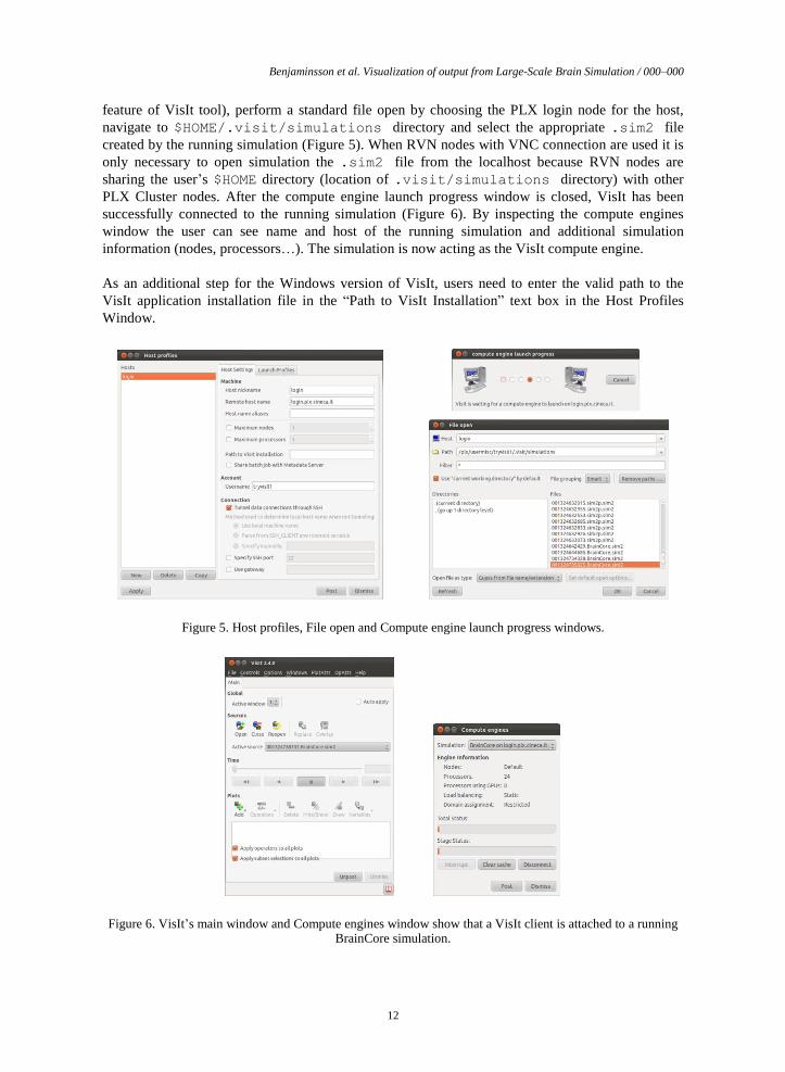
PLX Cluster nodes. After the compute engine launch progress window is closed, VisIt has been

successfully connected to the running simulation (Figure 6). By inspecting the compute engines

window the user can see name and host of the running simulation and additional simulation

information (nodes, processors…). The simulation is now acting as the VisIt compute engine.

As an additional step for the Windows version of VisIt, users need to enter the valid path to the

VisIt application installation file in the “Path to VisIt Installation” text box in the Host Profiles

Window.

Figure 5. Host profiles, File open and Compute engine launch progress windows.

Figure 6. VisIt’s main window and Compute engines window show that a VisIt client is attached to a running BrainCore simulation.


13

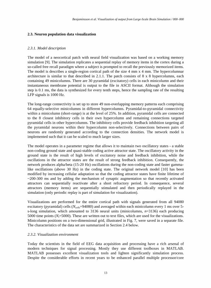
2.3. Neuron population data visualization

2.3.1. Model description

The model of a neocortical patch with neural field visualization was based on a working memory

simulation [9]. The simulation replicates a sequential replay of memory items in the cortex during a

so-called free recall paradigm where a subject is prompted to recall the previously memorized items.

The model is describes a single-region cortical path of the size 4 mm x 4 mm. The hypercolumnar

architecture is similar to that described in 2.1.1. The patch consists of 8 x 8 hypercolumns, each

containing 49 minicolumns. There are 30 pyramidal (excitatory) cells in each minicolumn and their

instantaneous membrane potential is output to the file in ASCII format. Although the simulation

step is 0.1 ms, the data is synthesized for every tenth steps, hence the sampling rate of the resulting

LFP signals is 1000 Hz.

The long-range connectivity is set up to store 49 non-overlapping memory patterns each comprising

64 equally-selective minicolumns in different hypercolumns. Pyramidal-to-pyramidal connectivity

within a minicolumn (short-range) is at the level of 25%. In addition, pyramidal cells are connected

to the 8 closest inhibitory cells in their own hypercolumn and remaining connections targeted

pyramidal cells in other hypercolumns. The inhibitory cells provide feedback inhibition targeting all

the pyramidal neurons within their hypercolumn non-selectively. Connections between pairs of

neurons are randomly generated according to the connection densities. The network model is

implemented such that it can be scaled to much larger sizes.

The model operates in a parameter regime that allows it to maintain two oscillatory states - a stable

non-coding ground state and quasi-stable coding active attractor state. The oscillatory activity in the

ground state is the result of high levels of excitatory noise and feedback inhibition, while the

oscillations in the attractor states are the result of strong feedback inhibition. Consequently, the

network produces alpha/beta (15-20 Hz) oscillations during the non-coding state and faster gamma-

like oscillations (above 30 Hz) in the coding state. The original network model [10] has been

modified by increasing cellular adaptation so that the coding attractor states have finite lifetime of

~200-300 ms and by adding the mechanism of synaptic augmentation so that recently activated

attractors can sequentially reactivate after a short refractory period. In consequence, several

attractors (memory items) are sequentially stimulated and then periodically replayed in the

simulation (only periodic replay is part of simulation for visualization).

Visualizations are performed for the entire cortical path with signals generated from all 94080

excitatory (pyramidal) cells (Ncells=94080) and averaged within each minicolumn every 1 ms over 5-

s-long simulation, which amounted to 3136 neural units (minicolumns, n=3136) each producing

5000 time points (Nt=5000). These are written out to text files, which are used for the visualizations.

Minicolumn positions on a two-dimensional grid, illustrated in Fig. 7, were saved in a separate file.

The characteristics of the data set are summarized in Section 2.4 below.

2.3.2. Visualization environment

Today the scientists in the field of EEG data acquisition and processing have a rich arsenal of

modern techniques for signal processing. Mostly they use different toolboxes in MATLAB.

MATLAB possesses excellent visualization tools and lighten significantly simulation process.

Despite the considerable efforts in recent years to be enhanced parallel multiple processor/core


14

computations and GPU computations, MATLAB still remains a tool for modeling and simulation of

systems with limited amounts of data. That is why we choose another tool for visualization,

developed by Lawrence Livermore National Laboratory. VisIt [4] is a free, open source, platform

independent, distributed, parallel visualization tool. It uses data defined on two- and three-

dimensional structured and unstructured meshes. VisIt’s distributed architecture allows it to explore

both the computational power of a large parallel computer and the graphics acceleration hardware of

a local workstation.

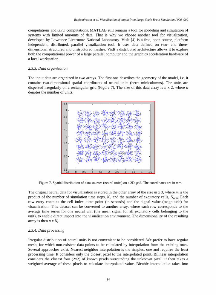
2.3.3. Data organization

The input data are organized in two arrays. The first one describes the geometry of the model, i.e. it

contains two-dimensional spatial coordinates of neural units (here: minicolumns). The units are

dispersed irregularly on a rectangular grid (Figure 7). The size of this data array is n x 2, where n

denotes the number of units.

Figure 7. Spatial distribution of data sources (neural units) on a 2D grid. The coordinates are in mm.

The original neural data for visualization is stored in the other array of the size m x 3, where m is the

product of the number of simulation time steps, Nt, and the number of excitatory cells, Ncells. Each

row entry contains the cell index, time point (in seconds) and the signal value (magnitude) for

visualization. This dataset can be converted to another array, where each row corresponds to the

average time series for one neural unit (the mean signal for all excitatory cells belonging to the

unit), to enable direct import into the visualization environment. The dimensionality of the resulting

array is then n x Nt.

2.3.4. Data processing

Irregular distribution of neural units is not convenient to be considered. We prefer to have regular

mesh, for which non-existent data points to be calculated by interpolation from the existing ones.

Several approaches exist. Nearest neighbor interpolation is the simplest one and requires the least

processing time. It considers only the closest pixel to the interpolated point. Bilinear interpolation

considers the closest four (2x2) of known pixels surrounding the unknown pixel. It then takes a

weighted average of these pixels to calculate interpolated value. Bicubic interpolation takes into


15

account the closest 16 (4x4) known pixels, while higher order interpolation applies spline, sinc or

other functions for interpolation. These algorithms require considerable more computational

resources).

3. Results

3.1. Neuron data visualization

The glyph visualizations of the simulation model nicely provide a visual confirmation that the

organization of neurons into mini-columns, hyper-columns and areas is correct. Furthermore, the

spreading of activity throughout the network can be verified with the projections and inspected one

visualization timestep at a time.

The interactive visualisation of the model in ParaView works well, as the number of neurons isn’t

that large in the simulation runs performed so far . The current model can be easily rendered in

ParaView on a standard workstation with graphics card. When animating the simulation,

visualization timesteps can be displayed fairly quickly in succession.

Using the Xdmf format for data storage worked reasonably well. The only reference to the format is

a short document describing the XML structure and a bit of trial-and-error was sometimes needed to

get data successfully loaded in ParaView. We unfortunately stumbled upon a number of crasher

bugs and other incorrect functionality in ParaView 3.12 during this project, most of which has been

reported to the ParaView bug tracker website and hopefully will get fixed in the near future.

Another issue with ParaView is the difficulty of creating a reusable visualization pipeline that can

serve as a template for visualizing multiple input datasets. The most attractive way of working with

ParaView is to load one or more datasets and interactively piece together a visualization pipeline

that produces a satisfactory visualization. In this workflow, changes to the pipeline lead to

immediate visual feedback. Once a pipeline is deemed satisfactory one would like to reuse it with

different input data, but this proves a bit cumbersome, as changing input data needs to be done

manually followed by saving the updated pipeline to a new file. Having a pipeline template in which

the input datasets are a parameter would be a much more workable approach. Although Python

scripting is available in ParaView for programmatically creating pipelines, this way of working

lacks the interactive feedback. A “Python tracing mode” is available that basically records pipeline

edits to a Python script, but the resulting scripts didn’t always correctly reproduce the pipelines.

Another option, saving a finished pipeline to a Python script, had the same problems.

3.2. In-situ visualization

We successfully implemented an in-situ visualization approach to a simplified version of BrainCore

and demonstrated a simple and convenient way of using this type of visualization in general: from

code instrumentation to live data visualization.

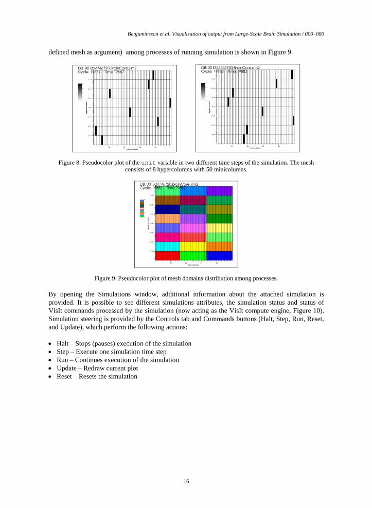
After successful connection to a BrainCore simulation running on the PLX Cluster (see 2.2.2), it is

possible to investigate data and make plots. By adding a standard VisIt pseudocolor plot and

choosing the unit variable the user can see the neural activity in the current simulation time step

(Figure 8). Each row of the plot represents one hypercolumn and each cell in the row represents one

minicolumn. VisIt’s mesh distribution (result of expression which calls VisIt’s procid function on


16

defined mesh as argument) among processes of running simulation is shown in Figure 9.

Figure 8. Pseudocolor plot of the unit variable in two different time steps of the simulation. The mesh consists of 8 hypercolumns with 50 minicolumns.

Figure 9. Pseudocolor plot of mesh domains distribution among processes.

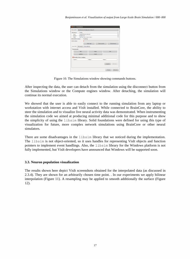
By opening the Simulations window, additional information about the attached simulation is

provided. It is possible to see different simulations attributes, the simulation status and status of

VisIt commands processed by the simulation (now acting as the VisIt compute engine, Figure 10).

Simulation steering is provided by the Controls tab and Commands buttons (Halt, Step, Run, Reset,

and Update), which perform the following actions:

Halt – Stops (pauses) execution of the simulation

Step – Execute one simulation time step

Run – Continues execution of the simulation

Update – Redraw current plot

Reset – Resets the simulation


17

Figure 10. The Simulations window showing commands buttons.

After inspecting the data, the user can detach from the simulation using the disconnect button from

the Simulations window or the Compute engines window. After detaching, the simulation will

continue its normal execution.

We showed that the user is able to easily connect to the running simulation from any laptop or

workstation with internet access and VisIt installed. While connected to BrainCore, the ability to

steer the simulation and to visualize live neural activity data was demonstrated. When instrumenting

the simulation code we aimed at producing minimal additional code for this purpose and to show

the simplicity of using the libsim library. Solid foundations were defined for using this type of

visualization for future, more complex network simulations using BrainCore or other neural

simulators.

There are some disadvantages in the libsim library that we noticed during the implementation.

The libsim is not object-oriented, so it uses handles for representing VisIt objects and function

pointers to implement event handlings. Also, the libsim library for the Windows platform is not

fully implemented, but VisIt developers have announced that Windows will be supported soon.

3.3. Neuron population visualization

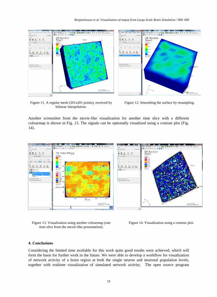
The results shown here depict VisIt screenshots obtained for the interpolated data (as discussed in

2.3.4). They are shown for an arbitrarily chosen time point. . In our experiments we apply bilinear

interpolation (Figure 11). A resampling may be applied to smooth additionally the surface (Figure

12).


18

Figure 11. A regular mesh (201x201 points), received by

bilinear interpolation.

Figure 12. Smoothing the surface by resampling.

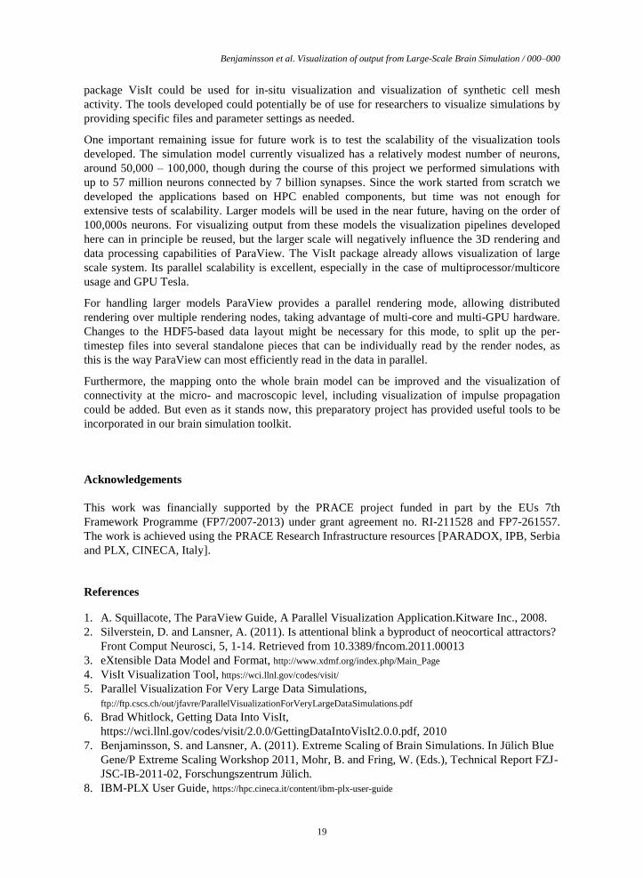
Another screenshot from the movie-like visualization for another time slice with a different

colourmap is shown in Fig. 13. The signals can be optionally visualized using a contour plot (Fig.

14).

Figure 13. Visualization using another colourmap (one

time slice from the movie-like presentation).

Figure 14. Visualization using a contour plot.

4. Conclusions

Considering the limited time available for this work quite good results were achieved, which will

form the basis for further work in the future. We were able to develop a workflow for visualization

of network activity of a brain region at both the single neuron and neuronal population levels,

together with realtime visualization of simulated network activity. The open source program


19

package VisIt could be used for in-situ visualization and visualization of synthetic cell mesh

activity. The tools developed could potentially be of use for researchers to visualize simulations by

providing specific files and parameter settings as needed.

One important remaining issue for future work is to test the scalability of the visualization tools

developed. The simulation model currently visualized has a relatively modest number of neurons,

around 50,000 – 100,000, though during the course of this project we performed simulations with

up to 57 million neurons connected by 7 billion synapses. Since the work started from scratch we

developed the applications based on HPC enabled components, but time was not enough for

extensive tests of scalability. Larger models will be used in the near future, having on the order of

100,000s neurons. For visualizing output from these models the visualization pipelines developed

here can in principle be reused, but the larger scale will negatively influence the 3D rendering and

data processing capabilities of ParaView. The VisIt package already allows visualization of large

scale system. Its parallel scalability is excellent, especially in the case of multiprocessor/multicore

usage and GPU Tesla.

For handling larger models ParaView provides a parallel rendering mode, allowing distributed

rendering over multiple rendering nodes, taking advantage of multi-core and multi-GPU hardware.

Changes to the HDF5-based data layout might be necessary for this mode, to split up the per-

timestep files into several standalone pieces that can be individually read by the render nodes, as

this is the way ParaView can most efficiently read in the data in parallel.

Furthermore, the mapping onto the whole brain model can be improved and the visualization of

connectivity at the micro- and macroscopic level, including visualization of impulse propagation

could be added. But even as it stands now, this preparatory project has provided useful tools to be

incorporated in our brain simulation toolkit.

Acknowledgements

This work was financially supported by the PRACE project funded in part by the EUs 7th

Framework Programme (FP7/2007-2013) under grant agreement no. RI-211528 and FP7-261557.

The work is achieved using the PRACE Research Infrastructure resources [PARADOX, IPB, Serbia

and PLX, CINECA, Italy].

References

1. A. Squillacote, The ParaView Guide, A Parallel Visualization Application.Kitware Inc., 2008.

2. Silverstein, D. and Lansner, A. (2011). Is attentional blink a byproduct of neocortical attractors?

Front Comput Neurosci, 5, 1-14. Retrieved from 10.3389/fncom.2011.00013

3. eXtensible Data Model and Format, http://www.xdmf.org/index.php/Main_Page

4. VisIt Visualization Tool, https://wci.llnl.gov/codes/visit/

5. Parallel Visualization For Very Large Data Simulations,

ftp://ftp.cscs.ch/out/jfavre/ParallelVisualizationForVeryLargeDataSimulations.pdf

6. Brad Whitlock, Getting Data Into VisIt,

https://wci.llnl.gov/codes/visit/2.0.0/GettingDataIntoVisIt2.0.0.pdf, 2010

7. Benjaminsson, S. and Lansner, A. (2011). Extreme Scaling of Brain Simulations. In Jülich Blue

Gene/P Extreme Scaling Workshop 2011, Mohr, B. and Fring, W. (Eds.), Technical Report FZJ-

JSC-IB-2011-02, Forschungszentrum Jülich.

8. IBM-PLX User Guide, https://hpc.cineca.it/content/ibm-plx-user-guide

http://www.xdmf.org/index.php/Main_Page

https://wci.llnl.gov/codes/visit/

ftp://ftp.cscs.ch/out/jfavre/ParallelVisualizationForVeryLargeDataSimulations.pdf

https://hpc.cineca.it/content/ibm-plx-user-guide


20

9. Lundqvist, M., Herman, P. and Lansner, A. (2011). Theta and gamma power increases and

alpha/beta power decreases with memory load in an attractor network model. J. Cogn. Neurosci.

10, 3008-3020.

10. Lundqvist, M., Compte, A. and Lansner, A. (2010). Bistable, Irregular Firing and Population

Oscillations in a Modular Attractor Memory Network. PLoS Comput. Biol. 6, e1000803.

visualization of output from large-scale brain simulations · visualization of output from...

Documents