VILNIAUS UNIVERSITETASFIZIKOS FAKULTETAS

TEORINĖS FIZIKOS KATEDRA

Jonas Narkeliūnas

A NUMERICAL APPROACH TO ESTIMATE THE BALLISTIC COEFFICIENT OF SPACEDEBRIS FROM TLE ORBITAL DATA

Mokslo tiriamasis darbas

(studijų programa – TEORINĖ FIZIKA IR ASTROFIZIKA)

Studentas Jonas Narkeliūnas

Darbo vadovas dr. Jan Stupl

Katedros vedėjas

Vilnius 2016

https://ntrs.nasa.gov/search.jsp?R=20160001336 2020-01-19T22:40:01+00:00Z

Contents

Introduction . . . . . . . . . . . . . . . . . . . . . . . . . . . . . . . . . . . . . . . . . . . . . . . . . . . . . . . . . . . . . . . . . . . . . . . . . . . . . . . . . . . . . . . . . . . . . . . . 31 Atmospheric Drag . . . . . . . . . . . . . . . . . . . . . . . . . . . . . . . . . . . . . . . . . . . . . . . . . . . . . . . . . . . . . . . . . . . . . . . . . . . . . . . . . . . . . 5

1.1 Drag Force and Drag Coefficient . . . . . . . . . . . . . . . . . . . . . . . . . . . . . . . . . . . . . . . . . . . . . . . . . . . . . . . . . . . 51.2 Atmospheric Density Model . . . . . . . . . . . . . . . . . . . . . . . . . . . . . . . . . . . . . . . . . . . . . . . . . . . . . . . . . . . . . . . . 7

2 Numerical Approach . . . . . . . . . . . . . . . . . . . . . . . . . . . . . . . . . . . . . . . . . . . . . . . . . . . . . . . . . . . . . . . . . . . . . . . . . . . . . . . . . . 102.1 Input Data . . . . . . . . . . . . . . . . . . . . . . . . . . . . . . . . . . . . . . . . . . . . . . . . . . . . . . . . . . . . . . . . . . . . . . . . . . . . . . . . . . . . 102.2 Ballistic Coefficient . . . . . . . . . . . . . . . . . . . . . . . . . . . . . . . . . . . . . . . . . . . . . . . . . . . . . . . . . . . . . . . . . . . . . . . . . . 122.3 Integration Using SGP4 . . . . . . . . . . . . . . . . . . . . . . . . . . . . . . . . . . . . . . . . . . . . . . . . . . . . . . . . . . . . . . . . . . . . . 132.4 Fast-Fourier Transformation . . . . . . . . . . . . . . . . . . . . . . . . . . . . . . . . . . . . . . . . . . . . . . . . . . . . . . . . . . . . . . . . 14

3 Results . . . . . . . . . . . . . . . . . . . . . . . . . . . . . . . . . . . . . . . . . . . . . . . . . . . . . . . . . . . . . . . . . . . . . . . . . . . . . . . . . . . . . . . . . . . . . . . . . . 18Conclusion . . . . . . . . . . . . . . . . . . . . . . . . . . . . . . . . . . . . . . . . . . . . . . . . . . . . . . . . . . . . . . . . . . . . . . . . . . . . . . . . . . . . . . . . . . . . . . . . . 24References . . . . . . . . . . . . . . . . . . . . . . . . . . . . . . . . . . . . . . . . . . . . . . . . . . . . . . . . . . . . . . . . . . . . . . . . . . . . . . . . . . . . . . . . . . . . . . . . . . 25

2

Introduction

Low Earth Orbit (LEO) is full of space debris, which consist of spent rocket stages, old satellites andfragments from explosions and collisions. As of 2009, more than 21 000 orbital debris larger than10 cm are known to exist [1], and while it is hard to track anything smaller than that, the estimatedpopulation of particles between 1 and 10 cm in diameter is approximately 500 000, whereas smallas 1 cm exceeds 100 million. These objects orbit Earth with huge kinetic energies – speeds usuallyexceed 7 km/s. The shape of their orbit varies from almost circular to highly elliptical and covers allLEO, a region in space between 160 and 2 000 km above sea level. Unfortunately, LEO is also theplace where most of our active satellites are situated1, as well as, International Space Station (ISS)and Hubble Space Telescope, whose orbits are around 400 and 550 km above sea level, respectively.This poses a real threat as debris can collide with satellites and deal substantial damage or evendestroy them.

Collisions between two or more debris create clouds of smaller debris, which are harder to trackand increase overall object density and collision probability. At some point, the debris density couldthen reach a critical value, which would start a chain reaction and the number of space debris wouldgrow exponentially. This phenomenon was first described by Kessler in 1978 and he concludedthat it would lead to creation of debris belt, which would vastly complicate satellite operations inLEO. [2].

The debris density is already relatively high, as seen from several necessary debris avoidancemaneuvers done by Shuttle, before it was discontinued, and ISS [1, 3, 4]. But not all satellites havea propulsion system to avoid collision, hence different methods need to be applied. One of the pro-posed collision avoidance concepts is called LightForce and it suggests using photon pressure toinduce small orbital corrections to deflect debris from colliding [5,6]. This method is very efficient– as seen from theoretical simulations, even few continuous mode 10 kW ground-based lasers, fo-cused by 1.5 m telescopes with adaptive optics, were enough to prevent significant amount of thedebris collisions. Simulations were done by propagating all space objects in LEO by 1 year into thefuture and checking whether the probability of collision was high. For those space objects differentground-based lasers were used to divert them, afterwards collision probabilities were reevaluated.However, the actual accuracy of the LightForce software, which has been developed at NASA AmesResearch Center, depends on the veracity of the input parameters, one of which is the object’s bal-listic coefficient. It is a measure of body’s ability to overcome air resistance, which has a significantimpact on the debris in LEO, and thus it is responsible for the shape of the trajectory of the de-bris. Having the exact values of the ballistic coefficient would make significantly better collisionpredictions, unfortunately, we do not know what are the values for most of the objects.

In this research, we were working with part of LightForce code, which estimates the ballis-

1Source: https://www.space-track.org.

3

tic coefficient from ephemerides2. Previously used method gave highly inaccurate values, whencompared to known objects, and it needed to be changed. The goal of this work was to try out adifferent method of estimating the ballistic coefficient and to check whether or not it gives noticeableimprovements in accuracy. Here we present our new approach and the ideas behind it.

2 Ephemeris (plural ephemerides) gives the position of astronomical objects as well as space debris in the sky at agiven time.

4

1 Atmospheric Drag

Everything above Karman line, 100 km above sea level, is assumed to be outer space, however,atmosphere extends far beyond that point. It extends for at least 10 000 km more [7], althoughafter 600 - 700 km it is not very significant (see Figure 1.1). Nevertheless, besides gravity, theatmospheric drag effect has the most impact on the object’s trajectory in LEO and it has to be takeninto account when modeling orbits of space objects in LEO. From here everything will eventuallyfall down to Earth, but the magnitude of the effect depends on many different parameters and wepresent them in this section.

1.1 Drag Force and Drag Coefficient

An object moving through medium always experiences drag – a resistance force acting in the op-posite direction of object’s movement. It is a result of three main effects: surface friction, flowinterference and form drag. At relatively high velocities and low densities, like in our case, thelateral effect overshadows the first two, so they can be neglected [9]. In this case, the drag force islargely proportional to characteristic area of the object and to the square of its velocity.

Figure 1.1 Variations of air density with height from 150 to 1000 km for high and low solar activityand diurnal variations (see chapter 1.2) based on COSPAR International Reference Atmosphere(CIRA 1972). Courtesy: King-Hele [8]

5

Using dimensional analysis from fluid dynamics, we can define drag as follows:

Fd =−1

2ρ

∣∣vrel2∣∣Cd A, (1.1)

where Fd is the drag force; ρ is a density of medium, in our case, the density of air; vrel is a relativevelocity of an object going through medium; and A is a characteristic area of that object. Cd is a dragcoefficient; it has no units and depends on the object’s surface roughness and shape, as seen fromFigure 1.2 – it also depends on the medium’s density and the molecular velocity [9]. Nevertheless,the dependence of different parameters for specific conditions are usually too small to take intoaccount, thus it is mostly used as a constant.

When modeling a space object, we usually do not know its shape, because this information is notsaved in ephemerides, as seen from chapter 2.1, hence we cannot know what is the exact value of thedrag coefficient. Even if we could capture an image of the object’s profile and measure the surfacearea, Cd and A values wouldn’t be right, as most of the objects are non-spherical and spinning withrespect to their direction of motion, hence one would need multiple pictures of different sides, aswell as, to know its angular velocity. A good way to deal with this is to approximate them as spheresand then use drag coefficient of a sphere. The value we use is Cd = 2.2, which was popularized bythe use of Jacchia models for estimating atmospheric density and other parameters of upper layers

Figure 1.2 Drag coefficient for different shape objects calculated at low velocities [10]

6

of Earth’s atmosphere [11, 12]. Note that this value is different from the one showed in Figure 1.2as a result of the following assumptions [9]:

• The mean free path of the air molecules is much greater than the size of the satellite.

• The satellite velocity v0 is much greater than the mean random velocity v of the air molecules.

• The mechanisms that deflect the impinging molecules range from elastic to inelastic impactand diffuse evaporation at an effective surface temperature T .

1.2 Atmospheric Density Model

As one can see, the drag force depends on the atmospheric density in different ways, but the densityis not constant. Even though we assume that its changes do little effect to the drag coefficient, forthe drag force we have to use accurate values, as objects closer to the ground will interact with it alot more and deorbit quicker than those who are further away; it is easy to see this from the ISS andVanguard 13 orbits. While the ISS is the biggest man-made satellite, it has one of the lowest orbitsof all artificial satellites and thus it loses 2 or more kilometers of altitude per month, as seen fromFigure 1.3. Without frequent orbital corrections it would deorbit within a year. Vanguard 1 is in ahigher orbit, with a perigee4 of 656 km and apogee5 of 3842 km (as of December 2015), and it isexpected to stay in orbit for 240 years 6.

Figure 1.3 Orbital height of the ISS throughout last year. Image source: www.heavens-above.com/ISSHeight.aspx

3Vanguard 1 is the oldest man made satellite still in orbit, launched in 1958; it was used to obtain geodetic mea-surements.

4A point where celestial body is closest to the Earth.5A point where celestial body is furthest from the Earth.6Retrieved from http://nssdc.gsfc.nasa.gov/nmc/spacecraftDisplay.do?id=1958-002B.

7

The Earth’s atmosphere is expanding and contracting in a complex manner all the time, not tomention it is not the same throughout different latitudes and longitudes. Many effects contribute tothat and a good atmospheric model should include at least most significant ones, if not all. Below,we list effects that are considered to be most important [13]:

• Latitudinal variations: The effect comes from satellite passing over the Earth’s equatorialbulge, effectively this changes the actual altitude and, therefore, the density.

• Diurnal variations: These variations come from the Earth’s rotation and the Sun’s irradia-tion. The day side of the Earth is warmer than the night side, hence the atmosphere expandsand bulges over ecliptic plane in the direction of the Sun. Because of the diurnal variations,it’s necessary to know latitude, local time, and time of the year.

• 27-day solar-rotation cycle: This effect arises from Sun’s rotation around its axis, whichcauses fluctuations in the amount of radiation that reaches the Earth.

• 11-year cycle of sunspots: Solar cycle strongly varies the amount of incoming radiationreaching the Earth. As a result, the Earth’s atmosphere heats up different amounts and itexpands different amounts throughout the cycle. At the solar maximum the temperature ofupper layers of the atmosphere is about two times higher than at solar minimum [14], meaningthat the atmosphere has expanded a lot more and debris will be affected more by the drag.In fact, nine times more debris fall to the surface of the Earth during solar maximum thanminimum [15]. Furthermore, depending on the altitude, this effect can even cause largerdisturbance through solar-radiation pressure than drag [13].

• Seasonal variations: These variations come from solar flux fluctuations due to Earth’s ro-tation around the Sun. The Earth’s rotational axis is tilted and its orbit is elliptical, thus theSun’s declination and the distance between the Earth and the Sun varies throughout the year.

• Rotating atmosphere: The atmosphere is rotating together with the Earth, however, thevelocity of lower layer is usually higher because of the friction with the Earth’s surface.

• Winds: Atmospheric winds and weather create local variations of the temperature and, there-fore, the density. Unfortunately, this is difficult to account for, as the weather itself is almostunpredictable because of its sensitivity to changes.

• Magnetic-storm variations: Effect comes from fluctuations in the Earth’s magnetic field,which affects the amount of charged particles reaching the Earth’s atmosphere from the Sun.

• Irregular short-periodic variations: Mostly solar flares: sudden increase in solar windintensity, which also disturbs the Earth’s magnetic field.

8

• Tides: Ocean tides and even atmospheric tides as a result of gravitational pull of the Mooncan cause small variations in the atmospheric density.

The first model of the Earth’s atmosphere above 120 km was created by Nicolet in 1961 [16]. Itwas an empirical model and used a set of boundary conditions of temperature and partial densitiesof gases altogether with diffusion theory to get values for higher altitudes. Later it was improvedupon several times by Jacchia with empirical data from the new satellites [11,17,18]. It was a goodmodel and even today it is still widely used for spacecraft dynamics. However, for more accuratecalculations like satellite and space debris orbital simulations, it is better to use a newer model,developed by Mike Picone, Alan Hedin, and Doug Drobof, which is called NRLMSISE-00 [19]. Itis an abbreviation of US Naval Research Laboratory and Mass Spectrometer and Incoherent ScatterRadar (00 stands for the year of release), the two primary data sources for development of earlierversions of the model.

NRLMSISE-00 is an empirical model of the Earth’s atmosphere from the ground through ex-osphere. Its outputs are atmospheric density, which we need, as well as temperature and otherparameters, while all the necessary input parameters are: year and day time of day; local apparentsolar time; geodetic altitude, latitude and longitude; daily and 81 day average of F10.7 solar flux7;daily geomagnetic index. This model includes most of the effects listed above [19], it is imple-mented in LightForce code and thus it is the perfect model for our simulations.

710.7 cm solar radio flux, F10.7, is a great indicator of solar activity, as it correlates with sunspots and UV radiation[14], as well as it is easy to measure it on the ground using radio antenna.

9

2 Numerical Approach

From the previous chapter we learned how the atmospheric drag affects the debris and why it variesin time, but the problem we face that it is very impractical to experimentally measure it withoutknowing the shape and the size of the debris. However, we can find ratios between mass, dragcoefficient and characteristic surface area of debris – the ballistic coefficient, and it can be donenumerically from the orbital tracking data. It is explained in this section.

2.1 Input Data

Satellite tracking began in 1957 with the launch of the first man-made satellite into space – Sputnik.The first methods for tracking used radio communication and weren’t very reliable as they couldn’tdetect or track objects in space that weren’t transmitting internationally agreed frequencies, as somedid. At that time, the main reason for satellite tracking was to defend against missile attacks, as aresult better methods were conceived. Telescopes with cameras were used instead, as well as radars,although they had their own limitations. Optical tracking systems depended on the weather andonly worked during night time, while radar was free from those problems, but it was costly [20].Nowadays the methods are the same, only the accuracy has increased a bit, albeit still relatively low,and objects as small as 1 cm could now be detected and tracked with ladars [21], which is great forestimating various parameters of the atmosphere, as well as predicting trajectories.

The most popular way for a celestial body’s detection and tracking is using a radar system. Thedetection is done by sending a powerful, yet short, impulse of radio signal into particular part ofspace and waiting for echoes. Computer analyzes the returned signal and from its strength, shapeand time in took to come back it calculates average ephemeris for that object [22]. Tracking, on theother hand, uses a priori knowledge where the object is going to be at specific time, so the radaris prepared by pointing to that part of the sky. After detection, it then tracks that object to get neworbital data, which is then saved as one data set. But there is only a finite number of radar sensorsites around the world, and they have a narrow view of the sky, and limited capabilities, meaningthat some space object aren’t in view all the time. Furthermore, they might not be in a good view ortracked for couple days, thus measurements are rare – from public database8 we see that it is aboutone per two days or less.

The format for storing ephemerides is the same as it was 50 years ago. Back then, a set of orbitalelements were written in two lines on a punch card9; from here came the name Two-Line Element(TLE) set, meaning this data encoding format. Given a reference frame and an epoch (a referencetime when ephemeris were taken), actually only six orbital elements are needed to unambiguously

8www.celestrak.com/NORAD/elements/9Punch card is a piece of stiff paper that contained either commands for controlling automated machinery or data

for data processing applications. Both commands and data were represented by the presence or absence of holes inpredefined positions.

10

define celestial body’s position and motion as a result of body having six degrees of freedom. Theseelements are as follows:

• Mean motion, n: Satellite’s average rate of motion over one orbit.

• Eccentricity, e: The shape of the orbit. 0 means circles; between 0 and 1 – ellipses; 1 –parabola; over 1 – hyperbola.

• Inclination, i : Tilt of the orbit plane relative to equatorial plane.

• Right ascension of the ascending node, Ω: The angle in the equatorial plane at which satel-lite crosses the equator from south to north, measured from Greenwich longitude.

• Mean anomaly, M : The angular distance from the perigee which a fictional body would haveif it moved in a circular orbit, with constant speed, in the same orbital period (true anomaly)as the actual body in its elliptical orbit.

• Argument of perigee, ω: The angle along the orbit between ascending node and perigeemeasured in the direction of motion.

These angles are showed in Figure 2.1. Here we showed only the most important elements of TLEset, albeit there are few more that help identify the object and its trajectory.

Figure 2.1 Orbital elements that define the position of celestial body. Note that instead of meananomaly a true anomaly is showed. Image source: www.wikipedia.com

11

These elements are our input data; from them we can calculate the ballistic coefficient, whichis used to predict the trajectory of the object. Formula for the ballistic coefficient is derived in thenext chapter.

2.2 Ballistic Coefficient

When debris or any other object moves through atmosphere it loses kinetic energy. This meansa decrease in total energy and it leads to orbital decay. Orbital decay can easily be seen fromdecreasing eccentricity and semi-major axis10, but we cannot know how much energy was lost,because we do not know object’s mass. Another way to calculate energy loss is from the work doneby drag force ((1.1) eq.)– by integrating drag force over the path that debris travels. As mentioned inthe previous chapter, for those calculations we need characteristic area and drag coefficient, however,we do not know them either. Fortunately, these two energies are almost the same and, by neglectingthe energy fluctuations induced by gravitational field perturbations, we can have an equality:

rˆr0

1

2ρCd A |vrel|

(vrel ·dr′

)' µm

r− µm

r0+ mv2

0

2− mv2

2. (2.1)

Here µ is the gravitational constant times the Earth’s mass; r is the distance from the center ofmass and v is the object’s velocity relative to the Earth’s surface. The left-hand side was alreadyintroduced in previous section. Note that when we are calculating relative velocity to Earth’s at-mosphere, vrel, we are assuming atmosphere rotating with Earth with angular velocity ω⊕withoutwinds as that would be impossible to predict. It is expressed with the following equation:

vrel = v−ω⊕× r. (2.2)

In (2.1) eq., everything but the mass, characteristic area and drag coefficient, can be calculatedor is known from the tracking data. However, the unknowns actually give us the ballistic coefficient

B = m

Cd A, (2.3)

whose estimation is the main goal of this work. Thus from (2.1) formula we can derive an equationfor estimating the ballistic coefficient, and it is as follows:

B = m

Cd A'´ t

t0ρ |vrel| (vrel ·v)d t ′

2µ(

1a(t ) − 1

a(t0)

) ≈∑N

i=1ρ |vrel| (vrel ·v)∆t

2µ(

1a(t ) − 1

a(t0)

) (2.4)

In the numerator we changed integration over the distance to integration over the time, hence the10Semi-major axis is a popular unit in the field of astrodynamics. It is defined as half the distance of the longest

principal axis of an elliptical orbit. For circular orbits it coincides with radius.

12

object’s velocity relative to the atmosphere is now multiplied by velocity. For numerical approachwe also changed integration with summation, thus we introduced ∆t , which is an arbitrary sizeof time step, and N = t−t0

∆t . While in the denominator we expressed total energy per mass unit as

a function of semi-major axis using this equation: a =(

2r − v2

µ

)−1. This was done as it is more

convenient to calculate ballistic coefficient from TLE set data. Hence now we have a formula forthe ballistic coefficient estimation and we can solve it numerically.

2.3 Integration Using SGP4

Orbital elements define space object’s orbit and motion, but for our calculations they are not easyto use. It is useful to transform them to a different state vector – a position vector and a velocityvector, which we can use in the (2.4) equation. The best way to get the state vector is to use SGP4propagator – a simplified general perturbation model, which was purposely designed to work withthe TLE set data [23]. As the name implies, this model uses simplified perturbations to modelorbit of the space object. Simplifications were done by assuming static atmosphere and includingonly the biggest perturbations of gravitational field as well as guessing the value of the ballisticcoefficient. Also, SGP4 propagator can estimate the object’s state vector for any arbitrary point intime, although its predictions are limited by its accuracy, as even small state vector errors start togrow exponentially over time. This is mostly due to it using its own estimate of ballistic coefficientcalculated from one TLE set, which, as mentioned previously, is not perfectly accurate.

In the 2.1 chapter, we mentioned that TLE sets are rare – about one TLE per two days, thenon average we have around two hundred TLE data sets per one year. It is clearly not enough for anaccurate summation in (2.4) eq. as we are describing changes of the velocity and the atmosphericdensity that are happening in minute scale and not day scale, as showed in Figure 2.2. Nevertheless,in the old method it is done with even less. Even though the approach is different, the idea behindit is very similar to the new method. It calculates semi-major axis decay per orbit from averagevalues of only few TLE sets and using the same averaged values it integrates to find the drag effectfor one orbit. From here, similarly like in (2.4) eq., it is possible to estimate the ballistic coefficient.However, using averaged values, especially from small pool of TLE sets, it gives biggest errors ofthis method.

On the other hand, in the new method we are trying to capture all of those details, thus we needmore data points and for this reason we are using SGP4 propagator to generate it. Even though theaccuracy of the model degrades exponentially by every day since the epoch [24], we are only usingit for short propagations. From Levit et al article [25], it is clear that propagating about 2 days isstill accurate as errors are less than 1 km for most debris, after that it is best to take have new TLEset from the next epoch. Fortunately, SGP4 can propagate forwards and backwards in time, thus wecan have a total difference of 4 days between any two TLE sets without sacrificing accuracy of ourcalculations.

13

For a better accuracy of estimating the ballistic coefficient we would need a very small time step∆t , in the orders of seconds, however, these calculations would take extremely long time and that isinconvenient. By experimenting with different values we noticed that it is best to use time step of 1minute. It means that we have about 100 data points per orbit (LEO satellite’s period is around 100minutes) which is enough to capture the atmospheric density changes throughout different parts ofthe orbit.

2.4 Fast-Fourier Transformation

The numerical data generated by SGP4 propagator includes a lot of physical phenomena that makethe energy and thus the semi-major axis oscillate throughout the orbit and time. This effect canbe easily seen in the Figure 2.2 where we plotted debris’s semi-major axis over time using SGP4generated data. Interestingly enough, from the original TLE set data (generated state vector atTLE epoch) it would appear that debris’s orbital height is increasing. With more data, even if it isgenerated by SGP4 propagator, we can capture intrinsic behavior of the semi-major axis and see thatoriginal TLE set data is only a snap-shots of that, thus first assumption would have been most likelyfalse. By our guess, the illusion of growing orbit can be created by orbital precession – rotation ofthe orbit itself, which is not included in the original TLE set data. By plotting yet another object’ssemi-major axis values over time in top Figure 2.3 we can actually see oscillations of semi-majoraxis over time scale that is not explained by any other phenomena, thus supporting this idea. Asshown in bottom Figure 2.3, if the celestial body is observed from the same spot on the Earth, likeusing the same radar or telescope site, it will detect the body at different sections of its the orbit.This can be supported by the fact that from the semi-major axis plot it is visible that TLE sets arealmost equally spaced, meaning that measurements are periodical and it is most likely to be true ifthe same observatory is taking ephemerides of that debris.

Looking into the lower Figure 2.2, we can also see that oscillations are so big that they actuallyhide any changes that happen to the semi-major axis due to the drag effect. Up until now theseoscillations were necessary for the accurate orbit determination but now they are overshadowingthe evaluation of the semi-major axis decay. Using this data would lead to the negative ballisticcoefficient and our estimation would be most likely wrong. Although sometimes negative valuesare meaningful, as some satellites have propulsion systems and can do orbital maneuvers, like theISS, but most of them are debris or passive satellites and should naturally decay. Actually, we expectto find more than 95 % of celestial bodies to have a positive decay values [1] as only few percentare working satellites and out of them only few have propulsion, but first we need additional step –filter the data.

From all the phenomena that are affecting semi-major axis we can only include those whocause drag fluctuations – the rest we must remove. This is a necessary step because otherwise(2.4) eq. becomes invalid. By writing that equation, we neglected gravitational perturbations, so

14

from SGP4 dataSe

mi-m

ajor

axi

s (k

m)

Time (Julian days)

Figure 2.2 Semi-major axis over time. Black squares are semi-major axis at TLE epoch, green lineare generated by propagating from epoch. All data generated using SGP4 propagator. Satellite’scatalog number: NORAD 299

that semi-major axis decay could be written as equal to energy lost due to drag. Thus we have thesame thing here, we must remove gravitational perturbations, which are caused by a non-sphericalgravity (the Earth has a non-uniform mass distribution) and a three-body gravity (Moon, Earth andSun) [13, 23]. Lateral effect will cause long-periodic and short-periodic variations of the semi-major axis, while the non-spherical gravity will only cause the short-periodic variations. By short-periodic, we mean oscillations on the same scale as celestial body’s orbital period; while the long-periodic variations are above tens of days. Knowing this, we can remove these effects by applyingFourier transformation to SGP4 propagator generated data [26]. However, to accurately do it, wefirst need to remove non-periodic energy decay, which is caused by all of the phenomena. This canbe easily done by applying simple linear regression to find line fit of the data: slope k and interceptb:

k = x y − x y

x2 − x2;

b = y −kx, (2.5)

and subtracting the fitted line from the data. In this case, we are left with pure oscillations with nodecay and algorithm for fast Fourier transformation (FFT) can be used, although here we will not

15

5550 5600 5650 57007339,7

7339,8

7339,9

7340,0

7340,1

Sem

i-maj

or a

xis

(km

)

Time (Julian days)

from TLE set data

Figure 2.3 Top: The semi-major axis over time of the object NORAD 7646. Bottom: Satellite’sorbital precession around The Earth. For an observer standing still on one point of the Earth itappears that satellite’s orbit declines

16

5540 5550 5560 5570 5580 5590 5600 5610

7384,874

7384,941

7385,008

7392,567

7392,580

7392,593Se

mi-m

ajor

axi

s (k

m)

Time (Julian days)

TLE set After FFT

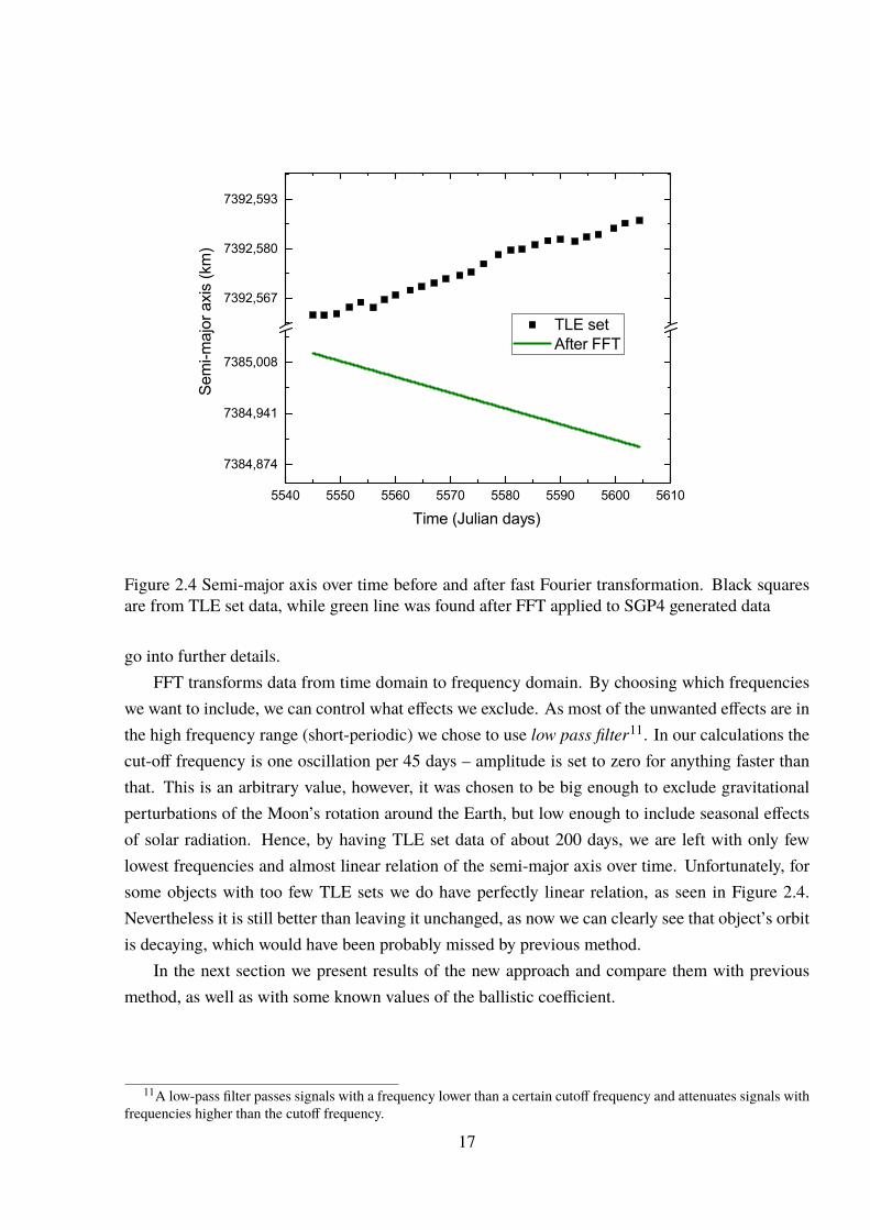
Figure 2.4 Semi-major axis over time before and after fast Fourier transformation. Black squaresare from TLE set data, while green line was found after FFT applied to SGP4 generated data

go into further details.FFT transforms data from time domain to frequency domain. By choosing which frequencies

we want to include, we can control what effects we exclude. As most of the unwanted effects are inthe high frequency range (short-periodic) we chose to use low pass filter11. In our calculations thecut-off frequency is one oscillation per 45 days – amplitude is set to zero for anything faster thanthat. This is an arbitrary value, however, it was chosen to be big enough to exclude gravitationalperturbations of the Moon’s rotation around the Earth, but low enough to include seasonal effectsof solar radiation. Hence, by having TLE set data of about 200 days, we are left with only fewlowest frequencies and almost linear relation of the semi-major axis over time. Unfortunately, forsome objects with too few TLE sets we do have perfectly linear relation, as seen in Figure 2.4.Nevertheless it is still better than leaving it unchanged, as now we can clearly see that object’s orbitis decaying, which would have been probably missed by previous method.

In the next section we present results of the new approach and compare them with previousmethod, as well as with some known values of the ballistic coefficient.

11A low-pass filter passes signals with a frequency lower than a certain cutoff frequency and attenuates signals withfrequencies higher than the cutoff frequency.

17

3 Results

For our calculations, we only used TLE set data12 from the year 2015. Part of the data, from January1st till August 15th, was used for the ballistic coefficient calculation, while the rest, from August16th to September 15th, was used to analyze the accuracy of the estimated values. In general, wewould want to extend the first period as we want to have as many TLE sets as possible for a moreaccurate estimation, however, this work was done by focusing on implementing the new approachand checking whether or not it works better than previously used method, and for this reason weused the same data as was used in previous calculations.

Furthermore, at this stage software is incapable of allocating memory for more than 200 TLEsets, albeit from Figure 3.1 we see that most objects have fewer number of TLE sets. Actually, mostobjects have as few as 14 TLE sets, while average value is 75. Note that these results came afterdoing initial data filtration, which removed outliers (data points that are more than 2σ away fromthe mean) and TLE sets that are too much separated in time to have a good estimation by SGP4propagator, as explained in chapter 2.3. These steps reduced the total number of available TLE setssubstantially, leading to distribution we see in Figure 3.1.

Whenever we estimate the ballistic coefficient for the whole catalog of tracked objects (>13 000)it takes two whole days, plus an additional day if we want a least squares fitting13 on top of that.The least squares fitting algorithm was already implemented in the code and it usually improves the

20 40 60 80 100 120 140 160 180 2000

50

100

150

200

250

300

Num

ber o

f obj

ects

Number of TLE sets

Mean

Maximum

Figure 3.1 Number of objects with different number of TLE sets. Data collected from the periodJanuary 1st to August 15th of 2015

12All data was downloaded from www.space-track.org.13Least squares fit is a statistical method that minimizes the sum of squares of the errors made in the results of every

single equation.

18

accuracy of the ballistic coefficient. It uses a high precision propagator to propagate the trajectory,while TLE snapshots are used as virtual observations for the fit. Nevertheless, the least squaresfit uses our estimated values of the ballistic coefficient as its initial guesses, even though it is verysensitive to local minimum, meaning that after this step values are still quite similar. As this stepspecifically is unrelated to this work, we only did it to compare the new results with the old onesand they were calculated by the previous approach plus the least squares fitting. Unfortunately, dataanalysis is difficult, as we don’t know anything about the true values of the ballistic coefficient ofthe debris and most satellites. We can only compare our results with some (not all) that we knowand whose shape is simple, like sphere, cylinder or cube, as well their mass and size is known. Inthis case, we can manually calculate the ballistic coefficient using the same formula as in (2.3) eq.,where Cd = 2.2 is the drag coefficient of the sphere. This data is showed in Table 3.1.

By looking at the Table 3.1, we can see that in many cases the new approach is significantlybetter than the old one. Albeit it is still underestimating the ballistic coefficient by about one orderof magnitude. Most likely this could happen, if the atmospheric drag is weaker than it should havebeen, which could have been caused by partly underrated atmospheric density. By plotting accu-racy of the ballistic coefficient (a ratio between the estimated value and real value) against object’sinclination, as it is done in Figure 3.2, we can actually see a correlation between the two. Onecan see that for all space objects, whose orbits are equatorial (orbital plane is parallel to equator),the accuracy of the ballistic coefficient is significantly worse than for the objects, whose orbits areinclined or even perpendicular to equatorial plane. This relationship between accuracy and inclina-tion can be explained by underestimating bulging of the Earth’s atmosphere. Albeit NRLMSISE-00includes effects like that, SGP4 doesn’t – it uses simple model of static atmosphere, as mentioned inchapter 2.3. In the previous approach SGP4 propagator isn’t used in the same manner as in the newmethod, thus there is no reason for it to exhibit similar behavior throughout different inclinationsand should show no correlation – that is what we see in Figure 3.2.

19

20 40 60 80 100

1E-3

0,01

0,1

1

Estimated New BC/ True BC Estimated Old BC/ True BC

Rel

ativ

e de

viat

ion

Inclination (degree)

Figure 3.2 Accuracy of the ballistic coefficient of the old (red) and the new (navy blue) methodsplotted against inclination. Accuracy is measured as a ratio between estimated value and “true”value

20

Table 3.1 Comparison of the true ballistic coefficient versus estimated value for satellites with simple shapesName NORAD ID Mass (kg) Dimensions (m)/Shape Inclination Apogee/Perigee (km) Eccentricity Btr ue B new

est. B ol dest .

STARLLETE 7646 47.3 ;0.24/sphere 49.8 1107/805 0.15679 475 64.7 0.60AJISAI 16908 685 ;2.15/sphere 50.0 1503/1485 0.00602 85.8 3.41 0.90

STELLA 22824 48.0 ;0.24/sphere 98.6 805/797 0.00499 482 165 0.76LARES 38077 387 ;0.36/sphere 69.5 1456/1445 0.00379 1728 151 16.4DANDE 39267 38.0 ;0.46/sphere 81.0 1390/328 0.61816 104 74.6 59.9

KIKU 1 (ETS 1) 8197 85.0 ;0.9/spherical 47.0 1109/981 0.06124 60.7 14.9 1.79NADEZHDA 2 20508 870 ;2×3.5/cylindrical 83.0 1023/960 0.03177 126 18.4 -

SCD 1 22490 115 ;1×1/cylindrical 25.0 782/720 0.01664 66.6 0.45 6.85FORTE 24920 41.0 ;0.8×2/cylindrical 70.0 825/798 0.01664 37.1 7.05 0.41

ORSTED 25635 50.0 0.34×0.45×8.72/rectangular 96.5 833/632 0.13720 148 24.4 1.91PCSAT 26931 10.0 0.253/cube 67.0 795/787 0.00506 37.3 7.60 0.80

FEDSAT 27598 50 0.583/cube 98.4 811/797 0.00871 69.3 29.9 0.86LATINSAT B 27606 12 0.253/cube 64.6 727/598 0.09736 89.6 11.3 4.48

SAUDISAT 1C 27607 10 0.233/cube 64.6 709/596 0.08659 88.2 9.29 3.84AAU CUBESAT 27846 1 0.13/cube 98.7 833/818 0.00909 46.7 11.7 1.29

SEEDS 32791 1 0.13/cube 96.7 617/597 0.01647 46.7 25.9 33.1VESSELSAT 1 37840 29.0 0.33/cube 20.0 874/854 0.01157 150 0.081 34.4

SRMSAT 37841 10.4 0.283/cube 20.0 875/856 0.01098 61.9 0.036 3.66TUGSAT-1 39091 7.00 0.23/cube 98.6 790/776 0.00894 40.8 46.4 0.69CASSIOPE 39265 500 ;1.8×1.25/cylindrical 81.0 1358/329 0.60996 89.3 56.4 38.6

DRAGONSAT 39383 1.00 0.13/cube 40.5 402/402 0 46.7 2.30 46.8COOPER 39395 1.00 0.13/cube 40.5 336/319 0.02595 46.7 2.16 36.3AIST 1 39492 39.0 0.47×0.56×0.48/rectangular 82.4 628/599 0.02363 72.8 51.8 30.2

21

Another way of checking the accuracy of our method is by launching body propagator, imple-mented in Lightforce software. By putting calculated values of the ballistic coefficient as a newinput, we can see how much object’s position deviates from the TLE set data that was not used forthe estimation of the ballistic coefficient. Furthermore, we can do the same with values from theold approach, hence we can compare the accuracy of both methods against each other and againstexperimental measurements. Here, we chose to propagate only 4 geodetic satellites14, as they arespherical in shape and in theory should show best results. Results are plotted in Figure 3.3.

It is easy to see that in all examples the new method performs better than the old one. Positionalerrors of the new method are significantly smaller, sometimes by two orders of magnitude smaller,like in graphs of AJISAI and STELLA. Here we can see that even after two months the positionalerrors are relatively small and not growing exponentially. By looking at the graph of AJISAI satel-lite, we can even see that the expected position of the satellite was on the other side of the Earththan it really was after 25 days of propagation with the old approach. Oscillations visible in thesame graph are actually caused by our imaginary satellite going around the Earth and catching upwith real one. Only in the graph of satellite DANDE we see similarly bad performance, albeit theestimated values of the ballistic coefficient for DANDE are closest to the real value out of all foursatellites. This could be caused by highly elliptical orbit, as out of all four it has the highest eccen-tricity. STARLETTE has the second biggest value of eccentricity and the positional errors in timeexhibit similar behavior. Thus highly elliptical orbits might pose another problem for the accuracyof calculations.

Lastly, when we looked throughout the list of all tracked space objects and their estimatedvalues of the ballistic coefficient, we calculated the percentage of the objects with negative values.We found that there is only 4.57 of the objects with such values. In chapter 2.4, we emphasizedthat less than 5% of tracked objects are active satellites, although few of them do have propulsionsystem, we can see that the new method gives absolutely wrong values for only couple of percentsof tracked objects. On the other hand, the old approach gives almost one fourth of the time (26.04%)negative values, which is at least 5 times worse, when compared to the new approach.

14The geodetic group of satellites are inactive targets for satellite laser ranging that are used for positioning, gravi-tational field modeling and atmospheric modeling.

22

0 2 4 6 8 10 12 14

0

100

200

300

400

500

600

-5 0 5 10 15 20 25 30 35 40

0

1000

2000

3000

4000

5000

0 10 20 30 40 50 60 7010

100

1000

10000

0 10 20 30 40 50 6010

100

1000

10000

New B = 64.8 Old B = 0.60

New B = 74.6 Old B = 59.9

STARLETTE DANDE

AJISAI STELLA

New B = 3.41 Old B = 0.01

Posi

tiona

l erro

r (km

)

New B = 164 Old B = 0.76

Time (Days)

Figure 3.3 Positional errors calculated using the new approach (navy blue) and the old approach (red). x-axis are days of propagation. Notedifferent time scales

23

Conclusion

• The new approach implemented in the Lightforce code gives significantly better results whencompared to the old version of the code. The new estimated values are mostly within oneorder of magnitude away from the real values, usually being underestimated, while the olderones were mostly two or more orders of magnitude away.

• We showed that the accuracy of the new approach is inclination dependent while this is notvisible in the previous method. We suspect that errors arise from SGP4 model underestimat-ing the Earth’s atmospheric density at equatorial plane, which is consistent with the resultsfrom the geodetic satellites.

• When propagating object’s trajectory with new values, we see a lot smaller positional errorsfrom previously used method. Positional errors are two orders of magnitude smaller thanthey were before, thus Lightforce simulations can now be used to predict real collision threatswithin moderate accuracy.

24

References

[1] The Threat of Orbital Debris and Protecting NASA Space Assets from Satellite Collisions,Technical report, National Aeronautics and Space Administration (2009).

[2] D. J. Kessler, B. G. Cour-Palais, Collision frequency of artificial satellites: The creation of adebris belt, Journal of Geophysical Research: Space Physics (1978–2012) 83(A6), 2637–2646(1978).

[3] K. T. Alfriend, M. R. Akella, J. Frisbee, J. L. Foster, D.-J. Lee, M. Wilkins, Probability ofcollision error analysis, Space Debris 1(1), 21–35 (1999).

[4] J. L. Foster Jr, The analytic basis for debris avoidance operations for the international spacestation, in Space Debris (2001), volume 473, 441–445.

[5] J. Stupl, J. Mason, W. Marshall, C. Levit, C. Smith, S. Olivier, A. Pertica, W. De Vries,LightForce: Orbital collision avoidance using ground-based laser induced photon pressure,in C. Phipps (ed.), American Institute of Physics Conference Series (2012), volume 1464 ofAmerican Institute of Physics Conference Series, 481–491.

[6] J. Stupl, N. Faber, C. Foster, F. Y. Yang, B. Nelson, J. Aziz, A. Nuttall, C. Henze, C. Levit,Lightforce photon-pressure collision avoidance: Updated efficiency analysis utilizing a highlyparallel simulation approach, in Advanced Maui Optical and Space Surveillance TechnologiesConference (2014), volume 1, 9.

[7] S. Bauer, H. Lammer, Planetary Aeronomy. Atmosphere Environments in planetary Systems,1610-1677 (Springer-Verlag Berlin Heidelberg, 2004), 1 edition.

[8] D. G. King-Hele, Satellite orbits in an atmosphere: theory and application (Springer Science& Business Media, 1987).

[9] R. Stirton, The upper atmosphere and satellite drag, Smithsonian contributions to astrophysics5(2) (1960).

[10] L. Clancy, Aerodynamics, Pitman Aeronautical Engineering Series (Wiley, 1975).

[11] L. G. Jacchia, Static diffusion models of the upper atmosphere with empirical temperatureprofiles, Smithsonian Contributions to Astrophysics 8, 215 (1965).

[12] B. R. Bowman, K. Moe, Drag coefficient variability at 175–500 km from the orbit decayanalyses of spheres, Advances in the Astronautical Sciences 123.1, 117–136. (2005).

[13] D. A. Vallado, Fundamentals of Astrodynamics and Applications (Microcosm Press, 2013),fourth edition.

25

[14] K. F. Tapping, The 10.7 cm solar radio flux (f10.7), Space Weather 11(7), 394–406 (2013).

[15] N. Johnson, Space debris issues, Audio File, @0:05:50-0:07:40. The Space Show (2011).

[16] M. Nicolet, Structure of the thermosphere, Planetary and Space Science 5(1), 1–32 (1961).

[17] L. G. Jacchia, Revised static models of the thermosphere and exosphere with empirical tem-perature profiles, Smithsonian Astrophysical Observatory Special Report (332) (1971).

[18] L. G. Jacchia, Thermospheric temperature, density, and composition: new models, SAO spe-cial report 375 (1977).

[19] J. M. Picone, A. E. Hedin, D. P. Drob, A. C. Aikin, Nrlmsise-00 empirical model of theatmosphere: Statistical comparisons and scientific issues, Journal of Geophysical Research:Space Physics 107(A12), SIA 15–1–SIA 15–16, 1468 (2002).

[20] D. G. King-Hele, Review of tracking methods, Philosophical Transactions of the Royal Societyof London. Series A, Mathematical and Physical Sciences 262(1124), 5–13 (1967).

[21] B. Greene, Y. Gao, C. Moore, Laser tracking of space debris, in 13th International Workshopon Laser Ranging Instrumentation, Washington DC (2002).

[22] D. Mehrholz, L. Leushacke, W. Flury, R. Jehn, H. Klinkrad, M. Landgraf, Detecting, trackingand imaging space debris, ESA Bulletin (0376-4265) (109), 128–134 (2002).

[23] F. R. Hoots, R. L. Roehrich, Spacetrack report no. 3, Colorado Springs CO: Air ForceAerospace Defence Command 1–3 (1980).

[24] D. A. Vallado, P. Crawford, R. Hujsak, T. Kelso, Revisiting spacetrack report no. 3, AIAA6753, 2006 (2006).

[25] C. Levit, W. Marshall, Improved orbit predictions using two-line elements, Advances in SpaceResearch 47(7), 1107 – 1115 (2011).

[26] J. W. Cooley, J. W. Tukey, An algorithm for the machine calculation of complex fourier series,Mathematics of computation 19(90), 297–301 (1965).

26

Jonas Narkeliūnas

SKAITMENINIŲ METODŲ TAIKYMAS KOSMINIŲ ŠIUKŠLIŲ BALISTINIOKOEFICIENTO APSKAIČIAVIMUI, PASITELKIANT TLE ORBITINIUS DUOMENIS

Santrauka

Kosminės šiukšlės yra auganti bėda, su kuria tenka susidurti bet kuriam bandančiam sėkmingaivystyti tyrimus žemutinėje Žemės orbitoje. Kosminės šiukšlės yra sudarytos iš panaudotų raketiniųvariklių, nebeveikiančių palydovų ir skeveldrų, pažertų po sprogimų ir susidūrimų tarp tų pačiųnuolaužų, ir jos skrieja aplink Žemę su milžiniškomis kinetinėmis energijomis. Net mažiausiašiukšlė/skeveldra lekianti 7 km/s greičiu gali perskrosti saulės elementus, o vos 1 cm dydžio galinet pažeisti korpusą raketos gabenančios žmones ar krovinius. Didžiausią grėsmę šiuo metu joskelią Tarptautinei Kosminiai Stočiai (TKS), kurioje nuolat yra grupė žmonių – būtent dėl šiukšliųTKS tenka atlikinėti įvairius manevrus, kad išvengtų susidūrimo rizikos. Tačiau nevisi dirbtiniaipalydovai turi raketinius variklius, tad jie neturi galimybės išvengti susidūrimo. Jam įvykus, paly-dovas gali būti sunaikintas ir tapti nauju kosminių šiukšlių debesiu, kuris atsitiktinai gali pataikytiį dar kitus palydovus ar tas pačias kosmines šiukšles. Pasiekus tam tikrą kritinį tankį šis proce-sas pradės dažnėti eksponentiškai ir kosminių šiukšlių skaičius sparčiai išaugs. Tuomet žemutinėŽemės orbita bus tankiai užpildyta kosminėmis šiukšlėmis ir nebus galima vykdyti jokios veiklos,tad akivaizdu, kad kosminės šiukšlės kelią didelį pavojų tiek dabartiniams palydovams, tiek ateityjeplanuojamoms kosminėms misijoms.

Jau šiuo metu kosminių šiukšlių koncentraciją yra didelė ir, jei nieko nebus imtasi, o paly-dovų bus keliamą į orbitą vis daugiau, tai šis scenarijus greitai išsipildys. Dėl šios priežasties yravystomos įvairios koncepcijos kosminių šiukšlių susidūrimų mažinimui ir jų pašalinimui. Vienatokia koncepcija vadinasi LightForce – tai yra simuliacijų paketas, skirtas sumodeliuoti ir įvertintiar galima išvengti kosminių šiukšlių susidūrimų naudojant antžeminius lazerius [5]. LightForceprognozuoja, kuriuos kosminės šiukšlės susidurs, ir prieš tam įvykstant, truputį pakeičia jų greičiuspasitelkiant lazerio šviesos pluoštus taip, kad jos saugiai prasilenktų. Teoriškai jau yra įrodyta, kadšitas metodas yra veiksmingas, tačiau prieš pritaikant programą praktiniams bandymams reikiapagerinti jos prognozių tikslumą. Pastarosios labai priklauso nuo balistinio koeficiento vertės, kurinusako, kaip smarkiai ar silpnai objekto trajektoriją paveiks oro pasipriešinimas. Tačiau balistiniskoeficientas kosminėms šiukšlėms yra nežinomas, kadangi jis priklauso nuo masės ir charakteringoploto, taip pat ir nuo pasipriešinimo koeficiento, priklausančio nuo objekto formos, o šių duomenųtiesiogiai išmatuoti mes negalime. Tokiu atveju balistinis koeficientas yra ieškomas netiesiogiaiiš orbtinių duomenų, pasitelkiant skaitmeninius metodus. Vis dėlto ankstesnėje programos versi-joje naudoti skaitmeniniai metodai davė pakankamai netikslias balistinio koeficiento vertes, o taireiškia, kad objektai galėjo būti toli nuo prognozuotų pozicijų, tad netiksliai buvo prognozuojami

ir susidūrimai. Šio darbo tikslas buvo pagerinti balistinio koeficiento apskaičiavimo metodą.Šiame darbe išvedėme naują formulę balistinio koeficiento apskaičiavimui, kurią galima skait-

meniškai išspręsti iš turimų orbitinių duomenų. Siekiant geresnio tikslumo taip pat pritaikėme įvair-ius duomenų tvarkymo ir papildomų duomenų generavimo metodus. Gauti rezultatai parodė, kadkiekybiškai naujasis metodas duoda net pora eilių tikslesnes vertes lyginant su ankstesniu metoduir tikromis balistinio koeficiento vertėmis (tikros vertės gali būti apskaičiuojamos žinomos formos,dydžio ir masės palydovams). Taip pat naudojant naujas vertes gaunamos žymiai geresnės prog-nozės palydovo trajektorijai, tad ir susidūrimai gali būti geriau įvertinti negu anksčiau. Taigi aki-vaizdžiai sugebėjome pagerinti programos veikimą – simuliacijų tikslumą.

28