Nanand 

  Final Version

   Authors

Nicole MEmpa –

Prof. DrEmpa –

nomad land

l report

: August 20

s:

Müller and PMaterials S

r. Jing WangMaterials S

ateriadfills 

t 

012 

PD Dr. BernScience and

g, Dr. AndreScience and

als in

d NowackTechnology,

ea Ulrich andTechnology,

n was

y, Technolog

d Dr. Jelenay, Laboratory

te inc

gy and Socie

a Buha y for Analyt

ciner

ety lab

ical Chemis

ration

stry

n 

2

This study was funded by the Swiss Federal Office for the Environment (BAFU). How to cite this report: Mueller, N.C.; Nowack, B.; Wang, J. Ulrich, A.; Buha, J. (2012) Nanomaterials in waste incineration and landfills. Internal Empa-report. Available at: http://www.empa.ch/plugin/template/empa/*/124595 Contact: PD Dr. Bernd Nowack Environmental Risk Assessment and Management Group Empa-Swiss Federal Laboratories for Materials Science and Technology Lerchenfeldstrasse 5 CH - 9014 St. Gallen Switzerland nowack@empa.ch

3

Summary In the past, waste incineration processes had been identified as an important source of ultrafine air pollutants resulting in elaborated treatment systems for exhaust air. Today, these systems are able to remove around 99.99% of all ultrafine particles as measured in a Swiss waste incineration plant. However, the fate of ultrafine particles caught in the filters has received little attention until now. Studies investigating the size distribution of fly ash from waste incineration plants so far focused on micro-sized particles. Based on the recent developments in nanotechnology and the resulting increase in the application of engineered nano-objects (ENO), it can be expected that not only combustion generated nanoparticles are found in fly ash but also ENO. This study aimed at identifying the total nano-fraction of fly ash (weight and particle number) from waste, wood and sludge incineration in Switzerland by particle size measurements and to compare it to the modeled amount of ENO as well as to the modeled amount of nanoparticles derived from conventional pigments. In addition, first measurements were made to analyze the size distribution of fly ash before and after acid washing. The results allow a first estimation of the importance of ENO for waste streams in Switzerland.

In the analytical part, samples from different waste, wood and sludge incineration plants were pre-fractionated at 2 µm. The mass fractions were determined by weighing and a Laser Diffraction Particle Size Analyzer was used to determine the particle size distribution (mass and particle number) before and after pre-fractionation. A more detailed analysis of the size distribution for the below-2-µm fraction was performed using a powder disperser for aerosolization and measurements for size distribution by scanning mobility particle sizer (SMPS) for the size fraction between 15 and 660 nm and by an aerodynamic particle sizer (APS) for the size fraction from 0.5 to 20 µm. The data from both methods were fitted to receive an overall size distribution curve. In the modeling part, a model was generated which allowed a quantitative prediction of the expected ENO flows to waste incineration and landfills. The input flows were taken from Gottschalk et al. (2009). The model- and substance-specific coefficients were extrapolated based on the limited literature available.

Typical SMPS data for fly ashes showed a minor peak at around 100 nm and the main size distribution peak at around 270 nm. APS measurements indentified the largest particle fraction around 1 µm. These curves were merged to a single size distribution from 15 nm – 20 µm. Based this new curve the mass fraction and number percentage of the fly ash particles <100 nm were calculated. In average only about 0.00079wt% of the fly ash samples were found to be nano-sized and below 10% of the particle number.

The modeling showed that - despite several differences between the models for nano-TiO2, nano-ZnO and nano-Ag (e.g. partial dissolution of nano-ZnO in acid washing) - the major ENO-flow goes from the waste incineration plant to the landfill as bottom ash. All other flows within the system boundary were about one magnitude smaller than the bottom ash flow. A different ENO distribution was found for CNT. CNT as carbon-based material are expected to burn to a large extent (94%) so that only insignificant amounts remain in the system.

In Switzerland about 80’000 t of fly ash are produced in waste and sludge incineration per year. Another 40’000 t of fly ash is formed during wood incineration. According to the measurements in this study, a fraction of about 0.00058wt% of the sludge and waste

4

incineration fly ash is <100 nm, which results in 464 kg per year. The nano-sized fraction from wood incineration is slightly higher at 0.0039wt% (1.56 t/a). In contrast, the modeling calculates an amount of 22 t/a TiO2-ENO, 0.8 t/a ZnO-ENO, 160 kg/a Ag-ENO and 4.9 kg/a of CNT in fly ash, which is significantly higher than the measured total nano-fraction in the fly ash. This discrepancy can be explained by the measurement method and the morphology of nano-objects. Ultrafine particles such as ENO tend to agglomerate very quickly and form stable agglomerates of several hundred nanometers. Our method of aerosolization is representative for the processes handling of fly ash and thus quantifies the possible release of nano-sized material from fly ash. This proclivity has been confirmed by Scanning Electron Microscopy-analyses of ENO after incineration. Since the measurements in this study were based on size fractionation without prior breaking of agglomerates, agglomerates were measured as large particles. Hence, the number and mass of primary nanoparticles in our measurements is probably significantly underestimated whereas the modeling calculates the mass of primary ENO, which might in fact be existent as agglomerates. Quantitative microscopy analyses of the fly ash samples taken are needed to complement the results of the measurements.

5

Content

1  Motivation and goal of the study .................................................................................................................................. 7 

2  Introduction ............................................................................................................................................................................ 8 

3  Literature survey ................................................................................................................................................................. 13 

3.1  Characterization (size distribution and chemical composition) of combustion residues from

domestic waste, wood and sewage sludge ................................................................................................................. 13 

3.1.1  General behavior of different compounds during combustion ...................................................... 14 

3.1.2  Incineration of household residues ............................................................................................................ 15 

3.1.3  Wood incineration ............................................................................................................................................ 20 

3.1.4  Sludge incineration ........................................................................................................................................... 21 

3.1.5  Engineered nano-objects (ENO) in waste incineration ....................................................................... 21 

3.2  Characterisation of pigments (TiO2, SiO2, ZnO, carbon black) regarding their share of

nanosized particles ................................................................................................................................................................ 23 

3.3  Nanomaterials in landfills .................................................................................................................................... 24 

3.3.1  Characterization of landfill leachate regarding its content of metallic particles <0.45 µm . 24 

3.3.2  Behavior of ENO in landfill ............................................................................................................................. 25 

4  Particle size distribution of fly ashes and pigments ............................................................................................ 26 

4.1  Sample description ................................................................................................................................................ 26 

4.1.1  Fly Ashes ............................................................................................................................................................... 26 

4.1.2  Pigments ............................................................................................................................................................... 27 

4.2  Particle size measurements ................................................................................................................................ 27 

4.2.1  Determination of the particle size distribution in fly ashes .............................................................. 28 

4.2.2  Determination of the particle size distribution in commercial pigments ................................... 31 

4.3  Results ......................................................................................................................................................................... 32 

4.3.1  Size distribution of fly ashes from waste, sludge and wood incineration plants ..................... 32 

4.3.2  Size characterization of different TiO2 and ZnO pigments................................................................ 38 

5  Modeling ............................................................................................................................................................................... 40 

5.1  Methods ..................................................................................................................................................................... 40 

5.1.1  Model description ............................................................................................................................................. 40 

5.1.2  Model parameters (input parameters, coefficients) ............................................................................ 41 

6

5.2  Results ......................................................................................................................................................................... 45 

5.2.1  Modeling of nano-TiO2 flows to the landfills ......................................................................................... 45 

5.2.2  Modeling of nano-ZnO flows to the landfills ......................................................................................... 46 

5.2.3  Modeling of nano-Ag flows to the landfills ............................................................................................ 48 

5.2.4  Modeling of CNT flows to the landfills ..................................................................................................... 50 

5.2.5  Calculation of bulk-derived nano-objects ............................................................................................... 52 

6  Discussion ............................................................................................................................................................................. 54 

6.1  Measurements ......................................................................................................................................................... 54 

6.2  Modeling .................................................................................................................................................................... 55 

6.2.1  Limitations of the model ................................................................................................................................ 55 

6.2.2  Interpretation of the modeling data .......................................................................................................... 57 

6.3  Synthesis and interpretation of measurement and modeling data ................................................... 57 

7  Outlook .................................................................................................................................................................................. 61 

8  Conclusion ............................................................................................................................................................................ 62 

9  Glossary ................................................................................................................................................................................. 63 

10  References ...................................................................................................................................................................... 64 

7

1 Motivation and goal of the study

This project aims to provide a first estimation of the amount of engineered nano-objects (ENO) ending up in landfills and their contribution to fly ash originating from waste and sludge incineration. For this purpose it is prerequisite to differentiate ENO from nano-sized fractions of conventional bulk materials and from ultra-fine particles generated by combustion during the incineration processes.

In the first part, a literature review was performed to obtain size-dependent and elemental information about fly and bottom ashes from municipal waste, wood or sludge incineration as well as to collect the information known about the behavior of ENO in waste incineration.

In the second part, size distributions (particle mass and number concentration) of typical fly ashes originating from six selected incineration plants in Switzerland were investigated and the mass-percentage of the nano-fraction was determined. In addition first measurements were performed to analyze the size distribution of fly ash before and after acid washing. Similar measurements were carried out to characterize the size distribution of titanium oxide and zinc oxide pigments commonly used in paint. These latter results fed into the modeling carried out in the third part.

In the third part, a model to estimate the flows of ENO and bulk-derived materials into the different types of landfills was elaborated. The results obtained from the literature study and the measurements of the fly ash were compared to the modeled input of ENO and bulk-derived nanomaterials into waste and sludge incineration to estimate their importance for waste streams in Switzerland.

8

2 Introduction

Nanotechnology and the resulting engineered nanomaterials have gained raising interest not only in research and development but also in the public and at regulatory authorities [1]. The interest in nanotechnology increases constantly due to various superior properties of nanoparticles compared to conventional materials. Nanoparticles exhibit rich physical and chemical phenomena, and their fascinating and unusual properties have opened up myriad applications in industry, medicine and other applications with the promise of many more.

On the other hand, widespread nanoparticle applications are suspected to cause mostly unknown consequences to human health and the environment [2]. Concerns have been raised on the potential toxicity of such tiny particles as the damaging effects of exposure to unintentionally produced ultrafine particles (e.g. by combustion processes) have been proven [3, 4]. Nanomaterials according to the International Organisation for Standardisation (ISO) are materials with any internal or external dimension/structure from 1-100 nm [5] (Fig. 1). This term is very broad including a wealth of conventional materials. However, relevant from a (eco)toxicological perspective is the sub-category named “nano-objects” which defines particles, plates or fibers with at least one external dimension between 1-100 nm (Fig. 1). The term “engineered” is added to restrict the nano-objects to intentionally produced materials. Numerous products containing engineered nano-objects (ENO) are already on the market ranging from antibacterial textiles [6, 7] with nanoscale silver particles (nano-Ag) to high performance batteries with carbon nanotubes (CNT), self-cleaning paints [8, 9] and coatings with photocatalytically active nanoscale titanium dioxide particles (nano-TiO2) or sunscreens making use of nanoscale zinc oxide (nano-ZnO). Even if the number of products is still relatively low (currently estimated to be less than about 1 % [10, 11]), the trend is increasing. Release studies are still rare [7, 8, 12, 13] and analyses especially in complex matrices or the environment are challenging [2, 14]. Only little knowledge is available focusing on end-of-life treatment of nanomaterials, i.e. waste treatment like incineration [15, 16], deposition on landfills or recycling possibilities.

During the last years the number of publications related to toxicity and ecotoxicity of ENO has increased enormously, but studies on the (eco)toxicity of ENO are not always conclusive and long-term studies are still missing [17]. However, it is confirmed that the toxicity is not only determined by the nano-size of the particle but more importantly by the chemical composition of the substance. In addition several physico-chemical characteristics, such as coatings and shape can influence the toxicity of the material [18, 19].

 

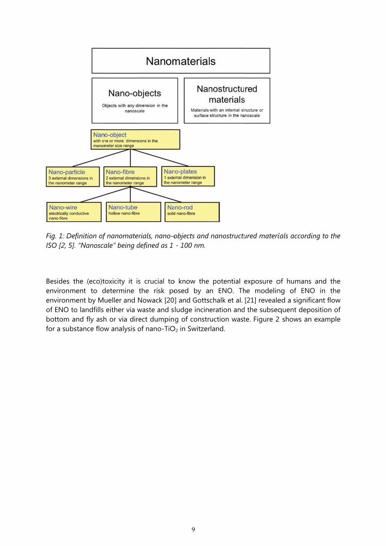
Fig. 1: DISO [2, 5

Besides environenvironof ENO bottom for a su

Definition of5]. “Nanosca

the (eco)tment to dment by Muto landfills and fly ash

bstance flow

f nanomaterale” being d

oxicity it isdetermine tueller and Neither via w

h or via direw analysis o

rials, nano-odefined as 1

s crucial tothe risk poNowack [20]waste and sect dumpinof nano-TiO

9

objects and - 100 nm.

o know the osed by a] and Gottsludge incing of constr

O2 in Switzer

nanostructu

potential n ENO. Thchalk et al. eration and

ruction wastrland.

 

ured materi

exposure ohe modelin[21] reveale

d the subseqte. Figure 2

ials accordin

of humans ng of ENOed a significquent depo

2 shows an

ng to the

and the O in the cant flow osition of example

10

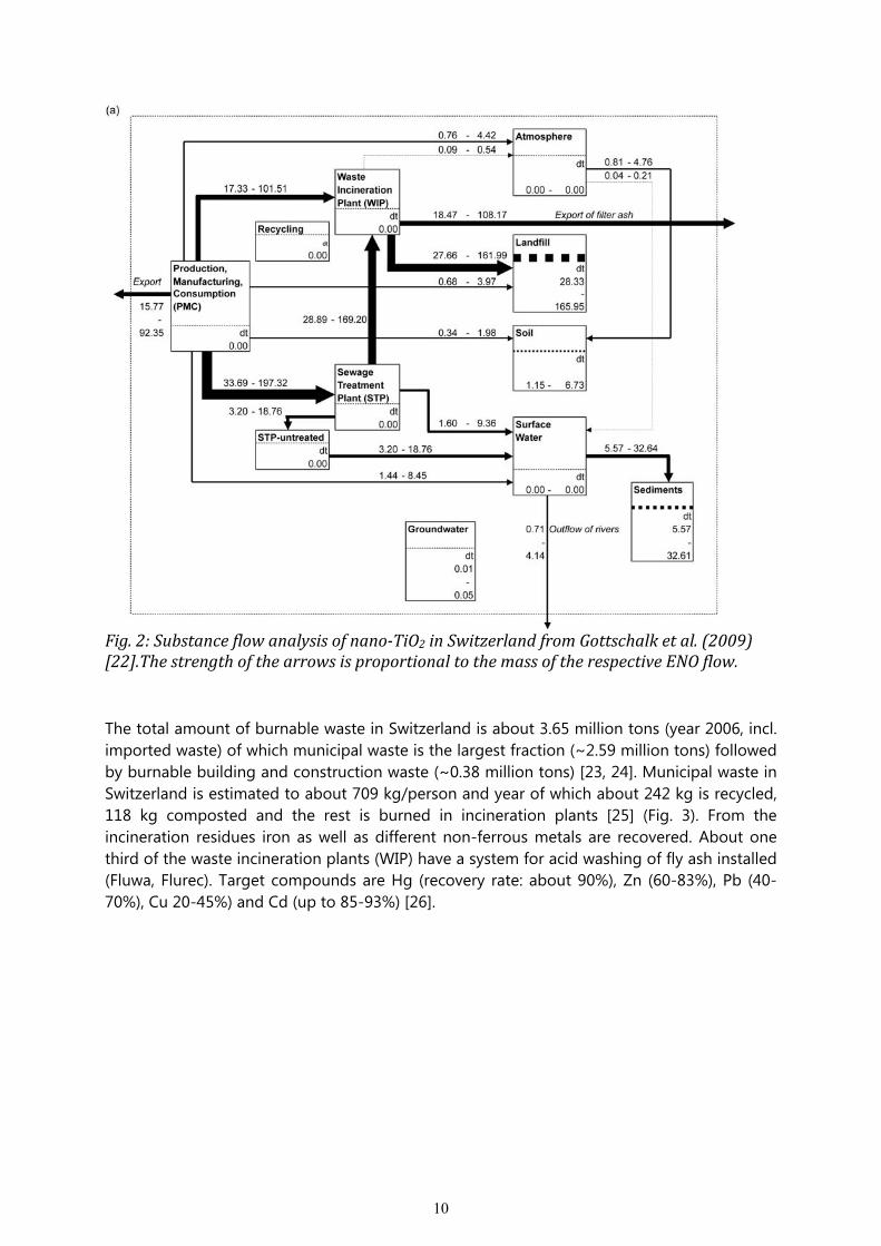
Fig.2:Substanceflowanalysisofnano‐TiO2inSwitzerlandfromGottschalketal.(2009)[22].ThestrengthofthearrowsisproportionaltothemassoftherespectiveENOflow.

The total amount of burnable waste in Switzerland is about 3.65 million tons (year 2006, incl. imported waste) of which municipal waste is the largest fraction (~2.59 million tons) followed by burnable building and construction waste (~0.38 million tons) [23, 24]. Municipal waste in Switzerland is estimated to about 709 kg/person and year of which about 242 kg is recycled, 118 kg composted and the rest is burned in incineration plants [25] (Fig. 3). From the incineration residues iron as well as different non-ferrous metals are recovered. About one third of the waste incineration plants (WIP) have a system for acid washing of fly ash installed (Fluwa, Flurec). Target compounds are Hg (recovery rate: about 90%), Zn (60-83%), Pb (40-70%), Cu 20-45%) and Cd (up to 85-93%) [26].

11

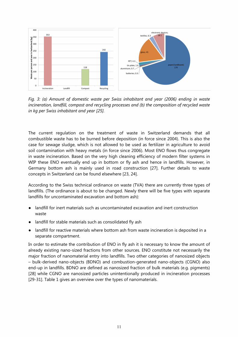
Fig. 3: (a) Amount of domestic waste per Swiss inhabitant and year (2006) ending in waste incineration, landfill, compost and recycling processes and (b) the composition of recycled waste in kg per Swiss inhabitant and year [25].

The current regulation on the treatment of waste in Switzerland demands that all combustible waste has to be burned before deposition (in force since 2004). This is also the case for sewage sludge, which is not allowed to be used as fertilizer in agriculture to avoid soil contamination with heavy metals (in force since 2006). Most ENO flows thus congregate in waste incineration. Based on the very high cleaning efficiency of modern filter systems in WIP these ENO eventually end up in bottom or fly ash and hence in landfills. However, in Germany bottom ash is mainly used in road construction [27]. Further details to waste concepts in Switzerland can be found elsewhere [23, 24].

According to the Swiss technical ordinance on waste (TVA) there are currently three types of landfills. (The ordinance is about to be changed. Newly there will be five types with separate landfills for uncontaminated excavation and bottom ash):

● landfill for inert materials such as uncontaminated excavation and inert construction waste

● landfill for stable materials such as consolidated fly ash

● landfill for reactive materials where bottom ash from waste incineration is deposited in a separate compartment.

In order to estimate the contribution of ENO in fly ash it is necessary to know the amount of already existing nano-sized fractions from other sources. ENO constitute not necessarily the major fraction of nanomaterial entry into landfills. Two other categories of nanosized objects – bulk-derived nano-objects (BDNO) and combustion-generated nano-objects (CGNO) also end-up in landfills. BDNO are defined as nanosized fraction of bulk materials (e.g. pigments) [28] while CGNO are nanosized particles unintentionally produced in incineration processes [29-31]. Table 1 gives an overview over the types of nanomaterials.

paper/cardboard; 170

batteries; 0.3

aluminium; 0.7

tin plate; 1.6

PET; 4.3

glass; 41

textiles; 6.3

electronic devices; 18.1353

118

242

0

50

100

150

200

250

300

350

400

Incineration Landfill Compost Recycling

Waste per person and year in Switzerlan

d [kg] 

12

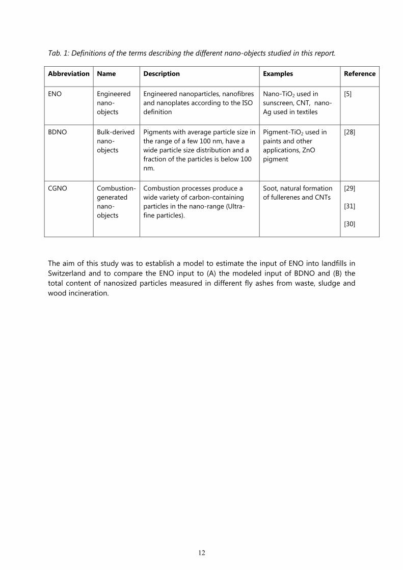
Tab. 1: Definitions of the terms describing the different nano-objects studied in this report.

Abbreviation Name Description Examples Reference

ENO Engineered nano-objects

Engineered nanoparticles, nanofibres and nanoplates according to the ISO definition

Nano-TiO2 used in sunscreen, CNT, nano-Ag used in textiles

[5]

BDNO Bulk-derived nano-objects

Pigments with average particle size in the range of a few 100 nm, have a wide particle size distribution and a fraction of the particles is below 100 nm.

Pigment-TiO2 used in paints and other applications, ZnO pigment

[28]

CGNO Combustion-generated nano-objects

Combustion processes produce a wide variety of carbon-containing particles in the nano-range (Ultra-fine particles).

Soot, natural formation of fullerenes and CNTs

[29]

[31]

[30]

The aim of this study was to establish a model to estimate the input of ENO into landfills in Switzerland and to compare the ENO input to (A) the modeled input of BDNO and (B) the total content of nanosized particles measured in different fly ashes from waste, sludge and wood incineration.

13

3 Literature survey

3.1 Characterization (size distribution and chemical composition) of combustion residues from domestic waste, wood and sewage sludge

In the past, waste incineration processes had been identified as an important source of ultrafine air pollutants [32] resulting in elaborated treatment systems for exhaust air. Today, these filter systems are able to remove around 99.99% of all ultrafine particles [33]. In most cases the exhaust air released from incineration plants into the environment easily meets the standards for air quality. In Switzerland, the introduction of the Ordinance on Air Pollution Control (OAPC) / Luftreinhalteverordnung (LRV) in 1986 led to significant investments in the infrastructure of the WIP regarding the reduction of emissions. For many pollutants, the WIP are not a relevant source anymore. Especially the emission of ultrafine particles was reduced to a total of 30 t per year which corresponds to only a few per mills of the total emissions of ultrafine particles in Switzerland [23]. Based on this development in the past 15-20 years, it is not surprising that, thus far, research on waste incineration has focused on the emission of ultrafine particles and other pollutants into the air. A wealth of studies reports on particle size and composition of the material released at the stack. However, almost no studies are available investigating size-distribution and particle number concentration of ultrafine particles caught in the filters. The fate of such residues has received little attention until now.

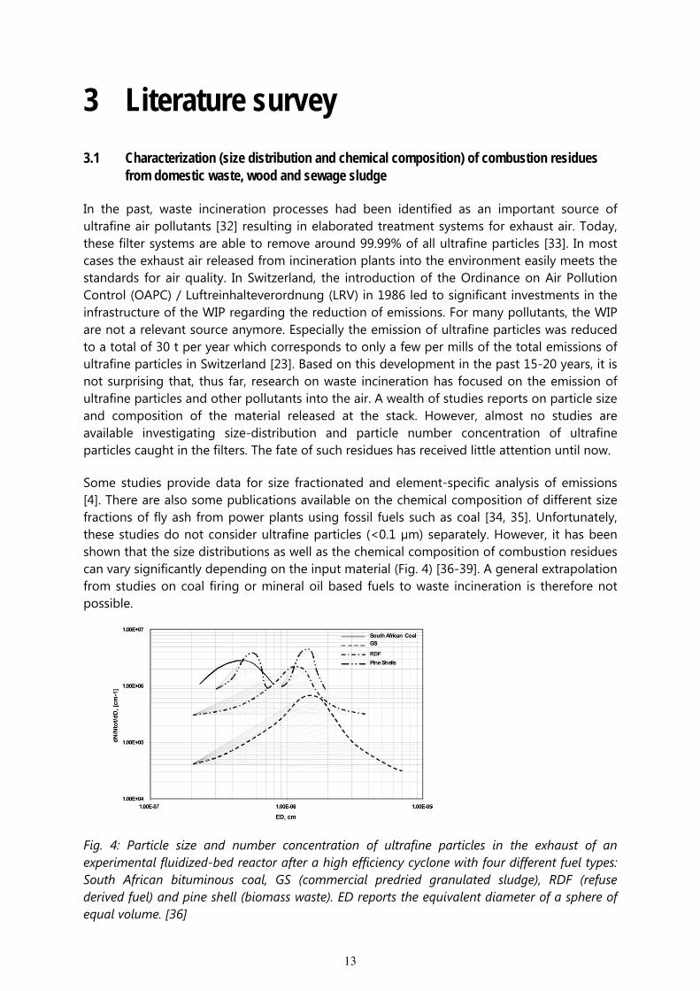
Some studies provide data for size fractionated and element-specific analysis of emissions [4]. There are also some publications available on the chemical composition of different size fractions of fly ash from power plants using fossil fuels such as coal [34, 35]. Unfortunately, these studies do not consider ultrafine particles (<0.1 µm) separately. However, it has been shown that the size distributions as well as the chemical composition of combustion residues can vary significantly depending on the input material (Fig. 4) [36-39]. A general extrapolation from studies on coal firing or mineral oil based fuels to waste incineration is therefore not possible.

Fig. 4: Particle size and number concentration of ultrafine particles in the exhaust of an experimental fluidized-bed reactor after a high efficiency cyclone with four different fuel types: South African bituminous coal, GS (commercial predried granulated sludge), RDF (refuse derived fuel) and pine shell (biomass waste). ED reports the equivalent diameter of a sphere of equal volume. [36]

14

However, in view of the lack of data, nonetheless a few studies from heating plants were included as a baseline for the estimation of the size distribution and chemical composition of nano-sized fly ash fraction in the following chapter.

3.1.1 General behavior of different compounds during combustion

General studies on the distribution of different elements in fly ash and bottom ash reveal the dependency on the elements’ physico-chemical properties [39]. Metals may be volatilized during combustion based on the incineration temperature and the volatility of the respective compound [37]. A reducing atmosphere and a high Cl content in the fuel may enhance (trace) metal vaporization during combustion [37]. Meij et al. distinguish three classes of elements according to their distribution in fly ash in comparison to bottom ash from a Dutch coal firing plant [34]. Elements in the first class (class I) do not vaporize during incineration and hence their concentrations are similar in all ash-types. Examples for such class I elements are Al, Ca, Ce, Fe, K, Mg, Si and Ti. Class II elements such as Mn, Na, Ni and Zn are enriched in fly ash. These elements volatilize (based on their boiling point) during high temperature combustion. As the temperature drops in the exhaust, they pass their dew points and hence nucleation or condensation starts on the surface of fly ash particles. Since small particles have a larger specific surface area, they are found to have the greatest concentration of Class II elements. Class III elements are mainly gaseous compounds that are usually emitted in the gas phase (e.g. B, Br, Cl, F and S).

A slightly different categorization was suggested by Querol et al. [35]. The authors distinguish elements with volatile behavior that (partially) condense in flue gases and thus enrich in fly ash (e.g. As, B, Bi, Pb, S, Cd), elements that are concentrated in the slag (e.g. C, Fe and elements with iron oxide affinity such as Cu, or Mn) and elements that show no fractionation between fly ash and slag (e.g. Al, Ca, Na, Mg, Li, Cr, Co, Ni, Zn). According to Querol et al. elements with calcium oxide-sulfate affinities enrich in fly ash. Sorum et al. [40] found Cd, Hg and Pb fully volatilized at a temperature of 950° C. The state of aggregation of elements like As, Cu, Ni and Zn strongly depends on the temperature, the fuel/air ratio and the availability of Cl and S [40]. Evans et al. summarized: “Volatile mercury and cadmium compounds with high vapour pressures and low boiling points are most likely to be found in the flue gas. Metals with a medium vapour pressure and boiling points, such as lead and zinc, are retained better in the slag and are less concentrated in the fly ash. Other metals with low vapour pressure and high boiling points, such as iron and copper, are almost completely trapped in the bottom ash.” In terms of the “nano”-relevant elements (e.g. Ti, Ag, Ce, Zn, Fe, C), the element Fe was mostly found to be enriched in bottom ash. Silver (Ag) was not classified. Ti and Ce were mentioned to show almost no segregation. For Zn only a slight enrichment in fly ash was observed in the study by Querol et al. and thus Zn was categorized as non-fractionating element, while Meij et al. classified Zn as element enriching in fly ash. According to Sorum et al. [40], the distribution of Zn to fly ash and bottom ash depends on the redox-conditions in the furnace.

Several authors have further analyzed the distribution of various elements within different size fractions of the fly ash. Querol et al. [35] found most of the elements studied (e.g. Cd, Cr, Cu, Na, Ni, Pb, S, Sn and Zn) concentrated 2-20 times in the finest fraction (0.3 µm – 10 µm) while carbonaceous materials appeared in higher concentrations in larger particle fractions. Fe, Ca, Al, K, Li, Mg, Mn, P and Ti showed no dependency on particle size [35]. Generally the

15

fine fraction (<40 µm) of the fly ash analyzed by Arditsoglou et al. accounted for a relatively small percentage (5-10 %) of the total fly ash mass [41]. This study showed that for each element analyzed around 5-15 % of the total mass was found in the fraction below 40 µm. This corresponded fairly well to the total mass fraction of the fine particles (5-10 %). Hence, the authors found no significant enrichment of any element in the finest fraction of the fly ash for Al, Ca, Cr, Cu, Fe, Ge, K, Mg, Ni, P, Pb, S, Se, Si, Ti and Zn. However, for PAH it was shown that the PAH-concentration in the finest fly ash fraction is for many PAH-compounds lower than in larger fractions [41]. Itskos et al. [42] found the following composition of fly ash particles smaller than 25 µm: 27.3% SiO2, 37.1% CaO, 12.4% SO3, 0.7% K2O, 0.5% Na2O, 0.5% TiO2, 2.4% MgO, 14.5% Al2O3 and 4.6% Fe2O3. In comparison larger fly ash particles had a significantly higher share of SiO2, Al2O3 and Na2O, but a lower share of CaO and SO3 [42]. Bhattacharjee et al. estimated the particle size distribution from fly ash of a thermal power plant in India by SEM images. They found particles from 0.16–5.50 mm with a main composition from O, Al, Si, C, Fe, Mg, Na, K and Ti [43].

Another important factor affecting the chemical composition and size distribution of fly ash is the filter type [44]. In Swiss wood, sludge and waste incineration plants either bag house filters or electrostatic precipitators (ESP) are installed. In bag house filters, additives (e.g. Ca(OH)2 [37], NaHCO3, active carbon) may be added for the precipitation of volatile acids or gaseous components like dioxins/furans as well as heavy metals. The amount of additives added may be significantly higher than the total amount of fly ash particles itself (personal communication, Häuselmann).

 

3.1.2 Incineration of household residues

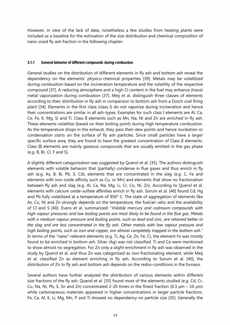
A study on the filter efficiency in waste incineration plants in Switzerland has shown that ESP are able to retain around 99.5% of all ultrafine particles (Fig. 5) [33]. From the remaining particles another 98.5% are removed by the subsequent treatment processes, wherewith 99.99% of the ultrafine particles end up in the filter ash.

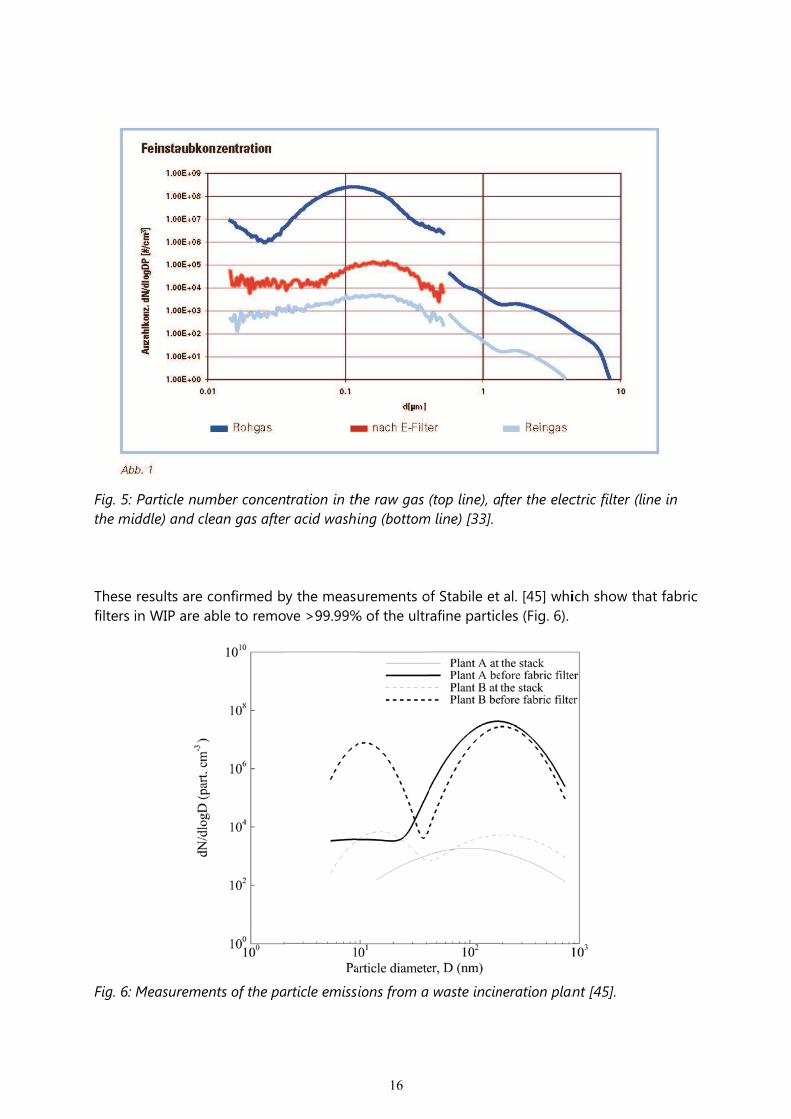
Fig. 5: Pthe midd

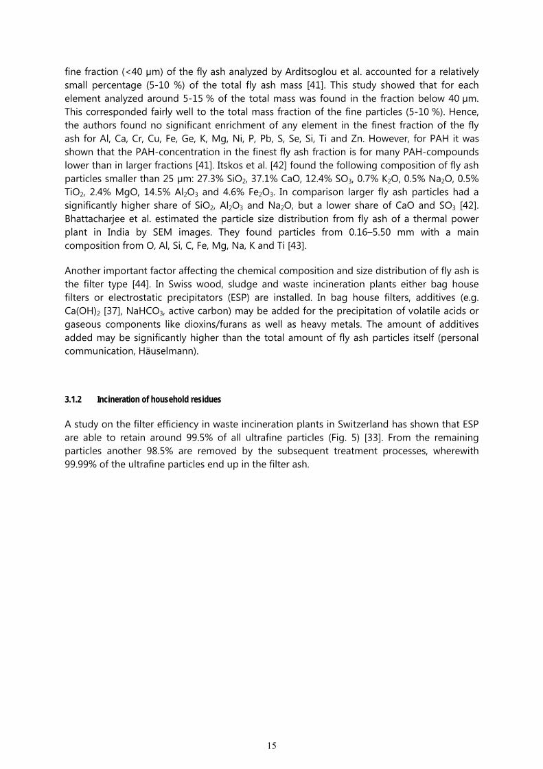
These refilters in

Fig. 6: M

Particle numdle) and cle

esults are cn WIP are ab

Measuremen

mber concenean gas after

onfirmed byble to remo

nts of the pa

tration in thr acid washi

y the measuve >99.99%

article emiss

16

he raw gas ing (bottom

urements o% of the ultr

ions from a

(top line), am line) [33].

of Stabile et rafine partic

waste incin

fter the elec

al. [45] whiles (Fig. 6).

neration plan

ctric filter (li

ich show th

nt [45].

ine in

hat fabric

17

Chang and Wey [46] studied the composition of fly ash and bottom ash in a waste incinerator in Taiwan. In an average Taiwanese WIP 10-15% of the waste input results in bottom ash and 2-3% are collected as fly ash. Of the fly ash 0 – 30 wt% were below 53 µm depending on the waste incinerator studied (Fig. 7a). Of the bottom ash 5 – 30 % were below 180 µm (Fig. 7b).

a) 

b)

Fig. 7: Particle size distribution given as percentage of weight (a) in fly ash and (b) in bottom ash from three municipal solid waste incinerators [46].

 

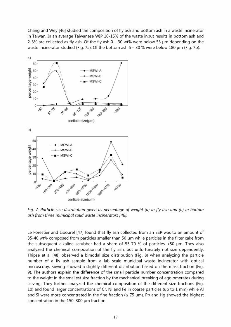
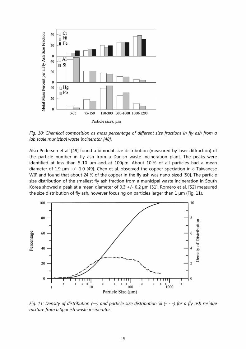
Le Forestier and Libourel [47] found that fly ash collected from an ESP was to an amount of 35-40 wt% composed from particles smaller than 50 µm while particles in the filter cake from the subsequent alkaline scrubber had a share of 55-70 % of particles <50 µm. They also analyzed the chemical composition of the fly ash, but unfortunately not size dependently. Thipse et al [48] observed a bimodal size distribution (Fig. 8) when analyzing the particle number of a fly ash sample from a lab scale municipal waste incinerator with optical microscopy. Sieving showed a slightly different distribution based on the mass fraction (Fig. 9). The authors explain the difference of the small particle number concentration compared to the weight in the smallest size fraction by the mechanical breaking of agglomerates during sieving. They further analyzed the chemical composition of the different size fractions (Fig. 10) and found larger concentrations of Cr, Ni and Fe in coarse particles (up to 1 mm) while Al and Si were more concentrated in the fine fraction (≤ 75 µm). Pb and Hg showed the highest concentration in the 150–300 µm fraction.

  

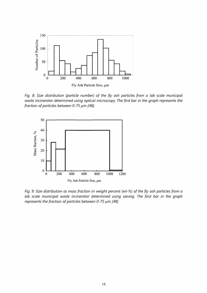
Fig. 8: Swaste infraction

 

 

Fig. 9: Slab scalrepresen

 

Size distribuncinerator d

of particles

Size distributle municipants the fract

ution (particdetermined us between 0-

tion as masal waste inction of partic

cle number)using optica-75 µm [48]

s fraction incinerator decles between

18

) of the flyal microscop].

n weight peretermined n 0-75 µm [

ash particlpy. The first

rcent (wt-%using sievin[48].

les from a bar in the g

%) of the fly ang. The firs

lab scale mgraph repres

ash particlest bar in th

municipal sents the

es from a he graph

19

Fig. 10: Chemical composition as mass percentage of different size fractions in fly ash from a lab scale municipal waste incinerator [48].

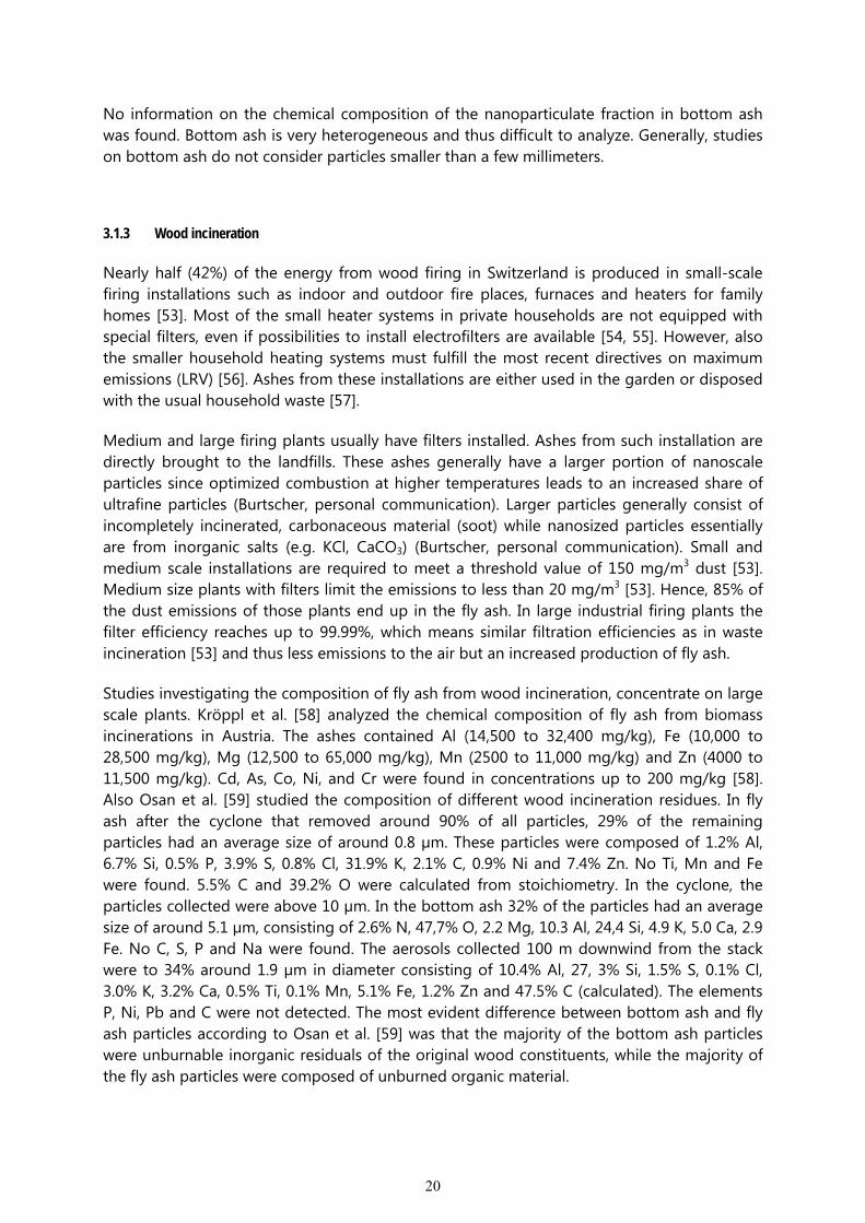
Also Pedersen et al. [49] found a bimodal size distribution (measured by laser diffraction) of the particle number in fly ash from a Danish waste incineration plant. The peaks were identified at less than 5-10 µm and at 100µm. About 10 % of all particles had a mean diameter of 1.9 µm +/- 1.0 [49]. Chen et al. observed the copper speciation in a Taiwanese WIP and found that about 24 % of the copper in the fly ash was nano-sized [50]. The particle size distribution of the smallest fly ash fraction from a municipal waste incineration in South Korea showed a peak at a mean diameter of 0.3 +/- 0.2 µm [51]. Romero et al. [52] measured the size distribution of fly ash, however focusing on particles larger than 1 µm (Fig. 11).

Fig. 11: Density of distribution (—) and particle size distribution % (- - -) for a fly ash residue mixture from a Spanish waste incinerator.

20

No information on the chemical composition of the nanoparticulate fraction in bottom ash was found. Bottom ash is very heterogeneous and thus difficult to analyze. Generally, studies on bottom ash do not consider particles smaller than a few millimeters.

 

3.1.3 Wood incineration

Nearly half (42%) of the energy from wood firing in Switzerland is produced in small-scale firing installations such as indoor and outdoor fire places, furnaces and heaters for family homes [53]. Most of the small heater systems in private households are not equipped with special filters, even if possibilities to install electrofilters are available [54, 55]. However, also the smaller household heating systems must fulfill the most recent directives on maximum emissions (LRV) [56]. Ashes from these installations are either used in the garden or disposed with the usual household waste [57].

Medium and large firing plants usually have filters installed. Ashes from such installation are directly brought to the landfills. These ashes generally have a larger portion of nanoscale particles since optimized combustion at higher temperatures leads to an increased share of ultrafine particles (Burtscher, personal communication). Larger particles generally consist of incompletely incinerated, carbonaceous material (soot) while nanosized particles essentially are from inorganic salts (e.g. KCl, CaCO3) (Burtscher, personal communication). Small and medium scale installations are required to meet a threshold value of 150 mg/m3 dust [53]. Medium size plants with filters limit the emissions to less than 20 mg/m3 [53]. Hence, 85% of the dust emissions of those plants end up in the fly ash. In large industrial firing plants the filter efficiency reaches up to 99.99%, which means similar filtration efficiencies as in waste incineration [53] and thus less emissions to the air but an increased production of fly ash.

Studies investigating the composition of fly ash from wood incineration, concentrate on large scale plants. Kröppl et al. [58] analyzed the chemical composition of fly ash from biomass incinerations in Austria. The ashes contained Al (14,500 to 32,400 mg/kg), Fe (10,000 to 28,500 mg/kg), Mg (12,500 to 65,000 mg/kg), Mn (2500 to 11,000 mg/kg) and Zn (4000 to 11,500 mg/kg). Cd, As, Co, Ni, and Cr were found in concentrations up to 200 mg/kg [58]. Also Osan et al. [59] studied the composition of different wood incineration residues. In fly ash after the cyclone that removed around 90% of all particles, 29% of the remaining particles had an average size of around 0.8 µm. These particles were composed of 1.2% Al, 6.7% Si, 0.5% P, 3.9% S, 0.8% Cl, 31.9% K, 2.1% C, 0.9% Ni and 7.4% Zn. No Ti, Mn and Fe were found. 5.5% C and 39.2% O were calculated from stoichiometry. In the cyclone, the particles collected were above 10 µm. In the bottom ash 32% of the particles had an average size of around 5.1 µm, consisting of 2.6% N, 47,7% O, 2.2 Mg, 10.3 Al, 24,4 Si, 4.9 K, 5.0 Ca, 2.9 Fe. No C, S, P and Na were found. The aerosols collected 100 m downwind from the stack were to 34% around 1.9 µm in diameter consisting of 10.4% Al, 27, 3% Si, 1.5% S, 0.1% Cl, 3.0% K, 3.2% Ca, 0.5% Ti, 0.1% Mn, 5.1% Fe, 1.2% Zn and 47.5% C (calculated). The elements P, Ni, Pb and C were not detected. The most evident difference between bottom ash and fly ash particles according to Osan et al. [59] was that the majority of the bottom ash particles were unburnable inorganic residuals of the original wood constituents, while the majority of the fly ash particles were composed of unburned organic material.

21

Pöykio et al. [60] determined the enrichment factor (EF= total element concentration in the cyclone fly ash divided by the total element concentration in the bottom ash) for several elements. He found Pb (2.6), Zn (3.8), Ba (1.9) and S (10) to be enriched in fly ash while As (0.3) and Ti (0.2) were enriched in bottom ash. Cr (0.9), Mn (1.3), Cu (1.0), Co (1.2), V (0.9), Ni (1.0) and Fe (0.8) showed no significant differences in distribution, into the two ash fractions. He found 3.6 g Zn per kg of fly ash and 0.25 g Ti per kg fly ash. Lanzerstorfer [61] determined the chemical composition of the finest fly ash fraction from wood incineration. This fraction had a Sauter diameter (Diameter of a sphere that has the same volume/surface area ratio as the particle of interest.) of 2.19 µm (determined by laser particle sizer) and summed up to 11.6% of the total weight. The following elements were found 19.4 ppm As, 29.9 ppm Cd, 16.1 ppm Co, 176 ppm Cu, 161 ppm Pb, 3680 ppm Zn as well as 17.8% Ca, 0.8% K and 0.2% Mg [61].

Dahl et al. [62] found more than 90% of the mass loadings of heavy metals from wood incineration in the finest fraction of fly ash (<74 µm) whereas in the bottom ash 84-92% were found in the fraction between 0.5-2 mm. However, in the bottom ash no particles were found below 74 µm, whereas 91 wt% of the particles in fly ash occurred in the size fraction below 74 µm. Zinc was found to be dominant in the finest fly ash fraction with 500 mg Zn per kg of fly ash.

Ronkkomaki et al. [63] reported that all fly ash particles collected from a wood incineration plant were smaller than 0.25 mm in diameter and 88.4 wt% smaller than 75 µm. This fraction also accounted for the highest concentration (89-94%) of all zinc, copper, lead, cadmium and molybdenum [63].

3.1.4 Sludge incineration

Studies on the composition of residues from sludge incineration are found mainly in context with glass ceramic and cement production processes. However, no information was found on the size distribution of the respective fly ashes. Mono-incineration of sludge is not an as wide spread technique as waste incineration. In most countries, sludge is used as fertilizer in agriculture (e.g. in Germany 2010: 46.8% [27]) or otherwise burnt in waste incinerators or cement factories. Separate combustion of sludge as it will be state of the art in Switzerland from around 2020, is rare.

3.1.5 Engineered nano-objects (ENO) in waste incineration

The increasing interest in nanotechnology and nano-enhanced products has raised concerns about the safe handling as well as human and environmental exposure. Researchers are thus investigating not only the potential toxicity of ENO but also their distribution in the environment. However, little is known about the behavior of ENO at the interface from technosphere to ecosphere. Only a few studies exist on the fate in end-of life processes of ENO which were all published only recently [64-66].

22

Besides these studies, a few research projects have been initiated targeting the end-of-life phase of ENO:

● EU Projects Prosuite (PROspective SUstaInability Assessment of Technologies, http://www.prosuite.org),

● NanoHouse (www.nanohouse.cea.fr)

● CCMX Project “NanoAir”

However, no results are available from these projects yet. On ENO in waste incineration only one experimental study is found which was published recently by Walser et al. [67]. They followed nano-CeO2 added to domestic waste during the combustion steps in a Swiss WIP. Of the total nano-CeO2 recovered, 81% were found in the slag, 19% in the fly ash and 0.02% in the quench water. Nano-CeO2 in the exhaust air was below detection limit of 0.6 ng per measurement filter. Opposite to these measurements and the measurements of Burtscher et al. [33], Roes et al. [16] claimed that the effectiveness of ESP is significantly reduced for particles < 3 µm and also in baghouse filters only 80 % of the particles are retained.

Compared to the general weight distribution bottom ash : fly ash which is in average about 9:1, the CeO2 seemed to be slightly enriched in the fly ash according to the measurements of Walser et al. [67]. This may be due to the small particle size which favors suspension in the flue gas. Moreover, the solubility of CeO2 is low especially at neutral or alkaline pHs, which makes it highly immobile for water transport. However, it partially dissolves in an acidic environment such as during acid washing of the flue gas and fly ash. Since the measurements by Walser et al. are based on chemical analysis and do not consider the morphology of the particles, it is possible that the Ce measured in the quench water is not exclusively nanoparticulate but partially dissolved.

The behavior of CeO2 during waste incineration will be comparable to the behavior of TiO2 since both substances are very stable up to high temperatures and show low solubility. However, no conclusions can be drawn from this study regarding the behavior of carbonaceous ENO and extrapolations are limited for less stable materials such as ZnO and Ag.

Based on different assumptions Roes et al. [16] calculated in a desk-top study that by 2020 about 0.5 kg of ENO in plastics are incinerated per ton of waste which would sum up to 1880 t/a of ENO entering waste incineration in Switzerland as nano-composites. Taking into account the density and the volume of the ENO they find that 100-10’000 times higher concentrations of nano-objects will be found in the flue gas of nanocomposite containing waste than produced by conventional waste. Basis for this comparison is the measured particle concentration in the exhaust (after a high efficiency cyclone) of an experimental waste incinerator using a “refuse derived fuel”. The concentration was measured at 7.52E11 particles/m3 [36]. Taking into account the flue gas produced per ton of waste incinerated, Roes et al. calculated that 3.76x1015 nano-objects are produced per ton of conventional waste while up to 9.72x1023 ENO (Fullerenes) additionally originate from nano-composites. However, Roes et al. assume that no ENO are destroyed and that all ENO end up in the flue gas.

23

Theoretical considerations show that the fate of an ENO in waste incineration depends mainly on two factors:

1. Surrounding materials: If the ENO is free or released easily from its substrate, it can escape with the flue gas, because of its small size, and finally be caught in the flue gas filter (bag filter or electrostatic filter). If the ENO is enclosed in other materials, it may be fused-in in the melts of the surrounding material and hence remain in the bottom ash.

2. Melting/boiling point: If the ENO has a boiling point lower or equal to the temperature in the incineration furnace, it will vaporize based on its small size and hence enter the flue gas stream as gaseous element. As the flue gas cools down, these elements condensate, however, they are not considered as ENO anymore. Analogously, melted ENO are unlikely to reform a nanoparticle in original composition. Very stable ENO (like TiO2 or CeO2) may remain particulate, other ENO such as carbonaceous materials are oxidized (based on the conditions in the furnace).

Based on these considerations, the fate of the most common ENO is expected as follows. Nano-TiO2 (boiling point: 2900°C) will most probably remain particulate while the majority of CNT are burnt. Nano-Ag (boiling point: 2162°C) will only volatilize to a small extent. However, nano-Ag particles are likely to melt (melting point: 962°C). The fate of nano-ZnO is difficult to predict. Sorum et al. found 37–86 wt% of Zn remaining in bottom ash [68]. This high variability depended on the redox-conditions in the furnace. In thermal waste incineration Zn starts vaporizing at a temperature of 905° C and at 1150° more than 90% is gaseous in reducing conditions [40]. However, under oxidizing conditions ZnO remains solid as ZnO up to a temperature of 1500°C [40]. In waste incineration we are expecting oxidizing conditions and therefore nano-ZnO should not vaporize to a significant extent.

 

3.2 Characterisation of pigments (TiO2, SiO2, ZnO, carbon black) regarding their share of nanosized particles

BDNO probably follow similar release patterns and pathways as ENO. But their flows to the environment have so far received almost no attention. However, according to the most recent European Commission recommendation from 18 October 2011 on the definition of nanomaterial (2011/696/EU) [69] it is proposed: “A nanomaterial as defined in this recommendation should consist for 50 % or more of particles having a size between 1 - 100 nm.” Since also pigments are probably constantly optimized regarding their functionality and properties (e.g. transparency), it was recently suspected that the size distribution of currently used pigments (e.g. in food, paints, coatings, polymers) might have a substantial size fraction below 100 nm. However, systematic studies focusing on this issue are not available yet. Also from product descriptions and data sheets of materials the information about the nano-sized fraction of pigments is usually not available.

Nonetheless, the magnitude of BDNO might be significantly higher compared to ENO. A study by Dupont shows that regular TiO2 has a small fraction of nanosized particles [70], but the amount of this portion has not been quantified. In a product information sheet, Dupont indicates the Median Particle Size of the anatase phase ranges between 0.31–0.60 μm and for

24

the rutile product at about 0.385 μm [71]. For other products a share of 0-5% nanosized TiO2 was declared (personal communication Sachtleben).

 

  

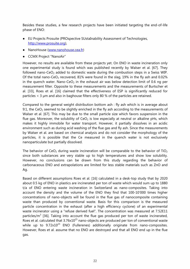
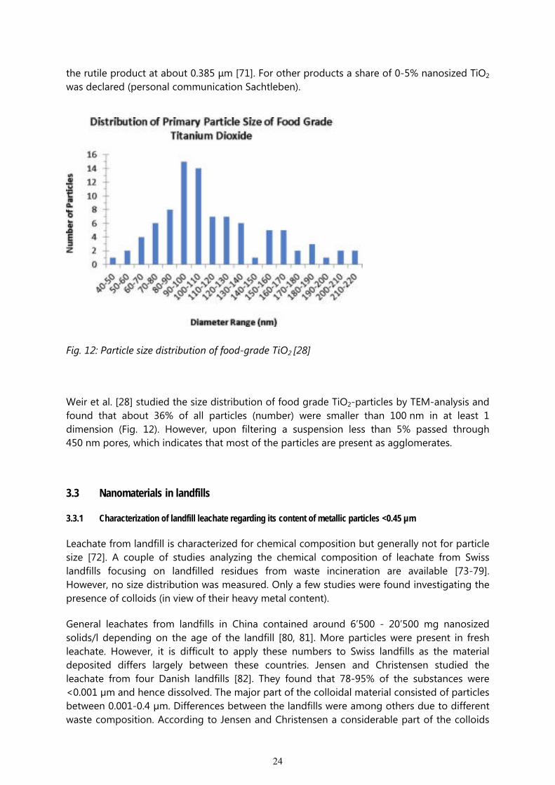
Fig. 12: Particle size distribution of food-grade TiO2 [28]

Weir et al. [28] studied the size distribution of food grade TiO2-particles by TEM-analysis and found that about 36% of all particles (number) were smaller than 100 nm in at least 1 dimension (Fig. 12). However, upon filtering a suspension less than 5% passed through 450 nm pores, which indicates that most of the particles are present as agglomerates.

 

3.3 Nanomaterials in landfills

3.3.1 Characterization of landfill leachate regarding its content of metallic particles <0.45 µm

Leachate from landfill is characterized for chemical composition but generally not for particle size [72]. A couple of studies analyzing the chemical composition of leachate from Swiss landfills focusing on landfilled residues from waste incineration are available [73-79]. However, no size distribution was measured. Only a few studies were found investigating the presence of colloids (in view of their heavy metal content).

General leachates from landfills in China contained around 6’500 - 20’500 mg nanosized solids/l depending on the age of the landfill [80, 81]. More particles were present in fresh leachate. However, it is difficult to apply these numbers to Swiss landfills as the material deposited differs largely between these countries. Jensen and Christensen studied the leachate from four Danish landfills [82]. They found that 78-95% of the substances were <0.001 µm and hence dissolved. The major part of the colloidal material consisted of particles between 0.001-0.4 µm. Differences between the landfills were among others due to different waste composition. According to Jensen and Christensen a considerable part of the colloids

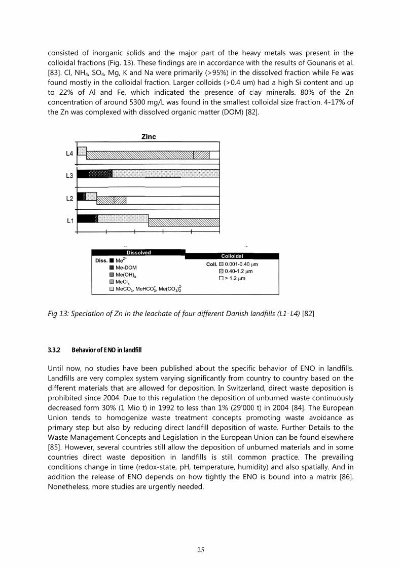
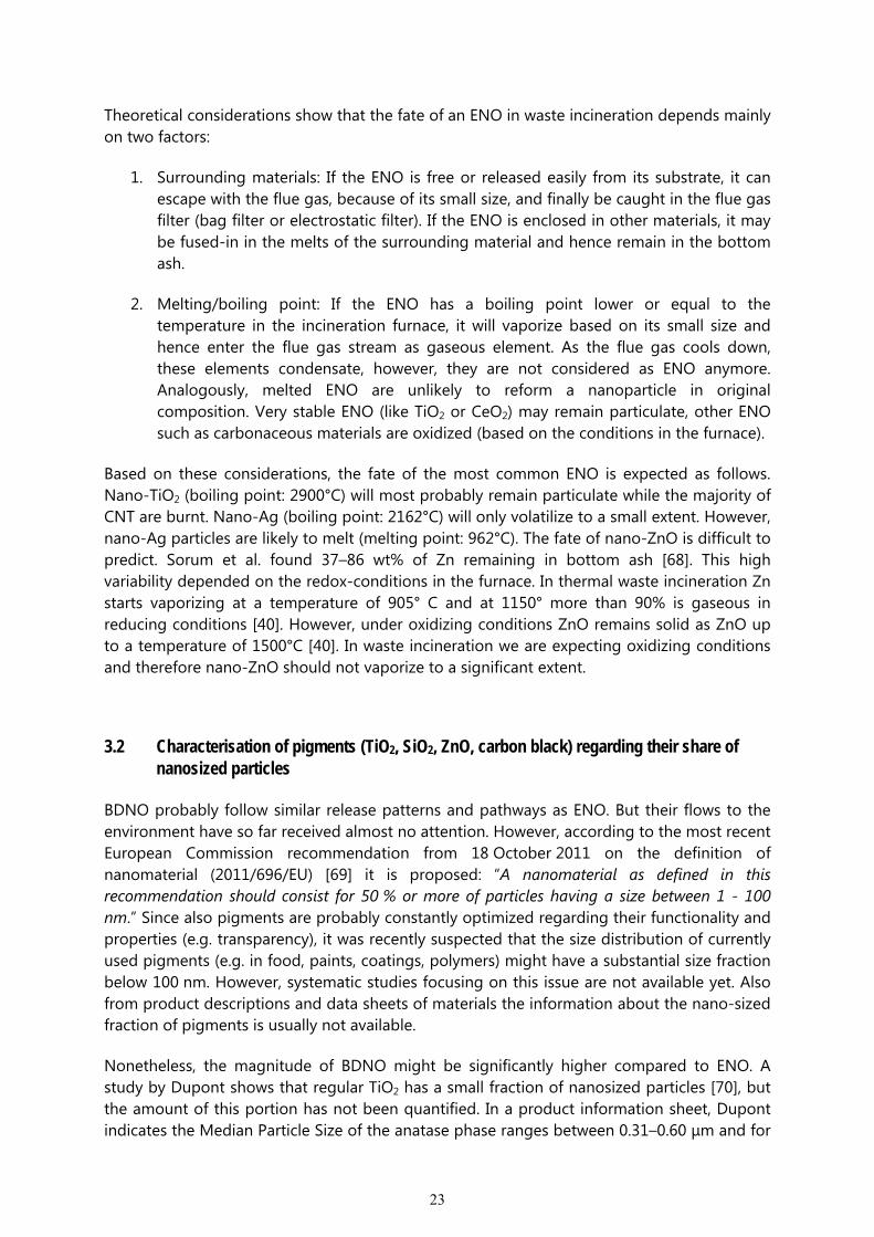
consistecolloida[83]. Cl, found mto 22%concentthe Zn w

 

 

Fig 13: S

3.3.2 B

Until noLandfillsdifferenprohibitdecreasUnion tprimaryWaste M[85]. HocountrieconditioadditionNoneth

ed of inorgal fractions (

NH4, SO4, Mmostly in th

% of Al andtration of arwas comple

Speciation o

Behavior of EN

ow, no studs are very c

nt materials ted since 20sed form 30tends to h

y step but aManagemenowever, sevees direct wons change n the releaseless, more

ganic solids (Fig. 13). ThMg, K and Ne colloidal fd Fe, whicround 5300exed with di

of Zn in the

NO in landfill

dies have bcomplex sys

that are al004. Due to0% (1 Mio thomogenizealso by redunt Conceptseral countriwaste depoin time (re

se of ENO e studies are

and the mese findingNa were prifraction. Lar

ch indicated mg/L was fssolved org

leachate of

een publishstem varyinglowed for d

o this regula) in 1992 toe waste treucing directs and Legisles still allowosition in dox-state, pdepends o

e urgently n

25

major part s are in accimarily (>95rger colloidd the presfound in th

ganic matte

four differe

hed about g significandeposition. ation the deo less than eatment cot landfill deation in thew the depolandfills is pH, temperan how tigh

needed.

of the heaordance wit5%) in the ds (>0.4 um)

sence of cle smallest cr (DOM) [82

nt Danish la

the specifictly from coIn Switzerla

eposition of1% (29’000

oncepts proeposition ofe European sition of un

still commature, humi

htly the ENO

vy metals wth the resuldissolved fra) had a highay mineral

colloidal size2].

andfills (L1-

c behavior untry to coand, direct wf unburned 0 t) in 2004 omoting wf waste. FurUnion can b

nburned mamon practidity) and a

O is bound

was presents of Gounaaction whileh Si contentls. 80% of e fraction. 4

L4) [82]

of ENO in ountry basedwaste depowaste cont[84]. The E

waste avoidrther Detailbe found el

aterials and ice. The plso spatially into a ma

 

nt in the aris et al. e Fe was t and up

the Zn 4-17% of

landfills. d on the osition is tinuously uropean ance as ls to the sewhere in some revailing y. And in trix [86].

26

4 Particle size distribution of fly ashes and pigments

The aim of the following measurements was to get an idea of the size distribution of fly ash and conventional pigments. The focus is laid on particles smaller than 100 nm. The quantification of this fraction on a mass-basis is needed to estimate the contribution of ENO, BDNO and CGNO respectively. To cover the broad size spectrum of fly ash different measurement methods had to be combined.

4.1 Sample description

4.1.1 Fly Ashes

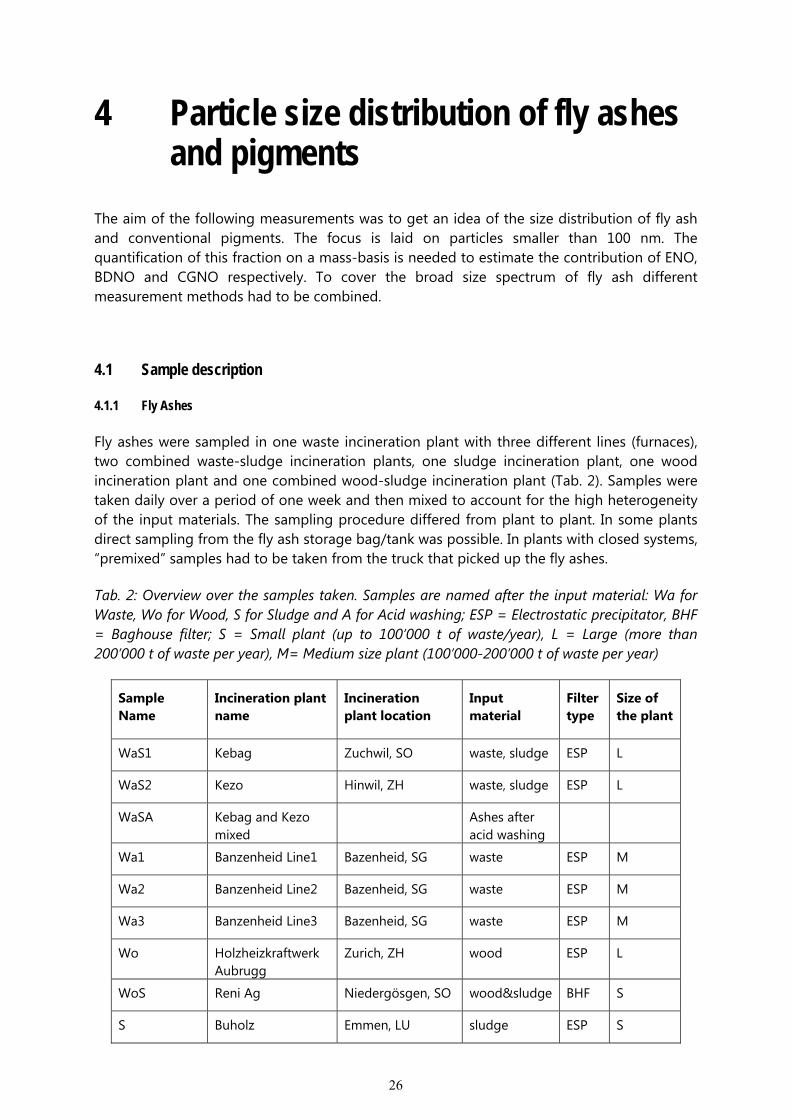
Fly ashes were sampled in one waste incineration plant with three different lines (furnaces), two combined waste-sludge incineration plants, one sludge incineration plant, one wood incineration plant and one combined wood-sludge incineration plant (Tab. 2). Samples were taken daily over a period of one week and then mixed to account for the high heterogeneity of the input materials. The sampling procedure differed from plant to plant. In some plants direct sampling from the fly ash storage bag/tank was possible. In plants with closed systems, “premixed” samples had to be taken from the truck that picked up the fly ashes.

Tab. 2: Overview over the samples taken. Samples are named after the input material: Wa for Waste, Wo for Wood, S for Sludge and A for Acid washing; ESP = Electrostatic precipitator, BHF = Baghouse filter; S = Small plant (up to 100’000 t of waste/year), L = Large (more than 200’000 t of waste per year), M= Medium size plant (100’000-200’000 t of waste per year)

Sample Name

Incineration plant name

Incineration plant location

Input material

Filter type

Size of the plant

WaS1 Kebag Zuchwil, SO waste, sludge ESP L

WaS2 Kezo Hinwil, ZH waste, sludge ESP L

WaSA Kebag and Kezo mixed

Ashes after acid washing

Wa1 Banzenheid Line1 Bazenheid, SG waste ESP M

Wa2 Banzenheid Line2 Bazenheid, SG waste ESP M

Wa3 Banzenheid Line3 Bazenheid, SG waste ESP M

Wo Holzheizkraftwerk Aubrugg

Zurich, ZH wood ESP L

WoS Reni Ag Niedergösgen, SO wood&sludge BHF S

S Buholz Emmen, LU sludge ESP S

27

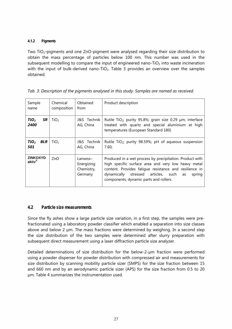
4.1.2 Pigments

Two TiO2-pigments and one ZnO-pigment were analysed regarding their size distribution to obtain the mass percentage of particles below 100 nm. This number was used in the subsequent modelling to compare the input of engineered nano-TiO2 into waste incineration with the input of bulk-derived nano-TiO2. Table 3 provides an overview over the samples obtained.

Tab. 3: Description of the pigments analysed in this study. Samples are named as received.

Sample name

Chemical composition

Obtained from

Product description

TiO2 SR 2400

TiO2 J&S Technik AG, China

Rutile TiO2; purity 95.8%; grain size 0.29 µm; interface treated with quartz and special aluminium at high temperatures (European Standard 180)

TiO2 BLR 501

TiO2 J&S Technik AG, China

Rutile TiO2; purity 98.59%; pH of aqueous suspension 7.60;

ZINKOXYD aktiv®

ZnO Lanxess–Energizing Chemistry, Germany

Produced in a wet process by precipitation. Product with high specific surface area and very low heavy metal content. Provides fatigue resistance and resilience in dynamically stressed articles, such as spring components, dynamic parts and rollers.

4.2 Particle size measurements

Since the fly ashes show a large particle size variation, in a first step, the samples were pre-fractionated using a laboratory powder classifier which enabled a separation into size classes above and below 2 µm. The mass fractions were determined by weighing. In a second step the size distribution of the two samples were determined after slurry preparation with subsequent direct measurement using a laser diffraction particle size analyzer.

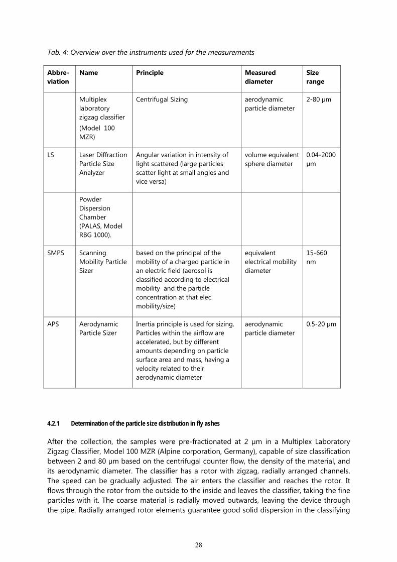
Detailed determinations of size distribution for the below-2-µm fraction were performed using a powder disperser for powder distribution with compressed air and measurements for size distribution by scanning mobility particle sizer (SMPS) for the size fraction between 15 and 660 nm and by an aerodynamic particle sizer (APS) for the size fraction from 0.5 to 20 µm. Table 4 summarizes the instrumentation used.

28

Tab. 4: Overview over the instruments used for the measurements

Abbre-viation

Name Principle Measured diameter

Size range

Multiplex laboratory zigzag classifier (Model 100 MZR)

Centrifugal Sizing aerodynamic particle diameter

2-80 µm

LS Laser Diffraction Particle Size Analyzer

Angular variation in intensity of light scattered (large particles scatter light at small angles and vice versa)

volume equivalent sphere diameter

0.04-2000 µm

Powder Dispersion Chamber (PALAS, Model RBG 1000).

SMPS Scanning Mobility Particle Sizer

based on the principal of the mobility of a charged particle in an electric field (aerosol is classified according to electrical mobility and the particle concentration at that elec. mobility/size)

equivalent electrical mobility diameter

15-660 nm

APS Aerodynamic Particle Sizer

Inertia principle is used for sizing. Particles within the airflow are accelerated, but by different amounts depending on particle surface area and mass, having a velocity related to their aerodynamic diameter

aerodynamic particle diameter

0.5-20 µm

4.2.1 Determination of the particle size distribution in fly ashes

After the collection, the samples were pre-fractionated at 2 µm in a Multiplex Laboratory Zigzag Classifier, Model 100 MZR (Alpine corporation, Germany), capable of size classification between 2 and 80 µm based on the centrifugal counter flow, the density of the material, and its aerodynamic diameter. The classifier has a rotor with zigzag, radially arranged channels. The speed can be gradually adjusted. The air enters the classifier and reaches the rotor. It flows through the rotor from the outside to the inside and leaves the classifier, taking the fine particles with it. The coarse material is radially moved outwards, leaving the device through the pipe. Radially arranged rotor elements guarantee good solid dispersion in the classifying

29

air. The variation of the desired cut size is performed by varying the speed of rotation and the air throughput on the basis of an empiric calibration curve. Before and after the pre-fractionation a Laser Diffraction Particle Size Analyser (LS 230) was used to determine the size distribution of the samples. Therefore, small sample amounts were used to prepare a slurry before the sample was directly measured with the LDPSA. By this analysis we could get an overall idea of the fractionation quality, as well as the mass percentage of the fraction below 2 µm. The mass of all fly ash samples was also measured before and after the pre-fractionation. Based on these measurements sample loss as well as the mass percentage of both fractions was calculated.

In the second step, the fractions below 2 µm were aerosolized in a Powder Dispersion Chamber (PALAS, Model RBG 1000). Each experiment was conducted following the same procedure. First the flow of the compressed air in the powder dispersion chamber was turned on to clean the background air while measuring the particle concentrations in the chamber by the APS (Aerodynamic Particle Sizer, TSI, Model 3321) and SMPS (Scanning Mobility Particle Sizer). This lasted until the background total number concentration was less than 500 particles per cm3. If necessary the brush from the dispersion chamber (used to disperse and aerosolize the material) and the tubing system was additionally cleaned with the back pulse. After checking the background number concentrations, material of interest was placed in the disperser, and with the controlled air flow (compressed air, pressure at 1 bar, which is equivalent to 1.25 m3/h flow rate), as well as the brush (940 rpm) and dispersion speed (50 mm/h), the size distribution from the chamber was directly measured.

Due to the high concentrations a diluter was used and the flow controller, varying the dilution ratio in order to get the most reliable results and to stay within the detection limits for both of the instruments. The best results of the total concentration of the aerosolized samples were obtained when dilution was 1:3 in case of SMPS and 1:10 for the APS measurements. The samples were aerosolized by introducing compressed air at a flow rate high enough to disperse the particles in air and bring them to the measurement instruments. Size distribution measurements were carried out with SMPS measuring the range from 14.6 to 661.2 nm and APS which covered the size range from 0.5 to 20 µm.

In the size distribution measurement using Scanning Mobility Particle Sizer (SMPS), the particles are represented by their equivalent electrical mobility diameter, which is the diameter for spheres which possess the same electrical mobility as the measured particles. SMPS is consisting of a DMA (Differential Mobility Analyzer, TSI, Model 3081) that is selecting certain mobility diameter size and a CPC (Condensation Particle Counter, TSI, Model 3775) that is counting the number of particles of that particular size. SMPS typically requires a measurement time of a couple of minutes and provides size distribution curves in the range below 1 μm, with higher precision than data received from the other electrical mobility instruments with 1 s time resolution, such as Fast Mobility Particle Sizer (FMPS) etc. APS provides particle number distribution as a function of their aerodynamic particle diameter. By merging these two distributions and comparing them with the Laser Diffraction Particle Size Analyser (LS 230) measurements for the overall overview, respective number and mass percentage of the different size fractions are calculated.

This experimental set-up allowed us to measure the number concentrations directly without assuming the shape of the particle size distribution. It has a high degree of absolute sizing accuracy and measurement repeatability with broad size and concentration ranges being

30

covered. It further allows determining the mass percentage of particles below 100 nm, which was the main interest of this study. However, since SMPS and APS are based on different working principles the obtained data had to be merged by calculations that take into account the fundamental physical principles [87]. Given two concurrently measured SMPS and APS spectra, equations Eq. (1) and Eq. (2) show how to commonly transform aerodynamic diameter Da to mobility diameter Dp.

Eq. (1)

where C is the Cunningham slip correction factor and where the number parameter x is given by:

∗ Eq. (2)

where ρ0 is unit density (1.0g/cm3), ρe is the density of the material and λ is the shape factor.

Based on the testing material and information from literature, the number parameter x (Eq. (2)) was calculated and fixed, and not left as free parameter as in previous studies [88, 89]. Since the dilution ratio for SMPS and APS were different, the transition region matching factor, δ, is introduced instead.

General merging procedures of SMPS and APS spectrums reported so far were based on different assumptions, such as: constant size correction factor [89], transition regime mobility density [90], constant shape factor over the narrow region of overlap [91], the combination of GMD (geometric mean diameter), N (number concentration) and GSD (geometric standard deviation) of different modes [92]. There are some publications where merging was applied, but not explained [93] or where the geometric diameter for all of the APS channels was calculated and particle density estimated accordingly, in the overlapping regime [94].

The procedure we have used was initialized by increasing the transition region matching factor (δ) from factor 1, when there was no correction, to extension or overlap, when correction was applied. In the case of fly ashes the number parameter (Eq.2) was less than 1, so the Da values are converted to larger values of Dp. It is thus possible that there is no overlap between the SMPS and APS spectra. In this case, the SMPS curve was extended and matched to the APS curve by choosing a proper value of δ. In case of commercially available pigments this parameter was more than 1, bringing up the overlap of the spectra instead. For this purpose equal steps in the value of δ were used, after which a more accurate optimum value δ is found through further iterations. The difference in the transition region behaviour had mostly to do with the difference in the density of the material and the respective shape factor. If those parameters led to conversion from an aerodynamic diameter to a mobility diameter with a smaller value, there were more matching points for the SMPS and APS spectra and vice versus. The transition region matching factor is introduced for the first time to our knowledge.

This approach was used to merge APS spectrum to its counterpart SMPS spectrum. For a calculated and fixed number parameter x, Dp is numerically calculated from Da for all aerodynamic diameter bins of the APS spectrum. Density and shape factor were fixed and used for the further calculation. Transition region matching factor (δ) was the main variable being optimized, using equal steps in the value, and taking in consideration the dilution ratio

31

difference between the two instruments. For each value used, aerodynamic diameters are first modified and after converted to dA/dlogDp vs. Dp and dV/dlogDp vs. Dp representations, using Eq. (3) and Eq. (4) [95]. The dN/dlogDP distribution was normalized by the size of the bin to avoid distortion caused by different bin sizes. Through a number of iterations an optimum value of δ was chosen which led to the best transition for all three distribution curves (dN, dA and dV).

Eq. (3)

Eq. (4)

The physical and chemical parameters to characterize fly ashes are specific gravity, grain size, compaction characteristics, permeability coefficient, shear strength parameters and consolidation parameters [47]. The properties of ash are a function of several variables such as source, degree of pulverization, design of boiler unit, loading and firing conditions, handling and storage methods. A change in any of the above factors can result in detectable changes in the properties of the ash produced explaining the differences found between the samples. Density of the fly ashes is usually below the unit density. The average value for density was considered as the average from the literature available (0.8 g/cm3), and the same was done for the shape factor (1.25) [96]. The number parameter x was calculated following Eq. (2) and fixed. The free transition region matching factor, δ, was fitted according to the matching extension.

As reported in previous studies, some additional merging procedures were applied. A drop of efficiency has been reported for the APS size bins measuring particles with aerodynamic diameters below 0.7 µm, i.e., the first four size bins of the APS. Those size bins to the lower particle side of the peak are omitted and those to the other side of the peak are used to fit the APS spectrum to the SMPS spectrum. [40]. The APS data points were fitted to SMPS data, resulting in the optimum fit shown by continuous transition.

4.2.2 Determination of the particle size distribution in commercial pigments

The size distribution of the pigments was determined using similar methods as for the fly ashes. However, pre-fractionation of the pigment samples was not necessary due to the homogeneity and the smaller size distribution of the material. Hence, the samples were used as received. They were directly aerosolized and further analysed with the SMPS and APS set-up as previously described.

Unlike for fly ashes, the densities of TiO2 and ZnO are well known (4.2 g/cm3 and 5.6 g/cm3 respectively; shape factor=1.08 for both materials [96]), and additionally confirmed by the companies producing these pigments, from which the investigated powders were provided. Higher density of the material made x>1 (Eq.2) and Da is converted to a Dp of smaller value. Thus SMPS and APS spectrums are ensured to have an overlapping region. Through number of iterations an optimum was chosen. For each value used, aerodynamic diameters are first modified and after converted to dA/dlogDp vs. Dp and dV/dlogDp vs. Dp representations, using Eq. (3) and Eq. (4).

32

The APS data points were fitted to SMPS data, resulting in the optimum fit shown by overlapping in case of pigments.

4.3 Results

4.3.1 Size distribution of fly ashes from waste, sludge and wood incineration plants

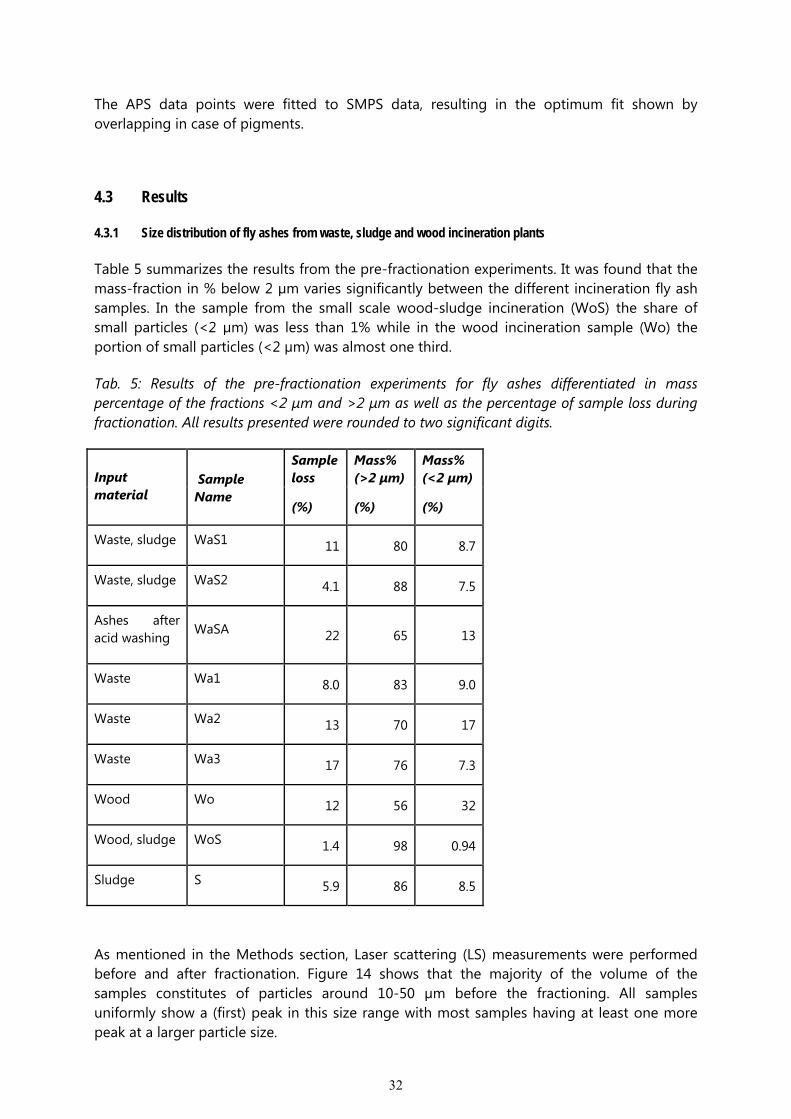
Table 5 summarizes the results from the pre-fractionation experiments. It was found that the mass-fraction in % below 2 µm varies significantly between the different incineration fly ash samples. In the sample from the small scale wood-sludge incineration (WoS) the share of small particles (<2 µm) was less than 1% while in the wood incineration sample (Wo) the portion of small particles (<2 µm) was almost one third.

Tab. 5: Results of the pre-fractionation experiments for fly ashes differentiated in mass percentage of the fractions <2 µm and >2 µm as well as the percentage of sample loss during fractionation. All results presented were rounded to two significant digits.

Input material

Sample Name

Sample loss

Mass% (>2 µm)

Mass% (<2 µm)

(%) (%) (%)

Waste, sludge WaS1 11 80 8.7

Waste, sludge WaS2 4.1 88 7.5

Ashes after acid washing

WaSA 22 65 13

Waste Wa1 8.0 83 9.0

Waste Wa2 13 70 17

Waste Wa3 17 76 7.3

Wood Wo 12 56 32

Wood, sludge WoS 1.4 98 0.94

Sludge S 5.9 86 8.5

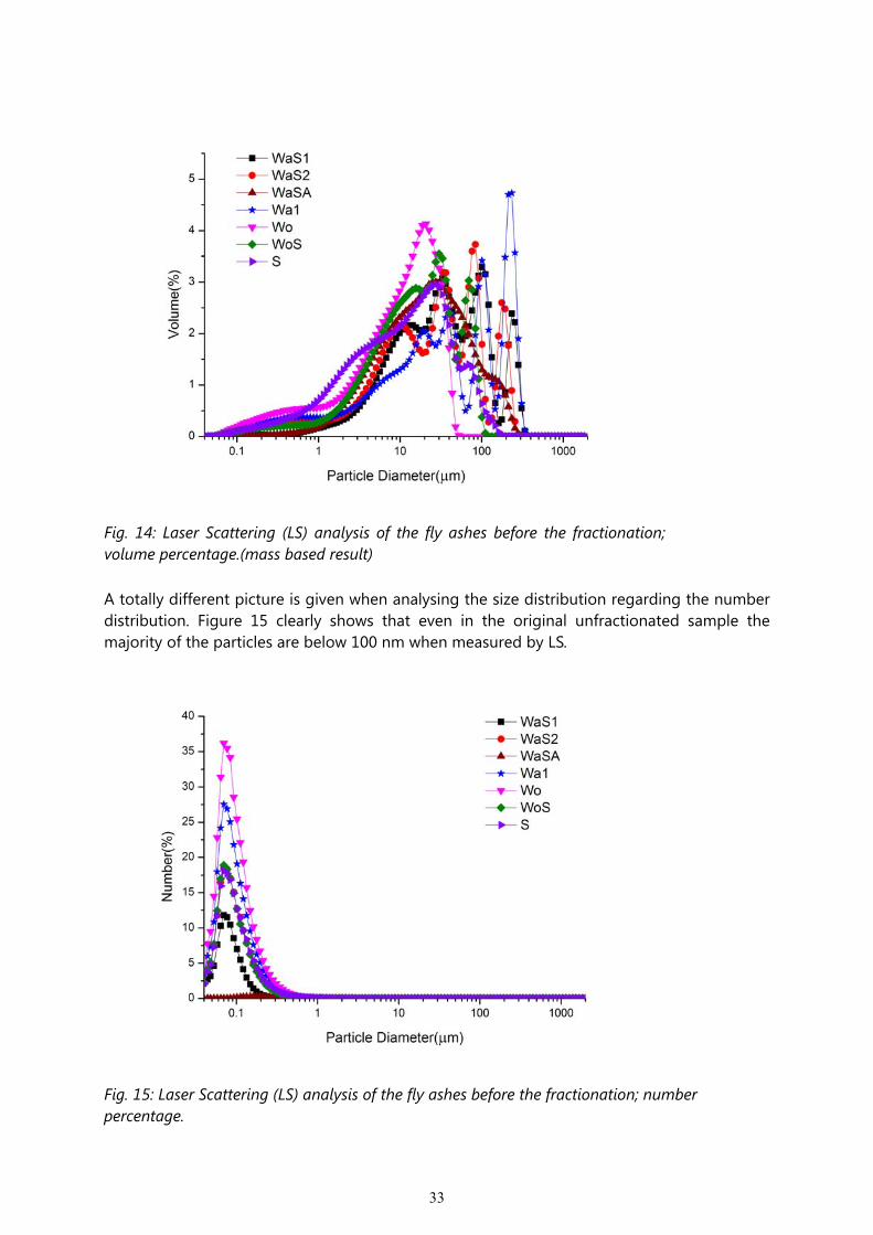
As mentioned in the Methods section, Laser scattering (LS) measurements were performed before and after fractionation. Figure 14 shows that the majority of the volume of the samples constitutes of particles around 10-50 µm before the fractioning. All samples uniformly show a (first) peak in this size range with most samples having at least one more peak at a larger particle size.

33

Fig. 14: Laser Scattering (LS) analysis of the fly ashes before the fractionation; volume percentage.(mass based result)

A totally different picture is given when analysing the size distribution regarding the number distribution. Figure 15 clearly shows that even in the original unfractionated sample the majority of the particles are below 100 nm when measured by LS.

Fig. 15: Laser Scattering (LS) analysis of the fly ashes before the fractionation; number percentage.

34

After fractionation at 2 µm, LS data proved that still particles larger than 100 nm contribute the most to the volume of the sample fractions <2 µm. A bimodal size distribution was found with peaks at around 400 nm and 2 µm. LS measurements are based on relative percentages, and after the fractionation, relative percentage changes drastically. LS also uses curve fitting to obtain size distributions, which may cause significant errors when multiple modes are present in the distribution. Since these measurements are in relative mode, additional characterization techniques were applied. Hence, all samples were further analysed with SMPS and APS techniques.

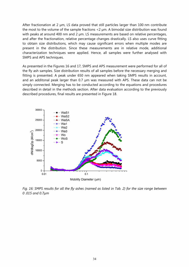
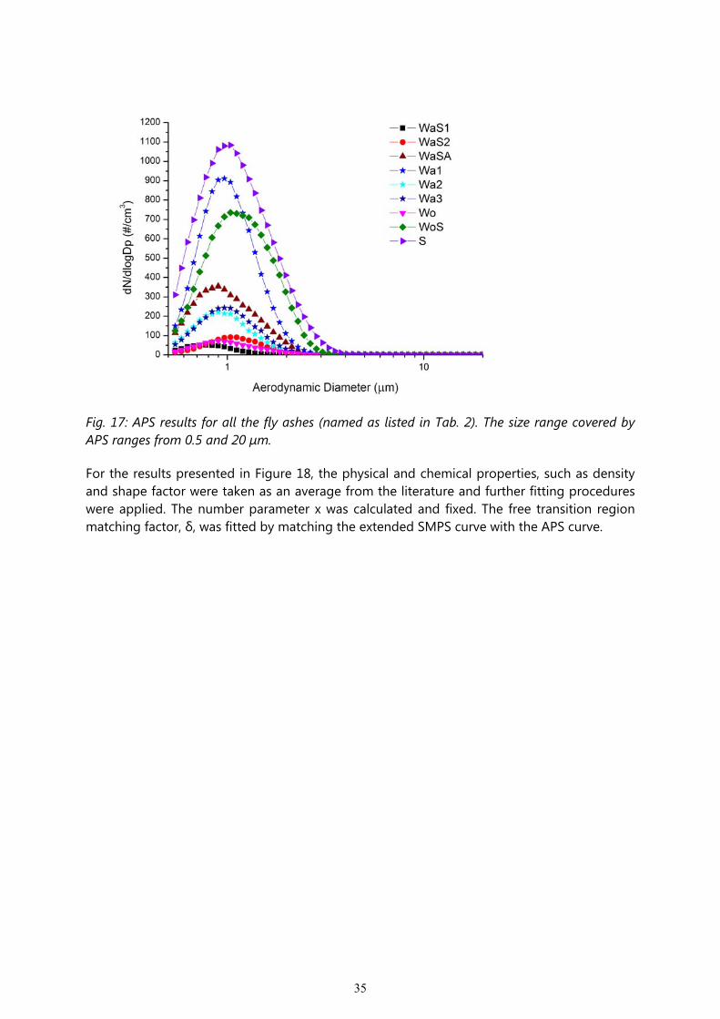
As presented in the Figures 16 and 17, SMPS and APS measurement were performed for all of the fly ash samples. Size distribution results of all samples before the necessary merging and fitting is presented. A peak under 650 nm appeared when taking SMPS results in account, and an additonal peak larger than 0.7 µm was measured with APS. These data can not be simply connected. Merging has to be conducted according to the equations and procedures described in detail in the methods section. After data evaluation according to the previously described procedures, final results are presented in Figure 18.

 

Fig. 16: SMPS results for all the fly ashes (named as listed in Tab. 2) for the size range between 0 .015 and 0.7µm

 

35

Fig. 17: APS results for all the fly ashes (named as listed in Tab. 2). The size range covered by APS ranges from 0.5 and 20 µm.

For the results presented in Figure 18, the physical and chemical properties, such as density and shape factor were taken as an average from the literature and further fitting procedures were applied. The number parameter x was calculated and fixed. The free transition region matching factor, δ, was fitted by matching the extended SMPS curve with the APS curve.

 

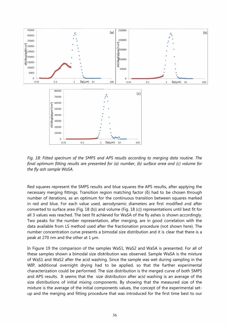
Fig. 18: final opthe fly a

Red squnecessanumberin red aconvertall 3 valTwo pedata avanumberpeak at

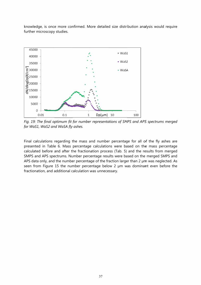
In Figurthese saof WaS1WIP, adcharacteand APSsize dismixture up and

Fitted spectimum fittin

ash sample W

uares represary mergingr of iteratioand blue. Fed to surfacues was reaaks for theailable fromr concentrat270 nm an

re 19 the coamples show1 and WaS2dditional oerization coS results. Ittributions o is the averthe mergin

ctrum of theng results aWaSA.  

sent the SMg fittings. Trns, as an o

For each vace area (Figached. The be number rem LS methotion curve pd the other

omparison wn a bimod2 after the avernight d

ould be perft seems thaof initial mrage of the ng and fittin

e SMPS andare presente

MPS results ransition reptimum for

alue used, a. 18 (b)) andbest fit achiepresentatiod used afte

presents a bat 1 µm.

of the samdal size distacid washinrying had formed. Theat the sizeixing compinitial comp

ng procedu

36

d APS resulted for (a) nu

and blue sqgion matchr the continaerodynamid volume (Fieved for Won, after mer the fractibimodal size

ples WaS1, tribution wang. Since th

to be appe size distribdistribution

ponents. Byponents valre that was

ts accordingumber, (b) s

quares the hing factor nuous transic diameter

Fig. 18 (c)) reWaSA of the merging, are

onation proe distributio

WaS2 andas observede sample wplied, so tbution is thn after acid showing tues, the co

s introduced

g to mergingurface area

APS results(δ) had to ition betwers are first epresentatiofly ashes is

e in good cocedure (noon and it is

WaSA is pd. Sample Wwas wet duri

hat the fue merged c

d washing ishat the mencept of thd for the fir

ng data routa and (c) vo

s, after applbe chosen

een squaresmodified aons until beshown acco

correlation ot shown heclear that t

presented. FWaSA is theing samplin

urther expecurve of bos an averageasured size experimerst time bes

tine. The lume for

ying the through marked nd after

est fit for ordingly. with the ere). The here is a

For all of mixture

ng in the erimental th SMPS

ge of the e of the ntal set-st to our

knowledfurther

Fig. 19: for WaS

Final capresentcalculatSMPS aAPS datseen frofraction

dge, is oncemicroscopy

The final opS1, WaS2 an

alculations red in Tableed before and APS speta only, andom Figure ation, and a

e more cony studies.

ptimum fit nd WaSA fly

regarding te 6. Mass and after thectrums. Nu the numbe15 the numadditional c

nfirmed. Mo

for numberashes.

the mass apercentagehe fractiona

umber perceer percentagmber percecalculation w

37

ore detailed

r representa

nd numbere calculationation proceentage resuge of the fra

entage belowas unnece

d size distri

ations of SM

r percentagns were baess (Tab. 5) ults were baaction large

ow 2 µm wssary.

ibution ana

MPS and APS

ge for all oased on the

and the reased on the er than 2 µmas dominan

alysis would

S spectrums

of the fly ase mass peresults from e merged SMm was neglent even be

d require

s merged

shes are rcentage merged

MPS and ected. As efore the

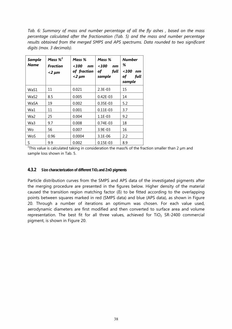
38

Tab. 6: Summary of mass and number percentage of all the fly ashes , based on the mass percentage calculated after the fractionation (Tab. 5) and the mass and number percentage results obtained from the merged SMPS and APS spectrums. Data rounded to two significant digits (max. 3 decimals).

Sample Name

Mass %1

Fraction <2 µm

Mass % <100 nm of fraction <2 µm

Mass % <100 nm of full sample

Number % <100 nm of full sample

WaS1 11 0.021 2.3E-03 15

WaS2 8.5 0.005 0.42E-03 14

WaSA 19 0.002 0.35E-03 5.2

Wa1 11 0.001 0.11E-03 3.7

Wa2 25 0.004 1.1E-03 9.2

Wa3 9.7 0.008 0.74E-03 18

Wo 56 0.007 3.9E-03 16

WoS 0.96 0.0004 3.1E-06 2.2

S 9.9 0.002 0.15E-03 8.9 1This value is calculated taking in consideration the mass% of the fraction smaller than 2 µm and sample loss shown in Tab. 5.  

4.3.2 Size characterization of different TiO2 and ZnO pigments

Particle distribution curves from the SMPS and APS data of the investigated pigments after the merging procedure are presented in the figures below. Higher density of the material caused the transition region matching factor (δ) to be fitted according to the overlapping points between squares marked in red (SMPS data) and blue (APS data), as shown in Figure 20. Through a number of iterations an optimum was chosen. For each value used, aerodynamic diameters are first modified and then converted to surface area and volume representation. The best fit for all three values, achieved for TiO2 SR-2400 commercial pigment, is shown in Figure 20.

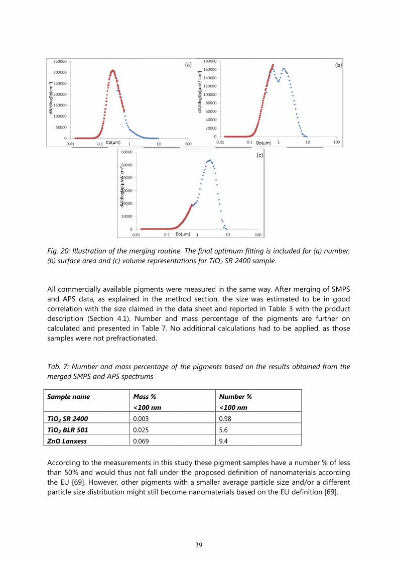
Fig. 20: (b) surfa

All comand APcorrelatdescriptcalculatsamples

Tab. 7: Nmerged

Sample

TiO2 SR

TiO2 BLR

ZnO Lan

Accordithan 50the EU particle

Illustration ace area and

mercially avS data, as

tion with thtion (Sectioed and pres were not p

Number anSMPS and A

name

2400 R 501 nxess

ng to the m0% and wou[69]. Howevsize distrib

of the mergd (c) volume

vailable pigexplained ie size claim

on 4.1). Nuesented in Tprefractiona

nd mass perAPS spectru

Mas<10

0.00

0.02

0.06

measuremenuld thus notver, other pution might

ging routinee representa

ments werein the meth

med in the dmber and

Table 7. Noated.

rcentage of ums

ss % 00 nm 03

25

69

nts in this stt fall under pigments wt still becom

39

e. The final oations for TiO

e measuredhod sectiondata sheet amass perc

o additional

the pigmen

tudy these pthe proposith a smalle

me nanomat

optimum fitO2 SR 2400

in the samn, the size and reporte

centage of calculation

nts based on

Number %<100 nm

0.98

5.6

9.4

pigment samsed definitioer average pterials base

tting is inclusample.

me way. Aftewas estimaed in Table the pigme

ns had to b

n the results

%

mples have on of nanomparticle sized on the EU

uded for (a)

er merging ated to be

3 with the ents are furbe applied,

s obtained f

a number %materials ace and/or a U definition

number,

of SMPS in good product

rther on as those

from the

% of less ccording different [69].

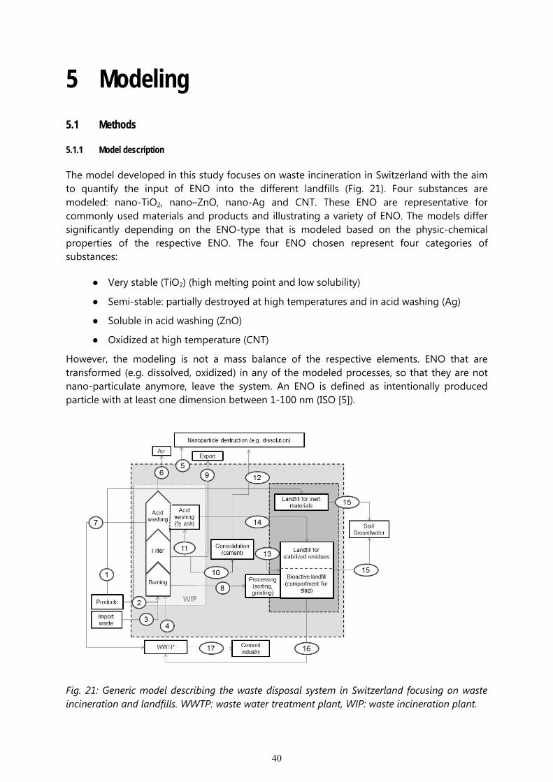
40

5 Modeling

5.1 Methods

5.1.1 Model description

The model developed in this study focuses on waste incineration in Switzerland with the aim to quantify the input of ENO into the different landfills (Fig. 21). Four substances are modeled: nano-TiO2, nano–ZnO, nano-Ag and CNT. These ENO are representative for commonly used materials and products and illustrating a variety of ENO. The models differ significantly depending on the ENO-type that is modeled based on the physic-chemical properties of the respective ENO. The four ENO chosen represent four categories of substances:

● Very stable (TiO2) (high melting point and low solubility)

● Semi-stable: partially destroyed at high temperatures and in acid washing (Ag)

● Soluble in acid washing (ZnO)

● Oxidized at high temperature (CNT)

However, the modeling is not a mass balance of the respective elements. ENO that are transformed (e.g. dissolved, oxidized) in any of the modeled processes, so that they are not nano-particulate anymore, leave the system. An ENO is defined as intentionally produced particle with at least one dimension between 1-100 nm (ISO [5]).

 

Fig. 21: Generic model describing the waste disposal system in Switzerland focusing on waste incineration and landfills. WWTP: waste water treatment plant, WIP: waste incineration plant.

41

Figure 21 illustrates the model developed for this study. There are four input flows feeding into the system (Flows 1 to 4). The first flow (1) describes the direct deposition of construction waste in landfills for inert materials. Flow 2 represents the disposal of consumer products (in Switzerland all domestic waste is burned). Flow 3 quantifies the import of waste from neighboring countries. Flow 4 represents the combustion of sewage sludge. The flows 2-4 enter the waste incineration process consisting of (A) burning under oxidizing conditions at a temperature of around 1000°C, (B) flue gas filter (either electrostatic precipitator or bag house filter depending on the incineration plant), (C) flue gas scrubber, (D) wastewater treatment facility (internal or external) for the wastewater originating from the cooling processes of the bottom ash, the wastewater from the scrubber and possibly from the acid washing of the fly ash (E). Within this waste incineration system ENO may be destroyed by oxidation, melting or volatilization in the furnace or by dissolution/precipitation in the wastewater treatment plant or in the scrubber (5). ENO that survive the waste incineration process are found in the bottom (8) as well as in fly ash (9-11) and they are released into the air (6) or into the quench water (7) wherewith they leave the system. In Switzerland bottom ash is processed on the landfill site (removal of ferrous and non-ferrous metals, grinding) before deposition in a separate compartment of the bioactive landfill (8). During grinding ENO may be released into the air. However, this potential ENO-flow is not quantified because no data is available and because it is unlikely that ENO are released in their original form. ENO in filter ash are either exported (9, leaving the system), consolidated with cement (10) or undergo acid washing (11). During both processes (consolidation, acid washing) ENO may be destroyed (1, 12). If not, they are deposited on a landfill for stabilized residues or on a bioactive landfill (13, 14). In these landfills ENO accumulate and/or leach out to the environment (15) and/or the waste water treatment plant (16). Flow 17 describes the sludge used in cement industry.

5.1.2 Model parameters (input parameters, transfer coefficients)

The input data for the flows feeding into the model were taken from Gottschalk et al. [22] (Tab. 8). Analogous average ENO-concentrations were assumed in both Swiss and imported waste. Based on the high data uncertainty three scenarios are modeled. The mode-scenario describes the values that have the highest probability. The low exposure (min) and maximum exposure (max) scenario indicate the range within which the values are to be expected (15 and 85-percentile, respectively). The input data and coefficients used in the min-scenario lead to the lowest realistic concentration of ENO in landfills, while the input data and coefficients used in the max-scenario lead to the highest realistic concentration of ENO in landfills.

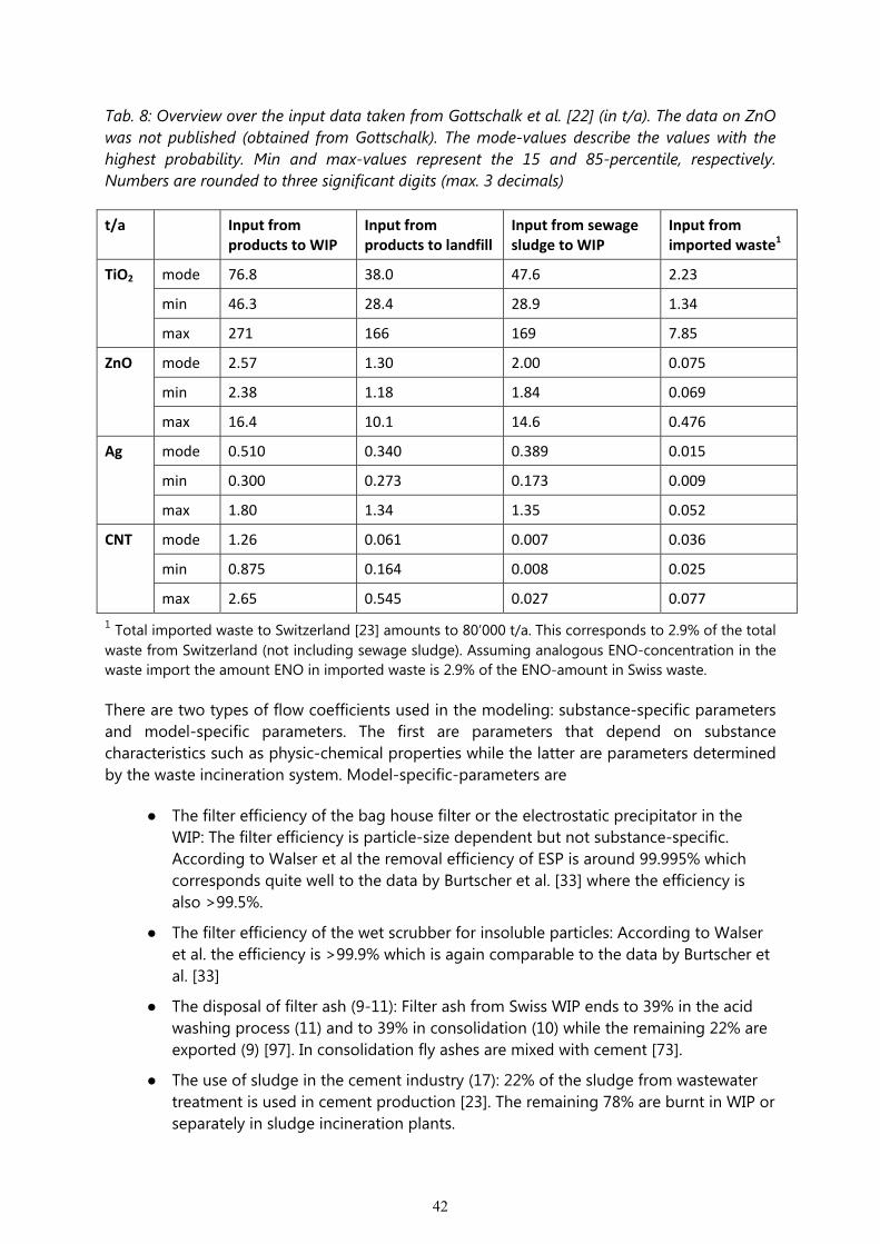
42

Tab. 8: Overview over the input data taken from Gottschalk et al. [22] (in t/a). The data on ZnO was not published (obtained from Gottschalk). The mode-values describe the values with the highest probability. Min and max-values represent the 15 and 85-percentile, respectively. Numbers are rounded to three significant digits (max. 3 decimals)

t/a    Input from products to WIP 

Input from products to landfill 

Input from sewage sludge to WIP 

Input from imported waste1 

TiO2  mode  76.8   38.0  47.6  2.23 

min  46.3  28.4  28.9  1.34 

max  271  166  169  7.85 

ZnO  mode  2.57  1.30  2.00  0.075 

min  2.38  1.18  1.84  0.069 

max  16.4  10.1  14.6  0.476 

Ag  mode  0.510  0.340  0.389  0.015 

min  0.300  0.273  0.173  0.009 

max  1.80  1.34  1.35  0.052 

CNT  mode  1.26  0.061  0.007  0.036 

min  0.875  0.164  0.008  0.025 

max  2.65  0.545  0.027  0.077 

1 Total imported waste to Switzerland [23] amounts to 80’000 t/a. This corresponds to 2.9% of the total waste from Switzerland (not including sewage sludge). Assuming analogous ENO-concentration in the waste import the amount ENO in imported waste is 2.9% of the ENO-amount in Swiss waste.

There are two types of flow coefficients used in the modeling: substance-specific parameters and model-specific parameters. The first are parameters that depend on substance characteristics such as physic-chemical properties while the latter are parameters determined by the waste incineration system. Model-specific-parameters are

● The filter efficiency of the bag house filter or the electrostatic precipitator in the WIP: The filter efficiency is particle-size dependent but not substance-specific. According to Walser et al the removal efficiency of ESP is around 99.995% which corresponds quite well to the data by Burtscher et al. [33] where the efficiency is also >99.5%.

● The filter efficiency of the wet scrubber for insoluble particles: According to Walser et al. the efficiency is >99.9% which is again comparable to the data by Burtscher et al. [33]

● The disposal of filter ash (9-11): Filter ash from Swiss WIP ends to 39% in the acid washing process (11) and to 39% in consolidation (10) while the remaining 22% are exported (9) [97]. In consolidation fly ashes are mixed with cement [73].

● The use of sludge in the cement industry (17): 22% of the sludge from wastewater treatment is used in cement production [23]. The remaining 78% are burnt in WIP or separately in sludge incineration plants.

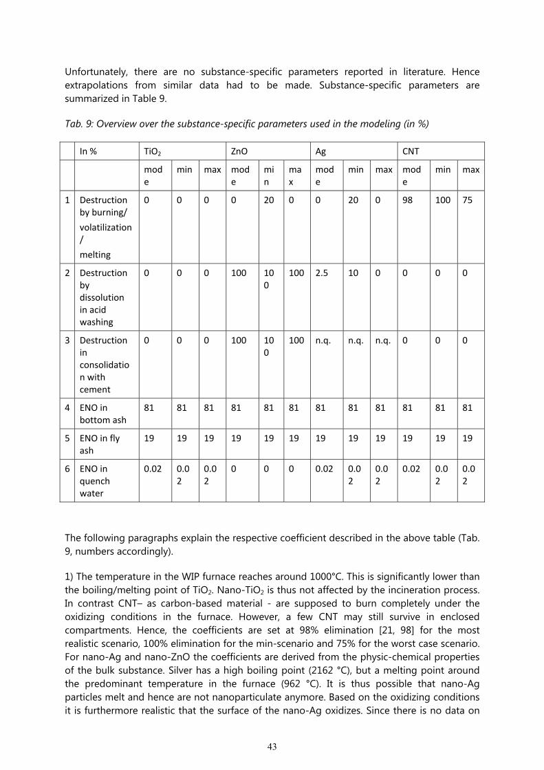
43

Unfortunately, there are no substance-specific parameters reported in literature. Hence extrapolations from similar data had to be made. Substance-specific parameters are summarized in Table 9.

Tab. 9: Overview over the substance-specific parameters used in the modeling (in %)

  In %  TiO2  ZnO  Ag  CNT 

    mode 

min  max  mode 

min 

max 

mode 

min  max  mode 

min  max

1  Destruction by burning/ 

volatilization/ 

melting 

0  0  0  0  20  0  0  20  0  98  100  75 

2  Destruction by dissolution in acid washing 

0  0  0  100  100 

100  2.5  10  0  0  0  0 

3  Destruction in consolidation with cement 

0  0  0  100  100 

100  n.q.  n.q.  n.q.  0  0  0 

4  ENO in bottom ash 

81  81  81  81  81  81  81  81  81  81  81  81 

5  ENO in fly ash 

19  19  19  19  19  19  19  19  19  19  19  19 

6  ENO in quench water 

0.02  0.02 

0.02 

0  0  0  0.02  0.02 

0.02 

0.02  0.02 

0.02 

The following paragraphs explain the respective coefficient described in the above table (Tab. 9, numbers accordingly).

1) The temperature in the WIP furnace reaches around 1000°C. This is significantly lower than the boiling/melting point of TiO2. Nano-TiO2 is thus not affected by the incineration process. In contrast CNT– as carbon-based material - are supposed to burn completely under the oxidizing conditions in the furnace. However, a few CNT may still survive in enclosed compartments. Hence, the coefficients are set at 98% elimination [21, 98] for the most realistic scenario, 100% elimination for the min-scenario and 75% for the worst case scenario. For nano-Ag and nano-ZnO the coefficients are derived from the physic-chemical properties of the bulk substance. Silver has a high boiling point (2162 °C), but a melting point around the predominant temperature in the furnace (962 °C). It is thus possible that nano-Ag particles melt and hence are not nanoparticulate anymore. Based on the oxidizing conditions it is furthermore realistic that the surface of the nano-Ag oxidizes. Since there is no data on

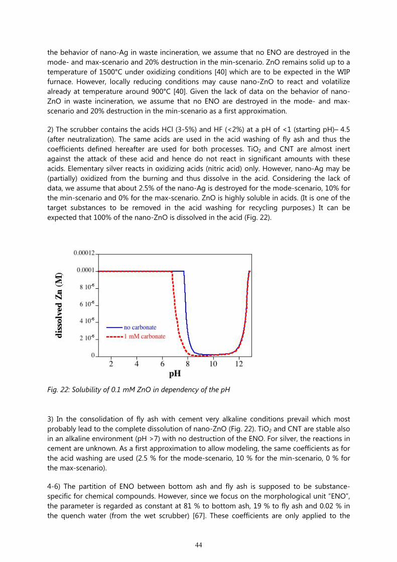
44

the behavior of nano-Ag in waste incineration, we assume that no ENO are destroyed in the mode- and max-scenario and 20% destruction in the min-scenario. ZnO remains solid up to a temperature of 1500°C under oxidizing conditions [40] which are to be expected in the WIP furnace. However, locally reducing conditions may cause nano-ZnO to react and volatilize already at temperature around 900°C [40]. Given the lack of data on the behavior of nano-ZnO in waste incineration, we assume that no ENO are destroyed in the mode- and max-scenario and 20% destruction in the min-scenario as a first approximation.

2) The scrubber contains the acids HCl (3-5%) and HF (<2%) at a pH of <1 (starting pH)– 4.5 (after neutralization). The same acids are used in the acid washing of fly ash and thus the coefficients defined hereafter are used for both processes. TiO2 and CNT are almost inert against the attack of these acid and hence do not react in significant amounts with these acids. Elementary silver reacts in oxidizing acids (nitric acid) only. However, nano-Ag may be (partially) oxidized from the burning and thus dissolve in the acid. Considering the lack of data, we assume that about 2.5% of the nano-Ag is destroyed for the mode-scenario, 10% for the min-scenario and 0% for the max-scenario. ZnO is highly soluble in acids. (It is one of the target substances to be removed in the acid washing for recycling purposes.) It can be expected that 100% of the nano-ZnO is dissolved in the acid (Fig. 22).

 

 

Fig. 22: Solubility of 0.1 mM ZnO in dependency of the pH

 

3) In the consolidation of fly ash with cement very alkaline conditions prevail which most probably lead to the complete dissolution of nano-ZnO (Fig. 22). TiO2 and CNT are stable also in an alkaline environment (pH >7) with no destruction of the ENO. For silver, the reactions in cement are unknown. As a first approximation to allow modeling, the same coefficients as for the acid washing are used (2.5 % for the mode-scenario, 10 % for the min-scenario, 0 % for the max-scenario).

4-6) The partition of ENO between bottom ash and fly ash is supposed to be substance-specific for chemical compounds. However, since we focus on the morphological unit “ENO”, the parameter is regarded as constant at 81 % to bottom ash, 19 % to fly ash and 0.02 % in the quench water (from the wet scrubber) [67]. These coefficients are only applied to the

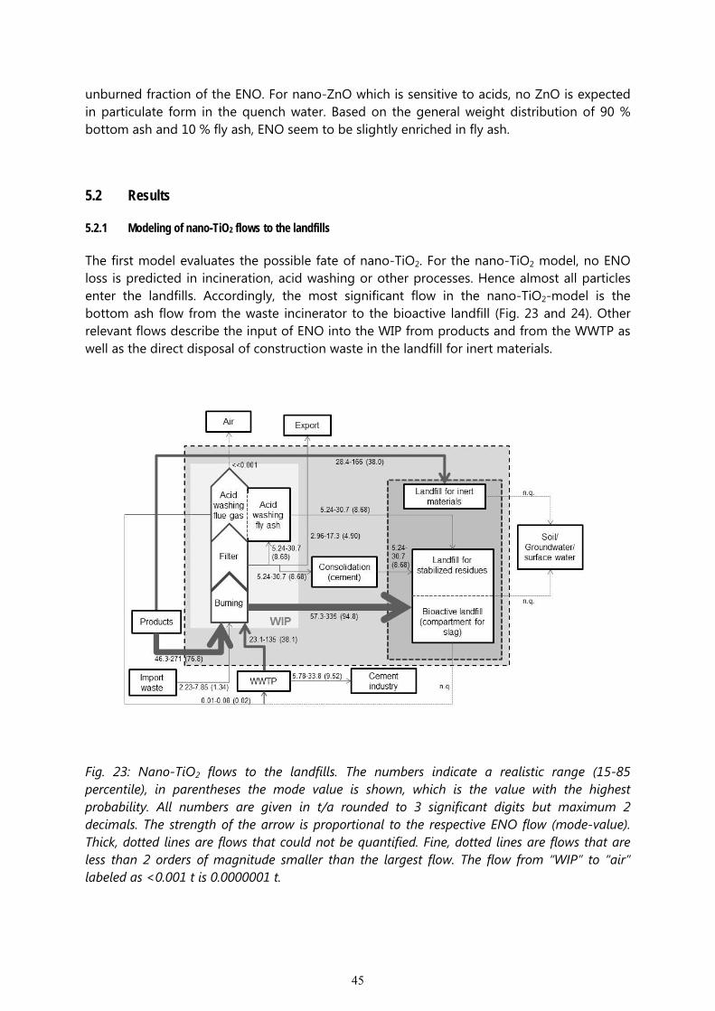
45

unburned fraction of the ENO. For nano-ZnO which is sensitive to acids, no ZnO is expected in particulate form in the quench water. Based on the general weight distribution of 90 % bottom ash and 10 % fly ash, ENO seem to be slightly enriched in fly ash.

5.2 Results

5.2.1 Modeling of nano-TiO2 flows to the landfills

The first model evaluates the possible fate of nano-TiO2. For the nano-TiO2 model, no ENO loss is predicted in incineration, acid washing or other processes. Hence almost all particles enter the landfills. Accordingly, the most significant flow in the nano-TiO2-model is the bottom ash flow from the waste incinerator to the bioactive landfill (Fig. 23 and 24). Other relevant flows describe the input of ENO into the WIP from products and from the WWTP as well as the direct disposal of construction waste in the landfill for inert materials.

 

Fig. 23: Nano-TiO2 flows to the landfills. The numbers indicate a realistic range (15-85 percentile), in parentheses the mode value is shown, which is the value with the highest probability. All numbers are given in t/a rounded to 3 significant digits but maximum 2 decimals. The strength of the arrow is proportional to the respective ENO flow (mode-value). Thick, dotted lines are flows that could not be quantified. Fine, dotted lines are flows that are less than 2 orders of magnitude smaller than the largest flow. The flow from “WIP” to “air” labeled as <0.001 t is 0.0000001 t.

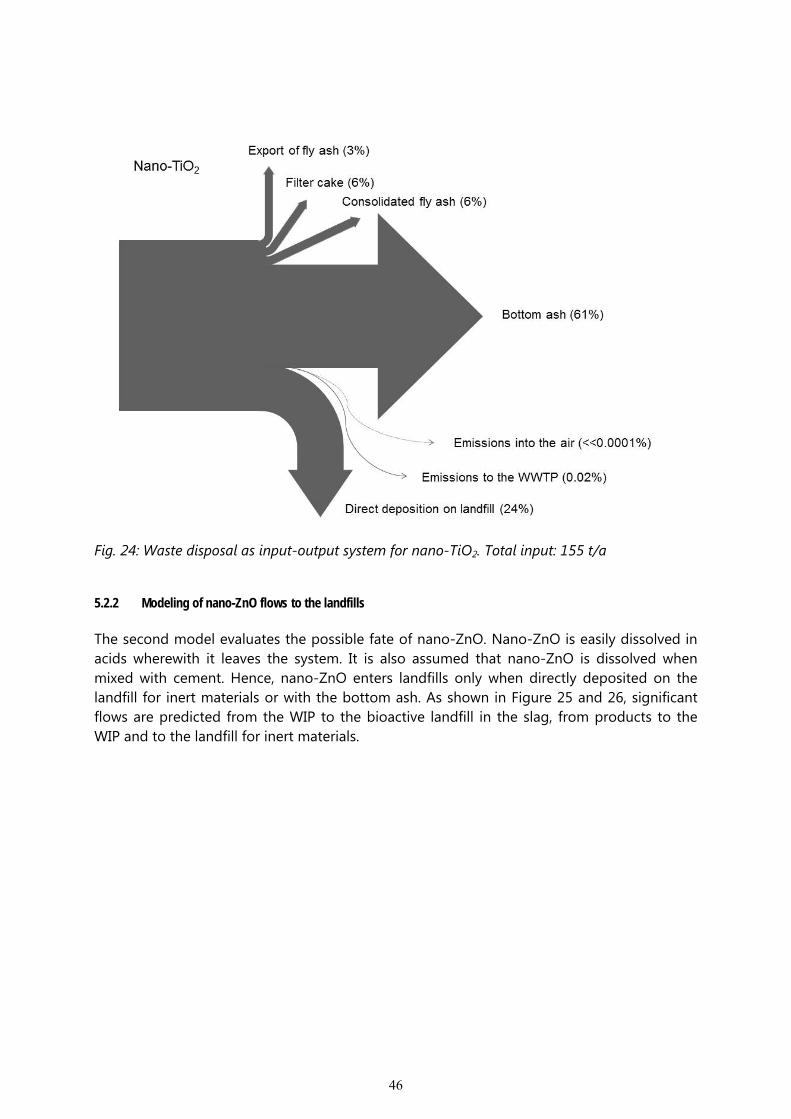
46

Fig. 24: Waste disposal as input-output system for nano-TiO2. Total input: 155 t/a

5.2.2 Modeling of nano-ZnO flows to the landfills

The second model evaluates the possible fate of nano-ZnO. Nano-ZnO is easily dissolved in acids wherewith it leaves the system. It is also assumed that nano-ZnO is dissolved when mixed with cement. Hence, nano-ZnO enters landfills only when directly deposited on the landfill for inert materials or with the bottom ash. As shown in Figure 25 and 26, significant flows are predicted from the WIP to the bioactive landfill in the slag, from products to the WIP and to the landfill for inert materials.

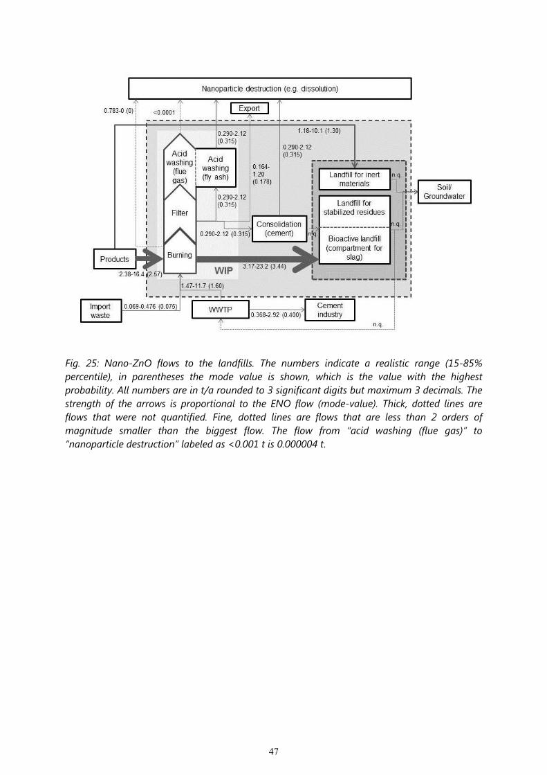
47

Fig. 25: Nano-ZnO flows to the landfills. The numbers indicate a realistic range (15-85% percentile), in parentheses the mode value is shown, which is the value with the highest probability. All numbers are in t/a rounded to 3 significant digits but maximum 3 decimals. The strength of the arrows is proportional to the ENO flow (mode-value). Thick, dotted lines are flows that were not quantified. Fine, dotted lines are flows that are less than 2 orders of magnitude smaller than the biggest flow. The flow from “acid washing (flue gas)” to “nanoparticle destruction” labeled as <0.001 t is 0.000004 t.

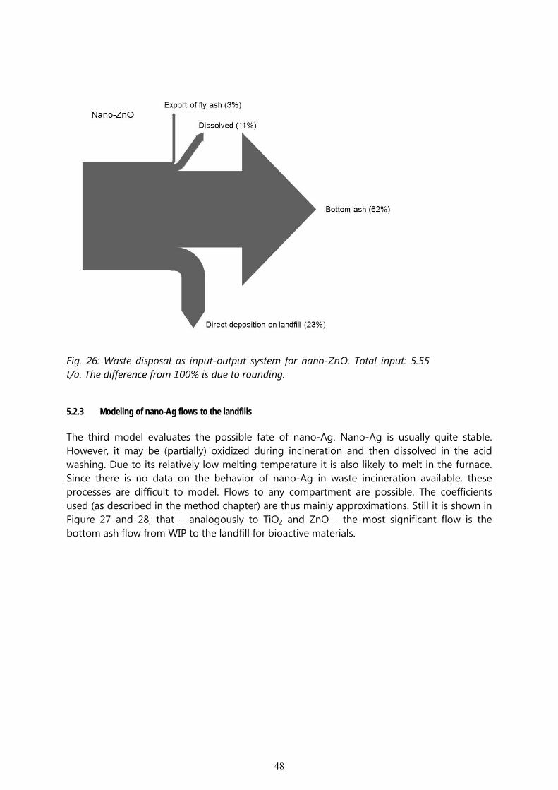
48

Fig. 26: Waste disposal as input-output system for nano-ZnO. Total input: 5.55 t/a. The difference from 100% is due to rounding.

5.2.3 Modeling of nano-Ag flows to the landfills

The third model evaluates the possible fate of nano-Ag. Nano-Ag is usually quite stable. However, it may be (partially) oxidized during incineration and then dissolved in the acid washing. Due to its relatively low melting temperature it is also likely to melt in the furnace. Since there is no data on the behavior of nano-Ag in waste incineration available, these processes are difficult to model. Flows to any compartment are possible. The coefficients used (as described in the method chapter) are thus mainly approximations. Still it is shown in Figure 27 and 28, that – analogously to TiO2 and ZnO - the most significant flow is the bottom ash flow from WIP to the landfill for bioactive materials.

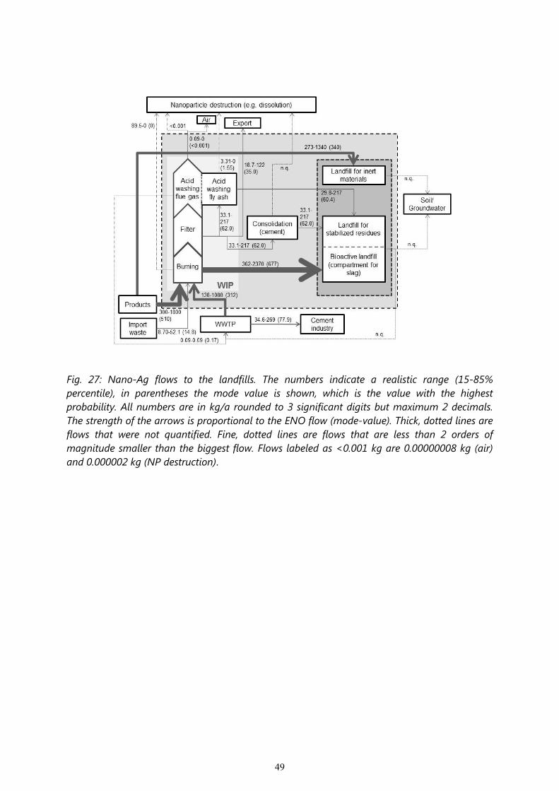
49

Fig. 27: Nano-Ag flows to the landfills. The numbers indicate a realistic range (15-85% percentile), in parentheses the mode value is shown, which is the value with the highest probability. All numbers are in kg/a rounded to 3 significant digits but maximum 2 decimals. The strength of the arrows is proportional to the ENO flow (mode-value). Thick, dotted lines are flows that were not quantified. Fine, dotted lines are flows that are less than 2 orders of magnitude smaller than the biggest flow. Flows labeled as <0.001 kg are 0.00000008 kg (air) and 0.000002 kg (NP destruction).

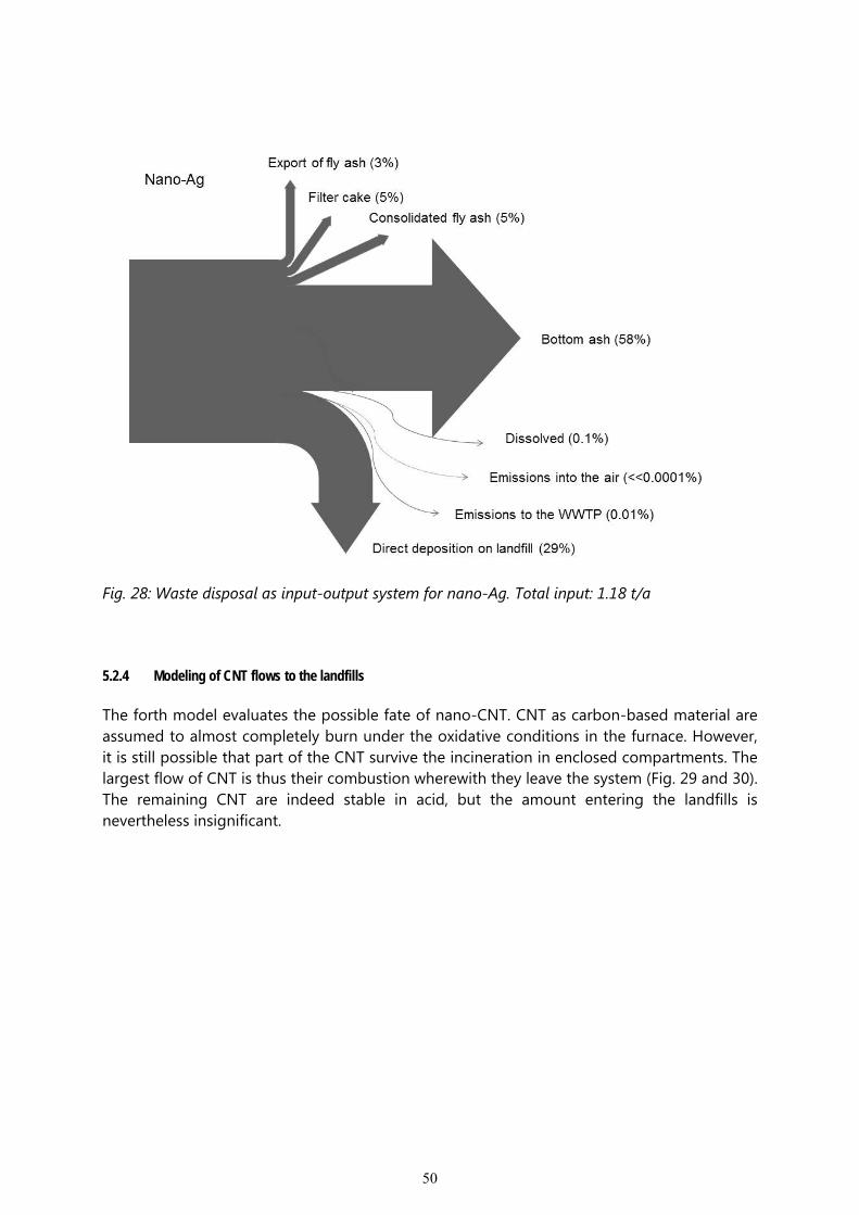
50

Fig. 28: Waste disposal as input-output system for nano-Ag. Total input: 1.18 t/a

5.2.4 Modeling of CNT flows to the landfills

The forth model evaluates the possible fate of nano-CNT. CNT as carbon-based material are assumed to almost completely burn under the oxidative conditions in the furnace. However, it is still possible that part of the CNT survive the incineration in enclosed compartments. The largest flow of CNT is thus their combustion wherewith they leave the system (Fig. 29 and 30). The remaining CNT are indeed stable in acid, but the amount entering the landfills is nevertheless insignificant.

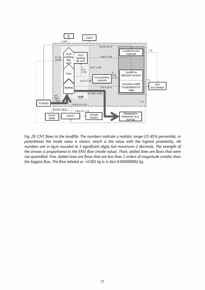
51

Fig. 29: CNT flows to the landfills. The numbers indicate a realistic range (15-85% percentile), in parentheses the mode value is shown, which is the value with the highest probability. All numbers are in kg/a rounded to 3 significant digits but maximum 2 decimals. The strength of the arrows is proportional to the ENO flow (mode-value). Thick, dotted lines are flows that were not quantified. Fine, dotted lines are flows that are less than 2 orders of magnitude smaller than the biggest flow. The flow labeled as <0.001 kg is in fact 0.000000002 kg.

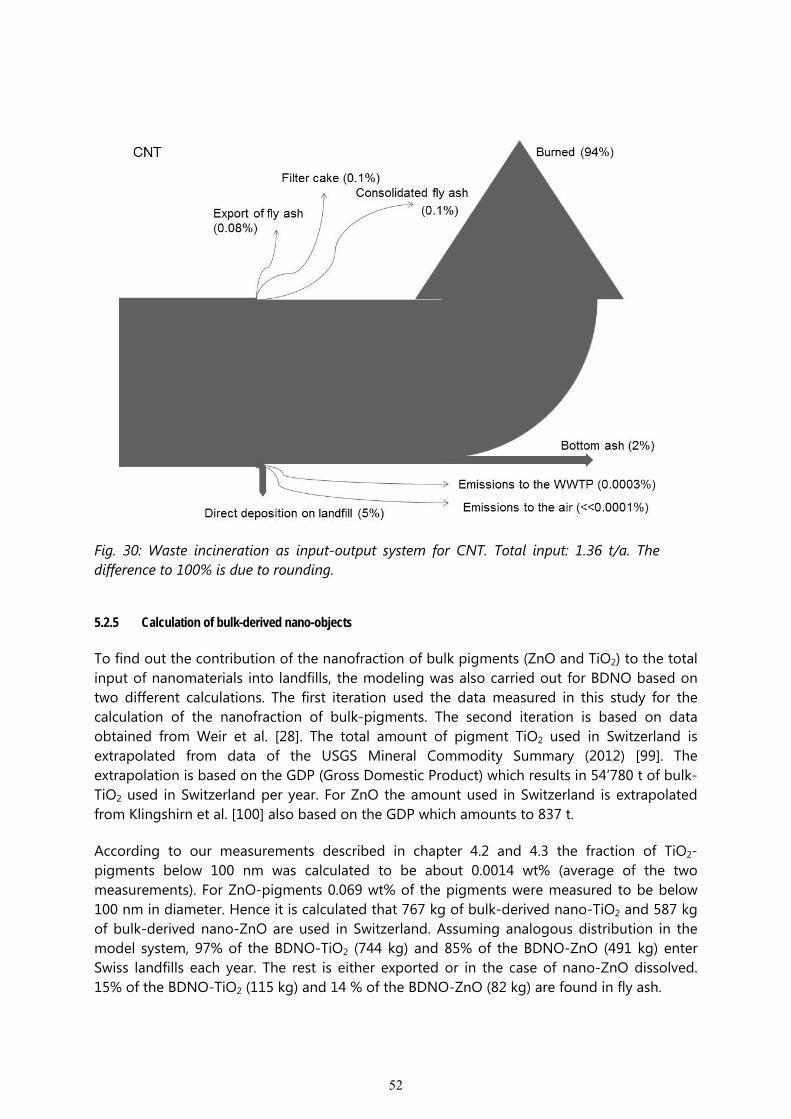
52

Fig. 30: Waste incineration as input-output system for CNT. Total input: 1.36 t/a. The difference to 100% is due to rounding.

5.2.5 Calculation of bulk-derived nano-objects

To find out the contribution of the nanofraction of bulk pigments (ZnO and TiO2) to the total input of nanomaterials into landfills, the modeling was also carried out for BDNO based on two different calculations. The first iteration used the data measured in this study for the calculation of the nanofraction of bulk-pigments. The second iteration is based on data obtained from Weir et al. [28]. The total amount of pigment TiO2 used in Switzerland is extrapolated from data of the USGS Mineral Commodity Summary (2012) [99]. The extrapolation is based on the GDP (Gross Domestic Product) which results in 54’780 t of bulk-TiO2 used in Switzerland per year. For ZnO the amount used in Switzerland is extrapolated from Klingshirn et al. [100] also based on the GDP which amounts to 837 t.

According to our measurements described in chapter 4.2 and 4.3 the fraction of TiO2-pigments below 100 nm was calculated to be about 0.0014 wt% (average of the two measurements). For ZnO-pigments 0.069 wt% of the pigments were measured to be below 100 nm in diameter. Hence it is calculated that 767 kg of bulk-derived nano-TiO2 and 587 kg of bulk-derived nano-ZnO are used in Switzerland. Assuming analogous distribution in the model system, 97% of the BDNO-TiO2 (744 kg) and 85% of the BDNO-ZnO (491 kg) enter Swiss landfills each year. The rest is either exported or in the case of nano-ZnO dissolved. 15% of the BDNO-TiO2 (115 kg) and 14 % of the BDNO-ZnO (82 kg) are found in fly ash.

53

If we take the data from Weir et al. [28], 36% (number) or 11% (weight) of conventional food-grade TiO2 is nanosized (<100 nm, measured by microscopy). Based on this value 6026 t of TiO2 used in Switzerland would be nanosized of which 97% (5845 t) end up in landfills every year. 15 % are found in fly ash (904 t).

54

6 Discussion

6.1 Measurements

ENO in products are applied in different agglomeration states. In some products ENO are intentionally kept separated, such as in commercial colloidal suspensions of nano-sized silver, gold, polystyrene latex (PSL), silica particles, etc. When these particles form agglomerates and sediment, the products lose its function. In some products (fumed silica, carbon black, TiO2) the agglomerates and aggregates of nanoparticles are formed in the production processes, e.g. flame synthesis or plasma synthesis [101, 102]. Non-agglomerated TiO2 particles are desired for pigments or composites [103] while agglomerated ones are preferred when making catalyst pellets to facilitate reactant/product flow [104, 105]. CNT often form large agglomerates of the order of microns when provided by manufacturers in powder form [106]. Such large agglomerates have limited mobility, and are easier and safer to handle and transport [107]. Because of their geometry and hydrophobic surface, CNT have a tendency to form agglomerates with a bundle-like form in aqueous media [108]. In addition to products which make use of free ENO, more and more products emerge in the composite form, i.e. ENO are embedded in certain matrices, e.g. polymer-based materials. Nanocomposites have become widely used in the industry, e.g., for sport products, paints, and coatings [109].

The agglomeration state of ENO in a product directly impacts the measurement results, thus affects categorization of the product as a nanomaterial. The results in the present study and Weir et al. [28] demonstrate that the sizes of the primary particles and agglomerates may differ substantially. The results of size distribution measurements will thus depend on how much energy was used to disperse the sample. Different dispersers for powders (brush feeder, fluidized bed, vortex shaker) and for suspensions (ultrasonicator, atomizer, spray) can be used [107]. They may break the agglomerates to a certain degree and hence change the results. The question persists even for measurement using microscopy. Is the primary particles size or the size of the agglomerates used as characteristic size of the product? ENO-producing companies will characterize their product depending on what is politically and economically advantageous. However, the EU-definition is clearly based on the primary particle size [69].

We are of the opinion that measurements should be made in the context of usage, treatment, handling, recycling and disposal of a product. The measurement should provide the most relevant sizes of the ENO. For example, if the agglomerate size is important for the function of catalyst pellets [103] then the measurement should be targeting the agglomerates. The energy used in the disperser should be comparable to what encountered by the product in its life. Schlagenhauf et al. [109] demonstrated the release of free-standing CNT from epoxy-based composite during abrasion operation. Kuhlbusch et al. [110] reviewed a number of nanoparticle emission studies in workplace for composite and coatings. On their way to a landfill, ENO may have gone through procedures such as normal usage (wear and tear, degradation), mechanical treatment, incineration, etc. It is thus difficult to predict the agglomeration state of ENO at the landfill.

Significant parts of the scientific literature on nanomaterials (e.g. nanotoxicology) work with mass units and not with particle counts. Particle size distributions based on mass will almost

55

always show a low share of particles below 100 nm based on the simple geometric relationship: one single particle with a diameter of 10 µm (with a volume of 524 μm3) has the same mass and volume as 1000 particles of 1 µm diameter from the same material. Moreover, it takes 1 billion 10 nm diameter particles to achieve an equal mass of only one 10 μm particle. As discussed in emission control also for the evaluation of the fate of ENO, a number based evaluation would be preferable.

Aerosol particles vary in size from a few nanometers to several micrometers. There is no instrument currently available to cover such a wide size range; instead a combination of several instruments is usually used. Because of the differences in the measurements principles between the instruments, difficulties arise in attempts to acquire a single size spectrum from the data measured.

It was found that the mass% below 2 µm varies significantly among the different samples. In the sample from the small scale wood-sludge incineration (WoS) the share of small particles (<2 µm) was less than 1% while in the wood incineration sample (Wo) the portion of small particles (<2 µm) was almost one third and thus even slightly larger than in the other samples. This difference might be due to the different filter type used in the WoS plant. Waste incineration plants generally use ESP while the WoS plant has a baghouse filter (fabric filter) installed. One hypothesis could be that in WoS smaller particles pass the filter. However, since all incineration plants have to meet the regulations for exhaust air, this hypothesis is not likely. Another hypothesis is that the incineration conditions in the furnace vary or the input material favours the formation of larger particles. The most probable hypothesis is that the filter type used influences the particle size distribution in the fly ash. Baghouse filters lead to the formation of a filter cake at the fabric which leads to an increased pressure at the fabric. This pressure favours particle aggregation. Hence, the particles caught in the filter cake (cleaned by back pulse) are more likely to be in an aggregated status.

In the Results part, a comparison of the samples WaS1, WaS2 and WaSA is presented. The number concentration curve of WaSA shows a bimodal size distribution and with the peaks at 270 nm and 1 µm. This sample represents an acid treated mixture of WaS1 and WaS2. The size distribution is similar to WaS1 and WaS2.

It is important to note that the particle sizes reported in our study are agglomerate sizes and not the sizes of the primary particles. The method for dispersing the particles before analysis breaks only up loose agglomerates but not aggregates. Only electron microscopic analysis of the ash together with image analysis can give information on the primary particle sizes.

6.2 Modeling

6.2.1 Limitations of the model

The model presented in chapter 5 describes a generic system of waste incineration and deposition in Switzerland. However, waste disposal in Switzerland lies within the responsibility of the cantonal (state) authorities which leads to a different management and handling of certain waste streams depending on the location of the WIP and the landfills. For example, the filter cake from acid washing of the fly ash is in some cantons mixed with the

56

bottom ash and deposited in the landfill for stabilized residues. In other cantons a separate deposition of the filter cake is required. It is also allowed to re-incinerate the filter cake from acid washing. The model is thus a simplification of the different processes evaluating a synthesis of different practices which may in reality differ from the generic model. Besides the cantonal differences in the implementation of the legislation, the 29 WIP in Switzerland also differ in their equipment (internal or external wastewater treatment, filter types, acid washing of fly ash, dry discharge of bottom ash), size and type of waste. Significant differences such as the acid washing of the filter ash, which is state of the art in about one third of the WIP in Switzerland, are reflected in the transfer coefficients used in the model.

The model combines WIP and sludge incineration. At the time there are WIP that burn exclusively waste, WIP that incinerate also sewage sludge, mono-incinerators that burn exclusively sewage sludge (SIP) and mixed systems (usually small scale) where sludge is burned together with other highly carbonaceous materials such as used wood or residues from the paper industry. While WIP produce a very heterogeneous slag, the only residue from SIP is fly ash, that has a relatively high phosphorus content. This fly ash is in some landfills deposited in a separate compartment to allow for phosphorus recovery once a cost-effective technique is available. To foster the P-recycling from sewage sludge fly ash, Switzerland aims at a strict separation of waste and sludge incineration for the year 2030. It is also discussed to distinguish five instead of three types of landfills in the near future (excavation material, inert materials (e.g. from construction), landfill for bottom ash and landfill for reactive waste). The revised legislation is planned to become effective this year.

The input data are mainly based on the study by Gottschalk et al. [22] which did not take into account any dissolution of nano-Ag and ZnO during wastewater treatment. It can thus be expected that the flows from WWTP to the WIP are smaller than indicated in the model. It has also been shown that the major Ag-form in sludge is nanoparticulate Ag2S which is formed during wastewater treatment both from dissolved Ag as well as from nano-Ag [13, 111]. The metallic nano-Ag which is used in products is therefore already transformed into another phase before it reaches the WIP. This phase is no longer separable from the mineral phase formed when dissolved Ag enters the WWTP. The further fate of Ag2S during incineration (e.g. oxidation, volatilization) is unknown.

While most of the model-specific parameters could be taken from literature or statistical data, there were no substance-specific coefficients on ENO reported in literature. Up to date, it is not known to what extend ENO are affected by waste incineration and acid washing. Extrapolations had to be made based on the physico-chemical characteristics of the respective bulk-material. Generally, it can be distinguished between combustible materials, soluble substances and stable compounds. Depending on the properties, the material may oxidize or dissolve and thus leave the system boundary “ENO”. Stable materials such as TiO2 are not lost in any process and they will accumulate either in the technosphere (e.g. landfill) or in the environment (e.g. sediments).

The slags from the WIP may be further treated on the landfill site to extract metals, e.g. iron. They may be crushed and undergo other processes that may result in generation of dust and release of ENO to the atmosphere. Due to complete lack of data about these processes and the generation of nanomaterials, they were not considered in this work but need to be investigated in further studies.

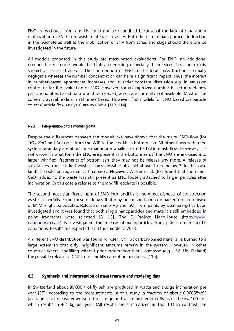
57

ENO in leachates from landfills could not be quantified because of the lack of data about mobilization of ENO from waste materials or ashes. Both the natural nanoparticulate fraction in the leachate as well as the mobilization of ENP from ashes and slags should therefore be investigated in the future.

All models proposed in this study are mass-based evaluations. For ENO, an additional number based model would be highly interesting especially if emission flows or toxicity should be assessed as well. The contribution of ENO to the total mass fraction is usually negligible whereas the number concentration can have a significant impact. Thus, the interest in number-based approaches increases and is under constant discussion e.g. in emission control or for the evaluation of ENO. However, for an improved number-based model, new particle number based data would be needed, which are currently not available. Most of the currently available data is still mass based. However, first models for ENO based on particle count (Particle flow analysis) are available [112-114].

6.2.2 Interpretation of the modeling data

Despite the differences between the models, we have shown that the major ENO-flow (for TiO2, ZnO and Ag) goes from the WIP to the landfill as bottom ash. All other flows within the system boundary are about one magnitude smaller than the bottom ash flow. However, it is not known in what form the ENO are present in the bottom ash. If the ENO are enclosed into larger (vitrified) fragments of bottom ash, they may not be release any more. A release of substances from vitrified waste is only possible at a pH above 10 or below 2. In this case landfills could be regarded as final sinks. However, Walser et al. [67] found that the nano-CeO2 added to the waste was still present as ENO loosely attached to larger particles after incineration. In this case a release to the landfill leachate is possible.

The second most significant input of ENO into landfills is the direct disposal of construction waste in landfills. From these materials that may be crushed and compacted on-site release of ENM might be possible. Release of nano-Ag and TiO2 from paints by weathering has been investigated and it was found that both single nanoparticles and materials still embedded in paint fragments were released [8, 13]. The EU-Project NanoHouse (http://www-nanohouse.cea.fr) is investigating the release of nanoparticles from paints under landfill conditions. Results are expected until the middle of 2013.

A different ENO distribution was found for CNT. CNT as carbon-based material is burned to a large extent so that only insignificant amounts remain in the system. However, in other countries where landfilling without prior incineration is still common (e.g. USA, UK, Finland) the possible release of CNT from landfills cannot be neglected [115]. 

6.3 Synthesis and interpretation of measurement and modeling data

In Switzerland about 80’000 t of fly ash are produced in waste and sludge incineration per year [97]. According to the measurements in this study, a fraction of about 0.00058wt% (average of all measurements) of the sludge and waste incineration fly ash is below 100 nm, which results in 464 kg per year. (All results are summarized in Tab. 10.) In contrast, the

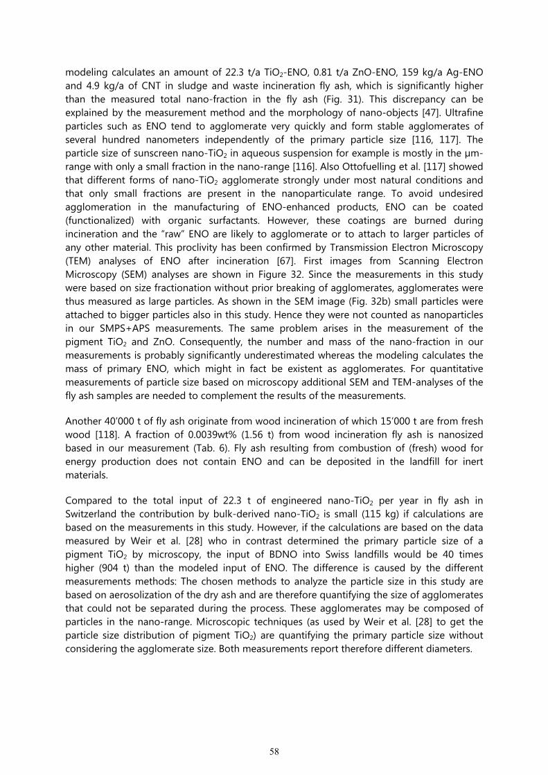
58

modeling calculates an amount of 22.3 t/a TiO2-ENO, 0.81 t/a ZnO-ENO, 159 kg/a Ag-ENO and 4.9 kg/a of CNT in sludge and waste incineration fly ash, which is significantly higher than the measured total nano-fraction in the fly ash (Fig. 31). This discrepancy can be explained by the measurement method and the morphology of nano-objects [47]. Ultrafine particles such as ENO tend to agglomerate very quickly and form stable agglomerates of several hundred nanometers independently of the primary particle size [116, 117]. The particle size of sunscreen nano-TiO2 in aqueous suspension for example is mostly in the µm-range with only a small fraction in the nano-range [116]. Also Ottofuelling et al. [117] showed that different forms of nano-TiO2 agglomerate strongly under most natural conditions and that only small fractions are present in the nanoparticulate range. To avoid undesired agglomeration in the manufacturing of ENO-enhanced products, ENO can be coated (functionalized) with organic surfactants. However, these coatings are burned during incineration and the “raw” ENO are likely to agglomerate or to attach to larger particles of any other material. This proclivity has been confirmed by Transmission Electron Microscopy (TEM) analyses of ENO after incineration [67]. First images from Scanning Electron Microscopy (SEM) analyses are shown in Figure 32. Since the measurements in this study were based on size fractionation without prior breaking of agglomerates, agglomerates were thus measured as large particles. As shown in the SEM image (Fig. 32b) small particles were attached to bigger particles also in this study. Hence they were not counted as nanoparticles in our SMPS+APS measurements. The same problem arises in the measurement of the pigment TiO2 and ZnO. Consequently, the number and mass of the nano-fraction in our measurements is probably significantly underestimated whereas the modeling calculates the mass of primary ENO, which might in fact be existent as agglomerates. For quantitative measurements of particle size based on microscopy additional SEM and TEM-analyses of the fly ash samples are needed to complement the results of the measurements.

Another 40’000 t of fly ash originate from wood incineration of which 15’000 t are from fresh wood [118]. A fraction of 0.0039wt% (1.56 t) from wood incineration fly ash is nanosized based in our measurement (Tab. 6). Fly ash resulting from combustion of (fresh) wood for energy production does not contain ENO and can be deposited in the landfill for inert materials.

Compared to the total input of 22.3 t of engineered nano-TiO2 per year in fly ash in Switzerland the contribution by bulk-derived nano-TiO2 is small (115 kg) if calculations are based on the measurements in this study. However, if the calculations are based on the data measured by Weir et al. [28] who in contrast determined the primary particle size of a pigment TiO2 by microscopy, the input of BDNO into Swiss landfills would be 40 times higher (904 t) than the modeled input of ENO. The difference is caused by the different measurements methods: The chosen methods to analyze the particle size in this study are based on aerosolization of the dry ash and are therefore quantifying the size of agglomerates that could not be separated during the process. These agglomerates may be composed of particles in the nano-range. Microscopic techniques (as used by Weir et al. [28] to get the particle size distribution of pigment TiO2) are quantifying the primary particle size without considering the agglomerate size. Both measurements report therefore different diameters.

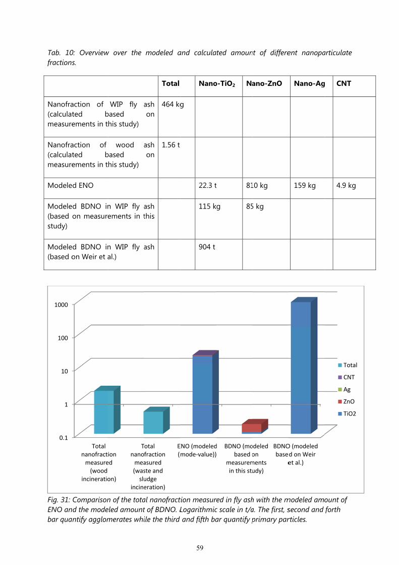
Tab. 10fractions

Nanofra(calculatmeasure

Nanofra(calculatmeasure

Modele

Modele(based study)

Modele(based o

Fig. 31: ENO anbar qua

0.1

1

10

100

1000

0: Overviews.

action of ted bements in t

action of ted bements in t

d ENO

d BDNO inon measure

d BDNO inon Weir et a

Comparisond the modentify agglom

Totalnanofractimeasure(wood

incineratio

w over the

WIP fly abased his study)

wood abased his study)

n WIP fly aements in t

n WIP fly aal.)

n of the totaeled amountmerates whi

ioned

on)

Tnanomea(wasslu

incine

modeled a

Total

ash on

464 kg

ash on

1.56 t

ash this

ash

al nanofractt of BDNO. Lile the third

otalfractionasuredste andudgeeration)

E(

59

and calcula

Nano

g

22.3 t

115 k

904 t

tion measurLogarithmicand fifth ba

ENO (modeledmode‐value))

ted amoun

o-TiO2 Na

t 81

g 85

ed in fly ashc scale in t/aar quantify p

d BDNO (mobased o

measuremin this stu

nt of differe

ano-ZnO

10 kg

5 kg

h with the ma. The first, sprimary par

odeledonmentsudy)

BDNObase

e

ent nanopa

Nano-Ag

159 kg

modeled amosecond and rticles.

O (modeledd on Weiret al.)

articulate

g CNT

4.9 kg

ount of forth

Total

CNT

Ag

ZnO

TiO2

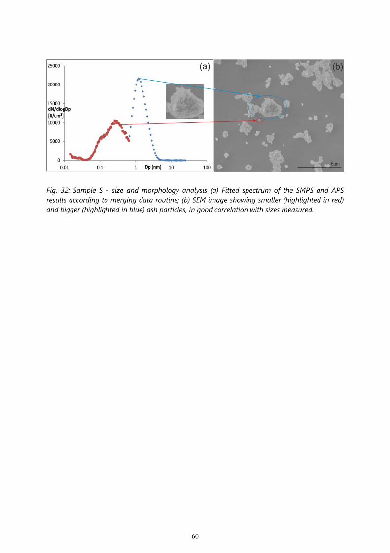
60

Fig. 32: Sample S - size and morphology analysis (a) Fitted spectrum of the SMPS and APS results according to merging data routine; (b) SEM image showing smaller (highlighted in red) and bigger (highlighted in blue) ash particles, in good correlation with sizes measured.

61

7 Outlook

The present study raises a couple of new questions which should be answered in follow-up research.

(1) It was shown that the mass-percentage of the nanosized particles in the fly ash is very small. However, the chosen measurement method is quantifying the agglomerate size and not the primary particle size. In a further study scanning and transmission electron microscopy (SEM and TEM) analyses of the fly ash samples taken are needed to get information on the primary particle size, including information on the chemical and mineralogical composition of the nano-fraction.

(2) The model used in the present study should be refined and the input parameters must be adapted to the most recent data, which will be available by 2013 (PhD thesis within NFP64 in the group of B. Nowack). A special focus has to be laid on the composition of the construction waste that is directly dumped.

(3) The measurement of the bulk-derived TiO2 and ZnO needs to be verified by TEM and SEM-analyses to take into account the primary particle size. More samples from different manufacturers and for different applications need to be investigated.

(4) Leachate from different landfills should be sampled and analyzed regarding the nanofraction and its chemical composition using state-of-the art analytical techniques, e.g. field flow fractionation coupled to ICP-MS.

(5) The dust formed during the handling of slag at the landfill site needs to be characterized in order to evaluate whether this might be an important process that leads to ENO release into the environment.

(6) The nano-fraction of the fly ash should be analyzed regarding its chemical composition and compared to the chemical composition of the fractions composed of larger particles.

(7) Lab-scale studies incinerating ENO might give information on their behavior during combustion.

(8) More samples of fly ash before and after acid washing must be taken to allow a sound interpretation of the data.

(9) The here proposed model flows were calculated using mass-based data only. However, for ENOs, an additional number based model would be interesting. The contribution of ENO to the total mass fraction is usually negligible, whereas the number concentration is more relevant for ENO. Hence, the interest in number-based approaches increases and they are also under constant discussion in emission control. However, to establish such a model, an improved data basis considering particle number based data would be needed. Nevertheless, a number-based model might largely differ to mass-based models in terms of predicted flows.

62

8 Conclusion

● The amount of ENO predicted by the mass-based models of this study to be entering Swiss landfills every year is insignificant for CNT (<100 kg/a) and very small for nano-Ag and nano-ZnO (less than a 5 t/a). However, for nano-TiO2 which is quite a widespread yet inert material, the input into Swiss landfills sums up to around 150 t/a.

● The measured fraction of nano-sized particles in the fly ash (0.00058wt%, 460 kg/a) is smaller than the modeled amount of ENO (22 t/a of nano-TiO2, 0.8 t/a nano-ZnO, 160 kg/a nano-Ag and 5 kg/a CNT).

● The discrepancy between modeled and measured data is most probably due to the measurement method which neglects the primary particles size but instead measures agglomerates.

● Microscopy analyses of the fly ash samples and further measurements e.g. in the landfill leachate are needed to validate the findings and would lead to a more conclusive assessment.

63

9 Glossary

APS Aerodynamic Particle Sizer

BDNO Bulk-derived nano-objects

CGNO Combustion-generated nano-objects

CNT Carbon Nanotubes

ENO Engineered nano-object

LS Laser scattering

Nano-Ag Nanoscale silver particles

Nano-TiO2 Nanoscale titanium dioxide particles

Nano-ZnO Nanoscale zinc oxide particles

TEM Transmission Electron Microscopy

SMPS Scanning mobility particle sizer

WIP Waste incineration plant

WWTP Waste water treatment plant

64

10 References

1. Klaine, S. J.; Koelmans, A. A.; Horne, N.; Carley, S.; Handy, R. D.; Kapustka, L.; Nowack, B.; von der Kammer, F., Paradigms to assess the environmental impact of manufactured nanomaterials. Environmental Toxicology and Chemistry 2012, 31, (1), 3-14.

2. Krystek, P.; Ulrich, A.; Garcia, C. C.; Manohar, S.; Ritsema, R., Application of plasma spectrometry for the analysis of engineered nanoparticles in suspensions and products. Journal of Analytical Atomic Spectrometry 2011, 26, (9), 1701-1721.

3. Krug, H. F.; Wick, P., Nanotoxicology: An Interdisciplinary Challenge. Angewandte Chemie-International Edition 2011, 50, (6), 1260-1278.

4. ULRICH, A.; WICHSER, A. In Analysis of additive metals in fuel and emission aerosols of diesel vehicles with and without particle traps, European Winter Conference on Plasma Spectrochemistry, SEP 2003, 2003; 2003; pp 71-81.

5. ISO, Nanotechnologies - Vocabulary. In Core terms, International Organisation for Standardisation (ISO): Geneva, 2010; Vol. ISO/TS 80004-1. 6. Som, C.; Wick, P.; Krug, H.; Nowack, B., Environmental and health effects of nanomaterials in nanotextiles and facade coatings. Environment International 2011, 37, (6), 1131-1142.

7. Geranio, L.; Heuberger, M.; Nowack, B., The Behavior of Silver Nanotextiles during Washing. Environmental Science & Technology 2009, 43, (21), 8113-8118.

8. Kaegi, R.; Ulrich, A.; Sinnet, B.; Vonbank, R.; Wichser, A.; Zuleeg, S.; Simmler, H.; Brunner, S.; Vonmont, H.; Burkhardt, M.; Boller, M., Synthetic TiO(2) nanoparticle emission from exterior facades into the aquatic environment. Environmental Pollution 2008, 156, (2), 233-239.

9. Kaegi, R.; Sinnet, B.; Zuleeg, S.; Hagendorfer, H.; Mueller, E.; Vonbank, R.; Boller, M.; Burkhardt, M., Release of silver nanoparticles from outdoor facades. Environmental Pollution 2010, 158, (9), 2900-2905.

10. Schmid, K.; Danuser, B.; Riediker, M., Nanoparticle Usage and Protection Measures in the Manufacturing Industry—A Representative Survey. Journal of Occupational and Environmental Hygiene 2010, 7, (4), 224-232. 11. Schmid, K.; Riediker, M., Use of Nanoparticles in Swiss Industry: A Targeted Survey. Environmental Science & Technology 2008, 42, (7), 2253-2260.

12. Hagendorfer, H.; Lorenz, C.; Kaegi, R.; Sinnet, B.; Gehrig, R.; Goetz, N. V.; Scheringer, M.; Ludwig, C.; Ulrich, A., Size-fractionated characterization and quantification of nanoparticle release rates from a consumer spray product containing engineered nanoparticles. Journal of Nanoparticle Research 2010, 12, (7), 2481-2494. 13. Kaegi, R.; Voegelin, A.; Sinnet, B.; Zuleeg, S.; Hagendorfer, H.; Burkhardt, M.; Siegrist, H., Behavior of Metallic Silver Nanoparticles in a Pilot Wastewater Treatment Plant. Environmental Science & Technology 2011, 45, (9), 3902-3908. 14. Ulrich, A.; Losert, S.; Bendixen, N.; Al-Kattan, A.; Hagendorfer, H.; Nowack, B.; Adlhart, C.; Ebert, J.; Lattuada, M.; Hungerbuhler, K., Critical aspects of sample handling for direct nanoparticle analysis and analytical challenges using asymmetric field flow fractionation in a multi-detector approach. Journal of Analytical Atomic Spectrometry 2012, 27, (7), 1120-1130.

15. Walser, T.; Limbach, L. K.; Brogioli, R.; Erismann, E.; Flamigni, L.; Hattendorf, B.; Juchli, M.; Krumeich, F.; Ludwig, C.; Prikopsky, K.; Rossier, M.; Saner, D.; Sigg, A.; Hellweg, S.; Gunther, D.; Stark, W. J., Persistence of engineered nanoparticles in a municipal solid-waste incineration plant. Nat Nano 2012, advance online publication.

16. Roes, L.; Patel, M. K.; Worrell, E.; Ludwig, C., Preliminary evaluation of risks related to waste incineration of polymer nanocomposites. Science of the Total Environment 2012, 417–418, 76–86.

65

17. Klaine, S. J.; Alvarez, P. J. J.; Batley, G. E.; Fernandes, T. F.; Handy, R. D.; Lyon, D. Y.; Mahendra, S.; McLaughlin, M. J.; Lead, J. R., Nanomaterials in the environment: Behavior, fate, bioavailability, and effects. Environmental Toxicology and Chemistry 2008, 27, (9), 1825-1851.

18. Menard, A.; Drobne, D.; Jemec, A., Ecotoxicity of nanosized TiO(2). Review of in vivo data. Environmental Pollution 2011, 159, (3), 677-684. 19. Ostiguy, C.; Roberge, B.; Ménard, L.; Endo, C.-A., Best Practices Guide to Synthetic Nanoparticle Risk Management; Institut de recherche Robert-Sauvé en santé et en sécurité du travail (IRSST), Commission de la santé et de la sécurité du travail du Québec (CSST) and NanoQuébec; REPORT R-599, Montréal, availabel at www.irsst.qc.ca. In 2009.

20. Mueller, N. C.; Nowack, B., Exposure Modeling of Engineered Nanoparticles in the Environment. Environmental Science & Technology 2008, 42, (12), 4447–4453. 21. Gottschalk, F.; Sonderer, T.; Scholz, R.; Nowack, B., Modeled Environmental Concentrations of Engineered Nanomaterials (TiO2, ZnO, Ag, CNT, Fullerenes) for Different Regions. Environmental Science & Technology 2009, 43, (24), 9216-9222. 22. Gottschalk, F.; Sonderer, T.; Scholz, R. W.; Nowack, B., Possibilites and limitations of modeling environmental exposure to engineered nanomaterials by probabilistic material flow analysis. Environmental Toxicology and Chemistry 2010, 29, (5), 1036-1048. 23. Hügi, M.; Gerber, P.; Hauser, A.; André Laube; Quartier, R.; Schenk, K.; Wysser, M. Abfallwirtschaftsbericht 2008. Zahlen und Entwicklungen der schweizerischen Abfallwirtschaft 2005–2007. Umwelt-Zustand Nr. 0830; Bern, 2008. 24. Hanser, C.; Kuster, J.; Gessler, R.; Ehrler, M.; Dietler, U.; Zimmermann, H.; Speck, R.; Schenk, K.; Kettler, R. EVALUATION DER ABFALLPOLITIK DES BUNDES; 2005.

25. NZZ-Folio, So viel Abfall erzeugt der Schweizer pro Jahr. NZZ Beilage 2006. 26. Bühler, A.; Schlumberger, S., Schwermetalle aus der Flugasche zurückgewinnen «Saure Flugaschewäsche – FLUWA-Verfahren» ein zukunftsweisendes Verfahren in der Abfallverbrennung, available at: http://www.bsh.ch/upload/public/0/71/BSH-Umweltservice-AG-Saure-Flugaschenwaesche-FLUWA-Verfahren.pdf. 27. Umweltbundesamt, http://www.umweltbundesamt.de/abfallwirtschaft/entsorgung/index.htm. 2012.

28. Weir, A.; Westerhoff, P.; Fabricius, L.; Hristovski, K.; von Goetz, N., Titanium Dioxide Nanoparticles in Food and Personal Care Products. Environmental Science & Technology 2012, 46, (4), 2242-2250.

29. Buseck, P. R.; Adachi, K., Nanoparticles in the Atmosphere. Elements 2008, 4, (6), 389-394. 30. Heymann, D.; Jenneskens, L. W.; Jehlicka, J.; Koper, C.; Vlietstra, E., Terrestrial and extraterrestrial fullerenes. Fullerenes Nanotubes and Carbon Nanostructures 2003, 11, (4), 333-370.

31. Murr, L. E.; Soto, K. F.; Esquivel, E. V.; Bang, J. J.; Guerrero, P. A.; Lopez, D. A.; Ramirez, D. A., Carbon nanotubes and other fullerene-related nanocrystals in the environment: A TEM study. Jom 2004, 56, (6), 28-31.

32. Giere, R.; Blackford, M.; Smith, K., TEM study of PM(2.5) emitted from coal and tire combustion in a thermal power station. Environmental Science & Technology 2006, 40, (20), 6235-6240.

33. Burtscher, H.; Zürcher, M.; Kasper, A.; Brunner, M., Efficiency of flue gas cleaning in waste incineration for submicron particles. In Proc. Int. ETH Conf. on Nanoparticle Measurement, Mayer, A., Ed. BUWAL: 2002; Vol. 52.

34. Meij, R., Trace element behavior in coal-fired power plants. Fuel Processing Technology 1994, 39, (1-3), 199-217. 35. Querol, X.; Fernandezturiel, J. L.; Lopezsoler, A., Trace elements in coal and their behavior during combustion in a large power station. Fuel 1995, 74, (3), 331-343.

66

36. Urciuolo, M.; Barone, A.; D'Alessio, A.; Chirone, R., Fine and Ultrafine Particles Generated During Fluidized Bed Combustion of Different Solid Fuels. Environmental Engineering Science 2008, 25, (10), 1399-1405.

37. Lima, A. T.; Ottosen, L. M.; Pedersen, A. J.; Ribeiro, A. B., Characterization of fly ash from bio and municipal waste. Biomass & Bioenergy 2008, 32, (3), 277-282. 38. Steenari, B. M.; Schelander, S.; Lindqvist, O., Chemical and leaching characteristics of ash from combustion of coal, peat and wood in a 12 MW CFB - a comparative study. Fuel 1999, 78, (2), 249-258.

39. Evans, J.; Williams, P. T., Heavy metal adsorption onto flyash in waste incineration flue gases. Process Safety and Environmental Protection 2000, 78, (B1), 40-46.

40. Sorum, L.; Frandsen, F. J.; Hustad, J. E., On the fate of heavy metals in municipal solid waste combustion - Part I: devolatilisation of heavy metals on the grate. Fuel 2003, 82, (18), 2273-2283. 41. Arditsoglou, A.; Petaloti, C.; Terzi, E.; Sofoniou, M.; Samara, C., Size distribution of trace elements and polycyclic aromatic hydrocarbons in fly ashes generated in Greek lignite-fired power plants. Science of the Total Environment 2004, 323, (1-3), 153-167. 42. Itskos, G.; Itskos, S.; Koukouzas, N., Size fraction characterization of highly-calcareous fly ash. Fuel Processing Technology 2010, 91, (11), 1558-1563.

43. Bhattacharjee, A.; Mandal, H.; Roy, M.; Kusz, J.; Hofmeister, W., Microstructural and magnetic characterization of fly ash from Kolaghat Thermal Power Plant in West Bengal, India. Journal of Magnetism and Magnetic Materials 2011, 323, (23), 3007-3012.

44. Noack, Y.; Sammut, M.; Depoux, M.; Ziebel, A., Comparison between baghouse-filter and electro-filter impacts on the characteristics of heavy metals emissions in a sintering plant, available at: http://www.dustconf.com/CLIENT/DUSTCONF/UPLOAD/INDUSTRI/BASIC/NOACK_F_.PDF. In.

45. Stabile, L.; Buonanno, G.; Scungio, M.; Tirler, W.; Vigo, P.; Viola, A. In Comparison of different flue gas treatment sections in the abatement of ultrafine particles emitted by waste incinerators, 15th ETH-Conference on Combustion Generated Nanoparticles, Zurich, 2011; Zurich, 2011.

46. Chang, F. Y.; Wey, M. Y., Comparison of the characteristics of bottom and fly ashes generated from various incineration processes. Journal of Hazardous Materials 2006, 138, (3), 594-603. 47. Le Forestier, L.; Libourel, G., Characterization of flue gas residues from municipal solid waste combustors. Environmental Science & Technology 1998, 32, (15), 2250-2256.

48. Thipse, S. S.; Schoenitz, M.; Dreizin, E. L., Morphology and composition of the fly ash particles produced in incineration of municipal solid waste. Fuel Processing Technology 2002, 75, (3), 173-184.

49. Pedersen, A. J.; Frandsen, F. J.; Riber, C.; Astrup, T.; Thomsen, S. N.; Lundtorp, K.; Mortensen, L. F., A Full-scale Study on the Partitioning of Trace Elements in Municipal Solid Waste Incineration-Effects of Firing Different Waste Types. Energy & Fuels 2009, 23, (7), 3475-3489.

50. Chen, C. Y.; Wang, H. P.; Wei, Y. L.; Jou, C. J. G.; Huang, Y. C., Observation of nano copper in waste heat boiler fly ashes. Radiation Physics and Chemistry 2006, 75, (11), 1913-1915. 51. Kim, W. S.; Park, M.; Lee, D. W.; Moon, M. H.; Lim, H.; Lee, S., Size-based analysis of incinerator fly ash using gravitational SPLITT fractionation, sedimentation field-flow fractionation, and inductively coupled plasma-atomic emission spectroscopy. Analytical and Bioanalytical Chemistry 2004, 378, (3), 746-752.

52. Romero, M.; Rawlings, R. D.; Rincon, J. M., Development of a new glass-ceramic by means of controlled vitrification and crystallisation of inorganic wastes from urban incineration. Journal of the European Ceramic Society 1999, 19, (12), 2049-2058.

53. Eidgenössisches Departement für Umwelt, V., Energie und Kommunikation UVEK,, Positionspapier Feinstaub aus Holzfeuerungen. In 2006. 54. Brenn, J.; Schmatloch, V. Europäische Patentanmeldung EP 1 193 445 A2 - Vorrichtung zur Rauchgasreinigung an Kleinfeuerungen. 2002.

55. Schmatloch, V. Europäische Patentanmeldung EP 1.967.273 A2 - Elektrofilter für eine Kleinfeuerungsanlage. 2008.

67

56. Luftreinhalteverordnung der Schweiz (LRV): http://www.admin.ch/ch/d/sr/8/814.318.142.1.de.pdf. In 2010. 57. Amt für Lebensmittelkontrolle und Umweltschutz, Entsorgung von Asche aus Cheminées und Holzheizungen, available at: http://www.interkantlab.ch/fileadmin/filesharing/dokumente/Merkblaetter/MerkAscheentsorgung.pdf (last visit: April 2012). In 2009.

58. Kroppl, M.; Munoz, I. L.; Zeiner, M., Trace elemental characterization of fly ash. Toxicological and Environmental Chemistry 2011, 93, (5), 886-894. 59. Osan, J.; Alfoldy, B.; Torok, S.; Van Grieken, R., Characterisation of wood combustion particles using electron probe microanalysis. Atmospheric Environment 2002, 36, (13), 2207-2214.

60. Poykio, R.; Ronkkomaki, H.; Nurmesniemi, H.; Peramaki, P.; Popov, K.; Valimaki, I.; Tuomi, T., Chemical and physical properties of cyclone fly ash from the grate-fired boiler incinerating forest residues at a small municipal district heating plant (6 MW). Journal of Hazardous Materials 2009, 162, (2-3), 1059-1064. 61. Lanzerstorfer, C., Model based prediction of required cut size diameter for fractionation of fly ash from a grate-fired wood chip incineration plant. Fuel Processing Technology 2011, 92, (5), 1095-1100. 62. Dahl, O.; Nurmesniemi, H.; Poykio, R.; Watkins, G., Comparison of the characteristics of bottom ash and fly ash from a medium-size (32 MW) municipal district heating plant incinerating forest residues and peat in a fluidized-bed boiler. Fuel Processing Technology 2009, 90, (7-8), 871-878. 63. Ronkkomaki, H.; Poykio, R.; Nurmesniemi, H.; Popov, K.; Merisalu, E.; Tuomi, T.; Valimaki, L., Particle size distribution and dissolution properties of metals in cyclone fly ash. International Journal of Environmental Science and Technology 2008, 5, (4), 485-494. 64. Asmatulu, E.; Twomey, J.; Overcash, M., Life cycle and nano-products: end-of-life assessment. Journal of Nanoparticle Research 2012, 14, (3).

65. Bystrzejewska-Piotrowska, G.; Golimowski, J.; Urban, P. L., Nanoparticles: Their potential toxicity, waste and environmental management. Waste Management 2009, 29, (9), 2587-2595. 66. Musee, N., Nanowastes and the environment: Potential new waste management paradigm. Environment International 2011, 37, (1), 112-128.

67. Walser, T.; Limbach, L. K.; Brogioli, R.; Erismann, E.; Flamigni, L.; Hattendorf, B.; Juchli, M.; Krumeich, F.; Ludwig, C.; Prikopsky, K.; Rossier, M.; Saner, D.; Sigg, A.; Hellweg, S.; Günther, D.; Stark, W. J., Persistence of engineered nanoparticles in a municipal solid-waste incineration plant. Nature Nanotechnology 2012, in press. 68. Sørum, L.; Fossum, M.; Evensen, E.; Hustad, J. In Heavy metal partitioning in a municipal solid waste incinerator, Fifth Annual North American Waste-to-Energy Conference, 1997; 1997.

69. European Commission, COMMISSION RECOMMENDATION of 18 October 2011 on the definition of nanomaterial. Official Journal of the European Union 2011.

70. Thiele, E. S.; French, R. H., Light-scattering properties of representative, morphological rutile titania particles studied using a finite-element method. Journal of the American Ceramic Society 1998, 81, (3), 469-479.

71. DuPont DuPont™ RPS Vantage®: http://www2.dupont.com/Titanium_Technologies/en_US/products/rps_vantage/PA_B_RPS_Vantage_Product_Description_H_60168_8.pdf (April 2012, last visit).

72. Gori, M.; Bergfeldt, B.; Pfrang-Stotz, G.; Reichelt, J.; Sirini, P., Effect of short-term natural weathering on MSWI and wood waste bottom ash leaching behaviour. Journal of Hazardous Materials 2011, 189, (1-2), 435-443.

73. Ludwig, C.; Johnson, C. A.; Kappeli, M.; Ulrich, A.; Riediker, S., Hydrological and geochemical factors controlling the leaching of cemented MSWI air pollution control residues: A lysimeter field study. Journal of Contaminant Hydrology 2000, 42, (2-4), 253-272

68

74. Johnson, C. A.; Kersten, M.; Ziegler, F.; Moor, H. C., Leaching behaviour and solubility — Controlling solid phases of heavy metals in municipal solid waste incinerator ash. Waste Management 1996, 16, (1-3), 129-134.

75. Johnson, C. A.; Kaeppeli, M.; Brandenberger, S.; Ulrich, A.; Baumann, W., Hydrological and geochemical factors affecting leachate composition in municipal solid waste incinerator bottom ash: Part II. The geochemistry of leachate from Landfill Lostorf, Switzerland. Journal of Contaminant Hydrology 1999, 40, (3), 239-259.

76. Zweifel, H.-R.; Johnson, C. A.; Hoehn, E., Langzeitanalysen der Hauptelemente von Sickerwässern aus Altdeponien. Fachzeitschrift für Abfall- und Ressourcenwirtschaft 1999, 12, 727 - 732.

77. Johnson, C. A.; Richner, G. A.; Vitvar, T.; Schittli, N.; Eberhard, M., Hydrological and geochemical factors affecting leachate composition in municipal solid waste incinerator bottom ash: Part I: The hydrology of Landfill Lostorf, Switzerland. Journal of Contaminant Hydrology 1998, 33, (3–4), 361-376.

78. Johnson, C. A.; Kersten, M.; Ziegler, F.; Moor, H. C., Leaching behaviour and solubility — Controlling solid phases of heavy metals in municipal solid waste incinerator ash. Waste Management 1996, 16, (1–3), 129-134.

79. Hofer, M.; Aeschbach-Hertig, W.; Beyerle, U.; Haderlein, S. B.; Hoehn, E.; Hofstetter, T. B.; Johnson, A.; Kipfer, R.; Ulrich, A.; Imboden, D. M., Tracers as essential tools for the investigation of physical and chemical processes in groundwater systems. Chimia 1997, 51, (12), 941-946.

80. Lou, Z. Y.; Dong, B.; Chai, X. L.; Song, Y.; Zhao, Y. C.; Zhu, N. W., Characterization of refuse landfill leachates of three different stages in landfill stabilization process. Journal of Environmental Sciences-China 2009, 21, (9), 1309-1314.

81. Lou, Z. Y.; Zhao, Y. C., Size-fractionation and characterization of refuse landfill leachate by sequential filtration using membranes with varied porosity. Journal of Hazardous Materials 2007, 147, (1-2), 257-264.

82. Jensen, D. L.; Christensen, T. H., Colloidal and dissolved metals in leachates from four Danish landfills. Water Research 1999, 33, (9), 2139-2147.

83. Gounaris, V.; Anderson, P. R.; Holsen, T. M., Characteristics and environmental significance of colloids in landfill leachate. Environmental Science & Technology 1993, 27, (7), 1381-1387.

84. Hügi, M.; Gerber, P.; Schenk, K.; Laube, A.; Quartier, R.; Vögeli, Y. Bericht Abfallstatistik 2004. Zahlen und Entwicklungen der schweizerischen Abfallwirtschaft im Jahr 2004. Umwelt-Zustand Nr. 0638.; Bern, 2006.

85. EU, http://europa.eu/legislation_summaries/environment/waste_management/index_de.htm.

86. Reinhart, D. R.; Berge, N. D.; Bolyard, S. C.; Santra, S., Emerging contaminants: Nanomaterial fate in landfills. Waste Management 2010, 30, 2020-2021.

87. DeCarlo, P. F.; Slowik, J. G.; Worsnop, D. R.; Davidovits, P.; Jimenez, J. L., Particle morphology and density characterization by combined mobility and aerodynamic diameter measurements. Part 1: Theory. Aerosol Science and Technology 2004, 38, (12), 1185-1205.

88. Beddows, D. C. S.; Dall'osto, M.; Harrison, R. M., An Enhanced Procedure for the Merging of Atmospheric Particle Size Distribution Data Measured Using Electrical Mobility and Time-of-Flight Analysers. Aerosol Science and Technology 2010, 44, (11), 930-938.

89. Khlystov, A.; Stanier, C.; Pandis, S. N., An Algorithm for Combining Electrical Mobility and Aerodynamic Size Distributions Data when Measuring Ambient Aerosol Special Issue of Aerosol Science and Technology on Findings from the Fine Particulate Matter Supersites Program. Aerosol Science and Technology 2004, 38, (sup1), 229-238.

90. Schmid, O.; Karg, E.; Hagen, D. E.; Whitefield, P. D.; Ferron, G. A., On the effective density of non-spherical particles as derived from combined measurements of aerodynamic and mobility equivalent size. Journal of Aerosol Science 2007, 38, (4), 431-443.

69

91. Hudson, P. K.; Gibson, E. R.; Young, M. A.; Kleiber, P. D.; Grassian, V. H., A Newly Designed and Constructed Instrument for Coupled Infrared Extinction and Size Distribution Measurements of Aerosols. Aerosol Science and Technology 2007, 41, (7), 701-710.

92. Koponen, I. K.; Jensen, K. A.; Schneider, T., Sanding dust from nanoparticle-containing paints: Physical characterisation. Journal of Physics: Conference Series 2009, 151, (1), 012048. 93. Kuo, Y.-M.; Huang, S.-H.; Shih, T.-S.; Chen, C.-C.; Weng, Y.-M.; Lin, W.-Y., Development of a Size-Selective Inlet-Simulating ICRP Lung Deposition Fraction. Aerosol Science and Technology 2005, 39, (5), 437-443. 94. Maguhn, J.; Karg, E.; Kettrup, A.; Zimmermann, R., On-line Analysis of the Size Distribution of Fine and Ultrafine Aerosol Particles in Flue and Stack Gas of a Municipal Waste Incineration Plant:  Effects of Dynamic Process Control Measures and Emission Reduction Devices. Environmental Science & Technology 2003, 37, (20), 4761-4770.

95. Seinfeld, J. H.; Pandis, S. N., Atmospheric chemistry and physics: from air pollution to climate change. Wiley: 2006. 96. Hinds, W. C., Aerosol Technology: Properties, Behavior, and Measurement of Airborne Particles 1999.

97. Frey, B. Total Revision TVA, http://kommunale-infrastruktur.ch/cmsfiles/bafu_frey.pdf; 2010. 98. Baccini, P.; Brunner, P. H., Metabolism of the Anthorposphere. Springer-Verlag: Berlin, Heidelberg, New York, 1991.

99. USGS, U.S. Geological Survey, Mineral commodity summaries 2012. 2012. 100. Klingshirn, C., ZnO: Material, physics and applications. Chemphyschem 2007, 8, (6), 782-803.

101. Wang, J.; Shin, W. G.; Mertler, M.; Sachweh, B.; Fissan, H.; Pui, D. Y. H., Measurement of Nanoparticle Agglomerates by Combined Measurement of Electrical Mobility and Unipolar Charging Properties. Aerosol Science and Technology 2010, 44, (2), 97 — 108.

102. Leparoux, M.; Schreuders, C.; Shin, J. W.; Siegmann, S., Induction Plasma Synthesis of Carbide Nano-Powders. Advanced Engineering Materials 2005, 7, (5), 349-353.

103. Mueller, R.; Kammler, H. K.; Pratsinis, S. E.; Vital, A.; Beaucage, G.; Burtscher, P., Non-agglomerated dry silica nanoparticles. Powder Technology 2004, 140, (1-2), 40-48.

104. Kammler, H. K.; Madler, L.; Pratsinis, S. E., Flame synthesis of nanoparticles. Chemical Engineering and Technology 2001, 24, (6), 583–596. 105. Teleki, A.; Wengeler, R.; Wengeler, L.; Nirschl, H.; Pratsinis, S. E., Distinguishing between aggregates and agglomerates of flame-made TiO2 by high-pressure dispersion. Powder Technology 2008, 181, 292–300. 106. Kim, S. C.; Chen, D. R.; Qi, C.; Gelein, R. M.; Finkelstein, J. N.; Elder, A.; Bentley, K.; Oberdorster, G.; Pui, D. Y. H., A nanoparticle dispersion method for in vitro and in vivo nanotoxicity study. Nanotoxicology 2010, 4, (1), 42-51. 107. Wang, J.; Pui, D. Y. H., Dispersion and filtration of carbon nanotubes (CNTs) and measurement of nanoparticle agglomerates in diesel exhaust. Chem. Eng. Sci 2012, in press.

108. Wick, P.; Manser, P.; Limbach, L. K.; Dettlaff-Weglikowska, U.; Krumeich, F.; Roth, S.; Stark, W. J.; Bruinink, A., The degree and kind of agglomeration affect carbon nanotube cytotoxicity. Toxicology Letters 2007, 168, (2), 121-131.

109. Schlagenhauf, L.; Chu, B. T. T.; Buha, J.; Nüesch, F.; Wang, J., Release of carbon nanotubes from an epoxy-based nanocomposite during an abrasion process. Environ. Sci. Technol. 2012, in press.

110. Kuhlbusch, T. A. J.; Asbach, C.; Fissan, H.; Goehler, D.; Stintz, M., Nanoparticle exposure at nanotechnology workplaces: A review. Part. Fibre Toxicol. 2011, 8, (22). 111. Kim, B.; Park, C. S.; Murayama, M.; Hochella, M. F., Discovery and Characterization of Silver Sulfide Nanoparticles in Final Sewage Sludge Products. Environmental Science & Technology 2010, 44, (19), 7509-7514.

70

112. Arvidsson, R.; Molander, S.; Sanden, B. A., Impacts of a Silver-Coated Future. Journal of Industrial Ecology 2011, 15, (6), 844-854. 113. Arvidsson, R.; Molander, S.; Sanden, B. A.; Hassellov, M., Challenges in Exposure Modeling of Nanoparticles in Aquatic Environments. Human and Ecological Risk Assessment 2011, 17, (1), 245-262.

114. Arvidsson, R.; Molander, S.; Sanden, B. A., Particle Flow Analysis. Journal of Industrial Ecology 2012, 16, (3).

115. Nowack, B.; Brouwer, D.; Fissan, H.; Dahm, M.; Morris, H.; Voetz, M.; Thomas, T.; Zepp, R.; David, R.; Isaacs, J.; Libelo, L.; Shatkin, J. A.; Miller, M. B.; Stintz, M.; Sandy, M. Task Group 3 White Paper Draft: Potential Release Scenarios for Multi-Walled Carbon Nanotubes (MWCNT) from Composites; 2012.

116. Labille, J.; Feng, J. H.; Botta, C.; Borschneck, D.; Sammut, M.; Cabie, M.; Auffan, M.; Rose, J.; Bottero, J. Y., Aging of TiO2 nanocomposites used in sunscreen. Dispersion and fate of the degradation products in aqueous environment. Environmental Pollution 2010, 158, (12), 3482-3489.

117. Ottofuelling, S.; Von der Kammer, F.; Hofmann, T., Commercial Titanium Dioxide Nanoparticles in Both Natural and Synthetic Water: Comprehensive Multidimensional Testing and Prediction of Aggregation Behavior. Environmental Science & Technology 2011, 45, (23), 10045-10052.

118. Augustin, S.; Bernasconi, A.; Suter, C.-L. Holzasche und Wald - Auslegeordnung und Bericht zum BAFU-Workshop vom 24. März 2010; 2012.