VECTOR CALCULUSVECTOR CALCULUS

16

16.4Green’s Theorem

In this section, we will learn about:

Green’s Theorem for various regions and

its application in evaluating a line integral.

VECTOR CALCULUS

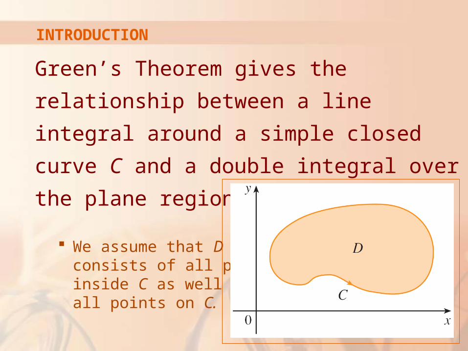
INTRODUCTION

Green’s Theorem gives the relationship

between a line integral around a simple closed

curve C and a double integral over the plane

region D bounded by C.

We assume that D consists of all points inside C as well as all points on C.

INTRODUCTION

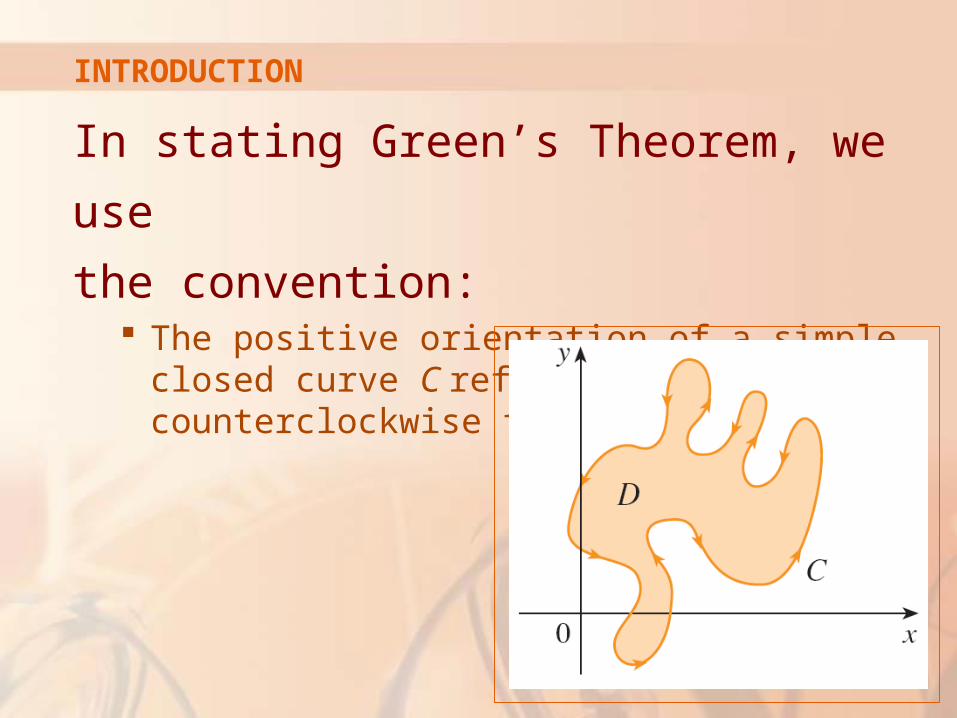
In stating Green’s Theorem, we use

the convention: The positive orientation of a simple closed curve C

refers to a single counterclockwise traversal of C.

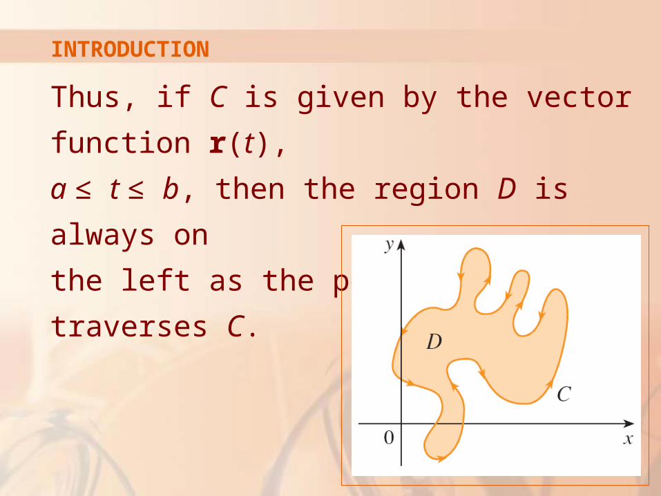
INTRODUCTION

Thus, if C is given by the vector function r(t),

a ≤ t ≤ b, then the region D is always on

the left as the point r(t) traverses C.

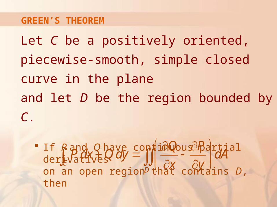
GREEN’S THEOREM

Let C be a positively oriented, piecewise-

smooth, simple closed curve in the plane

and let D be the region bounded by C.

If P and Q have continuous partial derivatives on an open region that contains D, then

CD

Q PP dx Q dy dA

x y

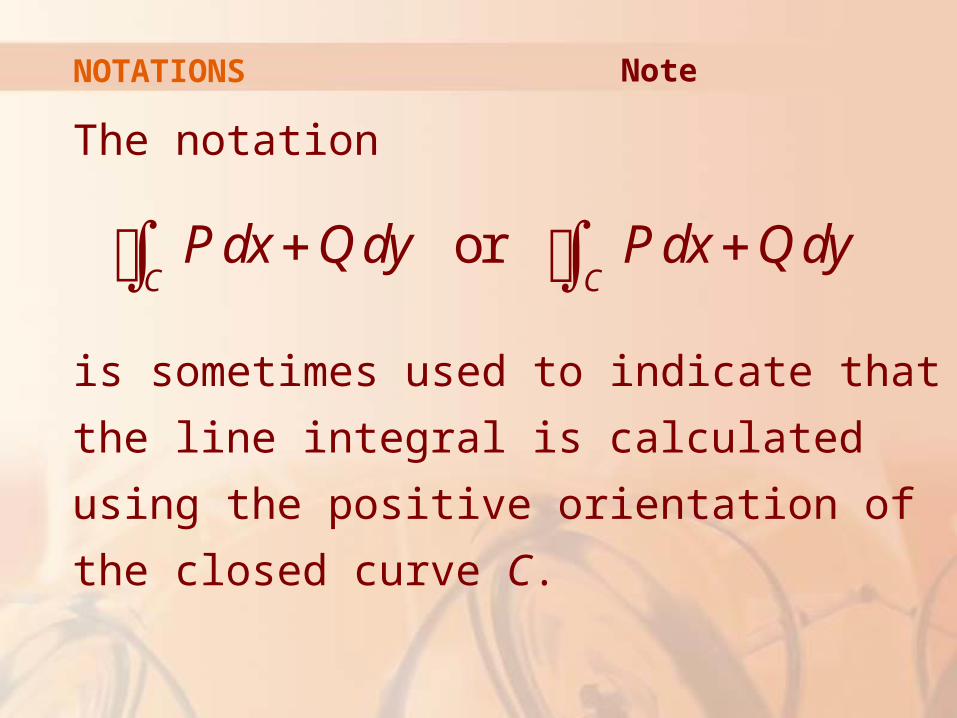
NOTATIONS

The notation

is sometimes used to indicate that the line

integral is calculated using the positive

orientation of the closed curve C.

Note

or C CP dx Q dy P dx Q dy

NOTATIONS

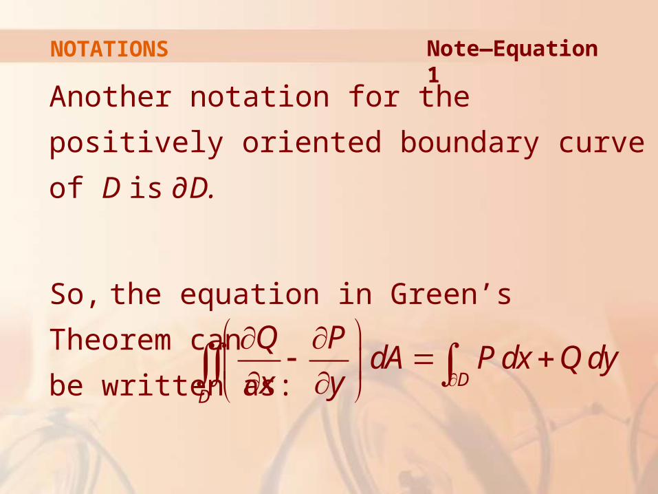
Another notation for the positively oriented

boundary curve of D is ∂D.

So, the equation in Green’s Theorem can

be written as:

DD

Q PdA P dx Q dy

x y

Note—Equation 1

GREEN’S THEOREM

Green’s Theorem should be regarded

as the counterpart of the Fundamental

Theorem of Calculus (FTC) for double

integrals.

GREEN’S THEOREM

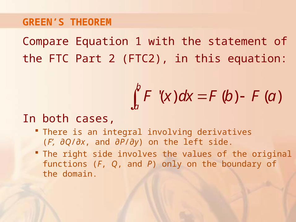
Compare Equation 1 with the statement of

the FTC Part 2 (FTC2), in this equation:

In both cases, There is an integral involving derivatives

(F’, ∂Q/∂x, and ∂P/∂y) on the left side. The right side involves the values of the original

functions (F, Q, and P) only on the boundary of the domain.

'( ) ( ) ( )b

aF x dx F b F a

GREEN’S THEOREM

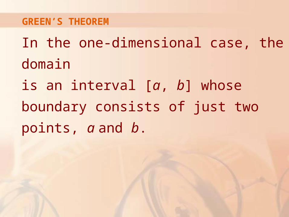
In the one-dimensional case, the domain

is an interval [a, b] whose boundary

consists of just two points, a and b.

SIMPLE REGION

The theorem is not easy to prove in general.

Still, we can give a proof for the special case

where the region is both of type I and type II

(Section 15.3).

Let’s call such regions simple regions.

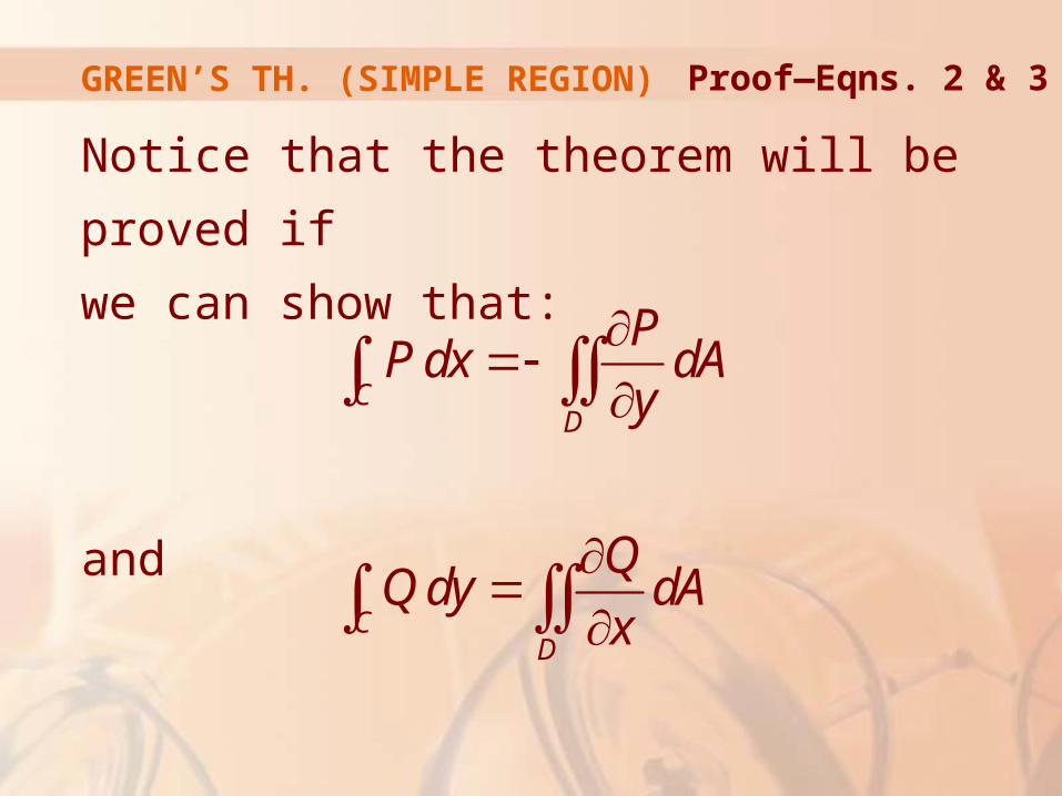
GREEN’S TH. (SIMPLE REGION)

Notice that the theorem will be proved if

we can show that:

and

Proof—Eqns. 2 & 3

CD

CD

PP dx dA

y

QQ dy dA

x

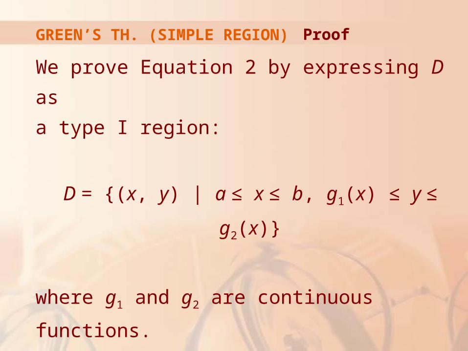
GREEN’S TH. (SIMPLE REGION)

We prove Equation 2 by expressing D as

a type I region:

D = {(x, y) | a ≤ x ≤ b, g1(x) ≤ y ≤ g2(x)}

where g1 and g2 are continuous functions.

Proof

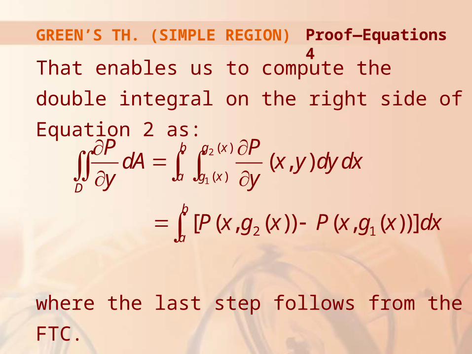
GREEN’S TH. (SIMPLE REGION)

That enables us to compute the double

integral on the right side of Equation 2 as:

where the last step follows from the FTC.

Proof—Equations 4

2

1

( )

( )

2 1

( , )

[ ( , ( )) ( , ( ))]

b g x

a g xD

b

a

P PdA x y dy dx

y y

P x g x P x g x dx

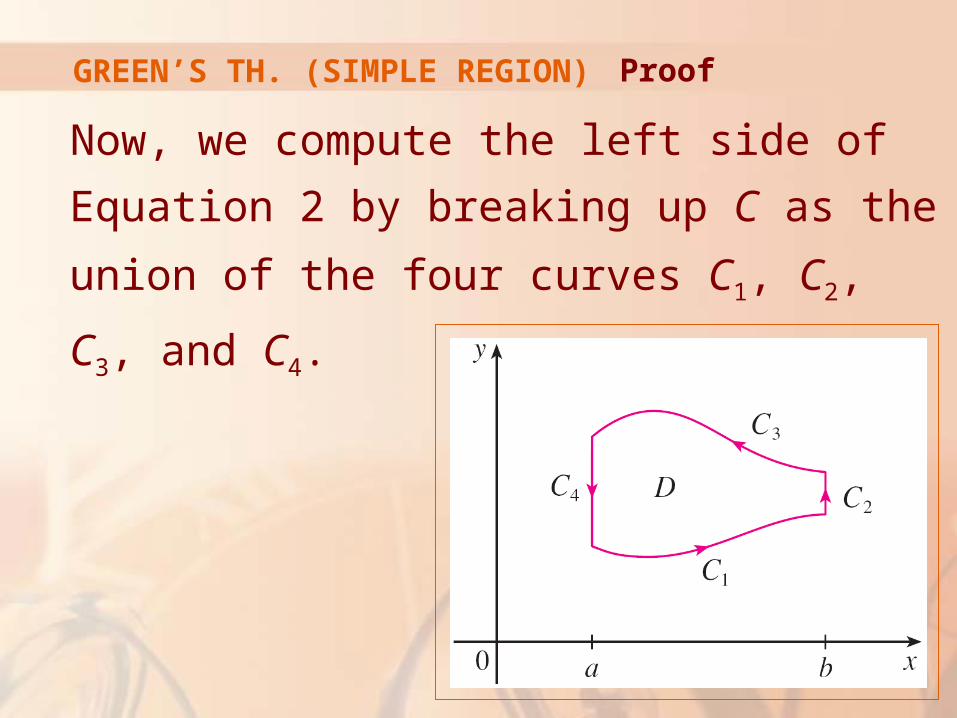
GREEN’S TH. (SIMPLE REGION)

Now, we compute the left side of Equation 2

by breaking up C as the union of the four

curves C1, C2, C3, and C4.

Proof

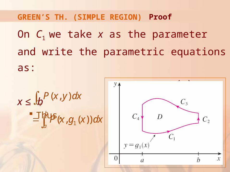
GREEN’S TH. (SIMPLE REGION)

On C1 we take x as the parameter and write

the parametric equations as:

x = x, y = g1(x), a ≤ x ≤ b Thus,

Proof

1

1

( , )

( , ( ))

C

b

a

P x y dx

P x g x dx

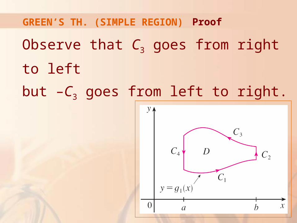
GREEN’S TH. (SIMPLE REGION)

Observe that C3 goes from right to left

but –C3 goes from left to right.

Proof

GREEN’S TH. (SIMPLE REGION)

So, we can write the parametric equations

of –C3 as: x = x, y = g2(x), a ≤ x ≤ b

Therefore,

3

3

2

( , )

( , )

( , ( ))

C

C

b

a

P x y dx

P x y dx

P x g x dx

Proof

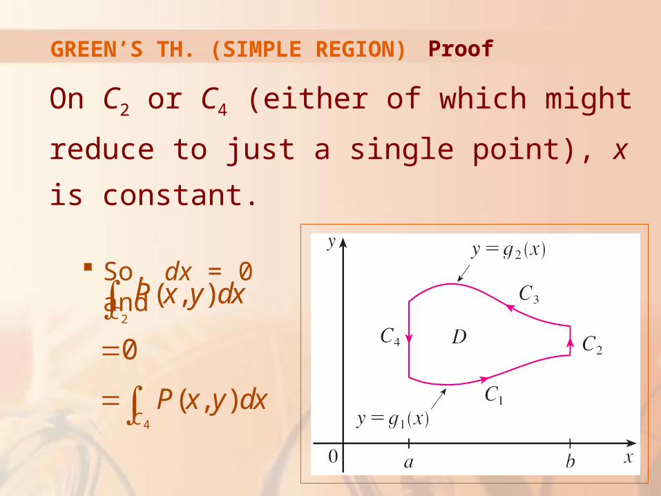
GREEN’S TH. (SIMPLE REGION)

On C2 or C4 (either of which might reduce to

just a single point), x is constant.

So, dx = 0 and

2

4

( , )

0

( , )

C

C

P x y dx

P x y dx

Proof

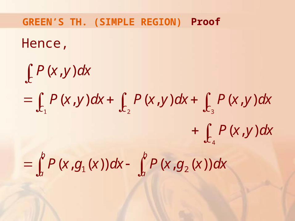
GREEN’S TH. (SIMPLE REGION)

Hence,

1 2 3

4

1 2

( , )

( , ) ( , ) ( , )

( , )

( , ( )) ( , ( ))

C

C C C

C

b b

a a

P x y dx

P x y dx P x y dx P x y dx

P x y dx

P x g x dx P x g x dx

Proof

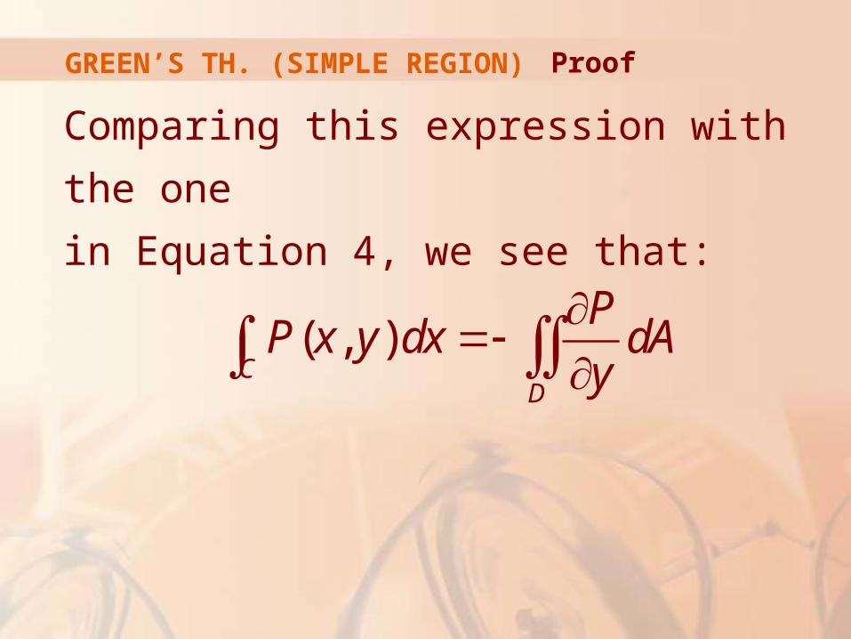
GREEN’S TH. (SIMPLE REGION)

Comparing this expression with the one

in Equation 4, we see that:

Proof

( , )C

D

PP x y dx dA

y

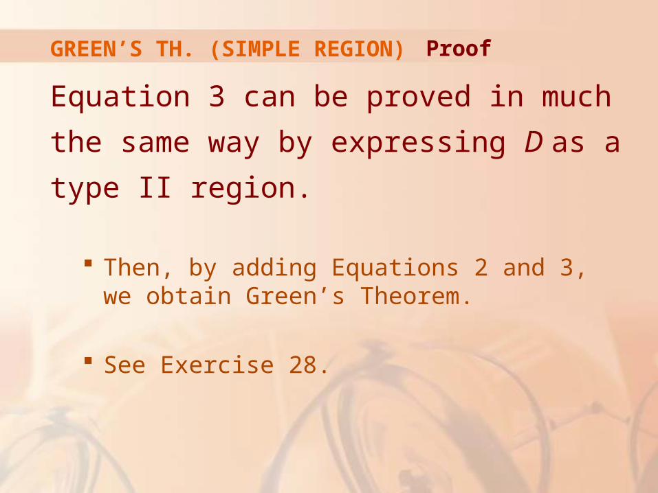
GREEN’S TH. (SIMPLE REGION)

Equation 3 can be proved in much the same

way by expressing D as a type II region.

Then, by adding Equations 2 and 3, we obtain Green’s Theorem.

See Exercise 28.

Proof

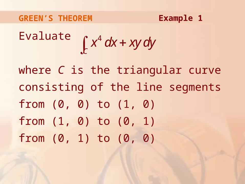
GREEN’S THEOREM

Evaluate

where C is the triangular curve

consisting of the line segments

from (0, 0) to (1, 0)

from (1, 0) to (0, 1)

from (0, 1) to (0, 0)

Example 1

4

Cx dx xy dy

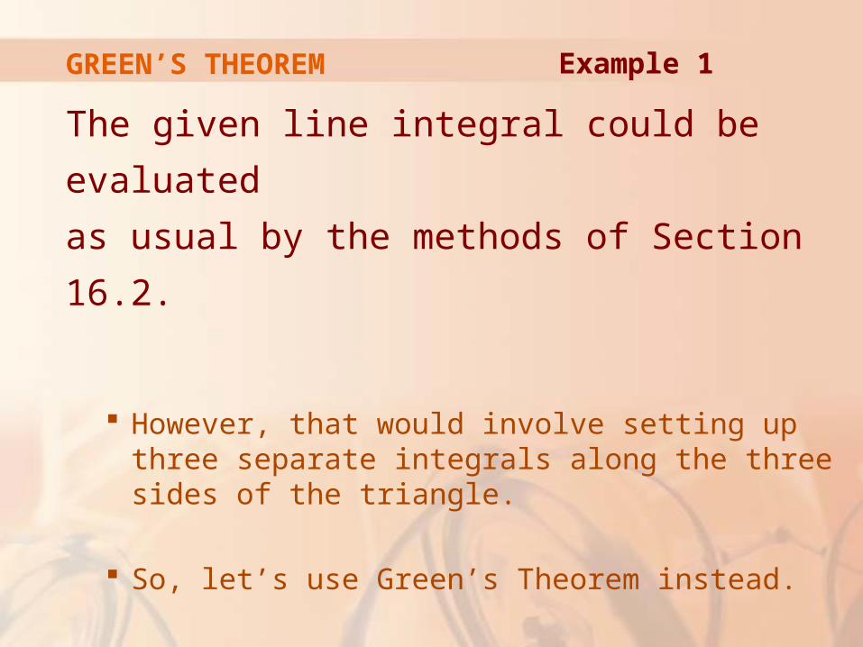
GREEN’S THEOREM

The given line integral could be evaluated

as usual by the methods of Section 16.2.

However, that would involve setting up three separate integrals along the three sides of the triangle.

So, let’s use Green’s Theorem instead.

Example 1

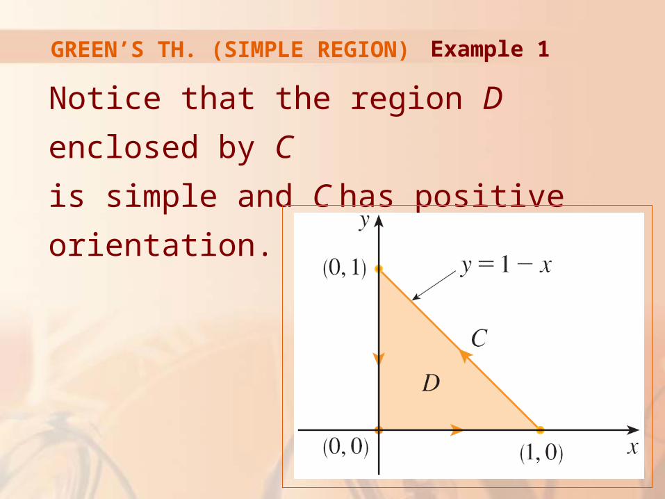
GREEN’S TH. (SIMPLE REGION)

Notice that the region D enclosed by C

is simple and C has positive orientation.

Example 1

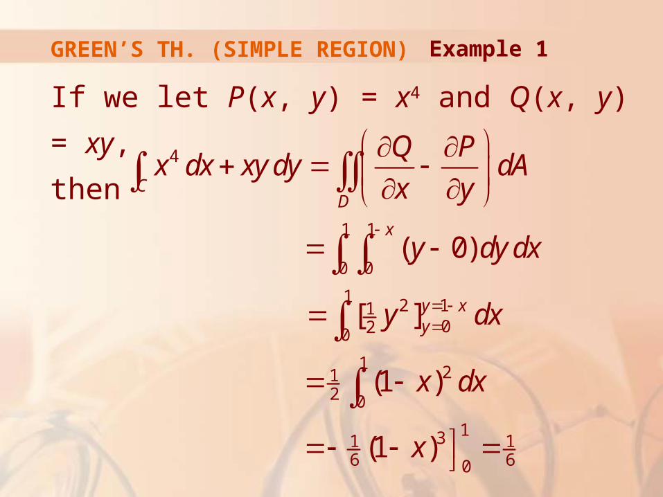
GREEN’S TH. (SIMPLE REGION)

If we let P(x, y) = x4 and Q(x, y) = xy,

then 4

1 1

0 0

1 2 11020

1 212 0

131 16 60

( 0)

[ ]

(1 )

(1 )

CD

x

y xy

Q Px dx xy dy dA

x y

y dy dx

y dx

x dx

x

Example 1

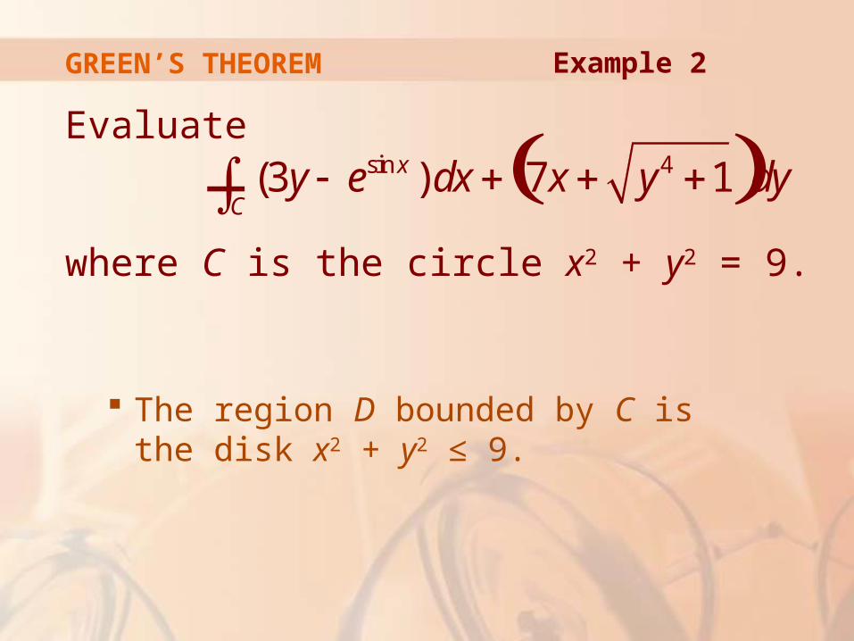
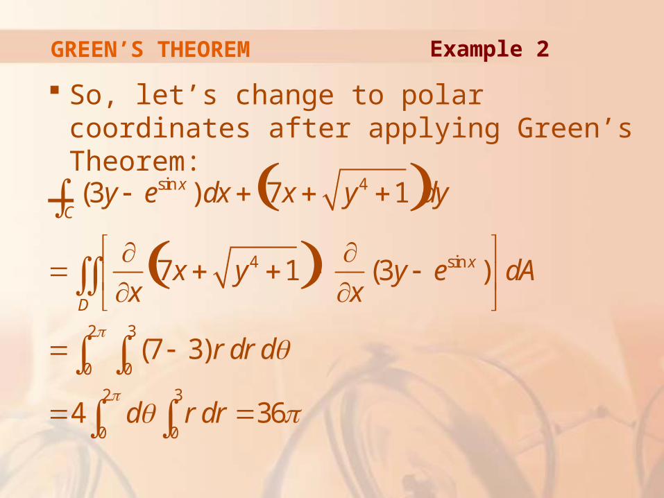
GREEN’S THEOREM

Evaluate

where C is the circle x2 + y2 = 9.

The region D bounded by C is the disk x2 + y2 ≤ 9.

Example 2

(3y esin x )dx 7x y4 1 dy

C—

GREEN’S THEOREM

So, let’s change to polar coordinates after applying Green’s Theorem:

(3y esin x )dx 7x y4 1 dyC—

x

7x y4 1 x

(3y esin x )

D dA

(7 3)r dr d0

3

0

2

4 d

0

2

r dr 360

3

Example 2

GREEN’S THEOREM

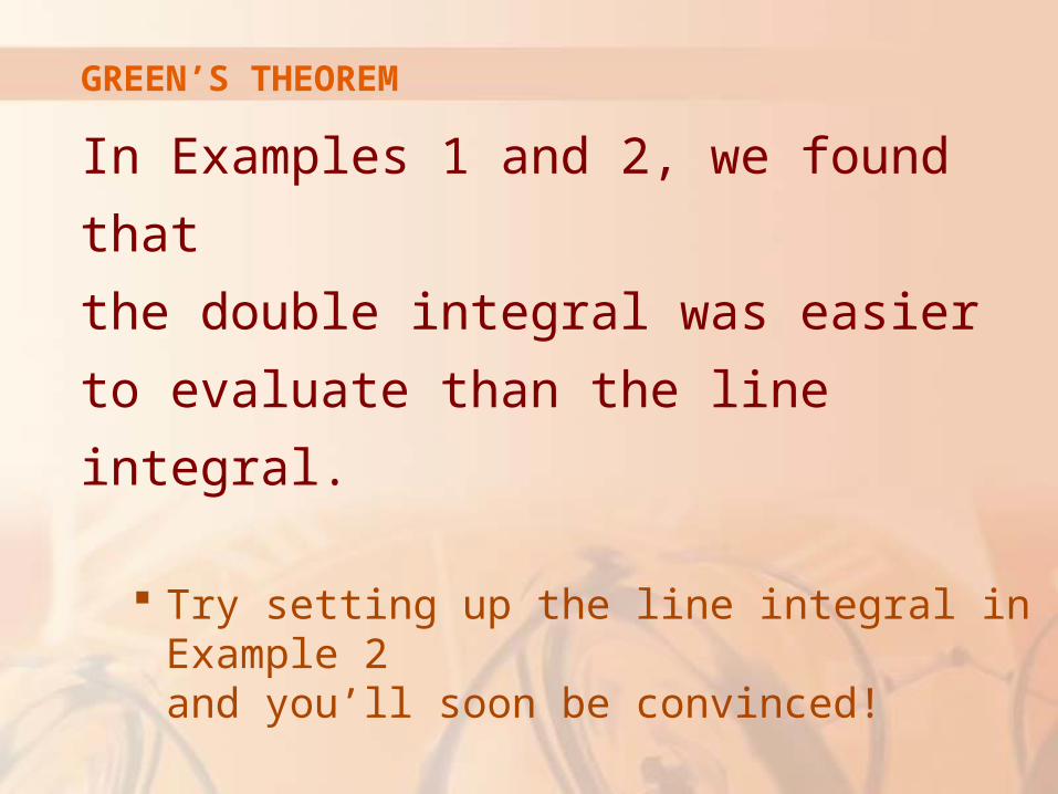
In Examples 1 and 2, we found that

the double integral was easier to evaluate

than the line integral.

Try setting up the line integral in Example 2 and you’ll soon be convinced!

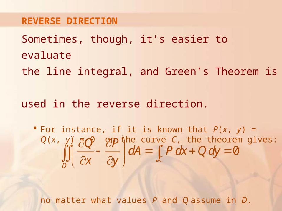
REVERSE DIRECTION

Sometimes, though, it’s easier to evaluate

the line integral, and Green’s Theorem is

used in the reverse direction.

For instance, if it is known that P(x, y) = Q(x, y) = 0 on the curve C, the theorem gives:

no matter what values P and Q assume in D.

0C

D

Q PdA P dx Q dy

x y

REVERSE DIRECTION

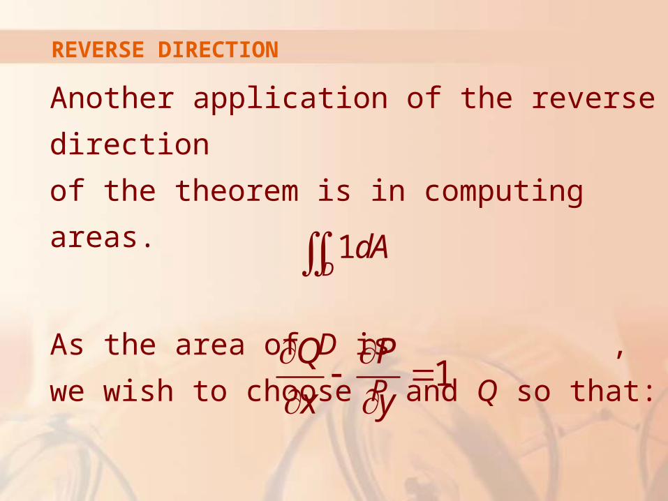
Another application of the reverse direction

of the theorem is in computing areas.

As the area of D is , we wish to choose

P and Q so that:

1D

dA

1Q P

x y

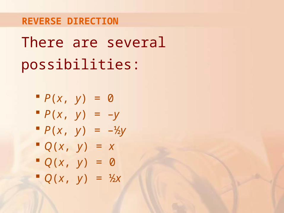
REVERSE DIRECTION

There are several possibilities:

P(x, y) = 0 P(x, y) = –y P(x, y) = –½y Q(x, y) = x Q(x, y) = 0 Q(x, y) = ½x

REVERSE DIRECTION

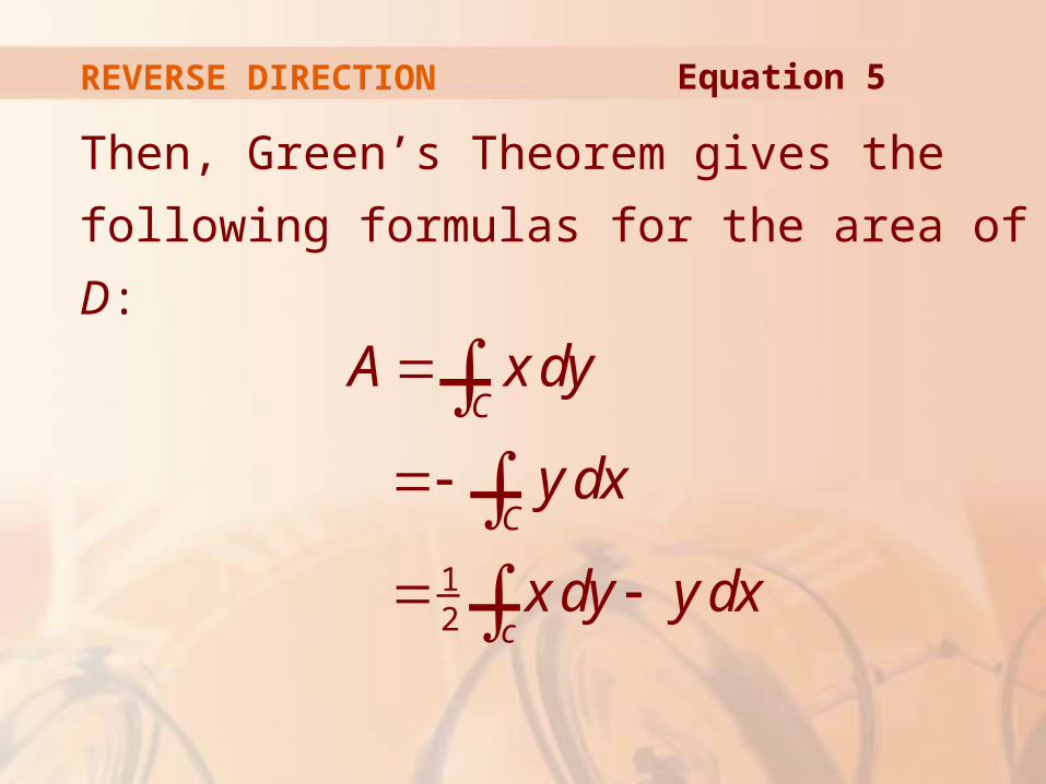
Then, Green’s Theorem gives the following

formulas for the area of D:

A x dyC—

yC— dx

12

x dy y dxc—

Equation 5

REVERSE DIRECTION

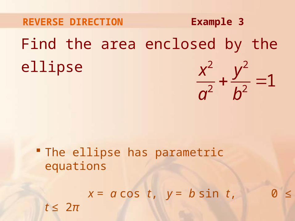
Find the area enclosed by the ellipse

The ellipse has parametric equations

x = a cos t, y = b sin t, 0 ≤ t ≤ 2π

Example 3

2 2

2 21

x y

a b

REVERSE DIRECTION

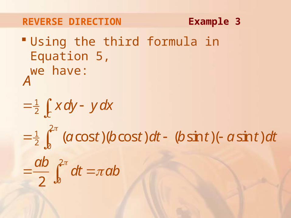
Using the third formula in Equation 5, we have:

12

212 0

2

0

( cos )( cos ) ( sin )( sin )

2

C

A

x dy y dx

a t b t dt b t a t dt

abdt ab

Example 3

UNION OF SIMPLE REGIONS

We have proved Green’s Theorem only

for the case where D is simple.

Still, we can now extend it to the case

where D is a finite union of simple regions.

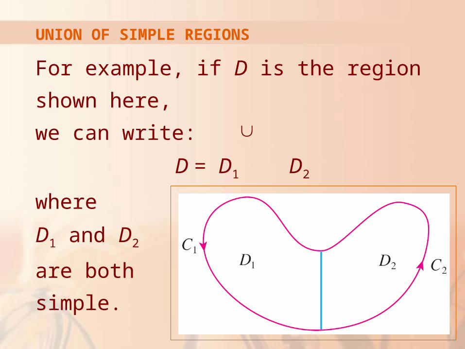
UNION OF SIMPLE REGIONS

For example, if D is the region shown here,

we can write:

D = D1 D2

where

D1 and D2

are both

simple.

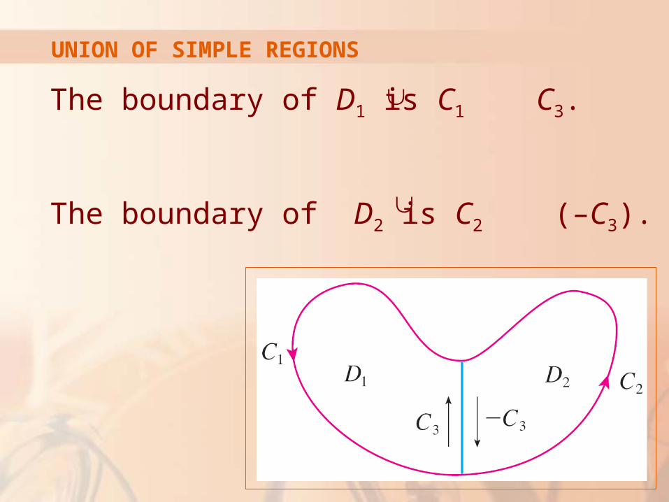
UNION OF SIMPLE REGIONS

The boundary of D1 is C1 C3.

The boundary of D2 is C2 (–C3).

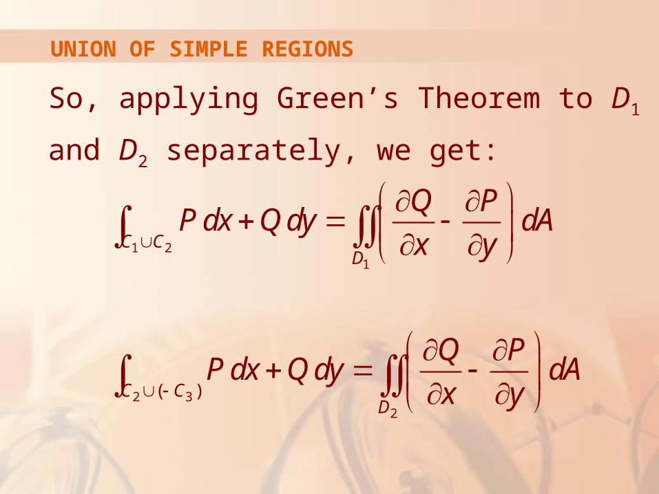
UNION OF SIMPLE REGIONS

So, applying Green’s Theorem to D1 and D2

separately, we get:

1 21

2 32

( )

C CD

C CD

Q PP dx Q dy dA

x y

Q PP dx Q dy dA

x y

UNION OF SIMPLE REGIONS

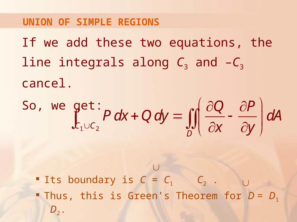
If we add these two equations, the line

integrals along C3 and –C3 cancel.

So, we get:

Its boundary is C = C1 C2 .

Thus, this is Green’s Theorem for D = D1 D2.

1 2C CD

Q PP dx Q dy dA

x y

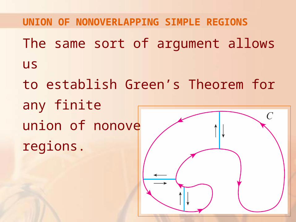
UNION OF NONOVERLAPPING SIMPLE REGIONS

The same sort of argument allows us

to establish Green’s Theorem for any finite

union of nonoverlapping simple regions.

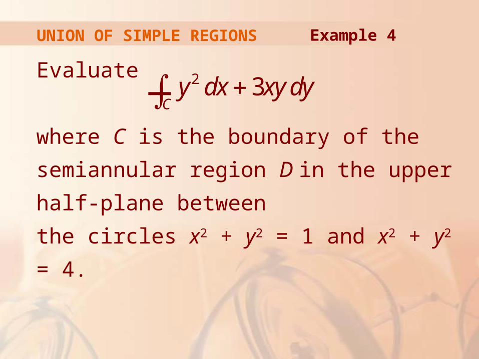
UNION OF SIMPLE REGIONS

Evaluate

where C is the boundary of the semiannular

region D in the upper half-plane between

the circles x2 + y2 = 1 and x2 + y2 = 4.

y2 dx 3xy dy

C—

Example 4

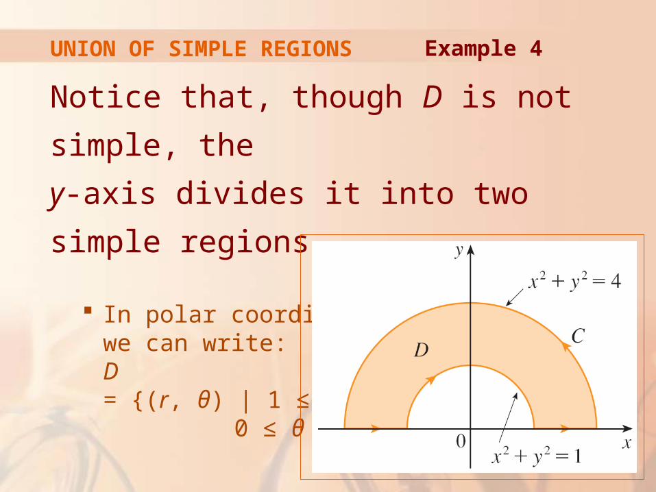
UNION OF SIMPLE REGIONS

Notice that, though D is not simple, the

y-axis divides it into two simple regions.

In polar coordinates, we can write: D = {(r, θ) | 1 ≤ r ≤ 2,

0 ≤ θ ≤π}

Example 4

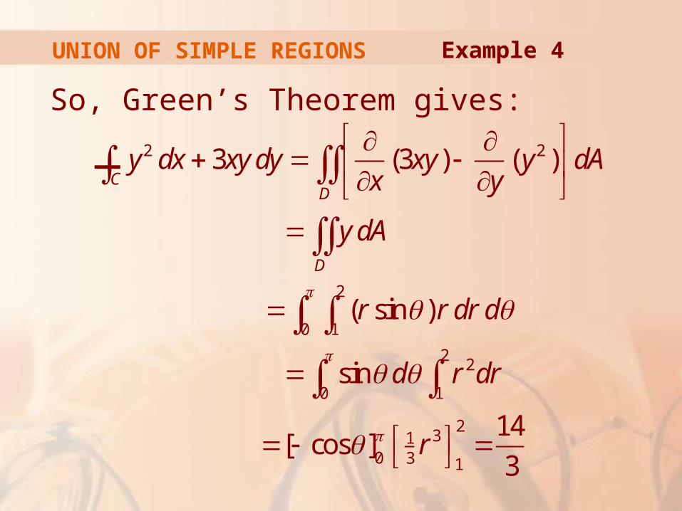
UNION OF SIMPLE REGIONS

So, Green’s Theorem gives:

y2 dxC— 3xy dy

x

(3xy) y

( y2 )

D dA

y dAD

(r sin)r dr d1

2

0

sin d

0

r 2dr1

2

[ cos]

0 1

3r3 1

2

14

3

Example 4

REGIONS WITH HOLES

Green’s Theorem can be extended

to regions with holes—that is, regions

that are not simply-connected.

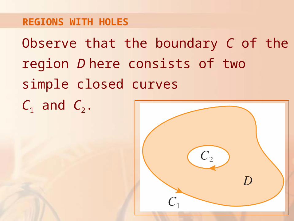
REGIONS WITH HOLES

Observe that the boundary C of the region D

here consists of two simple closed curves

C1 and C2.

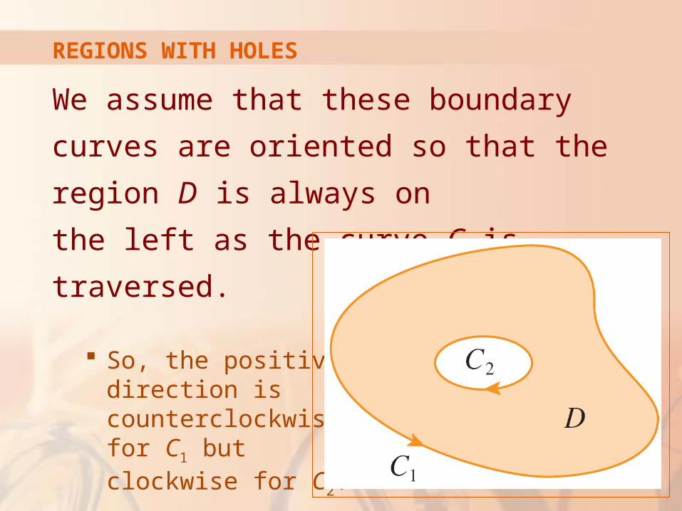
REGIONS WITH HOLES

We assume that these boundary curves are

oriented so that the region D is always on

the left as the curve C is traversed.

So, the positive direction is counterclockwise for C1 but clockwise for C2.

REGIONS WITH HOLES

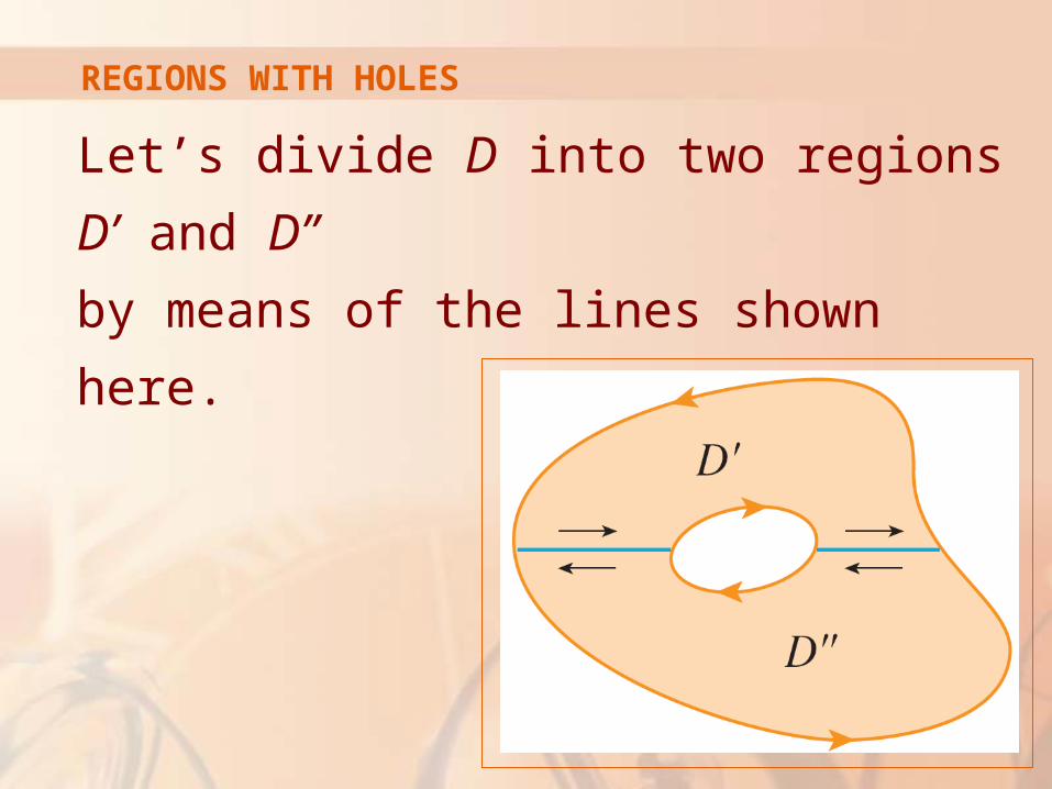
Let’s divide D into two regions D’ and D”

by means of the lines shown here.

REGIONS WITH HOLES

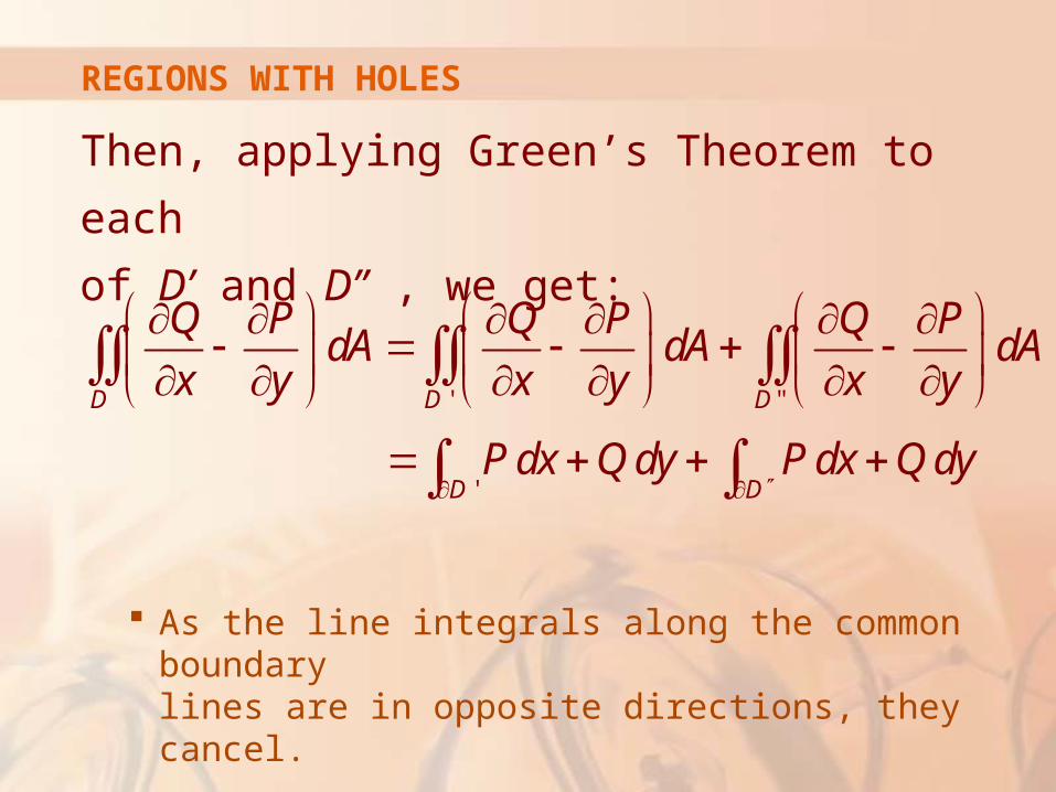
Then, applying Green’s Theorem to each

of D’ and D” , we get:

As the line integrals along the common boundary lines are in opposite directions, they cancel.

' "

'

D D D

D D

Q P Q P Q PdA dA dA

x y x y x y

P dx Q dy P dx Q dy

REGIONS WITH HOLES

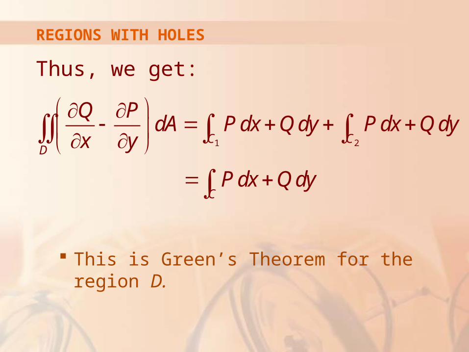
Thus, we get:

This is Green’s Theorem for the region D.

1 2C CD

C

Q PdA P dx Q dy P dx Q dy

x y

P dx Q dy

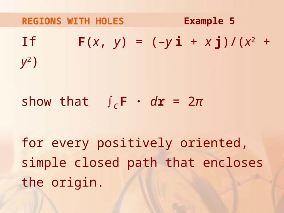
REGIONS WITH HOLES

If F(x, y) = (–y i + x j)/(x2 + y2)

show that ∫C F · dr = 2π

for every positively oriented, simple closed

path that encloses the origin.

Example 5

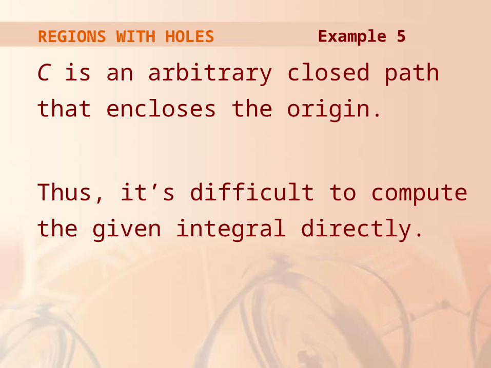
REGIONS WITH HOLES

C is an arbitrary closed path that encloses

the origin.

Thus, it’s difficult to compute the given

integral directly.

Example 5

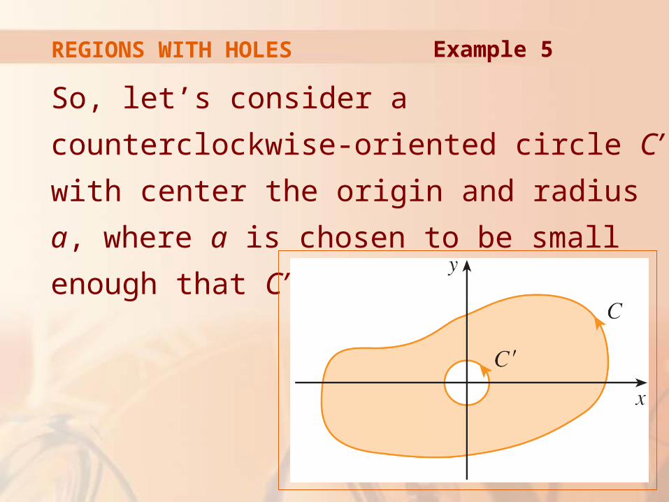
REGIONS WITH HOLES

So, let’s consider a counterclockwise-oriented

circle C’ with center the origin and radius a,

where a is chosen to be small enough that C’

lies inside C.

Example 5

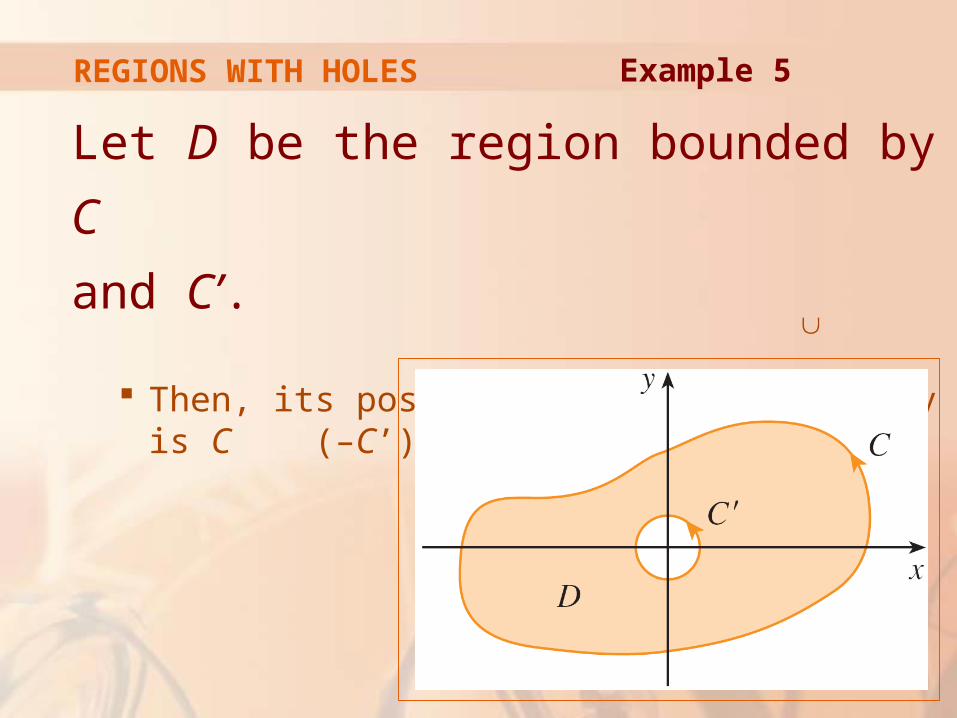
REGIONS WITH HOLES

Let D be the region bounded by C

and C’.

Then, its positively oriented boundary is C (–C’).

Example 5

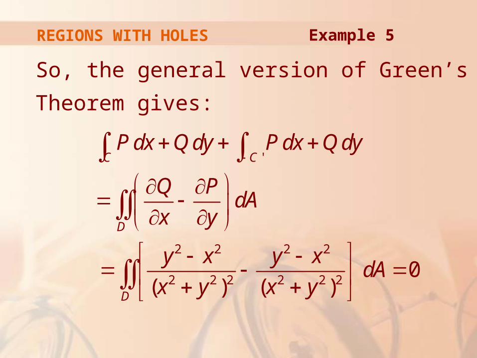
REGIONS WITH HOLES

So, the general version of Green’s Theorem

gives:

'

2 2 2 2

2 2 2 2 2 20

( ) ( )

C C

D

D

P dx Q dy P dx Q dy

Q PdA

x y

y x y xdA

x y x y

Example 5

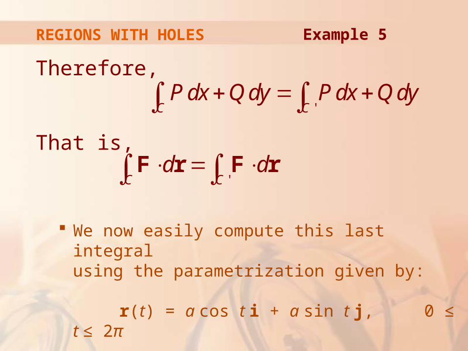
REGIONS WITH HOLES

Therefore,

That is,

We now easily compute this last integral using the parametrization given by:

r(t) = a cos t i + a sin t j, 0 ≤ t ≤ 2π

'C CP dx Q dy P dx Q dy

'C Cd d F r F r

Example 5

REGIONS WITH HOLES

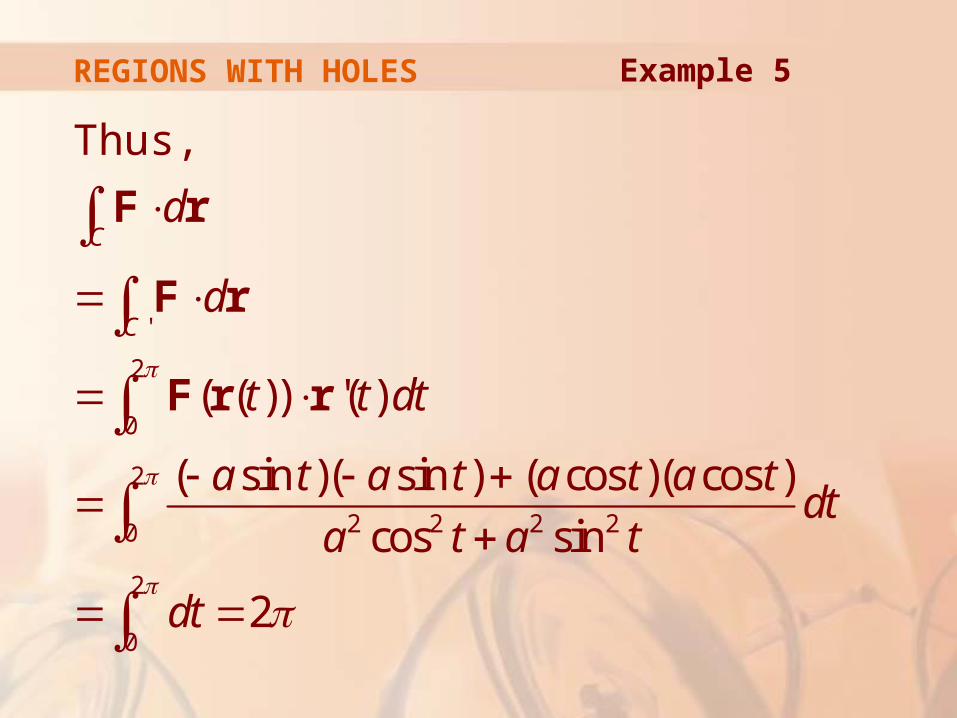
Thus,

Example 5

'

2

0

2

2 2 2 20

2

0

( ( )) '( )

( sin )( sin ) ( cos )( cos )

cos sin

2

C

C

d

d

t t dt

a t a t a t a tdt

a t a t

dt

F r

F r

F r r

GREEN’S THEOREM

We end by using Green’s Theorem

to discuss a result that was stated in

Section 16.3

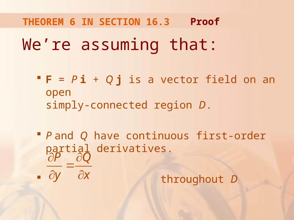
THEOREM 6 IN SECTION 16.3

We’re assuming that:

F = P i + Q j is a vector field on an open simply-connected region D.

P and Q have continuous first-order partial derivatives.

throughout D

Proof

P Q

y x

THEOREM 6 IN SECTION 16.3

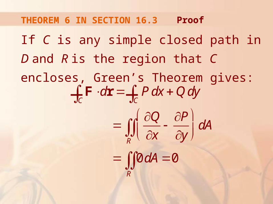
If C is any simple closed path in D and R is

the region that C encloses, Green’s Theorem

gives:

FdrC— P dx Q dy

C—

Q

x

P

y

R

dA

0 dAR 0

Proof

THEOREM 6 IN SECTION 16.3

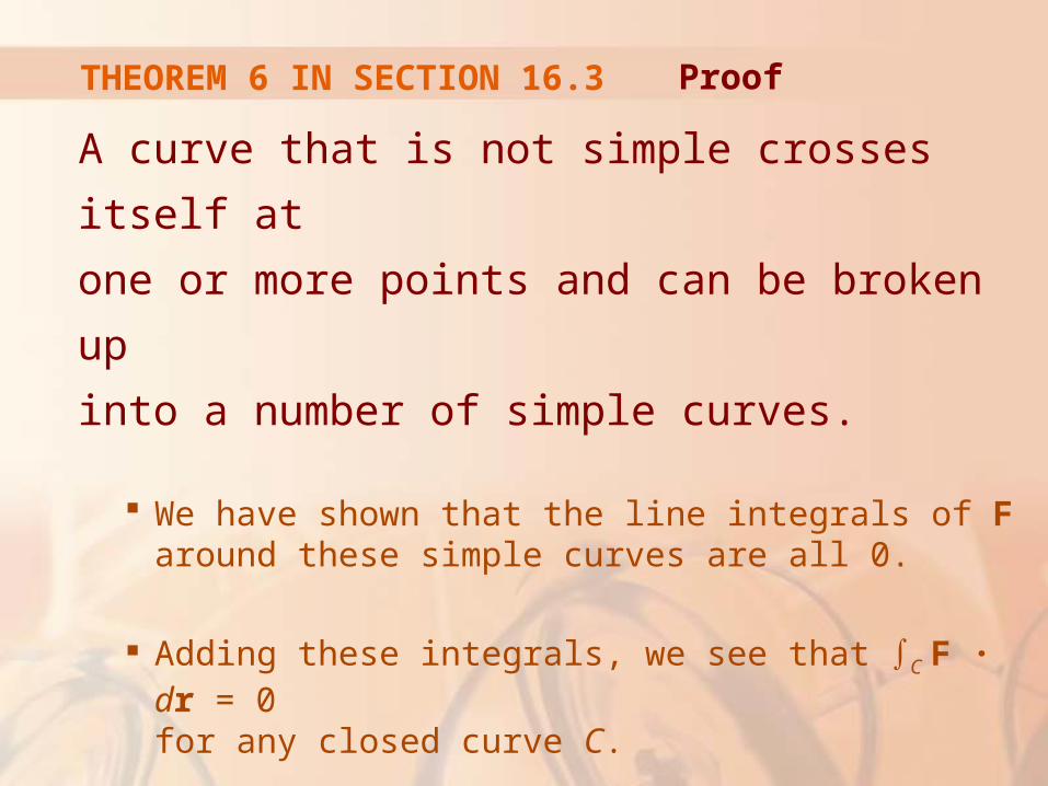
A curve that is not simple crosses itself at

one or more points and can be broken up

into a number of simple curves.

We have shown that the line integrals of F around these simple curves are all 0.

Adding these integrals, we see that ∫C F · dr = 0 for any closed curve C.

Proof

THEOREM 6 IN SECTION 16.3

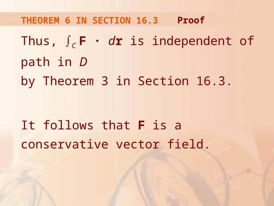
Thus, ∫C F · dr is independent of path in D

by Theorem 3 in Section 16.3.

It follows that F is a conservative vector field.

Proof