variations in stratospheric inorganic chlorine between ... · variations in stratospheric inorganic...

Source of Acquisition NASA Goddald Space Flight Center

POPULAR SUMMARY

Variations in Stratospheric Inorganic Chlorine Between 1991 and 2006

D.J. Lary, D.W. Waugh, A.R. Douglass, R.S. Stolarski, P.A. Newman, H. Mussa

So how quickly will the ozone hole recover? This depends on how quickly the chlorine content ((21,) of the atmosphere will decline. The ozone hole forms over the Antarctic each southern spring (September and October). The extremely small ozone amounts in the ozone hole are there because of chemical reactions of ozone with chlorine. This chlorine originates largely from industrially produced chlorofluorocarbon (CFC) compounds. An international agreement, the Montreal Protocol, is drastically reducing the amount of chlorine-containing compounds that we are releasing into the atmosphere.

To be able to attribute changes in stratospheric ozone to changes in chlorine we need to know the distribution of atmospheric chlorine. However, due to a lack of continuous observations of all the key chlorine gases, producing a continuous time series of stratospheric chlorine has not been achieved to date. We have for the first time devised a technique to make a 17-year time series for stratospheric chlorine that uses the long time series of HCI observations made from several space borne instruments and a neural network. The neural networks allow us to both inter-calibrate the various HCI instruments and to infer the total amount of atmospheric chlorine from HCl. These new estimates of C1, provide a much needed critical test for current global models that currently predict significant differences in both C1, and ozone recovery. These models exhibit differences in their projection of the recovery time and our chlorine content time series will help separate the good from the bad in these projections.

https://ntrs.nasa.gov/search.jsp?R=20070030220 2019-02-07T13:28:32+00:00Z

GEOPHYSICAL RESEARCH LETTERS, VOL. ???, XXXX, DOI:10.1029/,

Variations in Stratospheric Inorganic Chlorine Between 1991 and 2006 D.J. ~ a r ~ ' ' ~ , D.W. waugh3, A.R. ~ o u ~ l a s s ' , R.S. sto1arski2, P.A. ~ e w m a n ~ ,

D. J. Lary, Goddard Earth Sciences and Technology Centre, University of Maryland Baltimore

County, Baltimore, MD 21228 ([email protected])

'Goddard Earth Sciences and Technology

Centre, University of Maryland Baltimore

County, Baltimore, Maryland, USA

2Atmospheric Chemistry and Dynamics

Branch, NASA, Goddard Space Flight

Centre, Greenbelt, Maryland, USA

3The Department of Earth & Planetary

Sciences Maryland, Johns Hopkins

University, Baltimore, USA

4Department of Chemistry, University of

Cambridge, England

April 11, 2007, 3:27pm D R A F T

X - 2 LARY E T AL.: STRATOSPHERIC CHLORINE FROM 1991-2006

A consistent time series of stratospheric inorganic chlorine C1, from 1991

to present is formed using space-borne observations together with neural net-

5 works. A neural network is first used to account for inter-instrument biasses

6 in HC1 observations. A second neural network is used to learn the abundance

of Cly as a function of HC1 and CH4, and to form a time series using avail-

* able HC1 and CH4 measurements. The estimates of C1, are broadly consis-

tent with calculations based on tracer fractional releases and previous esti-

mates of stratospheric age of air. These new estimates of C1, provide a crit-

ical test for current global models that predict significant differences in C1,

12 and ozone recovery.

D R A F T April 11, 2007, 3:27pm D R A F T

LARY ET AL.: STRATOSPHERIC CHLORINE FROM 1991-2006 X - 3

1. In t roduct ion

13 Knowledge of the distribution of inorganic chlorine C1, in the stratosphere is needed to

14 attribute changes in stratospheric ozone to changes in halogens, and to assess the realism

15 of chemistry-climate models [Eyring et al., 2006; Eyring, 20071. However, there are limited

16 direct observations of Cl,. Simultaneous measurements of the major inorganic chlorine

17 species are rare [Zander et al., 1992; Gunson et al., 1994; Bonne et al., 2000; Nassar et al.,

18 20061. In the upper stratosphere, Cly can be inferred from HC1 alone (e.g., Anderson et al.

19 [2000]).

20 Here we combine observations from several space-borne instruments using neural net-

21 works [Lary and Mussa, 20041 to produce a time series for Cl,. A neural network is used

22 to characterize differences among various HC1 measurements, and to perform an inter-

23 instrument bias correction. Measurements from several different instruments are used in

24 this analysis. These instruments, together with temporal coverage and measurement un-

25 certainties, are listed in Table 1. All instruments provide measurements through the depth

26 of the stratosphere. A second neural network is used to infer Cly from these corrected

27 HC1 measurements and measurements of CH4.

28 Sections 2 and 3 describe the HC1 and C1, intercomparisons. Section 4 present a sum-

29 mary.

2. HCI Intercomparison

30 We first compare measurements of HCl from different instruments listed in Table 1.

31 Conlparisons are made in equivalent PV latitude - potential temperature coordinates

32 [Schoeberl et al., 1989; Profitt et al., 1989; Lait et al., 1990; Douglass et al., 1990; Lary



33 e t al., 1995; Schoeberl et al., 20001 to extend the effective latitudinal coverage of the

34 measurements and identify contemporaneous measurements in similar air masses.

35 The Halogen Occultation Experiment (HALOE) provides the longest record of space

36 based HC1 observations. Figure 1 compares HALOE HC1 with HC1 observations from

37 (a) the Atmospheric Trace Molecule Spectroscopy Experiment (ATMOS), (b) the Atmo-

38 spheric Chemistry Experiment (ACE) and (c) the Microwave Limb Sounder (MLS). In

30 these plots each point is the median HC1 observation made by the instrument during each

40 month for 30 equivalent latitude bins from pole to pole and 25 potential temperature bins

41 from the 300-2500 K potential temperature surfaces.

42 A consistent picture is seen in these plots: HALOE HC1 measurements are lower than

43 those from the other instruments. The slopes of the linear fits (relative scaling) are

44 1.05 for the HALOE-ATMOS comparison, 1.09 for the HALOE-MLS, and 1.18 for the

45 HALOE-ACE. The offsets are apparent at the 525 K isentropic surface and above. Pre-

46 vious comparisons among HCl datasets reveal a similar bias for HALOE [Russell et al.,

47 1996; MeHugh et al., 2005; Froidevaux et al., 20061. ACE and MLS HCl measurements are

48 in much better agreement [Figure l(d)]. Note, all measurements agree within the stated

49 observational uncertainties summarized in Table 1.

50 To combine the above HC1 measurements to form a continuous time series of HC1 (and

51 then Cl,) from 1991 to 2006 it is necessary to account for the baises between data sets. A

52 neural network is used to learn the mapping from one set of nieasurements onto another as

53 a function of equivalent latitude and potential temperature [Lary and Mussa, 20041. We

54 consider two cases. In one case ACE HCl is taken as the reference and the HALOE and

D R A F T A p r i l 11, 2007, 3:27pm D R A F T

LARY E T AL.: STRATOSPEIERIC CHLORTNE FROM 1991-2006 X - 5

55 Aura HCl observations are adjusted to agree with ACE HC1. In the other case HALOE

56 HC1 is taken as the reference and the Aura and ACE HC1 observations are adjusted to agree

57 with HALOE HC1. In both cases we use equivalent latitude and potential temperature

58 to produce average profiles. The purpose of the mapping is simply to learn the bias as a

59 function of location, not to imply which instrument is correct.

The precision of the correction using the neural network mapping is of the order of %

61 0.3 ppbv, as seen in Figure l(e) which shows the results when HALOE HC1 measurements

62 have been mapped into ACE measurements. The mapping has removed the bias between

63 the measurements and has also straightened out the 'wiggles' in 1 (c), i.e., the neural

64 network has learned the equivalent PV latitude and potential temperature dependence

65 of the bias between HALOE and MLS. The inter-instrument offsets are not constant in

66 space or time, and are not a simple function of C1,

3. Inorganic Chlorine C1,

67 TO a first approximation C1, % HC1 + C10N02 + C10 [Brasseur and Solomon, 19871,

M( and Cly can be estimated from HC1 and C10N02. However, observations of C10N02 are

69 much more limited than from HC1. As shown in Table 1, C10N02 measurements have

70 been made by the CLAES (1991-1993), ATMOS (1992-1994), CRISTA (1994, 1998)) and

71 ACE (2004-present).

72 Because of the limited temporal coverage of C10N02 measurements it is not possible

73 to form a coiitinuous time series of C1, by combining HC1, C10N02, and C10. However,

74 it is possible to form a time series of C1, using a neural network. There are sufficient

T5 observations of C10N02 from ATMOS, CLAES, CRISTA, and ACE to train a neural

D R A F T Apr i l 11, 2007, 3:27pm D R A F T

X - 6 LARY E T AL.: STRATOSPHERIC CI-ILORINE FROM 1991-2006

76 network to learn the C1, abundance as a function of HC1 and CH4, for each of which there

77 is a long, near-continuous, time series of measurements. The resulting reconstruction

78 reproduces an independent validation dataset faithfully with a correlation coefficient of

79 0.99, and provides a scatter diagram with a slope very close to one for the observed C1,

plotted against the neural network inferred Cl,, see Figure l(f).

81 The inputs to the neural network that estimates C1, are HC1, CH4, equivalent latitude

82 and potential temperature. HCl is used because it is continuously observed from the

83 launch of UARS to the present and is typically the major C1, reservoir. CH4 is used

84 because it is continuously observed from the launch of UARS to the present and, as a

85 long-lived tracer, it is well correlated with Cl,. Potential temperature and equivalent

86 latitude are used because the correlation between long-lived tracers such as CH4 and C1,

87 is a strong function of altitude and a weak function of latitude [Lary and Mussa, 20041.

88 Other training strategies using more species were examined. For example, we tested

89 the effectiveness of a neural network with inputs of HC1, 03, CHq, H 2 0 , equivalent

90 latitude and potential temperature to estimate Cl,. This was tried as 03, CH4 and HzO

91 are key observed species involved in the partitioning of reactive chlorine. When chlorine

92 atoms are released from the chlorine containing source gases by photolysis, they react

93 with CH4 to form HC1. Alternatively, C1 atoms may react with ozone to form C10, and

94 then C10 will combine with NO2 to form C10N02. HC1 is destroyed either by reaction

95 with OH, photolysis or heterogeneous reactions. The amount of OH present depends on

96 the photolysis of ozone to form O('D) and the subsequent reaction of 0('D) with H20.


LARY E T AL.: STRATOSPHERIC CHLORlNE FROM 1991-2006 X - 7

Q7 This approach also gave good results, but with slightly lower skill than just using HC1,

98 CH4, equivalent latitude and potential temperature to estimate '21,.

99 Figure 2 shows how C1, profiles estimated by the neural network agree with observed

lw C1, for October 2006. In each case the shaded range represents the uncertainty associated

101 with the C1, estimate. We note that the HC1 bias between HALOE and ACE is the major

102 uncertainty.

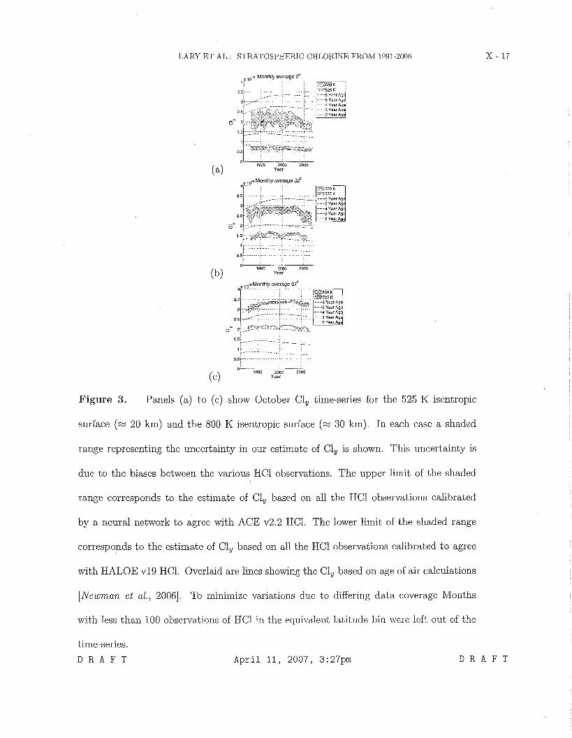
lo3 The distribution of C1, is expected to change between 1991 and 2006 as the abundances

1M of its source gases have changed. Figure 3 shows the time-series of Cl, for the 525 K

105 isentropic surface (z 20 km) and the 800 K isentropic surface (z 30 km), for three

1% different equivalent latitudes. The upper limit of each shaded range corresponds to the

107 estimate of C1, for the neural network calibrated to agree with ACE v2.2 HC1, and the

108 lower limit to the estimate of C1, for the neural network calibrated to agree with HALOE

109 v19 HC1.

110 The variation in Cl, estimates between the two cases depends on latitude, altitude

111 and season and is typically 50.4 ppbv at 800 K. This uncertainty is primarily due to

112 the discrepancy between the different observations of HC1 which translates into the C1,

113 uncertainty shown by the shading in Figure 3. There is also a slight low bias in the lower

114 stratosphere due to not including HOCl in the estimates of Cl,. HOCl was not included

115 because HOCl has been observed by ACE only since the start of 2004. Ignoring HOCl

115 is only of significance in regions of strong chlorine activation a t low temperatures in the

117 lower stratosphere where HOCl can comprise up-to about 10% of Cl,.


X - 8 LARY ET AL.. STRATOSPHERIC CHLORINE FROM 1991-2006

118 There is a general tendency of C1, to increase in the 1990s, peak around 2000, and

119 then slowly decrease. This is consistent with our expectations based on the tropospheric

120 abundence of chlorine containing source gases. The C1, time-series shown in Figure 3

121 constitutes a useful test for model simulations. The variation in simulated Cl, from the

122 chemistry-climate models used in the recent WM0 [2006] report is much greater than

123 the above uncertainty in Cl,. For example, the simulated peak C1, in October a t 80s

124 varies from less than 1 ppbv to over 3.5 ppbv, while the peak annual-mean Cl, for north

125 mid-latitudes varies from 0.8 to 2.8 ppb [Eyrzng et al., 2006; Eyrzng, 20071.

126 The estimates of C1, produced are broadly consistent with calculations based on tracer

127 fractional releases [Newman et al., 20061 and previous estimates of stratospheric age of

128 air. Observations show that at 20 km the mean age increases from around 2 years in

12g the tropics to around 4 years at high latitudes (60°N), with a similar gradient at 30 km

130 but older ages by around 2 years [Waugh and Hall, 20021. The curves in Figure 3 show

131 calculations of C1, for a range values of the mean age of air, and the ages that are required

132 to match the observed C1, are consistent with the observations of the mean age.

4. Summary

133 A consistent time series of stratospheric C1, from 1991 to present has been formed

1 3 using available space-borne observations. Here we used neural networks to inter-calibrate

135 KC1 measurements from different instruments, and to estimate C1, from observations

136 of HC1 and CH4. These estimates of C1, peaked in the late 1990s and have begun to

137 decline as expected from tropospheric measurements of source gases and troposphere to

stratosphere transport times. Furthermore, the estimates of C1, produced are consistent

Apr i l 11, 2007, 3:27pm

LARY ET AL.: STRATOSPHEFUC CHLORINE FROM 1991-2006 X - 9

139 with calculations based on tracer fractional releases and age of air [ N e w m a n et al., 20061.

140 The C1, time-series formed here is an important benchmark for models being used to

141 simulate the recovery of the ozone hole. Although there is uncertainty in the estimates

142 of CIY, primarily due to biases in HC1 measurements, this uncertainity is small conipared

143 with the range of model predictions shown in the recent WMO [2006] report. The two

144 CIY time-series are available in the electronic supplement.

145 Acknowledgments. It is a pleasure to acknowledge NASA for research funding, Lu-

146 cien Froidevaux and the Aura MLS team for their data, the ACE team, Peter Bernath,

141 Chris Boone, and Kaley Wallter for their data, the HALOE team and Ellis Remsberg for

148 their data, and the ATMOS team for their data. The ACE mission is funded primarily

149 by the Canadian Space Agency.



References

1% Anderson, J., J . M. Russell, S. Solomon, and L. E. Deaver, Halogen occultation experi-

151 ment confirmation of stratospheric chlorine decreases in accordance with the montreal

152 protocol, J. Geophys. Res. (Atmos.), 105 (D4), 4483-4490, 2000.

153 Bernath, P. F., et al., Atmospheric chemistry experiment (ace): Mission overview, Geo-

154 phys. Res. Lett., 32(15), 115S01, 2005.

155 Bonne, G. P., et al., An examination of the inorganic chlorine budget in the lower strato-

156 sphere, J. Geophys. Res. (Atmos.), 105(D2), 1957-1971, 2000.

157 Brasseur, G., and S. Solomon, Aeronomy of the Middle Atmosphere : Chemistry and

158 Physics of the Stratosphere and Mesosphere, Atmospheric Science Library, second ed.,

159 D Reidel Pub Co, 1987.

1 ~ ) Douglass, A., R. Rood, R. Stolarski, M. Schoeberl, M. Proffitt, J. Margitan, M. Loewen-

161 stein, J. Podolske, and S. Strahan, Global 3-dimensional constituent fields derived from

162 profile data, Geophys. Res. Lett., 17(4 SS), 525-528, 1990.

163 Eyring, V., et al., Assessment of temperature, trace species, and ozone in chemistry-

IM climate model simulations of the recent past, J. Geophys. Res. (Atmos.), I l l (D22),

165 2006.

166 Eyring, V. e. a., Multi-model projections of stratospheric ozone in the 21st century, J.

167 Geophys. Res. (Atmos.), submitted, 2007.

168 Froidevaux, L., et al., Early validation analyses of atmospheric profiles from EOS MLS

169 on the aura satellite, IEEE Trans. Geosci. Remote Sens., 44 (5), 1106-1 121, 2006.

April 11, 2007, 3:27pm

LARY E T AL.: STRATOSPHERIC CHLORINE FROM 1991-2006 X - 11

170 Gunson, M. R., M. C. Abrams, L. L. Lowes, E. Mahieu, R. Zander, C. P. Rinsland,

171 M. K. W. KO, N. D. Sze, and D. K. Weisenstein, Increase in levels of stratospheric

172 chlorine and fluorine loading between 1985 and 1992, Geophys. Res. Lett., 21 (20), 2223-

173 2226, 1994.

174 Lait, L., et al., Reconstruction of O3 and N20 fields from ER-2, DC-8, and balloon obser-

175 vations, Geophys. Res. Lett., 17(4 SS), 521-524, 1990.

176 Lary, D., M. Chipperfield, J. Pyle, W. Norton, and L. Riishojgaard, 3-dimensional

177 tracer initialization and general diagnostics using equivalent PV latitude-potential-

178 temperature coordinates, Q. J. R. Meteorol. Soc., 121 (521 PtA) , 187-210, 1995.

179 Lary, D. J . , and H. Y. Mussa, Using an extended kalman filter learning algorithm for

180 feed-forward neural networks to describe tracer correlations, Atmospheric Chemistry

181 and Physics Discussions, 4, 3653-3667, 2004.

182 McHugh, M., B. Magill, K. A. Walker, C. D. Boone, P. F. Bernath, and J . M. Russell,

183 Comparison of atmospheric retrievals from ace and haloe, Geophys. Res. Lett., 32(15),

18, 0094-8276 L15S10, 2005.

185 Nassar, R., et.al., A global inventory of stratospheric chlorine in 2004, J. Geophys. Res.

186 (Atmos.), 111 (D22), 0148-0227 D22312, 2006.

187 Newman, P. A., E. R. Nash, S. R. Kawa, S. A. Montzka, and S. M. Schauffler, When will

188 the antarctic ozone hole recover?, Geophys. Res. Lett., 33(12), 2006.

189 Offermann, D., K. U. Grossmann, P. Barthol, P. Knieling, M. Riese, and R. Trant, Cryo-

190 genic infrared spectrometers and telescopes for the atmosphere (crista) experiment and

191 middle atmosphere variability, J. Geophys. Res. (Atmos.), lO4(Dl3), 16,311-16,325,

D R A F T April 11, 2007, 3:27pm

X - 1 2 LARY E T AL.: STRATOSPHERIC CHLORINE FROM 1991-2006

192 1999.

193 Proffitt, M., et al., Insitu ozone measurements within the 1987 antarctic ozone hole from a

194 high-altitude ER-2 aircraft, J. Geophys. Res. (Atmos.), 94(D14), 16,547-16,555, 1989.

195 Roche, A. E., J . B. Kumer, J. L. Mergenthaler, G. A. Ely, W. G. Uplinger, J. F. Pot-

196 ter, T. C. James, and L. W. Sterritt, The cryogenic limb array etalon spectrometer

197 (CLAES) on UARS - experiment description and performance, J. Geophys. Res. (At-

198 mos.), 98(D6), 10,763-10,775, 1993.

1g9 Russell, J . M., et al., The Halogen Occultation Experiment, J. Geophys. Res. (Atmos.),

2m 98(D6), 10,777-10,797, 1993.

201 Russell, J. M., et al., Validation of hydrogen chloride measurements made by the halogen

202 occultation experiment from the UARS platform, J. Geophys. Res. (Atmos.), 101 (D6),

203 10,151-10,162, 0148-0227, 1996.

204 Schoeberl, M. R., L. C. Sparling, C. H. Jackman, and E. L. Fleming, A lagrangian view of

205 stratospheric trace gas distributions, J. Geophys. Res. (Atmos.), 105(D1), 1537-1552,

206 2000.

207 Schoeberl, M. R., et al., Reconstruction of the constituent distribution and trends in

208 the antarctic polar vortex from er-2 flight observations, J. Geophys. Res. (Atmos.),

209 94 (D14), 16,815-16,845, 1989.

210 Waugh, D., and T. Hall, Age of stratospheric air: theory, observations, and models,

211 Reviews of geophysics, 2000RG000101(10.1029), 2002.

212 WMO, Scientific assessment of ozone depletion: 2006, Tech. Rep. 50, WMO Global Ozone

213 Res. and Monitor. Proj., Geneva, 2006.


LARY E T AL.: STRATOSPHERIC CHLORINE FROM 1991-2006 X - 13

214 Zander, R., M. R. Gunson, C. B. Farmer, C. P. Rinsland, F. W. Irion, and E. Mahieu, The

215 1985 chlorine and fluorine inventories in the stratosphere based on atmos observations

216 at 30-degrees north latitude, J. Atmos. Chem., 15(2), 171-186, 1992.


LARY ET AL.: STRATOSPHERIC CHLORINE FROM 1991-2006

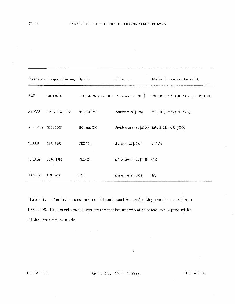
Instrument Temporal Coverage Species References Median Observation Uncertainty

ACE 2004-2006 HCI, CION02 and C10 Bernath et al. [2005] 8% (HCl), 30% (ClON02), >loo% (C10)

ATMOS 1991, 1993, 1994 HC1, ClONOz Zander et al. [I9921 8% (HCl), 60% (ClON02)

Aura MLS 2004-2006 HC1 and C10 Froidevaux et al. [2006] 12% (HCl), 76% (C10)

CLAES 1991-1993 ClONOz Roche et al. [I9931 > 100%

CRISTA 1994, 1997 ClON02 Oflermann et al. [I9991 61%

HALOE 1991-2005 HCI Russell et al. [I9931 4%

Table 1. The instruments and constituents used in constructing the C1, record from

1991-2006. The uncertainties given are the median uncertainties of the level 2 product for

all the observations made.

D R A F T Apri l 11, 2007, 3:27pm D R A F T

LARY E T AL.: STRATOSPHERIC CHLORINE FRORiI 1991-2006 X - 15

O 1 2 3 4 O 0 1 2 3 4

(a) HALOE HCI (ppbv) (b) HALOE HCl (ppbv) (4 HALOE HCI (ppbv)

5

3 if 4

P ;ii a, n a c

a 2 j- 3

- 0 d I 2 2 f: a 2 1

- 6 1

0 0 0 1 2 3 0 1 2 3 4 5

(4 MLS HCl (ppbv) (4 HALOE HCI (ppbv) NN adjusted ( f )

Targets T

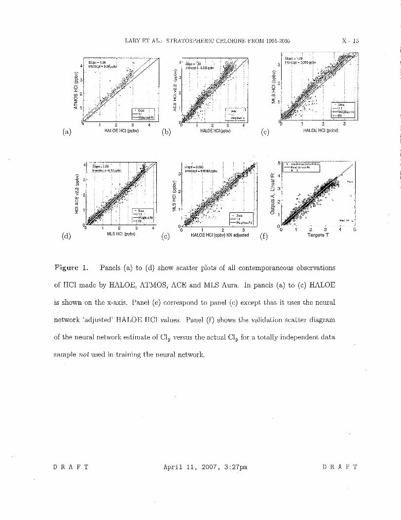
Figure 1. Panels (a) to (d) show scatter plots of all contemporaneous observations

of HCl made by HALOE, ATMOS, ACE and MLS Aura. In panels (a) to (c) HALOE

is shown on the x-axis. Panel (e) correspond to panel (c) except that it uses the neural

network 'adjusted' HALOE HC1 values. Panel (f) shows the validation scatter diagram

of the neural network estimate of C1, versus the actual C1, for a totally independent data

sample not used in training the neural network.

D R A F T Apri l 11, 2007, 3:27pm D R A F T


10/2006 Mean Clv from 30' to 60'

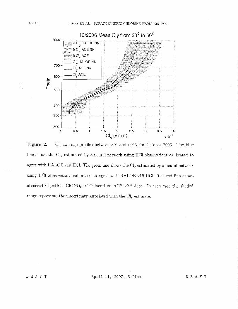
Figure 2 . C1, average profiles between 30" and 60°N for October 2006. The blue

line shows the C1, estimated by a neural network using HC1 observations calibrated to

agree with HALOE v19 HC1. The green line shows the C1, estimated by a neural network

using HCI observations calibrated to agree with HALOE v19 HC1. The red line shows

observed Cl,=HCl+C10N02+C10 based on ACE v2.2 data. In each case the shaded

range represents the uncertainty associated with the C1, estimate.

D R A F T A p r i l 11, 2007, 3:27pm D R A F T


4

3.5

3

2.5

1.5

1

0.5

0

Year

I995 ?.COO 2005 Year

, lo-vMonthly average 61° 4 . . . . . . . . . . . . . . . . . . c: r* ,I;<BW K

,

3.5 . . . . . . . . . . . .: . . . . . _"," ,r-.--. -_,- ---;~-i-'-* ----- :*-ii., qvTs 3. ---6YearAg

3 . .: g;~:;. .......... - - -5 YearAg --------?...-..--:--- ---4YearAg

2,5 , . . . . . . . . . . . . ---$Year& . . -2YearAg

-% . Lg.?:-~.=?2*--=:~-?c2<35. 0 -

1.5 ......................... ' ..... '........ j ....- : ,....

0.5 . . . . . . . . . . . . . . ,

1995 2000 2005 Year

Figure 3. Panels (a) to (c) show October C1, time-series for the 525 K isentropic

surface (E 20 km) and the 800 K isentropic surface (w 30 km). In each case a shaded

range representing the uncertainty in our estimate of C1, is shown. This uncertainty is

due to the biases between the various HC1 observations. The upper limit of the shaded

range corresponds to the estimate of C1, based on all the HCI observations calibrated

by a neural network to agree with ACE v2.2 HC1. The lower limit of the shaded range

corresponds to the estimate of C1, based on all the HC1 observations calibrated to agree

with HALOE v19 HC1. Overlaid are lines showing the C1, based on age of air calculations

[Newman et al., 20061. To minimize variations due to differing data coverage Months

with less than 100 observations of HC1 in the equivalent latitude bin were left out of the

time-series.


variations in stratospheric inorganic chlorine between ... · variations in stratospheric inorganic...

Documents