validated interactive daylighting analysis for ... · validated interactive daylighting analysis...

Validated Interactive Daylighting Analysis

for Architectural Design

by

Nathaniel Louis Jones

Bachelor of Science in Civil Engineering

Johns Hopkins University, 2005

Master of Architecture

Cornell University, 2009

Submitted to the Department of Architecture

in partial fulfillment of the requirements for the degree of

Doctor of Philosophy in Architecture: Building Technology

at the

Massachusetts Institute of Technology

June 2017

© 2017 Massachusetts Institute of Technology.

All rights reserved.

Signature of Author: ___________________________________________________________________

Department of Architecture

May 5, 2017

Certified by: ___________________________________________________________________

Christoph F. Reinhart

Associate Professor of Building Technology

Thesis Supervisor

Accepted by: ___________________________________________________________________

Sheila Kennedy

Chair, Departmental Committee on Graduate Students

3

Thesis Committee

Christoph F. Reinhart

Associate Professor of Building Technology


Thesis Supervisor

Frédo Durand

Professor of Electrical Engineering and Computer Science


Thesis Reader

Mehlika N. Inanici

Associate Professor of Architecture

University of Washington

Thesis Reader

5

Validated Interactive Daylighting Analysis

for Architectural Design

by

Nathaniel Louis Jones

Submitted to the Department of Architecture

on May 5, 2017 in partial fulfillment of the requirements

for the degree of Doctor of Philosophy in Architecture: Building Technology

Abstract

The conventional approach to predicting interior illumination and visual discomfort in buildings is to run a

ray tracing simulation with high accuracy settings, wait while the simulation processes, and repeat as

necessary with modifications to the scene and settings. This workflow lacks interactivity and usually occurs

late in the design process to validate a completed design, if at all. For architecture to benefit from daylight

as a practical, glare-free alternative to electric lighting, daylighting simulation and visual discomfort

predictions must be available in real time during design. This thesis describes three innovations towards

this goal: development of a parallel ray-tracing engine, validation against high dynamic range (HDR)

photography and annual simulations, and human subject tests with interactive progressive rendering.

Lighting simulation can be sped up more than an order of magnitude by running it in parallel on readily

available graphics processing units (GPUs). Accelerad is a GPU-accelerated version of RADIANCE synthetic

imaging software for global illumination simulation developed by the author, introducing a novel method

for parallel multiple-bounce irradiance caching. In validation studies comparing simulated and measured

luminance and visual discomfort, Accelerad achieves similar accuracy to RADIANCE at a speedup of 16 to

44 times. Applied to annual simulation methods to calculate climate based daylighting metrics such as

daylight autonomy and annual sun exposure, Accelerad is 10 times faster than DAYSIM and 25 times faster

than the five-phase method. Additionally, a progressive path tracing option is explored that calculates glare

probability in seconds and enables interactive visual discomfort simulation.

By providing accurate lighting simulation results to designers in real time, this information is expected to

inform the design process in ways not previously possible. In human subject tests, the availability of real-

time feedback was associated with increased exploration of the design space, higher confidence in proposed

designs, higher satisfaction with the design task, and better performing designs with respect to daylight

autonomy and daylight glare probability. This supports the theory that system response time affects users’

cognitive states and suggests that designers will be more likely to adopt building performance simulation

tools if they produce reliable results at interactive speeds.

Thesis Supervisor: Christoph F. Reinhart

Title: Associate Professor of Building Technology

7

Acknowledgments

I owe much to my advisor, Professor Christoph Reinhart, for his constant interest and support for my work.

I have known Christoph since 2010 when I was just starting to work on GPU-accelerated building

performance simulation, and the idea to parallelize RADIANCE for GPU computation is his brainchild. Over

the last four years, Christoph has helped and challenged me to push my research forward. Most importantly,

he has shown a keen interest when my research veered outside the confines of architecture and his own

expertise, and in doing so he has shown me how to become a better researcher and communicator.

I extend my gratitude to the members of my thesis committee. Professor Frédo Durand’s technical insight

in computer graphics and GPU programming has been invaluable, and his editorial guidance was

indispensable to my work on irradiance caching. Professor Mehlika Inanici’s experience with HDR

photography and sky observation made the validation efforts in this thesis possible.

This thesis would not have been possible without RADIANCE, which Greg Ward has developed for the last

thirty years. Greg has been constantly available to answer questions and provide feedback, and he has

shown an incredible willingness to support Accelerad with minor changes in the RADIANCE source code.

Rob Guglielmetti’s upkeep of the RADIANCE mirror repository on GitHub has also been vital on more than

one occasion.

I have benefitted from the wisdom and research of many students who have preceded me in the Sustainable

Design Lab. Alstan Jakubiec contributed models that I continue to use in Accelerad tests, as well as help in

accurate modeling of material reflectance. Jon Sargent developed the Grasshopper components that allowed

interactivity between Rhinoceros and Accelerad. Timur Dogan and Manos Saratsis inspired my interest in

annual simulation and ran early tests of it.

Many people at MIT played a role in the physical testing and user studies that I carried out. Professor Les

Norford and Jim Harrington provided the roof access that made the validation study possible, and Matt

Aldrich and Susanne Seitinger supported my early validation work in the Media Lab. Philip Thompson

provided necessary technical support for the user study, and I thank Les again for the use of his office to

carry out the study.

Personal correspondence and meetings with many other researchers have aided my research. Jaroslav

Křivánek offered useful insight into previous work on irradiance caching. Frédo’s students Tzu-Mao Li,

Shuang Zhao, and Lukas Murmann have all contributed insight into rendering and ray tracing. Andy McNeil

and Eleonora Brembilla provided helpful background to implementing and validating the three- and five-

phase methods. John Mardaljevic contributed to my understanding of the useful daylight illuminance

metric.

MIT’s building technology program and the Sustainable Design Lab have been a second home for me for

the last four years. My thanks go to my fellows in this community: Aiko, Ali, Alonso, Alpha, Alstan, Amir,

André, Arfa, Brad, Carlos, Catherine, Cody, David, Irmak, Jamie B., Jamie F., Jay, Jeff, Jonathan, Julia,

Khadija, Leo, Lidia, Liz, Lup Wai, Madeline, Nathan, Nelson, Noor, Nourhan, Pierre, Qin, Renaud,

Richard, and Tarek. Thanks to Ammar Ahmed for his help and for the exploded figure of a computer

monitor. Above all, thank you to Kathleen Ross for the smooth operation of our lab.

8

Portions of my research were funded through the Kuwait-MIT Center for Natural Resources and the

Environment by the Kuwait Foundation for the Advancement of Sciences. The Tesla K40 accelerators used

for this research were donated by the NVIDIA Corporation.

I am thankful to my former advisor Professor Kevin Pratt for inspiring my interest in building science.

Together with Professors Don Greenberg, Ken Torrance, and Brandon Hencey at Cornell University, he

started me on my path to research in building technology.

Finally, thank you to my wife, Robin. In the time we have known each other, she has been my strongest

supporter, and in her proofreading, she has been my harshest critic. I look forward to the next stage of our

adventure together.

9

In almost every computation a great variety of arrangements for the succession of the processes is possible,

and various considerations must influence the selections amongst them for the purposes of a calculating

engine. One essential object is to choose that arrangement which shall tend to reduce to a minimum the

time necessary for completing the calculation.

—Ada Lovelace

Essentially, all models are wrong, but some are useful.

—George Box

IN MEMORIAM

Kevin Pratt

13

Table of Contents

1 Introduction ......................................................................................................................................... 17 1.1 RADIANCE and Accelerad ........................................................................................................... 18 1.2 Dissertation Overview................................................................................................................. 19

2 Literature Review ................................................................................................................................ 23 2.1 Speed ........................................................................................................................................... 23

2.1.1 System Response Time ....................................................................................................... 23 2.1.2 Moore’s Law ....................................................................................................................... 24 2.1.3 Parallel Computing ............................................................................................................. 25 2.1.4 Simulation and Ray Tracing on the GPU ............................................................................ 25

2.2 Accuracy ..................................................................................................................................... 26 2.2.1 Measuring Daylight............................................................................................................. 26 2.2.2 Visual Discomfort ............................................................................................................... 27 2.2.3 Validation Studies ............................................................................................................... 28

3 Fundamentals of Accelerad ................................................................................................................. 31 3.1 Design Decisions ........................................................................................................................ 31

3.1.1 Data Preparation .................................................................................................................. 31 3.1.2 Shaders ................................................................................................................................ 32 3.1.3 Command-Line Arguments ................................................................................................. 33

3.2 Tests Comparing RADIANCE and Accelerad ............................................................................... 34 3.2.1 rpict ..................................................................................................................................... 34 3.2.2 rtrace ................................................................................................................................... 36

3.3 Initial Accomplishments and Shortcomings ............................................................................... 37

4 Irradiance Caching .............................................................................................................................. 39 4.1 How It Works .............................................................................................................................. 39

4.1.1 Serial Irradiance Caching .................................................................................................... 40 4.1.2 Parallel Irradiance Caching ................................................................................................. 40

4.2 Fixed-Sized Caching Algorithms ................................................................................................ 41 4.2.1 Reading from an Irradiance Cache in Parallel .................................................................... 41 4.2.2 Creating an Irradiance Cache for Enclosed Spaces ............................................................. 42 4.2.3 Creating an Irradiance Cache for Open Spaces ................................................................... 44

4.3 Validation of the Fixed-Sized Irradiance Cache ......................................................................... 45 4.3.1 Enclosed Space ................................................................................................................... 46 4.3.2 Open Space ......................................................................................................................... 47

4.4 The Problem of Coverage ........................................................................................................... 48 4.5 Dynamically-Sized Caching Algorithms .................................................................................... 49

4.5.1 Coarse Geometry Sampling ................................................................................................ 50 4.5.2 Coarse Irradiance Sampling ................................................................................................ 52 4.5.3 Fine Geometry Sampling .................................................................................................... 52 4.5.4 Fine Irradiance Sampling .................................................................................................... 52

14

4.6 Validation of the Dynamically-Sized Irradiance Cache .............................................................. 53 4.6.1 Illumination Sources ........................................................................................................... 53 4.6.2 Comparison Metrics ............................................................................................................ 54

4.7 Speed and Accuracy .................................................................................................................... 55 4.8 Summary ..................................................................................................................................... 58

5 Validation Studies ............................................................................................................................... 61 5.1 Sky Luminance ........................................................................................................................... 61 5.2 Preliminary Study ....................................................................................................................... 61

5.2.1 Simulation Accuracy ........................................................................................................... 63 5.2.2 Error Sources ...................................................................................................................... 64

5.3 An Improved Validation Method ................................................................................................ 65 5.4 Data Acquisition ......................................................................................................................... 67

5.4.1 Cameras ............................................................................................................................... 68 5.4.2 Light Sources ...................................................................................................................... 69 5.4.3 Geometry and Materials ...................................................................................................... 73 5.4.4 Display Monitor .................................................................................................................. 73

5.5 Simulations ................................................................................................................................. 75 5.5.1 Comparison Metrics ............................................................................................................ 75 5.5.2 Computing Environment ..................................................................................................... 76

5.6 Sensitivity Analysis .................................................................................................................... 76 5.7 Accuracy Analysis ...................................................................................................................... 77

5.7.1 Pixel-Level Error................................................................................................................. 80 5.7.2 Photometric Error ................................................................................................................ 80 5.7.3 Daylight Glare Probability and Local Contrast ................................................................... 83

5.8 Speed Analysis ............................................................................................................................ 86 5.9 Recommendations ....................................................................................................................... 87

5.9.1 Choosing a Sky ................................................................................................................... 88 5.9.2 Choosing Simulation Parameters ........................................................................................ 89 5.9.3 Choosing Simulation Tools ................................................................................................. 90

5.10 Summary ..................................................................................................................................... 90

6 Annual Simulation .............................................................................................................................. 91 6.1 Calculating Climate-Based Daylighting Metrics ........................................................................ 91

6.1.1 DAYSIM ............................................................................................................................. 92 6.1.2 Three- and Five-Phase Methods.......................................................................................... 92 6.1.3 Validation ............................................................................................................................ 93

6.2 Implementation ........................................................................................................................... 93 6.2.1 Ray Payloads ....................................................................................................................... 94 6.2.2 Global Memory Use ............................................................................................................ 95

6.3 Performance Comparison ............................................................................................................ 96 6.3.1 Daylight Metrics ................................................................................................................. 98 6.3.2 Speedup ............................................................................................................................... 99

6.4 Needs and Recommendations ................................................................................................... 102

15

7 Real-Time Glare Analysis ................................................................................................................. 105 7.1 Progressive Path Tracing .......................................................................................................... 105 7.2 Prototype Tests .......................................................................................................................... 106

7.2.1 Image Quality .................................................................................................................... 107 7.2.2 Vertical Eye Illuminance .................................................................................................. 108 7.2.3 Daylight Glare Probability ................................................................................................ 109 7.2.4 Task Area Luminance and Contrast Ratio ........................................................................ 110

7.3 Experiment Setup ...................................................................................................................... 112 7.3.1 Design Task ...................................................................................................................... 112 7.3.2 Tool Design ....................................................................................................................... 115

7.4 User Study Results .................................................................................................................... 116 7.4.1 User Behaviors and Design Strategies .............................................................................. 116 7.4.2 Design Performance .......................................................................................................... 121 7.4.3 User Evaluations ............................................................................................................... 125

7.5 Recommendations ..................................................................................................................... 127 7.5.1 Recommendations for Tools ............................................................................................. 127 7.5.2 Recommendations for Metrics .......................................................................................... 128

7.6 Summary ................................................................................................................................... 129

8 Conclusions and Outlook .................................................................................................................. 131 8.1 A Grain of Salt .......................................................................................................................... 131 8.2 Interactive Performance-Based Design ..................................................................................... 132 8.3 Immersive Environments .......................................................................................................... 133 8.4 Visual Comfort Metrics ............................................................................................................ 135 8.5 Where Are the Limits? .............................................................................................................. 136

References ................................................................................................................................................. 139

List of Abbreviations ................................................................................................................................ 153

1 Introduction

Why make things go fast? An equivalency between “faster” and “better” pervades our culture, from work

and technology to sports and entertainment [1]. Design professionals might reason based on their experience

with currently available tools that quick calculations are necessarily less accurate or less trustworthy than

longer-running simulations. We1 argue that increased computational speed does directly benefit

designers, and that a tradeoff between speed and accuracy is avoidable. In this thesis, we advance two

hypotheses. First, parallel computing can make simulations more than an order of magnitude faster

without loss of accuracy. Second, tools designed for speed will foster interactive design processes that

can produce a more sustainable built environment.

This is a thesis on daylighting, which we define as the use of natural light to provide sufficient and

comfortable illumination in buildings. However, our research is equally relevant to other design fields and

to other areas of building performance simulation, which allow users to predict, plan, and manage resources

in the built environment. We focus on daylighting simulation because it is conceptually simple and has the

potential for large speedups when ported to run on graphics processing units (GPUs). In programming

parlance, daylighting simulation is embarrassingly parallel, meaning that we can easily break each

simulation into many independent calculations for simultaneous execution. Daylighting thus allows us to

indulge our main interest: How to make simulation results available to designers at interactive speeds so

that validated performance predictions can most effectively influence design decisions.

Architects and lighting designers use software tools to predict light levels to achieve qualitative design

goals and to meet quantitative illumination requirements. Increasingly, illumination goals focus on the

aesthetic [2] and functional role of daylight [3, 4], which are highly time-dependent and in which indirect

lighting plays a major role. To these ends, the design community depends on predictive rendering and

climate-based daylighting metrics. Predictive rendering refers to image synthesis whose goal is not to look

plausible but rather to verifiably match the physical scene once built. High dynamic range (HDR) images

created by physically based predictive rendering can accurately predict luminance values experienced by

the human eye and predict occurrence of visual discomfort. Climate-based daylighting metrics (CBDMs)

represent the annual daylighting performance of a space affected by local weather. CBDMs are abstract

quantities that aggregate data across space and time, but they can agree closely with concrete occupant

observations [5].

Unfortunately, predictive rendering and CBDM simulation tools currently available to the design

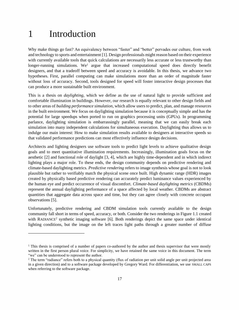
community fall short in terms of speed, accuracy, or both. Consider the two renderings in Figure 1.1 created

with RADIANCE2 synthetic imaging software [6]. Both renderings depict the same space under identical

lighting conditions, but the image on the left traces light paths through a greater number of diffuse

1 This thesis is comprised of a number of papers co-authored by the author and thesis supervisor that were mostly

written in the first person plural voice. For simplicity, we have retained the same voice in this document. The term

“we” can be understood to represent the author. 2 The term “radiance” refers both to a physical quantity (flux of radiation per unit solid angle per unit projected area

in a given direction) and to a software package developed by Gregory Ward. For differentiation, we use SMALL CAPS

when referring to the software package.

17

18

reflections. Consequently, it both depicts more accurate interior luminance levels and takes roughly thirty

times longer to compute. What would happen if an architect wanted to redesign the space based on one of

these simulations? Choosing the simulation that created the image on the right would leave the designer

misinformed about the luminous environment of the space and might lead to a redesign with larger windows

that could expose occupants to solar overheating and glare. Conversely, choosing longer running simulation

would distract the architect from the task for nearly an hour. This dilemma will lead many designers to

abandon the use of simulations altogether or until later in the design process when a concept has matured

and less flexibility for change remains.

49 minutes 1.5 minutes

138,844,405 rays 41,010,721 rays

102 103 104 cd/m2

Figure 1.1 The accurate RADIANCE rendering (left) takes too much time to use in interactive

design, while the fast rendering (right) is misleading.

This thesis describes work on Accelerad, a new software package that duplicates the ray tracing

functionality of RADIANCE on a GPU. Using parallel processing on the GPU, we hope to overcome the

perceived tradeoff between speed and accuracy. Accelerad has two primary objectives: To produce

physically based lighting simulation results with at least the accuracy of RADIANCE, and to do so fast

enough to facilitate informed, interactive designing.

1.1 RADIANCE and Accelerad

RADIANCE has become a staple of the architectural and lighting design communities due to its widespread

adoption and well-validated results [7]. RADIANCE is a collection of software programs, not an application,

and the RADIANCE ecosystem includes three types of programs. These are the core RADIANCE programs,

various derivative works, and a variety of graphic user interfaces that call on RADIANCE and its derivatives.

19

The core RADIANCE programs use light-backward distribution ray tracing, in which primary rays originate

from a point (a virtual camera or illuminance sensor) to sample the environment. Wherever a ray intersects

a surface, it recursively spawns one or more new rays, depending on the surface material, and gathers their

results into a single value that is returned as the parent ray’s result [8]. Typically, a small number of spawned

rays are required for direct and specular reflections, and a much larger number of rays spawn to sample the

indirect irradiance due to ambient lighting at the intersection point. Consequently, ambient calculations tend

to dominate the total ray tracing computation time. In RADIANCE, each ray returns red, green, and blue

(RGB) values in units of radiance (W·sr-1·m-2). The array of values returned from the primary rays produces

an image or a grid of sensor values.

The second class of tools are derivative works based on RADIANCE that alter its source code in order to add

new functionality. For example, DAYSIM is a modification of RADIANCE that calculates daylight

coefficients instead of red, green, and blue channels for each ray [9]. Accelerad belongs to this second class

of programs. To create Accelerad, we modified the RADIANCE source code to call the OptiX™ GPU ray-

tracing library created by NVIDIA® [10]. In this thesis, we discuss modified versions of five RADIANCE

programs that together comprise Accelerad:

rtrace simulates radiance or irradiance at individual sensors. These sensors may form a grid over a

work plane, or they may represent individual view directions for pixels of an image.

rpict renders images, mimicking a high-dynamic range camera (which is a closely-packed array of

directional sensors).

rcontrib calculates the radiant contributions of sources and surfaces to sensor points. It facilitates

dynamic daylight simulations based on a single ray-tracing pass.

rvu provides limited interactive model visualizations for debugging purposes.

rtrace-dc calculates daylight coefficients and is part of DAYSIM. It is itself a derivative of rtrace.

The third class of tools are user interfaces to RADIANCE and its derivatives. These include widely used

building performance simulation tools such as IES<VE>, Ecotect®, OpenStudio, Honeybee, and DIVA-for-

Rhino. These tools access RADIANCE and DAYSIM through a UNIX-style command-line interface and use

it as a simulation engine for daylighting and electric lighting simulations. Users may not even be aware of

RADIANCE running as a separate process. We designed Accelerad to accept the same command-line prompts

so that these user interfaces can call it and the original RADIANCE and DAYSIM programs interchangeably.

1.2 Dissertation Overview

This thesis combines a number of studies that report the development and validation of Accelerad and

related algorithms. Most of these studies have been published or are in the process of being published. Their

ordering in this document is thematic rather than chronologic; we start with the topics most fundamental to

Accelerad and proceed to validations of visual comfort and CBDM simulation and extensions into real-

time simulation.

Although all of these chapters deal with Accelerad, the Accelerad code based grew and evolved

significantly over the course of this investigation. Perhaps more importantly, many of these chapters deal

20

with specific Accelerad programs and use different algorithms for calculating the diffuse component of

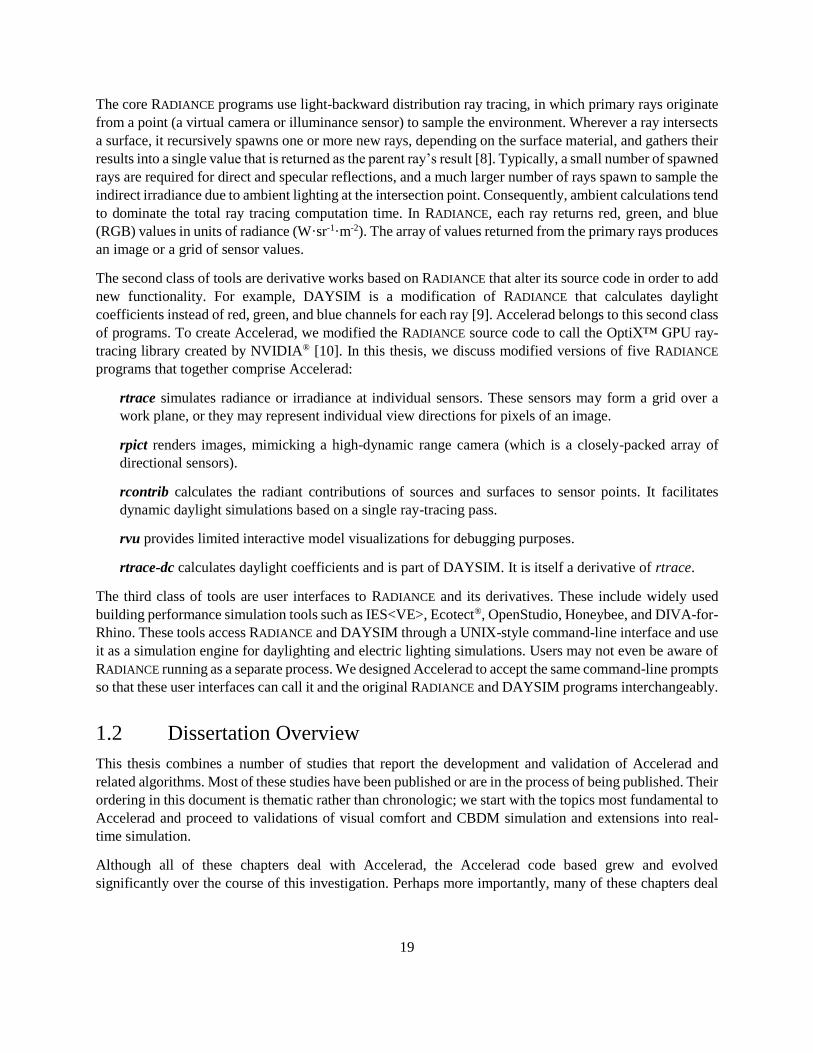
global illumination. Figure 1.2 summarizes the chapters in which each program and algorithm appear.

CHAPTER

3 4 5 6 7

PROGRAM

rtrace

rpict

rcontrib

rvu

rtrace_dc

ALGORITHM

Distribution ray tracing

with fixed-size irradiance cache

with dynamic irradiance cache

with Russian roulette

Progressive path tracing

Figure 1.2 A guide to the appearance of Accelerad programs and global illumination

algorithms by chapter.

Chapters 1 and 2 introduce Accelerad and explain the need for a fast and accurate daylighting design tool.

Chapter 2 contains background research on the speed and accuracy of RADIANCE tools. We use this

background information to formulate two research goals. First, we set a goal for simulation speed based on

studies of user interaction and explain why achieving this speed requires parallelism. Second, we set a goal

for simulation accuracy based on previous validation studies and describe the metrics that we will use in

this thesis to quantify lighting and visual discomfort.

Chapter 3 examines the feasibility of implementing core algorithms from RADIANCE in parallel in a GPU

environment [11]. It presents solutions to a number of implementation challenges, including how to

reinterpret the RADIANCE data format as a set of GPU-compatible buffered data arrays, how to break up the

ray-tracing core of the RADIANCE programs into a number of small GPU programs that execute in parallel,

and how to apply settings chosen by the user on the GPU. These design decisions are simple but important

because they affect how we implement other improvements in later chapters. We developed Accelerad as

a proof of concept for this study and show that it produces images indistinguishable from RADIANCE up to

twenty times faster simply using parallelism in the absence of irradiance caching.

Chapter 4 describes a novel method of parallel multiple-bounce irradiance caching on a GPU that further

speeds up simulations. Irradiance caching is difficult to parallelize because efficient solutions depend on

the order in which calculations occur. The chapter presents results from two investigations [12, 13]. The

first study describes how we create an irradiance cache of fixed size in parallel. In the second study, we

allow the cache size to vary dynamically. We show by comparison to HDR photography of a moderately

complex space that our method can predict luminance distribution as accurately as RADIANCE does with

irradiance caching, and that it is faster by an order of magnitude.

Chapter 5 presents work we have done to validate the accuracy of Accelerad simulations. We compare

simulation results from RADIANCE and Accelerad with measurements from calibrated HDR photographs.

21

We use vertical eye illuminance, daylight glare probability, and monitor contrast ratio as metrics for

comparison. The chapter presents the results of two studies [14, 15] that compare the accuracy of RADIANCE

and Accelerad in naturally lit environments. The first study reveals issues arising from inaccurate

representation of the sky’s luminance distribution. The second study improved sky modeling and image

capture to predict daylight glare probability levels due to bright sources with between 93% and 99%

accuracy and discomfort glare due to contrast with between 71% and 99% accuracy. Using Accelerad, we

achieve a speedup over RADIANCE of between 16 and 44 times.

In Chapter 6, we turn our attention from predictive rendering to CBDM simulation. The chapter presents

the work from two studies [16, 17]. The first study describes Accelerad’s parallelization of DAYSIM’s

rtrace_dc [9]. In the second study, we parallelize the rcontrib algorithm used in the three-phase method

[18] and the five-phase method [19] for CBDM calculations. Using a model of a generic office, we achieve

speedups of ten times with DAYSIM and twenty-five times with the five-phase method.

In Chapter 7, we break from RADIANCE’s ray tracing algorithm to investigate an alternative method,

progressive path tracing, which produces results in real time. The chapter presents the results of two studies.

The first study [20] shows that progressive path tracing can produce live-updating predictions of daylight

glare probability, task luminance, and contrast alongside a progressively rendered image of the scene. In

most cases, sufficiently accurate results are available within seconds after rendering only a few frames. In

the second, a human subjects study, forty subjects with backgrounds in building design and technology

carried out two shading design exercises to balance glare reduction and annual daylight availability in two

open office arrangements using two simulation tools with differing system response times. Subjects with

access to real-time simulation feedback tested more design options, reported higher confidence in design

quality and increased satisfaction with the design task, and produced better-performing final designs

regarding daylight autonomy and daylight glare probability.

Finally, Chapter 8 presents conclusions and an outlook for the field. We predict that the availability of fast

and accurate simulation will lead architects to use performance-based design workflows and suggest

immersive environments as a novel and useful application of our work. We also discuss the need for new

performance metrics and new ways of interacting with simulation feedback such as through virtual reality.

We conclude with a discussion of the limits of simulation speed and accuracy.

23

2 Literature Review

Software tools have changed the nature of design thinking significantly in the last half-century. Computer-

aided design (CAD) emphasizes specificity and detail over abstract representation [21], and designers

exhibit different design strategies when using CAD tools than when sketching, according to think-aloud

design studies [22]. The choice of simulation tool may produce different performance results [23] and elicit

different user behavior [24]. We use this literature review to set goals for the speed and accuracy of

simulation software generally, and Accelerad in particular, to be most useful to designers.

2.1 Speed

We know that simulations should be fast in order to aid in design, but how fast is enough? In this section,

we lay out previous research to show that the response time of a computer system has a cognitive effect on

its user, and we define a range of response times that may be considered interactive. We then examine the

progress of hardware manufacturers and conclude that GPU parallelism is necessary to make RADIANCE

interactive. Finally, we describe previous work in parallelizing building performance simulation tools using

GPUs. We set a goal for simulation speed based on our understanding of interactive response times.

2.1.1 System Response Time

In order for simulation results to inform design decisions, they must be available as the designer makes

those decisions. We are referring to decisions made during active designing, not those made in the

boardroom after the fact, so informed decisions require interactivity. System response time (SRT) is the

time a user waits after entering input before the system begins to present results to the user [25]. Studies

conducted at IBM show that SRT affects productivity, but not simply by adding SRT to the time required

for task completion. Instead, longer SRT seems to “disrupt the thought process” and cause a longer user

response time as well [25]. A pause as short as two seconds may cause disruption, but reducing SRT

increases productivity, job satisfaction, design quality, and perceived power, and decreases anxiety levels

[26, 27, 28, 29]. From these observations, Brady developed roll theory, which states that given immediate

access to organized data and with concentration unbroken by distractions, “ideas and solutions will suggest

more ideas and solutions to successive steps of the creative process, in a rapid and orderly flow” [30]. When

“on a roll,” an average user can exhibit higher productivity than an expert user faced with high SRT [26].

Brady’s theory seems intrinsically related to Csíkszentmihályi’s concept of flow [31]. Flow is a focused

mental state in which tasks seem effortless, which Csíkszentmihályi characterizes with nine traits:

1. Clear goals at every step

2. Immediate feedback to one’s actions

3. Balance between challenges and skills

4. Actions and awareness are merged

5. Distractions are excluded from consciousness

6. No worry of failure

7. Self-consciousness disappears

8. Sense of time becomes distorted

9. Activity becomes autotelic

24

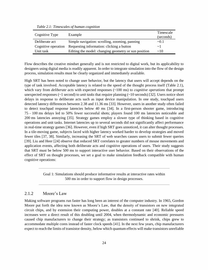
Table 2.1: Timescales of human cognition

Cognitive Type Example Timescale

(seconds)

Deliberate act Simple navigation: scrolling, zooming, panning ~0.1

Cognitive operation Requesting information: clicking a button ~1

Unit task Editing the model: changing geometry or sun position ~10

Flow describes the creative mindset generally and is not restricted to digital work, but its applicability to

designers using digital media is readily apparent. In order to integrate simulation into the flow of the design

process, simulation results must be clearly organized and immediately available.

High SRT has been noted to change user behavior, but the latency that users will accept depends on the

type of task involved. Acceptable latency is related to the speed of the thought process itself (Table 2.1),

which vary from deliberate acts with expected responses (~100 ms) to cognitive operations that prompt

unexpected responses (~1 second) to unit tasks that require planning (~10 seconds) [32]. Users notice short

delays in response to deliberate acts such as input device manipulation. In one study, touchpad users

detected latency differences between 2.38 and 11.36 ms [33]. However, users in another study often failed

to detect touchpad response latencies below 40 ms [34]. In a first-person shooter game, introducing

75 – 100 ms delays led to 50% fewer successful shots; players found 100 ms latencies noticeable and

200 ms latencies annoying [35]. Strategy games employ a slower type of thinking based in cognitive

operations and unit tasks. Internet latencies up to several seconds did not significantly affect performance

in real-time strategy games [36]. However, even if high SRT goes unnoticed, it can alter thought processes.

In a tile-moving game, subjects faced with higher latency worked harder to develop strategies and moved

fewer tiles [37, 38]. Similarly, increasing the SRT of web searches causes users to submit fewer queries

[39]. Liu and Heer [24] observe that reduced SRT correlates to greater numbers of mouse movements and

application events, affecting both deliberate acts and cognitive operations of users. Their study suggests

that SRT must be below 500 ms to support interactive user behavior. Based on their observations of the

effect of SRT on thought processes, we set a goal to make simulation feedback compatible with human

cognitive operations:

Goal 1: Simulations should produce informative results at interactive rates within

500 ms in order to support flow in design processes.

2.1.2 Moore’s Law

Making software programs run faster has long been an interest of the computer industry. In 1965, Gordon

Moore put forth the idea now known as Moore’s Law, that the density of transistors on new integrated

circuit chips, and by extension their computing power, doubles at a constant rate [40]. Reliable speed

increases were a direct result of this doubling until 2004, when thermodynamic and economic pressures

caused chip manufacturers to change their strategy; as transistors continued to shrink, chips grew to

accommodate multiple cores instead of faster clock speeds [41]. In the next few years, chip manufacturers

expect to reach the limits of transistor density, below which quantum effects will make transistors unreliable

25

[42]. In this post-Moore era, continued software speedups need to come from parallelism and compiler

optimization [43].

Moore’s Law gave simulation tools like RADIANCE a free ride for many years. As long as central processing

unit (CPU) clock speeds dependably doubled every 1.5 to 2 years in accordance with the law, users could

pursue ever more complicated simulations with assurance that the calculations would speed up accordingly

on new generations of hardware. A 2005 estimate proposed that ray tracing speeds must increase by two

orders of magnitude over CPU speeds in order to achieve interactive performance [44]. However, we can

no longer depend on innovations in hardware to speed up serial computation. Without steadily increasing

processor speeds, we must use parallelism to achieve that goal. We turn our attention to GPUs because they

offer the potential for massive parallelism on commodity hardware.

2.1.3 Parallel Computing

Like many contemporaneous simulation programs, RADIANCE performs calculations in serial; it runs in a

single thread that carries out its programmatic instructions in sequential order. In contrast, a program that

runs in parallel uses two or more threads to execute different chains of instructions simultaneously. Each

thread executes on a physical processor, or core. The terms thread and core are often used interchangeably,

though they are not synonymous (multiple threads may execute on the same core at different times, and

some cores may go unused). When a serial program is rewritten to execute in parallel, the theoretical

speedup is limited by the number of available cores and the fraction of the program that cannot be

parallelized [45]. This relationship is known as Amdahl’s Law [46].

While CPU cores essentially act independently of each other, the design of GPUs sacrifices core

independence for quantity. A warp is a group of 32 threads that execute simultaneously on one of the GPU’s

multiprocessors [47]. This computer architecture is generally well suited to vector and matrix computations

using a single-instruction, multiple-data (SIMD) programming model in which the same operation is

applied simultaneously to each thread in the warp. SIMD architecture makes large speedups possible

through parallelism.

Ray tracing is highly parallel in concept because each primary ray acts independently of other rays and can

be assigned to a separate thread. However, if rays in the same warp intersect surfaces with different

materials, the threads may need to execute divergent instructions. Rather than SIMD, this necessitates a

single-instruction, multiple-thread (SIMT) architecture where the multiprocessor can execute different

instructions for different threads within the warp. Divergent behavior introduces programmatic

inefficiencies because not all threads in the warp may be active at any given time [47].

2.1.4 Simulation and Ray Tracing on the GPU

The high degree of parallelism built into modern GPUs makes their use appealing for scientific applications.

In building performance simulation, they have been used mainly for computations involving manipulation

of dense matrices, including applications in computational fluid dynamics [48, 49], acoustics [50, 51, 52],

and incident solar radiation [53, 54, 55]. Zuo et al. [56] implemented the matrix multiplication portion of

the three-phase method in parallel on GPUs, achieving a speedup of 800 times over previous methods for

that step, but did not parallelize the ray tracing operations that account for most of the simulation time.

Jones, et al., [53] reduced direct solar radiation calculations to a manipulation of dense matrices in

OpenGL®, and Kramer, et al., [55] extended this solution to general direct radiant heat exchange.

26

Early GPU ray tracers relied significantly on coopting elements of the raster pipeline and imitated its state

machine programming interface [57, 58]. GPU language extensions such as Compute Unified Device

Architecture (CUDA®) from NVIDIA® [47] and OpenCL™ from the Khronos™ Group make it possible

to implement ray tracing on GPU shader processors [59]. Introducing a second layer of parallelism, large

data processing jobs may be partitioned and distributed among multiple GPUs [60]. In computational

physics, multi-GPU environments can yield significant speedups [61, 62, 63].

In 2010, NVIDIA® released the OptiX™ ray tracing engine, which uses CUDA® to perform both ray

traversal and shading on the GPU [10]. The OptiX™ library is designed to replace serial CPU-based ray

tracing engines in existing source code. OptiX™ provides built-in acceleration structure creation and ray

traversal algorithms to detect potential ray-surface intersections. The programmer is only required to re-

implement ray generation, intersection testing, closest hit, any hit, and miss algorithms as CUDA®

programs. OptiX™ compiles these programs into assembly code and uses a just-in-time compiler to create

device-specific instructions at runtime. OptiX™ has been used to accelerate other building performance

simulation tasks. Clark [64] and Halverson [65] demonstrate its use for modeling radiative heat transfer

involved in the urban heat island effect. Andersen et al. [66] use it for interactive visualization of cached

RADIANCE results. Currently, there is no well-supported OpenCL™ alternative to OptiX™, although recent

work from Intel® now provides an optimized CPU-based alternative [67, 68].

2.2 Accuracy

Using GPU parallelism, we can speed up RADIANCE simulations without necessarily changing their

accuracy. In this section, we report on previous research about the accuracy we can expect from lighting

metrics. First, we present a number of metrics that quantify lighting sufficiency and visual discomfort.

Then, we examine validation studies that have been carried out against either photographic or sensor-based

references and form a goal for accuracy from their consensus.

2.2.1 Measuring Daylight

The amount of daylight present in a building at any given time depends on the sun’s position and current

weather conditions. Historically, lighting standards have focused on meeting minimum illuminance

requirements for tasks. Growing interest in reducing energy demand through the use of natural light,

combined with advances in annual lighting simulation, led to the development of climate-based daylighting

metrics (CBDMs) such as spatial daylight autonomy and annual sunlight exposure that describe daylighting

over a space’s annual occupied hours [3]. These metrics are now integrated into compliance paths for both

the LEED [69] and WELL [70] green building standards. Spatial daylight autonomy describes the fraction

of occupied space that receives at least 300 lux for at least 50% of occupied hours and is abbreviated

sDA300,50%. Annual sunlight exposure is the fraction of occupied space that receives at least 1000 lux (and

can therefore be assumed to be in direct sunlight) during at least 250 occupied hours and is abbreviated

ASE1000,250. Designers should attempt to maximize sDA300,50% and minimize ASE1000,250 to provide adequate

natural illumination without overheating [3].

Recently, interest among researchers and practitioners has expanded from illuminance to luminance-based

analysis, which measures light incident on the eye and is more directly involved in human perception and

therefore visual comfort. Luminance simulation may predict the sense of stimulation and excitement

experienced by building occupants [2] as well as circadian response to buildings [71, 4].

27

2.2.2 Visual Discomfort

Glare is a subjective human phenomenon in which vision is impaired or strained due to unfavorable

luminance levels within a person’s field of view. Indoor glare may be classified into three types. Disability

glare occurs when a bright light source in the field of view measurably impairs vision, resulting in a loss of

contrast in the retinal image [72]. Discomfort glare causes visual irritation but not impairment; it may

become disability glare if the source is made larger or brighter [73]. Veiling glare occurs when the glare

source is seen indirectly through reflection; this phenomenon is experienced when light falling on a monitor

screen obscures the display [74]. In outdoors settings, glare is assessed by its potential to produce temporary

after-images or permanent eye damage [75].

2.2.2.1 Contrast Ratios

Contrast ratios provide a simple metric for quantifying glare. They compare the relative luminance values

of two regions in the field of view and may be measured using a luminance meter or by comparing values

in a calibrated high dynamic range (HDR) image. Veiling glare on a monitor is quantified by the contrast

ratio CRv:

𝐶𝑅𝑣 =𝐿𝐻 + 𝐿𝑟

𝐿𝐿 + 𝐿𝑟 (2.1)

where LH is the high state luminance of a bright pixel, LL is the low state luminance of a dark pixel, and Lr

is the luminance contribution from reflected light. In practice, we measure the numerator and denominator

sums of Equation (2.1) directly. Older standards require a minimum CRv of 3 [76] to preserve legibility.

More recent standards [77] vary the minimum acceptable ratio CRmin depending on low state luminance:

𝐶𝑅𝑚𝑖𝑛 = 2.2 + 4.84(𝐿𝐿 + 𝐿𝑟)−0.65 (2.2)

and may additionally modify CRmin to consider factors such as the age of the viewer. While Equation (2.2)

was derived from visual detection tasks involving a light target against a dark background [78], it is now

generally used as a standard for the inverse scenario.

Discomfort glare may occur when the brightness of a vertical or horizontal work surface differs significantly

from its surroundings. For example, direct sunlight falling on a work surface may cause the surface to

behave as a glare source. Discomfort glare due to work surface contrast is described by the contrast ratio

CRd:

𝐶𝑅𝑑 =𝐿𝑠

𝐿𝑡 (2.3)

where Lt is the task area luminance and Ls is the luminance of the surrounding region. We are not aware of

any human subject studies to recommend comfortable limits on CRd, but a popular rule of thumb for

artificially lit spaces is to maintain 1/3 < CRd < 3 for near-field surroundings and 1/10 < CRd < 10 for far-

field surroundings [79]. We consider only the 10:1 and 1:10 ratios in this manuscript.

2.2.2.2 Glare Indices

Glare indices quantify glare likelihood by examining the entire human field of vision. Typically, these

metrics rate glare sources based on size, position within the field of view, and brightness in relation to the

average background luminance. A number of metrics exist, including the Daylight Glare Index (DGI) [73],

28

CIE Glare Index (CGI) [80], Unified Glare Rating (UGR) [72], New Daylight Glare Index (DGIN) [81],

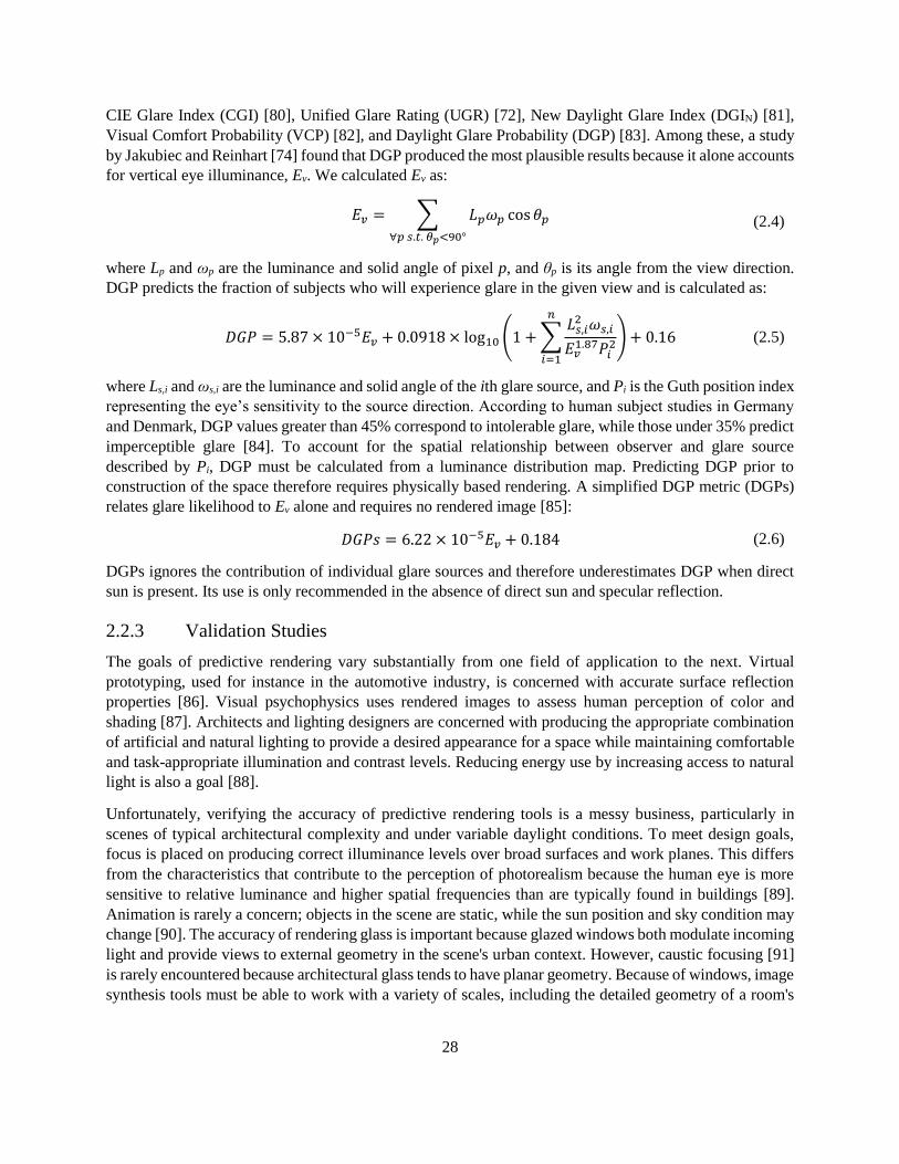
Visual Comfort Probability (VCP) [82], and Daylight Glare Probability (DGP) [83]. Among these, a study

by Jakubiec and Reinhart [74] found that DGP produced the most plausible results because it alone accounts

for vertical eye illuminance, Ev. We calculated Ev as:

𝐸𝑣 = ∑ 𝐿𝑝𝜔𝑝 cos 𝜃𝑝

∀𝑝 𝑠.𝑡. 𝜃𝑝<90°

(2.4)

where Lp and ωp are the luminance and solid angle of pixel p, and θp is its angle from the view direction.

DGP predicts the fraction of subjects who will experience glare in the given view and is calculated as:

𝐷𝐺𝑃 = 5.87 × 10−5𝐸𝑣 + 0.0918 × log10 (1 + ∑𝐿𝑠,𝑖2 𝜔𝑠,𝑖

𝐸𝑣1.87𝑃𝑖

2

𝑛

𝑖=1

) + 0.16 (2.5)

where Ls,i and ωs,i are the luminance and solid angle of the ith glare source, and Pi is the Guth position index

representing the eye’s sensitivity to the source direction. According to human subject studies in Germany

and Denmark, DGP values greater than 45% correspond to intolerable glare, while those under 35% predict

imperceptible glare [84]. To account for the spatial relationship between observer and glare source

described by Pi, DGP must be calculated from a luminance distribution map. Predicting DGP prior to

construction of the space therefore requires physically based rendering. A simplified DGP metric (DGPs)

relates glare likelihood to Ev alone and requires no rendered image [85]:

𝐷𝐺𝑃𝑠 = 6.22 × 10−5𝐸𝑣 + 0.184 (2.6)

DGPs ignores the contribution of individual glare sources and therefore underestimates DGP when direct

sun is present. Its use is only recommended in the absence of direct sun and specular reflection.

2.2.3 Validation Studies

The goals of predictive rendering vary substantially from one field of application to the next. Virtual

prototyping, used for instance in the automotive industry, is concerned with accurate surface reflection

properties [86]. Visual psychophysics uses rendered images to assess human perception of color and

shading [87]. Architects and lighting designers are concerned with producing the appropriate combination

of artificial and natural lighting to provide a desired appearance for a space while maintaining comfortable

and task-appropriate illumination and contrast levels. Reducing energy use by increasing access to natural

light is also a goal [88].

Unfortunately, verifying the accuracy of predictive rendering tools is a messy business, particularly in

scenes of typical architectural complexity and under variable daylight conditions. To meet design goals,

focus is placed on producing correct illuminance levels over broad surfaces and work planes. This differs

from the characteristics that contribute to the perception of photorealism because the human eye is more

sensitive to relative luminance and higher spatial frequencies than are typically found in buildings [89].

Animation is rarely a concern; objects in the scene are static, while the sun position and sky condition may

change [90]. The accuracy of rendering glass is important because glazed windows both modulate incoming

light and provide views to external geometry in the scene's urban context. However, caustic focusing [91]

is rarely encountered because architectural glass tends to have planar geometry. Because of windows, image

synthesis tools must be able to work with a variety of scales, including the detailed geometry of a room's

29

interior and the far-away geometry of the urban surroundings that may participate in the diffuse lighting of

the scene. Test scenes used in computer graphics validation do not include glazed windows or naturally lit

urban environments, with few exceptions [92].

2.2.3.1 Photographic Validation

Physically based rendering satisfies an energy balance that accounts for all radiant energy in each

interaction with surfaces [93]. If a renderer combines correct reflection models for surfaces and correct light

transport paths with physiologically correct display of the results, it is termed photorealistic [94]. We are

concerned mainly with the first two criteria, as the goal in building performance simulation is to obtain

physically accurate light levels, not to display perceptually convincing images. If accurate model geometry

and source luminance values are provided, the rendered luminance levels will match physically observed

photometric values. The physical and virtual models must have matching geometry, materials, and light

sources; however, some inaccuracy is inherent in any model.

Since the early days of computer graphics, rendering quality has been judged by human subjects through

comparison to real scenes. The Cornell box experiment first demonstrated the accuracy of a rendered image

by presenting it alongside a photograph of a controlled environment [95, 96]. This test is now so ubiquitous

in the computer graphics community that the scene is frequently used to demonstrate the visual plausibility

of new rendering techniques even without photographic comparison. The first validation study of

RADIANCE involved a similar side-by-side comparison of RADIANCE rpict visualizations to photographs of

a conference room [97].

Objective comparison and validation of image correctness is difficult. Rushmeier et al. [89] propose metrics

based on human perception of image similarity. The human eye is sensitive to relative luminance and

frequency of spatial variation, but these characteristics do not equate to similarity in visual discomfort. A

study comparing RADIANCE and other rendering methods to a photograph found that while RADIANCE

performed well, human subjects often failed to detect certain physical inaccuracies [98]. In another study,

human subjects found artistic renderings more convincing than a physically based rendering of an atrium

that the participants had the opportunity to visit [99]. The study used highly accurate material models to

approximate a photograph on a low-dynamic range display, but it simplified the luminance distribution in

the scene by taking photographs at night. The study’s authors hypothesize that artistic renderings evoked

experiential qualities of the space more effectively than did photographs or physically based renderings.

Less subjective studies compare spot luminance readings from photographs directly to renderings. A

comparison of photographs of an artificially lit office to RADIANCE using gridded regions found relative

mean bias errors (MBErel) of 44% – 71% and relative root-mean-square errors (RMSErel) of 16.4% – 18.5%

[100]. Manual correction of image misalignment reduced MBErel to 21% – 52% and RMSErel to 12.9% –

17.8%. In a comparison of RADIANCE and Lightscape to photometrically-scaled photographs, RADIANCE

produced better correlations with the real scene pixel values on average [101]. A study of color rendering

performance found that RADIANCE achieved RMSErel in luminance of 20% or less compared to photographs

but tended to shift results in color space [87]. In all of the studies mentioned so far, the physical scenes

were lit solely by electric lighting.

Few studies have directly addressed the accuracy of renderings of naturally lit spaces. Jakubiec and Reinhart

[102] used image-based discomfort metrics to assess a space, but compare their simulation results to self-

reported occupant comfort rather than photographic evidence of glare. However, the use of HDR

photography to capture quantitative luminance data has been tested [103, 104, 105, 106].

30

2.2.3.2 Illuminance Validation

In building performance simulation, most validation studies compare gridded illuminance sensor readings

to RADIANCE rtrace simulations. In a comparison of four simulation tools to a scaled physical model,

RADIANCE produced the best accuracy, though still off by up to 40% at times [107]. RADIANCE produced

errors of up to 20% compared to individual sensors in a full-sized atrium [108]. Another study found that

RADIANCE produced errors up to 20% under overcast skies, but up to 100% under clear skies [109].

Comparison of six RADIANCE-based simulation engines found RMSErel between 16% and 63% [90]. A

study of annual daylighting metrics achieved MBErel under 20% and RMSErel under 32% [9], values later

used as limits for acceptable error by Reinhart and Breton [110], who still produced higher errors in 15 of

80 data points. Using measured bidirectional transmittance distribution functions, Reinhart and Andersen

[111] achieved MBErel of 9% and RMSErel of 19%; however, they allowed for the possibility of 20% error

when using daylight simulation results in energy calculations. Under an artificial sky, Du and Sharples

[112] observed simulation errors up to 13% at individual sensors. Using annual RADIANCE simulations,

Yoon, et al. [113] predicted point-in-time illuminances with less than 10% error in 77% – 99% of trials,

depending on the calculation method. The expectation that simulation will produce errors up to 20% appears

to be common in daylighting research and appears in the handbook of the Illuminating Engineering Society

of North America [79].

RADIANCE uses the same algorithms for rendering (luminance calculations) and sensor simulation

(illuminance calculations), so we expect the same magnitude of error from both. For accuracy, we set a

second goal:

Goal 2: Simulations should produce luminance and illuminance values within 20% of

actual values.

31

3 Fundamentals of Accelerad

Our first step to meet the joint goals of fast and accurate lighting simulation was to create the original

Accelerad implementations of rpict and rtrace. This chapter presents results from a study, Physically based

global illumination calculation using graphics hardware, that was published in 2014 [11]. It examines the

feasibility of implementing core algorithms from RADIANCE using a new type ray-tracing engine optimized

for highly parallel graphics hardware environments. This study is concerned only with measuring the effect

of parallelism on RADIANCE’s speed and accuracy; it does not use or consider other methods for speeding

up simulations such as irradiance caching. It presents our solutions to a number of implementation

challenges. First, we interpret the RADIANCE data format as a set of buffered data arrays compatible with

GPU memory. Second, we break up the ray-tracing core of the RADIANCE rpict and rtrace programs for

global illumination calculations of scenes and discrete sensors into a number of small GPU programs that

execute in parallel. Third, we declare command-line user settings as variables on the GPU with scopes

appropriate to their functions. Accelerad is a proof of concept of our method, and we show that it produces

images indistinguishable from RADIANCE up to twenty times faster for scenes with a palette of common

materials.

3.1 Design Decisions

OptiX™ is a ray-tracing engine in the sense that it provides a mechanism for traversing rays to detect

intersections with surface geometry. The definition of the geometry, the actions to take upon intersecting

any material, and the data structure to be returned as the payload of a ray are all design decisions left up to

the programmer. With this flexibility, OptiX™ may be used as a replacement for another ray-tracing engine

in existing source codes. The programmer must implement several alterations to the existing program in

order to accomplish this (Parker et al. 2010).

The scene geometry and materials, which would normally be stored in a hierarchical acceleration

structure (e.g. an octree), must be copied to GPU memory. Similarly, the results from the primary rays

(e.g. their radiance RGB values) must be copied from GPU memory back into the program’s memory.

The portions of the program responsible for detecting and reacting to ray intersections must be rewritten

as shader programs in CUDA®. Ideally, these portions should be broken up so as to maximize coherence

between threads executed as part of the same warp. OptiX™ provides eight types of programs that may

be implemented, of which the relevant program types are described below.

Finally, parameters that affect the behavior of the program when intersections are detected must be

transferred to the GPU. In RADIANCE, numerous command-line arguments are used to establish a trade-

off between simulation speed and accuracy. These parameters change the behavior of the shader

programs and necessarily cause inefficiency as their values are not known until runtime.

3.1.1 Data Preparation

RADIANCE uses a unique internal data structure for both geometric and material data that closely mirrors

its text-based input file format. All the elements making up a scene are stored together in a single octree,

which may be saved as a binary file. However, OptiX™ does not use octrees and instead creates a bounding

32

volume hierarchy (BVH) internally to facilitate faster ray traversal. Accelerad scans the octree file for

relevant objects (surface, material, light, etc.) and copies each object from the octree into the appropriate

buffer or buffers based on its type. Surfaces are used to populate the contents of vertex, normal, and texture

coordinate buffers, and the index of the associated material for each surface is placed into a material index

buffer. Because the GPU prefers geometry to be defined as triangles, Accelerad triangulates polygons,

spheres, and cones, and it uses an ear-clipping algorithm to handle concave polygons. Material objects are

treated as instances of material shaders. Light sources, including the sun and sky, are copied into specialized

data structures. For rtrace, one additional buffer is created containing the input ray origins and directions.

While RADIANCE allows numerous user-defined functions to be written, at present Accelerad cannot parse

these to create shader programs on the fly. Some custom functions, such as “skybright” for the CIE sky

model (Commission Internationale de l'Eclairage 1973, Matsuura & Iwata 1990) and “perezlum” for the

Perez All-Weather Sky Model (Perez et al. 1993), are implemented as data structures that may be buffered

to the GPU because they appear regularly in many RADIANCE scenes and are important to daylighting

calculations.

After scanning the octree, Accelerad compiles and launches the OptiX™ kernel. This prompts construction

of the BVH on the GPU followed by a call to the ray generation program, which populates an output buffer.

For rpict, this output contains floating point RGB values scaled as metric radiance values. Accelerad copies

these values back into the RADIANCE data structure so that they may be output as a HDR image or a sensor

value. For rtrace, the output buffer contains radiance values and other ray data and metadata requested by

the user through the command-line argument beginning with –o.

3.1.2 Shaders

This section describes the parallels between the OptiX™ program types and components of RADIANCE.

These parallels enable decision making about how to effectively distribute RADIANCE functionality between

OptiX™ programs. For details on the programs themselves, see Parker et al. [10].

Bounding Box Program: Before any ray tracing occurs, the creation of a BVH requires that each

geometric primitive (i.e. triangle) be assigned a conservative bounding volume, i.e., a three-dimensional

box guaranteed to enclose the primitive. This operation can be performed in parallel for all primitives

by finding the minimum and maximum x-, y- and z-coordinates of each one. Creation of the BVH itself

may or may not happen in parallel, depending on the method used. Acceleration structures that allow

faster traversal typically take longer to build (Parker et al. 2010). While this program is similar in

purpose to RADIANCE’s octree creation, its operation is quite different and is mostly automated by

OptiX™, so it does not borrow any code from RADIANCE.

Ray Generation Program: This program is called once for the generation of each primary ray, and

may be run in parallel in up to as many instances as there are GPU cores and available GPU thread

memory. In rpict, it duplicates the viewray() method to define the origin and direction of a single

primary ray, then spawns that ray, and upon completion of the ray’s processing, copies the color from

the ray’s payload to the output buffer. In rtrace, each parallel instance of this program responds to a

single origin and direction input pair. For irradiance calculations in rtrace, the program sends a ray in

the reverse direction toward a virtual Lambertain surface, similar to the strategy taken by RADIANCE.

Intersection Program: During ray traversal, this program is called each time the ray intersects a

surface until the ray encounters a surface that terminates it or until no more surfaces are found in its

33

path. In RADIANCE, rays are generally terminated by the first surface they hit. While customization of

the program can allow it to work with non-planar objects, modified behavior is unnecessary for

RADIANCE. Instead, the job of this program is mainly to determine the type of material that was hit by

referring to the geometric primitive’s material index and call the corresponding closest hit program.

The current implementation also determines the normal direction and texture coordinates of the surface

at the intersection point. Allowing these to vary provides for future implementation of bump maps

(called texdatas in RADIANCE) and texture maps (called colordatas and brightdatas in RADIANCE).

Closest Hit Program: This program defines the action to take when a ray intersects a surface, including

the spawning of new rays and the creation of a payload for the incident ray. The program can be defined

multiple times within an OptiX™ context, once for each combination of material type and ray type.

Furthermore, multiple instances of each definition may be created to allow multiple materials of the

same type. In RADIANCE, this program type is equivalent to the methods m_normal() (for

intersections with plastic, metal, and trans materials), m_glass() (for intersections with glass

materials), m_light() (for intersections with lights), and other functions that follow the naming

convention m_<type>(). In order to guarantee that the results produced by Accelerad are as similar

as possible to those produced by RADIANCE, Accelerad follows the original source code of these

functions as closely as possible with little optimization for the GPU other than the use of built-in vector

types. Currently, only plastic, metal, translucent, glass, light, glow, spotlight, and antimatter materials

are supported.

Miss Program: When a ray does not intersect any surface, this program is called to assign it a payload.

In typical rendering, a value is provided from a background image, but RADIANCE defines a unique

object type, “source,” which is located infinitely far from the ray origin and is defined by a solid angle

rather than by geometric coordinates. Accelerad uses a miss program to add the effects of sources with

uniform brightness (e.g. the sun) and those defined by a limited set of function (e.g. “skybright” or

“perezlum”).

Exception Program: RADIANCE makes the user aware of errors by printing messages to the standard

error stream. However, this text stream which usually appears in the command line is not directly

accessible from the GPU, so an alternate method is necessary to make the user aware of errors. When

an issue arises that prevents normal execution of the ray tracing kernel, the exception program inserts

a color-coded error value into the output buffer for that thread. In rpict, the error appears in the HDR

image as a saturated pixel in the position of the corresponding primary ray. An advantage of this method

for error reporting is that even when several rays fail, the majority of the HDR image is still likely to

be produced correctly.

3.1.3 Command-Line Arguments

Because RADIANCE is a set of command-line executables, it depends heavily on arguments passed to it

through the command line to determine its behavior. This means that the exact behavior of the ray-tracing

kernel is not determined until the program starts. For instance, by providing the –i argument to either rpict

or rtrace, the user can instruct the programs to calculate irradiance rather than radiance. OptiX™ uses a

just-in-time compiler to refine its assembly-language code for available hardware before launching the

kernel, so the governing program could use the input arguments to choose between multiple versions of

each OptiX™ program. While this method would result in more compact shader programs and less potential

34

for divergence between parallel threads, it also requires significant duplication of code, which is not

practical during prototype development. Instead, Accelerad creates GPU variables to hold the values of

command-line arguments.

In OptiX™, the scope of an argument can be global or limited to certain programs. In general, we make

command-line arguments globally visible because multiple ray generation programs or material programs

may use them. Material parameters, which derive from data in the octree rather than from command-line

arguments, are also passed to the GPU as variables but are visible only from within the relevant closest hit

program.

3.2 Tests Comparing RADIANCE and Accelerad

We measure the performance improvement achieved using the GPU by comparing the computation times

of the RADIANCE rpict and rtrace programs with those of the Accelerad versions. These tests were carried

out on the moderately complex scene shown in Figure 3.1, which contains 278,695 triangles and 11 distinct

materials. We used identical input arguments for both the standard and modified programs, and both were

compiled from source code with identical compiler settings. Tests were run on two workstations. The first,

with a 3.4 GHz Intel® Core™ i7-4770 processor and an NVIDIA® Quadro® K4000 graphics card with 768

CUDA® cores, is representative of mid-range workstations. The second, with a 2.27 GHz Intel® Xeon®

E5520 processor and an NVIDIA® Tesla® K40 graphics accelerator with 2880 CUDA® cores, is

representative of high-end workstations and servers. We tested the standard CPU implementations of rpict

and rtrace only on the first workstation with the faster processor.

While the standard versions run on single CPU threads, the OptiX™ implementations split their time

between the CPU and GPU. Therefore, we report two times for the OptiX™ results – one representing only

time spent in parallel computation on the GPU, and the other including the overhead of CPU operations

such as data buffer creation. The time required for initial setup operations such as loading the octree file

was a constant overhead for both the standard and OptiX™ implementations and is not included in the

timings.

3.2.1 rpict

Figure 3.1 shows the scene rendered with RADIANCE’s rpict command and with Accelerad. For this single

512 × 512 pixel image, Accelerad performs rpict simulations more than four times faster than RADIANCE

on the Quadro® K4000 and seven times faster on the Tesla® K40 (Table 3.1).

A single OptiX™ context, once defined, can be used repeatedly for ray tracing while the program is running.

Geometry need only be copied to GPU memory once and can be altered if necessary between launches of

the OptiX™ kernel. This is useful for glare analysis, where multiple camera positions and directions are

used within the same scene. Following the model of Jakubiec and Reinhart [74], we created a view file

instructing rpict to render 360° of rotational views of the office from Figure 3.1 at 3° increments (Figure

3.2). While standard rpict takes nearly four hours to complete this task, Accelerad is over five times faster

on the Quadro® K4000 and seventeen times faster on the Tesla® K40 (Table 3.2). Furthermore, the marginal

CPU overhead for additional images is minimal; the CPU utilization to render 120 images was only six

times that for a single image.

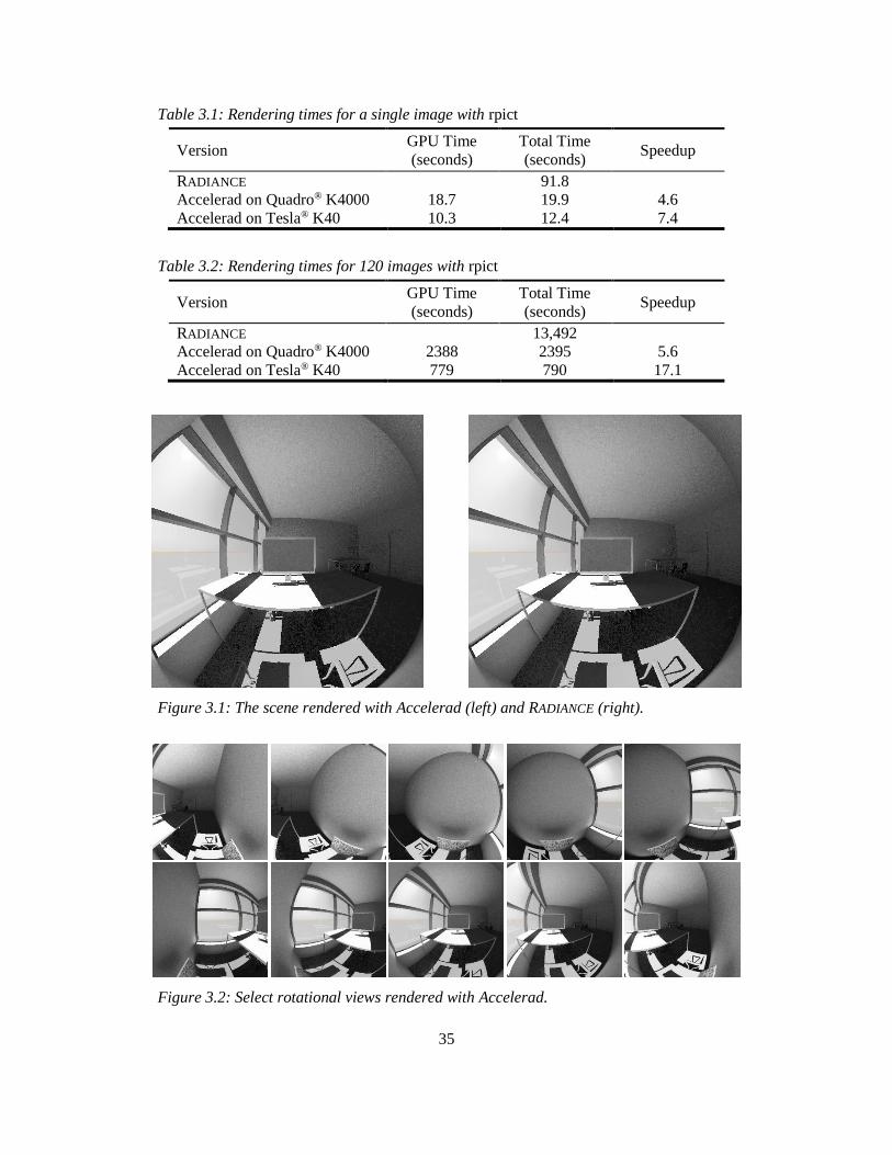
35

Table 3.1: Rendering times for a single image with rpict

Version GPU Time

(seconds)

Total Time

(seconds) Speedup

RADIANCE 91.8

Accelerad on Quadro® K4000 18.7 19.9 4.6

Accelerad on Tesla® K40 10.3 12.4 7.4

Table 3.2: Rendering times for 120 images with rpict

Version GPU Time

(seconds)

Total Time

(seconds) Speedup

RADIANCE 13,492

Accelerad on Quadro® K4000 2388 2395 5.6

Accelerad on Tesla® K40 779 790 17.1

Figure 3.1: The scene rendered with Accelerad (left) and RADIANCE (right).

Figure 3.2: Select rotational views rendered with Accelerad.

36

3.2.2 rtrace

While rpict demonstrates the coarse level of scalability achievable through rendering image sets, rtrace

shows finer scalability achievable by tracing large numbers of rays. The numeric output from rtrace also

demonstrates the fidelity with which Accelerad reproduces RADIANCE results.

In this test, we used the scene from Figure 3.1 again and cast rays from the camera position toward the

ceiling to sample radiance values. In order to increase coherence within warps, we used the same origin and

direction for all samples, though stochastic processes within the RADIANCE algorithms produce unique

results for each sample. While standard rtrace timings increase linearly with the number of primary rays at

a rate of 1.1×10-3 seconds per sample, Accelerad’s computation time is relatively constant for low numbers

of rays (Figure 3.3). Accelerad outperforms standard rtrace for simulations that take over 4 seconds on the

CPU. For large numbers of rays, Accelerad approaches a rate of 1.3×10-4 seconds per sample on the

Quadro® K4000, which represents an 89% marginal speed improvement over standard rtrace. The Tesla®

K40 performs even faster at 4.8×10-5 seconds per sample, giving it a 96% marginal speed improvement

over standard rtrace. While this scenario is admittedly constructed to achieve greater-than-usual coherence

within warps by repeatedly tracing the same ray, it demonstrates that Accelerad can run more than twenty

times faster than RADIANCE under certain conditions.

The timings achieved by maximizing coherence within warps should approach the theoretical maximum

speed of the ray tracing engine. This speed limit is dependent both on the scene and the hardware used.

However, random jitter applied to the directions of diffusely reflected rays causes divergence within the

Figure 3.3: Computation times for rtrace.

0.1

1

10

100

1000

10000

256 4096 65536 1048576

Tim

e (s

eco

nd

s)

Primary Rays

Radiance

Accelerad on Quadro K4000

Accelerad on Tesla K40

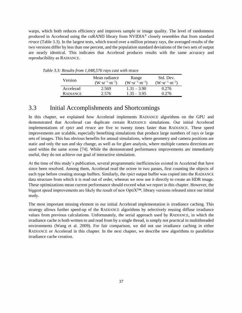
37

warps, which both reduces efficiency and improves sample or image quality. The level of randomness

produced in Accelerad using the cuRAND library from NVIDIA® closely resembles that from standard

rtrace (Table 3.3). In the largest tests, which traced over a million primary rays, the averaged results of the

two versions differ by less than one percent, and the population standard deviations of the two sets of output

are nearly identical. This indicates that Accelerad produces results with the same accuracy and

reproducibility as RADIANCE.

Table 3.3: Results from 1,048,576 rays cast with rtrace

Version Mean radiance

(W·sr−1·m−2)

Range

(W·sr−1·m−2)

Std. Dev.

(W·sr−1·m−2)

Accelerad 2.569 1.31 – 3.90 0.276

RADIANCE 2.576 1.35 – 3.95 0.276

3.3 Initial Accomplishments and Shortcomings

In this chapter, we explained how Accelerad implements RADIANCE algorithms on the GPU and

demonstrated that Accelerad can duplicate certain RADIANCE simulations. Our initial Accelerad

implementations of rpict and rtrace are five to twenty times faster than RADIANCE. These speed

improvements are scalable, especially benefiting simulations that produce large numbers of rays or large

sets of images. This has obvious benefits for annual simulations, where geometry and camera positions are

static and only the sun and sky change, as well as for glare analysis, where multiple camera directions are

used within the same scene [74]. While the demonstrated performance improvements are immediately

useful, they do not achieve our goal of interactive simulation.

At the time of this study’s publication, several programmatic inefficiencies existed in Accelerad that have

since been resolved. Among them, Accelerad read the octree in two passes, first counting the objects of

each type before creating storage buffers. Similarly, the rpict output buffer was copied into the RADIANCE

data structure from which it is read out of order, whereas we now use it directly to create an HDR image.

These optimizations mean current performance should exceed what we report in this chapter. However, the

biggest speed improvements are likely the result of new OptiX™, library versions released since our initial

study.

The most important missing element in our initial Accelerad implementation is irradiance caching. This

strategy allows further speed-up of the RADIANCE algorithms by selectively reusing diffuse irradiance

values from previous calculations. Unfortunately, the serial approach used by RADIANCE, in which the

irradiance cache is both written to and read from by a single thread, is simply not practical in multithreaded

environments (Wang et al. 2009). For fair comparison, we did not use irradiance caching in either

RADIANCE or Accelerad in this chapter. In the next chapter, we describe new algorithms to parallelize

irradiance cache creation.

39

4 Irradiance Caching

In the last chapter, we showed that the ray tracing performed by RADIANCE is highly parallelizable when

not using irradiance caching, a strategy that stores and retrieves results of expensive indirect irradiation

computations. This chapter describes a novel method of parallel multiple-bounce irradiance caching for

global illumination on a GPU. The chapter presents results from two investigations. The first study,

Irradiance caching for global illumination calculation on graphics hardware, was published in 2014 [12].

It describes our method for reading an irradiance cache on the GPU by mapping it to a bounding volume

hierarchy (BVH). It also describes how to create a fixed-size irradiance cache using a multi-stage method

on the GPU. This strategy can be adapted to fit various scenes and view types. Finally, we demonstrate the

effectiveness of our method on two scenes of vastly different scales in which it produces results up to twenty

times faster than RADIANCE with accuracy within RADIANCE’s ambient accuracy parameter.

The second study, Parallel multiple-bounce irradiance caching, was published in 2016 [13]. It presents an

algorithm for parallel construction of a dynamically sized irradiance cache over multiple-bounce paths.

Relevant points for irradiance calculation based on one or multiple cameras are located by tracing rays

through multiple-bounce paths. Irradiance values are then saved to a cache in reverse bounce order so that

the irradiance calculation at each bounce samples from previously calculated values. We show by

comparison to HDR photography of a moderately complex space that our method can predict luminance

distribution as accurately as RADIANCE, and that it is faster by an order of magnitude.

4.1 How It Works

While direct and specular reflections change abruptly over spatial dimensions, diffuse lighting due to

indirect irradiance is less variable. A single diffuse value may be applied to all ray intersections within a

calculated radius of the point where it was measured. An irradiance cache is a collection of diffuse

irradiance values and associated validity radii stored in a hierarchical acceleration structure (an octree in

RADIANCE) that allows them to be quickly retrieved based on geometric position and normal direction.

Given two cached irradiance values at points E1 and E2 in Figure 4.1, the irradiance at point A may be

found by interpolation, and the irradiance at point B may be found by extrapolation. Only when a ray

Figure 4.1 Irradiance cache records may be applied to all points within their valid radii

[114].

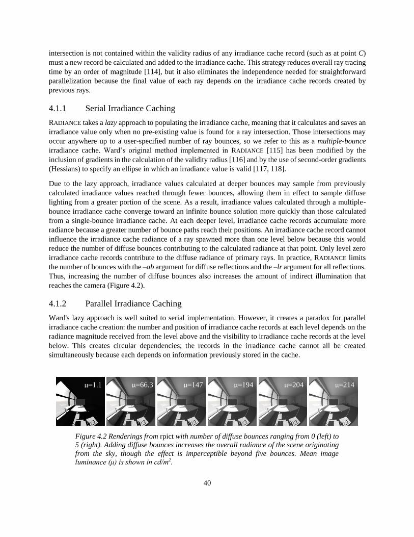
40

intersection is not contained within the validity radius of any irradiance cache record (such as at point C)

must a new record be calculated and added to the irradiance cache. This strategy reduces overall ray tracing

time by an order of magnitude [114], but it also eliminates the independence needed for straightforward

parallelization because the final value of each ray depends on the irradiance cache records created by

previous rays.

4.1.1 Serial Irradiance Caching

RADIANCE takes a lazy approach to populating the irradiance cache, meaning that it calculates and saves an

irradiance value only when no pre-existing value is found for a ray intersection. Those intersections may

occur anywhere up to a user-specified number of ray bounces, so we refer to this as a multiple-bounce

irradiance cache. Ward’s original method implemented in RADIANCE [115] has been modified by the

inclusion of gradients in the calculation of the validity radius [116] and by the use of second-order gradients

(Hessians) to specify an ellipse in which an irradiance value is valid [117, 118].

Due to the lazy approach, irradiance values calculated at deeper bounces may sample from previously

calculated irradiance values reached through fewer bounces, allowing them in effect to sample diffuse

lighting from a greater portion of the scene. As a result, irradiance values calculated through a multiple-

bounce irradiance cache converge toward an infinite bounce solution more quickly than those calculated

from a single-bounce irradiance cache. At each deeper level, irradiance cache records accumulate more

radiance because a greater number of bounce paths reach their positions. An irradiance cache record cannot

influence the irradiance cache radiance of a ray spawned more than one level below because this would

reduce the number of diffuse bounces contributing to the calculated radiance at that point. Only level zero

irradiance cache records contribute to the diffuse radiance of primary rays. In practice, RADIANCE limits

the number of bounces with the –ab argument for diffuse reflections and the –lr argument for all reflections.

Thus, increasing the number of diffuse bounces also increases the amount of indirect illumination that

reaches the camera (Figure 4.2).

4.1.2 Parallel Irradiance Caching

Ward's lazy approach is well suited to serial implementation. However, it creates a paradox for parallel

irradiance cache creation: the number and position of irradiance cache records at each level depends on the

radiance magnitude received from the level above and the visibility to irradiance cache records at the level

below. This creates circular dependencies; the records in the irradiance cache cannot all be created

simultaneously because each depends on information previously stored in the cache.

Figure 4.2 Renderings from rpict with number of diffuse bounces ranging from 0 (left) to

5 (right). Adding diffuse bounces increases the overall radiance of the scene originating

from the sky, though the effect is imperceptible beyond five bounces. Mean image

luminance (μ) is shown in cd/m2.

μ=1.1

8

μ=66.3 μ=147 μ=194 μ=204 μ=214

41

RADIANCE does allow multiple processes to write to a single cache using file locks [114]. Improved

synchronization methods use the Message-Passing Interface (MPI) [119, 120] and wait-free

synchronization [121]. Concurrent threads may calculate overlapping and redundant irradiance values, but

this happens infrequently so long as the number of threads is small.

In massively parallel systems, however, a lazy approach to populating the irradiance cache is likely to

produce many redundant entries. Modern GPUs implement single-instruction multiple-thread (SIMT)

architectures in which groups of 32 threads called warps simultaneously execute the same command on

different data. SIMT architecture allows threads within a warp to take divergent execution paths as a result

of the data they receive, but this reduces parallel efficiency, as some threads must idle while others perform

the divergent task [47]. Faster GPU ray tracing is achieved when the rays computed by each warp are

coherent, hitting the same triangles and calling the same intersection programs. If we were to implement

RADIANCE’s irradiance caching strategy directly on the GPU, it is highly likely that many threads in each

warp would attempt to create overlapping irradiance cache records, severely reducing computational

efficiency. Furthermore, adding records to the irradiance cache’s hierarchical acceleration structure can

require redistribution of nodes within the structure, leaving the irradiance cache temporarily unreadable to

threads from other warps.

A solution for massively parallel environments is to prefill the cache with entries that are likely to be

sampled; however, this requires a heuristic approach to determine where irradiance will need to be

calculated [93]. Various strategies have been proposed to completely prefill the irradiance cache. Splatting

[122] and pre-convolution [123] provide view-dependent solutions computed in screen space. Neighbor

clamping [124], Poisson-disk distribution [125], micro-rendering [126], and dithering combined with z-

curve clustering [127] can be used to place calculation points in world space, but consider only one diffuse

bounce. An adaptive seeding method by Wang et al. [128] uses quadtrees and k-means clustering to choose

irradiance calculation locations. It also considers only a single bounce within the irradiance cache, but the

irradiance values themselves come from photon mapping [129].

All of these existing methods have some limitations. Because they depend on the camera’s field of view to

determine irradiance cache record locations, they do not scale well to situations in which the camera moves

or rotates, such as in adaptive zone glare analysis [74]. They also assume that the rendered spaces are at

least mostly enclosed, and they provide no explicit mechanism for dealing with views to the exterior, which

are common in daylit scenes. We seek to address these shortcomings.

4.2 Fixed-Sized Caching Algorithms

On the GPU, we must read from and write to the irradiance cache at separate times. First, we discuss our

method for reading from the irradiance cache, which may be performed in conjunction with various

methods of irradiance cache creation. Then, we describe two methods for creating irradiance cache records

on the GPU, one optimized for small enclosed spaces and the other adapted to large open spaces.

4.2.1 Reading from an Irradiance Cache in Parallel

Whether or not we use the GPU for irradiance cache creation, we can save an irradiance cache to a binary

file to enable multiple simulations of a scene. Here, we describe how to use an existing irradiance cache in

OptiX™. Our first step is to enter all available level zero irradiance cache records into a BVH acceleration

structure. Each irradiance cache record represents a disc over which a given indirect irradiance value is

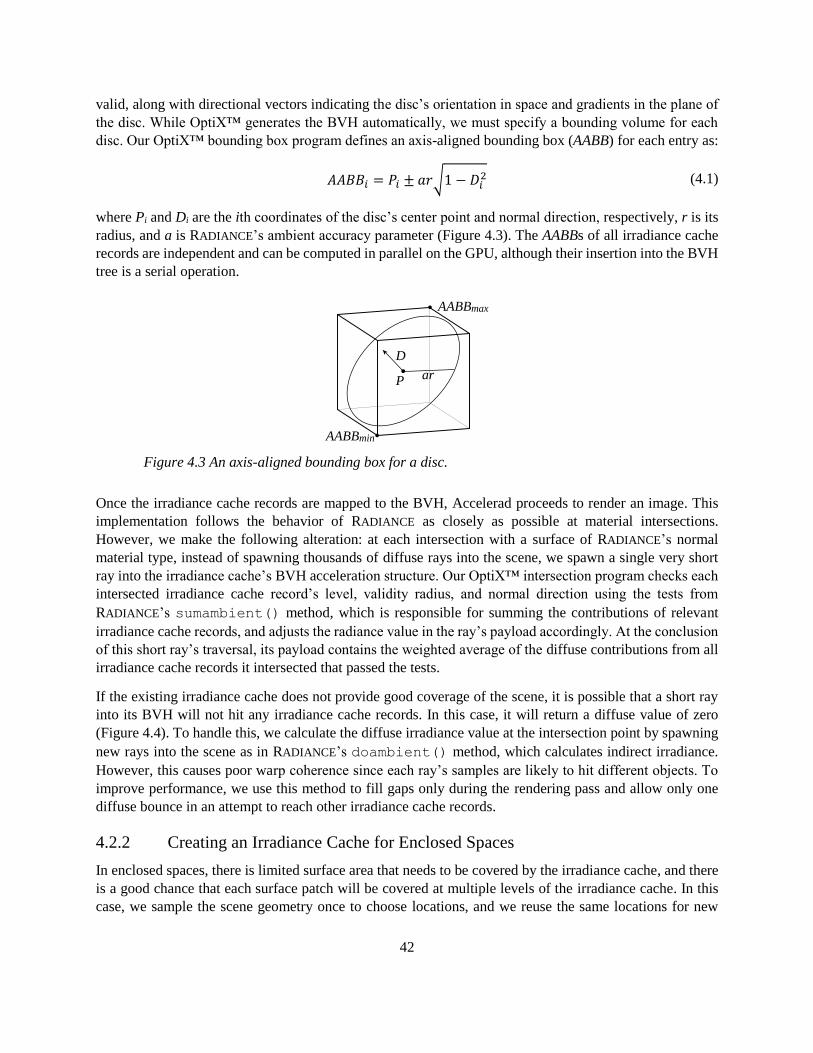
42

valid, along with directional vectors indicating the disc’s orientation in space and gradients in the plane of

the disc. While OptiX™ generates the BVH automatically, we must specify a bounding volume for each

disc. Our OptiX™ bounding box program defines an axis-aligned bounding box (AABB) for each entry as:

𝐴𝐴𝐵𝐵𝑖 = 𝑃𝑖 ± 𝑎𝑟√1 − 𝐷𝑖2 (4.1)

where Pi and Di are the ith coordinates of the disc’s center point and normal direction, respectively, r is its

radius, and a is RADIANCE’s ambient accuracy parameter (Figure 4.3). The AABBs of all irradiance cache

records are independent and can be computed in parallel on the GPU, although their insertion into the BVH

tree is a serial operation.

Figure 4.3 An axis-aligned bounding box for a disc.

Once the irradiance cache records are mapped to the BVH, Accelerad proceeds to render an image. This

implementation follows the behavior of RADIANCE as closely as possible at material intersections.

However, we make the following alteration: at each intersection with a surface of RADIANCE’s normal

material type, instead of spawning thousands of diffuse rays into the scene, we spawn a single very short

ray into the irradiance cache’s BVH acceleration structure. Our OptiX™ intersection program checks each

intersected irradiance cache record’s level, validity radius, and normal direction using the tests from

RADIANCE’s sumambient() method, which is responsible for summing the contributions of relevant

irradiance cache records, and adjusts the radiance value in the ray’s payload accordingly. At the conclusion

of this short ray’s traversal, its payload contains the weighted average of the diffuse contributions from all

irradiance cache records it intersected that passed the tests.

If the existing irradiance cache does not provide good coverage of the scene, it is possible that a short ray

into its BVH will not hit any irradiance cache records. In this case, it will return a diffuse value of zero

(Figure 4.4). To handle this, we calculate the diffuse irradiance value at the intersection point by spawning

new rays into the scene as in RADIANCE’s doambient() method, which calculates indirect irradiance.

However, this causes poor warp coherence since each ray’s samples are likely to hit different objects. To

improve performance, we use this method to fill gaps only during the rendering pass and allow only one

diffuse bounce in an attempt to reach other irradiance cache records.

4.2.2 Creating an Irradiance Cache for Enclosed Spaces

In enclosed spaces, there is limited surface area that needs to be covered by the irradiance cache, and there

is a good chance that each surface patch will be covered at multiple levels of the irradiance cache. In this

case, we sample the scene geometry once to choose locations, and we reuse the same locations for new

P

D

ar

AABBmin

AABBmax

43

irradiance cache records at each level. This eliminates the need to resample the scene geometry for each

irradiance cache level using additional OptiX™ kernel calls that can double the overall computation time.

We first sample the scene geometry to generate a list of location candidates, then reduce the number of

candidates while maintaining even scene coverage using k-means clustering, and finally create irradiance

cache records at each cluster in an iterative manner, proceeding from highest to lowest levels (Figure 4.5).

We feed the irradiance cache records for level zero into the rendering pass described in the previous section.

We create a list of location candidates for irradiance calculation based on geometry sampling. Using an

OptiX™ kernel, we cast rays from the eye position into the scene and record the position and surface normal

direction of the first hit point. If the eye position and field of view are to remain static, we choose the initial

ray directions to form a grid over the image using RADIANCE’s –vt argument and a user-specified sampling

density. If the eye rotates between images, as it does in glare analysis [74], we distribute the initial ray

directions over equal solid angle sections of a sphere. In order to include geometry that is not visible from

the eye position, we allow a user-defined number of bounces and record an additional position and normal

pair at each new intersection. For each bounce, a random cosine-weighted reflection direction is chosen

within the hemisphere defined by the surface normal. The output of this OptiX™ kernel is a list of points

and corresponding normal vectors that will be location candidates.

This list likely contains far more candidates than needed to cover the surfaces in the space, which could

cause excessive ray traversal times. Fortunately, we can reduce the list’s size by any of a number of

clustering methods. For simplicity, we perform iterative k-means clustering to find a user-defined number

of cluster centers using CUDA®, starting from a randomly chosen set of candidates. After clustering, the

location candidate nearest each cluster center will be used in the next step to generate an irradiance cache

record.

10 102 103 104 cd/m2

Figure 4.4 The scene with poor diffuse coverage (left) can be filled in during the rendering

pass (right). The figure shows tone mapped (top) and false color (bottom) images.

44

Figure 4.5 In enclosed spaces, locations from a single call to the sampling kernel are used

to create the irradiance cache (IC) at each level.

The k-means algorithm requires a distance metric in order to cluster nearby objects. In this case, the metric

must consider not only Euclidian distance, but also the normal discrepancy between candidates. We use the

modification by Wang et al. [128] of the error in the split sphere model [116]:

𝜀 = 𝛼‖𝑥𝑖 − 𝑥𝑘‖ + √2 − 2(𝑛𝑖 ∙ 𝑛𝑘) (4.2)

to relate error ε to the change in position x and normal direction n from candidate i to cluster center k, given

a user-defined weighting factor α that accounts for scene size. This modified error metric is preferable

because it can be used without calculating the indirect irradiance at every candidate location.

The irradiance cache is built through iterative calls to a diffuse sampling OptiX™ kernel. Each call to this

kernel creates one irradiance cache record for each chosen location candidate in parallel. The process is

similar to RADIANCE’s doambient() method, which computes the indirect irradiance at a point by

sampling the scene geometry with rays, except that no supersampling takes place because OptiX™ does

not provide an efficient sorting mechanism or memory to store a large number of diffuse samples per thread.

This is acceptable because the cost of using a large number of ambient divisions is much lower on the GPU

than on the CPU. The first call to the kernel creates the highest irradiance cache level by sampling the

environment with no diffuse bounces. After each kernel call, the new irradiance cache records are entered

into a BVH using the AABB described in the previous section. Subsequent calls to the kernel repeat the

indirect irradiance calculation at each location by sampling the irradiance cache from the previous round.

The irradiance cache generated at level zero is used to create the final image as previously described.

4.2.3 Creating an Irradiance Cache for Open Spaces

In open spaces, higher-level irradiance cache records are likely to be spread out geometrically, while lower-

level records will tend to cluster near the eye position. This differs from the previous case in that we must

now choose different record locations for each irradiance cache level in order to achieve optimal coverage

for each diffuse bounce (Figure 4.6). We make three changes to the method described in the previous

section. First, the kernel used initially to sample the scene geometry generates only one point-normal pair

45

per GPU thread because no bounces are needed. The candidate locations, again chosen by k-means

clustering, serve as the locations for only the irradiance cache records at level zero. Second, we introduce

a new geometry sampling OptiX™ kernel that spawns rays from the previous cluster centers to identify

new location candidates using RADIANCE’s ambient sampling distribution. The point-normal pairs from

this kernel also undergo k-means clustering, and the results are used both as locations for level one

irradiance cache records and as new input to the same kernel. This process recurses through the number of

iterations specified by RADIANCE’s –ab argument. Third, while the irradiance cache creation kernel is still

called once per level as in the previous section, it now receives a different set of input locations on each

call, consuming both the cluster centers from the corresponding level and the irradiance cache from its

previous invocation. As before, the level zero irradiance cache serves as input to the rendering pass.

4.3 Validation of the Fixed-Sized Irradiance Cache

We demonstrate the speed and accuracy of Accelerad’s implementation of a fixed-sized irradiance cache

by comparing it to RADIANCE’s rpict program for two scenes. The first, a fictitious small furnished office

composed of 278,695 triangles, fits the criteria for an enclosed space. The second, a model of Harvard

University’s Gund Hall with 187,208 triangles, is characteristic of open spaces. We calculate the speedup

factor as the ratio of rpict computation time to the computation time of Accelerad’s implementation with

the same number of diffuse bounces. In order to quantify the error introduced by our method, we report the

mean radiance of the image generated by Accelerad as a percentage of the mean radiance in the RADIANCE

image with the most diffuse bounces. This is an imperfect metric because rpict does produce rendering

artifacts, but it serves to demonstrate the extent of agreement between classic RADIANCE and Accelerad.

We ran simulations on two machines. The first was an active workstation with a 3.4 GHz Intel® Core™ i7-

4770 processor and an NVIDIA® Quadro® K4000 graphics card with 768 CUDA® cores. The second was

a dedicated graphics workstation with a 2.27 GHz Intel® Xeon® E5520 processor and two NVIDIA® Tesla®

Figure 4.6 In open spaces, irradiance cache (IC) record locations are separately

calculated for each irradiance cache level based on locations reached at the previous

level.

46

K40 graphics accelerators with 2880 CUDA® cores each. We configured Accelerad to use either one or

both accelerators. We ran RADIANCE only on the first machine with the faster processor.

4.3.1 Enclosed Space

We rendered the small office scene with varying numbers of diffuse bounces in both RADIANCE and

Accelerad (Figure 4.7). Using an ambient accuracy of 5%, minimum ray weight of 0.2%, and 3000 ambient

divisions, the number of rays cast by rpict leveled off at 1.28×108 after five diffuse bounces, which took

46.5 minutes. We take five diffuse bounces to be optimal for this scene with these settings.

We rendered the small office scene with Accelerad using methods for both enclosed and open spaces. The

enclosed method returned results in half the time of the open method for tests with 4096 or more clusters.

Because irradiance caches of this size provide good coverage of the small scene, the two methods have

comparable accuracy. As a result, we report only the performance of the faster enclosed method.

As with RADIANCE, Accelerad’s rendering time increases and its error decreases until five diffuse bounces,

after which they become essentially constant (Figure 4.8). Because IC records at higher levels can be built

using exponentially fewer rays, the speedup factor is greater for higher numbers of bounces, reaching a

maximum of 17 times rpict’s speed when using 4096 clusters.

Increasing the number of clusters also reduces error, though the effect on speed is more complicated. Low

cluster counts result in reduced ambient coverage, which produces work that is more incoherent during the

rendering pass, increasing computation time. High cluster counts increase the time for ray traversal of the

irradiance cache’s BVH. Using five diffuse bounces, a 24-fold speedup can be achieved with 2048 clusters

per irradiance cache level, but increased accuracy can be achieved with more clusters.

10 102 103 104 cd/m2

Figure 4.7 The small office scene rendered with five diffuse bounces with RADIANCE (left)

and 17 times faster with Accelerad (right).

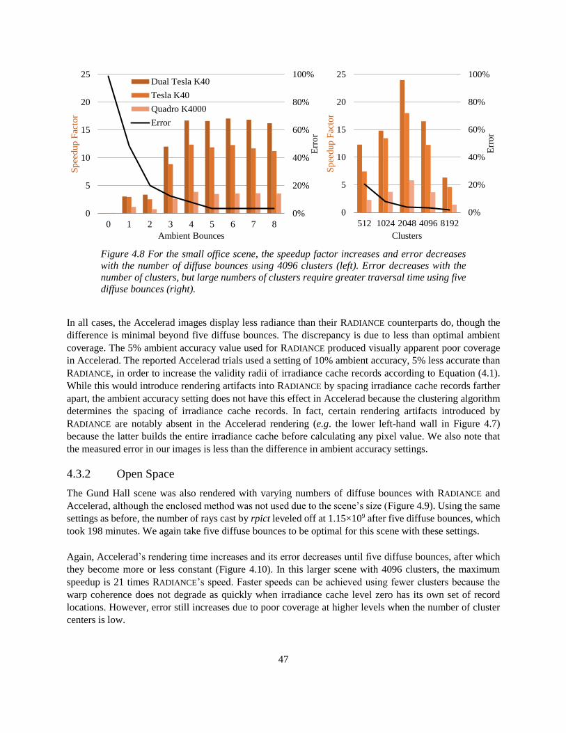
47

In all cases, the Accelerad images display less radiance than their RADIANCE counterparts do, though the

difference is minimal beyond five diffuse bounces. The discrepancy is due to less than optimal ambient

coverage. The 5% ambient accuracy value used for RADIANCE produced visually apparent poor coverage

in Accelerad. The reported Accelerad trials used a setting of 10% ambient accuracy, 5% less accurate than

RADIANCE, in order to increase the validity radii of irradiance cache records according to Equation (4.1).

While this would introduce rendering artifacts into RADIANCE by spacing irradiance cache records farther

apart, the ambient accuracy setting does not have this effect in Accelerad because the clustering algorithm

determines the spacing of irradiance cache records. In fact, certain rendering artifacts introduced by

RADIANCE are notably absent in the Accelerad rendering (e.g. the lower left-hand wall in Figure 4.7)

because the latter builds the entire irradiance cache before calculating any pixel value. We also note that

the measured error in our images is less than the difference in ambient accuracy settings.

4.3.2 Open Space

The Gund Hall scene was also rendered with varying numbers of diffuse bounces with RADIANCE and

Accelerad, although the enclosed method was not used due to the scene’s size (Figure 4.9). Using the same

settings as before, the number of rays cast by rpict leveled off at 1.15×109 after five diffuse bounces, which

took 198 minutes. We again take five diffuse bounces to be optimal for this scene with these settings.

Again, Accelerad’s rendering time increases and its error decreases until five diffuse bounces, after which

they become more or less constant (Figure 4.10). In this larger scene with 4096 clusters, the maximum

speedup is 21 times RADIANCE’s speed. Faster speeds can be achieved using fewer clusters because the

warp coherence does not degrade as quickly when irradiance cache level zero has its own set of record

locations. However, error still increases due to poor coverage at higher levels when the number of cluster

centers is low.

Figure 4.8 For the small office scene, the speedup factor increases and error decreases

with the number of diffuse bounces using 4096 clusters (left). Error decreases with the

number of clusters, but large numbers of clusters require greater traversal time using five

diffuse bounces (right).

0%

20%

40%

60%

80%

100%

0

5

10

15

20

25

0 1 2 3 4 5 6 7 8

Err

or

Sp

eed

up

Fac

tor

Ambient Bounces

Dual Tesla K40

Tesla K40

Quadro K4000

Error

0%

20%

40%

60%

80%

100%

0

5

10

15

20

25

512 1024 2048 4096 8192

Err

or

Sp

eed

up

Fac

tor

Clusters

48

The increased error in the Gund Hall scene indicates that coverage is generally poorer here than in the small

office scene. This is to be expected, given that Gund Hall is a larger space. To offset this effect, the

Accelerad renderings use an ambient accuracy setting of 25% to increase irradiance cache record validity

radii. This ultimately produces a 17% difference in mean radiance between RADIANCE and Accelerad with

4096 clusters. While this error appears large, some of it must be attributed to rendering artifacts produced

by RADIANCE (e.g. under the table in Figure 4.10). We again note that the error observed is less than the

20% difference between the Accelerad and RADIANCE ambient accuracy settings.

4.4 The Problem of Coverage

In the first half of this chapter, we have demonstrated that irradiance caching, along with other core

algorithms from RADIANCE, can be implemented using OptiX™ to achieve a twenty-fold speed increase in

global illumination simulation. By precomputing a separate irradiance cache for each diffuse bounce level,

we can duplicate RADIANCE rpict results with reasonable accuracy. In enclosed spaces, we can further

reduce computation time by reusing the same locations for irradiance cache records at each level.

The primary source of error at this preliminary stage of development is poor ambient coverage of the scene.

We have shown that in enclosed spaces, irradiance caches that provide good scene coverage can be

generated in parallel on the GPU. However, the user remains responsible for predicting the necessary size

of the irradiance cache, which is impractical in most real cases and prohibits widespread adoption of the

method. Unfortunately, poor cache sizing lead either to under- or over-coverage of the scene, which in

either case can severely increase rendering times. In the second half of this chapter, we present a method to

determine the appropriate number and placement of irradiance cache records to maximize scene coverage.

10 102 103 104 cd/m2

Figure 4.9 The Gund Hall scene rendered with five diffuse bounces with RADIANCE (left)

and 20 times faster with Accelerad (right).

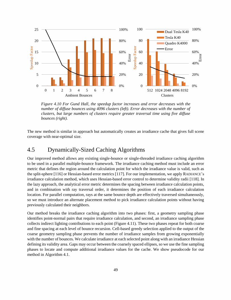
49

The new method is similar in approach but automatically creates an irradiance cache that gives full scene

coverage with near-optimal size.

4.5 Dynamically-Sized Caching Algorithms

Our improved method allows any existing single-bounce or single-threaded irradiance caching algorithm

to be used in a parallel multiple-bounce framework. The irradiance caching method must include an error

metric that defines the region around the calculation point for which the irradiance value is valid, such as

the split-sphere [116] or Hessian-based error metrics [117]. For our implementation, we apply RADIANCE’s

irradiance calculation method, which uses Hessian-based error control to determine validity radii [118]. In

the lazy approach, the analytical error metric determines the spacing between irradiance calculation points,

and in combination with ray traversal order, it determines the position of each irradiance calculation

location. For parallel computation, rays at the same bounce depth are effectively traversed simultaneously,

so we must introduce an alternate placement method to pick irradiance calculation points without having

previously calculated their neighbors.

Our method breaks the irradiance caching algorithm into two phases: first, a geometry sampling phase

identifies point-normal pairs that require irradiance calculation, and second, an irradiance sampling phase

collects indirect lighting contributions to each point (Figure 4.11). These two phases repeat for both coarse

and fine spacing at each level of bounce recursion. Cell-based greedy selection applied to the output of the

coarse geometry sampling phase prevents the number of irradiance samples from growing exponentially

with the number of bounces. We calculate irradiance at each selected point along with an irradiance Hessian

defining its validity area. Gaps may occur between the coarsely spaced ellipses, so we use the fine sampling

phases to locate and compute additional irradiance values for the cache. We show pseudocode for our

method in Algorithm 4.1.

Figure 4.10 For Gund Hall, the speedup factor increases and error decreases with the

number of diffuse bounces using 4096 clusters (left). Error decreases with the number of

clusters, but large numbers of clusters require greater traversal time using five diffuse

bounces (right).

0%

20%

40%

60%

80%

100%

0

5

10

15

20

25

0 1 2 3 4 5 6 7 8

Err

or

Sp

eed

up

Fac

tor

Ambient Bounces

0%

20%

40%

60%

80%

100%

0

20

40

60

80

100

512 1024 2048 4096 8192

Err

or

Sp

eed

up

Fac

tor

Clusters

Dual Tesla K40

Tesla K40

Quadro K4000

Error

50

Figure 4.11 The dynamically sized irradiance cache (IC) replaces k-means clustering with

cell-based clustering and repeats the first sampling pass with a fine pass at each level.

Algorithm 4.1 Parallel multiple bounce irradiance caching algorithm

1 procedure BUILD IRRADIANCE CACHE

2 level = 0

3 points[0] = eye

4 cache[levelmax] = ∅

5 while level < levelmax do

6 temp = sample geometry seen from points[level] ► coarse geometry sampling

7 Sort temp by cell index

8 Increment level

9 points[level] = rcoarse-spaced points from temp

10 end while

11 while level > 0 do

12 Decrement level

13 cache[level] = sample irradiance from cache[level + 1] at points[level + 1] ► coarse irradiance sampling

14 temp = sample geometry seen from points[level] ► fine geometry sampling

15 Sort temp by cell index

16 points[level + 1] = rmin-spaced points from temp

17 cache[level] += sample irradiance from cache[level + 1] at points[level + 1] ► fine irradiance sampling

18 end while

19 end procedure

4.5.1 Coarse Geometry Sampling

The first step is to find point-normal pairs at which irradiance will later be calculated. Unlike the lazy

approach, we identify point-normal pairs in advance rather than on an as-needed basis. As a result, the

validity radius of each irradiance value and thus the appropriate spacing between point-normal pairs is not

known. We assume a user-defined lower limit on validity radii rmin; in practice, RADIANCE users choose

this limit based on rules of thumb. We could space calculation points by a distance of rmin in order to

guarantee complete coverage, but this would create an excessively large irradiance cache. Instead, we use

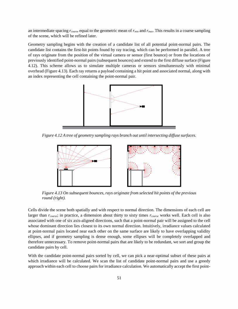
51

an intermediate spacing rcoarse equal to the geometric mean of rmin and rmax. This results in a coarse sampling

of the scene, which will be refined later.

Geometry sampling begins with the creation of a candidate list of all potential point-normal pairs. The

candidate list contains the first-hit points found by ray tracing, which can be performed in parallel. A tree

of rays originate from the position of the virtual camera or sensor (first bounce) or from the locations of

previously identified point-normal pairs (subsequent bounces) and extend to the first diffuse surface (Figure

4.12). This scheme allows us to simulate multiple cameras or sensors simultaneously with minimal

overhead (Figure 4.13). Each ray returns a payload containing a hit point and associated normal, along with

an index representing the cell containing the point-normal pair.

Figure 4.12 A tree of geometry sampling rays branch out until intersecting diffuse surfaces.

Figure 4.13 On subsequent bounces, rays originate from selected hit points of the previous

round (right).

Cells divide the scene both spatially and with respect to normal direction. The dimensions of each cell are

larger than rcoarse; in practice, a dimension about thirty to sixty times rcoarse works well. Each cell is also

associated with one of six axis-aligned directions, such that a point-normal pair will be assigned to the cell

whose dominant direction lies closest to its own normal direction. Intuitively, irradiance values calculated

at point-normal pairs located near each other on the same surface are likely to have overlapping validity

ellipses, and if geometry sampling is dense enough, some ellipses will be completely overlapped and

therefore unnecessary. To remove point-normal pairs that are likely to be redundant, we sort and group the

candidate pairs by cell.

With the candidate point-normal pairs sorted by cell, we can pick a near-optimal subset of these pairs at

which irradiance will be calculated. We scan the list of candidate point-normal pairs and use a greedy

approach within each cell to choose pairs for irradiance calculation. We automatically accept the first point-

52

normal pair in each cell. We accept additional point-normal pairs if they are located at least rcoarse away

from all previously accepted pairs in the same cell or if their normal direction differs by more than a user-

specified deviation, defaulting to 0.2 radians. While this directional deviation test is not optimal, it has

produced good results previously [118] and does not cause misses because we use it at other times that we

search the irradiance cache as well. We save the selected point-normal pairs as origins for later irradiance

calculation and more immediately as origins for geometry sampling at the next bounce.

4.5.2 Coarse Irradiance Sampling

Once we complete coarse geometry sampling for all bounces, we begin irradiance calculation starting with

the deepest bounce. Any irradiance calculation method may be used; our implementation uses jittered

Shirley-Chiu radiance sampling [130] with Hessian-based validity ellipses as implemented in RADIANCE

[118]. We trace irradiance sampling rays only to their first hit point, where we sample either direct

irradiation only (at the deepest bounce) or direct irradiation and cached irradiance values from the next

deeper bounce (at all other bounces).

Hessian-based irradiance calculation determines an elliptical area for which the irradiance value holds with

major and minor radii 𝑅𝑖𝜆1 and 𝑅𝑖

𝜆2 defined as follows [117]:

(𝑅𝑖𝜆1 , 𝑅𝑖

𝜆2) ≈ √4𝜀𝑡

𝜋

4

(√1

𝜆1

4

, √1

𝜆2

4

) (4.3)

where 𝜆1 and 𝜆2 are the eigenvalues of the irradiance Hessian matrix and εt is the user-defined total

allowable error. We bound the radii between rmin and rmax to prevent under- or over-sampling, respectively.

If the minor radius of the ellipse is less than rcoarse, then some relevant portions of the scene may not be

covered by any cached irradiance value, and irradiance sampling at the next bounce closer to the eye could

encounter holes. To prevent this, we insert a fine sampling phase before proceeding to the next bounce.

4.5.3 Fine Geometry Sampling

The fine geometry sampling phase proceeds much like the coarse version with a few exceptions. First,

during the parallel ray casting, we ignore first hit points if they fall within the validity ellipse of an irradiance

value calculated during coarse irradiance sampling at the same bounce. We can still use these points as

locations for specular reflections, however. Second, we use a smaller spacing to pick point-normal pairs

within each cell. In principle, the spacing should be rmin to guarantee complete coverage of the scene;

however, in many cases, we can achieve complete coverage with a larger spacing, as the validity radius will

only reach its lower limit near edges under low light levels. Finally, because of the smaller spacing, we also

use a smaller cell size. Typically, a cell edge length thirty to sixty times rmin works well.

4.5.4 Fine Irradiance Sampling

Irradiance calculation for fine sampling works the same as for coarse irradiance sampling with validity

areas defined by Equation (4.3). The origin points are those identified by the fine geometry sampling phase.

We skip this phase if the fine geometry sampling phase identified no new points, which may happen if the

irradiance values calculated in the coarse phase all have minor elliptical radii greater than rcoarse.

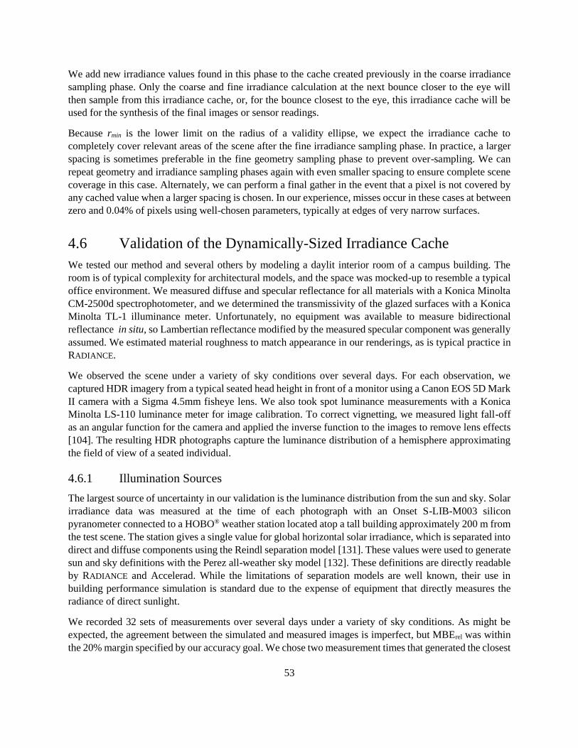
53

We add new irradiance values found in this phase to the cache created previously in the coarse irradiance

sampling phase. Only the coarse and fine irradiance calculation at the next bounce closer to the eye will

then sample from this irradiance cache, or, for the bounce closest to the eye, this irradiance cache will be

used for the synthesis of the final images or sensor readings.

Because rmin is the lower limit on the radius of a validity ellipse, we expect the irradiance cache to

completely cover relevant areas of the scene after the fine irradiance sampling phase. In practice, a larger

spacing is sometimes preferable in the fine geometry sampling phase to prevent over-sampling. We can

repeat geometry and irradiance sampling phases again with even smaller spacing to ensure complete scene

coverage in this case. Alternately, we can perform a final gather in the event that a pixel is not covered by

any cached value when a larger spacing is chosen. In our experience, misses occur in these cases at between

zero and 0.04% of pixels using well-chosen parameters, typically at edges of very narrow surfaces.

4.6 Validation of the Dynamically-Sized Irradiance Cache

We tested our method and several others by modeling a daylit interior room of a campus building. The

room is of typical complexity for architectural models, and the space was mocked-up to resemble a typical

office environment. We measured diffuse and specular reflectance for all materials with a Konica Minolta

CM-2500d spectrophotometer, and we determined the transmissivity of the glazed surfaces with a Konica

Minolta TL-1 illuminance meter. Unfortunately, no equipment was available to measure bidirectional

reflectance in situ, so Lambertian reflectance modified by the measured specular component was generally

assumed. We estimated material roughness to match appearance in our renderings, as is typical practice in

RADIANCE.

We observed the scene under a variety of sky conditions over several days. For each observation, we

captured HDR imagery from a typical seated head height in front of a monitor using a Canon EOS 5D Mark

II camera with a Sigma 4.5mm fisheye lens. We also took spot luminance measurements with a Konica

Minolta LS-110 luminance meter for image calibration. To correct vignetting, we measured light fall-off

as an angular function for the camera and applied the inverse function to the images to remove lens effects

[104]. The resulting HDR photographs capture the luminance distribution of a hemisphere approximating

the field of view of a seated individual.

4.6.1 Illumination Sources

The largest source of uncertainty in our validation is the luminance distribution from the sun and sky. Solar

irradiance data was measured at the time of each photograph with an Onset S-LIB-M003 silicon

pyranometer connected to a HOBO® weather station located atop a tall building approximately 200 m from

the test scene. The station gives a single value for global horizontal solar irradiance, which is separated into

direct and diffuse components using the Reindl separation model [131]. These values were used to generate

sun and sky definitions with the Perez all-weather sky model [132]. These definitions are directly readable

by RADIANCE and Accelerad. While the limitations of separation models are well known, their use in

building performance simulation is standard due to the expense of equipment that directly measures the

radiance of direct sunlight.

We recorded 32 sets of measurements over several days under a variety of sky conditions. As might be

expected, the agreement between the simulated and measured images is imperfect, but MBErel was within

the 20% margin specified by our accuracy goal. We chose two measurement times that generated the closest

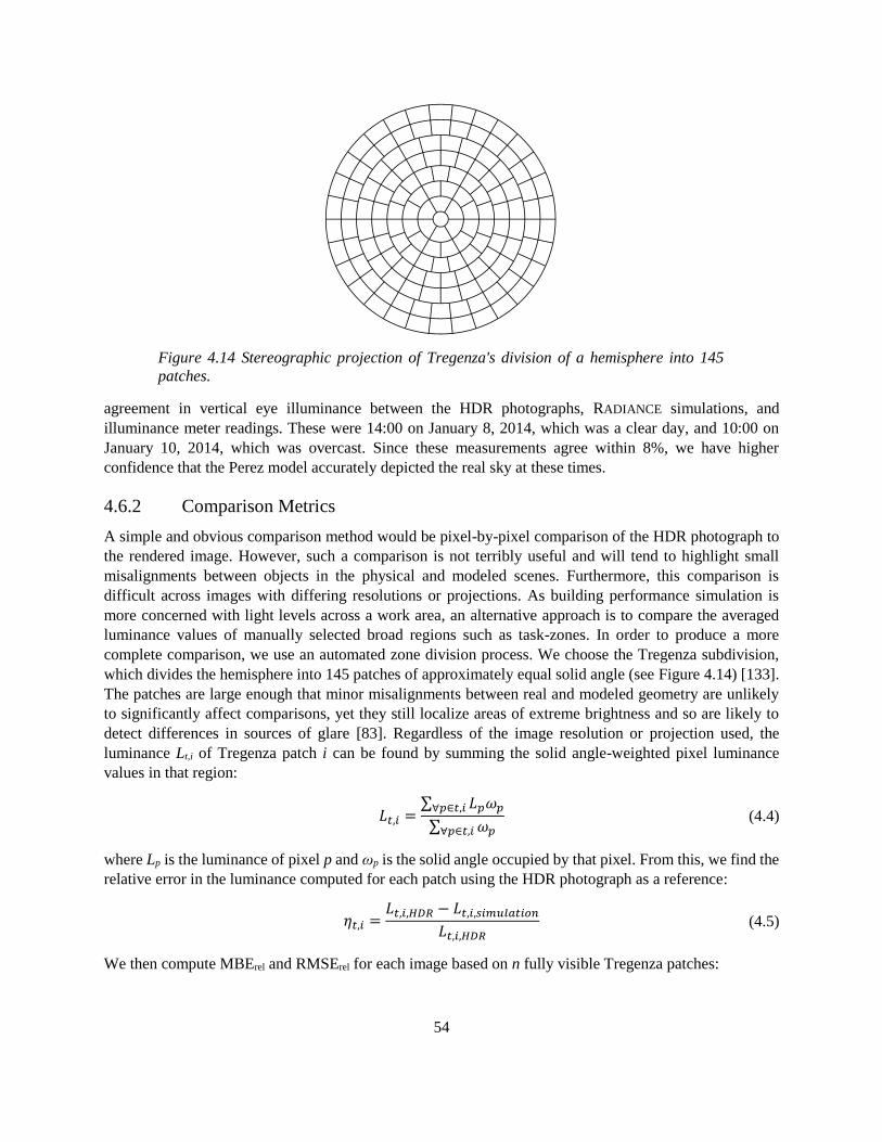
54

agreement in vertical eye illuminance between the HDR photographs, RADIANCE simulations, and

illuminance meter readings. These were 14:00 on January 8, 2014, which was a clear day, and 10:00 on

January 10, 2014, which was overcast. Since these measurements agree within 8%, we have higher

confidence that the Perez model accurately depicted the real sky at these times.

4.6.2 Comparison Metrics

A simple and obvious comparison method would be pixel-by-pixel comparison of the HDR photograph to

the rendered image. However, such a comparison is not terribly useful and will tend to highlight small

misalignments between objects in the physical and modeled scenes. Furthermore, this comparison is

difficult across images with differing resolutions or projections. As building performance simulation is

more concerned with light levels across a work area, an alternative approach is to compare the averaged

luminance values of manually selected broad regions such as task-zones. In order to produce a more

complete comparison, we use an automated zone division process. We choose the Tregenza subdivision,

which divides the hemisphere into 145 patches of approximately equal solid angle (see Figure 4.14) [133].

The patches are large enough that minor misalignments between real and modeled geometry are unlikely

to significantly affect comparisons, yet they still localize areas of extreme brightness and so are likely to

detect differences in sources of glare [83]. Regardless of the image resolution or projection used, the

luminance Lt,i of Tregenza patch i can be found by summing the solid angle-weighted pixel luminance

values in that region:

𝐿𝑡,𝑖 =∑ 𝐿𝑝𝜔𝑝∀𝑝∈𝑡,𝑖

∑ 𝜔𝑝∀𝑝∈𝑡,𝑖 (4.4)

where Lp is the luminance of pixel p and ωp is the solid angle occupied by that pixel. From this, we find the

relative error in the luminance computed for each patch using the HDR photograph as a reference:

𝜂𝑡,𝑖 =𝐿𝑡,𝑖,𝐻𝐷𝑅 − 𝐿𝑡,𝑖,𝑠𝑖𝑚𝑢𝑙𝑎𝑡𝑖𝑜𝑛

𝐿𝑡,𝑖,𝐻𝐷𝑅 (4.5)

We then compute MBErel and RMSErel for each image based on n fully visible Tregenza patches:

Figure 4.14 Stereographic projection of Tregenza's division of a hemisphere into 145

patches.

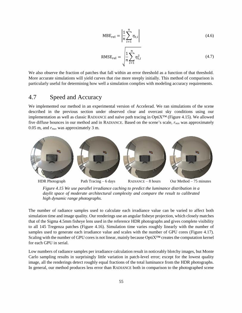
55

MBErel = |1

𝑛∑𝜂𝑡,𝑖

𝑛

𝑖=1

| (4.6)

RMSErel = √1

𝑛∑𝜂𝑡,𝑖

2

𝑛

𝑖=1

(4.7)

We also observe the fraction of patches that fall within an error threshold as a function of that threshold.

More accurate simulations will yield curves that rise more steeply initially. This method of comparison is

particularly useful for determining how well a simulation complies with modeling accuracy requirements.

4.7 Speed and Accuracy

We implemented our method in an experimental version of Accelerad. We ran simulations of the scene

described in the previous section under observed clear and overcast sky conditions using our

implementation as well as classic RADIANCE and naïve path tracing in OptiX™ (Figure 4.15). We allowed

five diffuse bounces in our method and in RADIANCE. Based on the scene’s scale, rmin was approximately

0.05 m, and rmax was approximately 3 m.

HDR Photograph Path Tracing – 6 days RADIANCE – 8 hours Our Method – 75 minutes

Figure 4.15 We use parallel irradiance caching to predict the luminance distribution in a

daylit space of moderate architectural complexity and compare the result to calibrated

high dynamic range photographs.

The number of radiance samples used to calculate each irradiance value can be varied to affect both

simulation time and image quality. Our renderings use an angular fisheye projection, which closely matches

that of the Sigma 4.5mm fisheye lens used in the reference HDR photographs and gives complete visibility

to all 145 Tregenza patches (Figure 4.16). Simulation time varies roughly linearly with the number of

samples used to generate each irradiance value and scales with the number of GPU cores (Figure 4.17).

Scaling with the number of GPU cores is not linear, mainly because OptiX™ creates the computation kernel

for each GPU in serial.

Low numbers of radiance samples per irradiance calculation result in noticeably blotchy images, but Monte

Carlo sampling results in surprisingly little variation in patch-level error; except for the lowest quality

image, all the renderings detect roughly equal fractions of the total luminance from the HDR photographs.

In general, our method produces less error than RADIANCE both in comparison to the photographed scene

56

and to path tracing (Figure 4.18). We used an overture pass to smooth irradiance caching artifacts in the

RADIANCE images, which had a negligible effect on patch-level errors. The path-traced images were

HDR Photo 16 64 256 512 1024 2048

Cle

ar S

ky

Dif

fere

nce

+500 cd/m2

-500 cd/m2

Ov

erca

st S

ky

Dif

fere

nce

+500 cd/m2

-500 cd/m2

Figure 4.16 The scene captured by HDR photography (left column) and rendered by our

method with varying numbers of radiance samples per irradiance calculation seen in

180° fisheye projection.

Figure 4.17 Simulation time as a function of sampling rate. Our method ran on one or

two NVIDIA® Tesla® K40 GPUs. RADIANCE ran on one 3.4 GHz core.

0

100

200

300

400

500

0 512 1024 1536 2048

Tim

e (m

inute

s)

Radiance Samples per Irradiance Calculation

Clear – 2x Tesla K40Overcast – 2x Tesla K40Clear – 1x Tesla K40Overcast – 1x Tesla K40Clear – RadianceOvercast – Radiance

57

allowed to render until diffuse noise artifacts disappeared, although the variation in patch-level error over

the duration of the run was minimal. Error in the path-traced images is attributable to discrepancies between

actual and modeled geometry, materials, and sky luminance distributions.

Higher numbers of radiance samples per irradiance calculation result do increase the number of Tregenza

patches within an error threshold (Figure 4.19). For both sky conditions with any given error tolerance,

simulations that use more radiance samples produce more patches within the tolerance. The advantage is

especially apparent for the clear sky simulation at very low tolerances. However, the additional samples

yield diminishing returns, and it seems unlikely that increasing beyond 2048 samples per irradiance

calculation will yield much benefit.

Figure 4.18 MBErel and RMSErel in luminance relative to measured values as a function

of sampling rate.

0.2

0.3

0.4

0.5

0 512 1024 1536 2048

RM

SE

rel

0

0.1

0.2

0 512 1024 1536 2048

MB

Ere

l

Radiance Samples per Irradiance Calculation

Clear – Our Method Overcast – Our MethodClear – Radiance Overcast – RadianceClear – Path Tracing Overcast – Path Tracing

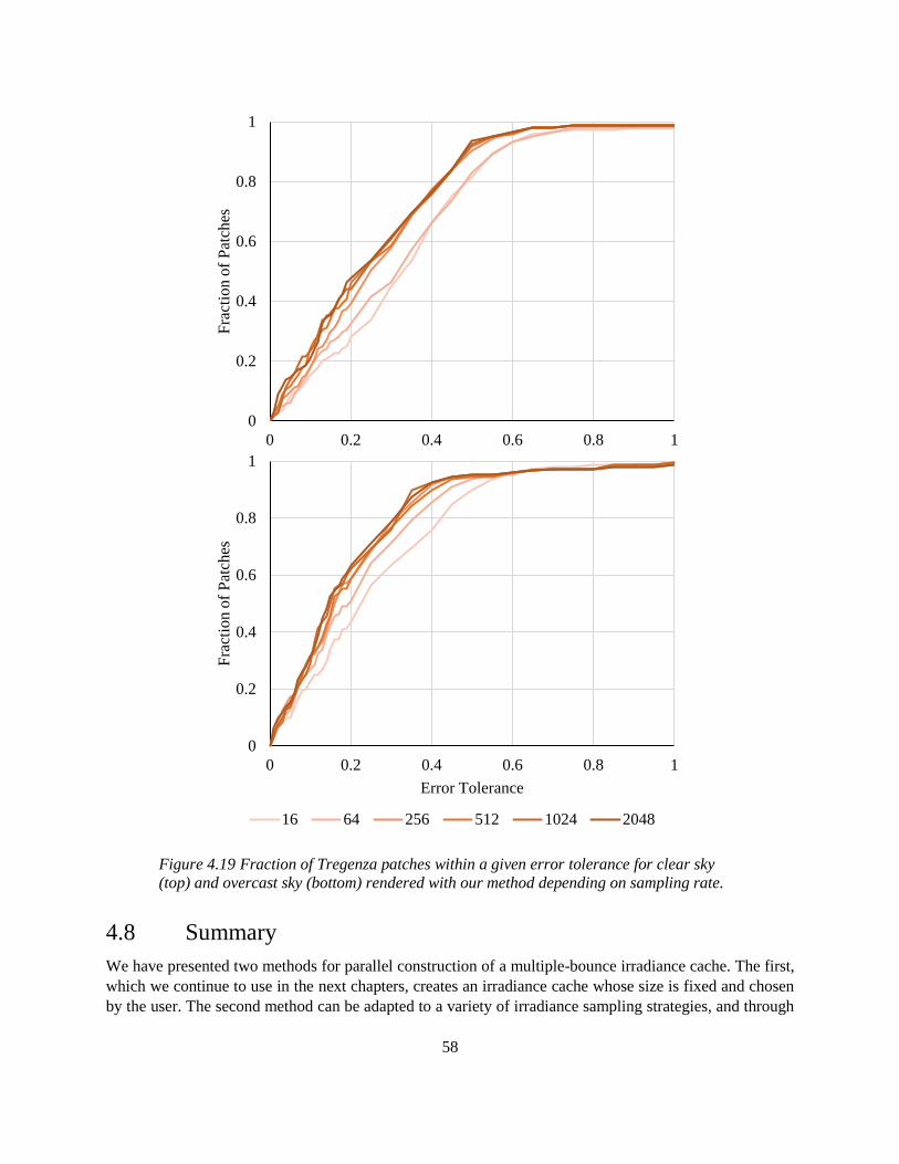
58

Figure 4.19 Fraction of Tregenza patches within a given error tolerance for clear sky

(top) and overcast sky (bottom) rendered with our method depending on sampling rate.

4.8 Summary

We have presented two methods for parallel construction of a multiple-bounce irradiance cache. The first,

which we continue to use in the next chapters, creates an irradiance cache whose size is fixed and chosen

by the user. The second method can be adapted to a variety of irradiance sampling strategies, and through

0

0.2

0.4

0.6

0.8

1

0 0.2 0.4 0.6 0.8 1

Fra

ctio

n o

f P

atch

es

0

0.2

0.4

0.6

0.8

1

0 0.2 0.4 0.6 0.8 1

Fra

ctio

n o

f P

atch

es

Error Tolerance

16 64 256 512 1024 2048

59

the use of coarse and fine passes, it can achieve a close to optimally sized irradiance cache without the

individual validity radii being known in advance. Under models of real sky conditions, our methods predict

the luminance distribution in a physical space as well as RADIANCE.

Additionally, we have introduced validation metrics appropriate for comparing simulations of complex

spaces to ground truth measurements. Further validation studies will be necessary to demonstrate the

predictive capabilities of our methods, and the validation of other global illumination simulation methods

may benefit from these metrics. Because of the complexity involved in modeling daylit spaces, and because

of their societal importance, validation should make use of a greater variety of physical locations and more

varied sky conditions. Elimination of certain error sources, for example by capturing exact sky luminance

distributions through photographic means instead of relying on recorded weather data, will improve the

reliability of future studies. We stress the importance of validation by comparison to realistically complex

scenes as opposed to analytically solvable simple cases. We turn to the problem of validation against

physical measurements next.

61

5 Validation Studies

In this chapter, we compare simulation results from RADIANCE and Accelerad with measurements from

calibrated high-dynamic range (HDR) photographs. We use vertical eye illuminance, daylight glare

probability, and contrast ratios as metrics for comparison. The chapter presents the results of two studies.

The preliminary study, Validation of GPU lighting simulation in naturally and artificially lit spaces, was

published in 2015 [14]. It found that RADIANCE and Accelerad produce similar errors in DGP of around

10%, and that Accelerad generates solutions 24 times faster than RADIANCE in the tested scenes. However,

measurements in the naturally lit space suffered from inaccurate representation of the sky’s luminance

distribution. The second study, Experimental validation of ray tracing as a means of image-based visual

discomfort prediction, was published in 2017 [15]. In it, we use improved sky modeling and image capture

to predict daylight glare probability levels due to bright sources with between 93% and 99% accuracy and

discomfort glare due to contrast with between 71% and 99% accuracy. Using Accelerad, we achieve a

speedup over RADIANCE of between 16 and 44 times.

5.1 Sky Luminance

For validation studies in naturally lit spaces, accurate representation of sky luminance distribution is

important. Several mathematical models have been proposed to generate plausible distributions. The

International Commission on Illumination (CIE) defines 15 generic sky models ranging from clear to

overcast that require only location, date, and time as input data [134]. However, the older CIE Clear,

Intermediate, and Overcast skies remain in common use for simulations [135, 136, 137, 138]. The Perez

All-Weather model provides a single mathematical formulation to represent a range of skies between clear

and overcast with smooth luminance gradients, requiring only direct and diffuse irradiance as additional

inputs [132]. The Utah sky model extends earlier work with the addition of realistic color variation [139].

Other extensions to this model attempt to improve the rendition of low sun angles and atmospheric turbidity

[140]. All of these models produce smooth luminance gradients, although measured sky luminance

distributions are not necessarily smooth functions due to—for example—interrupted cloud covers [141].

As an alternative to mathematical predictions of sky luminance distribution, actual distributions can be

recorded with HDR photography [142]. With appropriate corrections to scale values and to remove vignette

effects, accurate luminance values can be obtained from HDR photographs [103, 143]. When HDR

photographs of the sky are used as an environment map luminance source, reasonably good predictions of

interior illuminance [104] and luminance [144] can be obtained. Taken indoors, luminance maps from HDR

photography have also been used to predict occupant-reported visual discomfort [105].

5.2 Preliminary Study

Lighting simulation validation studies typically make use of idealized scenes with simple, easily modelled

geometry. While these studies are certainly useful for error diagnostic purposes, we take the positon of

Reinhart and Breton [110] that simulation of and comparison to “real” spaces is necessary to demonstrate

the reliability of simulation tools. Furthermore, simplified models tend to run at faster speeds, so speedups

measured on idealized cases may not reflect the performance of software experienced by its end users.

62

In our preliminary validation study, we measured and modelled the fifth floor lounge in the MIT Media

Lab, a naturally lit open-plan space known to experience glare conditions. We furnished the space with a

desk and a display monitor to mimic an office environment. We took HDR photographs at 15-minute

intervals during certain hours over three days to capture the scene under a variety of sky conditions. January

8 and 9, 2014, were clear days, and January 10, 2014, was overcast. We measured a vingetting function for

the camera lens and applied to the images as in Inanici [104]. Finally, an intensity scale factor was applied

to the image based on readings from the luminance meter in order to put the HDR pixel values in units of

W·sr−1·m−2.

We compared our HDR photographs to renderings created with RADIANCE and Accelerad under 32

different natural lighting conditions. Figure 5.1 shows representative images under clear and overcast

conditions. Our model used measured material reflectance properties and illumination from the Perez all-

weather sky model [132] based on solar radiation measurements taken at the same time as our photographs.

10 102 103 104 cd/m2

Figure 5.1 Tone-mapped and false color images of the 5th floor lounge created by HDR

photography (top row), RADIANCE with 3 ambient bounces (middle row), and

Accelerad with 5 ambient bounces and 8192 cached ambient values (bottom row).

Clear sky conditions were recorded at 9:15 AM on 9 January 2014 (left), and overcast

sky conditions were recorded at 9:15 AM on 10 January 2014 (right).

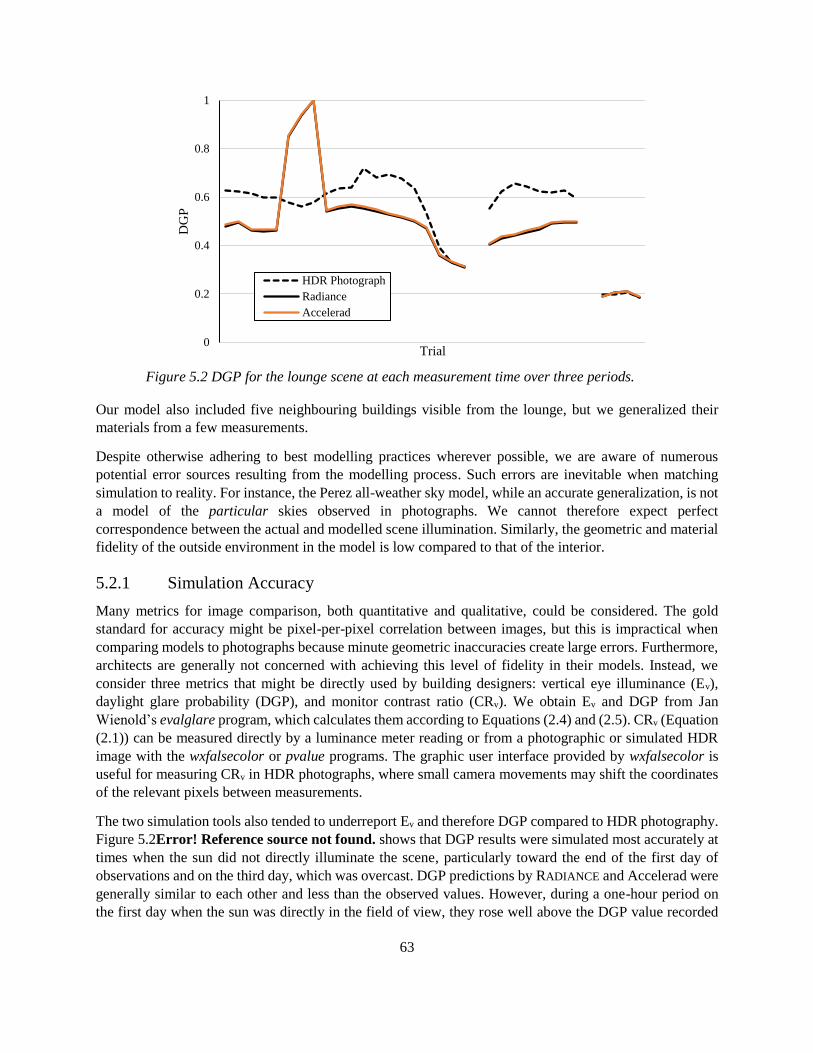
63

Our model also included five neighbouring buildings visible from the lounge, but we generalized their

materials from a few measurements.

Despite otherwise adhering to best modelling practices wherever possible, we are aware of numerous

potential error sources resulting from the modelling process. Such errors are inevitable when matching

simulation to reality. For instance, the Perez all-weather sky model, while an accurate generalization, is not

a model of the particular skies observed in photographs. We cannot therefore expect perfect

correspondence between the actual and modelled scene illumination. Similarly, the geometric and material

fidelity of the outside environment in the model is low compared to that of the interior.

5.2.1 Simulation Accuracy

Many metrics for image comparison, both quantitative and qualitative, could be considered. The gold

standard for accuracy might be pixel-per-pixel correlation between images, but this is impractical when

comparing models to photographs because minute geometric inaccuracies create large errors. Furthermore,

architects are generally not concerned with achieving this level of fidelity in their models. Instead, we

consider three metrics that might be directly used by building designers: vertical eye illuminance (Ev),

daylight glare probability (DGP), and monitor contrast ratio (CRv). We obtain Ev and DGP from Jan

Wienold’s evalglare program, which calculates them according to Equations (2.4) and (2.5). CRv (Equation

(2.1)) can be measured directly by a luminance meter reading or from a photographic or simulated HDR

image with the wxfalsecolor or pvalue programs. The graphic user interface provided by wxfalsecolor is

useful for measuring CRv in HDR photographs, where small camera movements may shift the coordinates

of the relevant pixels between measurements.

The two simulation tools also tended to underreport Ev and therefore DGP compared to HDR photography.

Figure 5.2Error! Reference source not found. shows that DGP results were simulated most accurately at

times when the sun did not directly illuminate the scene, particularly toward the end of the first day of

observations and on the third day, which was overcast. DGP predictions by RADIANCE and Accelerad were

generally similar to each other and less than the observed values. However, during a one-hour period on

the first day when the sun was directly in the field of view, they rose well above the DGP value recorded

Figure 5.2 DGP for the lounge scene at each measurement time over three periods.

0

0.2

0.4

0.6

0.8

1

DG

P

Trial

HDR Photograph

Radiance

Accelerad

64

by HDR photography. The low DGP in photographs resulted from luminous overflow, where light saturated

the camera’s sensor even at its shortest exposure [145]. Of the 29 unaffected values, Accelerad tended to

underpredict DGP by 0.101 (σ = 0.065), and RADIANCE underpredicted it by 0.106 (σ = 0.066).

There is close agreement on CRv between the two simulation engines and the two measurement techniques

(Figure 5.3). The simulations again tended to predict higher CRv values than were measured, but in this

case, the CRv values measured by the luminance meter were generally higher than those calculated from

HDR photographs. Accelerad’s results differed on average from the luminance meter by 0.14 (σ = 3.85)

and from HDR photography by 0.93 (σ = 1.50). RADIANCE’s results differed on average from the luminance

meter by 0.01 (σ = 3.78) and from HDR photography by 1.09 (σ = 1.52). While these errors are small, it is

worth noting that the actual CRv was frequently very close to CRmin, the minimum required by the current

ISO standard (Equation (2.2)). For scenes with lighting similar to ours, even small errors could result in

incorrect assessments of lighting quality.

Simulation times ranged from 13.1 to 16.8 minutes for Accelerad and from 341 to 378 minutes for

RADIANCE. The mean simulation time for Accelerad was 15.1 minutes (σ = 1.1 minutes), while for

RADIANCE it was 361 minutes (σ = 10.1 minutes). On average, Accelerad performed each simulation 24

times faster than RADIANCE (σ = 2.1).

5.2.2 Error Sources

RADIANCE and Accelerad have roughly equivalent accuracy for simulating the scene we tested. Both tools

tended to underpredict the total luminance of the scenes studied, and as a result, tended to overpredict CRv

and underpredict Ev and DGP. While the magnitude of error for visual comfort metrics was generally within

the accepted 20% bounds, the error is still sufficient to create problems in the use of visual comfort metrics.

The error in predicting CRv was small enough that it may be disregarded for practical applications.

However, in the lounge scene, the actual CRv was typically very close to the minimum allowable value.

The possibility that small numerical errors could lead to incorrect assessment of glare points to problems

with the enforceability of current standards.

Figure 5.3 CRv for the monitor in the lounge at each measurement time over three periods.

0

15

30

45

Mo

nit

or

Co

ntr

ast

Rat

io

Trial

Luminance Meter

HDR Photograph

Radiance

Accelerad

65

The error found in predicting DGP indicates a more serious problem with using this metric for the design

of daylit spaces. Accelerad’s underprediciton by 0.101 and RADIANCE’s underprediction by 0.106 are both

within the typical range of error seen in validations of daylighting simulation tools. However, as the

difference between imperceptible and intolerable glare is only 0.1 on this scale, we question whether today’s

best modelling practices provide useful glare predictions in cases that are “on the edge” of glare conditions.

The largest error found in this study was a systematic underpredicton of Ev by both simulation tools in

comparison to illuminance meter readings and HDR photography. Such systematic errors are generally the

result of discrepancies between the model and the real space. In this case, it could be the result of incorrect

source data from weather and IES files or of measurement errors in material reflectance and transmittance

data. In our second validation study, we aim to correct the errors that could have affected simulation

accuracy in our first study.

5.3 An Improved Validation Method

For our second study, we created a digital model of a real, sidelit space and compared photographically

obtained glare measurements from the space to values derived from RADIANCE and Accelerad simulations.

The space was a small conference room with a view to an enclosed courtyard in MIT’s Building 7. The

conference room measured 4.2 m × 3.9 m (13’5” × 12’9”) with a 3.2 m (10’7”) ceiling and a 2.1 m × 2.1 m

(7’7” × 7’7”) window facing west into the courtyard four floors above the ground, shown in Figure 5.4.

The courtyard measured approximately 86 m × 29 m (282’ × 95’) with the longer axis oriented roughly

north-to-south. Four and five-story buildings surrounded the courtyard on all sides. The entire building

complex was oriented at an angle of 24.25° to true compass directions such that the west-facing window

had a slightly southern exposure [146]. Conference room users reported that the space was prone to glare

conditions.

We furnished the conference room with a table and computer monitor in imitation of a workplace

environment. The monitor displayed a checkerboard test pattern and ran off a laptop hidden from view

beneath the table. We varied the orientation of the monitor from day to day as listed in Table 5.1 in order

to observe different glare conditions.

We compare HDR images of the space created through four levels of abstraction, as follows and shown in

Figure 5.5:

Photo: A photograph taken within the room.

Environment Map: A rendering of a digital model of the room in which a photograph of the view out

the window serves as an environmental luminance map.

Sky Map: A rendering of a digital model of the room and courtyard in which a photograph of the sky

serves as a sky luminance map.

Perez Model: A rendering of a digital model of the room and courtyard in which a modeled sky

provides luminance [132].

66

Figure 5.4 Top and side views of conference room model.

67

Figure 5.5 The four abstraction levels, with modeled geometry solid and photographed

geometry dashed.

The first abstraction, the photograph, serves as our reference, which we attempt to reproduce through

simulation with the others. The Perez model simulation is typical of simulations run by daylight analysts as

part of building design. However, while the Perez model yields the correct total illuminance based on

weather data, it does not necessarily provide the correct luminance distribution. The sky and environment

map simulations resolve this shortcoming of the Perez model using actual luminance distributions incident

on the building group and on the conference room window, respectively. We anticipated that this would

improve the accuracy of glare predictions over the Perez model’s ability.

5.4 Data Acquisition

We took measurements over a four-day period from April 12 – 15, 2016. April 12 was overcast with rain

early in the day and patchy skies by sunset. The remaining days had clear skies. Using a timer, the cameras

recorded images at five-minute intervals. In total, we captured image sets under 240 clear sky conditions

and 38 cloudy sky conditions. Table 5.1 lists measurement times and associated sky conditions. A dead

battery resulted in no data recorded during a 1.7-hour period on April 13.

Table 5.1 Observation periods and associated sky conditions

Date Time Interval Sky Condition Camera 1 Orientation

April 12 15:40 – 17:10 overcast

south 17:15 – 18:45 cloudy

April 13 09:35 – 14:20

clear south 16:05 – 18:35

April 14 12:50 – 17:30 clear east

April 15 10:05 – 17:50 clear west

68

5.4.1 Cameras

To record the luminous environment as described above, we placed cameras in the three locations shown

in Figure 5.6. The cameras were identical Canon EOS 5D Mark II full-frame cameras outfitted with Sigma

4.5mm F2.8 EX DC HSM Circular Fisheye lenses. Camera 1 was located inside the conference room facing

the monitor from a seated head height of 116 cm (46 inches). Camera 2 was placed on the windowsill facing

out to completely capture the view from the window. Camera 3 was placed on a roof adjacent to the

courtyard and oriented vertically to completely capture the sky dome. For protection against direct sunlight,

we outfitted cameras 2 and 3 with Neutral Density 3.0 Optical Gelatin Wratten 2 Filters between the camera

a b c

d e f

Figure 5.6 Cameras located (a) in the conference room, (b) on the windowsill, and (c) on

the roof, and (d, e, and f) their respective views.

69

body and lens. This strategy, proposed by Stumpfel, et al. [142], reduces the intensity of light passing

through the camera optics by a factor of 103.

To automate the timed capture of HDR photographs, we installed the Magic Lantern firmware add-on on

each camera [147]. We used exposure bracketing to capture a series of nine images on each push of the

shutter button, with exposure times ranging from 1/8000th to 4 seconds with the middle exposure being

1/60th second. This range includes the shortest possible shutter speed on the camera and also sufficiently

long exposures such that no pixels were underexposed in the 4-second exposure. We used the Magic

Lantern intervalometer option to trigger the shutter automatically at five-minute intervals. We set the white

balance setting to daylight, film speed to ISO-100, and f-stop to f/4 for each camera.

Converting the photographs to usable luminance maps required significant post-processing. We used the

program hdrgen by Gregory Ward to convert JPEG images from the camera to row-length encoded RGBE

HDR image files. For this, we used a response curve calculated for the camera that matched pixel brightness

to spot luminance measurements taken with a Konica Minolta LS-110 luminance meter. We performed

several additional calibration steps on the resulting HDR images. First, we cropped each image to a square

fit tightly around the fisheye view and black out the portion of this square outside the 180° circular fisheye

view. The exact cropping differed between cameras due to slight variation in lens alignment with the image

sensor and differences in focus adjustment. Second, we removed the vignette effect, which causes the edges

of the image to appear darker than the center, by applying the correction measured by Cauwerts, et al. [148]

for our camera, lens, and f-stop combination. Finally, we removed the geometric distortion created by the

lens to generate an equiangular projection in which distance from the center of the image is proportional to

angular displacement from the camera’s forward direction. This last step aimed to create precise alignment

between the photographs and equiangular RADIANCE renderings. However, lens optics do not create a single

central point from which angles can be measured. Instead, angles seen through the camera lens depend to

some extent on distance to the objects due to parallax, so our estimated geometric correction can be seen to

provide better alignment for near-field objects than for distant objects. Figure 5.7 and Figure 5.8 show

representative HDR photographs from overcast and clear days, respectively.

The cameras with neutral density filters also required an additional color-correction step. Contrary to their

name, neutral density filters are slightly spectrally selective and transmit roughly twice as much light in the

red and green bands as in blue. Stumpfel, et al. [142] estimate a color correction matrix but do not specify

their estimation method. We took HDR photographs of a Macbeth ColorChecker chart with and without

the neutral density filter under constant indoor lighting, and then computed a best-fit affine transformation

to map the RGB components of each chart square from the image with the filter to the image without [149].

Note that this transformation also accounts for the brightness scaling caused by the neutral density filter.

However, when used outdoors, HDR photographs produced with and without the neutral density filter still

differed in overall brightness by a factor of approximately 1.26, with the exact factor depending on the

color and brightness of the photographed object. In our tests, we apply this factor to images taken through

neutral density filters, but we acknowledge that the factor might depend on more fine-grained spectral data

than we are able to take into account. We see calibration of the neutral density filter as the largest potential

source of error in our study and a major hurdle for future studies.

5.4.2 Light Sources

We consider three light sources: the sky, sun, and computer monitor. We measured the luminance of white

and black pixels of the monitor directly with the Konica Minolta LS-110 luminance meter. To measure

70

combined direct and diffuse solar irradiation, we used an Onset® S-LIB-M003 silicon pyranometer

connected to a HOBO® weather station near camera 3.

On a clear day, the sun is brighter than the sky around it by several orders of magnitude, so incorporating

both into the same environment map would lead to significant undersampling of the sun. Instead, we

modeled the sun as a directional light source, as is customary in RADIANCE. For the Perez model, we split

a b

c d

Figure 5.7 The conference room on April 12 at 4:00pm under an overcast sky, shown in

(a) HDR photograph and rendered with (b) environment map simulation, (c) sky map

simulation, and (d) Perez model simulation.

3 3×1033×102 cd/m230

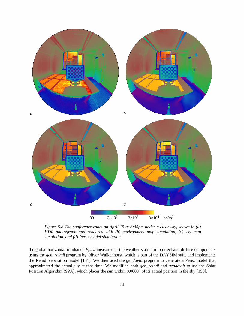
71

the global horizontal irradiance Eglobal measured at the weather station into direct and diffuse components

using the gen_reindl program by Oliver Walkenhorst, which is part of the DAYSIM suite and implements

the Reindl separation model [131]. We then used the gendaylit program to generate a Perez model that

approximated the actual sky at that time. We modified both gen_reindl and gendaylit to use the Solar

Position Algorithm (SPA), which places the sun within 0.0003° of its actual position in the sky [150].

a b

c d

Figure 5.8 The conference room on April 15 at 3:45pm under a clear sky, shown in (a)

HDR photograph and rendered with (b) environment map simulation, (c) sky map

simulation, and (d) Perez model simulation.

30 3×1043×103 cd/m23×102

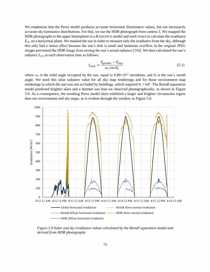
72

We emphasize that the Perez model produces accurate horizontal illuminance values, but not necessarily

accurate sky luminance distributions. For that, we use the HDR photograph from camera 3. We mapped the

HDR photographs to the upper hemisphere in a RADIANCE model and used rtrace to calculate the irradiance

Esky on a horizontal plane. We masked the sun in order to measure only the irradiance from the sky, although

this only had a minor effect because the sun’s disk is small and luminous overflow in the original JPEG

images prevented the HDR image from storing the sun’s actual radiance [143]. We then calculated the sun’s

radiance Lsun at each observation time as follows:

𝐿𝑠𝑢𝑛 =𝐸𝑔𝑙𝑜𝑏𝑎𝑙 − 𝐸𝑠𝑘𝑦

𝜔𝑠 cos 𝜃𝑠 (5.1)

where ωs is the solid angle occupied by the sun, equal to 6.80×10-5 steradians, and θs is the sun’s zenith

angle. We used this solar radiance value for all sky map renderings and for those environment map

renderings in which the sun was not occluded by buildings, which required θs < 64°. The Reindl separation

model predicted brighter skies and a dimmer sun than we observed photographically, as shown in Figure

5.9. As a consequence, the resulting Perez model skies exhibited a larger and brighter circumsolar region

than our environment and sky maps, as is evident through the window in Figure 5.8.

Figure 5.9 Solar and sky irradiance values calculated by the Reindl separation model and

derived from HDR photography.

0

100

200

300

400

500

600

700

800

900

1000

4/12 12 AM 4/12 12 PM 4/13 12 AM 4/13 12 PM 4/14 12 AM 4/14 12 PM 4/15 12 AM 4/15 12 PM 4/16 12 AM

Irra

dia

nce

(W

/m2)

Global horizontal irradiation Reindl direct normal irradiation

Reindl diffuse horizontal irradiation HDR direct normal irradiation

HDR diffuse horizontal irradiation

73

While the difference between the photographic and Perez model skies has a minor effect on the well-lit

scene in Figure 5.8, it is more pronounced under the overcast conditions in Figure 5.7. The Reindl separation

model accurately calculates that there was no direct solar component at the time of the photograph.

However, based on our calibration of the camera and neutral density filter, Esky is less than the measured

Eglobal, so the environment and sky map simulations incorrectly show direct sunlight entering the room. In

a separate study, Inanici and Hashemloo [151] introduced two corrections that could fix this error. First,

they did not use the neutral density filter at times when the solar corona was not visible. Second, they set a

1,000,000 cd/m2 threshold to determine whether the solar corona was visible, and otherwise ignore any

direct component and calibrate the HDR image brightness accordingly.

5.4.3 Geometry and Materials

We modeled the conference room and courtyard in SketchUp and exported it to the RADIANCE file format

using Thomas Bleicher’s su2rad plug-in. We attempted a high level of geometric detail in the conference

room model. We based our model of the courtyard on plans of the adjacent buildings. We used a Konica

Minolta CM-2500d spectrophotometer to measure the diffuse and specular reflectance of surfaces in the

conference room and courtyard. For each material, we took an average of three to six spectrophotometer

measurements, depending on the amount of color variation within the material. Post-processing of this data

allowed us to create custom RADIANCE materials for all opaque surfaces. We then estimated material

roughness to match appearance in our renderings. We determined the transmissivity of the glazed surfaces

with a Konica Minolta TL-1 illuminance meter. For three glass panes with a frosted coating adhered to

them, we also measured the fraction of directly transmitted light with the Konica Minolta LS-110 luminance

meter, which gives a very rough approximation of the amount of diffusion produced by the coating, and

otherwise used the model proposed by Reinhart and Andersen [111]. We catalogued and measured 55

materials, of which we show the more common materials in Table 5.2.

5.4.4 Display Monitor

Monitor screens must be modeled with accurate reflective properties in order to predict CRv. A liquid-

crystal display (LCD) monitor has two main components: a luminous panel (typically lit by LEDs around

its perimeter) and a liquid crystal layer sandwiched between sheets of polarized plastic or glass. Applying

a voltage across a region of the liquid crystal layer causes that region to become transparent. A bidirectional

reflectance distribution function (BRDF) measured by a goniophotometer can produce realistic simulated

reflections [152]. In the absence of such equipment and given that BRDFs are not commonly published for

LCD screens, the sandwich layer can be modeled as a translucent panel with parameters derived using

Reinhart and Andersen’s [111] model. This, however, requires the monitor be disassembled to measure the

diffuse and specular transmittance across the sandwich layer. We opted to estimate screen material

properties without altering the monitor.

We modelled the monitor screen as RADIANCE glow materials positioned behind RADIANCE trans materials

(Figure 5.10). Using diffuse and specular reflectance values measured with the spectrophotometer as input,

we selected a transmissivity value that allowed the sandwich layer to transmit light without significantly

altering its reflective properties according to Reinhart and Andersen’s [111] model. The selected value is

low, which makes sense because we measured the screen’s reflectance in its off state. While the reflectance

characteristics could be different in the activated clear state, we lacked the ability to measure this and instead

assume constant characteristics for the transparent layer, listed in Table 5.2. We scaled the glow intensities

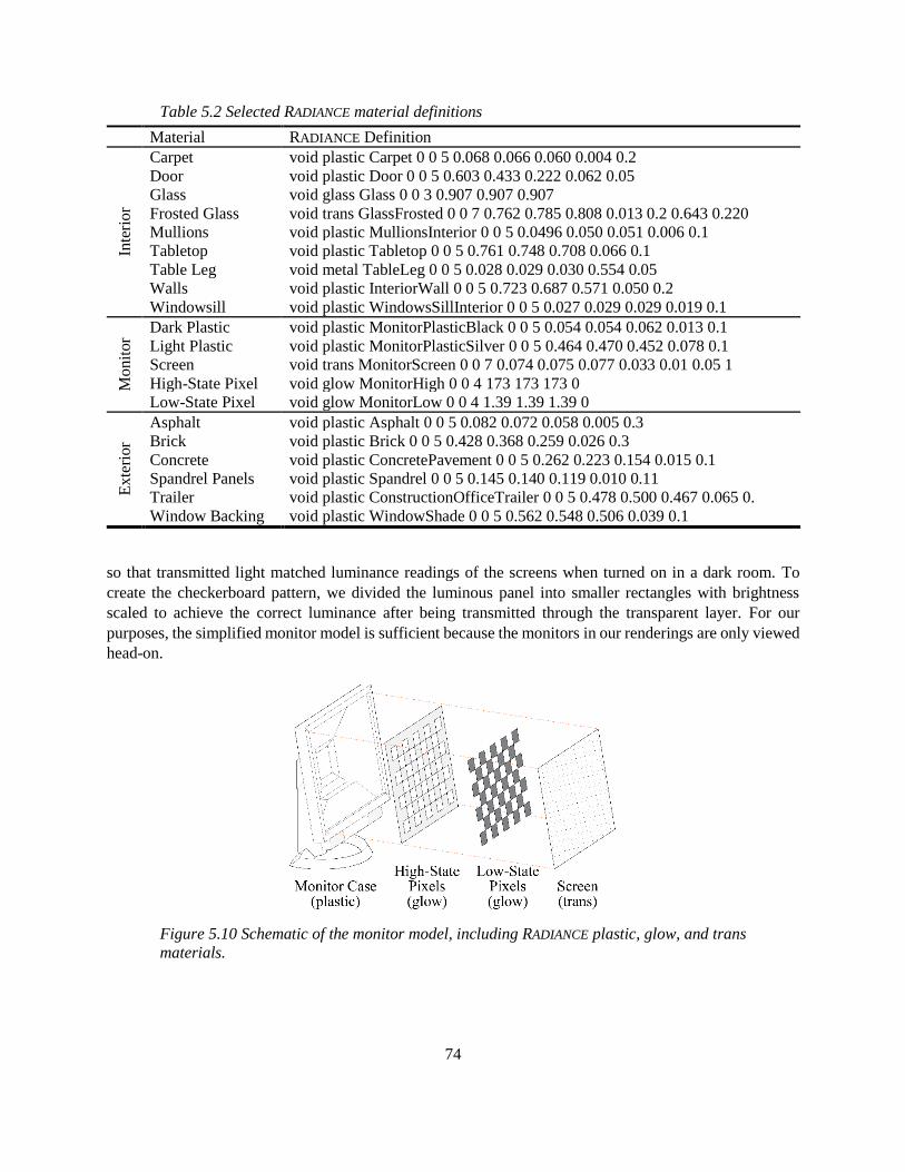
74

so that transmitted light matched luminance readings of the screens when turned on in a dark room. To

create the checkerboard pattern, we divided the luminous panel into smaller rectangles with brightness

scaled to achieve the correct luminance after being transmitted through the transparent layer. For our

purposes, the simplified monitor model is sufficient because the monitors in our renderings are only viewed

head-on.

Figure 5.10 Schematic of the monitor model, including RADIANCE plastic, glow, and trans

materials.

Table 5.2 Selected RADIANCE material definitions

Material RADIANCE Definition In

teri

or

Carpet void plastic Carpet 0 0 5 0.068 0.066 0.060 0.004 0.2

Door void plastic Door 0 0 5 0.603 0.433 0.222 0.062 0.05

Glass void glass Glass 0 0 3 0.907 0.907 0.907

Frosted Glass void trans GlassFrosted 0 0 7 0.762 0.785 0.808 0.013 0.2 0.643 0.220

Mullions void plastic MullionsInterior 0 0 5 0.0496 0.050 0.051 0.006 0.1

Tabletop void plastic Tabletop 0 0 5 0.761 0.748 0.708 0.066 0.1

Table Leg void metal TableLeg 0 0 5 0.028 0.029 0.030 0.554 0.05

Walls void plastic InteriorWall 0 0 5 0.723 0.687 0.571 0.050 0.2

Windowsill void plastic WindowsSillInterior 0 0 5 0.027 0.029 0.029 0.019 0.1

Mo

nit

or

Dark Plastic void plastic MonitorPlasticBlack 0 0 5 0.054 0.054 0.062 0.013 0.1

Light Plastic void plastic MonitorPlasticSilver 0 0 5 0.464 0.470 0.452 0.078 0.1

Screen void trans MonitorScreen 0 0 7 0.074 0.075 0.077 0.033 0.01 0.05 1

High-State Pixel void glow MonitorHigh 0 0 4 173 173 173 0

Low-State Pixel void glow MonitorLow 0 0 4 1.39 1.39 1.39 0

Exte

rior

Asphalt void plastic Asphalt 0 0 5 0.082 0.072 0.058 0.005 0.3

Brick void plastic Brick 0 0 5 0.428 0.368 0.259 0.026 0.3

Concrete void plastic ConcretePavement 0 0 5 0.262 0.223 0.154 0.015 0.1

Spandrel Panels void plastic Spandrel 0 0 5 0.145 0.140 0.119 0.010 0.11

Trailer void plastic ConstructionOfficeTrailer 0 0 5 0.478 0.500 0.467 0.065 0.

Window Backing void plastic WindowShade 0 0 5 0.562 0.548 0.506 0.039 0.1

75

5.5 Simulations

We used RADIANCE rpict version 5.0.11 to render the luminous environment in our conference room model

to 512 × 512 pixel images using the environment map, sky map, and Perez models as luminance sources.

We repeated these simulations in Accelerad rpict. The Accelerad version was equivalent to the classic

RADIANCE version, except that it performed ray tracing in parallel on the GPU and implemented a pre-

computed irradiance cache by means of adaptive sampling and k-means clustering [128]. Both classic

RADIANCE and Accelerad use stochastic algorithms. In order to remove potential random bias from our

results, we repeated each simulation eight times and report the median value of each metric across the eight

trials.

5.5.1 Comparison Metrics

We considered both luminance metrics and luminance-based visual discomfort metrics in assessing the

accuracy of our predictive rendering. We used the images from camera 1 as a baseline for all comparisons.

We compared luminance using global and local metrics. For global comparison, we used Jan Wienold’s

evalglare program to calculate Ev for each image in Equation (2.4). The error in Ev is most directly

comparable to errors reported in previous studies based on illuminance sensors, which also integrate over

a visible hemisphere.

However, two images with different luminance distributions may produce the same Ev. For local

comparison, we could measure error pixel-by-pixel using mean bias error and root mean square error, but

such a comparison will be highly influenced by small geometric misalignments between high-contrast

objects. Various solutions have been proposed to counter the effect of misalignment, such as using average

luminance values across grids [100], Tregenza patches [133], and task areas [83]. We opt for the latter

method and compare luminance values for image regions relevant to visual discomfort. For each region R,

the average luminance is:

𝐿𝑅 =∑ 𝐿𝑝𝜔𝑝∀𝑝∈𝑅

∑ 𝜔𝑝∀𝑝∈𝑅 (5.2)

We then compute the relative error ηR at that region:

𝜂𝑅 =𝐿𝑅,𝐻𝐷𝑅 − 𝐿𝑅,𝑠𝑖𝑚𝑢𝑙𝑎𝑡𝑖𝑜𝑛

𝐿𝑅,𝐻𝐷𝑅 (5.3)

From there, we can compute MBErel across n images as follows:

MBErel =1

𝑛∑𝜂𝑅,𝑖

𝑛

𝑖=1

(5.4)

We calculate relative rather than absolute errors because they allow better comparison across times and

studies. Absolute error values scale with light source intensity, which changed constantly during our tests.

Similarly, we considered both global and local visual discomfort metrics. For a global metric, we used DGP

calculated by evalglare as shown in Equation 4. For local contrast, we extend Equations (2.1) and (2.3) to

CRv and CRd, to consider pixel regions as follows:

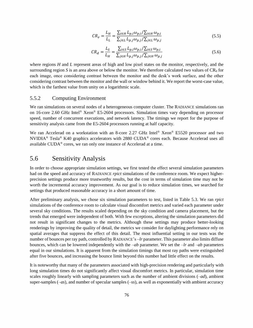
76

𝐶𝑅𝑣 =𝐿𝐻

𝐿𝐿=

∑ 𝐿𝑝,𝑖𝜔𝑝,𝑖𝑖∈𝐻 ∑ 𝜔𝑝,𝑖𝑖∈𝐻⁄

∑ 𝐿𝑝,𝑗𝜔𝑝,𝑗𝑗∈𝐿 ∑ 𝜔𝑝,𝑗𝑗∈𝐿⁄ (5.5)

𝐶𝑅𝑑 =𝐿𝑆

𝐿𝐻=

∑ 𝐿𝑝,𝑖𝜔𝑝,𝑖𝑖∈𝑆 ∑ 𝜔𝑝,𝑖𝑖∈𝑆⁄

∑ 𝐿𝑝,𝑗𝜔𝑝,𝑗𝑗∈𝐻 ∑ 𝜔𝑝,𝑗𝑗∈𝐻⁄ (5.6)

where regions H and L represent areas of high and low pixel states on the monitor, respectively, and the

surrounding region S is an area above or below the monitor. We therefore calculated two values of CRd for

each image, once considering contrast between the monitor and the desk’s work surface, and the other

considering contrast between the monitor and the wall or window behind it. We report the worst-case value,

which is the farthest value from unity on a logarithmic scale.

5.5.2 Computing Environment

We ran simulations on several nodes of a heterogeneous computer cluster. The RADIANCE simulations ran

on 16-core 2.60 GHz Intel® Xeon® E5-2604 processors. Simulation times vary depending on processor

speed, number of concurrent executions, and network latency. The timings we report for the purpose of

sensitivity analysis came from the E5-2604 processors running at half capacity.

We ran Accelerad on a workstation with an 8-core 2.27 GHz Intel® Xeon® E5520 processor and two

NVIDIA® Tesla® K40 graphics accelerators with 2880 CUDA® cores each. Because Accelerad uses all

available CUDA® cores, we ran only one instance of Accelerad at a time.

5.6 Sensitivity Analysis

In order to choose appropriate simulation settings, we first tested the effect several simulation parameters

had on the speed and accuracy of RADIANCE rpict simulations of the conference room. We expect higher-

precision settings produce more trustworthy results, but the cost in terms of simulation time may not be

worth the incremental accuracy improvement. As our goal is to reduce simulation times, we searched for

settings that produced reasonable accuracy in a short amount of time.

After preliminary analysis, we chose six simulation parameters to test, listed in Table 5.3. We ran rpict

simulations of the conference room to calculate visual discomfort metrics and varied each parameter under

several sky conditions. The results scaled depending on the sky condition and camera placement, but the

trends that emerged were independent of both. With few exceptions, altering the simulation parameters did

not result in significant changes to the metrics. Although these settings may produce better-looking

renderings by improving the quality of detail, the metrics we consider for daylighting performance rely on

spatial averages that suppress the effect of this detail. The most influential setting in our tests was the

number of bounces per ray path, controlled by RADIANCE’s –lr parameter. This parameter also limits diffuse

bounces, which can be lowered independently with the –ab parameter. We set the –lr and –ab parameters

equal in our simulations. It is apparent from the simulation timings that most ray paths were extinguished

after five bounces, and increasing the bounce limit beyond this number had little effect on the results.

It is noteworthy that many of the parameters associated with high-precision rendering and particularly with

long simulation times do not significantly affect visual discomfort metrics. In particular, simulation time

scales roughly linearly with sampling parameters such as the number of ambient divisions (–ad), ambient

super-samples (–as), and number of specular samples (–ss), as well as exponentially with ambient accuracy

77

(–aa) and minimum ray weight (–lw). However, for the investigated space, varying these parameters did

not produce significant differences in visual discomfort predictions.

As a representative example, we show Ev at 4:30pm on April 13 in Figure 5.11, based on the median results

of eight trials for each parameter combination. Using these results as a guide, we chose simulation parameter

values not to produce the best-looking image, but rather to produce visual discomfort predictions with

roughly the same accuracy as the best renderings in less time. We list the ultimately chosen settings in bold

in Table 5.3. Figure 5.7 and Figure 5.8 show representative renderings created with the chosen parameters.

While rendering artifacts are readily apparent in these images, those artifacts are random and localized, so

they are unlikely to bias visual discomfort predictions.

5.7 Accuracy Analysis

In our second experiment, we compared HDR images from four abstraction levels to determine how well

each predicted glare in the conference room. We chose the first abstraction level, the HDR photograph, as

a reference because the DGP metric was developed for photographs [83]. For each of the remaining

abstraction levels, we ran simulations in RADIANCE rpict and Accelerad rpict. For RADIANCE, we ran an

overture pass to populate an irradiance cache stored in an ambient file followed by a final pass to produce

the finished rendering. Accelerad builds its irradiance cache prior to rendering, so no overture pass was

necessary. We ran eight simulations for each recorded sky condition with each engine and recorded the

median results to eliminate random error. The standard deviation among Ev and DGP results within each

group of eight simulations was always one to two orders of magnitude smaller than the mean value, leading

us to conclude that random error was not a significant factor for global metrics. However, the standard

deviation among dark regions such as the low-state pixel region and back wall calculated by RADIANCE

could be as high at 15% or 20%, respectively. As a result, contrast-based metrics from separate runs can

disagree on the presence or absence of glare when the contrast ratio is near its limit.

Table 5.3 RADIANCE simulation parameters

Parameter Argument Values

Varied

Ambient accuracy –aa 0.05, 0.10, 0.15, 0.20, 0.25

Ambient divisions –ad 64, 256, 512, 1024, 2048, 4096

Ambient super-samples –as 0, 1, 2, 20, 50, 512

Ray reflection limit –lr, –ab 0, 1, 2, 3, 4, 5, 6, 7, 8

Ray weight limit –lw 2e-3, 1e-3, 5e-4, 2e-4, 1e-4, 5e-5, 2e-5, 1e-5, 5e-6, 2e-6, 1e-6

Specular samples –ss 0, 0.5, 1, 16, 32, 64, 1024

Constant

Ambient resolution –ar 96 (12 for environment map due to smaller scene dimensions)

Ambient value –av r = 0, g = 0, b = 0

Direct certainty –dc 0

Direct jitter –dj 0

Direct sampling –ds 0.01

Direct threshold –dt 0

Direct relays –dr 3

Specular threshold –st 0.01

Pixel sampling –ps 1

Image size –x, –y 512

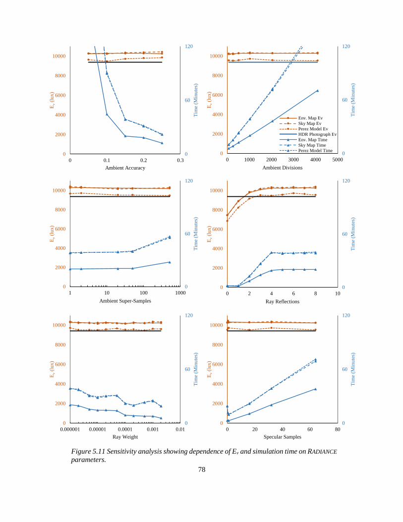
78

Figure 5.11 Sensitivity analysis showing dependence of Ev and simulation time on RADIANCE

parameters.

0

60

120

0

2000

4000

6000

8000

10000

0 0.1 0.2 0.3

Tim

e (M

inu

tes)

Ev

(lu

x)

Ambient Accuracy

0

60

120

0

2000

4000

6000

8000

10000

0 1000 2000 3000 4000 5000

Tim

e (M

inu

tes)

Ev

(lu

x)

Ambient Divisions

Env. Map Ev

Sky Map Ev

Perez Model Ev

HDR Photograph Ev

Env. Map Time

Sky Map Time

Perez Model Time

0

60

120

0

2000

4000

6000

8000

10000

1 10 100 1000

Tim

e (M

inu

tes)

Ev

(lu

x)

Ambient Super-Samples

0

60

120

0

2000

4000

6000

8000

10000

0 2 4 6 8 10

Tim

e (M

inu

tes)

Ev

(lu

x)

Ray Reflections

0

60

120

0

2000

4000

6000

8000

10000

0.000001 0.00001 0.0001 0.001 0.01

Tim

e (M

inu

tes)

Ev

(lu

x)

Ray Weight

0

60

120

0

2000

4000

6000

8000

10000

0 20 40 60 80

Tim

e (M

inu

tes)

Ev

(lu

x)

Specular Samples

79

Environment Map Sky Map Perez Model

Ap

ril

12

4:0

0pm

A

pri

l 1

3

2:0

0pm

Apri

l 1

3

4:3

0pm

Apri

l 14

2:0

0pm

Apri

l 14

4:0

0pm

Apri

l 15

2:0

0pm

Ap

ril

15

4:0

0pm

<-2500 cd/m2 >2500 cd/m2

Figure 5.12 Difference images between RADIANCE simulations and HDR photographs,

with simulation excess luminance in red and simulation deficit luminance in blue.

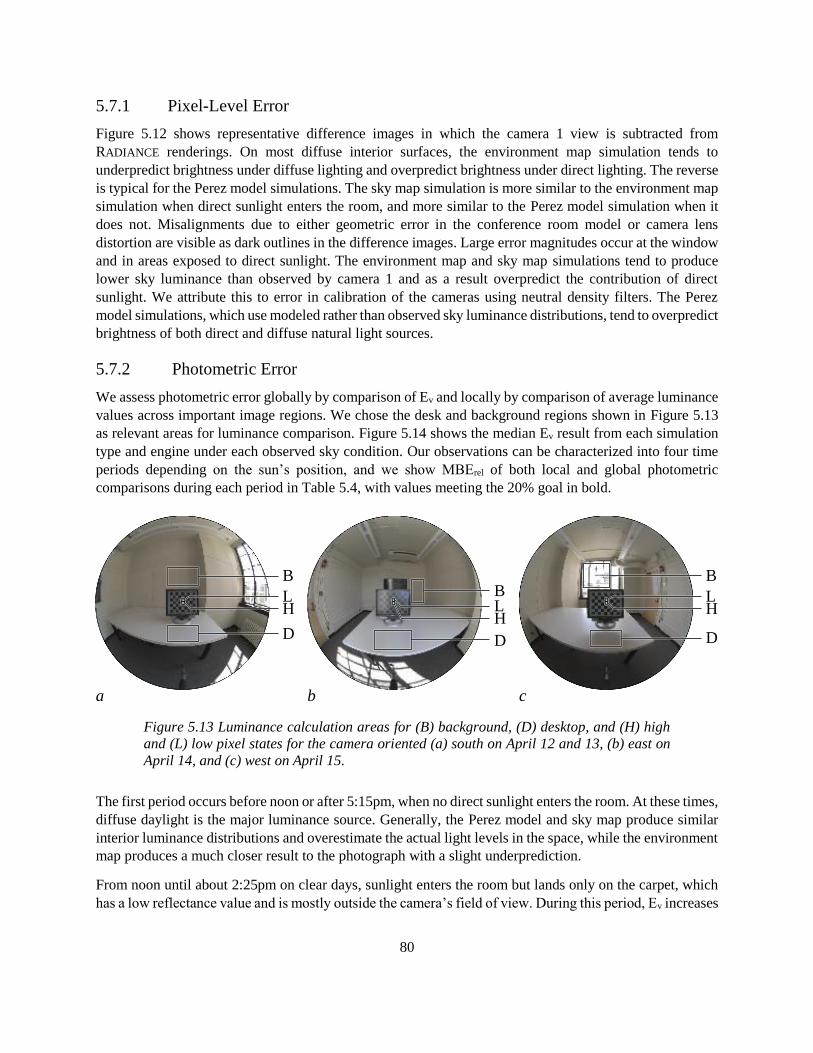
80

5.7.1 Pixel-Level Error

Figure 5.12 shows representative difference images in which the camera 1 view is subtracted from

RADIANCE renderings. On most diffuse interior surfaces, the environment map simulation tends to

underpredict brightness under diffuse lighting and overpredict brightness under direct lighting. The reverse

is typical for the Perez model simulations. The sky map simulation is more similar to the environment map

simulation when direct sunlight enters the room, and more similar to the Perez model simulation when it

does not. Misalignments due to either geometric error in the conference room model or camera lens

distortion are visible as dark outlines in the difference images. Large error magnitudes occur at the window

and in areas exposed to direct sunlight. The environment map and sky map simulations tend to produce

lower sky luminance than observed by camera 1 and as a result overpredict the contribution of direct

sunlight. We attribute this to error in calibration of the cameras using neutral density filters. The Perez

model simulations, which use modeled rather than observed sky luminance distributions, tend to overpredict

brightness of both direct and diffuse natural light sources.

5.7.2 Photometric Error

We assess photometric error globally by comparison of Ev and locally by comparison of average luminance

values across important image regions. We chose the desk and background regions shown in Figure 5.13

as relevant areas for luminance comparison. Figure 5.14 shows the median Ev result from each simulation

type and engine under each observed sky condition. Our observations can be characterized into four time

periods depending on the sun’s position, and we show MBErel of both local and global photometric

comparisons during each period in Table 5.4, with values meeting the 20% goal in bold.

Figure 5.13 Luminance calculation areas for (B) background, (D) desktop, and (H) high

and (L) low pixel states for the camera oriented (a) south on April 12 and 13, (b) east on

April 14, and (c) west on April 15.

The first period occurs before noon or after 5:15pm, when no direct sunlight enters the room. At these times,

diffuse daylight is the major luminance source. Generally, the Perez model and sky map produce similar

interior luminance distributions and overestimate the actual light levels in the space, while the environment

map produces a much closer result to the photograph with a slight underprediction.

From noon until about 2:25pm on clear days, sunlight enters the room but lands only on the carpet, which

has a low reflectance value and is mostly outside the camera’s field of view. During this period, Ev increases

a b

B

LH

D

BLH

D

B

LH

D

c

81

steadily. As the amount of direct sunlight entering the room increases, the behavior of the sky map

simulations diverges from the Perez model and becomes more similar to the environment map. In some

cases, the sky map also underpredicts Ev.

During the period from 2:30pm until 4:55pm on clear days, sunlight falls directly on the white table surface,

causing a dramatic increase in Ev. All three simulation methods tend to overpredict Ev as a result of

overestimating the direct solar contribution to global horizontal irradiance; this trend is more pronounced

for the sky map and environment map, which have larger direct solar components. However, when the view

faces the window, the visible area of the sky has a countering effect that reduces or negates the

overprediction of Ev.

Between 5:00pm and 5:15pm, the sun sets behind the building opposite the courtyard. As the building’s

shadow moves across the window, Ev diminishes back to the levels noted in the first period. The Perez

Figure 5.14 Photographic measurements and simulation predictions of Ev by RADIANCE

and Accelerad.

0

5000

10000

15000

15:00 16:00 17:00 18:00 19:00

Ev

(lux)

April 12

HDR Photo

Radiance Env.

Radiance Sky

Radiance Perez

Accelerad Env.

Accelerad Sky

Accelerad Perez

0

5000

10000

15000

9:00 11:00 13:00 15:00 17:00 19:00

Ev

(lux)

April 13

0

5000

10000

15000

12:00 13:00 14:00 15:00 16:00 17:00 18:00

Ev

(lux)

April 14

0

5000

10000

15000

9:00 11:00 13:00 15:00 17:00 19:00

Ev

(lux)

April 15

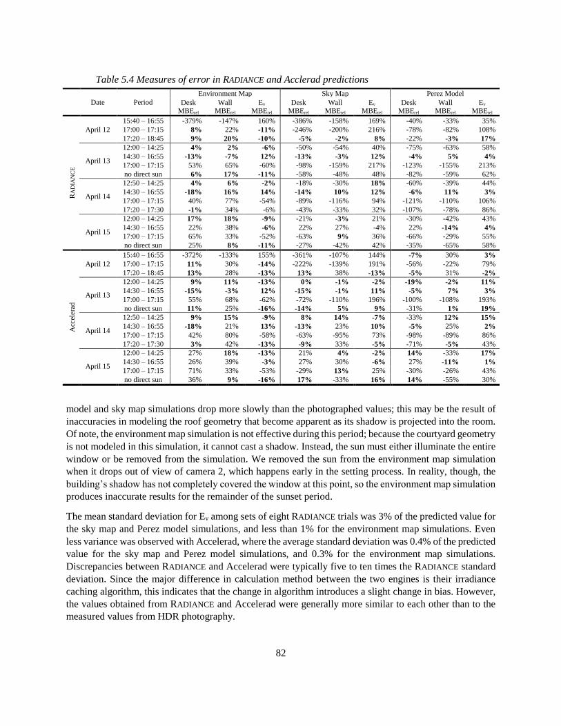
82

model and sky map simulations drop more slowly than the photographed values; this may be the result of

inaccuracies in modeling the roof geometry that become apparent as its shadow is projected into the room.

Of note, the environment map simulation is not effective during this period; because the courtyard geometry

is not modeled in this simulation, it cannot cast a shadow. Instead, the sun must either illuminate the entire

window or be removed from the simulation. We removed the sun from the environment map simulation

when it drops out of view of camera 2, which happens early in the setting process. In reality, though, the

building’s shadow has not completely covered the window at this point, so the environment map simulation

produces inaccurate results for the remainder of the sunset period.

The mean standard deviation for Ev among sets of eight RADIANCE trials was 3% of the predicted value for

the sky map and Perez model simulations, and less than 1% for the environment map simulations. Even

less variance was observed with Accelerad, where the average standard deviation was 0.4% of the predicted

value for the sky map and Perez model simulations, and 0.3% for the environment map simulations.

Discrepancies between RADIANCE and Accelerad were typically five to ten times the RADIANCE standard

deviation. Since the major difference in calculation method between the two engines is their irradiance

caching algorithm, this indicates that the change in algorithm introduces a slight change in bias. However,

the values obtained from RADIANCE and Accelerad were generally more similar to each other than to the

measured values from HDR photography.

Table 5.4 Measures of error in RADIANCE and Acclerad predictions

Date Period


Desk MBErel

Wall MBErel

Ev MBErel

Desk MBErel

Wall MBErel

Ev MBErel

Desk MBErel

Wall MBErel

Ev MBErel

RA

DIA

NC

E

April 12

15:40 – 16:55 -379% -147% 160% -386% -158% 169% -40% -33% 35%

17:00 – 17:15 8% 22% -11% -246% -200% 216% -78% -82% 108%

17:20 – 18:45 9% 20% -10% -5% -2% 8% -22% -3% 17%

April 13

12:00 – 14:25 4% 2% -6% -50% -54% 40% -75% -63% 58%

14:30 – 16:55 -13% -7% 12% -13% -3% 12% -4% 5% 4%

17:00 – 17:15 53% 65% -60% -98% -159% 217% -123% -155% 213%

no direct sun 6% 17% -11% -58% -48% 48% -82% -59% 62%

April 14

12:50 – 14:25 4% 6% -2% -18% -30% 18% -60% -39% 44%

14:30 – 16:55 -18% 16% 14% -14% 10% 12% -6% 11% 3%

17:00 – 17:15 40% 77% -54% -89% -116% 94% -121% -110% 106%

17:20 – 17:30 -1% 34% -6% -43% -33% 32% -107% -78% 86%

April 15

12:00 – 14:25 17% 18% -9% -21% -3% 21% -30% -42% 43%

14:30 – 16:55 22% 38% -6% 22% 27% -4% 22% -14% 4%

17:00 – 17:15 65% 33% -52% -63% 9% 36% -66% -29% 55%

no direct sun 25% 8% -11% -27% -42% 42% -35% -65% 58%

Acc

eler

ad

April 12

15:40 – 16:55 -372% -133% 155% -361% -107% 144% -7% 30% 3%

17:00 – 17:15 11% 30% -14% -222% -139% 191% -56% -22% 79%

17:20 – 18:45 13% 28% -13% 13% 38% -13% -5% 31% -2%

April 13

12:00 – 14:25 9% 11% -13% 0% -1% -2% -19% -2% 11%

14:30 – 16:55 -15% -3% 12% -15% -1% 11% -5% 7% 3%

17:00 – 17:15 55% 68% -62% -72% -110% 196% -100% -108% 193%

no direct sun 11% 25% -16% -14% 5% 9% -31% 1% 19%

April 14

12:50 – 14:25 9% 15% -9% 8% 14% -7% -33% 12% 15%

14:30 – 16:55 -18% 21% 13% -13% 23% 10% -5% 25% 2%

17:00 – 17:15 42% 80% -58% -63% -95% 73% -98% -89% 86%

17:20 – 17:30 3% 42% -13% -9% 33% -5% -71% -5% 43%

April 15

12:00 – 14:25 27% 18% -13% 21% 4% -2% 14% -33% 17%

14:30 – 16:55 26% 39% -3% 27% 30% -6% 27% -11% 1%

17:00 – 17:15 71% 33% -53% -29% 13% 25% -30% -26% 43%

no direct sun 36% 9% -16% 17% -33% 16% 14% -55% 30%

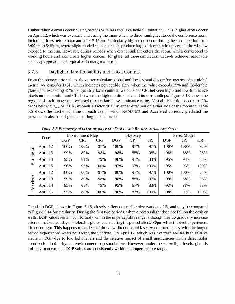
83

Higher relative errors occur during periods with less total available illumination. Thus, higher errors occur

on April 12, which was overcast, and during the times when no direct sunlight entered the conference room,

including times before noon and after 5:15pm. Particularly high errors occur during the sunset period from

5:00pm to 5:15pm, where slight modeling inaccuracies produce large differences in the area of the window

exposed to the sun. However, during periods when direct sunlight enters the room, which correspond to

working hours and also create higher concern for glare, all three simulation methods achieve reasonable

accuracy approaching a typical 20% margin of error.

5.7.3 Daylight Glare Probability and Local Contrast

From the photometric values above, we calculate global and local visual discomfort metrics. As a global

metric, we consider DGP, which indicates perceptible glare when the value exceeds 35% and intolerable

glare upon exceeding 45%. To quantify local contrast, we consider CRv between high- and low-luminance

pixels on the monitor and CRd between the high monitor state and its surroundings. Figure 5.13 shows the

regions of each image that we used to calculate these luminance ratios. Visual discomfort occurs if CRv

drops below CRmin or if CRd exceeds a factor of 10 in either direction on either side of the monitor. Table

5.5 shows the fraction of time on each day in which RADIANCE and Accelerad correctly predicted the

presence or absence of glare according to each metric.

Table 5.5 Frequency of accurate glare prediction with RADIANCE and Accelerad

Date Environment Map Sky Map Perez Model

DGP CRv CRd DGP CRv CRd DGP CRv CRd

RA

DIA

NC

E April 12 100% 100% 97% 100% 97% 97% 100% 100% 92%

April 13 99% 89% 98% 98% 88% 98% 98% 88% 98%

April 14 95% 81% 79% 98% 91% 83% 95% 93% 83%

April 15 96% 92% 100% 97% 92% 100% 95% 93% 100%

Acc

eler

ad April 12 100% 100% 97% 100% 97% 97% 100% 100% 71%

April 13 99% 89% 98% 98% 88% 97% 99% 88% 98%

April 14 95% 65% 79% 95% 67% 83% 93% 88% 83%

April 15 95% 88% 100% 96% 87% 100% 98% 92% 100%

Trends in DGP, shown in Figure 5.15, closely reflect our earlier observations of Ev and may be compared

to Figure 5.14 for similarity. During the first two periods, when direct sunlight does not fall on the desk or

walls, DGP values remain comfortably within the imperceptible range, although they do gradually increase

after noon. On clear days, intolerable glare occurs during the period after 2:30pm when the desk experiences

direct sunlight. This happens regardless of the view direction and lasts two to three hours, with the longer

period experienced when not facing the window. On April 12, which was overcast, we see high relative

errors in DGP due to low light levels and the relative impact of small inaccuracies in the direct solar

contribution in the sky and environment map simulations. However, under these low light levels, glare is

unlikely to occur, and DGP values are consistently within the imperceptible range.

84

Figure 5.15 Photographic measurements and simulation predictions of DGP by RADIANCE

and Accelerad.

Veiling glare due to low CRv occurred when sunlight fell directly on the monitor, even at glancing angles.

On April 14, when the monitor was oriented facing the window, photographed reflections on the monitor

were so strong that some low-luminance pixels appeared brighter than their high-luminance neighbors,

completely veiling the checkerboard pattern. A few instances in which veiling glare is not detected during

this timeframe are actually false negatives occurring when the shadow of a mullion overlaps a low-

luminance square of the checkerboard. In general, the environment map simulations predict higher CRv

than the other simulations. Simulations tended to overpredict CRv when the monitor faced the window, and

underpredict CRv when the monitor was oriented in other directions. This frequent underprediction

indicates that our method for estimating the monitor screen’s material parameters yielded too-high

reflectance values. Figure 5.16 shows CRv measurements from camera 1 and predictions from the three

simulation methods.

0

0.2

0.4

0.6

0.8

1

15:00 16:00 17:00 18:00 19:00

DG

PApril 12

HDR Photo

Radiance Env.

Radiance Sky

Radiance Perez

Accelerad Env.

Accelerad Sky

Accelerad Perez

0

0.2

0.4

0.6

0.8

1

9:00 11:00 13:00 15:00 17:00 19:00

DG

P

April 13

0

0.2

0.4

0.6

0.8

1

12:00 13:00 14:00 15:00 16:00 17:00 18:00

DG

P

April 14

0

0.2

0.4

0.6

0.8

1

9:00 11:00 13:00 15:00 17:00 19:00

DG

P

April 15

85

Figure 5.16 Photographic measurements and simulation predictions of CRv by RADIANCE

and Accelerad.

Accelerad tended to predict higher CRv than RADIANCE. This brought the Accelerad predictions closer to

the observed values on April 12 and 13, when simulations tended to underpredict CRv, and farther from

observation on April 14 and 15, when simulations overpredicted CRv. This is reflected in the rates at which

RADIANCE and Accelerad predicted veiling glare according to the ISO standard, as visible in Table 5.5.

Discomfort and disability glare also occur due to extreme CRd when the background illuminance is ten

times greater than the monitor’s luminance. This happens when direct sunlight falls on the desk or the wall

behind the monitor. This type of glare is a constant problem when the monitor sits in front of the window

as on April 15. On the overcast day, the reverse occurs where the monitor is more than ten times brighter

than the wall behind it in some Perez model simulations. We measured CRd with respect to both the desk

and back wall and present whichever value was farther from unity on a log scale, which causes CRd to

appear discontinuous, especially on April 12 and 14. Figure 5.17 shows CRd measurements from camera 1

and predictions from the three simulation methods, which we summarize in Table 5.5.

1

3

9

27

81

15:00 16:00 17:00 18:00 19:00

CR

vApril 12

1

3

9

27

81

9:00 11:00 13:00 15:00 17:00 19:00

CR

v

April 13

1

3

9

27

81

12:00 13:00 14:00 15:00 16:00 17:00 18:00

CR

v

April 14

HDR Photo

Radiance Env.

Radiance Sky

Radiance Perez

Accelerad Env.

Accelerad Sky

Accelerad Perez

1

3

9

27

81

9:00 11:00 13:00 15:00 17:00 19:00

CR

v

April 15

86

Figure 5.17 Photographic measurements and simulation predictions of CRd by RADIANCE

and Accelerad.

For the most part, the CRv and CRd metrics predict glare during the same periods in which DGP is greater

than 35%, which rates as either perceptible or intolerable glare, as we show in a timeline in Figure 5.18.

The major exception occurs on April 15, when the monitor was oriented in front of the window, in which

case there is significant contrast between the monitor and the brighter window, as seen in the high CRd

values. This prompts the question of whether CRd is an appropriate glare metric, as it lacks a basis in

research and is considered too stringent by some [74]. We suggest that discomfort and disability glare can

be adequately addressed using the DGP metric alone.

5.8 Speed Analysis

A precise statement about the speedup achieved by using the GPU through Accelerad is difficult and

perhaps not meaningful because of the heterogeneous computing environment. The environment map

simulations ran faster because they involved fewer surfaces and skipped the calculation of irradiance values

0.01

0.1

1

10

100

15:00 16:00 17:00 18:00 19:00

CR

dApril 12

0.01

0.1

1

10

100

9:00 11:00 13:00 15:00 17:00 19:00

CR

d

April 13

0.01

0.1

1

10

100

12:00 13:00 14:00 15:00 16:00 17:00 18:00

CR

d

April 14

0.01

0.1

1

10

100

9:00 11:00 13:00 15:00 17:00 19:00

CR

d

April 15

HDR Photo

Radiance Env.

Radiance Sky

Radiance Perez

Accelerad Env.

Accelerad Sky

Accelerad Perez

87

for the outdoor part of the scene. Sky map and Perez model simulations tended to take the same amount of

time, and both ran faster for later simulations when the cluster’s workload decreased. Early simulations,

which occupied all available cores, each took nearly twice as long as later simulations, which used

approximately 75% of available cores. We do not present average timings here, as they depend heavily on

processor speed and would be heavily influenced by changing the number of concurrent executions.

However, we do present the range of simulation times in Table 5.6, from which one can get a sense of the

times. Note that even though Accelerad ran on the computer with the slowest central processor, the

availability of GPU accelerators made it the fastest engine. Accelerad achieved speedups ranging from 16

to 44 times faster than RADIANCE. Figure 5.19 shows average timings for each set of eight simulation runs.

Table 5.6 Range of elapsed simulation times based on 2384 simulations per method


RADIANCE Accelerad RADIANCE Accelerad RADIANCE Accelerad

Fastest Time (minutes) 24.84 1.20 30.19 1.31 30.34 1.31

Slowest Time (minutes) 32.09 1.68 66.13 1.89 65.67 1.90

5.9 Recommendations

To our knowledge, this study is the first systematic validation of RADIANCE and Accelerad as tools for

image-based visual discomfort prediction. We used both engines to calculate photometric (luminance and

illuminance) and discomfort (glare and contrast) metrics and compared the results to values obtained from

HDR photographs. The accuracy of our photometric predictions was on par with those of previous

RADIANCE validation studies. While we did not consistently achieve accuracy within the 20% margin of

error expected in simulations today, we have already noted other studies that encountered similar

difficulties. When it comes to the simple question of whether or not glare occurs at a given time, we fare

much better. We predicted the DGP glare classification with between 93% and 99% accuracy, depending

on the camera’s orientation, and discomfort glare due to contrast with between 71% and 99% accuracy.

Veiling glare was more difficult to predict in some cases due to a monitor screen model that did not

accurately duplicate observed reflections.

Figure 5.18 Timeline of periods of glare observed and predicted by each simulation type.

15 10 11 12 13 14 15 16 17 13 14 15 16 1718 11 12 13 14 15 16 1716 17

HDR Photograph

Acc

eler

adR

AD

IAN

CE

DGPNo Glare Glare

April 12 April 13 April 14 April 15

CRv

CRdEnv. Map

Sky Map

Perez Model

Env. Map

Sky Map

Perez Model

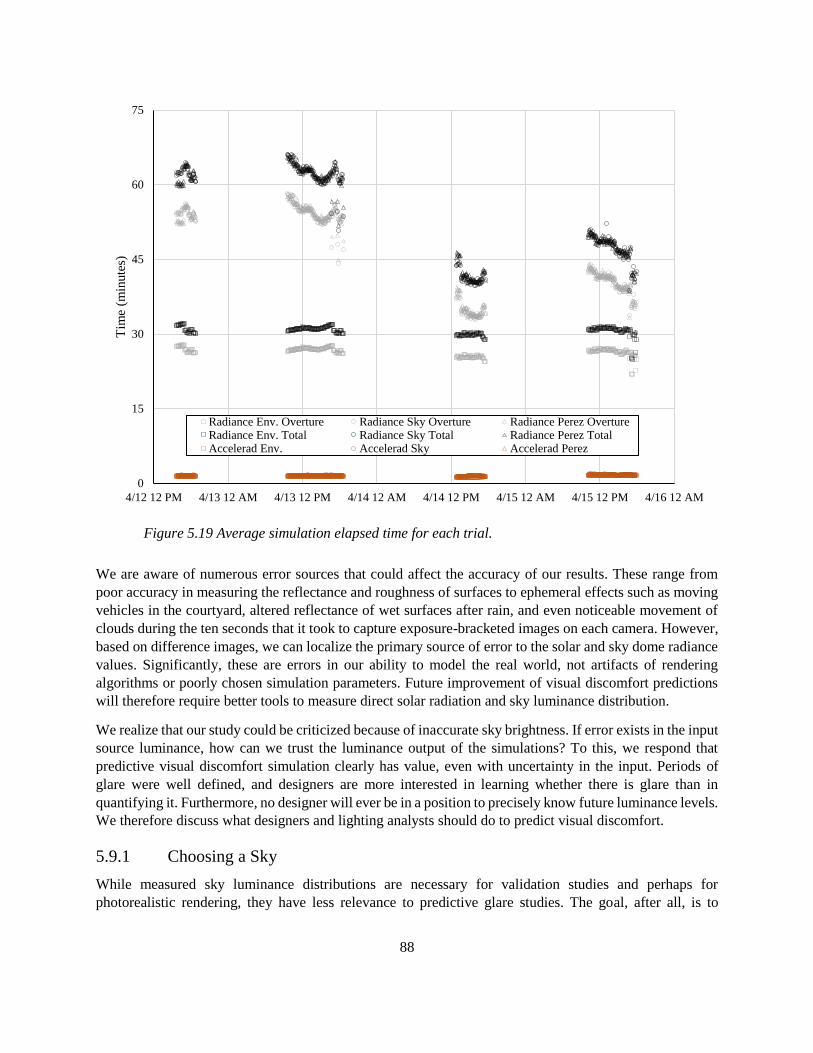
88

Figure 5.19 Average simulation elapsed time for each trial.

We are aware of numerous error sources that could affect the accuracy of our results. These range from

poor accuracy in measuring the reflectance and roughness of surfaces to ephemeral effects such as moving

vehicles in the courtyard, altered reflectance of wet surfaces after rain, and even noticeable movement of

clouds during the ten seconds that it took to capture exposure-bracketed images on each camera. However,

based on difference images, we can localize the primary source of error to the solar and sky dome radiance

values. Significantly, these are errors in our ability to model the real world, not artifacts of rendering

algorithms or poorly chosen simulation parameters. Future improvement of visual discomfort predictions

will therefore require better tools to measure direct solar radiation and sky luminance distribution.

We realize that our study could be criticized because of inaccurate sky brightness. If error exists in the input

source luminance, how can we trust the luminance output of the simulations? To this, we respond that

predictive visual discomfort simulation clearly has value, even with uncertainty in the input. Periods of

glare were well defined, and designers are more interested in learning whether there is glare than in

quantifying it. Furthermore, no designer will ever be in a position to precisely know future luminance levels.

We therefore discuss what designers and lighting analysts should do to predict visual discomfort.

5.9.1 Choosing a Sky

While measured sky luminance distributions are necessary for validation studies and perhaps for

photorealistic rendering, they have less relevance to predictive glare studies. The goal, after all, is to

0

15

30

45

60

75

4/12 12 PM 4/13 12 AM 4/13 12 PM 4/14 12 AM 4/14 12 PM 4/15 12 AM 4/15 12 PM 4/16 12 AM

Tim

e (m

inute

s)

Radiance Env. Overture Radiance Sky Overture Radiance Perez OvertureRadiance Env. Total Radiance Sky Total Radiance Perez TotalAccelerad Env. Accelerad Sky Accelerad Perez

89

anticipate future conditions, not to match past conditions. Most of the visual discomfort issues we observed

were caused by excessive luminance from the sun and sky. Therefore, simulation with a generic clear sky

is likely to yield the worst-case situations that designers need to consider. This is good news for practice

because synthetic clear skies can be created by well-established workflows.

Our analysis suggests that HDR sky and environment maps do not necessarily produce better predictions

of visual discomfort than smooth Perez models of sky luminance distribution. Although the sky and

environment maps successfully capture luminance distribution patterns, scaling them to provide real

photometric values is difficult, especially when using neutral density filters. Furthermore, any error in

scaling rolls over into calculation of the direct solar component. We do not rule out that future work could

produce correctly scaled sky luminance distribution maps from photographs; in fact, this could lead to major

improvements over mathematically modeled skies. Doing so will likely require integration over narrow

wavelength bands to accurately convert between photometric and radiometric units.

5.9.2 Choosing Simulation Parameters

In practice, we have observed a trend toward higher precision simulation parameters, and therefore longer

running simulations, in order to calculate DGP and other RADIANCE-based metrics. This is likely due to the

prevalent notion that renderings must be free of artifacts in order to provide useful building performance

results. High-precision simulation settings that eliminate rendering artifacts certainly contribute to the

impression of photorealism in renderings, but this study shows that we can reliably derive visual discomfort

metrics from images that one would generally not consider useful for architectural representation.

Designers should understand which simulation parameters affect biased errors, and therefore rendering

accuracy, and which parameters affect random errors, and therefore rendering precision. To predict visual

discomfort or luminance values over broad regions, we can reduce simulation time by choosing parameters

with high accuracy and low precision. The number of ray bounces, controlled by the RADIANCE’s –lr and

–ab parameters, should be high enough that no important ray paths from the eye terminate before reaching

a source. We find values of 5 or 6 to be sufficient, although higher settings might be required for detailed

simulation of complex fenestration systems. Other parameters including ambient divisions (–ad), ambient

super-samples (–as), number of specular samples (–ss), and minimum ray weight (–lw) had little effect on

our results, and we recommend the bolded settings in Table 5.3.

The ambient accuracy (–aa) parameter deserves special attention, as it can affect both precision and

accuracy and has a large effect on simulation run times. We took two steps to minimize the bias introduced

by this parameter. First, we prevented light leaks by enclosing our conference room model in a box made

of non-reflective material that we added to RADIANCE’s ambient exclude list. We cut a hole in this box for

the window, leaving that as the single portal for rays to exit the conference room model. Second, we set the

ambient resolution (–ar) parameter to ignore variation in diffuse lighting intensities at scales much smaller

than our analysis regions. RADIANCE defines this cut-off by a minimum ambient radius rmin in terms of the

maximum scene dimension dmax and the –aa and –ar parameters as follows:

𝑟𝑚𝑖𝑛 = 𝑑𝑚𝑎𝑥

𝑎𝑎

𝑎𝑟 (5.7)

In our more precise simulations with ambient accuracy set to 0.05, we chose an ambient resolution so as to

set rmin to 5 cm (2 in.), although we found an ambient accuracy of 0.15 to provide sufficient accuracy, which

put rmin at 15 cm (6 in.).

90

5.9.3 Choosing Simulation Tools

In order to achieve improved building performance, simulation tools must be able to provide results on

demand to building designers. In our study, Accelerad produced comparable results to RADIANCE, and did

so 16 – 44 times faster. In fact, the Accelerad simulations, which average between 1.2 and 1.9 minutes in

run time, represent a speedup over one hundred times faster than many high-precision glare analysis

simulations we see in practice today.

However, the past decade has seen the release of many new physically based simulation tools that, although

they have received little treatment in scientific validation studies, still satisfy physically based rendering’s

energy-balance equation. In particular, we will show in Chapter 7 that progressive path tracing can provide

visual discomfort estimates in a matter of seconds rather than minutes. It is worthwhile for the building

performance simulation community to evaluate new, parallel, and scalable rendering engines.

5.10 Summary

Fast ray tracing simulations that calculate DGP are an effective way to predict and mitigate glare when

designing buildings. Simulations can also predict veiling glare by calculating CRv, but monitor models must

have accurate reflection characteristics. We recorded visual discomfort conditions in a conference room

over four days using HDR photography and reproduced them using several predictive rendering

approaches. RADIANCE and Accelerad produced similar predictions in all cases, though Accelerad ran

between 16 and 44 times faster in our computing environment. Although we tried to use HDR photography

of the sky to produce a more accurate source luminance distribution, the Perez model most often gave the

best agreement with interior measured values. We expect that HDR photography would have produced

more accurate sky luminance distributions if our cameras had been better calibrated, but calculating direct

normal irradiance based on our HDR sky photography and global horizontal irradiance proved difficult.

However, the use of an environment map based on HDR photography taken from the windowsill led to

faster RADIANCE simulation times and produced reasonably accurate results without the need to model the

outdoor environment so long as outside objects did not shade the window.

Errors in our study stemmed mainly from modeling inaccuracies, particularly the difficulty of determining

source luminance distribution from the sky and of representing complex materials such as the monitor

screen. In comparison, the error introduced by using fairly low-precision simulation parameters is minimal.

Fast simulations should be sufficient to predict visual discomfort in buildings without complex fenestration

systems, and these simulations can be made even faster with GPU acceleration. We note the need to repeat

this type of sensitivity analysis for spaces with complex fenestration systems that direct light into a space

through many bounces or by specular reflection.

Most importantly, we found that reasonably accurate tools and workflows are already available to the

building design community, and that fast simulation settings and adoption of recently developed rendering

tools can further speed up simulations. The ability to produce fast and reliable predictions of luminance and

visual discomfort is an important step toward integrating simulation directly into design practice. In our

final chapters, we will turn to making annual simulation and glare prediction faster and more accessible to

architects, which will allow increased planning of and sensitivity to visual comfort.

91

6 Annual Simulation

In this chapter, we turn our attention from image rendering, which is specific to a point in time and space,

to climate-based daylighting metrics (CBDMs), which quantify annual daylighting for entire spaces. The

chapter combines work from two studies. The first study, Fast daylight coefficient calculation using

graphics hardware, was published in 2015 [16]. It describes an Accelerad version of rtrace_dc, the core

ray-tracing program of DAYSIM. The second study, Speedup potential of climate-based daylight modelling

on GPUs, will be published this year [17]. It describes an Accelerad version of rcontrib, the ray-tracing

program used in the three-phase method [18] and five-phase method [19]. Using a model of a generic office,

we achieve speedups of twenty-five times with the five-phase method and ten times with DAYSIM. Parallel

implementations of three- and five-phase methods provide better scaling to multi-GPU environments and

more accurate results for complex fenestration systems than parallelized DAYSIM. Finally, we comment

on limitations of GPU-based methods with respect to daylight coefficient calculation and on future work

that may overcome these limitations.

6.1 Calculating Climate-Based Daylighting Metrics

As humans spend 90 percent of the time inside of buildings, the need to provide natural lighting to indoor

spaces is becoming widely recognized [153]. However, defining, and therefore predicting, good daylighting

is far from a straightforward task. While many lighting simulation tools lend themselves to point-in-time

calculations, building performance metrics must take into account the annual performance of the building,

which requires simulation under multiple solar positions and sky conditions. Climate-based daylighting

metrics (CBDMs) represent the annual daylighting performance of a space, an abstract quantity that agrees

closely with subjective occupant observations [5]. While CBDMs are useful from a building standards

standpoint, their computation is slow and requires more memory than older illuminance-based metrics,

making them difficult to integrate into design tools. Serial CBDM calculations are prohibitively time-

consuming during early design stages when the designs change rapidly. In order to produce CBDM results

at interactive rates to feed back into an iterative design process, we must use new methods and platforms

to calculate them.

If we assume that a typical office is occupied for eight hours each day, or 2920 hours per year, then a naïve

approach to calculating CBDMs would be to run 2920 point-in-time daylighting simulations over a grid of

sensors with RADIANCE’s rtrace program, once for each hour. On each iteration, rtrace would trace rays

from each sensor through the scene along multiple-bounce paths until reaching the sun and sky and

sampling the brightness of each. However, every simulation would trace the same ray paths and differ only

by the brightness of the sky where the rays reach it. This approach results in considerable duplicated work

and programmatic inefficiency.

DAYSIM and the three- and five-phase methods all avoid duplicating work by using the ray-tracing step to

calculate matrix entries. The matrix (or product of matrices) is a transformation function between source

radiance and sensor irradiance values. When multiplied by a vector containing a given sky condition, it

produces an array of sensor values. Although the details of the methods differ, as we will describe later,

both DAYSIM’s rtrace_dc and the three- and five-phase methods’ rcontrib are simple modifications of the

original rtrace algorithm.

92

6.1.1 DAYSIM

In DAYSIM, the matrix entries are daylight coefficients. Each daylight coefficient represents the

contribution of a light source to a sensor, such that the total illuminance at that point is the sum of all direct

and diffuse daylight coefficients multiplied by the respective luminance values of their sources at a

particular point in time [154]. Daylight coefficients are calculated using distribution ray tracing [8]; starting

from a grid of points at which daylight autonomies are to be calculated, rays are traced through a user-

defined number of bounces until a source is encountered. The simulation can be made more accurate (and

slower) by increasing the number of bounces through the –ab parameter or increasing the ambient accuracy

by decreasing the –aa parameter.

DAYSIM calculates direct and diffuse daylight coefficients separately (with rtrace_dc), creating two

matrices and then concatenating them (with gen_dc). For the diffuse matrix Ddif, DAYSIM uses 148 sources

corresponding to the 145 Tregenza sky divisions [133] and three ring-shaped ground patches. For the direct

matrix Ddir, DAYSIM creates directional sources spaced uniformly along the solar paths of the chosen

latitude [9]. The number of direct daylight coefficients varies by latitude; 63 are needed at Boston’s location.

The final step (carried out by ds_illum) is to calculate the irradiance matrix I listing the irradiance at each

sensor for each time of the year as follows:

𝐼 = 𝐷𝑑𝑖𝑟𝑆𝑠𝑢𝑛 + 𝐷𝑑𝑖𝑓𝑆𝑠𝑘𝑦 = (𝐷𝑑𝑖𝑟|𝐷𝑑𝑖𝑓)(𝑆𝑠𝑢𝑛|𝑆𝑠𝑘𝑦) (6.1)

where the matrices Ssun and Ssky list the radiance of each sun position and sky patch, respectively, at each

hour of the year. In practice, the values reported from DAYSIM have units of illuminance (lux) rather than

irradiance (W/m2), which is achieved by multiplying I by 179 lm/W [71].

DAYSIM is frequently accessed through the graphic user interface of DIVA-for-Rhino [155]. DAYSIM

computes daylight coefficients, representing the illuminance contributions of the sun and sky, which can in

turn be used to compute the daylight autonomy of a space [9]. Like the RADIANCE suite of programs on

which it is based [114], DAYSIM uses serial ray tracing to perform lighting calculations.

6.1.2 Three- and Five-Phase Methods

The three-phase method may be understood as an evolution from DAYSIM. It differs in two key ways.

First, the brightness of the sun is added to the sky dome to create a single sky matrix S (calculated by

gendaymtx). This eliminates the need for separate direct and diffuse ray tracing passes but also removes

hard shadows. Second, the daylight coefficient matrix is replaced with a product of three matrices

(calculated by rcontrib). These are the daylight matrix D, relating light that reaches windows to its sources

in the sky, the transmission matrix T, which is a bidirectional scattering distribution function (BSDF) that

describes light passing through a window or complex fenestration system in terms of light incident on that

surface, and the view matrix V, relating light leaving a window to the light arriving at sensors. The entries

in each matrix are no longer daylight coefficients, since they do not describe the complete source-to-sensor

relationship, so instead we call them contribution coefficients. The irradiance matrix is calculated (by

dctimestep) as:

𝐼 = 𝑉𝑇𝐷𝑆 (6.2)

Unlike rtrace_dc, rcontrib performs separate calculations in the red, green, and blue channels and

interleaves them in the matrices. We convert the results to illuminance as follows:

93

𝐿 = 179 × (0.2651𝑟 + 0.670𝑔 + 0.065𝑏) (6.3)

where L is illuminance in lux and r, g, and b are the red, green, and blue irradiance values in W/m2 [71].

The five-phase method extends the three-phase method by separating the direct irradiance calculation. This

makes it possible to render hard shadows and otherwise brings the method in line with the standard daylight

coefficient model proposed by Bourgeois, et al. [156]. After running a normal three-phase method

simulation, the next step is to isolate and remove the direct contribution from the previously calculated

result. This means repeating the calculation of D and V with no light bounces (using a non-reflective, black

version of the model) to determine how much light must be removed. These direct-only matrices Dd and

Vd, are used together with a direct sun-only sky matrix Sds. Finally, the direct sun component is added back

in using a fine grid of suns centered in Reinhart sky patches, which are subdivisions of Tregenza sky patches

[156]. The use of the Reinhart sky patches stored in Ssun allows simulation results to be reused for multiple

building orientations or geographic locations, although this flexibility is more useful in academic study than

in practice. The calculation again uses a non-reflective, black model, with the exception of windows, which

retain their transparency, and the calculation produces actual daylight coefficients in Cds instead of

contribution coefficients because BSDFs are not relevant to direct ray paths. The entire five-phase method

is then:

𝐼 = 𝑉𝑇𝐷𝑆 − 𝑉𝑑𝑇𝐷𝑑𝑆𝑑𝑠 + 𝐶𝑑𝑠𝑆𝑠𝑢𝑛 (6.4)

6.1.3 Validation

CBDM calculation methods derive from rtrace, so we expect they should also achieve accuracy within our

20% goal. This expectation is borne out through a number of studies of DAYSIM. Several studies

comparing daylit interiors to DAYSIM predictions found relative mean bias error (MBErel) under 20% and

relative root mean square error (RMSErel) under 32% [9, 111]. DAYSIM gave comparable results to 3ds

Max in a study of one building interior under a number of sky conditions [110] but offered superior results

at four other geographic locations [23].

Validation of the three- and five-phase methods shows similar accuracy. The three-phase method produced

close agreement with theoretical flux values for venetian blinds [18] and had MBErel less than 13% and

RMSErel less than 23% for a light-redirecting component [157]. In a study of four classrooms, the three-

and five-phase methods gave similar sDA300,50% results to each other and to DAYSIM, although more

variance occurred in ASE1000,250 [158]. Images created with the three- and five-phase methods had similar

appearance to conventional RADIANCE rpict images and produced similar image-based predictions of

daylight glare probability [151].

6.2 Implementation

Before we describe our modifications to parallelize rtrace_dc and rcontrib for the GPU, it is useful to cover

some core concepts of ray tracing. Here, we present a brief primer on ray tracing and the programs involved

in DAYSIM and the three- and five-phase methods.

DAYSIM is a collection of programs often called through interfaces such as DIVA-for-Rhino. DAYSIM

prepares daylight coefficients through three calls to gen_dc, the first two to initiate calculation of diffuse

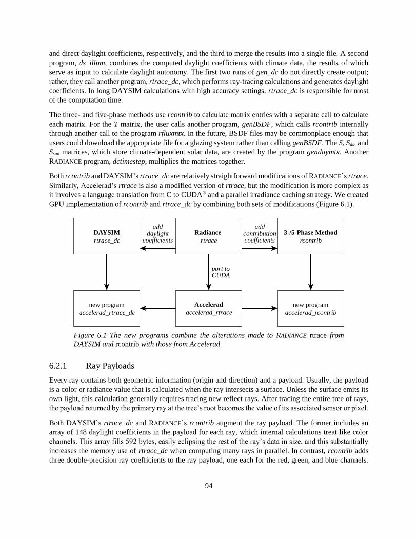
94

and direct daylight coefficients, respectively, and the third to merge the results into a single file. A second

program, ds_illum, combines the computed daylight coefficients with climate data, the results of which

serve as input to calculate daylight autonomy. The first two runs of gen_dc do not directly create output;

rather, they call another program, rtrace_dc, which performs ray-tracing calculations and generates daylight

coefficients. In long DAYSIM calculations with high accuracy settings, rtrace_dc is responsible for most

of the computation time.

The three- and five-phase methods use rcontrib to calculate matrix entries with a separate call to calculate

each matrix. For the T matrix, the user calls another program, genBSDF, which calls rcontrib internally

through another call to the program rfluxmtx. In the future, BSDF files may be commonplace enough that

users could download the appropriate file for a glazing system rather than calling genBSDF. The S, Sds, and

Ssun matrices, which store climate-dependent solar data, are created by the program gendaymtx. Another

RADIANCE program, dctimestep, multiplies the matrices together.

Both rcontrib and DAYSIM’s rtrace_dc are relatively straightforward modifications of RADIANCE’s rtrace.

Similarly, Accelerad’s rtrace is also a modified version of rtrace, but the modification is more complex as

it involves a language translation from C to CUDA® and a parallel irradiance caching strategy. We created

GPU implementation of rcontrib and rtrace_dc by combining both sets of modifications (Figure 6.1).

Figure 6.1 The new programs combine the alterations made to RADIANCE rtrace from

DAYSIM and rcontrib with those from Accelerad.

6.2.1 Ray Payloads

Every ray contains both geometric information (origin and direction) and a payload. Usually, the payload

is a color or radiance value that is calculated when the ray intersects a surface. Unless the surface emits its

own light, this calculation generally requires tracing new reflect rays. After tracing the entire tree of rays,

the payload returned by the primary ray at the tree’s root becomes the value of its associated sensor or pixel.

Both DAYSIM’s rtrace_dc and RADIANCE’s rcontrib augment the ray payload. The former includes an

array of 148 daylight coefficients in the payload for each ray, which internal calculations treat like color

channels. This array fills 592 bytes, easily eclipsing the rest of the ray’s data in size, and this substantially

increases the memory use of rtrace_dc when computing many rays in parallel. In contrast, rcontrib adds

three double-precision ray coefficients to the ray payload, one each for the red, green, and blue channels.

Radiance

rtrace

addcontributioncoefficients

port toCUDA

3-/5-Phase Method

rcontrib

Accelerad

accelerad_rtrace

new program

accelerad_rcontrib

adddaylight

coefficients

DAYSIM

rtrace_dc

new program

accelerad_rtrace_dc

95

The cost per ray for the additional payload is only 24 bytes. Rather than accumulating value, as a color or

daylight coefficient payload would, ray coefficients represent the weighting factor of each color channel in

calculating that channel’s value for the parent ray. When a ray hits a surface or source with a material of

interest specified by the user (usually a light source), rcontrib adds the cumulative product of the ray

coefficients in the current tree to a contribution coefficient for that material. At the conclusion of ray tracing,

the program outputs the coefficients rather than the radiance values. Any lighting condition produced by a

set of sources (or sky patches) is a linear combination of the contribution coefficients.

Because rcontrib calculates coefficients at leaf nodes of the ray tree rather than at the root, as DAYSIM

does, it is incompatible with irradiance caching. However, irradiance caching artificially increases the

sampling importance of diffuse rays far from the root. Without it, the minimum ray weight would need to

be set extremely low to simulate diffuse lighting accurately, which would severely increase simulation

times. To avoid this, the three- and five-phase methods advise the use of Russian roulette, which terminates

rays at random beyond a certain depth in the tree, and the remaining rays receive accordingly higher weights

[93]. The rcontrib program enables Russian roulette by default.

6.2.2 Global Memory Use

Memory limitations are an important consideration in porting code to the GPU. While today’s GPUs have

large global memory spaces (12 GB for our devices), little local memory is available to each thread. In

OptiX™, each thread is limited to 256 registers, which is not enough space to store even a single daylight

coefficient array; the remainder must spill into global memory where it cannot be accessed as quickly.

6.2.2.1 Memory in rtrace_dc

We can reduce, though not eliminate, this inefficiency in rtrace_dc by allocating space for daylight

coefficient storage in GPU global memory prior to starting the simulation. The strategy is to create a buffer

in the GPU’s global memory with dimensions x × y × z, where x and y are taken from the –x and –y

arguments and z is based on the maximum number of reflections given by the –lr argument as follows:

𝑧 = 2𝐷𝐶 × (1 + 𝑙𝑟) (6.5)

where DC is the size of the array of daylight coefficients in bytes. This reserves one daylight coefficient

array to store the cumulative daylight coefficients for each ray until tracing of that ray is complete and

another daylight coefficient array for intermediate calculations at each hit, which is needed for ambient and

Gaussian specular computations (Figure 6.2). Each GPU thread accesses only the daylight coefficient arrays

belonging to one (x, y) pair. Under this scheme, a DAYSIM simulation of a 10×10 sensor grid with 148

single-precision daylight coefficients and a maximum of 8 ray reflections requires about a megabyte of

GPU global memory, which is well within the limits of today’s GPUs. Ambient calculations require

additional memory depending on the number of irradiance cache entries.

Each ray payload and hit calculation stores an index to a daylight coefficient in global memory, rather than

an entire set of daylight coefficients. The index, stored as an integer x-y-z triplet, requires 12 bytes and fits

easily in the GPU thread’s local memory. This also means that details of the implementation, such as the

number and size of daylight coefficients, can be changed without affecting local memory requirements. For

instance, while our current implementation copies DAYSIM’s use of a single color channel for daylight

coefficients, future implementations could store separate daylight coefficients in red, green, and blue

channels without increasing local memory requirements.

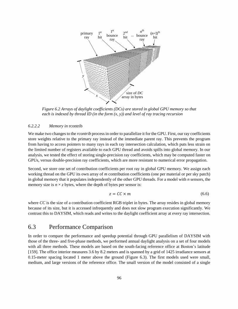
96

Figure 6.2 Arrays of daylight coefficients (DCs) are stored in global GPU memory so that

each is indexed by thread ID (in the form (x, y)) and level of ray tracing recursion

6.2.2.2 Memory in rcontrib

We make two changes to the rcontrib process in order to parallelize it for the GPU. First, our ray coefficients

store weights relative to the primary ray instead of the immediate parent ray. This prevents the program

from having to access pointers to many rays in each ray intersection calculation, which puts less strain on

the limited number of registers available to each GPU thread and avoids spills into global memory. In our

analysis, we tested the effect of storing single-precision ray coefficients, which may be computed faster on

GPUs, versus double-precision ray coefficients, which are more resistant to numerical error propagation.

Second, we store one set of contribution coefficients per root ray in global GPU memory. We assign each

working thread on the GPU its own array of m contribution coefficients (one per material or per sky patch)

in global memory that it populates independently of the other GPU threads. For a model with n sensors, the

memory size is n × z bytes, where the depth of bytes per sensor is:

𝑧 = 𝐶𝐶 × 𝑚 (6.6)

where CC is the size of a contribution coefficient RGB triplet in bytes. The array resides in global memory

because of its size, but it is accessed infrequently and does not slow program execution significantly. We

contrast this to DAYSIM, which reads and writes to the daylight coefficient array at every ray intersection.

6.3 Performance Comparison

In order to compare the performance and speedup potential through GPU parallelism of DAYSIM with

those of the three- and five-phase methods, we performed annual daylight analysis on a set of four models

with all three methods. These models are based on the south-facing reference office at Boston’s latitude

[159]. The office interior measures 3.6 by 8.2 meters and is spanned by a grid of 1425 irradiance sensors at

0.15-meter spacing located 1 meter above the ground (Figure 6.3). The first models used were small,

medium, and large versions of the reference office. The small version of the model consisted of a single

x

y

size of DCarray in bytes

primaryray

1st

hit

1st

bounceray

nth

bounceray

2nd

hit... (n+1)th

hit

97

reference office, while the medium and large models consisted of two and ten side-by-side copies of the

office yielding 2850 and 14250 sensors, respectively. We define model size in terms of the number of

sensors because this quantity directly affects simulation time. The modularity of our models also forces

DAYSIM’s irradiance cache to grow proportionally with model size rather than treating it as a separate

variable. The fourth model was the same as the first with the addition of exterior blinds.

Figure 6.3 The reference office, shown in perspective and plan views, contains six

workstations with a south-facing window [159].

We chose simulation settings recommended by other sources. Because DAYSIM’s irradiance caching and

the three- and five-phase methods’ Russian roulette are fundamentally different approaches for diffuse

calculations, each recommended different settings. We ran DAYSIM using the high-accuracy settings

recommended by DIVA-for-Rhino version 4 with some modifications specific to the size of our model. We

ran the three- and five-phase methods with the settings recommended by Andrew McNeil [160, 19]. The

GPU-based versions used the same settings as their serial counterparts, except for the addition of the –ac

parameter to control irradiance cache size. Although the default size 4096 sufficed for the small and medium

models, a proportionately larger value was necessary for the large model. Table 6.1 lists our settings.

Table 6.1 Default DAYSIM and rcontrib simulation parameters

Parameter Argument DAYSIM 3-/5-PM

Ambient accuracy –aa 0.05 0

Ambient bounces –ab 8 8

Ambient divisions –ad 4096 50000

Ambient resolution –ar 300 256

Ambient super-samples –as 20 0

Direct jitter –dj 0 0.9

Direct relays –dr 2 3

Direct sampling –ds 0.2 0.2

Maximum ray reflections –lr 6 -10

Minimum ray weight –lw 0.001 0.00002

Specular sampling –ss 1 1

Specular threshold –st 0.15 0.15

Irradiance cache size (GPU only) –ac 4096/16384 N/A

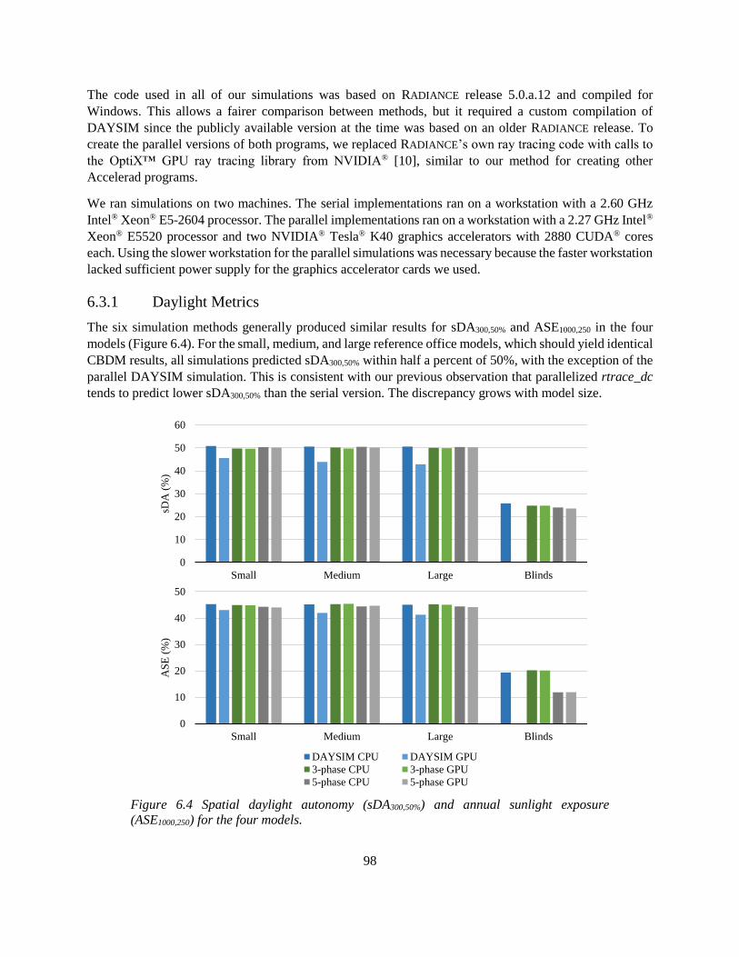
98

The code used in all of our simulations was based on RADIANCE release 5.0.a.12 and compiled for

Windows. This allows a fairer comparison between methods, but it required a custom compilation of

DAYSIM since the publicly available version at the time was based on an older RADIANCE release. To

create the parallel versions of both programs, we replaced RADIANCE’s own ray tracing code with calls to

the OptiX™ GPU ray tracing library from NVIDIA® [10], similar to our method for creating other

Accelerad programs.

We ran simulations on two machines. The serial implementations ran on a workstation with a 2.60 GHz

Intel® Xeon® E5-2604 processor. The parallel implementations ran on a workstation with a 2.27 GHz Intel®

Xeon® E5520 processor and two NVIDIA® Tesla® K40 graphics accelerators with 2880 CUDA® cores

each. Using the slower workstation for the parallel simulations was necessary because the faster workstation

lacked sufficient power supply for the graphics accelerator cards we used.

6.3.1 Daylight Metrics

The six simulation methods generally produced similar results for sDA300,50% and ASE1000,250 in the four

models (Figure 6.4). For the small, medium, and large reference office models, which should yield identical

CBDM results, all simulations predicted sDA300,50% within half a percent of 50%, with the exception of the

parallel DAYSIM simulation. This is consistent with our previous observation that parallelized rtrace_dc

tends to predict lower sDA300,50% than the serial version. The discrepancy grows with model size.

Figure 6.4 Spatial daylight autonomy (sDA300,50%) and annual sunlight exposure

(ASE1000,250) for the four models.

0

10

20

30

40

50

60

Small Medium Large Blinds

sDA

(%

)

0

10

20

30

40

50


AS

E (

%)

DAYSIM CPU DAYSIM GPU

3-phase CPU 3-phase GPU

5-phase CPU 5-phase GPU

99

For the model with blinds, slightly more variation existed between the simulation results. Serial DAYSIM

predicted an sDA300,50% of 26%, while the three- and five-phase methods predicted 24% and 25%

respectively. These discrepancies are well within our error tolerance. However, the parallel DAYSIM

implementation gave poor results. While the simulation did predict some light entering the room, the fixed

size irradiance cache did not register enough diffuse light entering the space to meet the 300-lux threshold

at any sensor.

We saw similar results for ASE1000,250. The parallel DAYSIM results again diverged from the other

simulation methods, which predicted an ASE1000,250 of 45% for the unshaded models. A significant

discrepancy arose between the five-phase method and the other simulation methods for the model with

blinds. The serial DAYSIM simulation and both three-phase method simulations yielded similar ASE1000,250

predictions around 20%, while the five-phase method gave a lower prediction of 12%. The lower value

occurred because the five-phase method’s direct sun-only term did not account for interreflection within

the blinds and was therefore much smaller than the subtracted direct-only component that incorporated the

blinds’ BSDF.

Figure 6.5 shows example results from each of the six simulations. The illuminance snapshots show lighting

conditions under a single sky condition. The relatively small number of sun positions considered by

DAYSIM results in several shadows cast by the window. The three-phase method did not produce well-

defined shadows and instead gave the pattern of light entering through the window a smudged appearance.

The five-phase method considers a large number of sun positions, so it was able to produce a single, hard-

edged shadow. The parallel three- and five-phase simulations produced lower maximum brightness values

than their respective serial versions, but as the maximum values were significantly higher than 1000 lux,

these differences were not apparent in either sDA300,50% or ASE1000,250 results.

6.3.2 Speedup

We ran each simulation in serial on the Intel® Xeon® E5-2604 workstation and in parallel on one and two

Tesla® K40 accelerators. Our concern here lies with the time taken to run rtrace_dc or rcontrib in each

case. Although the matrix algebra performed by ds_illum and dctimestep also added to the total simulation

time, its contribution was relatively minor and in any case was unchanged by parallelizing the ray-tracing

portion of the simulation. For each simulation type, we report the mean runtime from eight simulations.

Table 6.2 breaks down the time taken to compute each matrix in each test, and Figure 6.6 illustrates times

for the small and large models.

In all cases, the three-phase method offered a speed advantage over DAYSIM, whether in parallel or not.

This may come as a surprise given the higher-accuracy parameters recommended for the three-phase

method and may indicate that Russian roulette offers more efficiency than irradiance caching in calculating

diffuse lighting.

Calculation times for the daylight matrices D and Dd show little variance. All of the models we tested had

identical views to the sky from each window, so calculation times did not vary with model size. The GPU

calculation times can be reduced for these matrices by storing the contribution coefficients with single

precision instead of double precision. The calculation was also faster using a single GPU rather than both

together. These facts indicate that loading programs and copying memory to and from the GPUs took up

more time than the calculations themselves. Indeed, calculation of Dd was fast enough on the CPU that

parallelism had no benefit at all.

100

Calculation times for the view matrices V and Vd and the direct sun matrix Cds did benefit from parallelism.

This was particularly true for V, which involved a large number of ray bounces, and Cds, which cast a large

DAYSIM 3-phase 5-phase

CPU GPU CPU GPU CPU GPU

Ref

eren

ce o

ffic

e

Illu

min

an

ce s

nap

sho

t

Da

ylig

ht

au

ton

om

y

Ref

eren

ce o

ffic

e w

ith

bli

nd

s

Illu

min

an

ce s

nap

sho

t

Da

ylig

ht

au

ton

om

y

0 20,000 lux

Figure 6.5 Simulation results of the reference office without and with blinds. Illuminance

snapshots show lighting conditions at 2pm on January 1st. Daylight autonomy images

show regions that achieve 300 lux for at least 50% of occupied hours in white.

101

number of shadow rays because of the number of sun positions. For the smaller models, calculations ran

faster on a single GPU than when using both. The smaller models had only 1425 and 2850 sensors, not

enough to justify the use of a second GPU. (Each GPU had 2880 cores, though we cannot assume a one-to-

one assignment of sensor to core by the graphics driver.) In contrast, the large model had enough sensors

that splitting work between GPUs did result in faster simulations.

Calculation times for the transmission matrix T benefit from parallelism, but only for complex fenestration

systems. In the model with blinds, the BSDF calculation ran twenty-six times faster on a single GPU and

thirty-one times faster on both GPUs. In the models without shading devices, there was no advantage to

Table 6.2 Matrix calculation times by rtrace_dc and rcontrib in minutes.

Model Processor DAYSIM 3-/5-phase 5-phase

Ddir Ddif D T V Dd Vd Cds

Small

CPU 39.2 22.9 1.6 0.1 10.3 0.0 2.1 600.3

1x GPU 8.8 3.9 0.2 0.1 2.3 0.1 0.5 21.1

2x GPU 5.6 2.8 0.7 0.2 3.3 0.6 0.7 45.2

Medium

CPU 78.0 45.5 1.6 0.1 20.9 0.0 4.1 1219.7

1x GPU 12.0 6.3 0.2 0.1 6.2 0.1 1.2 85.6

2x GPU 7.8 4.2 0.7 0.2 6.2 0.6 1.3 73.2

Large

CPU 331.5 177.8 1.7 0.1 111.2 0.0 22.6 6031.0

1x GPU 142.4 117.0 0.2 0.1 32.5 0.2 5.8 374.9

2x GPU 84.6 68.2 0.7 0.2 21.3 0.6 4.4 323.9

Blinds

CPU 96.1 42.9 1.6 21.8 10.1 0.0 2.1 623.5

1x GPU 9.1 4.1 0.2 0.8 2.3 0.1 0.5 21.6

2x GPU 5.8 2.9 0.7 0.7 3.2 0.6 0.7 47.8

Figure 6.6 Cumulative matrix calculation times by rtrace_dc and rcontrib for the small

model (left) and large model (right).

0

10

20

30

40

50

60

Tim

e (m

inu

tes)


614.3

0

100

200

300

400

500

Tim

e (m

inu

tes)


6166.7

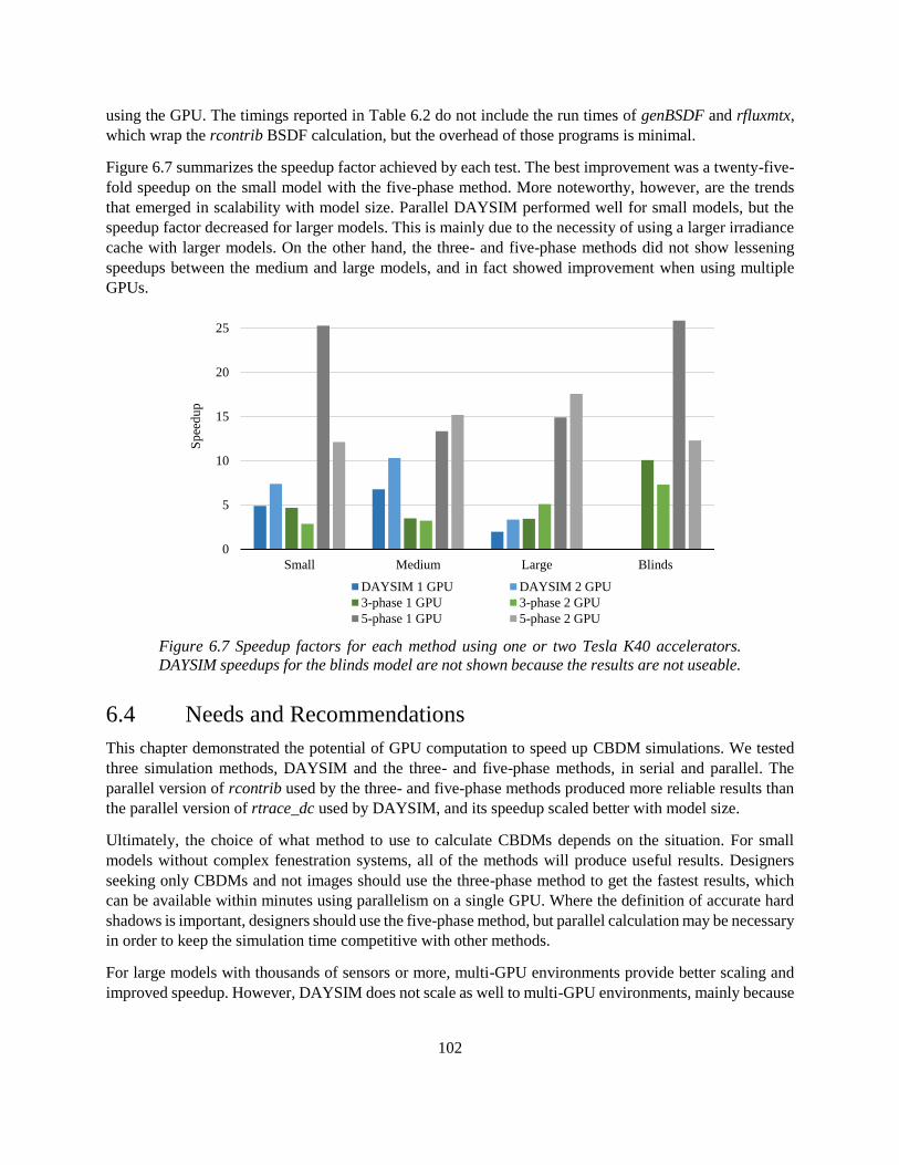
102

using the GPU. The timings reported in Table 6.2 do not include the run times of genBSDF and rfluxmtx,

which wrap the rcontrib BSDF calculation, but the overhead of those programs is minimal.

Figure 6.7 summarizes the speedup factor achieved by each test. The best improvement was a twenty-five-

fold speedup on the small model with the five-phase method. More noteworthy, however, are the trends

that emerged in scalability with model size. Parallel DAYSIM performed well for small models, but the

speedup factor decreased for larger models. This is mainly due to the necessity of using a larger irradiance

cache with larger models. On the other hand, the three- and five-phase methods did not show lessening

speedups between the medium and large models, and in fact showed improvement when using multiple

GPUs.

Figure 6.7 Speedup factors for each method using one or two Tesla K40 accelerators.

DAYSIM speedups for the blinds model are not shown because the results are not useable.

6.4 Needs and Recommendations

This chapter demonstrated the potential of GPU computation to speed up CBDM simulations. We tested

three simulation methods, DAYSIM and the three- and five-phase methods, in serial and parallel. The

parallel version of rcontrib used by the three- and five-phase methods produced more reliable results than

the parallel version of rtrace_dc used by DAYSIM, and its speedup scaled better with model size.

Ultimately, the choice of what method to use to calculate CBDMs depends on the situation. For small

models without complex fenestration systems, all of the methods will produce useful results. Designers

seeking only CBDMs and not images should use the three-phase method to get the fastest results, which

can be available within minutes using parallelism on a single GPU. Where the definition of accurate hard

shadows is important, designers should use the five-phase method, but parallel calculation may be necessary

in order to keep the simulation time competitive with other methods.

For large models with thousands of sensors or more, multi-GPU environments provide better scaling and

improved speedup. However, DAYSIM does not scale as well to multi-GPU environments, mainly because

0

5

10

15

20

25


Sp

eed

up

DAYSIM 1 GPU DAYSIM 2 GPU

3-phase 1 GPU 3-phase 2 GPU

5-phase 1 GPU 5-phase 2 GPU

103

of its reliance on irradiance caching. Similarly, DAYSIM is not a reliable platform for analysing complex

fenestration systems, especially in parallel. Designers should therefore use the GPU-based three- and five-

phase methods when working with large models.

This study also reveals some shortcomings of simulation models and currently available hardware. There

are a number of factors that must be considered to improve speeds in future work:

Models need more potential for parallelism. Image generation assigns one primary ray to each pixel,

such that a 512 × 512 image has 262,144 primary rays that may be traced in parallel. Irradiance sensor

simulation assigns only one primary ray to each sensor, however, resulting in many fewer rays that

could be traced in parallel. With only 1425 primary rays, we do not even take advantage of all the cores

available on our GPUs. In the future, we expect designers to simulate larger models, which will

naturally result in an increased potential for parallelism.

Faster memory access and more efficient daylight coefficient storage are needed. CBDM calculation

adds to Accelerad the need to store a large amount of frequently accessed data in the GPU’s global

memory. The memory requirement grows with the number of sensor points and, in the case of

rtrace_dc, with the size of the irradiance cache as well. At the same time, daylight coefficient and

contribution coefficient arrays are often sparse, and static allocation of daylight coefficient arrays

necessarily leaves space for more bounces than are likely to be calculated. Condensing memory

requirements and accelerating memory access will result in faster simulations.

Graphics accelerator capabilities must increase. As shown in Figure 6.7, increasing the number of cores

on a GPU is significantly more effective at improving performance than increasing the number of

GPUs. Daylight coefficient calculation is well positioned to take advantage of the current trend toward

increased core counts [41].

Many of these factors will also help to improve the accuracy of daylight coefficient calculation on the GPU.

However, even in its current state, the error in daylight autonomy and annual sun exposure calculations is

small and clearly acceptable for early design stages.

105

7 Real-Time Glare Analysis

In this chapter, we replace the ray-tracing algorithm normally used by RADIANCE and Accelerad with

progressive path tracing. The chapter presents the results of two studies. The first study, Real-time visual

comfort feedback for architectural design, was published in 2016 [20]. It describes an Accelerad version of

rvu, a graphic interface for generating RADIANCE images, which can display live-updating predictions of

daylight glare probability, task luminance, and contrast alongside a progressively rendered image of the

scene. Users may decide when to accept the progressively refining values and move on with the design

process. In most cases, sufficiently accurate results are available within seconds, after rendering only a few

frames.

The second study, Effects of real-time simulation feedback on design for visual comfort, is currently under

preparation. It describes a study in which forty human subjects with backgrounds in building design and

technology carried out two shading design exercises to balance glare reduction and annual daylight

availability in two open office arrangements using two simulation tools with differing system response

times. Subjects with access to real-time simulation feedback tested more design options, reported higher

confidence in design quality and increased satisfaction with the design task, and produced better-performing

final designs regarding daylight autonomy and daylight glare probability.

7.1 Progressive Path Tracing

In our previous studies, Accelerad has allowed hours-long RADIANCE simulations to run in minutes, but it

has not achieved real-time speeds. In an effort to improve rendering quality and speed, the computer

graphics community has produced many alternative methods for computing global illumination. One

alternative is path tracing, which traces only a single ray from each intersection but does so iteratively in

order to build up a complete sampling of the scene [161]. Path tracing and many of its extensions offer the

benefit that intermediate results may be displayed before the rendering is finished. When a render displays

intermediate results of a path tracing simulation as they become available, this is termed progressive path

tracing.

We modified the RADIANCE source code to perform progressive path tracing on the GPU with the OptiX™

ray-tracing engine [10]. By default, RADIANCE allows the user to specify the number of ambient divisions

for diffuse sampling. In our implementation, the number of ambient divisions is held at one, and instead of

achieving better accuracy through sampling density, we achieve it using multiple rendering passes. The

first pass (frame zero) traces only direct and specular paths. Subsequent passes calculate the diffuse

component at low accuracy. The results are aggregated and progressively refined for each pixel as follows:

𝐿𝑝,𝑛′ = 𝐿𝑝,0 +

1

𝑛∑𝐿𝑝,𝑖

𝑛

𝑖=1

(7.1)

where Lp,i is the luminance returned by the ith ray through pixel p, and L’p,n is the luminance of that pixel

after n frames. The ray intersection routines, though carried out on the GPU, remain identical to those in

RADIANCE, so the results after aggregating a large number of frames are also expected to be identical to

RADIANCE.

106

Figure 7.1 The prototype’s user interface presents live views of the rendering in progress

and predicted visual comfort values.

Post-processing and calculation of metrics is split between the GPU and CPU. Pixel-level calculations

including luminance calculation occur in parallel on the GPU, while the summations required to calculate

the visual comfort metrics occur on the CPU. Tone-mapping for scene visualization also occurs on the

GPU, and while the high-dynamic range (HDR) pixel values are stored on the GPU and may be saved to a

RADIANCE HDR file upon request, only the tone-mapped image is returned to the CPU for display at every

frame.

The graphic user interface for an early prototype is modified from the rvu program included with RADIANCE

(Figure 7.1). The user may choose between photorealistic tone mapping and false color visualization using

the same options that are available in Thomas Bleicher’s wxfalsecolor program. We recommend the use of

false color because the HDR extents of many daylit scenes exceed the viewable range on most monitors.

Our prototype can calculate several image-based metrics, including vertical eye illuminance (Ev), daylight

glare probability (DGP), task area luminance (TAL), and contrast ratio (CRv or CRd). In its current

implementation, the interface allows a single task area and pair of contrast regions to be monitored by the

TAL and CRv metrics. However, nothing prevents further development from allowing an unlimited number

of regions within the image to be monitored simultaneously. A separate window displays a frame-by-frame

history of visual comfort metric values.

7.2 Prototype Tests

We tested our prototype in ten scenes. The scenes were modeled in either Rhinoceros or SketchUp; the

Rhinoceros models were exported to RADIANCE format using DIVA-for-Rhino [155], and the SketchUp

models were exported using Thomas Bleicher’s su2rad. Our prototype makes all RADIANCE projections

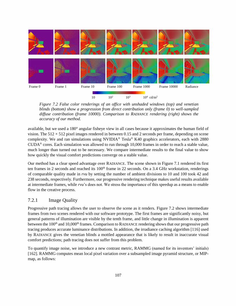
107

available, but we used a 180° angular fisheye view in all cases because it approximates the human field of

vision. The 512 × 512 pixel images rendered in between 0.15 and 2 seconds per frame, depending on scene

complexity. We and ran simulations using NVIDIA® Tesla® K40 graphics accelerators, each with 2880

CUDA® cores. Each simulation was allowed to run through 10,000 frames in order to reach a stable value,

much longer than turned out to be necessary. We compare intermediate results to the final value to show

how quickly the visual comfort predictions converge on a stable value.

Our method has a clear speed advantage over RADIANCE. The scene shown in Figure 7.1 rendered its first

ten frames in 2 seconds and reached its 100th frame in 22 seconds. On a 3.4 GHz workstation, renderings

of comparable quality made in rvu by setting the number of ambient divisions to 10 and 100 took 42 and

238 seconds, respectively. Furthermore, our progressive rendering technique makes useful results available

at intermediate frames, while rvu’s does not. We stress the importance of this speedup as a means to enable

flow in the creative process.

7.2.1 Image Quality

Progressive path tracing allows the user to observe the scene as it renders. Figure 7.2 shows intermediate

frames from two scenes rendered with our software prototype. The first frames are significantly noisy, but

general patterns of illumination are visible by the tenth frame, and little change in illumination is apparent

between the 100th and 10,000th frames. Comparison to RADIANCE rendering shows that our progressive path

tracing produces accurate luminance distributions. In addition, the irradiance caching algorithm [116] used

by RADIANCE gives the venetian blinds a mottled appearance that is likely to result in inaccurate visual

comfort predictions; path tracing does not suffer from this problem.

To quantify image noise, we introduce a new contrast metric, RAMMG (named for its inventors’ initials)

[162]. RAMMG computes mean local pixel variation over a subsampled image pyramid structure, or MIP-

map, as follows:

Frame 0 Frame 1 Frame 10 Frame 100 Frame 1000 Frame 10000 Radiance

10 102 103 104 cd/m2

Figure 7.2 False color renderings of an office with unshaded windows (top) and venetian

blinds (bottom) show a progression from direct contribution only (frame 0) to well-sampled

diffuse contribution (frame 10000). Comparison to RADIANCE rendering (right) shows the

accuracy of our method.

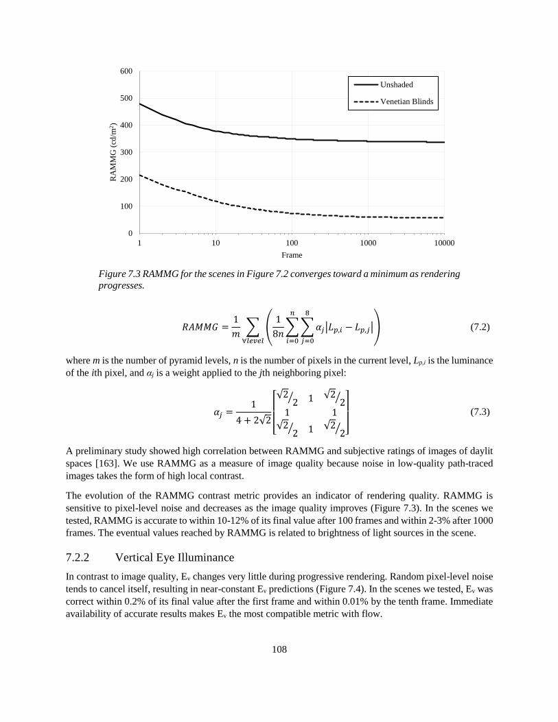
108

Figure 7.3 RAMMG for the scenes in Figure 7.2 converges toward a minimum as rendering

progresses.

𝑅𝐴𝑀𝑀𝐺 =1

𝑚∑ (

1

8𝑛∑∑𝛼𝑗|𝐿𝑝,𝑖 − 𝐿𝑝,𝑗|

8

𝑗=0

𝑛

𝑖=0

)

∀𝑙𝑒𝑣𝑒𝑙

(7.2)

where m is the number of pyramid levels, n is the number of pixels in the current level, Lp,i is the luminance

of the ith pixel, and αj is a weight applied to the jth neighboring pixel:

𝛼𝑗 =1

4 + 2√2[ √2

2⁄ 1 √2

2⁄

1 1

√22

⁄ 1 √22

⁄ ]

(7.3)

A preliminary study showed high correlation between RAMMG and subjective ratings of images of daylit

spaces [163]. We use RAMMG as a measure of image quality because noise in low-quality path-traced

images takes the form of high local contrast.

The evolution of the RAMMG contrast metric provides an indicator of rendering quality. RAMMG is

sensitive to pixel-level noise and decreases as the image quality improves (Figure 7.3). In the scenes we

tested, RAMMG is accurate to within 10-12% of its final value after 100 frames and within 2-3% after 1000

frames. The eventual values reached by RAMMG is related to brightness of light sources in the scene.

7.2.2 Vertical Eye Illuminance

In contrast to image quality, Ev changes very little during progressive rendering. Random pixel-level noise

tends to cancel itself, resulting in near-constant Ev predictions (Figure 7.4). In the scenes we tested, Ev was

correct within 0.2% of its final value after the first frame and within 0.01% by the tenth frame. Immediate

availability of accurate results makes Ev the most compatible metric with flow.

0

100

200

300

400

500

600

1 10 100 1000 10000

RA

MM

G (

cd/m

2)

Frame

Unshaded

Venetian Blinds

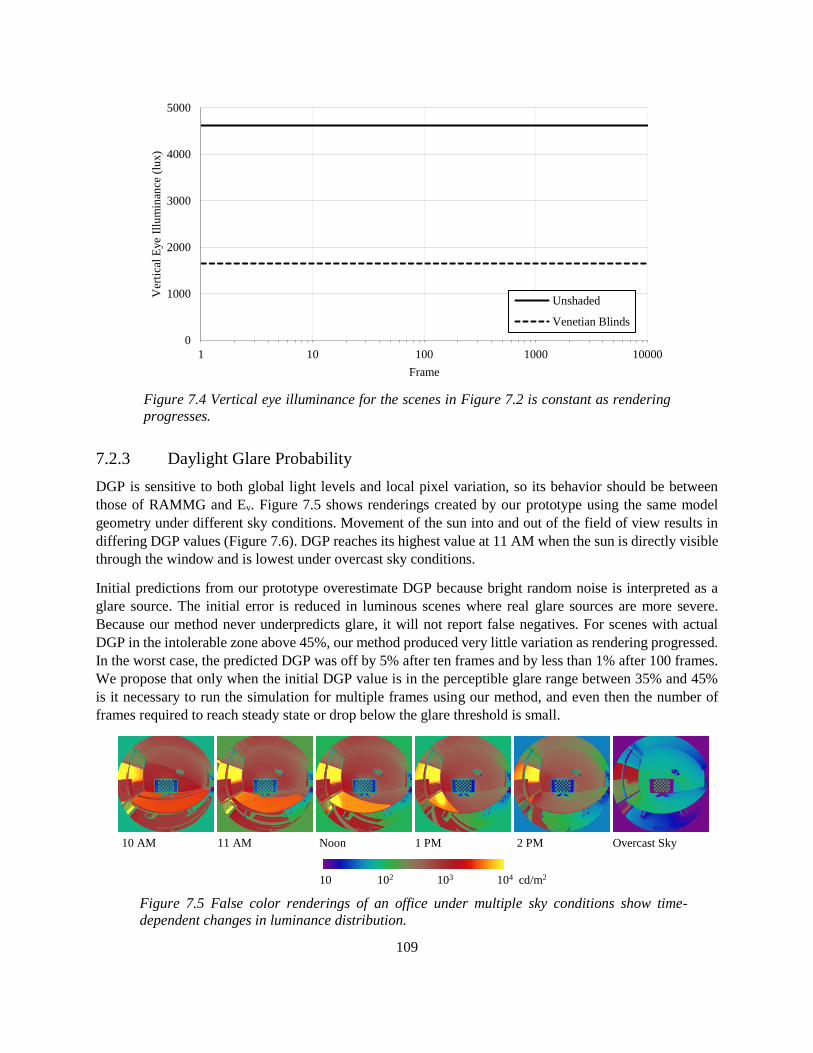
109

Figure 7.4 Vertical eye illuminance for the scenes in Figure 7.2 is constant as rendering

progresses.

7.2.3 Daylight Glare Probability

DGP is sensitive to both global light levels and local pixel variation, so its behavior should be between

those of RAMMG and Ev. Figure 7.5 shows renderings created by our prototype using the same model

geometry under different sky conditions. Movement of the sun into and out of the field of view results in

differing DGP values (Figure 7.6). DGP reaches its highest value at 11 AM when the sun is directly visible

through the window and is lowest under overcast sky conditions.

Initial predictions from our prototype overestimate DGP because bright random noise is interpreted as a

glare source. The initial error is reduced in luminous scenes where real glare sources are more severe.

Because our method never underpredicts glare, it will not report false negatives. For scenes with actual

DGP in the intolerable zone above 45%, our method produced very little variation as rendering progressed.

In the worst case, the predicted DGP was off by 5% after ten frames and by less than 1% after 100 frames.

We propose that only when the initial DGP value is in the perceptible glare range between 35% and 45%

is it necessary to run the simulation for multiple frames using our method, and even then the number of

frames required to reach steady state or drop below the glare threshold is small.

0

1000

2000

3000

4000

5000

1 10 100 1000 10000

Ver

tica

l E

ye

Illu

min

ance

(lu

x)

Frame

Unshaded

Venetian Blinds

10 AM 11 AM Noon 1 PM 2 PM Overcast Sky

10 102 103 104 cd/m2

Figure 7.5 False color renderings of an office under multiple sky conditions show time-

dependent changes in luminance distribution.

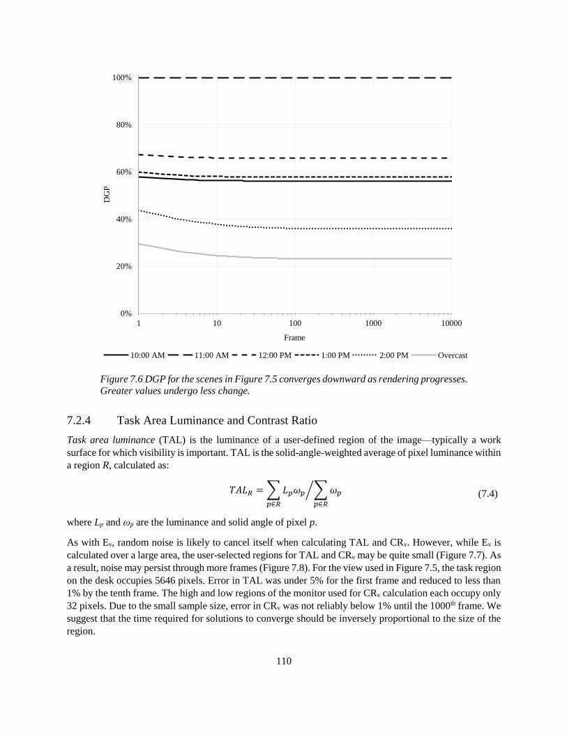
110

Figure 7.6 DGP for the scenes in Figure 7.5 converges downward as rendering progresses.

Greater values undergo less change.

7.2.4 Task Area Luminance and Contrast Ratio

Task area luminance (TAL) is the luminance of a user-defined region of the image—typically a work

surface for which visibility is important. TAL is the solid-angle-weighted average of pixel luminance within

a region R, calculated as:

𝑇𝐴𝐿𝑅 = ∑ 𝐿𝑝𝜔𝑝

𝑝∈𝑅

∑ 𝜔𝑝

𝑝∈𝑅

⁄ (7.4)

where Lp and ωp are the luminance and solid angle of pixel p.

As with Ev, random noise is likely to cancel itself when calculating TAL and CRv. However, while Ev is

calculated over a large area, the user-selected regions for TAL and CRv may be quite small (Figure 7.7). As

a result, noise may persist through more frames (Figure 7.8). For the view used in Figure 7.5, the task region

on the desk occupies 5646 pixels. Error in TAL was under 5% for the first frame and reduced to less than

1% by the tenth frame. The high and low regions of the monitor used for CRv calculation each occupy only

32 pixels. Due to the small sample size, error in CRv was not reliably below 1% until the 1000th frame. We

suggest that the time required for solutions to converge should be inversely proportional to the size of the

region.

0%

20%

40%

60%

80%

100%

1 10 100 1000 10000

DG

P

Frame

10:00 AM 11:00 AM 12:00 PM 1:00 PM 2:00 PM Overcast

111

Figure 7.7 The user-specified regions for calculating TAL and CR are small relative to the

entire rendering.

Figure 7.8 TAL (above) and CRv (below) for the scenes in Figure 7.5 show varying random

noise depending on the number of pixels in the region.

CR Low Region

CR High Region

TAL Region

Ev Region

0

500

1000

1500

2000

2500

3000

3500

4000

4500

5000

1 10 100 1000 10000

TA

L (

cd/m

2)

0

0.1

0.2

0.3

1 10 100 1000 10000

Co

ntr

ast

Rat

io

Frame

10:00 AM 11:00 AM 12:00 PM 1:00 PM 2:00 PM Overcast

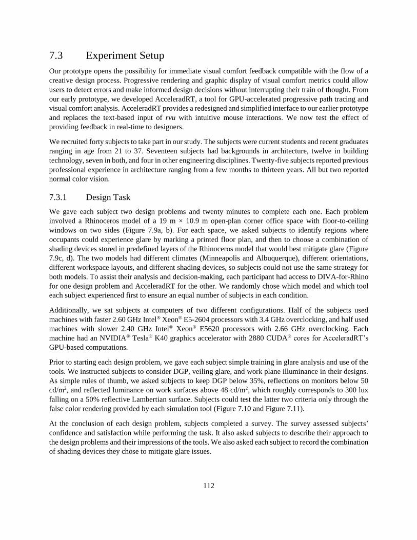
112

7.3 Experiment Setup

Our prototype opens the possibility for immediate visual comfort feedback compatible with the flow of a

creative design process. Progressive rendering and graphic display of visual comfort metrics could allow

users to detect errors and make informed design decisions without interrupting their train of thought. From

our early prototype, we developed AcceleradRT, a tool for GPU-accelerated progressive path tracing and

visual comfort analysis. AcceleradRT provides a redesigned and simplified interface to our earlier prototype

and replaces the text-based input of rvu with intuitive mouse interactions. We now test the effect of

providing feedback in real-time to designers.

We recruited forty subjects to take part in our study. The subjects were current students and recent graduates

ranging in age from 21 to 37. Seventeen subjects had backgrounds in architecture, twelve in building

technology, seven in both, and four in other engineering disciplines. Twenty-five subjects reported previous

professional experience in architecture ranging from a few months to thirteen years. All but two reported

normal color vision.

7.3.1 Design Task

We gave each subject two design problems and twenty minutes to complete each one. Each problem

involved a Rhinoceros model of a 19 m × 10.9 m open-plan corner office space with floor-to-ceiling

windows on two sides (Figure 7.9a, b). For each space, we asked subjects to identify regions where

occupants could experience glare by marking a printed floor plan, and then to choose a combination of

shading devices stored in predefined layers of the Rhinoceros model that would best mitigate glare (Figure

7.9c, d). The two models had different climates (Minneapolis and Albuquerque), different orientations,

different workspace layouts, and different shading devices, so subjects could not use the same strategy for

both models. To assist their analysis and decision-making, each participant had access to DIVA-for-Rhino

for one design problem and AcceleradRT for the other. We randomly chose which model and which tool

each subject experienced first to ensure an equal number of subjects in each condition.

Additionally, we sat subjects at computers of two different configurations. Half of the subjects used

machines with faster 2.60 GHz Intel® Xeon® E5-2604 processors with 3.4 GHz overclocking, and half used

machines with slower 2.40 GHz Intel® Xeon® E5620 processors with 2.66 GHz overclocking. Each

machine had an NVIDIA® Tesla® K40 graphics accelerator with 2880 CUDA® cores for AcceleradRT’s

GPU-based computations.

Prior to starting each design problem, we gave each subject simple training in glare analysis and use of the

tools. We instructed subjects to consider DGP, veiling glare, and work plane illuminance in their designs.

As simple rules of thumb, we asked subjects to keep DGP below 35%, reflections on monitors below 50

cd/m2, and reflected luminance on work surfaces above 48 cd/m2, which roughly corresponds to 300 lux

falling on a 50% reflective Lambertian surface. Subjects could test the latter two criteria only through the

false color rendering provided by each simulation tool (Figure 7.10 and Figure 7.11).

At the conclusion of each design problem, subjects completed a survey. The survey assessed subjects’

confidence and satisfaction while performing the task. It also asked subjects to describe their approach to

the design problems and their impressions of the tools. We also asked each subject to record the combination

of shading devices they chose to mitigate glare issues.

113

Minneapolis Albuquerque

a b

No Shading Overhang No Shading Additional Mullions

Spandrel Vertical Fins Spandrels Light Shelf

Horizontal Louvers Diagonal Louvers Vertical Fins Inverted Louvers

c d

Figure 7.9 Floor plans of the two models used for the (a) Minneapolis and (b) Albuquerque

climates and (c and d) the shading device options for each.

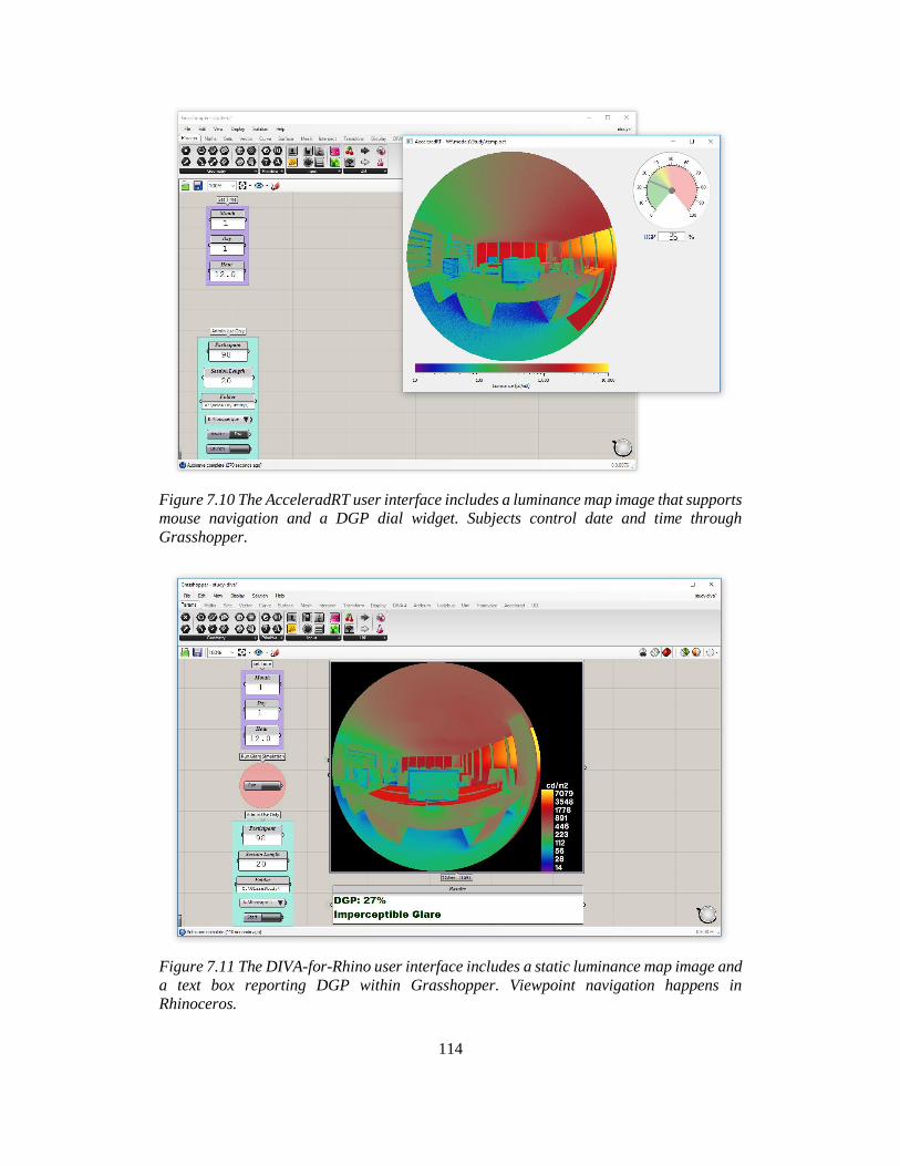
114

Figure 7.10 The AcceleradRT user interface includes a luminance map image that supports

mouse navigation and a DGP dial widget. Subjects control date and time through

Grasshopper.

Figure 7.11 The DIVA-for-Rhino user interface includes a static luminance map image and

a text box reporting DGP within Grasshopper. Viewpoint navigation happens in

Rhinoceros.

115

7.3.2 Tool Design

We created a customized workflow for each tool that gave subjects access to four input parameters: layer

state, date and time, view, and simulation initiation. Subjects added or removed shading devices from the

Rhinoceros model using the layer panel within the main Rhinoceros window (Figure 7.12). We provided

month, date, and hour controls within a Grasshopper visual programming interface for both tools. For

DIVA-for-Rhino, we provided an object in the Rhinoceros model to serve as an avatar to choose position

and viewing direction. Subjects could move and rotate the avatar using Rhinoceros’ gumball navigation

(shown in Figure 7.12). We chose this method because preliminary trials showed that subjects had difficulty

placing the virtual camera if they could not see its location. Because AcceleradRT features an animated

progressive rendering rather than a static image, users can navigate the scene with mouse gestures over the

image. We used Grasshopper to place an avatar in the Rhinoceros viewport to show the current view, but

subjects controlled the position and view direction through AcceleradRT rather than Rhinoceros. In both

instances, the avatars held the viewpoint at 1.3 m above the floor, corresponding to a typical seated eye

level. Finally, we provided a Grasshopper button to start the simulation process in DIVA-for-Rhino. After

setting the desired layer state, time, and view, subjects could click the button to initiate a simulation using

DIVA-for-Rhino’s lowest quality setting. AcceleradRT performs simulations continuously, so its interface

offered no equivalent feature.

Figure 7.12 The Rhinoceros interface used with both tools includes the layer controls

(right) and avatar, shown here with the gumball navigation control used in DIVA-for-

Rhino.

The output from both tools is primarily graphical. We set up both tools to display the avatar’s current view

in 180° equiangular fisheye projection using a logarithmic false color scale from 10 – 10,000 cd/m2. This

display allowed subjects to estimate the brightness of spots such as monitors and work surfaces in the

116

model. In DIVA-for-Rhino, we displayed the DGP value in a prominent text box. AcceleradRT displays

DGP using a dial widget with green and red coloring to represent acceptable and unacceptable values,

respectively (shown in Figure 7.10).

We used a custom Grasshopper component to log each subject’s layer state, time, view and simulation

interactions for both tools. A timestamp associated with each interaction allowed us to record the length of

time a subject spent in each combination of layer state, time, and view, and for DIVA-for-Rhino the elapsed

time during simulation runs.

7.4 User Study Results

Forty subjects collectively give us 800 minutes of recorded user interaction for each tool. We analyze this

data in three ways. First, we examine the user behaviors, processes, and strategies that subjects employed

to see how they differed depending on the tool used. Second, we examine the proposed designs from each

subject to see if the choice of tool affected design performance. Finally, we examine the subjects’ survey

responses to see if subjects developed preferences for the tools.

7.4.1 User Behaviors and Design Strategies

Given the lack of best-practice information on how to design for occupant-centric visual comfort, subjects’

behaviors varied widely. Their self-reported design processes show several different approaches. Some

chose to consider only a few key times, particularly with low sun angles on solstices, while other scanned

many more times. Some concentrated on finding critical views, while others explored the space more fully.

Some subjects showed concern for whether certain parts of the space were likely to be occupied and

concentrated on views that faced computer screens in the models. Some were systematic in trying all

shading devices early on, while others waited to gain a more complete understanding of the initial

conditions first, and with each tool, 10% ran out of time before trying any shading devices.

We are interested in the amount of information that subjects accumulated while making their design

decisions, and therefore we want to know how many views, times, and layers states subjects explored (Table

7.1). However, setting the desired configuration of view, time, or layer state might involve multiple

interactions to set the month, date, hour, x- and y-positions, view rotation angle, or visibility states of

multiple layers. Rather than counting the total number of interactions, we count only those that preceded

sufficiently long pauses to indicate that the subject might have thought about the result. However, the time

this takes may vary depending on context [24]. Using DIVA-for-Rhino, simulations took on average 20

seconds using the faster computers and 29 seconds using the slower computers, so we can assume that a

series of interactions within a shorter timeframe form a unit task such as setting up a time and viewpoint

for the next simulation. Using AcceleradRT, where preliminary results are available in real time, subjects

might reject an idea after rendering only a few frames if the results did not look promising. Each frame

takes approximately 200 ms to render, so a series of interactions over a period of several seconds might

represent individual cognitive operations as the user queries more information about the scene. In two

seconds, AcceleradRT renders about ten frames, by which point global metrics such as DGP tend to stabilize

in the animation. We choose two seconds as the minimum duration below which the subjects were unlikely

to gain information about a design.

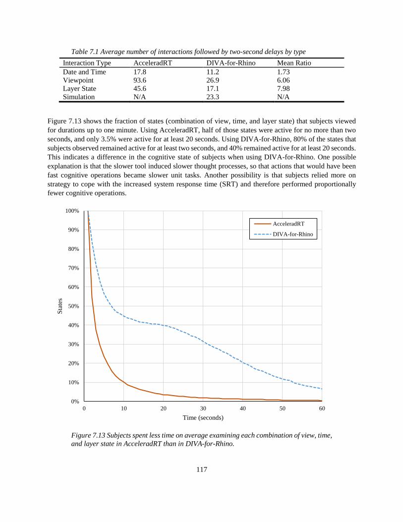
117

Table 7.1 Average number of interactions followed by two-second delays by type

Interaction Type AcceleradRT DIVA-for-Rhino Mean Ratio

Date and Time 17.8 11.2 1.73

Viewpoint 93.6 26.9 6.06

Layer State 45.6 17.1 7.98

Simulation N/A 23.3 N/A

Figure 7.13 shows the fraction of states (combination of view, time, and layer state) that subjects viewed

for durations up to one minute. Using AcceleradRT, half of those states were active for no more than two

seconds, and only 3.5% were active for at least 20 seconds. Using DIVA-for-Rhino, 80% of the states that

subjects observed remained active for at least two seconds, and 40% remained active for at least 20 seconds.

This indicates a difference in the cognitive state of subjects when using DIVA-for-Rhino. One possible

explanation is that the slower tool induced slower thought processes, so that actions that would have been

fast cognitive operations became slower unit tasks. Another possibility is that subjects relied more on

strategy to cope with the increased system response time (SRT) and therefore performed proportionally

fewer cognitive operations.

Figure 7.13 Subjects spent less time on average examining each combination of view, time,

and layer state in AcceleradRT than in DIVA-for-Rhino.

0%

10%

20%

30%

40%

50%

60%

70%

80%

90%

100%

0 10 20 30 40 50 60

Sta

tes

Time (seconds)

AcceleradRT

DIVA-for-Rhino

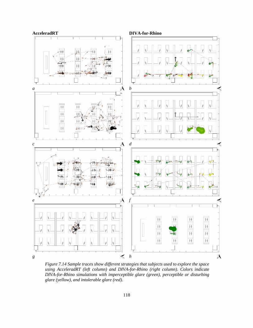
118

AcceleradRT DIVA-for-Rhino

a b

c d

e f

g h

Figure 7.14 Sample traces show different strategies that subjects used to explore the space

using AcceleradRT (left column) and DIVA-for-Rhino (right column). Colors indicate

DIVA-for-Rhino simulations with imperceptible glare (green), perceptible or disturbing

glare (yellow), and intolerable glare (red).

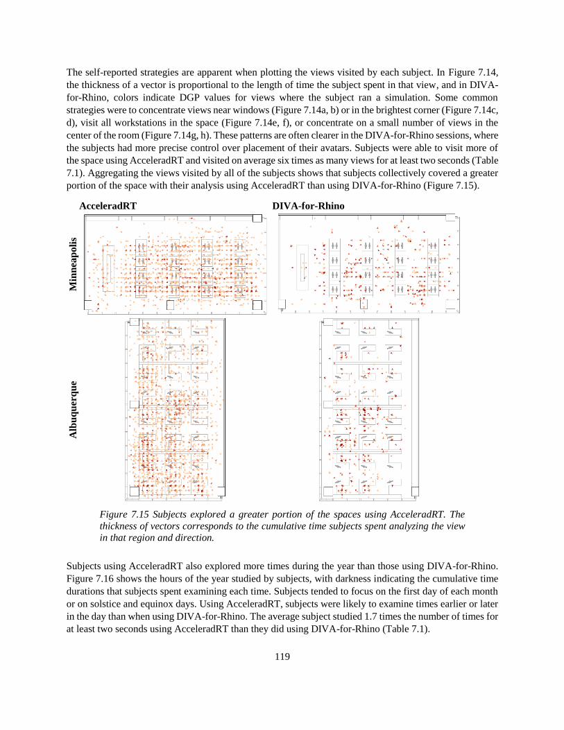
119

The self-reported strategies are apparent when plotting the views visited by each subject. In Figure 7.14,

the thickness of a vector is proportional to the length of time the subject spent in that view, and in DIVA-

for-Rhino, colors indicate DGP values for views where the subject ran a simulation. Some common

strategies were to concentrate views near windows (Figure 7.14a, b) or in the brightest corner (Figure 7.14c,

d), visit all workstations in the space (Figure 7.14e, f), or concentrate on a small number of views in the

center of the room (Figure 7.14g, h). These patterns are often clearer in the DIVA-for-Rhino sessions, where

the subjects had more precise control over placement of their avatars. Subjects were able to visit more of

the space using AcceleradRT and visited on average six times as many views for at least two seconds (Table

7.1). Aggregating the views visited by all of the subjects shows that subjects collectively covered a greater

portion of the space with their analysis using AcceleradRT than using DIVA-for-Rhino (Figure 7.15).


Min

nea

po

lis

Alb

uq

uer

qu

e

Figure 7.15 Subjects explored a greater portion of the spaces using AcceleradRT. The

thickness of vectors corresponds to the cumulative time subjects spent analyzing the view

in that region and direction.

Subjects using AcceleradRT also explored more times during the year than those using DIVA-for-Rhino.

Figure 7.16 shows the hours of the year studied by subjects, with darkness indicating the cumulative time

durations that subjects spent examining each time. Subjects tended to focus on the first day of each month

or on solstice and equinox days. Using AcceleradRT, subjects were likely to examine times earlier or later

in the day than when using DIVA-for-Rhino. The average subject studied 1.7 times the number of times for

at least two seconds using AcceleradRT than they did using DIVA-for-Rhino (Table 7.1).

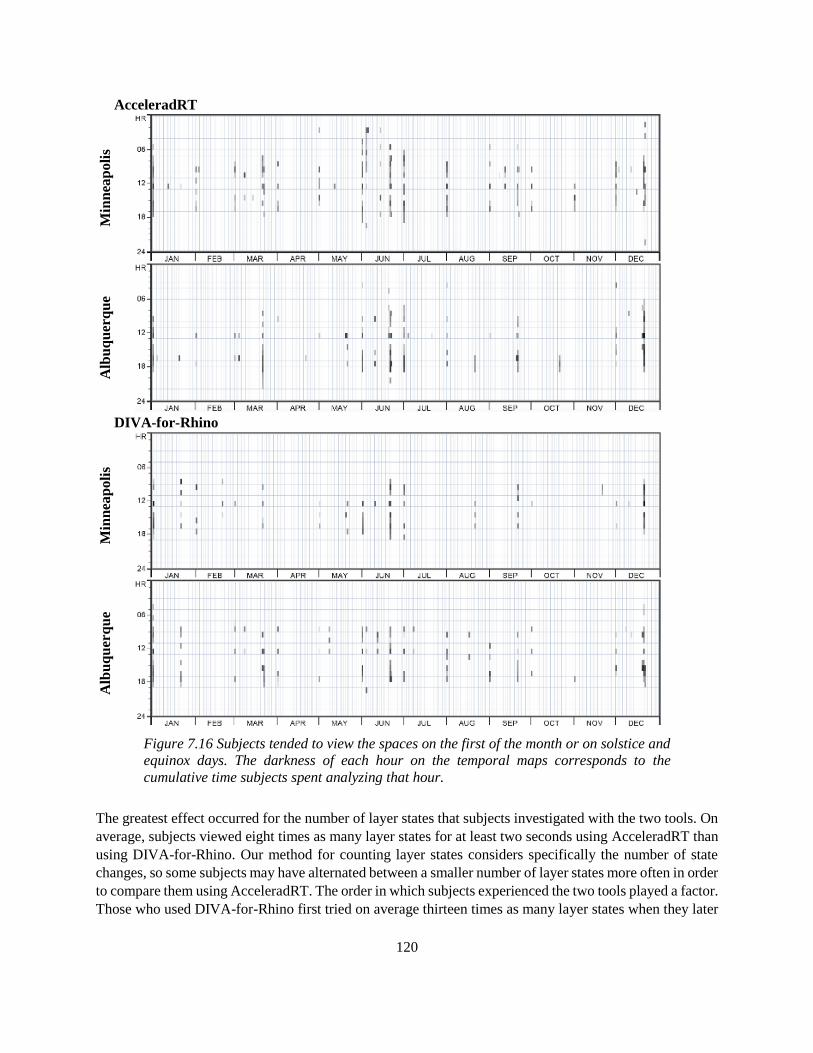
120

AcceleradRT M

inn

eap

oli

s

Alb

uq

uer

qu

e

DIVA-for-Rhino

Min

nea

poli

s

Alb

uq

uer

qu

e

Figure 7.16 Subjects tended to view the spaces on the first of the month or on solstice and

equinox days. The darkness of each hour on the temporal maps corresponds to the

cumulative time subjects spent analyzing that hour.

The greatest effect occurred for the number of layer states that subjects investigated with the two tools. On

average, subjects viewed eight times as many layer states for at least two seconds using AcceleradRT than

using DIVA-for-Rhino. Our method for counting layer states considers specifically the number of state

changes, so some subjects may have alternated between a smaller number of layer states more often in order

to compare them using AcceleradRT. The order in which subjects experienced the two tools played a factor.

Those who used DIVA-for-Rhino first tried on average thirteen times as many layer states when they later

121

used AcceleradRT, while those who used AcceleradRT first tried on average only three times more layer

states than they did later with DIVA-for-Rhino (Table 7.1). We reason that early exposure to the faster tool

conditioned subjects to explore the design space more thoroughly.

A temporal view of user behavior offers another window into the strategies that subject employed. In Figure

7.17, colored dots represent different types of subject interactions. Most subjects alternated between spatial

explorations and changing the layer state, with infrequent changes to the time. This may be because the

time controls required keyboard interaction and therefore seemed to involve more effort from the subjects.

Using DIVA-for-Rhino, most subjects adopted a pattern of changing either view or layer state followed by

running a simulation, and the frequency of interaction stayed relatively constant for each subject. Using

AcceleradRT, subjects displayed a much higher frequency of interaction, with many views and layer states

observed for only a matter of seconds. A quarter of subjects entered a prolonged period of inactivity ranging

from one to five minutes, usually toward the end of the twenty-minute session. This inactivity may indicate

the need for a break, attention turning to the printed floor plans instead of the screen, or early completion

of the task. We did observe periods of inactivity using DIVA-for-Rhino as well, but they are generally

shorter and occur earlier in the sessions. This may indicate hesitance to start the task due to the less intuitive

interface.

With DIVA-for-Rhino only, we can examine the effect of processor speed on user behavior. Subjects using

faster computers examined 50% more view and 30% more layer states, and ran 37% more simulations than

subjects using the slower computers. Subjects using faster computers also spent less time reviewing results

or changing the model between simulations; there was almost no difference in the fraction of time taken up

by simulations between the two groups (45% for subjects with fast computers versus 48% for subjects with

slow computers). This may indicate that subjects who had to wait longer for simulation results became

distracted more often, valued the time in which they could interact with the models more, or were otherwise

less inclined to run simulations.

7.4.2 Design Performance

In order to judge the quality of the designs that subjects proposed, we ran several performance simulations

on each model with each possible combination of shading devices. No widely accepted metric for visual

comfort accounts for both spatial and temporal luminance variation, and we do not aim to promote one

here. We calculated four daylighting performance metrics that relate to visual discomfort: sDA300,50%,

ASE1000,250, fraction of occupied hours of direct visibility of the solar disk, and fraction of occupied hours

in which DGPs exceeded 35% (see Equation (2.6)). For each metric, we divided the space according to a

0.5-m square grid of 819 sensors. We calculated the first two metrics at a work plane elevation of 78 cm,

and the others at a seated head height of 130 cm. For solar disk visibility, we report the mean value across

all 819 sensor. We measured DGPs in eight equally spaced directions at each sensor, and we report the

average across all directions and sensors. All four metrics tend to increase as the unobstructed view to the

sky increases (Figure 7.18). This results in two competing goals, as we prefer to maintain a high sDA300,50%

while reducing the other metrics. We can define high-performing designs as those on the Pareto front that

maximizes sDA300,50% while minimizing the potential for glare as measured by DGPs.

122


Event types: time, view, layer state, simulation

Figure 7.17 Timelines of subject interactions with the simulation tools show greater

interaction with AcceleradRT and more regularly spaced interaction with DIVA-for-

Rhino.

123

Minneapolis Albuquerque

Figure 7.18 Shading designs chosen using AcceleradRT were more likely to lie close to the

Pareto front (high sDA300,50% and low ASE1000,250, solar disk visibility, or DGPs) than those

chosen using DIVA-for-Rhino.

0%

20%

40%

60%

80%

100%

0% 20% 40% 60% 80% 100%

AS

E

sDA

Not ChosenAccel: 1Accel: 2Accel: 3Accel: >3DIVA: 1DIVA: 2DIVA: 3DIVA: >3

0%

20%

40%

60%

80%

100%

0% 20% 40% 60% 80% 100%

AS

E

sDA

0%

2%

4%

6%

8%

10%

12%

14%

16%

0% 20% 40% 60% 80% 100%

So

lar

Dis

k V

isib

ilit

y

sDA

0%

2%

4%

6%

8%

10%

12%

14%

16%

0% 20% 40% 60% 80% 100%

So

lar

Dis

k V

isib

ilit

y

sDA

0%

5%

10%

15%

20%

25%

30%

0% 20% 40% 60% 80% 100%

DG

Ps

sDA

0%

5%

10%

15%

20%

25%

30%

0% 20% 40% 60% 80% 100%

DG

Ps

sDA

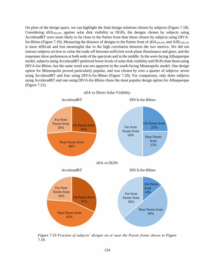
124

On plots of the design space, we can highlight the final design solutions chosen by subjects (Figure 7.18).

Considering sDA300,50% against solar disk visibility or DGPs, the designs chosen by subjects using

AcceleradRT were more likely to lie close to the Pareto front than those chosen by subjects using DIVA-

for-Rhino (Figure 7.19). Measuring the distance of designs to the Pareto front of sDA300,50% and ASE1000,250

is more difficult and less meaningful due to the high correlation between the two metrics. We did not

instruct subjects on how to value the trade-off between sufficient work plane illuminance and glare, and the

responses show preferences at both ends of the spectrum and in the middle. In the west-facing Albuquerque

model, subjects using AcceleradRT preferred lower levels of solar disk visibility and DGPs than those using

DIVA-for-Rhino, but the same trend was not apparent in the south-facing Minneapolis model. One design

option for Minneapolis proved particularly popular, and was chosen by over a quarter of subjects: seven

using AcceleradRT and four using DIVA-for-Rhino (Figure 7.20). For comparison, only three subjects

using AcceleradRT and one using DIVA-for-Rhino chose the most popular design option for Albuquerque

(Figure 7.21).

sDA vs Direct Solar Visibility

sDA vs DGPs

Figure 7.19 Fraction of subjects’ designs on or near the Pareto fronts shown in Figure

7.18.

On Pareto front

26%

Near Pareto front

48%

Far from

Pareto front

26%

AcceleradRT

On Pareto front

25%

Near Pareto

front

25%

Far from

Pareto front

50%

DIVA-for-Rhino

On Pareto front

31%

Near Pareto front

45%

Far from

Pareto front

24%

AcceleradRT

On Pareto

front

14%

Near Pareto front

50%

Far from

Pareto front

36%

DIVA-for-Rhino

125

Figure 7.20 The most popular design for Minneapolis, chosen by 11 subjects, used slanted

louvers to shade the top two-thirds of the glazing.

Figure 7.21 The most popular design for Albuquerque, chosen by 4 subjects, used a light

shelf and slanted louver shading on the middle potion of the glazing.

7.4.3 User Evaluations

Clear trends are evident in the subjects’ own evaluations of their work using the two tools. After using each

tool for twenty minutes, we asked subjects to evaluate their experience by answering twelve questions, each

on a seven-point Likert scale. These questions dealt with subjects’ confidence in their own work and

psychological state during the task (Figure 7.22).

Subjects were more confident in the quality of their work when they used AcceleradRT than when they

used DIVA-for-Rhino. More than half of subjects rated their confidence higher when it came both to their

assessment of the space prior to their intervention and to the performance of their final design. This was the

case despite the fact that 55% of subjects ranked their familiarity with DIVA-for-Rhino higher, and a

plurality of 38% trusted the two tools to predict glare equally well. Subjects who used AcceleradRT first

were likely to rate themselves more confident when using AcceleradRT by a higher margin. Subjects who

used the slower computers were similarly more likely to trust AcceleradRT by a higher margin.

126

Figure 7.22 Subject responses to survey

Most subjects found the task using AcceleradRT to be more enjoyable, more relaxing, less difficult, less

frustrating, and less hurried than the task using DIVA-for-Rhino. More than half of the subjects also

reported learning more from the task using AcceleradRT. The order in which subjects used the tools

mattered. Subjects who had already completed the task using AcceleradRT before they tried DIVA-for-

Rhino were likely to rate AcceleradRT even more enjoyable while rating DIVA-for-Rhino more difficult,

frustrating, and hurried by comparison. Relaxation was not significantly affected by tool order, but subjects

who used the slower computers did tend to rate AcceleradRT more relaxing by a wider margin than those

who used the faster machines.

We asked two questions to assess how well each of the tools promoted flow. More than half of subjects

reported feeling more distracted when using DIVA-for-Rhino than when using AcceleradRT, and almost

half felt that time passed more quickly while using DIVA-for-Rhino. However, the feeling of distraction

was heavily swayed by tool order; subjects tended to report feeling more distracted and observing slower

passage of time during the second half of the experiment. In their comments, some subjects explained

distraction and slow passage of time as a result of finishing the task early. It is therefore possible that these

survey responses do not accurately represent the feeling of flow while engaged in the task itself.

Finally, we asked subjects which tools they preferred overall. In all, 90% of subjects preferred AcceleradRT

for glare prediction, while 10% preferred DIVA-for-Rhino. As reasons for preferring AcceleradRT, subjects

cited its ease of use, interactivity, and smooth workflow. Subjects appreciated the ability to see immediately

when a design would not work, to examine more views in order test their designs, and to make changes “on

the fly.” Some felt that their time spent using DIVA-for-Rhino was less productive because they had to wait

for each simulation to complete. Regarding the interface, several subjects found navigation difficult in

AcceleradRT, but they found the dial widget display of DGP easier to read. The four subjects who preferred

58%

58%

18%

35%

63%

18%

18%

18%

63%

25%

25%

58%

90%

13%

23%

55%

28%

15%

53%

58%

63%

18%

53%

48%

10%

10%

More confident in glare assessment

More confident in final design performance

More familiar tool

Trust more to predict glare accurately

Found task more enjoyable

Found task more difficult

Found task more frustrating

Felt more hurried

Felt more relaxed

Felt more distracted

Time passed more quickly

Learned more

Preferred overall


127

DIVA-for-Rhino tended to cite AcceleradRT’s progressive rendering as a reason. Some felt that it was

distracting, less precise, or inefficient compared to static renderings. One subject, apparently unaware that

AcceleradRT was not publicly release at the time, cited DIVA-for-Rhino’s larger market share as a reason

to prefer it.

7.5 Recommendations

While the advantages of fast simulation feedback are well known, the question of how to provide it has

received little attention in from the building performance simulation community. Frequently, users expect

a trade-off between simulation speed and accuracy, although we have shown in Chapter 5 that this need not

be the case. In this study, the difference in simulation times between AcceleradRT and DIVA-for-Rhino is

small in absolute terms; both simulations run in under a minute, but it is large in relative terms, as we

compare near instantaneous results to those with appreciable SRT. We have shown that this difference in

SRT correlates with differences in user behavior, user confidence, and user satisfaction, and that it affects

design choices. In this section, we draw upon the lessons from our study to make recommendations for

future work in the development of tools and metrics.

7.5.1 Recommendations for Tools

Developers need to test the usability of tools. Many building performance simulation tools today are

released with little attention to their usability. RADIANCE, for example, uses a command-line interface that

is only accessible to experts, while other users must depend on third party interfaces. Our study shows that

user testing is an effective way to learn how tools affect designer behavior. Subjects also suggested

improvements to the interfaces they used, even though they were not prompted for this feedback. These

comments included ways to navigate the space and change the time that subjects felt would be more

intuitive than what AcceleradRT and Grasshopper provided, but subjects also proposed radically new

interfaces inspired by progressive path tracing, such as mapping DGP values to a floor plan or viewing the

space through a virtual reality headset. Subjecting more building performance simulation tools to user

evaluation will make it easier for designers to adopt them.

Designers need access to simulation tools that provide results at interactive speeds. Drawing upon

Csíkszentmihályi’s concept of flow [31] and Brady’s theory of the roll [30], we propose that feedback

should be available at such a speed that users do not feel as if they are waiting for it. To promote design

exploration through cognitive operations rather than less interactive unit tasks, we propose that preliminary

simulation feedback should be available within 500 ms [24]. This is far less than the 20 – 29 seconds that

DIVA-for-Rhino takes to render at its lowest quality settings. AcceleradRT provides preliminary results

after rendering its first frame in approximately 200 ms, so it meets our definition of an interactive tool, and

it provides converged DGP results within two seconds, which is approximately the SRT necessary for

feedback to cognitive operations. However, our study method is not fine-grained enough to reveal what

type of thinking subjects engaged in between interactions or at what point they began to wait. Some subjects

who preferred AcceleradRT mentioned the ability to dismiss a bad design idea based on an incomplete

simulation result as a benefit, while a subject who preferred DIVA-for-Rhino mentioned the feeling of

having to wait for convergence in the progressive rendering as a drawback. These comments suggest that

even a two-second SRT may break a designer’s flow. Future studies should employ more fine-grained

approaches such as think aloud methods to learn how simulation tools affect users’ thought processes [24,

22].

128

Designers also need intuitive user interfaces. AcceleradRT was successful in this regard; while none of the

subjects had any previous experience with AcceleradRT, 28% rated themselves somewhat or very familiar

with it after using it for only twenty minutes. The ease with which subjects became familiar with the new

tool may be a result of its simplified interface; the AcceleradRT window contained only the animated

rendering, color scale bar, and DGP dial widget. This design emphasized a process and a goal—view the

rendering and manipulate it to reduce DGP to an acceptable value. This streamlined process is not evident

in the DIVA-for-Rhino Grasshopper interface, where the relationship between components is represented

abstractly, the rendered view does not exist until the first simulation finishes and then does not update

immediately to reflect user interactions, and DGP is displayed as text. Next, we ask whether the process

and goal that AcceleradRT emphasizes are indeed the correct ones to follow.

7.5.2 Recommendations for Metrics

Designing a space that is adequately daylit without exposing occupants to glare is a difficult problem. No

single performance metric rates a space on its overall visual comfort, and individual designers may weigh

the importance of visual discomfort issues differently. In fact, without referencing multiple metrics through

a Pareto front, we would have been unable to discern any pattern in the designs that subjects chose. In order

to design visually comfortable environments with confidence, we must develop metrics that allow for

consensus on whether spaces are visually comfortable.

Metrics must follow the experience of occupants. Our study accomplished this by constraining subjects to

evaluating the views of seated occupants. However, modeling occupant behavior is difficult and leads to

many questions. Should the designer consider all possible occupant positions, as if the space’s furniture

plan might be changed, or should the designer only consider viewpoints of planned seating positions? Even

if the seating positions are fixed, occupants might subtly adjust their view directions to avoid glare [74].

Should designers assume typical weather conditions as indicated in climate data, or should they consider

worst-case situations such as overcast and clear skies? Designing around climate data could result in overly

dark or glary conditions should actual cloud cover differ significantly from predictions, while designing for

the worst case might overly constrain designers. Finally, how important is glare avoidance relative to work

plane illuminance? None of the design options we provided allowed subjects to achieve 100% sDA300,50%

while eliminating any potential for glare, so subjects had to sacrifice some seating positions either to

darkness or glare. To answer these questions, we await the guidance of standards committees. Future

daylighting performance metrics must guide designers to make these choices rationally.

Metrics must account for spatial and temporal variance of visual discomfort. Although our study provided

interactive results and allowed subjects to adjust the view spatially and temporally, it still constrained

subjects to considering one view at a time. Comparisons across a large design space require that we

condense visual comfort data. Daylight factors are insufficient because they do not account for the

brightness of a sunlit day or its potential for glare. Useful Daylight Illuminance (UDI) comes close because

it provides a middle range of acceptable work plane illuminances [164]. However, we found that designs

with spatial UDI averages above the recommended 80% [165] often also had high glare potential indicated

by DGPs. Using sDA300,50% and ASE1000,250, we can represent the space by a single set of numbers, creating

instead a multi-objective optimization problem. Ultimately, we may wish to develop glare mappings that

will represent the glare potentials experienced by occupants across space and time in a single graphic

representation.

129

For this study, we developed a CBDM based on DGPs. For each position and view direction, we calculated

DGPs at all occupied hours and report the mean fraction of times when DGPs exceeded 35%. Future

standards might require this mean DGPs to fall below 5%, for example. However, such simulations remain

outside the realm of practicality for large parametric spaces. Even using the faster DGPs metric calculated

by the dctimestep program with input from Accelerad’s GPU-accelerated rcontrib program, predicting the

glare potentials of all 464 design variants of the two models took days and generated over a terabyte of

data. Computing results at this level of detail as part of a design process would surely break the designer’s

flow.

7.6 Summary

In this chapter, we demonstrated a software prototype and proof-of-concept to provide architects with visual

comfort feedback in real time. Our method uses progressive path tracing to display the current rendering

state and calculates visual comfort metrics for each frame. Contrary to conventional wisdom, reasonably

accurate visual comfort metrics can be obtained from fast, noise-filled renderings. Compared to our goal to

produce luminance results within 20% of measured values, the additional error introduced by using

unconverged renderings is negligible.

We conducted a study in which forty subjects completed two design problems involving the visual comfort

of office spaces using two simulation tools. The two tools differed in SRT; AcceleradRT provided

immediate feedback with progressive refinement, while DIVA-for-Rhino typically required 20 – 29 seconds

to produce a result. Subjects demonstrated differences in user behavior, confidence, satisfaction, and design

quality depending on which tool they used. Low SRT correlated with more exploration of the space, higher

confidence in design quality, increased satisfaction with the design task, and final designs that fell closer to

the design space’s Pareto front.

The lack of consensus on a performance metric for visual comfort makes real-time simulation feedback

particularly important. The ability to view the scene from an occupant’s vantage point allows designers to

mediate potentially conflicting goals such as maximizing daylight availability and eliminating glare. In

order to test the performance of design options proposed by the study’s subjects, we developed a metric

that considers DGPs across all viewpoints, directions, and occupied hours. Further work is needed to

propose and test performance metrics that adequately reflect the visual comfort of occupants across space

and time. Considering annual spatial data for a parametric design space quickly becomes a big data problem.

The tools and metric we use must therefore be sound in their representation of human perception and

efficient in their use of computational resources.

Our prototype opens new avenues for investigation and tool design. It can serve as a platform for evaluating

visual comfort and perceptual metrics. The techniques used by our path tracer could lead to progressively

updating visualizations of illuminance distribution or climate-based daylighting metrics over large

floorplans. In the future, we hope to make validated progressive renderings and visual comfort feedback

directly accessible through computer aided design software and to study their effect on professional design

processes.

131

8 Conclusions and Outlook

The primary objective of this research is to give building designers the ability to evaluate their designs’

daylighting performance in an interactive manner during design. We had two specific goals: To make

results available within 500 ms in order to facilitate interactivity, and to provide results within 20% of

measured illuminance values. In Chapters 3 and 4, we presented Accelerad, a tool for GPU-accelerated

lighting simulation intended to achieve these goals, and we explained its methodical approach to

parallelizing RADIANCE and its novel strategy for parallel multiple-bounce irradiance caching. In Chapters

5 and 6, we demonstrated that Accelerad achieves similar accuracy to RADIANCE in comparison to

measurements and to validated CBDM simulation methods. This satisfies our accuracy goal, as errors stem

from modeling inaccuracy and not algorithmic differences. In Chapter 7, we used progressive path tracing

to provide visual discomfort and glare predictions in real time. This satisfies our speed goal, as user behavior

with real-time simulation was consistent with the flow of uninterrupted creative design processes. These

results represent a critical achievement that could change how architects can approach performance-based

design.

In this final chapter, we discuss the implications that fast and accurate simulation can have on the design

community. We argue that interactivity will allow performance-based design to assume a more prominent

role in architecture. We also propose that fast simulation can allow designers to test their designs through

immersive environments such as virtual reality. We then discuss the need for new performance metrics,

especially in areas like visual comfort that have previously been impractical to simulate during design.

Finally, we ask whether there are limits to the speed and accuracy that simulations can achieve and how we

may continue to push these limits.

8.1 A Grain of Salt

Table 8.1 lists the contributions of this thesis by chapter. Some of the contributions are theoretical, such as

the development of the parallel multiple-bounce irradiance in Chapter 4 or the analysis of designers’ thought

processes in Chapter 7. Others are immediately useful to lighting design practitioners, such as the

development of the five Accelerad programs. Given our dual goals of achieving photometric accuracy and

interactive simulations speeds, some readers may show particular interest in the numbers we report in each

chapter for the accuracy and speedup we attained. Those numbers should be taken with a grain of salt. Do

not attempt to compare the numbers across chapters or expect the same results with other architectural

models or the same speedups on other machines. Accuracy and speedup depend on a number of factors

specific to each simulation, including the complexity of the model, the simulation parameters, and the speed

and number of cores on the GPU. In each chapter of our thesis, we used a different architectural model and

had different machines available on which to run simulations. Following best practices, we chose simulation

parameters specific to each model’s size and complexity. We also used different accuracy metrics in each

chapter, depending on the type of simulation, and we compared results sometimes to HDR photographs and

sometimes to RADIANCE simulations. Additionally, we carried out these studies over a nearly four-year

period, during which time our code base evolved and eight different versions of the underlying OptiX™

library became available. We maintain, however, that presenting these numbers is useful to convey the

order of magnitude to expect with regard to accuracy and speedup from Accelerad compared to RADIANCE.

132

Table 8.1 Contributions by chapter

Chapter Contribution Testing Metric Accuracy Speedup

3 Developed Accelerad rtrace and rpict

by parallelizing RADIANCE ray tracing.

Mean radiance

compared to

RADIANCE

< 1% error 17x

4 Developed algorithms for creation of a

parallel multiple-bounce irradiance

cache.

Mean radiance

compared to

RADIANCE

5 – 20% error 24x

5 Demonstrated the accuracy of

Accelerad visual discomfort predictions

by comparison to HDR photography of

real scenes.

Ev, DGP, CRv,

and CRd

compared to

HDR photos

93 – 99%

success rate

44x

6 Developed Accelerad rtrace_dc and

rcontrib by parallelizing daylight

coefficient and contribution coefficient

calculation.

Demonstrated the speed and accuracy of

annual CBDM calculations in

comparison to DAYSIM and the three-

and five-phase methods.

sDA300,50% and

ASE1000,250

compared to

RADIANCE and

DAYSIM

~1% error 25x

7 Developed AcceleradRT based on rvu

using progressive path tracing.

Demonstrated through human subject

testing that interactive simulation leads

to faster thought processes and a

preferred design experience.

Visual

comparison to

RADIANCE

images

Convergence by

10,000 frames

Interactive

8.2 Interactive Performance-Based Design

Today’s predictions of visual comfort are based on high-quality physically based visualization renderings.

Unfortunately, designers and practitioners rarely realize the full benefit of physically based lighting

simulation due to the amount of time required for these simulations. Visual comfort analysis is generally

performed late in the design process as a form of validation, if at all. We propose a design workflow wherein

certain quantitative visual comfort metrics can be displayed immediately to the designer as the scene

changes, often before the physically based visualization reaches a finished quality. In our latest prototype

software from Chapter 7, live-updating predictions of daylight glare probability, luminance, and contrast

are presented alongside progressively rendered images of the scene so that the user may decide when to

accept the values and move on with the design process. In most cases, sufficiently accurate results are

available within seconds, after rendering only a few frames.

We have demonstrated the possibility of interactive daylighting simulation feedback with today’s

technology, but how might interactive building performance simulation affect the design profession? First,

we expect architects to run simulations themselves and do so earlier and more often during design. This

prediction follows from observations that reduced system response time results in increased use of the

133

system [25, 26, 37, 38, 39]. It is supported by our own findings that users demonstrated increased

satisfaction when using interactive tools and that 90% preferred the faster tool overall. However, this will

also result in an increased need training and technical literacy among architects. In the case of daylighting

software, architects must receive training to understand the relationship between numerical or pictorial

illumination data and the experiential qualities of light, and they must become familiar with standards and

metrics for illumination and visual discomfort.

Second, we expect modeling errors and design mistakes to be caught more easily. From personal

experience, we have observed daylighting models frequently contain light leaks or missing surfaces that

invalidate simulation results. These mistakes tend to go unnoticed in gridded illuminance simulations and

even in renderings with a static camera position if they occur outside the field of view. Rendered images

make users aware of modeling mistakes and inaccuracies that would go unnoticed in numerical output. This

visual feedback, combined with a reduced time cost for repeating simulations, should spur users to put more

effort into creating geometrically accurate simulation models with physically accurate material

characteristics. Faster simulations will also reduce the time necessary to render scenes with more

realistically complex geometry and materials.

The idea that early access to information results in better designs is common in architecture and other design

disciplines. Early in the design process, far-reaching changes can be implemented at little cost, but as the

design process progresses, the effort associated with making any change increases and the effect of each

change diminishes. Currently, building performance simulation is usually used to validate completed

designs and therefore takes place late in the design process when any problem it uncovers will be expensive

to correct. Fast simulation makes it possible for users to make informed decisions and find mistakes early

in the design process. However, for performance simulation to inform design decisions at the earliest

possible moment, it must offer interactive results through an intuitive interface so that it does not break the

designer’s flow.

This prompts our next prediction: We expect interactive building performance simulation tools to be

integrated into CAD software. There is already a trend to link simulation tools to CAD environments, seen

in plugins such as DIVA-for-Rhino, Honeybee, and OpenStudio. For this integration to be effective,

simulation results must be produced automatically, concurrently with design work, and with minimal

prompting from the designer. Designers can then react to simulation results and respond to problems that

otherwise might go unnoticed and unsolved. Simulation packages similar to Accelerad could be integrated

directly with design software much the way that non-photorealistic rendering is now. Our goal is to obviate

the question of justifiable effort. Normally when introducing a new workflow, we ask whether its benefits

justify its added user effort. By automating simulations that run at interactive speeds, we hope to simplify

the workflow instead. In the end, we hope designers will take for granted immediate feedback that today is

still relatively difficult to obtain.

8.3 Immersive Environments

The AcceleradRT interface resembles a first-person shooter game. Both rely on a real-time rendering from

an avatar’s vantage point, navigation controls to move the avatar, and dashboard widgets indicating the

avatar’s current state. Increasingly, first-person shooter games are finding a home in virtual reality (VR)

environments such as Oculus Rift. Several test subjects asked a logical question: How would experiencing

visual discomfort simulation through VR affect design?

134

Figure 8.1 ODS projection creates an image in which each frame consists of a left-eye

panorama (top) and a right-eye panorama (bottom).

The barrier to entry for immersive environments has become very low as VR headsets have become more

affordable. The do-it-yourself Google Cardboard viewer costs under two dollars. That and other headsets

are compatible with omni-directional stereo (ODS) image projection, which creates separate panoramic

images for the left and right eyes [166, 167]. As a proof-of-concept, we added an option for ODS projection

to AcceleradRT (Figure 8.1). We copy a region from each panorama and use third-party software to send

that region over a wifi connection to a cell phone mounted in a VR headset (Figure 8.2). The wearer’s head

movements are recorded by the cell phone’s gyroscope sensor and used to update the view by sliding the

copy window of each panorama. The user moves through the virtual environment with a joystick, keyboard,

or other gaming controller.

135

Figure 8.2 A window from each panorama of the ODS view is displayed side-by-side on a

cell phone screen in a VR headset to present a stereo view to the wearer.

The application of VR to building performance simulation is more than a gimmick. Trainees who learn

through VR training transfer skills more easily to real-world applications, and VR has proven to be an

effective educational tool for pilots [168] and surgeons [169, 170]. Psychologists have found that non-

experts respond similarly to real and virtual architectural spaces [171, 172]. For architects, VR coupled

with interactive simulation could prove useful to recognizing and eliminating potential glare sources. As a

training device, it could aid developing architects in understanding how daylighting and visual comfort

metrics relate to occupant experience, and practicing architects could benefit from immersive feedback on

their designs. However, acknowledging the importance of interactivity, we await the development of VR-

enabled CAD environments that will allow architects to both design and observe while wearing headsets.

8.4 Visual Comfort Metrics

At several points in this thesis, we have alluded to shortcomings in current daylighting metrics. In Chapter

5, glare cut-off values for DGP and CRv were sometimes within the 20% margin of error for daylighting

simulation. Considering that the difference between imperceptible and intolerable glare on the DGP scale

is only 10%, it would seem difficult to reliably predict glare with models that only provide accuracy within

20%. In Chapter 7, we found that we lacked a metric to assess glare probability across time, space, and

view direction. Although visual comfort has been studied for nearly a century, we still lack appropriate

metrics and guidance for how to incorporate it into design.

The reason for this vacuum may be that until now, predicting visual comfort across large spaces and

timespans was too time-consuming to practically incorporate into design processes. In one example,

Jakubiec calculated that such a simulation would take 4399 hours with standard RADIANCE tools [145].

With such limitations, it is no wonder that research concentrated on fixed viewpoints. However, using GPU

acceleration and daylight coefficients, we were able to calculate DGPs for eight view directions from each

of 819 sensors for 2920 occupied hours in thirty minutes, with most of that time taken by matrix

136

multiplications in dctimestep. This new ability means that designers need standards and guidance on how

to use annual glare simulation in design (and also a faster version of dctimestep [56]).

In Chapter 7, we created an annual spatial glare metric by calculating the fraction of times, positions, and

view directions in which DGPs exceeded 35%. This metric allows comparison of a large number of design

options by condensing the visual discomfort of each down to a single number, but it is not sufficient to

provide design guidance. To do so, a standard for acceptable annual spatial visual discomfort is needed.

We could, for example, require that this fraction not exceed 5% of all times and views. Arriving at an

appropriate standard will require additional research and consensus building.

In the meantime, we make several recommendations for metrics and calculation methods. First, we

recommend the use of luminance-based metrics rather than illuminance-based metrics. In some cases,

particularly for annual simulation, this requires the development of new metrics. Illuminance-based metrics

such as sDA300,50% and ASE1000,250 are popular because illuminance is easy to measure in the real world and

can be simulated with relatively few rays. However, human perception is based on luminance reaching the

eye, so luminance is ultimately more important to both lighting sufficiency and visual discomfort. Second,

new metrics should be stable against noise in low-quality renderings. This stability, available from taking

averages over large numbers of rays, allows accurate values to be derived from early frames of progressive

renderings.

8.5 Where Are the Limits?

To quote Jean-Baptiste Alphonse Karr, “The more things change, the more they stay the same.” Computers

have become faster and simulations more accurate over time, but the problems we solve with them continue

to grow more difficult and complex. Using Accelerad’s GPU-based technology, we can perform simulations

with the accuracy of RADIANCE in less than a tenth the time, and we can return useful feedback at interactive

rates. However, we can also imagine creating ever-larger analysis grids, requesting higher resolution

images, and demanding visual comfort results at more locations for more hours of the year. How much

more accurate can our simulations become, and how much faster can they get?

The accuracy of daylighting simulation is limited by the accuracy of building models, not by the global

illumination algorithms that render images in RADIANCE or elsewhere. Building modellers can take two

steps to improve the accuracy of daylighting simulation. First, they should use measured reflectance values

for materials wherever possible and not assume Lambertian reflectance [173]. Second, they should use

correct light source distributions, including the luminance distribution from the sky [174]. Expectations for

accuracy must also take into account the precision of measurement instruments. From experience, we

generally expect luminance and illuminance meter readings to provide only two significant figures. We

cannot expect simulations to be more accurate than this simply because inputs cannot be more accurate,

and even if we could make simulations more accurate than this, we would be unable to verify their accuracy

using the tools at our disposal. These limits of accuracy will change as new measurement hardware becomes

available.

In order to keep the speed of increasingly complicated simulations interactive, we must depend on the

availability of more parallelism and optimized code. While single-threaded programs may not run faster on

new generations of hardware, newer generations of GPUs continue to outperform their predecessors. The

speedups we achieved in this thesis were all measured on GPUs using the Kepler architecture [175] from

137

NVIDIA®, the latest available when we began our research in 2013. Two generations of architectures have

been released since, and we anticipate that further speedup could be achieved simply by moving to the

current Pascal architecture, which boasts double the number of floating point operations per second

compared to the GPUs we used [176]. As transistors shrink, though, future hardware generations must

contend with the limits imposed by thermodynamics and quantum uncertainty. For how long can new

processor architectures continue to surpass their predecessors?

Moore’s Law is not a law of nature. Rather, it is an observation on human ingenuity that we constantly

innovate to meet increasing computational demands. Perhaps once the limits of silicon are reached, we will

transition to processors based on carbon nanotubes or quantum computing. Perhaps distributed and cloud

computing will one day obviate the need for massively parallel commodity GPU hardware. In any case, we

are optimistic that future innovation can continue to push back the limits on simulation speeds and allow

ever-larger simulations to be made interactive.

139

References

[1] Daft Punk, Composer, Harder, Better, Faster, Stronger. [Sound Recording]. Virgin. 2007.

[2] M. L. Amundadottir, S. Rockcastle, M. S. Khanie and M. Andersen, "A human-centric approach to

assess daylight in buildings for non-visual health potential, visual interest and gaze behavior,"

Building and Environment, vol. 113, pp. 5-21, 2017.

[3] IESNA Daylighting Metrics Committee, "Lighitng Measurement #83, Spatial Daylight Autonomy

(sDA) and Annual Sunlight Exposure (ASE)," IESNA Lighting Measurement, New York, 2012.

[4] K. Konis, "A novel circadian daylight metric for building design and evaluation," Building and

Environment, vol. 113, pp. 22-38, 2017.

[5] C. Reinhart, T. Rakha and D. Weissman, "Predicting the daylit area—A comparison of students

assessments and simulations at eleven schools of architecture," LEUKOS: The Journal of the

Illuminating Engineering Society of North America, vol. 10, no. 4, pp. 193-206, 2014.

[6] G. J. Ward, "The RADIANCE lighting simulation and rendering system," in Proceedings of the 21st

Annual Conference on Computer Graphics and Interactive Techniques, New York, 1994.

[7] C. Reinhart and A. Fitz, "Findings from a survey on the current use of daylight simulations in

building design," Energy and Buildings, vol. 38, no. 7, pp. 824-835, 2006.

[8] R. L. Cook, T. Porter and L. Carpenter, "Distributed Ray Tracing," SIGGRAPH Computer Graphics,

vol. 18, no. 3, pp. 137-145, 1984.

[9] C. F. Reinhart and O. Walkenhorst, "Validation of dynamic RADIANCE-based daylight simulations

for a test office with external blinds," Energy and Buildings, vol. 33, no. 7, pp. 683-697, 2001.

[10] S. G. Parker, A. Robison, M. Stich, J. Bigler, A. Dietrich, H. Friedrich, J. Hoberock, D. Luebke, D.

McAllister, M. McGuire and M. Keith, "OptiX: A general purpose ray tracing engine," ACM

Transactions on Graphics – Proceedings of ACM SIGGRAPH 2010, vol. 29, no. 4, pp. 66:1-66:13,

2010.

[11] N. L. Jones and C. F. Reinhart, "Physically based global illumination calculation using graphics

hardware," Proceedings of eSim 2014: The Canadian Conference on Building Simulation, pp. 474-

487, 2014.

[12] N. L. Jones and C. F. Reinhart, "Irradiance caching for global illumination calculation on graphics

hardware," 2014 ASHRAE/IBPSA-USA Building Simulation Conference, Atlanta, GA, September

10-12, pp. 111-120, 2014.

140

[13] N. L. Jones and C. F. Reinhart, "Parallel multiple-bounce irradiance caching," Computer Graphics

Forum, vol. 35, no. 4, pp. 57-66, 2016.

[14] N. L. Jones and C. F. Reinhart, "Validation of GPU lighting simulation in naturally and artificially

lit spaces," Proceedings of BS2015: 14th Conference of International Building Performance

Simulation Association, Hyderabad, India, December 7-9, pp. 1229-1236, 2015.

[15] N. L. Jones and C. F. Reinhart, "Experimental validation of ray tracing as a means of image-based

visual discomfort prediction," Building and Environment, vol. 113, pp. 131-150, 2017.

[16] N. L. Jones and C. F. Reinhart, "Fast daylight coefficient calculation using graphics hardware,"

Proceedings of BS2015: 14th International Conference of the International Building Performance

Simulation Association, Hyderabad, India, Dec. 7-9, 2015, pp. 1237-1244, 2015.

[17] N. L. Jones and C. F. Reinhart, "Speedup potential of climate-based daylight modelling on GPUs,"

15th Conference of International Building Performance Simulation Association, accepted

manuscript, 2017.

[18] G. Ward, R. Mistrick, E. Lee, A. McNeil and J. Jonsson, "Simulating the daylight performance of

complex fenestration systems using bidirectional scattering distribution functions within Radiance,"

LEUKOS: The Journal of the Illuminating Engineering Society of North America, vol. 7, no. 4, pp.

241-261, 2011.

[19] A. McNeil, "The Five-Phase Method for Simulating Complex Fenestration with Radiance," 2013.

[20] N. L. Jones and C. F. Reinhart, "Real-time visual comfort feedback for architectural design," PLEA

2016 Los Angeles – 32nd International Conference on Passive and Low Energy Architecture, 2016.

[21] R. Oxman, "Theory and design in the first digital age," Design Studies, vol. 27, no. 3, pp. 229-265,

2006.

[22] H. S. Salman, R. Laing and A. Conniff, "The impact of computer aided architectural design

programs on conceptual design in an educational context," Design Studies, vol. 35, no. 4, pp. 412-

439, 2014.

[23] L. Bellia, A. Pedace and F. Fragliasso, "The impact of the software's choice on dynamic daylight

simulations' results: A comparison between Daysim and 3ds Max Design®," Solar Energy, vol. 122,

pp. 249-263, 2015.

[24] Z. Liu and J. Heer, "The effects of interactive latency on exploratory visual analysis," IEEE

Transactions on Visualization and Computer Graphics, vol. 20, no. 12, pp. 2122-2131, 2014.

[25] W. J. Doherty and R. P. Kelisky, "Managing VM/CMS systems for user effectiveness," IBM Systems

Journal, vol. 18, no. 1, pp. 143-163, 1979.

[26] W. J. Doherty and A. J. Thadani, "The economic value of rapid response time," IBM, White Plains,

NY, 1982.

141

[27] R. E. Barber and H. C. Lucas, Jr, "System response time operator productivity, and job satisfaction,"

Communications of the ACM, vol. 26, no. 11, pp. 972-986, 1983.

[28] J. L. Guynes, "Impact of system response time on state anxiety," Communications of the ACM, vol.

31, no. 3, pp. 342-347, 1988.

[29] J. A. Hoxmeier and C. DiCesare, "System response time and user satisfaction: An experimental

study of browser-based applications," AMCIS 2000 Proceedings, pp. 140-145, 2000.

[30] J. T. Brady, "A theory of productivity in the creative process," IEEE Computer Graphics and

Applications Magazine, pp. 25-34, 1986.

[31] M. Csikszentmihalyi, Creativity: Flow and the Psychology of Discovery and Invention, 1st ed., New

York: HarperCollins, 1996.

[32] A. Newell, Unified Theories of Cognition, Cambridge, MA: Harvard University Press, 1994.

[33] A. Ng, J. Lepinski, D. Wigdor, S. Sanders and P. Dietz, "Designing for low-latency direct-touch

input," Proceedings of the 25th Annual ACM Symposium on User Interface Software and

Technology, pp. 453-464, 2012.

[34] R. Jota, A. Ng, P. Dietz and D. Wigdor, "How fast is fast enough?: A study of the effects of latency

in direct-touch pointing tasks," Proceedings of the SIGCHI Conference on Human Factors in

Computing Systems, pp. 2291-2300, 2013.

[35] T. Beigbeder, R. Coughlan, C. Lusher, J. Plunkett, E. Agu and M. Claypool, "The effects of loss and

latency on user performance in Unreal Tournament 2003®," Proceedings of 3rd ACM SIGCOMM

Workshop on Network and System Support for Games, pp. 144-151, 2004.

[36] N. Sheldon, E. Girard, S. Borg, M. Claypool and E. Agu, "The effect of latency on user performance

in Warcraft III®," Proceedings of the 2Nd Workshop on Network and System Support for Games, pp.

3-14, 2003.

[37] K. P. O'Hara and S. J. Payne, "The effects of operator implementation cost on planfulness of problem

solving and learning," Cognitive Psychology, vol. 35, no. 1, pp. 34-70, 1998.

[38] K. P. O'Hara and S. J. Payne, "Planning and the user interface: the effects of lockout time and error

recovery cost," International Journal of Human-Computer Studies, vol. 50, no. 1, pp. 41-59, 1999.

[39] J. Brutlag, "Speed Matters for Google Web Search," Google, Inc., 2009.

[40] G. E. Moore, "Cramming more components onto integrated circuits," Electronics, vol. 38, no. 8, pp.

114-117, 1965.

[41] H. Sutter, "A fundamental turn toward concurrency in software," Dr. Dobb's Journal, vol. 30, no. 3,

pp. 16-22, 2005.

142

[42] M. M. Waldrop, "The chips are down for Moore’s law," Nature News, vol. 530, pp. 144-147, 2016.

[43] T. B. Schardl, "Performance engineering of multicore software: Developing a science of fast code

for the post-Moore era," PhD thesis, Massachusetts Institute of Technology, 2016.

[44] S. Woop, J. Schmittler and P. Slusallek, "RPU: A programmable ray processing unit for realtime

ray tracing," ACM Transactions on Graphics – Proceedings of ACM SIGGRAPH 2005, vol. 24, no.

3, pp. 434-444, 2005.

[45] G. M. Amdahl, "Validity of the single processor approach to achieving large scale computing

capabilities," in Proceedings of the April 18-20, 1967, Spring Joint Computer Conference, New

York, ACM, 1967, pp. 483-485.

[46] D. P. Rodgers, "Improvements in multiprocessor system design," ACM SIGARCH Computer

Architecture News, vol. 13, no. 3, pp. 225-231, 1985.

[47] NVIDIA, "CUDA C Programming Guide," PG-02829-001_v8.0, September 2016, 2016.

[48] W. Zuo and Q. Chen, "Fast and informative flow simulations in a building by using fast fluid

dynamics model on graphics processing unit," Building and Environment, vol. 45, no. 3, pp. 747-

757, 2010.

[49] Y. Wang, A. Malkawi and Y. Yi, "Implementing CFD (computational fluid dynamics) in OpenCL

for building simulation," Proceedings of Building Simulation 2011: 12th Conference of

International Building Performance Simulation Association, Sydney, 14-16 November, pp. 1430-

1437, 2011.

[50] M. Jedrzejewski and K. Marasek, "Computation of room acoustics using programmable video

hardware," in Computer Vision and Graphics: International Conference, ICCVG 2004, Warsaw,

Poland, September 2004, Proceedings, K. Wojciechowski, B. Smolka, H. Palus, R. Kozera, W.

Skarbek and L. Noakes, Eds., Dordrecht, Springer, 2006, pp. 587-592.

[51] R. Mehra, N. Raghuvanshi, L. Savioja, M. C. Lin and D. Manocha, "An efficient GPU-based time

domain solver for the acoustic wave equation," Applied Acoustics, vol. 73, no. 2, pp. 83-94, 2012.

[52] G. Guillaume and N. Fortin, "Optimized transmission line matrix model implementation for graphics

processing units computing in built-up environment," Journal of Building Performance Simulation,

vol. 7, no. 6, pp. 445-456, 2014.

[53] N. L. Jones, D. P. Greenberg and K. B. Pratt, "Fast computer graphics techniques for calculating

direct solar radiation on complex building surfaces," Journal of Building Performance Simulation,

vol. 5, no. 5, pp. 300-312, 2012.

[54] S. Kramer, R. Gritzki, A. Perschk, M. Rösler and C. Felsmann, "Numerical simulation of radiative

heat transfer in indoor environments on programmable graphics hardware," International Journal

of Thermal Sciences, vol. 96, pp. 345-354, 2015.

143

[55] S. C. Kramer, R. Gritzki, A. Perschk, M. Rösler and C. Felsmann, "Fully parallel, OpenGL-based

computation of obstructed area-to-area view factors," Journal of Building Performance Simulation,

vol. 8, no. 4, pp. 266-281, 2015.

[56] W. Zuo, A. McNeil, M. Wetter and E. S. Lee, "Acceleration of the matrix multiplication of Radiance

three phase daylighting simulations with parallel computing on heterogeneous hardware of personal

computer," Journal of Building Performance Simulation, vol. 7, no. 2, pp. 152-163, 2014.

[57] T. J. Purcell, I. Buck, W. R. Mark and P. Hanrahan, "Ray tracing on programmable graphics

hardware," ACM Transactions on Graphics – Proceedings of ACM SIGGRAPH 2002, vol. 21, no.

3, pp. 703-712, 2002.

[58] A. Deitrich, I. Wald, C. Benthin and P. Slusallek, "The OpenRT application programming interface

– towards a common API for interactive ray tracing," Proceedings of the 2003 OpenSG Symposium,

pp. 23-31, 2003.

[59] T. Aila and S. Laine, "Understanding the efficientcy of ray traversal on GPUs," Proceedings of

High-Performance Graphics 2009, pp. 145-149, 2009.

[60] C. A. Navarro, N. Hitschfeld-Kahler and L. Mateu, "A survey on parallel computing and its

applications in data-parallel problems using GPU architectures," Communications in Computational

Physics, vol. 15, no. 2, pp. 285-329, 2014.

[61] J. Thibault and I. Senocak, "CUDA implementation of a Navier-Stokes solver on multi-GPU desktop

platforms for incompressible flows," 47th AIAA Aerospace Sciences Meeting Including The New

Horizons Forum and Aerospace Exposition, 5 – 8 January 2009, Orlando, Florida, pp. 1-15, 2009.

[62] Y. Jia, P. Luszczek and J. Dongarra, "Multi-GPU implementation of LU factorization," Procedia

Computer Science, vol. 9, pp. 106-115, 2012.

[63] R. Yokota, L. Barba, T. Narumi and K. Yasuoka, "Scaling fast multipole methods up to 4000 GPUs,"

Proceedings of the ATIP/A*CRC Workshop on Accelerator Technologies for High-Performance

Computing: Does Asia Lead the Way?, pp. 9:1-9:6, 2012.

[64] J. G. Clark, A Fast and Efficient Simulation Framework for Modeling Heat Transport, Master’s

thesis, University of Minnesota, 2012.

[65] S. Halverson, Energy Transfer Ray Tracing with OptiX, Master’s thesis, University of Minnesota,

2012.

[66] M. Andersen, A. Guillemin, M. L. Amundadottir and S. Rockcastle, "Beyond illumination: An

interactive simulation framework for non-visual and perceptual aspects of daylighting performance,"

Proceedings of BS2013: 13th Conference of International Building Performance Simulation

Association, Chambéry, France, August 26-28, pp. 2749-2756, 2013.

144

[67] I. Wald, S. Woop, C. Benthin, G. S. Johnson and M. Ernst, "Embree: A kernel framework for

efficient CPU ray tracing," ACM Transactions on Graphics – Proceedings of ACM SIGGRAPH

2014, vol. 33, no. 4, pp. 143:1-8, 2014.

[68] I. Wald, G. Johnson, J. Amstutz, C. Brownlee, A. Knoll, J. Jeffers, J. Günther and P. Navratil,

"OSPRay – A CPU ray tracing framework for scientific visualization," IEEE Transactions on

Visualization and Computer Graphics, vol. 23, no. 1, pp. 931-940, 2017.

[69] US Green Building Council, "LEED Reference Guide for Building Design and Construction, LEED

V4," USGBC, Washington DC, 2013.

[70] International WELL Building Institute, "The WELL Building Standard® v1," Delos Living LLC,

New York, 2016.

[71] M. N. Inanici, M. Brennan and E. Clark, "Spectral daylighting simulations: Computing circadian

light," Proceedings of BS2015: 14th Conference of International Building Performance Simulation

Association, Hyderabad, India, Dec. 7-9, 2015, pp. 1245-1252, 2015.

[72] CIE Technical Committee 3-13, CIE 117-1995 Discomfort Glare in Interior Lighting, Vienna:

Commission Internationale de L'Eclairage, 1995.

[73] R. Hopkinson, "Glare from daylighting in buildings," Applied Ergonomics, vol. 3, no. 4, pp. 206-

215, 1972.

[74] J. A. Jakubiec and C. F. Reinhart, "The ‘adaptive zone’ – A concept for assessing discomfort glare

throughout daylit spaces," Lighting Research and Technology, vol. 44, no. 2, pp. 149-170, 2012.

[75] C. K. Ho, C. M. Ghanbari and R. B. Diver, "Methodology to assess potential glint and glare hazards

from concentrating solar power plants: Analytical models and experimental validation," Journal of

Solar Energy Engineering, vol. 133, no. 3, pp. 031021-1-031021-9, 2011.

[76] ISO 9241-3, "Ergonomic requirements for office work with visual display terminals (VDTs) – Part

3: Visual display requirements," International Organization for Standardization, Geneva, 1992.

[77] ISO 9241-303, "Ergonomics of human-system interaction – Part 303: Requirements for electronic

visual displays," International Organization for Standardization, Geneva, 2008.

[78] H. R. Blackwell, "Contrast Thresholds of the Human Eye," Journal of the Optical Society of

America, vol. 36, no. 11, pp. 624-643, 1946.

[79] M. S. Rea, The IESNA Lighting Handbook: Reference & Application, 9th ed., New York:

Illuminating Engineering Society of North America, 2000.

[80] H. Einhorn, "Discomfort glare: A formula to bridge differences," Lighting Research and

Technology, vol. 11, no. 2, pp. 90-94, 1979.

145

[81] A. A. Nazzal, "A new daylight glare evaluation method: Introduction of the monitoring protocol and

calculation method," Energy and Buildings, vol. 33, no. 3, pp. 257-265, 2001.

[82] R. Harrold, IESNA Lighting Ready Reference: A Compendium of Materials from the IESNA

Lighting Handbook, 9th Edition ed., New York: Illuminating Engineering Society of North America,

2003.

[83] J. Wienold and J. Christoffersen, "Evaluation methods and development of a new glare prediction

model for daylight environments with the use of CCD cameras," Energy and Buildings, vol. 38, no.

7, p. 743–757, 2006.

[84] J. Wienold, "Daylight Glare in Offices," PhD thesis, University Karlsruhe, 2009.

[85] J. Wienold, "Dynamic simulation of blind control strategies for visual comfort and energy balance

analysis," Proceedings: Building Simulation 2007, pp. 1197-1204, 2007.

[86] C. Ulbricht, A. Wilkie and W. Purgathofer, "Verification of physically based rendering algorithms,"

Computer Graphics Forum, vol. 25, no. 2, pp. 237-255, 2006.

[87] A. I. Ruppertsberg and M. Bloj, "Rendering complex scenes for psychophysics using RADIANCE:

How accurate can you get?" Journal of the Optical Society of America A, vol. 23, no. 4, pp. 759-

768, 2006.

[88] C. Reinhart, Daylighting Handbook I, 2014.

[89] H. Rushmeier, G. Ward, C. Piatko, P. Sanders and B. Rust, "Comparing real and synthetic images:

Some ideas about metrics," in Rendering Techniques ’95: Proceedings of the Eurographics

Workshop in Dublin, Ireland, June 12–14, 1995, P. M. Hanrahan and W. Purgathofer, Eds., New

York, Springer-Verlag, 1995, pp. 82-91.

[90] C. F. Reinhart and S. Herkel, "The simulation of annual daylight illuminance distributions – a state-

of-the-art comparison of six RADIANCE-based methods," Energy and Buildings, vol. 32, no. 2, pp.

167-187, 2000.

[91] J. Nye, Natural Focusing and Fine Structure of Light: Caustics and Wave Dislocations, London:

Institute of Physics Publishing, 1999.

[92] D. Chan, "Real-world measurements for Call of Duty: Advanced Warfare," in Physically Based

Shading in Theory and Practice, ACM SIGGRAPH 2015 Courses, ACM, 2015.

[93] M. Pharr and G. Humphreys, Physically Based Rendering: From Theory to Implementation, 2nd

Edition ed., Burlington: Morgan Kaufmann, 2010.

[94] D. P. Greenberg, K. E. Torrance, P. Shirley, J. Arvo, E. Lafortune, J. A. Ferwerda, B. Walter, B.

Trumbore, S. Pattanaik and S.-C. Foo, "A framework for realistic image synthesis," in Proceedings

of the 24th Annual Conference on Computer Graphics and Interactive Techniques, New York, ACM

Press/Addison-Wesley Publishing Co, 1997, pp. 477-494.

146

[95] C. M. Goral, K. E. Torrance, D. P. Greenberg and B. Battaile, "Modeling the interaction of light

between diffuse surfaces," Computer Graphics, vol. 18, no. 3, pp. 213-222, 1984.

[96] G. W. Meyer, H. E. Rushmeier, M. F. Cohen, D. P. Greenberg and K. E. Torrance, "An experimental

evaluation of computer graphics imagery," ACM Transactions on Graphics, vol. 5, no. 1, pp. 30-50,

1986.

[97] A. Grynberg, "Validation of Radiance," Lawrence Berkeley Laboratories. Document ID 1575,

Berkeley, CA, 1989.

[98] A. McNamara, A. Chalmers, T. Troscianko and I. Gilchrist, "Comparing real & synthetic scenes

using human judgements of lightness," in Rendering Techniques 2000: Proceedings of the

Eurographics Workshop in Brno, Czech Republic, June 26–28, 2000, B. Péroche and H. Rushmeier,

Eds., New York, Springer-Verlag, 2000, pp. 207-218.

[99] F. Drago and K. Myszkowski, "Validation proposal for global illumination and rendering

techniques," Computers & Graphics, vol. 25, no. 3, pp. 511-518, 2001.

[100] K. Karner and M. Prantl, "A concept for evaluating the accuracy of computer generated images,"

Proceedings of the Twelfth Spring Conference on Computer Graphics (SCCG’96), 1996.

[101] K. W. Houser, D. K. Tiller and I. C. Pasini, "Toward the accuracy of lighting simulations in

physically based computer graphics software," Journal of the Illuminating Engineering Society, vol.

28, no. 1, pp. 117-129, 1999.

[102] J. A. Jakubiec and C. F. Reinhart, "A concept for predicting occupants’ long-term visual comfort

within daylit spaces," LEUKOS: The Journal of the Illuminating Engineering Society of North

America, vol. 12, no. 4, pp. 185-202, 2016.

[103] M. Inanici, "Evaluation of high dynamic range photography as a luminance data acquisition system,"

Lighting Research and Technology, vol. 38, no. 2, pp. 123-134, 2006.

[104] M. Inanici, "Evaluation of high dynamic range image-based sky models in lighting simulation,"

LEUKOS: The Journal of the Illuminating Engineering Society of North America, vol. 7, no. 2, pp.

69-84, 2010.

[105] K. Van Den Wymelenberg, M. Inanici and P. Johnson, "The effect of luminance distribution patterns

on occupant preference in a daylit office environment," LEUKOS: The Journal of the Illuminating

Engineering Society of North America, vol. 7, no. 2, pp. 103-122, 2010.

[106] K. Van Den Wymelenberg and M. Inanici, "A critical investigation of common lighting design

metrics for predicting human visual comfort in offices with daylight," LEUKOS: The Journal of the

Illuminating Engineering Society of North America, vol. 10, no. 3, pp. 145-164, 2014.

[107] M. S. Ubbelohde and C. Humann, "Comparative evaluation of four daylighting software programs,"

in 1998 ACEEE Summer Study on Energy Efficiency in Buildings, Pacific Grove, CA (US),

147

08/23/1998–08/28/1998, Washington, American Council for an Energy-Efficient Economy, 1998,

pp. 3.325-3.340.

[108] E. Y.-Y. Ng, L. K. Poh, W. Wei and T. Nagakura, "Advanced lighting simulation in architectural

design in the tropics," Automation in Construction, vol. 10, no. 3, pp. 365-379, 2001.

[109] A. D. Galasiu and M. R. Atif, "Applicability of daylighting computer modeling in real case studies:

Comparison between measured and simulated daylight availability and lighting consumption,"

Building and Environment, vol. 37, no. 4, pp. 363-377, 2002.

[110] C. Reinhart and P.-F. Breton, "Experimental validation of Autodesk® 3ds Max® Design 2009 and

Daysim 3.0," LEUKOS: The Journal of the Illuminating Engineering Society of North America, vol.

6, no. 1, pp. 7-35, 2009.

[111] C. F. Reinhart and M. Andersen, "Development and validation of a radiance model for a translucent

panel," Energy and Buildings, vol. 38, no. 7, pp. 890-904, 2006.

[112] J. Du and S. Sharples, "The assessment of vertical daylight factors across the walls of atrium

buildings, Part 1: Square atria," Lighting Research and Technology, vol. 44, no. 2, pp. 109-123,

2011.

[113] Y. Yoon, J. W. Moon and S. Kim, "Development of annual daylight simulation algorithms for

prediction of indoor daylight illuminance," Energy and Buildings, vol. 118, pp. 1-17, 2016.

[114] G. W. Larson and R. Shakespeare, Rendering with Radiance: The Art and Science of Lighting

Visualization, San Francisco: Morgan Kaufmann Publishers, Inc, 1998.

[115] G. J. Ward, F. M. Rubinstein and R. D. Clear, "A ray tracing solution for diffuse interreflection,"

ACM SIGGRAPH Computer Graphics, vol. 22, no. 4, pp. 85-92, 1988.

[116] G. J. Ward and P. S. Heckbert, "Irradiance gradients," Third Eurographics Workshop on Rendering,

vol. 8598, 1992.

[117] W. Jarosz, V. Schönefeld, L. Kobbelt and H. W. Jensen, "Theory, analysis and applications of 2D

global illumination," ACM Transactions on Graphics, vol. 31, no. 5, pp. 125:1-125:21, 2012.

[118] J. Schwarzhaupt, H. W. Jensen and W. Jarosz, "Practical Hessian-based error control for irradiance

caching," ACM Transactions on Graphics (Proceedings of SIGGRAPH Asia), vol. 31, no. 6, pp.

193:1-193:10, 2012.

[119] R. Koholka, H. Mayer and A. Goller, "MPI-parallelized Radiance on SGI CoW and SMP,"

Proceedings of the 4th International ACPC Conference Including Special Tracks on Parallel

Numerics and Parallel Computing in Image Processing, Video Processing, and Multimedia:

Parallel Computation, pp. 549-558, 1999.

148

[120] K. Debattista, L. P. Santos and A. Chalmers, "Accelerating the irradiance cache through parallel

component-based rendering," Proceedings of the 6th Eurographics conference on Parallel Graphics

and Visualization, pp. 27-35, 2006.

[121] P. Dubla, K. Debattista, L. P. Santos and A. Chalmers, "Wait-free shared-memory irradiance cache,"

Proceedings of the 9th Eurographics Symposium on Parallel Graphics and Visualization, pp. 57-

64, 2009.

[122] J. Křivánek and P. Gautron, "Practical global illumination with irradiance caching," Synthesis

Lectures on Computer Graphics and Animation, vol. 4, no. 1, pp. 1-148, 2009.

[123] H. Rehfeld, T. Zirr and C. Dachsbacher, "Clustered pre-convolved radiance caching," Proceedings

of the 14th Eurographics Symposium on Parallel Graphics and Visualization, pp. 25-32, 2014.

[124] J. Křivánek, K. Bouatouch, S. Pattanaik and J. Žára, "Making radiance and irradiance caching

practical: Adaptive caching and neighbor clamping," ACM SIGGRAPH 2008 Classes, pp. 77:1-

77:12, 2008.

[125] J. Lehtinen, M. Zwicker, E. Turquin, J. Kontkanen, F. Durand, F. X. Sillion and T. Aila, "A meshless

hierarchical representation for light transport," ACM Transactions on Graphics – Proceedings of

ACM SIGGRAPH 2008, vol. 27, no. 3, pp. 37:1-37:9, 2008.

[126] T. Ritschel, T. Engelhardt, T. Grosch, H.-P. Seidel, J. Kautz and C. Dachsbacher, "Micro-rendering

for scalable, parallel final gathering," ACM Transactions on Graphics – Proceedings of ACM

SIGGRAPH Asia 2009, vol. 28, no. 5, pp. 132:1-132:8, 2009.

[127] V. Frolov, K. Vostryakov, A. Kharlamov and V. Galaktionov, "Implementing irradiance cache in a

GPU photorealistic renderer," in Transactions on Computational Science XIX, M. L. Gavrilova, C.

K. Tan and A. Konushin, Eds., Berlin, Springer, 2013, pp. 17-32.

[128] R. Wang, K. Zhou, M. Pan and H. Bao, "An efficient GPU-based approach for interactive global

illumination," ACM Transactions on Graphics – Proceedings of ACM SIGGRAPH 2009, vol. 28,

no. 3, 2009.

[129] K. Zhou, Q. Hou, R. Wang and B. Guo, "Real-time KD-tree construction on graphics hardware,"

ACM Transactions on Graphics – Proceedings of ACM SIGGRAPH Asia 2008, vol. 27, no. 5, pp.

126:1-126:11, 2008.

[130] P. Shirley and K. Chiu, "A low distortion map between disk and square," Journal of Graphics Tools,

vol. 2, no. 3, pp. 45-52, 1997.

[131] D. Reindl, W. Beckman and J. Duffie, "Diffuse fraction correlations," Solar Energy, vol. 45, no. 1,

pp. 1-7, 1990.

[132] R. Perez, R. Seals and J. Michalsky, "All-weather model for sky luminance distribution—

Preliminary configuration and validation," Solar Energy, vol. 50, no. 3, pp. 235-245, 1993.

149

[133] P. Tregenza, "Subdivision of the sky hemisphere for luminance measurements," Lighting Research

and Technology, vol. 19, pp. 13-14, 1987.

[134] CIE/ISO, "Spatial Distribution of Daylight – CIE Standard General Sky," Joint ISO/CIE Standard

ISO 15469:2004(E)/CIE S011, Vienna, 2003.

[135] P. Moon and D. Spencer, "Illumination from a non-uniform sky," Journal of Illuminating

Engineering Society, vol. 37, no. 10, pp. 707-726, 1942.

[136] R. Kittler, "Standardisation of the outdoor conditions for the calculation of the Daylight Factor with

clear skies," Proceedings of Conference of Sunlight in Buildings, pp. 273-286, 1967.

[137] H. Nakamura, M. Oki and Y. Hayashi, "Luminance distribution of intermediate sky," Journal of

Light and Visual Environment, vol. 9, no. 1, pp. 6-13, 1985.

[138] CIE/ISO, "Spatial Distribution of Daylight – CIE Standard Overcast Sky and Clear Sky," Joint

ISO/CIE Standard ISO 15469/CIE S003, Vienna, 1996.

[139] A. J. Preetham, P. Shirley and B. Smits, "A practical analytic model for daylight," in Proceedings

of the 26th Annual Conference on Computer Graphics and Interactive Techniques, New York, ACM

Press/Addison-Wesley Publishing Co, 1999, pp. 91-100.

[140] L. Hošek and A. Wilkie, "An analyticmodel for full spectral sky-dome radiance," ACM Transactions

on Graphics, vol. 31, no. 4, pp. 95:1-95:9, 2012.

[141] J. Mardaljevic, "Verification of program accuracy for illuminance modelling: Assumptions,

methodology and an examination of conflicting findings," Lighting Research and Technology, vol.

36, no. 3, pp. 217-239, 2004.

[142] J. Stumpfel, C. Tchou, A. Jones, T. Hawkins, A. Wenger and P. Debevec, "Direct HDR capture of

the sun and sky," in Proceedings of the 3rd International Conference on Computer Graphics, Virtual

Reality, Visualisation and Interaction in Africa, New York, ACM, 2004, pp. 145-149.

[143] J. A. Jakubiec, K. Van Den Wymelenberg, M. Inanici and A. Mahic, "Accurate measurement of

daylit interior scenes using high dynamic range photography," CIE (International Commission on

Illumination) 2016 Lighting Quality and Energy Efficiency Conference, Melbourne, Australia,

March 3-5, 2016, 2016.

[144] M. Inanici and Y. Liu, "Robust sky modelling practices in daylighting simulations," PLEA 2016 Los

Angeles – 32nd International Conference on Passive and Low Energy Architecture, 2016.

[145] J. A. Jakubiec, "The use of visual comfort metrics in the design of daylit spaces," PhD thesis,

Massachusetts Institute of Technology, 2014.

[146] A. Eliasen, "MIThenge," 2016. [Online]. Available: http://futureboy.us/mithenge/. [Accessed 11 6

2016].

150

[147] Magic Lantern, "Magic Lantern," 2014. [Online]. Available: http://www.magiclantern.fm/.

[Accessed 10 June 2016].

[148] C. Cauwerts, M. Bodart and A. Deneyer, "Comparison of the vignetting effects of two identical

fisheye lenses," LEUKOS: The Journal of the Illuminating Engineering Society of North America,

vol. 8, no. 3, pp. 181-203, 2012.

[149] H. Späth, "Fitting affine and orthogonal transformations between two sets of points," Mathematical

Communications, vol. 9, pp. 27-34, 2004.

[150] I. Reda and A. Andreas, "Solar Position Algorithm for Solar Radiation Applications. NREL/TP-

560-34302," National Renewable Energy Laboratory, Golden, 2008.

[151] M. Inanici and A. Hashemloo, "An investigation of the daylighting simulation techniques and sky

modeling practices for occupant centric evaluations," Building and Environment, vol. 113, pp. 220-

231, 2017.

[152] N. Moghbel, "New model for VDT associated visual comfort in office spaces," PhD thesis,

Karlsruhe Institute of Technology, 2012.

[153] EPA, "Report to Congress on indoor air quality: Volume 2," United States Environmental Protection

Agency, Washington, D.C., 1989.

[154] P. Tregenza and I. Waters, "Daylight coefficients," Lighting Research and Technology, vol. 15, no.

2, pp. 65-71, 1983.

[155] J. A. Jakubiec and C. F. Reinhart, "DIVA 2.0: Integrating daylight and thermal simulations using

Rhinoceros 3D and EnergyPlus," Proceedings of Building Simulation 2011: 12th Conference of

International Building Performance Simulation Association, Sydney, 14-16 November, pp. 2202-

2209, 2011.

[156] D. Bourgeois, C. Reinhart and G. Ward, "Standard daylight coefficient model for dynamic

daylighting simulations," Building Research & Information, vol. 36, no. 1, pp. 68-82, 2008.

[157] A. McNeil and E. Lee, "A validation of the Radiance three-phase simulation method for modelling

annual daylight performance of optically complex fenestration systems," Journal of Building

Performance Simulation, vol. 6, no. 1, pp. 24-37, 2013.

[158] E. Brembilla, "Applicability of Climate-Based Daylight Modelling," in Young Lighter of the Year

Competition 2016, Society of Light and Lighting, UK, 2016, https://dspace.lboro.ac.uk/2134/23273.

[159] C. F. Reinhart, J. A. Jakubiec and D. Ibarra, "Definition of a reference office for standardized

evaluations of dynamic façade and lighting technologies," Proceedings of BS2013: 13th Conference

of International Building Performance Simulation Association, Chambéry, France, August 26-28,

pp. 3645-3652, 2013.

[160] A. McNeil, "The Three-Phase Method for Simulating Complex Fenestration with Radiance," 2010.

151

[161] E. P. Lafortune and Y. D. Willems, "Bi-directional path tracing," Proceedings of CompuGraphics,

vol. 93, pp. 145-153, 1993.

[162] A. Rizzi, T. Algeri, G. Medeghini and D. Marini, "A proposal for contrast measure in digital

images," Conference: CGIV 2004 – Second European Conference on Color in Graphics, Imaging

and Vision, pp. 187-192, 2004.

[163] S. Rockcastle and M. Andersen, "Human perceptions of daylight composition in architecture: A

preliminary study to compare quantitative contrast measures with subjective user assessments in

HDR renderings," Proceedings of the 14th International Conference of the International Building

Performance Simulation Association, pp. 1205-1212, 2015.

[164] A. Nabil and J. Mardaljevic, "Useful daylight illuminances: A replacement for daylight factors,"

Energy and Buildings, vol. 38, no. 7, pp. 905-913, 2006.

[165] J. Mardaljevic, "Climate-based daylight modelling and its discontents," CIBSE Technical

Symposium, London, April 16-17, 2015.

[166] S. Peleg, M. Ben-Ezra and Y. Pritch, "Omnistereo: Panoramic stereo imaging," IEEE Transactions

on Pattern Analysis and Machine Intelligence, vol. 23, no. 3, pp. 279-290, 2001.

[167] Google Inc., "Rendering Omni‐directional Stereo Content," [Online]. Available:

https://developers.google.com/vr/jump/rendering-ods-content.pdf. [Accessed 8 3 2017].

[168] A. O. Dourado and C. A. Martin, "New concept of dynamic flight simulator, Part I," Aerospace

Science and Technology, vol. 30, no. 1, pp. 79-82, 2013.

[169] N. E. Seymour, A. G. Gallagher, S. A. Roman, M. K. O’Brien, V. K. Bansal, D. K. Andersen and

R. M. Satava, "Virtual reality training improves operating room performance: Results of a

randomized, double-blinded study," Annals of Surgery, vol. 236, no. 4, pp. 458-464, 2002.

[170] E. Madrigal, S. Prajapati and J. C. Hernandez-Prera, "Introducing a virtual reality experience in

anatomic pathology education," American Journal of Clinical Pathology, vol. 146, no. 4, pp. 462-

468, 2016.

[171] I. D. Bishop and B. Rohrmann, "Subjective responses to simulated and real environments: A

comparison," Landscape and Urban Planning, vol. 65, no. 4, pp. 261-277, 2003.

[172] S. F. Kuliga, T. Thrash, R. C. Dalton and C. Hölscher, "Virtual reality as an empirical research tool

— Exploring user experience in a real building and a corresponding virtual model," Computers,

Environment and Urban Systems, vol. 54, pp. 363-375, 2015.

[173] J. A. Jakubiec, "Building a database of opaque materials for lighting simulation," PLEA 2016 Los

Angeles – 36th International Conference on Passive and Low Energy Architecture, 2016.

[174] J. Mardaljevic, "Validation of a lighting simulation program under real sky conditions," Lighting

Research and Technology, vol. 27, no. 4, pp. 181-188, 1995.

152

[175] NVIDIA, "NVIDIA’s Next Generation CUDA™ Compute Architecture: Kepler™ GK110," 2012.

[176] NVIDIA, "NVIDIA Tesla P100," WP-08019-001_v01.1, 2016.

153

List of Abbreviations

AABB axis-aligned bounding box

ASE annual sun exposure

BRDF bidirectional reflectance distribution function

BSDF bidirectional scattering distribution function

BVH bounding volume hierarchy

Cds coefficient matrix for direct sun

CAD computer aided design

CIE International Commission on Illumination (Commission Internationale de l’Eclairage)

CPU central processing unit

CRd contrast ratio for discomfort glare

CRmin minimum allowed contrast ratio

CRv contrast ratio for veiling glare

CUDA Compute Unified Device Architecture

D daylight matrix

Dd direct-only daylight matrix

Ddif diffuse matrix

Ddir direct matrix

dmax maximum scene dimension

DGP daylight glare probability

DGPs simplified daylight glare probability

Ev vertical eye illuminance

GPU graphics processing unit

HDR high dynamic range

I irradiance matrix

L luminance

LH high state luminance

LL low state luminance

Lp pixel luminance

Lr reflected luminance

154

Ls source luminance

LCD liquid crystal display

LEED Leadership in Energy and Environmental Design

MBErel relative mean bias error

ODS omni-directional stereo

rcoarse coarse validity radius

rmax maximum validity radius

rmax minimum validity radius

RAMMG Rizzi, et al. contrast metric

RGB red-green-blue

RMSErel relative root-mean-square error

S sky matrix (with sun)

Sds sun-only sky matrix

Ssky sky matrix

Ssun sun matrix

sDA spatial daylight autonomy

SIMD single instruction, multiple data

SIMT single instruction, multiple thread

SRT system response time

T transmission matrix (BSDF)

TAL task area luminance

UDI useful daylight illuminance

V view matrix

Vd direct-only view matrix

VR virtual reality

θp angle to pixel from view direction

ωp solid angle of pixel

validated interactive daylighting analysis for ... · validated interactive daylighting analysis...

Documents