utility customer profile guide for water conservation...

EM-120twri.tamu.edu

Utility Customer Profile Guide for Water Conservation Planning

EM-120twri.tamu.edu

Texas Water Resources Institute Texas A&M AgriLife Extension Service

December 2015

Aubry Wolff, M.W.M. ResearchAssistant,TexasWaterResourcesInstitute,TexasA&MAgriLifeResearch,TexasA&MUniversitySystem

Diane E. Boellstorff, Ph.D. AssistantProfessorandExtensionWaterResourceSpecialist,TexasA&MAgriLifeExtensionService, DepartmentofSoilandCropSciences,TexasA&MUniversitySystem

T. Allen Berthold, Ph.D. ResearchScientist,TexasWaterResourcesInstitute,TexasA&MAgriLifeResearch,TexasA&MUniversitySystem

Acknowledgments Kevin L. Wagner, Ph.D.AssociateDirector,TexasWaterResourcesInstitute,TexasA&MAgriLifeResearch,TexasA&MUniversitySystem

Anna FaloonPh.D.Student,DepartmentofCivilEngineering,TexasA&MUniversity

Brandon LeisterSeniorConservationPlanner,SanAntonioWaterSystem

Utility Customer Profile Guidefor Water Conservation Planning

iUtility Customer Profile Guide

Table of Contents

Introduction ......................................................................................................................................... 1

Customer profile process using existing utility sample data set ............................................................... 1

1. Phase I – Gather Data ....................................................................................................................... 2

1.1. Where to access data ......................................................................................................................... 2

1.2. Other helpful data .............................................................................................................................. 2

2. Phase II – Clean Data ........................................................................................................................ 3

2.1. Identify types of information contained in data set ........................................................................... 3

2.2. Remove closed accounts .................................................................................................................... 3

2.3. Calculate metrics from existing consumption data ............................................................................ 4

2.4. Separate by customer classification ................................................................................................... 4

2.4.1. Residential classification ........................................................................................................... 5

2.4.2. Non-residential classification .................................................................................................... 5

2.5. Remove low-use accounts .................................................................................................................. 5

2.6. Integrate property data ..................................................................................................................... 5

3. Phase III – Analyze Data .................................................................................................................... 5

3.1. Use Distributions ................................................................................................................................ 7

3.2. Indoor Use compared to Outdoor Use ............................................................................................... 9

3.3. Cross-comparison of Indoor and Outdoor Use Levels ........................................................................ 9

Recommendations.............................................................................................................................. 13

Frequency of Analysis ............................................................................................................................. 13

Computational Assistance ....................................................................................................................... 13

BMP Selection ......................................................................................................................................... 13

National Efficiency Standards and Specifications ............................................................................. 17

North American Industrial Classification System .............................................................................. 17

Program Evaluation ................................................................................................................................. 17

Maintain Relationships ............................................................................................................................ 17

Transient Populations .............................................................................................................................. 17

Conclusion .......................................................................................................................................... 17

References ......................................................................................................................................... 18

Appendix A: Customer Profile Process Chart ....................................................................................... 19

iiUtility Customer Profile Guide

List of Figures

Figure 1. Phases in the utility customer profiling process ......................................................................... 1

Figure 2. Graphical representation of the data in Table 4; Summer Use section only ............................ 10

List of Tables

Table 1. Distribution of customer classification, as assigned by the sample utility, compared to TotalUse ............................................................................................................................................... 7

Table 2. Distribution of available property YearBuilt compared to TotalUse and the AverageAnnual UseperAccount both before and after 1992, and in each decade for residential accounts (17,739) ...... 8

Table 3. Distribution of available property AssessedValue compared to TotalUse and the Average AnnualUseperAccount in each home value range for residential accounts (17,768) ............................. 8

Table 4. Assumed outdoor and indoor use totals for residential accounts (17,774) ................................. 9

Table 5. Residential levels of use, in gallons, calculated from seasonal and winter percentiles for all accounts in 2009; seasonal and winter use is assumed to represent outdoor and indoor use, respectively. ......................................................................................................................... 10

Table 6. NumberofAccounts, and ChangeinNumberofAccounts categorized by cross-comparison of Seasonal and Winter Use Levels ......................................................................................................... 11

Table 7. AnnualUse (gallons) for residential accounts in Table 6 ........................................................... 14

Table 8. AnnualUseperAccount (gallons) for residential accounts in Table 6 ........................................ 15

Table 9. AggregateUseand AverageAnnualUseperAccountin five years (gallons) for residential accounts in Table 6 .................................................................................................................................. 16

1Utility Customer Profile Guide

Introduction

Conservation coordinators and managers often seek recommendations for best management practices (BMPs) that produce the greatest amount of water savings at the least cost. In practice, it is difficult to create a hierarchy of BMPs based on cost and water-savings effectiveness because numerous factors may affect those results, including available conservation funding, how conservation affects revenue generation, differences in customer classifications, conser-vation goals set by the utility or provider, staff availability and training, economic and social values of water, and customers’ attitudes regarding conservation. Therefore, performing a customer profile in each utility service area is necessary for determining the BMPs that may help achieve water conservation goals.

Box 1. Definition – Customer Profile

Thecharacterizationofcustomeraccounts,categorizedbylevelsofbilledwaterconsumption,thatisindicativeofthenatureoftheirindividualconsumptiontrends.

The goal of water conservation planning is not to influence as many water users as possible but to realize the greatest amount of water savings for the least cost. Customer profiling is a very important practice to ensure that resources are used and conservation goals are met in an effective and efficient manner. Completing a customer profile can allow a utility the opportunity to learn how water is used within the service area and what “normal” consumption trends look like for each customer classification, identify high consumptive accounts, and establish mechanisms to educate and encourage high consumptive account holders on implementing more efficient practices for water use that are in-line with the conservation goals of the utility.

While not intended to recommend specific BMPs, this guide will assist utilities with understanding the nature of their customers’ usage so the utilities will be better equipped to select the most appropriate conservation BMPs for their service area.

Customer profile process using existing utility sample data set

Customer profiling consists of three phases outlined in Figure 1: I) gather data, II) clean data, and III) analyze data, although implementation of this process will vary among utilities based on available information, time, and expertise. To illustrate a completed customer profile, an anonymous, existing utility consumption data set was processed using the three phases explained in this guide and outlined in Appendix A. Due to data availability and time constraints, only the single-family residential data set was thoroughly analyzed to identify the appropriate audience for targeted conservation efforts. The step-by-step process completed for the sample data set outlines a single method to complete

Phase I - Gather Data

•Where to access needed data •Other helpful data

Phase II - Clean Data

•Remove nonessential accounts

•Separate accounts by classification

•Integrate property data

Phase III - Analyze

Data

•Comparison of available data

•Identifying targets for conservation

Figure 1. Phases in the utility customer profiling process


a customer profile, but it is not the only method. This process is meant to stimulate discussion and creative thinking that will benefit a utility and its customers by targeting water conservation BMPs.

1. Phase I – Gather Data

The quantity of available data is an important consideration in Phase I. Three to five years of complete consump-tion data will be the most beneficial when analyzing trends over time (Brehe and Coll, 2012). As with any analysis, the more data collected, the better informed decisions will be. However, a realistically manageable data set is also important. Therefore, monthly consumption data is best for customer profiling because seasonal trends and unusual high or low consumption periods are still evident and daily consumption may be estimated if desired.

The types of available information must be considered. It is desirable to gather information that will help the utility understand how water is used within the service area. Available demographic and property information integrated with billed consumption data can be strongly indicative of trends and provide a predictive tool for future use among specific customer classifications. Box 2 discusses the importance of the data described below and provides examples of how the data may be analyzed.

Box 2. Importance of Gathered Data

Billed Consumption: Historical consumption data allows the utility to identify trends of water use within its service area.

Property Data: Property characteristics are often indicative of different levels of water consumption, and the information is easily accessible.

Example–Accountswithahighwinteraverage(consumptiondata)combinedwithahomebuiltpriorto1992(propertydata)mayindicateolder,highwaterusingappliancesandfixturesinsidethehomeandanopportunityforwatersavings.

Spatial Data: While not crucial for the process outlined in this guide, spatial comparisons of consumption levels (or even water waste violations) may provide valuable information for conservation BMP decision making.

Example-Spatialdistributionsofconsumptiondatamayhighlightconsistenthighconsumptionwithinneighbor-hoods,areacodes,orpoliticaldistricts,throughwhichautilitycancustomizeconservationBMPstotargetthoseaudienceswhetherthroughhomewateraudits,education,enforcement,etc.

1.1. Where to access data

Monthly consumption data is the easiest to collect for all actively metered, potable connections (open accounts) in the service area. Utility billing departments should be able to provide this information if it is not readily accessible by conservation staff.

Local appraisal districts provide detailed, public information for each residential and non-residential property, if it is not already included in the billing data, and is searchable by address and sometimes downloadable for the entire county. Useful information for each property includes a unique identifier, year built, most recent appraised value, and lot or parcel size. If not already included in billing data, this may be a challenge to integrate with the consumption data set, but it can be useful when looking at the characteristics of those highest users. The steps for integrating data are outlined later in Phase II.

1.2. Other helpful data

The “American FactFinder” database (U.S. Census Bureau, 2010), maintained by the U.S. Census Bureau, is a good resource for general demographic data such as estimates of people per household (pphh), income and poverty levels,


and the distribution of residential structures built by decade (if individual property build-dates are not available from an appraisal district as mentioned above). The Bureau maintains a “QuickFacts Beta” database containing general demographics about people, businesses and the geography of a city, and allows for the comparison of individual cities to each other and the United States as a whole (U.S. Census Bureau, 2015). The most recent census was conducted in 2010, but updated information from community surveys between years 2008 and 2013 is sometimes available. Although general, the demographic data in the database can still provide good indications for the types of users that are present in a particular city.

Most cities and appraisal districts will have spatial data available either on their website, or upon request. Geographi-cal information system (GIS) data sets may include address points, city limits, extraterritorial jurisdiction (ETJ) limits, school districts, watershed areas, land use, municipal utility district (MUD) jurisdictions, streams, roads, railroads, subdivisions, reservoirs, and buildings. Demographic and billed water consumption data may be integrated with available GIS data to analyze spatial trends in use. Spatial distributions of income or appraised property value may reflect consistent usage trends across multiple customer classifications. For example, lower income customers tend to be more efficient with their consumption in order to maintain a low bill. However, those low-income customers with leaks that are difficult or costly to repair may not tend to the issue, so unusually high consumption records in concentrated locations of low-income in a service area may be investigated to identify such problems. Household income is not usually included in utility billing data, so the service area can be separated by average income within different spatial distributions and then compared to locations of any high consumptive users. Appraised property values, typically included in appraisal district data sets, can be used to make assumptions about income levels.

The data gathered in this phase may not be formatted or reported in a way that is useful for comparisons or trend identification. So, the next phase will outline the steps necessary for combining multiple data sets into one data set for analysis.

2. Phase II – Clean Data

The cleaning phase will require the most time, as it is meant to prepare all data for analysis. There are several steps in this phase including removing nonessential accounts, adding calculations to be used for analysis, separating data based on customer classification, and integrating property data into the billed consumption data set. The completely cleaned data set will contain significantly fewer accounts than the original data set but will allow the utility to more accurately analyze a sample of accounts with complete data. Box 3 and Box 4 outline the step-by-step cleaning process, which is explained in more detail in the following sections.

2.1. Identify types of information contained in data set

The amount and type of data present in the billed consumption is important to identify before any cleaning or analy-sis takes place. As stated in Phase I, three to five years of monthly billed consumption data is ideal for the customer profiling process. In order to accurately calculate the metrics discussed later in this phase, a “complete year” of data should include December of one year to December of the next year (see metric calculation in Box 3, Step 6b).

It is common to have data listed in units of thousand gallons, but it can be listed in units of hundred gallons, gallons, or hundred cubic feet as well. Identifying the unit in which the billed consumption data is listed is very important so the data analysis is accurate.

2.2. Remove closed accounts

Removing nonessential data from the data set will improve manageability and result in a clean data set that is more representative of the current utility service area. Closed billing accounts may give information about historic usage trends, but from a conservation perspective, their consumption is no longer influenced by the implementation of conservation programming. In addition, the effectiveness of conservation programming on closed-account holders


can’t be evaluated because the account is no longer associated with a meter that will report consumption data. It is more desirable for a utility to influence account holders that will use water in the future and contribute to an aggregate reduction in water consumption. The removal of any closed accounts (a status designated by the utility) included in the consumption data set will allow the utility to focus its resources on account holders that may partic-ipate in water conservation efforts.

2.3. Calculate metrics from existing consumption data

The following calculations may be compared in Phase III, so it is helpful to add columns for each to the existing billed consumption data set if it is not already reported: annual total consumption, annual winter (indoor) average, annual seasonal (outdoor) average and annual assumed indoor and outdoor use. Box 3, Step 6 outlines how to calculate each metric from existing data and how each was applied to the sample data set.

2.4. Separate by customer classification

To compare data, the complete data set must be separated into similar customer use classifications. A residential customer should not be compared to a non-residential customer on any scale, as the characteristics of these customer classifications and the nature of their consumption are inherently different.

Box 3. Sample Utility Data Set: Step-by-Step Cleaning Process

Starting with original billed consumption data set in a spreadsheet program:[33,885 accounts in the sample data set]:

1. Save a separate spreadsheet with all data, before any changes are made, in case it is needed for reference, or information needs to be recovered.

2. Optional - Format data into a table (‘FormatasTable’ function in Excel) for easier sorting and management.a. If a formula is entered in the first cell of a column, then the entire column will auto-generate the same

formula for all cells in the same column.3. Identify all columns of monthly consumption data for complete years.

a. Remove columns of monthly consumption data that were not included in the desired year range.b. Sample Data Set: for 2009 to 2013 complete data, monthly consumption from December 2008 to De-

cember 2013 was needed.4. Identify units of monthly billed consumption.

a. Common units are gallons or thousand gallons.b. Sample Data Set: monthly consumption is in hundred gallons.

5. Identify a column for service status that indicates whether the account is open or closed.a. This status will be designated by the utility, it is not assumed.b. It is possible that the data set already contains only open accounts.

i. If not apparent, confirm whether all accounts are open.c. Sample Data Set: removed all accounts designated closed. [31,548 open accounts remain]

6. Create columns for each year for the following metrics:a. Annual Total [Jan-Dec Summation]b. Annual Winter (Indoor) Average [Dec-Feb Average]c. Annual Seasonal Average [Jun-Aug Average minus Winter Average]

i. Negative results in this column should be replaced by a zero (0) valued. Annual Assumed Outdoor Use [Annual Use minus (Winter Average x 12)]

i. Negative results in this column should be replaced by a zero (0) value7. Identify column containing customer classifications.

a. Sample Data Set: split residential and non-residential customer classification data into separate spreadsheets for manageability. [29,118 open residential accounts remain]


2.4.1. Residentialclassification

The residential classification should contain only single-family residential accounts. Winter average (representing monthly indoor use) and seasonal average (representing monthly outdoor use) may be estimated and analyzed individually for single-family accounts. Multi-family properties like apartments and duplexes sometimes contain one billed water account for multiple residences, so they can be considered non-residential in classification since the nature of their use is more difficult to estimate.

2.4.2. Non-residentialclassification

Non-residential customers are more difficult to classify since there are many different uses of water in this sector, but doing so will allow for an accurate comparison between users of the same type. A large-scale manufacturing customer or car wash facility will most likely have higher consumption levels than an office park. The most complete list of classifications can be found in the North American Industry Classification System (NAICS), which consists of two- to six-digit classifications that describe the type of use for each account.

If NAICS is not available in the consumption data set or the other data gathered, then non-residential users must be classified manually, which can be a tedious step. It can be helpful to sort users from highest to lowest annual consumption and isolate a specified number of users with the highest annual consumption so that the process of classification can be applied to only those customer accounts that may allow the utility to realize the largest amount of savings, instead of the entire data set.

2.5. Remove low-use accounts

There are multiple reasons, both problematic and legitimate, that accounts have low or even zero water use. To accurately identify the characteristics of water users in the service area, these accounts may be removed or hidden from the usable data set. The low-use metric can differ among utilities. It is possible for a one-person, water-efficient home to use 1,500 gallons per month (50 gpcd) (Vickers, Tiger, and Eskaf, 2013), so any billed consumption less than 1,000 gallons a month is a safe metric to use for removing low-use accounts because the reason for these low bills is difficult to determine.

2.6. Integrate property data

In preparation for Phase III, the final step of Phase II is to integrate the property data set with the consumption data set. The most important part of this step is a unique identifier for each account property that serves to link the two data sets and will allow for the import of additional property data (other than the property data recommended in this guide) for comparison, should the utility see it necessary. Once the correct unique identifiers are determined for each property, the property data imported is assumed accurate since it is linked to the unique identifier.

For the purposes of the process outlined in this guide, the property data imported into the consumption data, using the unique identifiers, include the property year built and the assessed home value. Box 4, Steps 3-4 outline the specific steps taken with the sample utility data set to import the property data and ensure that it is complete and correct. Notice that account properties with duplicate or missing unique identifiers were first researched and then removed from the consumption data set.

3. Phase III – Analyze Data

The most important phase–the analysis phase–of the customer profile process is where the characteristics of custom-ers consuming the largest amount of water are identified. The analysis can be as simple or as in-depth as deemed necessary. There are many characteristics that may be compared to water consumption. For purposes of this guide,


the following comparisons have been made using the existing utility data set and outlined below:

• Use distributions (by classification, year built, assessed value)• Indoor vs. Outdoor Consumption• Cross comparison of Indoor vs. Outdoor Percentiles

Some comparisons of water use may not be appropriate for all customer classifications. For example, it would be appropriate to compare water use on a per capita (per person) basis when comparing single-family residential accounts, because the nature of consumption is the same for most single-family residential customers. Residential water consumption includes indoor uses such as cleaning, bathing, drinking, and cooking, while outdoor water use can include irrigation, car washing, and cleaning. However, non-residential customers use water in a different way, even when compared to each other, so methods of normalization are necessary (Morales and Heaney, 2014). Normal-ization is as simple as comparing water consumption per output. Car washes evaluate their efficiency in terms of gallons per car. Institutional, Commercial, and Industrial (ICI), or non-residential, customers can be analyzed based on water consumption per dollar of sales. The idea is to use terms that are comparable to each other without having to further sub-classify customers. Box 5 and Box 6 list all table calculations by table column headings.

Box 4. Sample Utility Data Set: Continued Step-by-Step Cleaning ProcessStarting with complete, open, residential accounts in a separate spreadsheet. [29,118 accounts remain – following completion of Step 7 in Box 3]:

8. Remove low-use accounts for all monthly consumption data. a. Low-use threshold: < 1,000 gallons per monthb. Sample Data Set: filtered each column December 2008 to December 2013 to show only values greater

than or equal to 10 (10 hundred gallons = 1,000 gallons).9. Create columns for property information:

a. A unique identifier for each accounti. Sample Data Set: Property ID

b. Year Builtc. Most recent Assessed Property Value

i. Sample Data Set: 2014 Assessed Value10. Import property data from downloaded Appraisal District database using a query function.

a. Import unique identifiers.i. Sample Data Set: used a ‘Lookup’ formula in Excel to compare full address (street number and

street name only) in both consumption and property data sets to import Property ID.1. Optional – imported a ‘PropertyTypeCode’ field to ensure that the property IDs are

correct (to confirm all residential properties had a ‘RES’ property type code, and not a property type code associated with a non-residential account or land).

b. Import Years Built.i. Sample Data Set: used a ‘Lookup’ formula in Excel comparing Property ID in both consumption

and property data sets to import Year Built.c. Import most recent Assessed Home Values.

i. Sample Data Set: used a ‘Lookup’ formula in Excel comparing Property ID in both consumption and property data sets to import Assessed Home Value.

11. Examine accounts without individual unique identifiers.a. Typos or abbreviations in the full address fields can interfere with the query function in the previous

step that imports the property data into the consumption spreadsheet and shows an error instead of the desired unique identifier.

b. Sample Data Set: removed accounts with no Property ID number, or accounts that shared a Proper-ty ID number with another property address (may be multi-family residences or duplexes). [17,774 accounts remain]


3.1. Use Distributions

Use distributions are simple comparisons that serve to familiarize the utility with the service area. Average annual use per account was calculated as a method of normalization to be able to compare individual accounts in each of the categories to each other, instead of attempting to compare aggregate total consumption.

The Total Use distribution for the sample utility in Table 1 includes all open, zero and low-use accounts, with use shown in thousand gallons. The aggregate consumption for all five years in the sample data set is used to compare the characteristics between the different classifications as assigned by the sample utility. Alternatively, this analysis may be compared annually to identify trends and view changes in water use. The percentage of accounts compared to the percentage of use is of particular interest since it illustrates the impact of the highest users of water within the utility service area. It is evident that the residential classification represents the greatest number of accounts and the highest use of water (Table 1), which is why it is important to understand the characteristics of those users so effective BMPs may be identified.

Table 1. Distribution of customer classification, as assigned by the sample utility, compared to TotalUse

Classification and Description # of Accts % of Accts*

2009-2013 Total Use (1000 gal)

2009-2013 Total Use

%*R Residential 27,597 87.48% 15,695,281 47.62%MUD Municipal Utility District 34 0.11% 5,481,213 16.63%C Commercial 1,317 4.17% 4,494,148 13.64%CIR Commercial Irrigation 564 1.79% 2,841,524 8.62%APT Apartment 215 0.68% 2,261,232 6.86%CTY County 169 0.54% 937,189 2.84%OSC Outside City 1,521 4.82% 882,865 2.68%GOV Government 76 0.24% 300,977 0.91%FH Fire Hydrant (Construction) 38 0.12% 11,040 0.03%I Industrial 6 0.02% 31,720 0.10%RIR Residential Irrigation 11 0.03% 23,079 0.07%Total 31,548 32,960,268

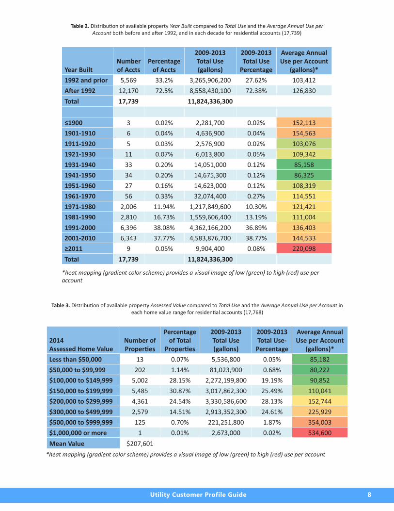
Table 2 shows the distribution of residential property year built compared to total use in terms of average annual use per account. The first two rows of the figure shows properties built before and after 1992. The significance of this date is tied to the Energy Policy Act of 1992 when there were low-use standards set for both residential and non-residential appliances, after which building codes were required to comply with the standards (Alliance for Water Efficiency, Koeller & Co, 2014). Due to this new standard, homes built after 1992 would most likely not show significant water savings from the implementation of toilet replacement and rebate programs because they already have low-flow toilets. For this reason, it is helpful to be aware of the number of properties built after the standards were set to be able to identify whether or not toilet replacement BMPs result in a large amount of savings across the entire service area, or if programs like this can be targeted at certain groups, which would require account holders to qualify for the program based on the year that the property was built.

Table 3 similarly illustrates the comparison of assessed home value to the average annual use per account. In the sample utility data set, it is clear that the average use per account increases when home value increases.

*heatmapping(gradientcolorscheme)providesavisualimageoflow(green)tohigh(red)consumptiontotalsineachclassification


2014 Assessed Home Value

Number of Properties

Percentage of Total

Properties

2009-2013 Total Use (gallons)

2009-2013 Total Use-

Percentage

Average Annual Use per Account

(gallons)*Less than $50,000 13 0.07% 5,536,800 0.05% 85,182$50,000 to $99,999 202 1.14% 81,023,900 0.68% 80,222$100,000 to $149,999 5,002 28.15% 2,272,199,800 19.19% 90,852$150,000 to $199,999 5,485 30.87% 3,017,862,300 25.49% 110,041$200,000 to $299,999 4,361 24.54% 3,330,586,600 28.13% 152,744$300,000 to $499,999 2,579 14.51% 2,913,352,300 24.61% 225,929$500,000 to $999,999 125 0.70% 221,251,800 1.87% 354,003$1,000,000 or more 1 0.01% 2,673,000 0.02% 534,600Mean Value $207,601

*heatmapping(gradientcolorscheme)providesavisualimageoflow(green)tohigh(red)useperaccount

Table 2. Distribution of available property YearBuilt compared to TotalUse and the AverageAnnualUseperAccount both before and after 1992, and in each decade for residential accounts (17,739)

Year BuiltNumber of Accts

Percentage of Accts

2009-2013 Total Use (gallons)

2009-2013 Total Use

Percentage

Average Annual Use per Account

(gallons)*1992 and prior 5,569 33.2% 3,265,906,200 27.62% 103,412After 1992 12,170 72.5% 8,558,430,100 72.38% 126,830Total 17,739 11,824,336,300

≤1900 3 0.02% 2,281,700 0.02% 152,1131901-1910 6 0.04% 4,636,900 0.04% 154,5631911-1920 5 0.03% 2,576,900 0.02% 103,0761921-1930 11 0.07% 6,013,800 0.05% 109,3421931-1940 33 0.20% 14,051,000 0.12% 85,1581941-1950 34 0.20% 14,675,300 0.12% 86,3251951-1960 27 0.16% 14,623,000 0.12% 108,3191961-1970 56 0.33% 32,074,400 0.27% 114,5511971-1980 2,006 11.94% 1,217,849,600 10.30% 121,4211981-1990 2,810 16.73% 1,559,606,400 13.19% 111,0041991-2000 6,396 38.08% 4,362,166,200 36.89% 136,4032001-2010 6,343 37.77% 4,583,876,700 38.77% 144,533≥2011 9 0.05% 9,904,400 0.08% 220,098Total 17,739 11,824,336,300

Table 3. Distribution of available property AssessedValue compared to TotalUse and the AverageAnnualUseperAccount in each home value range for residential accounts (17,768)

*heatmapping(gradientcolorscheme)providesavisualimageoflow(green)tohigh(red)useperaccount


3.2. Indoor Use compared to Outdoor Use

As described in Box 3, the winter average of all residential accounts was calculated to determine indoor use, and indoor use was subtracted from total use to determine the outdoor use for Table 4. The Summer Use table is of partic-ular interest because it fairly compares outdoor and indoor use for residential accounts in months where outdoor use is assumed to occur more frequently (summer months June to August). Although outdoor and indoor Annual Use is useful information for determining maximum use trends, it inaccurately compares the two since outdoor use does not occur year-round, whereas indoor use is assumed year-round so it shows a larger percentage of use. Figure 2 shows the summer outdoor and indoor use in graphical form.

Table 4. Assumed outdoor and indoor use totals for residential accounts (17,774)

Aggregate Assumed

DistributionAnnual Use

(gallons)

Aggregate Assumed

Distribution

Summer Use Jun-Aug (gallons) Percentage

2009 Outdoor 748,223,700 2009 Outdoor 521,371,700 55.14%2009 Indoor 1,618,737,000 2009 Indoor 424,111,400 44.86%2010 Outdoor 911,023,800 2010 Outdoor 408,263,200 55.35%2010 Indoor 1,267,888,100 2010 Indoor 329,395,600 44.65%2011 Outdoor 1,328,372,100 2011 Outdoor 679,829,400 63.83%2011 Indoor 1,500,144,300 2011 Indoor 385,196,300 36.17%2012 Outdoor 1,049,008,100 2012 Outdoor 505,920,200 60.17%2012 Indoor 1,300,963,600 2012 Indoor 334,841,900 39.83%2013 Outdoor 624,016,400 2013 Outdoor 340,739,300 46.36%2013 Indoor 1,499,686,400 2013 Indoor 394,183,300 53.64%

3.3. Cross-comparison of Indoor and Outdoor Use Levels

To categorize residential accounts into groups of similar use, consumption levels were determined using percentiles of seasonal (outdoor) and winter (indoor) use from residential consumption in 2009. For the sample data set, 2009 was used as the baseline year because it was the first year of consumption data, and it was the first year that the utility participated in conservation programming. The levels of use used for analysis are shown in Table 5.

Table 6 was determined by a cross-comparison of the use levels from ranges of use in Table 5. The first column in the figure shows the number of accounts in each group, and the second column illustrates the cumulative five-year change in number of accounts, as well as the one-year changes between each of the five years in the data set. It is desirable to see a positive change in the direction of Level 1 for both Seasonal and Winter Use, which indicates that accounts are reporting lower water consumption.


521,371,700

408,263,200

679,829,400

505,920,200

340,739,300

424,111,400

329,395,600385,196,300

334,841,900

394,183,300

945,483,100

737,658,800

1,065,025,700

840,762,100

734,922,600

0

200,000,000

400,000,000

600,000,000

800,000,000

1,000,000,000

1,200,000,000

2008 2009 2010 2011 2012 2013 2014

Summer Use (g

allons)

Consumption Year

Residential Use(June‐August, 2009‐2013; 17,774 Accounts)

Outdoor Indoor Total

Figure 2. Graphical representation of the data in Table 4; Summer Use section only

Table 5. Residential levels of use, in gallons, calculated from seasonal and winter percentiles for all accounts in 2009; seasonal and winter use is assumed to represent outdoor and indoor use,

respectively.

Monthly Consumption Levels (gallons)

LevelsSeasonal

MinSeasonal

MaxWinter

MinWinter

MaxData Set

Percentile1 0 300 1,101 3,267 10th2 301 2,742 3,268 4,542 25th3 2,743 7,367 4,543 6,400 50th4 7,368 13,933 6,401 9,367 75th5 13,934 22,633 9,368 14,100 90th6 22,634 183,467 14,101 98,333 MAX


5-Year Change 2009-20132009 Winter Winter

Levels 1 2 3 4 5 6 Levels 1 2 3 4 5 6

Seas

onal

1 149 224 348 383 280 401

Seas

onal

1 335 370 413 366 166 14

2 478 514 739 558 233 137 2 283 377 340 268 113 2

3 549 840 1257 1062 506 244 3 -6 -54 -79 24 42 -8

4 366 616 1203 1223 708 316 4 -88 -126 -402 -347 -127 -74

5 161 315 582 763 540 303 5 -29 -112 -174 -271 -169 -111

6 83 148 334 457 381 372 6 -58 -63 -173 -250 -202 -190

2010 Winter Winter

Levels 1 2 3 4 5 6 Levels 1 2 3 4 5 6

Seas

onal

1 365 461 681 704 399 255

Seas

onal

1 216 237 333 321 119 -146

2 779 929 1072 723 225 66 2 301 415 333 165 -8 -71

3 662 985 1299 948 294 82 3 113 145 42 -114 -212 -162

4 496 737 1096 828 262 79 4 130 121 -107 -395 -446 -237

5 260 378 687 494 174 66 5 99 63 105 -269 -366 -237

6 135 221 355 333 167 76 6 52 73 21 -124 -214 -296

1-YearChange2010-20112011 Winter Winter

Levels 1 2 3 4 5 6 Levels 1 2 3 4 5 6

Seas

onal

1 188 247 350 342 232 222

Seas

onal

1 -177 -214 -331 -362 -167 -33

2 424 475 597 446 170 68 2 -355 -454 -475 -277 -55 2

3 553 694 1006 761 350 144 3 -109 -291 -293 -187 56 62

4 457 739 1136 1055 488 198 4 -39 2 40 227 226 119

5 283 548 902 909 529 189 5 23 170 215 415 355 123

6 170 341 690 871 574 424 6 35 120 335 538 407 348


Levels 1 2 3 4 5 6 Levels 1 2 3 4 5 6

Seas

onal

1 321 357 515 450 237 206

Seas

onal

1 133 110 165 108 5 -16

2 676 757 846 509 169 51 2 252 282 249 63 -1 -17

3 735 960 1216 864 331 104 3 182 266 210 103 -19 -40

4 564 810 1230 934 428 114 4 107 71 94 -121 -60 -84

5 347 515 765 641 286 111 5 64 -33 -137 -268 -243 -78

6 150 282 478 436 233 146 6 -20 -59 -212 -435 -341 -278


Levels 1 2 3 4 5 6 Levels 1 2 3 4 5 6

Seas

onal

1 484 594 761 749 446 415

Seas

onal

1 163 237 246 299 209 209

2 761 891 1079 826 346 139 2 85 134 233 317 177 88

3 543 786 1178 1086 548 236 3 -192 -174 -38 222 217 132

4 278 490 801 876 581 242 4 -286 -320 -429 -58 153 128

5 132 203 408 492 371 192 5 -215 -312 -357 -149 85 81

6 25 85 161 207 179 182 6 -125 -197 -317 -229 -54 36

Table 6. NumberofAccounts, and ChangeinNumberofAccounts categorized by cross-comparison of Seasonal and Winter Use Levels

*heatmapping(gradientcolorschemes)provideavisualimageoflow(green)tohigh(red)numberofaccountsineachcategory,andanincrease(red)anddecrease(blue)innumberofaccountsbetweeneachyear


Box 5. Table Calculations: Tables 1-6

ListedbytablecolumnheadingsTimeperiodsforeachcalculationmatter–annualmeasuresunlessspecificallydesignatedby:*can be annual measure or aggregate measure of all years in the data set (as seen in the table)

Table 1 – Use Distribution: Customer Classification

Number of Accts NumberofaccountsinthedesignatedclassificationPercentage of Accts (Numberofaccountsinclassification÷Totalnumberofaccounts)x100Total Use* SumofannualuseforallaccountsinclassificationTotal Use Percentage (Sumofannualuseinclassification÷Totaluseforallaccounts)x100

Table 2 – Use Distribution: Year Built

Number of Accts NumberofaccountsinthedesignatedrangeofyearsbuiltPercentage of Accts (Numberofaccountsinyearrange÷Totalnumberofaccounts)x100Total Use* SumofannualuseforallaccountsinyearrangeTotal Use Percentage (Sumofannualuseinyearrange÷Totaluseforallaccounts)x100Avg Annual Use per Acct (Sumofannualuseinyearrange÷Numberofyearsofdata÷‘NumberofAccts’)

Table 3 – Use Distribution: Assessed Home Value

Number of Properties NumberofaccountsinthedesignatedrangeofhomevaluesPercentage of Total Properties (Numberofaccountsinhomevaluerange÷Totalnumberofaccounts)x100Total Use* SumofannualuseforallaccountsinhomevaluerangeAvg Annual Use per Acct Sumofannualuseinhomevaluerange÷Numberofyearsofdata÷‘NumberofProperties’

Table 4 – Outdoor and Indoor Use

Annual Indoor Use Annualwinteraverageforallaccountsx12[months in a year]Annual Outdoor Use Totalannualuse–‘AnnualIndoorUse’Seasonal Indoor Use Annualwinteraverageforallaccountsx3[months during summer season]Seasonal Outdoor Use SumofuseforallaccountsfromJunetoAugust–‘SeasonalIndoorUse’Percentages (AnnualIndoorUse÷TotalAnnualUse)x100

(AnnualOutdoorUse÷TotalAnnualUse)x100

Table 5 – Consumption Level Designations (use only one year of data to determine levels)

Seasonal Max Percentilesofseasonalaverageconsumption(10th,25th,50th,75th,90thandMaximumvalue)Seasonal Min Level1:Minimumseasonalaverage;Level2+:‘SeasonalMax’inLevelabove+1Winter Max Percentilesofwinteraverageconsumption(10th,25th,50th,75th,90thandMaximumvalue)Winter Min Level1:Minimumwinteraverage;Level2+:‘WinterMax’inLevelabove+1

Table 6 – Cross-comparison of Consumption Levels

Number of Accounts NumberofaccountsinagivenseasonalANDwinterconsumptionlevelChange* Changeinnumberofaccounts


Table 7, Table 8, and Table 9 report the final analysis in this phase and will help the utility determine which audience to target conservation BMPs. For all account groups that were categorized in Table 6, these tables show annual use and annual use per account for each year in the data set, and average annual use per account in the five-year period. It is evident that the account group in level 4 of both seasonal and winter use tends to show the largest total use in Table 7 and Table 9. This group represents the largest user of water within the residential classification, and the character-istics of this group can be evaluated from the integrated consumption and property data set to determine which BMP will best encourage the group to reduce their consumption. There also exists an opportunity to target BMPs toward level 10 of both seasonal and winter use with the largest annual use per account, as seen in Table 8 and Table 9. This group has different characteristics from those in level 10, so conservation programming may be determined to best target those account holders.

In addition, Table 8 and Table 9 show a baseline metric (blue line) that can be considered a defining level of efficient consumption, in the sample utility service area, where it is desirable for a larger number of accounts to stay below. Individual utility baseline metrics are calculated using the number of persons per household, which is determined on an individual service area basis (U.S. Census Bureau, 2015), and the national median indoor use per person, 60 gpcd, determined by a residential water use study funded by the Water Research Foundation (Mayer, et al., 1999). Table 8 also offers an actual annual indoor use metric (red line) in order to compare actual to desired consumption and is calculated using the average of the winter average of each account in the consumption data set.

Recommendations

Frequency of Analysis

It is important for the process of utility customer characterization to occur on a regular basis. Annual customer characterizations within the utility or utility conservation program will produce more accurate and informative trends of water consumption within different customer categories. Managers will become familiar with normal usage trends and be able to better recognize anomalous and consistent high consumption levels. An annual process will also help managers target BMPs accordingly and to be able to recognize the point at which specific BMPs are no longer needed among different groups, when accompanied with program evaluations.

Outliers, or customers with significantly higher annual consumption than other similar users in their category, may be apparent and indicate the need for inquiry. Additionally, if a customer has a significant increase in annual consump-tion, an examination would benefit both the customer and the utility. If customers have unusually high consumption as a result of inefficient practices, the utility has an opportunity to work with that user to reduce consumption.

Computational Assistance

Where utility and conservation managers benefit from being able to look at data trends, they may also benefit from computational assistance within Information Technology and GIS departments. Those technicians trained in data manipulation and analysis may be able to more efficiently prepare and sort data sets, and present them in a way that is useful to managers for making decisions about conservation programming.

BMP Selection

Once the characteristics of high consumptive users have been identified, BMPs may be chosen. When considering conservation programs for residential customers, indoor and outdoor programs are usually separated, focusing more heavily on indoor programming since making changes to fixtures and appliances inside the home makes it easier for customers to participate, rather than making changes in water use behavior. For example, it is common for utilities to adopt toilet replacement programs early in the planning process because low-flow toilets save a considerable amount of water when replacing older high-flow toilets.


2009 Winter

Levels 1 2 3 4 5 6

Seas

onal

1 4,667,400 9,915,900 21,059,800 30,857,100 31,202,600 78,958,900

2 30,296,300 28,264,100 53,387,500 53,585,800 30,283,400 28,158,900

3 30,047,000 59,356,300 109,990,400 118,632,300 75,135,600 54,706,700

4 29,508,600 58,129,500 134,664,600 166,685,100 120,909,300 78,967,100

5 18,717,200 41,203,800 85,205,600 127,335,600 110,520,300 85,754,700

6 15,906,200 28,612,000 70,197,800 107,982,400 105,258,800 144,429,200

2010 Winter

Levels 1 2 3 4 5 6

Seas

onal

1 11,714,800 21,467,400 41,328,400 59,565,500 44,718,600 45,661,000

2 32,714,000 53,803,700 80,189,400 72,243,200 30,888,200 13,588,400

3 41,996,300 77,457,200 124,883,600 116,394,100 46,845,800 18,196,000

4 49,021,900 84,572,000 144,122,200 130,550,600 51,893,500 21,832,600

5 37,801,900 60,884,600 123,867,300 100,825,900 43,412,000 21,213,100

6 30,725,700 55,113,700 93,419,600 99,802,100 59,656,700 36,464,100

2011 Winter

Levels 1 2 3 4 5 6

Seas

onal

1 6,044,300 11,115,200 21,586,800 27,891,600 25,734,500 41,370,800

2 17,703,800 27,144,800 44,281,200 44,546,800 23,014,100 14,928,100

3 34,826,200 52,834,300 94,666,100 90,739,800 54,683,600 33,948,200

4 43,054,400 79,628,200 143,786,300 159,745,200 93,143,600 54,383,200

5 39,000,600 84,638,900 154,995,100 178,676,600 125,043,700 60,183,300

6 37,530,700 80,107,800 179,913,500 253,485,400 196,470,400 197,493,700

2012 Winter

Levels 1 2 3 4 5 6

Seas

onal

1 9,877,600 16,017,100 31,210,100 37,247,900 25,818,100 37,379,400

2 26,694,100 42,297,000 61,631,500 50,344,600 22,864,400 11,262,900

3 43,797,100 71,894,600 113,267,000 103,251,400 52,901,000 25,108,000

4 53,566,100 90,218,500 158,021,200 145,943,400 83,193,700 31,118,900

5 48,899,600 82,167,000 135,471,000 128,993,700 68,942,000 37,105,600

6 33,059,100 68,129,200 126,606,500 126,310,000 81,294,200 68,068,200

2013 Winter

Levels 1 2 3 4 5 6

Seas

onal

1 14,400,900 26,678,900 45,294,100 60,124,200 47,914,500 82,645,500

2 29,985,900 49,557,600 78,222,400 79,672,800 46,230,300 31,522,800

3 31,871,100 58,116,100 107,236,700 126,380,500 83,996,100 53,928,300

4 24,881,300 50,992,100 97,072,500 130,092,700 107,181,000 64,924,700

5 17,296,800 29,781,600 67,667,200 92,881,600 82,806,100 57,714,500

6 5,050,700 18,129,200 38,515,200 54,879,000 55,328,300 74,695,100

Table 7. AnnualUse (gallons) for residential accounts in Table 6

*heatmapping(gradientcolorscheme)providesavisualimageoflow(green)tohigh(red)con-sumptiontotalsineachcategory


Baseline (blue line): 2.96 pphh * 60 gpcd * 365 d/yr = 64,824 gal/acct/year

2009 Winter

Levels 1 2 3 4 5 6

Seas

onal

1 31,325 44,267 60,517 80,567 111,438 196,905

2 63,381 54,989 72,243 96,032 129,972 205,539

3 54,730 70,662 87,502 111,706 148,489 224,208

4 80,625 94,366 111,941 136,292 170,776 249,896

5 116,256 130,806 146,401 166,888 204,667 283,019

6 191,641 193,324 210,173 236,285 276,270 388,251

Actual Average Indoor Use: 7,954 gal/acct/m * 12 m/yr = 95,445 gal/acct/yr

2010 Winter

Levels 1 2 3 4 5 6

Seas

onal

1 32,095 46,567 60,688 84,610 112,077 179,063

2 41,995 57,916 74,804 99,921 137,281 205,885

3 63,439 78,637 96,138 122,779 159,339 221,902

4 98,834 114,752 131,498 157,670 198,067 276,362

5 145,392 161,070 180,302 204,101 249,494 321,411

6 227,598 249,383 263,154 299,706 357,226 479,791


2011 Winter

Levels 1 2 3 4 5 6

Seas

onal

1 32,151 45,001 61,677 81,554 110,925 186,355

2 41,754 57,147 74,173 99,881 135,377 219,531

3 62,977 76,130 94,101 119,238 156,239 235,751

4 94,211 107,751 126,572 151,417 190,868 274,663

5 137,811 154,451 171,835 196,564 236,378 318,430

6 220,769 234,920 260,744 291,028 342,283 465,787


2012 Winter

Levels 1 2 3 4 5 6

Seas

onal

1 30,771 44,866 60,602 82,773 108,937 181,453

2 39,488 55,875 72,850 98,909 135,292 220,841

3 59,588 74,890 93,147 119,504 159,822 241,423

4 94,975 111,381 128,473 156,256 194,378 272,973

5 140,921 159,548 177,086 201,238 241,056 334,285

6 220,394 241,593 264,867 289,702 348,902 466,221


2013 Winter

Levels 1 2 3 4 5 6

Seas

onal

1 29,754 44,914 59,519 80,273 107,432 199,146

2 39,403 55,620 72,495 96,456 133,614 226,783

3 58,694 73,939 91,033 116,372 153,278 228,510

4 89,501 104,066 121,189 148,508 184,477 268,284

5 131,036 146,707 165,851 188,784 223,197 300,596

6 202,028 213,285 239,225 265,116 309,097 410,413

Actual Average Annual Use: 7,393 gal/acct/m * 12 m/yr = 88,710 gal/acct/yr

Table 8. AnnualUseperAccount (gallons) for residential accounts in Table 6


However, as mentioned in the Table 2 discussion, the Energy Policy Act of 1992 passed national efficiency standards stating that toilets were not allowed to be installed in new development if they did not meet a 1.6 gallon per flush or less requirement. As a result, manufacturers no longer produce toilets with flow rates higher than 1.6 gallons per flush, and all development is required to meet this standard. Thus, the customer characterization is important in identifying whether or not a toilet replacement program would result in water savings at a reasonable cost to the utility.

Aggregate 5-Year Use Winter

Levels 1 2 3 4 5 6Se

ason

al

1 46,705,000 85,194,500 160,479,200 215,686,300 175,388,300 286,015,600

2 137,394,100 201,067,200 317,712,000 300,393,200 153,280,400 99,461,100

3 182,537,700 319,658,500 550,043,800 555,398,100 313,562,100 185,887,200

4 200,032,300 363,540,300 677,666,800 733,017,000 456,321,100 251,226,500

5 161,716,100 298,675,900 567,206,200 628,713,400 430,724,100 261,971,200

6 122,272,400 250,091,900 508,652,600 642,458,900 498,008,400 521,150,300

*heatmapping(gradientcolorscheme)providesavisualimageoflow(green)tohigh(red)consumptiontotalsineachcategory

Average Annual Use per Account (over 5-year period) Winter

Levels 1 2 3 4 5 6

Seas

onal

1 31,219 45,123 60,600 81,955 110,162 188,584

2 45,204 56,309 73,313 98,240 134,307 215,716

3 59,886 74,852 92,384 117,920 155,433 230,359

4 91,629 106,463 123,935 150,029 187,713 268,435

5 134,283 150,516 168,295 191,515 230,958 311,548

6 212,486 226,501 247,633 276,367 326,755 442,092

Baseline (blue line): 2.96 pphh * 60 gpcd * 365 d/yr = 64,824 gal/acct/year

Table 9. AggregateUseand AverageAnnualUseperAccountin five years (gallons) for residential accounts in Table 6

Box 6. Table Calculations: Tables 7-9

Table 7 – Annual Use (1-Year Periods)

Annual Use SumofuseforallaccountsinagivenseasonalANDwinterconsumptionlevelforthegivenyear

Table 8 – Annual Use Per Account (1-Year Periods)

Annual Use per Acct ‘AnnualUse’inlevel[Table 7. ÷Numberofaccountsinlevel[Table 6.]Baseline (blue line) Personsperhouseholdx60gallons/person/dayx365days/yearActual Avg Indoor Use (red line) UtilityAnnualWinterAveragex12months/year

Table 9. – Aggregate Use and Average Annual Use Per Account (5-Year Period)

Aggregate Use Sumof‘AnnualUse’inlevel[Table 7]Avg. Annual Use per Acct Averageofthe‘AnnualUseperAcct’inallyears[Table 8]Baseline (blue line) Personsperhouseholdx60gallons/person/dayx365days/year


NationalEfficiencyStandardsandSpecifications

Along with standards for water use in toilet fixtures, the Alliance for Water Efficiency publishes an updated matrix, most recently the 2014 National Efficiency Standards and Specifications for Residential and Commercial Water-Us-ing Fixtures and Appliances, which outlines efficient standards for all residential and commercial fixtures and appli-ances in terms of the Energy Policy Act of 1992, the U.S. Environmental Protection Agency “WaterSense” program, and the Consortium for Energy Efficiency (Alliance for Water Efficiency, Koeller & Co, 2014).

NorthAmericanIndustrialClassificationSystem

As mentioned in Phase II – Preparing Data, the North American Industrial Classification System (NAICS) is a helpful way to standardize the categorization of non-residential customers (U.S. Census Bureau, 2014). The City of Garland, Texas was recently cited in a presentation given by the Texas Water Development Board as identifying an existing, unused field within their billing system that they were able to utilize to input the six-digit NAICS code for each non-residential customer (Kluge, 2015). This standardization will make it easier and faster for the utility to create a consistent customer characterization.

Program Evaluation

The best way to ensure that chosen conservation BMPs are continuing to be successful in reducing consumption and continue to target the correct audience is to conduct BMP evaluations before and after implementation, in addition to an annual customer characterization. Consistent program evaluations will indicate when a BMP is no longer produc-ing a significant amount of water savings, and will give the utility an opportunity to make adjustments.

Maintain Relationships

Successful water conservation planning requires a cooperative culture from all groups of home and business owners in the utility service area. Maintaining positive relationships with local landscape companies, building management companies, and homeowners associations will help establish buy-in for conservation programs and the positive promotion of associated BMPs.

Transient Populations

When engaging in water conservation planning, it is helpful to be aware that customers affiliated with a large military or higher education presence, referred to as transient populations, will make conservation efforts challenging to implement. Transient populations introduce a higher rate of turnover in customers that are sometimes new to the geographic region, and therefore unfamiliar with existing conservation efforts. As a result, transient populations require a higher rate of education and outreach programs.

Conclusion

Adopting the customer characterization process outlined in this document, or a similar process, will make targeted conservation programming easier and quicker to achieve. This familiarity with the customer base will also allow the utility to leverage available resources to their fullest potential, realize the greatest water savings at the least cost.


References

Alliance for Water Efficiency, Koeller & Co. (2014, March 21). NationalEfficiencyStandardsandSpecificationsforResiden-tialandCommercialWater-UsingFixturesandAppliances. Retrieved December 2014, from Alliance for Water Efficiency - Standards & Codes for Water Efficiency: http://www.allianceforwaterefficiency.org/Codes_and_Standards_Home_Page.aspx

Brehe, T. A., and Coll, E. (2012). A Disruptive Innovation That Will Transform Water Conservation Performance. Journal-AmericanWaterWorksAssociation,104(10), 60-63.

Kluge, K. (2015, January 30). UtilityEvaluationforConservationPlanning[Webinar]. Retrieved from The Texas Water Conservation Series: http://www.tawwa.org/?page=2015watercon

Mayer, P. W., DeOreo, W. B., Opitz, E. M., Jack C. Kiefer, W. Y., Dziegielewski, B., and Nelson, J. O. (1999). ResidentialEndUsesofWater. Denver: AWWA Research Foundation and American Water Works Association.

Morales, M. A., and Heaney, J. P. (2014). Classification, Benchmarking, and Hydroeconomic Modeling of Nonresidential Water Users. Journal-AmericanWaterWorksAssociation,106(12), E550-560.

U.S. Census Bureau. (2010). CommunityFacts. Retrieved November 2014, from American FactFinder: http://factfinder2.census.gov/faces/nav/jsf/pages/index.xhtml

U.S. Census Bureau. (2014, November 5). NorthAmericanIndustryClassificationSystem. Retrieved December 2014, from United States Census Bureau: http://www.census.gov/eos/www/naics/

U.S. Census Bureau. (2015). QuickFactsBeta. Retrieved February 2015, from United States Census Bureau: http://www.census.gov/quickfacts/table/PST045214/00

Vickers, A., Tiger, M. W., and Eskaf, S. (2013, October). AGuidetoCustomerWater-UseIndicatorsforConservationandFinancialPlanning. American Water Works Association.

http://www.allianceforwaterefficiency.org/Codes_and_Standards_Home_Page.aspx

http://www.allianceforwaterefficiency.org/Codes_and_Standards_Home_Page.aspx

http://www.tawwa.org/?page=2015watercon

http://factfinder2.census.gov/faces/nav/jsf/pages/index.xhtml

http://factfinder2.census.gov/faces/nav/jsf/pages/index.xhtml

http://www.census.gov/eos/www/naics/

http://www.census.gov/quickfacts/table/PST045214/00

http://www.census.gov/quickfacts/table/PST045214/00


Phase I – Gather Data

Data needed for process • Billed consumption data • Property data

Other helpful data • US Census Bureau databases • Geographical information system (GIS) spatial data

Phase II – Clean Data

Prepare data set • Save all data in separate spreadsheet for recovery purposes • Optional - Format data into a table for easier sorting and management

(‘Format as Table’ function in Excel)

Identify all monthly consumption data for complete years • Retain only data reported for the desired year range (complete year - December of one year to December of the next year)

Identify units of monthly billed consumption • Common units are gallons or thousand gallons

Remove closed accounts • Identify a service status that indicates if the account is open or closed (designated by the utility, not assumed)

Create columns for calculating annual metrics • Annual Total • Annual Winter (Indoor) Average • Annual Seasonal Average • Annual Assumed Outdoor Use

Separate residential and non-residential classification data

Remove low-use accounts for all monthly consumption data • Low-use threshold: < 1,000 gallons per month

Create columns for importing property information • A unique identifier for each account • Year Built • Most recent Assessed Property Value

Import property data from Appraisal District database • Import unique identifiers • Import years built • Import most recent assessed home values

(‘VLOOKUP’ formula in Excel)

Examine accounts without individual unique identifiers • Typos and abbreviations can interfere with the import of property data

Phase III – Analyze Data

Create use distributions • Customer Classification • Property Year Built • Assessed Home Value

Compare indoor and outdoor Use

Cross-compare indoor and outdoor percentiles • Categories of similar indoor and outdoor use

• Identify column containing customer classifications (designated by the utility, not assumed)

Appendix A: Customer Profile Process Chart

Utility Customer Profile Guide

utility customer profile guide for water conservation...

Documents