using tabu search to configure support vector regression ... · using tabu search to configure...
TRANSCRIPT
Using tabu search to configure support vector regressionfor effort estimation
A. Corazza & S. Di Martino & F. Ferrucci & C. Gravino &
F. Sarro & E. Mendes
# Springer Science+Business Media, LLC 2011Editor: Tim Menzies and Gunes Koru
Abstract Recent studies have reported that Support Vector Regression (SVR) has thepotential as a technique for software development effort estimation. However, its predictionaccuracy is heavily influenced by the setting of parameters that needs to be done whenemploying it. No general guidelines are available to select these parameters, whose choicealso depends on the characteristics of the dataset being used. This motivated the workdescribed in (Corazza et al. 2010), extended herein. In order to automatically select suitableSVR parameters we proposed an approach based on the use of the meta-heuristics TabuSearch (TS). We designed TS to search for the parameters of both the support vectoralgorithm and of the employed kernel function, namely RBF. We empirically assessed theeffectiveness of the approach using different types of datasets (single and cross-companydatasets, Web and not Web projects) from the PROMISE repository and from the Tukutuku
Empir Software EngDOI 10.1007/s10664-011-9187-3
A. Corazza : S. Di MartinoUniversity of Napoli “Federico II”, Via Cintia, 80126 Naples, Italy
A. Corazzae-mail: [email protected]
S. Di Martinoe-mail: [email protected]
F. Ferrucci (*) : C. Gravino : F. SarroUniversity of Salerno, Via Ponte don Melillo, 84084 Fisciano (SA), Italye-mail: [email protected]
F.. Ferruccie-mail: [email protected]
C. Gravinoe-mail: [email protected]
F. Sarroe-mail: [email protected]
E. MendesZayed University, P.O. Box 18292, Dubai, UAEe-mail: [email protected]
database. A total of 21 datasets were employed to perform a 10-fold or a leave-one-outcross-validation, depending on the size of the dataset. Several benchmarks were taken intoaccount to assess both the effectiveness of TS to set SVR parameters and the predictionaccuracy of the proposed approach with respect to widely used effort estimation techniques.The use of TS allowed us to automatically obtain suitable parameters’ choices required torun SVR. Moreover, the combination of TS and SVR significantly outperformed all theother techniques. The proposed approach represents a suitable technique for softwaredevelopment effort estimation.
Keywords Effort estimation . Search based techniques . Support vector regression . Tabusearch
1 Introduction
Early estimation of software development effort is a critical management activity. Indeed,realistic estimates are crucial to the adequate allocation of resources and also affect thecompetitiveness of a software company (Mendes 2009). Several studies have addressed thisproblem (e.g., Briand et al. 1999; Briand et al. 2000; Briand and Wieczorek 2002;Costagliola et al. 2006; Maxwell et al. 1999; Mendes et al. 2003b; Shepperd et al. 1996;Shepperd and Schofield 1997), many of which focusing on the proposal and evaluation oftechniques to construct predictive models able to estimate the effort of a new projectexploiting information (actual effort and cost-drivers) related to past projects. In particular,recent studies (Corazza et al. 2009, 2010, 2011) have investigated the effectiveness ofSupport Vector Regression (SVR) for software effort estimation. SVR is a technique basedon Support Vector Machines, a family of Machine Learning algorithms that have beensuccessfully applied for addressing several predictive data modeling problems (Cristianiniand Shawe-Taylor 2000; Smola and Schölkopf 2004). The studies reported in (Corazza etal. 2009, 2011) showed that SVR has potential use also for software development effortestimation; indeed it outperformed the most commonly adopted prediction techniques usingthe Tukutuku database (Mendes et al. 2005a, b), a cross-company dataset of Web projectswidely adopted in Web effort estimation studies. It was argued that the main reason for thatlies in the flexibility of the method. Indeed, SVR enables the use of kernels and parametersettings allowing the learning mechanism to better suit the characteristics of differentchunks of data, which is a typical characteristic of cross-company datasets. However, thesetting of parameters needs to be done carefully, since an inappropriate choice can lead toover- or under-fitting, heavily worsening the performance of the method (Chang and Lin2001; Keerthi 2002). Nevertheless, there are no guidelines on how to best select theseparameters (Scholkopf and Smola 2002; Vapnik and Chervonenkis 1964; Vapnik 1995)since the appropriate setting depends on the characteristics of the employed dataset.Moreover, an examination of all possible values for parameters is not computationallyaffordable, as the search space is too large, also due to the interaction among parameters,which cannot be separately optimized.
The issues abovementioned have motivated us to investigate the use of Tabu Search (TS)to automatically select SVR parameters (Corazza et al. 2010). TS is a meta-heuristic searchtechnique used to address several optimization problems (Glover and Laguna 1997). TheTS-based approach was first investigated in (Corazza et al. 2010) employing SVR incombination with different kernels and variables’ preprocessing strategies, using as datasetthe Tukutuku database (Mendes et al. 2005a). In particular, we compared SVR configured
Empir Software Eng
with TS (SVR + TS) with other effort estimation techniques, namely Manual StepWiseRegression (MSWR), Case-Based Reasoning (CBR), Bayesian Networks (Mendes 2008),and the Mean and Median effort of the training sets. SVR + TS gave us the best results everachieved with the Tukutuku database. However, these results were based on two randomsplits of only one cross-company dataset and it is widely recognized that several empiricalanalysis are needed to generalize empirical findings. Thus, the aim of this paper is to furtherinvestigate the combination of TS and SVR using data from several single- and cross-company datasets. Let us recall that the former represents a dataset containing data onprojects from a single software company while the latter includes project data gathered fromseveral software companies. In our analysis, we employed 13 different datasets from thePROMISE repository and also other 8 datasets obtained by splitting the Tukutuku databaseaccording to the values of its four categorical variables (see Appendix A). The choice to usedatasets from the PROMISE repository is motivated due to the following points:
– Availability of datasets on industrial software projects, representing a diversity ofapplication domains and projects’ characteristics. This is also in line with recommen-dation made by Kitchenham and Mendes (2009).
– Availability of projects that are not Web-based, thus enabling the assessment of theeffectiveness of the estimation technique employed herein when applied to differenttypes of applications – Web, using the Tukutuku, and non-Web, using the PROMISEdatasets. We would also like to point out that, in our view, Web and softwaredevelopment differ in a number of areas, such as: application characteristics, primarytechnologies used, approach to quality delivered, development process drivers,availability of the application, customers (stakeholders), update rate (maintenancecycles), people involved in development, architecture and network, disciplinesinvolved, legal, social, and ethical issues, and information structuring and design. Adetailed discussion on this issue is provided in (Mendes et al. 2005b).
– Availability of single- and cross-company datasets, thus enabling the assessment of theestimation technique employed herein when applied to single- and cross-companydatasets. We would also like to point out that the use of a cross-company dataset isparticularly useful for companies that do not have their own data on past projects fromwhich to obtain their estimates, or that have data on projects developed in differentapplication domains and/or technologies. To date, several studies have investigated ifestimates obtained using cross-company datasets can be as accurate as the ones obtainedusing single-company datasets (e.g., Briand et al. 1999; Jeffery et al. 2000; Kitchenhamand Mendes 2004; Corazza et al. 2010; Lefley and Shepperd 2003; Maxwell et al. 1999;Mendes et al. 2008; Mendes and Kitchenham 2004; Wieczorek and Ruhe 2002)achieving different findings (see Kitchenham et al. 2007 for a systematic review).
In relation to the choice of SVR kernels and pre-processing strategies, we focused ouranalysis on the RBF kernel and a logarithmic transformation of the variables since theyprovided the best results in our previous study (Corazza et al. 2010).
In order to verify whether the proposed TS technique is able to make a suitable choice ofSVR parameters we also compared the estimates obtained with SVR + TS with thoseobtained applying SVR using different strategies for parameters selection, namely:
– random SVR configurations. This means that the same number of solutionsinvestigated for SVR + TS was generated in a totally random fashion and the bestone among them was selected according to the same criteria employed for SVR + TS.This is a natural benchmark when using meta-heuristic search techniques;
Empir Software Eng
– default parameters employed by the Weka tool (Hall et al. 2009);– the Grid-search algorithm provided by (Chang and Lin 2001).
In addition, we also assessed whether the estimates provided by the proposed approachwere better than those obtained using the Mean and Median effort (popular and simplebenchmarks for effort estimation techniques) and those achieved with MSWR and CBR.These techniques were chosen because they are the two techniques widely used in theliterature and also in industry, and the mostly employed estimation techniques (Mair andShepperd 2005).
Consequently, the research questions addressed in this paper are:
RQ1. Is Tabu Search able to effectively set Support Vector Regression parameters?RQ2. Are the effort predictions obtained by using Support Vector Regression configured
with Tabu Search significantly superior to the ones obtained by other techniques?
The remainder of the paper is organized as follows. Section 2 first reports on the mainaspects of SVR and TS and then describes the proposed approach based on TS to set-upSVR parameters. Section 3 presents the design of our empirical study, i.e., the datasets, thenull hypotheses, the validation method, and the evaluation criteria employed to assess theprediction accuracy. Results are presented in Section 4, followed by a discussion on theempirical study validity in Section 5. Related work is discussed in Section 6. Final remarksand some future work conclude the paper.
2 Using Support Vector Regression in Combination with Tabu Search for EffortEstimation
In this section, we describe Support Vector Regression, Tabu Search, and how we havecombined them for effort estimation.
2.1 Support Vector Regression
Support Vector Regression is a regression technique based on Support Vector (SV)machines, a learning approach originally introduced for linear binary classification. Linearclassifiers construct a hyperplane separating the training set points belonging to the twoclasses. In the SV machine classifier (Vapnik and Chervonenkis 1974; Vapnik 1995), thehyperplane maximizes the classification margin, that is the minimum distance of thehyperplane from the training points (Vapnik and Chervonenkis 1974), as shown in Fig. 1.Choosing such optimal hyperplane requires the solution of a quadratic optimizationproblem subject to linear constraints, corresponding to the fact that each point of thetraining set must be correctly labeled. The hyperplane resulting from this optimization onlydepends on a subset of the training points, called support vectors. As an example, in Fig. 1the three points closest to the classification hyperplane are highlighted, as they represent thesupport vectors.
Thus, the system admits a solution only if there is a hyperplane separating the twoclasses in the training set (as in Fig. 1), i.e., when the training set is linearly separable.Nevertheless, this can be considered too restrictive to be of any practical interest. Thus, in1995, Cortes and Vapnik (1995) defined a modified version of the approach, by introducinga parameter C to allow (but penalize) misclassifications in the training set, thus obtainingsoft margin SVM’s. The choice of the best value for C is crucial to performance, as it
Empir Software Eng
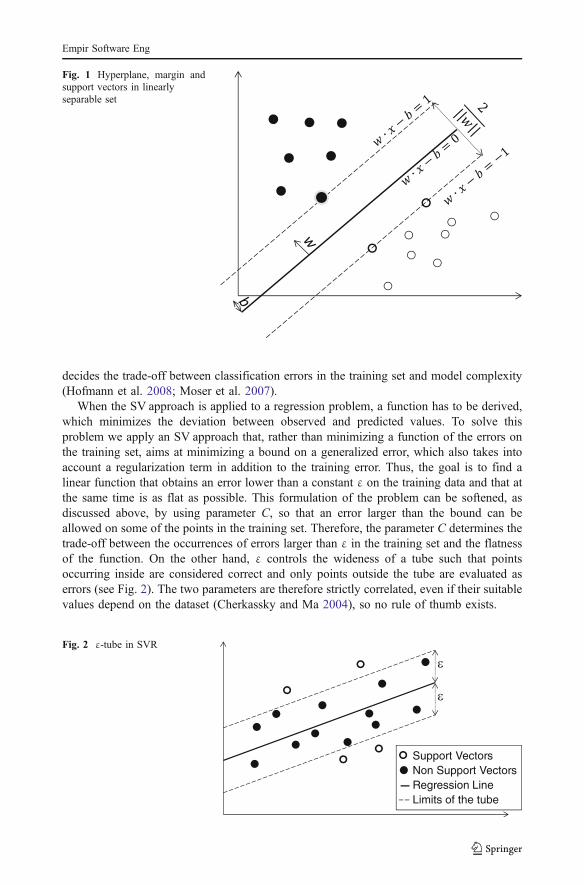
decides the trade-off between classification errors in the training set and model complexity(Hofmann et al. 2008; Moser et al. 2007).
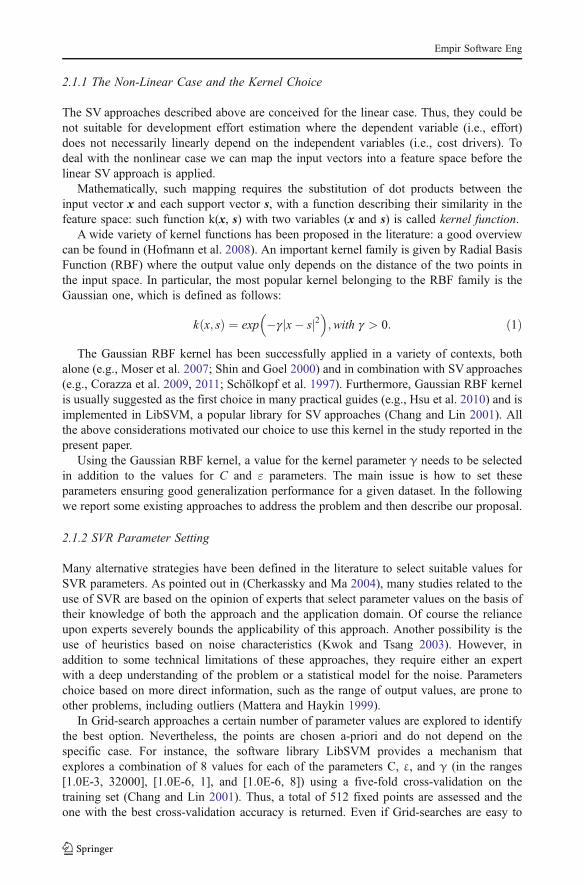
When the SV approach is applied to a regression problem, a function has to be derived,which minimizes the deviation between observed and predicted values. To solve thisproblem we apply an SV approach that, rather than minimizing a function of the errors onthe training set, aims at minimizing a bound on a generalized error, which also takes intoaccount a regularization term in addition to the training error. Thus, the goal is to find alinear function that obtains an error lower than a constant ε on the training data and that atthe same time is as flat as possible. This formulation of the problem can be softened, asdiscussed above, by using parameter C, so that an error larger than the bound can beallowed on some of the points in the training set. Therefore, the parameter C determines thetrade-off between the occurrences of errors larger than ε in the training set and the flatnessof the function. On the other hand, ε controls the wideness of a tube such that pointsoccurring inside are considered correct and only points outside the tube are evaluated aserrors (see Fig. 2). The two parameters are therefore strictly correlated, even if their suitablevalues depend on the dataset (Cherkassky and Ma 2004), so no rule of thumb exists.
Support VectorsNon Support VectorsRegression LineLimits of the tube
Fig. 2 ε-tube in SVR
Fig. 1 Hyperplane, margin andsupport vectors in linearlyseparable set
Empir Software Eng
2.1.1 The Non-Linear Case and the Kernel Choice
The SV approaches described above are conceived for the linear case. Thus, they could benot suitable for development effort estimation where the dependent variable (i.e., effort)does not necessarily linearly depend on the independent variables (i.e., cost drivers). Todeal with the nonlinear case we can map the input vectors into a feature space before thelinear SV approach is applied.
Mathematically, such mapping requires the substitution of dot products between theinput vector x and each support vector s, with a function describing their similarity in thefeature space: such function k(x, s) with two variables (x and s) is called kernel function.
A wide variety of kernel functions has been proposed in the literature: a good overviewcan be found in (Hofmann et al. 2008). An important kernel family is given by Radial BasisFunction (RBF) where the output value only depends on the distance of the two points inthe input space. In particular, the most popular kernel belonging to the RBF family is theGaussian one, which is defined as follows:
k x; sð Þ ¼ exp g x sj j2
;with g > 0: ð1Þ
The Gaussian RBF kernel has been successfully applied in a variety of contexts, bothalone (e.g., Moser et al. 2007; Shin and Goel 2000) and in combination with SVapproaches(e.g., Corazza et al. 2009, 2011; Schölkopf et al. 1997). Furthermore, Gaussian RBF kernelis usually suggested as the first choice in many practical guides (e.g., Hsu et al. 2010) and isimplemented in LibSVM, a popular library for SV approaches (Chang and Lin 2001). Allthe above considerations motivated our choice to use this kernel in the study reported in thepresent paper.
Using the Gaussian RBF kernel, a value for the kernel parameter γ needs to be selectedin addition to the values for C and ε parameters. The main issue is how to set theseparameters ensuring good generalization performance for a given dataset. In the followingwe report some existing approaches to address the problem and then describe our proposal.
2.1.2 SVR Parameter Setting
Many alternative strategies have been defined in the literature to select suitable values forSVR parameters. As pointed out in (Cherkassky and Ma 2004), many studies related to theuse of SVR are based on the opinion of experts that select parameter values on the basis oftheir knowledge of both the approach and the application domain. Of course the relianceupon experts severely bounds the applicability of this approach. Another possibility is theuse of heuristics based on noise characteristics (Kwok and Tsang 2003). However, inaddition to some technical limitations of these approaches, they require either an expertwith a deep understanding of the problem or a statistical model for the noise. Parameterschoice based on more direct information, such as the range of output values, are prone toother problems, including outliers (Mattera and Haykin 1999).
In Grid-search approaches a certain number of parameter values are explored to identifythe best option. Nevertheless, the points are chosen a-priori and do not depend on thespecific case. For instance, the software library LibSVM provides a mechanism thatexplores a combination of 8 values for each of the parameters C, ε, and γ (in the ranges[1.0E-3, 32000], [1.0E-6, 1], and [1.0E-6, 8]) using a five-fold cross-validation on thetraining set (Chang and Lin 2001). Thus, a total of 512 fixed points are assessed and theone with the best cross-validation accuracy is returned. Even if Grid-searches are easy to
Empir Software Eng
apply, they have a main drawback: the search is performed always on the same (coarsegrained) points, without taking into account the dataset to guide the search.
In (Corazza et al. 2009, 2011) the problem was addressed in the context of effortestimation, adopting an automatic approach to explore a large number of parameter values(employing various nested cycles with small incremental steps). For each run, depending onthe kernel, the number of executions ranged from some dozens to more than 4000executions. An inner leave-one-out cross validation was performed on the training set (eachcycle of execution required a number of iterations corresponding to the cardinality of thetraining set) and for each iteration the goodness of the solution was evaluated using acombination of effort accuracy estimation measures 1. Thus, the setting providing the bestestimation (according to the selected criterion) on the training set was chosen.
Although such optimization strategy included a quite large combination of parametervalues, it proceeded by brute force, by predefined steps, and did not use any informationrelated to the prior steps trying to improve the search. Moreover, it was computationally tooexpensive. Smarter optimization strategies, on the contrary, use all possible clues to focusthe search in the most promising areas of parameter values for a given dataset. Among suchstrategies, in (Corazza et al. 2010) we proposed the use of the meta-heuristics Tabu Searchto search for the best parameter settings. This approach is further investigated in this paperand will be described in the next section. One of the strengths of the Tabu Search strategy isthat it uses information both in a positive way, to focus the search, and in a negative way, toavoid already explored areas and loops.
2.2 Tabu Search
Tabu Search (TS) is a meta-heuristic search algorithm that can be used for solvingoptimization problems. The method was proposed originally by Glover to overcome somelimitations of Local Search (LS) heuristics (Glover and Laguna 1997). Indeed, whileclassical LS heuristics at each iteration constructs from a current solution i a next solution jand checks whether j is worse than i to determine if the search has to be stopped, a TSoptimization step consists in creating from a current solution i a set of solutions N(i) (alsocalled neighboring solutions) and selecting the best available one to continue the search. Inparticular, TS usually starts with a random solution and applies local transformations (i.e.,moves) to the current solution i to create N(i). When no improving neighboring solutionexists, TS allows for a climbing move, i.e., a temporary worsening move can be performed.The search terminates when a stopping condition is met (e.g., a maximum number ofiteration is reached). To determine whether a solution is worse (or better) than another anobjective function is employed. In order to prevent loops and to guide the search far fromalready visited portions of the search space, some moves can be classified as tabu whichmeans that are forbidden. The tabu moves can be stored in a list, named Tabu List, of fixedor variable length following a short-term (i.e., moves leading to already visited solutions arestored) or a long-term memory strategy (i.e., moves that have been performed several timesare stored). Since tabu moves sometimes may prohibit attractive solutions or may lead to anoverall stagnation of the searching process (Glover and Laguna 1997), the so calledaspiration criteria can be used to revoke the tabu status of a move. A common aspirationcriterion allows for a tabu move if it results in a solution which has an objective value betterthan the current solution.
1 The same combination of effort estimation measures is used as objective function in the present paper, so itwill be detailed in Section 2.3.
Empir Software Eng
To summarize, TS starting from a random solution, at each iteration explores a searchspace consisting of a set of moves. Such moves are often local transformations of thecurrent solution and depend on the problem to be solved. Among these moves, the one thatprovides the best objective value and is not tabu or matches an aspiration criterion isselected to continue the search.
Thus, to tailor the TS meta-heuristics to a given problem we have to perform thefollowing choices:
– define a representation of possible solutions and the way for generating the initial one;– define local transformations (i.e., moves) to be applied to the current solution for
exploring the neighbor solutions;– choose a means to evaluate the neighborhood (i.e., an objective function), thus guiding
the search in a suitable way;– define the Tabu list, the aspiration criteria, and the termination criteria.
In the next section we describe how we designed TS for setting SVR parameters, thusspecifying the above choices.
2.3 Using Tabu Search to Configure SVR
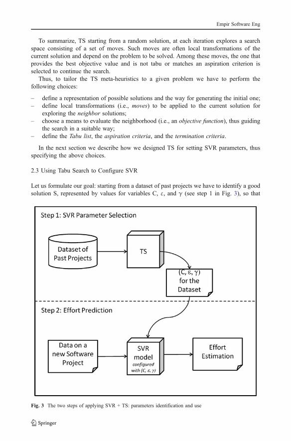
Let us formulate our goal: starting from a dataset of past projects we have to identify a goodsolution S, represented by values for variables C, ε, and γ (see step 1 in Fig. 3), so that
Fig. 3 The two steps of applying SVR + TS: parameters identification and use
Empir Software Eng
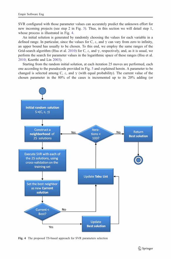
SVR configured with those parameter values can accurately predict the unknown effort fornew incoming projects (see step 2 in Fig. 3). Thus, in this section we will detail step 1,whose process is illustrated in Fig. 4.
An initial solution is generated by randomly choosing the values for each variable in adefined range. In particular, since the values for C, ε, and γ can vary from zero to infinity,an upper bound has usually to be chosen. To this end, we employ the same ranges of theGrid-search algorithm (Hsu et al. 2010) for C, ε, and γ, respectively, and, as it is usual, weperform the search for parameter values in the logarithmic space of these ranges (Hsu et al.2010; Keerthi and Lin 2003).
Starting from the random initial solution, at each iteration 25 moves are performed, eachone according to the pseudocode provided in Fig. 5 and explained herein. A parameter to bechanged is selected among C, ε, and γ (with equal probability). The current value of thechosen parameter in the 80% of the cases is incremented up to its 20% adding (or
Fig. 4 The proposed TS-based approach for SVR parameters selection
Empir Software Eng
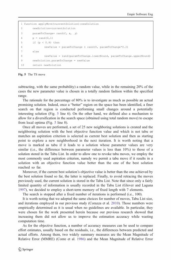
subtracting, with the same probability) a random value, while in the remaining 20% of thecases the new parameter value is chosen in a totally random fashion within the specifiedrange.
The rationale for the percentage of 80% is to investigate as much as possible an actualpromising solution. Indeed, once a “better” region on the space has been identified, a finersearch on that region is conducted performing small changes around a potentiallyinteresting solution (Fig. 5 line 6). On the other hand, we defined also a mechanism toallow for a diversification in the search space (obtained using total random move) to escapefrom local optima (Fig. 5 line 8).
Once all moves are performed, a set of 25 new neighboring solutions is created and theneighboring solution with the best objective function value and which is not tabu ormatches an aspiration criterion is selected as current best solution and then as startingpoint to explore a new neighborhood in the next iteration. It is worth noting that amove is marked as tabu if it leads to a solution whose parameter values are verysimilar (i.e., the difference between parameter values is less than 10%) to those of asolution stored in the Tabu List. In order to allow one to revoke tabu moves, we employ themost commonly used aspiration criterion, namely we permit a tabu move if it results in asolution with an objective function value better than the one of the best solutionreached so far.
Moreover, if the current best solution’s objective value is better than the one achieved bythe best solution found so far, the latter is replaced. Finally, to avoid retracing the movespreviously used, the current solution is stored in the Tabu List. Note that since only a fairlylimited quantity of information is usually recorded in the Tabu List (Glover and Laguna1997), we decided to employ a short-term memory of fixed length with 7 elements.
The search is stopped after a fixed number of iterations is performed (i.e., 100).It is worth noting that we adopted the same choices for number of moves, Tabu List size,
and iterations employed in our previous study (Corazza et al. 2010). Those numbers wereempirically determined as it is usual when no guidelines are available. In particular, theywere chosen for the work presented herein because our previous research showed thatincreasing them did not allow us to improve the estimation accuracy while wastingcomputation time.
As for the objective function, a number of accuracy measures can be used to compareeffort estimates, usually based on the residuals, i.e., the differences between predicted andactual efforts. Among them, two widely summary measures are the Mean Magnitude ofRelative Error (MMRE) (Conte et al. 1986) and the Mean Magnitude of Relative Error
Fig. 5 The TS move
Empir Software Eng
relative to the Estimate (MEMRE) (Kitchenham et al. 2001). Let us recall that MMRE isthe Mean of MRE and MEMRE is the Mean of EMRE, where:
MRE ¼ ebej je
ð2Þ
EMRE ¼ ebej jbe ð3Þ
where e represents actual effort and ê estimated effort. We can observe that EMRE has thesame form of MRE, but the denominator is the estimate, giving thus a stronger penalty tounder-estimates. In (Corazza et al. 2009, 2010, 2011) we employed as objective function,the mean of them:
Objective Function ¼ MMREþMEMREð Þ=2 ð4ÞThe rationale was that, since MRE is more sensitive to overestimates and EMRE to
underestimates, an objective function minimizing them should find better solutions. Sincethe present paper provides a further assessment of the technique proposed in (Corazza et al.2010), we exploited the same objective function.
It is worth noting that the solution we are proposing attempts to capture the necessarydomain knowledge by using performance indicators as the objective function. On the otherhand, it requires a meta-heuristics as robust as possible with respect to the target functioncharacteristics, which are completely unexplored. We think that the TS strategy has thesecharacteristics because of its capability to adapt to the input function both by concentratingsearch efforts on promising areas and keeping away from already visited regions by means ofthe Tabu List.
Finally, in order to cope with the non-deterministic nature of TS, we performed 10 executionsof SVR+TS and, among the obtained configurations, we retained as final the onewhich providedobjective value closest to the mean of the objective values obtained in the 10 executions.
3 Empirical Study Design
In this section, we present the design of the empirical study carried out to assess theeffectiveness of the proposed approach. In particular, we present the employed datasets, thenull hypotheses, the adopted validation method, and evaluation criteria. The results of theempirical analysis are discussed in Section 4.
3.1 Datasets
To carry out the empirical evaluation of the proposed technique we employed a total of 21industry software project datasets selected both from the PROMISE repository (PROMISE2011) and the Tukutuku database (Mendes et al. 2005a). PROMISE contains publiclyavailable single and cross-company datasets, while the Tukutuku database contains dataabout Web projects (i.e., Web hypermedia systems and Web applications) developed indifferent companies and gathered by the Tukutuku project, which aimed to develop Webcost estimation models and to benchmark productivity across and within Web Companies.
Concerning the PROMISE repository, it is worth noting that we did not employ all thedatasets that it contains, since we were interested only on the ones that can be employed for
Empir Software Eng
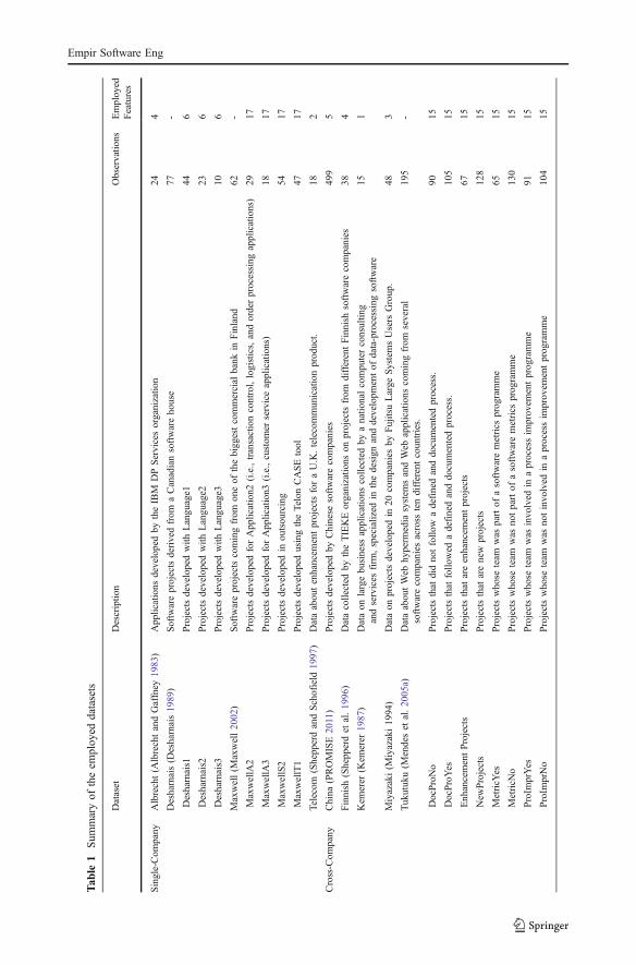
early effort estimation (i.e., datasets containing information that would be available at theearly stages of a software development process), which is the managerial goal of ourinvestigation. To this end, we avoided the use of datasets like NASA and COCOMOcontaining as size measures only features available once a project is completed, such as theLines of Code (LOCs). Moreover, we pruned the remaining datasets from this kind offeatures, since their use could bias the results (Shepperd and Schofield 1997). As for thecategorical variables contained in some datasets, we used them as done in (Kocaguneli et al.2010; Shepperd and Schofield 1997) to obtain different more homogenous splits from theoriginal datasets or we excluded them from our analysis in case splitting was not possible(e.g., the resulting sub datasets were too small). As an example, we used the categoricalvariable “Languages” in the Desharnais dataset to split the original data into three differentdatasets corresponding to Languages 1, 2, and 3, respectively. After applying the abovecriteria, 13 PROMISE datasets were kept for our empirical analysis, namely Albrecht,China, Desharnais1, Desharnais2, Desharnais3, Finnish, Kemerer, MaxwellA2, MaxwellA3,MaxwellS2, MaxwellT1, Miyazaki, and Telecom. We applied the same procedure on theTukutuku database obtaining 8 splits since all the categorical variables (i.e., TypeProj, DocPro,ProImpr, and Metrics) were binary.
Table 1 summarizes the main characteristics of the considered datasets while furtherdetails together with the descriptive statistics of the involved features are provided inAppendix A. They represent an interesting sample of software projects, since they containdata about projects that are Web-based (i.e. the ones from Tukututku) and not Web-based (i.e.,the ones from PROMISE) and include datasets that were collected from a single softwarecompany or several companies.Moreover, all the datasets contain data about industrial projects,representing a diversity of application domains and projects’ characteristics. In particular, theyall differ in relation to:
– geographical locations: software projects coming from Canada, China, Finland, Japan,New Zealand, Italy, United States, etc.;
– number of involved companies;– observation number: from 10 to 499 observations;– number and type of features: from 1 to 27 features, including a variety of features
describing the software and Web projects, such as number of entities in the data model,number of basic, logical transactions, number of developers involved in the project andtheir experience, number of Web page or image;
– technical characteristics: software projects developed in different programminglanguages and for different application domains, ranging from telecommunications tocommercial information systems.
Nevertheless, note that none of these datasets are random samples of software and Webprojects. Therefore the information provided in Appendix A can be useful for readers toassess whether the results we gathered can scale up to their own contexts.
In order to avoid that large differences in the ranges of the features’ values can have theunwanted effect of giving greater importance to some characteristics than to others, a datapreprocessing step should be applied when using SVR (Chang and Lin 2001; Smola andSchölkopf 2004). In our previous studies (Corazza et al. 2009, 2011), we experimenteddifferent preprocessing strategies, such as normalization and logarithmic. The latter is atypical approach in the field of effort estimation (Briand et al. 2000; Costagliola et al. 2006;Di Martino et al. 2007; Kitchenham and Mendes 2004), since it reduces ranges and at thesame time it limits the linearity issue. It provided the best results in (Corazza et al. 2009,2011), thus, we adopted it in (Corazza et al. 2010) and in the present paper. Moreover, we
Empir Software Eng
Tab
le1
Sum
maryof
theem
ploy
eddatasets
Dataset
Descriptio
nObservatio
nsEmployed
Features
Single-Com
pany
Albrecht(A
lbrechtandGaffney
1983)
Applications
developedby
theIBM
DPServicesorganizatio
n24
4
Desharnais(D
esharnais1989)
Softwareprojectsderivedfrom
aCanadiansoftwarehouse
77-
Desharnais1
Projectsdevelopedwith
Language1
446
Desharnais2
Projectsdevelopedwith
Language2
236
Desharnais3
Projectsdevelopedwith
Language3
106
Maxwell(M
axwell2002)
Softwareprojectscomingfrom
oneof
thebiggestcommercial
bank
inFinland
62-
MaxwellA2
ProjectsdevelopedforApplication2
(i.e.,transactioncontrol,logistics,andorderprocessing
applications)
2917
MaxwellA3
ProjectsdevelopedforApplication3
(i.e.,custom
erserviceapplications)
1817
MaxwellS2
Projectsdevelopedin
outsourcing
5417
MaxwellT1
ProjectsdevelopedusingtheTelon
CASEtool
4717
Telecom
(ShepperdandSchofield
1997
)Dataaboutenhancem
entprojectsforaU.K.telecommunicationproduct.
182
Cross-Com
pany
China
(PROMISE2011)
Projectsdevelopedby
Chinese
softwarecompanies
499
5
Finnish
(Shepperdet
al.1996)
Datacollected
bytheTIEKEorganizatio
nson
projectsfrom
differentFinnish
softwarecompanies
384
Kem
erer
(Kem
erer
1987)
Dataon
largebusiness
applications
collected
byanatio
nalcomputerconsultin
gandservices
firm
,specialized
inthedesign
anddevelopm
entof
data-processingsoftware
151
Miyazaki(M
iyazaki1994)
Dataon
projectsdevelopedin
20companies
byFujitsuLarge
SystemsUsers
Group.
483
Tukutuku(M
endeset
al.2005a)
DataaboutWeb
hyperm
edia
system
sandWeb
applications
comingfrom
several
softwarecompanies
across
tendifferentcountries.
195
-
DocProNo
Projectsthat
didnotfollo
wadefinedanddocumentedprocess.
9015
DocProYes
Projectsthat
follo
wed
adefinedanddocumentedprocess.
105
15
EnhancementProjects
Projectsthat
areenhancem
entprojects
6715
New
Projects
Projectsthat
arenew
projects
128
15
MetricY
esProjectswhose
team
was
partof
asoftwaremetrics
programme
6515
MetricN
oProjectswhose
team
was
notpartof
asoftwaremetrics
programme
130
15
ProIm
prYes
Projectswhose
team
was
involved
inaprocessim
provem
entprogramme
9115
ProIm
prNo
Projectswhose
team
was
notinvolved
inaprocessim
provem
entprogramme
104
15
Empir Software Eng
removed from the employed datasets the observations which have missing values (seeAppendix A).
3.2 Null Hypotheses
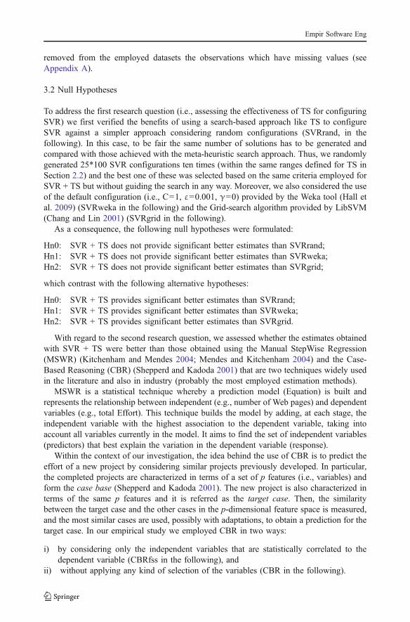
To address the first research question (i.e., assessing the effectiveness of TS for configuringSVR) we first verified the benefits of using a search-based approach like TS to configureSVR against a simpler approach considering random configurations (SVRrand, in thefollowing). In this case, to be fair the same number of solutions has to be generated andcompared with those achieved with the meta-heuristic search approach. Thus, we randomlygenerated 25*100 SVR configurations ten times (within the same ranges defined for TS inSection 2.2) and the best one of these was selected based on the same criteria employed forSVR + TS but without guiding the search in any way. Moreover, we also considered the useof the default configuration (i.e., C=1, ε=0.001, γ=0) provided by the Weka tool (Hall etal. 2009) (SVRweka in the following) and the Grid-search algorithm provided by LibSVM(Chang and Lin 2001) (SVRgrid in the following).
As a consequence, the following null hypotheses were formulated:
Hn0: SVR + TS does not provide significant better estimates than SVRrand;Hn1: SVR + TS does not provide significant better estimates than SVRweka;Hn2: SVR + TS does not provide significant better estimates than SVRgrid;
which contrast with the following alternative hypotheses:
Hn0: SVR + TS provides significant better estimates than SVRrand;Hn1: SVR + TS provides significant better estimates than SVRweka;Hn2: SVR + TS provides significant better estimates than SVRgrid.
With regard to the second research question, we assessed whether the estimates obtainedwith SVR + TS were better than those obtained using the Manual StepWise Regression(MSWR) (Kitchenham and Mendes 2004; Mendes and Kitchenham 2004) and the Case-Based Reasoning (CBR) (Shepperd and Kadoda 2001) that are two techniques widely usedin the literature and also in industry (probably the most employed estimation methods).
MSWR is a statistical technique whereby a prediction model (Equation) is built andrepresents the relationship between independent (e.g., number of Web pages) and dependentvariables (e.g., total Effort). This technique builds the model by adding, at each stage, theindependent variable with the highest association to the dependent variable, taking intoaccount all variables currently in the model. It aims to find the set of independent variables(predictors) that best explain the variation in the dependent variable (response).
Within the context of our investigation, the idea behind the use of CBR is to predict theeffort of a new project by considering similar projects previously developed. In particular,the completed projects are characterized in terms of a set of p features (i.e., variables) andform the case base (Shepperd and Kadoda 2001). The new project is also characterized interms of the same p features and it is referred as the target case. Then, the similaritybetween the target case and the other cases in the p-dimensional feature space is measured,and the most similar cases are used, possibly with adaptations, to obtain a prediction for thetarget case. In our empirical study we employed CBR in two ways:
i) by considering only the independent variables that are statistically correlated to thedependent variable (CBRfss in the following), and
ii) without applying any kind of selection of the variables (CBR in the following).
Empir Software Eng
The key aspects of MSWR and CBR are detailed in Appendix B and C, respectively.In addition, we also assessed whether the estimates obtained with SVR + TS were
significantly better than those obtained using the mean of effort (MeanEffort in thefollowing) and the median of effort (MedianEffort in the following). This was donebecause, as suggested by Mendes and Kitchenham in (2004), if an estimationtechnique does not outperform the results achieved by using MeanEffort andMedianEffort, it cannot be transferred to industry since there would be no value indealing with complex computations of estimation methods to predict development effortcompared to simply using as estimate the mean or the median effort of its own pastprojects.
Thus, we formulated the following null hypotheses:
Hn3: SVR + TS does not provide significant better estimates than MSWR;Hn4: SVR + TS does not provide significant better estimates than CBRfss;Hn5: SVR + TS does not provide significant better estimates than CBR;Hn6: SVR + TS does not provide significant better estimates than MeanEffort;Hn7: SVR + TS does not provide significant better estimates than MedianEffort;
which contrast with the following alternative hypotheses:
Ha3: SVR + TS provides significant better estimates than MSWR;Ha4: SVR + TS provides significantly better estimations than CBRfss;Ha5: SVR + TS provides significantly better estimations than CBR;Ha6: SVR + TS provides significantly better estimations than Mean Effort;Ha7: SVR + TS provides significantly better estimations than Median Effort.
3.3 Validation Method
To assess the effectiveness of the effort predictions obtained using the techniquesemployed herein we exploited a multiple-fold cross validation, partitioning eachoriginal dataset into training sets, for model building, and test sets, for modelevaluation. This is done to avoid optimistic predictions (Briand and Wieczorek 2002).Indeed, cross validation is widely used in the literature to validate effort estimationmodels when dealing with medium/small datasets (e.g., Briand et al. 2000). Whenapplying the multiple-fold cross validation, we decided to use the leave-one-out crossvalidation on the datasets that have less than 60 observations (i.e., Albrecht, Desharnais1,Desharnais2, Desharnais3, Finnish, Kemerer, Miyazaki, and Telecom). In those cases theoriginal datasets of N observations were divided into N different subsets of training andvalidation sets, where each validation set had one project. On the other hand, we decidedto partition the datasets having more than 60 observations (i.e., China and the 8 splitsobtained from the Tukutuku database) into k=10 randomly test sets, and then for each testset to consider the remaining observations as training set to build the estimation model.This choice was made trying to find a trade-off between computational costs andeffectiveness of the validation. The 10 folds for the China datasets are given in Appendix E(Table 10).2
2 We cannot report the 10 folds used for the Tukutuku datasets since the information included in theTukutuku database are not public available, for confidence reasons.
Empir Software Eng
3.4 Evaluation Criteria
Several accuracy measures have been proposed in the literature to assess and comparethe estimates achieved with effort estimation methods (Conte et al. 1986; Kitchenhamet al. 2001), e.g., Mean of MRE, Median of MRE; Mean of EMRE, Median of EMRE,and Pred(25) (i.e., Prediction at level 25%). Considering that all the above measures arebased on the absolute residuals (i.e., the absolute values of differences between predictedand actual efforts) in our empirical analysis we decided to compare the employedestimation techniques in terms of the Median of Absolute Residuals (MdAR), which is acumulative measure widely employed as the Mean of Absolute Residuals (MAR). Wechose to employ MdAR since it is less sensitive to extreme values with respect to MAR(Mendes et al. 2003b). The use of a single summary measure was motivated by the aim toimprove the readability of the discussion on the comparison of the analyzed effortestimation methods (that is not confused by the fact that some measures have to beminimized and other maximized). Moreover, to make the comparison more reliable weused, behind this summary measure, also a statistical test. Indeed, to verify if thedifferences observed using the above measure were legitimate or due to chance, wechecked if the absolute residuals obtained with the application of the various estimationtechniques come from the same population. If they do, it means that there are nosignificant differences between the data values being compared. We accomplished thestatistical significance test using a nonparametric statistical significance test (Kitchenhamet al. 2001), namely Wilcoxon Signed Rank test, with α=0.05. We decided to use theWilcoxon test since it is resilient to strong departures from the t-test assumptions(Conover 1998).
4 Results and Discussion
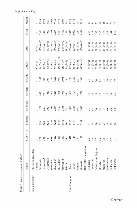
Table 2 reports the Median of the Absolute Residuals (MdAR) obtained with eachtechnique for all the employed datasets. Let us recall that the results of TS + SVR reportedherein were obtained applying on test set the final configuration provided by TS, namelythe one having objective value closest to the mean of the objective values obtained in the 10executions performed on training set. An assessment of the variation of the objective valuescan be found in Appendix D.
Notice that for CBR we used 1, 2, and 3 analogies and due to space constraints, only thebest results are reported herein. The number of analogies used to obtain each of these bestresults is specified in Table 2. The details about the application of MSWR and CBR arereported in Appendix B and C, respectively.
In order to provide better readability, all the best results (i.e., the minimum MdARvalues) obtained for each dataset across the employed techniques are reported in bold (seeTable 2).
Table 2 shows that SVR + TS provided the best MdAR values for all the datasets, exceptfor NewProjects, where CBR provided a slightly better result.
To quantify how much SVR + TS provided better results than the other employedtechniques, for each dataset we calculated the ratio BestSVR/SVR + TS (AvgSVR/SVR + TS, and WorstSVR/SVR + TS, respectively) between the best (the mean, andthe worst, respectively) MdAR provided by the other SVR based approaches with theMdAR of SVR + TS. Similarly, we also provided the same ratios (named BestBench/SVR + TS, AvgBench/SVR + TS, and WorstBench/SVR + TS) with respect to the
Empir Software Eng
Tab
le2
Accuracyin
term
sof
MdA
R
Dataset
SVR+TS
SVRrand
SVRweka
SVRgrid
MSWR
CBRfss
CBR
Mean
Median
Single-Com
pany
PROMISErepository
Albrecht
14
38
45(k=2)
5(k=2)
147
Desharnais1
270
826
1268
803
1142
1457
(k=3)
1738
(k=2)
2316
1589
Desharnais2
490
668
665
2283
1078
1479
(k=3)
1015
(k=3)
3089
1579
Desharnais3
4852
230
210
1330
357
6(k=3)
483(k=3)
1007
812
MaxwellA2
663
1752
2533
1993
2159
4250
(k=1)
3221
(k=2)
5598
4166
MaxwellA3
1394
2697
4515
2449
3084
3639
(k=1)
2236
(k=3)
6005
5598
MaxwellS2
1489
1747
2193
1926
1978
1622
5(k=2)
2552
(k=3)
5473
3473
MaxwellT1
1207
1852
2488
1981
3005
2857
(k=4)
2906
(k=3)
4462
3196
Telecom
2080
7480
5941
(k=2)
41(k=2)
156
168
Cross-Com
pany
China
1032
1335
1090
1082
1138
1326
(k=3)
1326
(k=3)
2833
1329
Finnish
1145
1776
2318
3194
2602
4170
(k=3)
4919
(k=3)
5909
4774
Kem
erer
1461
6665
5256
(k=3)
56(k=3)
125
74
Miyazaki
1175
2197
2483
1739
1936
1976
(k=3)
1976
(k=2)
8338
2832
TUKUTUKU
repository
DocProNo
2641
3343
3864
(k=2)
40(k=2)
287
61
DocProYes
3354
6356
6364
(k=2)
65(k=2)
533
81
Enh
ancementProjects
1724
2418
2450
(k=3)
27(k=3)
192
25
MetricN
o36
5753
5765
60(k=2)
50(k=2)
532
90
MetricY
es12
2415
1514
21(k=1)
24(k=2)
189
164
New
Projects
4749
6057
5657
(k=3)
43(k=3)
548
87
ProIm
prYes
2729
4836
3934
(k=3)
28(k=3)
164
53
ProIm
prNo
4152
5256
4956
(k=3)
54(k=1)
646
84
Empir Software Eng
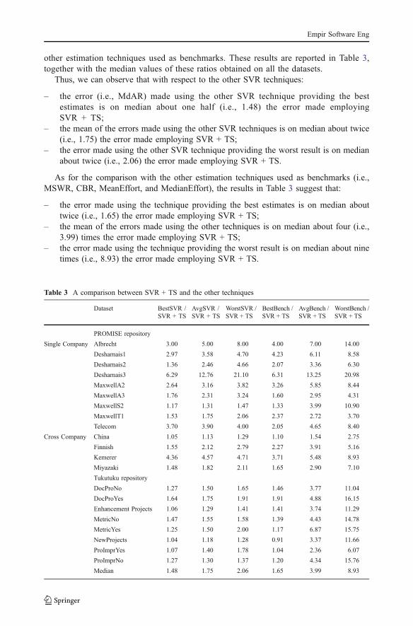
other estimation techniques used as benchmarks. These results are reported in Table 3,together with the median values of these ratios obtained on all the datasets.
Thus, we can observe that with respect to the other SVR techniques:
– the error (i.e., MdAR) made using the other SVR technique providing the bestestimates is on median about one half (i.e., 1.48) the error made employingSVR + TS;
– the mean of the errors made using the other SVR techniques is on median about twice(i.e., 1.75) the error made employing SVR + TS;
– the error made using the other SVR technique providing the worst result is on medianabout twice (i.e., 2.06) the error made employing SVR + TS.
As for the comparison with the other estimation techniques used as benchmarks (i.e.,MSWR, CBR, MeanEffort, and MedianEffort), the results in Table 3 suggest that:
– the error made using the technique providing the best estimates is on median abouttwice (i.e., 1.65) the error made employing SVR + TS;
– the mean of the errors made using the other techniques is on median about four (i.e.,3.99) times the error made employing SVR + TS;
– the error made using the technique providing the worst result is on median about ninetimes (i.e., 8.93) the error made employing SVR + TS.
Table 3 A comparison between SVR + TS and the other techniques
Dataset BestSVR /SVR + TS
AvgSVR /SVR + TS
WorstSVR /SVR + TS
BestBench /SVR + TS
AvgBench /SVR + TS
WorstBench /SVR + TS
PROMISE repository
Single Company Albrecht 3.00 5.00 8.00 4.00 7.00 14.00
Desharnais1 2.97 3.58 4.70 4.23 6.11 8.58
Desharnais2 1.36 2.46 4.66 2.07 3.36 6.30
Desharnais3 6.29 12.76 21.10 6.31 13.25 20.98
MaxwellA2 2.64 3.16 3.82 3.26 5.85 8.44
MaxwellA3 1.76 2.31 3.24 1.60 2.95 4.31
MaxwellS2 1.17 1.31 1.47 1.33 3.99 10.90
MaxwellT1 1.53 1.75 2.06 2.37 2.72 3.70
Telecom 3.70 3.90 4.00 2.05 4.65 8.40
Cross Company China 1.05 1.13 1.29 1.10 1.54 2.75
Finnish 1.55 2.12 2.79 2.27 3.91 5.16
Kemerer 4.36 4.57 4.71 3.71 5.48 8.93
Miyazaki 1.48 1.82 2.11 1.65 2.90 7.10
Tukutuku repository
DocProNo 1.27 1.50 1.65 1.46 3.77 11.04
DocProYes 1.64 1.75 1.91 1.91 4.88 16.15
Enhancement Projects 1.06 1.29 1.41 1.41 3.74 11.29
MetricNo 1.47 1.55 1.58 1.39 4.43 14.78
MetricYes 1.25 1.50 2.00 1.17 6.87 15.75
NewProjects 1.04 1.18 1.28 0.91 3.37 11.66
ProImprYes 1.07 1.40 1.78 1.04 2.36 6.07
ProImprNo 1.27 1.30 1.37 1.20 4.34 15.76
Median 1.48 1.75 2.06 1.65 3.99 8.93
Empir Software Eng
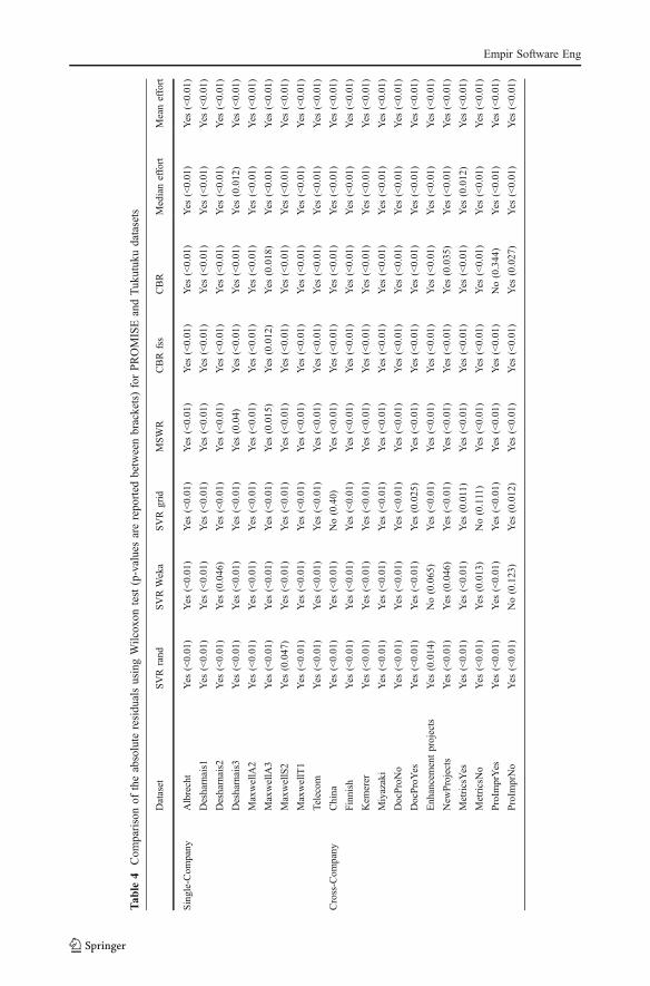
In order to verify whether the differences observed using MdAR values were legitimateor due to chance, we employed the Wilcoxon test (α=0.05) to assess if the absoluteresiduals from all the techniques used came from the same population. The results arereported in Table 4 where “Yes” in a cell means that SVR + TS is significantly superior tothe technique indicated on the column (i.e., it means that the absolute residuals achievedwith SVR + TS are significantly less than the ones obtained with the technique indicated onthe column).
These results allowed us to state that the predictions obtained with SVR + TS weresignificantly superior than those obtained with SVRrand, SVRweka, SVRgrid, MSWR,CBR (with and without feature selection), MedianEffort, and MeanEffort for all PROMISEand Tukutuku datasets, except for a few cases (i.e., the China, EnhancementProjects,MetricNo, ProImprYes, and ProImprNo datasets with respect to SVRgrid, SVRweka,SVRgrid, CBR, and SVRweka approaches, respectively) where no significant differencewas found.
According to these results we can reject all the null hypotheses presented in Section 4(with a confidence of 95%), highlighting that SVR + TS provided significant betterestimates than:
– SVRrand for all the datasets;– SVRweka for 19 out of 21 datasets;– SVRgrid for 19 out of 21 datasets;– MSWR for all the datasets;– CBR for 20 out of 21 datasets;– CBRss for all the datasets;– Mean Effort for all the datasets;– Median Effort for all the datasets.
Thus, we conclude that we can positively answer our research questions, i.e., TabuSearch was able to effectively set Support Vector Regression parameters and the effortpredictions obtained by using the combination of Tabu Search and Support VectorRegression were significantly superior to the ones obtained by other techniques.
Note that these results confirm and extend those previously obtained and detailed in(Corazza et al. 2010), thus supporting the usefulness of TS for configuring SVR. Indeed,TS has allowed us to improve the accuracy of the obtained estimates with respect to the useof random configurations, the use of a default configuration, and the use of the Grid-searchalgorithm for parameter selection provided by LibSVM. Moreover, we want to stress thatthe analysis showed that SVR outperformed the two techniques that are to date the mostwidely and successfully employed prediction techniques in Software Engineering (e.g.,Briand et al. 2000; Briand and Wieczorek 2002; Costagliola et al. 2006; Kitchenham andMendes 2004; Mendes et al. 2008; Mendes and Kitchenham 2004; Shepperd and Kadoda2001), namely MSWR and CBR.
In addition, note that SVR + TS outperformed all the other techniques both for single- andcross- company datasets and for both Web-based and not Web-based applications datasets.
5 Validity Assessment
There are several factors that can bias the validity of empirical studies. Here we considerthree types of validity threats: Construct validity, related to the agreement between atheoretical concept and a specific measuring device or procedure; Conclusion validity,
Empir Software Eng
Tab
le4
Com
parisonof
theabsolute
residu
alsusingWilcox
ontest(p-valuesarerepo
rted
betweenbrackets)forPROMISEandTuk
utukudatasets
Dataset
SVR
rand
SVRWeka
SVRgrid
MSWR
CBR
fss
CBR
Medianeffort
Meaneffort
Single-Com
pany
Albrecht
Yes
(<0.01)
Yes
(<0.01)
Yes
(<0.01)
Yes
(<0.01)
Yes
(<0.01)
Yes
(<0.01)
Yes
(<0.01)
Yes
(<0.01)
Desharnais1
Yes
(<0.01)
Yes
(<0.01)
Yes
(<0.01)
Yes
(<0.01)
Yes
(<0.01)
Yes
(<0.01)
Yes
(<0.01)
Yes
(<0.01)
Desharnais2
Yes
(<0.01)
Yes
(0.046)
Yes
(<0.01)
Yes
(<0.01)
Yes
(<0.01)
Yes
(<0.01)
Yes
(<0.01)
Yes
(<0.01)
Desharnais3
Yes
(<0.01)
Yes
(<0.01)
Yes
(<0.01)
Yes
(0.04)
Yes
(<0.01)
Yes
(<0.01)
Yes
(0.012)
Yes
(<0.01)
MaxwellA2
Yes
(<0.01)
Yes
(<0.01)
Yes
(<0.01)
Yes
(<0.01)
Yes
(<0.01)
Yes
(<0.01)
Yes
(<0.01)
Yes
(<0.01)
MaxwellA3
Yes
(<0.01)
Yes
(<0.01)
Yes
(<0.01)
Yes
(0.015)
Yes
(0.012)
Yes
(0.018)
Yes
(<0.01)
Yes
(<0.01)
MaxwellS2
Yes
(0.047)
Yes
(<0.01)
Yes
(<0.01)
Yes
(<0.01)
Yes
(<0.01)
Yes
(<0.01)
Yes
(<0.01)
Yes
(<0.01)
MaxwellT1
Yes
(<0.01)
Yes
(<0.01)
Yes
(<0.01)
Yes
(<0.01)
Yes
(<0.01)
Yes
(<0.01)
Yes
(<0.01)
Yes
(<0.01)
Telecom
Yes
(<0.01)
Yes
(<0.01)
Yes
(<0.01)
Yes
(<0.01)
Yes
(<0.01)
Yes
(<0.01)
Yes
(<0.01)
Yes
(<0.01)
Cross-Com
pany
China
Yes
(<0.01)
Yes
(<0.01)
No(0.40)
Yes
(<0.01)
Yes
(<0.01)
Yes
(<0.01)
Yes
(<0.01)
Yes
(<0.01)
Finnish
Yes
(<0.01)
Yes
(<0.01)
Yes
(<0.01)
Yes
(<0.01)
Yes
(<0.01)
Yes
(<0.01)
Yes
(<0.01)
Yes
(<0.01)
Kem
erer
Yes
(<0.01)
Yes
(<0.01)
Yes
(<0.01)
Yes
(<0.01)
Yes
(<0.01)
Yes
(<0.01)
Yes
(<0.01)
Yes
(<0.01)
Miyazaki
Yes
(<0.01)
Yes
(<0.01)
Yes
(<0.01)
Yes
(<0.01)
Yes
(<0.01)
Yes
(<0.01)
Yes
(<0.01)
Yes
(<0.01)
DocProNo
Yes
(<0.01)
Yes
(<0.01)
Yes
(<0.01)
Yes
(<0.01)
Yes
(<0.01)
Yes
(<0.01)
Yes
(<0.01)
Yes
(<0.01)
DocProYes
Yes
(<0.01)
Yes
(<0.01)
Yes
(0.025)
Yes
(<0.01)
Yes
(<0.01)
Yes
(<0.01)
Yes
(<0.01)
Yes
(<0.01)
Enhancementprojects
Yes
(0.014)
No(0.065)
Yes
(<0.01)
Yes
(<0.01)
Yes
(<0.01)
Yes
(<0.01)
Yes
(<0.01)
Yes
(<0.01)
New
Projects
Yes
(<0.01)
Yes
(0.046)
Yes
(<0.01)
Yes
(<0.01)
Yes
(<0.01)
Yes
(0.035)
Yes
(<0.01)
Yes
(<0.01)
MetricsYes
Yes
(<0.01)
Yes
(<0.01)
Yes
(0.011)
Yes
(<0.01)
Yes
(<0.01)
Yes
(<0.01)
Yes
(0.012)
Yes
(<0.01)
MetricsNo
Yes
(<0.01)
Yes
(0.013)
No(0.111)
Yes
(<0.01)
Yes
(<0.01)
Yes
(<0.01)
Yes
(<0.01)
Yes
(<0.01)
ProIm
prYes
Yes
(<0.01)
Yes
(<0.01)
Yes
(<0.01)
Yes
(<0.01)
Yes
(<0.01)
No(0.344)
Yes
(<0.01)
Yes
(<0.01)
ProIm
prNo
Yes
(<0.01)
No(0.123)
Yes
(0.012)
Yes
(<0.01)
Yes
(<0.01)
Yes
(0.027)
Yes
(<0.01)
Yes
(<0.01)
Empir Software Eng
related to the ability to draw statistically correct conclusions; External validity, related to theability to generalise the achieved results. As highlighted by Kitchenham et al. (1995), tosatisfy construct validity a study has “to establish correct operational measures for theconcepts being studied”. Thus, the choice of the features and how to collect them representsthe crucial aspects. We mitigated such a threat by evaluating the employed estimationmethods on publicly available datasets from the PROMISE repository. These datasets havebeen previously used in many other empirical studies carried out to evaluate effortestimation methods (see PROMISE web site).
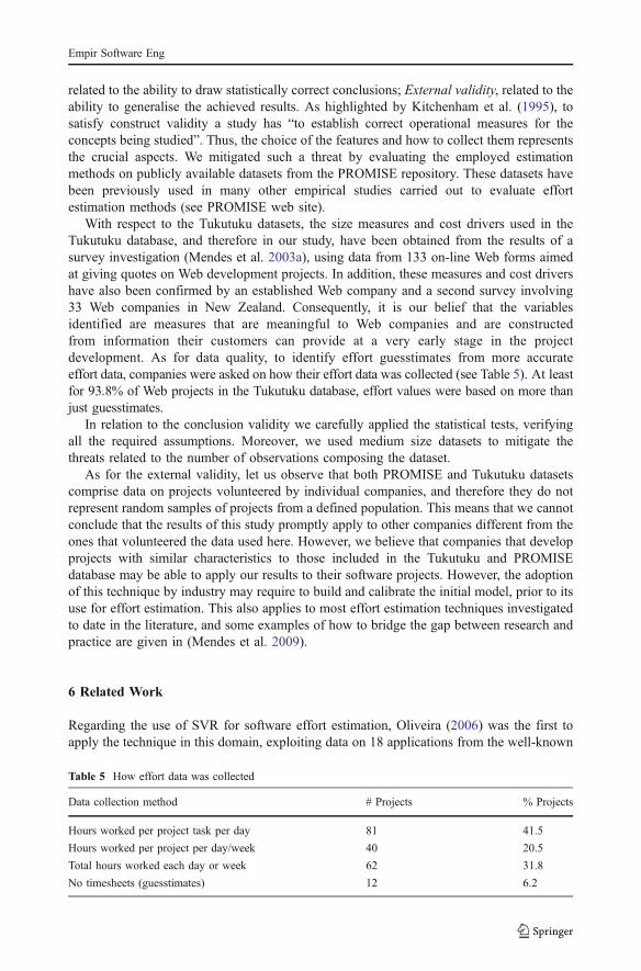
With respect to the Tukutuku datasets, the size measures and cost drivers used in theTukutuku database, and therefore in our study, have been obtained from the results of asurvey investigation (Mendes et al. 2003a), using data from 133 on-line Web forms aimedat giving quotes on Web development projects. In addition, these measures and cost drivershave also been confirmed by an established Web company and a second survey involving33 Web companies in New Zealand. Consequently, it is our belief that the variablesidentified are measures that are meaningful to Web companies and are constructedfrom information their customers can provide at a very early stage in the projectdevelopment. As for data quality, to identify effort guesstimates from more accurateeffort data, companies were asked on how their effort data was collected (see Table 5). At leastfor 93.8% of Web projects in the Tukutuku database, effort values were based on more thanjust guesstimates.
In relation to the conclusion validity we carefully applied the statistical tests, verifyingall the required assumptions. Moreover, we used medium size datasets to mitigate thethreats related to the number of observations composing the dataset.
As for the external validity, let us observe that both PROMISE and Tukutuku datasetscomprise data on projects volunteered by individual companies, and therefore they do notrepresent random samples of projects from a defined population. This means that we cannotconclude that the results of this study promptly apply to other companies different from theones that volunteered the data used here. However, we believe that companies that developprojects with similar characteristics to those included in the Tukutuku and PROMISEdatabase may be able to apply our results to their software projects. However, the adoptionof this technique by industry may require to build and calibrate the initial model, prior to itsuse for effort estimation. This also applies to most effort estimation techniques investigatedto date in the literature, and some examples of how to bridge the gap between research andpractice are given in (Mendes et al. 2009).
6 Related Work
Regarding the use of SVR for software effort estimation, Oliveira (2006) was the first toapply the technique in this domain, exploiting data on 18 applications from the well-known
Table 5 How effort data was collected
Data collection method # Projects % Projects
Hours worked per project task per day 81 41.5
Hours worked per project per day/week 40 20.5
Total hours worked each day or week 62 31.8
No timesheets (guesstimates) 12 6.2
Empir Software Eng
NASA software project dataset (Bailey and Basili 1981). The author tested the linear andthe RBF kernels, trying for each of them three settings for the SVR’s parameters. Theevaluation, conducted using a leave-one-out cross-validation, and expressed in terms of theindicators MMRE and Pred(25), highlighted that SVR significantly outperformed bothLinear Regression and Radial Basis Function Networks (RBFNs). In a subsequent study,Braga et al. (2007) proposed a machine learning-based method able to provide an effortestimate and a corresponding confidence interval. To assess the defined method, theyperformed a case study using the Desharnais (Desharnais 1989) and NASA (Bailey andBasili 1981) datasets. The results of this empirical analysis showed that the proposedmethod was characterized by better performance with respect to the previous study. It isworth noting that we cannot perform a punctual comparison of our results with thosepresented in that work, since authors used a hold-out validation on the Desharnias dataset,obtained by randomly selecting 18 projects as training set, but did not report whose projectsthey exploited. As for NASA, as said in section 3.1 we excluded it from our analysis sinceit contains only LOC as size measure.
We also previously employed SVR (Corazza et al. 2009, 2011) and SVR + TS (Corazzaet al. 2010), as detailed in Sections 1 and 2.
As for the use of meta-heuristics to explore the parameter setting with the aim toimprove effort predictions, this is a quite new research. Some research has been conductedto employ Genetic Algorithms (GA) to improve the estimation performance of existingestimation techniques. To the best of our knowledge, the first attempt to combineevolutionary approaches with an existing effort estimation technique was made by Shukla(2000) applying GA to Neural Networks (NN) predictor (namely, neuro-genetic approach,GANN) to improve its estimation capability. Results were significantly better than othertechniques, such as a modified version of the Regression Trees.
Li et al. (2009) proposed a combination of an evolutionary approach with CBR, aimingat exploiting GA to simultaneously optimize the selection of the feature weights andprojects. The performed case study employed a hold-out validation on the Desharnais,Albrecht, and two artificial datasets. The results showed that the use of GA can providesignificantly better estimations. Also in this case, we cannot compare our results with thosepresented in that paper since the datasets have been handled differently.
More recently, Chiu and Huang (2007) applied GA to many different analogy-basedapproaches using two datasets not included in the PROMISE repository. The results showed animprovement of 38% in terms of MMRE, when using GA to explore an adjustment function.
About Tabu Search, to the best of our knowledge, only two case studies were performedto assess its use for estimating software development effort. In particular, Ferrucci et al.applied TS on Desharnais (Ferrucci et al. 2009) and Tukutuku datasets (Ferrucci et al.2010), obtaining interesting results, motivating further investigation on the use of search-based methods in this field.
7 Conclusions and Future Work
In this paper, we have assessed whether Support Vector Regression configured by using theproposed Tabu Search approach can be effective to estimate software development effort.We extended a previous empirical study (Corazza et al. 2010) where we applied SVR + TSto two splits randomly obtained from 195 applications of the Tukutuku database andapplying a hold-out cross validation. The results obtained were promising and encouragedus to further verify the effectiveness of SVR + TS. In particular, in this paper we have
Empir Software Eng
presented the results achieved by applying SVR + TS to other 13 datasets obtained from thePROMISE repository and considering further 8 datasets obtained by splitting the Tukutukudatabase according to the values of 4 categorical variables included in it. Thus, a total of 21datasets (both single- and cross- company datasets related to both Web-based and not Web-based applications) were employed to perform a 10-fold or a leave-one-out validationdepending on the size of the datasets.
Regarding the choices of SVR kernels and pre-processing strategy, we have employedthe RBF kernel and a logarithmic transformation of the variables since they provided thebest results in (Corazza et al. 2010).
The results of the empirical analysis have confirmed and extended those reported in(Corazza et al. 2010), highlighting the goodness of TS for configuring SVR. Indeed, SVR +TS provided significant better estimates than SVR configured with simpler approaches,such as random configuration, default configuration provided by the Weka tool, and theGrid-search algorithm provided by LibSVM. Moreover, SVR + TS allowed us to obtainsignificantly better effort estimates than the ones obtained using MSWR and CBR, twotechniques widely employed both in academic and industrial contexts.
Many studies have been reported in the literature that show the ability of SVR to constructaccurate predictive models in different contexts (Cherkassky and Ma 2004). Nevertheless,those studies are usually based on the opinion of experts that select SVR parameter values onthe basis of their knowledge of both the approach and the application domain (Cherkasskyand Ma 2004). Of course the reliance upon experts severely bounds the practical applicabilityof this approach in the software industries. The approach investigated in the present paperdoes not only address the problem to find a suitable SVR setting for effort estimation but italso allows practitioners of software industries to effectively use it without requiring to be anexpert in the field of those techniques. Indeed, although the models constructed using thedatasets employed in the present paper cannot be immediately adopted in other softwarecompanies, thanks to the use of the proposed approach project managers can automaticallybuild their own effort estimation models starting from their historical data.
These observations together with the results presented in this paper suggest SVR + TSamong the techniques that are suitable for software development effort estimation inindustrial world.
Several interesting investigations can be planned as future work. First of all, otherobjective functions could be exploited in the definition of TS and their influence on thefinal results could be analyzed. These functions could be based on other evaluation criteria(e.g., Pred(25)) used to compare effort estimation models or based on measures optimizedby other estimation techniques (e.g., SSR optimized by MSWR). Other aspects of TS couldalso be investigated, such as the use of a heuristics to choose the initial solution and thencompare the results with respect to the random initialization employed in the present paper.
Finally, the good results herein reported concerning the ability of TS to configure SVRencourage us to apply a similar approach to other estimation techniques, such as CBR (forexample to select feature and/or other aspects, such as the number of analogies).
Acknowledgments Authors would like to thank the anonymous reviewers for their valuable comments andsuggestions and all companies that volunteered data to the Tukutuku database and to the PROMISErepository. The research has been carried out also exploiting the computer systems funded by University ofSalerno’s Finanziamento Medie e Grandi Attrezzature (2005).
Open Access This article is distributed under the terms of the Creative Commons AttributionNoncommercial License which permits any noncommercial use, distribution, and reproduction in anymedium, provided the original author(s) and source are credited.
Empir Software Eng
Appendix
A. Datasets Descriptions
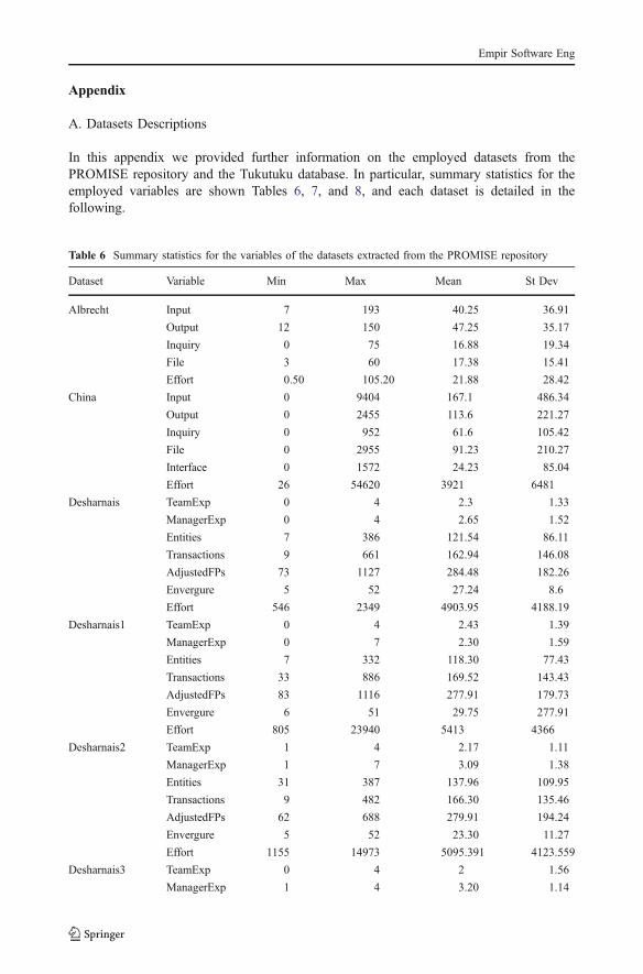
In this appendix we provided further information on the employed datasets from thePROMISE repository and the Tukutuku database. In particular, summary statistics for theemployed variables are shown Tables 6, 7, and 8, and each dataset is detailed in thefollowing.
Table 6 Summary statistics for the variables of the datasets extracted from the PROMISE repository
Dataset Variable Min Max Mean St Dev
Albrecht Input 7 193 40.25 36.91
Output 12 150 47.25 35.17
Inquiry 0 75 16.88 19.34
File 3 60 17.38 15.41
Effort 0.50 105.20 21.88 28.42
China Input 0 9404 167.1 486.34
Output 0 2455 113.6 221.27
Inquiry 0 952 61.6 105.42
File 0 2955 91.23 210.27
Interface 0 1572 24.23 85.04
Effort 26 54620 3921 6481
Desharnais TeamExp 0 4 2.3 1.33
ManagerExp 0 4 2.65 1.52
Entities 7 386 121.54 86.11
Transactions 9 661 162.94 146.08
AdjustedFPs 73 1127 284.48 182.26
Envergure 5 52 27.24 8.6
Effort 546 2349 4903.95 4188.19
Desharnais1 TeamExp 0 4 2.43 1.39
ManagerExp 0 7 2.30 1.59
Entities 7 332 118.30 77.43
Transactions 33 886 169.52 143.43
AdjustedFPs 83 1116 277.91 179.73
Envergure 6 51 29.75 277.91
Effort 805 23940 5413 4366
Desharnais2 TeamExp 1 4 2.17 1.11
ManagerExp 1 7 3.09 1.38
Entities 31 387 137.96 109.95
Transactions 9 482 166.30 135.46
AdjustedFPs 62 688 279.91 194.24
Envergure 5 52 23.30 11.27
Effort 1155 14973 5095.391 4123.559
Desharnais3 TeamExp 0 4 2 1.56
ManagerExp 1 4 3.20 1.14
Empir Software Eng
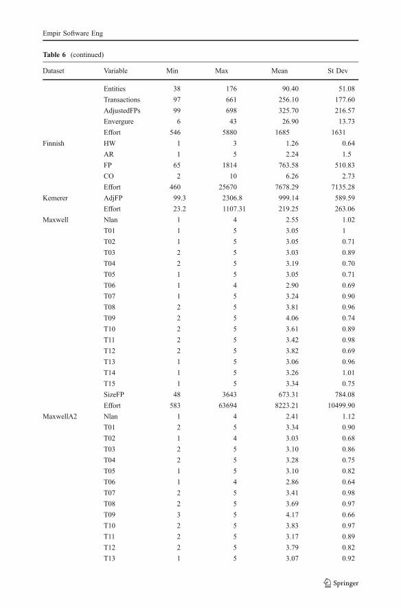
Table 6 (continued)
Dataset Variable Min Max Mean St Dev
Entities 38 176 90.40 51.08
Transactions 97 661 256.10 177.60
AdjustedFPs 99 698 325.70 216.57
Envergure 6 43 26.90 13.73
Effort 546 5880 1685 1631
Finnish HW 1 3 1.26 0.64
AR 1 5 2.24 1.5
FP 65 1814 763.58 510.83
CO 2 10 6.26 2.73
Effort 460 25670 7678.29 7135.28
Kemerer AdjFP 99.3 2306.8 999.14 589.59
Effort 23.2 1107.31 219.25 263.06
Maxwell Nlan 1 4 2.55 1.02
T01 1 5 3.05 1
T02 1 5 3.05 0.71
T03 2 5 3.03 0.89
T04 2 5 3.19 0.70
T05 1 5 3.05 0.71
T06 1 4 2.90 0.69
T07 1 5 3.24 0.90
T08 2 5 3.81 0.96
T09 2 5 4.06 0.74
T10 2 5 3.61 0.89
T11 2 5 3.42 0.98
T12 2 5 3.82 0.69
T13 1 5 3.06 0.96
T14 1 5 3.26 1.01
T15 1 5 3.34 0.75
SizeFP 48 3643 673.31 784.08
Effort 583 63694 8223.21 10499.90
MaxwellA2 Nlan 1 4 2.41 1.12
T01 2 5 3.34 0.90
T02 1 4 3.03 0.68
T03 2 5 3.10 0.86
T04 2 5 3.28 0.75
T05 1 5 3.10 0.82
T06 1 4 2.86 0.64
T07 2 5 3.41 0.98
T08 2 5 3.69 0.97
T09 3 5 4.17 0.66
T10 2 5 3.83 0.97
T11 2 5 3.17 0.89
T12 2 5 3.79 0.82
T13 1 5 3.07 0.92
Empir Software Eng
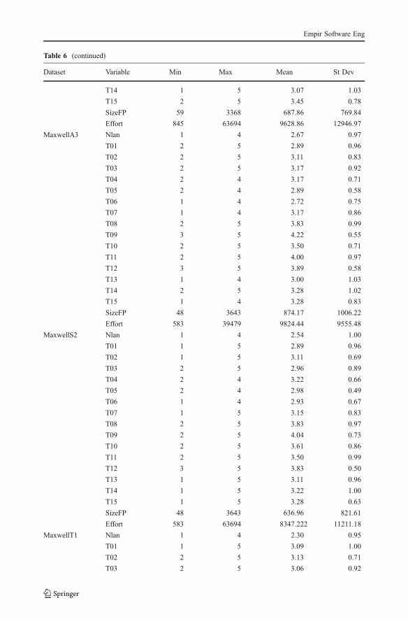
Table 6 (continued)
Dataset Variable Min Max Mean St Dev
T14 1 5 3.07 1.03
T15 2 5 3.45 0.78
SizeFP 59 3368 687.86 769.84
Effort 845 63694 9628.86 12946.97
MaxwellA3 Nlan 1 4 2.67 0.97
T01 2 5 2.89 0.96
T02 2 5 3.11 0.83
T03 2 5 3.17 0.92
T04 2 4 3.17 0.71
T05 2 4 2.89 0.58
T06 1 4 2.72 0.75
T07 1 4 3.17 0.86
T08 2 5 3.83 0.99
T09 3 5 4.22 0.55
T10 2 5 3.50 0.71
T11 2 5 4.00 0.97
T12 3 5 3.89 0.58
T13 1 4 3.00 1.03
T14 2 5 3.28 1.02
T15 1 4 3.28 0.83
SizeFP 48 3643 874.17 1006.22
Effort 583 39479 9824.44 9555.48
MaxwellS2 Nlan 1 4 2.54 1.00
T01 1 5 2.89 0.96
T02 1 5 3.11 0.69
T03 2 5 2.96 0.89
T04 2 4 3.22 0.66
T05 2 4 2.98 0.49
T06 1 4 2.93 0.67
T07 1 5 3.15 0.83
T08 2 5 3.83 0.97
T09 2 5 4.04 0.73
T10 2 5 3.61 0.86
T11 2 5 3.50 0.99
T12 3 5 3.83 0.50
T13 1 5 3.11 0.96
T14 1 5 3.22 1.00
T15 1 5 3.28 0.63
SizeFP 48 3643 636.96 821.61
Effort 583 63694 8347.222 11211.18
MaxwellT1 Nlan 1 4 2.30 0.95
T01 1 5 3.09 1.00
T02 2 5 3.13 0.71
T03 2 5 3.06 0.92
Empir Software Eng
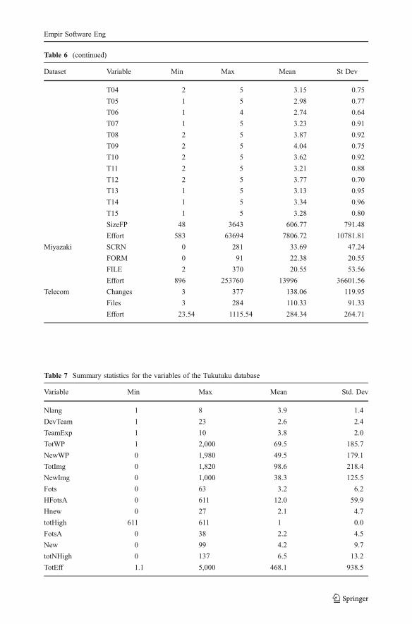
Table 6 (continued)
Dataset Variable Min Max Mean St Dev
T04 2 5 3.15 0.75
T05 1 5 2.98 0.77
T06 1 4 2.74 0.64
T07 1 5 3.23 0.91
T08 2 5 3.87 0.92
T09 2 5 4.04 0.75
T10 2 5 3.62 0.92
T11 2 5 3.21 0.88
T12 2 5 3.77 0.70
T13 1 5 3.13 0.95
T14 1 5 3.34 0.96
T15 1 5 3.28 0.80
SizeFP 48 3643 606.77 791.48
Effort 583 63694 7806.72 10781.81
Miyazaki SCRN 0 281 33.69 47.24
FORM 0 91 22.38 20.55
FILE 2 370 20.55 53.56
Effort 896 253760 13996 36601.56
Telecom Changes 3 377 138.06 119.95
Files 3 284 110.33 91.33
Effort 23.54 1115.54 284.34 264.71
Table 7 Summary statistics for the variables of the Tukutuku database
Variable Min Max Mean Std. Dev
Nlang 1 8 3.9 1.4
DevTeam 1 23 2.6 2.4
TeamExp 1 10 3.8 2.0
TotWP 1 2,000 69.5 185.7
NewWP 0 1,980 49.5 179.1
TotImg 0 1,820 98.6 218.4
NewImg 0 1,000 38.3 125.5
Fots 0 63 3.2 6.2
HFotsA 0 611 12.0 59.9
Hnew 0 27 2.1 4.7
totHigh 611 611 1 0.0
FotsA 0 38 2.2 4.5
New 0 99 4.2 9.7
totNHigh 0 137 6.5 13.2
TotEff 1.1 5,000 468.1 938.5
Empir Software Eng
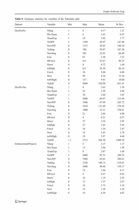
Table 8 Summary statistics for variables of the Tukutuku split
Dataset Variable Min Max Mean St Dev
DocProNo Nlang 1 8 4.17 1.21
DevTeam 1 6 1.63 0.97
TeamExp 1 10 5.02 1.77
TotWP 3 1390 49.07 147.96
NewWP 0 1333 28.03 140.10
TotImg 0 780 59.97 107.38
NewImg 0 583 22.01 66.49
Fots 0 63 3.58 7.53
HFotsA 0 611 25.67 86.35
Hnew 0 8 0.72 1.84
totHigh 0 611 26.39 86.16
FotsA 0 38 3.06 6.04
New 0 99 6.36 13.34
totNHigh 0 137 9.41 18.60
TotEff 4 5000 350.90 851.41
DocProYes Nlang 1 8 3.65 1.59
DevTeam 1 23 3.39 2.88
TeamExp 1 10 2.80 1.65
TotWP 1 2000 86.97 211.94
NewWP 0 1980 67.99 205.72
TotImg 0 1820 131.69 276.92
NewImg 0 1000 52.21 158.61
Fots 0 21 2.86 4.90
HFotsA 0 4 0.21 0.57
Hnew 0 27 3.24 5.95
totHigh 0 27 3.45 5.93
FotsA 0 16 1.54 2.47
New 0 19 2.43 3.78
totNHigh 0 19 3.97 4.04
TotEff 1.1 3712 568.58 1000.30
EnhancementProjects Nlang 1 6 3.15 1.17
DevTeam 1 15 2.46 1.94
TeamExp 1 8 2.87 1.60
TotWP 1 2000 97.51 299.33
NewWP 0 1980 65.03 289.61
TotImg 0 1238 100.73 219.81
NewImg 0 1000 48.46 150.17
Fots 0 19 1.84 4.17
HFotsA 0 4 0.37 0.85
Hnew 0 10 1.19 2.43
totHigh 0 12 1.57 2.67
FotsA 0 16 2.72 3.10
New 0 19 1.58 3.39
totNHigh 0 19 4.30 4.07
Empir Software Eng
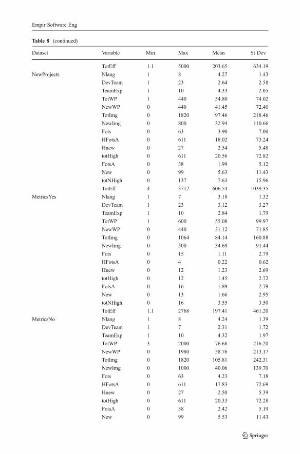
Table 8 (continued)
Dataset Variable Min Max Mean St Dev
TotEff 1.1 5000 203.65 634.19
NewProjects Nlang 1 8 4.27 1.43
DevTeam 1 23 2.64 2.58
TeamExp 1 10 4.33 2.05
TotWP 1 440 54.80 74.02
NewWP 0 440 41.45 72.40
TotImg 0 1820 97.46 218.46
NewImg 0 800 32.94 110.66
Fots 0 63 3.90 7.00
HFotsA 0 611 18.02 73.24
Hnew 0 27 2.54 5.48
totHigh 0 611 20.56 72.82
FotsA 0 38 1.99 5.12
New 0 99 5.63 11.43
totNHigh 0 137 7.63 15.96
TotEff 4 3712 606.54 1039.35
MetricsYes Nlang 1 7 3.18 1.32
DevTeam 1 23 3.12 3.27
TeamExp 1 10 2.84 1.79
TotWP 1 600 55.08 99.97
NewWP 0 440 31.12 71.85
TotImg 0 1064 84.14 160.88
NewImg 0 500 34.69 91.44
Fots 0 15 1.11 2.79
HFotsA 0 4 0.22 0.62
Hnew 0 12 1.23 2.69
totHigh 0 12 1.45 2.72
FotsA 0 16 1.89 2.79
New 0 13 1.66 2.95
totNHigh 0 16 3.55 3.50
TotEff 1.1 2768 197.41 461.20
MetricsNo Nlang 1 8 4.24 1.39
DevTeam 1 7 2.31 1.72
TeamExp 1 10 4.32 1.97
TotWP 3 2000 76.68 216.20
NewWP 0 1980 58.76 213.17
TotImg 0 1820 105.81 242.31
NewImg 0 1000 40.06 139.70
Fots 0 63 4.23 7.18
HFotsA 0 611 17.83 72.69
Hnew 0 27 2.50 5.39
totHigh 0 611 20.33 72.28
FotsA 0 38 2.42 5.19
New 0 99 5.53 11.43
Empir Software Eng
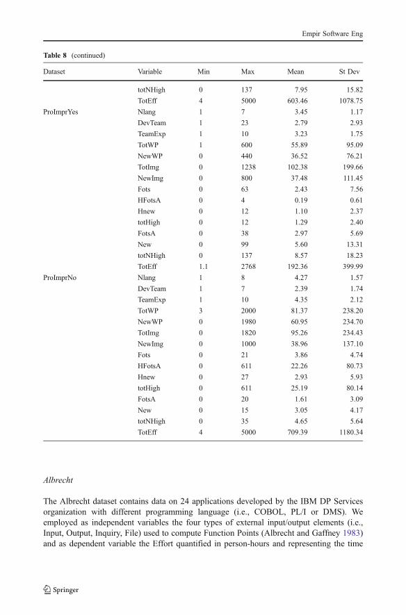
Albrecht
The Albrecht dataset contains data on 24 applications developed by the IBM DP Servicesorganization with different programming language (i.e., COBOL, PL/I or DMS). Weemployed as independent variables the four types of external input/output elements (i.e.,Input, Output, Inquiry, File) used to compute Function Points (Albrecht and Gaffney 1983)and as dependent variable the Effort quantified in person-hours and representing the time
Table 8 (continued)
Dataset Variable Min Max Mean St Dev
totNHigh 0 137 7.95 15.82
TotEff 4 5000 603.46 1078.75
ProImprYes Nlang 1 7 3.45 1.17
DevTeam 1 23 2.79 2.93
TeamExp 1 10 3.23 1.75
TotWP 1 600 55.89 95.09
NewWP 0 440 36.52 76.21
TotImg 0 1238 102.38 199.66
NewImg 0 800 37.48 111.45
Fots 0 63 2.43 7.56
HFotsA 0 4 0.19 0.61
Hnew 0 12 1.10 2.37
totHigh 0 12 1.29 2.40
FotsA 0 38 2.97 5.69
New 0 99 5.60 13.31
totNHigh 0 137 8.57 18.23
TotEff 1.1 2768 192.36 399.99
ProImprNo Nlang 1 8 4.27 1.57
DevTeam 1 7 2.39 1.74
TeamExp 1 10 4.35 2.12
TotWP 3 2000 81.37 238.20
NewWP 0 1980 60.95 234.70
TotImg 0 1820 95.26 234.43
NewImg 0 1000 38.96 137.10
Fots 0 21 3.86 4.74
HFotsA 0 611 22.26 80.73
Hnew 0 27 2.93 5.93
totHigh 0 611 25.19 80.14
FotsA 0 20 1.61 3.09
New 0 15 3.05 4.17
totNHigh 0 35 4.65 5.64
TotEff 4 5000 709.39 1180.34
Empir Software Eng
employed to design, develop, and test each application. We excluded from the analysis thenumber of SLOC.
China
The China dataset contains data on 499 projects developed in China by various softwarecompanies in multiple business domains. We employed as independent variables theexternal input/output elements used to calculate Function Points (i.e., Input, Output,Inquiry, File, Interface) and Effort as dependent variable (PROMISE 2011).
Desharnais
Desharnais (Desharnais 1989) has been widely used to evaluate estimation methods, e.g.,(Burgess and Lefley 2001; Ferrucci et al. 2009; Shepperd and Schofield 1997; Shepperd etal. 1996). It contains data about 81, but we excluded four projects that have some missingvalues, as done in other studies (e.g., Shepperd and Schofield 1997; Shepperd et al. 1996).
As independent variables we employed: TeamExp (i.e., the team experience measured inyears), ManagerExp (i.e., the manager experience measured in years), Entities (i.e., thenumber of the entities in the system data model), Transactions (i.e., the number of basiclogical transactions in the system), AdjustedFPs (i.e., the adjusted Function Points), andEnvergure (i.e., a complex measure derived from other factors defining the environment).We considered as dependent variable the total effort while we excluded the length of thecode. The categorical variable YearEnd was also excluded from the analysis as done inother works (e.g., Kocaguneli et al. 2010; Shepperd and Kadoda 2001) since this not aninformation that could influence the effort prediction of new applications. The othercategorical variable, namely Languages, was used (as done in Kocaguneli et al. 2010;Shepperd and Schofield 1997) to split the original dataset into three different datasetsDesharnais1 (having 44 observations), Desharnais2 (having 23 observations), andDesharnais3 (having 10 observations) corresponding to Languages 1, 2, and 3, respectively.
Finnish
Finnish contains data on 38 projects from different Finnish companies (Shepperd et al.1996). In particular, the dataset consists of a dependent variable, the Effort expressed inperson-hours, and five independent variables. We decided to do not consider the PRODvariable because it represents the productivity expressed in terms of Effort and size (FP).
Kemerer
The Kemerer dataset (Kemerer 1987) contains 15 large business applications, 12 ofwhich were written entirely in Cobol. In particular, for each application the number ofboth adjusted and raw function points is reported (only AdjFP has been exploited in ourstudy). The Effort is the total number of actual hours expended by staff members (i.e., notincluding secretarial labor) on the project through implementation, divided by 152. Weexcluded from our analysis the KSLOC variable which counts the thousands of deliveredsource instructions, the variable Duration, which represents the project durations in
Empir Software Eng
calendar months, and two categorical variables, Software and Hardware, that indicate thesoftware (i.e., Bliss, Cobol, Natural) and the hardware (e.g., IBM 308X, IBM 43XX,DEC Vax) employed in each project, respectively. Note that differently from Desharnaisdataset these categorical variables could not be used to create subsets since the resultingsets were too small.
Maxwell
The Maxwell dataset (Maxwell 2002) contains data of 62 projects in terms of 17 features:Function Points and 16 ordinal variables, i.e., number of different development languagesused (Nlan), customer participation (T01), development environment adequacy (T02), staffavailability (T03), standards used (T04), methods used (T05), tools used (T06), software’slogical complexity (T07), requirements volatility (T08), quality requirements (T09), efficiencyrequirements (T10), installation requirements (T11), staff analysis skills (T12), staffapplication knowledge (T13), staff tool skills (T14), staff team skills (T15). As done for theDesharnais dataset, we used the categorical variables to split the original dataset. In particular,using the three variables, App, Source, and TelonUse (the former indicates the applicationtype, the second indicates in-house or outsourcing development, and the last indicateswhether the Telon CASE tool was employed) we obtained 9 datasets, however only thosedatasets having a number of observations greater than the feature number were used in ourexperimentation. In particular, we employed the set of 29 observations having App equals to2, the set of 18 observations having App equals to 3, the set of 54 observation having Sourceequals to 2, and the set of 47 observations having TelonUse equals to 1. In the following werefer to these datasets as MaxwellA2, MaxwellA3, MaxwellS2, and MaxwellT1, respectively.
Miyazaki
The Miyazaki dataset is composed by projects data collected from 48 systems in 20Japanese companies by Fujitsu Large Systems Users Group (Miyazaki et al. 1994). Weconsidered the independent variables SCRN (i.e., the number of different input or outputscreen formats), and FORM (i.e., the number of different form) as done in (Miyazaki et al.1994). The dependent variable is the Effort defined as the number of person-hours neededfrom system design to system test, including indirect effort such as project management.
Telecom
Telecom includes information on two independent variables, i.e., Changes and Files, andthe dependent variable Effort (Shepperd and Schofield 1997). Changes represents thenumber of changes made as recorded by the configuration management system and Files isthe number of files changed by the particular enhancement project.
Tukutuku
The Tukutuku database (Mendes et al. 2005a) contains Web hypermedia systems and Webapplications. The former are characterized by the authoring of information using nodes(chunks of information), links (relations between nodes), anchors, access structures (for
Empir Software Eng
navigation) and its delivery over the Web. Conversely, the latter represent softwareapplications that depend on the Web or use the Web’s infrastructure for execution and arecharacterized by functionality affecting the state of the underlying business logic. Webapplications usually include tools suited to handle persistent data, such as local file system,(remote) databases, or Web Services.
The Tukutuku database has data on 195 projects, where:
– projects came mostly from 10 different countries, mainly New Zealand (47%), Italy(17%), Spain (16%), Brazil (10%), United States (4%), England (2%), and Canada (2%);
– project types are new developments (65.6%) or enhancement projects (34.4%);– about dynamic technologies, PHP is used in 42.6% of the projects, ASP (VBScript or .Net)
in 13.8%, Perl in 11.8%, J2EE in 9.2%, while 9.2% of the projects used other solutions;– the remaining projects used only HTML and/or Javascript,– each Web project in the database is characterized by process and product variables.
The features characterizing the web projects have the following meaning:
– nlang: Number of programming languages adopted in the project.– DevTeam: Number of Developers involved in the project.– TeamExp: Mean number of years of experience for the team members.– TotWP: Total number of Web pages (new and reused).– NewWP: Total number of new Web pages.– TotImg: Total number of images (new and reused).– NewImg: Total number of new images.– Fots: Number of features/functions reused without any adaptation.– HFotsA: Number of reused high-effort features/functions adapted.– Hnew: Number of new high-effort features/functions.– totHigh: Total number of high-effort features/functions.– FotsA: Number of reused low-effort features adapted.– New: Number of new low-effort features/functions.– totNHigh: Total number of low-effort features/functions.– TotEff: Effort in person-hours (dependent variable).
The Tukutuku database contains also the following categorical variables:
– TypeProj: Type of project (new or enhancement).– DocProc: If project followed defined and documented process.– ProImpr: If project team was involved in a process improvement programme.– Metrics: If project team was part of a software metrics programme.
B. Manual Stepwise Regression
We applied MSWR using the technique proposed by Kitchenham (1998). Basically the ideais to use this technique to select the important independent variables according to the R2
values and the significance of the model obtained employing those variable, and then to uselinear regression to obtain the final model.
In our study we employed the variables shown in Tables 6, 7, and 8 during crossvalidation and we selected the variables for the training set of each split by using the
Empir Software Eng
MSWR procedure. In particular, at the first step we identified the numerical variable thathad a statistically significant effect on the variable denoting the effort and gave the highestR2. This was obtained by applying simple regression analysis using each numerical variablein turn. Then, we constructed the single variable regression equation with effort as thedependent variable using the most highly (and significantly) correlated input variable andcalculated the residuals. In the subsequent step we correlated the residuals with all the otherinput variables. We continued in this way until there were no more input variablesavailable for inclusion in the model or none of the remaining variables weresignificantly correlated with the current residuals (Kitchenham 1998). At the end of theprocedure, the obtained variables were used to build the estimation model for theconsidered training set, which was then used to obtain the estimates for the observationsin the corresponding validation set.
It is worth mentioning that whenever variables were highly skewed they weretransformed before being used in the MSWR procedure. This was done to complywith the assumptions underlying stepwise regression (Maxwell 2002) (i.e., residualsshould be independent and normally distributed; relationship between dependent andindependent variables should be linear). The transformation employed was to take thenatural log(Ln), which makes larger values smaller and brings the data values closer toeach other (Kitchenham and Mendes 2009). A new variable containing the transformedvalues was created for each original variable that needed to be transformed. In addition,whenever a variable needed to be transformed but had zero values, the Ln transformationwas applied to the variable’s value after adding 1.
To verify the stability of each effort estimation model built using MSWR, the followingsteps were employed (Kitchenham and Mendes 2004; Kitchenham and Mendes 2009):
– Use of a residual plot showing residuals vs. fitted values to investigate if the residualsare randomly and normally distributed.
– Calculate Cook’s distance values (Cook 1977) for all projects to identify influentialdata points. Any projects with distances higher than 3×(4/n), where n represents thetotal number of projects, are immediately removed from the data analysis(Kitchenham and Mendes 2004). Those with distances higher than 4/n but smallerthan 3×(4/n) are removed to test the model stability by observing the effect of theirremoval on the model. If the model coefficients remain stable and the adjusted R2
(goodness of fit) improves, the highly influential projects are retained in the dataanalysis.
C. Case-Based Reasoning
To apply CBR we have to choose the similarity function, the number of analogies topick the similar projects to consider for estimation, and the analogy adaptationstrategy for generating the estimation. Moreover, also relevant project features couldbe selected.
In our case study, we applied CBR by employing the tool ANGEL (Shepperd andSchofield 1997) that implements the Euclidean distance which is the measure used in theliterature with the best results (Mendes et al. 2003b). As for the number of analogies, weused 1, 2, and 3 analogies, as suggested in other similar works (Briand et al. 2000; Mendesand Kitchenham 2004). Moreover, to select similar projects for the estimation, we
Empir Software Eng
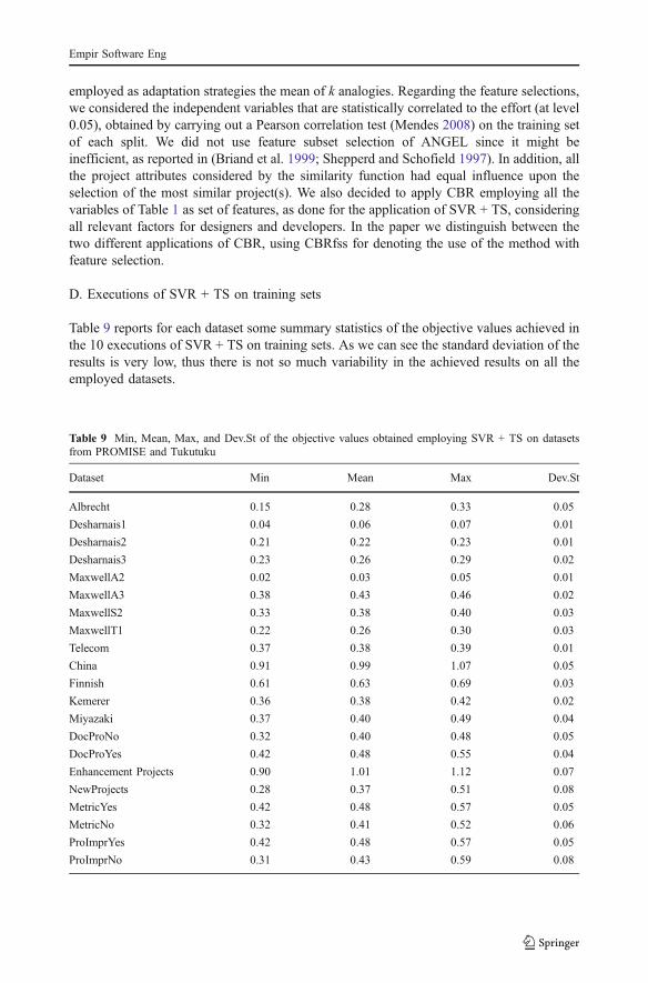
employed as adaptation strategies the mean of k analogies. Regarding the feature selections,we considered the independent variables that are statistically correlated to the effort (at level0.05), obtained by carrying out a Pearson correlation test (Mendes 2008) on the training setof each split. We did not use feature subset selection of ANGEL since it might beinefficient, as reported in (Briand et al. 1999; Shepperd and Schofield 1997). In addition, allthe project attributes considered by the similarity function had equal influence upon theselection of the most similar project(s). We also decided to apply CBR employing all thevariables of Table 1 as set of features, as done for the application of SVR + TS, consideringall relevant factors for designers and developers. In the paper we distinguish between thetwo different applications of CBR, using CBRfss for denoting the use of the method withfeature selection.
D. Executions of SVR + TS on training sets
Table 9 reports for each dataset some summary statistics of the objective values achieved inthe 10 executions of SVR + TS on training sets. As we can see the standard deviation of theresults is very low, thus there is not so much variability in the achieved results on all theemployed datasets.
Table 9 Min, Mean, Max, and Dev.St of the objective values obtained employing SVR + TS on datasetsfrom PROMISE and Tukutuku
Dataset Min Mean Max Dev.St
Albrecht 0.15 0.28 0.33 0.05
Desharnais1 0.04 0.06 0.07 0.01
Desharnais2 0.21 0.22 0.23 0.01
Desharnais3 0.23 0.26 0.29 0.02
MaxwellA2 0.02 0.03 0.05 0.01
MaxwellA3 0.38 0.43 0.46 0.02
MaxwellS2 0.33 0.38 0.40 0.03
MaxwellT1 0.22 0.26 0.30 0.03
Telecom 0.37 0.38 0.39 0.01
China 0.91 0.99 1.07 0.05
Finnish 0.61 0.63 0.69 0.03
Kemerer 0.36 0.38 0.42 0.02
Miyazaki 0.37 0.40 0.49 0.04
DocProNo 0.32 0.40 0.48 0.05
DocProYes 0.42 0.48 0.55 0.04
Enhancement Projects 0.90 1.01 1.12 0.07
NewProjects 0.28 0.37 0.51 0.08
MetricYes 0.42 0.48 0.57 0.05
MetricNo 0.32 0.41 0.52 0.06
ProImprYes 0.42 0.48 0.57 0.05
ProImprNo 0.31 0.43 0.59 0.08
Empir Software Eng
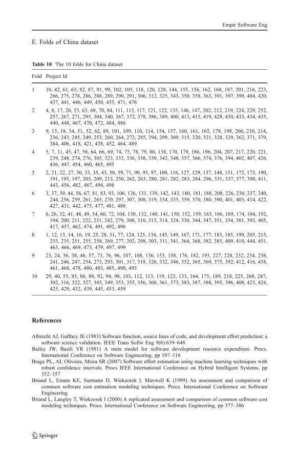
E. Folds of China dataset
References
Albrecht AJ, Gaffney JE (1983) Software function, source lines of code, and development effort prediction: asoftware science validation. IEEE Trans Softw Eng 9(6):639–648
Bailey JW, Basili VR (1981) A meta model for software development resource expenditure. Procs.International Conference on Software Engineering, pp 107–116
Braga PL, AL Oliveira, Meira SR (2007) Software effort estimation using machine learning techniques withrobust confidence intervals. Procs IEEE International Conference on Hybrid Intelligent Systems, pp352–357
Briand L, Emam KE, Surmann D, Wiekzorek I, Maxwell K (1999) An assessment and comparison ofcommon software cost estimation modeling techniques. Procs. International Conference on SoftwareEngineering
Briand L, Langley T, Wiekzorek I (2000) A replicated assessment and comparison of common software costmodeling techniques. Procs. International Conference on Software Engineering, pp 377–386
Table 10 The 10 folds for China dataset
Fold Project Id
1 10, 42, 61, 65, 82, 87, 91, 99, 102, 105, 118, 120, 128, 144, 155, 156, 162, 168, 187, 201, 216, 223,266, 275, 278, 286, 288, 289, 290, 291, 306, 312, 325, 343, 350, 358, 363, 391, 397, 399, 404, 420,437, 441, 446, 449, 450, 455, 471, 476
2 4, 8, 17, 20, 53, 63, 68, 70, 84, 111, 115, 117, 121, 122, 135, 146, 147, 202, 212, 219, 224, 229, 252,257, 267, 271, 295, 304, 340, 367, 372, 378, 386, 389, 400, 413, 415, 419, 428, 430, 433, 434, 435,440, 448, 467, 470, 472, 484, 486
3 9, 15, 18, 34, 51, 52, 62, 89, 101, 109, 110, 114, 154, 157, 160, 161, 165, 178, 198, 206, 210, 214,236, 243, 245, 249, 253, 260, 264, 272, 285, 294, 299, 309, 315, 320, 321, 328, 329, 362, 371, 379,384, 406, 418, 421, 438, 452, 464, 489
4 5, 7, 11, 45, 47, 58, 64, 66, 69, 74, 75, 78, 79, 80, 138, 170, 179, 186, 196, 204, 207, 217, 220, 221,239, 248, 274, 276, 305, 323, 333, 336, 338, 339, 342, 348, 357, 366, 374, 376, 394, 402, 407, 426,436, 447, 454, 460, 465, 495
5 2, 21, 22, 27, 30, 33, 35, 43, 50, 59, 71, 90, 95, 97, 100, 116, 127, 129, 137, 148, 151, 172, 173, 190,191, 195, 197, 203, 209, 213, 250, 262, 263, 280, 281, 282, 283, 284, 296, 331, 337, 377, 398, 411,443, 456, 482, 487, 494, 498
6 3, 37, 39, 44, 56, 67, 81, 83, 93, 106, 126, 131, 139, 142, 143, 180, 181, 188, 208, 226, 230, 237, 240,244, 256, 259, 261, 265, 270, 297, 307, 308, 319, 334, 335, 359, 370, 380, 390, 401, 403, 414, 422,427, 431, 442, 475, 477, 481, 488
7 6, 26, 32, 41, 48, 49, 54, 60, 72, 104, 130, 132, 140, 141, 150, 152, 159, 163, 166, 169, 174, 184, 192,194, 200, 211, 222, 231, 242, 279, 300, 310, 313, 314, 324, 330, 344, 347, 351, 354, 381, 393, 405,417, 457, 462, 474, 491, 492, 496
8 1, 12, 13, 14, 16, 19, 25, 28, 31, 77, 124, 125, 134, 145, 149, 167, 171, 177, 183, 185, 199, 205, 215,233, 235, 251, 255, 258, 269, 277, 292, 298, 303, 311, 341, 364, 368, 382, 385, 409, 410, 444, 451,463, 466, 469, 473, 479, 497, 499
9 23, 24, 36, 38, 46, 57, 73, 76, 96, 107, 108, 136, 153, 158, 176, 182, 193, 227, 228, 232, 234, 238,241, 246, 247, 254, 273, 293, 301, 317, 318, 326, 332, 346, 352, 365, 369, 375, 392, 412, 416, 458,461, 468, 478, 480, 483, 485, 490, 493
10 29, 40, 55, 85, 86, 88, 92, 94, 98, 103, 112, 113, 119, 123, 133, 164, 175, 189, 218, 225, 268, 287,302, 316, 322, 327, 345, 349, 353, 355, 356, 360, 361, 373, 383, 387, 388, 395, 396, 408, 423, 424,425, 429, 432, 439, 445, 453, 459
Empir Software Eng
Briand L, Wieczorek I (2002) Software resource estimation. Encyclopedia of Software Engineering, pp1160–1196
Burgess CJ, Lefley M (2001) Can genetic programming improve software effort estimation? A comparativeevaluation. Inf Softw Technol 43(14):863–873
Chang C-C, Lin C-J (2001) LIBSVM: a library for support vector machines. Software available at http://www.csie.ntu.edu.tw/~cjlin/libsvm
Cherkassky V, Ma Y (2004) Practical selection of SVM parameters and noise estimation for SVMRegression. Neural Netw 17(1):113–126
Chiu N-H, Huang S-J (2007) The adjusted analogy-based software effort estimation based on similaritydistances. J Syst Software 80(4):628–640
Conte SD, Dunsmore HE, Shen VY (1986) Software engineering metrics and model. Benjamin-CumminsPub Co, Inc. Redwood City, CA, USA
Conover WJ (1998) Practical nonparametric statistics, 3rd edn. Wiley, New YorkCook RD (1977) Detection of influential observations in linear regression. Technometrics 19:15–18Corazza A, Di Martino S, Ferrucci F, Gravino C, Mendes E (2009) Applying support vector regression for
web effort estimation using a cross-company dataset. Procs. Empirical Software Engineering andMeasurement, pp 191–202
Corazza A, Di Martino S, Ferrucci F, Gravino C, Mendes E (2011) Investigating the use of Support VectorRegression for Web Effort Estimation. Empir Softw Eng 16(2):211–243
Corazza A, Di Martino S, Ferrucci F, Gravino C, Sarro F, Mendes E (2010) How effective is Tabu search toconfigure support vector regression for effort estimation? Procs. International Conference on PredictiveModels in Software Engineering, 4
Cortes C, Vapnik V (1995) Support-vector networks. Machine Learning, 20Costagliola G, Di Martino S, Ferrucci F, Gravino C, Tortora G, Vitiello G (2006) Effort estimation modeling
techniques: a case study for web applications. Procs. International Conference on Web Engineering, pp9–16
Cristianini N, Shawe-Taylor J (2000) An introduction to support vector machines and other kernel-basedlearning methods. Cambridge University Press, New York, NY, USA
Desharnais JM (1989) Analyse statistique de la productivitie des projets in formatique a partie de latechnique des point des fonction, Ph.D. thesis, Unpublished Masters Thesis, University of Montreal
Di Martino S, Ferrucci F, Gravino C, Mendes E (2007) comparing size measures for predicting webapplication development effort: a case study. Procs. Empirical Software Engineering and Measurement,pp 324–333
Ferrucci F, Gravino C, Oliveto R, Sarro F (2009) Using Tabu search to estimate software development effort.Procs. International Conferences on Software Process and Product Measurement. LNCS 5891. Springer-Verlag, Berlin-Heidelberg, pp 307–320
Ferrucci F, Gravino C, Mendes E, Oliveto R, Sarro F (2010) Investigating Tabu search for web effort estimation.Procs. EUROMICRO Conference on Software Engineering and Advanced Applications, pp 350–357
Glover F, Laguna M (1997) Tabu search. Kluwer Academic Publishers, BostonHsu C-W, Chang C-C, Lin C-J (2010) A practical guide to support vector classification, available at http://
www.csie.ntu.edu.tw/\~cjlin/papers/guide/guide.pdfHall M, Frank E, Holmes G, Pfahringer B, Reutemann P, Witten IH (2009) The WEKA data mining
software: an update. SIGKDD Explorations 11(1), ACM New York, NY, USA, pp 10–18Hofmann T, Schölkopf B, Smola AJ (2008) Kernel methods in machine learning. Ann Stat 36:1171–1220Jeffery R, Ruhe M, Wieczorek I (2000) A comparative study of two software development cost modeling
techniques using multi-organizational and company-specific data. Inf Softw Technol 42:1009–1016Kemerer CF (1987) An empirical validation of software cost estimation models. Commun ACM 30(5):416–
429Keerthi S (2002) Efficient tuning of SVM hyper-parameters using radius/margin bound and iterative
algorithms. IEEE Trans Neural Netw 13(5):1225–1229Keerthi S, Lin C-J (2003) Asymptotic behaviors of support vector machines with Gaussian Kernel. Neural
Comput 15:1667–1689Kitchenham BA, Mendes E, Travassos GH (2007) Cross versus within-company cost estimation studies: a
systematic review. IEEE Trans Softw Eng 33(5):316–329Kitchenham B, Pickard LM, MacDonell SG, Shepperd MJ (2001) What accuracy statistics really measure.
IEE Proceedings Software 148(3):81–85Kitchenham BA, Mendes E (2004) A comparison of cross-company and single-company effort
estimation models for web applications. Procs. Evaluation & Assessment in Software Engineering,pp 47–55
Empir Software Eng
Kitchenham BA, Mendes E (2009) Why comparative effort prediction studies may be invalid. Procs.International Conference on Predictor Models in Software Engineering
Kitchenham BA (1998) A procedure for analyzing unbalanced datasets. IEEE Trans Softw Eng 24(4):278–301Kitchenham BA, Pickard L, Peeger S (1995) Case studies for method and tool evaluation. IEEE Softw 12
(4):52–62Kocaguneli E, Gay G, Menzies T, Yang Y, Keung JW (2010) When to use data from other projects for effort
estimation. Procs. IEEE/ACM international conference on Automated Software Engineering, pp 321–324
Kwok JT, Tsang IW (2003) Linear dependency between ε and the input noise in ε-support vector regression.IEEE Trans Neural Netw 14(3):544–553
Lefley M, Shepperd MJ (2003) Using genetic programming to improve software effort estimation based ongeneral datasets. Procs. GECCO, LNCS 2724, Springer-Verlag, Berlin, Heidelberg, pp 2477–2487
Li YF, Xie M, Goh TN (2009) A study of project selection and feature weighting for analogy based softwarecost estimation. J Syst Software 82(2):241–252
Mair C, Shepperd M (2005) The consistency of empirical comparisons of regression and analogy-basedsoftware project cost estimation. Procs ISESE, pp 509–518
Mattera D, Haykin S (1999) Support vector machines for dynamic reconstruction of a chaotic system. In:Scholkopf B, Burges J, Smola A (eds) Advances in kernel methods: support vector machine. MIT,Cambridge
Maxwell (2002) Applied statistics for software managers. Software Quality Institute Series, PrenticeHall, Upper Saddle River, NJ, USA
Maxwell K, Wassenhove LS, Dutta S (1999) Performance evaluation of general and company specificmodels in software development effort estimation. Manag Sci 45(6):787–803
Mendes E (2008) The use of bayesian networks for web effort estimation: further investigation. Procs.International Conference on Web Engineering, pp 203–216
Mendes E, Pollino C, Mosley N (2009) Building an expert-based web effort estimation model usingBayesian Networks Procs EASE Conference, pp 1–10
Mendes E (2009) Web cost estimation and productivity benchmarking. ISSSE, LNCS 5413, Publisher:Springer-Verlag, Berlin Heidelberg, pp 194–222
Mendes E, Mosley N, Counsell S (2005a) Investigating web size metrics for early web cost estimation. J SystSoftware 77(2):157–172
Mendes E, Di Martino S, Ferrucci F, Gravino C (2008) Cross-company vs. single-company web effortmodels using the Tukutuku database: an extended study. J Syst Software 81(5):673–690
Mendes E, Mosley N, Counsell S (2003a) Investigating early web size measures for web cost estimationProcs. Evaluation and Assessment in Software Engineering, pp 1–22
Mendes E, Kitchenham BA (2004) Further Comparison of cross-company and within-company effortestimation models for web applications. Procs. IEEE International Software Metrics Symposium, pp348–357
Mendes E, Counsell S, Mosley N, Triggs C, Watson I (2003b) Comparative study of cost estimation modelsfor web hypermedia applications. Empir Softw Eng 8(23):163–196
Mendes E, Mosley N, Counsell S (2005b) The need for web engineering: an introduction, web engineering.In: Mendes E, Mosley N (eds). Springer-Verlag, pp 1–28
Miyazaki Y, Terakado M, Ozaki K, Nozaki H (1994) Robust regression for developing software estimationmodels. J Syst Softw 27(1):3–16
Moser R, Pedrycz W, Succi G (2007) Incremental effort prediction models in agile development using radialbasis functions. Procs. International Conference on Software Engineering and Knowledge Engineering,pp 519–522
Oliveira ALI (2006) Estimation of software project effort with support vector regression. Neurocomputing 69(13–15):1749–1753
PROMISE (2011) Repository of empirical software engineering data. http://promisedata.org/repositoryShepperd MJ, Kadoda G (2001) Using simulation to evaluate prediction techniques. Procs. IEEE
International Software Metrics Symposium, pp 349–358Shepperd M, Schofield C (1997) Estimating software project effort using analogies. IEEE Trans Softw Eng
23(11):736–743Shepperd M, Schofield C, Kitchenham BA (1996) Effort estimation using analogy. Procs. International
Conference on Software Engineering, pp 170–178Shin M, Goel AL (2000) Empirical data modeling in software engineering using radical basis functions.
IEEE Trans Softw Eng 26(6):567–576Scholkopf B, Smola A (2002) Learning with Kernels. MIT Press
Empir Software Eng

Schölkopf B, Sung K, Burges C, Girosi F, Niyogi P, Poggio T, Vapnik V (1997) Comparing support vectormachines with Gaussian Kernels to radial basis function classifiers. IEEE Trans Signal Process 45(11):2758–2765
Shukla KK (2000) Neuro-genetic prediction of software development effort. Inf Softw Technol 42(10):701–713
Smola AJ, Schölkopf B (2004) A tutorial on support vector regression. Stat Comput 14(3):199–222Vapnik V, Chervonenkis A (1964) A note on one class of perceptrons. Automatics and Remote Control 25Vapnik V, Chervonenkis AY (1974) Theory of pattern recognition (in Russian). Nauka, MoscowVapnik V (1995) The nature of statistical learning theory. Springer-VerlagWieczorek I, Ruhe M (2002) How valuable is company-specific data compared to multi-company data for
software cost estimation? Procs. International Software Metrics Symposium, pp 237–246
Anna Corazza received the Laurea Degree in Electronic Engineering in 1989 and the PhD in 1996 at theUniversity of Padua, Italy. Since 1989 to 2000, she worked as researcher at the ITC-irst (now FBK) inTrento, and afterwards for three years at the University of Milan. Since 2003, she is assistant professor at theUniversity “Federico II” in Naples, Italy. Her research interests focus on statistical models and machinelearning applied to speech and natural language processing, bioinformatics, and information retrieval.
Sergio Di Martino received the PhD in Computer Science from the University of Salerno (Italy) in 2005. Hehas worked for many years as consultant for different Research Centres and Institutions. Since 2007 he isAssistant Professor at University “Federico II” in Naples, Italy. His research interests focus on knowledgediscovery and visualization from complex datasets, such as software repositories. He has published morethan 60 papers on these topics in international journals, books, and conference proceedings.
Empir Software Eng

Filomena Ferrucci is Professor of Computer Science at the University of Salerno, Italy. She is Program co-chair of the International Summer School on Software Engineering and she was Program co-chair of the 14thInternational Conference on Software Engineering and Knowledge Engineering. Her main research interestsinclude empirical software engineering, software development effort estimation, software-developmentenvironments, and Human-Computer Interaction. On these topics she has published about 150 refereedpapers in international journals, books, and conference proceedings.She was co-editor of two books andguest editor of two special issues.
Gravino Carmine received the Laurea degree in Computer Science (cum laude) in 1999, and his PhD inComputer Science from the University of Salerno (Italy) in 2003. Since march 2006 he is assistant professorin the Department of Mathematics and Informatics at the University of Salerno. His research interests includesoftware metrics and techniques to estimate web application development effort, software-developmentenvironments, design pattern recovery from object-oriented code, evaluation and comparison of notations,methods, and tools supporting software development and maintenance. He has published more than 50papers on these topics in international journals, books, and conference proceedings.
Empir Software Eng

Federica Sarro received the Laurea (summa cum laude) in Computer Science from the University of Salerno(Italy) in 2009. She is currently a PhD student at the same university. Her research activity is mainly focusedon the definition and the empirical evaluation of search based-approaches for predictive modeling in thecontexts of software development effort estimation and fault prediction. Her research interests also includefunctional metrics for sizing software products.
Emilia Mendes is Associate Professor in Information Technology at Zayed University (UAE). She has activeresearch interests in the areas of Empirical Web & Software Engineering, Evidence-based research,Hypermedia, Computer Science & Software Engineering education, in which areas she has published widelyand over 150 refereed publications, which include two books (one edited (2005) and one authored (2007)).Prof. Mendes is on the editorial board of the Software Quality Journal, International Journal of WebEngineering and Technology, the Journal of Web Engineering, the Journal of Software Measurement, theInternational Journal of Software Engineering and Its Applications, and the Advances in SoftwareEngineering Journal.
Empir Software Eng