using self-organizing maps to visualize high-dimensional data

ARTICLE IN PRESS

0098-3004/$ - se

doi:10.1016/j.ca

�Autometric1330 Inverness

USA. Tel.: +1

E-mail addr

Computers & Geosciences 31 (2005) 531–544

www.elsevier.com/locate/cageo

Using self-organizing maps to visualize high-dimensional data

Brian S. Penn�

Pan-American Center for Earth & Environmental Studies, Department of Geological Sciences, University of Texas at El Paso, El Paso,

TX 79938, USA

Received 17 August 2003; received in revised form 26 August 2004; accepted 8 October 2004

Abstract

Understanding relationships in high-dimension datasets requires proper data visualization. Two examples of high-

dimension data are major-element geochemical and hyperspectral data. Major-element geochemical data consists of

eleven oxide measurements for each sample. Well-known correlations exist for these types of data, i.e., the negative

relationship between SiO2 and MgO; other more subtle relationships are rarely apparent. Hyperspectral data is by

definition high-dimension data consisting of upwards of 100+ discrete measurements of the electromagnetic spectrum

for a material. Hyperspectral data are a significant challenge to interpret when evaluating information for

heterogeneous materials such as rocks. Self-organizing maps (SOMs) provide insight into complex relationships in

high-dimension datasets while preserving the inherent topological relations and simultaneously producing a statistical

model of the dataset. Another benefit of SOMs is their generation of composite vectors which can be analyzed to extract

the relative importance of each component during classification. The veracity of SOMs is demonstrated using two

datasets from the Spanish peaks intrusive complex of south-central Colorado including major-element geochemical and

hyperspectral measurements.

r 2004 Elsevier Ltd. All rights reserved.

Keywords: Self organizing maps; Exemplar; Major-element geochemistry; Hyperspectral

1. Introduction

Earth scientists are faced with increasing amounts of

data to sift through to extract meaningful information.

Much of the analysis process is successfully performed

using basic statistical methods, but often subtle relation-

ships within a dataset do not lend themselves to

standard statistical approaches. At this point simple

visualization may be appropriate. While simple visuali-

zation approaches are sufficient for datasets with low

dimensionality, complex datasets, i.e., high-dimensional,

e front matter r 2004 Elsevier Ltd. All rights reserve

geo.2004.10.009

Inc.-A Business Unit of the Boeing Company,

Drive, Suite 350, Colorado Springs, CO 80910,

719 572 8142; fax: +1 719 637 8535.

ess: [email protected].

are difficult to visualize. An approach is needed that is

both unbiased and visually accessible. Self-organizing

maps (SOMs) fulfill these requirements. SOMs, which

share similarities with vector quantization (Gray, 1984;

Kohonen, 1990; Hammer and Villmann, 2002), were

first described in detail by Kohonen (1981, 1982). Since

then they have been applied in numerous fields ranging

including financial markets (Deboeck, 1998; Deboeck

and Kohonen, 1998), data mining (Bigus, 1996; Vesanto

and Alhoniemi, 2000), robotics (Takahashi et al., 2001),

and hyperspectral image classification and anomaly

detection (Penn, 2002a, b; Penn and Wolboldt, 2003).

Two scenarios are presented here involving high

dimensional datasets: major-element geochemical data

and hyperspectral signatures. The major-element data

are from a number of different published sources and

d.

www.elsevier.com/locate/cageo

ARTICLE IN PRESSB.S. Penn / Computers & Geosciences 31 (2005) 531–544532

the hyperspectral signatures were collected using a

handheld spectrometer. Each scenario is discussed in

detail below, but first visualization and the technique of

using SOMs are introduced.

2. Data visualization

Visualizing multidimensional data is critical to under-

standing complex relationships in natural systems.

Unfortunately, the human brain is only capable of

simultaneously visualizing three or four dimensions. To

understand natural systems, data from diverse sources

must be integrated in a manner comprehensible for

human interpretation. In geology it is common to

present data in a graphical format. These data are

usually limited to three-dimensions or less permitt-

ing easy visualization through standard graphing

techniques. As the dimensionality of the data increa-

ses, the complexity of visualizing relationships also

increases.

Examining datasets with fewer than four dimensions

is usually handled by standard graphical software

packages or spreadsheets. For example: one-dimen-

sional data such as point readings, e.g., density,

temperature, etc., can be graphed as a series of

independent values with another measurable quantity

related to it or simply as a number sequence. Two-

dimensional data sets are easily displayed via a scatter

plot with the independent variable on the abscissa (x)

and the dependent variable on the ordinate (y) axis.

Adding the third dimension is relatively easy as most

graphics packages can generate perspective graphs of

three-dimensional data. This approach quickly degen-

erates for datasets with dimensionalities beyond three. If

the data are spatial in nature they can be imported into a

geographic information system (GIS) and projected into

two-dimensions. Unfortunately, many datasets have

critical aspects that do not lend themselves to a simple

implementation in a GIS.

Before data from multiple diverse sources can be

integrated into a coherent picture, methods for integrat-

ing and visualizing high-dimensionality data from

homogenous sources must be demonstrated. A simple

method to visualize data with dimensionalities greater

than three involves projecting the information from a

higher dimension down to two- or three-dimensional

space. It is common to visualize three-dimensions by

projecting the data into two dimensions, i.e., three-

dimension graphs of data points on to a two-dimen-

sional sheet of paper. What is not often seen is the

projection of four or more dimensions into two-

dimensional space. Unless great care is taken this

approach does not always maintain the inherent

topological relationships in the dataset. It is also

desirable to have an automated process that is both

objective and maintains the topology of the original

data. SOMs are presented here is as a technique for

visualizing multidimensional data in ways that reveal

interesting relationships not obvious from direct exam-

ination.

3. Self-organizing maps

Neural networks (NNs) represent a shift in the

research of how to get computers to think like human

beings. From the 1940s–1960s certain lines of research in

artificial intelligence dealing with computer hardware

focused on developing systems loosely based on neurons

in the human brain. This line of research showed

promise until Minsky and Papert (1969) demonstrated

that perceptrons, or two-layer NNs, are unable to

distinguish linearly inseparable relationships such as the

XOR function.

Although Minsky and Papert demonstrated this

weakness of separability for one particular type of

NN, less than five years later Werbos (1974) defined a

method for circumventing this problem using NNs with

multiple layers. Nonetheless, it was nearly 20 years

before vigorous NN research began again.

SOMs are a type of neural network described by

Tuevo Kohonen (1981, 1982, 1990, 2001). SOMs

operate on real vectors much like the codebook vectors

of classical vector quantization (Gersho, 1979; Zador,

1982; Gray, 1984). SOMs partition the search space into

Voronoi sets. A Veronoi set is a set of all input vectors

that share a common distance (Euclidian, spectral angle,

Pearson’s correlation, etc.) from a model vector

(Kohonen, 2000).

SOMs are also a method for dimensionality reduction

(Carpenter et al., 1997; Merenyi, 1998; Villman and

Merenyi, 2001). SOMs create prototypical vectors

representing a dataset while maintaining topological

relationships inherent in the dataset. These relationships

are then projected to lower dimension-space (1- or 2-d)

for ease of visualization (Vesanto and Alhoniemi, 2000).

As originally conceived, SOMs are a nonlinear projec-

tion method for orderly mapping an n-dimensional

space’s manifold on to an n-dimensional (usually 2

dimensional) regular grid (Kohonen, 1982, 2001).

As with other NNs, SOMs are useful because they are

a computationally efficient, reproducible non-para-

metric approach to exploring relationships with data-

sets. One of the chief distinctions between ‘‘classical’’

NNs and SOMs is their ability to perform unsupervised

learning. SOMs require no a priori information to

function and they excel at establishing unseen relation-

ships in datasets (Deboeck, 1998; Penn, 2002a,b). Once a

SOM is trained for a specific dataset, it can be applied to

other similar datasets. SOM-created vectors for hyper-

spectral data sets can then be used in a fashion similar to

ARTICLE IN PRESSB.S. Penn / Computers & Geosciences 31 (2005) 531–544 533

codebooks used in vector quantization to classify

subsequent imagery data.

Another salient feature of SOMs is their ability to

preserve a dataset’s topology (Villmann et al., 1997).

Topology is the geometry of data sets. This is the desired

result when working with high-dimension data. A second

benefit of SOMs is their ability to automatically generate

a statistical model of any dataset (Caudill, 1988).

In Penn and Livo (2001), SOMs were used to map

surface geology in south-central New Mexico which

correlated well with available geologic maps of the area.

Additional investigation demonstrated the ability of

SOMs to quickly identify anomalies and end-members

for hyperspectral unmixing algorithms (Munoz and

Muruzabal, 1998; Penn, 2002a, b).

SOMs are also capable of extracting relationships

from disparate data sets and identifying cogent relation-

ships within datasets (Tzafestas and Anthopoulos, 1997;

Wan and Fraser, 1999; Sbarbaro and Johansen, 2002;

Kohonen and Somervuo, 1998, Brodaric, et al., 2004).

Kohonen (1996) pointed out that any set with definable

distance metrics can be mapped using a SOM.

A SOM is composed of an n-dimensional array of

nodes. Each node is initialized as a random unit vector

in n-dimensional space. Each input vector is normalized

by dividing each vector element by the sum of all vector

elements. After normalization the multi-dimensional

data is presented to each of the individual nodes. Using

a ‘‘winner-take-all’’ selection rule, the node whose vector

most closely matches the input data is found. This

winning vector incorporates, or adjusts, its vector

weights to match the input data. Vectors in the nodes

surrounding the winning node are modified so that they

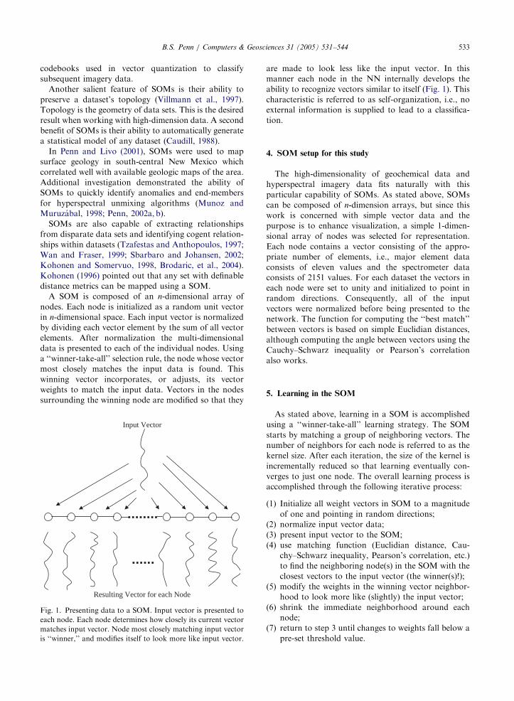
Input Vector

Resulting Vector for each Node

Fig. 1. Presenting data to a SOM. Input vector is presented to

each node. Each node determines how closely its current vector

matches input vector. Node most closely matching input vector

is ‘‘winner,’’ and modifies itself to look more like input vector.

are made to look less like the input vector. In this

manner each node in the NN internally develops the

ability to recognize vectors similar to itself (Fig. 1). This

characteristic is referred to as self-organization, i.e., no

external information is supplied to lead to a classifica-

tion.

4. SOM setup for this study

The high-dimensionality of geochemical data and

hyperspectral imagery data fits naturally with this

particular capability of SOMs. As stated above, SOMs

can be composed of n-dimension arrays, but since this

work is concerned with simple vector data and the

purpose is to enhance visualization, a simple 1-dimen-

sional array of nodes was selected for representation.

Each node contains a vector consisting of the appro-

priate number of elements, i.e., major element data

consists of eleven values and the spectrometer data

consists of 2151 values. For each dataset the vectors in

each node were set to unity and initialized to point in

random directions. Consequently, all of the input

vectors were normalized before being presented to the

network. The function for computing the ‘‘best match’’

between vectors is based on simple Euclidian distances,

although computing the angle between vectors using the

Cauchy–Schwarz inequality or Pearson’s correlation

also works.

5. Learning in the SOM

As stated above, learning in a SOM is accomplished

using a ‘‘winner-take-all’’ learning strategy. The SOM

starts by matching a group of neighboring vectors. The

number of neighbors for each node is referred to as the

kernel size. After each iteration, the size of the kernel is

incrementally reduced so that learning eventually con-

verges to just one node. The overall learning process is

accomplished through the following iterative process:

(1)
Initialize all weight vectors in SOM to a magnitude
of one and pointing in random directions;

(2)
normalize input vector data;
(3)
present input vector to the SOM;
(4)
use matching function (Euclidian distance, Cau-
chy–Schwarz inequality, Pearson’s correlation, etc.)

to find the neighboring node(s) in the SOM with the

closest vectors to the input vector (the winner(s)!);

(5)
modify the weights in the winning vector neighbor-
hood to look more like (slightly) the input vector;

(6)
shrink the immediate neighborhood around each
node;

(7)
return to step 3 until changes to weights fall below a
pre-set threshold value.


6. Geochemical data example

The spanish peaks are a middle-oligocene to early-

miocene transitional intrusive center, i.e., total akali-

silica (TAS) compositions straddle the division between

alkaline to sub-alkaline, located in south-central Color-

ado (see: http://www.spanishpeakscolorado.com and

(Penn and Butler, 2000), for more background). High-

precision 40Ar/39Ar dates indicate nearly continuous

intrusive activity from 26.6 to 21.8Ma for the Spanish

peaks region. The intrusive activity in the Spanish peaks

is divided into three distinct geochemical phases: early

alkaline, middle sub-alkaline, and late alkaline. The

earliest intrusive magmas are comprised of mostly dikes

and sills of alkaline basalts and lamprophyres (campto-

nites). Lamprophyres are porphyritic mafic rocks with

phenocrysts composed exclusively of mafic minerals, i.e.,

olivine, pyroxene, hornblende, biotite and phlogopite

and a groundmass consisting of both mafic and felsic

minerals. Amphiboles are the primary mafic phenocryst

phase in camptonites. During the middle intrusive phase

sub-alkaline rocks were emplaced including the stocks of

the west and east Spanish peaks along with numerous

radial dikes consisting mostly of monzonite and

syenite porphyries. Interestingly, west Spanish peak

is composed of a phaneritic (one grain-size) quartz

syenite; east Spanish peak is comprised of two stocks,

an inner granite porphyry and an outer stock of

granodiorite porphyry. The last, or latest, phase of

intrusive activity again involved alkaline magmas

including minettes, mostly as dikes and sills. Minettes

are shoshonitic (calc-alkaline) lamprophyres with a

dominant mafic phenocryst phase of biotite and

phlogopite micas.

Major-element analysis of geochemical data is often

overlooked in the development of petrogenetic models

because of the high-dimensionality of the data, i.e.,

eleven components (SiO2, TiO2, Al2O3, Fe2O3, FeO,

MgO, CaO, MnO, K2O, Na2O, P2O5) and ambigui-

ties inherent in path-independent petrogenetic processes.

The primary barrier preventing researchers from inte-

grating major-element analysis into their studies is

the establishment of coherent relationships in high-

dimensional datasets. Manual methods exist for

projecting these types of datasets, but they are very

tedious.

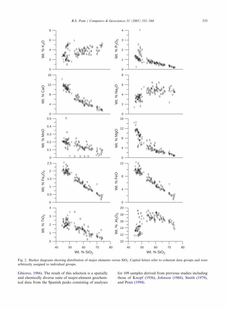
The traditional approach to viewing these compo-

nents is via Harker diagrams (Fig. 2) where SiO2 is on

the abscissa and one or more of the other major oxide

elements are graphed on the ordinate axis. Petrogenetic

interpretations based solely on Harker diagrams are

often simplistic resulting in erroneous petrogenetic

conclusions.

Other graphical approaches assume a pre-existing

petrogenetic relationship among the data. One such plot

used for igneous petrogenesis is the AFM diagram. The

AFM diagram is a ternary diagram used to plot total

alkalies (Na2O+K2O), Fe oxides (FeO+Fe2O3), and

MgO. These particular oxides are the basis for the

igneous AFM, or IAFM, diagram as opposed to the

metamorphic diagram of the same name used to plot

Al2O3–FeO–MgO space for pelitic rocks, i.e., composed

of clay minerals. The IAFM diagram is used to

distinguish between tholeiitic and calc-alkaline differ-

entiation trends in sub-alkaline magmatic series (Roll-

inson, 1993). Blindly applying an IAFM diagram to

other igneous environments leads novice researchers to

the wrong petrogenetic conclusions because their

data is not applicable to the particular type of

environment from which the diagram was derived.

Such was the case with the Spanish peaks in south-

central Colorado. Previous work in this area based

petrogenetic conclusions on the IAFM diagram

(Smith, 1979). Any evolutionary lines drawn for the

Spanish peaks based on an IAFM diagram are equivocal

because rock compositions appear to have begun as

alkaline, transitioned to sub-alkaline, then transitioned

back to alkaline. These transitions clearly violate the

idea that these samples are derived from a simple

evolutionary process because there is no known

petrogenetic process that causes magma compositions

to cross the thermal divide between alkaline and

subalkaline rocks.

Although not always possible, every attempt must be

made to ensure that major-element data is consistent

with the other geochemical data for a particular suite of

rocks. For the Spanish peaks in south-central Colorado,

previous investigators (Jahn, 1973; Smith, 1975; Jahn et

al., 1979) relied primarily on trace and radiogenic

elements to develop their petrogenetic models to the

virtual exclusion of the major-element data.

This omission led to a re-examination of the major-

element data associated with the Spanish peaks and the

development of a petrogenetic model consistent with

these data (Penn, 1994).

Thermodynamics and evidence from experimental

petrology preclude a simple evolutionary process cap-

able of yielding this diverse suite of rocks. By analyzing

the major element data in multiple dimensions, Penn

(1994) established new relationships among the data

even though the Spanish peaks had been extensively

studied for over a century (Hills, 1899, 1900, 1901;

Knopf, 1936; Johnson, 1968; Smith, 1975, 1979; Penn,

1994).

Each major-element data point from the Spanish

peaks was reviewed for consistency and possible closure

problems due to Loss on Ignition (L.O.I.) errors, etc.

The hypabyssal nature of these rocks required main-

taining consistency with respect to the relative propor-

tion of FeO to Fe2O3, i.e., Fe2+/

PFe, as such these

values were recalculated to the Fayalite–Magnetite–

Quartz (E0.85) oxygen buffer (Carmichael and

http://www.spanishpeakscolorado.com

ARTICLE IN PRESS

40 50 60 70 80

Wt. % SiO2

40 50 60 70 80

Wt. % SiO2

0

1

2

3

4

Wt.

% T

iO2

?

10

12

14

16

18

20

Wt.

% A

l 2O

3

0

0.5

1

1.5

2

2.5

Wt.

% F

e 2O

3

Wt.

% P

2O5

0

4

8

12

Wt.

% F

eO

0

0.1

0.2

0.3

0.4

0.5

Wt.

% M

nO

0

4

8

12

16W

t. %

MgO

0

4

8

12

16

Wt.

% C

aO

0

2

4

6

8

Wt.

% N

a 2O

0

2

4

6

8

Wt.

% K

2O

0

1

2

3

4

? ?

?

?

?

??

?

? BB

BB

BBBBB

B

B

B

BE

E

E

EE

FF

F

SS

SS

S

S

S

S

S S

SS

SSSS

S

S S

S S

S

S

S

S

S

SS

SSSSSS

SS

SSS

SSS

SS

TTTT

TTT T

TUUUUV

V

Z

ZZZ

ZZZ

Z

ZZZ

?

?

?

?

?

?

??

?

BB

B BBB

B

BBB

BBB

E

E

E

EE

F

F

FSS S

S

SS

S

S

S SS

SS

SS

S

SS S

S

S

S

SS S

SSS S

SS

S

S

S

S

S

SS

S

S

SS

S

STTTTTTT TT

UUU

UVV

ZZZZZZZ ZZZ

Z

?

?

?

?

?

?

?

?

?BB

BB

B

BBBB

BB

BB

EEEE

E

FF

F

SS

S

S

S

SS

S

SS

S

SSS

S

SS

S S

S

S

S

S

S

S

S

SS

S

SS

SS

S

SS

SS

S

SS

SS

S

TT

T

TTTT

TT

UUUU

VV

ZZZZ ZZ

Z

ZZ

ZZ

?

??

?

?

??

?

?

B

BBBB

BBBB

BBBB

E

E

E

E

E

FFF

SS SS

SSS S

S SSSS

S

SS

S

S SS S

S SS

SS

SS

S

SS

SSS

SS SS

S

SSSS

S

TTT

TT

TT

TT

UUU

U

VV

ZZZZ

ZZZ

Z

Z

Z

Z

?

??

?

?

?

?

?

?

BBB

B

B

B

B

BBBBBB

E

E

E

E

E

F

F

F

SS

SSS

S

S

S

S

SSS

SSS

SS

S SS S

SS

S

SS

SS

S

SS

S

S

SS

S

SS

SS SSS

S

TTTTTTT T

TUUUUVV

ZZZZ

ZZ

ZZ

ZZZ

?

?

?

?

?

?

? ?

?

BB

BBBB

B

BB

BBBB

EE

EEE

F

F

F

SS

SS

S

SS

S

S

S

S

SSS

S

SS

S

SS

S

S SS

SS

SSS

SSSS

SSS

SS

S

SSSS

S

TTTTTTT

TTUUUUVV

ZZZZ

ZZZZZ

ZZ?

??

??

?

??

?

BBB

BBBBBBB

BBB

EE

EE

EF

F

F

S

S SS

SSS

S

S

S

SSSSS S

S

SS

S SS SS SSSS S

SS

S

S

S

SS S

S

SS

S

SS

ST

T

T

TTTT

TT UUUU

VV

Z

ZZ

ZZZ

ZZZZZ

?

?

??

?

?

?

?

?

B

BB B

BBBBB

BBB

B

EEE

E

E

FF

F

SS S

SS

SSS

S

S

S

SSS

S

S

S

S S

S

S

SS

S S

S

SSS

SS

SS

SS

S S

S

S

S

SSS

S

TT

TTTT

TTT

UUU

UVV

ZZZZ

ZZ

ZZ

ZZZ

?

?

?

?

?

??

?

? BBB BBBBBBBBBB

E

E

EEE

FF

F SS

SSS

SS SS S

SSS

SSS

S

S S

S SS

SS

SS

SSSSSS

S SSS SSS S

SSSS

TTTTTTT TTUUUUVV

ZZZ

Z Z

Z

ZZZ

Z

Z

?

?

?

?

?

?

?

?

?BB

BB

B

BBBB

BB

BB

EEEE

E

FF

F

SS

S

S

S

SS

S

SS

S

SSS

S

SS

S S

S

S

S

S

S

S

S

SS

S

SS

SS

S

SS

SS

S

SS

SS

S

TT

T

TTTT

TT

UUUU

VV

ZZZZ ZZ

ZZZ

ZZ

Fig. 2. Harker diagrams showing distribution of major elements versus SiO2. Capital letters refer to coherent data groups and were

arbitrarily assigned to individual groups.

B.S. Penn / Computers & Geosciences 31 (2005) 531–544 535

Ghiorso, 1986). The result of this selection is a spatially

and chemically diverse suite of major-element geochem-

ical data from the Spanish peaks consisting of analyses

for 109 samples derived from previous studies including

those of Knopf (1936), Johnson (1968), Smith (1979),

and Penn (1994).


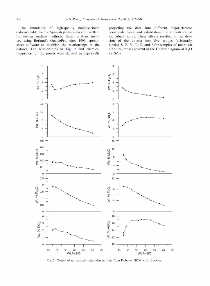
The abundance of high-quality major-element

data available for the Spanish peaks makes it excellent

for testing analysis methods. Initial analysis invol-

ved using Borland’s QuatroPro, circa 1990, spread-

sheet software to establish the relationships in the

dataset. The relationships in Fig. 2 and chemical

uniqueness of the points were derived by repeatedly

45 50 55 60 65 70 75Wt. % SiO2

0

1

2

3

4

Wt.

% T

iO2

0

0.5

1

1.5

2

2.5

Wt.

% F

e 2O

3

0

0.1

0.2

0.3

0.4

0.5

Wt.

% M

nO

0

4

8

12

16

Wt.

% C

aO

0

2

4

6

8

Wt.

% K

2O

Fig. 3. Output of normalized major element d

projecting the data into different major-element

coordinate bases and establishing the consistency of

individual points. These efforts resulted in the divi-

sion of the dataset into five groups (arbitrarily

labeled S, E, V, T, Z, and ? for samples of unknown

affinities) most apparent in the Harker diagram of K2O

vs. SiO2.

45 50 55 60 65 70 75Wt. % SiO2

10

12

14

16

18

Wt.

% A

I 2O

3

0

4

8

12

Wt.

% F

eO

0

4

8

12

16

Wt.

% M

gO

0

2

4

6

8

Wt.

% N

a 2O

0

1

2

3

4

Wt.

% P

2O5

ata from Kohonen SOM with 10 nodes.


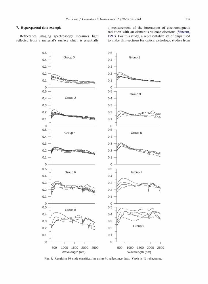
7. Hyperspectral data example

Reflectance imaging spectroscopy measures light

reflected from a material’s surface which is essentially

Group 0

Group 2

Group 4

0

0.1

0.2

0.3

0.4

0.5Group 6

500 1000 1500 2000 2500Wavelength (nm)

0

0.1

0.2

0.3

0.4

0.5

0

0.1

0.2

0.3

0.4

0.50

0.1

0.2

0.3

0.4

0.5

0

0.1

0.2

0.3

0.4

0.5

Group 8

Fig. 4. Resulting 10-node classification using %

a measurement of the interaction of electromagnetic

radiation with an element’s valence electrons (Vincent,

1997). For this study, a representative set of chips used

to make thin-sections for optical petrologic studies from

Group 1

Group 3

Group 5

Group 7

0

0.1

0.2

0.3

0.4

0.5

0

0.1

0.2

0.3

0.4

0.5

0

0.1

0.2

0.3

0.4

0.50

0.1

0.2

0.3

0.4

0.5

0

0.1

0.2

0.3

0.4

0.5

500 1000 1500 2000 2500Wavelength (nm)

Group 9

reflectance data. Y-axis is % reflectance.


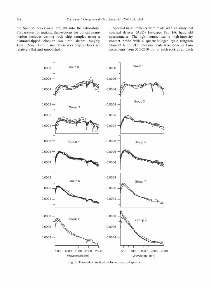
the Spanish peaks were brought into the laboratory.

Preparation for making thin-sections for optical exam-

ination includes cutting rock chip samples using a

diamond-tipped circular saw into shapes roughly

4 cm� 2 cm� 1 cm in size. These rock chip surfaces are

relatively flat and unpolished.

0.0004

0.0006

0.0008

0.0004

0.0006

0.0008

0.0004

0.0006

0.0008

0.0004

0.0006

0.0008

0.0004

0.0006

0.0008

0.

0.

0.

0.

0.

0.

0.

0.

0.

0.

0.

0.

0.

0.

0.

Group 0

Group 2

Group 4

Group 6

500 1000 1500 2000 2500

Wavelength (nm)

Group 8

Fig. 5. Ten-node classification

Spectral measurements were made with an analytical

spectral devices (ASD) Fieldspec Pro FR handheld

spectrometer. The light source was a high-intensity

contact probe with a quartz-halogen cycle tungsten

filament lamp. 2151 measurements were done in 1 nm

increments from 350–2500 nm for each rock chip. Each

0004

0006

0008

0004

0006

0008

0004

0006

0008

0004

0006

0008

0004

0006

0008

Group 1

Group 3

Group 5

Group 7

500 1000 1500 2000 2500

Wavelength (nm)

Group 9

for normalized spectra.


spectral measurement is the result averaging of 50

individual sequential measurements. All values were

converted to reflectance using Labsphere, Inc. calibrated

Spectralon (Polytetrafluoroethylene) as the white refer-

ence. A total of 61 rock chip samples were measured for

this study. Individual spectra were manually corrected to

remove offsets between the three spectrometers in the

ASD by adding corresponding offset to longer wave-

lengths. These offsets are relicts of slight variations in

responsiveness near the edges of the detectors. Modi-

fications generally were significantly less than 0.1%.

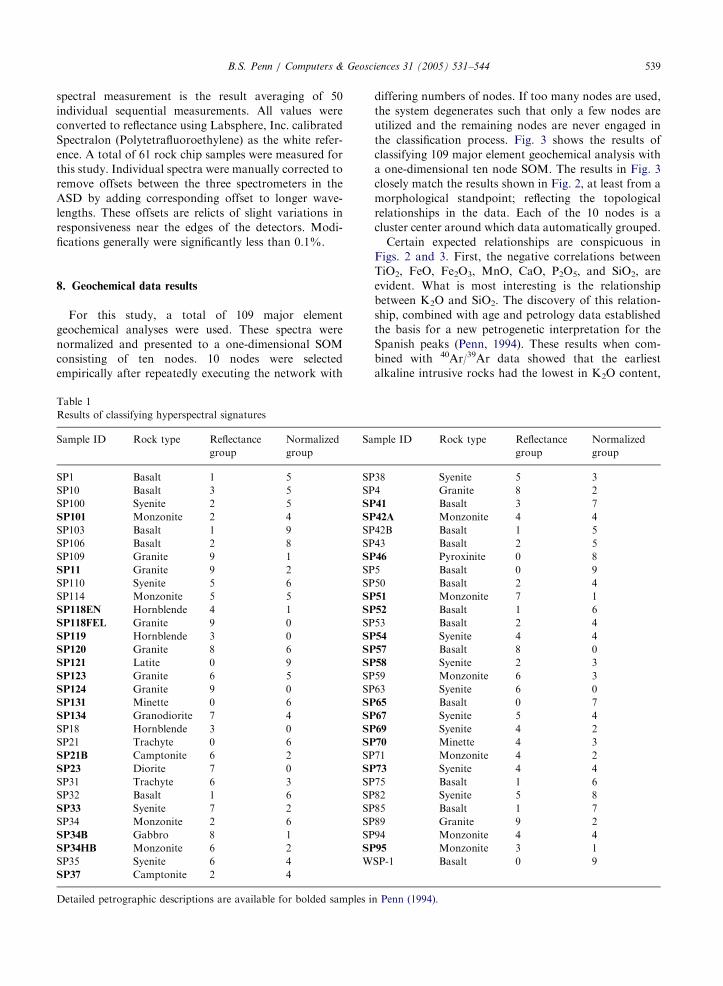
8. Geochemical data results

For this study, a total of 109 major element

geochemical analyses were used. These spectra were

normalized and presented to a one-dimensional SOM

consisting of ten nodes. 10 nodes were selected

empirically after repeatedly executing the network with

Table 1

Results of classifying hyperspectral signatures

Sample ID Rock type Reflectance

group

Normalized

group

Sa

SP1 Basalt 1 5 SP

SP10 Basalt 3 5 SP

SP100 Syenite 2 5 SP

SP101 Monzonite 2 4 SP

SP103 Basalt 1 9 SP

SP106 Basalt 2 8 SP

SP109 Granite 9 1 SP

SP11 Granite 9 2 SP

SP110 Syenite 5 6 SP


SP118EN Hornblende 4 1 SP

SP118FEL Granite 9 0 SP

SP119 Hornblende 3 0 SP


SP121 Latite 0 9 SP



SP131 Minette 0 6 SP

SP134 Granodiorite 7 4 SP

SP18 Hornblende 3 0 SP

SP21 Trachyte 0 6 SP

SP21B Camptonite 6 2 SP

SP23 Diorite 7 0 SP

SP31 Trachyte 6 3 SP

SP32 Basalt 1 6 SP

SP33 Syenite 7 2 SP


SP34B Gabbro 8 1 SP

SP34HB Monzonite 6 2 SP

SP35 Syenite 6 4 W

SP37 Camptonite 2 4

Detailed petrographic descriptions are available for bolded samples i

differing numbers of nodes. If too many nodes are used,

the system degenerates such that only a few nodes are

utilized and the remaining nodes are never engaged in

the classification process. Fig. 3 shows the results of

classifying 109 major element geochemical analysis with

a one-dimensional ten node SOM. The results in Fig. 3

closely match the results shown in Fig. 2, at least from a

morphological standpoint; reflecting the topological

relationships in the data. Each of the 10 nodes is a

cluster center around which data automatically grouped.

Certain expected relationships are conspicuous in

Figs. 2 and 3. First, the negative correlations between

TiO2, FeO, Fe2O3, MnO, CaO, P2O5, and SiO2, are

evident. What is most interesting is the relationship

between K2O and SiO2. The discovery of this relation-

ship, combined with age and petrology data established

the basis for a new petrogenetic interpretation for the

Spanish peaks (Penn, 1994). These results when com-

bined with 40Ar/39Ar data showed that the earliest

alkaline intrusive rocks had the lowest in K2O content,

mple ID Rock type Reflectance

group

Normalized

group

38 Syenite 5 3

4 Granite 8 2

41 Basalt 3 7

42A Monzonite 4 4

42B Basalt 1 5

43 Basalt 2 5

46 Pyroxinite 0 8

5 Basalt 0 9

50 Basalt 2 4

51 Monzonite 7 1

52 Basalt 1 6

53 Basalt 2 4

54 Syenite 4 4

57 Basalt 8 0

58 Syenite 2 3

59 Monzonite 6 3

63 Syenite 6 0

65 Basalt 0 7

67 Syenite 5 4

69 Syenite 4 2

70 Minette 4 3

71 Monzonite 4 2

73 Syenite 4 4

75 Basalt 1 6

82 Syenite 5 8

85 Basalt 1 7

89 Granite 9 2

94 Monzonite 4 4

95 Monzonite 3 1

SP-1 Basalt 0 9

n Penn (1994).


while the middle and late phases of intrusive activity

contained as much as 50% more K2O. While not

conclusive, this relationship suggests a possible hypoth-

esis for testing that the source for the earliest magmas

was significantly different from the later phases.

9. Hyperspectral data results

First, the reflectance spectra, then the normalized

reflectance spectra, were presented to a 10 node SOM

(Figs. 4 and 5 and Table 1). Normalization of the

spectra was achieved by dividing the measurement at

each wavelength by the sum of all the measurements.

In Fig. 4, the spectra are classified based primarily on

the percent reflectance. The groups with the lowest

reflectance values are also the most homogeneous. The

groups with the highest reflectance exhibit the largest

variation. Nonetheless, there is a general progression

from those samples with the least average percent

reflectance to those with the greatest average percent

reflectance.

Fig. 5 illustrates the results of normalizing the spectra

and presenting them to the network. These data also

show coherent variation from group to group with the

groups 0–4 exhibiting a relatively flat shape. Subsequent

groups 5–9 exhibit the development of a pronounced

increase in values at shorter wavelengths. The earlier

SiO2 TiO2 Al2O3 Fe2O3 FeO M

Major

0

2040

60

80

Wt.

%

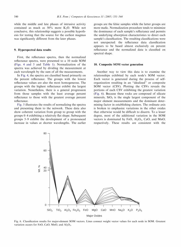
Fig. 6. Classification results for major-element SOM vectors. Lines

variation occurs for FeO, CaO, MnO, and Al2O3.

groups are the felsic samples while the latter groups are

more mafic. Normalization procedure tends to minimize

the dominance of each sample’s reflectance and permits

the underlying absorption characteristics to direct each

sample’s classification. The resulting classifications were

not unexpected: the reflectance data classification

appears to be based almost exclusively on percent

reflectance and the normalized data is classified on

spectral shape.

10. Composite SOM vector generation

Another way to view this data is to examine the

relationships exhibited by each node’s SOM vector.

Each vector is generated during the process of self-

organization resulting in an ‘‘idealized’’ or composite

SOM vector (CSV). Plotting the CSVs reveals the

portions of each CSV exhibiting the greatest variation

(Fig. 6). Because these rocks are composed of silicate

minerals, SiO2 is the single largest component of the

major element measurements and the dominant deter-

mining factor in establishing clusters. The ordinate axis

is broken to emphasize variations in the other oxides

that otherwise would be difficult to discern. To a lesser

degree, most of the additional variation in the SOM

vectors is dominated by FeO, Al2O3, CaO, and MnO;

respectively. These results are consistent with the

gO CaO MnO Na2O K2O P2O5

Oxides

connect weight vector values for each node in SOM. Greatest


current approach to classifying igneous rocks, with

the exception of the role of the alkali-oxides (K2O

and Na2O).

Several aspects are worth noting in both hyperspectral

classifications. The pronounced concavity upward sug-

gests an increasingly dominant role of Fe in controlling

the reflectance properties for the more felsic composi-

tions. This particular shape is consistent with bare soil

which is analogous to heterogeneous nature of rocks,

i.e., comprised of numerous minerals.

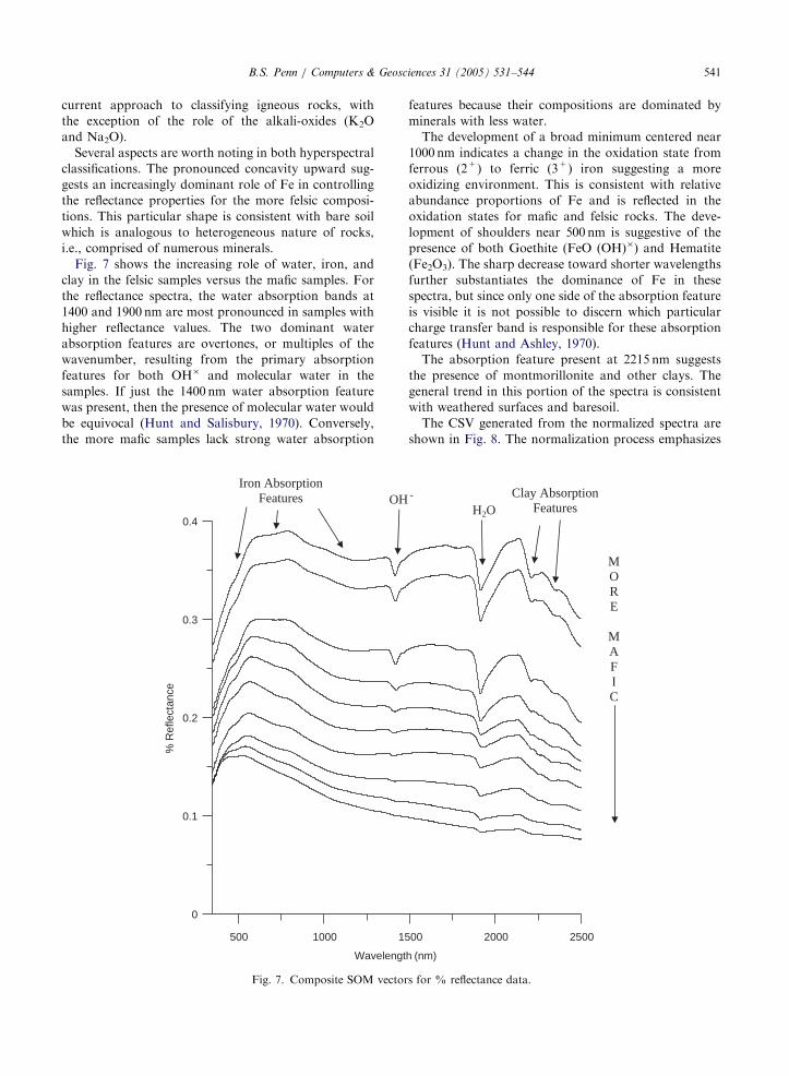
Fig. 7 shows the increasing role of water, iron, and

clay in the felsic samples versus the mafic samples. For

the reflectance spectra, the water absorption bands at

1400 and 1900 nm are most pronounced in samples with

higher reflectance values. The two dominant water

absorption features are overtones, or multiples of the

wavenumber, resulting from the primary absorption

features for both OH� and molecular water in the

samples. If just the 1400 nm water absorption feature

was present, then the presence of molecular water would

be equivocal (Hunt and Salisbury, 1970). Conversely,

the more mafic samples lack strong water absorption

500 1000 15

Wavelengt

0

0.1

0.2

0.3

0.4

% R

efle

ctan

ce

Iron Absorption Features OH

Fig. 7. Composite SOM vector

features because their compositions are dominated by

minerals with less water.

The development of a broad minimum centered near

1000 nm indicates a change in the oxidation state from

ferrous (2+) to ferric (3+) iron suggesting a more

oxidizing environment. This is consistent with relative

abundance proportions of Fe and is reflected in the

oxidation states for mafic and felsic rocks. The deve-

lopment of shoulders near 500 nm is suggestive of the

presence of both Goethite (FeO (OH)�) and Hematite

(Fe2O3). The sharp decrease toward shorter wavelengths

further substantiates the dominance of Fe in these

spectra, but since only one side of the absorption feature

is visible it is not possible to discern which particular

charge transfer band is responsible for these absorption

features (Hunt and Ashley, 1970).

The absorption feature present at 2215 nm suggests

the presence of montmorillonite and other clays. The

general trend in this portion of the spectra is consistent

with weathered surfaces and baresoil.

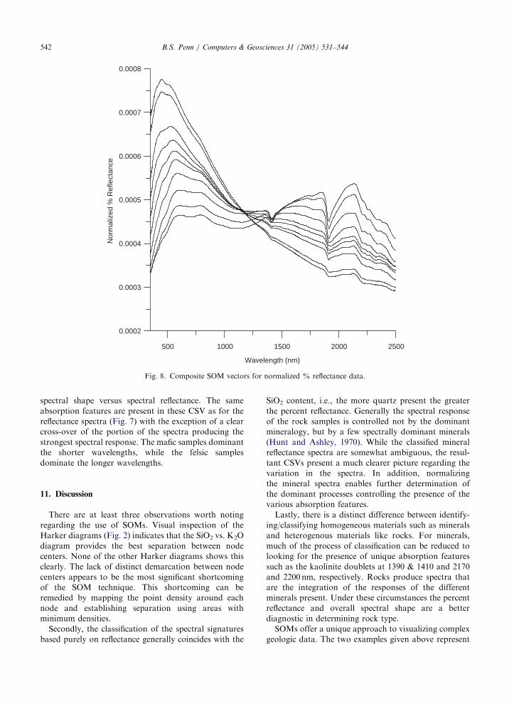
The CSV generated from the normalized spectra are

shown in Fig. 8. The normalization process emphasizes

00 2000 2500

h (nm)

H2O Clay Absorption

Features -

MORE

MAFIC

s for % reflectance data.

ARTICLE IN PRESS

500 1000 1500 2000 2500

Wavelength (nm)

0.0002

0.0003

0.0004

0.0005

0.0006

0.0007

0.0008

Nor

mal

ized

% R

efle

ctan

ce

Fig. 8. Composite SOM vectors for normalized % reflectance data.

B.S. Penn / Computers & Geosciences 31 (2005) 531–544542

spectral shape versus spectral reflectance. The same

absorption features are present in these CSV as for the

reflectance spectra (Fig. 7) with the exception of a clear

cross-over of the portion of the spectra producing the

strongest spectral response. The mafic samples dominant

the shorter wavelengths, while the felsic samples

dominate the longer wavelengths.

11. Discussion

There are at least three observations worth noting

regarding the use of SOMs. Visual inspection of the

Harker diagrams (Fig. 2) indicates that the SiO2 vs. K2O

diagram provides the best separation between node

centers. None of the other Harker diagrams shows this

clearly. The lack of distinct demarcation between node

centers appears to be the most significant shortcoming

of the SOM technique. This shortcoming can be

remedied by mapping the point density around each

node and establishing separation using areas with

minimum densities.

Secondly, the classification of the spectral signatures

based purely on reflectance generally coincides with the

SiO2 content, i.e., the more quartz present the greater

the percent reflectance. Generally the spectral response

of the rock samples is controlled not by the dominant

mineralogy, but by a few spectrally dominant minerals

(Hunt and Ashley, 1970). While the classified mineral

reflectance spectra are somewhat ambiguous, the resul-

tant CSVs present a much clearer picture regarding the

variation in the spectra. In addition, normalizing

the mineral spectra enables further determination of

the dominant processes controlling the presence of the

various absorption features.

Lastly, there is a distinct difference between identify-

ing/classifying homogeneous materials such as minerals

and heterogenous materials like rocks. For minerals,

much of the process of classification can be reduced to

looking for the presence of unique absorption features

such as the kaolinite doublets at 1390 & 1410 and 2170

and 2200 nm, respectively. Rocks produce spectra that

are the integration of the responses of the different

minerals present. Under these circumstances the percent

reflectance and overall spectral shape are a better

diagnostic in determining rock type.

SOMs offer a unique approach to visualizing complex

geologic data. The two examples given above represent


the types of data that SOMs can be readily applied to.

There appear to be no major drawbacks to using SOMs

to analyze high-dimensional data. SOMs are relatively

simple to implement and require very little preprocessing

of the data.

12. Conclusion

Classifying multi-dimensional data, like major-ele-

ment geochemical data, manually is a very labor

intensive process. Clustering methods exist, but there is

a loss of information about the inherent relationships

within the dataset. SOMs are a way to quickly analyze

major-element datasets objectively. The chief benefits of

using SOMs are their ability to maintain topological

relationships within a dataset and the automatic

generation of a statistical model of the dataset. During

the process of self-organization, SOMs generate vectors

which are the centers around which the data clusters.

These SOM vectors can be examined to identify those

parts of the input vectors exhibiting the greatest

variation. These variations provide clues about the

categorization of the input data into various subgroups.

Acknowledgements

This paper resulted from the efforts of many people

including: Alex Goetz for use of an ASD-FR, Pat

Madison for Golden Software’s Grapher program, and

Christa M. Penn for continued software and firmware

support.

References

Bigus, J.P., 1996. Data Mining with Neural Networks.

McGraw-Hill, New York (220p).

Brodaric, B., Gahegan, M., Harrap, R., 2004. The art and

science of mapping: computing geological categories from

field data. Computers Geosciences 30 (7), 719–740.

Carmichael, I.S.E., Ghiorso, M.S., 1986. Oxidation-reduc-

tion relations in basic magmas: a case for homo-

genous equilibria. Earth and Planetary Science Letters 78,

200–210.

Carpenter, G.A., Gjaja, M.N., Gopal, S., Woodcock, C.E.,

1997. ART neural networks for remote sensing: vegetation

classification from landsat TM and terrain data. IEEE

Transactions on Geoscience and Remote Sensing 35 (2),

308–322.

Caudill, M., 1988. Neural networks primer, Part IV. AI Expert

3 (8), 61–67.

Deboeck, G.J., 1998. Financial applications of self-organizing

maps. Electronic Newsletter American Heuristics, Inc., 7p.

Deboeck, G.J., Kohonen, T., 1998. Visual Explorations in

Finance with Self-Organizing Maps. Springer-Finance,

London (205p).

Gersho, A., 1979. Asymptotically optimal block quantization.

IEEE Transactions on Information Theory 25 (4), 373–380.

Gray, R.M., 1984. Vector quantization. IEEE Acoustics,

Speech, and Signal Processing Magazine 1, 4–29.

Hammer, B., Villmann, T., 2002. Generalized relevance learn-

ing vector quantization. Neural Networks 15, 1059–1068.

Hills, R.C., 1899. Description of the El Moro Quadrangle

[Colorado]. US Geological Survey Geological Atlas, Folio

58.

Hills, R.C., 1900. Description of the Walsenburg Quadrangle


68.

Hills, R.C., 1901. Description of the Spanish Peaks Quadrangle


71.

Hunt, G.R., Ashley, R.P., 1970. Spectra of altered rocks

in the visible and near infrared. Economic Geology 74,

1613–1629.

Hunt, G.R., Salisbury, J.W., 1970. Visible and near-infrared

spectra of minerals and rocks: I. silicate minerals. Modern

Geology 1, 282–300.

Jahn, B., 1973. A petrogenetic model for the igneous complex in

the Spanish peaks region, Colorado. Contributions to

Mineralogy and Petrology 41, 241–258.

Jahn, B., Nesbitt, R.W., Sun, S.S., 1979. REE distribution and

petrogenesis of the Spanish peaks igneous complex, Color-

ado. Contributions to Mineralogy and Petrology 70,

281–298.

Johnson, R.B., 1968. Geology of the igneous rocks of the

Spanish peaks region, Colorado. U.S. Geological Survey

Professional Paper 594-G (47p).

Knopf, A., 1936. Igneous geology of the Spanish peaks region,

Colorado. Geological Society Bulletin 47, 1514–1727.

Kohonen, T., 1981. Automatic formation of topological maps

of patterns in self-organizing systems. In: Proceedings of the

Second Scandanavian Conference on Image Analysis.

Espoo, Finland, pp. 214–220.

Kohonen, T., 1982. Self-organized formation of topologically

correct feature maps. Biological Cybernetics 43, 59–69.

Kohonen, T., 1990. The self-organizing map. Proceedings of the

IEEE, vol. 78(9), pp. 1464–1480.

Kohonen, T., 1996. Self-organizing maps of symbol strings.

Technical Report A42, Laboratory of Computer and

Information Sciences, Helsinki University of Technology,

Finland, 42p.

Kohonen, T., 2000. A Look into the self-organizing maps.

Second International ICSC Symposium on Neural Compu-

tation (NC’2000), Berlin, Germany, May 23–26, 7p.

Kohonen, T., 2001. Self-Organizing Maps, third ed. Springer,

New York 501p.

Kohonen, T., Somervuo, P., 1998. Self-organizing maps of

symbol strings. Neurocomputing 21, 19–30.

Merenyi, E., 1998. Self-organizing ANNs for planetary surface

composition research. In: Proceedings of European Sympo-

sium on Artificial Neural Networks, ESANN98. Bruges,

Belgium, 22–24 April, 1998, pp. 197-202.

Minsky, M.L., Papert, S., 1969. Perceptrons: An Introduction

to Computational Geometry. MIT Press, Cambridge, MA

(292p).

Munoz, A., Muruzabal, J., 1998. Self-organizing maps for

outlier detection. Neurocomputing 18, 33–60.


Penn, B.S., 1994. An investigation of the temporal and

geochemical characteristics, and petrogenetic origins of the

Spanish peaks intrusive complex of south-central Colorado.

Ph.D. Dissertation, Colorado School of Mines, Golden,

CO, 199p.

Penn, B.S., 2002a. Using self-organizing maps, histograms, and

standard deviation to detect anomalies in hyperspectral

imagery data. In: Proceedings of the Fifth International

Airborne Remote Sensing Conference. 22–24 May, 2002,

Miami, Florida.

Penn, B.S., 2002b. Using self-organizing maps for anomaly

detection in hyperspectral imagery. In: Proceedings of 2002

IEEE Aerospace Conference. Big Sky, MT., March 9–16,

vol. 3, pp. 1531–1535.

Penn, B.S., Butler, J.C., 2000. Another node on the internet.

Computers & Geosciences 26 (4), 491–492.

Penn, B.S., Livo, K.E., 2001. Using AVIRIS images to map

geologic signatures of copper flat porphyry copper deposit,

Hillsboro, New Mexico. In: Proceedings of the tenth JPL

workshop on Airborne Earth Science Workshop. Jet

Propulsion Laboratory, California Institute of Technology,

February 28–March 2, 2001, 10p.

Penn, B.S., Wolboldt, M.W., 2003. Methods for detecting

anomalies in AVIRIS imagery. In: Proceedings of the twelve

Jet Propulsion Laboratory Airborne Earth Science Work-

shop. Pasadena, California, February 25–28, 2003, 12p.

Rollinson, H.R., 1993. Using Geochemical Data: Evaluation,

Presentation, Interpretation. Longman Group, London,

UK (352p).

Sbarbaro, D., Johansen, T.A., 2002. A self-organizing ap-

proach for integrating multidimensional sensors in process

control. In: Proceedings of the 2002 International Joint

Conference on Neural Network, vol. 1. 12–17 May,

pp. 925–928.

Smith, R.P., 1975. Structure and petrology of Spanish peaks

dikes, south-central Colorado. Ph.D. Dissertation, Univer-

sity of Colorado, 179p.

Smith, R.P., 1979. In: Reicker, R.E. (Ed.), Early Rift

Magmatism at Spanish Peaks, Colorado in Rio Grande

Rift: Tectonics and Magmatism. American Geophysical

Union, Washington, DC, pp. 313–321.

Takahashi, T., Tanaka, T., Nishida, K., Kurita, T., 2001. Self-

organization of place cells and reward-based navigation for

a mobile robot. In: Proceedings of the Eighth International

Conference on Neural Information Processing. Shanghai

(China), November 14–18, 6p.

Tzafestas, S.G., Anthopoulos, Y., 1997. Neural Networks

Based on Sensorial Signal Fusion: an Application to

Material Identification in Digital Signal Processing Proceed-

ings, 13th International Conference, pp. 923–926.

Vesanto, J., Alhoniemi, E., 2000. Clustering of the self-

organizing map. IEEE Transactions on Neural Networks

11 (3), 586–600.

Villman, T., Merenyi, E., 2001. Extensions and modifications of

the Kohonen-SOM and applications in remote sensing

image analysis in self-organizing maps. In: Sieffert, U., Jain,

L.C. (Eds.), Recent Advances and Applications. Springer,

Berlin, pp. 121–145.

Villman, T., Der, R., Herrmann, M., Martinez, T.M., 1997.

Topology preservation in self-organizing feature maps:

exact definition and measurement. IEEE Transactions on

Neural-Networks 8 (2), 256–266.

Vincent, R.K., 1997. Fundamentals of Geological and Envir-

onmental Remote Sensing. Prentice Hall, Upper Saddle

River, NJ (366p).

Wan, W., Fraser, D., 1999. Multisource data fusion with

multiple self-organizing maps. IEEE Transactions on

Geoscience and Remote Sensing 37 (3), 1344–1349.

Werbos, P.J., 1974. Beyond regression: new tools for prediction

and analysis in the behavioral sciences. M.Sc. Thesis,

Harvard University, 453p.

Zador, P., 1982. Asymptotic quantization error of continuous

signals and the quantization dimension. IEEE Transactions

on Information Theory 28 (2), 139–149.

using self-organizing maps to visualize high-dimensional data

Documents