Physica A 314 (2002) 103–108www.elsevier.com/locate/physa

Using percolation theory to predictoil !eld performance

P.R. Kinga ;∗, S.V. Buldyrevb, N.V. Dokholyanb;c, S. Havlind,E. Lopezb, G. Paulb, H.E. Stanleyb

aDepartment of Earth Science and Engineering, Imperial College, Prince Consort Road,SW7 2BP, London, UK

bCenter for Polymer Studies, Boston University, Boston, MA 02215, USAcDepartment of Chemistry and Chemical Biology, Harvard, Cambridge, MA 02138, USA

dMinerva Center & Department of Physics, Bar-Ilan University, Ramat Gan, Israel

Abstract

In this paper, we apply scaling laws from percolation theory to the problem of estimatingthe time for a 4uid injected into an oil!eld to breakthrough into a production well. The maincontribution is to show that when these previously published results are used on realistic datathey are in good agreement with results calculated in a more conventional way but they canbe obtained signi!cantly more quickly. As a result they may be used in practical engineeringcircumstances and aid decision making for real !eld problems.c© 2002 Elsevier Science B.V. All rights reserved.

PACS: 64.60.A

Keywords: Percolation; Scaling; Oil recovery; Flow in porous media

1. Introduction

Oil reservoirs are extremely complex containing geological structures on all lengthscales. These heterogeneities have a signi!cant impact on hydrocarbon recovery. Theconventional approach to estimating recovery is to build a detailed geological model (ofaround 10 million numerical grid cells), populate it with 4ow properties, coarse grain itand then perform a 4ow simulation. In order to estimate the uncertainty in production anumber of possible geological realisations are constructed (with associated probabilities)

∗ Corresponding author. Fax: +44-20-759-47444.E-mail address: peter.king@ic.ac.uk (P.R. King).

0378-4371/02/$ - see front matter c© 2002 Elsevier Science B.V. All rights reserved.PII: S 0378 -4371(02)01088 -9

104 P.R. King et al. / Physica A 314 (2002) 103–108

and this procedure repeated many times. A simple order of magnitude estimate of com-puting times (given today’s model sizes and computing speeds) indicates that this couldtake many hundreds of days. Clearly this is completely impractical for many purposes.Given this practical limitation a number of approaches have been taken, for example

improved coarse graining methods [1,2], fast simulation [3,4] and so on. In this paperwe adopt a diIerent perspective. We simplify the geological model and 4ow physicssuch that quasi-analytical predictions of uncertainty can be made extremely quickly.The advantage is that the eIects of the complex geometry which in4uence the 4owcan be readily estimated. Clearly the disadvantage is that much of the 4ow physics andsubtleties of the heterogeneity distribution are missed. Whilst it is the aim of futureresearch to address those issues we show, in this paper, that this simple model canalready give reasonable estimates of the production performance when applied to a realdata set.We start by simplifying the rock heterogeneity by assuming that the permeability

can be split into “good” rock (i.e., !nite, non-zero permeability) and “poor” rock (lowor zero permeability). For all practical purposes the 4ow takes place just in the goodrock. It is the interconnectivity of the permeable rock that controls the 4ow. The spatialdistribution of the sand is also governed by the geological process but can frequentlybe considered as independent or of a short range correlation. Hence, the problem of theconnectivity of the sandbodies is precisely a continuum percolation problem. The placeof the occupancy probability p of percolation theory is taken by the volume fractionof good sand (the net to gross ratio). This percolation view of sandbody connectivityhas been used before [5] but here we look not just at the static connectivity but alsoat the dynamic displacement on this percolating system.The second simpli!cation is of the 4ow physics. Here, we shall assume that the

displacement is like passive tracer transport. In other words we have single phase 4owfrom injector to producer (we only consider a single well pair) and we assume thatthe injected 4uid is passively convected along these streamlines. To be speci!c, weshall consider the time to breakthrough (or the !rst passage time for a passive tracer)as the measure of performance. These are gross simpli!cations which enable us to usethe scaling laws of percolation theory [6] to determine production performance and itsassociated uncertainty.

2. Flow model

To simplify the model we shall assume that the permeability is either zero (shale)or one (sand). The sandbodies are cuboidal. They are distributed independently andrandomly (i.e., as a Poisson process) in space to a volume fraction of p. Further, weshall assume that the displacing 4uid has the same viscosity and density as the displaced4uid. This has the advantage that as the injected 4uid displaces the oil the pressure !eldis unchanged. This pressure !eld is determined by the solution of the single phase 4owequations (∇(K∇P)=0). The injected 4ow then just follows the streamlines (normalsto the isobars, pressure is P) of this 4ow. In dimensionless units the permeability (K)is either zero or one as described before. The boundary conditions are !xed pressure

P.R. King et al. / Physica A 314 (2002) 103–108 105

of +1 at the injection well and 0 at the production well. In this work, we shall onlyconsider a single well pair separated by a Euclidean distance r. The breakthrough timethen corresponds to the !rst passage time for transport between the injector and theproducer.For a given model of the reservoir, we can then sample for diIerent realisations

of the locations of the wells (or equivalently for the same well locations for diIerentmodels of the reservoir with the same underlying statistics) and plot the distributionof breakthrough times. This is the conditional probability that the breakthrough time istbr given that the reservoir size (measured in dimensionless units of sandbody length)is L and the net to gross is p, i.e., P(tbr|r; L; p). In previous studies [7,8] we haveshown that this distribution obeys the following scaling:

P(tbr|r; L; p)

∼ 1rdt

( tbrrdt

)−gtf1

( tbrrdt

)f2

( tbrLdt

)f3

(tbr�dt

); (1)

f1(X) = exp (−ax−�) ;

f2(X) = exp (−bx− ) ;

f3(X) = exp (−cx−�) :

Currently the best estimates of the various coeOcients and powers (as found fromdetailed computer simulations on lattices and theory, see Andrade et al. 2000) in thisare:

dt = 1:33± 0:05; gt = 1:90± 0:03; a= 1:1; b= 5:0; c = 1:6(p¡pc)2:6(p¿pc) ;

�= 3:0; = 3:0; �= 1:0 and �= |p− pc|−� �= 4=3;pc = 0:668± 0:003

(for continuum percolation):

In this paper, we will not discuss the background to this scaling relationship but con-centrate on how well it succeeds in predicting the breakthrough time for a realisticpermeability !eld. However, it is worth spending some time describing the motivationbehind the form of the various functions. The !rst expression (f1) is an extension tothe expression developed by others (see [6] for a detailed discussion) for the short-est path length in a percolating cluster between two points. The breakthrough time isstrongly correlated with the shortest path length (or chemical path).To this there are some corrections for real systems. In a !nite size system very large

excursions of the streamlines are not permitted because of the boundaries so there is amaximum length permitted (and also a maximum to the minimum transit time). Thiscut-oI is given by the expression f2. Away from the percolation threshold the clustersof connected bodies have a “typical” size (given by the percolation correlation length,�) which also truncates the excursion of the streamlines. This leads to the cut-oIgiven by the expression f3. The multiplication together of these three expressions is anassumption that has been tested by Dokholyan et al. [7]. Also a more detailed derivationof this form is given there and the references therein. Here, we shall concentrate on

106 P.R. King et al. / Physica A 314 (2002) 103–108

using this scaling form to make predictions about the distribution of breakthrough timesfor a realistic data set.

3. Application to a real �eld

We took as an example a deep water turbidite reservoir. The !eld is approximately10 km long by 1:5 km wide by 150 m thick. The turbidite channels, which make upmost of the net pay (permeable sand) in the reservoir, are typically 8 km long by200 m wide by 15 m thick. These channels have their long axes aligned with that ofthe reservoir. The net to gross ratio (percolation occupancy probability, p) is 50%. Thetypical well spacing was around 1:5 km either aligned or perpendicular to the long axisof the !eld. In order to account for the anisotropy in the shape of the sand bodies andthe !eld we !rst make all length units dimensionless by scaling with the dimensionof the sand body in the appropriate direction (so the !eld dimensions are then Lx; Ly

and Lz in the appropriate directions). Then scaling law, Eq. (1), can be applied withthe minimum of these three values (L=min(Lx; Ly; Lz)). The validity of using just theminimum length has been previously tested [9].The real !eld is rather more complex than this, and a more realistic reservoir de-

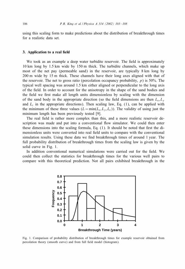
scription was made and put into a conventional 4ow simulator. We could then enterthese dimensions into the scaling formula, Eq. (1). It should be noted that !rst the di-mensionless units were converted into real !eld units to compare with the conventionalsimulation results. Using these data we !nd breakthrough times of around 1 year. Thefull probability distribution of breakthrough times from the scaling law is given by thesolid curve in Fig. 1.In addition conventional numerical simulations were carried out for the !eld. We

could then collect the statistics for breakthrough times for the various well pairs tocompare with this theoretical prediction. Not all pairs exhibited breakthrough in the

310.0

0.1

0.2

0.3

0.4

0.5

0.6

0.7

0.8

0 2 4Breakthrough Time (years)

Fre

qu

ency

Fig. 1. Comparison of probability distribution of breakthrough times for example reservoir obtained frompercolation theory (smooth curve) and from full !eld model (histogram).

P.R. King et al. / Physica A 314 (2002) 103–108 107

timescale over which the simulations were run and there were only three injectors sothere were only 9 samples. The histogram of breakthrough times is also shown in Fig. 1.Clearly with such a small sample these results cannot be taken as conclusive however,certainly they are indicative that the percolation prediction from the simple model isconsistent with the results of the numerical simulation of the more complex reservoirmodel. The agreement with the predictions is certainly good enough for engineeringpurposes. We would hope that if the simulation had been run for longer and more wellpairs had broken through that better statistics could have been collected. The mainpoint being that the scaling predictions took a fraction of a second of cpu time (andcould be carried out on a simple spreadsheet) compared with the hours required forthe conventional simulation approach. This makes this a practical tool to be used formaking engineering and management decisions.

4. Post breakthrough behaviour

So far we have only discussed the time to breakthrough. However, it is also importantto know how the oil rate declines once breakthrough has occurred. We shall studythis for only a simple system. First we consider the homogeneous case (p = 1). Ifwe consider two wells in an in!nite system then we simple need to solve Laplace’sequation (∇2p=0) with the boundary conditions that the pressure is +∞ at the injectorwell (placed at (x; y) coordinates (−r=2; 0)) and −∞ at the producer (at (r=2; 0)).Strictly speaking we should account for the !nite wellbore diameters and pressures,but this is a minor correction. Also we assume that the wells operate at constantpressure. We could also use constant rate boundary conditions but this does not alterthe essential results.We can then calculate the entire pressure !eld analytically, either by using conformal

maps or by making the simple change of variables x=r=2 sinh� =(cosh�−cos ) ; y=r=2sin =(cosh� − cos ), then pressure is associated with the coordinate � and thestreamfunction with the coordinate . This enables us to calculate the transit timealong streamline which is

tbr( ) =r2

4K[1 + (�− )cot ]

sin2

(where K is the permeability of the !eld). Asymptotically this implies that

tbr → �2r2

K(�− )3as → � :

The oil production rate is proportional to �− which implies that asymptotically theproduction rate declines like V (t) ∼ (r2=t)1=3. This is for an in!nite system. We wouldexpect this rate to decay exponentially when the streamlines see the boundaries of a!nite system.This is the case for a homogeneous reservoir. For the percolating system we expect

to see rather more complex behaviour in4uenced by the !nite boundaries or by the!nite cluster sizes away from threshold. At the percolation threshold, we expect theasymptotic decay of the oil production rate to be a power law, but with a diIerent

108 P.R. King et al. / Physica A 314 (2002) 103–108

power from the 13 found for the homogeneous case. So for p = pc we conjecture the

following asymptotic decay:

V (t → ∞) ∼(rdB

t

)�

:

Here, dB is the fractal dimension of the backbone of the percolating cluster (dB =1:6432± 0:0008 [10]). The new exponent � is found to be 0:63± 0:05 from numericalsimulations. Hence percolation theory is able to give us information, not just aboutbreakthrough times, but also post breakthrough behaviour.

5. Conclusions

We have applied results obtained earlier for the scaling law for breakthrough timedistributions for oil!eld recovery to realistic !eld data. We have shown that by makinga number of simplifying assumptions we can readily use previous results from per-colation theory to make extremely rapid estimates of the uncertainty in breakthroughtime. The agreement between the theory and the conventional simulation approach isaccurate enough for engineering purposes and therefore makes it a practical tool forsupporting decision making.

Acknowledgements

The authors thank L Gantmacher who did the calculations of postbreakthrough be-haviour for the homogeneous case. They would also like to thank J. Andrade for helpfuldiscussions and BP for !nancial support and permission to publish this paper.

References

[1] P.R. King, The use of renormalisation for calculating eIective permeability, Trans. Porous Media 4(1989) 37–58.

[2] P.R. King, A.H. Muggeridge, W.G. Price, Renormalisation calculations of immiscible 4ow, Trans.Porous Media 12 (1993) 237–260.

[3] F. Bratvedt, K. Bratvedt, C.F. Buchholz, L. Holden, H. Holden, N.H. Risebro, A new front trackingmethod for reservoir simulation, SPERE 19805, 1992.

[4] M.R. Thiele, M.J. Blunt, F.M. Orr, Modeling Flow in Heterogeneous Media using Streamtubes Part 1(299–339) & Part 2 (367–391), In Situ 19 (1995).

[5] P.R. King, The connectivity and conductivity of overlapping sandbodies, in: A.T. Buller, E. Berg,O. Hjelmeland, J. Kleppe, O. Torsaeter, J.O. Aasen (Eds.), North Sea Oil and Gas Reservoirs II,Graham & Trotman, London, 1990, pp. 353–358.

[6] S. Havlin, D. Ben-Avrahim, DiIusion in disordered media, Adv. Phys. 36 (1987) 695–798.[7] N.V. Dokholyan, Y. Lee, S.V. Buldyrev, S. Havlin, P.R. King, H.E. Stanley, Scaling of the distribution

of shortest paths in percolation, J. Stat. Phys. 93 (1998) 603–613.[8] Y. Lee, J.S. Andrade, S.V. Buldyrev, N.V. Dokholyan, S. Havlin, P.R. King, G. Paul, H.E. Stanley,

Traveling time and traveling length in critical percolation clusters, Phys. Rev. E 60 (1999) 3425–3428.[9] J.S. Andrade, S.V. Buldyrev, N.V. Dokholyan, S. Havlin, Y. Lee, P.R. King, G. Paul, H.E. Stanley,

Flow between two sites in percolation systems, Phys. Rev. E 62 (2000) 8270–8281.[10] P. Grassberger, Physica A 262 (1999) 251.