Using modal damping for full model transient analysis.Application to pantograph/catenary vibration.

J.-P. Bianchi 1, E. Balmes 1,2, G. Vermot des Roches1, A. Bobillot 3

1 SDTools44, Rue Vergniaud, 75013, Paris, Francebianchi@sdtools.com balmes@sdtools.com vermot@sdtools.com2 Arts et Metiers ParisTech, Laboratoire PIMM (SDS), CNRS UMR 8006151, boulevard de l’hopital, 75013, Paris, France3 SNCF, Direction de l’Ingenierie6, avenue Francois Mitterrand, 93574 La Plaine St Denis, Franceadrien.bobillot@sncf.fr

AbstractExperimentally, modal damping is known to allow a relatively accurate representation of damping for widefrequency ranges. For transient simulation of full finite element models, viscous damping is very often theonly formulation that is associated with an acceptable computation time. In the absence of a proper materialdamping model, it is common to assume Rayleigh damping, where the viscous matrix is a linear combinationof the mass and stiffness, or piece-wise Rayleigh damping. This representation very often results in modaldamping ratios that do not correspond to the physical reality that can be tested. One thus introduces animplicit representation of the viscous matrix that allows transient time simulation with minor time penalty,while using a much more appropriate damping representation. Modal amplitudes are also considered to post-process time simulations and analyze damping levels. When studying vibrations induced by the passage ofpantographs under a catenary, the high modal density of catenaries and the load moving over a large partof the model is a strong motivation to use full model transient analysis. Modal damping is shown to be apractical tool to analyze the properties of this complex system.

1 Introduction

Damping is the general term used to talk about physical dissipation mechanisms: material damping, friction,fluid/structure interaction, . . . Dissipation in materials is linked to viscoelasticity or other non linear consti-tutive relations. Linear viscoelasticity [1, 2, 3] is classically represented through complex moduli, which donot have time domain equivalents, or internal states, which cannot easily be incorporated in standard FEMsimulations. Friction typically occurs in joints that are either not modeled or not with sufficient detail toallow prediction.

As a result of these constraints, the physical mechanisms of damping are only modeled when such simulationis a primary objective. In other cases, one only seeks to reproduce system level behavior. In the frequencydomain, one classically specifies modal damping ratio. While in the time domain Rayleigh damping is used.The objective of this paper is to demonstrate that modal damping can efficiently and usefully be used in timedomain transient analysis.

OSCAR (Outil de Simulation du CAptage pour la Reconnaissance de defauts) is a pantograph-catenary dy-namics software developed by SNCF and SDTools and certified with respect to the EN50318 standard. Itsfirst objective is to provide signatures of defects and singularities (road bridges, turnouts, overlaps) to help

analyzing test data by extracting the relevant information. The second is to help designers to optimize exist-ing or future OCL (Overhead Contact Lines). OSCAR uses a fully 3D FEM description of OCL geometries,including stagger, tensioned beam elements for the contact wire(s) (CW) and messenger wire(s) (MW), barelements for steady arms and unilateral droppers. The pantograph can be modeled using both lumped massor multi-body models with unilateral contact law.

Computing the static shape under tension and gravity loads is a first major difficulty. Starting from designdata, that is the lengths of each component and tensions in CWs and MWs, tensions are applied first and nonlinear iterations are then used to converge on a static state. At this stage one can access to catenary elasticity,tension in each pretensioned element, static sag of the CW, modes, etc.

Pantograph description includes unilateral contact with the catenary, on one or multiple points when thereare several CWs, and possibly non linearities such as end stops, friction, active control ... Time integrationis performed using a classical implicit non linear Newmark scheme [4].

OSCAR provides the possibility of simulating the pantograph passage through a section overlap, which is avery attractive feature for assessing the different design possibilities. In this particular zone, the pantographcontacts one CW and then another, with a short period where it contacts both. One of the main issues for themodeling is then to have contact on each wire, taking into account the wire staggers.

Section 2 details the equations used for classical Rayleigh, modal and the proposed full model modal damp-ing. Modal amplitudes are then defined to be used as post-processing tools in transient analysis.

In section 3, the proposed models are used to analyze the influence of damping on catenary vibrations usinga simple pretensioned wire, an impact test on a full model and a standard pantograph passage.

2 Theory

2.1 Linear damping models

Viscous damping is a force that is proportional to velocity and leads to dynamic equations of the form

M{ ¨q(t)}+ C{ ˙q(t)}+ K{q(t)} = {f(t)} (1)

where the viscous damping matrix C is generally a symmetric semi-positive definite matrix thus ensuring apassive system.

Viscous damping is not physically representative of material damping, which is better represented by hys-teretic models where the dissipation force is proportional to displacement, or friction, which tends to onlydepend on the direction of velocity. The use of viscous damping in time domain simulations should thus beconsidered as an equivalent approach. Viscous damping is however the only dissipation mechanism that islinear and thus low cost, so that the motivation to use it in models is very strong.

The most common viscous damping description is uniform Rayleigh model, where a linear combination ofmass and stiffness matrices C = α[M ] + β[K] is used. It is typically used when one has no real knowledgeof damping: there are only two coefficients (or even one as α = 0 is often considered) to adjust to matchsome response. More elaborate approaches use a piece-wise Rayleigh damping where distinct coefficientsare used for various parts of the model

[C] =∑e

αe[Me] + βe[Ke]. (2)

The weighting αe and βe account for the fact that certain components are thought to be more dissipative thanothers and have dissipation proportional to the time derivative of displacement or deformation respectively.

Illustrations will be given in 3.2. A major limitation of this approach is that damping often occurs in junctionsthat are modeled as perfect and are thus not associated with matrices.

Real modeshapes {φj} and pulsations ωj are solutions of the eigenvalue problem

(−ω2j [M ] + [K]){φj} = {0}. (3)

When taking all modes, one has the mass orthogonality conditions and can use the fact that a matrix and itsinverse can be permuted to obtain the following relations

([Φ]T [M ])[Φ] = [Φ]T ([M ][Φ]) = I = [Φ]([Φ]T [M ]) = ([M ][Φ])[Φ]T (4)

One also has the stiffness orthogonality condition, which for mass normalized modes is given by

[Φ]T [K][Φ] =[\ω2

j \

]. (5)

Modal damping [5, 6, 7] corresponds to the assumption that the viscous damping matrix is diagonal in thereal mode basis, that is to say that

[Φ]T [C][Φ] =[\2ωjζj\

]. (6)

where ζj is the modal damping ratio of mode j. Using orthonormalization conditions (4)-(5), one can easilyshow that for uniform Rayleigh damping, one has

ζj =α

21ωj

+β

2ωj . (7)

Damping proportional to mass cannot be applied to cases with rigid body modes, since they would haveinfinite damping, and is limited to damp the first few modes since the damping decreases with frequency.Damping proportional to stiffness increases linearly with frequency which rarely corresponds to the physicalbehavior, where damping ratios are mostly constant over large frequency range.

If modal damping is a valid assumption, the Modal Strain Energy method [8] can be used and leads formodeshape {φj} to

2ζjωj =∑e

αe

(φT

j [Me]φj

)+ βe

(φT

j [Ke]φj

)(8)

In reality modes are really complex, so that the damping ratio is not associated with the real modeshape asassumed by the MSE method. As shown in [5, 7] and illustrated in figure 10, modal damping is howeveralways a good approximation for well separated modes and often a close approximation otherwise.

An important consequence of this equation is that modes where most of the energy is concentrated in elementgroup e will have a damping ratio given by αe

21ωj

+ βe

2 ωj . It also follows, as will be illustrated in figure 7, thatpiece-wise Rayleigh damping generates damping ratios that are limited by the various weighting coefficients.

In the modal basis, viscous damping is easily expressed as a diagonal matrix (6). Going back to the physicalbasis the modal diagonal matrix becomes full. Using (4), it clearly appears that [Φ]−1 = [Φ]T [M ] and[ΦT ]−1 = [M ][Φ]. One can thus invert (6) and obtain

[C] = [MΦ]N×Nm

[\2ζjωj\

]Nm×Nm

[MΦ]TNm×N (9)

The equation is exact when all modes are kept but is typically applied using a truncated modal series of Nm

modes. A key aspect of this simplification is that rows of [Φ]−1 are given by {φj}T [M ]. The C matrix in(9) is full and thus too large for practical applications. For time simulations one however needs to compute[C]{v} products, which can be organized as

[C]{v} =([MΦ]

([\2ζjωj\

] ([MΦ]T {v}

))). (10)

which involves a full transposed matrix/vector product [MΦ]T {v}, a multiplication by a diagonal matrixand a second matrix vector products. One thus only stores [MΦ] for selected modes and uses BLAS (BasicLinear Algebra Subroutines) to perform these operations. These routines are now very well parallelized andvery good performance can be achieved.

The number Nm of modes and associated damping coefficients, directly impact computation time. Part ofthe procedure is thus to select target modes that are of interest and combine with a Rayleigh model for therest of frequencies. In that case, Rayleigh damping should be compensated in order to obtain desired modaldamping ratios. For a desired ζj , one thus uses (10) with

2ζjωj = 2ζjωj − φTj C0φj (11)

where C0 is the Rayleigh damping. Compensation is exact if modal damping hypothesis (6) is verified andapproximate otherwise.

2.2 Modal amplitudes and energies

An idea closely linked with modal damping is that modal amplitudes are quantities of direct interest intransient analysis. By definition of modal coordinates, the response can be described as a linear combinationof modes

{q(t)} = [Φ]{α(t)} (12)

where {α(t)} is the vector of the modal amplitudes. Using the inverse of [Φ] implied by (4), one finds

{α(t)} = [MΦ]T {q(t)} (13)

{α(t)} = [MΦ]T {q(t)} (14)

which can easily be computed either as a post-processing step if all components of q are saved or during thetime simulation as a generalized sensor. This is a direct application of the modal sensor concept known inthe active vibration control literature.

Modal energy is the mechanical energy associated with a given mode and is given by

Emj(t) =12(αj(t)φT

j Kαj(t)φj + αj(t)φTj Mαj(t)φj) =

12(ω2

j α2j + α2

j ) (15)

In modal coordinates, mass and stiffness are diagonal matrices. It thus clearly appears that the total mechan-ical energy is the sum of modal energies.

3 Validation

This section illustrates the use of modal coordinates and damping for transient analysis of catenaries. Sec-tion 3.1 uses a simple pretensioned wire to illustrate the use of modal energies and the modal dampingproperties of Rayleigh damping. In section 3.2 an impact test is used to show how modal damping ratiocan be used to get the transient model to fit global behavior better. Finally section 3.3 illustrates how modaldamping can be used to analyze full transient analyzes.

3.1 Pretensioned wire

The example of a simple wire is first considered to illustrate the relation between transient analysis and modalquantities. The model is a tensioned wire (l=60m, T=10kN) hung every 6m to springs (K=50kN). An initial

global Raleigh with α = 0 and β = 3.25e − 3 is defined. The passage at a speed of 83m/s of a pantographwith mean contact force of 150 N is simulated.

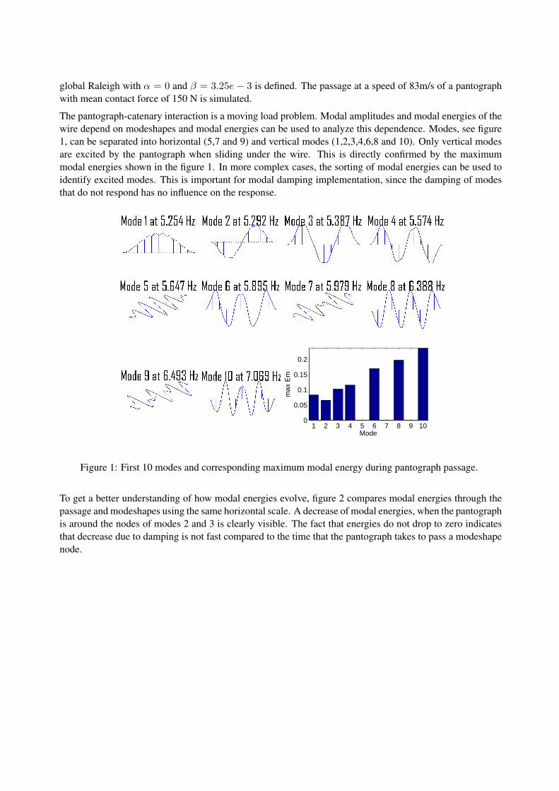
The pantograph-catenary interaction is a moving load problem. Modal amplitudes and modal energies of thewire depend on modeshapes and modal energies can be used to analyze this dependence. Modes, see figure1, can be separated into horizontal (5,7 and 9) and vertical modes (1,2,3,4,6,8 and 10). Only vertical modesare excited by the pantograph when sliding under the wire. This is directly confirmed by the maximummodal energies shown in the figure 1. In more complex cases, the sorting of modal energies can be used toidentify excited modes. This is important for modal damping implementation, since the damping of modesthat do not respond has no influence on the response.

1 2 3 4 5 6 7 8 9 100

0.05

0.1

0.15

0.2

Mode

max

Em

Figure 1: First 10 modes and corresponding maximum modal energy during pantograph passage.

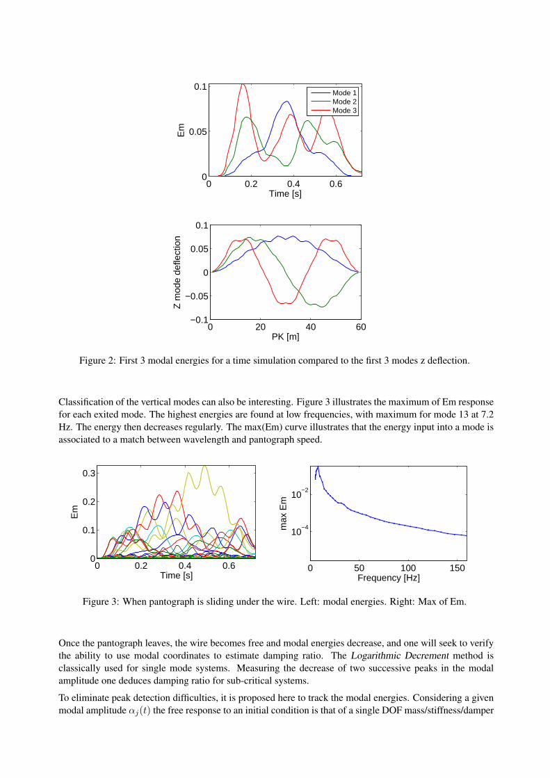
To get a better understanding of how modal energies evolve, figure 2 compares modal energies through thepassage and modeshapes using the same horizontal scale. A decrease of modal energies, when the pantographis around the nodes of modes 2 and 3 is clearly visible. The fact that energies do not drop to zero indicatesthat decrease due to damping is not fast compared to the time that the pantograph takes to pass a modeshapenode.

0 0.2 0.4 0.60

0.05

0.1

Time [s]

Em

Mode 1Mode 2Mode 3

0 20 40 60−0.1

−0.05

0

0.05

0.1

PK [m]

Z m

ode

defle

ctio

n

Figure 2: First 3 modal energies for a time simulation compared to the first 3 modes z deflection.

Classification of the vertical modes can also be interesting. Figure 3 illustrates the maximum of Em responsefor each exited mode. The highest energies are found at low frequencies, with maximum for mode 13 at 7.2Hz. The energy then decreases regularly. The max(Em) curve illustrates that the energy input into a mode isassociated to a match between wavelength and pantograph speed.

0 0.2 0.4 0.60

0.1

0.2

0.3

Time [s]

Em

0 50 100 150

10−4

10−2

Frequency [Hz]

max

Em

Figure 3: When pantograph is sliding under the wire. Left: modal energies. Right: Max of Em.

Once the pantograph leaves, the wire becomes free and modal energies decrease, and one will seek to verifythe ability to use modal coordinates to estimate damping ratio. The Logarithmic Decrement method isclassically used for single mode systems. Measuring the decrease of two successive peaks in the modalamplitude one deduces damping ratio for sub-critical systems.

To eliminate peak detection difficulties, it is proposed here to track the modal energies. Considering a givenmodal amplitude αj(t) the free response to an initial condition is that of a single DOF mass/stiffness/damper

system withm = 1, k = ω2

j , c = φTj Cφj = 2ζjωj (16)

and dynamic equationαj(t) + 2ζjωjαj(t) + ω2

j αj(t) = 0 (17)

whose characteristic equation has discriminant ∆ = 4ω2j (ζ

2j − 1).

Sub-critical damping is found for ζj < 1 (negative discriminant). There are two conjugate poles λ =ωj(−ζj ± ı

√1− ζ2

j ) and a time response of the form αj(t) = Aj cos(ωj

√1− ζ2

j t + θj) exp(−ζjωjt)where Aj and θj are two constants depending on initial conditions. Modal energy can be computed using(15) and is of the form

Emj(t) = (A + f(t)) exp(−2ζjωjt)

where f(t) << A (f is composed of sin2, cos2 and sin cos products that explains minor oscillations).

The energy decrease in a log scale plot is thus a straight line showing minor oscillations and can be estimatedwith a simple curve fit which gives an estimate of modal damping.

Critical damping is found for ζj = 1. The system then has a double pole λ = −ωj and a time response ofthe form (Aj + Bjt) exp(−ωjt) where Aj and Bj are two constants depending on initial conditions. Modalenergy is of the form Emj(t) = P (t) exp(−2γjt) where P is a second order polynomial.

Supercritical damping is found for ζj > 1. Then there are two real poles λ = ωj(−ζj ±√

ζ2j − 1) and a

time response αj(t) = (Aj exp(ωj

√ζ2j − 1t)+Bj exp(−ωj

√ζ2j − 1t)) exp(−ζjωjt) where Aj and Bj are

two constants depending on initial conditions. The exponential associated with the lowest frequency poledecreases much more slowly so that the modal energy takes the form Emj(t) ≈ (A + f(t)) exp(−2ωj(ζj −√

ζ2j − 1)t) where f is small compared to A.

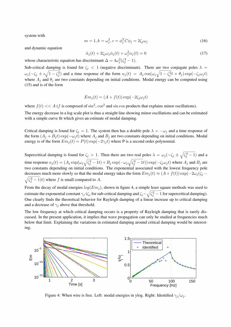
From the decay of modal energies log(Emj), shown in figure 4, a simple least square methods was used toestimate the exponential constant γj (ζj for sub-critical damping and ζj−

√ζ2j − 1 for supercritical damping).

One clearly finds the theoretical behavior for Rayleigh damping of a linear increase up to critical dampingand a decrease of γj above that threshold.

The low frequency at which critical damping occurs is a property of Rayleigh damping that is rarely dis-cussed. In the present application, it implies that wave propagation can only be studied at frequencies muchbelow that limit. Explaining the variations in estimated damping around critical damping would be interest-ing.

1 2 310

−15

10−10

10−5

Time [s]

Em

0 50 100 1500

0.5

1

1.5

Frequency [Hz]

γ j/ωj

TheoreticalIdentified

Figure 4: When wire is free. Left: modal energies in ylog. Right: Identified γj/ωj .

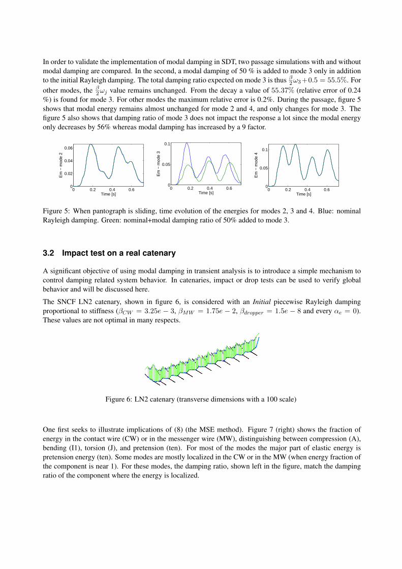
In order to validate the implementation of modal damping in SDT, two passage simulations with and withoutmodal damping are compared. In the second, a modal damping of 50 % is added to mode 3 only in additionto the initial Rayleigh damping. The total damping ratio expected on mode 3 is thus β

2 ω3+0.5 = 55.5%. Forother modes, the β

2 ωj value remains unchanged. From the decay a value of 55.37% (relative error of 0.24%) is found for mode 3. For other modes the maximum relative error is 0.2%. During the passage, figure 5shows that modal energy remains almost unchanged for mode 2 and 4, and only changes for mode 3. Thefigure 5 also shows that damping ratio of mode 3 does not impact the response a lot since the modal energyonly decreases by 56% whereas modal damping has increased by a 9 factor.

0 0.2 0.4 0.60

0.02

0.04

0.06

Time [s]

Em

− m

ode

2

0 0.2 0.4 0.60

0.05

0.1

Time [s]

Em

− m

ode

3

0 0.2 0.4 0.60

0.05

0.1

Time [s]

Em

− m

ode

4

Figure 5: When pantograph is sliding, time evolution of the energies for modes 2, 3 and 4. Blue: nominalRayleigh damping. Green: nominal+modal damping ratio of 50% added to mode 3.

3.2 Impact test on a real catenary

A significant objective of using modal damping in transient analysis is to introduce a simple mechanism tocontrol damping related system behavior. In catenaries, impact or drop tests can be used to verify globalbehavior and will be discussed here.

The SNCF LN2 catenary, shown in figure 6, is considered with an Initial piecewise Rayleigh dampingproportional to stiffness (βCW = 3.25e − 3, βMW = 1.75e − 2, βdropper = 1.5e − 8 and every αe = 0).These values are not optimal in many respects.

Figure 6: LN2 catenary (transverse dimensions with a 100 scale)

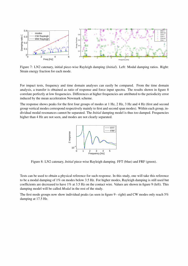
One first seeks to illustrate implications of (8) (the MSE method). Figure 7 (right) shows the fraction ofenergy in the contact wire (CW) or in the messenger wire (MW), distinguishing between compression (A),bending (I1), torsion (J), and pretension (ten). For most of the modes the major part of elastic energy ispretension energy (ten). Some modes are mostly localized in the CW or in the MW (when energy fraction ofthe component is near 1). For these modes, the damping ratio, shown left in the figure, match the dampingratio of the component where the energy is localized.

0 2 4 60

0.1

0.2

0.3

0.4

Freq [Hz]

Dam

ping

rat

io ζ

modesCW RayleighMW Rayleigh

1 2 3 4 5 6 70

0.2

0.4

0.6

0.8

1

Frequency [Hz]

Ene

rgy

Fra

ctio

n

MW AMW tenCW ACW I1CW tenCW J

Figure 7: LN2 catenary, initial piece-wise Rayleigh damping (Initial). Left: Modal damping ratios. Right:Strain energy fraction for each mode.

For impact tests, frequency and time domain analyses can easily be compared. From the time domainanalysis, a transfer is obtained as ratio of response and force input spectra. The results shown in figure 8correlate perfectly at low frequencies. Differences at higher frequencies are attributed to the periodicity errorinduced by the mean acceleration Newmark scheme.

The response shows peaks for the first four groups of modes at 1 Hz, 2 Hz, 3 Hz and 4 Hz (first and secondgroup vertical modes correspond respectively mainly to first and second span modes). Within each group, in-dividual modal resonances cannot be separated. The Initial damping model is thus too damped. Frequencieshigher than 4 Hz are not seen, and modes are not clearly separated.

0 1 2 3 4 510

−4

Frequency [Hz]

Z r

espo

nse

FFTFRF

Figure 8: LN2 catenary, Initial piece-wise Rayleigh damping. FFT (blue) and FRF (green).

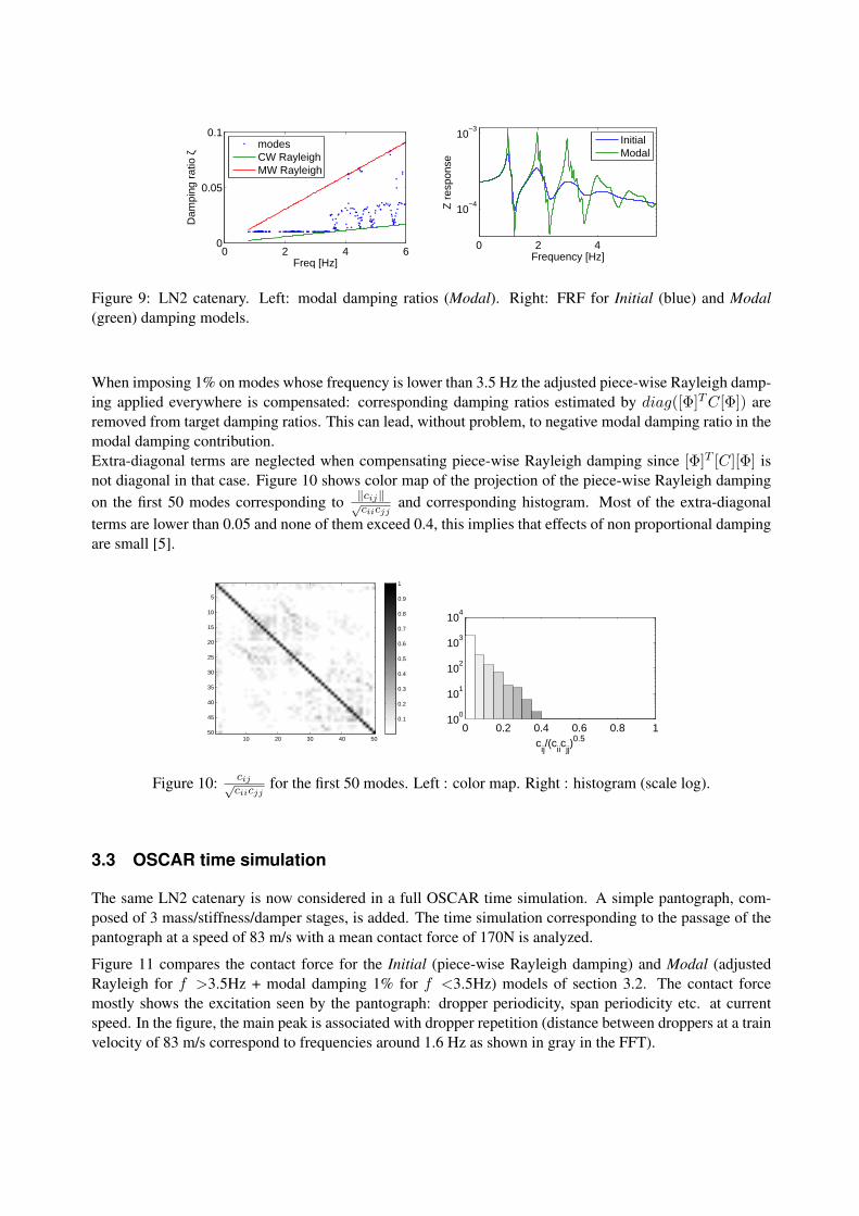
Tests can be used to obtain a physical reference for such response. In this study, one will take this referenceto be a modal damping of 1% on modes below 3.5 Hz. For higher modes, Rayleigh damping is still used butcoefficients are decreased to have 1% at 3.5 Hz on the contact wire. Values are shown in figure 9 (left). Thisdamping model will be called Modal in the rest of the study.

The first mode groups now show individual peaks (as seen in figure 9 - right) and CW modes only reach 5%damping at 17.5 Hz.

0 2 4 60

0.05

0.1

Freq [Hz]

Dam

ping

rat

io ζ

modesCW RayleighMW Rayleigh

0 2 4

10−4

10−3

Frequency [Hz]

Z r

espo

nse

InitialModal

Figure 9: LN2 catenary. Left: modal damping ratios (Modal). Right: FRF for Initial (blue) and Modal(green) damping models.

When imposing 1% on modes whose frequency is lower than 3.5 Hz the adjusted piece-wise Rayleigh damp-ing applied everywhere is compensated: corresponding damping ratios estimated by diag([Φ]T C[Φ]) areremoved from target damping ratios. This can lead, without problem, to negative modal damping ratio in themodal damping contribution.Extra-diagonal terms are neglected when compensating piece-wise Rayleigh damping since [Φ]T [C][Φ] isnot diagonal in that case. Figure 10 shows color map of the projection of the piece-wise Rayleigh dampingon the first 50 modes corresponding to ‖cij‖√

ciicjjand corresponding histogram. Most of the extra-diagonal

terms are lower than 0.05 and none of them exceed 0.4, this implies that effects of non proportional dampingare small [5].

10 20 30 40 50

5

10

15

20

25

30

35

40

45

50

0.1

0.2

0.3

0.4

0.5

0.6

0.7

0.8

0.9

1

0 0.2 0.4 0.6 0.8 110

0

101

102

103

104

cij/(c

iic

jj)0.5

Figure 10: cij√ciicjj

for the first 50 modes. Left : color map. Right : histogram (scale log).

3.3 OSCAR time simulation

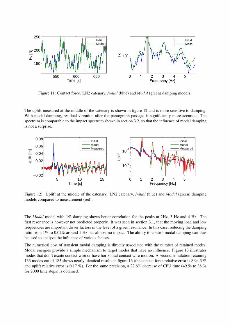
The same LN2 catenary is now considered in a full OSCAR time simulation. A simple pantograph, com-posed of 3 mass/stiffness/damper stages, is added. The time simulation corresponding to the passage of thepantograph at a speed of 83 m/s with a mean contact force of 170N is analyzed.

Figure 11 compares the contact force for the Initial (piece-wise Rayleigh damping) and Modal (adjustedRayleigh for f >3.5Hz + modal damping 1% for f <3.5Hz) models of section 3.2. The contact forcemostly shows the excitation seen by the pantograph: dropper periodicity, span periodicity etc. at currentspeed. In the figure, the main peak is associated with dropper repetition (distance between droppers at a trainvelocity of 83 m/s correspond to frequencies around 1.6 Hz as shown in gray in the FFT).

550 600 650

150

200

250

Time [s]

Fc

[N]

InitialModal

Figure 11: Contact force. LN2 catenary, Initial (blue) and Modal (green) damping models.

The uplift measured at the middle of the catenary is shown in figure 12 and is more sensitive to damping.With modal damping, residual vibration after the pantograph passage is significantly more accurate. Thespectrum is comparable to the impact spectrum shown in section 3.2, so that the influence of modal dampingis not a surprise.

5 10 15−0.02

0

0.02

0.04

0.06

0.08

Time [s]

Upl

ift [m

]

InitialModalMeasured

0 1 2 3 4 5

10−3

10−2

Frequency [Hz]

Upl

ift

InitialModalMeasured

Figure 12: Uplift at the middle of the catenary. LN2 catenary, Initial (blue) and Modal (green) dampingmodels compared to measurement (red).

The Modal model with 1% damping shows better correlation for the peaks at 2Hz, 3 Hz and 4 Hz. Thefirst resonance is however not predicted properly. It was seen in section 3.1, that the moving load and lowfrequencies are important driver factors in the level of a given resonance. In this case, reducing the dampingratio from 1% to 0.02% around 1 Hz has almost no impact. The ability to control modal damping can thusbe used to analyze the influence of various factors.

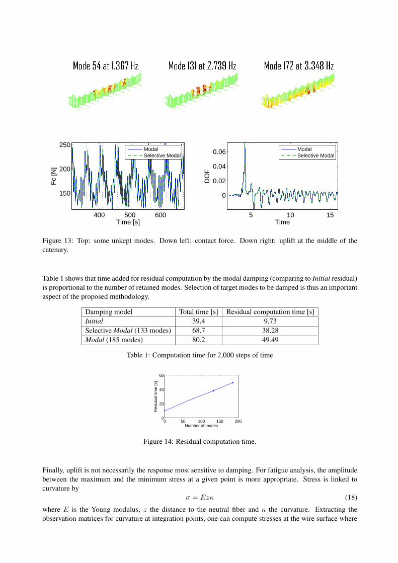
The numerical cost of transient modal damping is directly associated with the number of retained modes.Modal energies provide a simple mechanism to target modes that have no influence. Figure 13 illustratesmodes that don’t excite contact wire or have horizontal contact wire motion. A second simulation retaining133 modes out of 185 shows nearly identical results in figure 13 (the contact force relative error is 8.9e-3 %and uplift relative error is 0.17 %). For the same precision, a 22.6% decrease of CPU time (49.5s to 38.3sfor 2000 time steps) is obtained.

400 500 600

150

200

250

Time [s]

Fc

[N]

ModalSelective Modal

5 10 15

0

0.02

0.04

0.06

Time

DO

F

ModalSelective Modal

Figure 13: Top: some unkept modes. Down left: contact force. Down right: uplift at the middle of thecatenary.

Table 1 shows that time added for residual computation by the modal damping (comparing to Initial residual)is proportional to the number of retained modes. Selection of target modes to be damped is thus an importantaspect of the proposed methodology.

Damping model Total time [s] Residual computation time [s]Initial 39.4 9.73Selective Modal (133 modes) 68.7 38.28Modal (185 modes) 80.2 49.49

Table 1: Computation time for 2,000 steps of time

0 50 100 150 2000

20

40

60

Number of modes

Res

idua

l tim

e [s

]

Figure 14: Residual computation time.

Finally, uplift is not necessarily the response most sensitive to damping. For fatigue analysis, the amplitudebetween the maximum and the minimum stress at a given point is more appropriate. Stress is linked tocurvature by

σ = Ezκ (18)

where E is the Young modulus, z the distance to the neutral fiber and κ the curvature. Extracting theobservation matrices for curvature at integration points, one can compute stresses at the wire surface where

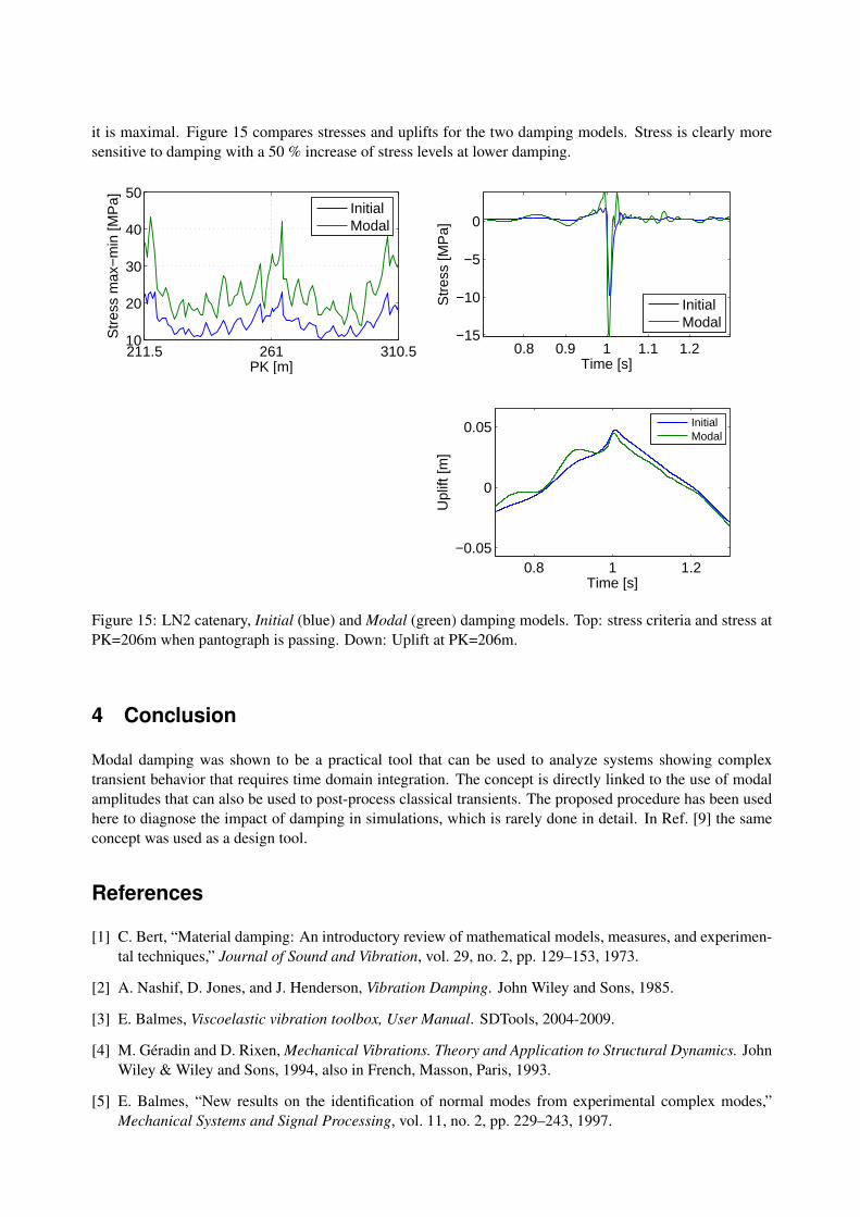
it is maximal. Figure 15 compares stresses and uplifts for the two damping models. Stress is clearly moresensitive to damping with a 50 % increase of stress levels at lower damping.

211.5 261 310.510

20

30

40

50

PK [m]

Str

ess

max

−m

in [M

Pa]

InitialModal

0.8 0.9 1 1.1 1.2−15

−10

−5

0

Time [s]

Str

ess

[MP

a]

InitialModal

0.8 1 1.2−0.05

0

0.05

Time [s]

Upl

ift [m

]

InitialModal

Figure 15: LN2 catenary, Initial (blue) and Modal (green) damping models. Top: stress criteria and stress atPK=206m when pantograph is passing. Down: Uplift at PK=206m.

4 Conclusion

Modal damping was shown to be a practical tool that can be used to analyze systems showing complextransient behavior that requires time domain integration. The concept is directly linked to the use of modalamplitudes that can also be used to post-process classical transients. The proposed procedure has been usedhere to diagnose the impact of damping in simulations, which is rarely done in detail. In Ref. [9] the sameconcept was used as a design tool.

References

[1] C. Bert, “Material damping: An introductory review of mathematical models, measures, and experimen-tal techniques,” Journal of Sound and Vibration, vol. 29, no. 2, pp. 129–153, 1973.

[2] A. Nashif, D. Jones, and J. Henderson, Vibration Damping. John Wiley and Sons, 1985.

[3] E. Balmes, Viscoelastic vibration toolbox, User Manual. SDTools, 2004-2009.

[4] M. Geradin and D. Rixen, Mechanical Vibrations. Theory and Application to Structural Dynamics. JohnWiley & Wiley and Sons, 1994, also in French, Masson, Paris, 1993.

[5] E. Balmes, “New results on the identification of normal modes from experimental complex modes,”Mechanical Systems and Signal Processing, vol. 11, no. 2, pp. 229–243, 1997.

[6] T. Caughey, “Classical normal modes in damped linear dynamic systems,” ASME J. of Applied Mechan-ics, pp. 269–271, 1960.

[7] T. Hasselman, “Modal coupling in lightly damped structures,” AIAA Journal, vol. 14, no. 11, pp. 1627–1628, 1976.

[8] L. Rogers, C. Johson, and D. Keinholz, “The modal strain energy finite element method and its applica-tion to damped laminated beams,” Shock and Vibration Bulletin, vol. 51, 1981.

[9] G. Vermot des Roches, E. Balmes, R. Lemaire, and T. Pasquet, “Designed oriented time/frequencyanalysis of contact friction instabilities in application to automotive brake squeal,” in Vibrations, Chocs& Bruit (VCB XVIIth symposium), 2010.