using mathematica to study complex numbers (week...

Using Mathematica to study complex numbers (week 3)

ü BasicsMathematica is set up to deal with complex numbers, although there are some tricks one has to learn. The simplestway to enter i (square root of -1) is as I (upper case I).z = 2 + 3 I

2 + 3 Â

Note that Mathematica writes I in lowercase in the output. Here's another example:Sqrt@-4D

2 Â

Real & Imaginary parts, Magnitude (=absolute value) & Argument, and Complex Conjugate are obtained as follows:Re@zD

2

Im@zD

3

Abs@zD

13

Arg@zD

ArcTanB3

2F

N@Arg@zDD

0.982794

zbar = Conjugate@zD

2 - 3 Â

Complex numbers can be added, subtracted, multiplied and divided as for reals:z + zbar

4

(which is correct as the sum should be twice the real part of z)z - zbar

6 Â

(again correct as the sum gives twice the imaginary part of z times I)z zbar

13

(which is correct since it is the square of the magnitude of z)z ê zbar

-5

13+12 Â

13

8Abs@z ê zbarD, N@Arg@z ê zbarDD<

81, 1.96559<

(which is correct since, as seen in lectures, z/zbar has magnitude 1 and argument twice that of z)

Note that Mathematica’s convention for the argument is -p < Arg[z] § p8Arg@1D, Arg@ID, Arg@-1D, Arg@-ID<

:0,p

2, p, -

p

2>

Also, by convention, Arg[0]=0Arg@0D

0

ü Simple examples of manipulating complex numbersExample discussed previously in class: Result is displayed automatically in “x + i y” form.z2 = H3 + IL ê H2 + IL

7

5-

Â

5

To get result in polar form:8r = Abs@z2D, theta = Arg@z2D<

: 2 , -ArcTanB1

7F>

One can also enter the complex number in polar form---all Mathematica functions take complex arguments.z2polar = r Exp@I thetaD

2 ‰-Â ArcTanB

1

7F

To get back in Cartesian form use the useful function "ComplexExpand"ComplexExpand@z2polarD

7

5-

Â

5

Another example from previous lectures:z3 = H5 - 2 IL ê H5 + 2 IL

21

29-20 Â

298Abs@z3D, Arg@z3D<

:1, -ArcTanB20

21F>

A final exampleAbs@H2 + 3 IL ê H1 - ILD

13

2

2 ComplexAdditions.nb

ü Features of ComplexExpandMathematica usually assumes that numbers are complex. Thus inz4 = Hx + I yL^2

Hx + Â yL2

it assumes that x and y are complex:8Re@z4D, Im@z4D<

9ReAHx + Â yL2E, ImAHx + Â yL2E=

One nice feature of ComplexExpand is that it assumes that all variables are real (unless you tell it otherwise). ComplexExpand@Hx + I yL^2D

x2 + 2 Â x y - y2

ü RootsMathematica does not automatically give all complex roots, e.g.H1L^81 ê 3<

81<

To get all the roots we can use Solve. (Note that we have to "Clear" z, since it was defined above.)Clear@zD; Solve@z^3 ã 1, zD

98z Ø 1<, 9z Ø -H-1L1ê3=, 9z Ø H-1L2ê3==

To get the result in “x+iy” form use ComplexExpand:root = ComplexExpand@Solve@z^3 ã 1, zDD

:8z Ø 1<, :z Ø -1

2-

Â 3

2>, :z Ø -

1

2+

Â 3

2>>

Note that Mathematica gives the results as a list of assignments (which I have labeled "root"). We can use this list withthe following construction involving "/."(Read this as "Evaluate z with the assignment rules in root, one at a time".)z ê. root

:1, -1

2-

Â 3

2, -

1

2+

Â 3

2>

In this way we can check that all 3 roots are really roots:ComplexExpand@z^3 ê. rootD

81, 1, 1<

Here is one way to plot the roots

ComplexAdditions.nb 3

rootplot = ListPlot@8Re@zD, Im@zD< ê. root, PlotRange Ø 88-1.1, 1.1<, 8-1.1, 1.1<<,AxesLabel Ø 8"ReHzL", "ImHzL"<, AspectRatio Ø 1, PlotStyle -> [email protected]

-1.0 -0.5 0.5 1.0ReHzL

-1.0

-0.5

0.5

1.0

ImHzL

Showing that the roots lie on the "unit circle"Show@rootplot, Graphics@8Red, Circle@80, 0<, 1D<DD

-1.0 -0.5 0.5 1.0ReHzL

-1.0

-0.5

0.5

1.0

ImHzL

Here is a plot of the fifth roots of -32 (which includes -2). Note the use of "Module" to package all the commands intoone unit. The initial parenthesis "{root,rootplot}" lists the local names that are used---these do not get defined outsideof the Module, and thus do not overwrite other values.


Module@8root, rootplot<, root = Solve@z^5 ã -32, zD;rootplot = ListPlot@8Re@zD, Im@zD< ê. root, PlotRange Ø 88-2.1, 2.1<, 8-2.1, 2.1<<,

AxesLabel Ø 8"ReHzL", "ImHzL"<, AspectRatio Ø 1, PlotStyle -> [email protected];Show@rootplot, Graphics@8Red, Circle@80, 0<, 2D<DDD

-2 -1 1 2ReHzL

-2

-1

1

2

ImHzL

ü Complex SeriesEverything that works for real series in Mathematica (and which we discussed before) was actually working all alongfor complex seriesSum1@z_D = Sum@z^n ê Sqrt@nD, 8n, 1, Infinity<D

PolyLogB1

2, zF

The disk of convergence has radius 1 for this sum. On the boundary, the sum diverges at some point and converges atothers:Sum1@1D

ComplexInfinity

N@Sum1@IDD

-0.427728 + 0.667691 Â

N@Sum1@-1DD

-0.604899

Mathematica infact knows how to "analytically continue" the function outside of its disk of convergence (somethingwe may discuss later), e.g.N@Sum1@1 + IDD

-0.482402 + 1.43205 Â

ü Complex FunctionsHere are some basic examples: everything works for complex arguments.


N@Sin@1 + 2 IDD

3.16578+ 1.9596 Â

ComplexExpand@Sin@x + I yDD

Cosh@yD Sin@xD + Â Cos@xD Sinh@yD

For Logs and powers Mathematica makes standard choices to resolve the ambiguity in the argument of the logarithm.Note that the N[] (for numerically evaluate) is need to get an actual numerical result. Note that //N after a commandhas the same effect.Log@3 + ID

Log@3 + ÂD

N@Log@3 + IDD

1.15129+ 0.321751 Â

Log@3 + ID êê N

1.15129 + 0.321751 Â

H1 + 2 IL^H3 + IL

H1 + 2 ÂL3+Â

N@H1 + 2 IL^H3 + ILD

-2.0442 - 3.07815 Â

ü Plotting Complex FunctionsComplex valued function can be difficult to visualize due to depending on multiple variables and functions behavingdifferently along the imaginary axis. Using Mathematica’s 2D plots separately for the real and imaginary parts,contour plots and 3D plots can greatly help. The following are a few examples.Looking at the exponential function ez for a purely imaginary argumentPlot@8Re@Exp@I * xDD, Im@Exp@I * xDD, Abs@Exp@I * xDD<,8x, -10, 10<, PlotStyle Ø 88Thick, Blue<, 8Thick, Red<, 8Thick, Green<<D

-10 -5 5 10

-1.0

-0.5

0.5

1.0

We can see the real part (blue) is a Cos[] whereas the imaginary part (red) is a Sin[] and the magnitude stays a constantvalue of 1.Here is a contour plot with a general complex argument.


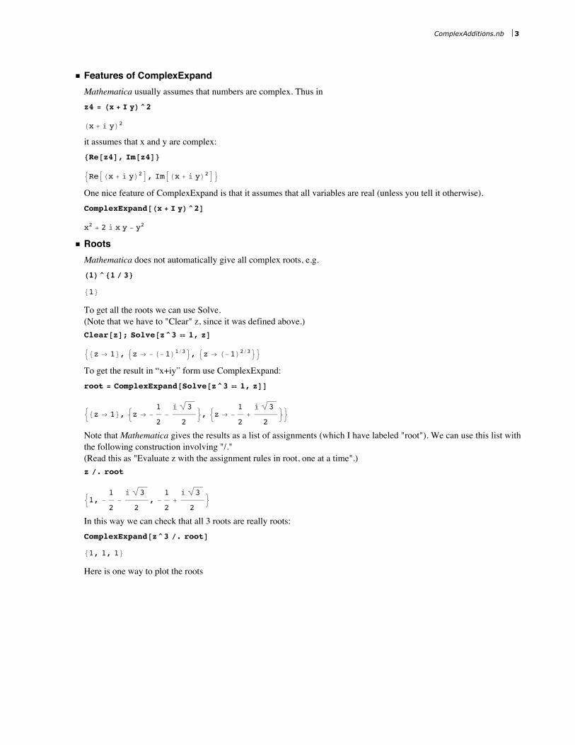
ContourPlot@Re@Exp@x + I * yDD, 8x, -10, 10<, 8y, -10, 10<,Contours Ø 20, ContourShading Ø Automatic, ColorFunction Ø "Rainbow"D

The more red the the region is, the larger the function is, the more blue, the smaller.

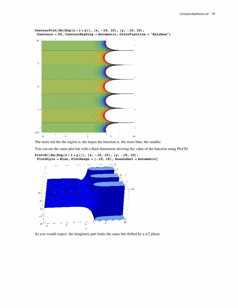
You can see the same plot but with a third dimension showing the value of the function using Plot3DPlot3D@8Re@Exp@x + I * yDD<, 8x, -10, 10<, 8y, -10, 10<,PlotStyle Ø Blue, PlotRange Ø 8-10, 10<, AxesLabel Ø AutomaticD

As you would expect, the imaginary part looks the same but shifted by a p/2 phase


Plot3D@8Im@Exp@x + I * yDD<, 8x, -10, 10<, 8y, -10, 10<,PlotStyle Ø Red, PlotRange Ø 8-10, 10<, AxesLabel Ø AutomaticD

Here they are together.Plot3D@8Re@Exp@x + I * yDD, Im@Exp@x + I * yDD<, 8x, -10, 10<, 8y, -10, 10<,PlotStyle Ø 8Blue, Red<, PlotRange Ø 8-10, 10<, AxesLabel Ø AutomaticD

These sorts of plots can be especially useful for visualizing branch cuts, such as the one along the negative real line forthe Log[ ] function.Please note that Mathematica chooses to put the discontinuity in the imaginary part of the Logarithm between -p and+p, rather than between 0 and 2p, as discussed in class. This moves the “branch cut” to the negative real axis.


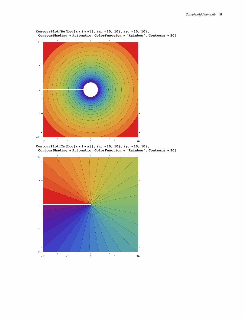
ContourPlot@Re@Log@x + I * yDD, 8x, -10, 10<, 8y, -10, 10<,ContourShading Ø Automatic, ColorFunction Ø "Rainbow", Contours Ø 20D

ContourPlot@Im@Log@x + I * yDD, 8x, -10, 10<, 8y, -10, 10<,ContourShading Ø Automatic, ColorFunction Ø "Rainbow", Contours Ø 30D


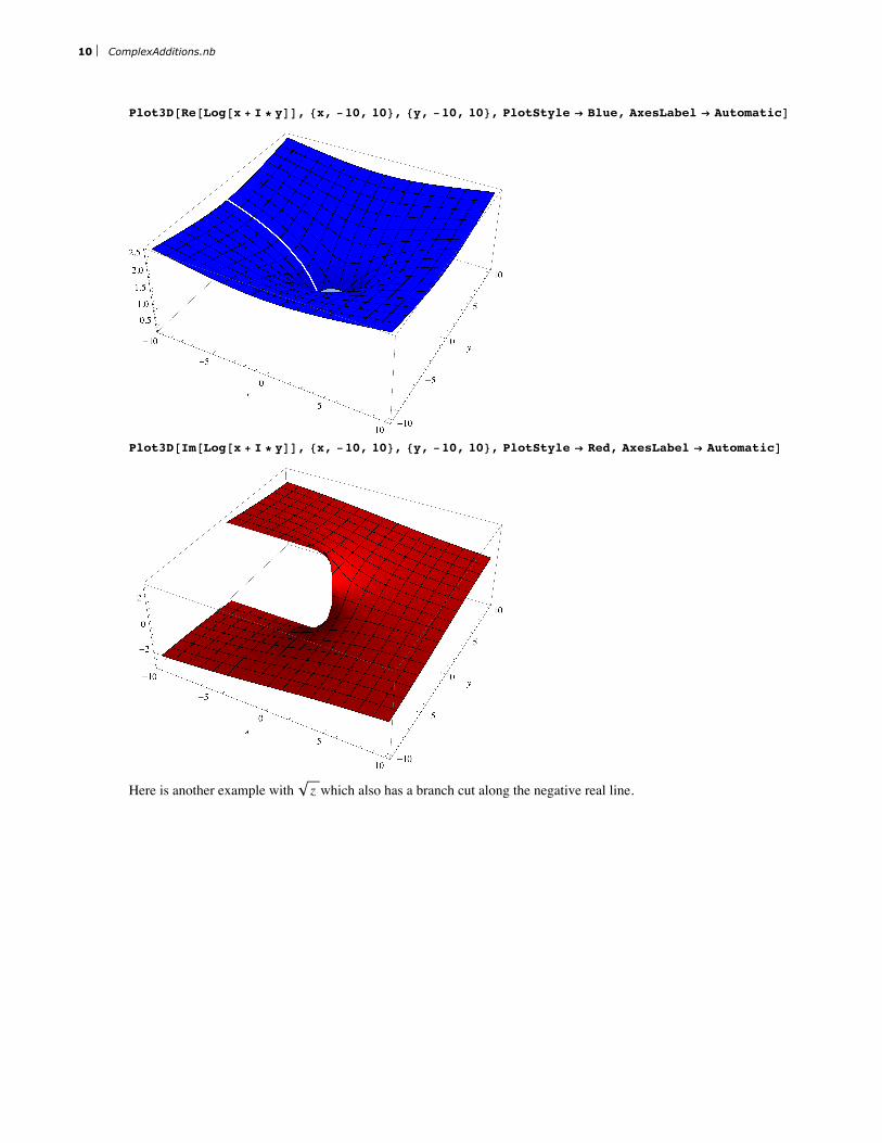
Plot3D@Re@Log@x + I * yDD, 8x, -10, 10<, 8y, -10, 10<, PlotStyle Ø Blue, AxesLabel Ø AutomaticD

Plot3D@Im@Log@x + I * yDD, 8x, -10, 10<, 8y, -10, 10<, PlotStyle Ø Red, AxesLabel Ø AutomaticD

Here is another example with z which also has a branch cut along the negative real line.


ContourPlotBReB x + I * y F, 8x, -10, 10<, 8y, -10, 10<, AxesLabel Ø Automatic,

ContourShading Ø Automatic, ColorFunction Ø "Rainbow", Contours Ø 20F

ContourPlotBImB x + I * y F, 8x, -10, 10<, 8y, -10, 10<, AxesLabel Ø Automatic,

ContourShading Ø Automatic, ColorFunction Ø "Rainbow", Contours Ø 20F


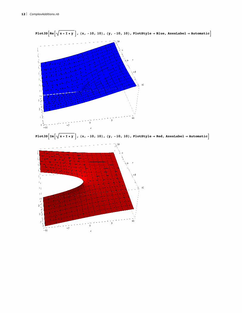
Plot3DBReB x + I * y F, 8x, -10, 10<, 8y, -10, 10<, PlotStyle Ø Blue, AxesLabel Ø AutomaticF

Plot3DBImB x + I * y F, 8x, -10, 10<, 8y, -10, 10<, PlotStyle Ø Red, AxesLabel Ø AutomaticF


using mathematica to study complex numbers (week...

Documents