using flow geometry for drifter deployment in … flow geometry for drifter deployment in ... the...

Tellus 000, 000–000 (0000) Printed 26 April 2007 (Tellus LATEX style file v2.2)

Using Flow Geometry for Drifter Deployment in

Lagrangian Data Assimilation

By H. Salman1⋆, K. Ide2 and C. K. R. T. Jones1,1Department of Mathematics, University of North Carolina at Chapel Hill, Chapel Hill, North Carolina, USA;

2Department of Atmospheric and Oceanic Sciences & Institute of Geophysics and Planetary Physics, University of California,

Los Angeles, California, USA

(Manuscript received ???; in final form ???)

ABSTRACTMethods of Lagrangian data assimilation (LaDA) require carefully chosen sites for op-timal drifter deployments. In this work, we investigate a directed drifter deploymentstrategy with a recently developed LaDA method employing an augmented state vec-tor formulation for an Ensemble Kalman filter. We test our directed drifter deploymentstrategy by targeting Lagrangian coherent flow structures of an unsteady double gyreflow to analyze how different release sites influence the performance of the method.We consider four different launch methods; a uniform launch, a saddle launch in whichhyperbolic trajectories are targeted, a vortex center launch, and a mixed launch tar-geting both saddles and centers. We show that global errors in the flow field requiregood dispersion of the drifters which can be realized with the saddle launch. Localerrors on the other hand are effectively reduced by targeting specific flow features.In general, we conclude that it is best to target the strongest hyperbolic trajectoriesfor shorter forecasts although vortex centers can produce good drifter dispersion uponbifurcating on longer time-scales.

1 Introduction

Increasing interest in Lagrangian data has led to recentdevelopments in using such data for improving predictions ofthe ocean (Carter, 1989; Kamachi and O’Brien, 1995; Mol-card et al., 2003; Ozgokmen et al., 2003). These methods relyon reconstructing Eulerian velocity information from consec-utive measurements of drifter positions which are then as-similated into Eulerian flow models. An alternative method,developed by Kuznetsov et al. (2003) and Ide et al. (2002),which employs an augmented state vector formulation to-gether with an Extended Kalman Filter, has been shownto maximize the information content in comparison to theabove approaches for Lagrangian data assimilation (LaDA).In stark contrast to the aforementioned methods, the aug-mented state vector formulation allows one to evolve theerror correlations between the Eulerian flow variables anddrifter coordinates in a way that is entirely consistent withthe evolution of error correlations in Eulerian data assimi-lation. The method of Kuznetsov et al. (2003) and Ide et al.(2002), therefore, bypasses the need to introduce approxi-mations in the reconstruction of Eulerian velocity informa-tion. The augmented state vector formulation has recentlybeen applied, together with an Ensemble Kalman filter, toa shallow water model of the ocean by Salman et al. (2006).

⋆ Corresponding author.

Current address: Department of Applied Mathematics and The-oretical Physics, Centre for Mathematical Sciences, University ofCambridge, CB3 0WA, UK; E-mail: [email protected]

The work of Salman et al. clearly illustrated the success ofthe method by establishing that the filter is stable providedthat data is assimilated more frequently than the Lagrangianautocorrelation time-scale (TL). Methods that reconstructEulerian velocity information, on the other hand, report amaximum allowable time-interval of 0.2TL. The augmentedstate vector formulation is, therefore, indispensable in sce-narios where infrequent measurements are available.

Salman et al. (2006) carefully analyzed the performanceof the method with respect to variations in different param-eters, including the number of ensembles, the localizationof the covariance matrix, and the drifter release sites. Ofthese parameters, the most difficult to understand, and yetperhaps most important, is the initial launch sites of thedrifters. The root of the difficulty is two-fold; firstly it hasbeen known for sometime now that simple unsteady two-dimensional velocity fields can give rise to chaotic advectionin the motion of Lagrangian material particles (Aref, 1984;Aref and El Naschie, 1994). Such chaotic behavior has cometo be known as Lagrangian chaos and reflects a degree of un-predictability in the motion of material particles. Given thata good first order approximation that describes the motionof floats and drifters is to assume that they behave as mate-rial particles (Bower, 1991), understanding their motion inunsteady flows is extremely nontrivial. In light of these re-sults, understanding how drifter release locations affect theperformance of our LaDA requires a more in depth under-standing of what controls the trajectories of these drifters.The above difficulty is compounded by a second nonlineareffect in that the velocity field that governs the motion of the

c© 0000 Tellus

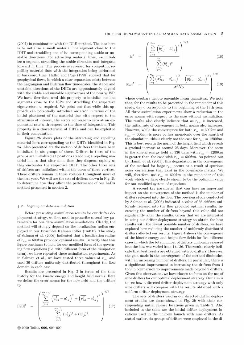
2 H. SALMAN ET AL.

drifters is part of the state vector that is being updated byour assimilation algorithm. This sets in a two-way couplingbetween the positions of the drifters and the their impacton the method. With such complications, the preliminaryresults presented in Salman et al. (2006) regarding the in-fluence of different release sites on the performance of themethod are not fully conclusive.

In this study, we aim to provide a more in depth and di-rect understanding of how different initial drifter placementscan affect the performance of the LaDA method presented inSalman et al. (2006). Our approach will be to employ recentideas from dynamical systems theory (Jones and Winkler,2002) to extract Lagrangian coherent structures (LCS) fromour numerically computed flows. These Lagrangian struc-tures have been studied extensively for geophysical flows inrecent years and are understood to orchestrate the evolutionand motion of material particles (see Wiggins (2005) for arecent review). They provide a geometric approach to ana-lyze the motion of particles in unsteady 2D velocity fields.By extracting such structures from our flow, the complica-tions that arise from the nonlinear dependence of the drifterpositions on the underlying advecting flow field reduce tounderstanding the evolution of a set of material lines thatdelineate such flow structures.

While this approach has proven to be successful in anumber of studies conducted to date (Coulliette and Wig-gins, 2000; Poje and Haller, 1999; Jones and Winkler, 2002;Kuznetsov et al., 2002; Mancho et al., 2004), we are posedwith an additional difficulty here due to the two-way cou-pling between the drifter positions and the velocity fieldthat arises from assimilation. To simplify the problem inthis study, we will focus on a twin-experiment configurationin which the flow field for the synthetic “truth” is known.Under such idealized conditions, we can extract the LCSfor the true state and use this as our template for the di-rected launch of drifters. The approach we will adopt will,therefore, build on the ideas used by Poje et al. (2002), andToner and Poje (2004) to study how initial drifter place-ments influences the performance of our LaDA method. Bytargeting the Lagrangian flow structures of the “true” sys-tem, we are able to simplify the problem drastically. At thesame time, it enables us to focus on the structures of mostrelevance since it is these structures that control the motionof the drifter positions being assimilated into the model.This simplification also serves as a relevant benchmark casefor future studies geared towards the design of an observingsystem for the optimal deployment of drifters for use withour LaDA formulation. In such a case, one is interested inwhere to release drifters to improve ocean forecasting with-out prior knowledge of the “true” state of the system. Thedesign of such a system introduces major challenges and it,therefore, helps to understand how the flow structures af-fect our data assimilation method under the more idealizedscenario of a twin-experiment setup. This in turn would al-low us to determine how much improvement we can expectto gain from directed drifter placement in relation to ran-dom drifter placement before embarking on the involved de-sign of such an observing system. A similar approach hasbeen adopted in the study of Molcard et al. (2006) who an-alyzed how directed drifter deployment affected the conver-gence of the data assimilation method developed by Molcardet al. (2003), and Ozgokmen et al. (2003). As stated earlier,

however, the formulation of our LaDA scheme is fundamen-tally different from these methods. The work presented here,therefore, provides an essential first step towards the devel-opment of a Lagrangian observing system for the methodsdeveloped by Ide et al. (2002), Kuznetsov et al. (2003), andSalman et al. (2006).

The remainder of the paper is organized into four mainsections. We begin in section 2 by stating the main elementsof our LaDA method that is based on the use of the En-semble Kalman filter. The mathematical model used in thisstudy together with the problem setup is briefly describedin section 3. We then describe how we compute the LCSfor our double gyre flow and present results using two dif-ferent methods. The first method computes relative disper-sion, produced by integrating material particles in forwardand backward time, to locate regions of maximal stretch-ing within the flow. The second method employs the idea ofstraddling one of the stable or unstable directions of a dis-tinguished hyperbolic trajectory (DHT) to compute the La-grangian structures of interest. These Lagrangian templatesare used to identify different release sites for sets of driftersthat consequently have very different dispersion character-istics. Results are subsequently presented in section 4 toquantify how targeting specific regions of the flow can af-fect our data assimilation method. We end in section 5 withconclusions of the main results.

2 Ensemble Kalman filter for Lagrangian data

In this section, we will summarize the key elementsof the formulation developed by Salman et al. (2006),Kuznetsov et al. (2003), and Ide et al. (2002) for assimi-lating Lagrangian data. We begin by writing our system ofequations governing the (NF × 1) flow state vector, xF , andthe (2ND × 1) drifter state vector, xD, of our ND drifters interms of the augmented state vector, x = (xT

F ,xTD)T . Using

an ensemble forecast with NE members, we have

dxfj

dt= mj(xj , t), j = 1, · · · , NE . (1)

Here, the subscript j denotes the ensemble member, the su-perscript f denotes the system forecast, and mj is the evo-lution operator. Using this augmented system of equationsfor each member of the ensemble, we can define the corre-sponding covariance matrix by

Pf =

1

NE − 1

NE∑

j=1

(xfj − xf )(xf

j − xf )T . (2)

We note that the covariance matrix can be expressed inblock matrix form as

Pf =

(P

fFF P

fFD

PfDF P

fDD

). (3)

PFF , PFD, PDF , and PDD are (NF × NF ), (NF × 2ND),(2ND ×NF ), and (2ND ×2ND) matrices, respectively. Theycorrespond to correlations between the flow and drifter partsof the state vector. The mean of the state vector taken overthe ensemble is denoted by an over-line in Eq. (2) and is

c© 0000 Tellus, 000, 000–000

DRIFTER DEPLOYMENT IN LAGRANGIAN DATA ASSIMILATION 3

defined as

xf =1

NE

NE∑

j=1

xfj . (4)

When Lagrangian measurements become available, the anal-ysis state of the system, denoted by xa, can be obtainedusing the perturbed observation Ensemble Kalman filter(Evensen, 1994; 2003). The filter updates each ensemblemember by

xaj = x

fj + Kdj , (5)

where the Kalman gain matrix is defined as

K =

(ρFD PFD

ρDD PDD

)(ρDD PDD + R)−1 , (6)

and the innovation vector dj is given by

dj = yo − Kx

fD,j + ǫ

fj . (7)

The observation vector yo represents noisy spatial coordi-nates of the drifters in the zonal and meridional directions.Both the noise in the drifters’ positions and the perturba-

tions to the observations given by ǫfj are drawn from a gaus-

sian distribution with a covariance matrix equal to R. The

latter is also made to satisfy the condition 1/NE

∑NE

j=1ǫ

fj =

0.In Eq. (6), the operator denotes the Schur product

between two matrices. The elements of the matrix ρ cor-respond to a distance-dependent correlation function . Wehave used the correlation function given by Gaspari andCohn (1999) which is smooth and has compact support.

3 Flow model and experimental setup

The model we employ in this study is very similar to theone used in the work of Salman et al. (2006). The model is anidealized ocean model with a square domain configurationwhose size in the zonal and meridional directions are denotedby Lx and Ly, respectively. As described in Cushman (1994)and Pedlosky (1986), the flow within this domain can bemodeled by the reduced gravity shallow water system ofequations which are given by

∂h

∂t= −

∂(hu)

∂x−

∂(hv)

∂y, (8)

∂u

∂t= −u · ∇u + fv − g′ ∂h

∂x+ F u +

1

h

(∂τxx

∂x+

∂τxy

∂y

),

∂v

∂t= −u · ∇v − fu − g′ ∂h

∂y+

1

h

(∂τyx

∂x+

∂τyy

∂y

). (9)

h is the surface height, (u, v) is the fluid-velocity vector, g′ isthe reduced gravity, F u is a horizontal wind-forcing actingin the zonal direction, and f is the Coriolis parameter. Weinvoke the β-plane approximation allowing the Coriolis termto be expressed as

f = fo + βy, (10)

where fo and β are constants. A zonal wind-forcing of theform

F u =−τo

ρHo(t)cos (2πy/Ly), (11)

Ho(t) =1

LxLy

∫ Lx

0

∫ Ly

0

h(x, y, t)dxdy, (12)

is employed in this work where x and y are the coordinatesin the zonal and meridional directions measured from thewestern and southern boundaries of our flow domain, re-spectively, τo is the wind stress, ρ is the density of water,and Ho(t) is the average water depth.

In contrast to the study presented in Salman et al.(2006), we have replaced the dissipation term by the formproposed by Schar and Smith (1993). This is given by

τij = νh

(∂ui

∂xj+

∂uj

∂xi− δij

∂uk

∂xk

), (13)

for all possible permutations of the indices i and j, whichcan take the two cartesian components x or y, and ν de-notes a (constant) eddy viscosity of the flow. This formof the dissipation term has been employed as it leads toa self-consistent formulation of the shallow-water system ofequations as further discussed by Shchepetkin and O’Brien(1996), and Gent (1993). In particular, the resulting equa-tions satisfy energy and momentum conservation principlesthat are otherwise violated with the form of the dissipationemployed in Salman et al. (2006).

The above equations are supplemented with the bound-ary and initial conditions given by

u(x, y, t)|∂Ω = 0, v(x, y, t)|∂Ω = 0, (14)

u(x, y, 0) = 0, v(x, y, 0) = 0, h(x, y, 0) = Ho, (15)

where ∂Ω represents the boundaries of our flow domain. Tosetup a double gyre circulation, we solved the above equa-tions with the model parameters given in Table 1.

Equations (8-9) were discretized on a uniform meshwith (nx ×ny) = (100× 100) grid points which correspondsto a grid spacing of (∆x×∆y) = (20km× 20km). This pro-duces a set of NF = 2(nx − 1)(ny − 1) + nxny equationsfor the flow which correspond to the flow state vector xF .In addition, a set of 2ND equations corresponding to thezonal and meridional coordinates of the ND drifters was in-tegrated together with the flow. The drifters were assumedto be advected as material particles by the flow field. Atwin-experiment setup was used for our assimilation exper-iments. The synthetic truth (control run) was obtained byintegrating the model for 12 years from an initial flow atrest using an average water depth of Ho = 500m. The flowfor the forecast was made up of an ensemble consisting of80 members. The ensemble was generated by perturbing theinitial height field of each member so that the mean waterdepth taken over the ensemble is given by Ho = 550m. Agaussian distribution with a variance of σh = 50m was usedto generate Ho for the different members of the ensemble.Each member was then integrated forward in time for a 12year period to produce a set of flows corresponding to thedifferent initial height fields. At the beginning of the 13thyear, drifters were released into the true flow. Each drifterwas initialized at a specified location within the flow domainand then integrated with our true flow over a period of twoyears to generate a set of true trajectories. The observationerrors corresponding to these drifter trajectories were takento be distributed as independent gaussians with the same

c© 0000 Tellus, 000, 000–000

4 H. SALMAN ET AL.

statistics; that is

E[ǫ(tk)ǫT (tl)] = δklσ2I, (16)

E[ǫ(tk)] = E[ǫ(tk)] = 0.

where σ was taken to be 200m in this work. Each ensemblemember of our forecast model was then integrated over thesame two year time interval using a corresponding set ofperturbed drifters with the same error statistics as thosegiven in Eq. (16).

When performing our assimilation experiments, we havefixed the assimilation time interval to be equal to 1 day. Thisis well within the Lagrangian autocorrelation time-scale of10 days for this flow (Salman et al., 2006). Consequently, wewill avoid the potential problems of filter divergence thatcan arise with the use of larger time intervals.

4 Results

4.1 Computation of Lagrangian coherent structures

In this work, we will employ our knowledge of the ‘true’velocity field to extract the desired LCS that control themotion of the observed drifter positions. The computationof LCS from a numerically computed velocity field with gen-eral time dependence is a topic that has received much at-tention in recent years (Wiggins, 2005). In general, the firststep with any such method is to locate distinguished hy-perbolic trajectories (DHTs) associated with the flow givenover some finite time interval [t0, t1]. For time-periodic flows,such points can easily be identified as the fixed points of anappropriately chosen Poincare map of the flow. However, forflows with general time-dependence, the DHTs are aperiodicin time. Identifying them, therefore, requires the use of alter-native methods that have found varying degrees of success indifferent applications. The first approach is based on the ideathat for flows having a Lagrangian time-scale much shorterthan the Eulerian time-scale, the DHTs can be expected tolie close to an instantaneous saddle point (ISP). The pre-cise conditions under which this property holds have beenderived by Haller and Poje (1998) and applied to a doublegyre flow of the ocean. In general, the separation betweenthe Lagrangian and Eulerian flow time-scales is a propertyof many geophysical flows including the double gyre flowwhich we will consider in this work. This method will pro-vide one way that we will employ to identify regions thatcan potentially have hyperbolic trajectories.

A second method that has proven useful in locatingDHTs is to compute the relative dispersion (Jones and Win-kler, 2002) or direct Lyapunov exponent (DLE) (Haller,2001) in forward and backward time for a given flow field.Coherent structures are then delineated by ridges in theDLE (or relative dispersion) fields. These methods have beendemonstrated to work well in regions of the flow not dom-inated by shear. In shear dominated regions, however, thecomputed DLE fields can give rise to spurious flow struc-tures. This was illustrated with a particular example byHaller (2002) who showed that a shear flow with an inflectionpoint can produce a ridge in the DLE field. The problem isattributed to the fact that both relative dispersion and theDLE identify regions of large stretching. Since a shear flowwith an inflection point has an anonymously large stretch-

ing near the inflection point, spurious structures tend toemerge. Another disadvantage of these methods is that theyare computationally expensive requiring the integration ofa large number of particles. This is traded off, however, bythe fact that they provide a direct method to identify DHTsfor a general class of flows. Our experience shows that it isuseful to use both the straddling and DLE (or relative dis-persion) methods to gain information about the LCS of agiven flow (Salman et al., 2007). For these reasons, we haveopted to employ both methods in this work. We will beginby computing the DLE that provides a global portrait of thedistribution of the coherent structures in our flow. We areultimately interested in targeting a few structures, however,that can produce the maximal dispersion characteristics forour drifters. We will, therefore, also employ the first methoddescribed above to identify the strongest ISPs (those withthe largest - in absolute terms - eigenvalues). This can give agood indication of the strength of the DHT as we will showin the results that we will present below.

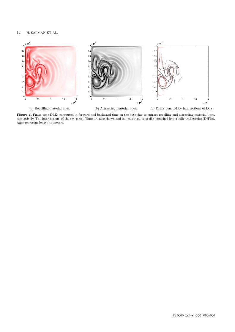
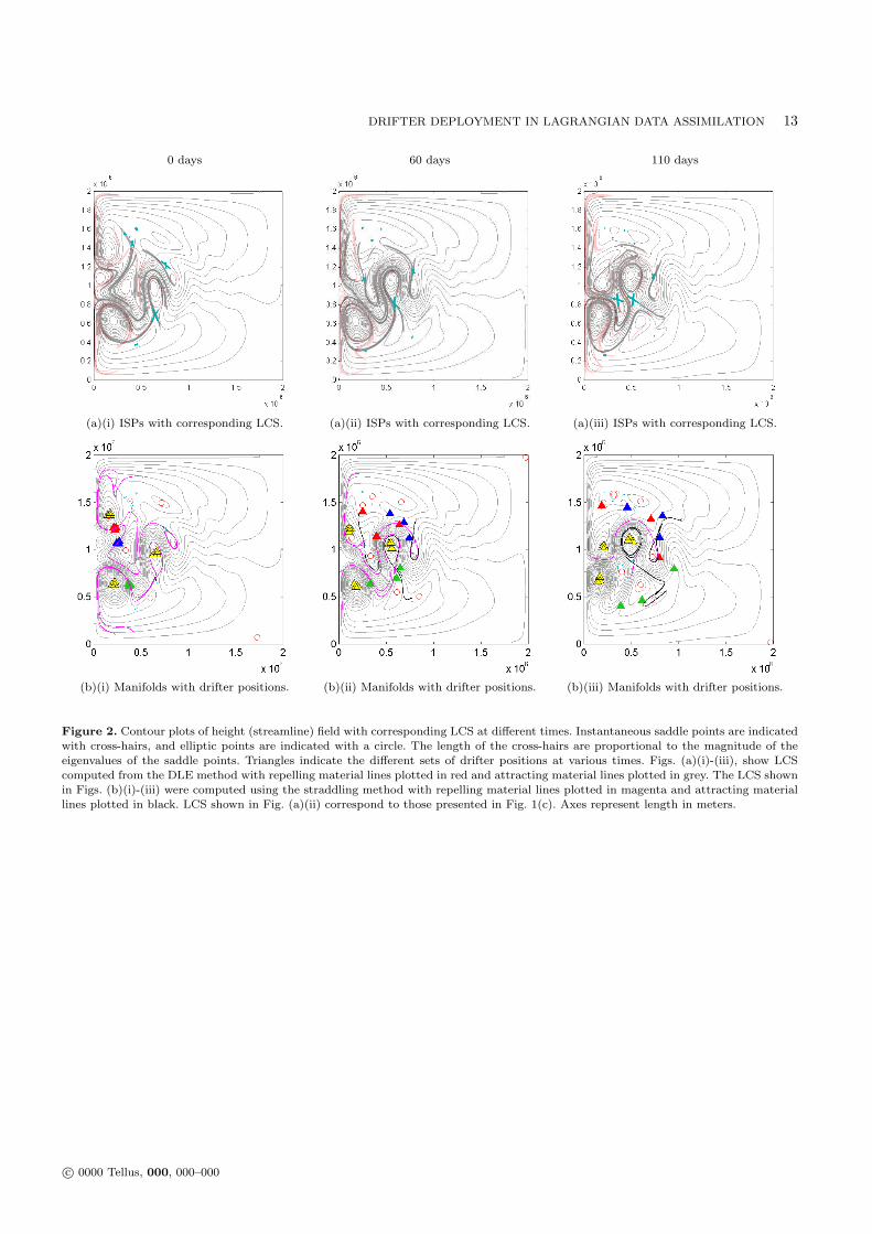
Figure 1 shows plots of the DLEs computed in forwardand backward time at the 60th day of the 13th year. Thetime interval for integration was set to 50 days. Integrationmade in forward time is used to reveal repelling materiallines whilst integration made in backward time is used toreveal attracting material lines. These attracting/ repellingmaterial lines are approximate finite-time generalizations ofunstable/stable manifolds of time-periodic flows. They or-chestrate how water parcels are advected by the underlyingflow field and reveal regions that can lead to rapid disper-sion of the drifters. From the figures, we observe that mostof the underlying structure is located close to the westernboundary within the mid-latitude jet. We also notice thatsignificant shearing is present in the flow which gives riseto spurious structures (those with significantly lower valuesof the DLE field). To clarify the structures of most rele-vance, we have re-plotted the two fields in Fig. 1c. A lowerthreshold has been applied in this case to remove most ofthe spurious structures present in Figs. 1a and 1b. Here thepink values depict repelling material lines whilst grey de-pict attracting material lines. The two DLE fields have beenoverlayed on one another to identify regions where the ex-trema of the two fields intersect. Such intersections give apotential indication of where DHTs are located within theflow. We have employed this approach to identify three hy-perbolic trajectories as indicated in Fig. 1c. We note that,in general, the repelling and attracting material lines willintersect at many locations. In selecting the intersectionsshown in Fig. 1c, we have made use of the fact that for ourdouble gyre flow, we expect the DHTs to be located closeto the ISPs. This is illustrated in the corresponding plotsof the instantaneous height (streamline field), shown in Fig.2a, in which the ISPs are indicated by the cross-hairs. Thecross-hairs have been scaled according to the magnitude oftheir respective eigenvalues and indicate that the three tra-jectories we have identified correspond to regions of stronghyperbolicity. We can, therefore, expect rapid dispersion ofthe drifters that straddle the respective repelling materiallines of these DHTs.

In order to refine the computations of the attractingand repelling material lines presented in Fig. 2a, we haveused the method of straddling used by Malhotra and Wig-gins (1998) and also employed in the work of Salman et al.

c© 0000 Tellus, 000, 000–000


(2007) in combination with the DLE method. The idea hereis to initialize a small material line segment close to theDHT and straddling one of its corresponding stable or un-stable directions. For attracting material lines, we initial-ize a segment straddling the stable direction and integrateforward in time. The process is reversed for computing re-pelling material lines with the integration being performedin backward time. Haller and Poje (1998) showed that forgeophysical flows, in which a clear separation exists betweenthe Lagrangian and Eulerian flow time-scales, the stable andunstable directions of the DHTs are approximately alignedwith the stable and unstable eigenvectors of the nearby ISP.We have, therefore, used this property to initialize our linesegments close to the ISPs and straddling the respectiveeigenvectors as required. We point out that while this ap-proach can potentially introduce an error in terms of theinitial placement of the material line with respect to thestructures of interest, the errors converge to zero at an ex-ponential rate with respect to the time of integration. Thisproperty is a characteristic of DHTs and can be exploitedin their computation.

Figure 2b shows plots of the attracting and repellingmaterial lines corresponding to the DHTs identified in Fig.2a. Also presented are the motion of drifters that have beeninitialized in six groups of three. Drifters in three of thegroups are initialized at positions straddling a repelling ma-terial line so that after some time they disperse rapidly asthey encounter the respective DHT. The other three setsof drifters are initialized within the cores of three vortices.These drifters remain in these vortices throughout most ofthe first year. We will use the sets of drifters shown in Fig. 2bto determine how they affect the performance of our LaDAmethod presented in section 2.

4.2 Lagrangian data assimilation

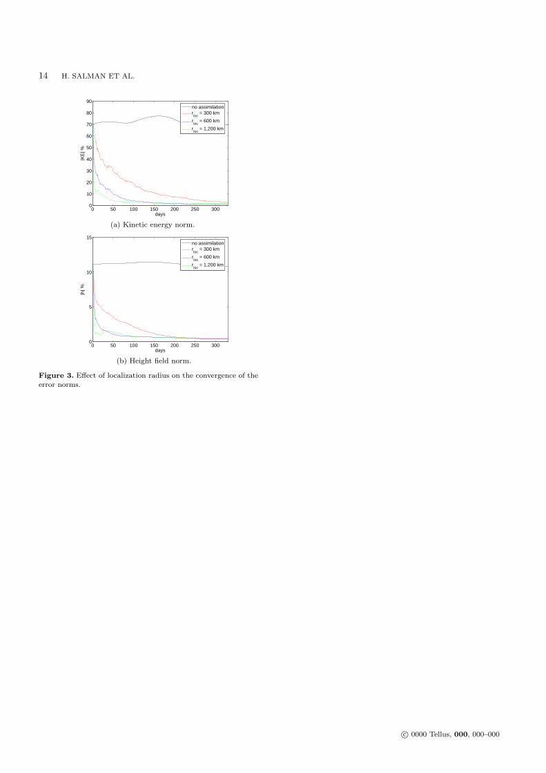
Before presenting assimilation results for our drifter de-ployment strategy, we first need to prescribe several key pa-rameters for our data assimilation simulations. Clearly, themethod will stongly depend on the localization radius em-ployed in our Ensemble Kalman Filter (EnKF). The studyof Salman et al. (2006) indicated that a localization radiusof r

loc= 600km provided optimal results. To verify that this

figure continues to hold for our modified form of the govern-ing flow equations (i.e. with different form of the dissipationterm), we have repeated these assimilation experiments. Asin Salman et al., we have tested three values of r

locand

used 36 drifters uniformly distributed throughout the flowdomain in each case.

Results are presented in Fig. 3 in terms of the timehistory for the kinetic energy and height field norms. Herewe define the error norms for the flow field and the driftersby

|KE|t =

nx−1,ny−1∑i=1,j=1

(uf

i,j − uti,j

)2

+(vf

i,j − vti,j

)2

nx−1,ny−1∑i=1,j=1

(uti,j)

2 + (vti,j)

2

1/2

(17)

|h|t =

nx,ny∑

i=1,j=1

(hf

i,j − hti,j

)2

nx,ny∑

i=1,j=1

(hti,j)

2

1/2

(18)

|xD|t =

ND∑i=1

(xf

D,i − xtD,i

)2

+(yf

D,i − ytD,i

)2

σ2ND

1/2

(19)

where overbars denote ensemble mean quantities. We notethat, for the results to be presented in the remainder of thisstudy, day 0 corresponds to the beginning of the 13th year.All three assimilation experiments show a reduction in theerror norms with respect to the case without assimilation.The results also clearly indicate that as r

locis increased,

the initial rate of convergence in both norms also increases.However, while the convergence for both r

loc= 300km and

rloc

= 600km is more or less monotonic over the length ofthe simulation, this is clearly not the case for r

loc= 1200km.

This is best seen in the norm of the height field which revealsa gradual increase at around 25 days. Moreover, the normin the kinetic energy field at 330 days with r

loc= 1200km

is greater than the case with rloc

= 600km. As pointed outby Hamill et al. (2001), this degradation in the convergenceof the method for large r

lococcurs as a result of spurious

noisy correlations that exist in the covariance matrix. Wewill, therefore, use r

loc= 600km in the remainder of this

work which we have clearly shown to be the optimum valuefor our modified system of equations.

A second key parameter that can have an importantimpact on the convergence of the method is the number ofdrifters released into the flow. The previous study conductedby Salman et al. (2006) indicated a value of 36 drifters uni-formly released into the flow provided optimal results. In-creasing the number of drifters beyond this value did notsignificantly alter the results. Given that we are interestedin using our drifter deployment strategy to obtain the bestresults with the fewest possible number of drifters, we haveexplored how reducing the number of uniformly distributeddrifters affected our results. Figure 4 shows the convergenceof the kinetic energy and height flow fields for five differentcases in which the total number of drifters uniformly releasedinto the flow was varied from 4 to 36. The results clearly indi-cate that best results are obtained with 36 drifters. However,the gain made in the convergence of the method diminisheswith an increasing number of drifters. In particular, there isa significant improvement in increasing the drifters from 4to 9 in comparison to improvements made beyond 9 drifters.Given this observation, we have chosen to focus on the use ofnine drifters for our optimal deployment strategy. Our aim isto see how a directed drifter deployment strategy with onlynine drifters will compare with the results obtained with auniform drifter deployment strategy.

The sets of drifters used in our directed drifter deploy-ment studies are those shown in Fig. 2b with their cor-responding initial release locations given in Table 2. Alsoincluded in the table are the initial drifter deployment lo-cations used in the uniform launch with nine drifters. Asstated earlier, six groups of drifters were employed in the di-

c© 0000 Tellus, 000, 000–000

6 H. SALMAN ET AL.

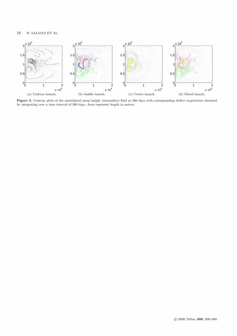
rected drifter deployment with each group containing threedrifters. Three of these groups were deployed so as to strad-dle repelling material lines of associated DHTs whilst theremaining three groups were released within vortex centers.We have divided our directed drifter deployment data assim-ilation experiments using these drifters into three differentcases. In the first case, we considered the set of drifters tar-geting DHTs. In the second case, we considered the set ofdrifters targeting only vortex centers. Finally, in the thirdcase, we employed a drifter released within each of the vor-tex cores and two of the three groups of drifters targetingDHTs. This included drifters 1,2,3,7,8,9,10,13, and 16. A to-tal of nine drifters was used in each one of these assimilationexperiments.

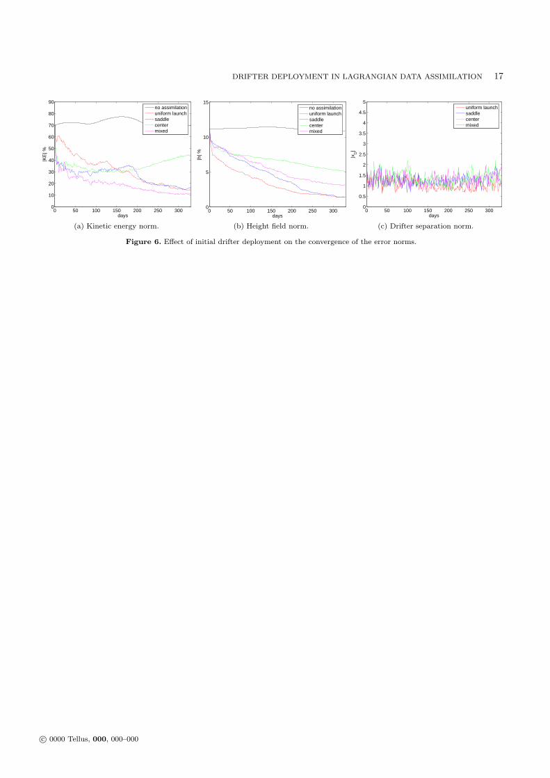
To illustrate the distinctive nature of the drifter mo-tion in the four assimilation experiments (including the casewith nine uniformly released drifters), we have plotted theirtrajectories over the time interval [0,300] days. These areshown in Fig. 5 for each of the uniform, saddle, center, andmixed drifter launch cases. Figure 5a, which corresponds tothe uniform case, shows a good coverage of the flow by thedrifter trajectories and can be directly attributed to the ini-tially disparate drifter placements. The saddle case shownin Fig. 5b illustrates that DHTs can produce rapid drifterdispersion leading to good flow coverage even though thedrifters were initially placed in clusters of three. The centerlaunch (Fig. 5c) shows the least spread in the drifter tra-jectories with drifters being trapped within their respectivevortices. The mixed case is a combination of the center andsaddle cases and produces an intermediate level of disper-sion. We will now begin to analyze how such different driftertrajectories influence the convergence of our LaDA method.

Figure 6 presents results over an assimilation time in-terval of 330 days for the three cases of directed drifter de-ployment described above. Also included for comparison isthe case of uniformly released 3×3 drifters and a case with-out data assimilation. Results for the kinetic energy normshown in Fig. 6a indicate that in all three cases in whicha directed drifter deployment was used, the convergence isinitially much faster than in the case of uniformly releaseddrifters. After a period of about 200 days, however, the vor-tex center launch shows a gradual rise in the norm of thekinetic energy and reveals the poorest performance of thefour assimilation experiments considered. The cause of thisgradual error increase is discussed later in this section. Thecase in which DHTs are targeted, reveals the same level ofconvergence as the uniform case at the end of 330 days.However, by far the best convergence is obtained with themixed launch. Results for the convergence of the height normpresented in Fig. 6b reveal a different trend. In this case,the uniformly released drifters produce the fastest conver-gence with the saddle launch eventually resulting in similarnorms after 330 days. The mixed launch is seen to producea slightly poorer convergence but, as in the kinetic energynorms, the poorest results are obtained with the vortex cen-ters. In all the cases considered above, the assimilated driftertrajectories are seen to track the true drifters as indicatedby the non-dimensionalised drifter error norms presented inFig. 6c.

To understand why the results for the kinetic energyand height field norms have different trends with respect tothe various drifter launch sites, a more detailed inspection

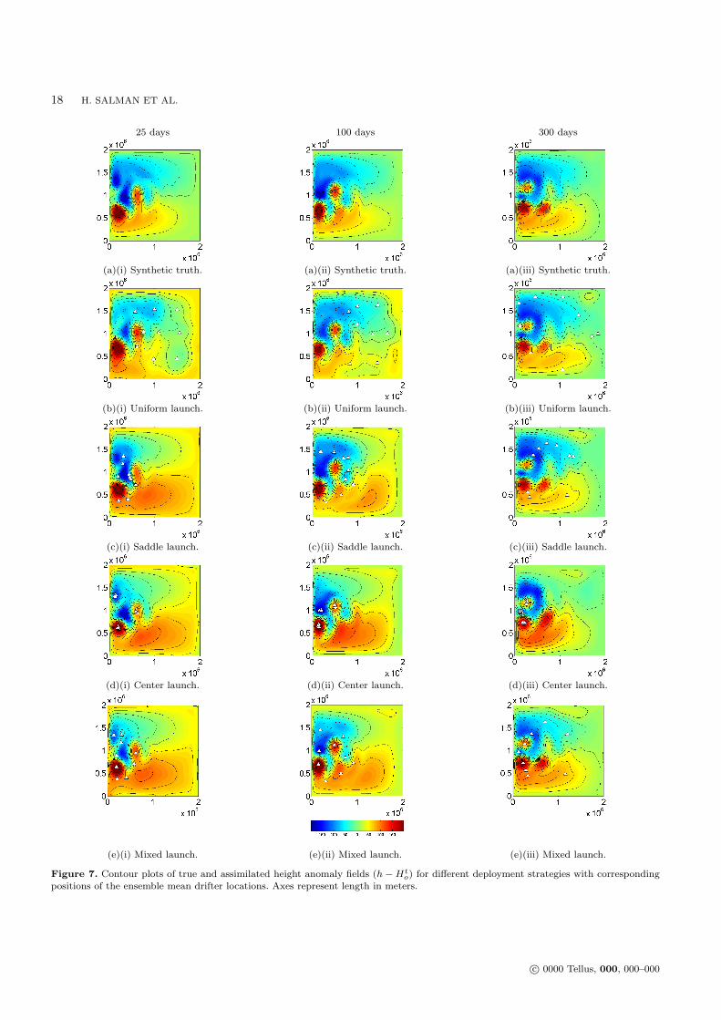
of the assimilated flow field is required. We begin by con-sidering contour plots of the height field. Figure 7 presentscontour plots of the height anomaly at three different timesfor all four assimilation experiments. Also shown in Fig. 7aare the corresponding plots for the control run (synthetictruth). Overlayed on the plots for the cases with assimila-tion are the ensemble mean positions of the nine drifters toillustrate how the flow field is updated by the motion of thedrifters. Results for the case with uniformly released driftersare shown in Fig. 7b. The gradual convergence of the heightfield to that of the control run can be seen from the increas-ing coverage of the flow with negatively valued contours ofthe height anomaly. Results for the saddle launch are shownin Fig. 7c. At earlier times, we observe the corrections areconfined closer to the western boundary where most of thedrifters are initially released. As the drifters disperse, theyprovide more widespread coverage of the flow. Therefore, atlater times, the height anomaly field is qualitatively similarto the uniform case and is consistent with the global errornorms presented in Fig. 6b. Comparing these results withthe case corresponding to the vortex center launch presentedin Fig. 7d reveals some stark differences. In particular, thedrifters remain trapped within the eddies which themselvesremain confined to the western boundary region of the flow.This lack of dispersion in the drifters results in the heightfield being updated only locally. Consequently, the flow closeto the eastern boundary remains with unrealistically highlevels of the height anomaly field. This produces the poorerglobal trend in the norm of the height field observed in Fig.6b. Finally, the results for the mixed launch reveal a trendthat is more characteristic of the saddle case although theheight anomalies are less well represented close to the upperboundary after 300 days.

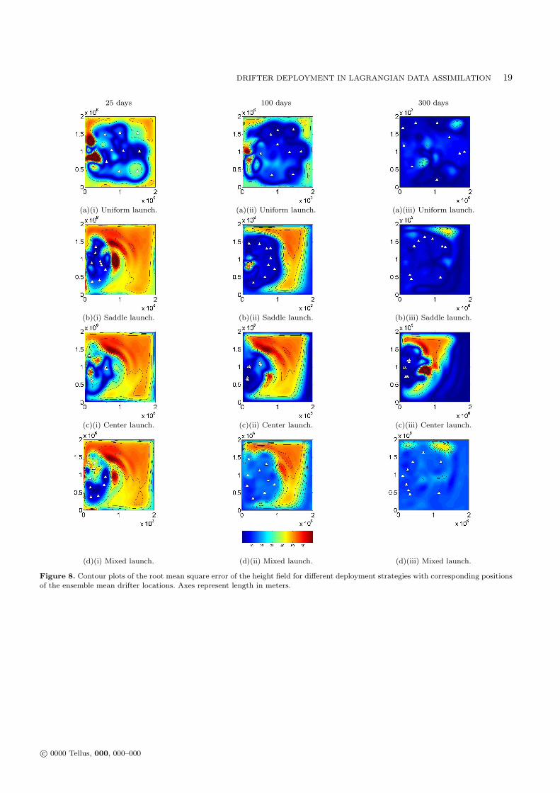
To provide a clearer representation of how errors are re-duced in the four different cases, we have computed contourplots of the root mean square errors of the height field. Theresults are presented in a similar arrangement to that usedin Fig. 7. Considering the case of uniformly released driftersas shown in Fig. 8a, we observe the errors are initially re-duced within the central part of the flow domain and faraway from the boundaries. As time progresses and driftersdisperse, the flow is gradually adjusted in remote regionsincluding the boundaries. By 300 days, the error has beenalmost entirely eliminated. In comparison, the saddle launchpresented in Fig. 8b reveals the errors are initially reducedcloser to the western boundary. As the drifters rapidly dis-perse following their encounter with the respective DHTs,the flow is adjusted until the errors have been uniformly re-duced throughout the flow. The poorer convergence with thecase of vortex centers is very clearly illustrated in Fig. 8c.The results clearly show that a significant part of the flowhas not been adjusted by the data assimilation method. Fi-nally, the mixed case reveals results that are most similar tothe saddle launch albeit that, after 300 days, the overall er-rors are slightly higher. The results presented here are fullyconsistent with those presented in Fig. 7 and clearly illus-trate the impact that different drifter deployment strategieshave on the assimilated flow field.

We will now consider how errors associated with thevelocity field are influenced by assimilating different drifterdata. In particular, we want to identify why the errors ob-served in Fig. 6a for the norms of the kinetic energy have a

c© 0000 Tellus, 000, 000–000


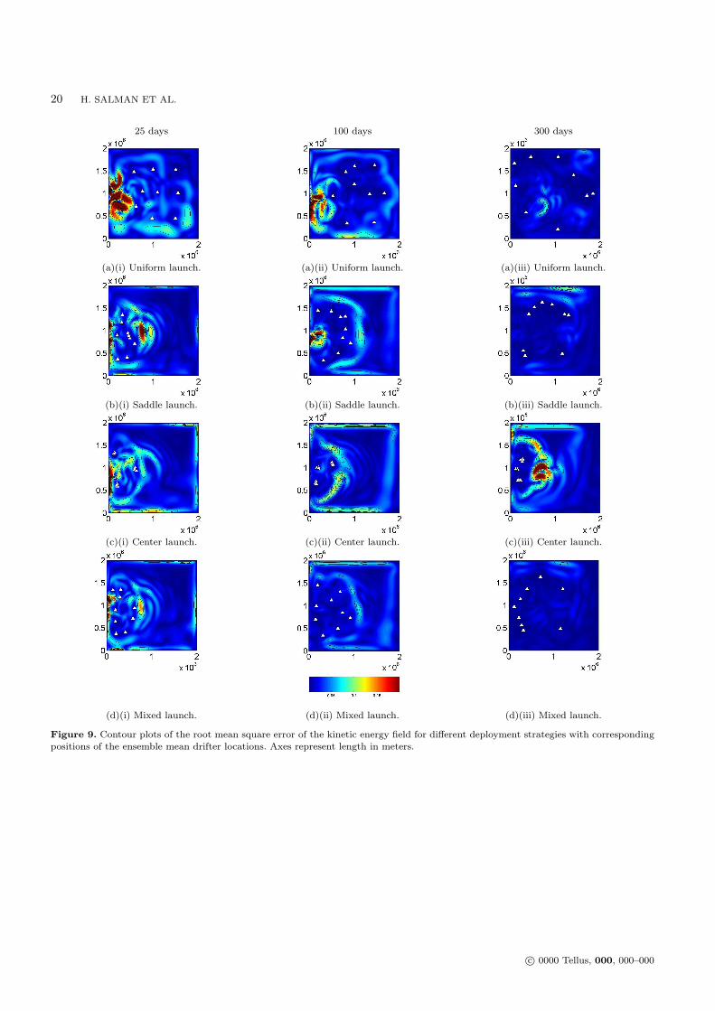
different trend from the norms of the height field presentedin Fig. 6b. Contour plots of the root mean square errors ofthe kinetic energy field are presented in Fig. 9. A featurewhich immediately stands out from the plots presented hereis that, even at the very early stages of the data assimila-tion, the errors are primarily localized close to the separa-tion point of the western boundary currents. This region ofthe flow is highly active containing the formation of vor-tices from the unsteady meandering jet. Therefore, unlikethe errors for the height field, the errors for the velocity arelocalized to energetic regions of the flow. Recognizing thiskey point helps to explain the differences observed in the be-havior of the norms for these two quantities. Now focusingon the case of the uniform drifter launch shown in Fig. 9a,we observe that the drifters are initially placed in the openocean far away from the energetic western boundary eddies.This results in a slight delay in the correction of this part ofthe flow, as shown in Figs. 9a(i) and 9a(ii), and explains theslower initial convergence observed in Fig. 6a relative to thethree directed drifter deployment cases. The saddle launchon the other hand, as with the center and mixed launches,show that, after 25 days, a significant percentage of the er-ror has been removed (see Figs. 9-b(i),c(i),d(i)). In all threecases, the placement of the drifters closer to the westernboundary results in improved convergence at earlier times.For longer times, the dispersion of the drifters in the saddlecase helps to eliminate almost all of the errors. The centerlaunch on the other hand degrades after a sufficiently longtime. The problem is attributed to an eddy that forms inthe region where the maximum errors are seen in Fig. 9c(iii)(see also Fig. 7d(iii)). Without sufficient drifter dispersion,the eddies containing the drifters are well represented whileother energetic eddies remote from the drifters can not becorrectly forecast. Best results for the kinetic energy errorsare, however, predicted with the mixed launch as shown inFig. 9d. In this case, drifters released within the eddies helpto suppress errors within these energetic regions of the flowwhilst errors in remote regions can be corrected by the dis-persion of the remaining drifters. Therefore, while the saddlelaunch proves to be optimal in removing errors in the heightfield, the mixed launch is most effective at removing errorsin the velocity field.

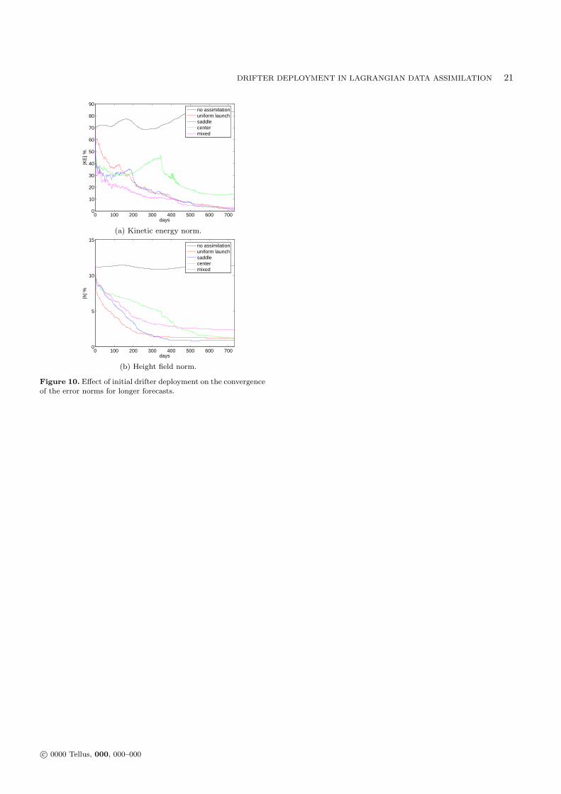
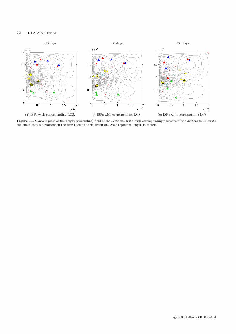
In all the results presented thus far, the center launchhas produced the poorest convergence history in the normsof the flow field. However, if we consider what happens overlonger forecasts, we observe a sudden change in the trends ofthe error norms. This is vividly clear in the results presentedin Fig. 10 in which a sudden and sharp fall in the norms isseen for both the height and the velocity fields at around350 days. After 730 days, despite the drastic reduction inthe error of the velocity field, the errors are still substan-tially higher than the other three cases. The errors in theheight field on the other hand converge to a point where theyare of the same level as the uniform launch case. We have al-ready observed that errors in the height field tend to be moreglobal than errors in the velocity field. The trends observedin Fig. 10b for the height field, therefore, suggest a mech-anism whereby the drifters within the vortex centers musthave undergone rapid dispersion. This is indeed the case asevidenced from plots of the drifter locations at later timesshown in Fig. 11. We observe that at 350 days, one of thedrifters has escaped the vortex within which it was initially

released. The mechanism responsible for the escape of thedrifter is triggered by a bifurcation of the vortex center witha saddle point leading to the annihilation of the vortex. At400 days, a similar fate beholds the drifters trapped withinthe second vortex. Therefore, by 500 days, the drifters havemigrated eastwards assisted by the meandering jet. This ex-pulsion of the drifters to the eastern part of the flow allowserrors in this region of the flow to be corrected which couldnot be accomplished whilst the drifters were trapped withinthe vortices. These results show that forecasts made overtimes that are longer than the Eulerian flow time-scales aredetermined by transformations within the geometry of theflow due to finitely-lived structures. Forecasts made from La-grangian data over longer times will, therefore, be strikinglydifferent from shorter forecasts.

5 Conclusions

We have presented a thorough investigation to demon-strate how judiciously chosen drifter deployment sites canhave a major impact on the convergence of a LaDA methodthat employs an augmented state vector together with anEnKF formulation. This is in part because the method wehave developed corrects the flow field through correlationsobtained from a covariance matrix of the augmented statevector. Since a correlation function is needed to suppressundesirable noisy correlations between drifters and remoteregions of the flow, only the local flow field can be modifiedby a given drifter. Such an approach is becoming standard inalmost all operational forms of the Ensemble Kalman filter.Consequently, the dispersion characteristics of Lagrangiandrifter trajectories, which are governed by the underlyingflow geometry, will strongly influence the performance ofthe method.

We have attempted to quantify the dependence of themethod on these drifter trajectories by extracting LCS ofthe underlying flow field. Such structures uncover the un-derlying flow geometry that directly control the motion ofLagrangian drifters. By using these structures together witha directed drifter deployment strategy that targets vortexcenters or DHTs of the flow, we were able to realize driftertrajectories with contrasting dispersion characteristics. Inthis study, we compared four different launch sites; a uni-form drifter deployment within the ocean basin, a saddlelaunch strategy, a vortex launch strategy, and a mixed com-bination of saddle and vortex center launches. In all cases,we have used a total of nine drifters. The different cases weretested on a twin experiment data assimilation configurationin which the model forecast was generated by perturbingthe initial height field of the control run (synthetic truth)simulation. Our results showed that the convergence of theheight and velocity fields produced by the different launchstrategies had strikingly different time histories. In particu-lar, the mixed launch produced the best convergence for thevelocity field whereas the uniform and saddle launches werebest at minimizing the errors in the height field. These con-trasting behaviors are linked to the different nature of theerrors in the two fields. In general, errors in the height fieldwere associated with an elevated water depth on averageover the entire ocean basin. This was a direct manifestationof the errors introduced in the initial conditions and lead to

c© 0000 Tellus, 000, 000–000

8 H. SALMAN ET AL.

a globally distributed error in the height field. The errorsin the velocity field, on the other hand, are directly corre-lated to the location of the western boundary currents, themeandering midlatitude jet, and the Sverdrup gyres and aremore local in nature. These results suggest that good dis-persion characteristics for the drifters are needed to removeglobal errors while local errors are best removed by target-ing specific energetic regions of the flow. We have also foundthat bifurcations of coherent flow structures in the under-lying flow field can trigger unexpected rapid dispersion ofdrifters initially released within such coherent vortices. Fore-casts made over longer time-scales can, therefore, produceresults that are markedly different from those obtained withshorter forecasts.

The results presented in this study have been ob-tained in the context of a model problem based on a twin-experiment configuration in which the true flow is knowna priori. This simplifying assumption was used to allow usto extract LCS associated with the true flow field whichultimately determines the dispersion characteristics of thedrifters. For the results obtained in this study to be appli-cable in practice, this simplifying assumption needs to berelaxed. In particular, LCS of the forecast should be used todetermine the optimum launch sites of the drifters. In addi-tion, most operational models that are used in forecastingcenters are three-dimensional and exhibit a greater degreeof variability between the forecast and the “truth”. Whilefurther work is needed to address these issues, we point outthat some recent results by Lermusiaux et al. (2005; 2006)indicate that robust LCS can persist even in the presenceof significant uncertainties in the flow field. These resultsprovide a positive sign that the ideas presented in this workmay readily generalize to more complex flow scenarios inwhich the truth is not known a priori.

6 Acknowledgments

H. Salman, and C.K.R.T. Jones were supported bythe Office of Naval Research Grants N00014-93-1-0691 andN00014-03-1-0174; K. Ide was supported by the Office ofNaval Research Grant N00014-04-1-0191. The authors wouldlike to thank Dr. Pierre F.J. Lermusiaux and an anonymousreferee for their valuable comments.

REFERENCES

Aref, H. 1984. Stirring by chaotic advection. J. Fluid Mech. 143,1–21.

Aref, H. and El Naschie, M.S. 1994. Chaos Applied to Fluid Mix-

ing, Pergamon, New York.Bower, A.S. 1991. A simple kinematic mechanism for mixing fluid

parcels across a meandering jet. J. Phys. Oceanogr. 21, 173–180.

Carter, E.F. 1989. Assimilation of Lagrangian data into numericalmodels. Dyn. Atmos. Oceans 13, 335–348.

Coulliette, C. and Wiggins, S. 2000. Intergyre transport in a wind-

driven, quasi-geostrophic double gyre: An application of lobedynamics. Nonlinear Processes in Geophys. 7, 59–85.

Cushman-Roisin, B. 1994. Introduction to Geophysical Fluid Dy-

namics, Prentice Hall.Evensen, G. 1994. Sequential data assimilation with a nonlinear

quasi-geostrophic model using Monte Carlo methods to fore-cast error statistics. J. Geophys. Res. 99, C5, 10 143–10 162.

Evensen, G. 2003. The Ensemble Kalman Filter: theoretical for-

mulation and practical implementation. Ocean Dynamics,53, 343–367.

Gaspari, G. and Cohn, S.E. 1999. Construction of correlationfunctions in two and three dimensions. Quart. J. Roy. Me-

teor. Soc., 125, 723–757.

Gent, P.R. 1993. The energetically consistent shallow-water equa-tions. J. Atmos. Sci., 50, 1323–1325.

Haller, G. and Poje, A.C. 1998. Finite time mixing in aperiodicflows. Physica D, 119, 352–380.

Haller, G. 2001. Distinguished material surfaces and coherent

structures in 3D fluid flows. Physica D, 149, 248–277.Haller, G. 2002. Lagrangian coherent structures from approximate

velocity data. Phys. Fluids A, 14, 1851–1861.Hamill, T.M., Whitaker, J.S. and Snyder, C. 2001. Distance-

Dependent Filtering of Background Error Covariance Esti-mates in an Ensemble Kalman Filter. Mon. Wea. Rev., 129,2776–2790.

Ide, K., Kuznetsov, L. and Jones, C.K.R.T. 2002. Lagrangian dataassimilation for point vortex systems. J. Turbul., 3, 053.

Jones, C.K.R.T. and Winkler, S. 2002. Invariant manifolds and

Lagrangian dynamics in the ocean and atmosphere. In:Handbook of Dynamical Systems, (eds. B. Fiedler), North-Holland, 2, 55–92.

Kamachi, M. and O’Brien, J.J. 1995. Continuous assimilationof drifting buoy trajectory into an equatorial Pacific Ocean

model. J. Mar. Syst., 6, 159–178.Kuznetsov, L., Toner, M., Kirwan, A.D., Jones, C.K.R.T., Kan-

tha, L.H. and Choi, J. 2002. The Loop Current and adjacent

rings delineated by Lagrangian analysis of near-surface flow.J. Mar. Res., 60, 405–429.

Kuznetsov, L., Ide, K. and Jones, C.K.R.T. 2003. A Methodfor Assimilation of Lagrangian Data. Mon. Wea. Rev., 131,2247–2260.

Lermusiaux, P.F.J. and Lekien, F. 2005. Dynamics and La-grangian Coherent Structures in the Ocean and their Uncer-

tainty. Extended Abstract in Dynamical System Methods in

Fluid Dynamics, Oberwolfach Workshop. Jerrold E. Marsden

and Jurgen Scheurle (Eds.), Mathematisches Forschungsin-

stitut Oberwolfach, July 31st - August 6th, 2005, Germany,

19–20.

Lermusiaux, P.F.J., Chiu, C.-S., Gawarkiewicz, G.G., Abbot, P.,Robinson, A.R., Miller, R.N., Haley, P.J., Leslie, W.G., Ma-jumdar, S.J., Pang, A. and Lekien, F. 2006. Quantifying Un-

certainities in Ocean Predictions. Oceanography. In: Special

issue on “Advances in Computational Oceanography”, (eds.

T. Paluszkiewicz and S. Harper), 19, 92–105.Malhotra, N. and Wiggins, S. 1998. Geometric structures, lobe

dynamics, and Lagrangian transport in flows with aperiodic

time-dependence, with applications to Rossby wave flow. J.

Nonlinear Sci., 8, 401–456.Mancho, A.M., Small, D. and Wiggins, S. 2004. Computation of

hyperbolic trajectories and their stable and unstable mani-folds for oceanographic flows represented as data sets. Non.

Process. Geophy., 11, 17–33.Molcard, A., Piterbarg, L.I., Griffa, A., Ozgokmen, T.M. and

Mariano, A.J. 2003. Assimilation of drifter observations for

the reconstruction of the Eulerian circulation field. J. Geo-

phys. Res., 108, C3, 1 1–1 21.

Molcard, A., Poje, A.C. and Ozgokmen, T.M. 2006. Directeddrifter launch strategies for Lagrangian data assimilation us-ing hyperbolic trajectories. Ocean Modeling, 12, 237–267.

Ozgokmen, T.M., Griffa, A. and Mariano, A.J. 2000. On the Pre-dictability of Lagrangian Trajectories in the Ocean. J. At-

mos. Oceanic Technol., 17, 366–383.Ozgokmen, T.M., Molcard, A., Chin, T.M., Piterbarg, L.I. and

c© 0000 Tellus, 000, 000–000


Griffa, A. 2003. Assimilation of drifter observations in prim-itive equation models of midlatitude ocean circulation. J.

Geophys. Res., 108, C7, 31 1–31 17.

Pedlosky, J. 1986. Geophysical Fluid Dynamics, 2d ed. Springer-Verlag.

Poje, A. and Haller, G. 1999. Geometry of cross-stream mixingin a double-gyre ocean model. J. Phys. Oceanogr. 29, 1649–1665.

Poje, A.C., Toner, M., Kirwan, A.D. and Jones, C.K.R.T. 2002.Drifter launch strategies based on Lagrangian templates. J.

Phys. Oceanogr., 32, 1855–1869.Salman, H., Kuznetov, L., Jones, C.K.R.T. and Ide, K. 2006.

A method for assimilating Lagrangian data into a shallow-

water equation ocean model. Mon. Wea. Rev., 134, 1081–1101.

Salman, H., Hesthaven, J.S., Warburton, T. and Haller, G. 2007.Predicting transport by Lagrangian coherent structures witha high order method. Theor. & Comp. Fluid Dynam., 21,

39–58.Schar, C. and Smith, R.B. 1993. Shallow-water flow past isolated

topography. Part I: Vorticity production and wake forma-

tion. J. Atmos. Sci., 50, 1373–1400.Shchepetkin, A.F. and O’Brien, J.J. 1996. A method for assimi-

lating Lagrangian data into a shallow-water equation oceanmodel. Mon. Wea. Rev., 124, 1285–1300.

Toner, M. and Poje, A.C. 2004. Lagrangian velocity statistics of

directed launch strategies in a Gulf of Mexico model. Non.

Process. Geophy., 11, 35–46.

Wiggins, S. 2005. The dynamical systems approach to Lagrangiantransport in oceanic flows. Ann. Rev. Fluid Mech., 37, 295–328.

c© 0000 Tellus, 000, 000–000

10 H. SALMAN ET AL.

Table 1. Parameters prescribed for the reduced gravity shallow

water system of equations.

Property Value

Lx 2000 km

Ly 2000 kmfo 6 × 10−5s−1

β 2 × 10−11 m−1s−1

Ho 500 mg′ 0.02 ms−2

ρ 1000 kg m−3

τo 0.05 Nm−2

∆x 20 km

∆y 20 km∆t 12 minutes

ν 400 m2s−1

Table 2. Initial drifter locations used in the uniform launch and

directed launch simulations.

Launch method Drifter Number Coordinates (km)

Saddle (red) 1 (220.5,1211.0)2 (230.5,1231.0)

3 (205.5,1231.0)Saddle (blue) 4 (238.5,1066.8)

5 (263.5,1062.0)

6 (270.5,1087.0)Saddle (green) 7 (365.0,617.5)

8 (390.0,622.5)

9 (365.0,642.5)

Center (yellow) 10 (143.4,1361.5)11 (168.4,1361.5)

12 (168.4,1386.5)13 (188.5,624.7)14 (218.5,624.7)15 (218.5,654.7)16 (629.5,950.0)17 (664.5,950.0)18 (664.5,980.0)

Uniform 19 (500.0,500.0)20 (1000.0,500.0)21 (1500.0,500.0)22 (500.0,1000.0)23 (1000.0,1000.0)24 (1500.0,1000.0)25 (500.0,1500.0)26 (1000.0,1500.0)27 (1500.0,1500.0)

c© 0000 Tellus, 000, 000–000


Figure 1: Finite time DLEs computed in forward and backward time on the 60th day to extract repelling and attracting material

lines, respectively. The intersections of the two sets of lines are also shown and indicate regions of distinguishedhyperbolic trajectories (DHTs). Axes represent length in meters.

Figure 2: Contour plots of height (streamline) field with corresponding LCS at different times. Instantaneous saddle points areindicated with cross-hairs, and elliptic points are indicated with a circle. The length of the cross-hairs are proportional

to the magnitude of the eigenvalues of the saddle points. Triangles indicate the different sets of drifter positions atvarious times. Figs. (a)(i)-(iii), show LCS computed from the DLE method with repelling material lines plotted in redand attracting material lines plotted in grey. The LCS shown in Figs. (b)(i)-(iii) were computed using the straddlingmethod with repelling material lines plotted in magenta and attracting material lines plotted in black. LCS shown inFig. (a)(ii) correspond to those presented in Fig. 1(c). Axes represent length in meters.

Figure 3: Effect of localization radius on the convergence of the error norms.

Figure 4: Effect of number of drifters used on the convergence of the error norms.

Figure 5: Contour plots of the assimilated mean height (streamline) field at 300 days with corresponding drifter trajectoriesobtained by integrating over a time interval of 300 days. Axes represent length in meters.

Figure 6: Effect of initial drifter deployment on the convergence of the error norms.

Figure 7: Contour plots of true and assimilated height anomaly fields (h − Hto) for different deployment strategies with corre-

sponding positions of the ensemble mean drifter locations. Axes represent length in meters.

Figure 8: Contour plots of the root mean square error of the height field for different deployment strategies with correspondingpositions of the ensemble mean drifter locations. Axes represent length in meters.

Figure 9: Contour plots of the root mean square error of the kinetic energy field for different deployment strategies withcorresponding positions of the ensemble mean drifter locations. Axes represent length in meters.

Figure 10: Effect of initial drifter deployment on the convergence of the error norms for longer forecasts.

Figure 11: Contour plots of the height (streamline) field of the synthetic truth with corresponding positions of the drifters to

illustrate the affect that bifurcations in the flow have on their evolution. Axes represent length in meters.

c© 0000 Tellus, 000, 000–000

12 H. SALMAN ET AL.

(a) Repelling material lines. (b) Attracting material lines. (c) DHTs denoted by intersections of LCS.

Figure 1. Finite time DLEs computed in forward and backward time on the 60th day to extract repelling and attracting material lines,respectively. The intersections of the two sets of lines are also shown and indicate regions of distinguished hyperbolic trajectories (DHTs).

Axes represent length in meters.

c© 0000 Tellus, 000, 000–000


0 days 60 days 110 days

(a)(i) ISPs with corresponding LCS. (a)(ii) ISPs with corresponding LCS. (a)(iii) ISPs with corresponding LCS.

(b)(i) Manifolds with drifter positions. (b)(ii) Manifolds with drifter positions. (b)(iii) Manifolds with drifter positions.

Figure 2. Contour plots of height (streamline) field with corresponding LCS at different times. Instantaneous saddle points are indicatedwith cross-hairs, and elliptic points are indicated with a circle. The length of the cross-hairs are proportional to the magnitude of the

eigenvalues of the saddle points. Triangles indicate the different sets of drifter positions at various times. Figs. (a)(i)-(iii), show LCScomputed from the DLE method with repelling material lines plotted in red and attracting material lines plotted in grey. The LCS shownin Figs. (b)(i)-(iii) were computed using the straddling method with repelling material lines plotted in magenta and attracting material

lines plotted in black. LCS shown in Fig. (a)(ii) correspond to those presented in Fig. 1(c). Axes represent length in meters.

c© 0000 Tellus, 000, 000–000

14 H. SALMAN ET AL.

0 50 100 150 200 250 3000

10

20

30

40

50

60

70

80

90

days

|KE

| %

no assimilationrloc

= 300 km

rloc

= 600 km

rloc

= 1,200 km

(a) Kinetic energy norm.

0 50 100 150 200 250 3000

5

10

15

days

|h| %

no assimilationrloc

= 300 km

rloc

= 600 km

rloc

= 1,200 km

(b) Height field norm.

Figure 3. Effect of localization radius on the convergence of theerror norms.

c© 0000 Tellus, 000, 000–000


0 50 100 150 200 250 3000

10

20

30

40

50

60

70

80

90

days

|KE

| %

no assimilation2x2 drifters3x3 drifters4x4 drifters5x5 drifters6x6 drifters


0 50 100 150 200 250 3000

5

10

15

days

|h| %

no assimilation2x2 drifters3x3 drifters4x4 drifters5x5 drifters6x6 drifters


Figure 4. Effect of number of drifters used on the convergenceof the error norms.

c© 0000 Tellus, 000, 000–000

16 H. SALMAN ET AL.

0 1 2

x 106

0

0.5

1

1.5

2x 10

6

(a) Uniform launch.

0 1 2

x 106

0

0.5

1

1.5

2x 10

6

(b) Saddle launch.

0 1 2

x 106

0

0.5

1

1.5

2x 10

6

(c) Center launch.

0 1 2

x 106

0

0.5

1

1.5

2x 10

6

(d) Mixed launch.

Figure 5. Contour plots of the assimilated mean height (streamline) field at 300 days with corresponding drifter trajectories obtainedby integrating over a time interval of 300 days. Axes represent length in meters.

c© 0000 Tellus, 000, 000–000


0 50 100 150 200 250 3000

10

20

30

40

50

60

70

80

90

days

|KE

| %

no assimilationuniform launchsaddlecentermixed


0 50 100 150 200 250 3000

5

10

15

days

|h| %



0 50 100 150 200 250 3000

0.5

1

1.5

2

2.5

3

3.5

4

4.5

5

days

|xD|

uniform launchsaddlecentermixed

(c) Drifter separation norm.

Figure 6. Effect of initial drifter deployment on the convergence of the error norms.

c© 0000 Tellus, 000, 000–000

18 H. SALMAN ET AL.


(a)(i) Synthetic truth. (a)(ii) Synthetic truth. (a)(iii) Synthetic truth.

(b)(i) Uniform launch. (b)(ii) Uniform launch. (b)(iii) Uniform launch.

(c)(i) Saddle launch. (c)(ii) Saddle launch. (c)(iii) Saddle launch.

(d)(i) Center launch. (d)(ii) Center launch. (d)(iii) Center launch.

(e)(i) Mixed launch. (e)(ii) Mixed launch. (e)(iii) Mixed launch.

Figure 7. Contour plots of true and assimilated height anomaly fields (h − Hto) for different deployment strategies with corresponding

positions of the ensemble mean drifter locations. Axes represent length in meters.

c© 0000 Tellus, 000, 000–000



(a)(i) Uniform launch. (a)(ii) Uniform launch. (a)(iii) Uniform launch.

(b)(i) Saddle launch. (b)(ii) Saddle launch. (b)(iii) Saddle launch.

(c)(i) Center launch. (c)(ii) Center launch. (c)(iii) Center launch.

(d)(i) Mixed launch. (d)(ii) Mixed launch. (d)(iii) Mixed launch.

Figure 8. Contour plots of the root mean square error of the height field for different deployment strategies with corresponding positionsof the ensemble mean drifter locations. Axes represent length in meters.

c© 0000 Tellus, 000, 000–000

20 H. SALMAN ET AL.


(a)(i) Uniform launch. (a)(ii) Uniform launch. (a)(iii) Uniform launch.

(b)(i) Saddle launch. (b)(ii) Saddle launch. (b)(iii) Saddle launch.

(c)(i) Center launch. (c)(ii) Center launch. (c)(iii) Center launch.

(d)(i) Mixed launch. (d)(ii) Mixed launch. (d)(iii) Mixed launch.

Figure 9. Contour plots of the root mean square error of the kinetic energy field for different deployment strategies with correspondingpositions of the ensemble mean drifter locations. Axes represent length in meters.

c© 0000 Tellus, 000, 000–000


0 100 200 300 400 500 600 7000

10

20

30

40

50

60

70

80

90

days

|KE

| %



0 100 200 300 400 500 600 7000

5

10

15

days

|h| %



Figure 10. Effect of initial drifter deployment on the convergenceof the error norms for longer forecasts.

c© 0000 Tellus, 000, 000–000

22 H. SALMAN ET AL.


(a) ISPs with corresponding LCS. (b) ISPs with corresponding LCS. (c) ISPs with corresponding LCS.

Figure 11. Contour plots of the height (streamline) field of the synthetic truth with corresponding positions of the drifters to illustratethe affect that bifurcations in the flow have on their evolution. Axes represent length in meters.

c© 0000 Tellus, 000, 000–000

using flow geometry for drifter deployment in … flow geometry for drifter deployment in ... the...

Documents