Using arguments for making and explaining

decisions

Leila Amgoud ∗ Henri Prade

Institut de Recherche en Informatique de Toulouse, IRIT-UPS,118 route de Narbonne, 31062 Toulouse, Cedex, France

Abstract

Arguments play two different roles in day life decisions, as well as in the discussionof more crucial issues. Namely, they help to select one or several alternatives, or toexplain and justify an already adopted choice.

This paper proposes the first general and abstract argument-based framework fordecision making. This framework follows two main steps. At the first step, argu-ments for beliefs and arguments for options are built and evaluated using classicalacceptability semantics. At the second step, pairs of options are compared usingdecision principles. Decision principles are based on the accepted arguments sup-porting the options. Three classes of decision principles are distinguished: unipolar,bipolar or non-polar principles depending on whether i) only arguments pro or onlyarguments con, or ii) both types, or iii) an aggregation of them into a meta-argumentare used. The abstract model is then instantiated by expressing formally the mentalstates (beliefs and preferences) of a decision maker. In the proposed framework,information is given in the form of a stratified set of beliefs. The bipolar nature ofpreferences is emphasized by making an explicit distinction between prioritized goalsto be pursued, and prioritized rejections that are stumbling blocks to be avoided.A typology that identifies four types of argument is also proposed. Indeed, eachdecision is supported by arguments emphasizing its positive consequences in termsof goals certainly satisfied and rejections certainly avoided. A decision can also beattacked by arguments emphasizing its negative consequences in terms of certainlymissed goals, or rejections certainly led to by that decision. Finally, this paper artic-ulates the optimistic and pessimistic decision criteria defined in qualitative decisionmaking under uncertainty, in terms of an argumentation process. Similarly, differentdecision principles identified in multiple criteria decision making are restated in ourargumentation-based framework.

Key words: Decision making, Argumentation.

Preprint submitted to Elsevier 13 November 2008

1 Introduction

Decision making, often viewed as a form of reasoning toward action, has raisedthe interest of many scholars including philosophers, economists, psychologists,and computer scientists for a long time. Any decision problem amounts to se-lecting the “best” or sufficiently “good” action(s) that are feasible among dif-ferent alternatives, given some available information about the current stateof the world and the consequences of potential actions. Note that availableinformation may be incomplete or pervaded with uncertainty. Besides, thegoodness of an action is judged by estimating, maybe by means of severalcriteria, how much its possible consequences fit the preferences or the inten-tions of the decision maker. This agent is assumed to behave in a rational way[42,43,49], at least in the sense that his decisions should be as much as pos-sible consistent with his preferences. However, we may have a more requiringview of rationality, such as demanding for the conformity of decision maker’sbehavior with postulates describing how a rational agent should behave [45].

Decision problems have been considered from different points of view. Wemay distinguish two main trends, which are currently influencing researchin artificial intelligence (AI): classical decision theory on the one hand, andcognitively-oriented approaches such as practical reasoning or beliefs-desires-intentions (BDI) settings on the other hand.

1.1 Classical decision making vs. practical reasoning

Classical decision theory, as developed mainly by economists, has focused onmaking clear what is a rational decision maker. Thus, they have looked forprinciples for comparing different alternatives. A particular decision principle,such as the classical expected utility [45], should then be justified on the ba-sis of a set of rationality postulates to which the preference relation betweenactions should obey. This means that in this approach, rationality is capturedthrough a set of postulates that describe what is a rational decision behavior.Moreover, a minimal set of postulates is identified in such a way that it corre-sponds to a unique decision principle. The inputs of this approach are a set ofcandidate actions, and a function that assesses the value of their consequenceswhen the actions are performed in a given state, together with complete or par-tial information about the current state of the world. In other words, such an

⋆ The present paper unifies and develops the content of several conference papers[3,8–10].∗ Corresponding author:

Email address: amgoud@irit.fr (Leila Amgoud).URL: http://www.irit.fr/ Leila.Amgoud/ (Leila Amgoud).

2

approach distinguishes between knowledge and preferences, which are respec-tively encoded in practice by a distribution function assessing the plausibilityof the different states of the world, and by a utility function encoding pref-erences by estimating how good a consequence is. The output is a preferencerelation between actions encoded by the associated principle. Note that suchan approach aims at rank-ordering a group of candidate actions rather thanfocusing on a candidate action individually. Moreover, the candidate actionsare supposed to be feasible. Roughly speaking, we may distinguish two groupsof works in AI dealing with decision that follow the above type of approach.The first group is represented by researches using Bayesian networks [41], andworks on planning under uncertainty (e.g. [22]). Besides, some AI works haveaimed at developing more qualitative frameworks for decision, but still alongthe same line of thoughts (e.g. [23,28,47]).

Other researchers in AI, working on practical reasoning, starting with thegeneric question “what is the right thing to do for an agent in a given situa-tion” [42,44], have proposed a two steps process to answer this question. Thefirst step, often called deliberation [49], consists of identifying the goals of theagent. In the second step, they look for ways of achieving those goals, i.e. forplans, and thus for intermediary goals and sub-plans. Such an approach raisesissues such as: how are goals generated ? are actions feasible ? do actionshave undesirable consequences ? are sub-plans compatible ? are there alterna-tive plans for achieving a given goal, ... In [17], it has been argued that thiscan be done by representing the cognitive states, namely agent’s beliefs, de-sires and intentions (thus the so-called BDI architecture). This requires a richknowledge/preference representation setting, which contrasts with the classi-cal decision setting that directly uses an uncertainty distribution (a probabilitydistribution in the case of expected utility), and a utility (value) function. Be-sides, the deliberation step is merely an inference problem since it amounts tofinding a set of desires that are justified on the basis of the current state ofthe world and of conditional desires. Checking if a plan is feasible and doesnot lead to bad consequences is still a matter of inference. A decision problemonly occurs when several plans or sub-plans are possible, and one of them hasto be chosen. This latter issue may be viewed as a classical decision problem.What is worth noticing in most works on practical reasoning is the use ofargument schemes for providing reasons for choosing or discarding an action(e.g. [31,36]). For instance, an action may be considered as potentially usefulon the basis of the so-called practical syllogism [48]:

• G is a goal for agent X• Doing action A is sufficient for agent X to carry out goal G• Then, agent X ought to do action A

The above syllogism is in essence already an argument in favor of doing actionA. However, this does not mean that the action is warranted, since other argu-

3

ments (called counter-arguments) may be built or provided against the action.Those counter-arguments refer to critical questions identified in [48] for theabove syllogism. In particular, relevant questions are “Are there alternativeways of realizing G?”, “Is doing A feasible?”, “Has agent X other goals thanG?”, “Are there other consequences of doing A which should be taken intoaccount?”. Recently in [11,12], the above syllogism has been extended to ex-plicitly take into account the reference to ethical values in arguments. Anyway,the idea of using arguments for justifying or discarding candidate decisions iscertainty very old, and its account in the literature at least dates back to Aris-totle. See also Benjamin Franklin [34] for an early precise account on the wayof balancing arguments pro and con a choice, more than two hundred yearsago.

1.2 Argumentation and decision making

Generally speaking, argumentation is a reasoning model based on the con-struction and the evaluation of interacting arguments. Those arguments areintended to support / explain / attack statements that can be decisions, opin-ions, ... Argumentation has been used for different purposes [1], such as non-monotonic reasoning (e.g. [29]). Indeed, several frameworks have been devel-oped for handling inconsistency in knowledge bases (e.g. [2,4,14]). Moreover,it has been shown that such an approach is general enough to capture differentexisting approaches for nonmonotonic reasoning [29]. Argumentation has alsobeen extensively used for modeling different kinds of dialogues, in particularpersuasion (e.g. [6]), and negotiation (e.g. [38]). Indeed, an argumentation-based approach for negotiation has the advantage of exchanging in addition tooffers, reasons that support these offers. These reasons may lead their receiversto change their preferences. Consequently, an agreement may be more easilyreached with such approaches, when in other approaches (where agent’s prefer-ences are fixed) negotiation may fail. Adopting such an approach in a decisionproblem would have some obvious benefits. Indeed, not only would the userbe provided with a “good” choice, but also with the reasons underlying thisrecommendation, in a format that is easy to grasp. Note that each potentialchoice usually has pros and cons of various strengths. Argumentation-baseddecision making is expected to be more akin with the way humans deliberateand finally make or also understand a choice. This has been pointed out for along time (see e.g. [34]).

4

1.3 Contribution of the paper

In this paper we deal with an argumentative view of decision making, thusfocusing on the issue of justifying the best decision to make in a given situ-ation, and leaving aside the other related aspects of practical reasoning suchas goal generation, feasibility, and planning. It is why we remain close to theclassical view of decision, but now discussed in terms of arguments. The ideaof articulating decisions on the basis of arguments is relevant for differentdecision problems or approaches such as decision making under uncertainty,multiple criteria decisions, or rule-based decisions. These problems are usuallyhandled separately, and until recently without a close reference to argumen-tation. In practical applications, for instance in medical domain, the decisionto be made has to be chosen under incomplete or uncertain information, thepotential results of candidate decisions are evaluated from different criteria.Moreover, there may exist some expertise in the form of decision rules that as-sociate possible decisions to given contexts. This makes the different decisionproblems somewhat related, and consequently a unified argumentation-basedmodel is needed. This paper proposes such a model.

This paper proposes the first general, and abstract argument-based frame-work for decision making. This framework follows two main steps. At the firststep, arguments for beliefs and arguments for options are built and evaluatedusing classical acceptability semantics. At the second step, pairs of optionsare compared using decision principles. Decision principles are based on theaccepted arguments supporting the options. Three classes of decision princi-ples are distinguished: unipolar, bipolar or non-polar principles depending onwhether i) only arguments pro or only arguments con, or ii) both types, or iii)an aggregation of them into a meta-argument are used. The abstract model isthen instantiated by expressing formally the mental states (beliefs and pref-erences) of a decision maker. In the proposed framework, information is givenin the form of a stratified set of beliefs. The bipolar nature of preferences isemphasized by making an explicit distinction between prioritized goals to bepursued, and prioritized rejections that are stumbling blocks to be avoided. Atypology that identifies four types of argument is also proposed. Indeed, eachdecision is supported by arguments emphasizing its positive consequences interms of goals certainly satisfied and rejections certainly avoided. A decisioncan also be attacked by arguments emphasizing its negative consequences interms of certainly missed goals, or rejections certainly led to by that decision.Another contribution of the paper consists of applying the general frameworkto decision making under uncertainty and to multiple criteria decision. Properchoices of decision principles are shown to be equivalent to known qualitativedecision approaches.

The paper is organized as follows: Section 2 presents an abstract framework

5

for decision making. Section 3 discusses a typology of arguments supportingor attacking candidate decisions. Section 4 applies the abstract framework tomultiple criteria decision making, and section 5 applies the framework to de-cision making under uncertainty. Section 6 compares our approach to existingworks on argumentation-based decision making, and section 7 is devoted tosome concluding remarks and perspectives.

2 A general framework for argumentative decision making

Solving a decision problem amounts to defining a pre-ordering, usually a com-plete one, on a set D of possible options (or candidate decisions), on the basisof the different consequences of each decision. Let us illustrate this problemthrough a simple example borrowed from [32].

Example 1 (Having or not a surgery) The example is about having a surgery(sg) or not (¬sg), knowing that the patient has colonic polyps. The knowledgebase contains the following information:

• having a surgery has side-effects,• not having surgery avoids having side-effects,• when having a cancer, having a surgery avoids loss of life,• if a patient has cancer and has no surgery, the patient would lose his life,• the patient has colonic polyps,• having colonic polyps may lead to cancer.

In addition to the above knowledge, the patient has also some goals like: “noside effects” and “to not lose his life”. Obviously it is more important for himto not lose his life than to not have side effects.

In what follows, L will denote a logical language. From L, a finite set D =d1, . . . , dn of n options is identified. Note that an option di may be a con-junction of other options in D. Let us, for instance, assume that an agentwants a drink and has to choose between tea, milk or both. Thus, there arethree options: d1 : tea, d2 : milk and d3 : tea and milk. In Example 1, the setD contains only two options: d1 : sg and d2 : ¬sg.

Argumentation is used in this paper for ordering the set D. An argumentation-based decision process can be decomposed into the following steps:

(1) Constructing arguments in favor/against statements (pertaining to be-liefs or decisions)

(2) Evaluating the strength of each argument

6

(3) Determining the different conflicts among arguments(4) Evaluating the acceptability of arguments(5) Comparing decisions on the basis of relevant “accepted” arguments

Note that the first four steps globally correspond to an “inference problem” inwhich one looks for accepted arguments, and consequently warranted beliefs.At this step, one only knows what is the quality of arguments in favor/againstcandidate decisions, but the “best” candidate decision is not determined yet.The last step answers this question once a decision principle is chosen.

2.1 Types of arguments

As shown in Example 1, decisions are made on the basis of available knowledgeand the preferences of the decision maker. Thus, two categories of argumentsare distinguished: i) epistemic arguments justifying beliefs and are themselvesbased only on beliefs, and ii) practical arguments justifying options and arebuilt from both beliefs and preferences/goals. Note that a practical argumentmay highlight either a positive feature of a candidate decision, supporting thusthat decision, or a negative one, attacking thus the decision.

Example 2 (Example 1 cont.) In this example, α = [“the patient has colonicpolyps”, and “having colonic polyps may lead to cancer”] is considered as anargument for believing that the patient may have cancer. This epistemic ar-gument involves only beliefs. While δ1 = [“the patient may have a cancer”,“when having a cancer, having a surgery avoids loss of life”] is an argumentfor having a surgery. This is a practical argument since it supports the op-tion “having a surgery”. Note that such argument involves both beliefs andpreferences. Similarly, δ2 = [“not having surgery avoids having side-effects”]is a practical argument in favor of “not having a surgery”. However, the twopractical arguments δ3 = [“having a surgery has side-effects”] and δ4 = [“thepatient has colonic polyps”, and “having colonic polyps may lead to cancer”,“if a patient has cancer and has no surgery, the patient would lose his life”]are respectively against surgery and no surgery since they point out negativeconsequences of the two options.

In what follows, Ae denotes a set of epistemic arguments, and Ap denotes aset of practical arguments such that Ae∩Ap = ∅. Let A = Ae ∪ Ap (i.e. A willcontain all those arguments). The structure and origin of the arguments areassumed to be unknown. Epistemic arguments will be denoted by variablesα1, α2, . . ., while practical arguments will be referred to by variables δ1, δ2, . . .When no distinction is necessary between arguments, we will use the variablesa, b, c, . . .

Example 3 (Example 1 cont.) Ae = α while Ap = δ1, δ2, δ3, δ4.

7

Let us now define two functions that relate each option to the argumentssupporting it and to the arguments against it.

• Fp : D→ 2Ap is a function that returns the arguments in favor of a candidatedecision. Such arguments are said pro the option.

• Fc : D → 2Ap is a function that returns the arguments against a candidatedecision. Such arguments are said cons the option.

The two functions satisfy the following requirements:

• ∀d ∈ D, ∄δ ∈ Ap s.t. δ ∈ Fp(d) and δ ∈ Fc(d). This means that an argumentis either in favor of an option or against that option. It cannot be both.

• If δ ∈ Fp(d) and δ ∈ Fp(d′) (resp. if δ ∈ Fc(d) and δ ∈ Fc(d

′)), then d = d′.This means that an argument refers only to one option.

• Let D = d1, . . . , dn. Ap = (⋃Fp(di)) ∪ (

⋃Fc(di)), with i = 1, . . . , n. This

means that the available practical arguments concern options of the set D.

When δ ∈ Fx(d) with x ∈ p, c, we say that d is the conclusion of δ, and wewrite Conc(δ) = d.

Example 4 (Example 1 cont.) The two options of the set D = sg,¬sgare supported/attacked by the following arguments: Fp(sg) = δ1, Fc(sg) =δ3, Fp(¬sg) = δ2, and Fc(¬sg) = δ4.

2.2 Comparing arguments

As pointed out by several researchers (e.g. [20,30]), arguments may have forcesof various strengths. These forces play two key roles: i) they may be used inorder to refine the notion of acceptability of epistemic or practical arguments,ii) they allow the comparison of practical arguments in order to rank-ordercandidate decisions. Generally, the strength of an epistemic argument reflectsthe quality, such as the certainty level, of the pieces of information involved init. Whereas the strength of a practical argument reflects both the quality ofknowledge used in the argument, as well as how important it is to fulfill thepreferences to which the argument refers.

In our particular application, three preference relations between argumentsare defined. The first one, denoted by ≥e, is a (partial or total) preorder 1 onthe set Ae. The second relation, denoted by ≥p, is a (partial or total) preorderon the set Ap. Finally, a third relation, denoted by ≥m (m stands for mixedrelation), captures the idea that any epistemic argument is stronger than anypractical argument. The role of epistemic arguments in a decision problem

1 A preorder is a binary relation that is reflexive and transitive

8

is to validate or to undermine the beliefs on which practical arguments arebuilt. Indeed, decisions should be made under “certain” information. Thus,∀α ∈ Ae, ∀δ ∈ Ap, (α, δ) ∈≥m and (δ, α) /∈≥m.Note that (a, b) ∈≥x, with x ∈ e, p,m, means that a is at least as goodas b. At some places, we will also write a ≥x b. In what follows, >x denotesthe strict relation associated with ≥x. It is defined as follows: (a, b) ∈>x iff(a, b) ∈≥x and (b, a) /∈≥x. When (a, b) ∈≥x and (b, a) ∈≥x, we say that a andb are indifferent, and we write a ≈x b. When (a, b) /∈≥x and (b, a) /∈≥x, thetwo arguments are said incomparable.

Example 5 (Example 1 cont.) ≥e = (α, α) and ≥m = (α, δ1), (α, δ2).Now, regarding ≥p, one may, for instance, assume that δ1 is stronger than δ2

since the goal satisfied by δ1 (namely, not loss of life) is more important thanthe one satisfied by δ2 (not having side effects). Thus, ≥p = (δ1, δ1), (δ2, δ2),(δ1, δ2). This example will be detailed in a next section.

2.3 Attacks among arguments

Since knowledge may be inconsistent, the arguments may be conflicting too.Indeed, epistemic arguments may attack each others. Such conflicts are cap-tured by the binary relation Re ⊆ Ae ×Ae. This relation is assumed abstractand its origin is not specified.

Epistemic arguments may also attack practical arguments when they challengetheir knowledge part. The idea is that an epistemic argument may underminethe beliefs part of a practical argument. However, practical arguments are notallowed to attack epistemic ones. This avoids wishful thinking. This relation,denoted by Rm, contains pairs (α, δ) where α ∈ Ae and δ ∈ Ap.

We assume that practical arguments do not conflict. The idea is that eachpractical argument points out some advantage or some weakness of a candidatedecision, and it is crucial in a decision problem to list all those arguments foreach candidate decision, provided that they are accepted w.r.t. the currentepistemic state, i.e built from warranted beliefs. According to the attitude ofthe decision maker in face of uncertain or inconsistent knowledge, these listsassociated with the candidate decisions may be taken into account in differentmanners, thus leading to different orderings of the decisions. This is why allaccepted arguments should be kept, whatever their strengths, for preserving allrelevant information in the decision process. Otherwise, getting rid of some ofthose accepted arguments (w.r.t. knowledge), for instance because they wouldbe weaker than others, may prevent us to have a complete view of the decisionproblem and then may even lead us to recommend decisions that would bewrong w.r.t. some decision principles (agreeing with the presumed decision

9

maker’s attitude). This point will be made more concrete in a next section.Thus, the relation Rp ⊆ Ap ×Ap is equal to the empty set (Rp = ∅).

Each preference relation ≥x (with x ∈ e, p,m) is combined with the conflictrelation Rx into a unique relation between arguments, denoted by Defx andcalled defeat relation, in the same way as in ([5], Definition 3.3, page 204).

Definition 1 (Defeat relation) Let A be a set of arguments, and a, b ∈ A.(a, b) ∈ Defx iff:

• (a, b) ∈ Rx, and• (b, a) /∈>x

Let Defe, Defp and Defm denote the three defeat relations corresponding tothe three attack relations. In case of Defm, the second bullet of Definition 1is always true since epistemic arguments are strictly preferred (in the sense of≥m) to any practical arguments. Thus, Defm = Rm (i.e. the defeat relation isexactly the attack relation Rm). The relation Defp is the same as Rp, thus itis empty. However, the relation Defe coincides with its corresponding attackrelation Re in case all the arguments of the set Ae are incomparable.

2.4 Extensions of arguments

Now that the sets of arguments and the defeat relations are identified, we candefine the decision system.

Definition 2 (Decision system) Let D be a set of options. A decision sys-tem for ordering D is a triple AF = (D,A, Def) where A = Ae ∪ Ap

2 andDef = Defe ∪ Defp ∪ Defm

3 .

Note that a Dung style argumentation system is associated to a decision sys-tem AF = (D,A, Def), namely the system (A, Def). This latter can be seen asthe union of two distinct argumentation systems: AFe = (Ae, Defe), called epis-temic system, and AFp = (Ap, Defp), called practical system. The two systemsare related to each other by the defeat relation Defm.

Due to Dung’s acceptability semantics defined in [29], it is possible to identifyamong all the conflicting arguments, which ones will be kept for ordering theoptions. An acceptability semantics amounts to define sets of arguments thatsatisfy a consistency requirement and must defend all their elements.

2 Recall that options are related to their supporting and attacking arguments bythe functions Fp and Fc respectively.3 Since the relation Defp is empty, then Def = Defe ∪ Defm.

10

Definition 3 (Conflict-free, Defence) Let AF = (D,A, Def) be a decisionsystem, B ⊆ A, and a ∈ A.

• B is conflict-free iff ∄ a, b ∈ B s.t. (a, b) ∈ Def.• B defends a iff ∀ b ∈ A, if (b, a) ∈ Def, then ∃ c ∈ B s.t. (c, b) ∈ Def.

The main semantics introduced by Dung are recalled in the following defini-tion. Note that other semantics have been defined in the literature (e.g. [13]).However, these will not be discussed in this paper.

Definition 4 (Acceptability semantics) Let AF = (D,A, Def) be a deci-sion system, and B be a conflict-free set of arguments.

• B is admissible extension iff it defends any element in B.• B is a preferred extension iff B is a maximal (w.r.t set ⊆) admissible set.• B is a stable extension iff it is a preferred extension that defeats any argu-

ment in A\B.

Using these acceptability semantics, a status is assigned to each argument ofAF as follows.

Definition 5 (Argument status) Let AF = (D,A, Def) be a decision sys-tem, and E1, . . . , Ex its extensions under a given semantics. Let a ∈ A.

• a is skeptically accepted iff a ∈ Ei, ∀Ei with i = 1, . . . , x.• a is credulously accepted iff ∃Ei such that a ∈ Ei.• a is rejected iff ∄Ei such that a ∈ Ei.

A direct consequence of the above definition is that an argument is skepticallyaccepted iff it belongs to the intersection of all extensions, and that it isrejected iff it does not belong to the union of all extensions. Formally:

Property 1 Let AF = (D,A, Def) be a decision system, and E1, . . . , Ex itsextensions under a given semantics. Let a ∈ A.

• a is skeptically accepted iff a ∈⋂x

i=1 Ei

• a is rejected iff a /∈⋃x

i=1 Ei

Let Acc(x, y) be a function that returns the skeptically accepted argumentsof decision system x under semantics y (y ∈ ad, st, pr with ad (resp. stand pr) stands for admissible (resp. stable and preferred) semantics). This setmay contain both epistemic and practical arguments. Such arguments are veryimportant in argumentation process since they support the conclusions to beinferred from a knowledge base or the options that will be chosen. Indeed, forordering the different candidate decisions, only skeptically accepted practicalarguments are used. The following property shows the links between the sets

11

of accepted arguments under different semantics.

Property 2 Let AF = (D,A, Def) be a decision system.

• Acc(AF, ad) = ∅.• If AF has no stable extensions, then Acc(AF, st) = ∅ and Acc(AF, st) ⊆Acc(AF, pr).

• If AF has stable extensions, then Acc(AF, pr) ⊆ Acc(AF, st).

Proof Let AF = (D,A, Def) be a decision system.

• In [29], it has been shown that the empty set is an admissible extension ofany argumentation system. Thus, ∩Ei=1,...,x = ∅ where E1, . . . , Ex are theadmissible extensions of AF. Consequently, Acc(AF, ad) = ∅.

• Let us assume that the system AF has no stable extensions. Thus, accordingto Definition 5, all arguments of A are rejected. Thus, Acc(AF, st) = ∅.

• Let us now assume that the system AF has stable extensions, say E1, . . . , En.Dung has shown in [29] that any stable extension is a preferred one, butthe converse is not true. Thus, E1, . . . , En are also preferred extensions. Letus now assume that the system has other extensions that are preferred butnot stable, say En+1, . . . , Ex with x ≥ n + 1. From set theory, it is clearthat

⋂xi=1 Ei ⊆

⋂ni=1 Ei. According to Property 1, it follows that Acc(AF, pr)

⊆ Acc(AF, st).

From the above property, one concludes that in a decision problem, it is notinteresting to use admissible semantics. The reason is that no argument isaccepted. Consequently, argumentation will not help at all for ordering thedifferent candidate decisions. Let us illustrate this issue through the followingsimple example.

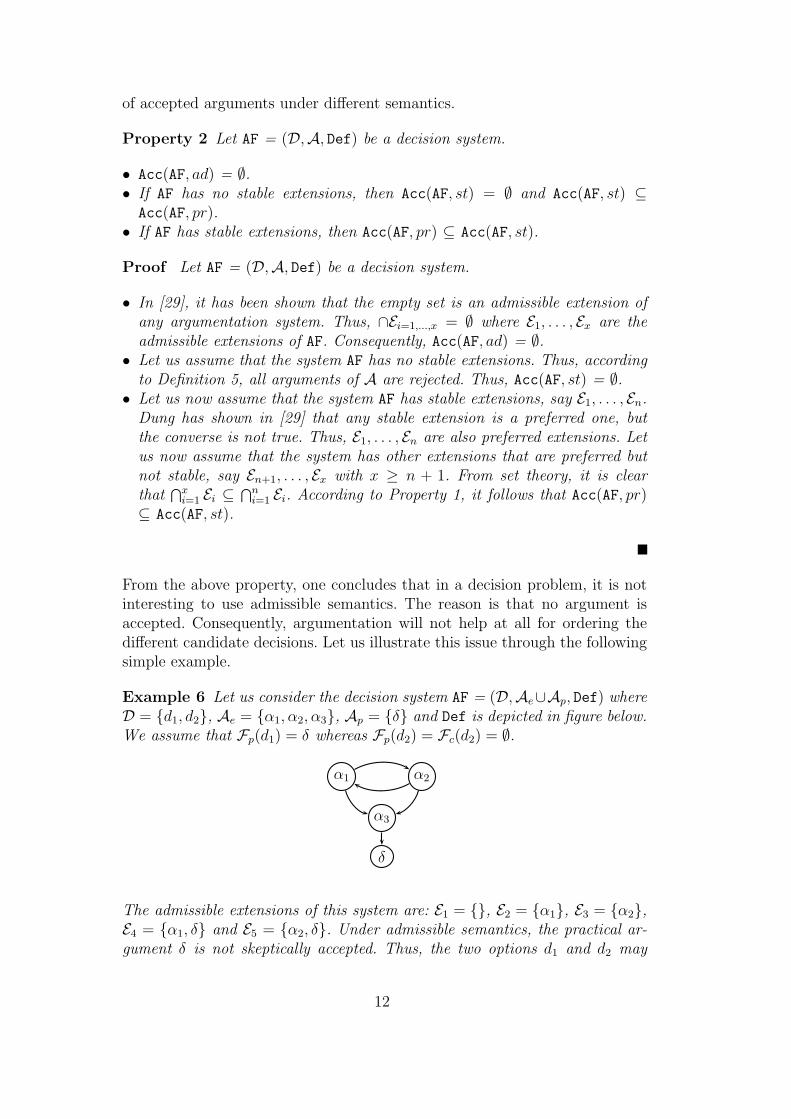
Example 6 Let us consider the decision system AF = (D,Ae∪Ap, Def) whereD = d1, d2, Ae = α1, α2, α3, Ap = δ and Def is depicted in figure below.We assume that Fp(d1) = δ whereas Fp(d2) = Fc(d2) = ∅.

α1 α2

α3

δ

The admissible extensions of this system are: E1 = , E2 = α1, E3 = α2,E4 = α1, δ and E5 = α2, δ. Under admissible semantics, the practical ar-gument δ is not skeptically accepted. Thus, the two options d1 and d2 may

12

be equally preferred since the first one has an argument but not an acceptedone, and the second has no argument at all. However, the same decision sys-tem has two preferred extensions: E4 and E5. Under preferred semantics, theset Acc(AF, pr) contains the argument δ (i.e. Acc(AF, pr) = δ). Thus, it isnatural to prefer the option d1 to d2.

Consequently, in the following, we will use stable semantics if the systemhas stable extensions, otherwise preferred semantics will be considered forcomputing the set Acc(AF, y).

Since the defeat relation Defp is empty, it is trivial that the practical systemAFp has exactly one preferred/stable extension which is the set Ap itself.

Property 3 The practical system AFp = (Ap, Defp) has a unique preferred/stableextension, which is the set Ap.

Proof This follows directly from the fact that the set Ap is conflict-free sinceDefp = ∅.

It is important to notice that the epistemic system AFe in its side is verygeneral and does not necessarily present particular properties like for instancethe existence of stable/preferred extensions.

In what follows, we will show that the result of the decision system dependsbroadly on the outcome of its epistemic system. The first result states thatthe epistemic arguments of each admissible extension of AF constitute an ad-missible extension of the epistemic system AFe.

Theorem 1 Let AF = (D,Ae ∪ Ap, Defe ∪ Defp ∪ Defm) be a decision sys-tem, E1, . . . , En its admissible extensions, and AFe = (Ae, Defe) its associatedepistemic system.

• ∀Ei, the set Ei ∩ Ae is an admissible extension of AFe.• ∀E ′ such that E ′ is an admissible extension of AFe, ∃Ei such that E ′ ⊆ Ei∩Ae.

Proof• Let Ei be an admissible extension of AF. Let E = Ei∩Ae. Let us assume thatE is not an admissible extension of AFe. There are two cases:Case 1: E is not conflict-free. This means that ∃α1, α2 ∈ E such that

(α1, α2) ∈ Defe. Thus, ∃α1, α2 ∈ Ei such that (α1, α2) ∈ Def. This isimpossible since Ei is an admissible extension, thus conflict-free.

Case 2: E does not defend its elements. This means that ∃α ∈ E, such that∃α′ ∈ Ae, (α′, α) ∈ Defe and ∄α′′ ∈ E such that (α′′, α′) ∈ Defe. Since(α′, α) ∈ Defe, this means that (α′, α) ∈ Def with α ∈ Ei. However, Ei isadmissible, then ∃a ∈ Ei such that (a, α′) ∈ Def. Assume that a ∈ Ap.This is impossible since practical arguments are not allowed to defeat

13

epistemic ones. Thus, a ∈ Ae. Hence, a ∈ E. Contradiction.• Let E ′ be an admissible extension of AFe. Let us prove that E ′ is an admissible

extension of AF. Assume that E ′ is not an admissible extension of AF. Thereare two possibilities: i) E ′ is not conflict-free in AF. This is not possible sinceE ′ an admissible extension of AFe, thus conflict-free.

ii) E ′ does not defend all its elements in the system AF. This means that∃a ∈ E ′ such that E ′ does not defend a. This means also that ∃b /∈ E ′

such that (b, a) ∈ Def and ∄c ∈ E ′ such that (c, b) ∈ Def. There are twocases: either b ∈ Ae or b ∈ Ap. b cannot be in Ae since E ′ is an admissibleextension thus defends its arguments against any attack, consequently itdefends also a against b. Assume now that b ∈ Ap, this is also impossiblesince practical arguments are not allowed to attack epistemic ones. Thus, E ′

is an admissible extension of the system AF.

Note that the above theorem holds as well for stable and preferred extensionssince each stable (resp. preferred) extension is an admissible one.

It is easy to show that when Defm is empty, i.e. no epistemic argument defeatsa practical one, then the extensions of AF (under a given semantics) are exactlythe different extensions of AFe (under the same semantics) augmented by theset AFp.

Theorem 2 Let AF = (D,Ae ∪Ap, Defe ∪ Defp ∪ Defm) be a decision system.Let E1, . . . , En be the extensions of AFe under a given semantics. If Defm = ∅then ∀Ei with i = 1, . . . , n, then the set Ei ∪ Ap is an extension of AF.

Proof Let E be an admissible extension of AFe. Let us assume that E ∪Ap isnot an admissible extension of AF. There are two cases:

Case 1: E ∪ Ap is not conflict-free. Since E and Ap are conflict-free, then∃α ∈ E and ∃δ ∈ Ap such that (α, δ) ∈ Def. Contradiction with the factthat Defm = ∅.

Case 2: E ∪ Ap does not defend its elements. This means that: i) ∃α ∈ Esuch that ∃α′ ∈ Ae, (α′, α) ∈ Defe and E ∪Ap does not defend it. Impossiblesince E is an admissible extension then it defends its arguments. ii) ∃δ ∈ Ap

such that ∃a ∈ A, and (a, δ) ∈ Def and δ is not defended by E ∪ Ap. SinceDefm = ∅ then a ∈ Ap. This is impossible since Rp = ∅. Contradiction.

Finally, it can be shown that if the empty set is the only admissible extensionof the decision system AF, then the empty set is also the only admissibleextension of the corresponding epistemic system AFe. Moreover, each practicalargument is attacked by at least one epistemic argument.

14

Theorem 3 Let AF = (D,Ae ∪Ap, Defe ∪ Defp ∪ Defm) be a decision system.The only admissible extension of AF is the empty set iff:

(1) The only admissible extension of AFe is the empty set, and(2) ∀δ ∈ Ap, ∃α ∈ Ae such that (α, δ) ∈ Defm.

Proof Let AF = (D,Ae ∪ Ap, Defe ∪ Defp ∪ Defm) be a decision system.

Case 1: Assume that the empty set is the only admissible extension of AF.Assume also that the epistemic system AFe has a non-empty admissible ex-tension,say E. This means that E is not an admissible extension of AF.There are two cases:a) E is not conflict-free. This is impossible since E is an admissible exten-sion of AFe.b) E does not defend its elements. This means that ∃a ∈ Ae ∪Ap such that∃b ∈ E and (a, b) ∈ Def and ∄c ∈ E such that (c, a) ∈ Def. There are twopossibilities: i) a ∈ Ap. This is impossible since practical arguments are notallowed to attack epistemic arguments. ii) a ∈ Ae. Since E is an admissibleextension of AFe, then ∃c ∈ E such that (c, a) ∈ Defe. Thus, (c, a) ∈ Def.Contradiction.

Case 2: Let us now assume that the empty set is the only admissible exten-sion of AFe and that ∀δ ∈ Ap, ∃α ∈ Ae such that (α, δ) ∈ Defm. Assumealso that ∃E 6= ∅ such that E is an admissible extension of the decisionsystem AF.

From Theorem 1, E ∩ Ae is an admissible extension of AFe. Since theonly admissible extension of AFe is the empty set, then E ∩ Ae = ∅. Thus,E ⊆ Ap.

Let δ ∈ E. By assumption, ∃α ∈ Ae such that (α, δ) ∈ Defm. Since Eis an admissible extension, thus it defends all its elements. Consequently,∃δ′ ∈ E such that (δ′, α) ∈ Def. Since E ⊆ Ap, then δ′ ∈ Ap. It is impossibleto have (δ′, α) ∈ Def since practical arguments are not allowed to attackepistemic ones.

At this step, we have only defined the accepted arguments among all theexisting ones. However, nothing is yet said about which option to prefer. Inthe next section, we will study different ways of comparing pairs of options onthe basis of skeptically accepted practical arguments.

2.5 Ordering options

Comparing candidate decisions, i.e. defining a preference relation on the setD of options, is a key step in a decision process. In an argumentation-based

15

approach, the definition of this relation is based on the sets of “accepted”arguments pro or cons associated with candidate decisions. Thus, the input ofthis relation is no longer Ap, but the set Acc(AF, y) ∩ Ap, where Acc(AF, y) isthe set of skeptically accepted arguments of the decision system (D,A, Def)under stable or preferred semantics. In what follows, we will use the notationAcc(AF) for short.

Note that in a decision system, when the defeat relation Defm is empty, theepistemic arguments become useless for the decision problem, i.e. for orderingoptions. Thus, only the practical system AFp is needed.

Depending on what sets are considered and how they are handled, one canroughly distinguish between three categories of principles:

Unipolar principles: are those that only refer to either the arguments proor the arguments con.

Bipolar principles: are those that take into account both types of argu-ments at the same time.

Non-polar principles: are those where arguments pro and arguments cona given choice are aggregated into a unique meta-argument. It results thatthe negative and positive polarities disappear in the aggregation.

Whatever the category is, a relation should suitably satisfy the followingminimal requirements:

(1) Transitivity: The relation should be transitive (as usually required indecision theory).

(2) Completeness: Since one looks for the “best” candidate decision, itshould then be possible to compare any pair of choices. Thus, the relationshould be complete.

2.5.1 Unipolar principles

In this section we present basic principles for comparing decisions on the basisof only arguments pro. Similar ideas apply to arguments con. We start bypresenting those principles that do not involve the strength of arguments,then their respective refinements when strength is taken into account.

A first natural criterion consists of preferring the decision that has more ar-guments pro.

Definition 6 (Counting arguments pro) Let AF = (D,A, Def) be a deci-sion system and Acc(AF) its accepted arguments. Let d1, d2 ∈ D.

d1 d2 iff |Fp(d1) ∩ Acc(AF)| ≥ |Fp(d2) ∩ Acc(AF)|.

16

Property 4 This relation is a complete preorder.

Note that when the decision system has no accepted arguments (i.e. Acc(AF) =∅), all the options in D are equally preferred w.r.t. the relation . It can bechecked that if a practical argument is defined as done later in Definition18, then with such a principle, one may prefer a decision d, which has threearguments pointing all to the same goal, to decision d′, which is supported bytwo arguments pointing to different goals.

When the strength of arguments is taken into account in the decision process,one may think of preferring a choice that has a dominant argument, i.e. anargument pro that is preferred w.r.t. the relation ≥p⊆ Ap×Ap to any argumentpro the other choices. This principle is called promotion focus principle in [3].

Definition 7 Let AF = (D,A, Def) be a decision system and Acc(AF) its ac-cepted arguments. Let d1, d2 ∈ D.

d1 d2 iff ∃δ ∈ Fp(d1) ∩ Acc(AF) such that ∀δ′ ∈ Fp(d2) ∩ Acc(AF), δ ≥p δ′.

With this criterion, if the decision system has no accepted arguments, thenall the options in D are equally preferred. The above definition relies heavilyon the relation ≥p that compares practical arguments. Thus, the propertiesof this criterion depend on those of ≥p. Namely, it can be checked that theabove criterion works properly if ≥p is a complete preorder.

Property 5 If the relation ≥p is a complete preorder, then is also a com-plete preorder.

Note that the above relation may be found to be too restrictive, since whenthe strongest arguments in favor of d1 and d2 have equivalent strengths (i.e.are indifferent), d1 and d2 are also seen as equivalent. However, we can refinethe above definition by ignoring the strongest arguments with equal strengths,by means of the following strict preorder.

Definition 8 Let AF = (D,A, Def) be a decision system and Acc(AF) its ac-cepted arguments. Let d1, d2 ∈ D, and ≥p be a complete preorder. Let (δ1,. . ., δr), (δ′1, . . ., δ′s) such that ∀δi=1,...,r, δi ∈ Fp(d1) ∩ Acc(AF), and ∀δ′j=1,...,s,δ′j ∈ Fp(d2) ∩ Acc(AF).

Each of these vectors is assumed to be decreasingly ordered w.r.t ≥p (e.g. δ1

≥p . . . ≥p δr). Let v = min(r, s).

d1 d2 iff:

• δ1 >p δ′1, or

17

• ∃ k ≤ v such that δk >p δ′k and ∀ j < k, δj ≈p δ′j, or• r > v and ∀ j ≤ v, δj ≈p δ′j.

Till now, we have only discussed decision principles based on arguments pro.However, the counterpart principles when arguments con are considered canalso be defined. Thus, the counterpart principle of the one defined in Definition6 is the following complete preorder:

Definition 9 (Counting arguments con) Let AF = (D,A, Def) be a deci-sion system and Acc(AF) its accepted arguments. Let d1, d2 ∈ D.

d1 d2 iff |Fc(d1) ∩ Acc(AF)| ≤ |Fc(d2) ∩ Acc(AF)|.

The principles that take into account the strengths of arguments have alsotheir counterparts when handling arguments con. The prevention focus prin-ciple prefers a decision when all its cons are weaker than at least one argumentagainst the other decision. Formally:

Definition 10 Let AF = (D,A, Def) be a decision system and Acc(AF) itsaccepted arguments. Let d1, d2 ∈ D.

d1 d2 iff ∃δ ∈ Fc(d2) ∩ Acc(AF) such that ∀δ′ ∈ Fc(d1) ∩ Acc(AF), δ ≥p δ′.

As in the case of arguments pro, when the relation ≥p is a complete preorder,the above relation is also a complete preorder, and can be refined into thefollowing strict one.

Definition 11 Let AF = (D,A, Def) be a decision system and Acc(AF) itsaccepted arguments. Let d1, d2 ∈ D.

Let (δ1, . . ., δr), (δ′1, . . ., δ′s) such that ∀δi=1,...,r, δi ∈ Fc(d1) ∩ Acc(AF), and∀δ′j=1,...,s, δ′j ∈ Fc(d2) ∩ Acc(AF).

Each of these vectors is assumed to be decreasingly ordered w.r.t ≥p (e.g. δ1

≥p . . . ≥p δr). Let v = min(r, s).d1 ≻ d2 iff:

• δ′1 >p δ1, or• ∃ k ≤ v such that δ′k >p δk and ∀ j < k, δj ≈p δ′j, or• v < s and ∀ j ≤ v, δj ≈p δ′j.

2.5.2 Bipolar principles

Let’s now define some principles where both types of arguments (pros andcons) are taken into account when comparing decisions. Generally speaking,

18

we can conjunctively combine the principles dealing with arguments pro withtheir counterpart handling arguments con. For instance, the principles givenin Definition 6 and Definition 9 can be combined as follows:

Definition 12 Let AF = (D,A, Def) be a decision system and Acc(AF) itsaccepted arguments. Let d1, d2 ∈ D. d1 d2 iff

• |Fp(d1) ∩ Acc(AF)| ≥ |Fp(d2) ∩ Acc(AF)|, and• |Fc(d1) ∩ Acc(AF)| ≤ |Fc(d2) ∩ Acc(AF)|.

However, note that unfortunately this is no longer a complete preorder. Sim-ilarly, the principles given respectively in Definition 7 and Definition 10 canbe combined into the following one:

Definition 13 Let AF = (D,A, Def) be a decision system and Acc(AF) itsaccepted arguments. Let d1, d2 ∈ D. d1 d2 iff:

• ∃ δ ∈ Fp(d1) ∩ Acc(AF) such that ∀ δ′ ∈ Fp(d2) ∩ Acc(AF), δ ≥p δ′, and• ∄ δ ∈ Fc(d1) ∩ Acc(AF) such that ∀ δ′ ∈ Fc(d2) ∩ Acc(AF), δ ≥p δ′.

This means that one prefers a decision that has at least one supporting argu-ment which is better than any supporting argument of the other decision, andalso has not a very strong argument against it. Note that the above definitioncan be also refined in the same spirit as Definitions 8 and 11.

Another family of bipolar decision principles applies the Franklin principlewhich is a natural extension to the bipolar case of the idea underlying Defi-nition 8. This principle consists, when comparing pros and cons a decision, ofignoring pairs of arguments pro and cons which have the same strength. Aftersuch a simplification, one can apply any of the above bipolar principles. Inwhat follows, we will define formally the Franklin simplification.

Definition 14 (Franklin simplification) Let AF = (D,A, Def) be a deci-sion system and Acc(AF) its accepted arguments. Let d ∈ D.

Let P = (δ1, . . ., δr), C = (δ′1, . . ., δ′m) such that ∀δi, δi ∈ Fp(d) ∩ Acc(AF)and ∀δ′j, δ

′j ∈ Fc(d) ∩ Acc(AF).

Each of these vectors is assumed to be decreasingly ordered w.r.t ≥p (e.g. δ1

≥p . . . ≥p δr). The result of the simplification is P ′ = (δj+1, . . ., δr), C ′ =(δ′j+1, . . ., δ′m) s.t.

• ∀ 1 ≤ i ≤ j, δi ≈p δ′i and (δj+1 >p δ′j+1 or δ′j+1 >p δj+1)• If j = r (resp. j = m), then P ′ = ∅ (resp. C ′ = ∅).

19

2.5.3 Non-polar principles

In some applications, the arguments in favor of and against a decision are ag-gregated into a unique meta-argument having a unique strength. Thus, com-paring two decisions amounts to compare the resulting meta-arguments. Sucha view is well in agreement with current practice in multiple criteria decisionmaking, where each decision is evaluated according to different criteria us-ing the same scale (with a positive and a negative part), and an aggregationfunction is used to obtain a global evaluation of each decision.

Definition 15 (Aggregation criterion) Let AF = (D,A, Def) be a decisionsystem and Acc(AF) its accepted arguments. Let d1, d2 ∈ D. Let (δ1, . . ., δn) 4

and (δ′1, . . ., δ′m) 5 (resp. (γ1, . . . , γl)6 and (γ′

1, . . . , γ′k)

7 ) the vectors of thearguments pro and cons the decision d1 (resp. d2).d1 d2 iff h(δ1, . . ., δn, δ′1, . . ., δ′m) ≥p h(γ1, . . ., γl, γ′

1, . . ., γ′k), where h is

an aggregation function.

A simple example of this aggregation attitude is computing the difference ofthe number of arguments pros and cons.

Definition 16 Let AF = (D,A, Def) be a decision system and Acc(AF) itsaccepted arguments. Let d1, d2 ∈ D. d1 d2 iff |Fp(d1)∩ Acc(AF)| − |Fc(d1)∩Acc(AF)| ≥ |Fp(d2) ∩ Acc(AF)| − |Fc(d2) ∩ Acc(AF)|.

This has the advantage to be again a complete preorder, while taking intoaccount both pros and cons arguments.

3 A typology of formal practical arguments

This section aims at presenting a systematic study of practical arguments.Epistemic arguments will not be discussed here because they have been muchstudied in the literature (eg. [4,14,46]), and their handling does not makenew problems in the general setting of Section 2, even in the decision processperspective of this paper. Moreover, they only play a role when the knowl-edge base is inconsistent. Before presenting the different types of practicalarguments, we start first by introducing the logical language as well as thedifferent bases needed in a decision making problem.

4 Each δi ∈ Fp(d1) ∩ Acc(AF).5 Each δ′i ∈ Fc(d1) ∩ Acc(AF).6 Each γi ∈ Fp(d2) ∩ Acc(AF).7 Each γ′

i ∈ Fc(d2) ∩ Acc(AF).

20

3.1 Logical representation of knowledge and preference

This section introduces the representation setting of knowledge and preferencewhich are here distinct, as it is in classical decision theory. Moreover, prefer-ences are supposed to be handled in a bipolar way, which means that whatthe decision maker is really looking for may be more restrictive than what itis just willing to avoid.

In what follows, a vocabulary P of propositional variables contains two kindsof variables: decision variables, denoted by v1, . . . , vn, and state variables. De-cision variable are controllable, that is their value can be fixed by the decisionmaker. Making a decision then amounts to fixing the truth value of every de-cision variable. On the contrary, state variables are fixed by nature, and theirvalue is a matter of knowledge by the decision maker. He has no control onthem (although he may express preferences about their values).

(1) D is a set of formulas built from the decision variables. Elements of Drepresent the different alternatives, or candidate decisions. Let us considerthe following example of an agent who wants to know whether she shouldtake her umbrella, her raincoat or both. In this case, there are two decisionvariables: umb (for umbrella) and rac (for raincoat). Assume that thisagent hesitates between the three following options: i) d1 : umb (i.e. totake her umbrella), ii) d2 : rac (i.e. to take her raincoat), or iii) d3 :umb∧ rac (i.e. to take both). Thus, D = d1, d2, d3. Note that elementsof D are not necessarily mutually exclusive. In the example, if the agentchooses the option d3 then the two other options are satisfied.

(2) G is a set of propositional formulas built from state variables. It gathersthe goals of an agent (the decision maker). A goal represents what theagent wants to achieve, and has thus a positive flavor. This means thatif g ∈ G, the decision maker wants that the chosen decision leads to astate of affairs where g is true. This base may be inconsistent. In thiscase it would be for sure impossible to satisfy all the goals, which wouldinduce the simultaneous existence of practical arguments pro and cons. Ingeneral G contains several goals. Clearly, an agent should try to satisfy allgoals in its goal base G if possible. This means that G may be thought as aconjunction. However, the two goal bases G = g1, g2 and G ′ = g1 ∧ g2although they are logically equivalent, will not be handled in the sameway in an argumentative perspective, since in the second case there isno way to consider intermediary objectives such as here satisfying g1,or satisfying g2 only, in case it turns out that it is impossible to satisfyg1 ∧ g2. This means that our approach is syntax-dependent.

(3) The set R is a set of propositional formulas built from state variables. It

21

gathers the rejections of an agent. A rejection represents what the agentwants to avoid. Clearly rejections express negative preferences. The set¬r|r ∈ R describing what is acceptable for the agent is assumed tobe consistent, since acceptable alternatives should satisfy ¬r due to therejection of r, and at least there should remain some possible worlds thatare not rejected. There are at least two reasons for separately consideringa set of goals and a set of rejections. First, since agents naturally expressthemselves in terms of what they are looking for (i.e. their goals), andin terms of what they want to avoid (i.e. their rejections), it is better toconsider goals and rejections separately in order to articulate argumentsreferring to them in a way easily understandable for the agents. Moreover,recent cognitive psychology studies [18] have confirmed the cognitive va-lidity of this distinction between goals and rejections. Second, if r is arejection, this does not necessarily mean that ¬r is a goal, and thus re-jections cannot be equivalently restated as goals. For instance, in case ofchoosing a medical drug, one may have as a goal the immediate availabil-ity of the drug, and as a rejection its availability only after at least twodays. In such a case, if the candidate decision guarantees the availabilityonly after one day, this decision will for sure avoid the rejection withoutsatisfying the goal. Another simple example is the case of an agent whowants to get a cup of either coffee or tea, and wants to avoid gettingno drink. If the agent obtains a glass of water, again he would avoid itsrejection, without being completely satisfied.We can imagine different forms of consistency between the goals and therejections. A minimal requirement is to have G ∩R = ∅, otherwise it willmean that an agent both wants to have p true and to avoid it.

(4) The set K represents the background knowledge that is not necessarilyassumed to be consistent. The argumentation framework for inferencepresented in Section 2 will handle such inconsistency, namely with theepistemic system. Elements of K are propositional formulas built fromthe alphabet P , and assumed to be put in a clausal form. The base Kcontains basically two kinds of clauses: i) those not involving any elementfrom D, which encode pieces of knowledge or factual information (possiblyinvolving goals) about how the world is; ii) those involving one negationof a formula d of the set D, and which states what follows when decisiond is applied.

Thus, the decision problem we consider will always be encoded with the fourabove sets of formulas (with the restrictions stated above). Moreover, we sup-pose that each of the three bases K, G, and R are stratified. Having K stratifiedwould mean that we consider that some pieces of knowledge are fully certain,while others are less certain (maybe distinguishing between several levels ofpartial certainty such as “almost certain”, “rather certain”, ...). Clearly, for-mulas that are not certain at all cannot be in K. Similarly, having G (resp. R)

22

stratified means that some goals (resp. rejections) are imperative, while someothers are less important (one may have more than two levels of importance).Completely unimportant goals (resp. rejections) do not appear in any stratumof G (resp. R).

It is worth pointing out that we assume that candidate decisions are all con-sidered as a priori equally potentially suitable, and thus there is no need tohave D stratified.

For encoding the stratifications, we use the set 0, 1,. . . , n of integers as a lin-early ordered scale, where n stands for the highest level of certainty if dealingwith K (resp. level of importance if dealing with G or R) and ‘0’ correspondsto the complete lack of certainty (resp. importance). Other encodings (e.g.using levels inside the unit interval or using the integer scale in a reversedway) would be equivalent.

Definition 17 (Decision theory) A decision theory (or a theory for short)is a tuple T = 〈D, K, G, R〉.

• The base K is partitioned and stratified into K1, . . ., Kn (K = K1 ∪ . . . ∪Kn) such that formulas in Ki have the same certainty level and are morecertain than formulas in Kj where j < i. Moreover, K0 is not consideredsince it gathers formulas which are completely uncertain.

• The base G is partitioned and stratified into G1, . . ., Gn (G = G1 ∪ . . . ∪Gn) such that goals in Gi have the same importance and are more importantthan goals in Gj where j < i. Moreover, G0 is not considered since it gathersgoals which are completely unimportant.

• The base R is partitioned and stratified into R1, . . ., Rn (R = R1 ∪ . . .∪ Rn) such that rejections in Ri have the same importance and are moreimportant than rejections in Rj where j < i. Moreover, R0 is not consideredsince it gathers rejections which are completely unimportant.

3.2 A typology of formal practical arguments

Each candidate decision may have arguments in its favor (called pros), andarguments against it (called cons). In the following, an argument is associatedwith an alternative, and always either refers to a goal or to a rejection.

Arguments pros point out the “existence of good consequences” or the “ab-sence of bad consequences” for a candidate decision. A good consequencemeans that applying decision d will lead to the satisfaction of a goal, or tothe avoidance of a rejection. Similarly, a bad consequence means that theapplication of d leads for sure to miss a goal, or to reach a rejected situation.

23

We can distinguish between practical arguments referring to a goal, and thosearguments referring to rejections. When focusing on the base G, an argumentpro corresponds to the guaranteed satisfaction of a goal when there exists aconsistent subset S of K such that S ∪ d ⊢ g.

Definition 18 (Positive arguments pro) Let T be a theory. A positivelyexpressed argument in favor of an option d is a tuple δ = 〈S, d, g〉 s.t:

(1) S ⊆ K, d ∈ D, g ∈ G, S ∪ d is consistent(2) S ∪ d ⊢ g, and S is minimal for set inclusion among subsets of K

satisfying the above criteria (arguments of Type PP).

S is called the support of the argument, and d is its conclusion. Let APP bethe set of all arguments of type PP that can be built from a decision theory T .

In what follows, Supp denotes a function that returns the support S of anargument, Conc denotes a function that returns the conclusion d of the ar-gument, and Result denotes a function that returns the consequence of thedecision. The consequence may be either a goal as in the previous definition,or a rejection as we can see in the next definitions of argument types.

The above definition deserves several comments.

• The consistency of S ∪ d means that d is applicable in the context S, inother words that we cannot prove from S that d is impossible. This meansthat impossible alternatives w.r.t. K have been already taken out whendefining the set D. In the particular case where the base K would be consis-tent, then condition 1, namely S∪d is consistent, is equivalent to K∪dis consistent. But, in the case where K is inconsistent, independently fromthe existence of a PP argument, it may happen that for another consistentsubset S ′ of K, S ′ ⊢ ¬d. This would mean that there is some doubt aboutthe feasibility of d, and then constitute an epistemic argument against d. Inthe general framework proposed in section 2, such an argument will overruledecision d since epistemic arguments take precedence over any practical ar-gument (provided that this epistemic argument is not itself killed by anotherepistemic argument).

• Note that argument of type PP are reminiscent of the practical syllogismrecalled in the introduction. Indeed, it emphasizes that a candidate deci-sion might be chosen if it leads to the satisfaction of a goal. However, thisis only a clue for choosing the decision since this last may have argumentsagainst, which would weaken it, or there may exist other candidate deci-sions with stronger arguments. Moreover, due to the nature of the practicalsyllogism, it is worth noticing that practical arguments have an abductiveform, contrarily to epistemic arguments that are defined in a deductive way,as revealed by their formal respective definitions.

24

Another type of arguments pro refers to rejections. It amounts to avoid arejection for sure, i.e. S ∪ d ⊢ ¬r (where S is a consistent subset of K).

Definition 19 (Negative arguments pro) Let T be a theory. A negativelyexpressed argument in favor of an option is a tuple δ = 〈S, d, r〉 s.t:

(1) S ⊆ K, d ∈ D, r ∈ R, S ∪ d is consistent(2) S ∪ d ⊢ ¬r and S is minimal for set inclusion among subsets of K

satisfying the above criteria (arguments of Type NP).

Let ANP be the set of all arguments of type NP that can be built from a decisiontheory T .

Arguments cons highlight the existence of bad consequences for a given can-didate decision. Negatively expressed arguments con are defined by exhibitinga rejection that is necessarily satisfied. Formally:

Definition 20 (Negative arguments con) Let T be a theory. A negativelyexpressed argument against an option d is a tuple δ = 〈S, d, r〉 s.t:

(1) S ⊆ K, d ∈ D, r ∈ R, S ∪ d is consistent,(2) S ∪ d ⊢ r and S is minimal for set inclusion among subsets of K

satisfying the above criteria (arguments of Type NC).

Let ANC be the set of all arguments of type NC that can be built from a decisiontheory T .

Lastly, the absence of positive consequences can also be seen as an argumentagainst (cons) an alternative.

Definition 21 (Positive arguments con) Let T be a theory. A positivelyexpressed argument against an option d is a tuple δ = 〈S, d, g〉 s.t:

(1) S ⊆ K, d ∈ D, g ∈ G, S ∪ d is consistent,(2) S ∪ d ⊢ ¬g and S is minimal for set inclusion among subsets of K

satisfying the above criteria (arguments of Type PC).

Let APC be the set of all arguments of type PC that can be built from a decisiontheory T .

Let us illustrate the previous definitions on an example.

Example 7 Two decisions are possible, organizing a show (d), or not (¬d).Thus D = d,¬d. The knowledge base K contains the following pieces ofknowledge: if a show is organized and it rains then small money loss (¬d ∨¬r∨ sml); if a show is organized and it does not rain then benefit (¬d∨ r∨ b);small money loss entails money loss (¬sml∨ml); if benefit there is no money

25

loss (¬b∨¬ml); small money loss is not large money loss (¬sml∨¬lml); largemoney loss is money loss (¬lml∨ml); there are clouds (c); if there are cloudsthen it may rain (¬c ∨ r). All these pieces of knowledge are in the stratumof level n, except the last one which is in a stratum with a lower level dueto uncertainty. Consider now the cases of two organizers (O1 and O2) havingdifferent preferences. O1 does not want any loss R = ml, and would likebenefit G = b. O2 does not want large money loss R = lml, and wouldlike benefit G = b. In such case, it is expected that O1 prefers ¬d to d, sincethere is a NC argument against d and no argument for ¬d. For O2, there isno longer any NC argument against d. He might even prefer d to ¬d, if heis optimistic and he considers that there is a possibility that it does not rain(leading to a potential PP argument under the hypothesis to have ¬r in K.

Due to the asymmetry in human mind between what is rejected and what isdesired, the former being usually considered as stronger than the latter, onemay assume that NC arguments are stronger than PC arguments, and converselyPP arguments are stronger than NP arguments.

In classical decision frameworks, bipolarity is not considered. Indeed, we arein the particular case where rejections mirror goals in the sense that g is agoal iff ¬g is a rejection. Consequently, in our argumentation setting the twotypes NC and PC coincide. Similarly, the two types PP and NP are the same.

4 Application to multiple criteria decision making

4.1 Introduction to multiple criteria decision making

In multiple criteria decision making, each candidate decision d in D is eval-uated from a set C of m different points of view (i = 1,m), called criteria.The evaluation can be done in an absolute manner or in a relative way. Thismeans that for each i, d can be either evaluated by an absolute estimate Ci(d)belonging to the evaluation scale used for i, or there exists a valued preferencerelation Ri(d, d′) associated with each i that is applicable to any pair (d, d′) ofelements of D. Then one can distinguish between two families of approaches:i) the ones based on a global aggregation of value criteria-based functionswhere the obtained global absolute evaluations are of the form g(f1(C1(d), . . .,fm(Cm(d))) where the mappings fi map the original evaluations on a uniquescale, which assumes commensurability, and ii) the ones that aggregate thepreference indices Ri(d, d′) into a global preference R(d, d′) from which a rank-ing of the elements in D can be obtained. In the following, only the first typeof approach is considered.

26

4.2 Arguments in multiple criteria decision making

The decision maker uses a set C of different criteria. For each criterion ci,one assumes that we have a bipolar univariate ordered scale Ti which enablesus to distinguish between positive and negative values. Such a scale has aneutral point, or more generally a neutral area that separates positive andnegative values. The lower bound of the scale stands for total dissatisfactionand the upper bound for total satisfaction, while neutral value(s) stand forindifference. The closer to the upper bound the value of criterion ci for choiced, denoted ci(d) is, the more satisfactory choice d is w.r.t ci; the closer to thelower bound the value of criterion ci for choice d is, the more dissatisfactorychoice d is w.r.t ci. As in multiple criteria aggregation, we assume that thedifferent scales Ti can be mapped on a unique bipolar scale T , i.e. for any i,fi(ci(d)) ∈ T . Moreover, we assume here that T is discrete and will be denotedT = −k, . . ., −1, 0, +1, . . ., +k with the classical ordering convention ofrelative integers.

Example 8 (Choosing an apartment) Imagine we have a set C of threecriteria for choosing an apartment: Price (c1), Size (c2), and Location w.r.t.downtown (c3). The criteria are valued on the same bipolar univariate scale−2,−1, 0, +1, +2 (this means that all the fi mappings are the identity).Prices of apartments may be judged ’very expensive’, ’expensive’, ’reason-ably priced’, ’cheap’, ’very cheap’. Size may be ’very small’, ’small’, ’nor-mal sized’, ’large’, ’very large’. Distance may be ’very far’, ’far’, ’medium’,’close’, ’very close’. In each case, the five linguistic expressions would be val-ued by −2,−1, 0, +1, +2 respectively. Thus an apartment d that is expensive,medium-sized, and very close to downtown will be evaluated as c1(d) = −1,c2(d) = 0, and c3(d) = +2. It is clear that this scale implicitly encodes thatthe best apartments are those that are very cheap, very large, and very closeto both downtown and transportation.

From this setting, it is possible to express goals and rejections in terms ofcriteria values. A bipolar-valued criterion can be straightforwardly translatedinto a set of stratified goals, and a stratified set of rejections. The idea isthe following. The criteria may be satisfied either in a positive way (if thesatisfaction degree is higher than the neutral point 0 of T ) or in a negativeway (if the satisfaction degree is lower than the neutral point of T ). Formallyspeaking, the two bases G and R are defined as follows: having the conditionfi(ci(d)) ≥ +j satisfied, where +j belongs to the positive part of T , is a goalgj for the agent that uses ci as a criterion. This goal is all the more importantas j is small (but positive), since as suggested by the above example, theless restrictive conditions are the most imperative ones. The importance ofgj can be taken as equal to k − j + 1 for j ≥ 1 (using the standard order-reversing map on 1, ..., k). Indeed the most important condition fi(ci(d))

27

≥ +1 will have the maximal value in T , while the condition fi(ci(d)) ≥ +kwill have the minimal positive level in T , i.e. +1. We can proceed similarlywith rejections. The rejection rj corresponding to the condition fi(ci(d)) ≤ −jwill have importance j (importance uses only the positive part of the scale).This corresponds to the view of a fuzzy set as a nested family of level cuts,which translates in possibilistic logic into a collection of propositions whoseextensions are all the larger as the proposition is more imperative. In the aboveexample, consider for instance the price criterion. We will have two goals: g1 =very cheap and g2 = cheap with respective weights 1 and 2. Thus, being cheapis more imperative than being very cheap as expected. Similarly, r1 = veryexpensive and r2 = expensive are rejections with respective weights 2 and 1.Note that if an apartment is normally sized, then there will be no argumentin favor or against it w.r.t. its size.

In multiple criteria aggregation, criteria may have different levels of impor-tance. Let wi ∈ 0, +1, . . ., +k be the importance of criterion ci. Then, wecan apply the above translation procedure where, now the importance k−j+1of condition fi(ci(d)) ≥ +j is changed into min(wi, k − j + 1). Indeed, if wi ismaximal, i.e. wi = +k, the importance is unchanged; in case the importancewi of criterion ci would be minimal, i.e. wi = 0, then the resulting importanceof the associated goal (the condition fi(ci(d)) ≥ +j) is indeed also 0 expressingits complete lack of importance.

In addition to the bases D, C, G and R, the decision maker is also equippedwith a stratified knowledge base K encoding what he knows. In particular, Kcontains factual information about the values of the fi(ci(x))’s for the differentcriteria and the different candidate decisions. K also contains rules expressingthat values in T are linearly ordered, i.e. rules of the form if ci(x) ≥ j, thenci(x) ≥ j′ if j ≥ j′ ∈ T . More generally, K can also contain pieces of knowledgethat enable the decision maker to evaluate criteria from more elementary eval-uation of facts. This may be useful in practice for describing complex notions,e.g. comfort of a house in our example, which indeed may depend on manyparameters. A goal is assumed to be associated with a unique criterion areno longer allowed). Then, a goal gj

i is associated to a criterion ci by a propo-sitional formula of the form gj

i → ci meaning just that the goal gji refers to

the evaluation of criterion ci. Such formulas will be added to Kn. Note that inclassical multiple criteria problems, complete information is usually assumedw.r.t. the precise evaluation of criteria. Clearly, our setting is more generalsince it leaves room to incomplete information, and facilitates the expressionof goals and rejections.

Now that the different bases are introduced, we can apply our general decisionsystem, and build the arguments pro and cons for any candidate decision. Inaddition to the completeness of information, it is usually assumed in classicalapproaches to multiple criteria decision making that knowledge is consistent.

28

In such a case, it is not possible to have conflicting evaluations of a criterionfor a choice. Consequently, the whole power of our argumentation setting willnot be used, in particular all arguments will be accepted.

4.3 Retrieving some classical multiple criteria aggregations

The aim of this subsection is to show the agreement of the argumentation-based approach with some classical approaches to multiple criteria decisionmaking. It is worth mentioning that until recently, most multiple criteria ap-proaches use only positive evaluations, i.e. unipolar scales ranging from “bad”to “good” values, rather than distinguishing genuinely good values from re-ally bad ones that have to be rejected. The argumentation-based approachmakes natural the reference to the distinction between what is favored andwhat is disfavored by the decision maker for giving birth to arguments for andarguments against candidate decisions. Here, only two types of arguments areneeded: positive arguments pro of type PP, and negative arguments con of typeNC since rejections in this case are just the complement of goals. Indeed, thenegative values of a criterion reflect the fact that we are below some thresholdwhile the positive values express to what extent we are above. Thus, Ap =APP ∪ ANC.

In what follows, the base K is supposed to be consistent, fully certain (i.e.K = Kn), and to contain complete information w.r.t. the evaluation of criteria.Thus, the set A of arguments is exactly Ae ∪ Ap. Since K is consistent, then thetwo attack relations Re and Rm are empty (i.e. Re = Rm = ∅). Consequently,Defe = Defm = ∅, and the set of skeptically accepted arguments of the decisionsystem AF = (D,A, Def = ∅) is exactly Acc(AF) = A.

The first category of classical approaches to multiple criteria decision makingthat we will study is the one that gives the same importance to the differentcriteria of the set C. The idea is to prefer the alternative that satisfies positivelymore criteria. Let c′i(d) = 1 if ci(d) > 0 and c′i(d) = 0 if ci(d) < 0, where ci(d)is the evaluation of choice d by the i-th criterion. In order to capture this idea,a particular unipolar principle is used. Before introducing this principle, letus first define a function Results that returns for a given set B of practicalarguments, all the consequences of those arguments, i.e. all the goals andrejections to which arguments of B refer to.

Definition 22 Let d1, d2 ∈ D. d1 d2 iff Results(Fp(d2)) ⊆ Results(Fp(d1)).

Note that in our case, Fp(d) ⊆ APP and Fc(d) ⊆ ANC for a given d ∈ D.

Property 6 Let AF = (D,A, Def) be a decision system. Let d1, d2 ∈ D. WhenC = Cn, d1 d2 (according to Definition 22) iff

∑i c

′i(d1) ≥

∑i c

′i(d2).

29

If we focus on arguments con, the idea is to prefer the option that violatesless criteria. Let c′′i (d) = 0 if ci(d) > 0 and c′′i (d) = 1 if ci(d) < 0. This idea iscaptured by the following unipolar principle.

Definition 23 Let d1, d2 ∈ D. d1 d2 iff Results(Fc(d1)) ⊆ Results(Fc(d2)).

Property 7 Let (D,A, Def) be a decision system. Let d1, d2 ∈ D. When C =Cn, d1 d2 (according to Definition 23) iff

∑i c

′′i (d1) ≤

∑i c

′′i (d2).

When the criteria do not have the same level of importance, the promotionfocus principle given in Definition 7 amounts to use maxi c′i(d) with c′i(d) =ci(d) if ci(d) > 0 and c′i(d) = 0 if ci(d) < 0 as an evaluation function forcomparing decisions. Recall that the promotion focus principle is based on apreference relation ≥p between arguments. In what follows, we will propose adefinition of the force of an argument, as well as a definition of ≥p. The twodefinitions are chosen in such a way that they will allow us to retrieve theabove idea on the promotion focus principle.

In our application, the force of an argument depends on two components: thecertainty level of the knowledge involved in the argument, and the importancedegree of the goal (or rejection). Formally:

Definition 24 (Force of an argument) Let δ = 〈S, d, g〉 ∈ APP (resp. δ =〈S, d, r〉 ∈ ANC). The strength of δ is a pair (Lev(δ), Wei(δ)) s.t.

• The certainty level of the argument is Lev(δ) = mini|1 ≤ i ≤ n such thatSi 6= ∅, where Si denotes S ∩ Ki. If S = ∅ then Lev(δ) = n.

• The weight of the argument is Wei(δ) = j if g ∈ Gj (resp. r ∈ Rj).

The levels of satisfaction of the criteria should be balanced with their relativeimportance. Indeed, for instance, a criterion ci highly satisfied by d is not astrong argument in favor of d if ci has little importance. Conversely, a poorlysatisfied criterion for d is a strong argument against d only if the criterion isreally important. Moreover, in case of uncertain criteria evaluation, one mayhave to discount arguments based on such evaluation. In other terms, the forceof an argument represents to what extent the decision will satisfy the mostimportant criteria. This suggests the use of a conjunctive combination of thecertainty level, the satisfaction / dissatisfaction degree and the importance ofthe criterion. This requires the commensurateness of the scales.

Definition 25 (Conjunctive strength) Let δ, δ′ ∈ APP.δ >p δ′ iff min(Lev(δ), Wei(δ)) > min(Lev(δ′), Wei(δ′)).

Property 8 Let AF = (D,A, Def) be a decision system. Let d1, d2 ∈ D. WhenC = Cn, d1 d2 (according to Definition 7 and using Definition 25 for therelation ≥p) iff maxi c′i(d1) ≥ maxi c′i(d2).

30

The prevention focus principle (see Definition 10) amounts to use mini c′′i (d)with c′′i (d) = 0 if ci(d) > 0 and c′′i (d) = −ci(d) if ci(d) < 0.

Property 9 Let AF = (D,A, Def) be a decision system. Let d1, d2 ∈ D. WhenC = Cn, d1 d2 (according to Definition 10 and using Definition 25 for therelation ≥p) iff mini c′′i (d1) ≤ mini c′′i (d2).

When each criterion ci is associated with a level of importance wi rangingon the positive part of the criteria scale, the above c′i(d) is changed intomin(c′i(d), wi) in the promotion case.

Property 10 Let AF = (D,A, Def) be a decision system. Let d1, d2 ∈ D. d1

d2 (according to Definition 7 and using Definition 25 for the relation ≥p)iff maxi min(c′i(d1), wi) ≥ maxi min(c′i(d2), wi).

This expresses that d is all the more preferred as there is an important cri-terion that is positively evaluated. A similar proposition holds for the pre-vention focus principle. Thus, weighted disjunctions and conjunctions definedin [27] are retrieved. It would even be possible to provide the argumenta-tive counter-part of a general qualitative weighted conjunction of the formminimax(ci(d), neg(wi)), where neg is the reversing map of the discrete scalewhere wi takes its value. However, this would be quite similar to the qualitativedecision making under uncertainty problem which is now discussed in greatdetail, and where aggregations having the same structure are encountered.

5 Application to decision making under uncertainty

Decision making under uncertainty relies on the comparative evaluation ofdifferent alternatives on the basis of a decision principle, which can be usu-ally justified by means of a set of rationality postulates. This is, for example,the Savage view of decision making under uncertainty based on expected util-ity [45]. Thus, standard approaches for making decisions under uncertaintyconsist in defining decision principles in terms of analytical expressions thatsummarize the whole decision process, and for which it is shown that theyencode a preference relation obeying postulates that are supposedly mean-ingful. Apart from quantitative principles such as expected utility, anotherexample of such an approach is provided by the qualitative pessimistic oroptimistic decision principles, which have been more recently proposed andalso axiomatically justified [28,35]. The qualitative nature of these decisionevaluations make them more liable to be unpacked in terms of arguments infavor/against each choice, in order to better understand the underpinnings ofthe evaluation. We successively study the pessimistic and optimistic decisionprinciples. Note, however, that these qualitative decision criteria do not make

31

use of a bipolar univariate scale, so in the following we apply our general deci-sion system with an empty set of rejections. Thus, we will consider a decisiontheory T = 〈D,K,G〉. Consequently, the set of practical arguments built fromsuch a theory is Ap = APP ∪ APC. Recall that arguments of type PP are protheir conclusions whereas arguments of type PC are cons their conclusions. Inclassical decision systems, the knowledge base and the goals base are assumedto be consistent. Thus, in what follows, we will assume that they are consis-tent as well. Thus, the three defeat relations Defe, Defp and Defm are empty.Consequently, the decision system that will be used is (D,Ae ∪ Ap, Def = ∅).In such a system, the whole decision process is reduced to the last step, whichconsists of ordering pairs of options. This means that in order to show howpessimistic and optimistic principles are captured, it is sufficient to choose themost suitable decision principle among the ones proposed in Section 2.5.

5.1 Pessimistic Criterion

The pessimistic decision criterion is defined as follows: given a possibility dis-tribution πd restricting the plausible states that can be reached when a deci-sion d takes place, and a qualitative utility function µ, the so-called pessimisticqualitative decision principle, which estimates a kind of qualitative expecta-tion, is defined as [28]:

E∗(d) = minω

max (µ(ω), neg(πd(ω))) (1)

where πd is a mapping from a set of interpretations Ω to a linearly orderedscale U = 0, 1, ..., n, and µ is a mapping from Ω to the same scale U , and negis the involutive order-reversing map on U = 0, 1, . . . , n such that neg(0) =n and and neg(n) = 0, where 0 and n are the bottom and the top elements ofU . Namely, neg(n − k) = k. Thus, πd(ω) (resp. µ(ω)) is all the greater as ωis more plausible (resp. satisfactory), 0 standing for the minimal level, and nfor the maximal level. Moreover, πd and µ are assumed to be normalized, i.e.∃ ω ∈ Ω such that πd(ω) = 1, and similarly ∃ ω′ ∈ Ω, µ(ω′) = 1.

E∗(d) is all the greater as all the states ω that have some plausibility accordingto πd are among the most preferred states according to µ. E∗(d) is in fact adegree of inclusion of the fuzzy set of plausible states (when d is applied)into the fuzzy set of preferred states. The pessimistic utility E∗(d) is small assoon as there exists a possible consequence of d that is both highly plausibleand has a low satisfaction level with respect to preferences. This is clearly arisk-averse and thus a pessimistic attitude.

32

In [26], it has been shown that a stratified knowledge base has a possibilitydistribution as semantic counterpart. See annex for a refresher on possibilisticlogic. Let Kd be the knowledge base built from the base K to which the decisiond is added to the stratum Kn. Let πd be the possibility distribution associatedwith Kd, and µ be the possibility distribution associated with the base G ofgoals. The normalization of πd and µ is equivalent to the non-emptiness ofthe highest strata Kn and Gn. It has been shown in [24] that it is possibleto compute E∗(d), as expressed by formula 1, by only using a classical logicmachinery on x-level cuts of the two bases Kd and G.

Proposition 1 [24] E∗(d) is the maximal value of x ∈ U s.t.

(Kd)x ⊢ (G)neg(x) (2)

where (B)x (resp. (B)x) is the set of formulas of a base B that appear in thestrata x, . . . , n (resp. in the strata x + 1, . . . , n). Mind that (B)x is a set ofstrata, while Bx is a stratum. By convention, E∗(d) = 0 if there is no such x.

E∗(d) is equal to n (x = n) if the completely certain part of Kd entails thesatisfaction of all the goals, even the ones with low priorities.

In the pessimistic view, as pointed out by Proposition 1, we are interested infinding a decision d (if it exists) such that Kx ∪ d ⊢ Gy with x high andy low, i.e. such that the decision d together with the most certain part of Kentails the satisfaction of the goals, even those with low priority (providedthat those with higher priority are also satisfied).

Example 9 (Surgery example continued) The example is about havingor not a surgery, knowing that the patient has colonic polyps. The knowledgebase is K = Kn ∪ Kx, with Kn = cp, sg → se, ¬sg → ¬se, sg → ¬ll,ca ∧ ¬sg → ll, and Kx = cp → ca, (0 < x < n) where se: having side-effect, ca: cancer, ll: loss of life, sg: having a surgery, cp: having colonic polyps.The integer x < n refers to a lack of complete certainty.

The goals base is G = Gn ∪ Gy with Gn = ¬ll, and Gy = ¬se (where 0< y < n). We do not like to have side effects after a surgery, but it is moreimportant to not lose life.

The set of decisions is D = sg,¬sg.

Note that (Ksg)n ⊢ (G)n. However, (Ksg)n 0 (G)y. Note also that (Ksg)1 ⊢(G)n while (Ksg)1 0 (G)y. It is clear that (Ksg)n 0 (G)neg(n) = (G)1. Thus, the

only value that satisfies Proposition 1 is neg(y). Indeed, (Ksg)neg(y) ⊢ (G)y.Consequently, E∗(sg) = neg(y).

33

In its side, the option ¬sg violates the most important goal (¬ll). Thus, thereis no value that satisfies Proposition 1. Consequently, E∗(¬sg) = 0.

We are going to show that the result of Proposition 1 can be captured in termsof arguments pro, i.e., arguments of type PP are underlying the pessimisticcriterion. We first relate the absence of PP arguments to some consequenceson the value of E∗. We then conversely relate the value of E∗ to the existenceof some PP arguments. Lastly, we show that the comparison of decisions interms of tcriterion E∗ can also be handled directly in terms of PP arguments.

Let us first recall the definition of the strength of an argument already usedin the previous section (Definition 24).

Definition 26 (Strength of an Argument) Let δ = 〈S, d, g〉 ∈ Ap. Thestrength of δ is a pair (Lev(δ), Wei(δ)) s.t.

• The certainty level of the argument is Lev(δ) = mini|1 ≤ i ≤ n such thatSi 6= ∅, where Si denotes S ∩ Ki. If S = ∅ then Lev(δ) = n.

• The weight of the argument is Wei(δ) = y s.t g ∈ Gy.

The two following theorems state that the absence of strong PP argument canonly weaken E∗(d).

Theorem 4 Let d ∈ D. If ∃g ∈ Gk s.t. ∄ δ = 〈S, d, g〉 ∈ APP then E∗(d)≤ neg(k).

Proof By reduction ab absurbo. Assume E∗(d) 6≤ neg(k). Then E∗(d) ≥neg(k)+1. By Proposition 1, (Kd)neg(k)+1 ⊢ (G)neg(neg(k)+1). But neg(neg(k)+

1) = k − 1. Thus, (Kd)neg(k)+1 ⊢ (G)k. This clearly contradicts the hypothesisthat ∃g ∈ Gk s.t. ∄ δ = 〈S, d, g〉 ∈ APP.

Theorem 5 Let d ∈ D. If ∀g ∈ G, ∄ δ = 〈S, d, g〉 ∈ APP with Lev(δ) > l andl ≥ 1, then E∗(d) ≤ l.

Proof By reduction ab absurbo also. Assume that E∗(d) 6≤ l. Then E∗(d)≥ l + 1. By Proposition 1, (Kd)(l+1) ⊢ (G)neg(l+1). Since l ≥ 1, neg(l + 1) ≤

n − 2. Thus, (Kd)(l+1) ⊢ (G)(n−1). This contradicts the hypothesis that ∀g,∄ δ = 〈S, d, g〉 ∈ APP with Lev(δ) > l, which means that ∀ 〈S, d, g〉 ∈ APP,Lev(δ) ≤ l, since (G)(n−1) cannot be empty.

The third theorem states that the value of E∗(d) is determined by the existenceof sufficiently certain PP arguments in favor of decision d with respect to allimportant goals whose priority is above some value, and the absence of anymore certain PP argument in favor of decision d with respect to some goalwhose priority may be smaller.

34

Theorem 6 Let d ∈ D. If E∗(d) = x, then ∀g ∈ (G)neg(x)+1, ∃ δ = 〈S, d, g〉∈ APP, and Lev(δ) ≥ x. Moreover, ∃g ∈ G s.t. ∄ δ = 〈S, d, g〉 ∈ APP withLev(δ) ≥ x + 1 and Wei(δ) ≥ neg(x).

Proof Assume that E∗(d) = x. By Proposition 1, (Kd)x ⊢ (G)neg(x). Thus,

∀g ∈ (G)neg(x)+1, ∃ δ = 〈S, d, g〉 ∈ APP and Lev(δ) ≥ x. Besides, (Kd)x+1 0(G)neg(x+1), and then ∃g ∈ G s.t. ∄ δ = 〈S, d, g〉 ∈ APP with Lev(δ) > x and

Wei(δ) ≥ neg(x + 1) + 1 = neg(x).

However, as illustrated by the following example, E∗(d) = x does not neces-sarily mean that there does not exist a sufficiently good PP argument for somegoal in Gneg(x).

Example 10 Let n = 4. Let G4 = g1, G3 = g2, G2 = g3. Assume(K)4 ⊢ g2, g3, and (K)2 ⊢ g1, but (K)3 6⊢ g1. Then (K)2 ⊢ (G)3, i.e.(K)2 ⊢ (G)2, and then E∗(d) = 2. Note that here (K)2 ⊢ (G)1, but (K)3 6⊢ (G)1

(here neg(3) = 1), since the most important goal has only a rather weak proofwhen d takes place, namely (K)3 6⊢ g1, although stronger proofs exist for lessimportant goals: (K)2 ⊢ (G)1, and thus E∗(d) 6= 3.

The above results show the links between PP arguments supporting candidatedecisions and the pessimistic values E∗ assigned to those decisions. In whatfollows, we will show that an instantiation of our decision system returns thesame ordering on the set D as the one obtained by comparing the pessimisticvalues of elements of D. As already said, this amounts to choose the mostappropriate decision principle. In the case of pessimistic decision making, themost suitable principle is the one proposed in Definition 7. Let us recall thatprinciple:

Definition 27 Let AF = (D,A, Def) be a decision system and Acc(AF) itsaccepted arguments. Let d1, d2 ∈ D.

d1 d2 iff ∃δ ∈ Fp(d1) ∩ Acc(AF) such that ∀δ′ ∈ Fp(d2) ∩ Acc(AF), δ ≥p δ′.

Note that this principle is based on a preference relation ≥p between practicalarguments. For our purpose, this relation prefers the argument that is basedon a subset of K made of beliefs that are more certain and that together entaila goal having a higher priority. Formally, using the usual Pareto strict partialorder between vectors:

Definition 28 (Comparing arguments of type PP) Let δ, δ′ ∈ PP. δ isstronger than δ′, denoted δ >p δ′, if and only if (Lev(δ), neg(Wei(δ))) >Pareto

(Lev(δ′), neg(Wei(δ′))).

35

Let us now relate the result of our decision system to that of pessimisticdecision making.

Theorem 7 Let T = 〈D,K,G〉 be a decision theory, and AF = (D,Ae ∪Ap, Def = ∅) be the decision system. If ∀g ∈ G s. t. ∀ δ′ = 〈S, d2, g〉 ∈ APP, ∃δ = 〈S ′, d1, g〉 ∈ APP and δ >p

8 δ′, then E∗(d1) ≥ E∗(d2).

Proof Assume 0 < E∗(d1) < E∗(d2). Then ∃x s. t. E∗(d1) = x. Then(Kd1

)x ⊢ (G)neg(x) and (Kd1)x+1 6⊢ (G)neg(x+1), while (Kd2

)x+1 ⊢ (G)neg(x+1).

This contradicts the hypothesis. Indeed ∀δ ∈ APP s.t. Conc(δ) = d1, Lev(δ) <x + 1, but ∃δ′ ∈ APP s.t. Conc(δ) = d2 and Lev(δ) = x + 1. Assume 0 =E∗(d1) < E∗(d2). Then (Kd1

)0 6⊢ (G)n, and ∄δ ∈ APP s.t. Conc(δ) = d1.

The converse of the above theorem is false as shown by the example below,where E∗(d1) > E∗(d2).

Example 11 Let G = g1, g2, Gn = g1, Gn−1 = g2. Assume (Kd1)n ⊢

g1, (Kd1)n−2 ⊢ g2 (but (Kd1

)n 6⊢ g2 and (Kd1)n−1 6⊢ g2). Similarly,

(Kd2)n ⊢ g2, (Kd2

)n−1 ⊢ g1, and (Kd2)n 6⊢ g1. We can take n = 3.

Thus, E∗(d1) = 2 since (Kd1)2 ⊢ (G)2, while E∗(d2) = 1 since (Kd1

)1 ⊢ (G)1.So, E∗(d1) > E∗(d2). Let δ2 = 〈(K)3, d2, g2〉 ∈ APP, so Lev(δ2) = 3 andneg(Wei(δ2)) = neg(2) = 1. But, regarding d1, ∄ δ1 ∈ APP s.t. Conc(δ1) = d1

and Lev(δ1) = 3 and neg(Wei(δ1)) = 2 = neg(1), i.e. s.t. δ1 >p δ2 (accordingto Definition 28). Indeed, the best arguments for d1 are δ1 = 〈(K)3, d1, g1〉 withLev(δ1) = 3 and neg(Wei(δ1)) = 0, and δ′1 = 〈(K)1, d1, g2〉 with Lev(δ′1) = 2and neg(Wei(δ′1)) = 1.

Going back to our running example, we have,

Example 12 (Surgery example continued) In the above example, thereis an argument of type PP in favor of sg: δ = 〈sg → ¬ll, sg, ¬ll〉, and thereis an argument of type PP in favor of ¬sg: δ′ = 〈¬sg → ¬se, ¬sg, ¬se〉.

The strength of δ is <n, n>, whereas the strength of δ′ is <n, σ>. Thus, δ ispreferred to δ′ (according to Definition 28). Consequently, the decision sg ispreferred to the decision ¬sg.

The agreement between the pessimistic qualitative decision criterion and theargument-based view is due to a decomposability property of arguments oftype PP w.r.t the conjunction of goals. Namely, Kx∪d ⊢ g and Kx∪d ⊢ g′

is equivalent to Kx ∪d ⊢ g∧ g′. Indeed, the pessimistic evaluation sanctionsthe fact that all the most important goals are satisfied for sure up to a levelwhere this is no longer true. However, things are not as simple with consistencysince one may have Kx ∪d consistent with both g and g′ separately without

8 According to Definition 28.

36

having it consistent with g ∧ g′. This means that the absence of argumentsof type PC is only a necessary condition for consistency w.r.t the whole setof goals. Thus, the optimistic criterion can only be approximated in terms ofthe evaluation of elementary practical arguments. Indeed, as it will be recalledin the next section the optimistic evaluation refers to the fact that the mostcertain part of K, and the most important goals are consistent together inpresence of a candidate decision.

5.2 Optimistic Criterion

The optimistic qualitative criterion [28] is given by

E∗(d) = maxω

min (µ(ω), πd(ω)) . (3)

It is a consistency evaluation since it amounts to estimate to what extent theintersection of the fuzzy set of good states (in the sense of µ) with the fuzzyset of plausible states (when d is applied) is not empty. The criterion E∗(d)corresponds to an optimistic attitude since it is high as soon as there existsa possible consequence of d that is both highly plausible and highly prized.E∗(d) is equal to n (is maximal) as soon as one fully acceptable choice ω (i.e.,such that µ(ω) = n) is also completely plausible. As for the pessimistic case,the optimistic utility can be expressed in logical terms.

Proposition 2 [24] E∗(d) is equal to the greatest x ∈ U such that (Kd)neg(x)

and (G)neg(x) are logically consistent together.

The above proposition means that in the optimistic point of view, we areinterested in finding a decision d (if it exists) which is consistent with theknowledge base and the goals (i.e. K ∧ d ∧ G 6= ⊥). This is optimistic inthe sense that it assumes that goals may be attained as soon as their negationcannot be proved.

Example 13 (Surgery example continued) In this example, E∗(sg) = neg(y)and E∗(¬sg) = neg(x). Thus the best decision in the optimistic case dependson the values x and y.

In order to capture the result of Proposition 2, arguments of type PC areneeded. The strength of such arguments is given using Definition 24.

Theorem 8 Let d ∈ D. If ∃ δ ∈ APC s.t. Conc(δ) = d, thenE∗(d) ≤ max(neg(Lev(δ)), neg(Wei(δ))).

Proof E∗(d) = maxωmin(πKd(ω), µG(ω)) = max[maxω:ω|=(Kd)β

min(πKd(ω),

37

µG(ω)), maxω:ω 6|=(Kd)βmin(πKd

(ω), µG(ω))]. Let δ = 〈S, d, g〉 be a PC argument

with Lev(δ) = x and Wei(δ) = y. Then, Kx ∪d ⊢ ¬g. Thus, ∀ω, ω |= (Kd)x,then πKd

(ω) ≤ neg(x). Thus, E∗(d) ≤ max[min(n, neg(y)),min(neg(x), n)]= max(neg(y), neg(x)).

Conversely, we have the following theorem

Theorem 9 Let d ∈ D. If E∗(d) = x, then there is a PC argument δ = 〈S, d, g〉for d such that Wei(δ) ≤ neg(x).

Proof If E∗(d) = x, then x is the maximal value such as (Kd)neg(x) ∪ (G)neg(x)

is consistent, from Proposition 2. This entails that (Kd)neg(x′) ⊢ ¬Gneg(x′) for

neg(x) ≥ neg(x′).

Example 14 (Surgery example continued) In the above example, thereis one strong argument against the decision ‘sg’: <sg → se, sg, ¬se>.There is also a unique strong argument against the decision ¬sg: <cp, cp →ca, ca ∧ ¬sg → ll, ¬sg, ¬ll>.

The level of the argument <sg → se, sg, ¬se> is n whereas its weight is y.Concerning the argument <cp, cp → ca, ca ∧ ¬sg → ll, ¬sg, ¬ll>, its levelis x, and its weight is n.

In this example, the comparison of the two arguments amounts to compare xwith y. Namely, if y (the priority of the goal “no side effect”) is small thenthe best decision will be to have a surgery. If the certainty degree x of havingcancer in presence of colonic polyps for the particular patient is small enoughthen the best optimistic decision will not be to have a surgery.

In order to retrieve the exact value of E∗(d) as weight of an argument, wewould have to use a non-elementary notion of arguments, described in [7],that considers as a whole the goals base G.

6 Related Works

Different works have combined the ideas of argumentation and decision in ar-tificial intelligence systems. In particular, Fox and Parsons [32] have developedan inference-based decision support machinery, which have been implementedin medical applications (see e.g. Fox and Das in [31]). In this approach theknowledge base is made of recommendation rules that conclude on candidatedecisions. However, in [32,33], no explicit distinction is made between knowl-edge and goals. However, in their examples, values (belonging to a linearlyordered scale) are assigned to formulas which represent goals. These values

38

provide an empirical basis for comparing arguments using a symbolic combi-nation of strengths of beliefs and goals values. This symbolic combination isperformed through dictionaries corresponding to different kinds of scales thatmay be used. Only one type of arguments in favor of or against is used. An-other recent example of argument-based decision system that is purely basedon an inference system is proposed by Chesnevar et al. in [21] for advisingabout language usage assessment on the basis of corpus available on the web.

We now survey works that handle classical multiple decision or decision makingunder uncertainty problems in an argumentative manner. This means thatrecommended decisions have to be found or explained from user’s preferencesand information about the current state of the world. Moreover, no “pre-compiled” rules that explicitly recommend decisions in a given situation aresupposed to be available in these works.

In [15], Bonet and Geffner have also proposed an original approach to quali-tative decision, inspired from Tan and Pearl [47], based on “action rules” thatlink a situation and an action with the satisfaction of a positive or a nega-tive goal. However in contrast with the previous work and the work presentedin this paper, this approach does not refer to any model in argumentativeinference. In their framework, there are four parts:

(1) a set D of actions or decisions.(2) a set I of input propositions defining the possible input situation. A

degree of plausibility is associated with each input. Thus, I = (ki, αi)with αi ∈ likely, plausible, unlikely.

(3) a set G of prioritized goals such that G = G+ ∪ G−. G+ gathers the pos-itive goals that one wants to achieve and G− gathers the negative goalsthat one wants to avoid. Thus, G = (gi, βi) with βi ∈ [0, 1, ...N ].Note that in our framework what they call here negative goals are con-sidered in our goal base as negative literals.

(4) a set of action rules AR = (Ai ∧ Ci ⇒ xi, λi), λi ≥ 0, where Ai is anaction, Ci is a conjunction of input literals, and xi is a goal. Each actionrule has two measures: a priority degree which is exactly the prioritydegree of the goal xi, and a plausibility degree. This plausibility is definedas follows: A rule A∧C ⇒ x is likely if any conjunct of C is likely. A ruleA∧C ⇒ x is unlikely if some conjunct of C is unlikely. A rule A∧C ⇒ xis plausible if it is neither likely nor unlikely.

In this approach only input propositions are weighted in terms of plausibility.Action rules inherit these weights through the three above rules in a ratherempirical manner which depends on the chosen plausibility scale. The actionrules themselves are not weighted since they are potentially understood as de-feasible rules, although no non-monotonic reasoning system is associated withthem.

39

In contrast, our approach makes use of an abstract scale. Moreover, weightedpossibilistic clauses have been shown to be able to properly handle non-monotonic inference in the sense of Kraus, Lehmann and Magidor [37]’ pref-erential system augmented with rational monotony. So a part of our weightedknowledge may be viewed as the encoding of a set of default rules. From theabove four bases, reasons are constructed for (against) actions in [15]. Indeed,goals provide reasons for (or against) actions. Positive goals provide reasonsfor actions, whereas negative goals provide reasons against actions. The basicidea behind this distinction is that negative goals should be discarded, andconsequently any action which may lead to the satisfaction of such goals shouldbe avoided. However, the approach makes no distinction between what we callpessimism and optimism. The definition of a ‘reason’ in [15] is quite differ-ent from our definition of an argument. Firstly, a reason considers only onegoal and secondly, the definition is poor since it only involves facts. Finally,in Bonet and Geffner’s framework, decisions which satisfy the most importantgoals are privileged. This is also true in our approach, but the comparisonbetween decisions can be further refined, in case of several decisions yieldingto the satisfaction of the most important goals, by taking into account theother goals which are not violated by these decisions.

Amgoud and Prade in [7] have already proposed an argumentation-based read-ing of possibilistic decision criteria. However, their approach has some draw-backs from a pure argumentation point of view. In their approach, there wasonly one type of arguments pros and one type of arguments con. Moreover,these arguments were taking into account the goal base as a whole, and aconsequence for a given decision there was at most a unique argument prosand a unique argument cons. This does not really fit with the way human arediscussing decisions, for which there are usually several arguments pro andcons, rather than a summarized one. On the contrary in this paper, we havediscussed all the possible types of arguments pro and cons in a systematicway, and each argument pertains to only one goal.

Dubois and Fargier [25] have studied a framework where a candidate decisiond is associated with two distinct sets of positive arguments (pros) and negativearguments (cons). It is assumed that positiveness and negativeness are not amatter of degrees. If one considers that the arguments refers to criteria, thismeans that an implicit scale −, 0, + would be used for evaluating a candi-date decision according to each criterion. Moreover, there is no uncertainty.However, a function π assesses the level of importance of each argument forthe decision maker. Importance ranges on a totally ordered scale from ”no im-portant at all” to a maximal level of importance. If π(x) > π(y), ”the strengthof x is considered at least one order of magnitude higher than the one of y,so that y is negligible in front of x”. The authors provide an axiomatic char-acterization of different natural rules in this setting, with a possibility theory

40

interpretation of their meaning. In particular, a ”bipolar lexicographic” pref-erence relation (which is among the decision principles discussed in Section 6)is characterized. It amounts to compare two candidate decisions d and d′ bycomparing the difference of the cardinalities of the sets of positive and nega-tive arguments they have (thus allowing for cancellation between positive andnegative arguments), starting with the highest level of importance; in case ofequality at a given level, the level immediately below is considered to solvethe ties and so on. In direct relation to this work, an empirical study of thedifferent decision rules considered (Bonnefon and Fargier [16]) has shown thatthe bipolar lexicographic rule is largely favored by humans in practice.

Another trend of works relating argumentation and decision is mainly inter-ested in the use of arguments for explaining and justifying multiple criteriadecisions once they have been made using some definite aggregation function.A systematic study for different aggregation functions can be found in [40,39].The implemented system developed by Carenini and Moore [19] is an exampleof such a use for an aggregation process based on weighted sums associatedto value trees.

7 Conclusion

The paper has proposed an abstract argumentation-based framework for de-cision making. The main idea behind this work is how to define a completepreorder on a set of candidate decisions on the basis of arguments. The frame-work distinguishes between two types of arguments: epistemic arguments thatsupport beliefs and practical arguments that justify candidate decisions. Eachpractical argument concerns only one candidate decision, and may be eitherin favor of that decision or against it. The framework follows two main steps:

(1) An inference step in which arguments are evaluated using acceptabilitysemantics. This step amounts to return among the practical arguments,those which are warranted in the current state of information, i.e. the“accepted” arguments.

(2) A pure decision step in which candidate decisions are compared on thebasis of accepted practical arguments.

For the second step of the process, we have proposed three families of prin-ciples for comparing pairs of choices. An axiomatic study and a cognitivevalidation of these principles are worth developing, in particular in connectionwith [16,25].

The abstract framework is then instantiated in order to handle decision un-der uncertainty and multiple criteria decision making. For that purposes, the

41

framework emphasizes clearly the bipolar nature of the consequences of choicesby distinguishing goals to be pursued from rejections to be avoided. Thesebipolar preferences are encoded by two sets of stratified formulas stating goalsand rejections with their level of importance. In addition, the knowledge aboutthe current state of the world in encoded in another stratified base which maybe inconsistent. The bipolar nature of the setting has led us to identify twotypes of arguments pro a choice (resp. against a choice).

The proposed approach is very general and includes as particular cases alreadystudied argumentation-based decision systems. Moreover it is suitable for mul-tiple criteria decision making as well as decision making under uncertainty. Inparticular, the approach has been shown to fully agree with qualitative deci-sion making under uncertainty, and to distinguish between a pessimistic andan optimistic attitude of the decision maker.

Although our model is quite general, it may be still worth extending alongdifferent lines. First, the use of default knowledge could be developed. Second,our approach does not take into account rules that recommend or disqualifydecisions in given contexts. Such rules should incorporate modalities for dis-tinguishing between strong and weak recommendations. Moreover, they arefired by classical argumentative inference. This contrasts with our approachwhere the only arguments pertaining to decisions have an abductive structure.Recommendation rules may also turn to be inconsistent with other pieces ofknowledge in practical arguments pro or cons w.r.t. a decision. Lastly, agentsmay base their decision on two types of information, namely generic knowledgeand a repertory of concrete reported cases. Then, past observations recordedin the repertory may be the basis of a new form of arguments by exemplifica-tion of cases where a decision has succeeded or failed. This would amount torelate argumentation and case-based decision.

Acknowledgment

The authors would like to thank the two anonymous referees for their veryconstructive reviews that helped us to improve this work.

Appendix: Brief refresher on possibility logic

A possibilistic logic base K can be viewed as a stratified set of classical logicalformulas, such that K = K1 ∪ . . . ∪ Ki ∪ . . . ∪ Kn, with ∀i, j, Ki ∩ Kj = ∅. Itis assumed that formulas in Ki are associated with a higher level of certainty

42

or priority than formulas in Ki−1. Thus, Kn contains the formulas with thehighest level, and K1 the ones with the smallest non-zero level.

Let ρ be a function that returns the rank of stratum to which a formulabelongs, i.e. ρ(kj) = i such that kj ∈ Ki. In the following, ρ(kj) will be denotedfor short ρj. Thus, K can be rewritten as K = (kj, ρj); j = 1, l, as often donein possibilistic logic [26]. K may represent the available knowledge about theworld, or goals having different levels of priority. The pair (kj, ρj) is understoodas N(kj) ≥ ρj, where N is a necessity measure obeying the characteristicdecomposability axiom N(p∧ q) = min(N(p), N(q)). Namely (kj, ρj) encodesthat the piece of knowledge “kj is true” is certain or prioritized at least atlevel ρj, where ρj belongs to a linearly ordered valuation scale whose top andbottom elements are resp. n and 1. At the semantic level, a possibilistic baseK is associated with a possibility distribution defined by

πK(ω) = minj=1,l max(vω(kj), neg(ρj)),

where neg is the order reversing map of the scale (0, 1, . . . , n), and where vω(kj)= n if ω is a model of kj and vω(kj) = 0 if ω falsifies kj. An interpretationω is thus all the less plausible or satisfactory, as it falsified a proposition kj

associated with a high level ρj. It rank-orders the more or less plausible statesof the world.

The equivalence between a possibilistic logic base and its possibility distribution-based semantic counter-part has been established in terms of correction andcompleteness of the inference mechanism that is associated with these repre-sentations [26]. This inference mechanism is governed at the syntactic level bythe resolution rule (¬p ∨ q, ρ), (p ∨ r, λ) ⊢ (q ∨ r, min(ρ, λ)).

References

[1] Argumentation Machines: New Frontiers in Argument and Computation. C.Reed and T. Norman (Editors), Argumentation Library. Dordrecht, TheNetherlands: Kluwer Academic, 2003.

[2] T. Alsinet, C. Chesnevar, L. Godo, and S. Sandri. Modeling defeasibleargumentation within a possibilistic logic framework with fuzzy unification.In Proceedings of 11th International Conference on Information Processing andManagement of Uncertainty in Knowledge-Based Systems (IPMU’06), pages1228–1235, 2006.

[3] L. Amgoud, J-F. Bonnefon, and H. Prade. An argumentation-based approachto multiple criteria decision. In Proceedings of the 8th European Conferenceon Symbolic and Quantitative Approaches to Reasoning with Uncertainty(ECSQARU’05), pages 269–280, 2005.

43

[4] L. Amgoud and C. Cayrol. Inferring from inconsistency in preference-basedargumentation frameworks. In International Journal of Automated Reasoning,29, N2:125–169, 2002.

[5] L. Amgoud and C. Cayrol. A reasoning model based on the production ofacceptable arguments. In Annals of Mathematics and Artificial Intelligence,34:197–216, 2002.

[6] L. Amgoud, N. Maudet, and S. Parsons. Modelling dialogues usingargumentation. In Proceedings of the International Conference on Multi-AgentSystems (ICMAS’00), pages 31–38, 2000.

[7] L. Amgoud and H. Prade. Using arguments for making decisions: A possibilisticlogic approach. In Proceedings of the 20th Conference on Uncertainty inArtificial Intelligence (UAI’04), pages 10–17, 2004.

[8] L. Amgoud and H. Prade. A bipolar argumentation-based decision framework.In Proceedings of the 11th International Conference on Information Processingand Management of Uncertainty in Knowledge-Based Systems (IPMU’06),pages 323–330, 2006.

[9] L. Amgoud and H. Prade. Comparing decisions in an argumentation-basedsetting. In Proceedings of the 11th International Workshop on Non-MonotonicReasoning (NMR’06), 2006.

[10] L. Amgoud and H. Prade. Explaining qualitative decision under uncertaintyby argumentation. In Proceedings of the 21st National Conference on ArtificialIntelligence (AAAI’06), pages 219–224, 2006.

[11] K. Atkinson. Value-based argumentation for democratic decision support. InProceedings of the First International Conference on Computational Models ofNatural Argument (COMMA’06), pages 47–58, 2006.

[12] K. Atkinson, T. Bench-Capon, and P. McBurney. Justifying practical reasoning.In Proceedings of the Fourth Workshop on Computational Models of NaturalArgument (CMNA’04), pages 87–90, 2004.

[13] P. Baroni, M. Giacomin, and G. Guida. Scc-recursiveness: a general schema forargumentation semantics. In Artificial Intelligence, 168 (1-2):162–210, 2005.

[14] Ph. Besnard and A. Hunter. A logic-based theory of deductive arguments. InArtificial Intelligence, 128:203–235, 2001.

[15] B. Bonet and H. Geffner. Arguing for decisions: A qualitative model of decisionmaking. In Proceedings of the 12th Conference on Uncertainty in ArtificialIntelligence (UAI’96), pages 98–105, 1996.

[16] J.-F. Bonnefon and H. Fargier. Comparing sets of positive and negativearguments: Empirical assessment of seven qualitative rules. In Proceedings ofthe 17th European Conference on Artificial Intelligence (ECAI’06), pages 16–20, 2006.

44

[17] M. Bratman. Intentions, plans, and practical reason. Harvard University Press,Massachusetts, 1987.

[18] J.T. Cacioppo, W.L. Gardner, and G.G. Bernston. Beyond bipolarconceptualizations and measures: The case of attitudes and evaluative space.In Personality and Social Psychology Review, 1:3–25, 1997.

[19] G. Carenini and J. D. Moore. Generating and evaluating evaluative arguments.In Artificial Intelligence, 170:925–952, 2006.

[20] C. Cayrol, V. Royer, and C. Saurel. Management of preferences in assumption-based reasoning. In Lecture Notes in Computer Science, 682:13–22, 1993.

[21] C. Chesnevar and A. Maguitman M. Sabate. An argument-based decisionsupport system for assessing natural language usage on the basis of the webcorpus. International Journal of Intelligent Systems, ISSN 0884-8173, 2006.

[22] T. Dean, L. Kaelbling, J. Kirman, and A. Nicholson. Planning under timeconstraints in stochastic domains. In Artificial Intelligence, 76(1-2):35–74, 1995.

[23] J. Doyle and R. Thomason. Background to qualitative decision theory. InArtificial Intelligence Magazine 20(2), pages 55–68, 1999.

[24] D. Dubois, D. Le Berre, H. Prade, and R. Sabbadin. Using possibilistic logicfor modeling qualitative decision: ATMS-based algorithms. In FundamentaInformaticae, 37:1–30, 1999.

[25] D. Dubois and H. Fargier. Qualitative decision making with bipolar information.In Proceedings of the 10th International Conference on Principles of KnowledgeRepresentation and Reasoning (KR’06), pages 175–186, 2006.

[26] D. Dubois, J. Lang, and H. Prade. Possibilistic logic. Handbook of Logic inArtificial Intelligence and Logic Programming, 3:439–513, 1994.

[27] D. Dubois and H. Prade. Weighted minimum and maximum operations, anaddendum to a review of fuzzy set aggregation connectives. In InformationSciences, 39:205–210, 1986.

[28] D. Dubois and H. Prade. Possibility theory as a basis for qualitative decisiontheory. In Proceedings of 14th International Joint Conference on ArtificialIntelligence (IJCAI’95), pages 1924–1930, 1995.

[29] P. M. Dung. On the acceptability of arguments and its fundamental role innonmonotonic reasoning, logic programming and n-person games. In ArtificialIntelligence, 77:321–357, 1995.

[30] M. Elvang-Goransson, J. Fox, and P. Krause. Dialectic reasoning withinconsistent information. In Proceedings of 9th Conference on Uncertainty inArtificial Intelligence (UAI’93), pages 114 – 121, 1993.

[31] J. Fox and S. Das. Safe and Sound. Artificial Intelligence in HazardousApplications. AAAI Press, The MIT Press, 2000.

45

[32] J. Fox and S. Parsons. On using arguments for reasoning about actionsand values. In Proceedings of the AAAI Spring Symposium on QualitativePreferences in Deliberation and Practical Reasoning, Stanford, 1997.

[33] J. Fox and S. Parsons. Arguing about beliefs and actions. In Applications ofUncertainty Formalisms, pages 266–302, 1998.

[34] B. Franklin. Letter to J. B. Priestley, 1772, in the Complete Works, J. Bigelow,ed. New York: Putnam, page 522, 1887.

[35] P. H. Giang and P. Shenoy. Two axiomatic approaches to decision making usingpossibility theory. In European Journal of Operational Research, 162:2:450–467,2004.

[36] R. Girle, D. Hitchcock, P. McBurney, and B. Verheij. Decision supportfor practical reasoning. C. Reed and T. Norman (Editors): ArgumentationMachines: New Frontiers in Argument and Computation. ArgumentationLibrary. Dordrecht, The Netherlands: Kluwer Academic, 2003.

[37] S. Kraus, D. Lehmann, and M. Magidor. Nonmonotonic reasoning, preferentialmodels and cumulative logics. In Artificial Intelligence, 44:167 – 207, 1990.

[38] S. Kraus, K. Sycara, and A. Evenchik. Reaching agreements throughargumentation: a logical model and implementation. In Artificial Intelligence,104:1–69, 1998.

[39] Ch. Labreuche. Argumentation of the results of a multi-criteria evaluationmodel in individual and group decision aiding. In Proceedings of the 4thConference of the European Society for Fuzzy Logic and Technology (Eusflat’05),pages 482–487, 2005.

[40] Ch. Labreuche. Argumentation of the decision made by several aggregationoperators based on weights. In Proceedings of the 11th International Conferenceon Information Processing and Management of Uncertainty in Knowledge-Based Systems (IPMU’06), pages 683–690, 2006.

[41] J. Pearl. Probabilistic Reasoning in Intelligent Systems. Morgan-Kaufmann,1988.

[42] J. Pollock. The logical foundations of goal-regression planning in autonomousagents. In Artificial Intelligence, 106(2):267–334, 1998.

[43] J. Pollock. Rational cognition in OSCAR. In In Proceedings of the internationalworkshop on Agent Theories and languages (ATAL’99), 1999.

[44] J. Raz. Practical reasoning. Oxford, Oxford University Press, 1978.

[45] L. J. Savage. The Foundations of Statistics. Dover, New York, 1954. Reprintedby Dover, 1972.

[46] G. R. Simari and R. P. Loui. A mathematical treatment of defeasible reasoningand its implementation. In Artificial Intelligence and Law, 53:125–157, 1992.

46

[47] S. W. Tan and J. Pearl. Qualitative decision theory. In Proceedings of the 11thNational Conference on Artificial Intelligence (AAAI’94), pages 928–933, 1994.

[48] D. Walton. Argument schemes for presumptive reasoning. Lawrence ErlbaumAssociates, Mahwah, NJ, USA, 1996.

[49] M. J. Wooldridge. Reasoning about rational agents. MIT Press, CambridgeMassachusetts, 2000.

47