Prepared in cooperation with the U.S. Nuclear Regulatory Commission

Update of the Graizer-Kalkan Ground-Motion Prediction Equations for Shallow Crustal Continental Earthquakes

By Vladimir Graizer and Erol Kalkan

Open-File Report 2015–1009

U.S. Department of the Interior U.S. Geological Survey

ii

U.S. Department of the Interior SALLY JEWELL, Secretary

U.S. Geological Survey Suzette M. Kimball, Acting Director

U.S. Geological Survey, Reston, Virginia: 2015

For more information on the USGS—the Federal source for science about the Earth, its natural and living resources, natural hazards, and the environment—visit http://www.usgs.gov or call 1–888–ASK–USGS (1–888–275–8747)

For an overview of USGS information products, including maps, imagery, and publications, visit http://www.usgs.gov/pubprod

To order this and other USGS information products, visit http://store.usgs.gov

Any use of trade, firm, or product names is for descriptive purposes only and does not imply endorsement by the U.S. Government.

Although this information product, for the most part, is in the public domain, it also may contain copyrighted materials as noted in the text. Permission to reproduce copyrighted items must be secured from the copyright owner.

Suggested citation: Graizer, V., and Kalkan, E., 2015, Update of the Graizer-Kalkan ground-motion prediction equations for shallow crustal continental earthquakes: U.S. Geological Survey Open-File Report 2015–1009, 79 p., http://dx.doi.org/10.3133/ofr20151009.

ISSN 2331-1258 (online)

iii

Acknowledgments

We wish to thank Martin Chapman, Jon Ake, and Dogan Seber for fruitful discussions on different aspects of ground-motion attenuation. Special thanks are extended to Stephen Harmsen and Nick Gregor for independent testing of our model. David Boore, Art Frankel, Kuo-Wan Lin, and Nilesh Shome have reviewed the material presented in this report; their valuable comments and suggestions helped to improve its technical quality and presentation. We also thank Paul Spudich for his help with mixed-effects residuals analysis, Jessica Dyke for her editing, and Brad Aagaard for his final review.

iv

Contents Abstract ...................................................................................................................................................................... 1 Introduction ................................................................................................................................................................. 1 Dataset Selection ....................................................................................................................................................... 2 Functional Form of Ground-Motion Prediction Equation ............................................................................................. 5

GMPE for Peak Ground Acceleration ..................................................................................................................... 5 GMPE for Spectral Acceleration ............................................................................................................................. 6 Filter Functions ....................................................................................................................................................... 8

G1=Magnitude and Style of Faulting .................................................................................................................... 8 G2=Distance Attenuation ..................................................................................................................................... 8 G3=Anelastic Attenuation .................................................................................................................................. 11 G4=Site Correction ............................................................................................................................................ 13 G5=Basin Effect ................................................................................................................................................. 13

Mixed-Effects Residuals Analysis ............................................................................................................................. 15 Intra-Event (Within-Event) Residuals Analysis of Path, Site, and Basin Depth Effects ......................................... 21 Analysis of Source Effects Using Inter-event (Between-Event) Residuals ............................................................ 26

Terms of Standard Deviation .................................................................................................................................... 29 Model Results ........................................................................................................................................................... 40 Comparisons With Graizer-Kalkan 2007–2009 Models ............................................................................................ 47 Comparisons With NGA-West2 Models .................................................................................................................... 50 Comparisons With Earthquake Data ......................................................................................................................... 55 Example Calculations Using MatLAB Codes ............................................................................................................ 69 Range of Applicability ............................................................................................................................................... 69 Concluding Remarks ................................................................................................................................................ 70 Data and Resources ................................................................................................................................................. 70 Disclaimer ................................................................................................................................................................. 71 References Cited ...................................................................................................................................................... 71 Appendix A. List of Earthquakes Used for Updating the Graizer-Kalkan Ground-motion Prediction Equation .......... 74 Appendix B. MatLAB Code for Graizer-Kalkan Ground-motion Prediction Equation (2015) ..................................... 76 Appendix C. MatLAB Code to Generate Pseudo Spectral Acceleration Response Spectrum Using Graizer-Kalkan 2015 (GK15) Ground-motion Prediction Equation .................................................................................................... 78

Figures

1. Plots showing earthquake data distribution with respect to A, moment magnitude (M), and B, average shear-wave velocity in the upper 30 m of the geological profile (VS30) against closest distance to fault rupture plane (R).. ............................................................................................................................................................... 3

2. Plots showing earthquake data distribution with respect to closest distance to fault rupture plane (R) and basin depth (Bdepth). ....................................................................................................................................... 4

3. Plots showing peak ground acceleration (PGA) distribution with respect to moment magnitude (M) and closest distance to fault rupture plane (R). .................................................................................................... 4

4. Graph showing the generic spectral shape (SAnorm) model used and its controlling parameters (I, S, µ,Tsp,0). .......................................................................................................................................................... 8

5. Plots showing attenuation of maximum component ground motions during the 2004 magntiude (M) 6.0 Parkfield, 1979 M6.5 Imperial Valley, and 2014 M6.0 South Napa earthquakes. ........................................ 10

6. Graphs showing model results for anelastic attenuation with constant and variable Q0. ............................. 12

v

7. Graphs showing A, dependence of amplitude on basin depth, and B, dependence of the response spectrum long period decay term (ζ) on basin depth (Bdepth). ...................................................................................... 14

8. Graphs showing comparison of pseudo spectral acceleration (SA) response computed using updated Graizer-Kalkan ground-motion prediction equation (GK15) for three cases: nonbasin, basin with 1.5-km depth, and basin with 3-km depth. ............................................................................................................... 15

9. Plot showing overall mean bias of Graizer-Kalkan (GK15) and its standard deviation. ............................... 16 10. Plots showing distance dependence of Graizer-Kalkan (GK15) residuals.. ................................................. 18 11. Plots showing magnitude dependence of Graizer-Kalkan (GK15) residuals. ............................................... 19 12. Plots showing VS30 dependence of Graizer-Kalkan (GK15) residuals. ......................................................... 20 13. Plots showing depth to basin (Bdepth) dependence of Graizer-Kalkan (GK15) residuals. ............................. 21 14. Plots showing distribution of intra-event residuals in natural logarithmic units for peak ground acceleration

(PGA) and pseudo spectral acceleration (SA) at 0.2, 1.0, and 3.0 s with respect to closest fault distance to rupture plane (R). ........................................................................................................................................ 23

15. Plots showing distribution of intra-event residuals in natural logarithmic units for peak ground acceleration (PGA) and pseudo spectral acceleration (SA) at 0.2, 1.0, and 3.0 s with respect to VS30. ........................... 24

16. Plots showing distribution of intra-event residuals in natural logarithmic units for peak ground acceleration (PGA) and pseudo spectral acceleration (SA) at 0.2, 1.0, and 3.0 s with respect to Bdepth. ......................... 25

17. Plots showing distribution of event terms (ηi) in natural logarithmic units for peak ground acceleration (PGA) and pseudo spectral acceleration (SA) at 0.2, 1.0, and 3.0 s with respect to moment magnitude (M). ........ 27

18. Plots showing inter-event (between-event), intra-event (within-event), and total standard deviations of Graizer-Kalkan (GK15) in natural-logarithmic units computed based on mixed-effects residuals analysis. . 30

19. Plot showing total standard deviations (σ) of Graizer-Kalkan (GK15) and its approximation in natural logarithmic units. .......................................................................................................................................... 32

20. Plots showing values of inter-event (between-event) standard deviations (τ) computed for peak ground acceleration (PGA) and pseudo spectral acceleration (SA) at 0.2, 1.0, and 3.0 s in magnitude bins with equal number of data points. ................................................................................................................................. 33

21. Plots showing values of intra-event (within-event) standard deviations (ϕ) computed for peak ground acceleration (PGA) and pseudo spectral acceleration (SA) at 0.2, 1.0 and 3.0 s in magnitude bins with equal number of data points. ................................................................................................................................. 35

22. Plots showing values of inter-event (between-event) standard deviations (τ) computed for peak ground acceleration (PGA) and pseudo spectral accelerations (SA) at 0.2, 1.0 and 3.0 s in distance bins with equal number of data points. ................................................................................................................................. 36

23. Plots showing values of intra-event (within-event) standard deviations (ϕ) computed for peak ground acceleration (PGA) and pseudo spectral acceleration (SA) at 0.2, 1.0 and 3.0 s in distance bins with equal number of data points. ................................................................................................................................. 37

24. Plots showing values of inter-event (between-event) standard deviations (τ) computed for peak ground acceleration (PGA) and pseudo spectral acceleration (SA) at 0.2, 1.0 and 3.0 s in VS30 bins with equal number of data points. ................................................................................................................................. 38

25. Plots showing values of intra-event (within-event) standard deviations (ϕ) computed for peak ground acceleration (PGA) and pseudo spectral acceleration (SA) at 0.2, 1.0 and 3.0 s in VS30 bins with equal number of data points. ................................................................................................................................. 39

26. Graphs showing comparison of median pseudo spectral accelerations for strike-slip magnitude 5.0, 6.0, 7.0, and 8.0 earthquakes at R=1 and 30 km and VS30=270 and 760 m/s considering Q0=150 and Bdepth=0. ...... 41

27. Graphs showing comparison of distance scaling for strike-slip magnitude (M) 5.0, 6.0, 7.0, and 8.0 earthquakes at median PGA and pseudo spectral accelerations at 0.2, 1.0, and 3.0 s considering VS30=760 m/s, Q0=150 and Bdepth=0. ........................................................................................................................... 42

vi

28. Graphs showing comparison of magnitude scaling for strike-slip earthquakes at closest fault distance to rupture plane, R=1, 30, and 150 km for median peak ground acceleration (PGA) and pseudo spectral accelerations (SA) at 0.3, 1.0, and 3.0 s considering VS30=760 m/s, Q0=150 and Bdepth=0. ......................... 43

29. Graph showing comparison of VS30 scaling on pseudo spectral accelerations (SA) for a strike-slip magntitude (M) 7.0 earthquake at R=30 km considering Q0=150 and Bdepth=0 .............................................................. 44

30. Graph showing comparison of Bdepth scaling on pseudo spectral accelerations (SA) for a strike-slip M7.0 earthquake at R=30 km considering Q0=150 and VS30=270 m/s .................................................................. 44

31. Graph showing comparison of style of faulting scaling on pseudo spectral accelerations (SA) for a magnitude (M) 7.0 earthquake at R=30 km considering Q0=150, VS30=270 m/s, and Bdepth=0 ....................................... 45

32. Graphs showing comparison of Q0 scaling with closest fault distance to rupture plane (R) for a strike-slip magnitude (M) 7.0 earthquake for median peak ground acceleration (PGA) and pseudo spectral accelerations (SA) at 0.3, 1.0, and 3.0 s considering VS30=760 m/s and Bdepth=0 .............................................................. 46

33. Graphs showing comparison of Q0 scaling on pseudo spectral accelerations (SA) for a strike-slip magnitude (M) 7.0 earthquake at R=30 and 120 km considering Q0=150, VS30=270 m/s and Bdepth=0 (R=closest fault distance to rupture plane ............................................................................................................................. 47

34. Graphs showing comparison of median pseudo spectral accelerations (SA) for strike-slip magnitude (M) 4.5, 5.5, 6.5, and 7.5 earthquakes at closest fault distance to rupture plane R=1 and 30 km considering VS30=270 and 760 m/s, Q0=150, and Bdepth=0 ............................................................................................................. 48

35. Graphs showing comparison of distance scaling for strike-slip magnitude (M) 5.0, 6.0, 7.0, and 8.0 earthquakes at median peak ground acceleration (PGA) and pseudo spectral accelerations (SA) at 0.2, 1.0, and 3.0 s considering VS30=760 m/s, Q0=150, and Bdepth=0 ......................................................................... 49

36. Plot showing comparison of total aleatory variability (σ) between Graizer-Kalkan (2007, 2009) (GK07–09) and Graizer-Kalkan (GK15) ground-motion prediction equations. ...................................................................... 50

37. Graphs showing comparison of distance scaling of Graizer-Kalkan (GK15) and Boore and others (2014) (BSSA14) for strike-slip magnitude (M) 6.0, 7.0, and 8.0 earthquakes at median peak ground acceleration (PGA) and pseudo spectral accelerations (SA) at 0.2, 1.0, and 3.0 s considering VS30=760 m/s, Q0=150, and Bdepth=0 ........................................................................................................................................................ 51

38. Graphs showing comparison of distance scaling of Graizer-Kalkan (GK15) and Abrahamson and others (2014) (ASK14) for strike-slip magnitude (M) 6.0, 7.0, and 8.0 earthquakes at median peak ground acceleration (PGA) and pseudo spectral accelerations (SA) at 0.2, 1.0, and 3.0 s considering VS30=760 m/s, Q0=150, and Bdepth=0 .................................................................................................................................... 52

39. Graphs showing comparison of spectra from Graizer-Kalkan (GK15) and Boore and others (2014) (BSSA14) for strike-slip magnitude (M) 6.0, 7.0, and 8.0 earthquakes at closest fault distance to rupture plane R =1 and 30 km, considering VS30=270 and 760 m/s, Q0=150, and Bdepth=0 ................................................................. 53

40. Graphs showing comparison of spectra from Graizer-Kalkan (GK15) and Abrahamson and others (2014) (ASK14) for strike-slip magnitude (M) 6.0, 7.0, and 8.0 earthquakes at closest fault distance to rupture plane R =1 and 30 km, considering VS30=270 and 760 m/s, Q0=150, and Bdepth=0. ................................................ 54

41–53. Comparisons of Graizer-Kalkan (GK15) median, 16th, and 84th percentile distance attenuation of peak ground acceleration (PGA) and pseudo spectral accelerations (SA) at 0.2, 1.0, and 3.0 s with ground motion data from various earthquakes.

41. 1971 magntiude (M) 6.6 San Fernando earthquake ......................................................................... 56 42. 1979 magntiude (M) 6.5 Imperial Valley earthquake ........................................................................ 57 43. 1989 magntiude (M) 6.9 Loma Prieta earthquake ............................................................................ 58 44. 1992 magntiude (M) 7.3 Landers earthquake .................................................................................. 59 45. 1994 magntiude (M) 6.4 Northridge earthquake ............................................................................... 60 46. 1999 magntiude (M) 7.1 Hector Mine earthquake ............................................................................ 61 47. 1999 magntiude (M) 7.4 Kocaeli (Turkey) earthquake ..................................................................... 62 48. 1999 magnitude (M) 7.2 Düzce (Turkey) earthquake ....................................................................... 63

vii

49. 1999 magnitude (M) 7.6 Chi-Chi (Taiwan) earthquake..................................................................... 64 50. 2002 magnitude (M) 6.5 San Simeon earthquake ............................................................................ 65 51. 2002 magnitude (M) 7.9 Denali earthquake ..................................................................................... 66 52. 2004 magnitude (M) 6.0 Parkfield earthquake ................................................................................. 67 53. 2014 magnitude (M) 6.0 South Napa earthquake ............................................................................ 68 54. Site-specific 5-percent damped pseudo spectral acceleration (SA) response spectra generated using the

MatLAB code in appendix C for a vertically dipping strike-slip magnitude (M) 6.0 earthquake at closest fault distance to rupture plane (R)=4.4 km considering VS30=350 m/s, Q0=150, and Bdepth=0 ............................. 69

Tables

1. Estimator coefficients of Graizer-Kalkan (GK15) ground-motion prediction equation for peak ground acceleration. .................................................................................................................................................. 6

2. Estimator coefficients for Graizer-Kalkan (GK15) spectral shape (SAnorm) model. ...................................... 7 3. Event terms (ηi) using 35 events in the magnitude range of 4.9 to 7.9....................................................... 28 4. Inter-event standard deviations (τ), intra-event standard deviations (ϕ), and total standard deviations (σ) in

natural logarithmic units. .............................................................................................................................. 31 5. Coefficients of inter-event (between-event) standard deviation term. .......................................................... 34

viii

Abbreviations Bdepth basin depth under the site

C constant term from the mixed-effects analysis

F style of faulting

G1 scaling function for magnitude and style of faulting

G2 path scaling function

G3 anelastic attenuation function

G4 site amplification function

G5 basin scaling function

GK15 Graizer-Kalkan (2015)

GM ground motion

GMPE ground-motion prediction equation

𝐼 peak spectral intensity

M moment magnitude

PGA peak ground acceleration

R closest distance to fault rupture plane

𝑅𝑅𝑅𝑖𝑖 residual of jth recording of ith earthquake

Q0 quality factor

S spectral wideness (area under the spectral shape)

SA pseudo spectral acceleration T spectral period

𝑇𝑠𝑠,0 predominant period of the spectrum

VS30 average shear-wave velocity in the upper 30 m of the geological profile

Y peak ground acceleration

Z1.5 depth to 1.5-km/s shear-wave velocity isosurface

σ total standard variability

𝜇 function defining the predominant period of the spectrum

𝜂𝑖 event term for event i

𝜀𝑖𝑖 intra-event residual for recording j in event i

𝜏 standard deviation of event term

𝜙 standard deviation of intra-event term

𝜁 decaying function of the spectrum at long periods

Update of the Graizer-Kalkan Ground-Motion Prediction Equation for Shallow Crustal Continental Earthquakes

By Vladimir Graizer1 and Erol Kalkan2

Abstract A ground-motion prediction equation (GMPE) for computing medians and standard deviations

of peak ground acceleration and 5-percent damped pseudo spectral acceleration response ordinates of maximum horizontal component of randomly oriented ground motions was developed by Graizer and Kalkan (2007, 2009) to be used for seismic hazard analyses and engineering applications. This GMPE was derived from the greatly expanded Next Generation of Attenuation (NGA)-West1 database. In this study, Graizer and Kalkan’s GMPE is revised to include (1) an anelastic attenuation term as a function of quality factor (Q0) in order to capture regional differences in large-distance attenuation and (2) a new frequency-dependent sedimentary-basin scaling term as a function of depth to the 1.5-km/s shear-wave velocity isosurface to improve ground-motion predictions for sites on deep sedimentary basins. The new model (GK15), developed to be simple, is applicable to the western United States and other regions with shallow continental crust in active tectonic environments and may be used for earthquakes with moment magnitudes 5.0–8.0, distances 0–250 km, average shear-wave velocities 200–1,300 m/s, and spectral periods 0.01–5 s. Directivity effects are not explicitly modeled but are included through the variability of the data. Our aleatory variability model captures inter-event variability, which decreases with magnitude and increases with distance. The mixed-effects residuals analysis shows that the GK15 reveals no trend with respect to the independent parameters. The GK15 is a significant improvement over Graizer and Kalkan (2007, 2009), and provides a demonstrable, reliable description of ground-motion amplitudes recorded from shallow crustal earthquakes in active tectonic regions over a wide range of magnitudes, distances, and site conditions.

Introduction The ground-motion prediction equation (GMPE) for for peak ground acceleration (PGA) and 5-

percent damped pseudo spectral acceleration (henceforth abbreviated as SA) response ordinates of maximum horizontal component of randomly oriented ground motions was developed by Graizer and Kalkan (2007, 2009) using the Next Generation of Attenuation (NGA)-West1 database (Chiou and others, 2008) along with many additional records from major California earthquakes, including the 2004 Parkfield (M6.0, M=moment magnitude) and 2003 San Simeon (M6.5) earthquakes, and a number of smaller magnitude (5.0–5.7) earthquakes from Turkey, California, and other tectonically similar regions.

The Graizer-Kalkan GMPE is composed of two predictive equations: the first equation computes PGA (Graizer and Kalkan, 2007), and the second equation obtains spectral shape (Graizer and Kalkan, 1U.S. Nuclear Regulatory Commission 2U.S. Geological Survey

2

2009). The term “spectral shape” refers to the SA response spectrum normalized by PGA. The SA response spectrum is constructred by anchoring the spectral shape to the PGA. In this model, the SA response spectrum is a continuous function of spectral period (T); all other GMPEs use a discrete functional form for predicting the SA response ordinates. The concept of continuous function de facto eliminates the structural difference between points in period and period intervals by making period intervals infinitesimally short. As a consequence, the concept of continuous function allows spectral ordinates to be easily estimated

Our predictive equations for PGA and spectral shape constitute a series of functions guided by empirical data and physical simulations. Each function represents a physical phenomenon affecting the seismic-wave radiation from the source. We call these functions filters because the seismic waves are filtered through a number of physical processes as they travel from source to location of measurement. The filter-based ground-motion prediction model is shown to provide accuracy (expected median prediction without significant bias with respect to the independent parameters) and efficiency (relatively small aleatory variabilty) (Graizer and Kalkan, 2009, 2011; Graizer and others, 2013).

This report documents the recent improvements on the Graizer-Kalkan GMPE (denoted as GK15), and provides a complete description of the basis for its functional form. The updates include (1) a new anelastic attenuation term as a function of quality factor to capture regional differences in large-distance attenuation and (2) a new frequency-dependent sedimentary-basin scaling term as a function of depth to the 1.5-km/s shear-wave velocity isosurface to improve ground-motion predictions for sites on deep sedimentary basins. We believe that these changes represent major improvements to our previous GMPE, and therefore justify the additional complexity in GK15. The analysis of mixed-effects residuals reveals that the revised GMPE is unbiased with respect to its independent parameters.

GK15 is applicable to earthquakes of moment magnitude 5.0 to 8.0 (except for M>7.0 normal-slip events that lack constraint), at closest distances to fault rupture plane from 0 to 200 km, at sites having VS30 in the range from 200 to 1,300 m/s, and for spectral periods (T) of 0.01–5 s. We considered regional variability in source, path, and site effects but did not address hanging-wall effects.

In the following sections, we first describe the selection of data used in the update. We then present the changes made in this update, followed by evaluations of the updated model and comparisons to our 2008 model and the NGA-West2 relationships. Finally, we offer some guidance on model applicability. GK15 is coded into MatLAB (titled “GK15.m”) and provided in appendix B; appendix C presents an example MatLAB code (titled “runGK15.m”) showing how to easily use the model in engineering applications.

Dataset Selection A total of 2,583 ground-motion recordings from 47 shallow crustal continental earthquakes with

focal depths less than 20 km were selected. This dataset includes events gathered from the Pacific Earthquake Engineering Research Center database created under the NGA-West1 project3 and data from a number of additional events from additional stations in the NGA-West1 dataset. Specifically, data from the following earthquakes were included: 1994 Northridge, 1999 Hector Mine, 2002 Big Bear City, 2003 San Simeon, 2004 Parkfield, 2005 Anza and Yucaipa, 1976 Gazli (Uzbekistan), 1988 Spitak (Armenia), 1991 Racha (Georgia), 1999 Kocaeli, 1999 Düzce, and other Turkish earthquake data. This dataset is principally restricted to free-field motions from shallow crustal continental earthquakes (except for one earthquake from the Gulf of California). Appendix A lists all the events in the dataset

3NGA-West2 database was not used because it was not available to us at the time of this research.

3

with relevant information on their moment magnitude, focal depth, epicenter coordinates, faulting mechanism, and breakdown of record numbers from each event. A total of 47 earthquakes were selected and can be summarized as follows: 32 earthquakes from California; 6 earthquakes from Turkey; 4 earthquakes from Taiwan and Italy; 3 earthquakes from Armenia, Georgia, and Uzbekistan; and 2 earthquakes from Alaska and Nevada. In general, approximately 70 percent of earthquakes in our dataset are from California.

Among 2,583 ground-motion recordings, 1,450 are from reverse fault events, 1,120 are from strike-slip fault events, and 13 are from normal fault events. The distributions of data with respect to moment magnitude and VS30 against the closest distance to fault rupture plane (R) are shown in figure 1A and B, respectively. The current dataset includes data recorded within 0.2 to 250 km of the earthquake faults from events in the magnitude range of 4.9 to 7.9 (fig. 1A). The data used in the analysis represent main shocks only; hence, records from any aftershocks were excluded.

Figure 1. Plots showing earthquake data distribution with respect to A, moment magnitude (M), and B, average shear-wave velocity in the upper 30 m of the geological profile (VS30) against closest distance to fault rupture plane (R). National Earthquake Hazard Reduction Program (NEHRP) site categories SB, SC, and SD are shown.

Approximately half of the stations in our dataset have measured shear-wave velocity (VS30), and the rest have inferred VS30 values. The VS30 ranges between 200 and 1,316 m/s. In figure 1B, ground- motion data is sorted according to the National Earthquake Hazard Reduction Program (NEHRP) site categories. The values of Bdepth (depth to 1.5-km/s shear-wave velocity isosurface) are plotted against the closest distance to fault rupture plane in figure 2. Bdepth is available for only 353 ground motion recordings in our dataset.

A B

4

Figure 2. Plots showing earthquake data distribution with respect to closest distance to fault rupture plane (R) and basin depth (Bdepth).

The distribution of PGA values with respect to moment magnitude and closest distance to fault rupture are shown in figure 3; except for a handful of recordings, the values of PGA are less than about 0.8 g (g=gravitational acceleration).

Figure 3. Plots showing peak ground acceleration (PGA) distribution with respect to moment magnitude (M) and closest distance to fault rupture plane (R).

5

PGA G3

Anelastic

attenuation

= ×

×

×

× G5

Basin effect

G1

Magnitude and style of faulting

G2

Distance attenuation

G4

Site correction

Functional Form of Ground-Motion Prediction Equation In the following, we first introduce the functional form of updated Graizer-Kalkan GMPE for

PGA and spectral shape and then explain their updates in detail.

GMPE for Peak Ground Acceleration

The revised ground-motion prediction model for PGA has 12 coefficients and 6 independent parameters. Its independent parameters are as follows:

• M=moment magnitude; • R=closest distance to fault rupture plane, in km (Rrup as in Campbell and Bozorgnia, 2008); • VS30=average shear-wave velocity in the upper 30 m of the geological profile, in m/s; • F=style of faulting; • Q0=regional quality factor; and • Bdepth=basin depth under the site in km.

The updates includes the following: i. a new anelastic attenuation term as a function of quality-factor,

ii. a new frequency-dependent basin-scaling term as a function of depth to 1.5-km/s shear-wave-velocity isosurface (Z1.5), and

iii. updated coefficients. The form of GMPE for PGA has a series of functions in a multiplication form:

(1)

where G1 is a scaling function for magnitude and style of faulting, G2 models the ground-motion distance attenuation (path scaling), G3 adjusts the attenuation rate considering regional anelastic attenuation, G4 models the site amplification owing to shallow site conditions, and G5 is a basin scaling function. Equation 1 can be expressed in natural logarithmic space as

ln(𝑌) = ln(𝐺1) + ln(𝐺2) + ln(𝐺3) + ln(𝐺4) + ln(𝐺5) + 𝜎ln(PGA) (2) where 𝑌 is PGA and 𝜎ln(PGA) is the total aleatory variability. The functional forms for 𝐺1, 𝐺2, 𝐺3, 𝐺4, and 𝐺5 are given in equation 2.1.

ln(𝐺1) = ln[(𝑐1 ∙ arctan(𝑀 + 𝑐2) + 𝑐3) ∙ 𝐹] (2.1)

where 𝐹 denotes the style of faulting (𝐹=1.0 for strike-slip and normal faulting, 𝐹=1.28 for reverse faulting, and 𝐹=1.14 for combination of strike-slip and reverse faulting). 𝑐1–3 are estimator coefficients.

ln(𝐺2) = −0.5 ∙ ln[(1 − 𝑅/𝑅0 )2 + 4 ∙ (𝐷0)2 ∙ (𝑅/𝑅0 )] (2.2)

6

where 𝑅0 and 𝐷0 are

𝑅0 = 𝑐4 ∙ 𝑀 + 𝑐5 (2.2.1)

𝐷0 = 𝑐6 ∙ cos[𝑐7 ∙ (𝑀 + 𝑐8)] + 𝑐9 (2.2.2)

where 𝑐4–9 are estimator coefficients. In equation 2, ln(𝐺3), ln(𝐺4), and ln(𝐺5) are

ln(𝐺3) = −𝑐10 ∙ 𝑅/𝑄0 (2.3) ln(𝐺4) = 𝑏v ∙ ln(𝑉S30/ 𝑉A) (2.4)

ln(𝐺5) = ln[1 + 𝐴Bdist ∙ 𝐴Bdepth] (2.5) where 𝑐10, 𝑏v, and 𝑉A are the estimator coefficents. 𝐴Bdepth and 𝐴Bdist are given in equations 2.5.1 and 2.5.2.

𝐴Bdepth = 1.077 /��1 − (1.5/(𝐵depth + 0.1))2�2

+ 4 ∙ 0.72 ∙ �1.5/(𝐵depth + 0.1)�2 (2.5.1)

𝐴Bdist = 1 /�[1 − (40/(𝑅 + 0.1))2]2 + 4 ∙ 0.72 ∙ (40/(𝑅 + 0.1))2 (2.5.2) The values of the estimator coefficients of the above equations are presented in table 1.

Table 1. Estimator coefficients of Graizer-Kalkan (GK15) ground-motion prediction equation for peak ground acceleration.

c1 c2 c3 c4 c5 c6 c7 c8 c9 c10 bv VA

0.14 −6.25 0.37 2.237 −7.542 −0.125 1.19 −6.15 0.6 0.345 −0.24 484.5

GMPE for Spectral Acceleration

In GK15, the 5-percent damped SA response ordinates are constructed by anchoring the spectral shape to PGA. The revised spectral shape model has 15 coefficients and 4 independent parameters. Its independent parameters are M, R, VS30, and Bdepth. Updates on the spectral shape model include the following:

i. a modified decay term for long periods as a function of basin depth, ii. a revised term for controlling the predominant period of the spectrum, and

iii. updated coefficients.

7

Spectral Shape SA = ×

PGA

The form of GMPE for SA is

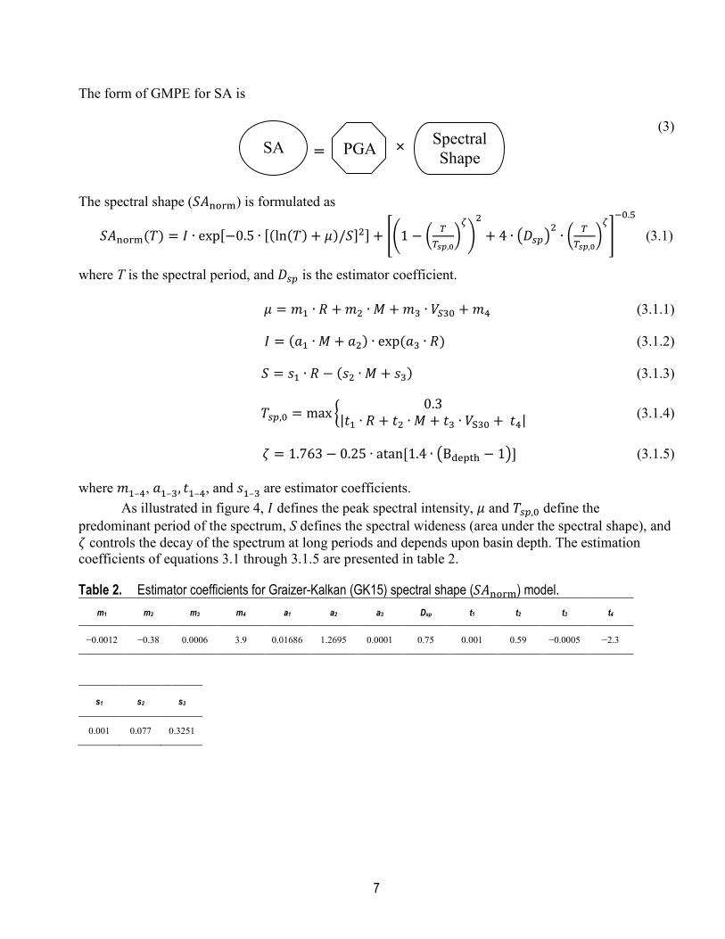
(3)

The spectral shape (𝑆𝐴norm) is formulated as

𝑆𝐴norm(𝑇) = 𝐼 ∙ exp[−0.5 ∙ [(ln(𝑇) + 𝜇)/𝑆]2] + ��1 − � 𝑇𝑇𝑠𝑠,0

�𝜁�2

+ 4 ∙ �𝐷𝑠𝑠�2∙ � 𝑇

𝑇𝑠𝑠,0�𝜁�−0.5

(3.1)

where T is the spectral period, and 𝐷𝑠𝑠 is the estimator coefficient.

𝜇 = 𝑚1 ∙ 𝑅 + 𝑚2 ∙ 𝑀 + 𝑚3 ∙ 𝑉𝑆30 + 𝑚4 (3.1.1) 𝐼 = (𝑎1 ∙ 𝑀 + 𝑎2) ∙ exp (𝑎3 ∙ 𝑅) (3.1.2)

𝑆 = 𝑅1 ∙ 𝑅 − (𝑅2 ∙ 𝑀 + 𝑅3) (3.1.3) 𝑇𝑠𝑠,0 = max � 0.3

|𝑡1 ∙ 𝑅 + 𝑡2 ∙ 𝑀 + 𝑡3 ∙ 𝑉S30 + 𝑡4| (3.1.4)

𝜁 = 1.763 − 0.25 ∙ atan [1.4 ∙ �Bdepth − 1�] (3.1.5) where 𝑚1–4, 𝑎1–3, 𝑡1–4, and 𝑅1–3 are estimator coefficients.

As illustrated in figure 4, 𝐼 defines the peak spectral intensity, 𝜇 and 𝑇𝑠𝑠,0 define the predominant period of the spectrum, S defines the spectral wideness (area under the spectral shape), and 𝜁 controls the decay of the spectrum at long periods and depends upon basin depth. The estimation coefficients of equations 3.1 through 3.1.5 are presented in table 2.

Table 2. Estimator coefficients for Graizer-Kalkan (GK15) spectral shape (𝑆𝐴norm) model. m1 m2 m3 m4 a1 a2 a3 Dsp t1 t2 t3 t4

−0.0012 −0.38 0.0006 3.9 0.01686 1.2695 0.0001 0.75 0.001 0.59 −0.0005 −2.3

s1 s2 s3

0.001 0.077 0.3251

8

Figure 4. Graph showing the generic spectral shape (𝑆𝐴norm) model used and its controlling parameters (I, S, µ,Tsp,0). Note that PGA = peak ground acceleration.

Filter Functions

The physical aspects of each filter function in equation 2 are described below.

G1=Magnitude and Style of Faulting

The following scaling function models the ground-motion scaling owing to the magnitude and style of faulting.

𝐺1 = (𝑐1 ∙ arctan(𝑀 + 𝑐2) + 𝑐3) ∙ 𝐹 (4)

where, 𝑐1, 𝑐2, and 𝑐3 are the estimator coefficients, and F is the style of faulting scaling term. This scaling function reflects the saturation of ground-motion amplitudes with increasing magnitudes. According to the results of Sadigh and others (1997), reverse fault events create ground motions approximately 28 percent higher than those from crustal strike-slip faults. Following this, we used F=1.0 for strike-slip and normal faults, F=1.28 for reverse faults, and F=1.14 for combination of strike-slip and reverse faulting. The 𝐺1 and its estimation coefficients are same as in Graizer and Kalkan (2007).

G2=Distance Attenuation

One of the important features of our GMPE is the use of frequency-response function of a damped single-degree-of-freedom oscillator for modeling the distance attenuation of ground motion. This modeling approach is explained in detail in Graizer and Kalkan (2007). Following this approach, the 𝐺2 models the ground-motion distance attenuation as

𝐺2 = 1 ÷ �(1 − 𝑅/𝑅0 )2 + 4 ∙ (𝐷0)2 ∙ (𝑅/𝑅0 ) (5)

9

where 𝑅0 is the corner distance in the near-source of an earthquake defining the plateau where the ground motion does not attenuate noticeably. In other words, 𝑅0 defines the flat region of the attenuation curve. 𝑅0 is directly proportional to earthquake magnitude—the larger the magnitude, the wider the plateau. The ground-motion observations show that 𝑅0 varies from 4 km for magnitude 5.0 to 10 km for magnitude 7.9 (Graizer and Kalkan, 2007). 𝑅0 is similar to the corner frequency of the Brune’s model (1970, 1971) since both are related to the magnitude.

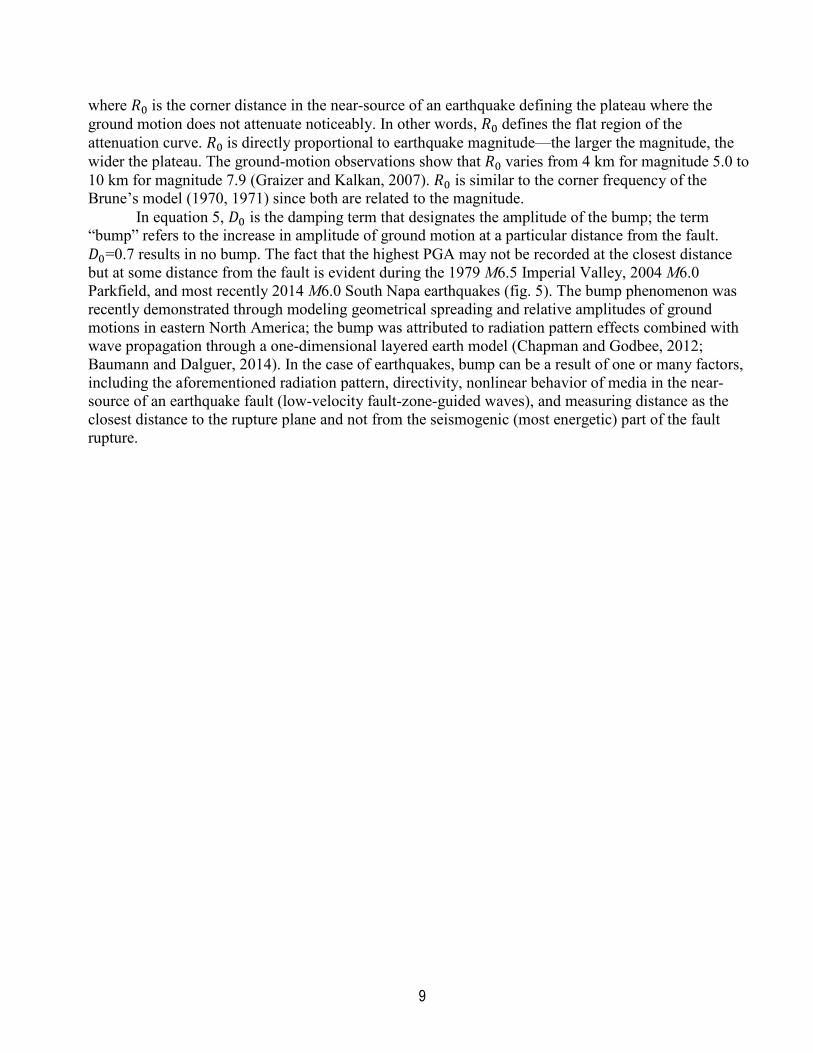
In equation 5, 𝐷0 is the damping term that designates the amplitude of the bump; the term “bump” refers to the increase in amplitude of ground motion at a particular distance from the fault. 𝐷0=0.7 results in no bump. The fact that the highest PGA may not be recorded at the closest distance but at some distance from the fault is evident during the 1979 M6.5 Imperial Valley, 2004 M6.0 Parkfield, and most recently 2014 M6.0 South Napa earthquakes (fig. 5). The bump phenomenon was recently demonstrated through modeling geometrical spreading and relative amplitudes of ground motions in eastern North America; the bump was attributed to radiation pattern effects combined with wave propagation through a one-dimensional layered earth model (Chapman and Godbee, 2012; Baumann and Dalguer, 2014). In the case of earthquakes, bump can be a result of one or many factors, including the aforementioned radiation pattern, directivity, nonlinear behavior of media in the near-source of an earthquake fault (low-velocity fault-zone-guided waves), and measuring distance as the closest distance to the rupture plane and not from the seismogenic (most energetic) part of the fault rupture.

10

Figure 5. Plots showing attenuation of maximum component ground motions during the 2004 magntiude (M) 6.0 Parkfield, 1979 M6.5 Imperial Valley, and 2014 M6.0 South Napa earthquakes. Graphs show amplified peak ground acceleration (PGA) as a bump at near field (R<10 km); this phenomenon is captured well by Graizer-Kalkan (GK15). Note: solid line is for median, dashed lines are for 16th and 84th percentile predictions (R=closest fault distance to rupture plane; VS30=average shear-wave velocity in the upper 30 m of the geological profile).

11

G3=Anelastic Attenuation

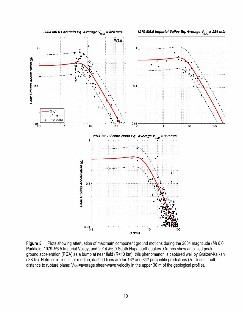
The 𝐺3 function in the Graizer and Kalkan (2007) GMPE for PGA was a simple scaling term to account for attenuation at large distances and basin effects. This term is now replaced with an anelastic attenuation term.

𝐺3 = exp(−𝑐10 ∙ 𝑅/𝑄0) (6)

where 𝑄0 is the regional quality factor for propagation of seismic waves from source to site at 1 Hz, and 𝑐10 is the estimator coefficient. The value for 𝑄0 is, on average, 150 for California and 640–1,000 for central and northeast United States (Singh and Herrmann, 1983; Mitchell and Hwang, 1987; Erickson and others, 2004).

Figure 6A demonstrates the effects of G3 on PGA estimation; the PGA data are from the 1999 M7.6 Chi-Chi earthquake. The earlier version of the G3 in Graizer and Kalkan (2007), denoted as GK07, results in a constant attenuation rate (R-1.5) at large distances (shown by grey line). The black, red, and blue lines are for GK15 with G3 in equation 6 using 𝑄0=75, 150, and 300, respectively. It is clear that a lower crustal 𝑄0 results in faster attenuation, and a higher 𝑄0 yields slower attenuation at far distances.

Q associated with strong motion is different from seismological measurements because the typical seismological Lg and Coda wave estimates of Q sample different volumes of the crust surrounding the station and different paths than typical propagation paths of strong-motion signals (Trifunac, 1994). Trifunac demonstrated that the strong-motion Q increases from very low values near the fault (Q=20 associated with the upper part of the soil profile with relatively low shear-wave velocity) to larger values at about 100–200 km away from the source associated with typical crustal attenuation. For the 2004 M6.0 Parkfield earthquake, frequency independent Q increased from 20 in the upper 300 m of the soil profile to higher values of 100–200 for depth range of 200 m to 5 km (Abercrombie, 2000).

Although Q is distance dependent, 𝑄0 in equation 6 is a constant. In Figure 6B, we made a simple assumption that Q increases with distance from a relatively low value of 10 in the vicinity of the fault to higher values of typical Lg-type crustal Q at far distances (R>100 km). Figure 6C compares the effects of constant 𝑄0 with that of the distance-dependent Q. As expected, low 𝑄0 in the near-source region produces slightly lower ground-motion intensity. However, this decrease does not exceed 3 percent at distances up to 50 km. Higher 𝑄0 at far distances results in slower attenuation relative to the constant 𝑄0. The effect of distance-dependent Q relative to the constant (distance-independent) 𝑄0 is not significant. Considering other uncertainties, we concluded that it is reasonable to use a constant 𝑄0 typical for a given region (usually that for Lg or Coda waves).

In our updated GMPE for PGA, we assume a frequency-independent 𝑄0. In equation 6, 𝑐10=0.345, based on average value of 𝑄0=150 published for California to produce similar effects as our previous GMPE for distances of up to 200 km (shown in fig. 6A). We expect that our GMPE for PGA can be adjusted to other active tectonic regions similar to California by using 𝑄0 values typical for that region and determined using Lg or Coda waves.

12

Figure 6. Graphs showing model results for anelastic attenuation with constant and variable Q0. A, Comparison of Graizer and Kalkan (GK07-09) peak ground acceleration (PGA) predictions with Graizer-Kalkan (GK15) considering the 1999 magnitude (M) 7.6 Chi-Chi earthquake data. B, Constant and distance-dependent Q0. C, Comparison of attenuation curves with constant and distance-dependent Q0 for an M7.0 event (VS30=400 m/s) (R=closest fault distance to rupture plane).

13

G4=Site Correction

Based on published studies (a list of references is given in Graizer and Kalkan, 2007), a linear site-correction filter was adopted in GK07 because of the large variability in nonlinear site-correction models.

𝐺4 = exp [𝑏𝑣 ∙ In(𝑉S30/𝑉𝐴)] (7)

Equation 7 is an equivalent form of the linear site-correction formula of Boore and others (1997), where bv=−0.371, whereas our estimates yield bv=−0.24. Equation 7, with its parameters given in table 1, is similar to the equation of Field (2000) in exhibiting less amplification as VS30 decreases than that of Boore and others (1997). In our revised GMPE for PGA, there is no change in 𝐺4 from its earlier version in Graizer and Kalkan (2007).

G5=Basin Effect

A basin consists of alluvial deposits and sedimentary rocks that are geologically younger and have a significantly lower shear-wave velocity structure than the underlying rocks, which creates a strong interface. A number of publications show that the basin amplifies earthquake-induced body and surface waves (for example, Hanks, 1975; Lee and others, 1995; Campbell, 1997; Frankel and others, 2001). Our new basin scaling function considers combined effects of amplification of both shear and surface waves owing to basin depth under the site according to Hruby and Beresnev (2003) and Day and others (2008). For simplicity, the basin shape and distance to the basin edge (Joyner, 2000; Semblat and others, 2002; Choi and others, 2005) are not accounted for.

The mechanisms and results of shear and surface-wave amplifications in the basin are different. The basin amplification of S-waves affects mostly frequencies lower than ~10 Hz (Hruby and Beresnev, 2003), and basin amplification of surface waves affects a range of spectral frequencies (from PGA to long spectral periods). During the 1992 M7.3 Landers, 1999 M7.1 Hector Mine, and 2010 M7.2 El Mayor-Cucapah earthquakes, the PGA values observed in Los Angeles and San Bernardino basins were much higher than those measured at rock sites owing to amplified surface waves (Graizer and others, 2002; Hatayama and Kalkan, 2012).

In our previous GMPE, the spectral shape decayed at long periods with a slope of T-1.5 (T=spectral period), averaging basin and nonbasin effects (Graizer and Kalkan, 2009). We changed this by implementing the following basin scaling filter, which is a function of depth to 1.5-km/s shear-wave velocity isosurface Z1.5 (Bdepth), R, and T.

𝐺5 = 1 + 𝐴Bdist ∙ 𝐴Bdepth (8)

𝐴Bdepth = 1.077 /��1 − (1.5/(𝐵depth + 0.1))2�2

+ 4 ∙ 0.72 ∙ �1.5/(𝐵depth + 0.1)�2 (8.1)

𝐴Bdist = 1 /�[1 − (40/(𝑅 + 0.1))2]2 + 4 ∙ 0.72 ∙ (40/(𝑅 + 0.1))2 (8.2) Equations 8.1 and 8.2 (previously given as 2.5.1 and 2.5.2) are repeated here for convenience.

𝐴Bdepth defines the amplitude of the basin effect depending upon 𝐵depth. The parameters of equations

14

Equations 8.1 and 8.2 were constrained according to the 1999 M7.1 Hector Mine, M7.3 Landers, and 1989 M6.9 Loma Prieta earthquakes.

As shown in figure 7A, 𝐴𝐵depth varies from 0 for nonbasin to 1.077 for deep basin, and it saturates for basins deeper than 3 km. When 𝐵𝑑𝑑𝑠𝑑ℎ is zero, 𝐴𝐵depthbecomes negligibly small, and the G5 does not have any effect (G5=1.0). It should be noted that our approach on modeling the basin effect is based on the three-dimensional simulations of Day and others (2008). They found that depth to the 1.5-km/s S-wave velocity isosurface is a suitable parameter for use in GMPEs. Similar basin amplification was observed in the Northridge and Whittier Narrows earthquakes by Hruby and Beresnev (2003). Our dependence of period amplification on Z1.5 approximates the period dependence in table 3 of Hruby and Beresnev (2003).

Figure 7. Graphs showing A, dependence of amplitude on basin depth, and B, dependence of the response spectrum long period decay term (𝜁) on basin depth (Bdepth).

The parameter controlling decay rate of spectrum at long periods (ζ in equation 3.1.5) varies in the range of 1.4 to 2. As shown in figure 7B, the spectral shape decays at long periods faster (T-2) for nonbasin sites and slower (T-1.4) for deep basin sites. Figure 8 compares the spectral accelerations for two different basin depths, Bdepth=1.5 and 3 km against the case without basin (Bdepth=0). The deeper

15

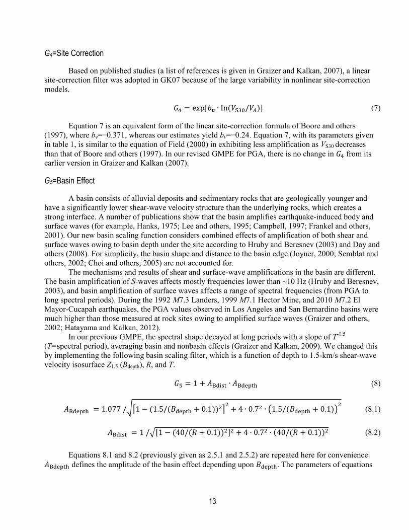
basin produces a response spectrum with higher amplitudes at all periods with slower decay at long periods; it affects the long periods more than the short periods. Based on a three-dimensional modeling of ground motion, a possible explanation for the distance-dependent pattern was suggested by Olsen (2000). According to Olsen, the amplification factors are greater for events located farther from the basin edge. He suggested that the larger-amplitude surface waves generated for the distant events, in part at basin edges, are more prone to the amplification than are the predominant body waves impinging onto the basin sediments from nearby earthquakes.

Figure 8. Graphs showing comparison of pseudo spectral acceleration (SA) response computed using updated Graizer-Kalkan ground-motion prediction equation (GK15) for three cases: nonbasin, basin with 1.5-km depth, and basin with 3-km depth. Background data is from the 1999 magnitude (M) 7.1 Hector Mine earthquake at about 80-km closest fault distance to the fault rupture plane (R). Note that Bdepth =depth to basin.

Mixed-Effects Residuals Analysis We performed a mixed-effects residuals analysis to confirm that GK15 is not biased with respect

to M, R, VS30, and Bdepth by examining trends of residuals against these independent parameters. The residuals at each spectral period are computed as follows:

𝑅𝑅𝑅𝑖𝑖 = ln𝑌𝑖𝑖 − 𝜇𝑖j(𝑀,𝑅,𝑉S30,𝐵depth) (9)

16

where i is the event and j is the recording index. 𝑅𝑅𝑅𝑖𝑖 is the residual of the jth recording of the ith event. 𝑌𝑖𝑖 is the intensity measure (PGA or 5-percent damped pseudo spectral acceleration ordinates) from jth recording of the ith event. Term 𝜇𝑖j represents the GK15’s median (that is, geometric mean4) estimate in natural logarithmic units. In order to check for overall bias, we used the maximum-likelihood method to recursively determine the mean of data points having the error structure of Joyner and Boore (1993), where the residuals correspond to an equation of

𝑅𝑅𝑅𝑖𝑖 = 𝐶 + 𝜂𝑖 + 𝜀𝑖𝑖 (10)

where C is a constant term (maximum-likelihood mean) from the mixed-effects analysis, which is a measure of the overall bias between the observations and the GMPE. The constant term (C) should be close to zero for unbiased estimates. In equation 10, 𝜂𝑖 represents the event term for event i, and 𝜀𝑖𝑖 represents the intra-event residual for recording j in event i. Event term 𝜂𝑖 represents the approximate mean offset of the data for event i from the predictions provided by the median of the GMPE. Event terms (𝜂𝑖) are used to evaluate the GMPE’s performance relative to source predictor variables. Both event and intra-event (within-event) terms are random Gaussian variables with zero mean. Their standard deviations are indicated by 𝜏 and 𝜙, respectively.

For each spectral period, equation 10 is solved using the maximum-likelihood formalism given in the appendix of Spudich and others (1999). In Figure 9, maximum-likelihood mean values are plotted for each spectral period ranging from PGA to 5.0 s; figure 9 shows that the overall bias of GK15 is small. Some discrepancies are plausible because a continuous function of spectral period was forced to fit to all spectral acceleration data instead of a discrete data fitting at each spectral period as other GMPE developers have done.

Figure 9. Plot showing overall mean bias of Graizer-Kalkan (GK15) and its standard deviation; maximum-likelihood mean C shows the overall bias between the observations and predictions.

4For a log-normal distribution of a random variable, the geometric mean (�̂�) and median (𝑥50) are given by the same equation: 𝑥50 = �̂� = 𝑅𝜇, where 𝜇 is the mean of a log-normal distribution Therefore, it is not misleading to use median instead of geometric mean.

17

Close examination of figure 9 indicates that mean bias at PGA and spectral accelerations at 0.2 and 1.0 s is near zero. Increased variability at long periods is consistent with other GMPEs (for example, Abrahamson and others, 2013; Boore and others, 2013) because spectral acceleration data at long periods demonstrate larger aleatory variations than at short periods. At long periods, longer than 2.5 s, GK15 overestimates the data on average by about 0.1 in natural logarithmic units, or about 10 percent. The underestimation between 0.2 and 1.0 s is similar, and it is on average by about 10 percent. The overall bias is negligible for PGA.

In order to separate inter-event disparities from intra-event variations, we performed a mixed-effects analysis with respect to M, R, VS30, and Bdepth, and we fit a slope a and intercept b to residuals according to the following formulation:

𝑅𝑅𝑅𝑖𝑖 = 𝑎 + 𝑏𝑥𝑖 + 𝜂𝑖 + 𝜀𝑖𝑖 (11)

Both slope and intercept computed using equation 11 are plotted against the spectral period in order to check for systematic bias with respect to the independent parameters. Figure 10 shows distance bias in the residuals; again both intercept and slope are near zero for all periods, indicating negligible distance dependence of GK15. Figure 11 shows that there is no systematic magnitude bias in the residuals of GK15; both intercept and slope are essentially zero across the entire period band. In figures 12 and 13, the dependence of GK15 on VS30 and Bdepth are examined; these plots show that slope of fit is essentially zero for VS30 and Bdepth. Although varying degrees of VS30 and Bdepth dependence at certain periods (for example, 0.4 and 3 s) are noticeable, this small dependence is not surprising because VS30 and Bdepth are the two parameters with the least accuracy in the dataset. Overall, small a values indicate that GK15 does not show overprediction or underprediction for the broad range of periods; thus, it is essentially unbiased.

18

Figure 10. Plots showing distance dependence of Graizer-Kalkan (GK15) residuals. Intercept (a) and slope (b) of maximum-likelihood line fit through residuals as a function of closest fault distance to rupture plane (R). Note that y-axis scale is different in top and bottom panels.

19

Figure 11. Plots showing magnitude dependence of Graizer-Kalkan (GK15) residuals. Intercept (a) and slope (b) of maximum-likelihood line fit through residuals as a function of magnitude (M). Note that y-axis scale is different in top and bottom panels.

20

Figure 12. Plots showing VS30 dependence of Graizer-Kalkan (GK15) residuals. Intercept (a) and slope (b) of maximum-likelihood line fit through residuals as a function of VS30. Note that y-axis scale is different in top and bottom panels (VS30=average shear-wave velocity in the upper 30 m of the geological profile).

21

Figure 13. Plots showing depth to basin (Bdepth) dependence of Graizer-Kalkan (GK15) residuals. Intercept (a) and slope (b) of maximum-likelihood line fit through residuals as a function of Bdepth. Note that y-axis scale is different in top and bottom panels.

Intra-Event (Within-Event) Residuals Analysis of Path, Site, and Basin Depth Effects

The intra-event residuals (𝜀𝑖𝑖) are used to test the GK15 with respect to distance and site effects. The residuals are shown in natural logarithmic units for PGA and spectral periods at 0.2, 1.0, and 3.0 s, similar to Chio and Youngs (2013). In figure 14, we plot the intra-event residuals against R (0 to 150 km) using the full dataset, with means and standard errors shown within bins. The bin sizes were adjusted so that each bin has approximately the same number of data points. The maximum-likelihood line is dashed, and its slope and intercept are provided on top of each plot. Although data are slightly underpredicted at 1.0 and 3.0 s for distances greater than 110 km, the results generally show no perceptible trend within the body of a predictor, indicating that the path-scaling functions in GK15 reasonably represent the data trends.

The linear site response analyses consider trends of residuals ij with VS30. The intra-event residuals are plotted against VS30 (200 to 1,200 m/s) in figure 15. At 1.0 s, we note a slight overestimation for VS30 in the range 470 to 560 m/s; we believe that this is in part caused by the sparseness of data within this VS30 range. This overestimation trend is negligible for PGA and spectral

22

acceleration at 0.2 s. In each figure, the flatness of the trends (dashed line) for VS30 indicates that our linear site response function (applicable for VS30>200 m/s) is a reasonable average for shallow crustal continental regions.

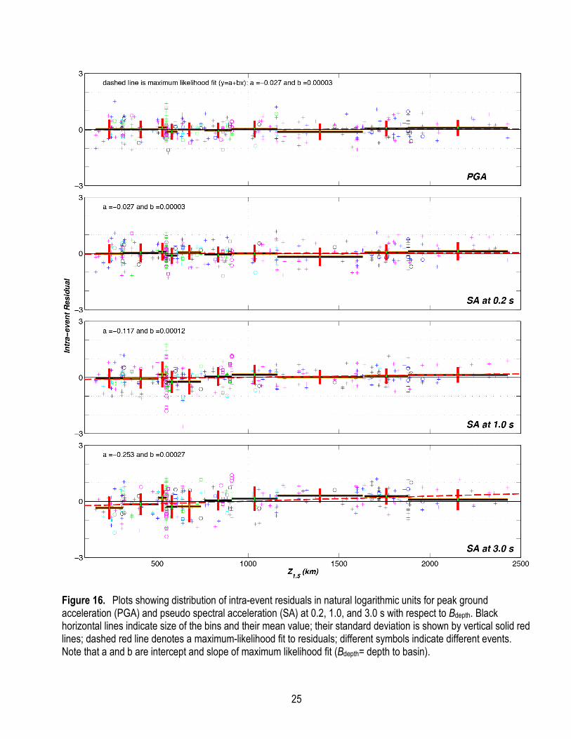
To examine possible sediment depth effects, we plot intra-event residuals in figure 16 against Bdepth in the range 0 to 2,500 m. In general, these residuals do not exhibit notable trends since they are near zero; there is little dependence on Bdepth between 1,200 and 1,400 m at 0.2 and 3.0 s; this is again attributed to the scarcity of the data within this range. It should be noted that number of data points contributing to these plots are less than those provided in previous figures because approximately 15 percent of data in our dataset have known Bdepth.

23

Figure 14. Plots showing distribution of intra-event residuals in natural logarithmic units for peak ground acceleration (PGA) and pseudo spectral acceleration (SA) at 0.2, 1.0, and 3.0 s with respect to closest fault distance to rupture plane (R). Black horizontal lines indicate size of the bins and their mean value; their standard deviation is shown by vertical solid red lines; dashed red line denotes a maximum-likelihood fit to residuals; different symbols indicate different events. Note that a and b are intercept and slope of maximum likelihood fit.

24

Figure 15. Plots showing distribution of intra-event residuals in natural logarithmic units for peak ground acceleration (PGA) and pseudo spectral acceleration (SA) at 0.2, 1.0, and 3.0 s with respect to VS30. Black horizontal lines indicate size of the bins and their mean value; their standard deviation is shown by vertical solid red lines; dashed red line denotes a maximum-likelihood fit to residuals; different symbols indicate different events. Note that a and b are intercept and slope of maximum likelihood fit. (VS30=average shear-wave velocity in the upper 30 m of the geological profile).

25

Figure 16. Plots showing distribution of intra-event residuals in natural logarithmic units for peak ground acceleration (PGA) and pseudo spectral acceleration (SA) at 0.2, 1.0, and 3.0 s with respect to Bdepth. Black horizontal lines indicate size of the bins and their mean value; their standard deviation is shown by vertical solid red lines; dashed red line denotes a maximum-likelihood fit to residuals; different symbols indicate different events. Note that a and b are intercept and slope of maximum likelihood fit (Bdepth= depth to basin).

26

Analysis of Source Effects Using Inter-event (Between-Event) Residuals

In figure 17, we show event terms (𝜂𝑖) plotted against magnitude for PGA and SA at 0.2, 1.0, and 3.0 s using 35 events in the range 4.9≤M≤7.9; the list of these events is given in table 3. The majority of the events, especially at small magnitudes, are from California. The events with less than five data points were excluded; this reduced the number of events from 47 to 35. In figure 17, the maximum-likelihood line is dashed, and its slope and intercept are provided on top of each plot. We see that our magnitude-scaling function (G1) captures the trends from various events as evident by near-zero intercept and near-zero slope of the maximum-likelihood fit, indicating that there is no significant trend with magnitude or a notable offset from zero. Except for the 2003 M6.5 San Simeon and 2004 Parkfield earthquakes, shown by and ∗, respectively, all other 33 events exhibit an event term less than 1.0 (𝜂𝑖<1.0). <The event terms are provided in table 3 for PGA and SA at 0.2, 1.0, and 3.0 s.

27

Figure 17. Plots showing distribution of event terms (𝜂𝑖) in natural logarithmic units for peak ground acceleration (PGA) and pseudo spectral acceleration (SA) at 0.2, 1.0, and 3.0 s with respect to moment magnitude (M); in each plot dashed red line indicates a maximum-likelihood fit to event terms, its slope and intercept are provided on top of each plot. Note that a and b are intercept and slope of maximum likelihood fit.

28

Table 3. Event terms (𝜂𝑖) using 35 events in the magnitude range of 4.9 to 7.9. [See appendix A for details of earthquakes. No, number of event listed in alphabetical order; s, second; PGA, peak ground acceleration]

No Event Event Term (𝜼𝒊)

PGA 0.2 s 1.0 s 3.0 s

1 Anza 0.45 0.58 0.02 −0.76

2 Big Bear City −0.22 0.06 0.70 0.73

3 Borrego Mnt. 0.22 0.18 0.44 0.80

4 Chalfant Valley −0.33 −0.20 −0.25 0.15

5 Chi-Chi (Taiwan) −0.31 −0.37 0.08 0.29

6 Coalinga-01 −0.07 −0.34 0.40 0.33

7 Coalinga-05 0.29 0.18 0.00 0.10

8 Coyote Lake 0.04 −0.02 0.33 0.21

9 Denali (Alaska) −0.23 −0.11 −0.51 −0.34

10 Düzce (Turkey) −0.84 −0.72 −0.87 −0.71

11 Friuli (Italy) −0.12 −0.13 −0.31 −0.34

12 Gulf of California −0.12 −0.32 0.21 0.60

13 Hector Mine 0.12 −0.09 −0.39 −0.83

14 Imperial Valley −0.31 −0.22 −0.26 0.30

15 Kocaeli (Turkey) −0.05 0.04 0.06 0.31

16 Landers −0.23 −0.16 0.02 0.20

17 Lazio-Abruzzo (Italy) −0.10 0.04 −0.01 −0.50

18 Little Skul Mtn. (Nevada) −0.28 −0.20 −0.77 −0.63

19 Livermore −0.06 −0.02 0.44 0.78

20 Loma Prieta −0.02 0.05 0.26 0.30

21 Mammoth Lakes-06 0.39 0.28 0.08 −0.09

22 Manjil (Iran) 0.52 0.56 0.47 0.94

23 Morgan Hill −0.39 −0.45 −0.24 −0.33

24 Northridge −0.06 0.09 −0.03 −0.33

25 North Palm Springs 0.00 0.06 −0.37 −0.57

26 Parkfield −0.21 −0.10 −0.35 0.09

27 Parkfield (2004) −0.23 −0.99 −1.99 −2.33

28 San Fernando −0.42 −0.26 −0.55 −0.31

29 San Simeon 1.71 1.43 2.17 2.47

30 Sierra Madre 0.61 0.58 0.33 0.09

31 Superstition Hills-02 0.03 −0.08 0.11 0.47

32 Taiwan, Smart(5) 0.15 0.27 0.29 0.29

33 Whittier Narrows 0.04 0.23 −0.05 −0.55

34 Yountville −0.35 −0.35 0.60 0.27

35 Yucaipa 0.37 0.53 −0.05 −1.13

29

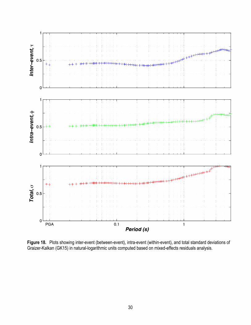
Terms of Standard Deviation In GMPEs, total residuals are composed of intra-event residuals and event terms. The standard

deviation (𝜎) of total residuals (that is, total aleatory variability) is defined as

𝜎 = �𝜏2 + 𝜙2 (12)

Figure 18 plots the inter-event standard deviations (𝜏), intra-event standard deviations (𝜙), and total standard deviations (𝜎) in natural logarithmic units (their values are tabulated in table 4). Figure 18 shows that at long periods, there is likely energy content in the ground motions affecting the single-degree-of-freedom oscillator response, thus increasing the response variability and associated standard deviations. 𝜎 increases with period similar to the NGA-West2 GMPEs (for example, Abrahamson and others, 2014; Boore and others, 2014; Chiou and Youngs, 2014). For short periods (from 0.01 s to 0.3 s), 𝜎 is almost constant.

Recall that our GMPE for spectral shape is a continuous function of spectral period. To be consistent with this continuous form, we model the total aleatory variability (𝜎) with a continuous function of spectral period (T) as

𝜎(𝑇) = max �0.668 + 0.0047 ∙ log(𝑇)

0.8 + 0.13 ∙ log(𝑇) � (13)

Figure 19 compares the approximated 𝜎 using equation 13 with the actual 𝜎. The approximation function matches well with the actual 𝜎 at all periods.

The first stage of the variance analysis is to examine the magnitude dependence of inter-event standard deviations (𝜏) and intra-event standard deviations (𝜙). Figures 20 and 21 show the values of 𝜏 and 𝜙 in natural logarithmic units computed from the residuals, considering eight magnitude bins. These figures show binned values of 𝜏 and 𝜙 for PGA and spectral acceleration ordinates at 0.2, 1.0, and 3.0 s, considering residuals for all magnitudes in the range 4.9≤M≤7.9. In these figures, each bin has an equal number of data points; the ranges of bins are plotted with dashed black lines. The results shown in figure 20 indicate lower values of 𝜏 for larger magnitudes at all periods. The fitted values of 𝜏 demonstrate some level of magnitude dependence at most periods; therefore, a trilinear form is applied. The appropriate magnitude breakpoint is at 7.1 because most of the change occurs between magnitudes of approximately 7.0 and 7.5. The following magnitude-dependent model represents the inter-event standard deviations (𝜏):

𝜏(𝑀) = � 𝑅1 for 𝑀 ≤ 7.1 𝑅1 + (𝑅2−𝑅1) ∙ (𝑀 − 7.1) for 7.1 < 𝑀 < 7.5 𝑅2 for 𝑀 ≥ 7.5

(14)

Terms 𝑅1 and 𝑅2 change slightly with spectral period; their values are provided in table 5.

30

Figure 18. Plots showing inter-event (between-event), intra-event (within-event), and total standard deviations of Graizer-Kalkan (GK15) in natural-logarithmic units computed based on mixed-effects residuals analysis.

31

Table 4. Inter-event standard deviations (𝜏), intra-event standard deviations (𝜙), and total standard deviations (𝜎) in natural logarithmic units.

Period (s) τ ϕ σ Period (s) τ ϕ σ

PGA 0.435 0.508 0.669 0.350 0.415 0.567 0.702

0.010 0.416 0.510 0.658 0.360 0.417 0.568 0.704

0.020 0.422 0.510 0.662 0.380 0.421 0.569 0.708

0.022 0.428 0.512 0.667 0.400 0.425 0.570 0.711

0.025 0.432 0.514 0.671 0.420 0.428 0.569 0.712

0.029 0.436 0.516 0.675 0.440 0.432 0.569 0.714

0.030 0.440 0.518 0.680 0.450 0.432 0.570 0.715

0.032 0.442 0.520 0.682 0.460 0.433 0.571 0.716

0.035 0.444 0.522 0.685 0.480 0.435 0.571 0.718

0.036 0.445 0.524 0.687 0.500 0.437 0.572 0.720

0.040 0.446 0.525 0.689 0.550 0.443 0.572 0.724

0.042 0.447 0.526 0.691 0.600 0.450 0.573 0.729

0.044 0.448 0.527 0.692 0.650 0.457 0.576 0.735

0.045 0.448 0.528 0.692 0.667 0.460 0.580 0.740

0.046 0.449 0.528 0.693 0.700 0.468 0.585 0.749

0.048 0.448 0.528 0.693 0.750 0.480 0.589 0.760

0.050 0.450 0.528 0.693 0.800 0.490 0.591 0.768

0.055 0.451 0.528 0.694 0.850 0.502 0.592 0.776

0.060 0.452 0.527 0.694 0.900 0.515 0.593 0.786

0.065 0.452 0.527 0.695 0.950 0.530 0.596 0.797

0.067 0.453 0.528 0.695 1.000 0.543 0.597 0.807

0.070 0.453 0.528 0.696 1.100 0.562 0.598 0.820

0.075 0.451 0.528 0.695 1.200 0.579 0.598 0.833

0.080 0.449 0.528 0.693 1.300 0.595 0.598 0.844

0.085 0.446 0.528 0.691 1.400 0.609 0.597 0.853

0.090 0.443 0.528 0.689 1.500 0.620 0.599 0.862

0.095 0.440 0.527 0.687 1.600 0.626 0.603 0.869

0.100 0.438 0.528 0.686 1.700 0.632 0.606 0.876

0.110 0.435 0.528 0.685 1.800 0.633 0.610 0.879

0.120 0.431 0.529 0.683 1.900 0.635 0.616 0.885

0.130 0.429 0.530 0.682 2.000 0.635 0.624 0.890

0.133 0.426 0.531 0.680 2.200 0.639 0.634 0.900

0.140 0.423 0.532 0.680 2.400 0.640 0.648 0.911

0.150 0.422 0.534 0.681 2.500 0.644 0.671 0.930

0.160 0.420 0.536 0.681 2.600 0.650 0.693 0.950

0.170 0.419 0.536 0.680 2.800 0.656 0.710 0.967

0.180 0.414 0.536 0.678 3.000 0.660 0.718 0.975

0.190 0.410 0.539 0.677 3.200 0.665 0.719 0.979

0.200 0.407 0.541 0.677 3.400 0.673 0.719 0.984

32

Period (s) τ ϕ σ Period (s) τ ϕ σ

0.220 0.407 0.544 0.679 3.500 0.680 0.723 0.992

0.240 0.409 0.547 0.683 3.600 0.683 0.722 0.994

0.250 0.408 0.550 0.685 3.800 0.687 0.727 1.000

0.260 0.406 0.554 0.687 4.000 0.682 0.721 0.992

0.280 0.407 0.558 0.690 4.200 0.680 0.715 0.986

0.290 0.405 0.561 0.692 4.400 0.676 0.717 0.985

0.300 0.406 0.564 0.694 4.600 0.670 0.718 0.982

0.320 0.410 0.565 0.698 4.800 0.667 0.718 0.980

0.340 0.414 0.566 0.701 5.000 0.699 0.745 1.022

Figure 19. Plot showing total standard deviations (σ) of Graizer-Kalkan (GK15) and its approximation in natural logarithmic units.

The 𝜙 values shown in figure 21 demonstrate that the intra-event standard deviations are stable with small variations over a wide range of magnitudes. In these figures, colored lines denote the population mean, which is close to the mean values of the bins. A complex relationship of intra-event standard deviations with magnitude at 3 s is apparent. However, for PGA and spectral acceleration ordinates at periods of 0.2 and 1 s, intra-event standard deviations seem to be magnitude independent.

33

Figure 20. Plots showing values of inter-event (between-event) standard deviations (𝜏) computed for peak ground acceleration (PGA) and pseudo spectral acceleration (SA) at 0.2, 1.0, and 3.0 s in magnitude bins with equal number of data points; magnitude (M) range for each bin is shown by a horizontal black dashed line; colored lines denote the simplified 𝜏 model as a function of M.

34

The distance dependence of 𝜏 and 𝜙 is examined next in figures 22 and 23, respectively. The standard deviation data is divided into ten distance bins and plotted against R. Each bin has an equal number of data points. The inter-event standard deviations (𝜏) rise for the distances larger than 100 km. This is attributed to the regional anelastic attenuation effects that are not fully captured by our model. Thus, we expect that this increase is strongly influenced by epistemic uncertainty in regional attenuation rates, not random site-to-site variability. To identify this variation, we adjust the model in equation 14 to include an additive term that is applicable for R>100 km as follows:

𝜏(𝑀, 𝑅) = �𝜏(𝑀)𝜏(𝑀) + 𝑟1 for 𝑅 ≤ 100 +(𝑟1 − 𝑟2) ∙ (R − 100) for 100 < 𝑅 < 130𝜏(𝑀) + 𝑟2 for 𝑅 ≥ 130

(15)

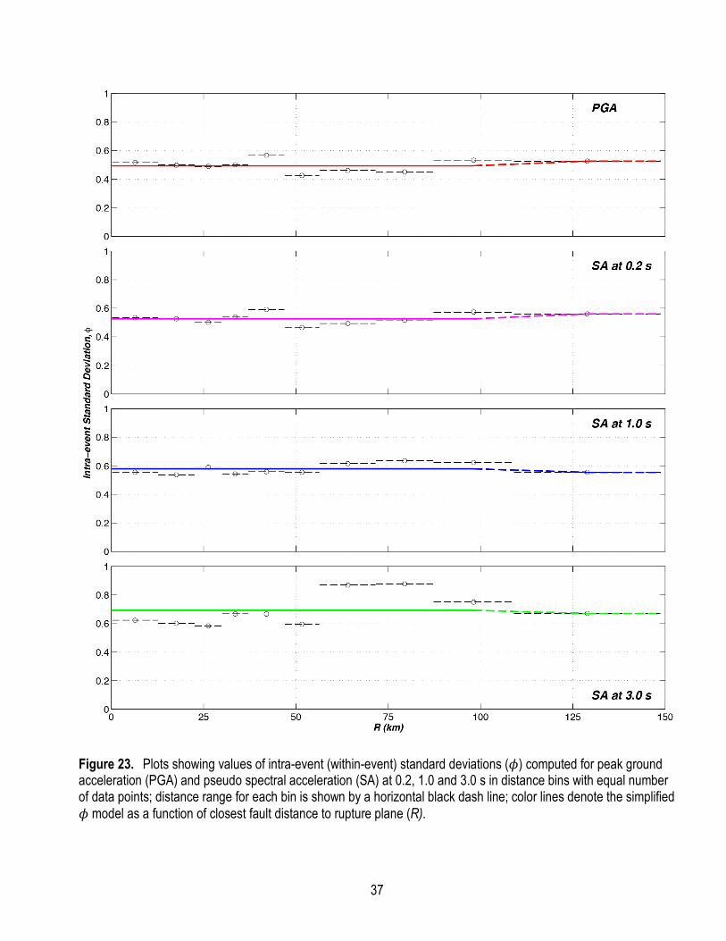
Terms 𝑟1 and 𝑟2 are selected by visual inspection; they represent the maximum distance to which the complete GMPE terms are considered applicable (𝑟1, generally up to 100 km) and the distance beyond which we capped increases with distance (𝑟2 , generally up to 150 km). Figure 23 indicates that 𝜙 is overall independent of R; there are slight variations at large distances.

In figures 24 and 25, we plot the values of 𝜏 and 𝜙 within VS30 bins. Each bin has an equal number of data points. We observe no change in 𝜏 for PGA and short periods. There is a slight variation of 𝜏 with VS30 at long periods above 500 m/s. For 𝜙, there is no significant variation with VS30. This is attributed to the smaller dataset that we used as compared to GMPEs of Abrahamson and others (2013) and Boore and others (2013), which have a VS30 dependence on 𝜏 because the NGA-West2 dataset has only 22 percent of VS30 measured, and the remaining 78 percent of NGA-West2 dataset are from estimations based on correlation of VS30 with local surface geology. Approximately half of the stations in our database have measured VS30, whereas the rest have inferred VS30 values. Overall, 𝜏 is magnitude and distance dependent. For a site with given M and R, 𝜏 can be computed using equation 15 with the parameters 𝑅1, 𝑅2, 𝑟1, and 𝑟2 provided in table 5.

Table 5. Coefficients of inter-event (between-event) standard deviation term. [SA = spectral acceleration]

Peak ground acceleration SA (0.2) SA (1.0) SA (3.0)

s1 0.28 0.26 0.33 0.51

s2 0.04 0.07 0.06 0.06

r1 0.30 0.35 0.31 0.57

r2 0.52 0.50 0.58 0.90

35

Figure 21. Plots showing values of intra-event (within-event) standard deviations (𝜙) computed for peak ground acceleration (PGA) and pseudo spectral acceleration (SA) at 0.2, 1.0 and 3.0 s in magnitude bins with equal number of data points; magnitude (M) range for each bin is depicted by a horizontal black dash line; color lines denote the simplified 𝜙 model as a function of M.

36

Figure 22. Plots showing values of inter-event (between-event) standard deviations (𝜏) computed for peak ground acceleration (PGA) and pseudo spectral accelerations (SA) at 0.2, 1.0 and 3.0 s in distance bins with equal number of data points; distance range for each bin is shown by a horizontal black dash line; color lines denote the simplified 𝜏 model as a function of closest fault distance to rupture plane (R).

37

Figure 23. Plots showing values of intra-event (within-event) standard deviations (𝜙) computed for peak ground acceleration (PGA) and pseudo spectral acceleration (SA) at 0.2, 1.0 and 3.0 s in distance bins with equal number of data points; distance range for each bin is shown by a horizontal black dash line; color lines denote the simplified 𝜙 model as a function of closest fault distance to rupture plane (R).

38

Figure 24. Plots showing values of inter-event (between-event) standard deviations (𝜏) computed for peak ground acceleration (PGA) and pseudo spectral acceleration (SA) at 0.2, 1.0 and 3.0 s in VS30 bins with equal number of data points; VS30 range for each bin is shown by a horizontal black dash line; color lines denote the simplified 𝜏 model as a function of average shear-wave velocity in the upper 30 m of the geological profile (VS30).

39

Figure 25. Plots showing values of intra-event (within-event) standard deviations (𝜙) computed for peak ground acceleration (PGA) and pseudo spectral acceleration (SA) at 0.2, 1.0 and 3.0 s in VS30 bins with equal number of data points; VS30 range for each bin is shown by a horizontal black dash line; color lines denote the simplified 𝜙 model as a function of average shear-wave velocity in the upper 30 m of the geological profile (VS30).

40

Model Results The median SA response spectra for the GK15 model are shown in figure 26 for a vertical strike-

slip earthquake scenario with M=5.0, 6.0, 7.0, and 8.0, at distances R=1 and 30 km, and VS30=760 and 270 m/s, similar to comparisons given in Abrahamson and others (2013). Note that increase in magnitude shifts the predominant period of spectrum to larger values. The predominant period in our spectral shape model is controlled by μ and Tsp,0 as shown in figure 4, and both of them are magnitude dependent. A wider spectrum generated by larger magnitudes implies that energy at different periods is enriched by the complex wave propagation.

The path scaling is shown next in figure 27 for PGA and spectral periods at 0.3, 1.0, and 3.0 s. In this figure, the median ground motion from strike-slip earthquakes on rock site condition (VS30=760 m/s) is shown for four different magnitudes, M=5.0, 6.0, 7.0, and 8.0. At intermediate distance range (5 to 20 km from the fault), the GK15 model produces higher acceleration values. These high accelerations look like a bump on the attenuation curves. The reason for this bump was explained in section “G2=Distance Attenuation.”

The magnitude scaling of the current model is shown in figure 28 for vertical strike-slip earthquakes on rock site conditions (VS30=760 m/s) for T=0.2, 1.0, and 3.0 s at distances R=1, 30, and 150 km. Note that the break in the magnitude scaling at M5.5 is driven by consistency in response spectra of recorded data. The weak scaling of the short-period motion at short distances reflects the saturation with magnitude.

The site response scaling for an M7.0 vertical strike-slip earthquake at a closest rupture distance of 30 km is demonstrated in figure 29. The decrease in shear-wave velocity amplifies ground motion and shifts the predominant period to higher spectral periods. Based on the same rupture scenario, figure 30 displays the dependence of the spectra on Bdepth for a soil site with VS30=270 m/s.

The style of faulting scaling on the SA response spectra is shown in figure 31 for an M7.0 vertical strike-slip earthquake at a rupture distance of 30 km for a soil site with VS30=270 m/s. Lastly, Q0 is shown in figure 32 for PGA and spectral periods at 0.3, 1.0, and 3.0 s. The median ground motion from an M7.0 strike-slip earthquake on rock site condition (VS30=760 m/s) is shown for four different Q0. Figure 33 demonstrates the effects of Q0 on SA response spectra. The higher Q0 results in higher acceleration values. As Q0 increases, its effect on SA diminishes for all periods.

41

Figure 26. Graphs showing comparison of median pseudo spectral accelerations (SA) for strike-slip magnitude (M) 5.0, 6.0, 7.0, and 8.0 earthquakes at R=1 and 30 km and VS30=270 and 760 m/s considering Q0=150 and Bdepth=0 (R=closest fault distance to rupture plane; VS30=average shear-wave velocity in the upper 30 m of the geological profile; Q0=quality factor; Bdepth= depth to basin).

42

Figure 27. Graphs showing comparison of distance scaling for strike-slip magnitude (M) 5.0, 6.0, 7.0, and 8.0 earthquakes at median PGA and pseudo spectral accelerations at 0.2, 1.0, and 3.0 s considering VS30=760 m/s, Q0=150 and Bdepth=0 (R=closest fault distance to rupture plane; VS30=average shear-wave velocity in the upper 30 m of the geological profile; Q0=quality factor; Bdepth= depth to basin).

43

Figure 28. Graphs showing comparison of magnitude scaling for strike-slip earthquakes at closest fault distance to rupture plane, R=1, 30, and 150 km for median peak ground acceleration (PGA) and pseudo spectral accelerations (SA) at 0.3, 1.0, and 3.0 s considering VS30=760 m/s, Q0=150 and Bdepth=0 (R=closest fault distance to rupture plane; VS30=average shear-wave velocity in the upper 30 m of the geological profile; Q0=quality factor; Bdepth= depth to basin).

44

Figure 29. Graph showing comparison of VS30 scaling on pseudo spectral accelerations (SA) for a strike-slip magntitude (M) 7.0 earthquake at R=30 km considering Q0=150 and Bdepth=0 (VS30=average shear-wave velocity in the upper 30 m of the geological profile; Q0=quality factor; Bdepth= depth to basin).

Figure 30. Graph showing comparison of Bdepth scaling on pseudo spectral accelerations (SA) for a strike-slip M7.0 earthquake at R=30 km considering Q0=150 and VS30=270 m/s (R=closest fault distance to rupture plane; VS30=average shear-wave velocity in the upper 30 m of the geological profile; Q0=quality factor; Bdepth= depth to basin).

45

Figure 31. Graph showing comparison of style of faulting scaling on pseudo spectral accelerations (SA) for a magnitude (M) 7.0 earthquake at R=30 km considering Q0=150, VS30=270 m/s, and Bdepth=0 (R=closest fault distance to rupture plane; VS30=average shear-wave velocity in the upper 30 m of the geological profile; Q0=quality factor; Bdepth= depth to basin).

46

Figure 32. Graphs showing comparison of Q0 scaling with closest fault distance to rupture plane (R) for a strike-slip magnitude (M) 7.0 earthquake for median peak ground acceleration (PGA) and pseudo spectral accelerations (SA) at 0.3, 1.0, and 3.0 s considering VS30=760 m/s and Bdepth=0 (VS30=average shear-wave velocity in the upper 30 m of the geological profile; Q0=quality factor; Bdepth= depth to basin).

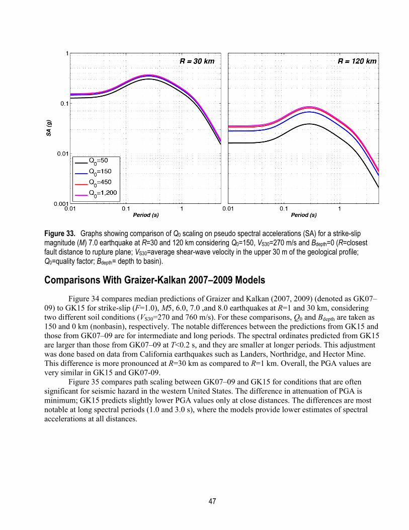
47

Figure 33. Graphs showing comparison of Q0 scaling on pseudo spectral accelerations (SA) for a strike-slip magnitude (M) 7.0 earthquake at R=30 and 120 km considering Q0=150, VS30=270 m/s and Bdepth=0 (R=closest fault distance to rupture plane; VS30=average shear-wave velocity in the upper 30 m of the geological profile; Q0=quality factor; Bdepth= depth to basin).

Comparisons With Graizer-Kalkan 2007–2009 Models Figure 34 compares median predictions of Graizer and Kalkan (2007, 2009) (denoted as GK07–

09) to GK15 for strike-slip (F=1.0), M5, 6.0, 7.0 ,and 8.0 earthquakes at R=1 and 30 km, considering two different soil conditions (VS30=270 and 760 m/s). For these comparisons, Q0 and Bdepth are taken as 150 and 0 km (nonbasin), respectively. The notable differences between the predictions from GK15 and those from GK07–09 are for intermediate and long periods. The spectral ordinates predicted from GK15 are larger than those from GK07–09 at T<0.2 s, and they are smaller at longer periods. This adjustment was done based on data from California earthquakes such as Landers, Northridge, and Hector Mine. This difference is more pronounced at R=30 km as compared to R=1 km. Overall, the PGA values are very similar in GK15 and GK07-09.

Figure 35 compares path scaling between GK07–09 and GK15 for conditions that are often significant for seismic hazard in the western United States. The difference in attenuation of PGA is minimum; GK15 predicts slightly lower PGA values only at close distances. The differences are most notable at long spectral periods (1.0 and 3.0 s), where the models provide lower estimates of spectral accelerations at all distances.

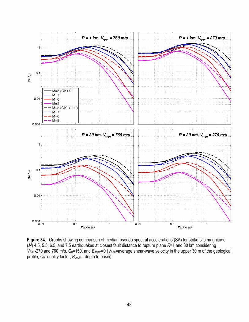
48

Figure 34. Graphs showing comparison of median pseudo spectral accelerations (SA) for strike-slip magnitude (M) 4.5, 5.5, 6.5, and 7.5 earthquakes at closest fault distance to rupture plane R=1 and 30 km considering VS30=270 and 760 m/s, Q0=150, and Bdepth=0 (VS30=average shear-wave velocity in the upper 30 m of the geological profile; Q0=quality factor; Bdepth= depth to basin).

49

Figure 35. Graphs showing comparison of distance scaling for strike-slip magnitude (M) 5.0, 6.0, 7.0, and 8.0 earthquakes at median peak ground acceleration (PGA) and pseudo spectral accelerations (SA) at 0.2, 1.0, and 3.0 s considering VS30=760 m/s, Q0=150, and Bdepth=0 (R=closest fault distance to rupture plane; VS30=average shear-wave velocity in the upper 30 m of the geological profile; Q0=quality factor; Bdepth= depth to basin).

Figure 36 compares total aleatory variability in the present study to those of GK07–09. The total aleatory variability from the present study is generally higher at all periods than of GK07–09. We attribute the higher σ to the way that we computed total aleatory variability in GK15, by the method provided in Joyner and Boore (1993), which uses two random variables (εr and εe) replaced by a single

50

random variable ε as in GK07–09. The higher σ could result from the triangle inequality and the lack of correlation between random variables εr and εe (P. Spudich, U.S. Geological Survey, oral commun., 2014).

Figure 36. Plot showing comparison of total aleatory variability (σ) between Graizer-Kalkan (2007, 2009) (GK07–09) and Graizer-Kalkan (GK15) ground-motion prediction equations.

Comparisons With NGA-West2 Models We compare the model predictions of GK15 with those of Abrahamson and others (2014)

(abbreviated as ASK14) and Boore and others (2014) (abbreviated as BSSA14). Figures 37 and 38 compare the median attenuation of PGA and spectral accelerations at 0.2, 1.0, and 3.0 s for horizontal motions for a vertically dipping strike-slip earthquake as a function of closest distance to fault rupture. These results are for VS30=760 m/s. Visual comparison of the predictions of our model with those of the two NGA-West2 relationships shows that our predictions are in good agreement with the predictions of ASK14 and BSSA14 for a range of magnitudes and distances. For PGA and SA at 0.2 s, GK15 produces similar or slightly lower results as compared to the BSSA14 and ASK14 at close distances (0–5 km). At intermediate distances (5–20 km), the GK15 produces higher values because of the bump.

The response spectra from magnitude 6.0, 7.0, and 8.0 earthquakes at R=1 and 30 km from a vertically dipping strike-slip fault and VS30=270 and 760 m/s are plotted in figures 39 and 40. The same parameters used in figures 37 and 38 were repeated. There is similarity among the three models for the M6–8 cases. The difference between models increases for the M8 case, especially at the long spectral periods.

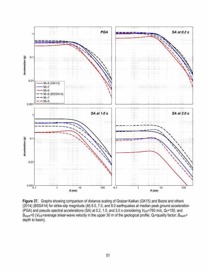
51

Figure 37. Graphs showing comparison of distance scaling of Graizer-Kalkan (GK15) and Boore and others (2014) (BSSA14) for strike-slip magnitude (M) 6.0, 7.0, and 8.0 earthquakes at median peak ground acceleration (PGA) and pseudo spectral accelerations (SA) at 0.2, 1.0, and 3.0 s considering VS30=760 m/s, Q0=150, and Bdepth=0 (VS30=average shear-wave velocity in the upper 30 m of the geological profile; Q0=quality factor; Bdepth= depth to basin).

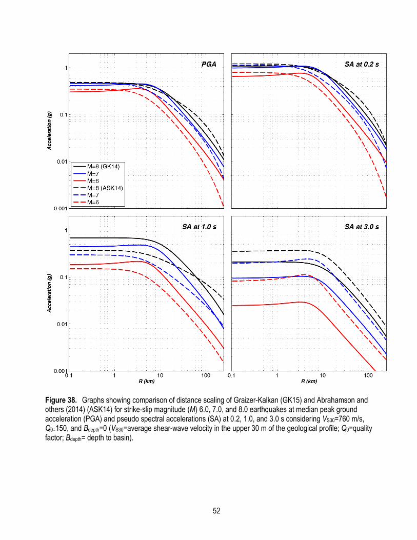
52

Figure 38. Graphs showing comparison of distance scaling of Graizer-Kalkan (GK15) and Abrahamson and others (2014) (ASK14) for strike-slip magnitude (M) 6.0, 7.0, and 8.0 earthquakes at median peak ground acceleration (PGA) and pseudo spectral accelerations (SA) at 0.2, 1.0, and 3.0 s considering VS30=760 m/s, Q0=150, and Bdepth=0 (VS30=average shear-wave velocity in the upper 30 m of the geological profile; Q0=quality factor; Bdepth= depth to basin).

53

Figure 39. Graphs showing comparison of spectra from Graizer-Kalkan (GK15) and Boore and others (2014) (BSSA14) for strike-slip magnitude (M) 6.0, 7.0, and 8.0 earthquakes at closest fault distance to rupture plane R =1 and 30 km, considering VS30=270 and 760 m/s, Q0=150, and Bdepth=0 (VS30=average shear-wave velocity in the upper 30 m of the geological profile; Q0=quality factor; Bdepth= depth to basin).

54

Figure 40. Graphs showing comparison of spectra from Graizer-Kalkan (GK15) and Abrahamson and others (2014) (ASK14) for strike-slip magnitude (M) 6.0, 7.0, and 8.0 earthquakes at closest fault distance to rupture plane R =1 and 30 km, considering VS30=270 and 760 m/s, Q0=150, and Bdepth=0 (VS30=average shear-wave velocity in the upper 30 m of the geological profile; Q0=quality factor; Bdepth= depth to basin).

55

Comparisons With Earthquake Data In figures 41–53, distance attenuation curves by GK15 for PGA and spectral accelerations at 0.2,

1.0, and 3.0 s are plotted against the ground-motion data from 13 major events in California, Alaska, Taiwan, and Turkey. The results are based on randomly oriented maximum horizontal component of ground motions; average VS30 of dataset was used for each event. Figures are presented in chronological order of earthquakes. Visual comparison of predictions derived from the GK15 with observations reveal a reasonable to excellent performance of the revised model for a range of magnitudes and distances.

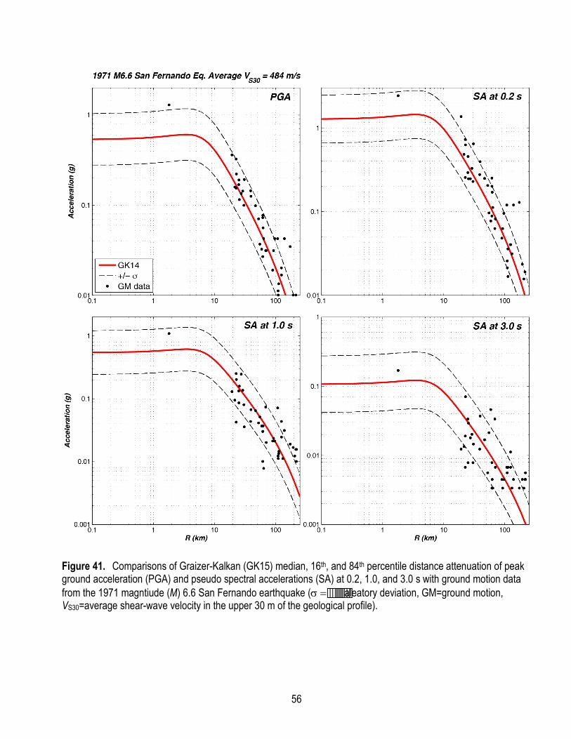
56

Figure 41. Comparisons of Graizer-Kalkan (GK15) median, 16th, and 84th percentile distance attenuation of peak ground acceleration (PGA) and pseudo spectral accelerations (SA) at 0.2, 1.0, and 3.0 s with ground motion data from the 1971 magntiude (M) 6.6 San Fernando earthquake (σ =aleatory deviation, GM=ground motion, VS30=average shear-wave velocity in the upper 30 m of the geological profile).

57

Figure 42. Comparisons of Graizer-Kalkan (GK15) median, 16th, and 84th percentile distance attenuation of peak ground acceleration (PGA) and pseudo spectral accelerations (SA) at 0.2, 1.0, and 3.0 s with ground motion data from the 1979 magntiude (M) 6.5 Imperial Valley earthquake (σ = total aleatory variability, GM=ground motion, VS30=average shear-wave velocity in the upper 30 m of the geological profile).

58

Figure 43. Comparisons of Graizer-Kalkan (GK15) median, 16th, and 84th percentile distance attenuation of peak ground acceleration (PGA) and pseudo spectral accelerations (SA) at 0.2, 1.0, and 3.0 s with ground motion data from the 1989 magntiude (M) 6.9 Loma Prieta earthquake (σ = total aleatory variability, GM=ground motion, VS30=average shear-wave velocity in the upper 30 m of the geological profile).

59

Figure 44. Comparisons of Graizer-Kalkan (GK15) median, 16th, and 84th percentile distance attenuation of peak ground acceleration (PGA) and pseudo spectral accelerations (SA) at 0.2, 1.0, and 3.0 s with ground motion data from the 1992 magntiude (M) 7.3 Landers earthquake (σ = total aleatory variability, GM=ground motion, VS30=average shear-wave velocity in the upper 30 m of the geological profile).

60

Figure 45. Comparisons of Graizer-Kalkan (GK15) median, 16th, and 84th percentile distance attenuation of peak ground acceleration (PGA) and pseudo spectral accelerations (SA) at 0.2, 1.0, and 3.0 s with ground motion data from the 1994 magntiude (M) 6.4 Northridge earthquake (σ = total aleatory variability, GM=ground motion, VS30=average shear-wave velocity in the upper 30 m of the geological profile).

61

Figure 46. Comparisons of Graizer-Kalkan (GK15) median, 16th, and 84th percentile distance attenuation of peak ground acceleration (PGA) and pseudo spectral accelerations (SA) at 0.2, 1.0, and 3.0 s with ground motion data from the 1999 magntiude (M) 7.1 Hector Mine earthquake (σ = total aleatory variability, GM=ground motion, VS30=average shear-wave velocity in the upper 30 m of the geological profile)

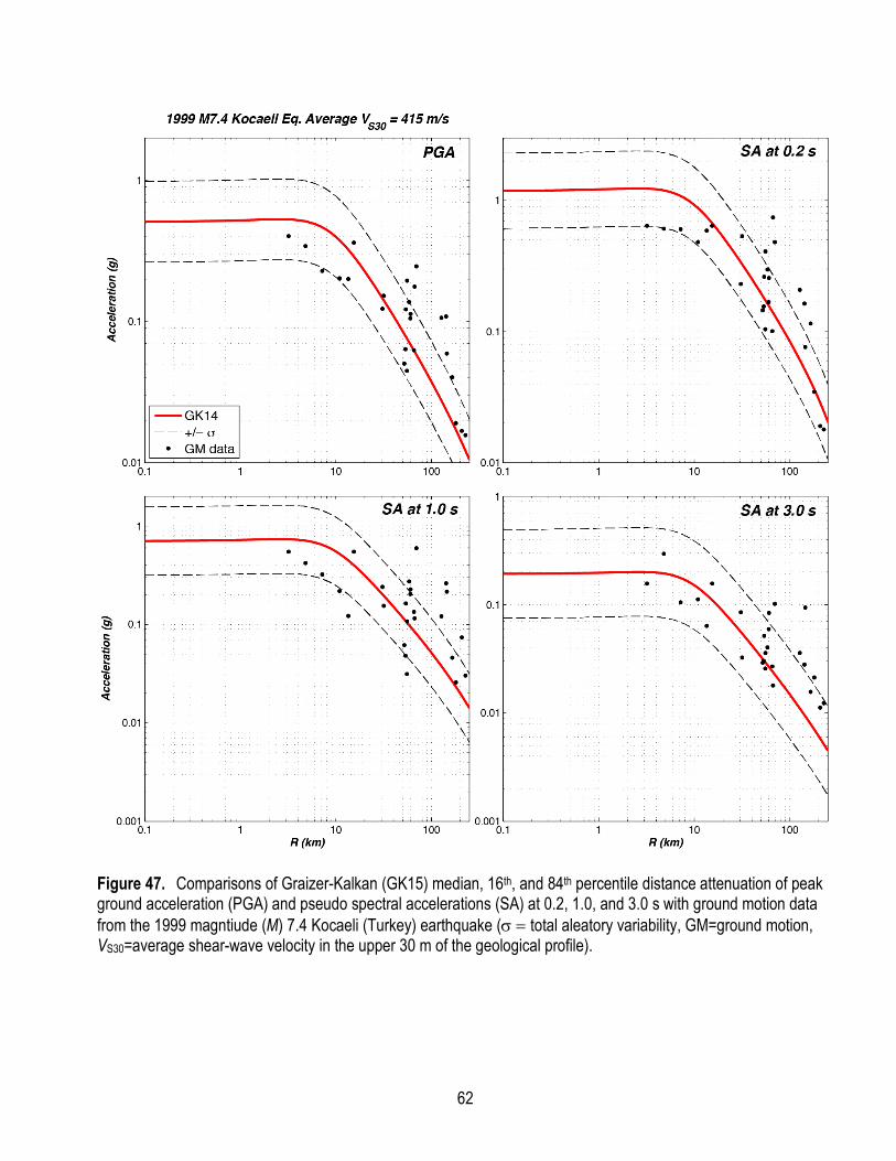
62

Figure 47. Comparisons of Graizer-Kalkan (GK15) median, 16th, and 84th percentile distance attenuation of peak ground acceleration (PGA) and pseudo spectral accelerations (SA) at 0.2, 1.0, and 3.0 s with ground motion data from the 1999 magntiude (M) 7.4 Kocaeli (Turkey) earthquake (σ = total aleatory variability, GM=ground motion, VS30=average shear-wave velocity in the upper 30 m of the geological profile).

63

Figure 48. Comparisons of Graizer-Kalkan (GK15) median, 16th, and 84th percentile distance attenuation of peak ground acceleration (PGA) and pseudo spectral accelerations (SA) at 0.2, 1.0, and 3.0 s with ground motion data from the 1999 magnitude (M) 7.2 Düzce (Turkey) earthquake (σ = total aleatory variability, GM=ground motion, VS30=average shear-wave velocity in the upper 30 m of the geological profile).

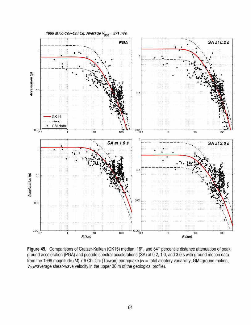
64

Figure 49. Comparisons of Graizer-Kalkan (GK15) median, 16th, and 84th percentile distance attenuation of peak ground acceleration (PGA) and pseudo spectral accelerations (SA) at 0.2, 1.0, and 3.0 s with ground motion data from the 1999 magnitude (M) 7.6 Chi-Chi (Taiwan) earthquake (σ = total aleatory variability, GM=ground motion, VS30=average shear-wave velocity in the upper 30 m of the geological profile).

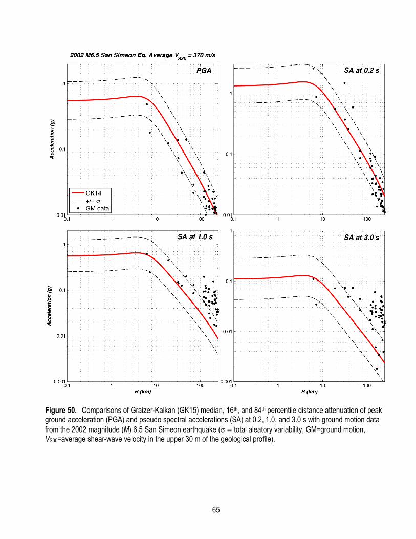
65

Figure 50. Comparisons of Graizer-Kalkan (GK15) median, 16th, and 84th percentile distance attenuation of peak ground acceleration (PGA) and pseudo spectral accelerations (SA) at 0.2, 1.0, and 3.0 s with ground motion data from the 2002 magnitude (M) 6.5 San Simeon earthquake (σ = total aleatory variability, GM=ground motion, VS30=average shear-wave velocity in the upper 30 m of the geological profile).

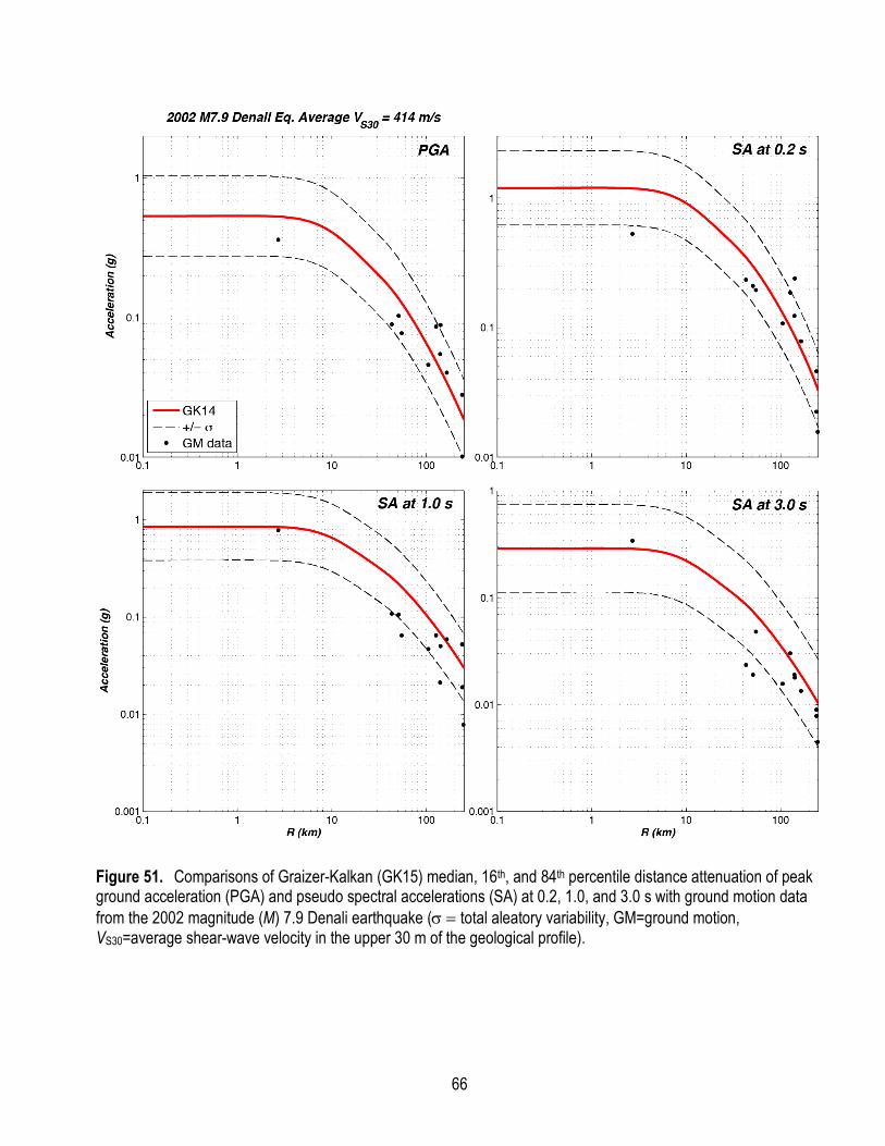
66

Figure 51. Comparisons of Graizer-Kalkan (GK15) median, 16th, and 84th percentile distance attenuation of peak ground acceleration (PGA) and pseudo spectral accelerations (SA) at 0.2, 1.0, and 3.0 s with ground motion data from the 2002 magnitude (M) 7.9 Denali earthquake (σ = total aleatory variability, GM=ground motion, VS30=average shear-wave velocity in the upper 30 m of the geological profile).

67

Figure 52. Comparisons of Graizer-Kalkan (GK15) median, 16th, and 84th percentile distance attenuation of peak ground acceleration (PGA) and pseudo spectral accelerations (SA) at 0.2, 1.0, and 3.0 s with ground motion data from the 2004 magnitude (M) 6.0 Parkfield earthquake (σ = total aleatory variability, GM=ground motion, VS30=average shear-wave velocity in the upper 30 m of the geological profile).

68

Figure 53. Comparisons of Graizer-Kalkan (GK15) median, 16th, and 84th percentile distance attenuation of peak ground acceleration (PGA) and pseudo spectral accelerations (SA) at 0.2, 1.0, and 3.0 s with ground motion data from the 2014 magnitude (M) 6.0 South Napa earthquake (σ = total aleatory variability, GM=ground motion, VS30=average shear-wave velocity in the upper 30 m of the geological profile).

69

Example Calculations Using MatLAB Codes The GK15 GMPE is coded as a MatLAB function (titled “GK15.m”) in appendix B. An example

MatLAB code (“runGK15.m”) to generate a 5-percent damped pseudo spectral acceleration response spectrum for a given hazard condition is provided in appendix C. Running this code generates the spectrum shown in figure 54 for a vertically dipping strike-slip M6.0 event at a site with VS30=350 m/s and 4.4 km away from the rupture plane. The user can change the input parameters to construct a site-specific response spectrum considering different hazard conditions.

Figure 54. Site-specific 5-percent damped pseudo spectral acceleration (SA) response spectra generated using the MatLAB code in appendix C for a vertically dipping strike-slip magnitude (M) 6.0 earthquake at closest fault distance to rupture plane (R)=4.4 km considering VS30=350 m/s, Q0=150, and Bdepth=0 (σ = total aleatory variability, VS30=average shear-wave velocity in the upper 30 m of the geological profile; Q0=quality factor; Bdepth= depth to basin).

Range of Applicability The GMPE update developed in this study is considered to be applicable for estimating pseudo

spectral accelerations (5 percent of critical damping) in the period range of 0.01 to 5 s and peak motions for earthquakes in which the following conditions apply:

70

• magnitude (M), 5.0–8.0; • distance (R), 0–250 km; • time-averaged shear-wave velocity (VS30), 200–1,300 m/s; • Q0, up to 250, typical for active tectonic environment; and • basin depth (Bdepth), 0–10 km.

These limits are based on the distributions of the data used to develop the GK15 GMPE. The GMPE presented in this report is intended for application in western United States or in similar tectonically active shallow crustal regions. The data controlling the equations are derived principally from California; we have also used ground-motion data from Nevada, Alaska, Turkey, Taiwan, Italy, Armenia, Georgia, and Uzbekistan. Implementation of the GK15 to other active crustal regions may result in an additional degree of epistemic uncertainty.

The site and basin effects incorporated into the GK15 GMPE provide an average representation on specified values of VS30 and Bdepth. Some sites may show significant differences from these average site and basin effects. These differences are particularly likely when the geologic structure of the site is appreciably different than the average of the dataset.

For application in other active tectonic regions where earthquakes at distances greater than about 50 km are a major contributor to seismic hazard, there is a need for the user to obtain estimates of Q0 for that region for accurate ground-motion predictions.

Concluding Remarks In this study, the Graizer-Kalkan ground-motion prediction equation (GMPE) for peak ground

acceleration and 5-percent damped pseudo spectral acceleration response ordinates is revised to account for differences in ground-motion scaling in terms of regional far-source distance attenuation and basin effects. The new GMPE is controlled by a small number of measurable parameters including moment magnitude, closest distance to the fault rupture, style of faulting, shear-wave velocity in the upper 30 m of site geological formation, regional quality factor, and basin depth (defined as the depth to 1.5-km/s shear-wave velocity isosurface).

The Graizer-Kalkan (GK15) offers a much simpler functional form than the NGA-West2 models (for example, Abrahamson and others, 2014 (ASK14); Boore and others, 2014 (BSSA14); Campbell and Bozorgnia, 2014; Chio and Youngs, 2014), and it has either less or comparable standard deviations depending upon the spectral period of interest. The GK15 models spectral acceleration as a continuous function of spectral period, whereas the NGA-West2 models use a discrete functional form to compute SA ordinates at certain periods only (a total of 21 periods from 0.01 to 10 s). Comparisons of the GK15 model with ASK14 and BSSA14 demonstrate that GK15 produces similar or slightly lower results at very close distances to the fault (up to about 5 km) and at distances of more than 20 km from the fault for earthquakes with magnitude larger than 6.0. At intermediate distances (5 to 20 km from the fault), the GK15 produces higher estimates of ground motion than ASK14 and BSSA14.

In conclusion, the GK15 GMPE is a significant improvement over GK07–09, and provides a demonstrable, reliable description of ground-motion amplitudes recorded from shallow crustal earthquakes in active tectonic regions over a wide range of magnitudes, distances and site conditions.

Data and Resources Data used in this study came from published sources listed in the text or in references. The

Graizer-Kalkan (GK15) ground-motion prediction equation is available from the authors upon request in

71

Fortran and Excel. The MatLAB functions for GK15 are provided in appendix B. An example MatLAB routine to generate a site-specific response spectrum for given hazard conditions is provided in appendix C.

Disclaimer Any opinions, findings, and conclusions expressed in this report are those of the authors and do

not necessarily reflect the views of the U.S. Nuclear Regulatory Commission.

References Cited Abercrombie, R.E., 2000, Crustal attenuation and site effects at Parkfield, California: Journal of

Geophysical Research: v. 105, no. B3, p. 6277–6286. Abrahamson, N.A., Silva, W.J., and Kamai, R., 2013, Update of the AS08 ground-motion prediction

equations based on the NGA-West2 data set: Pacific Earthquake Engineering Research Center Report 2013/04, 144 p.

Abrahamson, N.A., Silva, W.J., and Kamai, R., 2014, Summary of the ASK14 Ground Motion Relation for Active Crustal Regions. Earthquake Spectra, v. 30, no. 3, p. 1025–1055.

Baumann, C., and Dalguer, L.A., 2014, Evaluating the compatibility of dynamic rupture-based synthetic ground motion with empirical ground-motion prediction equation: Bulletin of the Seismological Society of America, v. 104, no. 2, p. 634–652.

Boore, D.M., Joyner, W.B., and Fumal, T.E., 1997, Equations for estimating horizontal response spectra and peak acceleration from western North American earthquakes; A summary of recent work: Seismological Research Letters, v. 68, no. 1, p. 128–153.

Boore M.D., Stewart, J.P. Seyhan, E. and Atkinson, G.M., 2013, NGA-West2 equations for predicting response spectral accelerations for shallow crustal earthquakes: Pacific Earthquake Engineering Research Center Report 2013/05, 106 p.

Boore M.D., Stewart, J.P. Seyhan, E. and Atkinson, G.M., 2014, NGA-West2 Equations for Predicting PGA, PGV, and 5% Damped PSA for Shallow Crustal Earthquakes. Earthquake Spectra, v. 30, no. 3, p. 1057–1085.

Brune, J., 1970, Tectonic stress and the spectra of seismic shear waves from earthquakes: Journal of Geophysical Research, v. 75, no. 26, p. 4997–5009.

Brune, J., 1971, Correction: Journal of Geophysical Research, v. 76, no. 20, p. 5002. Campbell, K.W.,1997, Empirical near-source attenuation relations for horizontal and vertical

components of peak ground acceleration, peak ground velocity, and pseudo-absolute acceleration response spectra: Seismological Research Letters, v. 68, no. 1, p. 154–179.

Campbell, K.W., and Bozorgnia, Y., 2008, NGA ground motion model for the geometric mean horizontal component of PGA, PGV, PGD and 5% damped linear elastic response spectra for periods ranging from 0.01 to 10 s: Earthquake Spectra, v. 24, no. 1, p. 139–171.

Campbell, K.W., and Bozorgnia, Y., 2014, NGA-West2 Ground Motion Model for the Average Horizontal Components of PGA, PGV, and 5% Damped Linear Acceleration Response Spectra, Earthquake Spectra, v. 30, no. 3, p. 1087–1115.

Chapman, M.C., and Godbee, R.W., 2012, Modeling geometrical spreading and the relative amplitudes of vertical and horizontal high-frequency ground motions in eastern North America: Bulletin of the Seismological Society of America, v. 102, no. 5, p. 1957–1975.

72

Chiou, B., Darragh, R., Gregor, N., and Silva, W., 2008, NGA project strong-motion database: Earthquake Spectra, v. 24, no. 1, p. 23–44.

Chiou, B., and Youngs, R.R., 2013, Update of the Chiou and Youngs NGA ground motion model for average horizontal component of peak ground motion and response spectra: Pacific Earthquake Engineering Research Center Report 2013/07, 78 p.

Chiou, B., and Youngs, R.R., 2014, Update of the Chiou and Youngs NGA Model for the Average Horizontal Component of Peak Ground Motion and Response Spectra. Earthquake Spectra, v. 30, no. 3, p. 1117–1153.

Choi, Y., Stewart, J.P., and Graves, R.W., 2005, Empirical model for basin effects accounts for basin depth and source location: Bulletin of the Seismological Society of America, v. 95, no. 4, p. 1412–1427.

Day, S.M., Graves, R., Bielak, J., Dreger, D., Larsen, S., Olsen, K.B., Pitarka, A., and Ramirez-Guzman, L., 2008, Model for basin effects on long-period response spectra in Southern California: Earthquake Spectra, v. 24, no. 1, p. 257–277.

Erickson, D., McNamara, D.E., and Benz, H.M., 2004, Frequency-dependent Lg Q within the continental United States: Bulletin of the Seismological Society of America, v. 94, no. 5, p. 1630–1643.

Field, E.H., 2000, A modified ground motion attenuation relationship for Southern California that accounts for detailed site classification and a basin-depth effect: Bulletin of the Seismological Society of America, v. 90, no. 6B, p. S209–S221.

Frankel, A., Carver, D., Cranswick, E., Bice, T., Sell, R., and Hanson, S., 2001, Observation of basin ground-motions from a dense seismic array in San Jose, California: Bulletin of the Seismological Society of America, v. 91, no. 1, p. 1–12.

Graizer, V., Shakal, A., Scrivner, C., Hauksson, E., Polet, J., and Jones, L., 2002, TriNet strong-motion data from the M 7.1 Hector Mine, California, earthquake of 16 October 1999: Bulletin of the Seismological Society of America, v. 92, no. 4, p. 1525–1541.

Graizer, V., and Kalkan, E., 2007, Ground-motion attenuation model for peak horizontal acceleration from shallow crustal earthquakes: Earthquake Spectra, v. 23, no. 3, p. 585–613.

Graizer, V., and Kalkan, E., 2009, Prediction of response spectral acceleration ordinates based on PGA attenuation: Earthquake Spectra, v. 25, no. 1, p. 39–69.

Graizer, V., and Kalkan, E., 2011, Modular filter-based approach to ground-motion attenuation modeling: Seismological Research Letters, v. 82, no. 1, p. 21–31.

Graizer, V., Kalkan, E., and Lin, K.W., 2013, Global ground-motion prediction equation for shallow crustal regions: Earthquake Spectra, v. 29, no. 3, p. 777–791.

Hanks, T.C., 1975, Strong ground motion of the San Fernando, California, earthquake; ground displacements: Bulletin of the Seismological Society of America, v. 65, no. 1, p.193–225.

Hatayama, K., and Kalkan, E., 2012, Spatial amplification of long-period (3 to 16 s) ground-motions in and around the Los Angeles Basin during the 2010 M7.2 El Mayor-Cucapah earthquake: Procedings of the 15th World Conference on Earthquake Engineering, Lisbon, Portugal, 2012, 10 p.

Hruby, C.E., and Beresnev, I.A., 2003, Empirical corrections for basin effect in stochastic ground-motion prediction, based on the Los Angeles basin analysis: Bulletin of the Seismological Society of America, v. 93, no. 4, p. 1679–1690.

Joyner, W.B., and Boore, D.M., 1993, Methods for regression analysis of strong-motion data: Bulletin of the Seismological Society of America, v. 83, no. 2, p. 469–487.

Joyner, W.B., 2000, Strong motion from surface waves in deep sedimentary basins: Bulletin of the Seismological Society of America, v. 90, p. S95–S112.

73

Lee, V.W., Trifunac, M.D., Todorovska, M.I., and Novikova, E.I., 1995, Empirical equations describing attenuation of peak of strong ground-motion, in terms of magnitude, distance, path effects and site conditions: Department of Civil Engineering, University of Southern California, Report No. CE 95–02, 268 p.

Mitchell, B.J., and Hwang, H.J., 1987, Effect of low Q sediments and Crustal Q on Lg attenuation in the United States: Bulletin of the Seismological Society of America, v. 77, no. 4, p. 1197–1210.

Olsen, K.B., 2000, Site amplification in the Los Angeles basin from three-dimensional modeling of ground-motion: Bulletin of the Seismological Society of America, v. 90, no. 6B, p. S77–S94.

Sadigh, K., Chang, C.-Y., Egan, J.A., Makdisi, F., and Youngs, R.R., 1997, Attenuation relationships for shallow crustal earthquakes based on California strong motion data: Seismological Research Letters, v. 68, no. 1, p. 180–189.

Semblat, J.F., Dangla, P., Kham, M., and Duval, A.M., 2002, Seismic effect for shallow and deep alluvial basins; in-depth motion and focusing effect: Soil Dynamics and Earthquake Engineering, v. 22, nos. 9–12, p. 849–854.

Singh, S., and Herrmann, R.B., 1983, Regionalization of crustal coda Q in the continental United States: Journal of. Geophysical Research, v. 88, no. B1, p. 527–538.

Trifunac, M.D., 1994, Q and high-frequency strong motion spectra: Soil Dynamics and Earthquake Engineering, v. 13, p. 149–161.

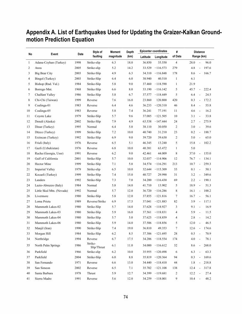
74

Appendix A. List of Earthquakes Used for Updating the Graizer-Kalkan Ground-motion Prediction Equation

No Event Date Style of faulting

Moment magnitude

Depth (km)

Epicenter coordinates # of Data

Distance Range (km) Latitude Longitude

1 Adana-Ceyhan (Turkey) 1998 Strike-slip 6.3 18.0 36.850 35.550 4 28.0 - 96.0

2 Anza 2005 Strike-slip 5.2 14.2 33.529 −116.573 279 4.8 - 197.6

3 Big Bear City 2003 Strike-Slip 4.9 6.3 34.310 −116.848 178 8.6 - 166.7

4 Bingol (Turkey) 2003 Strike-Slip 6.4 6.0 38.940 40.510 1 6.1 5 Bishop (Rnd. Val.) 1984 Strike-Slip 5.8 9.0 37.460 −118.590 1 21.9 6 Borrego Mnt. 1968 Strike-Slip 6.6 8.0 33.190 −116.142 5 45.7 - 222.4

7 Chalfant Valley 1986 Strike-Slip 5.8 6.7 37.577 −118.449 5 6.4 - 24.5

8 Chi-Chi (Taiwan) 1999 Reverse 7.6 16.0 23.860 120.800 420 0.3 - 172.2

9 Coalinga-01 1983 Reverse 6.4 4.6 36.233 −120.310 46 8.4 - 55.8

10 Coalinga-05 1983 Reverse 5.8 7.4 36.241 77.191 11 4.6 - 16.2

11 Coyote Lake 1979 Strike-Slip 5.7 9.6 37.085 −121.505 10 3.1 - 33.8

12 Denali (Alaska) 2002 Strike-Slip 7.9 4.9 63.538 −147.444 24 2.7 - 275.9

13 Dinar (Turkey) 1995 Normal 6.4 5.0 38.110 30.050 2 3.0 - 39.6

14 Düzce (Turkey) 1999 Strike-Slip 7.2 10.0 40.740 31.210 23 0.2 - 188.7

15 Erzincan (Turkey) 1992 Strike-Slip 6.9 9.0 39.720 39.630 2 5.0 - 65.0

16 Friuli (Italy) 1976 Reverse 6.5 5.1 46.345 13.240 5 15.8 - 102.2

17 Gazli (Uzbekistan) 1976 Reverse 6.8 10.0 40.381 63.472 1 5.0 18 Racha (Georgia, Ussr) 1991 Reverse 6.2 9.0 42.461 44.009 8 37.0 - 155.0 19 Gulf of California 2001 Strike-Slip 5.7 10.0 32.037 −114.906 12 76.7 - 134.1

20 Hector Mine 1999 Strike-Slip 7.1 5.0 34.574 −116.291 213 10.7 - 259.3

21 Imperial Valley 1979 Strike-slip 6.5 10.0 32.644 −115.309 33 0.1 - 50.1

22 Kocaeli (Turkey) 1999 Strike-Slip 7.4 15.0 40.727 29.990 31 3.2 - 349.6

23 Landers 1992 Strike-Slip 7.3 7.0 34.200 −116.430 69 2.2 - 190.1

24 Lazio-Abruzzo (Italy) 1984 Normal 5.8 14.0 41.710 13.902 5 18.9 - 51.3

25 Little Skul Mtn. (Nevada) 1992 Normal 5.7 12.0 36.720 −116.286 8 16.1 - 100.2

26 Livermore 1980 Strike-Slip 5.8 12.0 37.855 −121.816 7 16.7 - 56.1

27 Loma Prieta 1989 Reverse/Strike 6.9 17.5 37.041 −121.883 82 3.9 - 117.1

28 Mammoth Lakes-02 1980 Strike-Slip 5.7 14.0 37.628 −118.927 3 9.1 - 16.9

29 Mammoth Lakes-03 1980 Strike-Slip 5.9 16.0 37.561 −118.831 4 5.9 - 11.5

30 Mammoth Lakes-04 1980 Strike-Slip 5.7 5.0 37.625 −118.859 4 2.8 - 14.2

31 Mammoth Lakes-06 1980 Strike-Slip 5.9 14.0 37.506 −118.856 5 12.0 - 46.5

32 Manjil (Iran) 1990 Strike-Slip 7.4 19.0 36.810 49.353 7 12.6 - 174.6

33 Morgan Hill 1984 Strike-Slip 6.2 8.5 37.306 −121.695 28 0.5 - 70.9

34 Northridge 1994 Reverse 6.7 17.5 34.206 −118.554 174 4.0 - 78.1

35 North Palm Springs 1986 Strike-Slip/Thrust 6.1 11.0 34.000 −116.612 32 8.6 - 268.0

36 Parkfield 1966 Strike-slip 6.2 10.0 35.955 −120.498 6 6.3 - 63.3

37 Parkfield 2004 Strike-Slip 6.0 8.8 35.819 −120.364 94 0.3 - 169.6

38 San Fernando 1971 Reverse 6.6 13.0 34.440 −118.410 44 1.8 - 218.8

39 San Simeon 2002 Reverse 6.5 7.1 35.702 −121.108 138 12.4 - 317.8

40 Santa Barbara 1978 Thrust 5.9 12.7 34.399 −119.681 2 12.2 - 27.4

41 Sierra Madre 1991 Reverse 5.6 12.0 34.259 −118.001 9 10.4 - 48.2

75

No Event Date Style of faulting

Moment magnitude

Depth (km)

Epicenter coordinates # of Data

Distance Range (km) Latitude Longitude

42 Spitak (Armenia) 1988 Reverse 6.8 5.0 40.987 44.185 1 25.0 43 Superstition Hills-02 1987 Strike-Slip 6.5 9.0 33.022 −115.831 11 1.0 - 27.0

44 Taiwan, Smart(5) 1981 Reverse 5.9 11.1 24.429 121.896 7 28.7 - 32.0

45 Whittier Narrows 1987 Reverse 6.0 14.6 34.049 −118.081 116 14.5 - 103.9

46 Yountville 2000 Strike-Slip 5.0 10.1 38.379 −122.413 25 9.9 - 95.7

47 Yucaipa 2005 Reverse 4.9 11.6 34.058 −117.011 388 2.6 - 160.1

Total = 2,583

76

Appendix B. MatLAB Code for Graizer-Kalkan Ground-motion Prediction Equation (2015) %% 2015 GRAIZER-KALKAN GMPE % % Graizer & Kalkan 2015 updated GMPE for horizontal component ground motion % % Syntax: % out = GK15(M, R, VS30, F, Q_0, Bdepth,flag) % % Input: % M = Moment magnitude % R = Closest distance to fault rupture in km (i.e., Rrup) % VS30 = Average shear-wave velocity in the upper 30 m in m/s % Bdepth = Depth to 1,500 m/s shear-wave velocity (i.e., Z1.5) % Bdepth = 0 for non-basin sites % F = Style of faulting % F = 1.0 for strike-slip and normal faulting, % F = 1.28 for reverse faulting, and % F = 1.14 for combination of strike-slip and reverse faulting % Q_0 = Regional Q_0 value (e.g., 150 for California) % Bdepth = Depth to 1,500 m/s shear-wave velocity to define basin (i.e., Z1.5) % Bdepth = 0 for non-basin sites % flag = 'm' for maximum horizontal component; 'a' for average % horizontal component % Output: % out = [t,SA,sigma] % t = Spectral period vector (PGA to 5 s) % SA = Median pseudo spectral acceleration ordinates (PGA to SA at 5 s) % Sigma = Total standard deviations % % $Revision: 1.0 $ $Date: 01/18/2015 $ % Written by Dr. Erol Kalkan, P.E. (ekalkan@usgs.gov) % % Comment blocks and equation references in this function correspond to the % following publication: % % Graizer, V. and Kalkan, E. (2015). Update of the Graizer_Kalkan ground-motion % prediction equation for shallow crustal continental earthquakes, % U.S. Geological Survey Open-File Report 2015-1009, p. 98. function [out] = GK15(M,R,VS30,F,Q_0,Bdepth,flag) if flag == 'm'; amp = 1; else amp = 1/1.12; % average to maximum component conversion end %% GMPE for PGA c1 = 0.14; c2 = -6.25; c3 = 0.37; c4 = 2.237; c5 = -7.542; c6 = -0.125; c7 = 1.19; c8 = -6.15; c9 = 0.6; c10 = 0.345; bv = -0.24; VA = 484.5; %% InPGA = G1 + G2 + G3 + G4 + G5;

77

G1 = log(( c1 * atan (M + c2) + c3) * F); Ro = c4*M + c5; Do = c6 * cos(c7 * (M + c8)) + c9; G2 = -0.5 * log((1-R/Ro)^2 + 4 * (Do^2) * (R/Ro)); G3 = -c10 * R / Q_0; G4 = bv * log(VS30 / VA); A_Bdepth = 1.077/sqrt((1-(1.5/(Bdepth+0.1))^2)^2+4*0.7^2*(1.5/(Bdepth+0.1))^2); A_Bdist = 1/sqrt((1-(40/(R+0.1))^2)^2+4*0.7^2*(40/(R+0.1))^2); G5 = log(1 + A_Bdepth * A_Bdist); InPGA = G1 + G2 + G3 + G4 + G5; PGA = exp(InPGA) * amp; %% GMPE for Spectral Shape (GK15SS) t = [0.01 0.02 0.022 0.025 0.029 0.03 0.032 0.035 ... 0.036 0.04 0.042 0.044 0.045 0.046 0.048 0.05 ... 0.055 0.06 0.065 0.067 0.07 0.075 0.08 0.085 ... 0.09 0.095 0.1 0.11 0.12 0.13 0.133 0.14 0.15 ... 0.16 0.17 0.18 0.19 0.2 0.22 0.24 0.25 0.26 ... 0.28 0.29 0.3 0.32 0.34 0.35 0.36 0.38 0.4 ... 0.42 0.44 0.45 0.46 0.48 0.5 0.55 0.6 0.65 ... 0.667 0.7 0.75 0.8 0.85 0.9 0.95 1 1.1 1.2 1.3 1.4 ... 1.5 1.6 1.7 1.8 1.9 2 2.2 2.4 2.5 2.6 2.8 3 3.2 3.4 3.5 3.6 ... 3.8 4 4.2 4.4 4.6 4.8 5]; m1 = -0.0012; m2 = -0.38; m3 = 0.0006; m4 = 3.9; a1 = 0.01686; a2 = 1.2695; a3 = 0.0001; Dsp = 0.75; t1 = 0.001; t2 = 0.59; t3 = -0.0005; t4 = -2.3; s1 = 0.001; s2 = 0.077; s3 = 0.3251; if (M<5.5); M=5.5; end for j = 1:length(t); I = (a1*M+a2)*exp(a3*R); mu = m1*R + m2*M + m3*VS30 + m4; S = s1*R - (s2*M + s3); Tsp_o = max(0.3,abs(t1*R + t2*M + t3*VS30 + t4)); zay = 1.763-0.25*atan(1.4*(Bdepth-1)); F1(j) = I*exp(-0.5*((log(t(j))+mu)/S)^2); F2(j) = 1/sqrt((1-(t(j)/Tsp_o)^zay)^2 + 4*Dsp^2*(t(j)/Tsp_o)^zay); Y(j) = F1(j) + F2(j); end Sigma = max(0.668 + 0.0047 * log(t),0.8 + 0.13 * log(t)); %% SA = GK15SS x exp(GK15PGA) SA = [PGA Y * exp(InPGA) * amp]; t = [0 t]; Sigma = [0.66 Sigma]; %% Output [Spectral Period, SA in "g"] out = [t' SA' Sigma']; return

78

Appendix C. MatLAB Code to Generate Pseudo Spectral Acceleration Response Spectrum Using Graizer-Kalkan 2015 (GK15) Ground-motion Prediction Equation % RUN GRAIZER-KALKAN (GK15) GMPE TO GENERATE 5% DAMPED PSEUDO SPECTRAL % ACCELERATION RESPONSE SPECTRUM % % Syntax: % runGK15 % % Input: % M = Moment magnitude % R = Closest distance to fault rupture in km (i.e., Rrup) % VS30 = Average shear-wave velocity in the upper 30 m in m/s % Bdepth = Depth to 1,500 m/s shear-wave velocity isosurface (i.e., Z1.5) % Bdepth = 0 for non-basin sites % % F = Style of faulting % F = 1.0 for strike-slip and normal faulting, % F = 1.28 for reverse faulting, and % F = 1.14 for combination of strike-slip and reverse faulting % Output: % SA = Median pseudo spectral acceleration (SA) ordinates (PGA to 5 s) % SA_16 = 16th percentile SA % SA_84 = 84th percentile SA % % $Revision: 1.0 $ $Date: 01/18/2015 $ % Written by Dr. Erol Kalkan, P.E. (ekalkan@usgs.gov) % % Comment blocks and equation references in this function correspond to the % following publication: % % Graizer, V. and Kalkan, E. (2015). Update of the Graizer-Kalkan ground-motion % prediction equation for shallow crustal continental earthquakes, % U.S. Geological Survey Open-File Report 2015-1009, p. 98. clear all; clc; close all; flag = input('maximum or average component (enter m or a): ', 's'); % Example Input Parameters M = 6.0; R = 4.4; VS30 = 350; F = 1.0; % Strike-slip fault Bdepth = 0; % No basin Q_0 = 50; % Regional quality factor for Napa, California %% Call GK15 [out] = GK15(M,R,VS30,F,Q_0,Bdepth,flag); t = out(:,1); SA = out(:,2); Sigma = out(:,3); %% SA plus/minus sigma (16th and 84th percentile values) SA_16 = SA./exp(Sigma); SA_84 = SA.*exp(Sigma); PeakSaAmp = max(SA); for j = 1:length(t);

79

if (SA(j) == PeakSaAmp); Tmax = t(j); break end end %% Plot spectrum set(gcf,'position',[300 283 600 350]); set(gca,'TickLength',[.0025 .0025]); loglog(t,SA,'r-','LineWidth',2.5); hold; loglog(t,SA_16,'k--','LineWidth',1.0); legend('SA','+/- \sigma'); loglog(t,SA_84,'k--','LineWidth',1.0); loglog(0.01,SA(1),'o','MarkerSize',12,... 'MarkerEdgeColor','b','MarkerFaceColor','r'); loglog(Tmax,0.001,'o','MarkerSize',12,... 'MarkerEdgeColor','b','MarkerFaceColor','r'); loglog(Tmax,PeakSaAmp,'o','MarkerSize',12,... 'MarkerEdgeColor','b','MarkerFaceColor','r'); axis([0.01 5 0.01 4]); set(gca,'XTickLabel',{'0.01','0.1','1'},'fontsize',12); set(gca,'YTickLabel',{'0.01','0.1','1','4'},'fontsize',12); xlabel('Period (s)','FontSize',[13],'FontWeight','bold','FontAngle','italic'); ylabel('Spectral Acceleration (g)','FontSize',[13],'FontWeight','bold','FontAngle','italic'); tit1 = strcat('{M = }',num2str(M,'%5.1f')); tit2 = strcat('{R = }',num2str(R),' km'); tit3 = strcat('{V_S_3_0 = }',num2str(VS30),' m/s'); text('pos',[0.015 0.045],'str',tit1,'Color','k','FontSize',[12],'FontWeight','bold'); text('pos',[0.015 0.03],'str',tit2,'Color','k','FontSize',[12],'FontWeight','bold'); text('pos',[0.015 0.018],'str',tit3,'Color','k','FontSize',[12],'FontWeight','bold'); text('pos',[0.012 SA(1)*0.8],'str',num2str(SA(1),'%5.2f'),'Color','k','FontSize',[12],'FontWeight','bold'); text('pos',[Tmax PeakSaAmp*1.4],'str',num2str(PeakSaAmp,'%5.2f'),'Color','k','FontSize',[12],'FontWeight','bold'); text('pos',[Tmax*1.2 0.0015],'str',num2str(Tmax),'Color','k','FontSize',[12],'FontWeight','bold'); title('GK15 (5% damped) Pseudo Spectral Acc. Response Spectrum','FontSize',[13],'FontWeight','bold','FontAngle','italic'); hold on; grid on;