unsupervised clustering of neural pathways - inria · unsupervised clustering of neural pathways...
TRANSCRIPT
HAL Id: hal-00908433https://hal.inria.fr/hal-00908433v1
Submitted on 2 Aug 2014 (v1), last revised 4 Jul 2015 (v2)
HAL is a multi-disciplinary open accessarchive for the deposit and dissemination of sci-entific research documents, whether they are pub-lished or not. The documents may come fromteaching and research institutions in France orabroad, or from public or private research centers.
L’archive ouverte pluridisciplinaire HAL, estdestinée au dépôt et à la diffusion de documentsscientifiques de niveau recherche, publiés ou non,émanant des établissements d’enseignement et derecherche français ou étrangers, des laboratoirespublics ou privés.
Unsupervised Clustering of Neural PathwaysSergio Medina
To cite this version:Sergio Medina. Unsupervised Clustering of Neural Pathways. Machine Learning [cs.LG]. 2014. <hal-00908433v1>
Universidad de Buenos AiresFacultad de Ciencias Exactas y Naturales
Departamento de Computación
Unsupervised Clustering of NeuralPathways
Tesis presentada para optar al título deLicenciado en Ciencias de la Computación
Sergio Medina
Director: Bertrand Thirion
Codirector: Gaël Varoquaux
Parietal Team, Inria Saclay, Francia, 2013

AGRUPAMIENTO NO SUPERVISADO DE VÍAS NEURONALES
Las Imágenes de Resonancia Magnética de Difusión (dMRI, por sus siglas en inglés)pueden revelar la micro-estructura de la materia blanca del cerebro.
El análisis de la anisotropía observada en las imágenes dMRI contrastadas con métodosde tractografía pueden ayudarnos a comprender los patrones de conexión entre las distintasregiones del cebrero y a caracterizar trastornos neurológicos.
Debido a la enorme cantidad de información producida por dichos análisis y la cantidadde errores acarreados de las etapas de reconstrucción, una simplificación de los datos esnecesaria.
Los algoritmos de clustering puede ser usados para agrupar muestras que son similaressegún una métrica dada.
Proponemos explorar el conocido algoritmo de clustering K-means y una alternativarecientemente propuesta para tratar el agrupamiento de vías neuronales: QuickBundles[7].
Proponemos un procedimiento eficiente para asociar K-means con un Modelo de Densi-dad de Puntos (PDM, por sus siglas en inglés), una métrica propuesta recientemente paraanalizar estructuras geométricas.
Analizamos la performance y la usabilidad de estos algoritmos en datos simulados y enuna base de datos de 10 sujetos.
Palabras claves: Agrupamiento de vías neuronales - Aprendizaje no Supervisado - Mod-elo de Densidad de Puntos - Imágenes DWI - Agrupamiento DTI.
i

UNSUPERVISED CLUSTERING OF NEURAL PATHWAYS
Diffusion-weighted Magnetic Resonance Imaging (dMRI) can unveil the microstructureof the brain white matter.
The analysis of the anisotropy observed in the dMRI contrasted with tractographymethods can help to understand the pattern of connections between brain regions andcharacterize neurological diseases.
Because of the amount of information produced by such analyses and the errors carriedby the reconstruction step, it is necessary to simplify this output.
Clustering algorithms can be used to group samples that are similar according to agiven metric.
We propose to explore the well-known K-means clustering algorithm and QuickBundles,an alternative algorithm that has been proposed recently to deal with tract clustering [7].
We propose an efficient procedure to associate K-means with Point Density Model, arecently proposed metric to analyze geometric structures.
We analyze the performance and usability of these algorithms on simulated data anda database of 10 subjects.
Keywords: Tract Clustering - Unsupervised Learning - Point Density Model - DWI Imag-ing - DTI Clustering.
iii

AGRADECIMIENTOS
A mis padres Héctor y Adriana y mi hermana Andrea, que son los primeros y mayoresresponsables de que haya comenzado y terminado una carrera.
A Martín y Chapa, ya que mi decisión de seguir Computación en Exactas siguió a la suya.
A la gente de la facu: Bruno, Chapa, Eddy, Martín, Facu, Fer, Giga, Javi, Leo R., LeoS., Luis, Maxi, Mati, Nati, Nelson, Pablo, Palla, Tara, Vivi y Zaiden, ya que fue graciasa ellos que no tiré la toalla a mitad de camino, al empujarnos todos juntos siempre nosdimos fuerzas para seguir.
A los profesores y ayudantes, cuya energía y motivación se veia a cada clase, en todomomento.
A la UBA, por una educación de calidad, de acceso libre, y gratuita.
v

REMERCIEMENTS
À Pierre, qui après un tout court entretien a décidé de m’embaucher et m’amener enFrance.
À Vivi, qui tout au début a transferé l’email de l’offre d’emploi et à la fin a collaboré à cemémoire.
À Bertrand, mon directeur, qui m’a donné l’opportunité de travailler sur ce projet. J’aidit déjà mille fois merci, mais je sens encore que c’est pas assez.
À Gaël, qui a toujours eu le temps de me donner son précieux avis.
À Régine, Valérie et Élodie, qui ont réussi la difficile, longue et fatigante tâche d’amenerun Argentin en France.
À Parietal: Bertrand, Gaël, Alex Jr., Alex G., Michael, Virgile, Fabi, Yannick, Vivi, Jaques,Elvis, Benoît, Bernard et Pierre, qui ont fait de mon endroit de travail un deuxième «chezmoi».
vii

CONTENTS
1. Introduction . . . . . . . . . . . . . . . . . . . . . . . . . . . . . . . . . . . . . . . 11.1 Introduction . . . . . . . . . . . . . . . . . . . . . . . . . . . . . . . . . . . . 1
2. Methods . . . . . . . . . . . . . . . . . . . . . . . . . . . . . . . . . . . . . . . . . 52.1 Metrics . . . . . . . . . . . . . . . . . . . . . . . . . . . . . . . . . . . . . . 5
2.1.1 Point Density Model . . . . . . . . . . . . . . . . . . . . . . . . . . . 52.2 Clustering Algorithms . . . . . . . . . . . . . . . . . . . . . . . . . . . . . . 62.3 Multidimensional Scaling . . . . . . . . . . . . . . . . . . . . . . . . . . . . . 6
2.3.1 Mathematical Definition . . . . . . . . . . . . . . . . . . . . . . . . . 72.4 Combining MDS with metrics . . . . . . . . . . . . . . . . . . . . . . . . . . 72.5 The Algorithm . . . . . . . . . . . . . . . . . . . . . . . . . . . . . . . . . . 8
3. Validation Scheme . . . . . . . . . . . . . . . . . . . . . . . . . . . . . . . . . . . 113.1 Unsupervised Setting Scores . . . . . . . . . . . . . . . . . . . . . . . . . . . 11
3.1.1 Silhouette Coefficient . . . . . . . . . . . . . . . . . . . . . . . . . . . 113.2 Supervised Setting Scores . . . . . . . . . . . . . . . . . . . . . . . . . . . . 12
4. Experiments and Results . . . . . . . . . . . . . . . . . . . . . . . . . . . . . . . . 134.1 Section Outline . . . . . . . . . . . . . . . . . . . . . . . . . . . . . . . . . . 134.2 Parameter Exploration . . . . . . . . . . . . . . . . . . . . . . . . . . . . . . 13
4.2.1 Sigma: PDM Kernel Resolution . . . . . . . . . . . . . . . . . . . . . 134.2.2 MDS random sample and approximation of Silhouette . . . . . . . . 14
4.3 Manually Labelled Dataset . . . . . . . . . . . . . . . . . . . . . . . . . . . 144.4 DBSCAN experiments and results . . . . . . . . . . . . . . . . . . . . . . . 154.5 Mini Batch Kmeans experiments and results . . . . . . . . . . . . . . . . . . 164.6 Our algorithm: experiments and results . . . . . . . . . . . . . . . . . . . . 19
4.6.1 Experiments on Manually Labelled Data . . . . . . . . . . . . . . . . 194.6.2 Experiments on Full Tractographies . . . . . . . . . . . . . . . . . . 27
5. Conclusions . . . . . . . . . . . . . . . . . . . . . . . . . . . . . . . . . . . . . . . 33
6. Future Work . . . . . . . . . . . . . . . . . . . . . . . . . . . . . . . . . . . . . . 35
7. Publication . . . . . . . . . . . . . . . . . . . . . . . . . . . . . . . . . . . . . . . 37
Appendices . . . . . . . . . . . . . . . . . . . . . . . . . . . . . . . . . . . . . . . . . 39
A. Metrics . . . . . . . . . . . . . . . . . . . . . . . . . . . . . . . . . . . . . . . . . 41A.1 Metrics . . . . . . . . . . . . . . . . . . . . . . . . . . . . . . . . . . . . . . 41
A.1.1 Hausdorff . . . . . . . . . . . . . . . . . . . . . . . . . . . . . . . . . 41A.1.2 Mean Closest Point . . . . . . . . . . . . . . . . . . . . . . . . . . . . 42A.1.3 Minimum Direct Flip / Two-ways Euclidean Distance . . . . . . . . 42
ix
B. Algorithms . . . . . . . . . . . . . . . . . . . . . . . . . . . . . . . . . . . . . . . 45B.0.4 K-means . . . . . . . . . . . . . . . . . . . . . . . . . . . . . . . . . . 45B.0.5 Mini Batch K-means . . . . . . . . . . . . . . . . . . . . . . . . . . . 46B.0.6 DBSCAN . . . . . . . . . . . . . . . . . . . . . . . . . . . . . . . . . 48B.0.7 QuickBundles . . . . . . . . . . . . . . . . . . . . . . . . . . . . . . . 50
C. Scores . . . . . . . . . . . . . . . . . . . . . . . . . . . . . . . . . . . . . . . . . . 53C.1 Inertia . . . . . . . . . . . . . . . . . . . . . . . . . . . . . . . . . . . . . . . 53C.2 Rand Index . . . . . . . . . . . . . . . . . . . . . . . . . . . . . . . . . . . . 53
C.2.1 The contingency table . . . . . . . . . . . . . . . . . . . . . . . . . . 54C.3 Adjusted Rand Index . . . . . . . . . . . . . . . . . . . . . . . . . . . . . . . 55C.4 Correctness (Homogeneity), Completeness and V-measure . . . . . . . . . . 55C.5 Normalized Adjusted Rand index . . . . . . . . . . . . . . . . . . . . . . . . 56C.6 Weighted Normalized Adjusted Rand Index . . . . . . . . . . . . . . . . . . 58C.7 Mutual Information . . . . . . . . . . . . . . . . . . . . . . . . . . . . . . . 59C.8 Adjusted Mutual Information . . . . . . . . . . . . . . . . . . . . . . . . . . 59
1. INTRODUCTION
1.1 Introduction
In the mid 1970s an image modality called Magnetic Resonance Imaging (MRI) was de-signed and is now widely used in radiology to visualize the body’s internal structures. Thistechnique, in vivo and non invasive, makes use of the nuclear magnetic resonance (NMR)phenomenon to obtain high quality images of tissues’ structures. These images are nowa-days used by clinicians and scientists to detect diseases and analyze the function of organs.Cerebral aneurysms, cerebrovascular accidents, traumas, tumors, rips and inflammationsin different organs are some of the problems that MRI scans help to detect.
Other MRI modelities appeared in the 90’s, two of the most important ones are func-tional MRI (fMRI) and diffusion MRI (dMRI). The latter measures the movement, thediffusion, of water molecules in the tissues. Their movement is not free, but it showstheir interaction with many obstacles as macromolecules, tracts, membranes, etc. There-fore the pattern of water molecules diffusion can reveal microscopic details of the tissues’architecture, like the brain’s complex tract network.
Tracts connect parts of the nervous system and consist of bundles of elongated axonsof neurons; they constitute the brain’s white matter. These tracts connect distant areas ofthe brain, on top of the local connections of the grey matter.
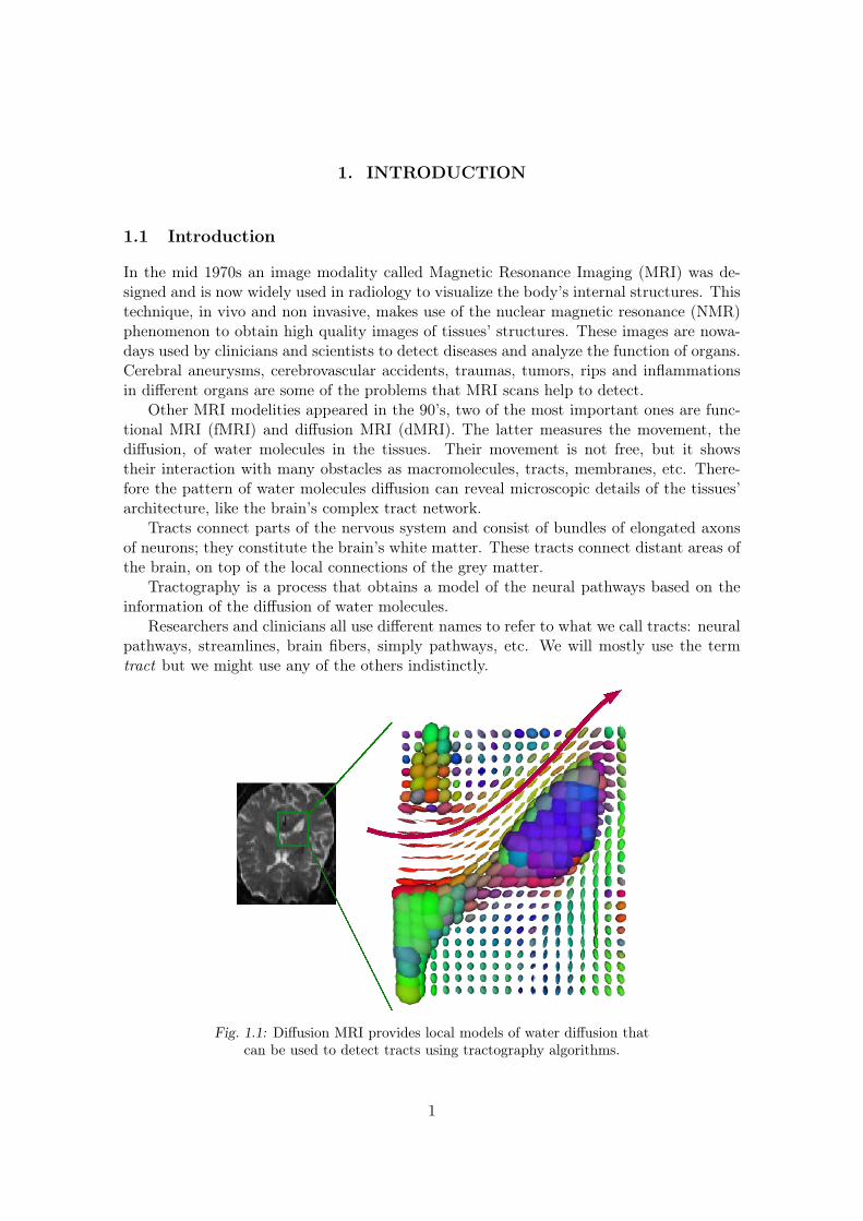
Tractography is a process that obtains a model of the neural pathways based on theinformation of the diffusion of water molecules.
Researchers and clinicians all use different names to refer to what we call tracts: neuralpathways, streamlines, brain fibers, simply pathways, etc. We will mostly use the termtract but we might use any of the others indistinctly.
Fig. 1.1: Diffusion MRI provides local models of water diffusion thatcan be used to detect tracts using tractography algorithms.
1
2 1. Introduction
Motivation
Tracts not only provide information about the connections between the different corticaland subcortical areas, but they are also used to detect certain anomalies (e.g. tumors), tocompare the brains of groups of patients (both diseased and healthy), etc. Scientists haverecently started to use them to improve registration algorithms applied to brain images[26, 35] (registering images means finding a common coordinate system that allows oneto consider that a certain point in one image corresponds to another point in the secondimage).
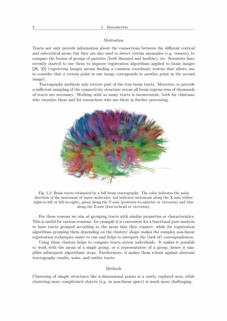
Tractography methods only recover part of the true brain tracts. Moreover, to providea sufficient sampling of the connectivity structure across all brain regions tens of thousandsof tracts are necessary. Working with so many tracts is inconvenient, both for clinicianswho visualize them and for researchers who use them in further processing.
Fig. 1.2: Brain tracts estimated by a full brain tractography. The color indicates the maindirection of the movement of water molecules: red indicates movement along the X-axis (eitherright-to-left or left-to-right), green along the Y-axis (posterior-to-anterior or viceversa) and blue
along the Z-axis (foot-to-head or viceversa).
For these reasons we aim at grouping tracts with similar properties or characteristics.This is useful for various reasions: for example it is convenient for a functional post-analysisto have tracts grouped according to the areas that they connect, while for registrationalgorithms grouping them depending on the clusters’ shape makes the complex non-linearregistration techniques easier to run and helps to interpret the (lack of) correspondences.
Using these clusters helps to compare tracts across individuals. It makes it possibleto work with the mean of a single group, or a representative of a group, hence it sim-plifes subsequent algorithmic steps. Furthermore, it makes them robust against aberranttractography results, noise, and outlier tracts.
Methods
Clustering of simple structures like n-dimensional points is a vastly explored area, whileclustering more complicated objects (e.g. in non-linear space) is much more challenging.
1.1. Introduction 3
The main problem that we face is to define a relevant metric to assess the similarity oftracts. Another one is to pick the right number of classes, which is a very hard problemin general as we are in an unsupervised setting. We will not try to solve this issue inparticular in this thesis.
We will approach the problem firstly by using known algorithms which have been provento give good results like K-Means and DBSCAN [5]. Different other approaches have beenproposed in the literature [30, 14, 31, 2, 32, 35, 11, 13, 33, 18] and yield alternative solutions.
These algorithms take as an input either n-dimensional points or distance matrices,therefore what matters are not the objects themselves but the distances between them. Wecall metric the function that quantifies the distance between tracts. Metric specificationentails some trade-offs: one can opt for a fast metric (in terms of computational cost),or one that helps maintain the geometric shape of the cluster’s tracts, or one which seekto keep the cluster compact, etc. One can also use atlases to group tracts in well-knownbundles. Some approaches are the Euclidian and Hausdorff distances, Mean Closest Point,Currents [4], Point Density Model [17], and Gaussian Processes [32].
We will evaluate the implications of choosing a given metric and how it combines withthe different algorithms, which will in turn be analyzed regarding speed and suitability tothe task. The scalability of both the clustering algorithm and the metrics, although notcritical for our needs, will also be taken into account.
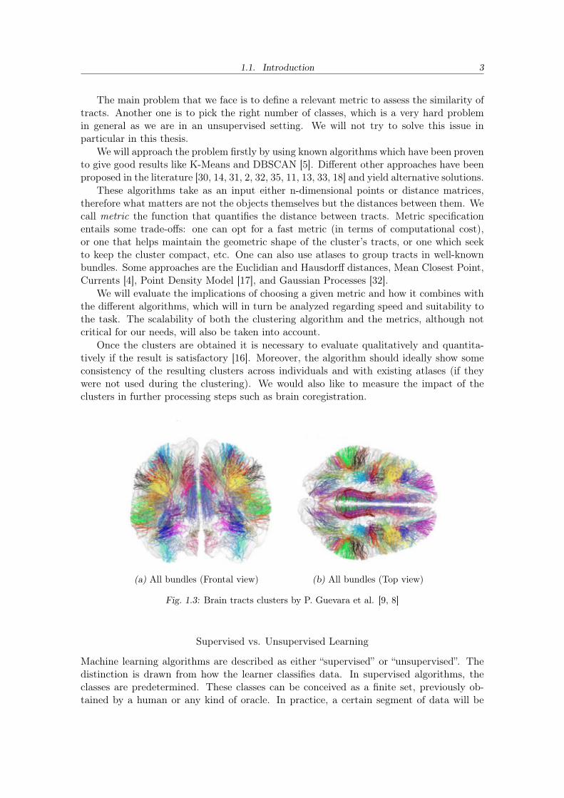
Once the clusters are obtained it is necessary to evaluate qualitatively and quantita-tively if the result is satisfactory [16]. Moreover, the algorithm should ideally show someconsistency of the resulting clusters across individuals and with existing atlases (if theywere not used during the clustering). We would also like to measure the impact of theclusters in further processing steps such as brain coregistration.
(a) All bundles (Frontal view) (b) All bundles (Top view)
Fig. 1.3: Brain tracts clusters by P. Guevara et al. [9, 8]
Supervised vs. Unsupervised Learning
Machine learning algorithms are described as either “supervised” or “unsupervised”. Thedistinction is drawn from how the learner classifies data. In supervised algorithms, theclasses are predetermined. These classes can be conceived as a finite set, previously ob-tained by a human or any kind of oracle. In practice, a certain segment of data will be

4 1. Introduction
labelled with these classifications. The machine learner’s task is to search for patterns andconstruct mathematical models. These models then are evaluated on the basis of their pre-dictive ability in relation to measures of variance in the data itself. Examples of supervisedlearning techniques are decision tree induction, naïve Bayes, etc..
Unsupervised learners are not provided with classifications. In fact, the basic taskof unsupervised learning is to develop classification labels automatically. Unsupervisedalgorithms seek out similarity between pieces of data in order to determine whether theycan be characterized as forming a group. These groups are termed clusters, and there area whole family of clustering machine learning techniques.
In unsupervised classification, often known as “cluster analysis” the machine is not toldhow the items are grouped. Its task is to arrive at some grouping of the data. In Kmeans,one of the most common algorithms for cluster analysis, the machine is told in advancehow many clusters it should form – a potentially difficult and arbitrary decision to make.
It is apparent from this minimal account that the optimization step involved in un-supervised classification is somewhat ill-posed. Some initialization is taken more or lessarbitrarily and the learning algorithms reach iteratively a stable configuration that makessense. The results vary widely and may be completely off if the first steps are wrong. Onthe other hand, cluster analysis has great potential to reveal unexpected details of thedata. And it has considerable corroborative power if its internal comparisons of low-levelfeatures of the items lead to groupings that make sense at a higher interpretative level orthat one had suspected but deliberately withheld from the machine. Thus cluster analysisis a very promising tool for the exploration of relationships among groups.
2. METHODS
The core of this project is based on the scikit-learn [19], an open source machine learninglibrary for Python. The tractographies and its visualizations were done thanks to medInria[28], an open source medical image processing and visualization software: http://med.inria.fr/.
2.1 Metrics
A metric is a function that measures distances in a given space. Besides the well-knownEuclidean distances many other metrics have been invented to fulfil different needs. In thecase of tracts, lines in a 3D space, we consider the four metrics described hereafter.
Given two tracts represented as a sequence of points in a 3-dimensional space X ={x1, x2, ..., xnk} and Y = {y1, y2, ..., yyk} where xi, yj ∈ R3 ∀1 ≤ i ≤ xk, ∀1 ≤ j ≤ yk wedefine four candidate metrics in the next subsections.
Two of these metrics need us to resample tracts X and Y so they have the same amountof points each. We assume from now on that an initial discretization of tracts has beenapplied, so that all tracts have the same number of points K. This is a achieved by asimple linear interpolation. Tracts are now X = {x1, x2, ..., xk} and Y = {y1, y2, ..., yk}where xi, yj ∈ R3 ∀1 ≤ i, j ≤ k.
Hausdoff and Mean Closes Point are widely-used, well-known metrics, we explain themin Appendix A along with Minimum Direct Flip, the metric used by Garyfallidis et al [7]for QuickBundles.
Additionally, we introduce Point Density Model:
2.1.1 Point Density Model
We propose to use the Point Density Model (PDM) metric which has been used previouslyfor representing sulcal lines [1] but has never been used to measure inter-tract distances.
The oriented version of Point Density Model called Currents has been used to representtracts in a registration scheme in [25].
We propose the Point Density Model to better capture the tracts’ shape. PDM issensitive to the tracts’ form and position and is quite robust to missing tract segments.This last property is much desired as tracts are often mis-segmented due to noise andcrossing tracts issues.
Definition: Given a tract X, we represent it as the sum of Dirac concentrated at eachtract point: 1
k
∑ki=1 δxi (resp. Y ).
Let Kσ be a Gaussian kernel with scale parameter σ, we can conveniently define thescalar product between two tracts as follows:
〈X,Y 〉 =1
k2
k∑i=1
k∑j=1
Kσ(xi, yj)
The definition of the Gaussian Kernel K is:
5
6 2. Methods
K(p, q) = e−||p−q||2
2σ2
The Point Density Model distance is thus defined as:
PDM 2(X,Y ) = ‖X‖2 + ‖Y ‖2 − 2〈X,Y 〉
This distance captures misalignment and shape dissimilarities at the resolution σ. Dis-tances much larger or much smaller than σ do not influence the metric.
Point Density Model is O(n2): quadratic on the number of points per tract.
2.2 Clustering Algorithms
Clustering a data set in an unsupervised setting is a complex and well-known problem, itis actually NP-hard. However, there are efficient heuristic algorithms that are commonlyemployed and converge quickly to a local optimum.
In this thesis we will use the well-known K-means algorithm and one of its variants,Mini-Batch K-means which offers faster running times in exchange of small looses in clusterquality. We will also experiment with DBSCAN which is strong where K-means is weak.
Our proposed solution, explained in 2.5 uses K-means at its core. We’ll compare ourresults againts QuickBundle, a trac-oriented clustering algorithm proposed by Garyfallidiset al [7] in 2012.
An explanatino of these algorithms can be found in Appendix B.Ideally we would simply want to run these algorithms, using the metrics described in
section 2.1, on the tracts outputted by the tractography procedure. Unfortunately giventhe time-complexity of the resulting algorithm and the size of the input sets, this is unviableas a single run can take days.
In order to use both concepts in a reasonsable amount of time we combine them byusing a Multidimensional Scaling technique.
2.3 Multidimensional Scaling
To-do/Question: rewrite and remove the following items
• que es
• para que se usa
• para que lo usamos nosotros
• aclaracion: no reducimos dimensiones. podriamos haber probado eso. agregar aseccion future work.
Multidimensional Scaling is a technique that computes a coordinates matrix out of adistance matrix so that the the between-object distances are preserved as well as possible.The dimension of the generated objects is a parameter in the algorithm which meansthat the original objects that generated the distace matric, which could have been in an-dimensional space, can be reduced to a 2- or 3-dimensional space, which is very usefulfor plotting. For this reason MDS is a technique widely used in information visualizationand data analysis.
2.4. Combining MDS with metrics 7
2.3.1 Mathematical Definition
Adapted from the Wikipedia article on Multidimensional scaling http://en.wikipedia.org/wiki/Multidimensional_scaling#Details.
The data to be analyzed is a collection of F tracts on which a distance function isdefined. δi,j is the distance between the ith and jth tracts. These distances are the entriesof the distance matrix:
∆ =
δ1,1 δ1,2 · · · δ1,Iδ2,1 δ2,2 · · · δ2,I...
......
δI,1 δI,2 · · · δI,I
.
The goal of MDS is, given ∆, to find F ′ tract x1, . . . , xI ∈ RN such that
‖xi − xj‖ ≈ δi,j∀i, j ∈ Fwhere ‖ · ‖ is a vector norm. In classical MDS, this norm is the Euclidean distance,
but, in a broader sense, it may be a metric or arbitrary distance function, for instance wecould use the metrics described above.
In other words, MDS attempts to find an embedding from the F tracts into RN suchthat distances are preserved. The resulting vectors xi are not unique: with the Euclideandistance for instance, they may be arbitrarily translated, rotated, and reflected, since thesetransformations do not change the pairwise distances ‖xi − xj‖.
There are various approaches to determining the vectors xi. Usually, MDS is formu-lated as an optimization problem, where (x1, . . . , xI) is found as a minimizer of some costfunction, for example:
minx1,...,xI
∑i<j
(‖xi − xj‖ − δi,j)2.
A solution may then be found by numerical optimization techniques. For some par-ticularly chosen cost functions, minimizers can be stated analytically in terms of matrixeigendecompositions.
To sum up, thanks to MDS we can go from a distance matrix to a set of objects whoseEuclidean distances closely approximates the distances in the distance matrix. We willcombine this with the metrics introduced in section 2.1.
2.4 Combining MDS with metrics
The metrics described in section 2.1 better capture the distance between two tracts butthey have an enormous disadvantage: they are very costly computational-wise. PointDensity Model and Hausdorff for instance are quadratic on the number of points per tractk. If we want to compute all the pairwise distances for N tracts it would cost us O
(N2k2
).
Computing a full matrix of pairwise distances for a small set of 20 000 tracts using Hausdorffon a single-core machine takes about 5 and a half hours, if we double the amount of tractsto 40 000 then it takes about 21 hours.
In order to be able to use these metrics that are more suitable for neural pathways wedecided to combine them with MDS to maintain the algorithm whitin a reasonable runningtime while incorporating the information provided by the metrics.
8 2. Methods
The algorithm goes as follows: say we have a group F of n tracts f1, . . . , fn. Eachtract fi has already been resampled so it has a resolution of k (i.e. exactly k 3-dimensionalpoints each). We take a random sample S of p tracts from F and then we compute agiven distance d between all the tracts in S and F , creating a distance matrix M of size〈n, p〉. We then apply MDS to this matrix to obtain a new set F ′ of n tract-like points(i.e. points belonging to R3k). These new points will capture the original information ofthe distance between them, which is the information that will be use afterward by theclustering algorithm.
By using a random sample of p elements, where p << N , we decrease the complexity toO(Npk2
)which in turn decreases the running time in a significant amount. Note that as
a first approach we do not intend to reduce the dimension of the points, this is somethingwe wanted to explore but we unfortunately did not have the time during this project.
The analysis of the size of p so as to keep the best possible trade-off between speedgain and information loss is treated in section 4.2.2.
2.5 The Algorithm
Below is the pseudo-code of the full algorithm. The input parameters are:
• a set Forig of n′ tracts, each tract being a list of points in R3
• ff : tracts with length < ff will be discarded
• p: percentage of the random sample
• m: the metric that will be used
• c: the clustering algorithm
1: F ←remove tracts shorter than ff mm from Forig2: resample every tract in F to exactly k points each3: S ← obtain random sample of F taking p% of the tracts4: M ← compute full distance matrix of tracts from S to F using metric m5: F ′ ← apply multi dimensional scaling, keep the same dimension = 3k6: C ← cluster F ′ with algorithm c (using Euclidean distance)7: return C
The innovative part of this algorithm lies in steps 4, 5 and 6. With MDS we obtain a newset of transformed samples F ′ which maps 1-to-1 to the original set F and approximatelypreserves the input distances, therefore information from the costly tract metric. MDSstarts with a distance matrix and assigns a location to each tract in N-dimensional space(in our case, number of points wanted per tract times the dimension of the points, 3 aswe are in R3). Here we use it asymmetrically, using the classical Nyström’s approach forefficient dimension reduction [6].
We discard tracts that are shorter than ff for mainly two reasons, firstly because theyare probably outliers of the tractography. Secondly because we do not aim at clusteringevery single tract in the output of a tractography, but rather to have bundles that makesense and help to understand the underlying structure at a glance. By leaving aside small,short tracts, the quality of the clusters increase.
2.5. The Algorithm 9
Both QB and Kmeans+metric running times are sensitive to the number of clusters,however QuickBundles’ time complexity is O(NCk) and Kmeans+metric O(NSk2+NCk),where C is the number of clusters, k the tract resolution and S the sample size. In thisalgorithm, the creation of the partial distance matrix dominates the time complexity aslong as Sk > C.

10 2. Methods
3. VALIDATION SCHEME
Evaluating the performance of a clustering algorithm is not as trivial as counting thenumber of errors or the precision and recall of a supervised classification algorithm. Inparticular any evaluation metric should not take the absolute values of the cluster labelsinto account but rather if this clustering define separations of the data similar to someground truth set of classes or satisfying some assumption such that members belong to thesame class are more similar that members of different classes according to some similaritymetric.
The problem of evaluating models in unsupervised settings is notoriously difficult. Herewe consider a set of standard criteria: the inertia of the clusters, the silhouette coefficientand some measures that require a ground truth: completeness, homogeneity, rand indexand its variants and mutual information and its variants.
3.1 Unsupervised Setting Scores
As we expained before, the most complicated scenario is when we do not have the realbundles to compare our clusters with. Unfortunately this is also the most common scenario.Below we explain the Inertia and the Silhouette scores, which makes it possible to rateclustering results under an unsupervised setting.
The most famous unsupervised score is the Inertia (explained in appendix C) but we’llbe using mostly the Silhouette Coefficient.
3.1.1 Silhouette Coefficient
The Silhouette Coefficient [22] measures how close a tract is to its own cluster in comparisonto the rest of the clusters, i.e. whether there is another cluster that might represent it betteror as well.
The silhouette score for a given tract is defined as:
silhouette =b− a
max(a, b)
where a is the mean intra-cluster distance (the mean distance between a sample and allother points in the same class) and b the mean nearest-cluster distance (the mean distancebetween a sample and all other points in the next nearest cluster).
The best value is 1 and the worst value is -1. Values near 0 indicate overlapping clusters.Negative values generally indicate that a sample has been assigned to the wrong cluster,as a different cluster is more similar.
The big drawback of this score is that an exact computation of it will require thecalculation of a full distance matrix (in order to find the nearest cluster) which rendersit prohibitive for our use. Using multi-dimensional scaling (MDS) method once againreduces the computation of the distances by approximating. We take a random sample sof the full tract set S and the labeling l and compute a partial distance matrix D of size〈S × s〉 and we use that to approximate the silhouette score. With 10% of the tracts, therelative error between the silhouette scores computed using the full distance matrix andthe approximated one was smaller than 10−2 on a random tract set (see section 4.2.2).
11
12 3. Validation Scheme
3.2 Supervised Setting Scores
Given a set F = {f1, . . . , fn} ofN tracts, the knowledge of the ground truth classes/bundles,i.e. a partition B = {B1, . . . , Br} of the original set of tracts F and our clustering algorithmassignments, another partition of F , C = {C1, . . . , Cs} a handful of scores that describehow similar both partitions are can be defined.
There are many scores for supervised settings, we’ll be using the Rand Index and it’s ad-justed for chance version the Adjusted Rand Index (ARI). Correctness, Completeness, andV-measure. The Normalized ARI and the Weighted Normalized ARI, two modificationsof the ARI by Moberts et al [16] specific for clusterings of brain tracts. And the MutualInformation score, and its adjusted for change version the Adjusted Mutual InformationScore. The definition of all these scores can be found in appendix C.
4. EXPERIMENTS AND RESULTS
4.1 Section Outline
In this chapter we will present the experiments we performed and the conclusions wedrafted out of them.
1. Point Density Model metric has a free parameter σ, it’s resolution. We will fix it insection 4.2.1.
2. Our algorithm, presented in section 2.5, has also a free parameter p: the size of therandom sample. It impacts the quality of the output clusters and the running timeof the algorithm. We’ll explore it’s impact in section 4.2.2 and we will fix it for allour experiments.
3. The first step when experimenting with problems whose solution is unknown is to runthe candidate algorithms on a reduced dataset, one where the solution is known, i.e.a selection of fibers whose original clusterization is defined beforehand by us, hence a“Manually Labelled Dataset”. As with this data set the expected clusterization, thesolution, is known, we’ll be able to use the scores for supervised settings scores weexplained in section 3.2. We will also see if the results provided by these scores arealigned with the ones provided by the Silhouette Coefficient, the score we will usewhen running the algorithm of a full brain tractography, therefore on an unsupervisedsetting.
4. DBSCAN: we ran DBSCAN first on the manually labelled dataset and then on fulltractographies. We present the results and draft conclusions in section 4.4.
5. Mini Batch K-means is known to be siginificantly faster than K-means while generat-ing clusters which are slightly worse. We ran experiments to determine whether thisis also the case in our domain, clustering of brain tracts. Conclusions are presentedin section 4.5.
6. Finally we run the algorithm we proposed in section 2.5, first on the manually labelleddataset introduced in section 4.3 and then on full tractographies with thousands oftracts.
4.2 Parameter Exploration
Our algorithm, described in section 2.5, has 2 free paramaters: p, the size of the randomsample used by MDS, and σ, the resolution of Point Density Model metric. We’ll analysetheir impact in this section.
4.2.1 Sigma: PDM Kernel Resolution
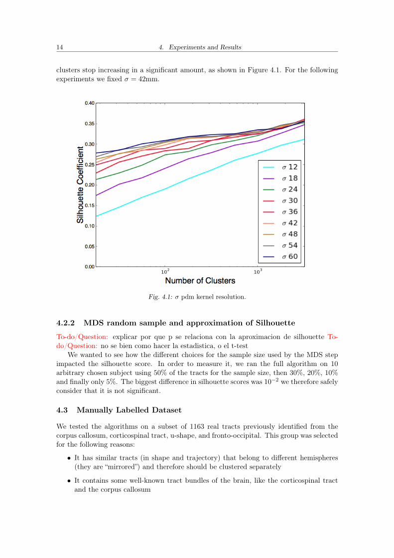
We performed a parameter selection test over 10 subject to analyze the impact of thekernel size for K-means with Point Density Model. We vary σ from 10 to 60mm and thenumber of clusters from 200 to 1200. We noticed that after σ = 42mm the quality of the
13
14 4. Experiments and Results
clusters stop increasing in a significant amount, as shown in Figure 4.1. For the followingexperiments we fixed σ = 42mm.
Fig. 4.1: σ pdm kernel resolution.
4.2.2 MDS random sample and approximation of Silhouette
To-do/Question: explicar por que p se relaciona con la aproximacion de silhouette To-do/Question: no se bien como hacer la estadistica, o el t-test
We wanted to see how the different choices for the sample size used by the MDS stepimpacted the silhouette score. In order to measure it, we ran the full algorithm on 10arbitrary chosen subject using 50% of the tracts for the sample size, then 30%, 20%, 10%and finally only 5%. The biggest difference in silhouette scores was 10−2 we therefore safelyconsider that it is not significant.
4.3 Manually Labelled Dataset
We tested the algorithms on a subset of 1163 real tracts previously identified from thecorpus callosum, corticospinal tract, u-shape, and fronto-occipital. This group was selectedfor the following reasons:
• It has similar tracts (in shape and trajectory) that belong to different hemispheres(they are “mirrored”) and therefore should be clustered separately
• It contains some well-known tract bundles of the brain, like the corticospinal tractand the corpus callosum
4.4. DBSCAN experiments and results 15
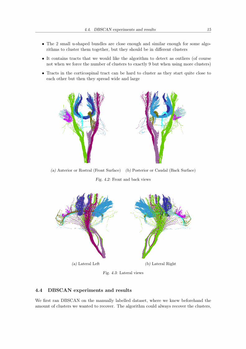
• The 2 small u-shaped bundles are close enough and similar enough for some algo-rithms to cluster them together, but they should be in different clusters
• It contains tracts that we would like the algorithm to detect as outliers (of coursenot when we force the number of clusters to exactly 9 but when using more clusters)
• Tracts in the corticospinal tract can be hard to cluster as they start quite close toeach other but then they spread wide and large
(a) Anterior or Rostral (Front Surface) (b) Posterior or Caudal (Back Surface)
Fig. 4.2: Front and back views
(a) Lateral Left (b) Lateral Right
Fig. 4.3: Lateral views
4.4 DBSCAN experiments and results
We first ran DBSCAN on the manually labelled dataset, where we knew beforehand theamount of clusters we wanted to recover. The algorithm could always recover the clusters,
16 4. Experiments and Results
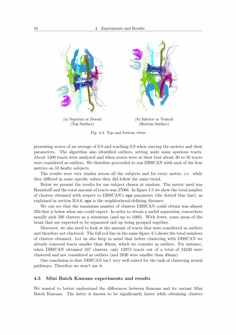
(a) Superior or Dorsal(Top Surface)
(b) Inferior or Ventral(Bottom Surface)
Fig. 4.4: Top and bottom views
presenting scores of an average of 0.8 and reaching 0.9 when varying the metrics and theirparameters. The algorithm also identified outliers, setting aside some spurious tracts.About 1200 tracts were analyzed and when scores were at their best about 30 to 50 tractswere considered as outliers. We therefore proceeded to run DBSCAN with each of the fourmetrics on 10 healty subjects.
The results were very similar across all the subjects and for every metric, i.e. whilethey differed in some specific values they did follow the same trend.
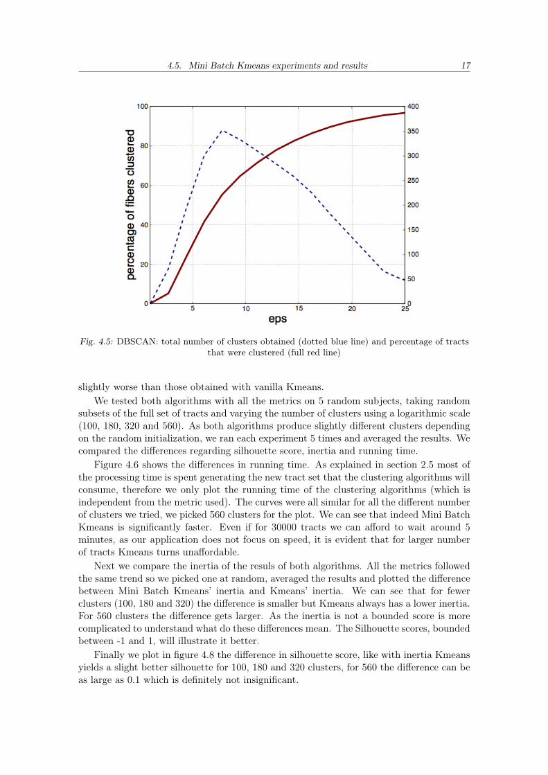
Below we present the results for one subject chosen at random. The metric used wasHausdorff and the total amount of tracts was 27066. In figure 4.5 we show the total numberof clusters obtained with respect to DBSCAN’s eps parameter (the dotted blue line); asexplained in section B.0.6, eps is the neighborhood-defining distance.
We can see that the maximum number of clusters DBSCAN could obtain was almost350 that is below what one could expect. In order to obtain a useful separation, researchersusually pick 500 clusters as a minimum (and up to 1000). With fewer, some areas of thebrain that are expected to be separated end up being grouped together.
Moreover, we also need to look at the amount of tracts that were considered as outliersand therefore not clustered. The full red line in the same figure 4.5 shows the total numbersof clusters obtained. Let us also keep in mind that before clustering with DBSCAN wealready removed tracts smaller than 40mm, which we consider as outliers. For instance,when DBSCAN obtained 347 clusters, only 12974 tracts out of a total of 24240 wereclustered and not considered as outliers (and 2826 were smaller than 40mm).
Our conclusion is that DBSCAN isn’t very well suited for the task of clustering neuralpathways. Therefore we won’t use it.
4.5 Mini Batch Kmeans experiments and results
We wanted to better understand the differences between Kmeans and its variant MiniBatch Kmeans. The latter is known to be significantly faster while obtaining clusters
4.5. Mini Batch Kmeans experiments and results 17
Fig. 4.5: DBSCAN: total number of clusters obtained (dotted blue line) and percentage of tractsthat were clustered (full red line)
slightly worse than those obtained with vanilla Kmeans.We tested both algorithms with all the metrics on 5 random subjects, taking random
subsets of the full set of tracts and varying the number of clusters using a logarithmic scale(100, 180, 320 and 560). As both algorithms produce slightly different clusters dependingon the random initialization, we ran each experiment 5 times and averaged the results. Wecompared the differences regarding silhouette score, inertia and running time.
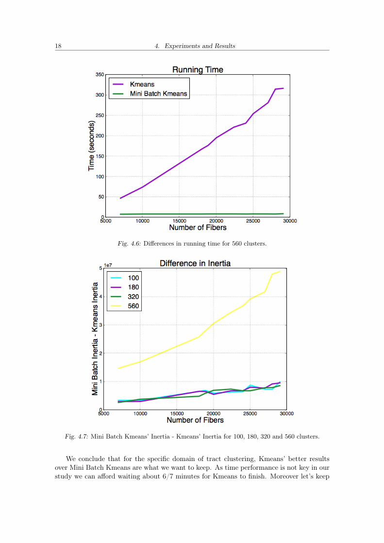
Figure 4.6 shows the differences in running time. As explained in section 2.5 most ofthe processing time is spent generating the new tract set that the clustering algorithms willconsume, therefore we only plot the running time of the clustering algorithms (which isindependent from the metric used). The curves were all similar for all the different numberof clusters we tried, we picked 560 clusters for the plot. We can see that indeed Mini BatchKmeans is significantly faster. Even if for 30000 tracts we can afford to wait around 5minutes, as our application does not focus on speed, it is evident that for larger numberof tracts Kmeans turns unaffordable.
Next we compare the inertia of the resuls of both algorithms. All the metrics followedthe same trend so we picked one at random, averaged the results and plotted the differencebetween Mini Batch Kmeans’ inertia and Kmeans’ inertia. We can see that for fewerclusters (100, 180 and 320) the difference is smaller but Kmeans always has a lower inertia.For 560 clusters the difference gets larger. As the inertia is not a bounded score is morecomplicated to understand what do these differences mean. The Silhouette scores, boundedbetween -1 and 1, will illustrate it better.
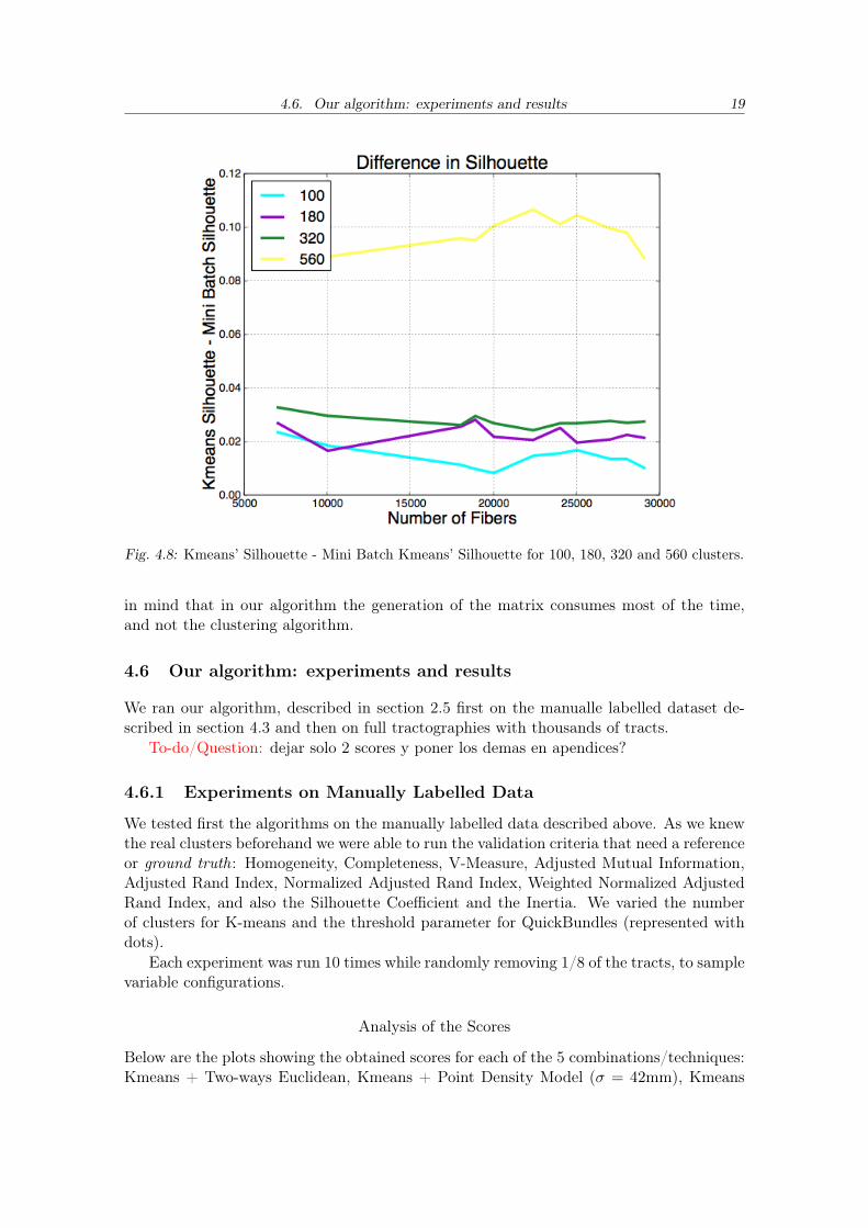
Finally we plot in figure 4.8 the difference in silhouette score, like with inertia Kmeansyields a slight better silhouette for 100, 180 and 320 clusters, for 560 the difference can beas large as 0.1 which is definitely not insignificant.
18 4. Experiments and Results
Fig. 4.6: Differences in running time for 560 clusters.
Fig. 4.7: Mini Batch Kmeans’ Inertia - Kmeans’ Inertia for 100, 180, 320 and 560 clusters.
We conclude that for the specific domain of tract clustering, Kmeans’ better resultsover Mini Batch Kmeans are what we want to keep. As time performance is not key in ourstudy we can afford waiting about 6/7 minutes for Kmeans to finish. Moreover let’s keep
4.6. Our algorithm: experiments and results 19
Fig. 4.8: Kmeans’ Silhouette - Mini Batch Kmeans’ Silhouette for 100, 180, 320 and 560 clusters.
in mind that in our algorithm the generation of the matrix consumes most of the time,and not the clustering algorithm.
4.6 Our algorithm: experiments and results
We ran our algorithm, described in section 2.5 first on the manualle labelled dataset de-scribed in section 4.3 and then on full tractographies with thousands of tracts.
To-do/Question: dejar solo 2 scores y poner los demas en apendices?
4.6.1 Experiments on Manually Labelled Data
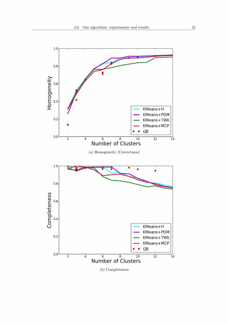
We tested first the algorithms on the manually labelled data described above. As we knewthe real clusters beforehand we were able to run the validation criteria that need a referenceor ground truth: Homogeneity, Completeness, V-Measure, Adjusted Mutual Information,Adjusted Rand Index, Normalized Adjusted Rand Index, Weighted Normalized AdjustedRand Index, and also the Silhouette Coefficient and the Inertia. We varied the numberof clusters for K-means and the threshold parameter for QuickBundles (represented withdots).
Each experiment was run 10 times while randomly removing 1/8 of the tracts, to samplevariable configurations.
Analysis of the Scores
Below are the plots showing the obtained scores for each of the 5 combinations/techniques:Kmeans + Two-ways Euclidean, Kmeans + Point Density Model (σ = 42mm), Kmeans

20 4. Experiments and Results
+ Mean Closest Point, Kmeans + Hausdorff, and QuickBundles. An analysis is presentedafterward.
4.6. Our algorithm: experiments and results 21
(a) Homogeneity (Correctness)
(b) Completeness
22 4. Experiments and Results
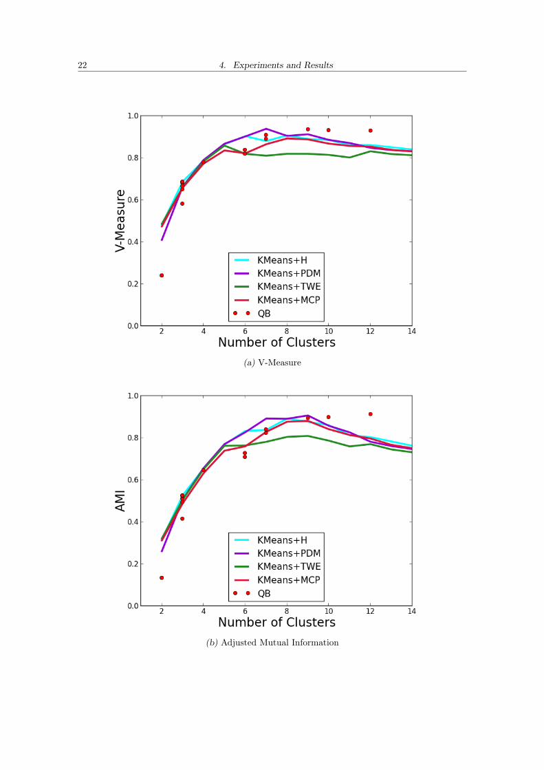
(a) V-Measure
(b) Adjusted Mutual Information
4.6. Our algorithm: experiments and results 23
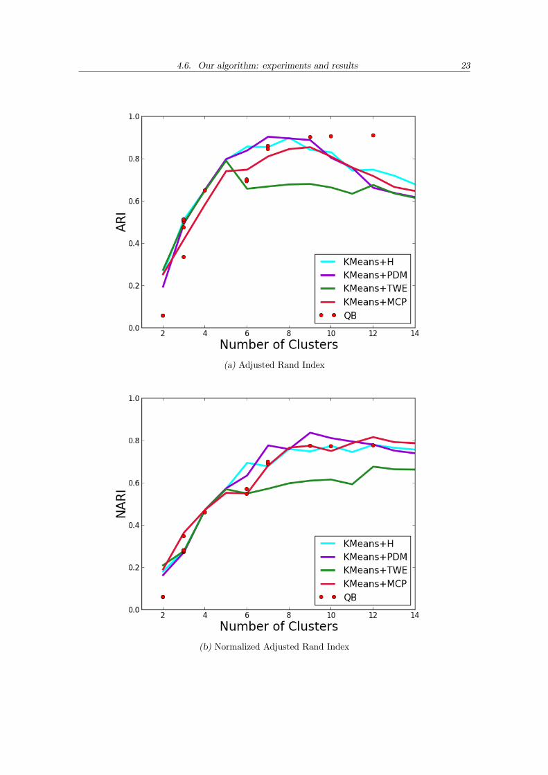
(a) Adjusted Rand Index
(b) Normalized Adjusted Rand Index
24 4. Experiments and Results
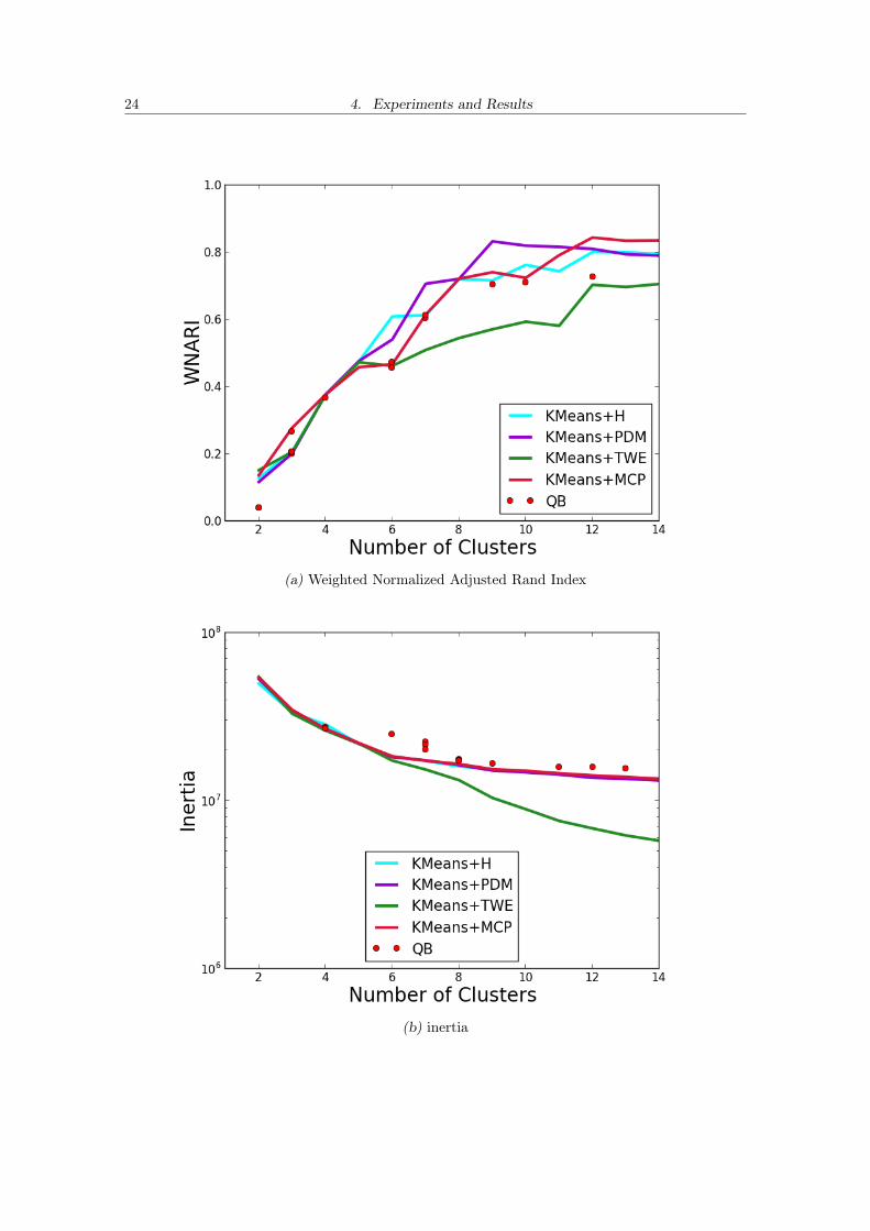
(a) Weighted Normalized Adjusted Rand Index
(b) inertia
4.6. Our algorithm: experiments and results 25
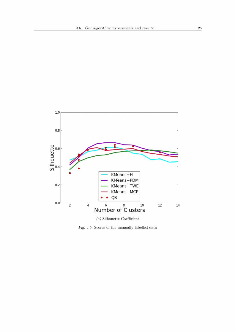
(a) Silhouette Coefficient
Fig. 4.5: Scores of the manually labelled data
26 4. Experiments and Results
First one can observe the scores that need a ground truth, i.e. all but Inertia andSilhouette. The closer they are to 1 the more similar the obtained clusters are to our 9manually labelled bundles, described in section 4.3.
The first three plots show the Correctness (Homogeneity), Completeness and V-Measure.As explained in section C.4, homogeneity penalizes the clustering scheme in which samplesfrom different classes are clustered together and Completeness the ones in which samplesfrom the same class are clustered separately, V-measure is the harmonic mean of both.If we only look at the V-measure we observe that for the desired amount of clusters, be-tween 8 and 10, QuickBundles behaves slightly better. By breaking it into Correctness andCompleteness we can see that QuickBundles behaves extremely well regarding complete-ness but not so well on homogeneity. On the other hand, KMeans+PDM obtained highhomogeneity but lower completeness, indicating that clusters contain tracts from the samestructure but that they are not complete, which means that some structures can be split.As we have explained in section C.6 this produces clusters of a lower quality.
The Adjusted Mutual Information and Adjusted Rand Index present similar graphs:up to 9 clusters KMeans+PDM clearly obtains higher scores but for larger numbers Quick-Bundles obtains clusters that are more similar to the ground truth. Again, as explainedin section C.6 these scores are very general and, while useful, don’t necessarily agree withclinicians’ opinions.
The Normalized ARI and the Weighted ARI are more adequate for our domain, theformer giving all bundles the same weight independently of the amount of tracts theycontain and the latter also giving more importance to clusters’ correctness over complete-ness. Their plots show that QuickBundles behaves quite poorly and Kmeans combinedwith PDM or MCP perform best. This also makes us wonder about the distribution of thetracts among the many clusters: it seems that QuickBundles is yielding some big clusters.We will analyse it later in section 4.6.2.
In order to be able to compare the algorithms and metrics using the inertia criterionwe decided to compute it, for all cases, using the Euclidean distance. This is why TWEpresents the lowest inertia score, Kmeans aims at minimizing the clusters’ inertia computedalso using the euclidean distances and TWE is very similar to it. By looking at the plot,we can effectively confirm that QuickBundles’ clusters have a higher variance than Kmeanscombined with the other metrics.
Lastly, the Silhouette scores puts Kmeans+PDM as the clear winner when below 11clusters and then TWE shows some advantage.
On average it can be observed that Kmeans with Point Density Model metric obtainsgood results for all cases. This was expected and reinforced by these experiments, as we be-lieve that this metric better captures the distance between tracts, taking into considerationdisaligments and shape dissimilarities.
Analysis of the Clusters
Below we present the clusters recovered by Kmeans when setting the number of clusterto 9 and by QuickBundles when settings the threshold parameter to 29.2mm (produced 9clusters).
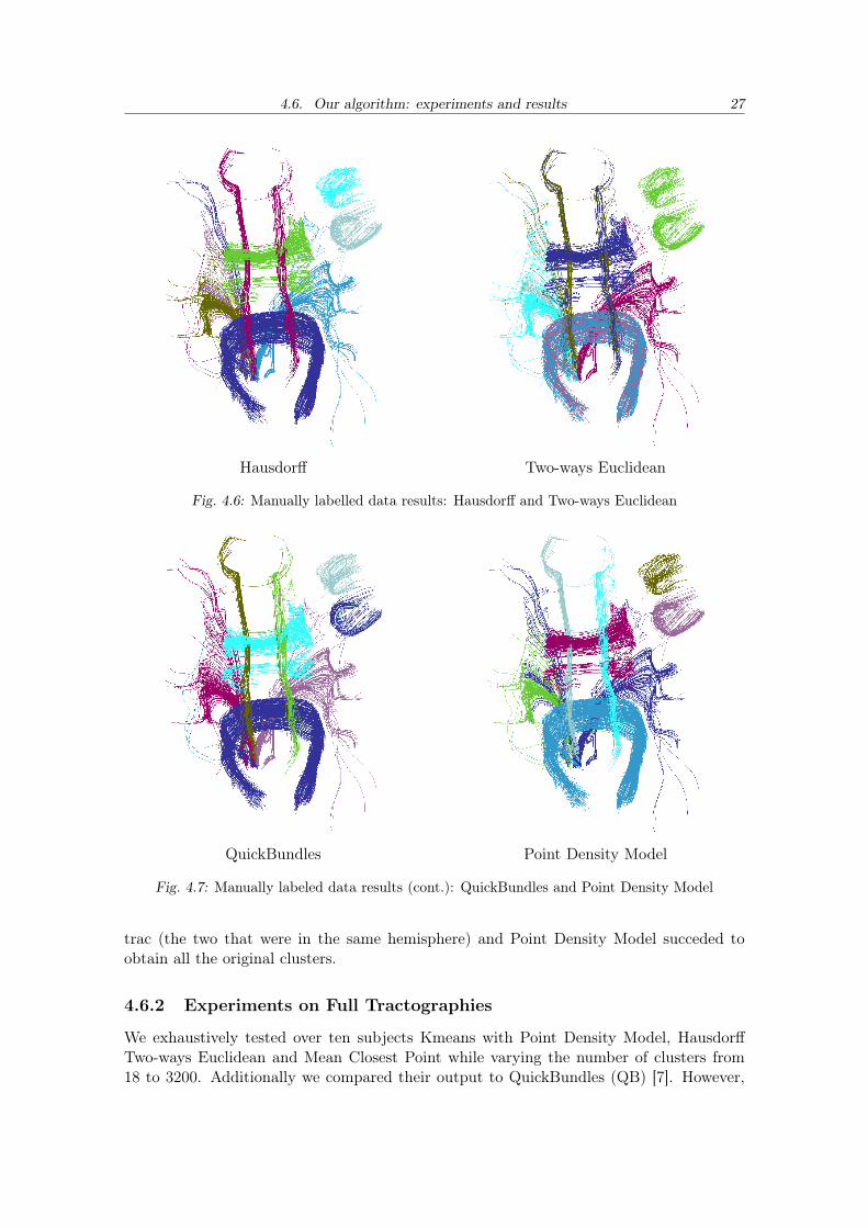
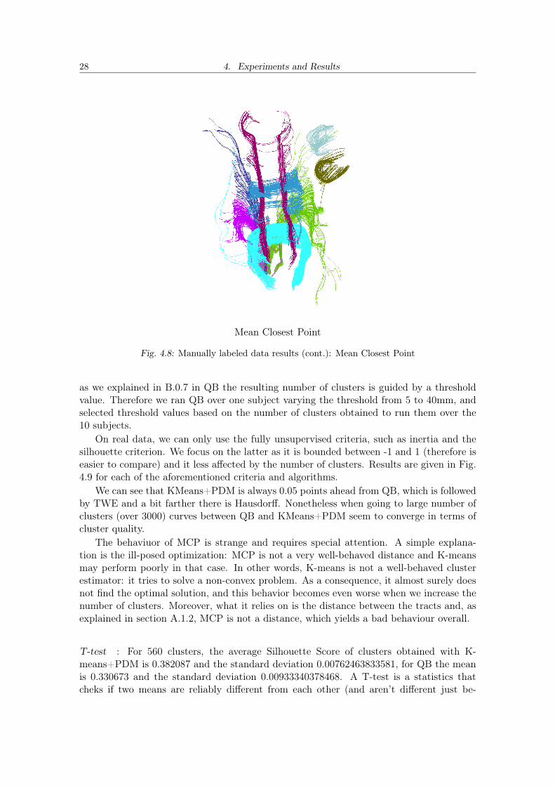
The 2 corpus callosum tract clusters were well identified by every algorithm exceptfor TWE which mixed some other tracts in too. The fronto-occipital tracts (the vertical,elongated ones) from both hemispheres were classified as a unique cluster for Hausdorff andMean Closest Point. Quickbundles mixed together 2 of the 3 bundles of the corticospinal
4.6. Our algorithm: experiments and results 27
Hausdorff Two-ways Euclidean
Fig. 4.6: Manually labelled data results: Hausdorff and Two-ways Euclidean
QuickBundles Point Density Model
Fig. 4.7: Manually labeled data results (cont.): QuickBundles and Point Density Model
trac (the two that were in the same hemisphere) and Point Density Model succeded toobtain all the original clusters.
4.6.2 Experiments on Full Tractographies
We exhaustively tested over ten subjects Kmeans with Point Density Model, HausdorffTwo-ways Euclidean and Mean Closest Point while varying the number of clusters from18 to 3200. Additionally we compared their output to QuickBundles (QB) [7]. However,
28 4. Experiments and Results
Mean Closest Point
Fig. 4.8: Manually labeled data results (cont.): Mean Closest Point
as we explained in B.0.7 in QB the resulting number of clusters is guided by a thresholdvalue. Therefore we ran QB over one subject varying the threshold from 5 to 40mm, andselected threshold values based on the number of clusters obtained to run them over the10 subjects.
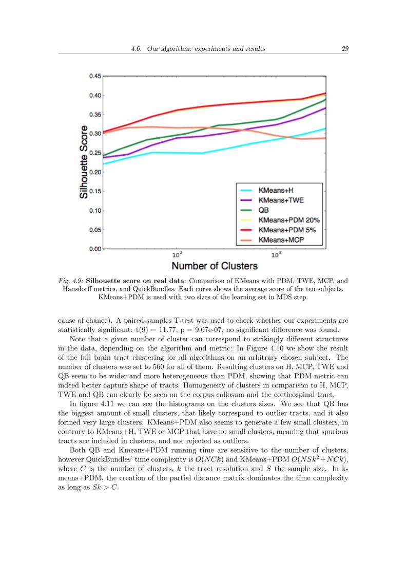
On real data, we can only use the fully unsupervised criteria, such as inertia and thesilhouette criterion. We focus on the latter as it is bounded between -1 and 1 (therefore iseasier to compare) and it less affected by the number of clusters. Results are given in Fig.4.9 for each of the aforementioned criteria and algorithms.
We can see that KMeans+PDM is always 0.05 points ahead from QB, which is followedby TWE and a bit farther there is Hausdorff. Nonetheless when going to large number ofclusters (over 3000) curves between QB and KMeans+PDM seem to converge in terms ofcluster quality.
The behaviuor of MCP is strange and requires special attention. A simple explana-tion is the ill-posed optimization: MCP is not a very well-behaved distance and K-meansmay perform poorly in that case. In other words, K-means is not a well-behaved clusterestimator: it tries to solve a non-convex problem. As a consequence, it almost surely doesnot find the optimal solution, and this behavior becomes even worse when we increase thenumber of clusters. Moreover, what it relies on is the distance between the tracts and, asexplained in section A.1.2, MCP is not a distance, which yields a bad behaviour overall.
T-test : For 560 clusters, the average Silhouette Score of clusters obtained with K-means+PDM is 0.382087 and the standard deviation 0.00762463833581, for QB the meanis 0.330673 and the standard deviation 0.00933340378468. A T-test is a statistics thatcheks if two means are reliably different from each other (and aren’t different just be-
4.6. Our algorithm: experiments and results 29
Fig. 4.9: Silhouette score on real data: Comparison of KMeans with PDM, TWE, MCP, andHausdorff metrics, and QuickBundles. Each curve shows the average score of the ten subjects.
KMeans+PDM is used with two sizes of the learning set in MDS step.
cause of chance). A paired-samples T-test was used to check whether our experiments arestatistically significant: t(9) = 11.77, p = 9.07e-07, no significant difference was found.
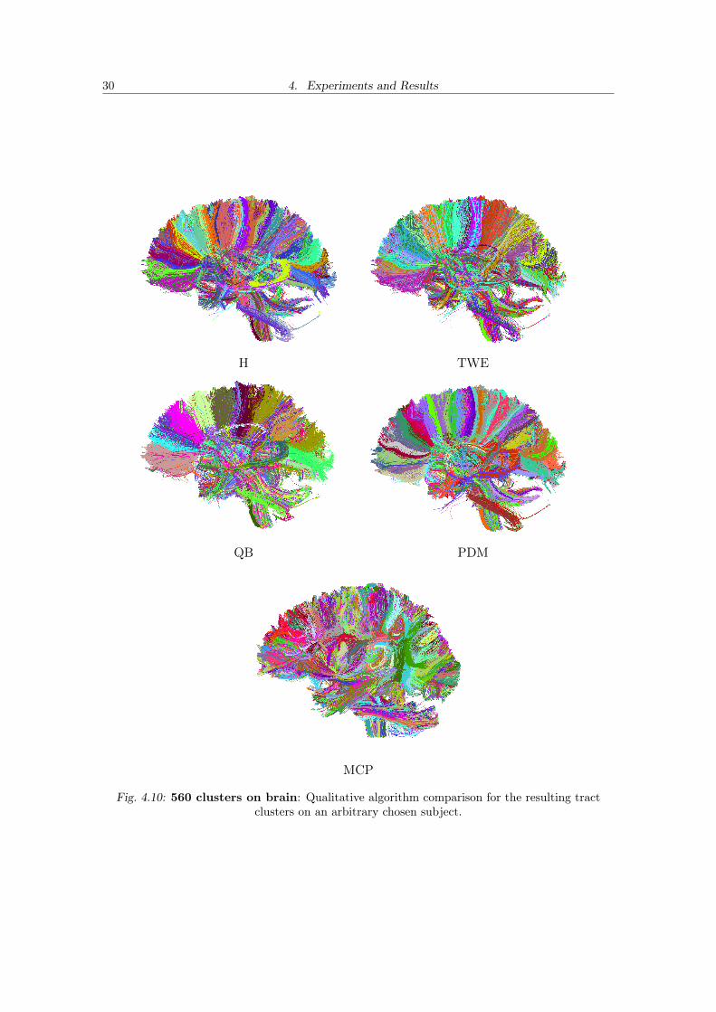
Note that a given number of cluster can correspond to strikingly different structuresin the data, depending on the algorithm and metric: In Figure 4.10 we show the resultof the full brain tract clustering for all algorithms on an arbitrary chosen subject. Thenumber of clusters was set to 560 for all of them. Resulting clusters on H, MCP, TWE andQB seem to be wider and more heterogeneous than PDM, showing that PDM metric canindeed better capture shape of tracts. Homogeneity of clusters in comparison to H, MCP,TWE and QB can clearly be seen on the corpus callosum and the corticospinal tract.
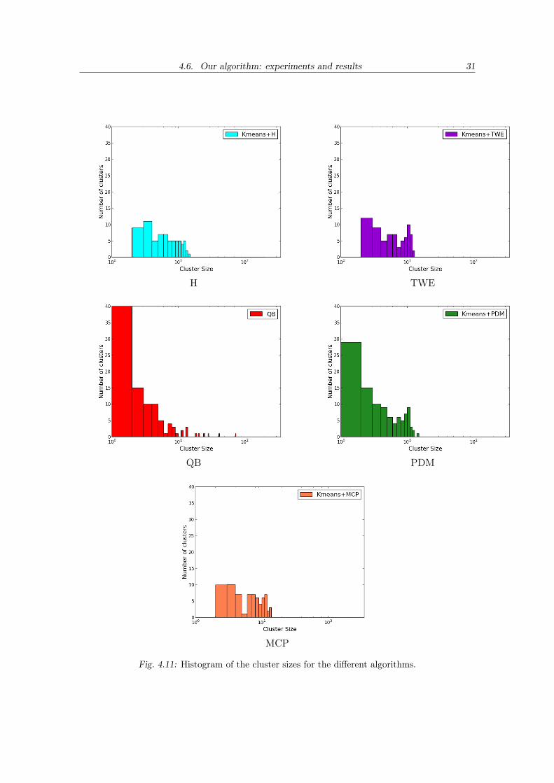
In figure 4.11 we can see the histograms on the clusters sizes. We see that QB hasthe biggest amount of small clusters, that likely correspond to outlier tracts, and it alsoformed very large clusters. KMeans+PDM also seems to generate a few small clusters, incontrary to KMeans+H, TWE or MCP that have no small clusters, meaning that spurioustracts are included in clusters, and not rejected as outliers.
Both QB and Kmeans+PDM running time are sensitive to the number of clusters,however QuickBundles’ time complexity is O(NCk) and KMeans+PDM O(NSk2+NCk),where C is the number of clusters, k the tract resolution and S the sample size. In k-means+PDM, the creation of the partial distance matrix dominates the time complexityas long as Sk > C.
30 4. Experiments and Results
H TWE
QB PDM
MCP
Fig. 4.10: 560 clusters on brain: Qualitative algorithm comparison for the resulting tractclusters on an arbitrary chosen subject.
4.6. Our algorithm: experiments and results 31
H TWE
QB PDM
MCP
Fig. 4.11: Histogram of the cluster sizes for the different algorithms.

32 4. Experiments and Results
5. CONCLUSIONS
We have presented an analysis and comparison of some of the techniques most commonlyused on tract clustering. Clustering is a tool of choice to simplify the complicated struc-ture of brain tracts, assuming that we obtain homogeneous clusters that can easily berepresented by the cluster centroid.
By introducing multi dimensional scaling techniques we could include and compare theavailable metrics on the literature for measuring distances between tracts, incorporatingPDM which has been used recently to represent geometric structures in the brain, butnever for tract clustering. We show different behaviors of the methods depending on thenumber of clusters: while QB is good at isolating outlier tracts in small clusters, it requiresa large number clusters to represent effectively the whole set of tracts. Kmeans+PDM hasa better compression power, but is less robust against outlier tracts. It clearly outperformsother metrics.
We believe that this method along with a posterior tract registration [25] can be aconsistent tool for white matter group analysis. In the future, it could be applied for theanalysis of white matter in neurological settings [3].
33

34 5. Conclusions
6. FUTURE WORK
During the development of this thesis we didn’t have the time to explore all the possibleoptions and to develop all the ideas that arose. Some particularly relevant questions toaddress further are:
• Test more metrics, like “Currents” [4], the oriented version of Point Density Model.This requires to somehow choose an orientation for each of the tracts, which is notan easy task. We also wanted to try using Gaussian Processes [32] which seemed tohave given good results to Wasserman et al. [32].
• Experiment with Brain Atlases to improve the clustering algorithms, a promisingoption, explored by Pamela Guevara et al [8].
• Measure the performance of Mini Batch Kmeans with huge tractographies andmillions of tracts, and compare it with QuickBundeles
• Explore reducing the dimension of the set obtained by MDS. What is the impact incluster quality and running time?
• Explore the impact of reducing the sample size below 5%. Does the cluster qualitydecrease significantly? How much is the speed gain?
35

36 6. Future Work

7. PUBLICATION
The paper version of this research A Comparison of Metrics and Algorithms for Fiber Clus-tering [24] has been published at the 3rd International Workshop on Pattern Recognition inNeuroImaging (PRNI) in June 2013, held at the University of Pennsylvania, Philadelphia,US (http://www.rad.upenn.edu/sbia/PRNI2013/).
37

38 7. Publication

Appendices
39

Appendix A
METRICS
A.1 Metrics
A.1.1 Hausdorff
From its Wikipedia article “Hausdorff Distance”: http://en.wikipedia.org/wiki/Hausdorff_distance.
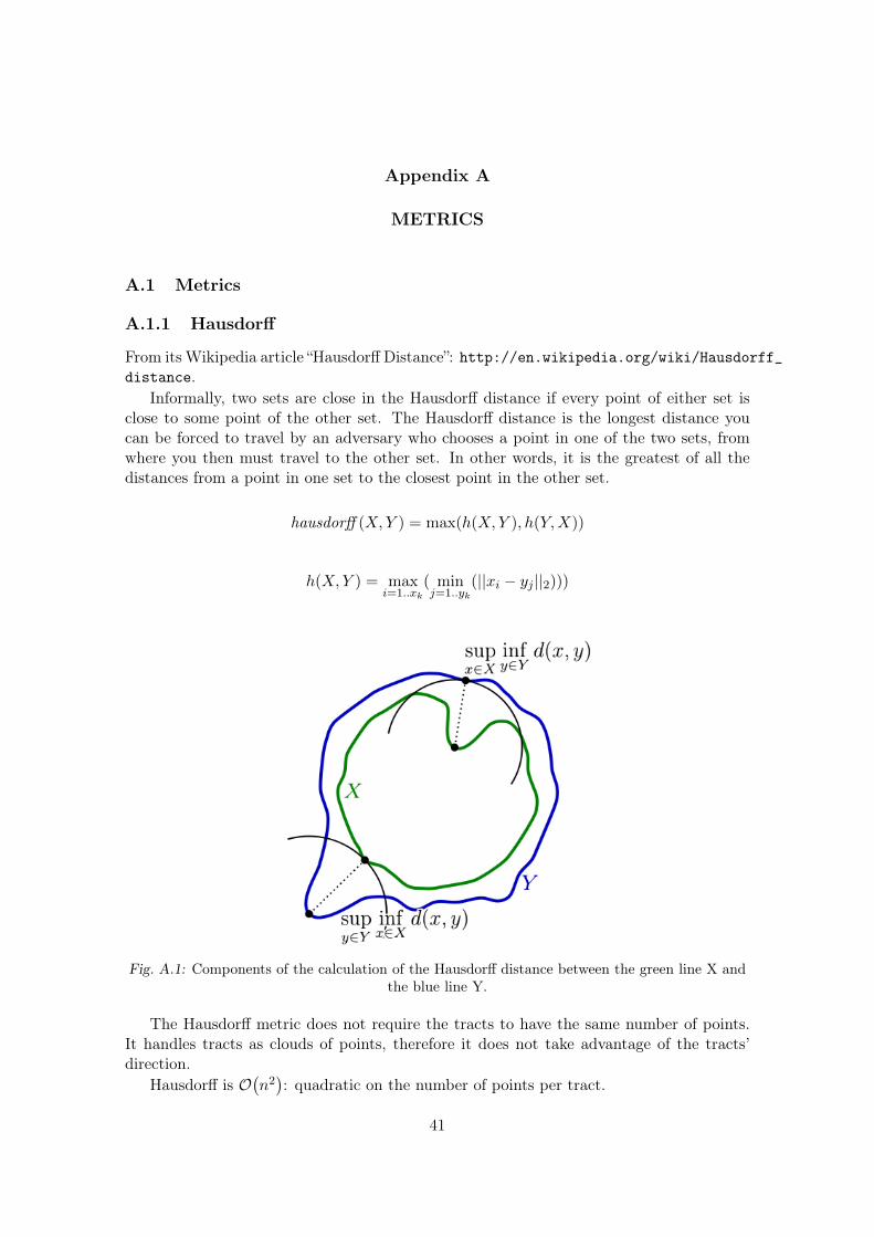
Informally, two sets are close in the Hausdorff distance if every point of either set isclose to some point of the other set. The Hausdorff distance is the longest distance youcan be forced to travel by an adversary who chooses a point in one of the two sets, fromwhere you then must travel to the other set. In other words, it is the greatest of all thedistances from a point in one set to the closest point in the other set.
hausdorff (X,Y ) = max(h(X,Y ), h(Y,X))
h(X,Y ) = maxi=1..xk
( minj=1..yk
(||xi − yj ||2)))
Fig. A.1: Components of the calculation of the Hausdorff distance between the green line X andthe blue line Y.
The Hausdorff metric does not require the tracts to have the same number of points.It handles tracts as clouds of points, therefore it does not take advantage of the tracts’direction.
Hausdorff is O(n2): quadratic on the number of points per tract.
41
42 Appendix A. Metrics
A.1.2 Mean Closest Point
Another common practice when measuring distances in the 3D space is taking a combina-tion of the distances of the closest points of the different subsets.
mcp =
∑xki=1 minj=1..yk ||xi − yj ||2
k+
∑ykj=1 mini=1..xk ||xi − yj ||2
k
MCP is O(n2): quadratic on the number of points per tract. Note that it is not a
metric, as it does not enforce the triangle inequality. This can lead to poor behavior inpractical applications.
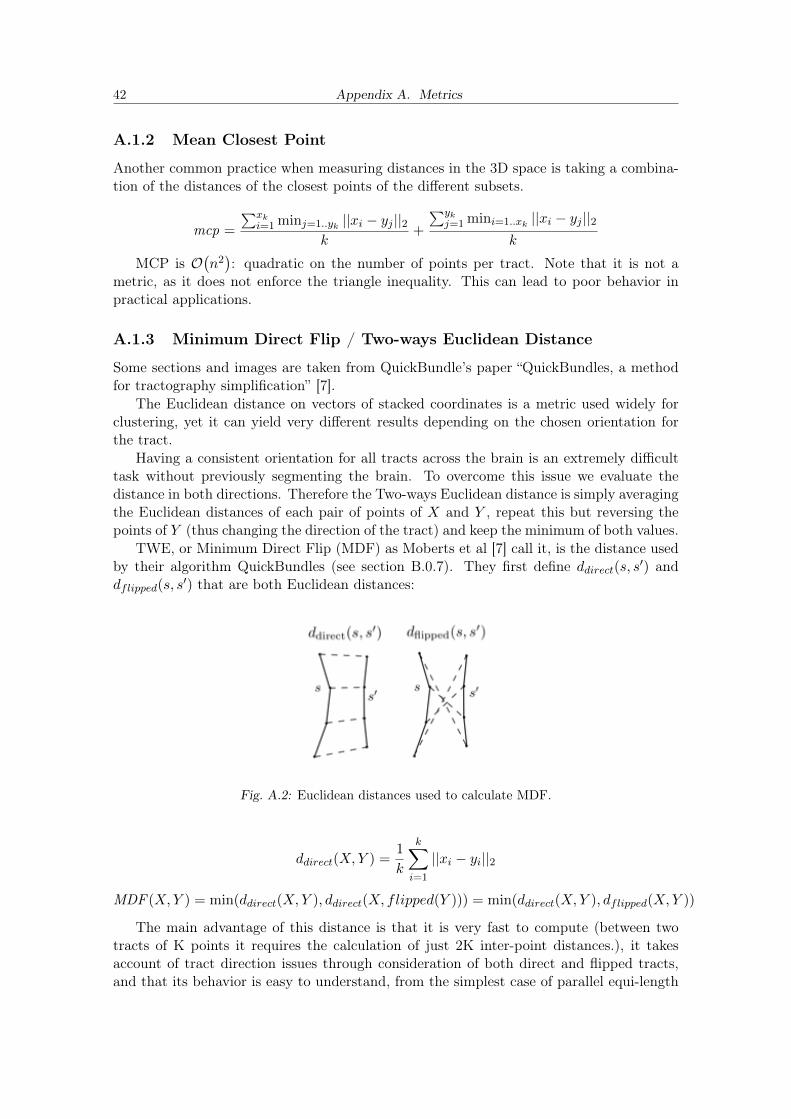
A.1.3 Minimum Direct Flip / Two-ways Euclidean Distance
Some sections and images are taken from QuickBundle’s paper “QuickBundles, a methodfor tractography simplification” [7].
The Euclidean distance on vectors of stacked coordinates is a metric used widely forclustering, yet it can yield very different results depending on the chosen orientation forthe tract.
Having a consistent orientation for all tracts across the brain is an extremely difficulttask without previously segmenting the brain. To overcome this issue we evaluate thedistance in both directions. Therefore the Two-ways Euclidean distance is simply averagingthe Euclidean distances of each pair of points of X and Y , repeat this but reversing thepoints of Y (thus changing the direction of the tract) and keep the minimum of both values.
TWE, or Minimum Direct Flip (MDF) as Moberts et al [7] call it, is the distance usedby their algorithm QuickBundles (see section B.0.7). They first define ddirect(s, s′) anddflipped(s, s
′) that are both Euclidean distances:
Fig. A.2: Euclidean distances used to calculate MDF.
ddirect(X,Y ) =1
k
k∑i=1
||xi − yi||2
MDF (X,Y ) = min(ddirect(X,Y ), ddirect(X, flipped(Y ))) = min(ddirect(X,Y ), dflipped(X,Y ))
The main advantage of this distance is that it is very fast to compute (between twotracts of K points it requires the calculation of just 2K inter-point distances.), it takesaccount of tract direction issues through consideration of both direct and flipped tracts,and that its behavior is easy to understand, from the simplest case of parallel equi-length
A.1. Metrics 43
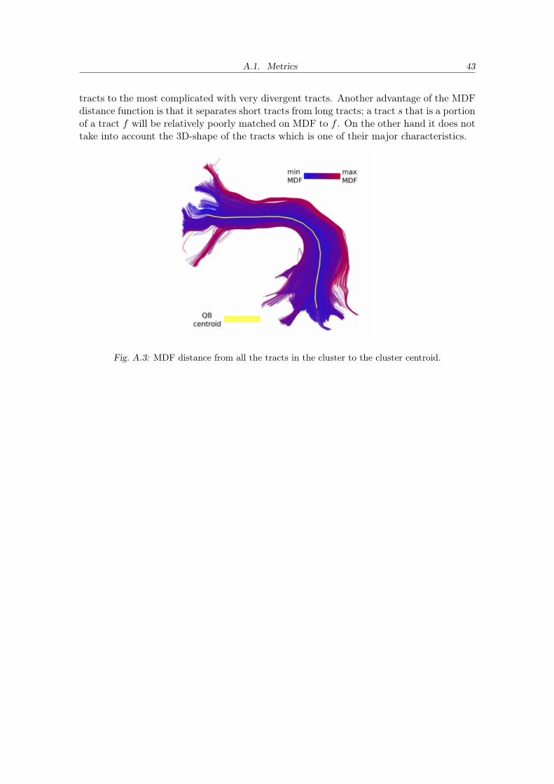
tracts to the most complicated with very divergent tracts. Another advantage of the MDFdistance function is that it separates short tracts from long tracts; a tract s that is a portionof a tract f will be relatively poorly matched on MDF to f . On the other hand it does nottake into account the 3D-shape of the tracts which is one of their major characteristics.
Fig. A.3: MDF distance from all the tracts in the cluster to the cluster centroid.

44 Appendix A. Metrics
Appendix B
ALGORITHMS
B.0.4 K-means
From Matteo Matteucci’s clustering tutorial: http://home.deib.polimi.it/matteucc/Clustering/tutorial_html/kmeans.html.
K-means clustering is a well-known method of cluster analysis which aims to partitionn observations into k clusters in which each observation belongs to the cluster with thenearest mean, where k is fixed a priori. This results in a partitioning of the data space intoVoronoi cells. Probably K-means is the most famous unsupervised learning algorithm thatsolves the well-known clustering problem. The term “K-means” was coined by MacQueenin 1967 [12] however the ideas goes back as far as 1956 with Hugo Steinhaus [27]. Thealgorithm was proposed also by S. Loyd and E. Forgy and this is why sometimes it isreferred as the Loyd-Forgy method in the computer science community. Hereafter we willrefer it simply as K-means.
The procedure follows a clear way to classify a given data set through k clusters fixed apriori. The main idea is to define k centroids, one for each cluster. These centroids shoudbe placed in a clever way because different placements cause different results. The nextstep is to take each point belonging to a given data set and associate it with the nearestcentroid. When no point is pending, the first step is completed and an early groupage isdone. At this point we need to recompute k new centroids as barycenters of the clustersresulting from the previous step. After we have these k new centroids, a new assignment ofthe data set points to the nearest centroid is done. This results in an update/assignmentloop. As a result of this loop we may notice that the k centroids change their location stepby step until no more changes are done. In other words centroids do not move any more.
The matemathical defitions is: given a set of observations (x1, . . . , xn), where eachobservation is a d-dimensional real vector, k-means clustering aims to partition the nobservations into k sets (k ≤ n) S = {S1, . . . , Sk} so as to minimize their inertia (thewithin-cluster sum of squares, see section C.1).
arg minS
k∑i=1
∑xj∈Si
‖xj − µi‖2
where µi is the cluster centroid, i.e. the mean of points in Si.
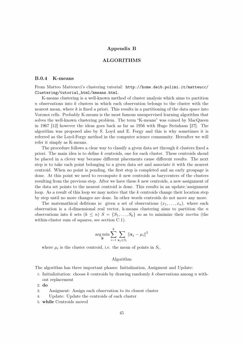
Algorithm
The algorithm has three important phases: Initialization, Assigment and Update:1: Initializitation: choose k centroids by drawing randomly k observations among n with-
out replacement2: do3: Assigment: Assign each observation to its closest cluster4: Update: Update the centroids of each cluster5: while Centroids moved
45
46 Appendix B. Algorithms
Initialization: Place k points m(1)1 , . . . ,m
(k)k into the space represented by the objects
that are being clustered. These points represent the initial group centroids.Assigment Step: Assign each observation to the cluster whose mean is closest to it
(i.e. partition the observations according to the Voronoi diagram generated by the means).
S(t)i =
{xp :
∥∥xp −m(t)i
∥∥ ≤ ∥∥xp −m(t)j
∥∥ ∀ 1 ≤ j ≤ k}
where each xp is assigned to exactly one S(t), even if it could be is assigned to two ormore of them.
Update step: Calculate the new means to be the centroids of the observations in thenew clusters.
m(t+1)i =
1
|S(t)i |
∑xj∈S
(t)i
xj
When the centroids ne longer move the algorithm has converged.
Analysis & Complexity
Although it can be proved that the procedure will always terminate, the k-means algorithmdoes not necessarily find the most optimal configuration, corresponding to the global objec-tive function minimum. The algorithm is actually sensitive to the initial randomly selectedcluster centres. The k-means algorithm can be run multiple times to reduce this effect.
The complexity of the algorithm is O(n×k× I×f), where n is the number of samples,k is the number of clusters we want, I is the number of iterations and f is the number offeatures in a particular sample. It can be clearly seen that the algorithm won’t scale forhuge number of objects to be clustered.
K-means is a simple algorithm that has been adapted to many problem domains. Inthis thesis we will adapt it to our specific needs.
B.0.5 Mini Batch K-means
From Scikit-learn’s Mini Batch K-means page http://scikit-learn.org/stable/modules/clustering.html#mini-batch-k-means and Siddharth Agrawal’s machine learning tuto-rial http://algorithmicthoughts.wordpress.com/2013/07/26/machine-learning-mini-batch-k-means/.
The Mini Batch K-Means [23] is a variant of the K-Means algorithm that uses mini-batches to drastically reduce the computation time, while still attempting to optimise thesame objective function. Mini-batches are subsets of the input data, randomly sampled ineach training iteration. These mini-batches drastically reduce the amount of computationrequired to converge to a local solution. In contrast to other algorithms that reduce theconvergence time of k-means, and depending on the domain, mini-batch k-means producesresults that are generally only slightly worse than the standard algorithm.
Algorithm
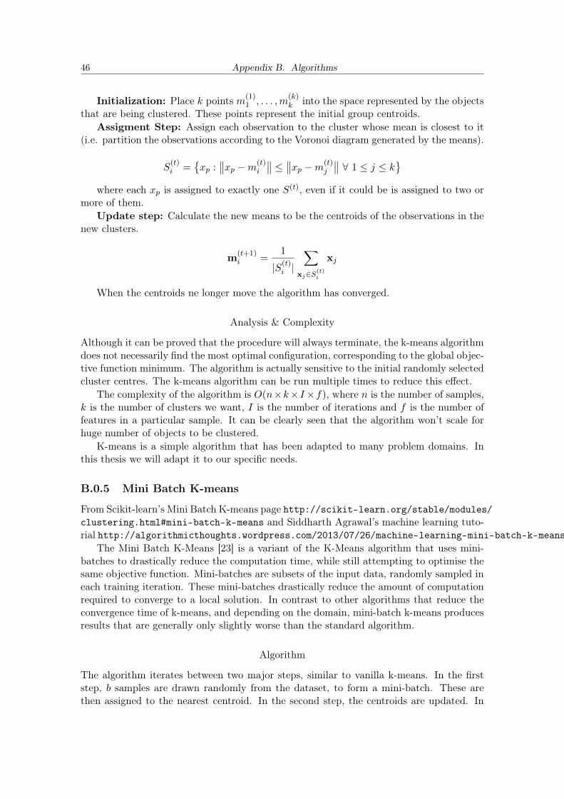
The algorithm iterates between two major steps, similar to vanilla k-means. In the firststep, b samples are drawn randomly from the dataset, to form a mini-batch. These arethen assigned to the nearest centroid. In the second step, the centroids are updated. In
47
contrast to k-means, this is done on a per-sample basis. For each sample in the mini-batch, the assigned centroid is updated by taking the streaming average of the sampleand all previous samples assigned to that centroid. This has the effect of decreasing therate of change for a centroid over time. These steps are performed until convergence or apredetermined number of iterations is reached.
Given: k, mini-batch size b, iterations t, data set XInitialize each c in C with an x picked randomly from Xv <- 0for i = 1 to t do
M <- b examples picked randomly from Xfor x in M do
d[x] <- f (C, x) // Cache the center nearest to xend forfor x in M do
c <- d[x] // Get cached center for this xv[c] <- v[c] + 1 // Update per-center countslr <- 1 / v[c] // Get per-center learning ratec <- (1 - lr)c + lr * x // Take gradient step
end forend for
Comparison with Kmeans
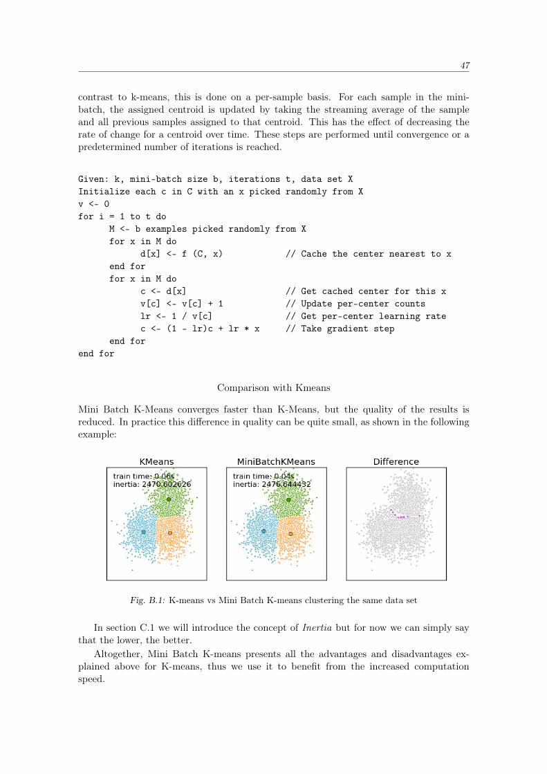
Mini Batch K-Means converges faster than K-Means, but the quality of the results isreduced. In practice this difference in quality can be quite small, as shown in the followingexample:
Fig. B.1: K-means vs Mini Batch K-means clustering the same data set
In section C.1 we will introduce the concept of Inertia but for now we can simply saythat the lower, the better.
Altogether, Mini Batch K-means presents all the advantages and disadvantages ex-plained above for K-means, thus we use it to benefit from the increased computationspeed.
48 Appendix B. Algorithms
B.0.6 DBSCAN
From DBSCAN’s Wikipedia article: http://en.wikipedia.org/wiki/DBSCAN.DBSCAN (Density-Based Spatial Clustering of Applications with Noise) is a clustering
algorithm proposed in 1996 by Martin Ester, Hans-Peter Kriegel, Jörg Sander et XiaoweiXu [5]. It is a density-based algorithm because it finds a number of clusters startingfrom the estimated density distribution of corresponding nodes. DBSCAN along with K-means are ones of the most common clustering algorithms and also most cited in scientificliterature.
Explanation
DBSCAN’s definition of a cluster is based on the notion of density reachability. Basically,a point q is directly density-reachable from a point p if it is not farther away than agiven distance ε (i.e., is part of its ε-neighborhood) and if p is surrounded by sufficientlymany points such that one may consider p and q to be part of a cluster. q is calleddensity-reachable (note the distinction from “directly density-reachable”) from p if there isa sequence p1, . . . , pn of points with p1 = p and pn = q where each pi is directly density-reachable from pi−1.
Note that the relation of density-reachable is not symmetric. q might lie on the edge ofa cluster, having insufficiently many neighbors to count as dense itself. This would halt theprocess of finding a path that stops with the first non-dense point. By contrast, startingthe process with q would lead to p (though the process would halt there, p being the firstnon-dense point). Due to this asymmetry, the notion of density-connected is introduced:two points p and q are density-connected if there is a point o such that both p and q aredensity-reachable from o. Density-connectedness is symmetric.
A cluster satisfies two properties:
• All points within the cluster are mutually density-connected.
• If a point is density-connected to any point of the cluster, it is part of the cluster aswell.
Algorithm
DBSCAN requires two parameters: ε (eps) and the minimum number of points requiredto form a cluster (minPts). It starts with an arbitrary starting point that has not beenvisited. This point’s ε-neighborhood is retrieved, and if it contains sufficiently many points,a cluster is started. Otherwise, the point is labeled as noise. Note that this point mightlater be found in a sufficiently sized ε-environment of a different point and hence be madepart of a cluster.
If a point is found to be a dense part of a cluster, its ε-neighborhood is also part ofthat cluster. Hence, all points that are found within the ε-neighborhood are added, asis their own ε-neighborhood when they are also dense. This process continues until thedensity-connected cluster is completely found. Then, a new unvisited point is retrievedand processed, leading to the discovery of a further cluster or noise.
49
Pseudocode
D is the set of the objects to be clustered, eps is ε and MinPts is the minimum numberof points required to form a cluster.
DBSCAN(D, eps, MinPts)C = 0for each unvisited point P in dataset D
mark P as visitedNeighborPts = regionQuery(P, eps)if sizeof(NeighborPts) < MinPts
mark P as NOISEelse
C = next clusterexpandCluster(P, NeighborPts, C, eps, MinPts)
expandCluster(P, NeighborPts, C, eps, MinPts)add P to cluster Cfor each point P’ in NeighborPts
if P’ is not visitedmark P’ as visitedNeighborPts’ = regionQuery(P’, eps)if sizeof(NeighborPts’) >= MinPts
NeighborPts = NeighborPts joined with NeighborPts’if P’ is not yet member of any cluster
add P’ to cluster C
regionQuery(P, eps)return all points within P’s eps-neighborhood (including P)
Complexity
DBSCAN visits each point of the dataset, possibly multiple times (e.g., as candidates todifferent clusters). For practical considerations, however, the time complexity is mostlygoverned by the number of regionQuery invocations. DBSCAN executes exactly one suchquery for each point, and if an indexing structure is used that executes such a neighborhoodquery in O
(log n
), an overall runtime complexity of O
(n · log n
)is obtained. Without the
use of an accelerating index structure, the run time complexity isO(n2). Often the distance
matrix of size (n2 − n)/2 is materialized to avoid distance recomputations. This howeveralso needs O
(n2)memory.
Advantages
• It does not require one to specify the number of clusters in the data a priori, asopposed to k-means.
• It can find arbitrarily shaped clusters. It can even find a cluster completely sur-rounded by (but not connected to) a different cluster. Due to the MinPts parame-ter, the so-called single-link effect (different clusters being connected by a thin lineof points) is reduced.
50 Appendix B. Algorithms
• It has a notion of noise.
• It requires just two parameters and is mostly insensitive to the ordering of the points.(However, points sitting on the edge of two different clusters might swap clustermembership if the ordering of the points is changed, and the cluster assignment isunique only up to isomorphism.)
• It is designed for use with structures that can accelerate region queries, e.g. usingan R∗ tree.
Disadvantages
• The quality of DBSCAN depends on the metric used in the function regionQuery(P, ε).The most common distance metric used is the Euclidean distance. Especially forhigh-dimensional data, this metric can be rendered almost useless due to the so-called “Curse of dimensionality”, making it difficult to find an appropriate value forε. This effect, however, is also present in any other algorithm based on the Euclideandistance.
• It cannot cluster data sets well with large differences in densities, since theminPts−εcombination cannot then be chosen appropriately for all clusters.
B.0.7 QuickBundles
From Garydallidis et al. paper “QuickBundles, a method for tractography simplification”[7].
QuickBundles (QB) is a simple and very fast algorithm which can reduce tractographyrepresentation to an accessible structure in a time that is linear in the number of tracts N .
In QB each item (tract) is a fixed-length ordered sequence of points in R3, and QB usescomparison functions and amalgamations that take account of and preserve this structure.Moreover each item is either added to an existing cluster on the basis of the distancesbetween the cluster descriptor of the item and the descriptors of the current list of clusters.Clusters are held in a list which is extended according to need. Unlike amalgamationclustering algorithms such as K-means [12, 27] or BIRCH [34], there is no reassignment orupdating phase in QB – once an item is assigned to a cluster it stays there, and clustersare not amalgamated. QB derives its speed from this idea.
QB uses the minimum average direct flip distance (MDF) described before (tracts areresampled to k points each). QB stores information about clusters in cluster nodes. Tractsare indexed with i = 1 . . . N where si is the K × 3 matrix representing tract i. A clusternode is defined as a triple c = (I, h, n) where I is the list of the integer indices i = 1 . . . Nof the tracts in that cluster, n is the number of tracts in the cluster, and h is the tractsum. h is a K × 3 matrix which can be updated on the fly when a tract is added to acluster and is equal to:
h =n∑i=1
si
where si is the K × 3 matrix representing i-th tract, and n is the number of tracts inthe cluster. The centroid tract is calculated as v = h/n.
51
Algorithm
The algorithm proceeds as follows. At any one step in the algorithm there are M clusters.Select the first tract s1 and place it in the first cluster c1 ← (1, s1, 1). M = 1 at this point.For each remaining tract in turn i = 3 . . . N :
1. calculate the MDF distance between tract si and the centroid tracts ve of all thecurrent clusters ce, e = 1 . . .M , where v is defined on the fly as v = h/n
2. if any of the MDF values me are smaller than a clustering threshold θ add tract ito the cluster e with the minimum value for me; ce = (I, h, n), and update ce ←(append(I, i), h+ s, n+ 1)
3. otherwise create a new cluster cM+1 ← ([i], si, 1),M ←M + 1.
Choice of orientation can become an issue when adding tracts together, because tractscan equivalently have their points ordered 1 . . . k or be flipped with order k . . . 1. A stepin QB takes account of the possibility of needing to perform such a flip of a tract beforeadding it to a centroid tract according to which direction produced the lowest MDF value.
Complexity
The complexity of QB is in the best case linear time O(N)with the number of tracts N
and worst case O(N2)when every cluster contains only one tracts. The average case is
O(MN
)where M is the number of clusters. One of the reasons why QB has on average
linear time complexity derives from the structure of the cluster node: they only savethe sum of current tracts h in the cluster and the sum is cumulative; moreover there isno recalculation of clusters, the streamlines are passed through only once and a tract isassigned to one cluster only.

52 Appendix B. Algorithms
Appendix C
SCORES
C.1 Inertia
Some sections are from Scikit-learn’s section on Inertia http://scikit-learn.org/stable/modules/clustering.html#inertia
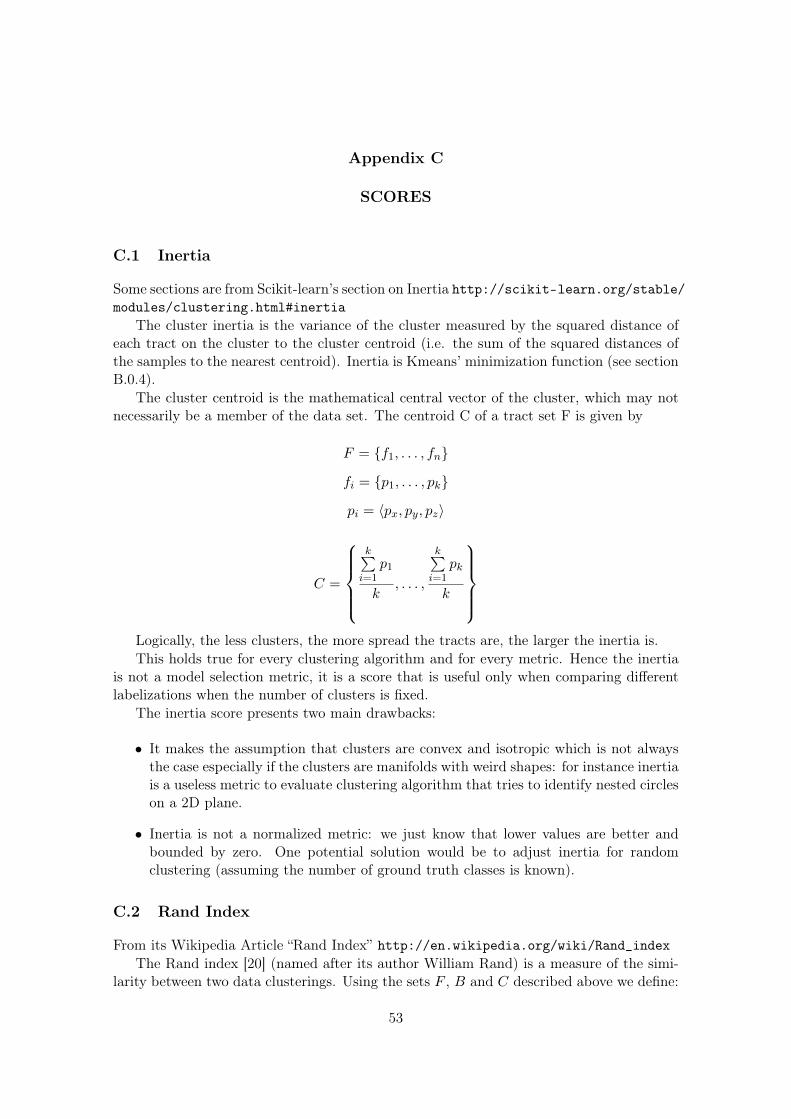
The cluster inertia is the variance of the cluster measured by the squared distance ofeach tract on the cluster to the cluster centroid (i.e. the sum of the squared distances ofthe samples to the nearest centroid). Inertia is Kmeans’ minimization function (see sectionB.0.4).
The cluster centroid is the mathematical central vector of the cluster, which may notnecessarily be a member of the data set. The centroid C of a tract set F is given by
F = {f1, . . . , fn}
fi = {p1, . . . , pk}
pi = 〈px, py, pz〉
C =
k∑i=1
p1
k, . . . ,
k∑i=1
pk
k
Logically, the less clusters, the more spread the tracts are, the larger the inertia is.This holds true for every clustering algorithm and for every metric. Hence the inertia
is not a model selection metric, it is a score that is useful only when comparing differentlabelizations when the number of clusters is fixed.
The inertia score presents two main drawbacks:
• It makes the assumption that clusters are convex and isotropic which is not alwaysthe case especially if the clusters are manifolds with weird shapes: for instance inertiais a useless metric to evaluate clustering algorithm that tries to identify nested circleson a 2D plane.
• Inertia is not a normalized metric: we just know that lower values are better andbounded by zero. One potential solution would be to adjust inertia for randomclustering (assuming the number of ground truth classes is known).
C.2 Rand Index
From its Wikipedia Article “Rand Index” http://en.wikipedia.org/wiki/Rand_indexThe Rand index [20] (named after its author William Rand) is a measure of the simi-
larity between two data clusterings. Using the sets F , B and C described above we define:
53
54 Appendix C. Scores
• a = |{(fi, fj)/fi, fj ∈ Bk, fi, fj ∈ Cl}|the number of pairs of elements in F that are in the same set in B and in the sameset in C
• b = |{(fi, fj)/fi ∈ Bk1 , fj ∈ Bk2 , fi ∈ Cl1 , fj ∈ Cl2}|the number of pairs of elements in F that are in different sets in B and in differentsets in C
• c = |{(fi, fj)/fi, fj ∈ Bk, fi ∈ Cl1 , fj ∈ Cl2}|the number of pairs of elements in F that are in the same set in B and in differentsets in C
• d = |{(fi, fj)|fi ∈ Bk1 , fj ∈ Bk2 , fi, fj ∈ Cl}|the number of pairs of elements in F that are in different sets in B and in the sameset in C
for some 1 ≤ i, j ≤ n, i 6= j, 1 ≤ k, k1, k2 ≤ r, k1 6= k2, 1 ≤ l, l1, l2 ≤ s, l1 6= l2.The Rand Index is thus defined as:
RI =a+ b
a+ b+ c+ d=a+ b
(n2 )
Intuitively, a+ b can be considered as the number of agreements between B and C andc+ d as the number of disagreements between B and C.
The Rand index has a value between 0 and 1, with 0 indicating that the two dataclusters do not agree on any pair of points and 1 indicating that the data clusters areexactly the same.
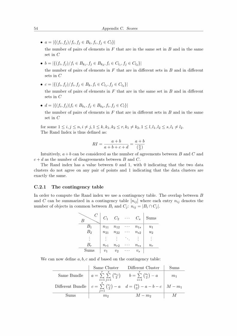
C.2.1 The contingency table
In order to compute the Rand index we use a contingency table. The overlap between Band C can be summarized in a contingency table [nij ] where each entry nij denotes thenumber of objects in common between Bi and Cj : nij = |Bi ∩ Cj |.
HHHHHHBC
C1 C2 · · · Cs Sums
B1 n11 n12 · · · n1s u1B2 n21 n22 · · · ns2 u2...
......
. . ....
...Br nr1 nr2 · · · nrs ur
Sums v1 v2 · · · vs
We can now define a, b, c and d based on the contingency table:
Same Cluster Different Cluster Sums
Same Bundle a =r∑i=1
s∑j=1
(nij2
)b =
r∑i=1
(ui2
)− a m1
Different Bundle c =s∑j=1
(vj2
)− a d =
(n2
)− a− b− c M −m1
Sums m2 M −m2 M
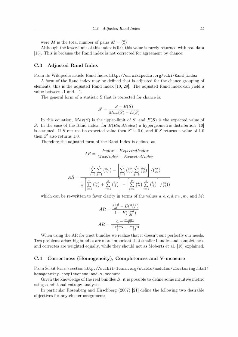
C.3. Adjusted Rand Index 55
were M is the total number of pairs M =(n2
)Although the lower-limit of this index is 0.0, this value is rarely returned with real data
[15]. This is because the Rand index is not corrected for agreement by chance.
C.3 Adjusted Rand Index
From its Wikipedia article Rand Index http://en.wikipedia.org/wiki/Rand_index.A form of the Rand index may be defined that is adjusted for the chance grouping of
elements, this is the adjusted Rand index [10, 29]. The adjusted Rand index can yield avalue between -1 and +1.
The general form of a statistic S that is corrected for chance is:
S′ =S − E(S)
Max(S)− E(S)
In this equation, Max(S) is the upper-limit of S, and E(S) is the expected value ofS. In the case of the Rand index, for E(RandIndex) a hypergeometric distribution [10]is assumed. If S returns its expected value then S′ is 0.0, and if S returns a value of 1.0then S′ also returns 1.0.
Therefore the adjusted form of the Rand Index is defined as
AR =Index− ExpectedIndex
MaxIndex− ExpectedIndex
AR =
r∑i=1
s∑j=1
(nij2
)−
[r∑i=1
(ai2
) s∑j=1
(bj2
)]/(n2
))
12
[r∑i=1
(ai2
)+
s∑j=1
(bj2
)]−
[r∑i=1
(ai2
) s∑j=1
(bj2
)]/(n2
))
which can be re-written to favor clarity in terms of the values a, b, c, d,m1,m2 and M :
AR =a+dM − E(a+dM )
1− E(a+dM )
AR =a− m1m2
Mm1+m2
2 − m1m2M
When using the AR for tract bundles we realize that it doesn’t suit perfectly our needs.Two problems arise: big bundles are more important that smaller bundles and completenessand correctes are weighted equally, while they should not as Moberts et al. [16] explained.
C.4 Correctness (Homogeneity), Completeness and V-measure
From Scikit-learn’s section http://scikit-learn.org/stable/modules/clustering.html#homogeneity-completeness-and-v-measure
Given the knowledge of the real bundles B, it is possible to define some intuitive metricusing conditional entropy analysis.
In particular Rosenberg and Hirschberg (2007) [21] define the following two desirableobjectives for any cluster assignment:
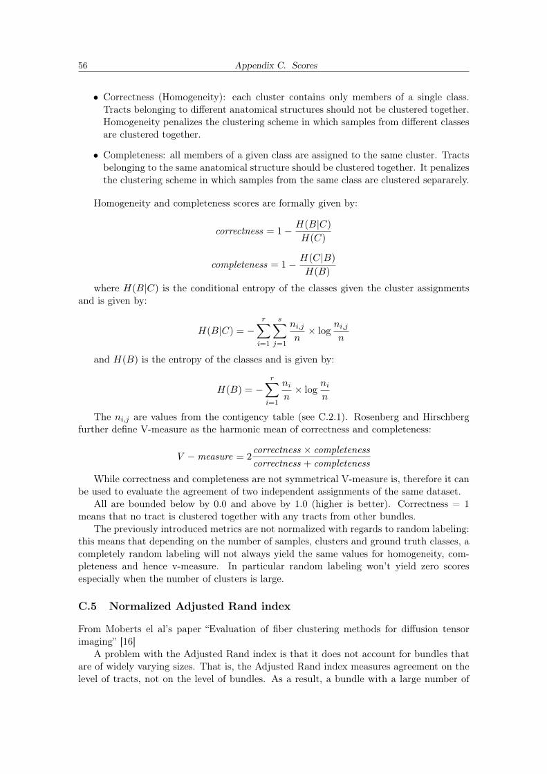
56 Appendix C. Scores
• Correctness (Homogeneity): each cluster contains only members of a single class.Tracts belonging to different anatomical structures should not be clustered together.Homogeneity penalizes the clustering scheme in which samples from different classesare clustered together.
• Completeness: all members of a given class are assigned to the same cluster. Tractsbelonging to the same anatomical structure should be clustered together. It penalizesthe clustering scheme in which samples from the same class are clustered separarely.
Homogeneity and completeness scores are formally given by:
correctness = 1− H(B|C)
H(C)
completeness = 1− H(C|B)
H(B)
where H(B|C) is the conditional entropy of the classes given the cluster assignmentsand is given by:
H(B|C) = −r∑i=1
s∑j=1
ni,jn× log
ni,jn
and H(B) is the entropy of the classes and is given by:
H(B) = −r∑i=1
nin× log
nin
The ni,j are values from the contigency table (see C.2.1). Rosenberg and Hirschbergfurther define V-measure as the harmonic mean of correctness and completeness:
V −measure = 2correctness × completeness
correctness + completeness
While correctness and completeness are not symmetrical V-measure is, therefore it canbe used to evaluate the agreement of two independent assignments of the same dataset.
All are bounded below by 0.0 and above by 1.0 (higher is better). Correctness = 1means that no tract is clustered together with any tracts from other bundles.
The previously introduced metrics are not normalized with regards to random labeling:this means that depending on the number of samples, clusters and ground truth classes, acompletely random labeling will not always yield the same values for homogeneity, com-pleteness and hence v-measure. In particular random labeling won’t yield zero scoresespecially when the number of clusters is large.
C.5 Normalized Adjusted Rand index
From Moberts el al’s paper “Evaluation of fiber clustering methods for diffusion tensorimaging” [16]
A problem with the Adjusted Rand index is that it does not account for bundles thatare of widely varying sizes. That is, the Adjusted Rand index measures agreement on thelevel of tracts, not on the level of bundles. As a result, a bundle with a large number of
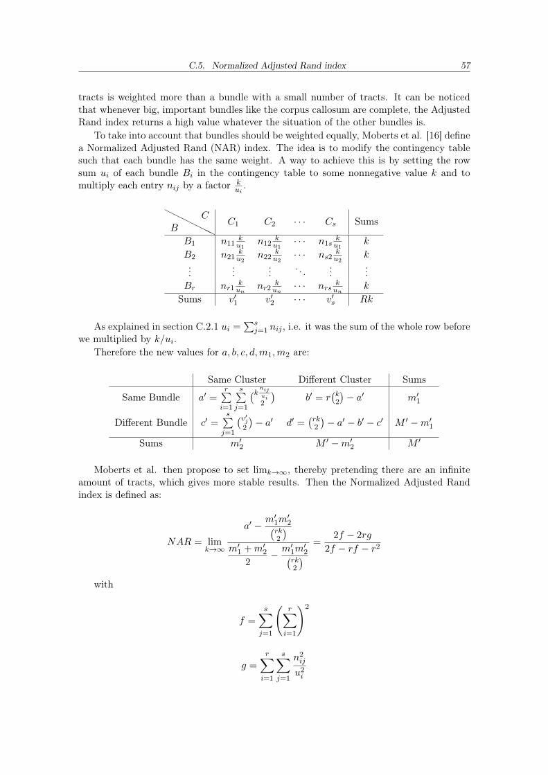
C.5. Normalized Adjusted Rand index 57
tracts is weighted more than a bundle with a small number of tracts. It can be noticedthat whenever big, important bundles like the corpus callosum are complete, the AdjustedRand index returns a high value whatever the situation of the other bundles is.
To take into account that bundles should be weighted equally, Moberts et al. [16] definea Normalized Adjusted Rand (NAR) index. The idea is to modify the contingency tablesuch that each bundle has the same weight. A way to achieve this is by setting the rowsum ui of each bundle Bi in the contingency table to some nonnegative value k and tomultiply each entry nij by a factor k
ui.
HHHHHHBC
C1 C2 · · · Cs Sums
B1 n11ku1
n12ku1
· · · n1sku1
k
B2 n21ku2
n22ku2
· · · ns2ku2
k...
......
. . ....
...Br nr1
kun
nr2kun
· · · nrskun
k
Sums v′1 v′2 · · · v′s Rk
As explained in section C.2.1 ui =∑s
j=1 nij , i.e. it was the sum of the whole row beforewe multiplied by k/ui.
Therefore the new values for a, b, c, d,m1,m2 are:
Same Cluster Different Cluster Sums
Same Bundle a′ =r∑i=1
s∑j=1
(k nijui2
)b′ = r
(k2
)− a′ m′1
Different Bundle c′ =s∑j=1
(v′j2
)− a′ d′ =
(rk2
)− a′ − b′ − c′ M ′ −m′1
Sums m′2 M ′ −m′2 M ′
Moberts et al. then propose to set limk→∞, thereby pretending there are an infiniteamount of tracts, which gives more stable results. Then the Normalized Adjusted Randindex is defined as:
NAR = limk→∞
a′ − m′1m′2(
rk2
)m′1 +m′2
2− m′1m
′2(
rk2
) =2f − 2rg
2f − rf − r2
with
f =
s∑j=1
(r∑i=1
)2
g =
r∑i=1
s∑j=1
n2iju2i
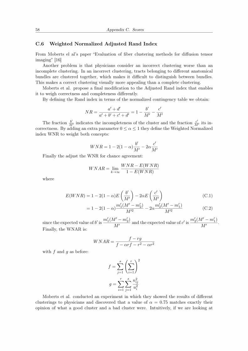
58 Appendix C. Scores
C.6 Weighted Normalized Adjusted Rand Index
From Moberts el al’s paper “Evaluation of fiber clustering methods for diffusion tensorimaging” [16]
Another problem is that physicians consider an incorrect clustering worse than anincomplete clustering. In an incorrect clustering, tracts belonging to different anatomicalbundles are clustered together, which makes it difficult to distinguish between bundles.This makes a correct clustering visually more appealing than a complete clustering.
Moberts et al. propose a final modification to the Adjusted Rand index that enablesit to weigh correctness and completeness differently.
By defining the Rand index in terms of the normalized contingency table we obtain:
NR =a′ + d′
a′ + b′ + c′ + d′= 1− b′
M ′− c′
M ′
The fraction b′
M ′ indicates the incompleteness of the cluster and the fraction c′
M ′ its in-correctness. By adding an extra parameter 0 ≤ α ≤ 1 they define the Weighted Normalizedindex WNR to weight both concepts:
WNR = 1− 2(1− α)b′
M ′− 2α
c′
M ′
Finally the adjust the WNR for chance agreement:
WNAR = limk→∞
WNR− E(WNR)
1− E(WNR)
where
E(WNR) = 1− 2(1− α)E
(b′
M ′
)− 2αE
(c′
M ′
)(C.1)
= 1− 2(1− α)m′1(M
′ −m′2)M ′2
− 2αm′2(M
′ −m′1)M ′2
(C.2)
since the expected value of b′ ism′1(M
′ −m′2)M ′
and the expected value of c′ ism′2(M
′ −m′1)M ′
.Finally, the WNAR is:
WNAR =f − rg
f − αrf − r2 − αr2
with f and g as before:
f =
s∑j=1
(r∑i=1
)2
g =
r∑i=1
s∑j=1
n2iju2i
Moberts et al. conducted an experiment in which they showed the results of differentclusterings to physicians and discovered that a value of α = 0.75 matches exactly theiropinion of what a good cluster and a bad cluster were. Intuitively, if we are looking at
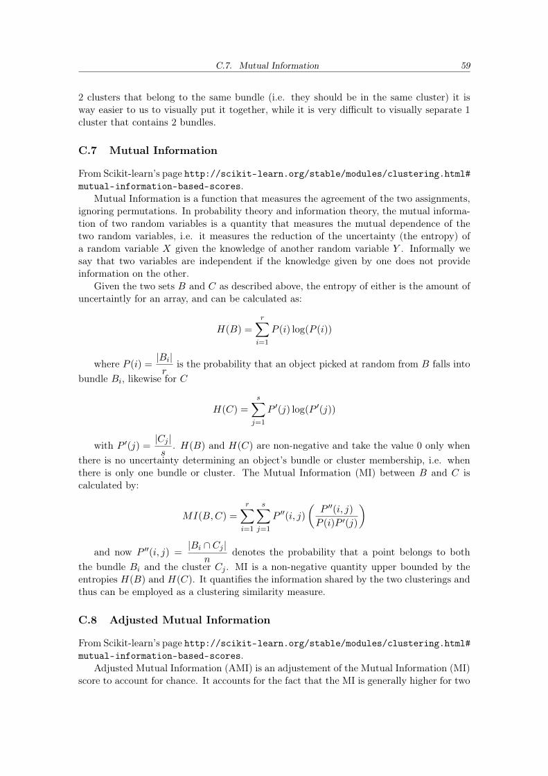
C.7. Mutual Information 59
2 clusters that belong to the same bundle (i.e. they should be in the same cluster) it isway easier to us to visually put it together, while it is very difficult to visually separate 1cluster that contains 2 bundles.
C.7 Mutual Information
From Scikit-learn’s page http://scikit-learn.org/stable/modules/clustering.html#mutual-information-based-scores.
Mutual Information is a function that measures the agreement of the two assignments,ignoring permutations. In probability theory and information theory, the mutual informa-tion of two random variables is a quantity that measures the mutual dependence of thetwo random variables, i.e. it measures the reduction of the uncertainty (the entropy) ofa random variable X given the knowledge of another random variable Y . Informally wesay that two variables are independent if the knowledge given by one does not provideinformation on the other.
Given the two sets B and C as described above, the entropy of either is the amount ofuncertaintly for an array, and can be calculated as:
H(B) =r∑i=1
P (i) log(P (i))
where P (i) =|Bi|r
is the probability that an object picked at random from B falls intobundle Bi, likewise for C
H(C) =
s∑j=1
P ′(j) log(P ′(j))
with P ′(j) =|Cj |s
. H(B) and H(C) are non-negative and take the value 0 only whenthere is no uncertainty determining an object’s bundle or cluster membership, i.e. whenthere is only one bundle or cluster. The Mutual Information (MI) between B and C iscalculated by:
MI(B,C) =r∑i=1
s∑j=1
P ′′(i, j)
(P ′′(i, j)
P (i)P ′(j)
)
and now P ′′(i, j) =|Bi ∩ Cj |
ndenotes the probability that a point belongs to both
the bundle Bi and the cluster Cj . MI is a non-negative quantity upper bounded by theentropies H(B) and H(C). It quantifies the information shared by the two clusterings andthus can be employed as a clustering similarity measure.
C.8 Adjusted Mutual Information
From Scikit-learn’s page http://scikit-learn.org/stable/modules/clustering.html#mutual-information-based-scores.
Adjusted Mutual Information (AMI) is an adjustement of the Mutual Information (MI)score to account for chance. It accounts for the fact that the MI is generally higher for two
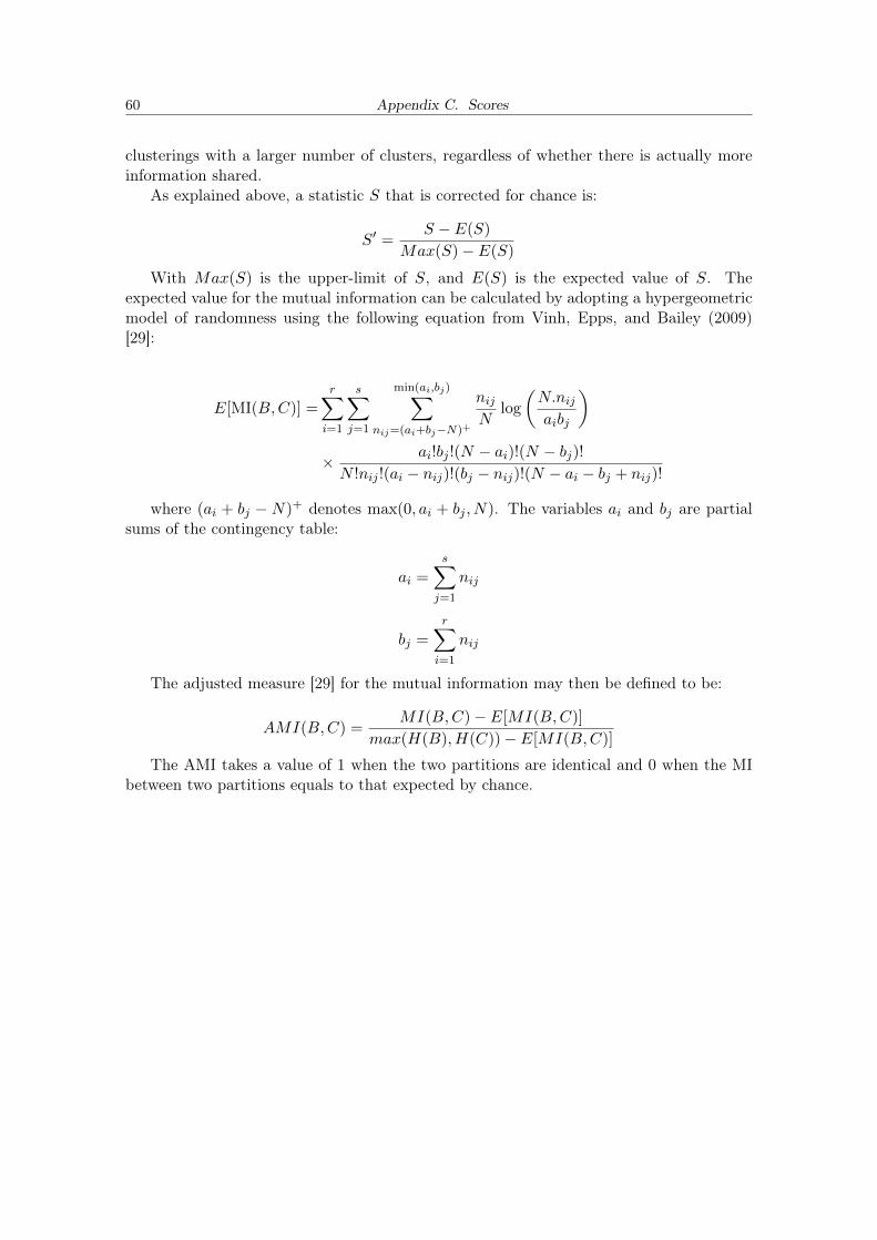
60 Appendix C. Scores
clusterings with a larger number of clusters, regardless of whether there is actually moreinformation shared.
As explained above, a statistic S that is corrected for chance is:
S′ =S − E(S)
Max(S)− E(S)
With Max(S) is the upper-limit of S, and E(S) is the expected value of S. Theexpected value for the mutual information can be calculated by adopting a hypergeometricmodel of randomness using the following equation from Vinh, Epps, and Bailey (2009)[29]:
E[MI(B,C)] =r∑i=1
s∑j=1
min(ai,bj)∑nij=(ai+bj−N)+
nijN
log
(N.nijaibj
)
× ai!bj !(N − ai)!(N − bj)!N !nij !(ai − nij)!(bj − nij)!(N − ai − bj + nij)!
where (ai + bj − N)+ denotes max(0, ai + bj , N). The variables ai and bj are partialsums of the contingency table:
ai =
s∑j=1
nij
bj =
r∑i=1
nij
The adjusted measure [29] for the mutual information may then be defined to be:
AMI(B,C) =MI(B,C)− E[MI(B,C)]
max(H(B), H(C))− E[MI(B,C)]
The AMI takes a value of 1 when the two partitions are identical and 0 when the MIbetween two partitions equals to that expected by chance.

BIBLIOGRAPHY
[1] Guillaume Auzias et al. Disco: A coherent diffeomorphic framework for brain regis-tration under exhaustive sulcal constraints. In LNCS, volume 5761, pages 730–738,2009.
[2] Matthan W A Caan, Lucas J van Vliet, Charles B L M Majoie, Maaike M van derGraaff, C. A. Grimbergen, and Frans M Vos. Nonrigid point set matching of whitematter tracts for diffusion tensor image analysis. IEEE Trans Biomed Eng, 58(9):2431–2440, Sep 2011.
[3] Lynn E. DeLisi et al. Early detection of schizophrenia by diffusion weighted imaging.Psychiatry Research: Neuroimaging, 148(1):61 – 66, 2006.
[4] Stanley Durrleman, Pierre Fillard, Xavier Pennec, Alain Trouvé, and Nicholas Ayache.A statistical model of white matter fiber bundles based on currents. Inf Process MedImaging, 21:114–125, 2009.
[5] Martin Ester, Hans peter Kriegel, Jörg S, and Xiaowei Xu. A density-based algorithmfor discovering clusters in large spatial databases with noise. pages 226–231. AAAIPress, 1996.
[6] C. Fowlkes, S. Belongie, Fan Chung, and J. Malik. Spectral grouping using the nys-trom method. Pattern Analysis and Machine Intelligence, IEEE Transactions on,26(2):214–225, 2004.
[7] Eleftherios Garyfallidis et al. Quickbundles, a method for tractography simplification.Frontiers in Neuroscience, 6(175), 2012.
[8] P. Guevara, D. Duclap, C. Poupon, L. Marrakchi-Kacem, P. Fillard, D. Le Bihan,M. Leboyer, J. Houenou, and J-F. Mangin. Automatic fiber bundle segmentationin massive tractography datasets using a multi-subject bundle atlas. Neuroimage,61(4):1083–1099, Jul 2012.
[9] P. Guevara, C. Poupon, D. Rivière, Y. Cointepas, M. Descoteaux, B. Thirion, and J-F.Mangin. Robust clustering of massive tractography datasets. Neuroimage, 54(3):1975–1993, Feb 2011.
[10] Lawrence Hubert and Phipps Arabie. Comparing partitions. Journal of Classification,2(1):193–218, December 1985.
[11] Hai Li, Zhong Xue, Lei Guo, Tianming Liu, Jill Hunter, and Stephen T CWong. A hy-brid approach to automatic clustering of white matter fibers. Neuroimage, 49(2):1249–1258, Jan 2010.
[12] J. MacQueen. Some methods for classification and analysis of multivariate observa-tions. In Proc. Fifth Berkeley Symp. on Math. Statist. and Prob., volume 1, pages281–297. Univ. of Calif. Press, 1967.
61
62 Bibliography
[13] Mahnaz Maddah, W. Eric L Grimson, Simon K Warfield, and William M Wells. Aunified framework for clustering and quantitative analysis of white matter fiber tracts.Med Image Anal, 12(2):191–202, Apr 2008.
[14] Mahnaz Maddah, James V Miller, Edith V Sullivan, Adolf Pfefferbaum, and TorstenRohlfing. Sheet-like white matter fiber tracts: representation, clustering, and quanti-tative analysis. Med Image Comput Comput Assist Interv, 14(Pt 2):191–199, 2011.
[15] Glenn W. Milligan and Martha C. Cooper. A study of the comparability of externalcriteria for hierarchical cluster analysis. Multivariate Behavioral Research, 21(4):441–458, 1986.
[16] B. Moberts, A. Vilanova, and J.J. van Wijk. Evaluation of fiber clustering methodsfor diffusion tensor imaging. In Visualization, 2005. VIS 05. IEEE, pages 65 – 72,oct. 2005.
[17] Andriy Myronenko, Xubo Song, and Miguel Carreira-Perpinan. Non-rigid point setregistration: Coherent point drift. In B. Schölkopf, J. Platt, and T. Hoffman, editors,Advances in Neural Information Processing Systems (NIPS) 19, pages 1009–1016. MITPress, Cambridge, MA, 2007.
[18] L. J. O’Donnell, M. Kubicki, M. E. Shenton, M. H. Dreusicke, W. E L Grimson,and C. F. Westin. A method for clustering white matter fiber tracts. AJNR Am JNeuroradiol, 27(5):1032–1036, May 2006.
[19] F. Pedregosa et al. Scikit-learn: Machine learning in Python. Journal of MachineLearning Research, 12:2825–2830, 2011.
[20] William M. Rand. Objective criteria for the evaluation of clustering methods. Journalof the American Statistical Association, 66(336):846–850, 1971.
[21] Andrew Rosenberg and Julia Hirschberg. V-Measure: A Conditional Entropy-BasedExternal Cluster Evaluation Measure. In Proceedings of the 2007 Joint Conferenceon Empirical Methods in Natural Language Processing and Computational NaturalLanguage Learning (EMNLP-CoNLL), pages 410–420, 2007.
[22] Peter J. Rousseeuw. Silhouettes: A graphical aid to the interpretation and validationof cluster analysis. JCAM, 20(0):53 – 65, 1987.
[23] D. Sculley. Web-scale k-means clustering. In Proceedings of the 19th internationalconference on World wide web, WWW ’10, pages 1177–1178, New York, NY, USA,2010. ACM.
[24] V. Siless, S. Medina, G. Varoquaux, and B. Thirion. A comparison of metrics andalgorithms for fiber clustering. In Pattern Recognition in Neuroimaging (PRNI), 2013International Workshop on, pages 190–193, 2013.
[25] Viviana Siless et al. Joint T1 and brain fiber log-demons registration using currentsto model geometry. In MICCAI, pages 57–65, 2012.
Bibliography 63
[26] Viviana Siless, Pamela Guevara, Xavier Pennec, and Pierre Fillard. Joint T1 and BrainFiber Diffeomorphic Registration Using the Demons. In Tianming Liu, DinggangShen, Luis Ibanez, and Xiaodong Tao, editors, Multimodal Brain Image Analysis,volume 7012 of Lecture Notes in Computer Science, pages 10–18. Springer Berlin /Heidelberg, 2011.
[27] H. Steinhaus. Sur la division des corp materiels en parties. Bull. Acad. Polon. Sci,1:801–804, 1956.
[28] N. Toussaint, J.C. Souplet, and P. Fillard. Medinria: Medical image navigation andresearch tool by inria. In Proc. of MICCAI’07 Workshop on Interaction in medicalimage analysis and visualization, Brisbane, Australia, 2007.
[29] Nguyen Xuan Vinh, Julien Epps, and James Bailey. Information theoretic measuresfor clusterings comparison: is a correction for chance necessary? In Proceedings ofthe 26th Annual International Conference on Machine Learning, ICML ’09, pages1073–1080, New York, NY, USA, 2009. ACM.
[30] Qian Wang, Pew-Thian Yap, Guorong Wu, and Dinggang Shen. Application of neu-roanatomical features to tractography clustering. Hum Brain Mapp, Mar 2012.
[31] Xiaogang Wang, W. Eric L Grimson, and Carl-Fredrik Westin. Tractography segmen-tation using a hierarchical dirichlet processes mixture model. Neuroimage, 54(1):290–302, Jan 2011.
[32] D. Wassermann, L. Bloy, E. Kanterakis, R. Verma, and R. Deriche. Unsupervisedwhite matter fiber clustering and tract probability map generation: applications of agaussian process framework for white matter fibers. Neuroimage, 51(1):228–241, May2010.
[33] Yan Xia, U. Turken, Susan L Whitfield-Gabrieli, and John D Gabrieli. Knowledge-based classification of neuronal fibers in entire brain. Med Image Comput ComputAssist Interv, 8(Pt 1):205–212, 2005.
[34] Tian Zhang, Raghu Ramakrishnan, and Miron Livny. Birch: An efficient data clus-tering method for very large databases, 1996.
[35] Orly Zvitia, Arnaldo Mayer, Ran Shadmi, Shmuel Miron, and Hayit K Greenspan.Co-registration of white matter tractographies by adaptive-mean-shift and gaussianmixture modeling. IEEE Trans Med Imaging, 29(1):132–145, Jan 2010.