University of Birmingham Research Archive

e-theses repository This unpublished thesis/dissertation is copyright of the author and/or third parties. The intellectual property rights of the author or third parties in respect of this work are as defined by The Copyright Designs and Patents Act 1988 or as modified by any successor legislation. Any use made of information contained in this thesis/dissertation must be in accordance with that legislation and must be properly acknowledged. Further distribution or reproduction in any format is prohibited without the permission of the copyright holder.

ABSTRACT

Intermediate level nuclear waste (ILW) will be stored above ground in 304L stainless

steel (SS) containers for the next 100 years. During this period, the containers need to

be monitored for atmospheric pitting corrosion - a known precursor of atmospherically

induced stress corrosion cracking. Hyperspectral (HS) and optical imaging of pitting

corrosion products from droplet experiments have been investigated towards

developing a system for long term monitoring of atmospheric pitting corrosion of

stainless steel containers in ILW stores.

Common corrosion products were first identified via Raman spectroscopic mapping as

akaganeite (β-FeOOH) and lepidocrocite (γ-FeOOH), with a secondary presence of

layered double hydroxide (green rust).

HS and optical methods were then compared for their efficacy at rust detection. Whilst

it was not possible to identify specific corrosion species using HS imaging, HS images

of rust under pitted droplets provided better contrast with the background steel than

colour photography due to species having lower absorbance the near infrared (850 nm)

than red (650 nm).

Finally, the relationship between rust area and pit volume was determined by

comparing colour photography (rust area) with confocal laser scanning microscopy (pit

volume). A good correlation was present for samples exposed to a fixed relative

humidity (RH) for MgCl2 droplets and CaCl2 droplets with small pit volumes. Poor

correlation was found for samples exposed to natural fluctuations in RH. It was

concluded that optical methods are viable for the detection of rust, but less effective for

quantification of pit volumes.

Dedicated to my family and friends

Two roads diverged in a yellow wood, And sorry I could not travel both And be one traveler, long I stood

And looked down one as far as I could To where it bent in the undergrowth;

Then took the other, as just as fair,

And having perhaps the better claim, Because it was grassy and wanted wear;

Though as for that the passing there Had worn them really about the same,

And both that morning equally lay

In leaves no step had trodden black. Oh I kept the first for another day!

Yet knowing how way leads on to way, I doubted if I should ever come back.

I shall be telling this with a sigh

Somewhere ages and ages hence: Two roads diverged in a wood, and I-

I took the one less traveled by, And that has made all the difference

-‘The Road not Taken’, Robert Frost[1]

ACKNOWLEDGEMENTS

I owe thanks to the advice and support of a great many people, without whom

this project would not have been possible:

First and foremost my supervisors Professor Alison Davenport, whose

guidance, support and patience have been limitless during the course of this

project.

Secondly, my supervisor Professor Hamid Dehghani, his insight and experience

have been invaluable for the imaging sections of this project.

I would also like to thank the Nuclear Decommissioning Authority for making

this project possible and my industrial supervisor David Hambley from NNL for

much productive discussion and the perspective of industry.

To my friends and colleagues Steven, Angus, Sarah, Haval, Flaviu, Rowena,

Sophie, Qi and Berenika in Metallurgy and Materials and Sophie in Computer

Science who I’ve had the fortune to call on for many hours of productive

discussion

Last but not least I’d like to thank my friends and family for their unwavering

support and encouragement over these past few years.

i

Table of Contents 1. INTRODUCTION .......................................................................................... 1

2. LITERATURE REVIEW ................................................................................ 3

2.1 Interim storage of intermediate level nuclear waste ............................... 3

2.1.1 Overview ......................................................................................... 3

2.1.2 Conditions within waste stores ........................................................ 4

2.1.3 Temperature and humidity .............................................................. 4

2.1.4 Aerosol deposition ........................................................................... 5

2.2 Stainless Steel ....................................................................................... 6

2.3 Corrosion ............................................................................................... 7

2.3.1 Overview ......................................................................................... 7

2.3.2 Passivity .......................................................................................... 8

2.3.3 Pitting corrosion of stainless steel ................................................... 8

2.3.4 Atmospheric pitting corrosion ........................................................ 11

2.3.5 Atmospherically induced stress corrosion cracking ....................... 16

2.4 Corrosion products of iron .................................................................... 17

2.4.1 Formation and transformation of the iron oxides ........................... 18

2.4.2 Characterisation of iron oxides and oxide-hydroxides ................... 20

2.4.3 Atmospheric corrosion products of iron alloys ............................... 21

2.4.4 Corrosion products of stainless steel ............................................. 22

2.5 Corrosion detection and monitoring ..................................................... 23

2.5.1 Principles of imaging and spectroscopy ....................................... 24

ii

2.5.2 Hyperspectral imaging ................................................................... 26

2.5.3 Image analysis .............................................................................. 28

2.6 Summary ............................................................................................. 32

3. Methodology ............................................................................................... 33

3.1 Droplet experiments ............................................................................. 33

3.1.1 Materials and sample preparation ................................................. 33

3.1.2 Solution preparation ...................................................................... 34

3.1.3 Droplet deposition ......................................................................... 35

3.1.4 Exposure to fixed environmental conditions .................................. 36

3.1.5 Exposure to fluctuating ambient environmental conditions ............ 37

3.2 Photography ........................................................................................ 38

3.3 Iron oxide syntheses ............................................................................ 39

3.4 Characterisation and Spectroscopy ..................................................... 40

3.4.1 X-ray diffraction ............................................................................. 40

3.4.2 UV-VIS-NIR spectroscopy ............................................................. 40

3.4.3 Fourier-Transform Infra-Red (FTIR) spectroscopy ........................ 41

3.4.4 Raman Spectroscopy .................................................................... 42

3.5 UV-VIS-NIR Hyperspectral Imaging ..................................................... 44

3.5.1 Hyperspectral instrument hardware, motion control and data

acquisition .................................................................................................. 44

3.5.2 Characterisation of UV-VIS hyperspectral imaging system ........... 47

iii

3.6 Rust area analysis ............................................................................... 57

3.6.1 Red-Blue colour channel subtraction ............................................. 58

3.6.2 Principal component analysis ........................................................ 58

3.6.3 HSV thresholding .......................................................................... 58

3.6.4 L*a*b* thresholding ........................................................................ 59

3.7 Confocal microscopy for pit volume measurement .............................. 60

4. CHARACTERISATION OF CORROSION PRODUCTS OF 304L STAINLESS STEEL USING COLOUR PHOTOGRAPHY AND RAMAN SPECTROSCOPY ............................................................................................ 61

4.1 Introduction .......................................................................................... 61

4.2 Results ................................................................................................. 63

4.2.1 Synthesised Iron Oxides and oxide-hydroxides ............................ 63

4.2.2 Droplet Experiments ...................................................................... 70

4.2.3 Exposure conditions for fluctuating ambient droplets .................... 89

4.3 Discussion ........................................................................................... 93

4.3.1 Identification and assignment of compounds ................................ 93

4.3.2 Distribution of compounds by cation .............................................. 95

4.3.3 Distribution of compounds over time ............................................. 96

4.3.4 Distribution of compounds by chloride deposition density ............. 96

4.4 Conclusions ......................................................................................... 97

5. EVALUATION OF HYPERSPECTRAL METHODS .................................... 99

5.1 Introduction .......................................................................................... 99

5.2 Results ............................................................................................... 100

iv

5.2.1 UV-VIS-NIR for iron oxide phase identification ............................ 100

5.2.2 Comparison of techniques for area quantification ....................... 116

5.3 Discussion ......................................................................................... 122

5.3.1 Iron oxide phase identification using UV-VIS-NIR imaging .......... 122

5.3.2 Techniques for area quantification/Image analysis...................... 126

5.4 Conclusions ....................................................................................... 129

6. ASSESSMENT OF PIT VOLUME WITH RESPECT TO VISIBLE RUST AREA .............................................................................................................. 131

6.1 Introduction ........................................................................................ 131

6.2 Results ............................................................................................... 133

6.2.1 Measurement of Pit Volume via confocal laser scanning

microscopy ............................................................................................... 135

6.2.2 Estimating error in pit volume due to user controlled parameters 143

6.2.3 Determination of threshold for Red-Blue colour channel subtraction

method …………………………………………………………………………145

6.2.4 Determination of threshold for principal component analysis method

………………………………………………………………………....147

6.2.5 Determination of threshold for HSV thresholding method ........... 149

6.2.6 Determination of threshold for L*a*b* thresholding method ......... 151

6.2.7 Rust area vs. pit volume .............................................................. 155

6.2.8 Ambient exposure conditions ...................................................... 163

6.3 Discussion ......................................................................................... 164

v

6.3.1 Pit volume measurements ........................................................... 164

6.3.2 Rust area measurement .............................................................. 165

6.3.3 Pit volume rust area comparison ................................................. 167

6.4 Conclusions ....................................................................................... 169

7. GENERAL DISCUSSION ......................................................................... 171

7.1 Limitations .......................................................................................... 173

8. GENERAL CONCLUSIONS ..................................................................... 174

9. FUTURE WORK ....................................................................................... 176

10. REFERENCES ......................................................................................... 178

11. APPENDIX ............................................................................................... 187

11.1 Mill certificate – 304L stainless steel .............................................. 187

11.2 Powdered iron oxide standard synthesis ........................................ 188

11.3 Matlab script – Raman averaging ................................................... 191

11.3.1 Main file - Spectral averaging ................................................... 191

11.3.2 Dependency – import csv spectral from directory .................... 193

11.4 Matlab scripts – Hyperspectral image processing .......................... 194

11.4.1 Principal component analysis ................................................... 194

11.5 Matlab scripts – Image processing ................................................. 195

11.5.1 Acquire rust area by Red-Blue colour channel subtraction ...... 195

11.5.2 Acquire rust area by principal component analysis .................. 197

11.5.3 Acquire rust area by HSV thresholding .................................... 199

11.5.4 Rust area analysis by L*a*b* thresholding ............................... 200

11.5.5 Supplemental figures (Chapter 6) ............................................ 203

vi

vii

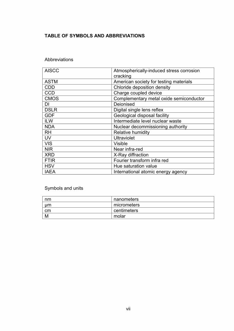
TABLE OF SYMBOLS AND ABBREVIATIONS

Abbreviations

AISCC Atmospherically-induced stress corrosion cracking

ASTM American society for testing materials

CDD Chloride deposition density

CCD Charge coupled device

CMOS Complementary metal oxide semiconductor

DI Deionised

DSLR Digital single lens reflex

GDF Geological disposal facility

ILW Intermediate level nuclear waste

NDA Nuclear decommissioning authority

RH Relative humidity

UV Ultraviolet

VIS Visible

NIR Near infra-red

XRD X-Ray diffraction

FTIR Fourier transform infra red

HSV Hue saturation value

IAEA International atomic energy agency

Symbols and units

nm nanometers

μm micrometers

cm centimeters

M molar

1

1. INTRODUCTION

The UK’s Nuclear Decommissioning Authority (NDA) estimates that it will have

to dispose of 286,000m3 of intermediate level nuclear waste.[2] This includes

legacy waste from previous nuclear projects as well as a projection of waste

produced from future commitments. The current long term disposal plan

favoured by both the UK NDA and the International Atomic Energy Agency

(IAEA) is internment in a geological disposal in facility (GDF) deep

underground. This will require many years to plan and implement.

As no deep GDF yet exists, waste will remain above ground, stored in

warehouses for a significant interim period while a site is selected and

prepared. During this period the containers housing the waste may be

susceptible to atmospheric corrosion. The containers are constructed of

stainless steel which displays good resistance to general corrosion, but it is

susceptible to localised corrosion known as pitting. Pitting corrosion does not

significantly affect the structural integrity of the container, but has been

identified as a precursor to atmospherically-induced stress corrosion cracking

(AISCC) which might lead to loss of structural integrity when containers are

moved to the GDF. It is therefore desirable to monitor the development of pitting

corrosion as a precursor to AISCC. As established corrosion detection

techniques rely on quantifying material loss, pitting is difficult to detect.

Corrosion pitting attack leads to formation of a rust scale on the surface of the

container, meaning optical detection methods are of interest.

2

Hyperspectral imaging is a well-established technique used to detect and

quantify similar iron rich compounds in other fields [3-5], Hyperspectral imaging

therefore presents a possible avenue for the remote sensing of the corrosion

product that forms around pitting on stainless steel.

This project aims to investigate the applicability of hyperspectral imaging and

conventional “RGB” colour imaging to monitor atmospheric pitting corrosion in

stores. The overall aim of the project is to identify likely corrosion products,

determine the optimum imaging method for quantifying visible rust, and then to

use this method to determine the relationship between corrosion pit volume and

visible rust.

3

2. LITERATURE REVIEW

2.1 Interim storage of intermediate level nuclear waste

2.1.1 Overview

Nuclear waste is separated into levels based on hazard and heat output as a

measure of impact on repository design; the types are low, intermediate and

high level waste. Intermediate level waste is radioactive, but does not produce

heat in large enough quantities to require additional, specialist cooling. [2, 6]

The UK government’s policy for long term disposal of this waste is in a large

underground repository called a geological disposal facility (GDF). There will be

an interim period of up to 100 years while the site of the GDF is selected, the

facility is prepared and the waste is moved. During this time, the waste is to be

immobilised in concrete and stored above ground in containers made of 316L

and 304L stainless steel[2, 7]

During this period in above-ground storage, the containers will be susceptible to

atmospheric pitting corrosion from gradual deposition and deliquescence of

chloride salts from the atmosphere. While pitting is the expected mode of

corrosion and not likely to affect the structural integrity of the container in itself,

it is a known precursor of atmospherically-induced stress corrosion cracking

(AISCC) which could compromise container integrity and complicate waste

transfer to the GDF.[8]

4

2.1.2 Conditions within waste stores

The risk of occurrence of atmospheric corrosion is dependent on the local

atmospheric conditions. The NDA has commissioned surveys to determine the

environment that the waste containers will be exposed to until they are moved

to the geological disposal facility.

2.1.3 Temperature and humidity

There are several current ILW stores located around the UK. Encapsulated

product stores (EPS) 1 and 2, located at Sellafield are currently subject to

environmental control aimed at reducing surface wetting of the containers from

condensation, others are passively ventilated[9]. The conditions of stores under

passive ventilation will be subject to local weather conditions although the

shelter provided by the buildings will slow any rapid variations.

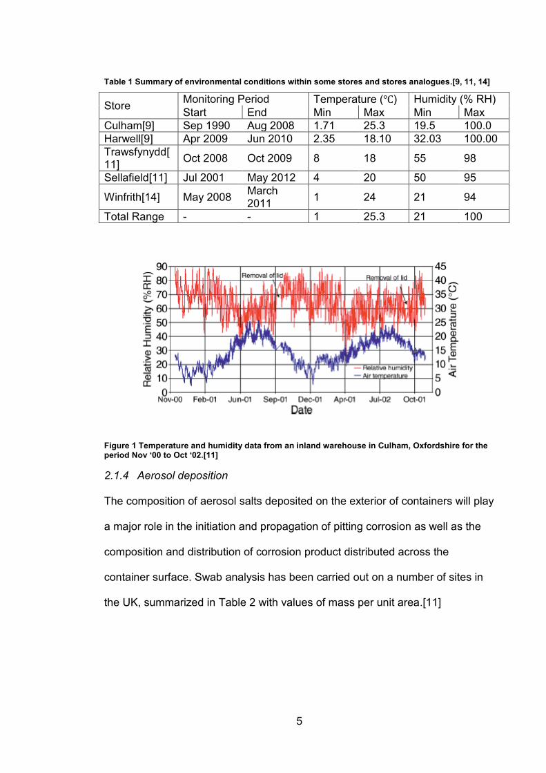
While present in interim storage the surface temperature of the containers

expected to follow the trend of the local environment.[10] Temperature and

humidity maximum and minimum values for a number of stores fluctuated

between near-freezing and high room temperature (Table 1), with more precise

time resolved data from Culham (Figure 1) indicating that conditions follow the

seasons with higher humidity and lower temperature present in winter

months.[9, 11-13]

5

Table 1 Summary of environmental conditions within some stores and stores analogues.[9, 11, 14]

Store Monitoring Period Temperature (℃) Humidity (% RH)

Start End Min Max Min Max

Culham[9] Sep 1990 Aug 2008 1.71 25.3 19.5 100.0

Harwell[9] Apr 2009 Jun 2010 2.35 18.10 32.03 100.00

Trawsfynydd[11]

Oct 2008 Oct 2009 8 18 55 98

Sellafield[11] Jul 2001 May 2012 4 20 50 95

Winfrith[14] May 2008 March 2011

1 24 21 94

Total Range - - 1 25.3 21 100

Figure 1 Temperature and humidity data from an inland warehouse in Culham, Oxfordshire for the period Nov ‘00 to Oct ‘02.[11]

2.1.4 Aerosol deposition

The composition of aerosol salts deposited on the exterior of containers will play

a major role in the initiation and propagation of pitting corrosion as well as the

composition and distribution of corrosion product distributed across the

container surface. Swab analysis has been carried out on a number of sites in

the UK, summarized in Table 2 with values of mass per unit area.[11]

6

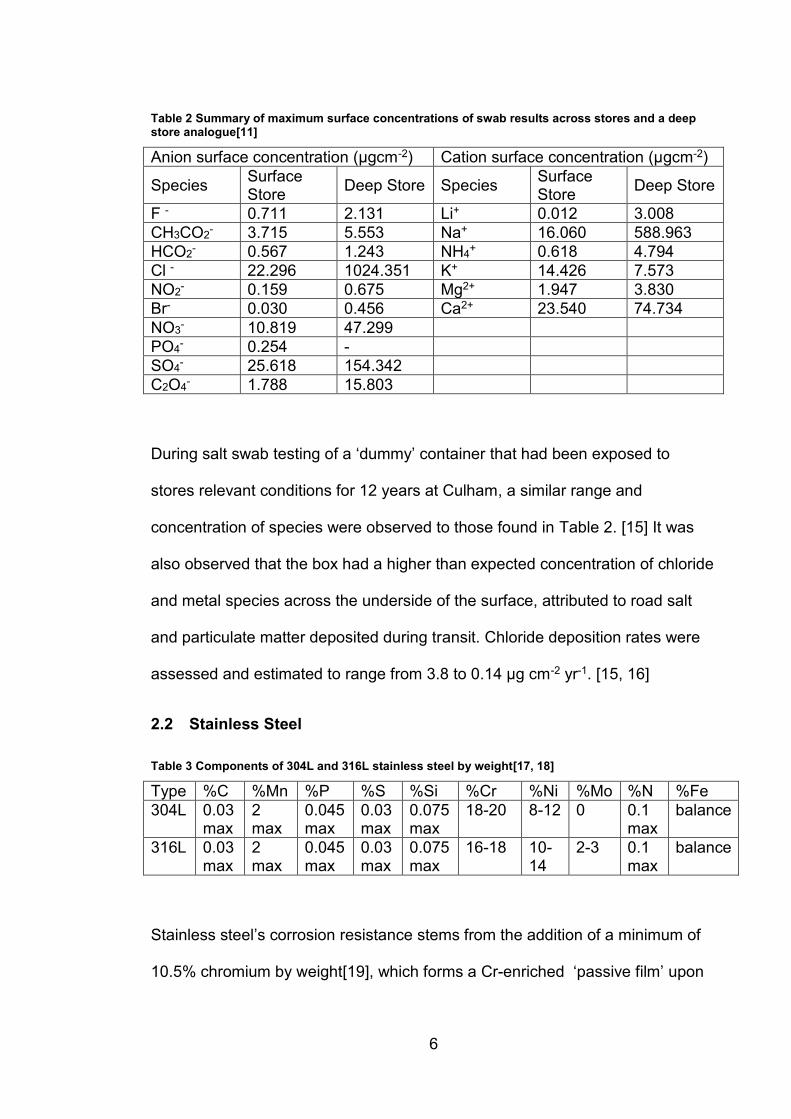
Table 2 Summary of maximum surface concentrations of swab results across stores and a deep store analogue[11]

Anion surface concentration (μgcm-2) Cation surface concentration (μgcm-2)

Species Surface Store

Deep Store Species Surface Store

Deep Store

F - 0.711 2.131 Li+ 0.012 3.008

CH3CO2- 3.715 5.553 Na+ 16.060 588.963

HCO2- 0.567 1.243 NH4

+ 0.618 4.794

Cl - 22.296 1024.351 K+ 14.426 7.573

NO2- 0.159 0.675 Mg2+ 1.947 3.830

Br- 0.030 0.456 Ca2+ 23.540 74.734

NO3- 10.819 47.299

PO4- 0.254 -

SO4- 25.618 154.342

C2O4- 1.788 15.803

During salt swab testing of a ‘dummy’ container that had been exposed to

stores relevant conditions for 12 years at Culham, a similar range and

concentration of species were observed to those found in Table 2. [15] It was

also observed that the box had a higher than expected concentration of chloride

and metal species across the underside of the surface, attributed to road salt

and particulate matter deposited during transit. Chloride deposition rates were

assessed and estimated to range from 3.8 to 0.14 μg cm-2 yr-1. [15, 16]

2.2 Stainless Steel

Table 3 Components of 304L and 316L stainless steel by weight[17, 18]

Type %C %Mn %P %S %Si %Cr %Ni %Mo %N %Fe

304L 0.03 max

2 max

0.045 max

0.03 max

0.075 max

18-20 8-12 0 0.1 max

balance

316L 0.03 max

2 max

0.045 max

0.03 max

0.075 max

16-18 10-14

2-3 0.1 max

balance

Stainless steel’s corrosion resistance stems from the addition of a minimum of

10.5% chromium by weight[19], which forms a Cr-enriched ‘passive film’ upon

7

contact with the air[20]. This acts to protect the bulk metal from corrosive

environments, increasing the resistance to uniform corrosion.[19] 304L and

316L are common austenitic stainless steel grades have a higher %wt of

chromium, as outlined in Table 3. 316L is differentiated from 304L by the

addition of 2-4%wt molybdenum which further enhances the resistance to

localised corrosion.[21]

304L and 316L stainless steel are both austenitic stainless steels, however

some residual ferrite is known to persist throughout the manufacturing

process.[22]

2.3 Corrosion

2.3.1 Overview

Corrosion is an electrochemical process involving the oxidation and dissolution

of a metal, which occurs at an anode. For iron, the anodic (oxidation) reaction

is:

Fe ⇌ Fe2+ + 2e- Equation 1

For oxidation to take place, it is necessary for the electrons to be consumed in a

cathodic (reduction) reaction. The typical cathodic reaction is reduction of

oxygen:

2H2O + O2 +4e- ⇌ 4OH- Equation 2

When iron corrodes, the soluble ferrous ions may react with the hydroxide ions

produced in the cathodic reaction and oxygen from the air to form rust, which is

typically an iron oxy-hydroxide with the general formula FeOOH:

8

4Fe2+ + O2 + 8OH- ⇌ 4FeOOH + 2H2O Equation 3

Equation 3 is one example of charge being balanced by combining the metal

and hydroxide ions, forming an iron hydroxide which will precipitate out of the

solution as corrosion product. The equilibrium point of the reaction in equation 1

and therefore whether a metal is likely to undergo dissolution is governed by the

reduction potential and pH of the system. A potential-pH or ‘Pourbaix’ diagram

can be used to indicate graphically whether or not corrosion might be

thermodynamically favourable in certain conditions.[23]

2.3.2 Passivity

Passivity occurs when environmental conditions thermodynamically favour the

growth of an insoluble metal-oxide layer several atoms thick which prevents the

metal underneath from contact with the environment.[24]. On stainless steels

this film is enriched in Cr2O3 which is stable under a wide range of conditions

and strongly adheres to the underlying metal. The addition of a significant %wt

of chromium as an alloying element also gives stainless steel the ability to ‘heal’

this Cr-rich passive film as selective dissolution of Fe will cause the surface

layer to rapidly once again become enriched with Cr.[20, 25]

2.3.3 Pitting corrosion of stainless steel

Pitting corrosion of stainless steel usually initiates at MnS or oxide inclusions.

Anodic dissolution of the metal forms metal ions which react with water

(hydrolysis) forming H+ ions which lower the local pH, e.g. Equation 4 for iron.

This decreases pH and prevents the passive oxide layer from reforming within

the pit.[26]

9

Fe2+ + H2O ⇌ Fe(OH)+ + H+ Equation 4

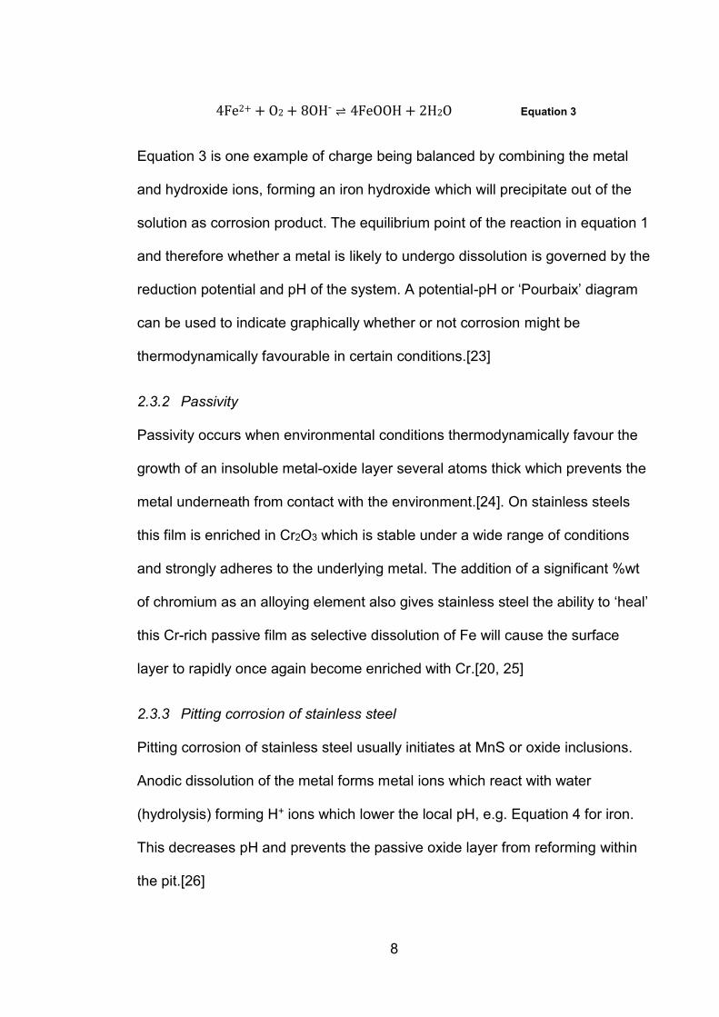
Pitting corrosion of stainless steel is a well-studied phenomenon in full

immersion conditions and proceeds in three stages; initiation, meta-stable

pitting and propagation.[8, 27].

Figure 2 Representation of passive film breakdown via the point defect model[28]

Initiation first requires the breakdown of the protective passive Cr2O3 film

(Figure 2). This almost always occurs at the site of a metallographic inclusion in

stainless steels, usually manganese sulphide in the case of austenitic stainless

steels[8, 29-32], but pitting has also been reported to initiate at other inclusions

such as multi-element oxides[30, 33-35]. Inclusions which are not

thermodynamically stable are then likely to wholly or partially dissolve and leave

a cavity or occluded site which can prevent aggressive chemistry from being

10

diluted by the bulk solution.[29, 31, 36, 37] As a result, the metal continues to

dissolve and the pit continues to grow.

While this occluded geometry persists, the pit will go through a period of rapid

growth, eventually the passive film above will rupture and the pit solution mixes

with the bulk electrolyte. Many pits repassivate at this point as the pH and metal

ion concentration inside the pit is no longer low enough to sustain active

dissolution. If a young pit repassivates in this manner it’s said to have been

meta-stable. If the rate of diffusion of metal ions out of the pit is equal to or

exceeded by the rate of those leaving the metal surface however, the

aggressive conditions will be maintained, dissolution will continue and the pit

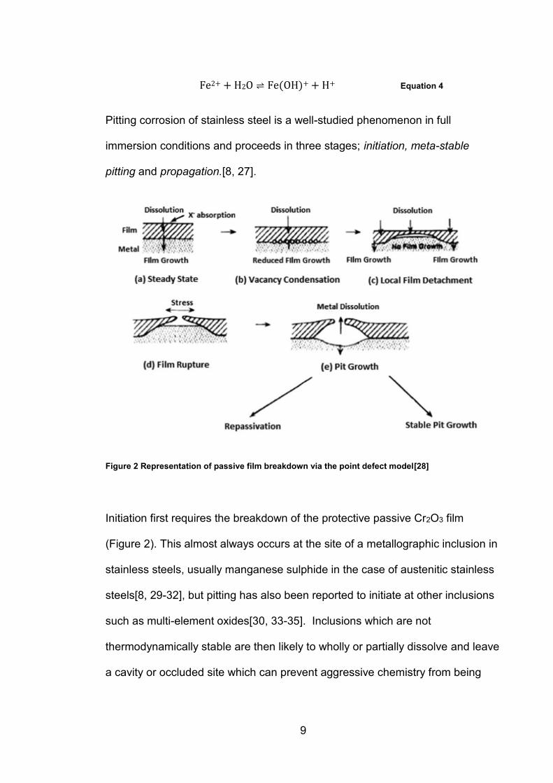
will continue to propagate[26, 38].

Figure 3 Representation of the key processes involved during propagation of pitting of metal in NaCl solution in non-occluded conditions[39]

11

The large number of positively charged species in the pit draws anions from the

bulk solution to maintain charge balance, Cl- being of particular note as it

remains fully dissociated from H+ ions, allowing a large concentration of them to

remain in the pit and maintain a low pH.

As a result of this occluded geometry and ion exchange with the bulk solution, a

concentration gradient of metal ions occurs between the pit mouth and the site

of active dissolution, which can super-saturate and cause a layer of salt to

form.[40-42] This can act as a reservoir of metal ions and protect the pit against

sudden, temporary changes in conditions which could otherwise cause the

active surface to repassivate.[43, 44]

2.3.4 Atmospheric pitting corrosion

Atmospheric pitting occurs with deposition of aerosol salts that absorb water

from the atmosphere or ‘deliquesce’ to form a thin, confined layer of solution or

‘droplet’. At equilibrium, the water activity is equal to that of the relative humidity

the surrounding atmospheric environment. There are several interconnected

factors which can affect the severity of this attack: relative humidity of the

environment, the density of chloride deposited on the metal surface and the

microstructure of the metal.

The relative humidity of the environment controls the solution concentration as

any deposited salt will absorb or expel water until it reaches equilibrium with the

water activity of the air. As a result, relative humidity (together with the chloride

deposition density) governs the total volume of electrolyte as well as the

resistivity and diffusivity of the solution. All salt species differ in the minimum

12

relative humidity at which they absorb enough water from the air (deliquesce) to

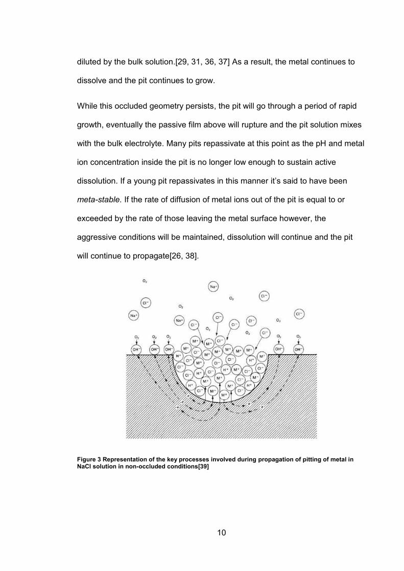
form a saturated solution. For example, MgCl2 has a deliquescence humidity of

33% RH at 30°C and so will form a saturated solution above this relative

humidity. This will become less concentrated if humidity increases, as shown in

Figure 4a.[45]

Due to the confined nature of the solution, a ‘three phase boundary’ exists

between the metal, the solution and the air. This was first explored by Evans in

his seminal work where it was observed that the cathodic reactions are most

likely to happen towards the droplet edge due to high O2 availability via diffusion

from the surrounding air[46]. The size of the droplet can therefore also affect the

corrosion process. A wider droplet area is associated with a larger pit mouth

diameter[47] and a higher probability of pitting[45, 48]. Droplet thickness is

controlled by a combination of the relative humidity and the salt deposition

density (CDD) on the metal surface. An increase in local RH will reduce the

solution concentration and therefore increase the diffusivity and conductivity of

the droplet (to a point, see Figure 4b), while a higher CDD will give a thicker

droplet for a particular RH and therefore increase the overall conductance of the

droplet and distance that O2 needs to travel to reach a cathodic region from the

droplet surface. Consequently, both RH and CDD have a significant effect on

the growth rate of pits.[47, 49]

13

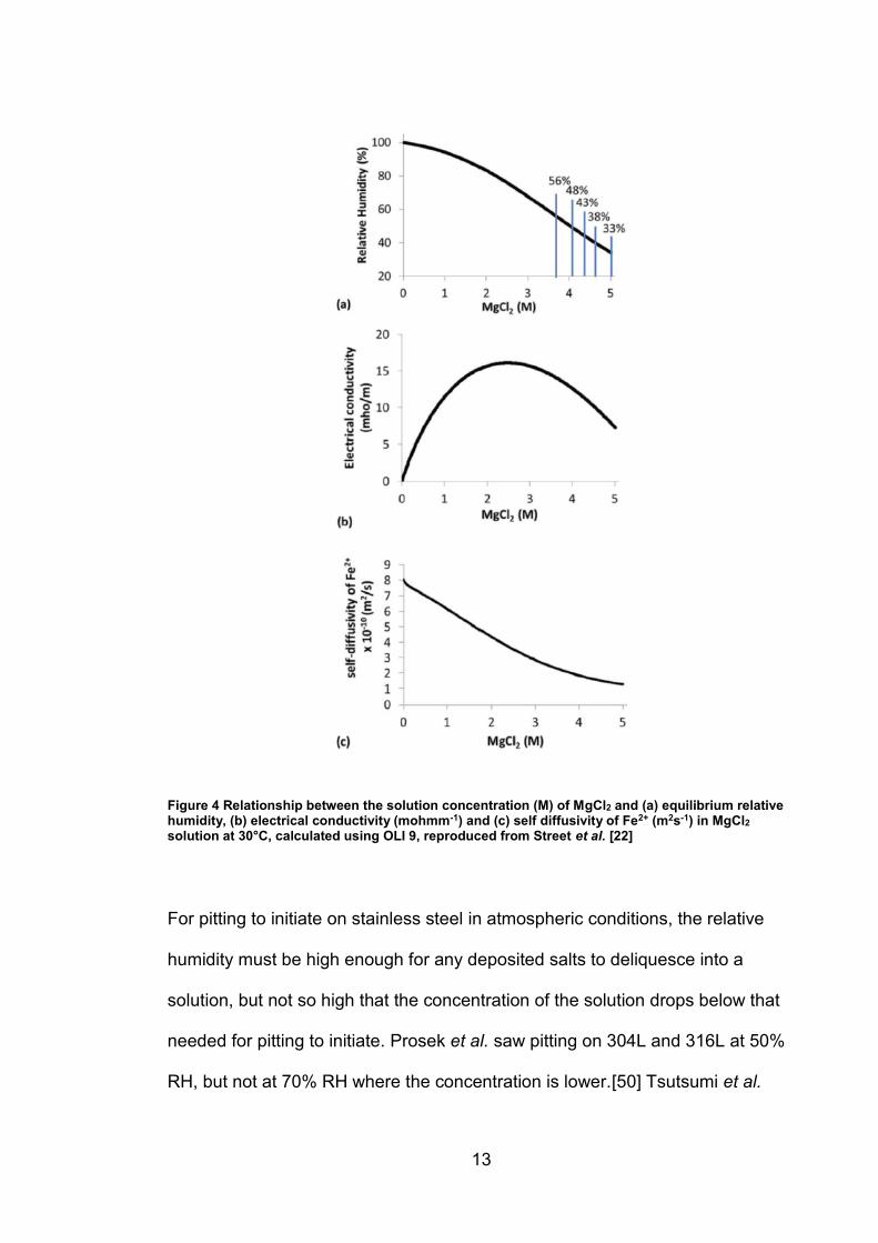
Figure 4 Relationship between the solution concentration (M) of MgCl2 and (a) equilibrium relative humidity, (b) electrical conductivity (mohmm-1) and (c) self diffusivity of Fe2+ (m2s-1) in MgCl2 solution at 30°C, calculated using OLI 9, reproduced from Street et al. [22]

For pitting to initiate on stainless steel in atmospheric conditions, the relative

humidity must be high enough for any deposited salts to deliquesce into a

solution, but not so high that the concentration of the solution drops below that

needed for pitting to initiate. Prosek et al. saw pitting on 304L and 316L at 50%

RH, but not at 70% RH where the concentration is lower.[50] Tsutsumi et al.

14

also investigated pitting on 304 stainless steel under MgCl2 droplets and saw

pitting between 65% and 75% RH. [45, 51, 52]

As the relative humidity of the environment rarely stays constant, work has been

done to characterise the effects of fluctuating conditions on the pitting process

in situations where the electrolyte repeatedly dries out, or ‘wet-dry’ cycling

conditions. It is widely accepted that pits will repassivate during the ‘wetting’

stage (high RH) while during the ‘drying’ stage, new pits will initiated and

grow.[44, 52-56] Nam et al. isolated initiation and repassivation events under

MgCl2 droplets using electrochemical methods. They observed initiation at 47-

58% RH for 304 and 48-58% RH for 430 at 298k, and noted repassivation at

56-70% RH for 304 and 67-73% for 430.[57] During wet and dry cycles a

droplet’s viscosity and conductance vary, which will significantly affect the rate

of corrosion. Wet-dry cycling is likely to be more aggressive overall than

constant exposure to a thin electrolyte due to multiple initiation events.[58-60]

2.3.4.1 Morphology of pitting

The shape of pits can have a significant effect on how the pit propagates and

vary depending on the metallographic structure and on the exposure conditions.

In full immersion conditions pits are often hemispherical and require some form

of additional occlusion to maintain an aggressive environment. This can be

provided by a ‘lacy cover’ as has been observed over in the initial stages of

growth of these pits.[61]

In atmospheric conditions, pits have been shown to grow with different

morphologies to full immersion conditions. ‘Shallow dish’ regions[52, 62, 63] are

15

prominent on young pits which can either develop into ‘spirals’ or ‘satellites’

depending on conditions.[63, 64] It has also been shown that preferential

dissolution and therefore pit propagation can occur along bands of residual δ-

ferrite in the metal sub-surface.[65]

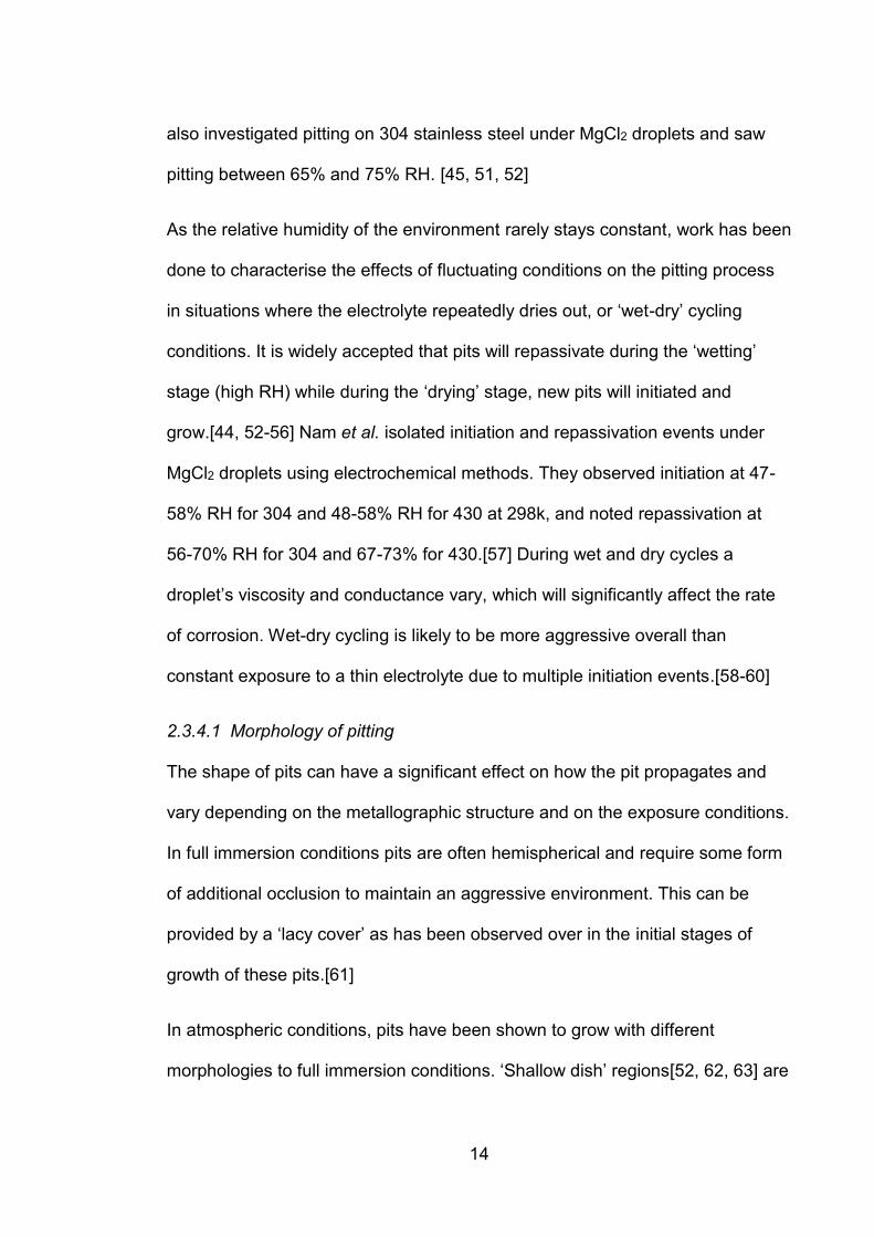
RH has also been found to significantly influence pit morphology, with Street et

al. observing ‘satellite' morphology at lower RH values (33%) and ‘spiral’

morphologies at 43-48%RH, along with a shallow dish region. At 56% RH, no

shallow dishes were present instead a deeper, rougher morphology was

observed[22] This was attributed to differences in solution diffusivity and

conductivity producing a higher IR drop for droplets exposed to lower RH

conditions. Street also reported that the diameter of the shallow dish region

varies with distance from the droplet edge, with smaller diameters seen at

locations closer to the droplet edge.

Figure 5 Typical examples of pit morphologies grown under MgCl2 droplets with CDD of 750 μgcm-2 after exposure at constant RH for 1 day at 30°C. (a) and (b) show satellite morphologies, (b-e) spiral pits, (f) circular pit [22]

16

2.3.5 Atmospherically induced stress corrosion cracking

Pitting itself does not significantly affect the structural integrity of the attacked

metal, but it is a known precursor of atmospherically induced stress corrosion

cracking (AISCC) in high chloride environments. The major contributing factors

to risk of AISCC risk that are relevant to this project are temperature (higher

temperatures increase risk), solution composition (higher chloride

concentrations increase risk) and tensile stress (higher stresses increase risk)

with cracks developing perpendicular to the applied stress.[39] It is generally

accepted that austenitic stainless steels are resistant to AISCC as long as the

temperature remains below ~50°C, this is due to the fact that stress corrosion

cracking can only develop from an active pit if the rate of pit growth is lower

than that of the rate of crack growth[66, 67]. There have been high profile

exceptions to this, however, where chloride induced AISCC failures of austenitic

stainless steels have occurred in swimming pools and coastal areas.[68-70]

Austenitic stainless steels such as the 304L and 316L used to fabricate

Intermediate level waste containers will be susceptible around the welds used

to affix the lids and laser etched identifiers due to residual stress and depletion

of chromium increasing susceptibility to corrosion respectively.[71, 72] Stress

corrosion cracking can compromise the structural integrity of the container and

so identifying sites at risk of AISCC via detecting the development of the pitting

precursor is the primary motivation of this project.

17

2.4 Corrosion products of iron

Rust is the collective name for the mix of iron(II/III) oxide species which form the

corrosion product when steel undergoes corrosion. For general surface

corrosion it takes the form of a crust that covers the entirety of the metal

surface. With localised corrosion, the rust precipitates out of the solution at the

intersection between the ions formed by the anode and cathode.

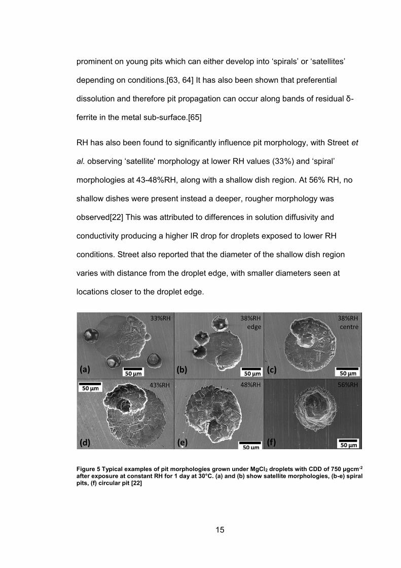
There are many iron oxides; the 9 most likely compounds to form during

atmospheric corrosion of stainless steel are outlined in Table 4[73].

Table 4 - Phases of rust, their formula and structure, information collated from Cornell & Schwertmann[73]

Name Formula Structure Colour Found in:

Goethite α-FeOOH Orthorhombic yellow-brown

rocks, soils

Akaganeite β-FeOOH Monoclinic bright yellow-brown

Chloride rich environments

Lepidocrocite γ-FeOOH Orthorhombic orange rocks, soil, biota, rust

Feroxyhyte δ’-FeOOH Hexagonal red-brown

‘various surface environments’

Hematite α-Fe2O3 Rhombohedral hexagonal

blood-red

soils, rocks

Maghemite γ-Fe2O3 Cubic or tetragonal

red-brown

Soils

Ferrihydrite Variable - Fe2O3·XH2O/ Fe5O8H.H2O

Hexagonal red-brown

streams, rivers, mud, soil, rock, all living things

Magnetite Fe3O4 Cubic black rocks, biota

Green rusts many, contains FeII and FeIII, Cl- and SO4

2-

Layered double hydroxide octahedral

green corrosion product

18

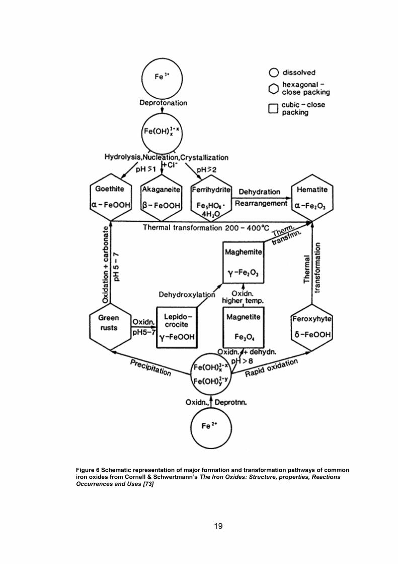
2.4.1 Formation and transformation of the iron oxides

Formation of an iron oxide or hydroxide phase is a well understood process and

occurs through either direct precipitation from a solution containing ferric (Fe3+)

or ferrous (Fe2+) ions or by transformation from another crystal phase, either by

dissolution and re-precipitation or by solid state transformation. The formation of

a particular species over another is heavily dependent on the pH, temperature,

rate of ion supply and presence of other local ions such as chloride or sulphate.

[73, 74] Figure 6 shows an overview of major formation pathways of various iron

oxides and oxide-hydroxides. Akaganeite (β-FeOOH) is of particular interest for

the high chloride concentration systems found in atmospheric environments as

it forms in acidic solutions above a threshold concentration of chloride ions,

which stabilise its ‘tunnel’ structure in the early stage of formation, despite not

being chemically included in compound.[73-75]

19

Figure 6 Schematic representation of major formation and transformation pathways of common iron oxides from Cornell & Schwertmann’s The Iron Oxides: Structure, properties, Reactions Occurrences and Uses [73]

20

Iron oxides are also well known for their propensity to transform into other

oxides and hydroxides[73], care therefore has to be taken to minimise the

possibility of transformation when performing characterisation techniques such

as Raman spectroscopy which can heat the sample and induce undesired

phase transformation, generally to hematite. [76-78]

2.4.2 Characterisation of iron oxides and oxide-hydroxides

Iron oxides and hydroxides have been characterised using various

spectroscopic techniques; micro-Raman spectroscopy has been extensively

utilised due to the ability to non-destructively discriminate between crystal

phases with a small sample volume. [79-84]

The UV-VIS-IR spectral region has been of interest for remote sensing of iron

oxides and oxide-hydroxides in earth and space science due the ability to use

ambient light to illuminate the sample, thus allowing for spectroscopy to be

performed from long distances (i.e. from aircraft or satellites)[85-87].

Sherman[88] et al. characterised the UV-VIS-IR diffuse reflectance spectra of

iron oxides and oxide-hydroxides from 350 nm-2150 nm for use in identifying

Martian minerals and assigns the 400 -1000 nm region as the ‘most diagnostic

spectral region for delineating the iron oxide phases’.

Mossbauer, XRD and micro-XRD have also been used, but generally in a

complementary context to verify sample powder purity, or for assessing physical

properties of powders such as size, crystallinity and packing density[77, 87, 89-

91]

21

2.4.3 Atmospheric corrosion products of iron alloys

Extensive work has been performed to characterise the corrosion products of

iron, both by controlled laboratory experiment [92, 93] and by evaluation of

corrosion products found on archaeological samples [81-83, 90, 94].

Dunnwald et al.[92] used Raman spectroscopy to investigate corrosion products

of iron after repeated wetting and drying of a 1 μm thin film of iron deposited on

gold substrate, they reported a cycle whereby goethite (α-FeOOH) and

lepidocrocite (γ-FeOOH) were formed, which would transform to Fe(OH)2 upon

rewetting and then Fe(OH)3 upon partial drying before crystallising to α or β-

FeOOH again. This cycle could then be broken by the subsequent reduction of

Fe(OH)2 and FeOOH to magnetite (Fe3O4) which would remain as the final

product. Dubois et al.[95] also observed magnetite, maghemite and goethite

under wet-dry cycling of NaCl salt spray in atmospheric conditions, with a

gradual transformation to akaganeite observed as more cycles are performed.

Raman spectroscopy has also been extensively used for characterisation of

atmospheric corrosion of corrosion products found on archaeological iron

samples, Bellot-Gurlet et al. and Monnier et al. [81, 82] studied samples of iron

chain from Amiens cathedral (1497), reporting layered corrosion products with

iron oxide-hydroxides goethite, lepidocrocite and akaganeite present. They

assign some spectra as ‘General poorly crystallised iron(III) oxide or oxide-

hydroxide’ due to poor signal to noise indicating a lack of crystallinity.

Bellot-Gurlet et al. and Neff et al. [81, 83] also studied corrosion products in

buried samples, seeing different corrosion products based on the level of

22

aeration of the soil, with Siderite (FeCO3) and magnetite in anoxic conditions

and a mix of goethite, maghemite and magnetite in aerated soils, along with

some siderite, iron hydroxychloride (β-Fe2(OH)3Cl) and akaganeite associated

with increased chloride and carbonate. Similarly, Shengxi et al. [90] studying

carbon steel samples immersed in seawater for ~60 years found a layer of iron

hydroxychloride, Fe3O4 and akaganeite covered in a layer of iron and calcium

carbonates. Réguer et al. [84] also reports increased volumes of akaganeite in

chloride rich environments.

“Green rusts” are also potential corrosion products of iron, they are generally

short lived and take the form of ‘layered double hydroxides’ in the hydrotalcite

super-group of minerals. They are a mix of hydroxide and carbonate groups

which include anions such as chloride and sulphate and have been known to

include others e.g. halogenides, perchlorate and nitrate.[73]. Legrand identified

an electrochemical method of producing chloride ‘GR1’ (green rust 1) and

characterised it with Raman spectroscopy.[96] Other, similar minerals exist,

such as pyroaurite, iowaite and coalingite within this group and can be

distinguished by their ratio of Fe3+ to Fe2+[97, 98].

2.4.4 Corrosion products of stainless steel

Some work has been done previously to characterise the product formed from

pitting on 304/316 stainless steel in atmospheric conditions. Luo et al[99]., Dong

et al. [100] and Dhaiveegan et al.[101] used a range of techniques including

Raman spectroscopy to characterise corrosion products. Luo, Dong and

Dhaiveegan studied the development of corrosion of 304L under atmospheric

conditions over a time period of several months, the environments were tropical,

23

marine and urban respectively. Ferreira’s samples were under full immersion of

0.15M NaCl. Luo, Dong and Ferreira observed similar Raman spectra; Ferreira

assigns goethite, chromium oxides and ‘a mixture of oxides and hydroxides

formed by atmospheric oxidation’ as the main constituents observed, whilst Luo

and Dong report a mixture of akaganeite, magnetite, maghemite and hematite.

Dhaiveegan was able to take multiple readings over a 36 month period and

noted the transformation of corrosion products between magnetite, hematite,

lepidocrocite and goethite across rainy seasons, which eventually stabilise to

goethite with a low amount of maghemite and akaganeite[101].

2.5 Corrosion detection and monitoring

Many industries routinely inspect for corrosion and so non-destructive

techniques have been developed to assess metal attack, some making use of

advanced equipment such as millimetre wave radar ultrasound and x ray

fluorescence[102] and others using simple visual and percussive-acoustic

assessment by a skilled inspector.[103-107] However, these are generally

operated manually and require contact or close proximity with the material being

tested.

Most remote sensing techniques that have involved image based corrosion

detection focused on either texture or colour based analysis [108-110]. These

have focused on detection of large areas of rust on carbon steel or for corrosion

related deformation of surfaces and will be explored further in the image

analysis section.

24

2.5.1 Principles of imaging and spectroscopy

All characterisation techniques used in this project take advantage of the

mechanisms by which light interacts with matter. Light is quantized, which is to

say that it behaves as discrete units or quanta, each of a specific energy given

by:

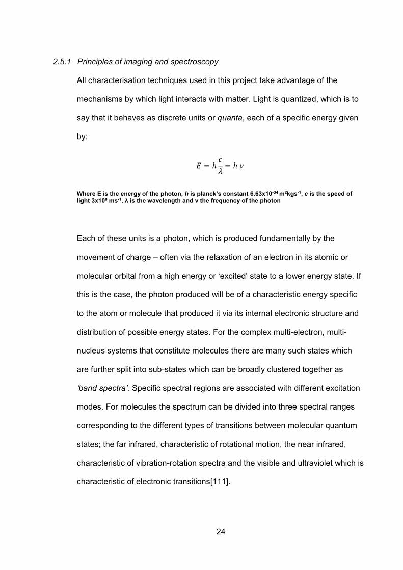
𝐸 = ℎ𝑐

𝜆= ℎ 𝜈

Where E is the energy of the photon, h is planck’s constant 6.63x10-34 m2kgs-1, c is the speed of light 3x108 ms-1, λ is the wavelength and ν the frequency of the photon

Each of these units is a photon, which is produced fundamentally by the

movement of charge – often via the relaxation of an electron in its atomic or

molecular orbital from a high energy or ‘excited’ state to a lower energy state. If

this is the case, the photon produced will be of a characteristic energy specific

to the atom or molecule that produced it via its internal electronic structure and

distribution of possible energy states. For the complex multi-electron, multi-

nucleus systems that constitute molecules there are many such states which

are further split into sub-states which can be broadly clustered together as

‘band spectra’. Specific spectral regions are associated with different excitation

modes. For molecules the spectrum can be divided into three spectral ranges

corresponding to the different types of transitions between molecular quantum

states; the far infrared, characteristic of rotational motion, the near infrared,

characteristic of vibration-rotation spectra and the visible and ultraviolet which is

characteristic of electronic transitions[111].

25

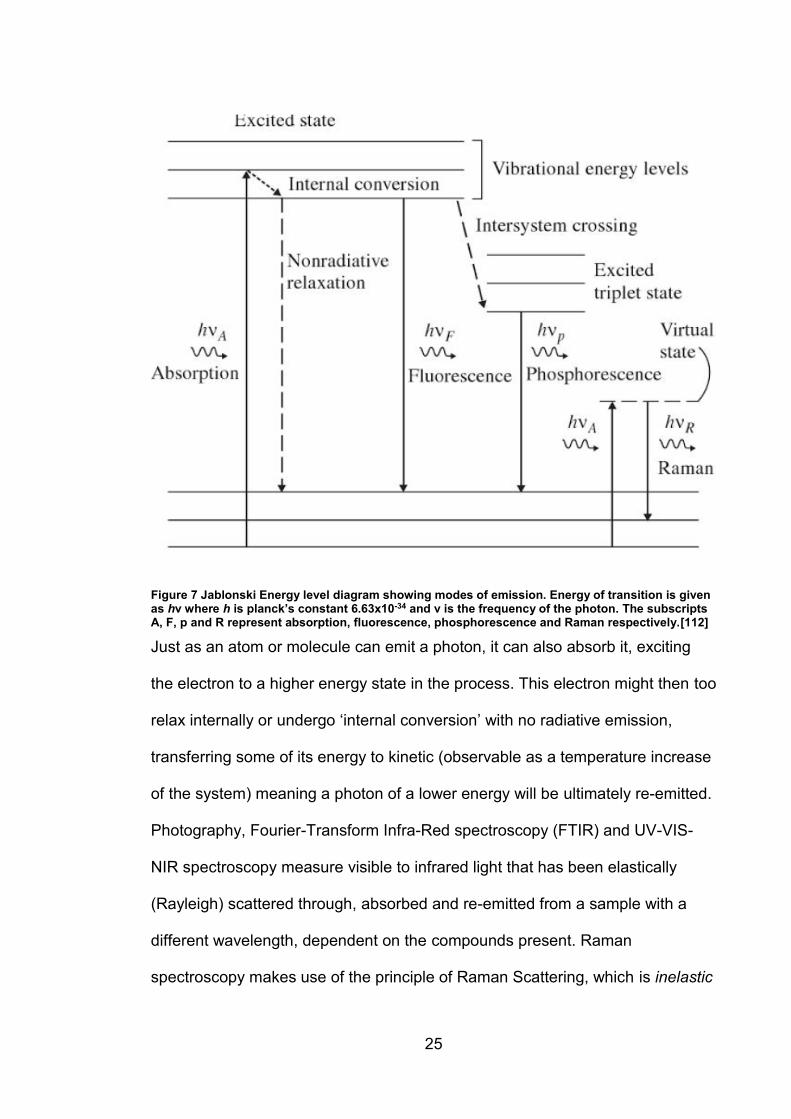
Figure 7 Jablonski Energy level diagram showing modes of emission. Energy of transition is given as hν where h is planck’s constant 6.63x10-34 and ν is the frequency of the photon. The subscripts A, F, p and R represent absorption, fluorescence, phosphorescence and Raman respectively.[112]

Just as an atom or molecule can emit a photon, it can also absorb it, exciting

the electron to a higher energy state in the process. This electron might then too

relax internally or undergo ‘internal conversion’ with no radiative emission,

transferring some of its energy to kinetic (observable as a temperature increase

of the system) meaning a photon of a lower energy will be ultimately re-emitted.

Photography, Fourier-Transform Infra-Red spectroscopy (FTIR) and UV-VIS-

NIR spectroscopy measure visible to infrared light that has been elastically

(Rayleigh) scattered through, absorbed and re-emitted from a sample with a

different wavelength, dependent on the compounds present. Raman

spectroscopy makes use of the principle of Raman Scattering, which is inelastic

26

scattering of incident light, with no resonant characteristic between incident light

and scattering molecule necessary (unlike fluorescence which requires

resonant absorption of incident light). For Raman scattering to occur, the

incident radiation must be monochromatic (frequency ν). The radiation scattered

at right angles to the incident direction will contain not only elastically (Rayleigh)

scattered light of frequency ν, but also much weaker radiation of frequency ν ±

ν’ of which ν’ is the Raman scattered component. A resulting spectrum of this

scattered light will not only have a strong monochromatic line of the illuminating

frequency ν, but weak ‘Raman’ lines either side of it which will be characteristic

of transitions in the scattering molecule.[111]

2.5.2 Hyperspectral imaging

Spectral images are obtained by gathering spectral information for each pixel in

an image of a scene, rather than a single intensity value. Hyperspectral imaging

is differentiated from multispectral imaging by having a regular spectral interval,

usually on the order of 1-10 nm rather than discrete, often irregular wavelength

points where intensity information is gathered. Data gathered is arranged in a

‘hypercube’, with spatial information in the x and y dimensions and spectral in

the z.

Hyperspectral imaging sees extensive use in industry and science; for example

in earth and extra planetary science for classifying and mapping foliage cover

and the extent of urbanisation around the world[113-116], for mineral

prospecting [4, 5, 85, 117], for characterising the surface minerology of planets

and asteroids[86, 118-121], agriculture for large scale assessment of crop

state[122], the food industry for assessing product quality[123], in the

27

preservation and restoration of archives and paintings for characterising inks

and paint pigments and also in medicine to diagnose cancers through imaging

blood via capillaries in the eye.[124]

Very little work has been done on hyperspectral imaging in a corrosion

detection context, but work in prospecting for iron ores using air and space-

borne spectral imaging sensors and for characterising the surface of earth and

mars are highly relevant as they aim to identify similar iron-bearing

mineralogy[3-5, 86, 115, 117-119, 125]. For example the OMEGA instrument

aboard the Mars express mission is used for identifying Martian surface

mineralogy, atmospheric aerosols and polar CO2 ice. They are able to generally

discriminate iron oxides from other minerals by a broad spectral band centred at

900 nm, but also report useful regions at 1900 nm and 2500 nm for identifying

hydration level of goethite [118, 125, 126]. Similarly the Landsat and EO-1

missions have been used for mineral prospecting of iron ores using the

multispectral Hyperion and orbital land imager instruments, using band ratios to

ascertain hematite-goethite ratio and thus abundance of Fe3+ and quality of

ore[127].

28

2.5.3 Image analysis

The process of extracting useful features from an image is critical to the

effectiveness of an imaging system, whether hyperspectral or a colour

photograph. The simplest method of doing this is thresholding, whereby an

intensity gradient is identified across the image and a threshold is applied to

separate the feature from the background. Due to the aforementioned diffuse

UV-VIS-NIR reflectance band at 650-900 nm which gives iron oxides and iron

oxide-hydroxides their characteristic red colouring[73, 80, 88], a natural

differential exists with which to segment images in a corrosion context.

Colour cameras measure intensity at three wavelength bands centered upon

approximately 450, 550 and 650 nm. These correspond to the colours blue,

green and red. When overlaid, these three colour ‘channels’ give an image

which is natural to visually interpret, however the raw data is not intuitive to

understand outside the representation of an image of a scene. For this reason,

colour-spaces have been developed to aid and simplify manipulation of colour

image data. Used in this project are the ‘HSV’ colour space and the ‘L*a*b*’

colour space.

29

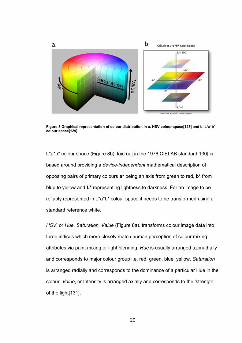
Figure 8 Graphical representation of colour distribution in a. HSV colour space[128] and b. L*a*b* colour space[129]

L*a*b* colour space (Figure 8b), laid out in the 1976 CIELAB standard[130] is

based around providing a device-independent mathematical description of

opposing pairs of primary colours a* being an axis from green to red, b* from

blue to yellow and L* representing lightness to darkness. For an image to be

reliably represented in L*a*b* colour space it needs to be transformed using a

standard reference white.

HSV, or Hue, Saturation, Value (Figure 8a), transforms colour image data into

three indices which more closely match human perception of colour mixing

attributes via paint mixing or light blending. Hue is usually arranged azimuthally

and corresponds to major colour group i.e. red, green, blue, yellow. Saturation

is arranged radially and corresponds to the dominance of a particular Hue in the

colour. Value, or Intensity is arranged axially and corresponds to the ‘strength’

of the light[131].

30

Colour segmentation of images is used extensively in industry for machine

vision applications such as high throughput produce quality assessment and

sorting. [132-134] Some work has been done with the aim of developing image

processing based corrosion detection systems: Itzhak et al. were first to employ

image processing by intensity thresholding greyscale images of pitting on 304

stainless steel in a 10%FeCl3 solution with the aim of developing statistical

analysis tools for evaluating total pitted are of a metal surface. Due to the full

immersion conditions producing little rust, segmentation highlighted deformation

of the pitted metal surface rather than corrosion products. [135] This is

expanded on by Choi et al. who combine several texture and colour properties

of the pitted metal surface to classify corrosion damage.[136] Medeiros et al.

use a similar multi-descriptor based approach for corrosion detection on carbon

steel, this time imaging the corrosion product rather than the metal surface

before performing Fisher linear discriminant analysis (FLDA) [110], similarly

Valeti outlined a procedure for colour based corrosion detection in L*a*b* space

using k-means clustering [137]. Feliciano et. Al. have investigated a solely

texture based approach on A36 steel to assess the development of corrosion

over time.[138]

Principal Component Analysis is extensively made use of as a dimensionality

reduction and feature extraction method for hyperspectral imaging due to its

ability to easily organize data down lines of maximum variance and quickly

optimize a dataset for viewing[139-142]. It has similarly been used for

unsupervised feature extraction of colour images with some success[143, 144]

31

and was also used as a pre-processing step before FLDA during Medeiros et

al’s corrosion detection work on carbon steel[110] .

32

2.6 Summary

Atmospheric pitting corrosion of stainless steel is an indicator of risk of AISSC,

which could cause failure in containers when they come to be moved to

permanent disposal in a GDF. It is caused by the deliquescence of aerosol salt

particles to form a concentrated solution. Pitting leaves a deposit of rust which

could be used to indicate the presence of a corrosion site.

Hyperspectral imaging is extensively made use of in industry and science for

detection and quantification of iron oxide species, but has yet to be applied to

corrosion monitoring. Extensive work has been undertaken to characterise iron

oxide products of corrosion products using Raman spectroscopy and while

some techniques have been developed for detecting corrosion using

photography and image processing, little work has specifically targeted pitting

corrosion.

The aims of this Thesis are:

To identify the specific corrosion products present on 304L stainless

steel during pitting corrosion

Evaluate the effect of droplet chemistry on these corrosion products in

stores relevant conditions

Determine the optimum imaging and analysis methods for quantifying

visible rust

Use this method to investigate the relationship between corrosion pit

volume and visible rust.

33

3. Methodology

3.1 Droplet experiments

3.1.1 Materials and sample preparation

All droplet experiments were performed on 3 mm thick 304L stainless steel

(Aperam-France, Table 5) which had been cold-rolled and solution treated at

1040-1100°C before undergoing forced air cooling by the manufacturer. The

plate was received in 250 x 250 mm plates.

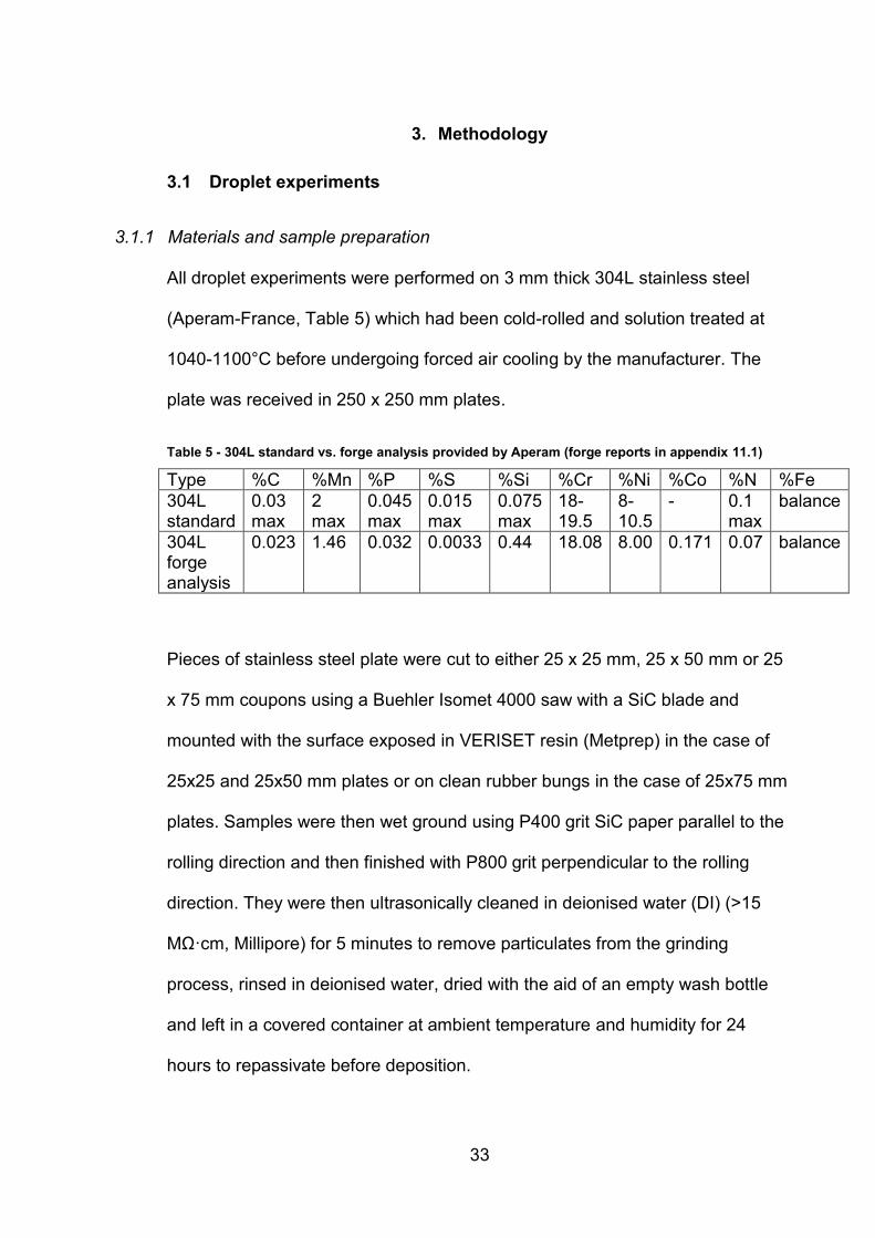
Table 5 - 304L standard vs. forge analysis provided by Aperam (forge reports in appendix 11.1)

Type %C %Mn %P %S %Si %Cr %Ni %Co %N %Fe

304L standard

0.03 max

2 max

0.045 max

0.015 max

0.075 max

18-19.5

8-10.5

- 0.1 max

balance

304L forge analysis

0.023 1.46 0.032 0.0033 0.44 18.08 8.00 0.171 0.07 balance

Pieces of stainless steel plate were cut to either 25 x 25 mm, 25 x 50 mm or 25

x 75 mm coupons using a Buehler Isomet 4000 saw with a SiC blade and

mounted with the surface exposed in VERISET resin (Metprep) in the case of

25x25 and 25x50 mm plates or on clean rubber bungs in the case of 25x75 mm

plates. Samples were then wet ground using P400 grit SiC paper parallel to the

rolling direction and then finished with P800 grit perpendicular to the rolling

direction. They were then ultrasonically cleaned in deionised water (DI) (>15

MΩ·cm, Millipore) for 5 minutes to remove particulates from the grinding

process, rinsed in deionised water, dried with the aid of an empty wash bottle

and left in a covered container at ambient temperature and humidity for 24

hours to repassivate before deposition.

34

3.1.2 Solution preparation

Bulk 0.044 M MgCl2 and CaCl2 solutions were prepared from MgCl2·6H2O or

CaCl2 salt (Sigma Aldrich) using DI water (>15 MΩ·cm, Millipore), which

corresponded to ~100 μgcm-2 chloride deposition density (CDD) with a 4μL

droplet. When a lower chloride deposition density was required, serial dilution

was used to create a solution of the appropriate concentration; 0.022 μL for a

CDD of 50 μgcm-2 and 0.00088 μL for 20 μgcm-2.

35

3.1.3 Droplet deposition

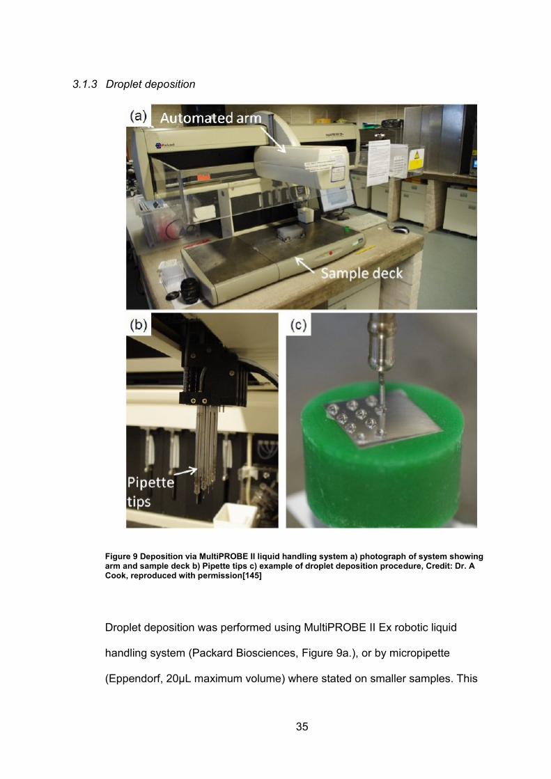
Figure 9 Deposition via MultiPROBE II liquid handling system a) photograph of system showing arm and sample deck b) Pipette tips c) example of droplet deposition procedure, Credit: Dr. A Cook, reproduced with permission[145]

Droplet deposition was performed using MultiPROBE II Ex robotic liquid

handling system (Packard Biosciences, Figure 9a.), or by micropipette

(Eppendorf, 20μL maximum volume) where stated on smaller samples. This

36

allowed for a large number of droplets of consistent volume and location to be

deposited in a short amount of time.[145] The system consists of a robot arm

which moves a pipette tip (Figure 9b), fed by an automated syringe. Hydraulic

action of ‘system liquid’ (DI water) is used to aspirate and dispense aqueous

solutions. An air gap is kept between the solution and the system liquid at all

times and the system is flushed with DI water when switching between

solutions.

Droplets were deposited in grids with an interval depending on experimental

requirement, but of no less than 2 mm between droplets (Figure 9c).

4 μL droplets were used for all experiments which consistently spread to a

radius of approximately 2 mm on the finished sample surface.[63] This allowed

chloride deposition density to be controlled by deposition of solution of known

concentration alone; 0.044 μLfor a CDD of 100 μgcm-2, 0.022 μL for 50 μgcm-2

and 0.00088 μL for 20 μgcm-2.

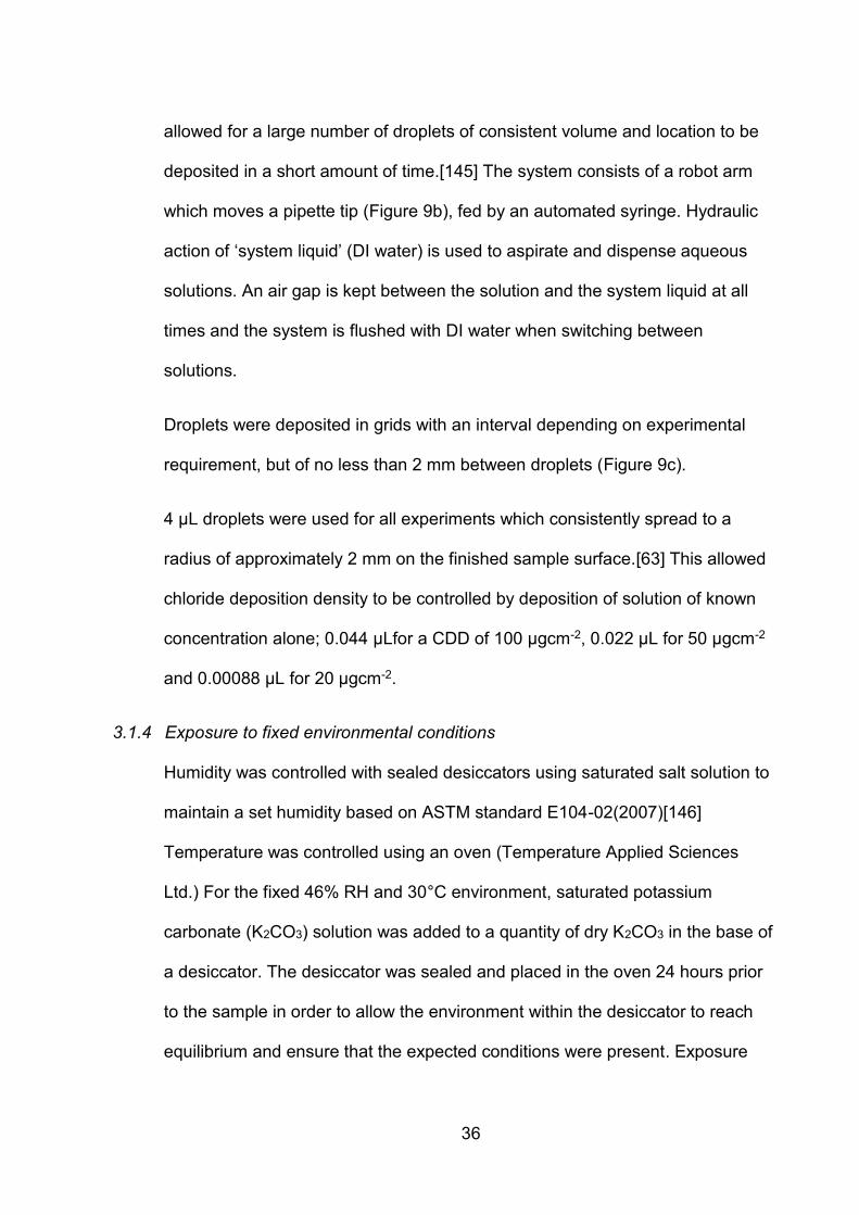
3.1.4 Exposure to fixed environmental conditions

Humidity was controlled with sealed desiccators using saturated salt solution to

maintain a set humidity based on ASTM standard E104-02(2007)[146]

Temperature was controlled using an oven (Temperature Applied Sciences

Ltd.) For the fixed 46% RH and 30°C environment, saturated potassium

carbonate (K2CO3) solution was added to a quantity of dry K2CO3 in the base of

a desiccator. The desiccator was sealed and placed in the oven 24 hours prior

to the sample in order to allow the environment within the desiccator to reach

equilibrium and ensure that the expected conditions were present. Exposure

37

conditions were verified by EasyLog EL-USB-2-LCD (Lascar Electronics Ltd.)

with an accuracy of ±0.5°C and ±3% RH.

3.1.5 Exposure to fluctuating ambient environmental conditions

Samples described as exposed to fluctuating ambient conditions were exposed

in desiccators which were left covered but not sealed to ensure equilibrium with

the environment whilst minimising the chance of unintended additional

deposition of atmospheric contaminants. Exposure conditions were recorded

and verified by EasyLog EL-USB-2-LCD data logger (Lascar Electronics Ltd.

with an accuracy of ±0.5°C and ±3% RH.

38

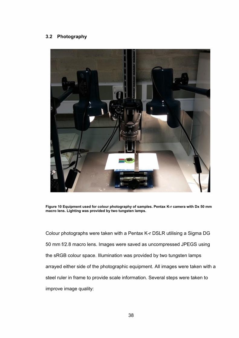
3.2 Photography

Figure 10 Equipment used for colour photography of samples. Pentax K-r camera with Dx 50 mm macro lens. Lighting was provided by two tungsten lamps.

Colour photographs were taken with a Pentax K-r DSLR utilising a Sigma DG

50 mm f/2.8 macro lens. Images were saved as uncompressed JPEGS using

the sRGB colour space. Illumination was provided by two tungsten lamps

arrayed either side of the photographic equipment. All images were taken with a

steel ruler in frame to provide scale information. Several steps were taken to

improve image quality:

39

1. All images were taken at the minimum focal distance of the lens,

maximising the size of the sample area on screen

2. Samples were oriented such that the grinding direction was horizontal on

the photograph. This minimised reflection from the light sources from

ridges in the grinding pattern and ensured uniformity of lighting in the

photograph.

3. Photographs were taken on aperture priority mode with the aperture

setting at f/2.8 to maximise sharpness of the image.

4. All additional camera post-processing was disabled

3.3 Iron oxide syntheses

Iron oxides and oxide-hydroxides were synthesised by Dr. Rowena Fletcher-

Wood using procedures provided by Cornell and Schwertmann.[73] Individual

procedures for each oxide and oxide-hydroxide crystal phase are outlined in

Appendix 11.2.

40

3.4 Characterisation and Spectroscopy

3.4.1 X-ray diffraction

A Bruker D2 PHASER was used to gather XRD data, which operates with a Co

source, and thus does not cause Fe and Mn to fluoresce. This instrument is run

in Lynxeye reflection mode. λ = 1.79026 A. The tube operates under 30 kV/10

mA acceleration, producing Co Kα-1 radiation. Samples were loaded into a

cavity and the surface flattened with a slide and analysed for 1 hour per sample

at a range of 5-80 o.

3.4.2 UV-VIS-NIR spectroscopy

UV-VIS-NIR diffuse reflectance spectra were gathered using an Oceanoptics

“Flame” UV-VIS-NIR spectrometer, with an Oceanoptics HL-2000 series

tungsten-halogen light source. Spectra were gathered using a probe consisting

of two optical fibres which guided light from the source to the sample and

reflected light back to the spectrometer. Instrument control and analysis was

performed using the “Oceanview” analysis software provided with the

instrument. Measurements were taken of the powdered samples deposited on a

glass slide with a gently tamped surface. The fibre probe was clamped

approximately 2 cm above the sample while measurement was performed.

Bright and dark field spectra for correction were taken of SPECTRALON 99%

and 2% calibrated reflectance standards. All measurements were taken in a

dark room to eliminate visible spectrum interference from lighting,

41

3.4.3 Fourier-Transform Infra-Red (FTIR) spectroscopy

FTIR spectroscopy was performed using a Thermo scientific Nicolet 8700

Model 912A0685. Samples were suspended in KBr, which was dried overnight

at 120°C. 300 mg of KBr was used per 3 g of sample.

42

3.4.4 Raman Spectroscopy

A Renishaw InVia spectrometer with confocal microscope was used to identify

corrosion products after exposure. The wavelength of the excitation laser was

488 nm and the maximum estimated power output after optical losses was 20

mW. All spectroscopy was performed through a 20x super long working

distance objective, giving a spot size of approximately 10 μm. In order to

prevent the thermal transformation of corrosion iron oxide-hydroxide corrosion

products laser power was limited to 10% of maximum (~2 mW). Each

measurement was the product of 30 accumulations of 10 seconds each (unless

otherwise specified), giving a total per-measurement acquisition time of 5

minutes. The data range was measured from 50 – 1600 cm-1. The instrument

was controlled using Renishaw’s WiRE software version 4.0. No sample

preparation such as rinsing of salt solution or corrosion product off the sample

surface was performed and measurements did not take place under RH or

temperature control due to equipment limitations.

3.4.4.1 Raman spectroscopic mapping

Mapping data was collected by automated acquisition of multiple point

measurements in a grid across the sample surface with the total number of

points and interval between measurements dictated by the size of the sample

and instrument time available for acquisition. Each pixel in the final map

therefore constitutes an individual spectrum from the acquisition. Due to the

long acquisition time necessitated by preventing thermal transformation of

corrosion product species, the total acquisition time for a map was the limiting

43

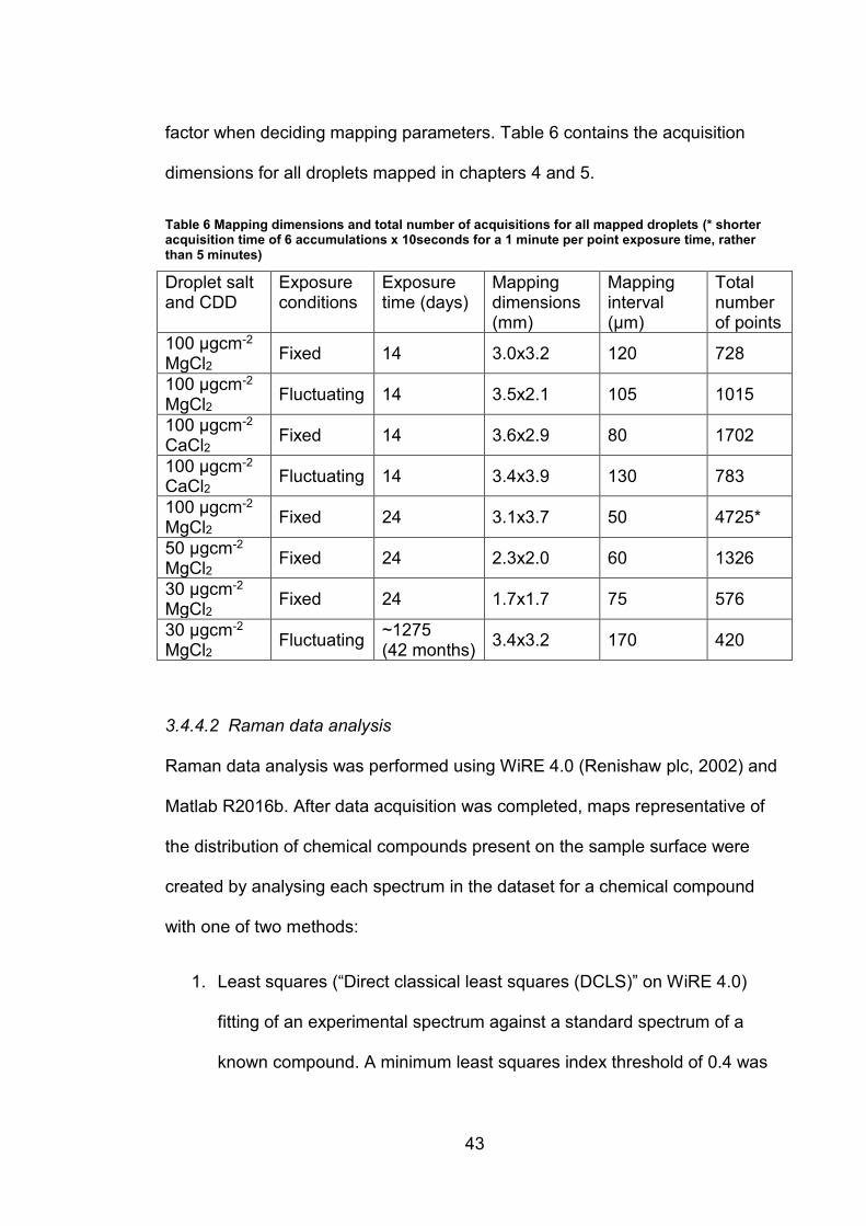
factor when deciding mapping parameters. Table 6 contains the acquisition

dimensions for all droplets mapped in chapters 4 and 5.

Table 6 Mapping dimensions and total number of acquisitions for all mapped droplets (* shorter acquisition time of 6 accumulations x 10seconds for a 1 minute per point exposure time, rather than 5 minutes)

Droplet salt and CDD

Exposure conditions

Exposure time (days)

Mapping dimensions (mm)

Mapping interval (μm)

Total number of points

100 μgcm­2 MgCl2 Fixed 14 3.0x3.2 120 728

100 μgcm­2 MgCl2

Fluctuating 14 3.5x2.1 105 1015

100 μgcm­2

CaCl2 Fixed 14 3.6x2.9 80 1702

100 μgcm­2

CaCl2 Fluctuating 14 3.4x3.9 130 783

100 μgcm­2

MgCl2 Fixed 24 3.1x3.7 50 4725*

50 μgcm­2

MgCl2 Fixed 24 2.3x2.0 60 1326

30 μgcm­2

MgCl2 Fixed 24 1.7x1.7 75 576

30 μgcm­2

MgCl2 Fluctuating

~1275 (42 months)

3.4x3.2 170 420

3.4.4.2 Raman data analysis

Raman data analysis was performed using WiRE 4.0 (Renishaw plc, 2002) and

Matlab R2016b. After data acquisition was completed, maps representative of

the distribution of chemical compounds present on the sample surface were

created by analysing each spectrum in the dataset for a chemical compound

with one of two methods:

1. Least squares (“Direct classical least squares (DCLS)” on WiRE 4.0)

fitting of an experimental spectrum against a standard spectrum of a

known compound. A minimum least squares index threshold of 0.4 was

44

used for compound assignment. All iron oxide-hydroxide phases were

fitted for in this manner.

2. Index thresholding of a wavenumber to find the distribution of a single

peak. The threshold intensity was 150 unless otherwise stated. This was

performed if an unknown spectrum was observed.

After a map had been created, all spectra associated with said map were

averaged to improve the signal to noise ratio using the script provided in

Appendix 11.3

3.5 UV-VIS-NIR Hyperspectral Imaging

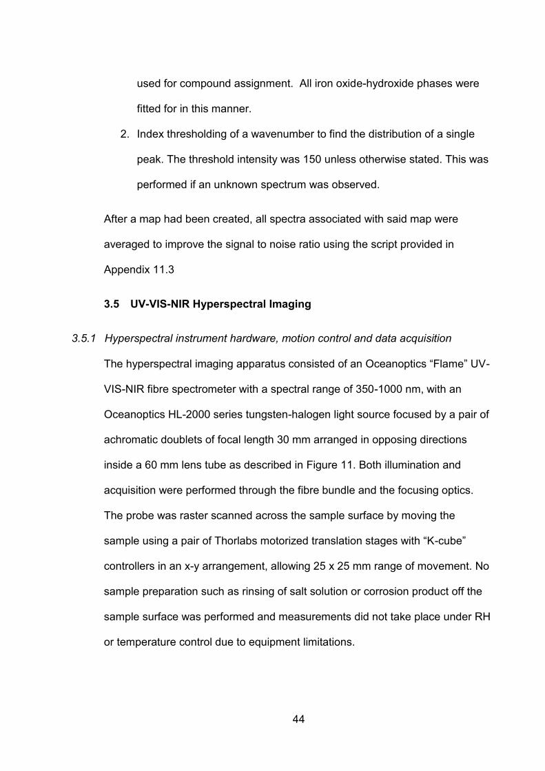
3.5.1 Hyperspectral instrument hardware, motion control and data acquisition

The hyperspectral imaging apparatus consisted of an Oceanoptics “Flame” UV-

VIS-NIR fibre spectrometer with a spectral range of 350-1000 nm, with an

Oceanoptics HL-2000 series tungsten-halogen light source focused by a pair of

achromatic doublets of focal length 30 mm arranged in opposing directions

inside a 60 mm lens tube as described in Figure 11. Both illumination and

acquisition were performed through the fibre bundle and the focusing optics.

The probe was raster scanned across the sample surface by moving the

sample using a pair of Thorlabs motorized translation stages with “K-cube”

controllers in an x-y arrangement, allowing 25 x 25 mm range of movement. No

sample preparation such as rinsing of salt solution or corrosion product off the

sample surface was performed and measurements did not take place under RH

or temperature control due to equipment limitations.

45

Figure 11 Schematic representation of hyperspectral imaging equipment showing arrangement of focusing optics and light path.

Spectra were acquired at set intervals across the sample surface, forming a

hyperspectral image whereby each spectrum constituted a pixel. Integration

time was set at 6500 µs for all spectral acquisitions. Focusing was performed to

maximise returned signal from the sample surface before acquisition using a

Thorlabs PT1B manual z stage mounted vertically.

The instrument was controlled by laptop via USB. Labview was used to

integrate motion control with spectral acquisition, the program is provided with

supplemental data attached to this document. Each hyperspectral image was

output as a comma separated text file and processed using Matlab R2017b.

Scripts for processing can be found in Appendix 11.4.

46

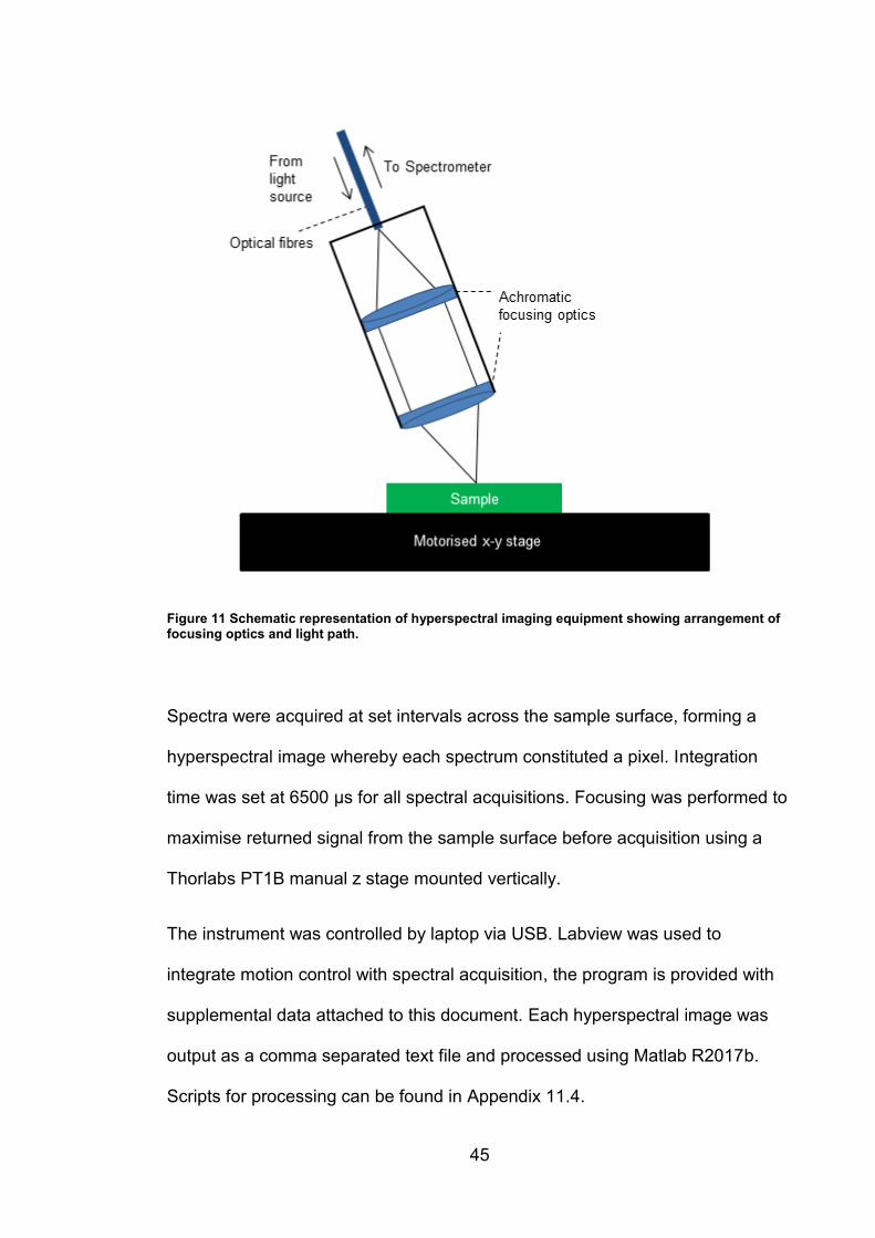
3.5.1.1 Flat field correction

Flat field correction was performed on all experimental and standard

acquisitions unless otherwise stated. This was done for an x by y (spatial) by n

(spectral) hyperspectral image matrix I using:

𝐼𝑐𝑜𝑟𝑟𝑒𝑐𝑡𝑒𝑑 =𝐼𝑟𝑎𝑤 − 𝐼𝑑𝑎𝑟𝑘

𝐼𝑏𝑟𝑖𝑔ℎ𝑡 − 𝐼𝑑𝑎𝑟𝑘

Equation 1 Where Icorrected is the final hyperspectral image, Iraw is the raw hyperspectral image, Idark and Ibright are single spectra of 2% and 99% spectralon reflectance standards respectively as the dark and bright field

Ibright and Idark were 1xn spectra averaged from hyperspectral images of 2x2 mm

areas of 99% and 2% spectralon calibrated reflectance tiles (Figure 13). The

spectra were reacquired at the beginning of every experimental session.

47

3.5.2 Characterisation of UV-VIS hyperspectral imaging system

3.5.2.1 Resolution characterisation

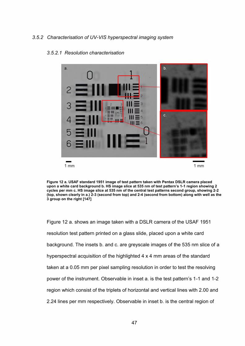
Figure 12 a. USAF standard 1951 image of test pattern taken with Pentax DSLR camera placed upon a white card background b. HS image slice at 535 nm of test pattern’s 1-1 region showing 2 cycles per mm c. HS image slice at 535 nm of the central test patterns second group, showing 2-2 (top, shown clearly in a.) 2-3 (second from top) and 2-4 (second from bottom) along with well as the 3 group on the right [147]

Figure 12 a. shows an image taken with a DSLR camera of the USAF 1951

resolution test pattern printed on a glass slide, placed upon a white card

background. The insets b. and c. are greyscale images of the 535 nm slice of a

hyperspectral acquisition of the highlighted 4 x 4 mm areas of the standard

taken at a 0.05 mm per pixel sampling resolution in order to test the resolving

power of the instrument. Observable in inset a. is the test pattern’s 1-1 and 1-2

region which consist of the triplets of horizontal and vertical lines with 2.00 and

2.24 lines per mm respectively. Observable in inset b. is the central region of

48

the test pattern with regions 2-1 to 2-4 present on the left hand side of the

image at 4.00 to 5.66 cycles per mm. 3-1 to 3-6 are present on the right hand

side (partially obscured by image edge) with 8.00 - 14.3 lines per mm. Regions

4 to 7 are present in the lower half of the image between regions 2 and 4, but

are unresolvable. A full list of cyclic resolution values can be found in Table 7.

Table 7 Reproduction of table included with 1951 USAF test pattern showing the resolution values for markings present[147]

RESOLUTION VALUES FOR STANDARD USAF 1951 RESOLUTION TEST

PATTERN

(All values in Cycles Per Millimeter)

GROUPS

ELEMENTS -2 -1 0 1 2 3 4 5 6 7

1 .250 .500 1.00 2.00 4.00 8.00 16.0 32.0 64.0 128

2 .281 .561 1.12 2.24 4.49 8.98 17.9 35.9 71.8 143

3 .315 .629 1.26 2.52 5.04 10.1 20.1 40.3 80.6 161

4 .354 .707 1.41 2.83 5.66 11.3 22.6 45.3 90.5 181

5 .397 .794 1.59 3.17 6.35 12.7 25.4 50.8 101 203

6 .445 .891 1.78 3.56 7.13 14.3 28.5 57.0 114 228

49

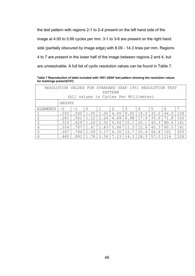
3.5.2.2 Instrument response function characterisation

Figure 13 Spectral responses used for flat field correction, taken using a. 99% SPECTRALON diffuse reflectance standard and b. 2% SPECTRALON diffuse reflectance standard. No flat field correction was applied

Figure 13 shows averages of a 2 x 2 mm area of a. 99% and b. 2% calibrated

reflectance standards taken at a sampling resolution of 0.2 mm per pixel,

showing combined spectral responses of the light source, fibre, focusing optics

and spectrometer. These spectra were used for flat field correction of all other

images in this chapter using Equation 1. The highest intensity is in the 450 nm-

850 nm wavelength interval, which is where the light source is brightest and the

optics most transmissive. This is therefore where the signal to noise ratio will be

highest. Subsequent spectral acquisitions will be trimmed to this wavelength

interval.

50

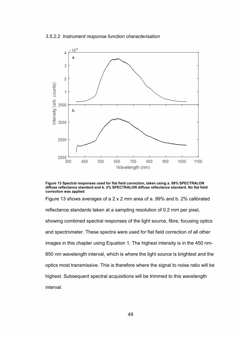
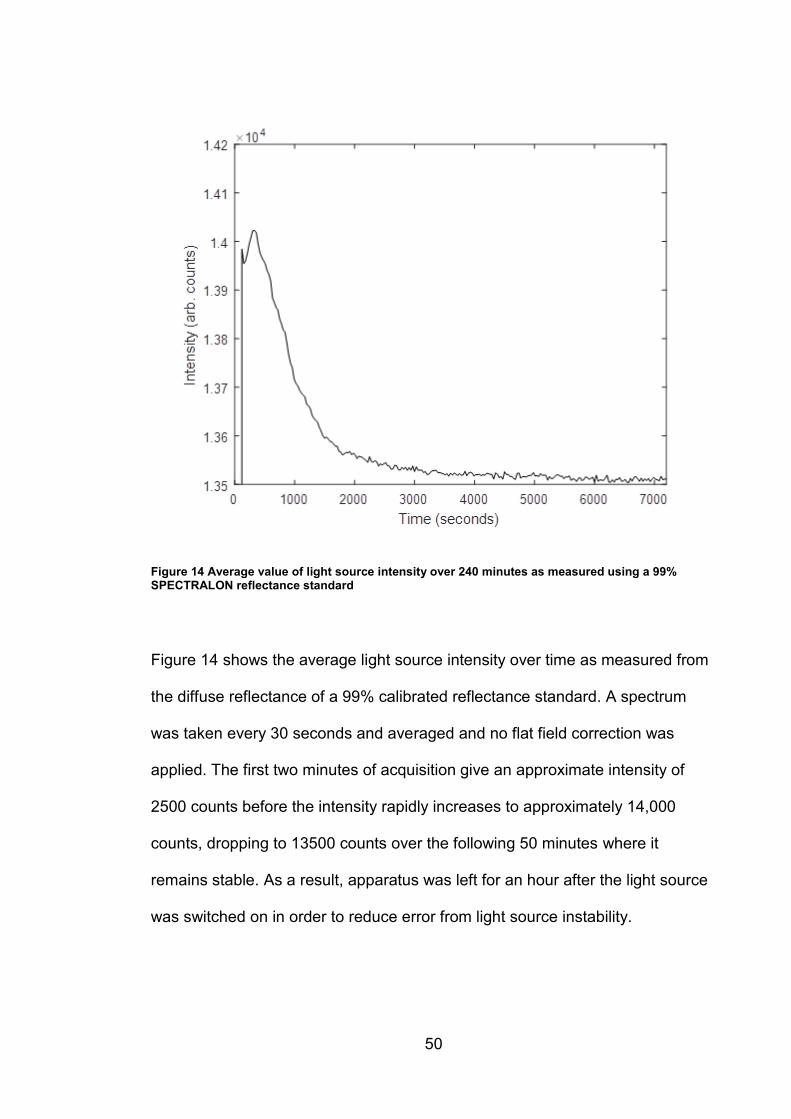
Figure 14 Average value of light source intensity over 240 minutes as measured using a 99% SPECTRALON reflectance standard

Figure 14 shows the average light source intensity over time as measured from

the diffuse reflectance of a 99% calibrated reflectance standard. A spectrum

was taken every 30 seconds and averaged and no flat field correction was

applied. The first two minutes of acquisition give an approximate intensity of

2500 counts before the intensity rapidly increases to approximately 14,000

counts, dropping to 13500 counts over the following 50 minutes where it

remains stable. As a result, apparatus was left for an hour after the light source

was switched on in order to reduce error from light source instability.

51

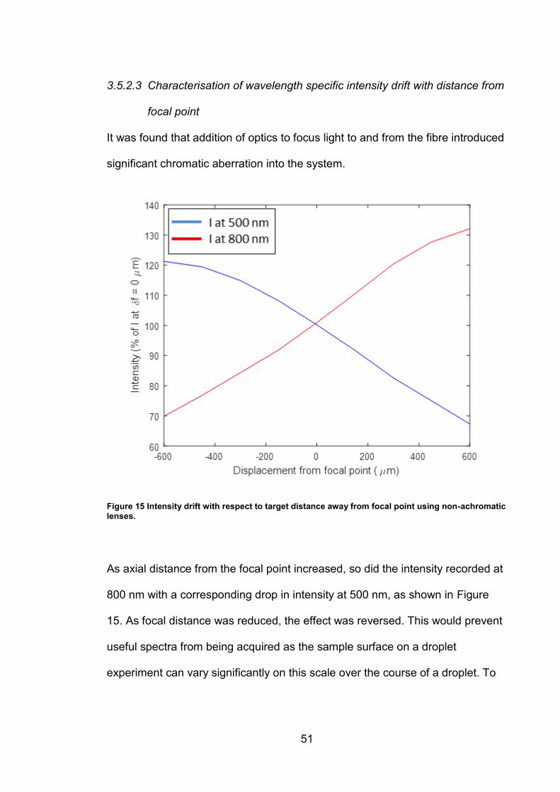
3.5.2.3 Characterisation of wavelength specific intensity drift with distance from

focal point

It was found that addition of optics to focus light to and from the fibre introduced

significant chromatic aberration into the system.

Figure 15 Intensity drift with respect to target distance away from focal point using non-achromatic lenses.

As axial distance from the focal point increased, so did the intensity recorded at

800 nm with a corresponding drop in intensity at 500 nm, as shown in Figure

15. As focal distance was reduced, the effect was reversed. This would prevent

useful spectra from being acquired as the sample surface on a droplet

experiment can vary significantly on this scale over the course of a droplet. To

52

combat this chromatic aberration in the instrument, the lenses present in the

focusing optics were replaced with achromatic lenses.

Figure 16 Intensity drift relative to a calibrated 75% reflectance standard as distance from focal point increases by wavelength after focusing optics were replaced with achromatic lenses.

Figure 16 shows chromatic intensity drift relative to a maximum at 0

displacement, indicating that intensity drops uniformly with axial displacement

from the focal point. The system was focused by shifting the assembly such that

the absolute intensity reflected from a 99% reflectance tile was maximized.

Reference spectra of 99% and 2% standards were then taken before and used

to correct subsequent spectra. Spectra were taken of a 75% reflectance

standard at displacements away from the focal point ranging from -750 µm to

+750 µm in increments of 150 µm. Spectra were the average of a 2 x 2 mm

53

area taken at an interval of 0.2 mm per acquisition. Intensity values are shown

for several wavelengths as a decimal of the intensity of the 99% reflectance

standard used for calibration. It should be noted that the corrected 75%

reflectance standard consistently produces a spectrum of 80 - 85% reflectance

rather than the expected 75%. Slight chromatic aberration is present above

+200 μm, seen as converging lines, but this is not significant enough to

compromise the ability to gather spectra on rough surfaces. Of note is ~5%

lower than expected intensity at -150 μm displacement, this does not

compromise the spectral response as a whole.

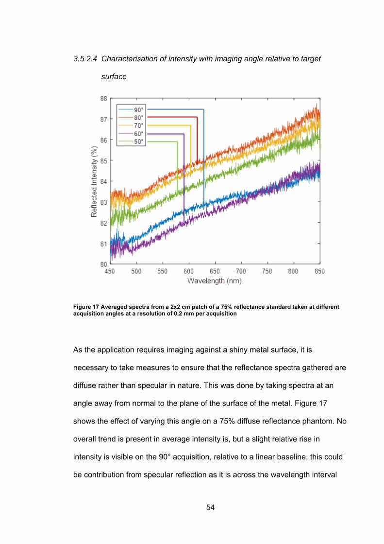
54

3.5.2.4 Characterisation of intensity with imaging angle relative to target

surface

Figure 17 Averaged spectra from a 2x2 cm patch of a 75% reflectance standard taken at different acquisition angles at a resolution of 0.2 mm per acquisition

As the application requires imaging against a shiny metal surface, it is

necessary to take measures to ensure that the reflectance spectra gathered are

diffuse rather than specular in nature. This was done by taking spectra at an

angle away from normal to the plane of the surface of the metal. Figure 17

shows the effect of varying this angle on a 75% diffuse reflectance phantom. No

overall trend is present in average intensity is, but a slight relative rise in

intensity is visible on the 90° acquisition, relative to a linear baseline, this could

be contribution from specular reflection as it is across the wavelength interval

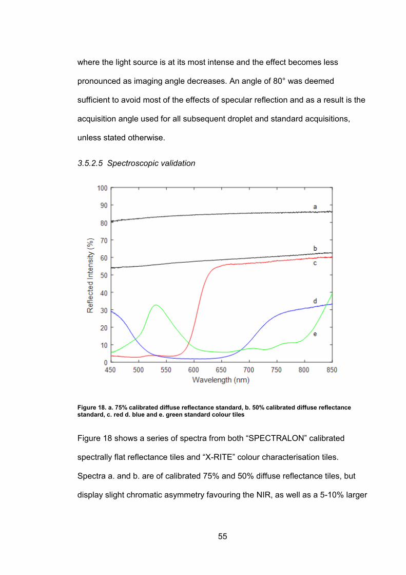
55

where the light source is at its most intense and the effect becomes less

pronounced as imaging angle decreases. An angle of 80° was deemed

sufficient to avoid most of the effects of specular reflection and as a result is the

acquisition angle used for all subsequent droplet and standard acquisitions,

unless stated otherwise.

3.5.2.5 Spectroscopic validation

Figure 18. a. 75% calibrated diffuse reflectance standard, b. 50% calibrated diffuse reflectance standard, c. red d. blue and e. green standard colour tiles

Figure 18 shows a series of spectra from both “SPECTRALON” calibrated

spectrally flat reflectance tiles and “X-RITE” colour characterisation tiles.

Spectra a. and b. are of calibrated 75% and 50% diffuse reflectance tiles, but

display slight chromatic asymmetry favouring the NIR, as well as a 5-10% larger

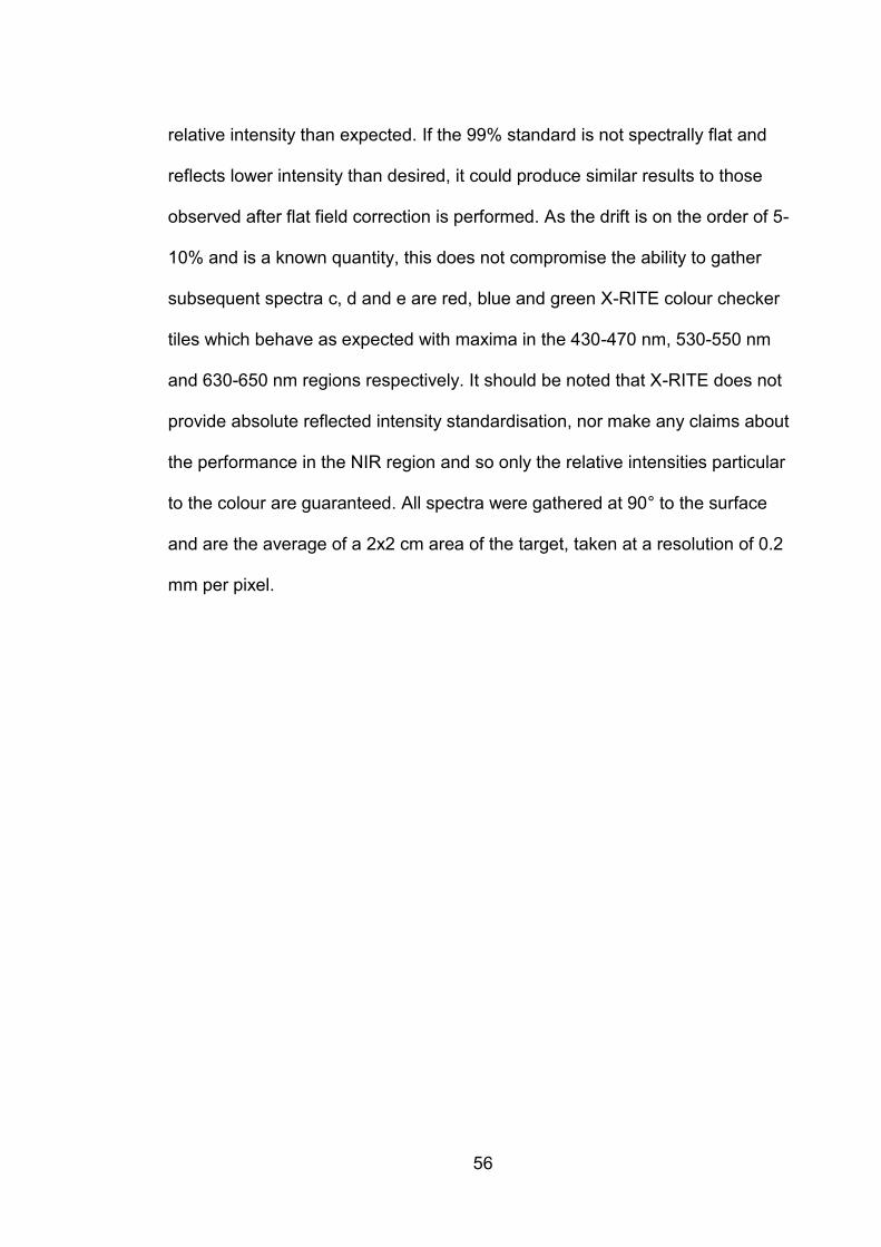
56

relative intensity than expected. If the 99% standard is not spectrally flat and

reflects lower intensity than desired, it could produce similar results to those

observed after flat field correction is performed. As the drift is on the order of 5-

10% and is a known quantity, this does not compromise the ability to gather

subsequent spectra c, d and e are red, blue and green X-RITE colour checker

tiles which behave as expected with maxima in the 430-470 nm, 530-550 nm

and 630-650 nm regions respectively. It should be noted that X-RITE does not

provide absolute reflected intensity standardisation, nor make any claims about

the performance in the NIR region and so only the relative intensities particular

to the colour are guaranteed. All spectra were gathered at 90° to the surface

and are the average of a 2x2 cm area of the target, taken at a resolution of 0.2

mm per pixel.

57

3.6 Rust area analysis

Figure 19 Flowchart of the procedure for extracting rust areas associated with individual corrosion sites from a colour photograph using the principal component analysis method

Semi-automated high-throughput rust area analysis was performed on colour

photographs using Matlab R2017b[148]. Scripts used can be found in

Appendices 11.4 and 11.5. Figure 19 shows the process for extracting rust

areas from corrosion sites using the principal component analysis (PCA)

segmentation technique, the full procedure is as follows:

1. Images were segmented using one of four techniques outlined below in

sections 3.6.1 to 3.6.4 in order to separate ‘rust’ pixels from ‘non-rust’

pixels (Figure 19 shows segmentation via the 2nd principal component.

58

2. Connected component analysis was performed to group neighbouring

pixels into individual ‘sites’, using the ‘bwconncomp’ function[148]

3. Sites with less than 100 pixels were discarded.

4. Almost-connected component analysis was used to group neighbouring

sites (distance of less than 50 pixels from its nearest neighbour) and

label individual corrosion sites.

5. The number of pixels associated with each corrosion site was then

extracted and converted to an area by multiplication by the average pixel

dimensions as determined from the scale photographed alongside the

sample.

3.6.1 Red-Blue colour channel subtraction

The RGB colour image is separated into its constituent colour channels and the

red channel is subtracted from the blue, before thresholding to produce the

segmented image. Matlab code for this procedure can be found in Appendix

11.5.1

3.6.2 Principal component analysis

Principal component analysis was performed on the data; the second principal

component is then thresholded to produce the segmented image. Matlab code

for this procedure can be found in appendix 11.5.2

3.6.3 HSV thresholding

The image is converted to HSV colour space from sRGB using the Matlab

standard “rgb2hsv” function before thresholds are then applied in hue and

saturation. Matlab code for this procedure can be found in Appendix 11.5.3

59

3.6.4 L*a*b* thresholding

The image is converted to L*a*b* colour space from sRGB using the Matlab

standard “rgb2lab” function with the ‘d65’ standard white point. A threshold is

then applied in b*. Matlab code for this procedure can be found in appendix

11.5.4

60

3.7 Confocal microscopy for pit volume measurement

Pit volumes measurements were performed using an Olympus LEXT OLS-4000

confocal laser scanning microscope. 3D measurements were taken by

sequentially scanning vertical sections of the sample which were reconstructed

by the software to a 3D volume. The upper and lower limits of each 3D

measurement were chosen by focusing on the metal surface and the lowest

visible point in the pit respectively. Each cross section measurement was the

average of 16 repeated scans of each horizontal slice of the sample.

Each measurement was then tilt corrected using the software to compensate for

any uneven surface present from the mounting process. Volumes were then

taken by defining a bounding box around the horizontal extent of the pit and

integrating the volume using the software.

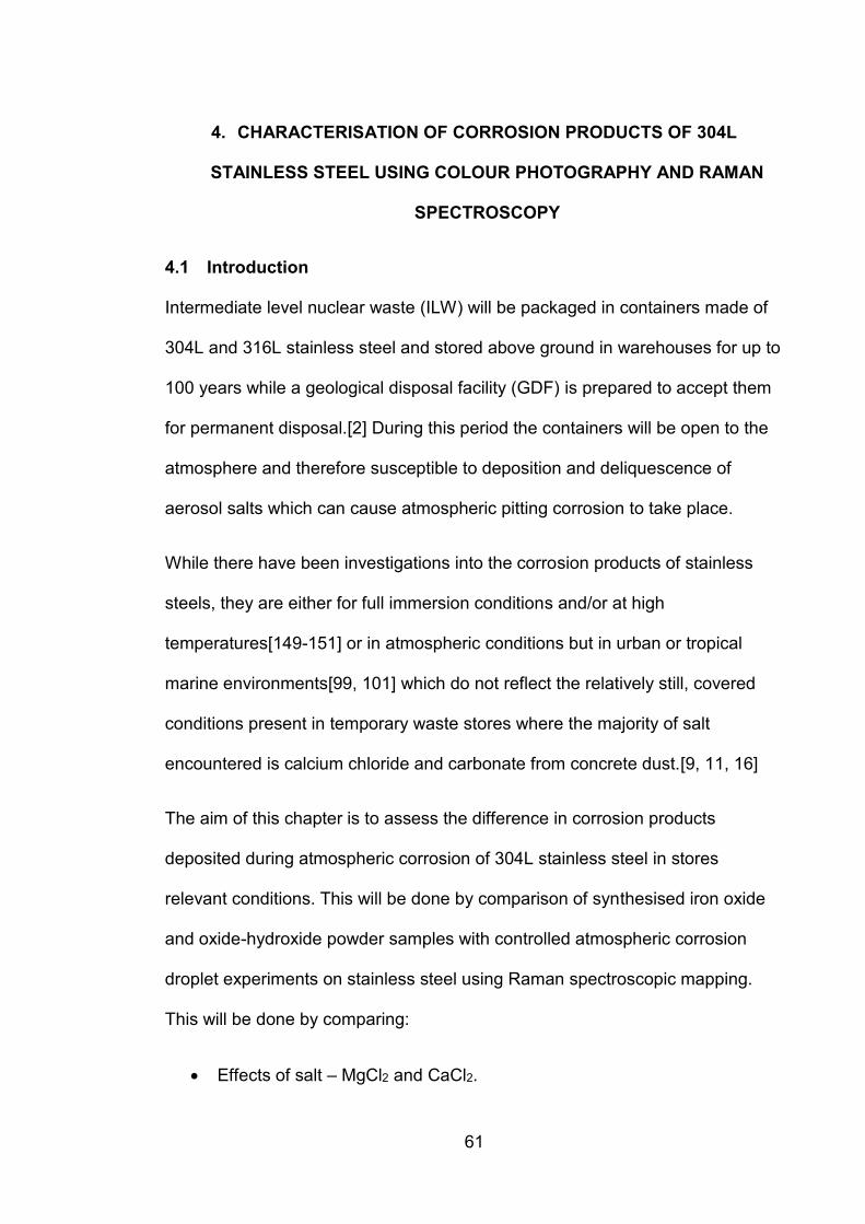
61

4. CHARACTERISATION OF CORROSION PRODUCTS OF 304L

STAINLESS STEEL USING COLOUR PHOTOGRAPHY AND RAMAN

SPECTROSCOPY

4.1 Introduction

Intermediate level nuclear waste (ILW) will be packaged in containers made of

304L and 316L stainless steel and stored above ground in warehouses for up to

100 years while a geological disposal facility (GDF) is prepared to accept them

for permanent disposal.[2] During this period the containers will be open to the

atmosphere and therefore susceptible to deposition and deliquescence of

aerosol salts which can cause atmospheric pitting corrosion to take place.

While there have been investigations into the corrosion products of stainless

steels, they are either for full immersion conditions and/or at high

temperatures[149-151] or in atmospheric conditions but in urban or tropical

marine environments[99, 101] which do not reflect the relatively still, covered

conditions present in temporary waste stores where the majority of salt

encountered is calcium chloride and carbonate from concrete dust.[9, 11, 16]

The aim of this chapter is to assess the difference in corrosion products

deposited during atmospheric corrosion of 304L stainless steel in stores

relevant conditions. This will be done by comparison of synthesised iron oxide

and oxide-hydroxide powder samples with controlled atmospheric corrosion

droplet experiments on stainless steel using Raman spectroscopic mapping.

This will be done by comparing:

Effects of salt – MgCl2 and CaCl2.

62

Effects of atmospheric conditions – fixed 46% RH, 30°C and fluctuating

ambient temperature and humidity on 100 μgcm-2 droplets exposed for

14 days

Effects of chloride deposition density (CDD) – 100 μgcm-2, 50 μgcm-2 and

20 μgcm-2 on MgCl2 droplets exposed for 24 days

Effects of exposure time – 100 μgcm-2 MgCl2 droplets exposed to fixed

46% RH, 30°C for 14 days and 24 days.

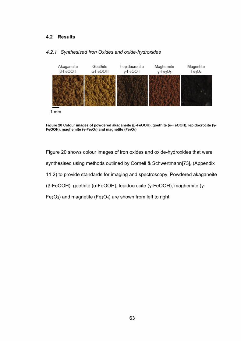
63

4.2 Results

4.2.1 Synthesised Iron Oxides and oxide-hydroxides

Figure 20 Colour images of powdered akaganeite (β-FeOOH), goethite (α-FeOOH), lepidocrocite (γ-FeOOH), maghemite (γ-Fe2O3) and magnetite (Fe3O4)

Figure 20 shows colour images of iron oxides and oxide-hydroxides that were

synthesised using methods outlined by Cornell & Schwertmann[73], (Appendix

11.2) to provide standards for imaging and spectroscopy. Powdered akaganeite

(β-FeOOH), goethite (α-FeOOH), lepidocrocite (γ-FeOOH), maghemite (γ-

Fe2O3) and magnetite (Fe3O4) are shown from left to right.

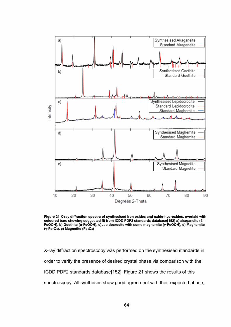
64

Figure 21 X-ray diffraction spectra of synthesised iron oxides and oxide-hydroxides, overlaid with coloured bars showing suggested fit from ICDD PDF2 standards database[152] a) akaganeite (β-FeOOH), b) Goethite (α-FeOOH), c)Lepidocrocite with some maghemite (γ-FeOOH), d) Maghemite (γ-Fe2O3), e) Magnetite (Fe3O4)

X-ray diffraction spectroscopy was performed on the synthesised standards in

order to verify the presence of desired crystal phase via comparison with the

ICDD PDF2 standards database[152]. Figure 21 shows the results of this

spectroscopy. All syntheses show good agreement with their expected phase,

65

apart from lepidocrocite which contains a significant fraction of maghemite. A

significant baseline is also present for lepidocrocite and to a lesser degree

akaganeite and magnetite.

66

Figure 22 Raman spectra of synthesised iron oxides and oxide-hydroxides a) akaganeite (β-FeOOH), b) Goethite (α-FeOOH), c) Lepidocrocite with some maghemite (γ-FeOOH), d) Maghemite (γ-Fe2O3), e) Magnetite (Fe3O4)

Raman spectroscopy was performed on the synthesised powders, shown in

Figure 22. a) Akaganeite has peaks at 300, 390, 520, 610 and 720 cm-1. b)

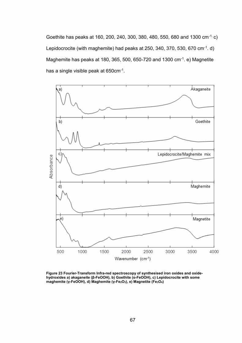
67

Goethite has peaks at 160, 200, 240, 300, 380, 480, 550, 680 and 1300 cm-1. c)

Lepidocrocite (with maghemite) had peaks at 250, 340, 370, 530, 670 cm-1. d)

Maghemite has peaks at 180, 365, 500, 650-720 and 1300 cm-1. e) Magnetite

has a single visible peak at 650cm-1.

Figure 23 Fourier-Transform Infra-red spectroscopy of synthesised iron oxides and oxide-hydroxides a) akaganeite (β-FeOOH), b) Goethite (α-FeOOH), c) Lepidocrocite with some maghemite (γ-FeOOH), d) Maghemite (γ-Fe2O3), e) Magnetite (Fe3O4)

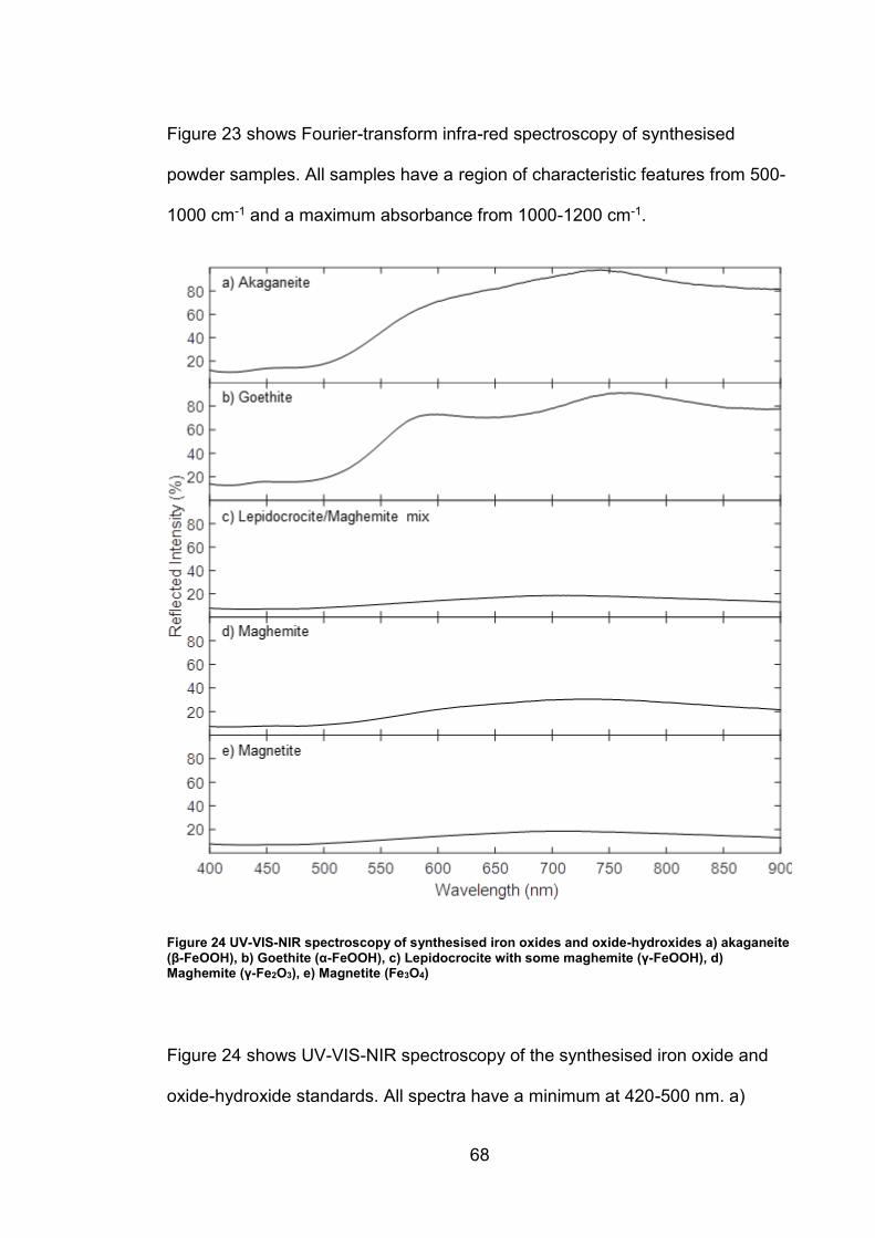
68

Figure 23 shows Fourier-transform infra-red spectroscopy of synthesised

powder samples. All samples have a region of characteristic features from 500-

1000 cm-1 and a maximum absorbance from 1000-1200 cm-1.

Figure 24 UV-VIS-NIR spectroscopy of synthesised iron oxides and oxide-hydroxides a) akaganeite (β-FeOOH), b) Goethite (α-FeOOH), c) Lepidocrocite with some maghemite (γ-FeOOH), d) Maghemite (γ-Fe2O3), e) Magnetite (Fe3O4)

Figure 24 shows UV-VIS-NIR spectroscopy of the synthesised iron oxide and

oxide-hydroxide standards. All spectra have a minimum at 420-500 nm. a)

69

Akaganeite (β-FeOOH) and b) Goethite (α-FeOOH) both show similar double

peaks at 575 and 775 nm and have the highest overall reflectance with a

maximum at 850 nm. The c) Lepidocrocite (γ-FeOOH)-maghemite mix, d)

Maghemite (γ-Fe2O3), e) Magnetite (Fe3O4) all reflect a much less light and

have a maximum reflectance at 700-750 nm of 20-30%.

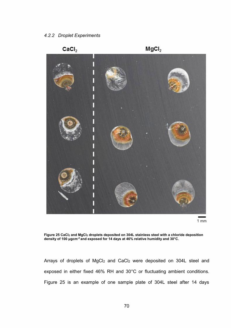
70

4.2.2 Droplet Experiments

Figure 25 CaCl2 and MgCl2 droplets deposited on 304L stainless steel with a chloride deposition density of 100 μgcm-2 and exposed for 14 days at 46% relative humidity and 30°C.

Arrays of droplets of MgCl2 and CaCl2 were deposited on 304L steel and

exposed in either fixed 46% RH and 30°C or fluctuating ambient conditions.

Figure 25 is an example of one sample plate of 304L steel after 14 days

71

exposed to fixed 46% RH and 30°C with CaCl2 and MgCl2 droplets of chloride

deposition density 100μgcm-2. All droplets contain pits. MgCl2 droplets exposed

to fixed conditions all have a dark ring of corrosion product directly around the

pit mouth, surrounded by a lighter ring of red-brown rust. This in turn is

surrounded by a white precipitate which occupies the rest of the droplet to the

edge. CaCl2 droplets exposed to fixed conditions similarly have a dark ring

directly around the pit surrounded by lighter red-brown rust. There is an

additional thick band of white precipitate immediately at the edge of the red-

brown rust and further small areas of white precipitate throughout the remainder

of the droplet. CaCl2 droplets that were exposed to fluctuating ambient

conditions have a similar red-brown ring of corrosion product surrounded by

white precipitated salt as the MgCl2 droplets exposed to fixed conditions. The

major difference is in a deep red corrosion product which has precipitated

directly over the pit mouth. MgCl2 droplet exposed to fluctuating conditions had

a thinner band of corrosion product and no precipitate. After 14 days a single,

representative droplet for each salt species and exposure condition was

selected for Raman mapping by similarity to other members of its set and

consistency of features. No sample preparation such as rinsing of salt solution

or corrosion product off the sample surface was performed for any photography

or Raman spectroscopy in this chapter. Measurements did not take place under

RH or temperature control, however, due to equipment limitations.

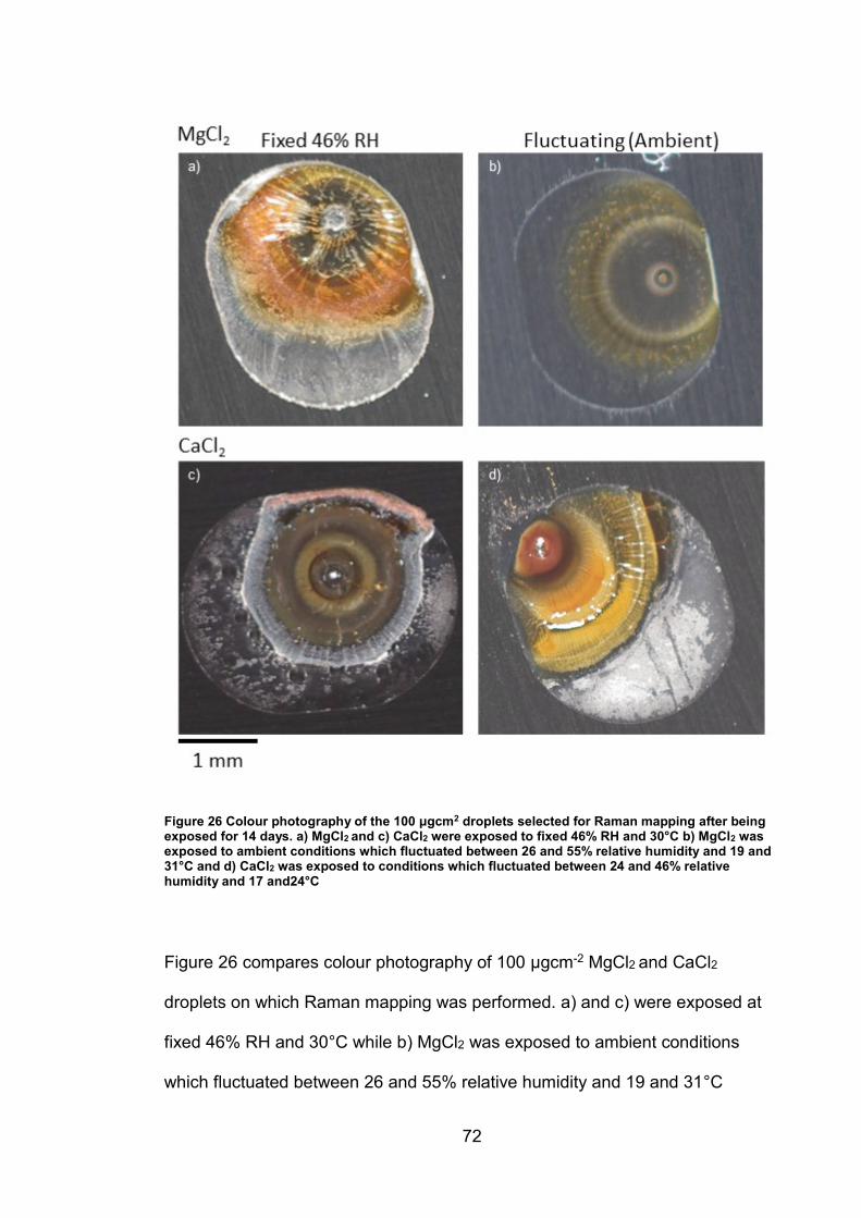
72

Figure 26 Colour photography of the 100 μgcm2 droplets selected for Raman mapping after being exposed for 14 days. a) MgCl2 and c) CaCl2 were exposed to fixed 46% RH and 30°C b) MgCl2 was exposed to ambient conditions which fluctuated between 26 and 55% relative humidity and 19 and 31°C and d) CaCl2 was exposed to conditions which fluctuated between 24 and 46% relative humidity and 17 and24°C

Figure 26 compares colour photography of 100 μgcm-2 MgCl2 and CaCl2

droplets on which Raman mapping was performed. a) and c) were exposed at

fixed 46% RH and 30°C while b) MgCl2 was exposed to ambient conditions

which fluctuated between 26 and 55% relative humidity and 19 and 31°C

73

(shown in detail in Figure 35) and d) CaCl2 was exposed to conditions which

fluctuated between 24 and 46% relative humidity and 17 and 27°C (Shown in

detail in Figure 36) a), b) and c) precipitated rust in a ring around the pit mouth,

which remains clear of corrosion product itself. d) had deeper, red rust directly

over the pit mouth. All droplets then had a region of white precipitate outside the

main rust region. This precipitate was dense immediately around the rust on

droplet c) while other droplets it was either evenly spread across the non-rusty

regions of the droplet or at denser the droplet edge.

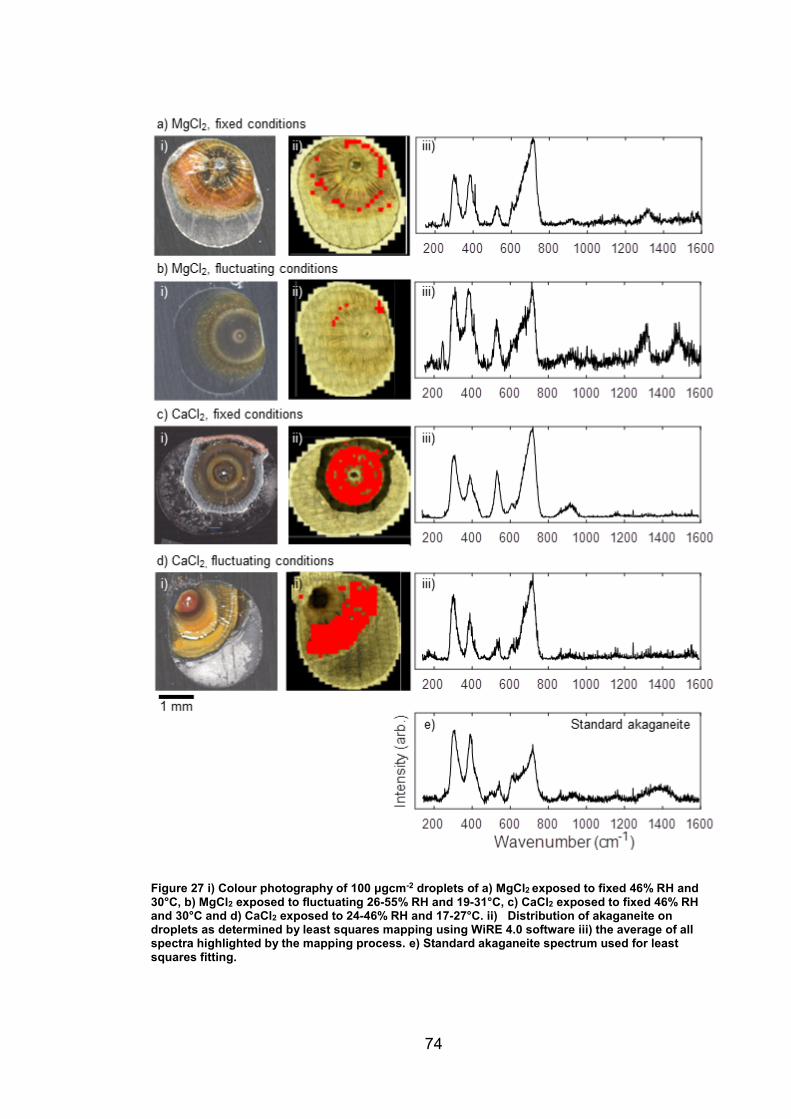
74

Figure 27 i) Colour photography of 100 μgcm-2 droplets of a) MgCl2 exposed to fixed 46% RH and 30°C, b) MgCl2 exposed to fluctuating 26-55% RH and 19-31°C, c) CaCl2 exposed to fixed 46% RH and 30°C and d) CaCl2 exposed to 24-46% RH and 17-27°C. ii) Distribution of akaganeite on droplets as determined by least squares mapping using WiRE 4.0 software iii) the average of all spectra highlighted by the mapping process. e) Standard akaganeite spectrum used for least squares fitting.

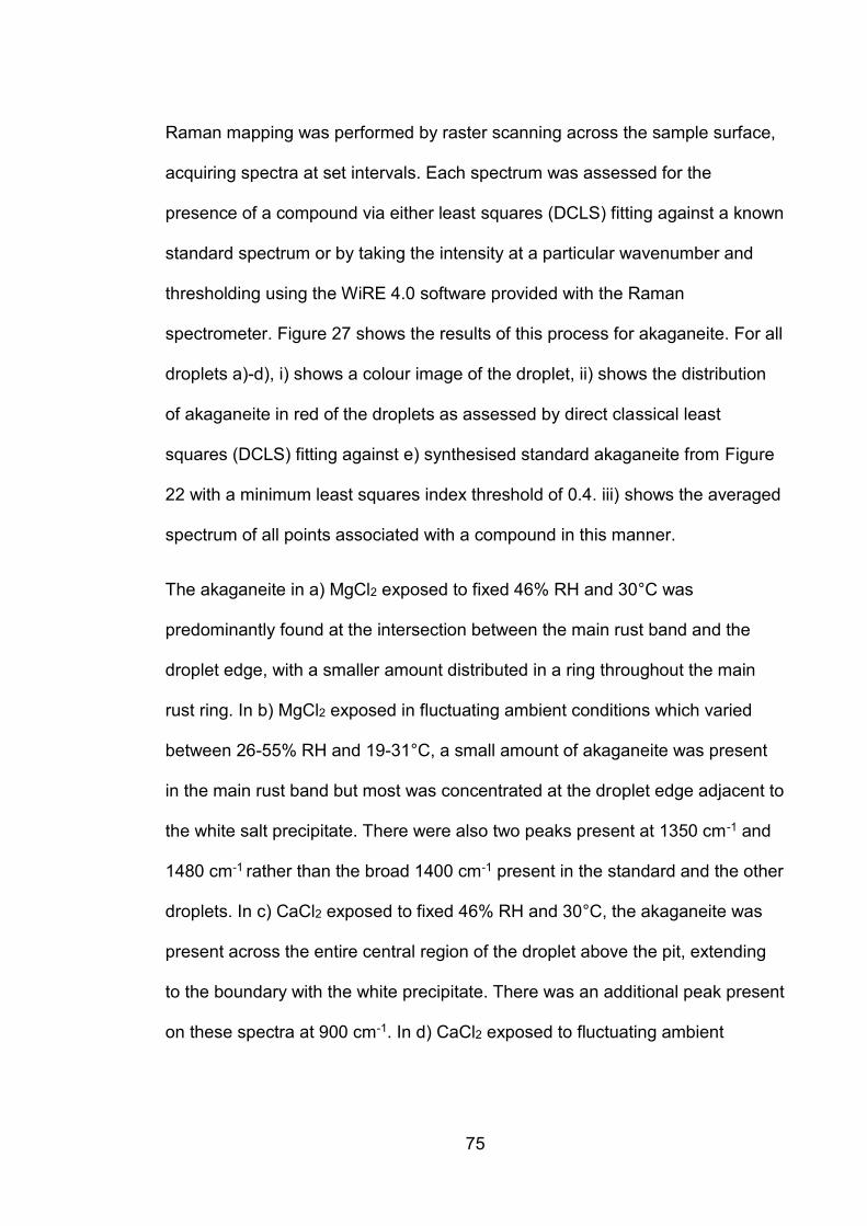
75

Raman mapping was performed by raster scanning across the sample surface,

acquiring spectra at set intervals. Each spectrum was assessed for the

presence of a compound via either least squares (DCLS) fitting against a known

standard spectrum or by taking the intensity at a particular wavenumber and

thresholding using the WiRE 4.0 software provided with the Raman

spectrometer. Figure 27 shows the results of this process for akaganeite. For all

droplets a)-d), i) shows a colour image of the droplet, ii) shows the distribution

of akaganeite in red of the droplets as assessed by direct classical least

squares (DCLS) fitting against e) synthesised standard akaganeite from Figure

22 with a minimum least squares index threshold of 0.4. iii) shows the averaged

spectrum of all points associated with a compound in this manner.

The akaganeite in a) MgCl2 exposed to fixed 46% RH and 30°C was

predominantly found at the intersection between the main rust band and the

droplet edge, with a smaller amount distributed in a ring throughout the main

rust ring. In b) MgCl2 exposed in fluctuating ambient conditions which varied

between 26-55% RH and 19-31°C, a small amount of akaganeite was present

in the main rust band but most was concentrated at the droplet edge adjacent to

the white salt precipitate. There were also two peaks present at 1350 cm-1 and

1480 cm-1 rather than the broad 1400 cm-1 present in the standard and the other

droplets. In c) CaCl2 exposed to fixed 46% RH and 30°C, the akaganeite was

present across the entire central region of the droplet above the pit, extending

to the boundary with the white precipitate. There was an additional peak present

on these spectra at 900 cm-1. In d) CaCl2 exposed to fluctuating ambient

76

conditions which varied between 24-46% RH and 17-27°C the akaganeite was

concentrated in a band across the droplet away from the pit mouth.

Figure 28 i) Colour photography of 100 μgcm-2 droplets of a) MgCl2 exposed to fixed 46% RH and 30°C, b) MgCl2 exposed to fluctuating 26-55% RH and 19-31°C. ii) Distribution of lepidocrocite on droplets as determined by least squares mapping using WiRE 4.0 software iii) the average of all spectra highlighted by the mapping process. c) Standard lepidocrocite taken from a weathering steel sample spectrum used for least squares fitting along with the spectrum from the synthesised lepidocrocite.

Figure 28 shows the distribution of lepidocrocite as determined by least squares

fitting of a lepidocrocite spectrum taken from a weathering steel sample (chosen

for similarity to literature spectra[81-83]). a,b) i) shows a colour image of the

droplet, ii) shows the distribution of akaganeite in red of the droplets as

assessed by direct classical least squares (DCLS) fitting with a minimum least

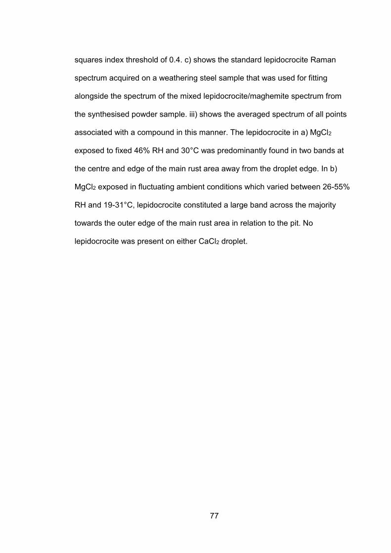
77

squares index threshold of 0.4. c) shows the standard lepidocrocite Raman

spectrum acquired on a weathering steel sample that was used for fitting

alongside the spectrum of the mixed lepidocrocite/maghemite spectrum from

the synthesised powder sample. iii) shows the averaged spectrum of all points

associated with a compound in this manner. The lepidocrocite in a) MgCl2

exposed to fixed 46% RH and 30°C was predominantly found in two bands at

the centre and edge of the main rust area away from the droplet edge. In b)

MgCl2 exposed in fluctuating ambient conditions which varied between 26-55%

RH and 19-31°C, lepidocrocite constituted a large band across the majority

towards the outer edge of the main rust area in relation to the pit. No

lepidocrocite was present on either CaCl2 droplet.

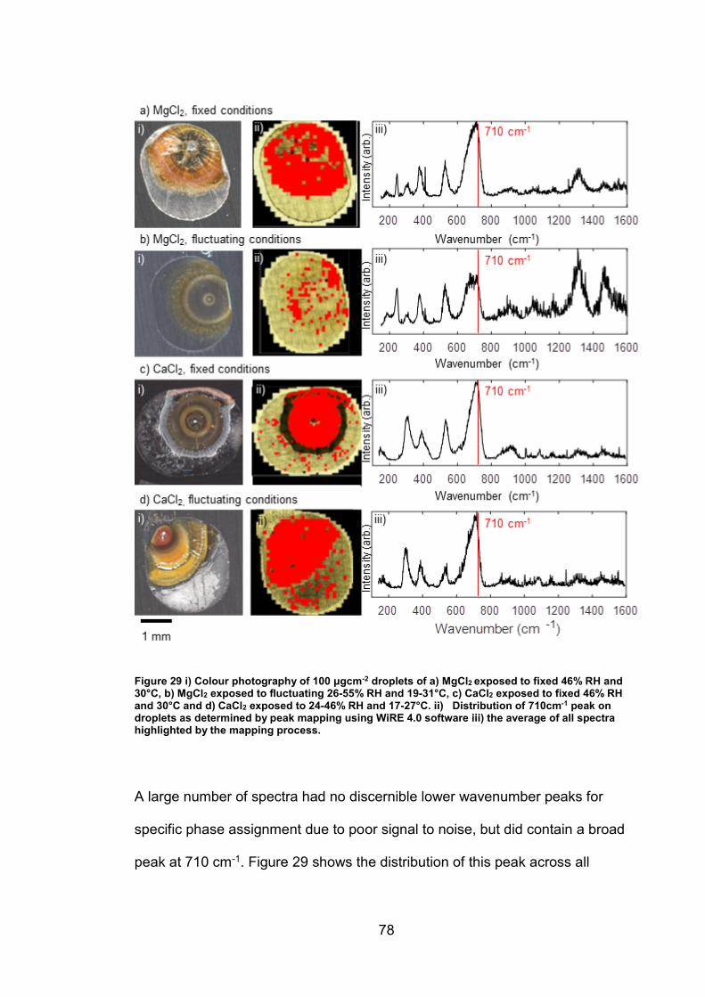
78

Figure 29 i) Colour photography of 100 μgcm-2 droplets of a) MgCl2 exposed to fixed 46% RH and 30°C, b) MgCl2 exposed to fluctuating 26-55% RH and 19-31°C, c) CaCl2 exposed to fixed 46% RH and 30°C and d) CaCl2 exposed to 24-46% RH and 17-27°C. ii) Distribution of 710cm-1 peak on droplets as determined by peak mapping using WiRE 4.0 software iii) the average of all spectra highlighted by the mapping process.

A large number of spectra had no discernible lower wavenumber peaks for

specific phase assignment due to poor signal to noise, but did contain a broad

peak at 710 cm-1. Figure 29 shows the distribution of this peak across all

79

droplets a-d). i) shows colour photographs of the droplet, a-d) ii) shows maps

created by highlighting all spectra with an intensity about 150 at a wavenumber

710 cm-1 a-d) iii) are the average spectrum of all highlighted pixels in an

associated droplet.

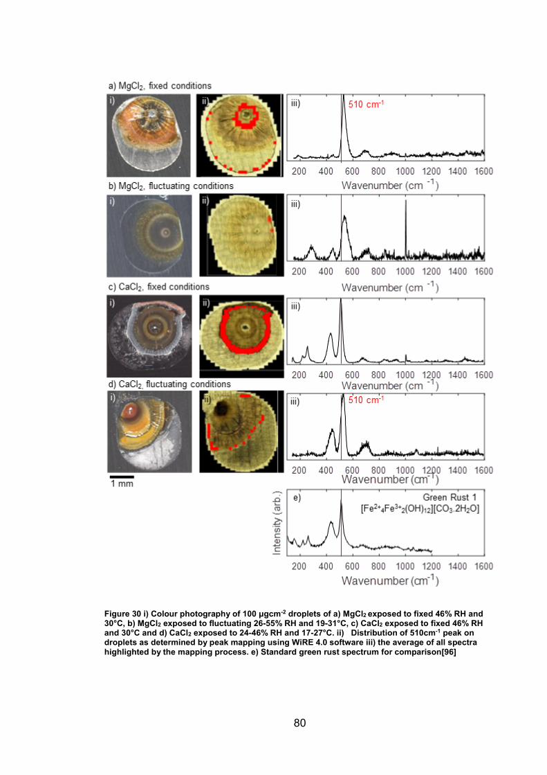
80

Figure 30 i) Colour photography of 100 μgcm-2 droplets of a) MgCl2 exposed to fixed 46% RH and 30°C, b) MgCl2 exposed to fluctuating 26-55% RH and 19-31°C, c) CaCl2 exposed to fixed 46% RH and 30°C and d) CaCl2 exposed to 24-46% RH and 17-27°C. ii) Distribution of 510cm-1 peak on droplets as determined by peak mapping using WiRE 4.0 software iii) the average of all spectra highlighted by the mapping process. e) Standard green rust spectrum for comparison[96]

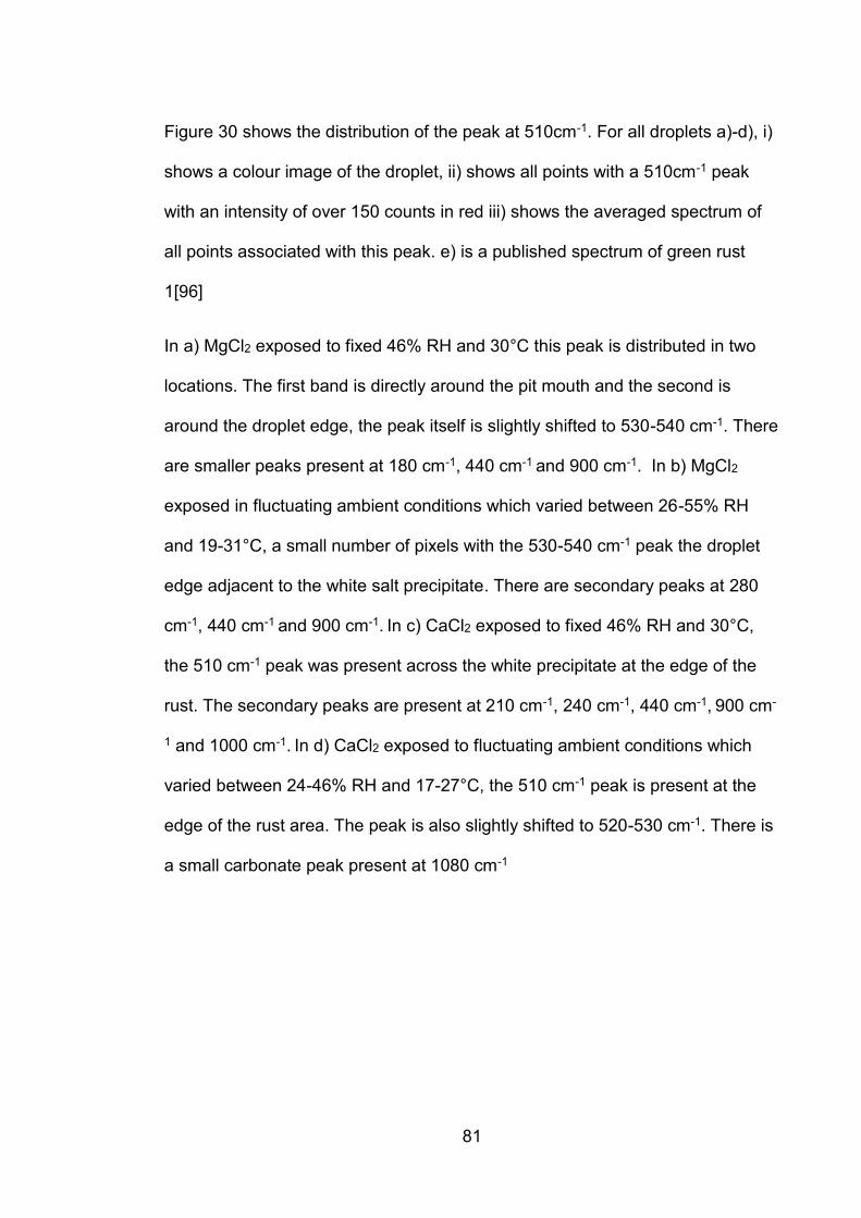
81

Figure 30 shows the distribution of the peak at 510cm-1. For all droplets a)-d), i)

shows a colour image of the droplet, ii) shows all points with a 510cm-1 peak

with an intensity of over 150 counts in red iii) shows the averaged spectrum of

all points associated with this peak. e) is a published spectrum of green rust

1[96]

In a) MgCl2 exposed to fixed 46% RH and 30°C this peak is distributed in two

locations. The first band is directly around the pit mouth and the second is

around the droplet edge, the peak itself is slightly shifted to 530-540 cm-1. There

are smaller peaks present at 180 cm-1, 440 cm-1 and 900 cm-1. In b) MgCl2

exposed in fluctuating ambient conditions which varied between 26-55% RH

and 19-31°C, a small number of pixels with the 530-540 cm-1 peak the droplet

edge adjacent to the white salt precipitate. There are secondary peaks at 280

cm-1, 440 cm-1 and 900 cm-1. In c) CaCl2 exposed to fixed 46% RH and 30°C,

the 510 cm-1 peak was present across the white precipitate at the edge of the

rust. The secondary peaks are present at 210 cm-1, 240 cm-1, 440 cm-1, 900 cm-

1 and 1000 cm-1. In d) CaCl2 exposed to fluctuating ambient conditions which

varied between 24-46% RH and 17-27°C, the 510 cm-1 peak is present at the

edge of the rust area. The peak is also slightly shifted to 520-530 cm-1. There is

a small carbonate peak present at 1080 cm-1

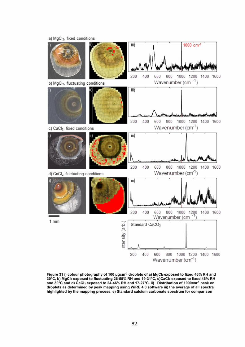
82

Figure 31 i) colour photography of 100 μgcm-2 droplets of a) MgCl2 exposed to fixed 46% RH and 30°C, b) MgCl2 exposed to fluctuating 26-55% RH and 19-31°C, c)CaCl2 exposed to fixed 46% RH and 30°C and d) CaCl2 exposed to 24-46% RH and 17-27°C. ii) Distribution of 1000cm-1 peak on droplets as determined by peak mapping using WiRE 4.0 software iii) the average of all spectra highlighted by the mapping process. e) Standard calcium carbonate spectrum for comparison

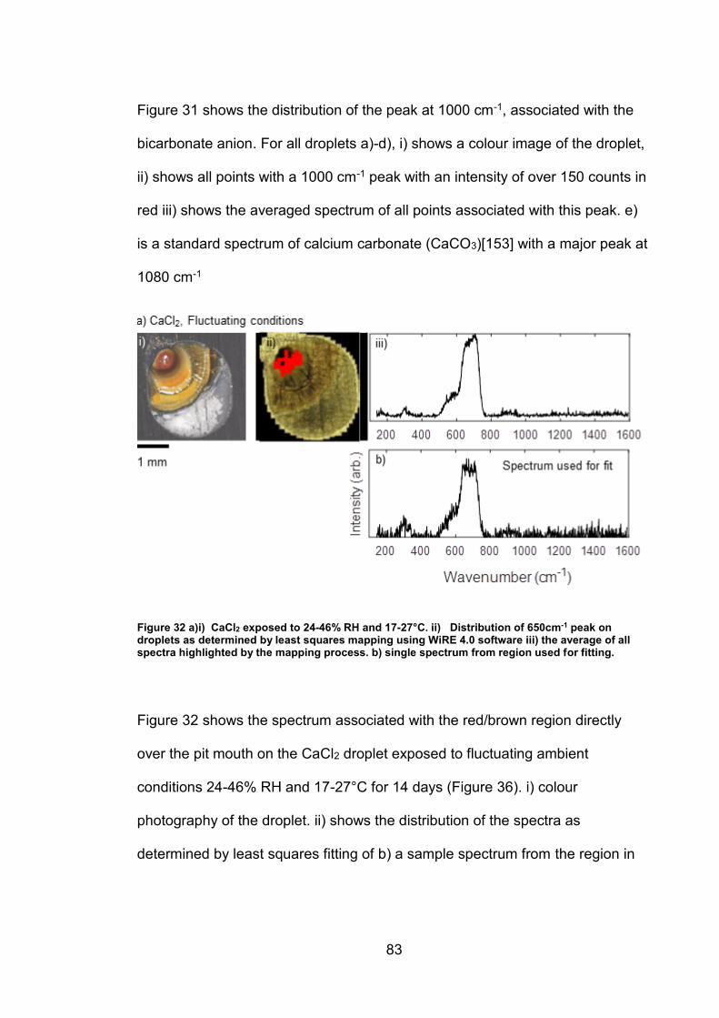
83

Figure 31 shows the distribution of the peak at 1000 cm-1, associated with the

bicarbonate anion. For all droplets a)-d), i) shows a colour image of the droplet,

ii) shows all points with a 1000 cm-1 peak with an intensity of over 150 counts in

red iii) shows the averaged spectrum of all points associated with this peak. e)

is a standard spectrum of calcium carbonate (CaCO3)[153] with a major peak at

1080 cm-1

Figure 32 a)i) CaCl2 exposed to 24-46% RH and 17-27°C. ii) Distribution of 650cm-1 peak on droplets as determined by least squares mapping using WiRE 4.0 software iii) the average of all spectra highlighted by the mapping process. b) single spectrum from region used for fitting.

Figure 32 shows the spectrum associated with the red/brown region directly

over the pit mouth on the CaCl2 droplet exposed to fluctuating ambient

conditions 24-46% RH and 17-27°C for 14 days (Figure 36). i) colour

photography of the droplet. ii) shows the distribution of the spectra as

determined by least squares fitting of b) a sample spectrum from the region in

84

question. iii) shows the average of the 30 spectra associated with the region by

least squares fitting with a threshold of 0.8 least squares index.

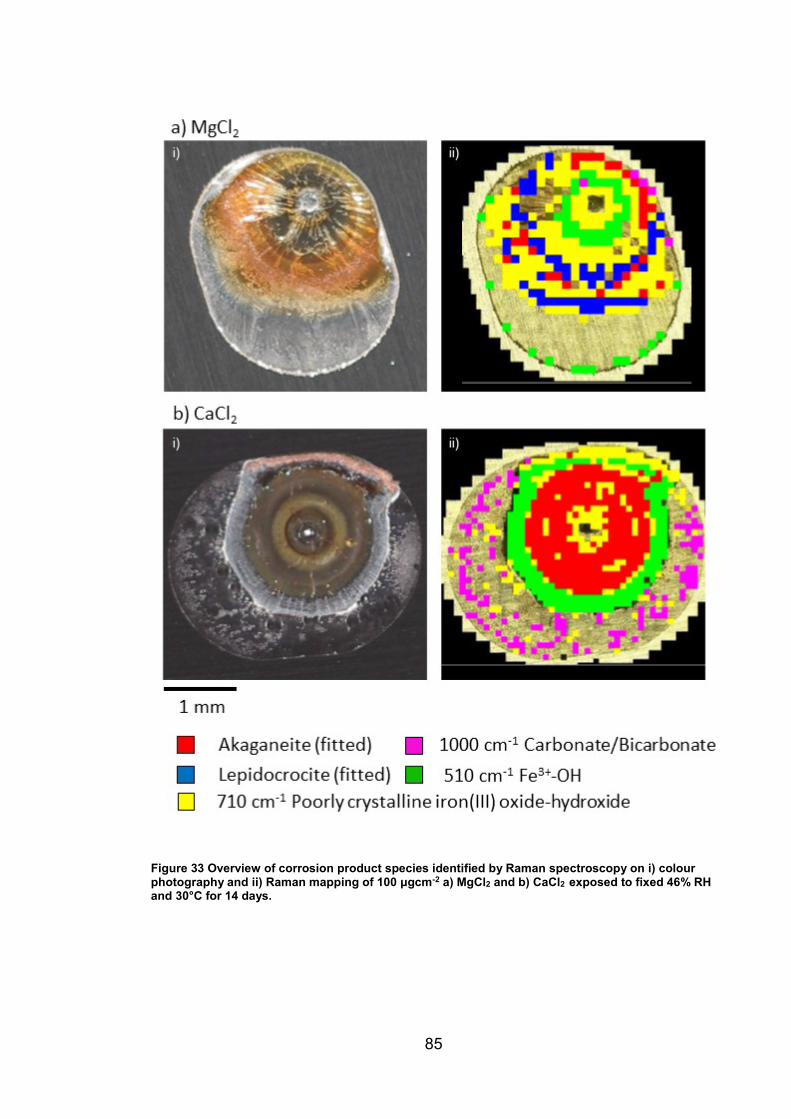
85

Figure 33 Overview of corrosion product species identified by Raman spectroscopy on i) colour photography and ii) Raman mapping of 100 μgcm-2 a) MgCl2 and b) CaCl2 exposed to fixed 46% RH and 30°C for 14 days.

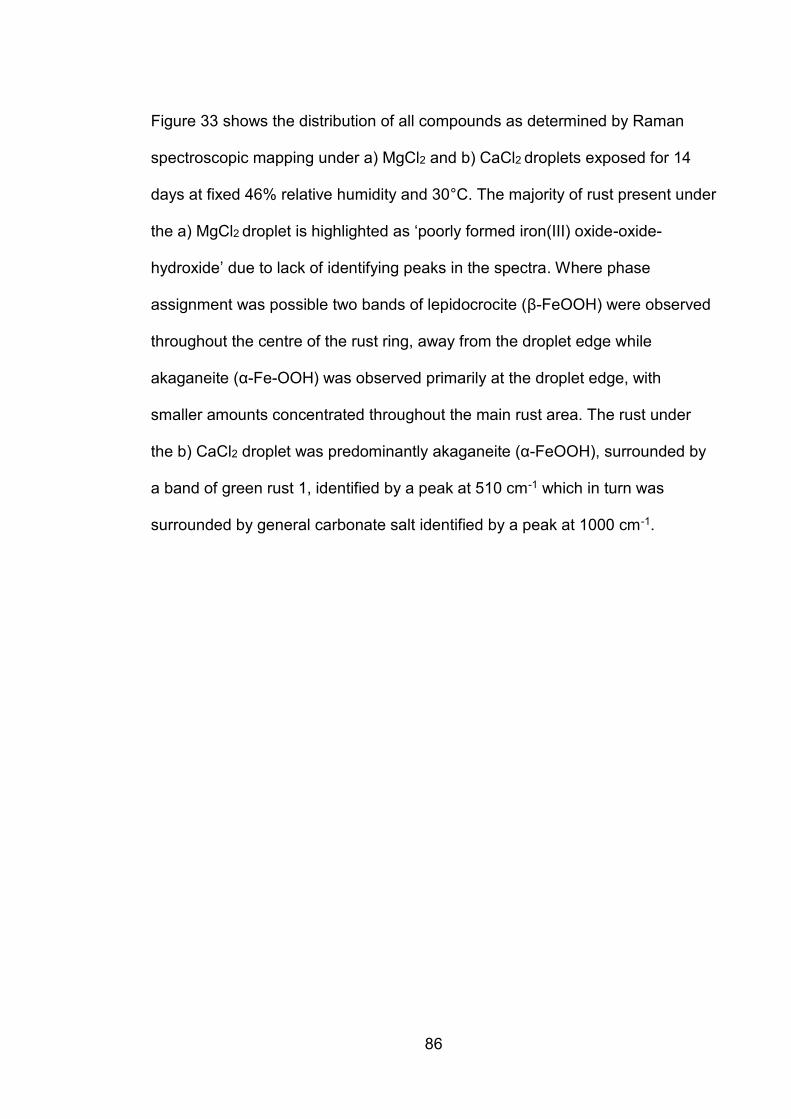
86

Figure 33 shows the distribution of all compounds as determined by Raman

spectroscopic mapping under a) MgCl2 and b) CaCl2 droplets exposed for 14

days at fixed 46% relative humidity and 30°C. The majority of rust present under

the a) MgCl2 droplet is highlighted as ‘poorly formed iron(III) oxide-oxide-

hydroxide’ due to lack of identifying peaks in the spectra. Where phase

assignment was possible two bands of lepidocrocite (β-FeOOH) were observed

throughout the centre of the rust ring, away from the droplet edge while

akaganeite (α-Fe-OOH) was observed primarily at the droplet edge, with

smaller amounts concentrated throughout the main rust area. The rust under

the b) CaCl2 droplet was predominantly akaganeite (α-FeOOH), surrounded by

a band of green rust 1, identified by a peak at 510 cm-1 which in turn was

surrounded by general carbonate salt identified by a peak at 1000 cm-1.

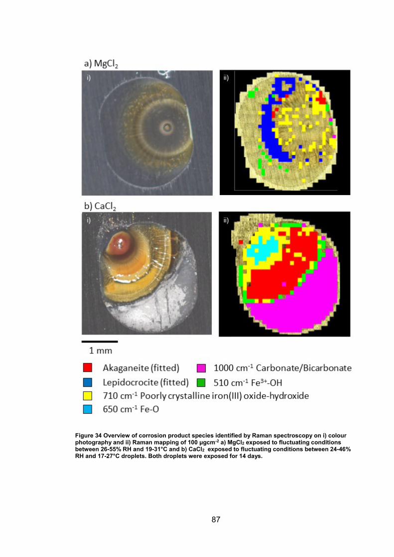
87

Figure 34 Overview of corrosion product species identified by Raman spectroscopy on i) colour photography and ii) Raman mapping of 100 μgcm-2 a) MgCl2 exposed to fluctuating conditions between 26-55% RH and 19-31°C and b) CaCl2 exposed to fluctuating conditions between 24-46% RH and 17-27°C droplets. Both droplets were exposed for 14 days.

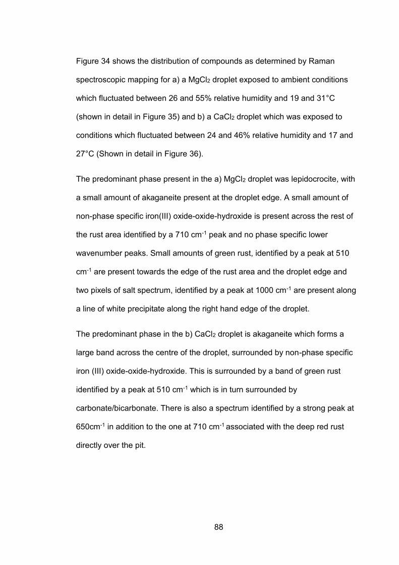
88

Figure 34 shows the distribution of compounds as determined by Raman

spectroscopic mapping for a) a MgCl2 droplet exposed to ambient conditions

which fluctuated between 26 and 55% relative humidity and 19 and 31°C

(shown in detail in Figure 35) and b) a CaCl2 droplet which was exposed to

conditions which fluctuated between 24 and 46% relative humidity and 17 and

27°C (Shown in detail in Figure 36).

The predominant phase present in the a) MgCl2 droplet was lepidocrocite, with

a small amount of akaganeite present at the droplet edge. A small amount of

non-phase specific iron(III) oxide-oxide-hydroxide is present across the rest of

the rust area identified by a 710 cm-1 peak and no phase specific lower

wavenumber peaks. Small amounts of green rust, identified by a peak at 510

cm-1 are present towards the edge of the rust area and the droplet edge and

two pixels of salt spectrum, identified by a peak at 1000 cm-1 are present along

a line of white precipitate along the right hand edge of the droplet.

The predominant phase in the b) CaCl2 droplet is akaganeite which forms a

large band across the centre of the droplet, surrounded by non-phase specific

iron (III) oxide-oxide-hydroxide. This is surrounded by a band of green rust

identified by a peak at 510 cm-1 which is in turn surrounded by

carbonate/bicarbonate. There is also a spectrum identified by a strong peak at

650cm-1 in addition to the one at 710 cm-1 associated with the deep red rust

directly over the pit.

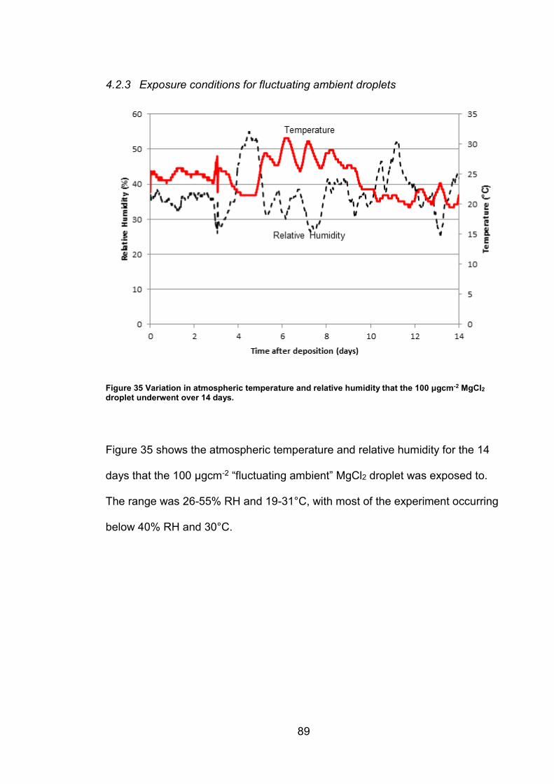
89

4.2.3 Exposure conditions for fluctuating ambient droplets

Figure 35 Variation in atmospheric temperature and relative humidity that the 100 μgcm-2 MgCl2

droplet underwent over 14 days.

Figure 35 shows the atmospheric temperature and relative humidity for the 14

days that the 100 μgcm-2 “fluctuating ambient” MgCl2 droplet was exposed to.

The range was 26-55% RH and 19-31°C, with most of the experiment occurring

below 40% RH and 30°C.

90

Figure 36 Variation in atmospheric temperature and relative humidity that the 100 μgcm-2 CaCl2

droplet underwent over 14 days. .

Figure 36 shows the atmospheric temperature and relative humidity for the 14

days that the 100 μgcm-2 “fluctuating ambient” MgCl2 droplet was exposed to.

The range was 24-46% RH and 17-24°C with most of the experiment occurring

below 40% RH and 25°C.

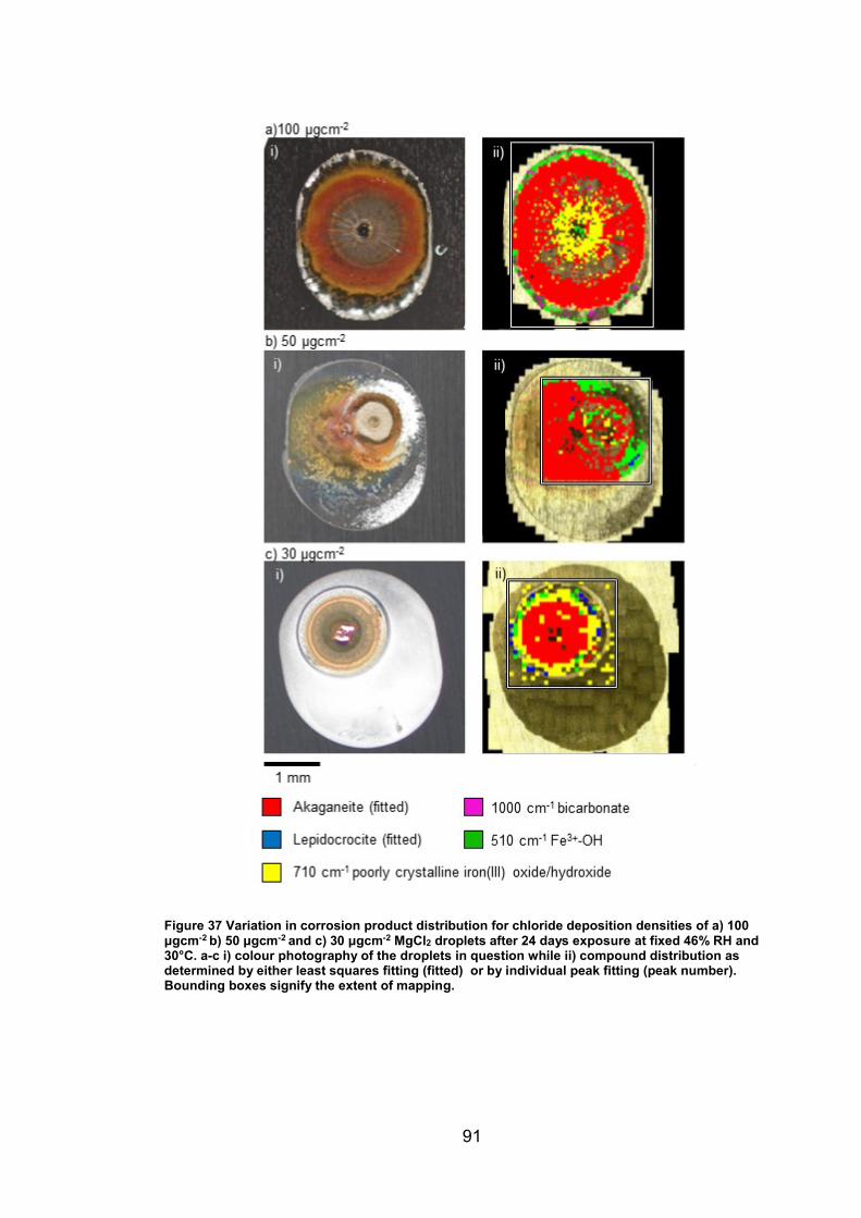
91

Figure 37 Variation in corrosion product distribution for chloride deposition densities of a) 100 μgcm-2 b) 50 μgcm-2 and c) 30 μgcm-2 MgCl2 droplets after 24 days exposure at fixed 46% RH and 30°C. a-c i) colour photography of the droplets in question while ii) compound distribution as determined by either least squares fitting (fitted) or by individual peak fitting (peak number). Bounding boxes signify the extent of mapping.

92

Figure 37 shows the distribution of corrosion products as determined by Raman

spectroscopic mapping under a) 100 μgcm-2, b) 50 μgcm-2 and c) 30 μgcm-2

MgCl2 droplets exposed for 14 days at fixed 46% relative humidity and 30°C.

Raman spectra were taken at intervals across the sample surface and analysed

to determine the presence of a particular compound. Akaganeite and

lepidocrocite presence was determined by ‘direct classical least squares’

(DCLS) fitting experimentally acquired spectra against synthesised standards

using WiRE 4.0. Carbonate, green rust and poorly crystalline iron(III) oxide-

oxide-hydroxide were determined by mapping the presence of a single

characteristic peak. These were at 1000 cm-1 for carbonate/bicarbonate, 510cm-

1 for green rust and 710 cm-1 for poorly crystalline iron(III) oxide-oxide-

hydroxide. Minimum thresholds for assigning a compound to a pixel were 0.4 for

the DCLS method or an intensity of 150 counts for the peak presence method.

The predominant phase of iron oxide-hydroxide on all droplets in Figure 37 is

akaganeite, with minor regions consisting of lepidocrocite only present on the b)

50 μgcm-2 and c) 30 μgcm-2 droplets along the outer edge of the rust area. All

pixels with the presence of an iron oxide-hydroxide specific peak at 710 cm-1

but no minor phase specific peaks at lower wavenumbers were assigned as

poorly formed iron(III) oxide-oxide-hydroxide. Outside the iron oxide-hydroxide

region, spectra with a strong peak at 510 cm-1 associated with Fe3+-OH are

present. Bicarbonate, identified by a peak at 1000cm-1 was only observed on

the a) 100 μgcm-2 droplet.

93

4.3 Discussion

The distribution of corrosion products of 304L stainless steel was assessed by

Raman spectroscopy for multiple chloride deposition densities (CDDs) of MgCl2

and CaCl2 droplets exposed for 14 and 24 days in both fixed and fluctuating

ambient conditions. Iron oxide-hydroxide phase assignment was performed by

direct classical least squares (DCLS) fitting against synthesised iron oxide-

hydroxide standards, remaining compounds were identified by fitting of

individual characteristic peaks and comparing them to spectra found in

literature.

4.3.1 Identification and assignment of compounds

Iron(III) oxide-hydroxides, identified by a broad peak from 650-710 cm-1

constituted the majority of corrosion product identified. Significant numbers of

spectra had poor signal to noise and no discernable peaks at lower

wavenumber characteristic which would identify it as a specific phase, and so

fitting was performed by presence of the main peak at 710 cm-1 for these

regions (Figure 29). This lack of identifying spectral features is associated with

poor crystallinity[81, 82] and as such these points likely have a highly hydrated

mix of ferrihydrite (2-line and 6 line) [77] which have a similar broad peak at

360-400 cm-1 and 710 cm-1. This is supported by the higher incidence of more

regular crystalline akaganeite on the MgCl2 exposed to fixed conditions for 24

days (Figure 37) when compared to the one exposed for 14 days (Figure 33).

Akaganeite and lepidocrocite were the only specific iron oxide-hydroxide

phases identified. Their presence was determined by least squares fitting

against synthesized iron oxide-hydroxide powders (Figure 20) which had purity

94

verified by XRD spectroscopy (Figure 21). Due to the maghemite present in the

lepidocrocite standard, a lepidocrocite spectrum from weathering steel was

used which better agreed with lepidocrocite spectra present in the literature [76-

83, 91, 92, 96, 99-101, 149, 151, 154-158]

The formation of akaganeite is known to be favoured in the acidic, high chloride

concentration environments[73] which are present under droplets during

atmospheric corrosion. Without such a high chloride concentration environment,

it’s likely that goethite would form instead. The formation of lepidocrocite is also

pH dependent, but occurs in less acidic conditions (pH5-7) and is known to form

via a green rust intermediary as well as by direct precipitation from Fe3+

species[73] suggesting that former green rust regions could be tracked via

lepidocrocite presence.

“Green rusts” (Figure 30) were identified by their large 510 cm-1 peak which is

attributed to the Fe3+-OH stretching mode.[159] Legrand demonstrated that the

ratio of 450 cm-1 (Fe2+-OH) peak area to that of the 510 cm-1 (Fe3+-OH) peak

allows us to infer chemistry of the green rust.[96] As such, the reduced peak

ratios in MgCl2 droplets suggest that we might instead be looking at a similar

double layered hydroxide (LDH) of the hydrotalcite supergroup such as

Coalingite (Mg10Fe3+2(CO3)(OH)24·2H2O) or Iowaite (Mg6Fe3+

2(OH)16Cl2·4H2O)

for MgCl2 droplets. The spectrum present on CaCl2 droplets agrees with the one

described by Legrand, with additional peaks at 280 cm-1, 1000 cm-1 and 1080

cm-1.

95

Many spectra present a peak at 900 cm-1 which was attributed to

perchlorate.[160, 161] Bicarbonate peaks were also present on all droplets at

1000 cm-1, CaCl2 droplets also had carbonate peaks at 1080 cm-1.[160]

4.3.2 Distribution of compounds by cation

A broad peak at 710 cm-1 indicating iron(III) oxide-hydroxide was present across

all red-brown rusty regions on all droplets (Figure 29), in many places this peak

was present without additional peaks that would denote a particular crystal

phase such as lepidocrocite (Figure 28) or akaganeite (Figure 27). Where better

crystallinity is observed i.e. the spectrum has a greater signal to noise ratio and

peaks are more easily discernable, akaganeite favours CaCl2 droplets while

lepidocrocite favours MgCl2 and is not present on CaCl2 droplets. It is known that

a major pathway for the formation of lepidocrocite is via a green rust

intermediary[73] and as such the lack of lepidocrocite on CaCl2 droplets could

be due to a longer lived GR species which does not transform to lepidocrocite

as readily. This is supported by the lack of a well matching GR spectrum with

peaks at 280 cm-1 and 450 cm-1 on the MgCl2 droplet exposed in fixed

conditions and that the distribution of lepidocrocite on this droplet occupies a

similar location to the green rust on the CaCl2 droplets, along the edge of the

rust area.

All droplets have a region outside the main rust area where a white substance

precipitates. On MgCl2 droplets this was found to be solely bicarbonate, while in

CaCl2 it was a mix of carbonate and bicarbonate.

96

4.3.3 Distribution of compounds over time

Two 100 μgcm-2 MgCl2 droplets exposed to fixed conditions were analysed, one

after 14 days exposure(Figure 33), the other after 24 days (Figure 37). The

proportion of well crystallised iron oxide-hydroxide phases is much larger on the

24 day droplet compared to the 14 day as crystallinity improves over time. It’s

also worth noting that the 14 day droplet shows a mix of lepidocrocite and

akaganeite when a phase could be assigned while the 24 day droplet solely

presents akaganeite.

4.3.4 Distribution of compounds by chloride deposition density

Figure 37 shows 100 μgcm-2, 50 cm-2 and 20 μgcm-2 MgCl2 droplets that were

exposed for 24 days to fixed 46% RH and 30°C conditions before Raman

mapping was performed to assess how corrosion product distribution varied

with chloride deposition density. The distribution of species was similar across

all CDDs, with iron oxide-hydroxide deposited over and around the pit mouth,

surrounded by a band of Fe3+-OH indicating presence of green rust or green

rust-like layered double hydroxide. The predominant iron oxide-hydroxide phase

on all droplets was akaganeite, with only small amounts of lepidocrocite present

at the interface between the iron oxide-hydroxide rust area and points bearing

green rust. The green rust-like region was in turn surrounded by regions of

white precipitate which were likely bicarbonate, but fluoresced too heavily for

specific peaks to be identifiable. The main difference between CDDs was the

extent of the rust area, with a higher CDD having a larger extent of iron oxide-

hydroxide. This could be due to the electrolyte layer being thicker for higher

chloride deposition densities, meaning that more charge carriers are available

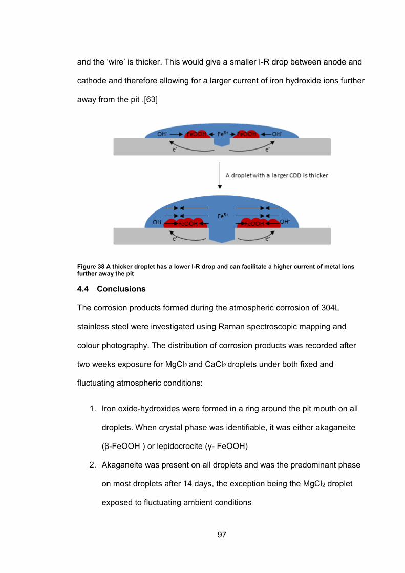
97

and the ‘wire’ is thicker. This would give a smaller I-R drop between anode and

cathode and therefore allowing for a larger current of iron hydroxide ions further

away from the pit .[63]

Figure 38 A thicker droplet has a lower I-R drop and can facilitate a higher current of metal ions further away the pit

4.4 Conclusions

The corrosion products formed during the atmospheric corrosion of 304L

stainless steel were investigated using Raman spectroscopic mapping and

colour photography. The distribution of corrosion products was recorded after

two weeks exposure for MgCl2 and CaCl2 droplets under both fixed and

fluctuating atmospheric conditions:

1. Iron oxide-hydroxides were formed in a ring around the pit mouth on all

droplets. When crystal phase was identifiable, it was either akaganeite

(β-FeOOH ) or lepidocrocite (γ- FeOOH)

2. Akaganeite was present on all droplets and was the predominant phase

on most droplets after 14 days, the exception being the MgCl2 droplet

exposed to fluctuating ambient conditions

98

3. Lepidocrocite was only observed on MgCl2 droplets and was the

predominant phase on the MgCl2 droplet exposed to ambient conditions

after 14 days.

4. Layered double iron oxide-hydroxides were formed on all droplets. On

CaCl2 this was green rust 1 (Carbonate, fougerite group) and was

present in a ring around the main iron oxide-hydroxide region. Specific

mineral allocation was difficult for similar spectra on MgCl2 droplets.

5. The white precipitate which surrounded the iron oxide-hydroxide was

comprised of carbonate and bicarbonate.

The distribution of corrosion products of 304L under different chloride

deposition densities was also investigated by Raman mapping of MgCl2

droplets after a 24 day exposure to fixed 46% RH and 30°C where a larger

region of iron oxide-hydroxide was associated with a higher chloride

deposition density. Additionally, when a 100 μgcm-2 MgCl2 droplet that was

exposed for 14 days in fixed conditions was compared with one exposed for

24 days, proportionally more of the iron oxide-hydroxide species was

akaganeite, indicating that crystallinity improves over time

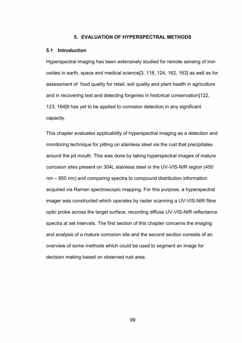
99

5. EVALUATION OF HYPERSPECTRAL METHODS

5.1 Introduction

Hyperspectral imaging has been extensively studied for remote sensing of iron

oxides in earth, space and medical science[3, 118, 124, 162, 163] as well as for

assessment of food quality for retail, soil quality and plant health in agriculture

and in recovering text and detecting forgeries in historical conservation[122,

123, 164]It has yet to be applied to corrosion detection in any significant

capacity.

This chapter evaluates applicability of hyperspectral imaging as a detection and

monitoring technique for pitting on stainless steel via the rust that precipitates

around the pit mouth. This was done by taking hyperspectral images of mature

corrosion sites present on 304L stainless steel in the UV-VIS-NIR region (450

nm – 850 nm) and comparing spectra to compound distribution information

acquired via Raman spectroscopic mapping. For this purpose, a hyperspectral

imager was constructed which operates by raster scanning a UV-VIS-NIR fibre

optic probe across the target surface, recording diffuse UV-VIS-NIR reflectance

spectra at set intervals. The first section of this chapter concerns the imaging

and analysis of a mature corrosion site and the second section consists of an

overview of some methods which could be used to segment an image for

decision making based on observed rust area.

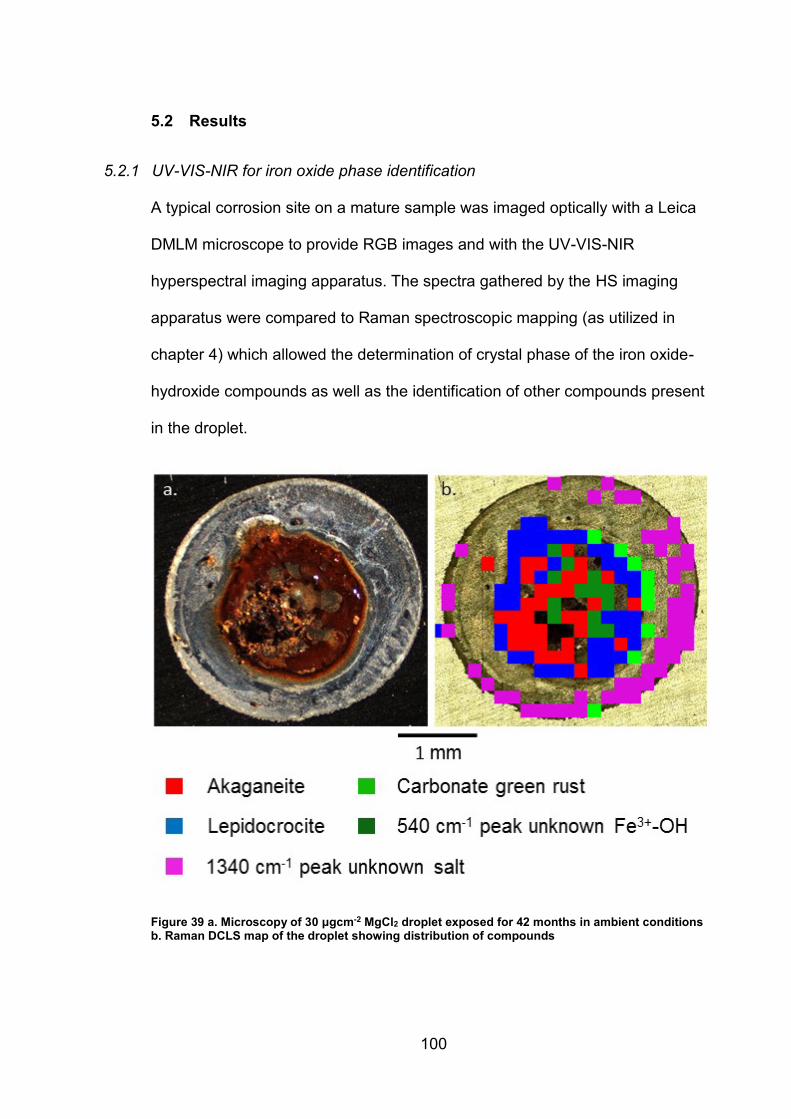
100

5.2 Results

5.2.1 UV-VIS-NIR for iron oxide phase identification

A typical corrosion site on a mature sample was imaged optically with a Leica

DMLM microscope to provide RGB images and with the UV-VIS-NIR

hyperspectral imaging apparatus. The spectra gathered by the HS imaging

apparatus were compared to Raman spectroscopic mapping (as utilized in

chapter 4) which allowed the determination of crystal phase of the iron oxide-

hydroxide compounds as well as the identification of other compounds present

in the droplet.

Figure 39 a. Microscopy of 30 μgcm-2 MgCl2 droplet exposed for 42 months in ambient conditions b. Raman DCLS map of the droplet showing distribution of compounds

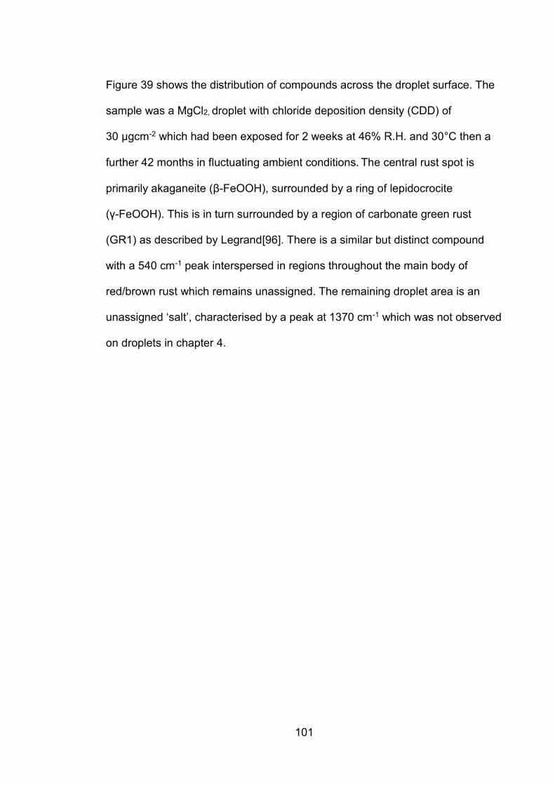
101

Figure 39 shows the distribution of compounds across the droplet surface. The

sample was a MgCl2, droplet with chloride deposition density (CDD) of

30 μgcm-2 which had been exposed for 2 weeks at 46% R.H. and 30°C then a

further 42 months in fluctuating ambient conditions. The central rust spot is

primarily akaganeite (β-FeOOH), surrounded by a ring of lepidocrocite

(γ-FeOOH). This is in turn surrounded by a region of carbonate green rust

(GR1) as described by Legrand[96]. There is a similar but distinct compound

with a 540 cm-1 peak interspersed in regions throughout the main body of

red/brown rust which remains unassigned. The remaining droplet area is an

unassigned ‘salt’, characterised by a peak at 1370 cm-1 which was not observed

on droplets in chapter 4.

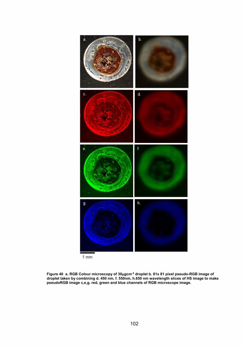
102

Figure 40 a. RGB Colour microscopy of 30µgcm-2 droplet b. 81x 81 pixel pseudo-RGB image of

droplet taken by combining d. 450 nm, f. 550nm, h.650 nm wavelength slices of HS image to make pseudoRGB image c,e,g. red, green and blue channels of RGB microscope image.

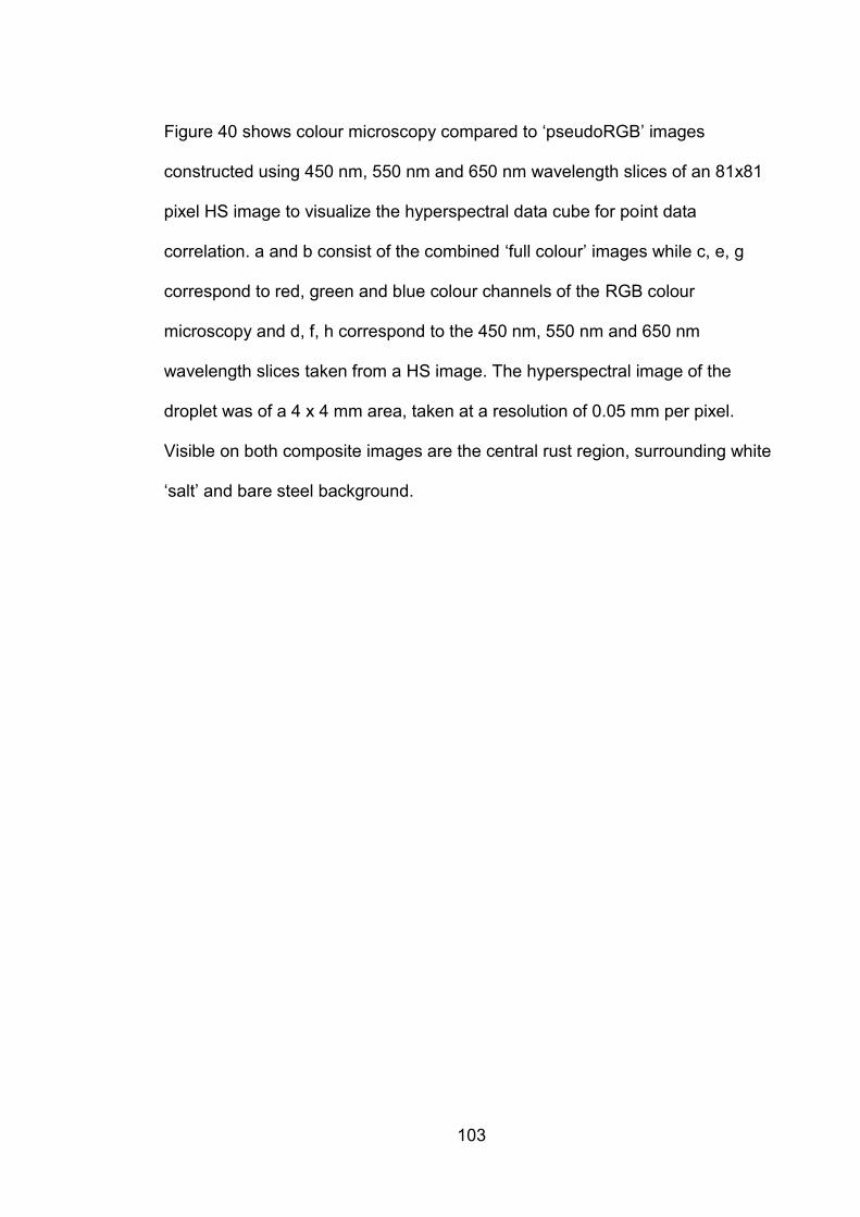
103

Figure 40 shows colour microscopy compared to ‘pseudoRGB’ images

constructed using 450 nm, 550 nm and 650 nm wavelength slices of an 81x81

pixel HS image to visualize the hyperspectral data cube for point data

correlation. a and b consist of the combined ‘full colour’ images while c, e, g

correspond to red, green and blue colour channels of the RGB colour

microscopy and d, f, h correspond to the 450 nm, 550 nm and 650 nm

wavelength slices taken from a HS image. The hyperspectral image of the

droplet was of a 4 x 4 mm area, taken at a resolution of 0.05 mm per pixel.

Visible on both composite images are the central rust region, surrounding white

‘salt’ and bare steel background.

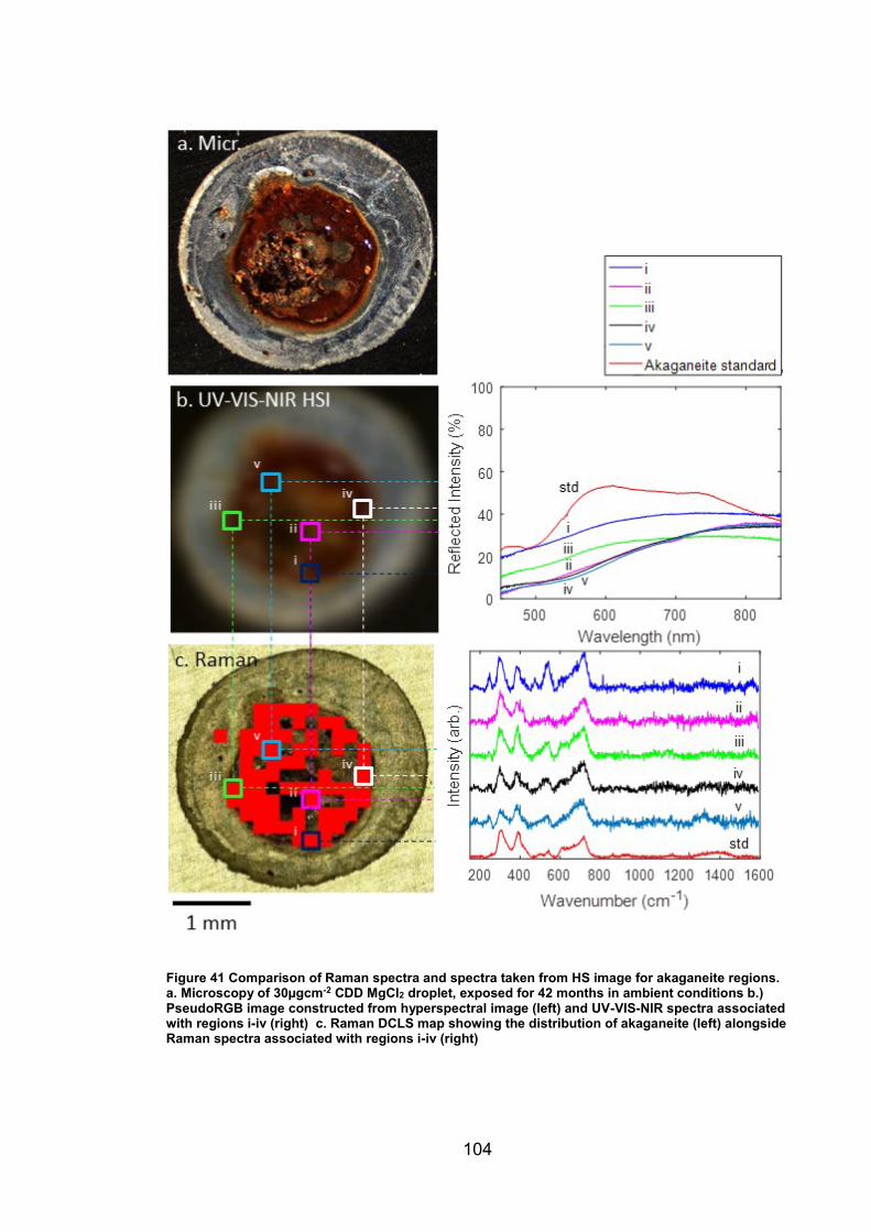
104

Figure 41 Comparison of Raman spectra and spectra taken from HS image for akaganeite regions. a. Microscopy of 30µgcm-2 CDD MgCl2 droplet, exposed for 42 months in ambient conditions b.) PseudoRGB image constructed from hyperspectral image (left) and UV-VIS-NIR spectra associated with regions i-iv (right) c. Raman DCLS map showing the distribution of akaganeite (left) alongside Raman spectra associated with regions i-iv (right)

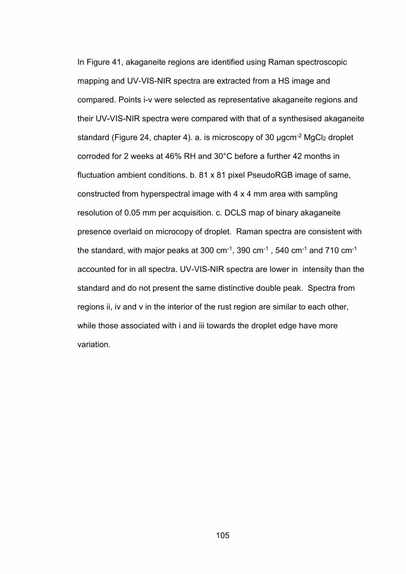
105

In Figure 41, akaganeite regions are identified using Raman spectroscopic

mapping and UV-VIS-NIR spectra are extracted from a HS image and

compared. Points i-v were selected as representative akaganeite regions and

their UV-VIS-NIR spectra were compared with that of a synthesised akaganeite

standard (Figure 24, chapter 4). a. is microscopy of 30 μgcm-2 MgCl2 droplet

corroded for 2 weeks at 46% RH and 30°C before a further 42 months in

fluctuation ambient conditions. b. 81 x 81 pixel PseudoRGB image of same,

constructed from hyperspectral image with 4 x 4 mm area with sampling

resolution of 0.05 mm per acquisition. c. DCLS map of binary akaganeite

presence overlaid on microcopy of droplet. Raman spectra are consistent with

the standard, with major peaks at 300 cm-1, 390 cm-1 , 540 cm-1 and 710 cm-1

accounted for in all spectra. UV-VIS-NIR spectra are lower in intensity than the

standard and do not present the same distinctive double peak. Spectra from

regions ii, iv and v in the interior of the rust region are similar to each other,

while those associated with i and iii towards the droplet edge have more

variation.

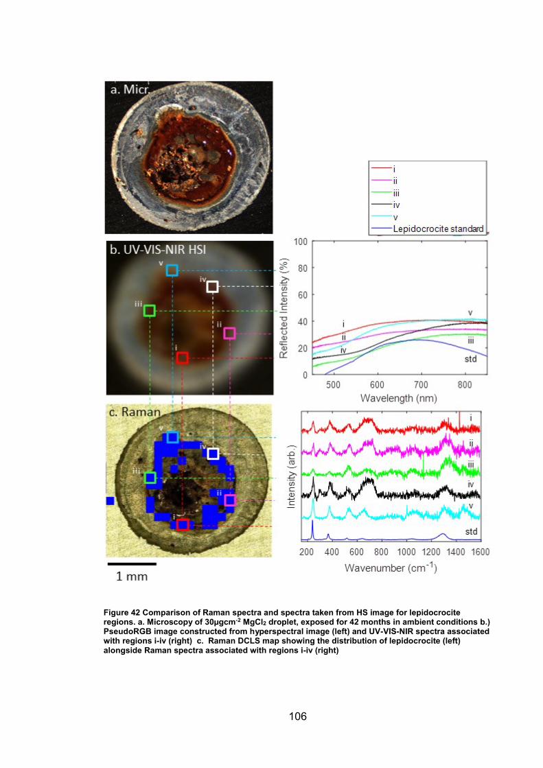
106

Figure 42 Comparison of Raman spectra and spectra taken from HS image for lepidocrocite regions. a. Microscopy of 30µgcm-2 MgCl2 droplet, exposed for 42 months in ambient conditions b.) PseudoRGB image constructed from hyperspectral image (left) and UV-VIS-NIR spectra associated with regions i-iv (right) c. Raman DCLS map showing the distribution of lepidocrocite (left) alongside Raman spectra associated with regions i-iv (right)

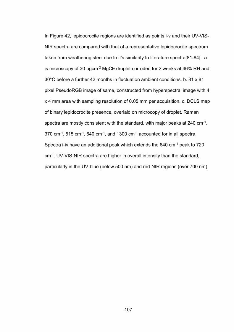
107

In Figure 42, lepidocrocite regions are identified as points i-v and their UV-VIS-

NIR spectra are compared with that of a representative lepidocrocite spectrum

taken from weathering steel due to it’s similarity to literature spectra[81-84] . a.

is microscopy of 30 μgcm-2 MgCl2 droplet corroded for 2 weeks at 46% RH and

30°C before a further 42 months in fluctuation ambient conditions. b. 81 x 81

pixel PseudoRGB image of same, constructed from hyperspectral image with 4

x 4 mm area with sampling resolution of 0.05 mm per acquisition. c. DCLS map

of binary lepidocrocite presence, overlaid on microcopy of droplet. Raman

spectra are mostly consistent with the standard, with major peaks at 240 cm-1,

370 cm-1, 515 cm-1, 640 cm-1, and 1300 cm-1 accounted for in all spectra.

Spectra i-iv have an additional peak which extends the 640 cm-1 peak to 720

cm-1. UV-VIS-NIR spectra are higher in overall intensity than the standard,

particularly in the UV-blue (below 500 nm) and red-NIR regions (over 700 nm).

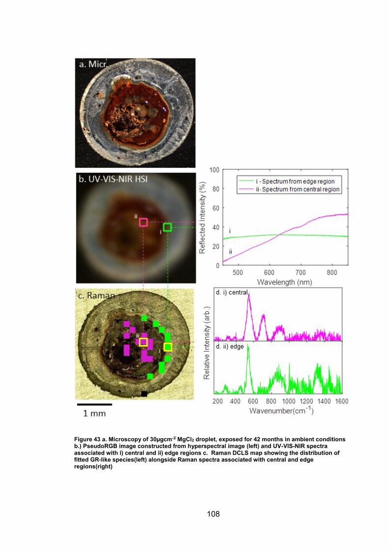
108

Figure 43 a. Microscopy of 30µgcm-2 MgCl2 droplet, exposed for 42 months in ambient conditions b.) PseudoRGB image constructed from hyperspectral image (left) and UV-VIS-NIR spectra associated with i) central and ii) edge regions c. Raman DCLS map showing the distribution of fitted GR-like species(left) alongside Raman spectra associated with central and edge regions(right)

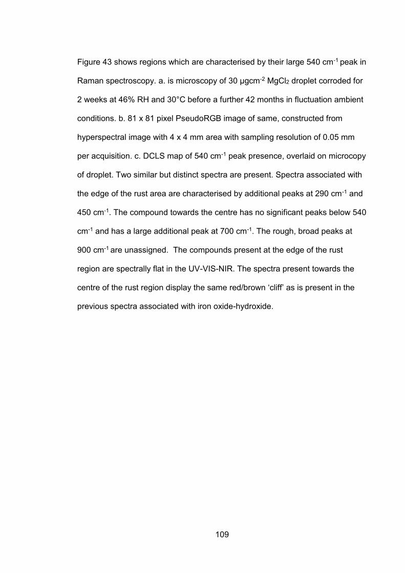
109

Figure 43 shows regions which are characterised by their large 540 cm-1 peak in

Raman spectroscopy. a. is microscopy of 30 μgcm-2 MgCl2 droplet corroded for

2 weeks at 46% RH and 30°C before a further 42 months in fluctuation ambient

conditions. b. 81 x 81 pixel PseudoRGB image of same, constructed from

hyperspectral image with 4 x 4 mm area with sampling resolution of 0.05 mm

per acquisition. c. DCLS map of 540 cm-1 peak presence, overlaid on microcopy

of droplet. Two similar but distinct spectra are present. Spectra associated with

the edge of the rust area are characterised by additional peaks at 290 cm-1 and

450 cm-1. The compound towards the centre has no significant peaks below 540

cm-1 and has a large additional peak at 700 cm-1. The rough, broad peaks at

900 cm-1 are unassigned. The compounds present at the edge of the rust

region are spectrally flat in the UV-VIS-NIR. The spectra present towards the

centre of the rust region display the same red/brown ‘cliff’ as is present in the

previous spectra associated with iron oxide-hydroxide.

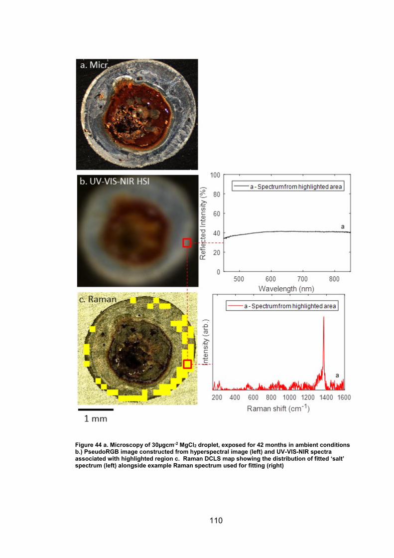
110

Figure 44 a. Microscopy of 30µgcm-2 MgCl2 droplet, exposed for 42 months in ambient conditions b.) PseudoRGB image constructed from hyperspectral image (left) and UV-VIS-NIR spectra associated with highlighted region c. Raman DCLS map showing the distribution of fitted ‘salt’ spectrum (left) alongside example Raman spectrum used for fitting (right)

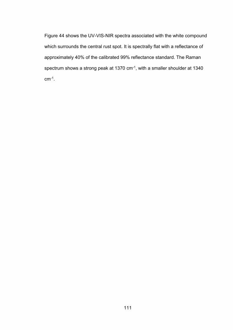
111

Figure 44 shows the UV-VIS-NIR spectra associated with the white compound

which surrounds the central rust spot. It is spectrally flat with a reflectance of

approximately 40% of the calibrated 99% reflectance standard. The Raman

spectrum shows a strong peak at 1370 cm-1, with a smaller shoulder at 1340

cm-1.

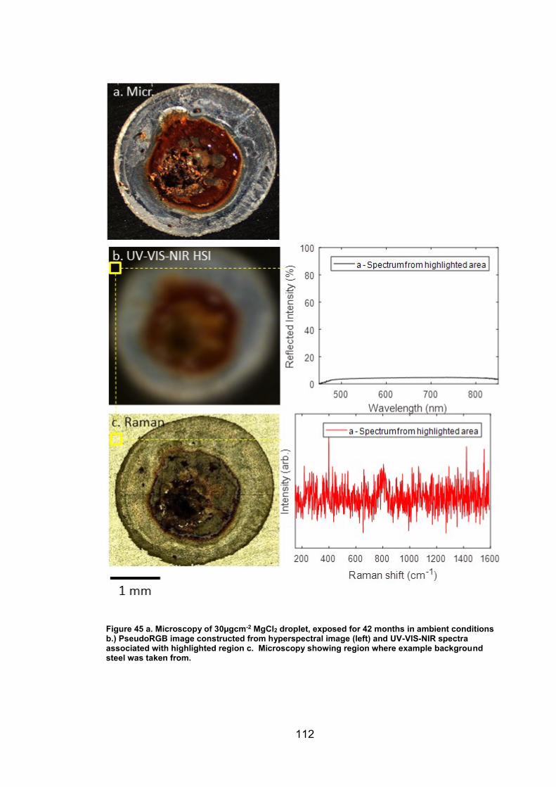
112

Figure 45 a. Microscopy of 30µgcm-2 MgCl2 droplet, exposed for 42 months in ambient conditions b.) PseudoRGB image constructed from hyperspectral image (left) and UV-VIS-NIR spectra associated with highlighted region c. Microscopy showing region where example background steel was taken from.

113

Figure 45 shows UV-VIS-NIR spectra associated with the bare stainless steel

surrounding the droplet. It is spectrally flat with a reflectance of approximately

5% of the 99% calibrated reflectance standard. The Raman spectrum is that of

a typical area of the steel.

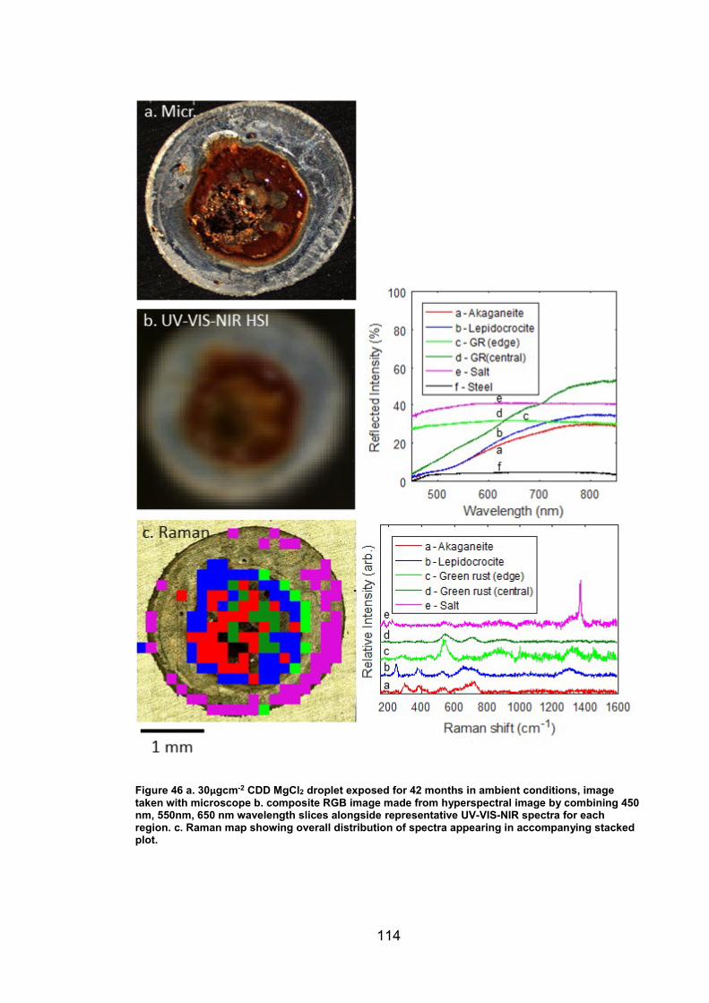
114

Figure 46 a. 30µgcm-2 CDD MgCl2 droplet exposed for 42 months in ambient conditions, image

taken with microscope b. composite RGB image made from hyperspectral image by combining 450 nm, 550nm, 650 nm wavelength slices alongside representative UV-VIS-NIR spectra for each region. c. Raman map showing overall distribution of spectra appearing in accompanying stacked plot.

115

Figure 46 consists of representative examples of all spectra associated with all

measured species. Of note is that the spectra from regions assigned as central

‘green rust’, lepidocrocite and akaganeite spectra are point iv on Figure 42 and

point iii on Figure 41. Spectra are either flat (Figure 46 e,d,f) or have a positive

gradient with a maximum at 800 - 850 nm (Figure 46 a,b,c)

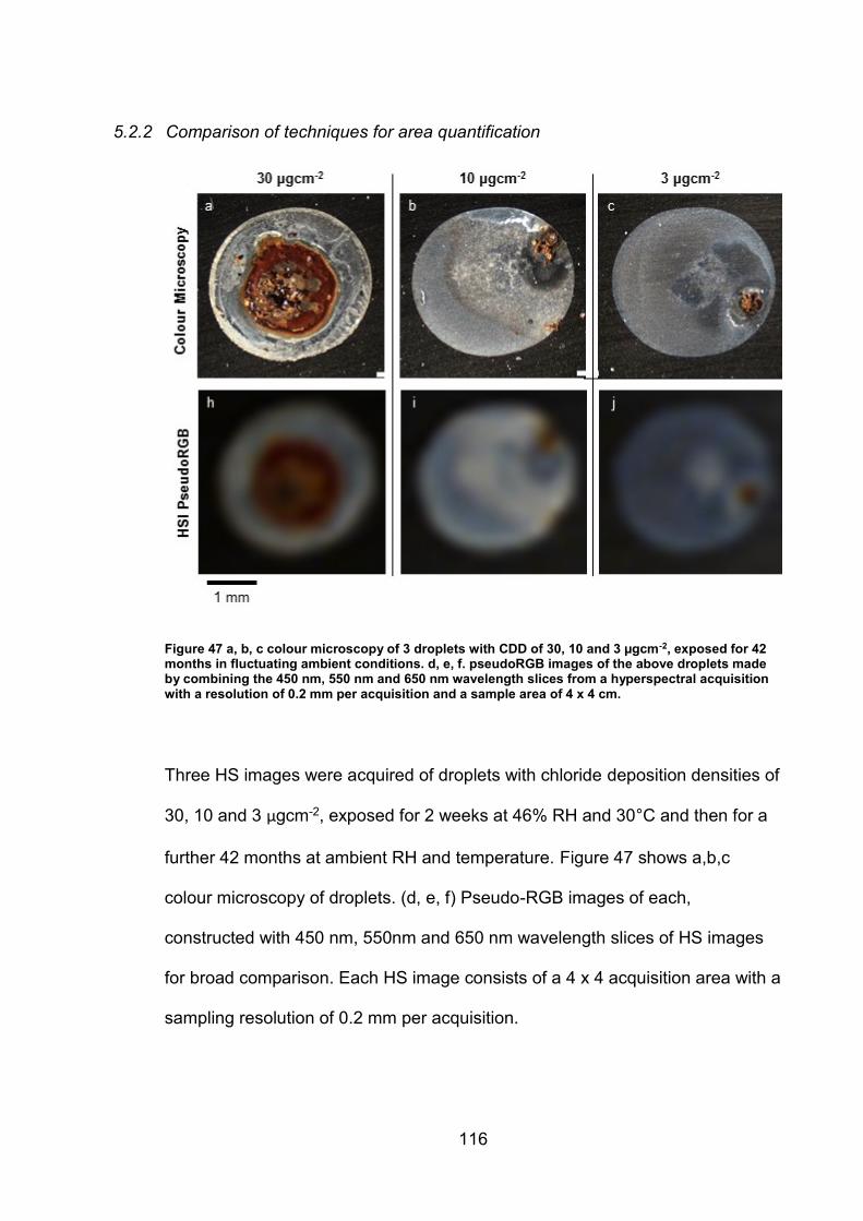
116

5.2.2 Comparison of techniques for area quantification

Figure 47 a, b, c colour microscopy of 3 droplets with CDD of 30, 10 and 3 µgcm-2, exposed for 42 months in fluctuating ambient conditions. d, e, f. pseudoRGB images of the above droplets made by combining the 450 nm, 550 nm and 650 nm wavelength slices from a hyperspectral acquisition with a resolution of 0.2 mm per acquisition and a sample area of 4 x 4 cm.

Three HS images were acquired of droplets with chloride deposition densities of

30, 10 and 3 µgcm-2, exposed for 2 weeks at 46% RH and 30°C and then for a

further 42 months at ambient RH and temperature. Figure 47 shows a,b,c

colour microscopy of droplets. (d, e, f) Pseudo-RGB images of each,

constructed with 450 nm, 550nm and 650 nm wavelength slices of HS images

for broad comparison. Each HS image consists of a 4 x 4 acquisition area with a

sampling resolution of 0.2 mm per acquisition.

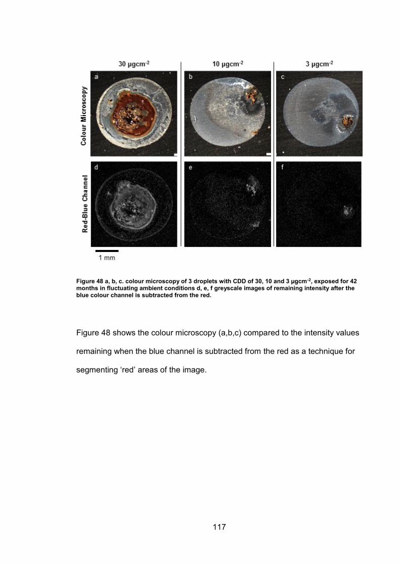
117

Figure 48 a, b, c. colour microscopy of 3 droplets with CDD of 30, 10 and 3 µgcm-2, exposed for 42 months in fluctuating ambient conditions d, e, f greyscale images of remaining intensity after the blue colour channel is subtracted from the red.

Figure 48 shows the colour microscopy (a,b,c) compared to the intensity values

remaining when the blue channel is subtracted from the red as a technique for

segmenting ‘red’ areas of the image.

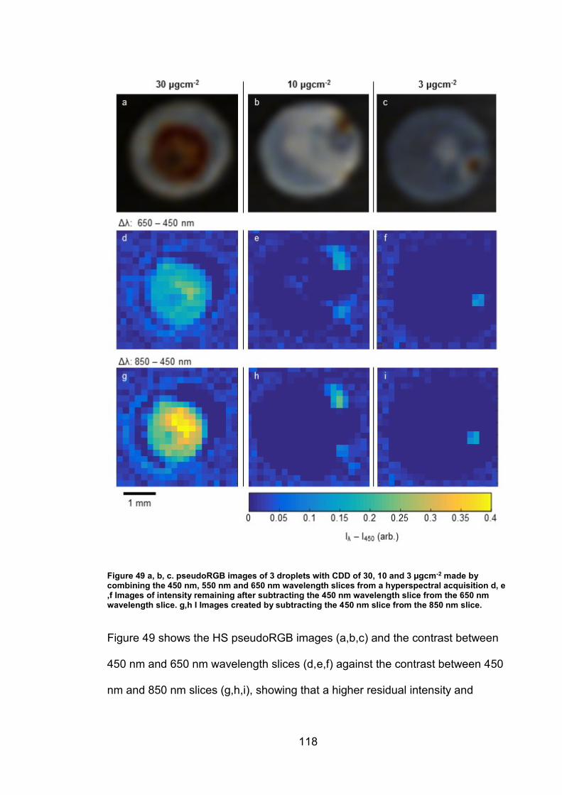
118

Figure 49 a, b, c. pseudoRGB images of 3 droplets with CDD of 30, 10 and 3 µgcm-2 made by combining the 450 nm, 550 nm and 650 nm wavelength slices from a hyperspectral acquisition d, e ,f Images of intensity remaining after subtracting the 450 nm wavelength slice from the 650 nm wavelength slice. g,h I Images created by subtracting the 450 nm slice from the 850 nm slice.

Figure 49 shows the HS pseudoRGB images (a,b,c) and the contrast between

450 nm and 650 nm wavelength slices (d,e,f) against the contrast between 450

nm and 850 nm slices (g,h,i), showing that a higher residual intensity and

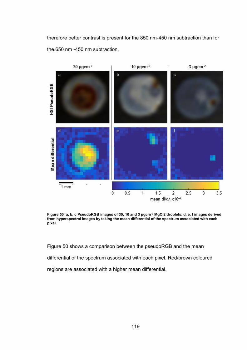
119

therefore better contrast is present for the 850 nm-450 nm subtraction than for

the 650 nm -450 nm subtraction.

Figure 50 a, b, c PseudoRGB images of 30, 10 and 3 μgcm-2 MgCl2 droplets. d, e, f images derived from hyperspectral images by taking the mean differential of the spectrum associated with each pixel.

Figure 50 shows a comparison between the pseudoRGB and the mean

differential of the spectrum associated with each pixel. Red/brown coloured

regions are associated with a higher mean differential.

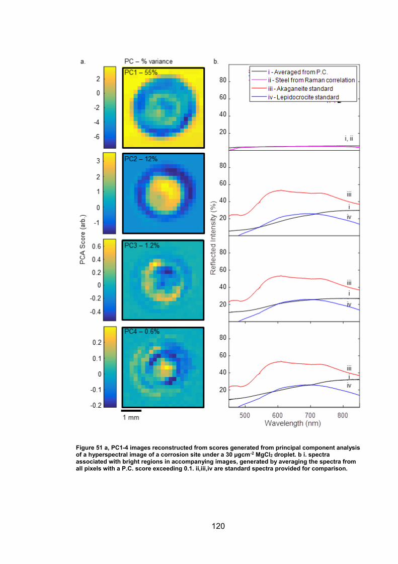
120

Figure 51 a, PC1-4 images reconstructed from scores generated from principal component analysis of a hyperspectral image of a corrosion site under a 30 μgcm-2 MgCl2 droplet. b i. spectra associated with bright regions in accompanying images, generated by averaging the spectra from all pixels with a P.C. score exceeding 0.1. ii,iii,iv are standard spectra provided for comparison.

121

Principal component analysis was performed on the HS image in order to

assess its viability for fast analysis of HS images in a corrosion context. Figure

51 shows the results of principal component analysis of a 21 x 21 pixel

hyperspectral image of a corrosion site under a 30 μgcm-2 MgCl2 droplet,

corroded for 2 weeks at 43% RH and 30°C, followed by 42 months ins

fluctuating ambient conditions. The hyperspectral image is of a 4 x 4 mm area

taken at a sampling resolution of 0.2 mm per acquisition. A. PC1-4 are images

constructed with per pixel scores for each of the first 4 principal components,

accounting for 55% (PC1), 12% (PC2), 1.2% (PC3) and 0.6% (PC4) of the

variance in the dataset. Their corresponding spectra are displayed in b,

gathered by averaging all spectra associated with relevant P.C. and with a

score greater than 0.1. P.C.1 highlights bare steel surrounding the droplet,

P.C.2 highlights the red/brown ‘rust’ region in the central droplet. P.C.3

highlights the yellow tinted region immediately surrounding the main rust region.

P.C.4 highlights the thicker rust layer to the bottom left of the circumference of

the droplet as well as an area of rust at the centre.

122

5.3 Discussion

Apparatus for taking hyperspectral images of droplet sized targets was

assembled and characterised (Section 3.5.2). This apparatus was then used to

take hyperspectral images of mature corrosion sites exposed for 42 months.

The gathered spectra were compared to Raman spectroscopic mapping for

compound identification and phase assignment. Some techniques for

preliminary hyperspectral image analysis were explored.

5.3.1 Iron oxide phase identification using UV-VIS-NIR imaging

Spectra of a mature corrosion site gathered using the hyperspectral apparatus

were compared to Raman spectroscopic mapping for phase analysis. This

distribution can be seen in Figure 39. The corrosion site was under a 30 μgcm-1

CDD MgCl2 droplet, exposed for 2 weeks at 30°C and 46% RH and a further 42

months in fluctuating ambient conditions. An exposure of greater than a month

was desired to ensure relevance to corrosion sites that will be found in

temporary waste stores.

The major constituents of the rust region as seen in Figure 39 were identified as

akaganeite (β-FeOOH) towards the centre of the rust area and lepidocrocite (γ-

FeOOH) around the edge of the rust area, which is typical of MgCl2 droplets

over short term exposures (as seen in Chapter 4). Raman spectra matching

green rust 1 (GR1) as described by Legrand were also observed in the vicinity

immediately surrounding the droplet (Figure 43c)[96]. Some central regions with

a strong 540 cm-1 peak which corresponds to Fe3+-OH[159] and 700 cm-1 peak

corresponding to Fe-O[77, 81, 82] were also observed. The absence of a peak

at 290 cm-1 and 450 cm-1 prevents these central spectra from being assigned as

123

GR1. There was also a strong 1370cm-1 peak associated with the white

compound surrounding the rust region that remains unassigned (Figure 44 c).

This ‘salt’ spectrum was stronger near the droplet edge, indicating that the

crystals were larger and better formed. This likely due to the droplet edge being

first to dry and crystallize during wet-dry cycles as it is where the electrolyte is

thinnest.

In order to aid visualization and correlation between HS images and Raman

maps ‘pseudo-RGB’ images were created by combining 450 nm, 550 nm and

650 nm wavelength slices of the HS image as the red, green and blue

photographs in a colour image. These were then used for matching and

validation of the regions used for correlation with the Raman mapping.

UV-VIS-NIR spectra were then extracted from HS images for regions of each

compound identified by Raman mapping. For points identified as bearing

akaganeite by Raman spectroscopy in Figure 41, no UV-VIS-NIR spectra

present the same intensity distribution as the akaganeite standard (Figure 24),

which has reflectance of 40-60% in the 550-600 nm region, giving it a yellow

hue. Instead the ‘akaganeite’ spectra in the HS image have a reflectance in the

10-30% range. Similarly in Figure 42, no regions of the HS image associated

with lepidocrocite via Raman spectroscopy present UV-VIS-NIR spectra that

match the standard powdered lepidocrocite. There could be several reasons for

this disparity; Synthesized standards were dry and ground into powder whilst

lepidocrocite and akaganeite present in the droplet are precipitated from and

still present alongside the droplet solution meaning particle size, wetting and

arrangement were different for standards and droplet spectra, meaning differing

124

scattering effects between the two. Additionally, the large (~50-100 μm2)

acquisition area of the UV-VIS-NIR illumination makes it likely that several

compounds are illuminated at once, as opposed to the very small region (~10

μm2) gathered during Raman mapping, which would mean that spectra would

be acquired as a mixture.

There are minor regional differences in UV-VIS-NIR spectrum observed for both

crystal phases of iron oxide. For akaganeite in Figure 41, regions ii, iv and v are

consistent with each other despite being from different areas of the droplet,

though all three regions are located towards the interior of the rust region.

Regions i and iii are closer to the edge of the rust region and have a higher

reflectance in the blue-green (450 -550 nm) wavelength interval and a shallower

slope overall. This could be due to spectral blending with light reflected from

outside the rust region due to the large circle of confusion of the illumination.

Regional comparison of lepidocrocite is shown in Figure 42. Significantly more

variation is present in the spectra extracted from HS images due to the regions

of lepidocrocite present on the droplet occurring towards the outer area of the

rust region and so some spectral blending with the surrounding ‘salt’ has

occurred in the HS image. It should be noted that regions i, ii and iv also have

an additional Raman peak at 700 cm-1 usually attributed to Fe-O[157] and an

additional unknown peak at 1500 cm-1. The addition of this Fe-O peak doesn’t

have a reliable effect on the UV-VIS-NIR spectrum however as all measured

display the broad 450-850 nm red/brown slope the same degree.

125

On the edge of the rust region and in the central region there are spectra

characterised by a strong 540 cm-1 peak corresponding to Fe3+-OH[96]. The

spectra around the edge of the rust region match a carbonate green rust that

Legrand describes[96], with an additional sharp peak at 1000 cm-1 which

corresponds to bicarbonate[160] and weaker peaks at 450 cm-1 (Fe2+-OH) and

at 290 cm-1. The UV-VIS-NIR spectrum associated with this region differs very

little from the surrounding salt and does not present a green hue that is usually

associated with green rust. The spectrum associated with the central region is

characterised by an additional peak at 700 cm-1 and significantly reduced 450

cm-1 and 290 cm-1 peaks. The presence of a 700 cm-1 Fe-O band suggests that

this a distinct but similar double layered iron oxide-hydroxide in the fougerite

group rather than Legrand’s green rust 1. This is further supported by the

observed UV-VIS-NIR spectrum presenting the red/brown cliff associated with

akaganeite and lepidocrocite regions across the rest of the droplet. Similar

spectra presenting large 540 cm-1 peaks and small 450 cm-1 peaks are reported

in a paper by Gomez and suggest that it could be due to the uptake of Mg to

form MgFeCO3 or MgFeSO4, but neither carbonate or sulphate peaks are

present between 950 and 1100 cm-1 for central regions[165].

The UV-VIS-NIR salt spectra in Figure 45 are distinct from the surrounding steel

(Figure 46) by virtue of a significantly higher overall reflectance – 30-40% as

opposed to 5-10%, but neither have major spectral features. The Raman

spectrum associated with this ‘salt’ has a single major peak at 1370 cm-1 which

remains unassigned. This suggests that despite lack of spectral features the

126

surface contaminants can be discerned from background steel solely by

reflected intensity rather than any particular spectral band.

5.3.2 Techniques for area quantification/Image analysis

Due to the high dimensionality of the data gathered with a hyperspectral

acquisition, it is necessary to find efficient techniques to both analyse and

visualize the data in an intuitive manner.

Figure 47 shows a comparison between microscopy and ‘pseudoRGB‘ images

of three droplets of CDD 30 μgcm-1, 10 μgcm-1 and 3 μgcm-1, chosen for having

significantly different rust areas. The rust regions are clearly visible as

red/brown pixels. A simple way of segmenting these images for rust area

feature extraction is to highlight red pixels by subtracting the blue channel from

the red, as has been demonstrated in Figure 48 on the colour microscopy

images, and as is commonly utilized as a spectral identifier for iron oxide[5, 117,

166, 167]. This technique is applied to HS images in Figure 49 by subtracting

the 450 nm channel from the 650 nm, with similar results to the microscopy.

Precise area comparison is difficult due to the low spatial resolution of the HS

imager but rusty regions of interest are similarly highlighted. When the same

technique is applied to the 850 nm channel in the near infra-red (Figure 49c) an

average of 65% better contrast is seen over pixels associated with rust region,

suggesting that NIR could significantly improve detectability of small rust

regions. As the peaks are broad, this could be performed with filters i.e. a

multispectral system rather than needing the full spectral range of a HS imaging

system.

127

Another feature extraction technique explored in the Figure 50 is the use of the

mean differential of the spectrum. Higher order differentials are routinely used

for industrial applications[168], but the fact that no sharp features are present in

droplet spectra suggest that higher orders are unnecessary. This is further

supported by the differential method not showing any improvement over colour

channel subtraction for highlighting rusty areas.

Principal component analysis is a method which has been used heavily in

hyperspectral imaging applications for dimensionality reduction as well as for

supervised feature extraction of data due to the technique’s ability to self-order

data along lines of maximum variance, essentially grouping together like

spectra[5, 121, 166, 169, 170]. PCA has been performed on a HS image of a

corrosion site in Figure 51. The first P.C. contrasts the bare metal and the

droplet area as a whole, likely due to bulk reflected intensity differences. The

second P.C. specifically highlights the red/brown rust region due to the positive

intensity gradient associated with the iron oxides present. The majority of the

variance (67%) in the dataset is explained by these first two principal

components, but the third is potentially of note despite the low variance fraction

(1.2%) as it highlights the thinner yellow/orange rust around the exterior of the

rust region, co-incident with the lepidocrocite Raman map. However, the UV-

VIS-NIR spectrum associated with these pixels does not match that of the

standard lepidocrocite. The fourth P.C. corresponds to only 0.6% of the loading

and has no easily discernable spectral features, suggesting that it is not useful

despite it highlighting areas to the edge of the rust ring and centre of the rust

region.

128

In summary, the distinctive red/brown spectrum associated with rust is a

powerful indicator for use in corrosion site detection. The differential in intensity

between the red/NIR (650/850 nm) and the blue (450 nm) allows for simple

feature detection with minimal hardware and software complexity. Hyperspectral

imaging has an advantage in that it provides more reliable intensity information

with a larger spectral range and so could aid with detecting and classifying

unknown non-corrosion related compounds. Unsupervised analysis techniques

such as PCA could also be employed to make use of this increased volume of

data and efficiently segment images with unknown spectra. If complete

automation is the goal, significant attention should be paid to variance fractions

so as to avoid false positives. If a pure corrosion detector is desired, however, it

is not clear that HS + PCA would be any more effective than an arithmetic

colour channel subtraction performed on high resolution colour photography.

While there was a 65% increase in contrast observed by utilizing the 850 nm

wavelength channel over the 650 nm, this would be at the cost of significant

increases in complexity and acquisition time for little gain as all rust was still

detected on the three sites by using colour photography. Single wavelength

optical filters could also be used to take advantage of the extra contrast given

by utilizing the near infra-red without having to invest in HS hardware.

129

5.4 Conclusions

Methods for remote sensing of corrosion products were assessed for their

viability for long term monitoring of corrosion on stainless steel. The expected

corrosion products contain spectral features present in the UV-VIS-NIR region

which are suited for hyperspectral imaging. A system was constructed which

images in the 450 - 850 nm wavelength interval was characterised and

compared to colour photography for detecting corrosion. corrosion product

phase information was verified by Raman spectroscopic mapping.

1. Both UV-VIS-NIR hyperspectral imaging and colour photography were

effective at detecting corrosion site presence from the deposition of rust

around the pit mouth

2. Iron oxide phase identification was not possible using the UV-VIS-NIR

hyperspectral imager, but a positive intensity gradient from 450 nm to

850 nm was associated with the presence of iron oxides and hydroxides.

3. Subtraction of the 450 nm (blue) channel from the 650 nm (red) channel

of RGB colour imagery is adequate for rust region detection, but utilizing

the intensity at 850 nm (NIR), present in the HS image, instead of 650

nm (red) provided 65% better contrast for imaging.

4. HSI has the potential to provide higher contrast for detection of rust, but

at the cost of significantly increased complexity and acquisition time as

colour photography provides the ability to acquire 650 nm and 450 nm

colour channels using off the shelf hardware.

5. Principal component analysis was demonstrated to segment

hyperspectral data of a corrosion site, with PC1 contrasting the

130

background metal with anomalies due to bulk intensity variation and PC2

contrasting rust regions by the red/brown intensity gradient.

131

6. ASSESSMENT OF PIT VOLUME WITH RESPECT TO VISIBLE RUST

AREA

6.1 Introduction

Corrosion attack is usually quantified by metal loss, either by weight or by

volume, but metal loss for pitting is small which presents a challenge for

inspection efforts. Standard methodology for assessing pitting attack is based

on labour intensive individual close inspection of the attack sites, with surfaces

being cleaned of corrosion product before inspection[171]. During atmospheric

pitting all rust generated will be retained in the immediate vicinity of the

corrosion site, suggesting that quantifying metal attack by measuring visible rust

is possible. To date there has been no quantification of visible rust with respect

to a metric for metal loss.

In this chapter, this relationship is investigated for salts relevant nuclear waste

stores (MgCl2, CaCl2), chloride deposition density (CDD) (<100 μgcm-2) and

conditions(fluctuating, 20-30°C and 20-50% RH)[9] by comparing rust area

measurements from colour photography to pit volume information gathered by

confocal laser scanning microscopy.

Colour based image segmentation techniques are widespread in industry and

has been previously proposed for corrosion detection[110, 136, 137]. Four

colour based image processing techniques (outlined in sections 3.6.1 to 3.6.4)

are compared for their efficacy at rust detection:

Red-Blue colour channel subtraction of the RGB image, followed by

thresholding of the remaining intensity. This was chosen due to its

132

simplicity of application, requiring only two matrix operations to fully

segment the image.

Principal component analysis (PCA) of the RGB image, followed by

thresholding of the score of the second principal component. PCA is an

unsupervised technique in wide use for anomaly detection and semi-

automated segmentation of RGB colour and hyperspectral images in

industry[141, 144, 170, 172, 173].

Conversion to HSV colour space followed by thresholding of the hue and

saturation indices. Use of HSV colour space allows for thresholding to be

performed using criteria which are more intuitive to a user. Chroma (Hue)

is separated from saturation(S) and brightness (Value), allowing for the

selection of colour independent of lighting condition.

Conversion 1976 CIELAB (L*a*b*) colour space, followed by thresholding

of the b* (green-yellow) index. L*a*b* colour space was designed to be

both device independent and perceptually uniform, meaning that the

technique should be more robust when using data gathered using

different instruments and that the supervised thresholding process

should be more consistent.

133

6.2 Results

MgCl2 and CaCl2 droplets of 100, 50 and 20 µgcm-2 chloride deposition density

were deposited on 304L stainless steel and exposed for 14 days in either fixed

46% RH and 30°C conditions or fluctuating ambient conditions between 19-

49% RH and 19-24°C to provide a range of rust areas and pit volumes. 73

MgCl2 and 74 CaCl2 droplets with pits were analysed. After exposure, colour

photographs were taken before the corrosion product was removed and

confocal laser scanning confocal microscopy was performed to measure pit

volume.

Four segmentation techniques were used to separate rust area from other

surface features in the colour photographs:

Red-Blue colour channel subtraction of the RGB image, followed by

thresholding of the remaining intensity

Principal component analysis (PCA) of the RGB image, followed by

thresholding of the score of the second principal component

Conversion to HSV colour space, followed by thresholding of the hue

and saturation indices

Conversion to L*a*b* colour space, followed by thresholding of the b*

(green-yellow) index.

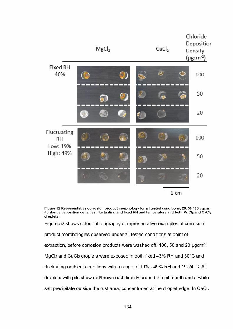
134

Figure 52 Representative corrosion product morphology for all tested conditions; 20, 50 100 μgcm-

2 chloride deposition densities, fluctuating and fixed RH and temperature and both MgCl2 and CaCl2

droplets.

Figure 52 shows colour photography of representative examples of corrosion

product morphologies observed under all tested conditions at point of

extraction, before corrosion products were washed off. 100, 50 and 20 µgcm-2

MgCl2 and CaCl2 droplets were exposed in both fixed 43% RH and 30°C and

fluctuating ambient conditions with a range of 19% - 49% RH and 19-24°C. All

droplets with pits show red/brown rust directly around the pit mouth and a white

salt precipitate outside the rust area, concentrated at the droplet edge. In CaCl2

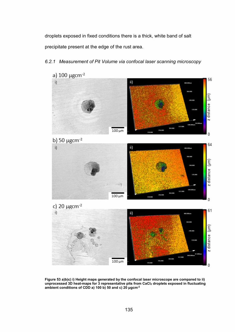
135

droplets exposed in fixed conditions there is a thick, white band of salt

precipitate present at the edge of the rust area.

6.2.1 Measurement of Pit Volume via confocal laser scanning microscopy

Figure 53 a)b)c) i) Height maps generated by the confocal laser microscope are compared to ii) unprocessed 3D heat-maps for 3 representative pits from CaCl2 droplets exposed in fluctuating ambient conditions of CDD a) 100 b) 50 and c) 20 μgcm-2

136

After exposure, the samples were photographed, rinsed and ultrasonically

cleaned in deionized water to remove corrosion products. Laser scanning

confocal microscopy was then used to measure pit volumes. Figure 53 shows

a) i,b) i , c)i intensity height map produced by the confocal microscopy in

relation to the raw 3D heat map produced by the software. a), b), c) ii.

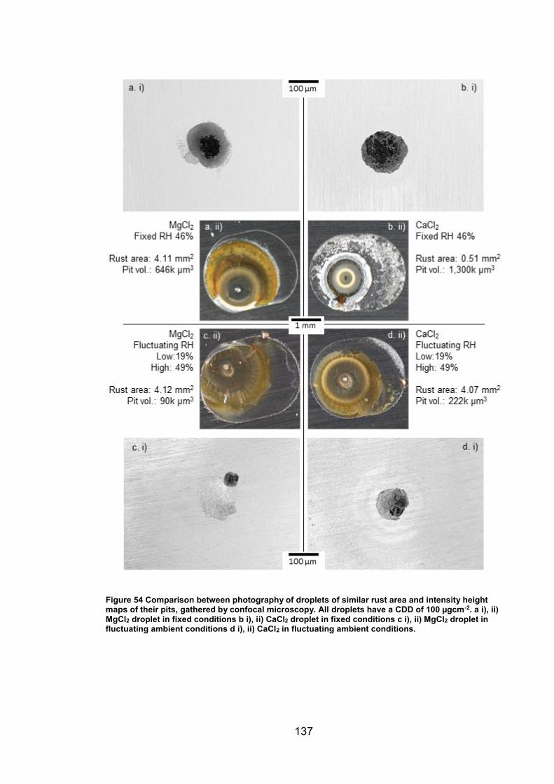
137

Figure 54 Comparison between photography of droplets of similar rust area and intensity height maps of their pits, gathered by confocal microscopy. All droplets have a CDD of 100 µgcm-2. a i), ii) MgCl2 droplet in fixed conditions b i), ii) CaCl2 droplet in fixed conditions c i), ii) MgCl2 droplet in fluctuating ambient conditions d i), ii) CaCl2 in fluctuating ambient conditions.

138

Figure 54 shows photography of a representative set of 100 µgcm-2 CDD

droplets of similar rust area for all tested conditions and associated confocal

microscopy images showing pit morphology. In the case of the CaCl2 droplet

(b), a site was chosen with a large pit volume as no valid droplet was available

with similar rust area to the other sites. All other droplets have different pit

volumes, despite having near identical rust area. Several pit morphologies are

present. a and b i) showing hemispherical morphology while c and d i) show a

shallow dish with a spiral morphology.

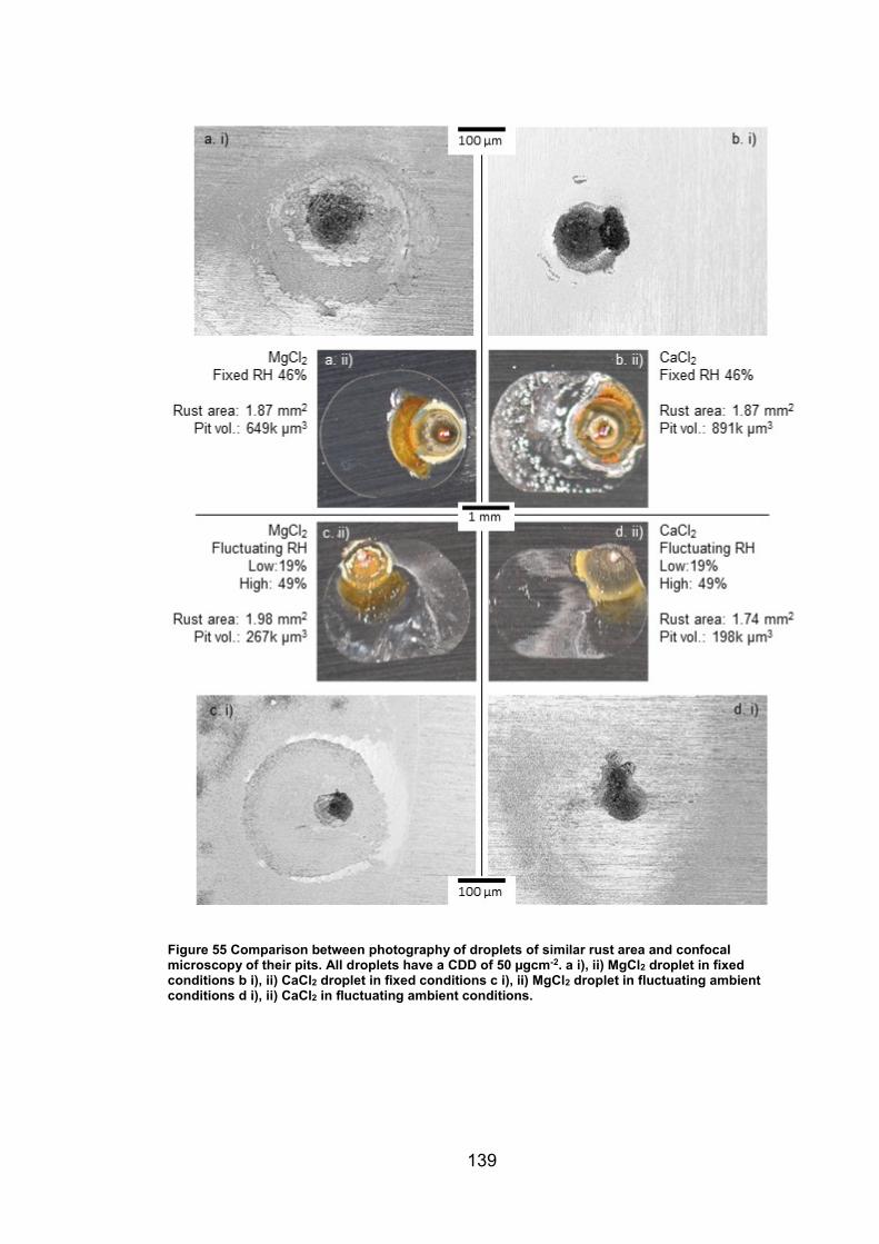
139

Figure 55 Comparison between photography of droplets of similar rust area and confocal microscopy of their pits. All droplets have a CDD of 50 µgcm-2. a i), ii) MgCl2 droplet in fixed conditions b i), ii) CaCl2 droplet in fixed conditions c i), ii) MgCl2 droplet in fluctuating ambient conditions d i), ii) CaCl2 in fluctuating ambient conditions.

140

Figure 55 shows photography of a representative set of 50 µgcm-2 CDD

droplets of similar rust area for all tested conditions and associated confocal

microscopy images showing pit morphology. All pits show a hemispherical

morphology.

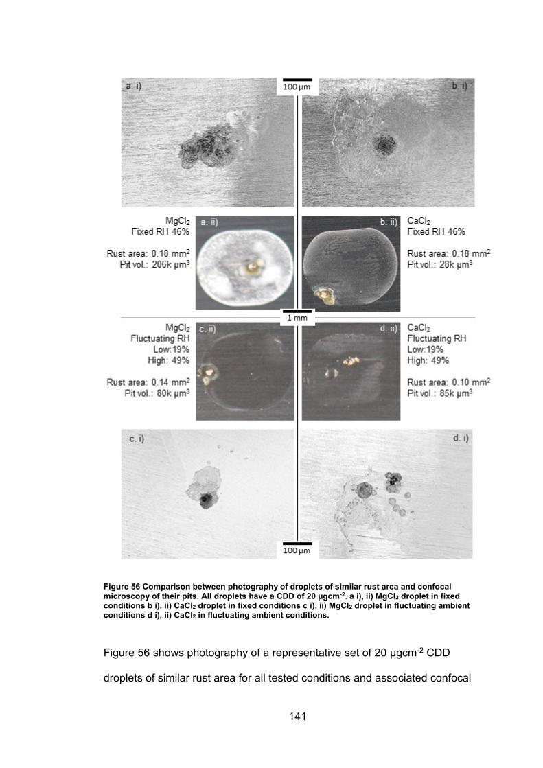
141

Figure 56 Comparison between photography of droplets of similar rust area and confocal microscopy of their pits. All droplets have a CDD of 20 µgcm-2. a i), ii) MgCl2 droplet in fixed conditions b i), ii) CaCl2 droplet in fixed conditions c i), ii) MgCl2 droplet in fluctuating ambient conditions d i), ii) CaCl2 in fluctuating ambient conditions.

Figure 56 shows photography of a representative set of 20 µgcm-2 CDD

droplets of similar rust area for all tested conditions and associated confocal

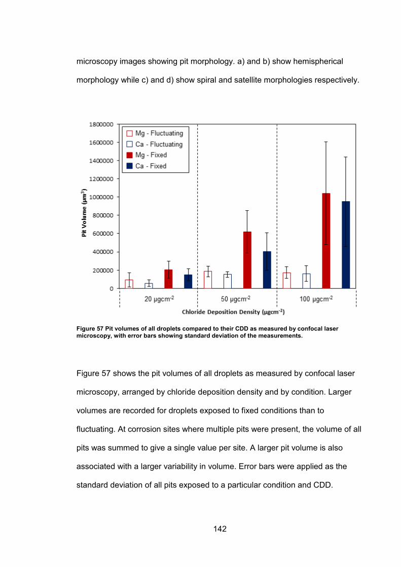
142

microscopy images showing pit morphology. a) and b) show hemispherical

morphology while c) and d) show spiral and satellite morphologies respectively.

Figure 57 Pit volumes of all droplets compared to their CDD as measured by confocal laser microscopy, with error bars showing standard deviation of the measurements.

Figure 57 shows the pit volumes of all droplets as measured by confocal laser

microscopy, arranged by chloride deposition density and by condition. Larger

volumes are recorded for droplets exposed to fixed conditions than to

fluctuating. At corrosion sites where multiple pits were present, the volume of all

pits was summed to give a single value per site. A larger pit volume is also

associated with a larger variability in volume. Error bars were applied as the

standard deviation of all pits exposed to a particular condition and CDD.

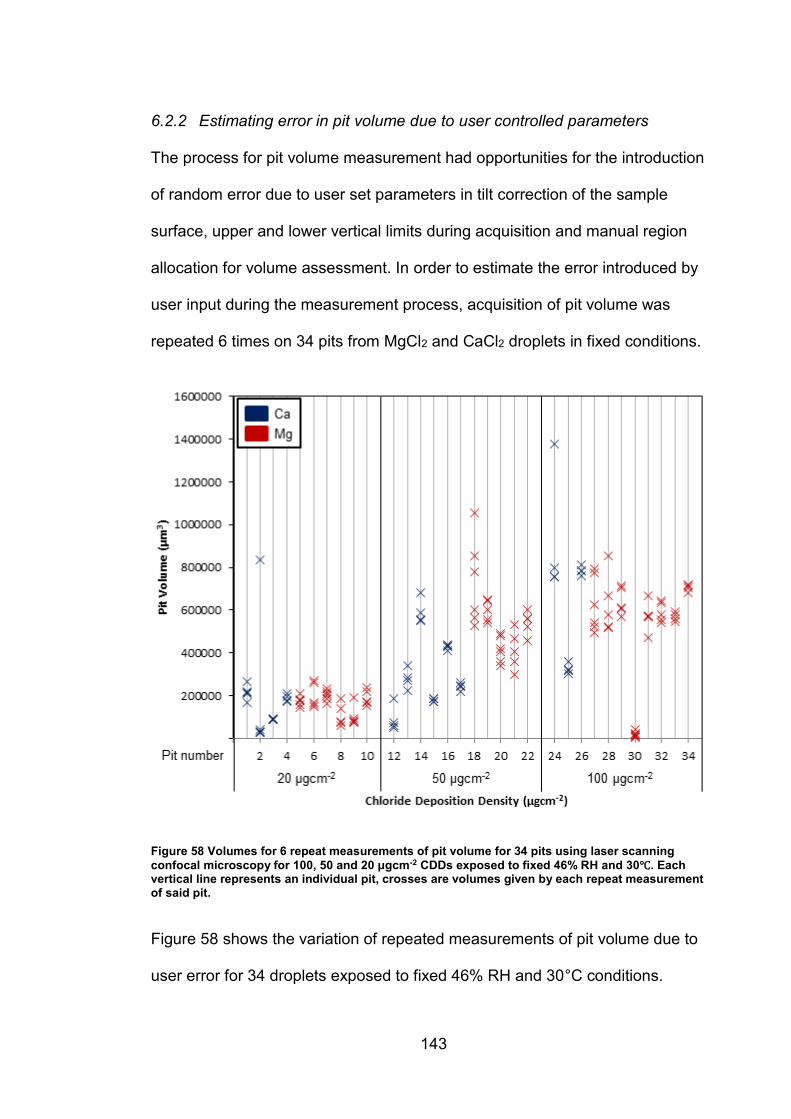
143

6.2.2 Estimating error in pit volume due to user controlled parameters

The process for pit volume measurement had opportunities for the introduction

of random error due to user set parameters in tilt correction of the sample

surface, upper and lower vertical limits during acquisition and manual region

allocation for volume assessment. In order to estimate the error introduced by

user input during the measurement process, acquisition of pit volume was

repeated 6 times on 34 pits from MgCl2 and CaCl2 droplets in fixed conditions.

Figure 58 Volumes for 6 repeat measurements of pit volume for 34 pits using laser scanning

confocal microscopy for 100, 50 and 20 μgcm-2 CDDs exposed to fixed 46% RH and 30℃. Each vertical line represents an individual pit, crosses are volumes given by each repeat measurement of said pit.

Figure 58 shows the variation of repeated measurements of pit volume due to

user error for 34 droplets exposed to fixed 46% RH and 30°C conditions.

144

Table 8 Breakdown of standard deviation as averaged percentage of the mean associated pit measurement by salt cation and chloride deposition density for all 34 pits present in Figure 58

Salt Cation Chloride Deposition density (μgcm-2)

All CDDs 100 50 20

Mg 16% 12% 23% 18%

Ca 8% 16% 14% 17%

Table 8 shows the averaged percentage standard deviation present in the

measurement of pit volume for 34 pits exposed to fixed conditions. Standard

deviations are shown as an averaged percentage of the mean of all

measurements for a particular chloride deposition density, salt cation or

combination of the two.

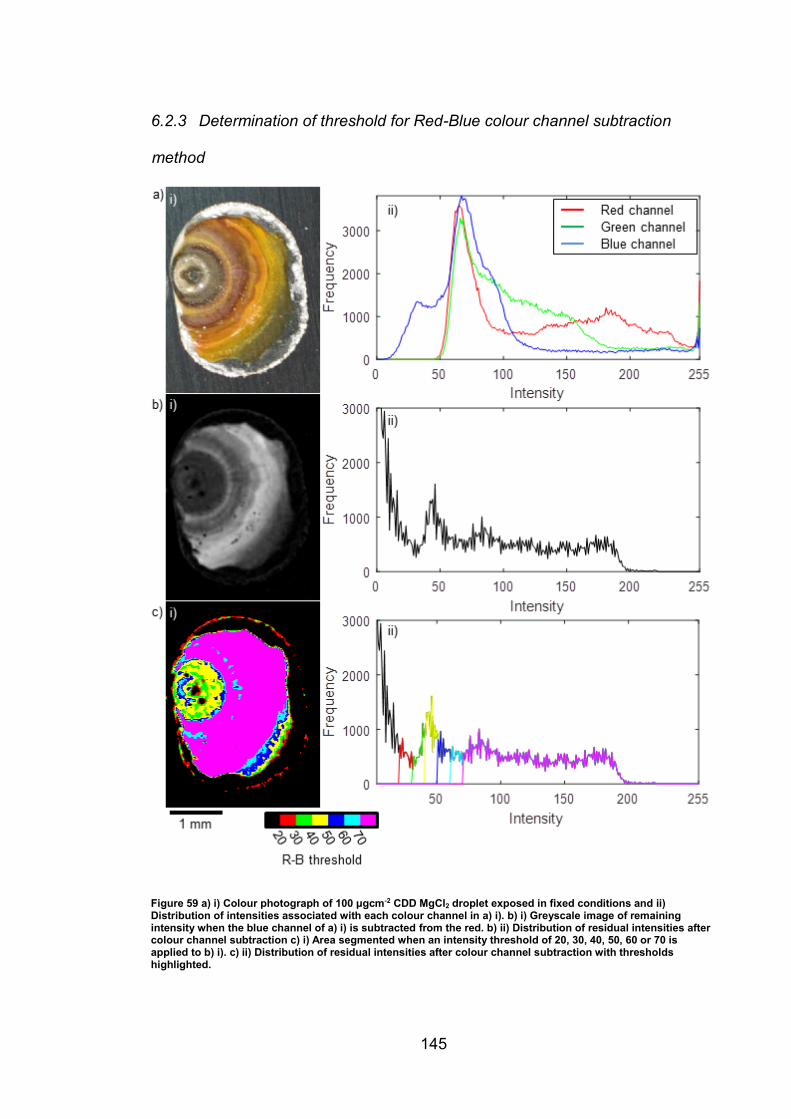
145

6.2.3 Determination of threshold for Red-Blue colour channel subtraction

method

Figure 59 a) i) Colour photograph of 100 μgcm-2 CDD MgCl2 droplet exposed in fixed conditions and ii) Distribution of intensities associated with each colour channel in a) i). b) i) Greyscale image of remaining intensity when the blue channel of a) i) is subtracted from the red. b) ii) Distribution of residual intensities after colour channel subtraction c) i) Area segmented when an intensity threshold of 20, 30, 40, 50, 60 or 70 is applied to b) i). c) ii) Distribution of residual intensities after colour channel subtraction with thresholds highlighted.

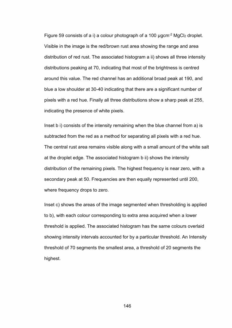
146

Figure 59 consists of a i) a colour photograph of a 100 μgcm-2 MgCl2 droplet.

Visible in the image is the red/brown rust area showing the range and area

distribution of red rust. The associated histogram a ii) shows all three intensity

distributions peaking at 70, indicating that most of the brightness is centred

around this value. The red channel has an additional broad peak at 190, and

blue a low shoulder at 30-40 indicating that there are a significant number of

pixels with a red hue. Finally all three distributions show a sharp peak at 255,

indicating the presence of white pixels.

Inset b i) consists of the intensity remaining when the blue channel from a) is

subtracted from the red as a method for separating all pixels with a red hue.

The central rust area remains visible along with a small amount of the white salt

at the droplet edge. The associated histogram b ii) shows the intensity

distribution of the remaining pixels. The highest frequency is near zero, with a

secondary peak at 50. Frequencies are then equally represented until 200,

where frequency drops to zero.

Inset c) shows the areas of the image segmented when thresholding is applied

to b), with each colour corresponding to extra area acquired when a lower

threshold is applied. The associated histogram has the same colours overlaid

showing intensity intervals accounted for by a particular threshold. An Intensity

threshold of 70 segments the smallest area, a threshold of 20 segments the

highest.

147

6.2.4 Determination of threshold for principal component analysis method

Figure 60 a) i) Colour photograph of 100 μgcm-2 CDD MgCl2 droplet exposed in fixed conditions and ii) Distribution of intensities associated with each colour channel in a) i). b) i-iii) 1st, 2nd and 3rd principal components of a) i). c) i) Distribution of scores in the 2nd principal component c) ii) histogram of scores of the 2nd principal component. d) i) Areas segmented when score threshold is applied to the second principal component d ii) distribution of intensities segmented with a particular threshold.

148

Figure 60 consists of a i) a colour photograph of a 100 μgcm-2 MgCl2 droplet.

Visible in the image is the red/brown rust area showing the range and area

distribution of red rust. The associated histogram a ii) shows all three intensity

distributions peaking at 70. The red channel has an additional broad peak at

190, the green channel has a large shoulder from 70 to 170 and the blue

channel has two shoulders at 40 and 100 either side of the main peak at 70.

Finally all three distributions show a sharp peak at 255.

b i-iii) shows heat maps of the 1st, 2nd and 3rd principal components of the image

in a) The first principal component highlights the variation in overall intensity

with the bright white salt around the droplet being given a low score and the rest

of the image approximately equal. In the second principal component the rusty

region is highlighted with a lighter yellow rust colour associated with a higher

score. The third principal component highlights visible rust with a deeper red-

brown rust colour associated with a higher score. c i) shows a zoom of the 2nd

principal component and the associated histogram cii) shows the score

distribution. It has a large peak in score at -20 with the rest of the distribution

being approximately equal in frequency up to a score of 80, where it drops to

zero.

The image d i) and associated histogram d ii) are the product of score

thresholding of the second principal component showing the regions contained

within each score interval. A threshold of -20 includes significant non- rusty

pixels, a threshold of zero maximizes segmentation of rusty area.

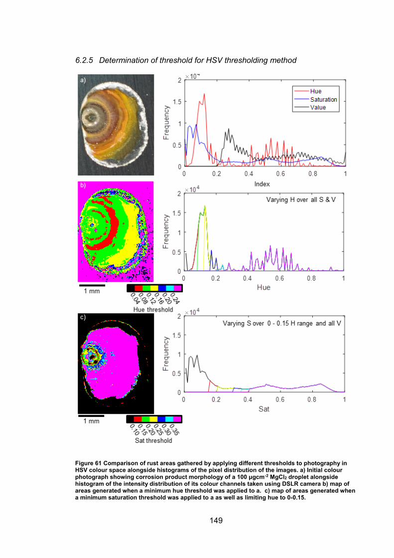
149

6.2.5 Determination of threshold for HSV thresholding method

Figure 61 Comparison of rust areas gathered by applying different thresholds to photography in HSV colour space alongside histograms of the pixel distribution of the images. a) Initial colour photograph showing corrosion product morphology of a 100 μgcm-2 MgCl2 droplet alongside histogram of the intensity distribution of its colour channels taken using DSLR camera b) map of areas generated when a minimum hue threshold was applied to a. c) map of areas generated when a minimum saturation threshold was applied to a as well as limiting hue to 0-0.15.

150

Figure 61 consists of a) colour photograph of a 100 μgcm-2 MgCl2 droplet

alongside the histogram of the hue, saturation and value distributions. The

major feature in hue is a large peak at 0-0.15. Saturation is largest close to 0

with minor peaks at 0.5 and 0.8. Value is zero below 0.2, peaks at 0.3 and has

a very broad peak centred at 0.7. Inset b) shows the areas associated with

different values of hue. All areas are included with a value over 0.2, while

progressively smaller regions of the total rusty area are included with lower

thresholds. Inset c) shows the areas gathered when saturation thresholds are

applied to an image trimmed to 0-0.15 in hue. All thresholds include the rust

area but saturations below 0.3 also include parts of the white salt at the edge of

the droplet.

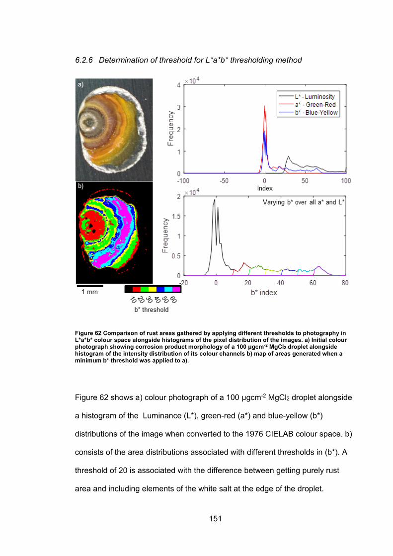
151

6.2.6 Determination of threshold for L*a*b* thresholding method

Figure 62 Comparison of rust areas gathered by applying different thresholds to photography in L*a*b* colour space alongside histograms of the pixel distribution of the images. a) Initial colour photograph showing corrosion product morphology of a 100 μgcm-2 MgCl2 droplet alongside histogram of the intensity distribution of its colour channels b) map of areas generated when a minimum b* threshold was applied to a).

Figure 62 shows a) colour photograph of a 100 μgcm-2 MgCl2 droplet alongside

a histogram of the Luminance (L*), green-red (a*) and blue-yellow (b*)

distributions of the image when converted to the 1976 CIELAB colour space. b)

consists of the area distributions associated with different thresholds in (b*). A

threshold of 20 is associated with the difference between getting purely rust

area and including elements of the white salt at the edge of the droplet.

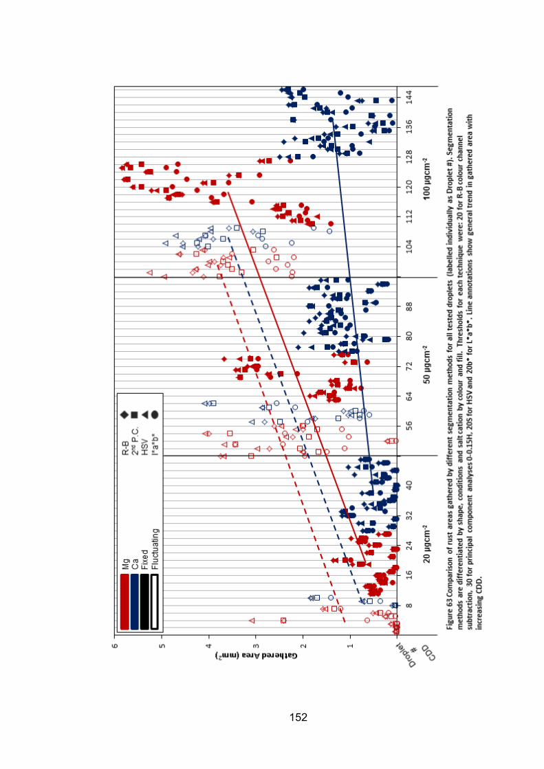
152

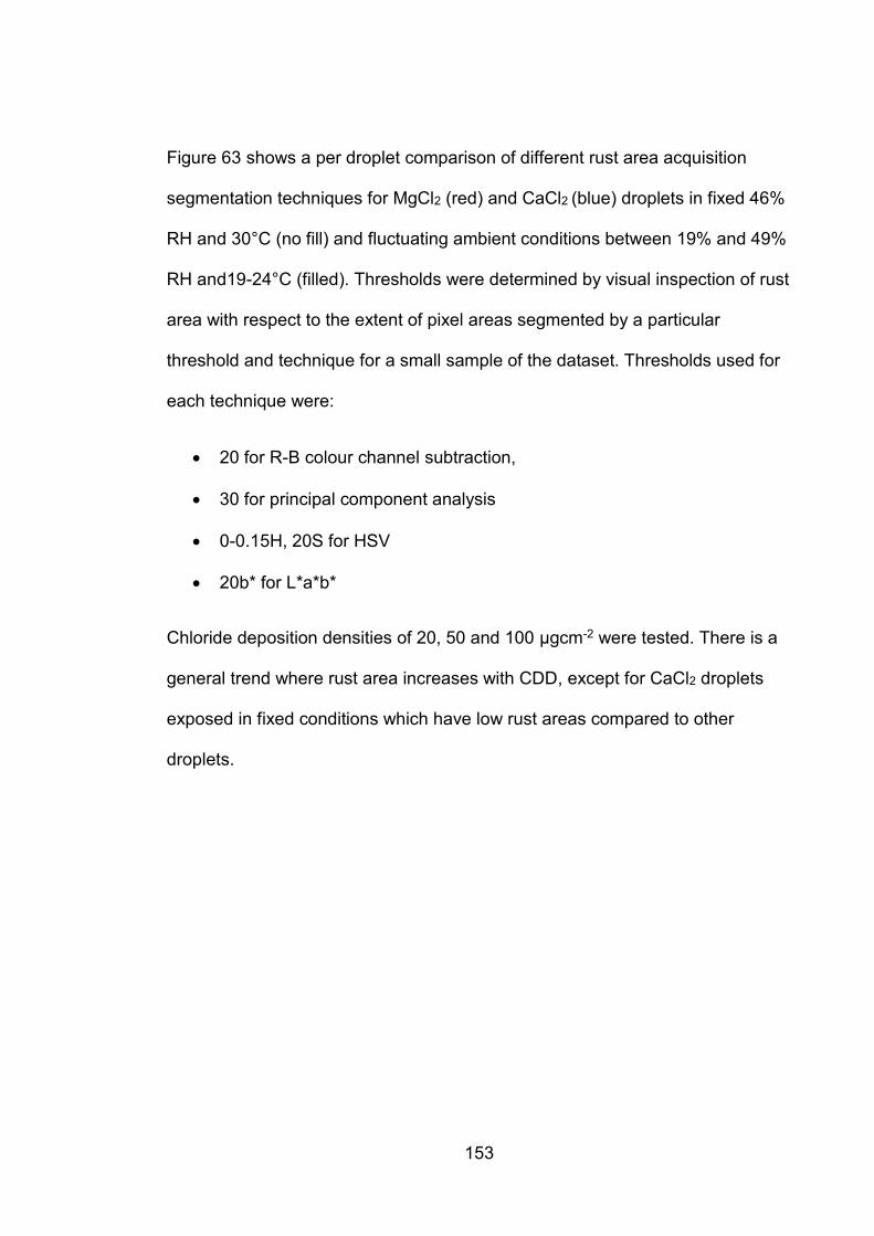
153

Figure 63

Figure 63 shows a per droplet comparison of different rust area acquisition

segmentation techniques for MgCl2 (red) and CaCl2 (blue) droplets in fixed 46%

RH and 30°C (no fill) and fluctuating ambient conditions between 19% and 49%

RH and19-24°C (filled). Thresholds were determined by visual inspection of rust

area with respect to the extent of pixel areas segmented by a particular

threshold and technique for a small sample of the dataset. Thresholds used for

each technique were:

20 for R-B colour channel subtraction,

30 for principal component analysis

0-0.15H, 20S for HSV

20b* for L*a*b*

Chloride deposition densities of 20, 50 and 100 μgcm-2 were tested. There is a

general trend where rust area increases with CDD, except for CaCl2 droplets

exposed in fixed conditions which have low rust areas compared to other

droplets.

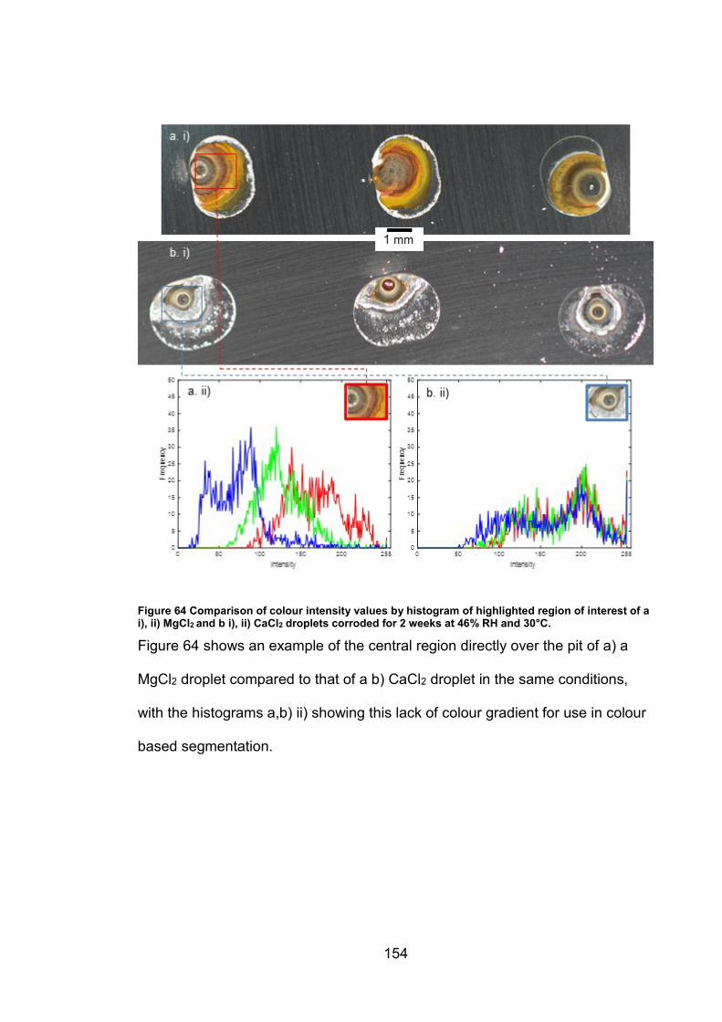
154

Figure 64 Comparison of colour intensity values by histogram of highlighted region of interest of a i), ii) MgCl2 and b i), ii) CaCl2 droplets corroded for 2 weeks at 46% RH and 30°C.

Figure 64 shows an example of the central region directly over the pit of a) a

MgCl2 droplet compared to that of a b) CaCl2 droplet in the same conditions,

with the histograms a,b) ii) showing this lack of colour gradient for use in colour

based segmentation.

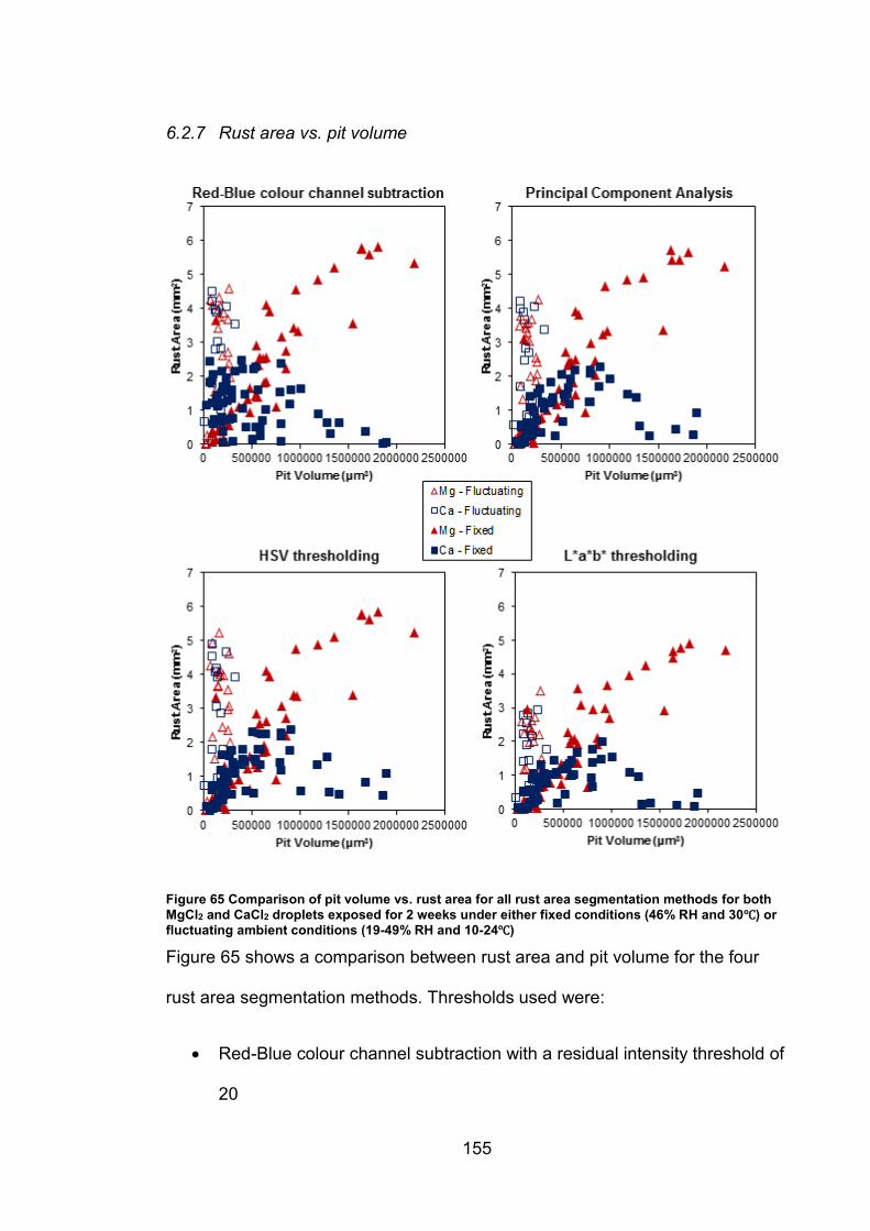
155

6.2.7 Rust area vs. pit volume

Figure 65 Comparison of pit volume vs. rust area for all rust area segmentation methods for both

MgCl2 and CaCl2 droplets exposed for 2 weeks under either fixed conditions (46% RH and 30℃) or

fluctuating ambient conditions (19-49% RH and 10-24℃)

Figure 65 shows a comparison between rust area and pit volume for the four

rust area segmentation methods. Thresholds used were:

Red-Blue colour channel subtraction with a residual intensity threshold of

20

156

2nd principal component score of 30 for the PCA method.

HSV threshold of 0.15 hue and 0.2 saturation

b* threshold of 20 for L*a*b* thresholding

All four methods present a broadly linear relationship for droplets exposed in

fixed 46% RH and 30℃, while droplets exposed in fluctuating ambient

conditions (19-49% RH and 10-24℃) are limited to pit volumes of less than

400,000 μm3 despite having a similar spread of rust areas to the droplets

exposed to fixed conditions. CaCl2 droplets with pit volumes over 1,000,000

μm3 had significantly lower rust areas than would be expected from a linear

relationship.

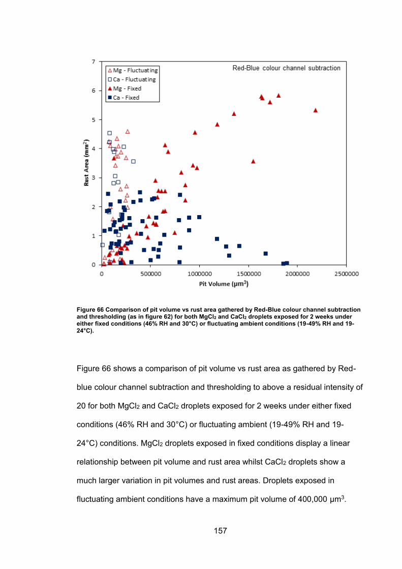
157

Figure 66 Comparison of pit volume vs rust area gathered by Red-Blue colour channel subtraction and thresholding (as in figure 62) for both MgCl2 and CaCl2 droplets exposed for 2 weeks under either fixed conditions (46% RH and 30°C) or fluctuating ambient conditions (19-49% RH and 19-24°C).

Figure 66 shows a comparison of pit volume vs rust area as gathered by Red-

blue colour channel subtraction and thresholding to above a residual intensity of

20 for both MgCl2 and CaCl2 droplets exposed for 2 weeks under either fixed

conditions (46% RH and 30°C) or fluctuating ambient (19-49% RH and 19-

24°C) conditions. MgCl2 droplets exposed in fixed conditions display a linear

relationship between pit volume and rust area whilst CaCl2 droplets show a

much larger variation in pit volumes and rust areas. Droplets exposed in

fluctuating ambient conditions have a maximum pit volume of 400,000 μm3.

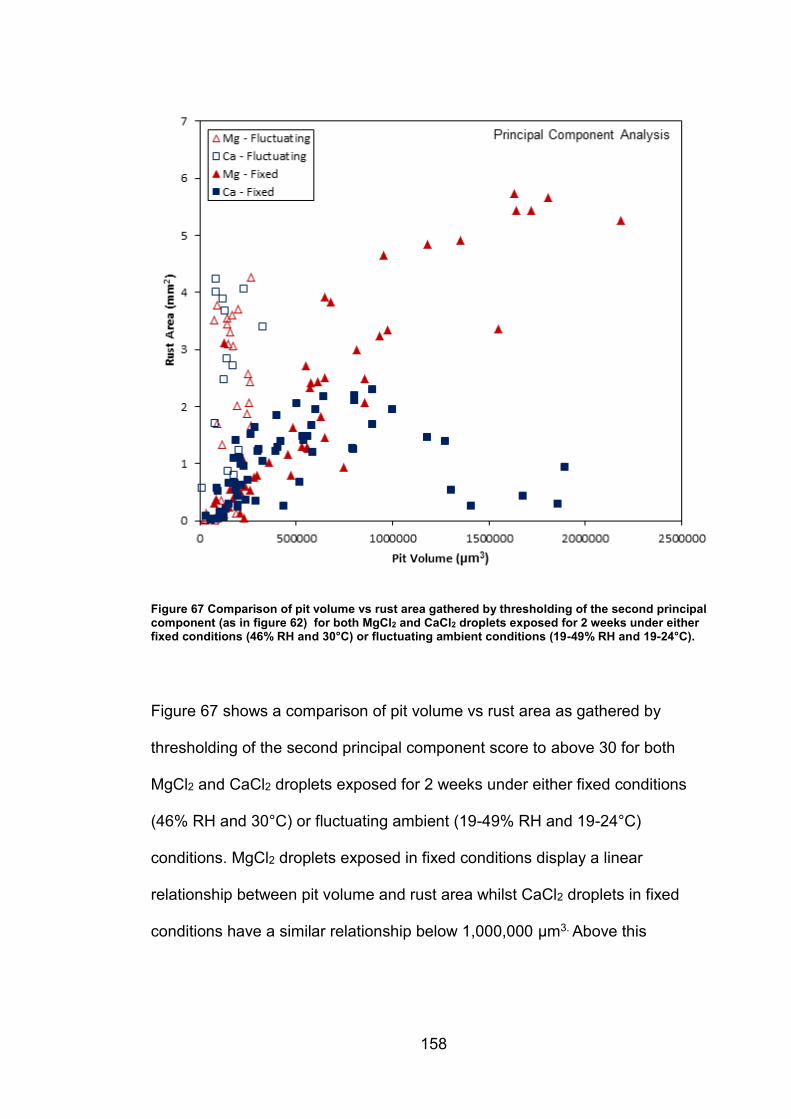
158

Figure 67 Comparison of pit volume vs rust area gathered by thresholding of the second principal component (as in figure 62) for both MgCl2 and CaCl2 droplets exposed for 2 weeks under either fixed conditions (46% RH and 30°C) or fluctuating ambient conditions (19-49% RH and 19-24°C).

Figure 67 shows a comparison of pit volume vs rust area as gathered by

thresholding of the second principal component score to above 30 for both

MgCl2 and CaCl2 droplets exposed for 2 weeks under either fixed conditions

(46% RH and 30°C) or fluctuating ambient (19-49% RH and 19-24°C)

conditions. MgCl2 droplets exposed in fixed conditions display a linear

relationship between pit volume and rust area whilst CaCl2 droplets in fixed

conditions have a similar relationship below 1,000,000 μm3. Above this

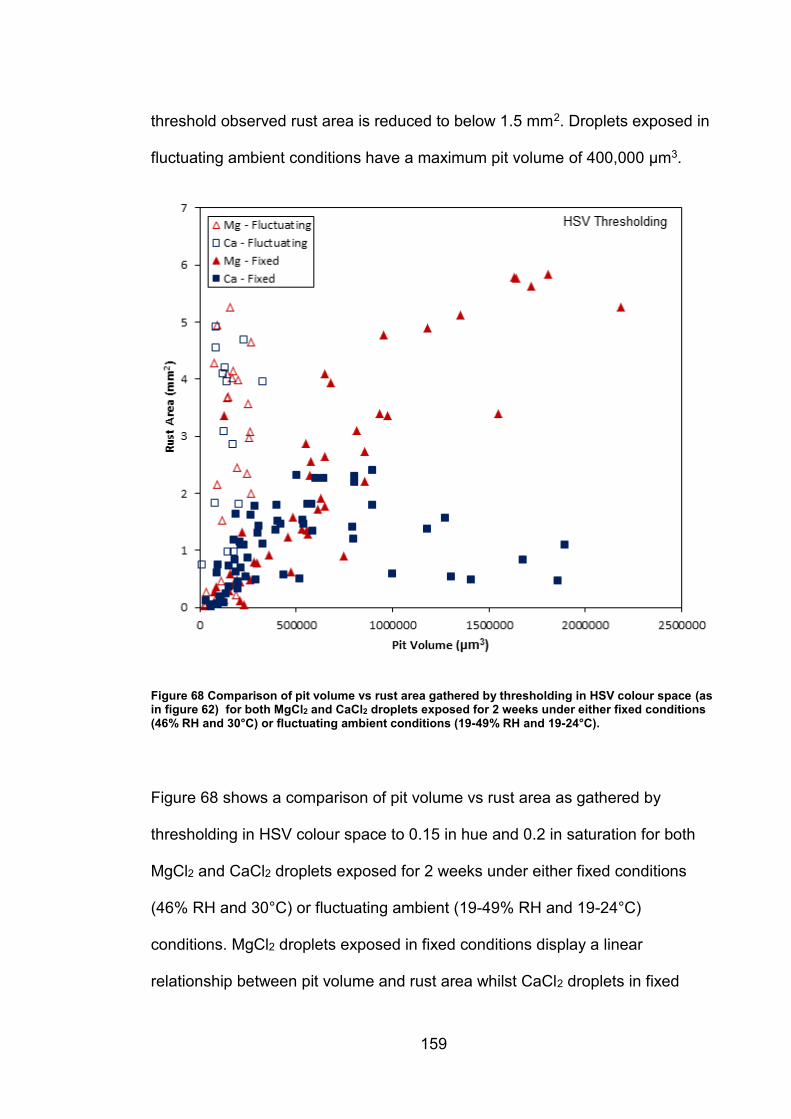
159

threshold observed rust area is reduced to below 1.5 mm2. Droplets exposed in

fluctuating ambient conditions have a maximum pit volume of 400,000 μm3.

Figure 68 Comparison of pit volume vs rust area gathered by thresholding in HSV colour space (as in figure 62) for both MgCl2 and CaCl2 droplets exposed for 2 weeks under either fixed conditions (46% RH and 30°C) or fluctuating ambient conditions (19-49% RH and 19-24°C).

Figure 68 shows a comparison of pit volume vs rust area as gathered by

thresholding in HSV colour space to 0.15 in hue and 0.2 in saturation for both

MgCl2 and CaCl2 droplets exposed for 2 weeks under either fixed conditions

(46% RH and 30°C) or fluctuating ambient (19-49% RH and 19-24°C)

conditions. MgCl2 droplets exposed in fixed conditions display a linear

relationship between pit volume and rust area whilst CaCl2 droplets in fixed

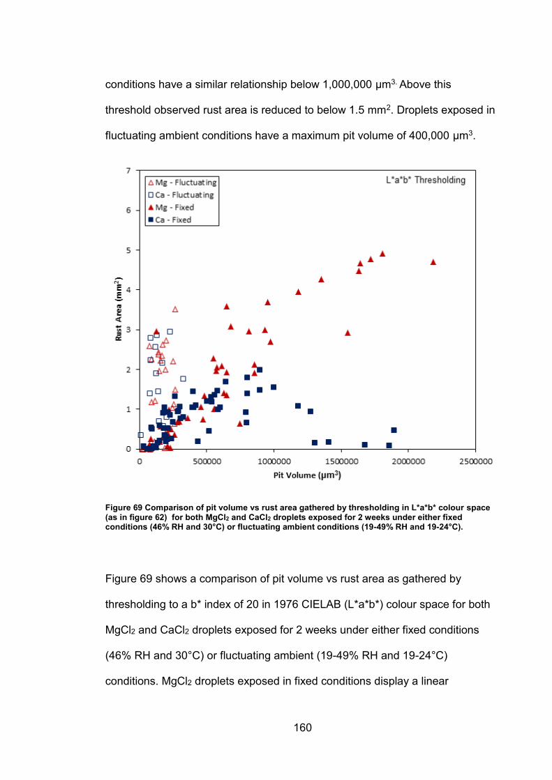
160

conditions have a similar relationship below 1,000,000 μm3. Above this

threshold observed rust area is reduced to below 1.5 mm2. Droplets exposed in

fluctuating ambient conditions have a maximum pit volume of 400,000 μm3.

Figure 69 Comparison of pit volume vs rust area gathered by thresholding in L*a*b* colour space (as in figure 62) for both MgCl2 and CaCl2 droplets exposed for 2 weeks under either fixed conditions (46% RH and 30°C) or fluctuating ambient conditions (19-49% RH and 19-24°C).

Figure 69 shows a comparison of pit volume vs rust area as gathered by

thresholding to a b* index of 20 in 1976 CIELAB (L*a*b*) colour space for both

MgCl2 and CaCl2 droplets exposed for 2 weeks under either fixed conditions

(46% RH and 30°C) or fluctuating ambient (19-49% RH and 19-24°C)

conditions. MgCl2 droplets exposed in fixed conditions display a linear

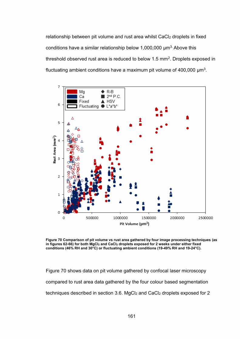
161

relationship between pit volume and rust area whilst CaCl2 droplets in fixed

conditions have a similar relationship below 1,000,000 μm3. Above this

threshold observed rust area is reduced to below 1.5 mm2. Droplets exposed in

fluctuating ambient conditions have a maximum pit volume of 400,000 μm3.

Figure 70 Comparison of pit volume vs rust area gathered by four image processing techniques (as in figures 62-66) for both MgCl2 and CaCl2 droplets exposed for 2 weeks under either fixed conditions (46% RH and 30°C) or fluctuating ambient conditions (19-49% RH and 19-24°C).

Figure 70 shows data on pit volume gathered by confocal laser microscopy

compared to rust area data gathered by the four colour based segmentation

techniques described in section 3.6. MgCl2 and CaCl2 droplets exposed for 2

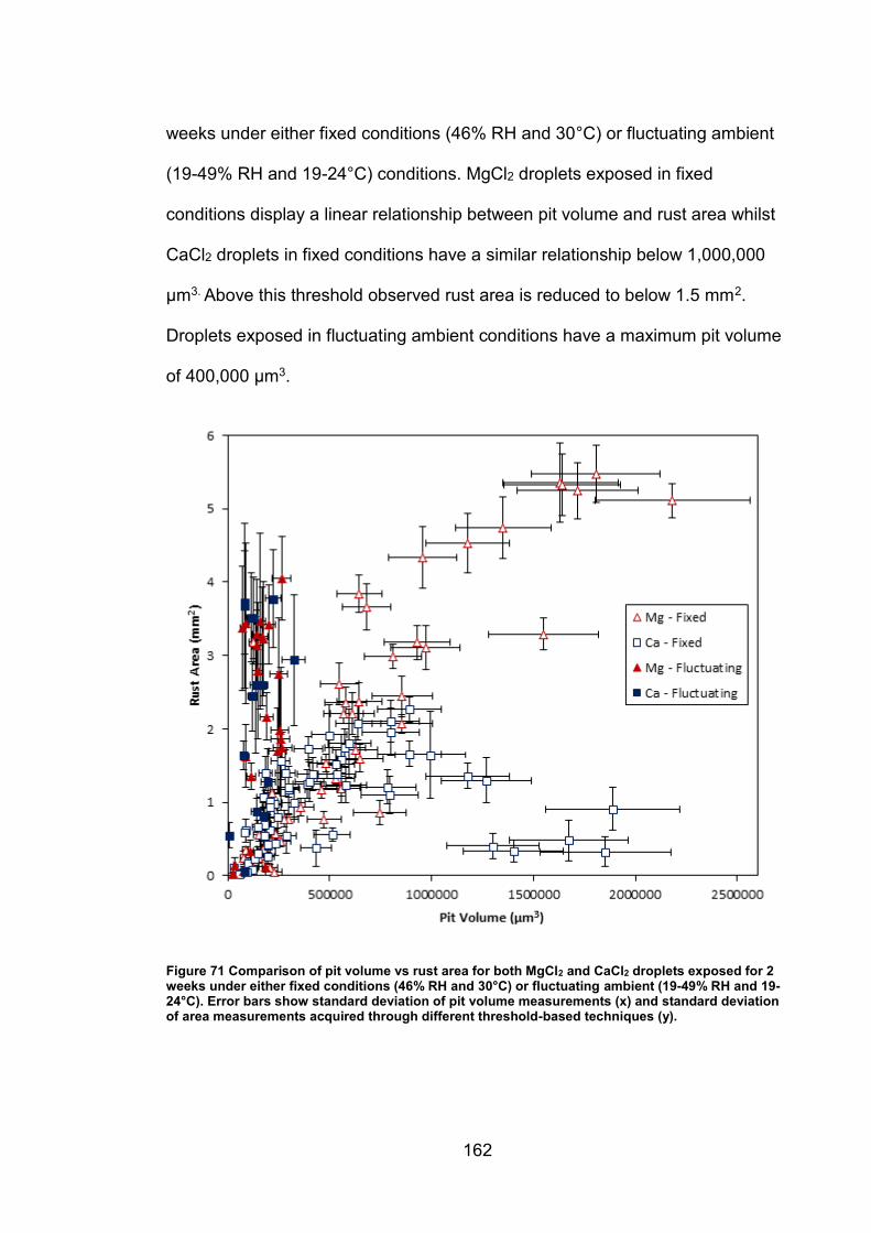
162

weeks under either fixed conditions (46% RH and 30°C) or fluctuating ambient

(19-49% RH and 19-24°C) conditions. MgCl2 droplets exposed in fixed

conditions display a linear relationship between pit volume and rust area whilst

CaCl2 droplets in fixed conditions have a similar relationship below 1,000,000

μm3. Above this threshold observed rust area is reduced to below 1.5 mm2.

Droplets exposed in fluctuating ambient conditions have a maximum pit volume

of 400,000 μm3.

Figure 71 Comparison of pit volume vs rust area for both MgCl2 and CaCl2 droplets exposed for 2 weeks under either fixed conditions (46% RH and 30°C) or fluctuating ambient (19-49% RH and 19-24°C). Error bars show standard deviation of pit volume measurements (x) and standard deviation of area measurements acquired through different threshold-based techniques (y).

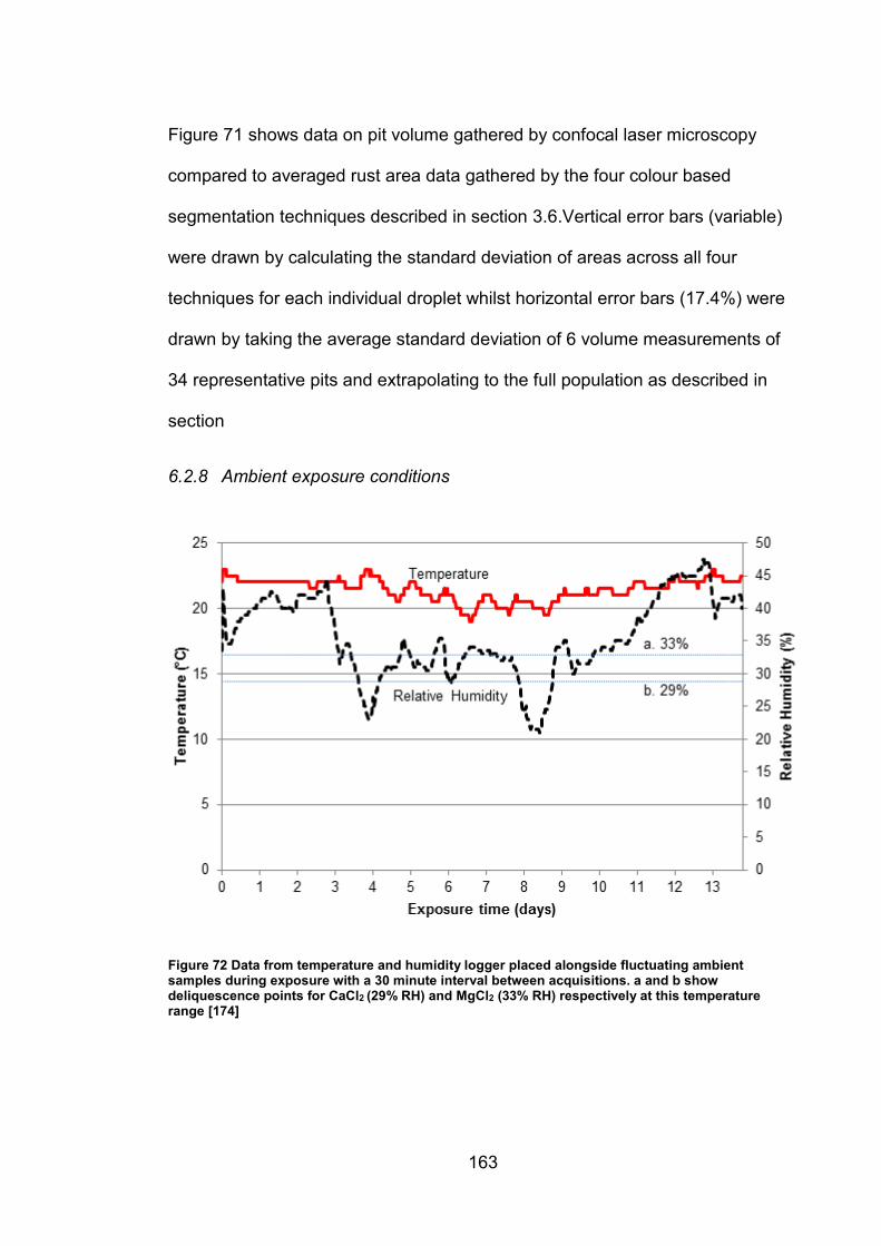
163

Figure 71 shows data on pit volume gathered by confocal laser microscopy

compared to averaged rust area data gathered by the four colour based

segmentation techniques described in section 3.6.Vertical error bars (variable)

were drawn by calculating the standard deviation of areas across all four

techniques for each individual droplet whilst horizontal error bars (17.4%) were

drawn by taking the average standard deviation of 6 volume measurements of

34 representative pits and extrapolating to the full population as described in

section

6.2.8 Ambient exposure conditions

Figure 72 Data from temperature and humidity logger placed alongside fluctuating ambient samples during exposure with a 30 minute interval between acquisitions. a and b show deliquescence points for CaCl2 (29% RH) and MgCl2 (33% RH) respectively at this temperature range [174]

164

Figure 72 shows the exposure conditions as recorded from a data logger placed

alongside the samples left open to fluctuating ambient conditions. The

temperature remains steady between 19°C and 23°C whilst the relative humidity

fluctuated between 20% and 43%. Deliquescence points of a. MgCl2·6H2O at

33% RH and b. CaCl2·6H2O at 29% RH are marked.[174]

6.3 Discussion

6.3.1 Pit volume measurements

A general increase in pit volume with chloride deposition density (CDD) was

observed for droplets exposed to fixed conditions, but this relationship was not

present for droplets in fluctuating conditions (Figure 57), where pit volumes

were consistently very low compared to those in fixed conditions.

It is well understood that pit morphology is heavily dependent on atmospheric

conditions via solution concentration[175, 176] and during this experiment the

droplets exposed to fluctuating ambient conditions spent significant amounts of

time at a lower relative humidity and temperature than the ones in fixed

conditions (Figure 72).

This would have a number of effects. Firstly a lower temperature would mean a

lower overall growth rate and a longer initiation time[63, 145] and secondly a

generally lower relative humidity would mean a more concentrated solution and

a thinner electrolyte layer, meaning a higher I-R drop limiting cathodic area. As

pit growth rate is cathodically controlled[8, 27, 55] this would manifest as lower

gross metal loss after a set time. This is likely to be in combination with a

change in morphology to a spiral or satellite mode rather than hemispherical, as

165

seen in Figure 54, Figure 55 and Figure 56. Significant volume of the pit could

be undercut and therefore unobserved by confocal microscopy.[64, 65] It’s also

worth noting that a larger number of small pits such as in a satellite pitting

regime might correspond to a lower risk of stress corrosion cracking for similar

total metal loss in a hemispherical pit[22, 177]. Additionally, preferential

dissolution of delta ferrite in 304L stainless steel could account for significant

‘lost’ volume as almost all of this growth could be undercut along the rolling

direction of the steel.[64] This makes volume assessment difficult without

vertical sectioning or sequential tomographic grinding of the sample, which

should be performed in future experiments. Finally, the relative humidity

dropped below the efflorescence point of the electrolyte salts twice during the

experiment, meaning that there was a risk that some or all of the droplets left in

fluctuating ambient conditions underwent wet-dry cycling. This drop was less

than a day in both cases however (Figure 72) and it has been previously

observed that this is not enough time for the occluded environment within the pit

to dry and repassivate.[44]

6.3.2 Rust area measurement

Rust area was assessed by image processing of colour photography through

four techniques: Red-Blue colour channel subtraction and thresholding (Figure 59),

Principal component analysis (PCA) followed by thresholding of the 2nd principal

component (Figure 60), thresholding of hue and saturation in HSV colour space

(Figure 61) and thresholding of b* (blue-yellow channel) in L*a*b* colour space

(Figure 62). Error! Reference source not found. shows the variation in area

measurement for each droplet in the dataset). Final thresholds for rust area

166

determination of the full dataset were determined by visual inspection of rust

area with respect to the extent segmented area by a particular threshold and

technique for a single droplet. i.e. The threshold which extracted the greatest

rust area without assigning any of the surrounding steel or salt was the one

used for rust area extraction for the full dataset.

Thresholds used for each technique were:

Residual intensity of 20 for R-B colour channel subtraction,

Score of 30 for principal component analysis

0.15 hue and 20 saturation for HSV

b* index of 20 for L*a*b*

After segmentation with appropriate thresholds (Error! Reference source not f

ound.), a general increase in rust area associated with chloride deposition

density was present for all four techniques on all droplets except CaCl2 droplets

exposed under fixed conditions. The low rust area gathered for CaCl2 droplets

with pits above 1,000,000 μm3 in fixed conditions was due to all techniques

requiring a colour gradient to be detected, which was minimal for these droplets

due to the dominant precipitation of a white corrosion product, determined as

green rust 1 in chapter 4. Figure 64 shows this in detail, the MgCl2 droplet’s red

colouration manifests as a clear difference in the distribution of red and blue

cannels, allowing the red area to be segmented while the CaCl2 droplets

distributions are equal, preventing segmentation.

All four segmentation techniques were able to separate rusty pixels from non-

rusty by colour. R-B colour channel subtraction gave consistently higher area

167

measurements than the mean of the 4 techniques, followed by HSV

thresholding, then 2nd P.C. and finally L*a*b* produced the lowest area

measurements. The average single droplet standard deviation from the mean

for all area measurement techniques was 24%, meaning results were

reasonably consistent.

6.3.3 Pit volume rust area comparison

Figure 66 - Figure 69 compare pit volume and rust area measured by each rust

area segmentation technique and Figure 70 shows all techniques in a single

plot for comparison. For all techniques, pit volume and rust area have a linear

relationship for droplets exposed to fixed conditions, excepting CaCl2 droplets

with a pit volume greater than 1,000,000 µm3. Above this volume threshold,

segmented rust area is much lower than would be expected from similar pits

under MgCl2 droplets.

Red-Blue colour channel subtraction (Figure 66) shows a generally higher area

of rust gathered, but a larger spread in the rust areas, while the principal

component analysis based technique (Figure 67) has a more consistent

relationship between pit volume and rust area as do the comparisons with HSV

(Figure 68) and L*a*b (Figure 69) techniques. It should be noted that the

principal component analysis based technique is unsupervised for the non-

thresholded portion of the process, meaning that the 2nd principal component

used for area allocation will show different pixels depending on the properties of

the data. i.e. if no rust is present in the image (red-blue variance axis), the

second principal component will show the next highest axis of variance in the

image. The other 3 techniques are all supervised for the whole process,

168

meaning that they require user input to set the thresholds which segment the

rust area. Under different lighting conditions or if a different camera is used,

these thresholds would need to be reassessed. As the 1976 CIELAB colour

space used for the L*a*b area measurement was designed to be device

independent, this need would be minimized for that technique.

Droplets exposed in fluctuating conditions have a similar spread of rust areas to

those in fixed, but due to their lower pit volumes, no correlation is present

between pit volume and rust area. Figure 71 shows the pit volume data against

averaged rust area data with error bars. The average standard deviation for the

rust area by the four techniques in Figure 54-Figure 57 was 24%, while the

average standard deviation of pit volume of a representative sample of pits was

17.4%. These are not large enough to significantly affect the confidence in the

trends in the data and no rust area segmentation technique proved decisively

more effective than any other.

Both pit volume and rust area were observed to increase with CDD for the

majority of droplets in fixed conditions (Figure 57, Error! Reference source not

found.), but only rust area was seen to increase for fluctuating ambient

conditions. This manifested as a linear relationship between pit volume and rust

area for MgCl2 droplets in fixed conditions and for CaCl2 droplets with pit

volumes of less than 1,000,000 µm3 (Figure 70, Figure 71), while no relationship

was present between pit volume and rust area for droplets exposed to

fluctuating ambient conditions.

169

In summary, rust area gathered by image processing of photography is a good

indicator of corrosion site presence, but preliminary attempts at quantification

are inconclusive due to unresolved questions with undercutting potentially

disrupting pit volume measurement and non-red corrosion product disrupting

area measurement. Future work should endeavour to improve reliability of

measurements by taking other corrosion products into account as well as total

rust volume or density into account instead of solely rust area. A tomographic

technique such as sequential grinding should also be utilized to measure pit

volume in order to resolve the question of unmeasured volume due to undercut

pit morphology.

6.4 Conclusions

The relationship between rust deposition area and pit volume on 304L stainless

steel after two weeks of exposure was assessed for fixed 46% relative humidity

and 30°C and ambient conditions which fluctuated between 20% - 46% RH and

19-23°C. Four colour-threshold based segmentation techniques were compared

for assessing rust area via colour photography and pit volume was measured

using confocal laser scanning microscopy.

1. Visible rust area increased with chloride deposition density for all

segmentation techniques, but no rust area segmentation technique

proved decisively more effective than any other.

2. In fixed conditions a linear relationship between pit volume and rust

areas was present for MgCl2 droplets and for all CaCl2 droplets with pits

of volume less than 1,000,000 µm3.

170

3. No relationship was observed between rust area and pit volume in

fluctuating conditions due to low observed pit volumes for a given rust

area.

4. CaCl2 droplets with pit volumes of greater than 1,000,000 μm3 generated

a band of green rust 1 which confounded rust area assessment by colour

analysis.

171

7. GENERAL DISCUSSION

Hyperspectral imaging and image processing of colour photography were

investigated with the aim of assessing their applicability to long term monitoring

of intermediate level waste containers. Corrosion product species that could be

expected to be present in waste stores were first identified using Raman

spectroscopic mapping for relevant salts and conditions. RGB colour and

hyperspectral images were then acquired and compared to Raman

spectroscopic mapping of a mature corrosion site in order to assess the viability

of different imaging techniques. Finally rust area was compared to pit volume in

order to investigate the relationship between visible surface rust and extent of

metal attack.

The corrosion products of 304L stainless steel were found to consist of the iron

oxide-hydroxide akaganeite (β-FeOOH), lepidocrocite (γ-FeOOH) and layered

double hydroxide (green rust) also present on some droplets. Akaganeite was

the majority phase present on most droplets, with a notable exception being

MgCl2 exposed to fluctuating ambient conditions which mainly consisted of

lepidocrocite. The ‘mature’ droplet utilised in chapter 5 had a mix of akaganeite,

lepidocrocite and green rust which made it viable for broad comparison between

HS imaging and colour photography.

When UV-VIS-NIR hyperspectral imaging was performed on a mature droplet

with a corrosion site containing all common corrosion products it was found that

specific phase identification was not possible with HS imaging i.e. only the

general presence of iron oxide-hydroxide could be distinguished from the

background steel. This was because the iron oxide-hydroxide spectra gathered

172

from droplet experiments have no significant features besides the broad band at

700-900 nm and as such the high spectral resolution (~ 1 nm) afforded by the

hyperspectral imaging apparatus is not utilised.

As a result, corrosion product detection can be performed by comparing just two

wavelength points – the maximum at 700-900 nm and the minimum at 500 nm.

High resolution colour photography was able to provide good rust area

assessment, with the red (~650 nm) and blue (~450 nm) colour channels of a

standard RGB colour camera providing an ‘off-the-shelf’ solution as sensors,

optics and software techniques designed for use with colour photography are

well understood and widely available. This did come at the cost of lower

contrast for corrosion detection, however, as the reflectivity of iron oxide-

hydroxide is lower at 650 nm (red) than 850 nm (near infra-red) as explored in

chapter 5.

Colour photography was used to assess rust area by way of this intensity

differential in chapter 6 and while there was no clear correlation drawn between

rust area and pit volume, rust was detected by using colour photography in

every droplet that pitted. It is worth noting that for CaCl2 droplets exposed to

fixed 46% RH for two weeks (Figure 34, Figure 64), the thick band of LDH-

green rust that was associated with large pits did not prevent detection of the

corrosion site entirely in any case.

A system might therefore be implemented whereby high resolution colour

photography provides fast, broad scale assessment of container surfaces to

highlight regions of interest for closer inspection and chemical analysis using

173

Raman spectroscopy, which would be able to better determine the chemical

composition of a particular region of interest.

7.1 Limitations

It should be noted that the investigations undertaken during the course of this

project had a number of potential limitations. Firstly, most droplets were

exposed for less than a month and therefore their corrosion products may not

be representative of those found in stores which could have been present for

years or even decades. However, comparing the distribution of corrosion

products of 30 μgcm-2 droplets present in Figure 37 (24 days exposure, fixed

46% RH and 30°C) and Figure 39 (14 days at fixed 46% RH and 30°C followed

by 42 months in fluctuating ambient conditions) suggests that the distribution

and species of corrosion product does not significantly change with additional

exposure time, only that species become better crystallised due to the lack

spectra with poor signal to noise and a single identifying peak at 710 cm-1. This

is further supported by Cornell and Schwertmann that suggest that significant

heating or pH change is required to undergo phase transformation[73]

Secondly, all experiments were performed on 304L stainless steel, when

containers will be made out of both 304L and 316L.[178] This is unlikely to

significantly affect the results as other alloying elements such as nickel and

chromium were not incorporated into corrosion products and so it’s not

expected that molybdenum would change the distribution or composition of

corrosion products. Boucherit et al discuss incorporation of molybdates into

goethite macrostructure, however [159] and so it is not out of the realm of

possibility that similar incorporation occurs with other iron oxide-hydroxides.

174

8. GENERAL CONCLUSIONS

Corrosion products of 304L stainless steel exposed to ILW stores relevant

atmospheric corrosion conditions were characterised using Raman

spectroscopic mapping. A hyperspectral imager was then assembled,

characterised and used to image a mature corrosion site in the 450-850 nm

wavelength interval, with iron oxide-hydroxide phase information being verified

by Raman spectroscopic mapping. Finally surface rust area assessed by colour

photography was compared to metal loss from pitting by volume gathered by

laser scanning confocal microscopy.

1. The major visible corrosion products were the iron oxide-hydroxides

akaganeite and lepidocrocite with a major secondary presence of layered

double hydroxide (green rust).

2. Colour based image segmentation was effective at detecting the

presence of pitting corrosion by the ring of iron oxide-hydroxide

deposited around the pit mouth

3. Iron oxide-hydroxide phase assignment on corrosion product from

droplet experiments was not possible using UV-VIS-NIR hyperspectral

imaging with a spectral range of 450 – 850 nm due to a lack of identifying

features in spectra acquired from precipitated rust.

4. Image segmentation of corrosion product species was more effective

when utilising the near infra-red (850 nm) rather than the red (650 nm),

producing up to 65% greater contrast with the blue (450 nm) due to iron

oxide-hydroxides’ reflectance being larger in this band.

175

5. The additional spectral resolution afforded by hyperspectral imaging is

not utilised due to the feature-poor UV-VIS-NIR spectrum of corrosion

products that precipitate in droplets and while there was the benefit of

additional image contrast from using hyperspectral imaging, the

additional complexity and acquisition time is significant. Colour

photography could instead be implemented as an off-the-shelf solution,

but would sacrifice the improved contrast of the NIR spectral region.

6. Visible surface rust was useful for indicating the presence of a corrosion

site, however no general correlation could be drawn between visible

surface rust and sub-surface attack in all circumstances. A relationship

was present for droplets exposed in fixed conditions, but there was no

correlation observed for those exposed to fluctuating ambient conditions.

176

9. FUTURE WORK

Tomographic techniques for improved pit volume measurement

A major confounding element in chapter 6 was the possibility of undercutting pit

morphology preventing accurate pit volume assessment, more accurate

methods of assessing pit volume such as vertical sectioning could be used in

the future.

The effects of relative humidity and temperature

The range of atmospheric conditions tested for was limited; a single RH and

temperature point for fixed conditions and poorly controlled fluctuating

conditions via ambient exposure. As it was found that corrosion product

morphology was significantly affected by atmospheric conditions, a larger range

of fixed conditions should be investigated, as well as a better controlled study

into what effects varying the atmospheric conditions have on the formation of

corrosion product.

The effects of salt accumulation over time

All droplet experiments were the result of a single deposition of salt, whereas

atmospheric corrosion in the real world involves the accumulation of salt over

time. This could have a significant effect on droplet formation and therefore on

final corrosion product distribution. Further investigation is needed into the

effects of droplet size and salt accumulation over time

Effects of other salt anions, cations as well as real-world compounds

All experiments were carried out using single salt depositions. Real world

conditions not only involve the simultaneous deposition of multiple different

177

chloride salts, but also multiple anions such as carbonates, nitrates and

sulphates. Combinatorial studies of these as well as standard mixes such as

concrete dust and ocean water would be useful for understanding the potential

effects of deposition mixtures on corrosion product formation.

Investigate corrosion product spectra in the SWIR region

No work was undertaken in the short wave infrared (SWIR) spectral region from

1000 nm to 2500nm. This is a region is made use of in industry and science and

while it is not as strongly diagnostic as the 400-1000 nm it has been reported to

be useful for assessment of hydration level of iron oxide-hydroxide[126]

Photography and hyperspectral imaging

A more detailed assessment comparing hyperspectral imaging to colour

photography is necessary as no investigation of false positive/negative

detection rate was performed and no possible confounding variables were

introduced such as non-corrosion related substances which might trigger

detection, such as paints, tape or dust.

178

10. REFERENCES

1. Frost R. The Road Not Taken. 1916. 2. Nuclear Decomissioning Authority, Geological Disposal: An overview of the generic Disposal System Safety Case. Radioactive Waste Management Limited. 2010. 3. Ramanaidou E, Wells M. Hyperspectral Imaging of Iron Ores. In: Broekmans MATM, editor. Proceedings of the 10th International Congress for Applied Mineralogy (ICAM): Springer Berlin Heidelberg; 2012. p. 575-80. 4. Sabins FF. Remote sensing for mineral exploration. Ore Geol Rev. 1999;14(3-4):157-83. 5. van der Meer FD, van der Werff HMA, van Ruitenbeek FJA, Hecker CA, Bakker WH, Noomen MF, et al. Multi- and hyperspectral geologic remote sensing: A review. Int J Appl Earth Obs Geoinf. 2012;14(1):112-28. 6. 2013 UK Radioactive Waste Inventory: Waste Quantities from all sources. 7. T.W. Hicks TDBaJMS, Galson Sciences Ltd, D.G. Bennett TL. Likelihood of Criticality: The Likelihood of Criticality Following Disposal of LLW/ILW/DNLEU. 2014. 8. Frankel GS. Pitting corrosion of metals. A review of the critical factors. Journal of the Electrochemical Society. 1998;145(8):2970-. 9. Harris C. Current Environmental Conditions Within Interim Stores and GDF Analogues. AMEC. 2012. 10. Authority ND. UK Radioactive Higher Activity Waste Storage Review, March 2009. 2009. 11. Harris C. A Survey of Current Environmental Conditions Within ILW Interim Stores and Potential GDF analogues. AMEC. 2015. 12. Drew N. Analysis of Chloride Deposition rates relevant to ILW stores. 2005. 13. P.A.H. Fennel NRS, M. Izzo, N.A. Turner. Characterisation of Environmental Conditions in an ILW Store. AMEC, 2012. 14. Fennell PAH. Characterisation of Environmental Conditions in an ILW store. AMEC. 2012. 15. R.J. Winsley NRS, B. Reddy, A.P. Rance, P.A.H. Fennell,. 4 metre Box Monitoring Programme - Final Report for the Period 2007-2010. Serco. 2011. 16. Padovani C, R.J. Winsley, N.R. Smart, P.A.H. Fennell, C Harris and K. Christie. Corrosion Control of Stainless Steels in Indoor Atmospheres - Practical Experience (Part 2). Corrosion. 2015. 17. Steel A. Product data sheet 304/304L Stainless steel. 2007. 18. Steel A. Product data sheet 316/316L stainless steel. 2007. 19. Bhadeshia. Steels - Microstructure and Properties. 3rd Ed. Oxford: Butterworth-Heinemann. 2006. 20. Olsson COA, Landolt D. Passive films on stainless steels—chemistry, structure and growth. Electrochim Acta. 2003;48(9):1093-104. 21. Marcus P, Moscatelli M. THE ROLE OF ALLOYED MOLYBDENUM IN THE DISSOLUTION AND THE PASSIVATION OF NICKEL-MOLYBDENUM ALLOYS IN THE PRESENCE OF ADSORBED SULFUR. Journal of the Electrochemical Society. 1989;136(6):1634-7. 22. Street SR, Mi N, Cook AJMC, Mohammed-Ali HB, Guo L, Rayment T, et al. Atmospheric pitting corrosion of 304L stainless steel: the role of highly concentrated chloride solutions. Faraday discussions. 2015;180:251-65. 23. Pourbaix MJN. Thermodynamique des solutions aqueuses diluées:

Représentation graphique du rôle du pH et du potentiel [PhD Thesis]. Delft: Delft Technical University. 1945.

179

24. Barry MaM, G. . Growth and Stability of Passive Films in Corrosion Mechanisms in Theory and Practice. CRC Press. 2002:189-216. 25. Asami K, Hashimoto K, Shimodaira S. XPS STUDY OF PASSIVITY OF A SERIES OF IRON-CHROMIUM ALLOYS IN SULFURIC-ACID. Corrosion Science. 1978;18(2):151-60. 26. Galvele JR. TRANSPORT PROCESSES AND MECHANISM OF PITTING OF METALS. Journal of the Electrochemical Society. 1976;123(4):464-74. 27. Newman RC. 2001 W.R. Whitney Award Lecture: Understanding the corrosion of stainless steel. Corrosion. 2002;58(3):292-. 28. Macdonald DD. THE POINT-DEFECT MODEL FOR THE PASSIVE STATE. Journal of the Electrochemical Society. 1992;139(12):3434-49. 29. Wranglen G. Pitting and sulphide inclusions in steel. Corrosion Science. 1974;14(5):331-49. 30. Jun J, Holguin K, Frankel GS. Pitting Corrosion of Very Clean Type 304 Stainless Steel. Corrosion. 2014;70(2):146-55. 31. Eklund GS. INITIATION OF PITTING AT SULFIDE INCLUSIONS IN STAINLESS-STEEL. Journal of the Electrochemical Society. 1974;121(4):467-73. 32. Baker MA, Castle JE. THE INITIATION OF PITTING CORROSION AT MNS INCLUSIONS. Corrosion Science. 1993;34(4):667-82. 33. Ke R, Alkire R. SURFACE-ANALYSIS OF CORROSION PITS INITIATED AT MNS INCLUSIONS IN 304 STAINLESS-STEEL. Journal of the Electrochemical Society. 1992;139(6):1573-80. 34. Ke RR, Alkire R. Initiation of corrosion pits at inclusions on 304 stainless steel. Journal of the Electrochemical Society. 1995;142(12):4056-62. 35. Wijesinghe T, Blackwood DJ. Real time pit initiation studies on stainless steels: The effect of sulphide inclusions. Corrosion Science. 2007;49(4):1755-64. 36. Galvele J. Transport processes in passivity breakdown—II. Full hydrolysis of the metal ions. Corrosion Science. 1981;21(8):551-79. 37. Williams DE, Kilburn MR, Cliff J, Waterhouse GIN. Composition changes around sulphide inclusions in stainless steels, and implications for the initiation of pitting corrosion. Corrosion Science. 2010;52(11):3702-16. 38. Isaacs HS. The localized breakdown and repair of passive surfaces during pitting. Corrosion Science. 1989;29(2):313-23. 39. Fontana M. Corrosion Engineering. New York: McGraw-Hill Book Company. 1986. 40. Isaacs HS. BEHAVIOR OF RESISTIVE LAYERS IN LOCALIZED CORROSION OF STAINLESS-STEEL. Journal of the Electrochemical Society. 1973;120(11):1456-62. 41. Beck TR, Alkire RC. OCCURRENCE OF SALT FILMS DURING INITIATION AND GROWTH OF CORROSION PITS. Journal of the Electrochemical Society. 1979;126(10):1662-6. 42. Alkire RC, Wong KP. THE CORROSION OF SINGLE PITS ON STAINLESS-STEEL IN ACIDIC CHLORIDE SOLUTION. Corrosion Science. 1988;28(4):411-&. 43. Laycock NJ, Newman RC. Localised dissolution kinetics, salt films and pitting potentials. Corrosion Science. 1997;39(10-11):1771-90. 44. Guo L. Atmospheric Localised corrosion of type 304 austenitic stainless steels [PHD thesis] University of Birmingham. 2016. 45. Tsutsumi Y, Nishikata A, Tsuru T. Pitting corrosion mechanism of Type 304 stainless steel under a droplet of chloride solutions. Corrosion Science. 2007;49(3):1394-407. 46. Evans UR. The Ferroxyl Indicator in Corrosion Research With special

180

Reference to the Controversey Regarding the Cause of Pitting. The Metal Industry. 1926;11. 47. Mi N, Ghahari M, Rayment T, Davenport AJ. Use of inkjet printing to deposit magnesium chloride salt patterns for investigation of atmospheric corrosion of 304 stainless steel. Corrosion Science. 2011;53(10):3114-21. 48. Wang YH, Wang W, Liu YY, Zhong L, Wang J. Study of localized corrosion of 304 stainless steel under chloride solution droplets using the wire beam electrode. Corrosion Science. 2011;53(9):2963-8. 49. Chen ZY, Kelly RG. Computational Modeling of Bounding Conditions for Pit Size on Stainless Steel in Atmospheric Environments. Journal of the Electrochemical Society. 2010;157(2):C69-C78. 50. Prosek T, Iversen A, Taxen C, Thierry D. Low-Temperature Stress Corrosion Cracking of Stainless Steels in the Atmosphere in the Presence of Chloride Deposits. Corrosion. 2009;65(2):105-17. 51. Tsutsumi Y, Nishikata A, Tsuru T. Initial stage of pitting corrosion of type 304 stainless steel under thin electrolyte layers containing chloride ions. Journal of the Electrochemical Society. 2005;152(9):B358-B63. 52. Hastuty S, Nishikata A, Tsuru T. Pitting corrosion of Type 430 stainless steel under chloride solution droplet. Corrosion Science. 2010;52(6):2035-43. 53. Chen A, Cao F, Liao X, Liu W, Zheng L, Zhang J, et al. Study of pitting corrosion on mild steel during wet–dry cycles by electrochemical noise analysis based on chaos theory. Corrosion Science. 2013;66:183-95. 54. Yadav AP, Nishikata A, Tsuru T. Electrochemical impedance study on galvanized steel corrosion under cyclic wet–dry conditions––influence of time of wetness. Corrosion Science. 2004;46(1):169-81. 55. Cruz RPV, Nishikata A, Tsuru T. Pitting corrosion mechanism of stainless steels under wet-dry exposure in chloride-containing environments. Corrosion Science. 1998;40(1):125-39. 56. Cruz RPV, Nishikata A, Tsuru T. AC impedance monitoring of pitting corrosion of stainless steel under a wet-dry cyclic condition in chloride-containing environment. Corrosion Science. 1996;38(8):1397-406. 57. Tran Van N, Tada E, Nishikata A. Pit Initiation and Repassivation of Stainless Steels Exposed to Cyclic Relative Humidity Changes. Journal of the Electrochemical Society. 2015;162(9):C419-C25. 58. Shi YY, Zhang Z, Su JX, Zhang JQ. EIS study on 2024-T3 aluminum alloy corrosion in simulated acid rain under cyclic wet-dry conditions. Mater Corros. 2005;56(10):701-6. 59. El-Mahdy G, Kim KB. AC impedance study on the atmospheric corrosion of aluminum under periodic wet-dry conditions. Electrochim Acta. 2004;49(12):1937-48. 60. Li CL, Ma YT, Li Y, Wang FH. EIS monitoring study of atmospheric corrosion under variable relative humidity. Corrosion Science. 2010;52(11):3677-86. 61. Schwenk W. THEORY OF STAINLESS STEEL PITTING. Corrosion. 1964;20(4):T129-&. 62. Maier B, Frankel GS. Pitting Corrosion of Bare Stainless Steel 304 under Chloride Solution Droplets. Journal of the Electrochemical Society. 2010;157(10):C302-C12. 63. Street SR. Atmospheric corrosion of austenitic stainless steels[PhD Thesis]. University of Birmingham. 2016. 64. Ali HBM. Atmospheric Pitting Corrosion of Stainless Steel [PhD Thesis]. University of Birmingham. 2016. 65. Davenport AJ, Guo L, Mi N, Mohammed-Ali H, Ghahari M, Street SR, et al. Mechanistic studies of atmospheric pitting corrosion of stainless steel for ILW containers. Corros Eng Sci Technol. 2014;49(6):514-20.

181

66. Albores-Silva OE. Atmospheric stress corrosion cracking and pitting of austenitic stainless steel: Newcastle University; 2011. 67. Albores-Silva OE, Charles EA, Padovani C. Effect of chloride deposition on stress corrosion cracking of 316L stainless steel used for intermediate level radioactive waste containers. Corros Eng Sci Technol. 2011;46(2):124-8. 68. Nurnberger U. STRESS-CORROSION CRACKING OF STAINLESS-STEEL STRUCTURAL COMPONENTS IN INDOOR SWIMMING POOLS. Stahl Und Eisen. 1990;110(6):141-8. 69. Faller M, Richner P. Material selection of safety-relevant components in indoor swimming pools. Mater Corros. 2003;54(5):331-8. 70. Gnanamoorthy JB. Stress corrosion cracking of unsensitized stainless steels in ambient-temperature coastal atmosphere1990. 63-5 p. 71. Christie K. The Examination and Reporting of Atmospheric Stress Corrosion Cracking Tests. NNC report C6125/TR/006. 2002(3). 72. Smart NRS. Literature Review of Atmospheric Stress Corrosion Cracking of Stainless Steels Report to NIREX. 2007. 73. R. M. Cornell US. The Iron Oxides: Structure, Properties, Reactions,Occurences and uses. 74. Misawa T, Hashimoto K, Shimodaira S. MECHANISM OF FORMATION OF IRON-OXIDE AND OXYHYDROXIDES IN AQUEOUS-SOLUTIONS AT ROOM-TEMPERATURE. Corrosion Science. 1974;14(2):131-49. 75. Scheck J, Lemke T, Gebauer D. The Role of Chloride Ions during the Formation of Akaganeite Revisited. Minerals. 2015;5(4):778-87. 76. Shebanova ON, Lazor P. Raman study of magnetite (Fe3O4): laser-induced thermal effects and oxidation. J Raman Spectrosc. 2003;34(11):845-52. 77. Hanesch M. Raman spectroscopy of iron oxides and (oxy)hydroxides at low laser power and possible applications in environmental magnetic studies. Geophys J Int. 2009;177(3):941-8. 78. Mazzetti L, Thistlethwaite PJ. Raman spectra and thermal transformations of ferrihydrite and schwertmannite. J Raman Spectrosc. 2002;33(2):104-11. 79. deFaria DLA, Silva SV, deOliveira MT. Raman microspectroscopy of some iron oxides and oxyhydroxides. J Raman Spectrosc. 1997;28(11):873-8. 80. Froment F, Tournie A, Colomban P. Raman identification of natural red to yellow pigments: ochre and iron-containing ores. J Raman Spectrosc. 2008;39(5):560-8. 81. Bellot-Gurlet L, Neff D, Reguer S, Monnier J, Saheb M, Dillmann P. Raman Studies of Corrosion Layers Formed on Archaeological Irons in Various Media. J Nano Res. 2009;8:147-56. 82. Monnier J, Bellot-Gurlet L, Baron D, Neff D, Guillot I, Dillmann P. A methodology for Raman structural quantification imaging and its application to iron indoor atmospheric corrosion products. J Raman Spectrosc. 2011;42(4):773-81. 83. Neff D, Bellot-Gurlet L, Dillmann P, Reguer S, Legrand L. Raman imaging of ancient rust scales on archaeological iron artefacts for long-term atmospheric corrosion mechanisms study. J Raman Spectrosc. 2006;37(10):1228-37. 84. Reguer S, Neff D, Bellot-Gurlet L, Dillmann P. Deterioration of iron archaeological artefacts: micro-Raman investigation on Cl-containing corrosion products. J Raman Spectrosc. 2007;38(4):389-97. 85. Haest M, Cudahy T, Laukamp C, Gregory S. Quantitative Mineralogy from Infrared Spectroscopic Data. II. Three-Dimensional Mineralogical Characterization of the Rocklea Channel Iron Deposit, Western Australia. Econ Geol. 2012;107(2):229-49. 86. Morris RV, Golden DC, Bell JF, Shelfer TD, Scheinost AC, Hinman NW, et al. Mineralogy, composition, and alteration of Mars Pathfinder rocks and soils: Evidence

182

from multispectral, elemental, and magnetic data on terrestrial analogue, SNC meteorite, and Pathfinder samples. J Geophys Res-Planets. 2000;105(E1):1757-817. 87. Morris RV, Lauer HV, Lawson CA, Gibson EK, Nace GA, Stewart C. SPECTRAL AND OTHER PHYSICOCHEMICAL PROPERTIES OF SUBMICRON POWDERS OF HEMATITE (ALPHA-FE2O3), MAGHEMITE (GAMMA-FE2O3), MAGNETITE (FE3O4), GOETHITE (ALPHA-FEOOH), AND LEPIDOCROCITE (GAMMA-FEOOH). Journal of Geophysical Research-Solid Earth and Planets. 1985;90(NB4):3126-44. 88. Sherman DM, Waite TD. ELECTRONIC-SPECTRA OF FE-3+ OXIDES AND OXIDE HYDROXIDES IN THE NEAR IR TO NEAR UV. Am Miner. 1985;70(11-12):1262-9. 89. Rancourt DG, Fortin D, Pichler T, Thibault PJ, Lamarche G, Morris RV, et al. Mineralogy of a natural As-rich hydrous ferric oxide coprecipitate formed by mixing of hydrothermal fluid and seawater: Implications regarding surface complexation and color banding in ferrihydrite deposits. Am Miner. 2001;86(7-8):834-51. 90. Li SX, George RD, Hihara LH. Corrosion analysis and characteristics of discarded military munitions in ocean waters. Corrosion Science. 2016;102:36-43. 91. Rout K, Mohapatra M, Anand S. 2-Line ferrihydrite: synthesis, characterization and its adsorption behaviour for removal of Pb(II), Cd(II), Cu(II) and Zn(II) from aqueous solutions. Dalton Trans. 2012;41(11):3302-12. 92. Dunnwald J, Otto A. AN INVESTIGATION OF PHASE-TRANSITIONS IN RUST LAYERS USING RAMAN-SPECTROSCOPY. Corrosion Science. 1989;29(9):1167-76. 93. Antony H, Legrand L, Marechal L, Perrin S, Dillmann P, Chausse A. Study of lepidocrocite gamma-FeOOH electrochemical reduction in neutral and slightly alkaline solutions at 25 degrees C. Electrochim Acta. 2005;51(4):745-53. 94. Antony H, Perrin S, Dillmann P, Legrand L, Chausse A. Electrochemical study of indoor atmospheric corrosion layers formed on ancient iron artefacts. Electrochim Acta. 2007;52(27):7754-9. 95. Dubois F, Mendibide C, Pagnier T, Perrard F, Duret C. Raman mapping of corrosion products formed onto spring steels during salt spray experiments. A correlation between the scale composition and the corrosion resistance. Corrosion Science. 2008;50(12):3401-9. 96. Legrand L, Sagon G, Lecomte S, Chausse A, Messina R. A Raman and infrared study of a new carbonate green rust obtained by electrochemical way. Corrosion Science. 2001;43(9):1739-49. 97. Genin JMR, Refait P, Bourrie G, Abdelmoula M, Trolard F. Structure and stability of the Fe(II)-Fe(III) green rust "fougerite" mineral and its potential for reducing pollutants in soil solutions. Applied Geochemistry. 2001;16(5):559-70. 98. Trolard F, Genin JMR, Abdelmoula M, Bourrie G, Humbert B, Herbillon A. Identification of a green rust mineral in a reductomorphic soil by Mossbauer and Raman spectroscopies. Geochimica Et Cosmochimica Acta. 1997;61(5):1107-11. 99. Luo H, Li XG, Dong CF, Xiao K. Degradation of austenite stainless steel by atmospheric exposure in tropical marine environment. Corros Eng Sci Technol. 2013;48(3):221-9. 100. Dong CF, Luo H, Xiao K, Ding Y, Li PH, Li XG. Electrochemical Behavior of 304 Stainless Steel in Marine Atmosphere and Its Simulated Solution. Anal Lett. 2013;46(1):142-55. 101. Dhaiveegan P, Elangovan N, Nishimura T, Rajendran N. Corrosion behavior of 316L and 304 stainless steels exposed to industrial-marine-urban environment: field study. RSC Adv. 2016;6(53):47314-24. 102. Tanaka S, Soc I, Control E. Non-destructive inspection of concrete structures using an electromagnetic wave radar. Tokyo: Soc Instrument Control Engineers Japan; 2004. 1493-7 p.

183

103. BDM Federal I. Corrosion Detection Technologies: A sector study. North American Technology and Industrial Base Organisation. 104. Agarwala VS, Reed PL, Ahmad S. Corrosion Detection and Monitoring - A Review. 2000/1/1/. NACE: NACE International. 105. N. Fuse TF. Evaluation of Applicability of Noncontact Analysis Methods to Detect Rust Regions in Coated Steel Plates. Transactions on terahertz science and technologu. 2012;2(2):242-9. 106. Rodriguez C, Biezma MV. Pitting corrosion detection in stainless steels using ultrasounds. Rev Metal. 2014;50(1):11. 107. V. Sharma TT. Techniques for detection of rusting od metals using image processing: a survey. Internation journal of emerging science and engineering. 2013;1(4). 108. Acosta MRG, Diaz JCV, Castro NS. An innovative image-processing model for rust detection using Perlin Noise to simulate oxide textures. Corrosion Science. 2014;88:141-51. 109. Ahuja SK, Shukla MK, Ravulakollu KK. Surface Corrosion Detection and Classification for Steel Alloy using Image Processing and Machine Learning. Helix. 2018;8(5):3822-7. 110. Medeiros FNS, Ramalho GLB, Bento MP, Medeiros LCL. On the Evaluation of Texture and Color Features for Nondestructive Corrosion Detection. Eurasip Journal on Advances in Signal Processing. 2010. 111. Eisberg RaR, R. Quantum Physics of Atoms, Molecules, Solids, Nuclei and Particles (Second Edition). 112. Wu. LVWaH-i. Biomedical optics: principles and imaging. John Wiley & Sons. 2012. 113. Blaschke T. Object based image analysis for remote sensing. ISPRS-J Photogramm Remote Sens. 2010;65(1):2-16. 114. Weng QH. Remote sensing of impervious surfaces in the urban areas: Requirements, methods, and trends. Remote Sens Environ. 2012;117:34-49. 115. Mulder VL, de Bruin S, Schaepman ME, Mayr TR. The use of remote sensing in soil and terrain mapping - A review. Geoderma. 2011;162(1-2):1-19. 116. Pal M, Mather PM. An assessment of the effectiveness of decision tree methods for land cover classification. Remote Sens Environ. 2003;86(4):554-65. 117. Mielke C, Boesche NK, Rogass C, Kaufmann H, Gauert C, de Wit M. Spaceborne Mine Waste Mineralogy Monitoring in South Africa, Applications for Modern Push-Broom Missions: Hyperion/OLI and EnMAP/Sentinel-2. Remote Sens. 2014;6(8):6790-816. 118. Bibring JP, Langevin Y, Gendrin A, Gondet B, Poulet F, Berthe M, et al. Mars surface diversity as revealed by the OMEGA/Mars Express observations. Science. 2005;307(5715):1576-81. 119. Goudge TA, Mustard JF, Head JW, Salvatore MR, Wiseman SM. Integrating CRISM and TES hyperspectral data to characterize a halloysite-bearing deposit in Kashira crater, Mars. Icarus. 2015;250:165-87. 120. Khelifi R, Adel M, Bourennane S. Segmentation of multispectral images based on band selection by including texture and mutual information. Biomed Signal Process Control. 2015;20:16-23. 121. Zabalza J, Ren JC, Zheng JB, Han JW, Zhao HM, Li ST, et al. Novel Two-Dimensional Singular Spectrum Analysis for Effective Feature Extraction and Data Classification in Hyperspectral Imaging. IEEE Trans Geosci Remote Sensing. 2015;53(8):4418-33. 122. Nansen C, Zhao GP, Dakin N, Zhao CH, Turner SR. Using hyperspectral imaging to determine germination of native Australian plant seeds. J Photochem Photobiol B-Biol. 2015;145:19-24.

184

123. Kamruzzaman M, ElMasry G, Sun DW, Allen P. Prediction of some quality attributes of lamb meat using near-infrared hyperspectral imaging and multivariate analysis. Anal Chim Acta. 2012;714:57-67. 124. Provoost J. Hyperspectral Imager Opens Options for Consumer, Medical and Industrial Uses. Photon Spect. 2015;49(4):46-50. 125. Bibring JP, Langevin Y, Mustard JF, Poulet F, Arvidson R, Gendrin A, et al. Global mineralogical and aqueous mars history derived from OMEGA/Mars express data. Science. 2006;312(5772):400-4. 126. Combe JP, Le Mouelic S, Sotin C, Gendrin A, Mustard JF, Le Deit L, et al. Analysis of OMEGA/Mars express data hyperspectral data using a Multiple-Endmember Linear Spectral Unmixing Model (MELSUM): Methodology and first results. Planet Space Sci. 2008;56(7):951-75. 127. Ducart DF, Silva AM, Bemfica Toledo CL, de Assis LM. Mapping iron oxides with Landsat-8/OLI and EO-1/Hyperion imagery from the Serra Norte iron deposits in the Carajas Mineral Province, Brazil. Brazilian Journal of Geology. 2016;46(3):331-49. 128. SharkD. By HSV_color_solid_cylinder.png: SharkDderivative work: SharkD Talk - HSV_color_solid_cylinder.png, CC BY-SA 3.0, https://commons.wikimedia.org/w/index.php?curid=9801673. 129. Jeffrey K. https://opentextbc.ca/graphicdesign/wp-content/uploads/sites/42/2015/04/Lab-colour-space.png, https://opentextbc.ca/graphicdesign/lab-colour-space/. License: Creative Commons 4.0 https://creativecommons.org/licenses/by/4.0/. 130. Consortium IC. Specification ICC.1:2004-10 (Profile version 4.2.0.0) [REVISION of ICC.1:2003-09]. Image technology colour management —

Architecture, profile format, and data structure. 2004. 131. Joblove GH, Greenberg D. Color spaces for computer graphics. SIGGRAPH Comput Graph. 1978;12(3):20-5. 132. E. Rehkugler G, A. Throop J. Apple Sorting with Machine Vision. Transactions of the ASAE.29(5):1388-97. 133. Cubero S, Aleixos N, Molto E, Gomez-Sanchis J, Blasco J. Advances in Machine Vision Applications for Automatic Inspection and Quality Evaluation of Fruits and Vegetables. Food and Bioprocess Technology. 2011;4(4):487-504. 134. Zhuang JJ, Luo SM, Hou CJ, Tang Y, He Y, Xue XY. Detection of orchard citrus fruits using a monocular machine vision-based method for automatic fruit picking applications. Computers and Electronics in Agriculture. 2018;152:64-73. 135. Itzhak D, Dinstein I, Zilberberg T. PITTING CORROSION EVALUATION BY COMPUTER IMAGE-PROCESSING. Corrosion Science. 1981;21(1):17-22. 136. Choi KY, Kim SS. Morphological analysis and classification of types of surface corrosion damage by digital image processing. Corrosion Science. 2005;47(1):1-15. 137. Valeti B, Pakzad S. Automated Detection of Corrosion Damage in Power Transmission Lattice Towers Using Image Processing. Soules JG, editor2017. 474-82 p. 138. Feliciano FF, Leta FR, Mainier FB. Texture digital analysis for corrosion monitoring. Corrosion Science. 2015;93:138-47. 139. Du Q, Fowler JE. Hyperspectral image compression using JPEG2000 and principal component analysis. Ieee Geoscience and Remote Sensing Letters. 2007;4(2):201-5. 140. Jia XP, Richards JA. Segmented principal components transformation for efficient hyperspectral remote-sensing image display and classification. IEEE Trans Geosci Remote Sensing. 1999;37(1):538-42.

185

141. Cheriyadat A, Bruce LM, Ieee, Ieee, Ieee. Why principal component analysis is not an appropriate feature extraction method for hyperspectral data. New York: Ieee; 2003. 3420-2 p. 142. Prasad S, Bruce LM. Limitations of Principal Components Analysis for Hyperspectral Target Recognition. Ieee Geoscience and Remote Sensing Letters. 2008;5(4):625-9. 143. Hancock PJB, Baddeley RJ, Smith LS. THE PRINCIPAL COMPONENTS OF NATURAL IMAGES. Netw-Comput Neural Syst. 1992;3(1):61-70. 144. Wang R, Nie FP, Yang XJ, Gao FF, Yao ML. Robust 2DPCA With Non-greedy l(1)-Norm Maximization for Image Analysis. IEEE T Cybern. 2015;45(5):1108-12. 145. Cook AJMC. The Atmospheric Corrosion of 304L and 316L stainless steels under conditions relevant to the itnerim storage of intermediate level nuclear waste [PhD Thesis]. University of Birmingham. 2017. 146. ASTM. E104-02(2007) "Standard Practice for maintaining constant relative humidity by means of aqueous solutions". 2007. 147. USAF MIL-STD-150A. US Defense Logistics Agency. 1951. 148. Matlab R2017b and Image Processing toolbox. Mathworks, Inc. ; 2017. 149. Ferreira MGS, Silva TME, Catarino A, Pankuch M, Melendres CA. ELECTROCHEMICAL AND LASER RAMAN-SPECTROSCOPY STUDIES OF STAINLESS-STEEL IN 0.15M NACL SOLUTION. Journal of the Electrochemical Society. 1992;139(11):3146-51. 150. Maslar JE, Hurst WS, Bowers WJ, Hendricks JH, Windsor ES. Alloy 600 Aqueous Corrosion at Elevated Temperatures and Pressures: An In Situ Raman Spectroscopic Investigation. Journal of the Electrochemical Society. 2009;156(3):C103-C13. 151. Ningshen S, Mudali UK, Ramya S, Raj B. Corrosion behaviour of AISI type 304L stainless steel in nitric acid media containing oxidizing species. Corrosion Science. 2011;53(1):64-70. 152. Kabekkodu DS. ICDD PDF-4+ 20xx (Database), available at: http://www.icdd.com/index.htm. 153. Glanvill S. ATMOSPHERIC CORROSION OF AA2024 IN OCEAN WATER ENVIRONMENTS [PHD THESIS]. University of Birmingham. 2018. 154. Belo MD, Walls M, Hakiki NE, Corset J, Picquenard E, Sagon G, et al. Composition, structure and properties of the oxide films formed on the stainless steel 316L in a primary type PWR environment. Corrosion Science. 1998;40(2-3):447-63. 155. Oblonsky LJ, Devine TM. Corrosion of carbon steels in CO2-saturated brine a surface enhanced Raman spectroscopic. Journal of the Electrochemical Society. 1997;144(4):1252-60. 156. Ramya S, Anita T, Shaikh H, Dayal RK. Laser Raman microscopic studies of passive films formed on type 316LN stainless steels during pitting in chloride solution. Corrosion Science. 2010;52(6):2114-21. 157. Shebanova ON, Lazor P. Raman spectroscopic study of magnetite (FeFe2O4): a new assignment for the vibrational spectrum. J Solid State Chem. 2003;174(2):424-30. 158. Thibeau RJ, Brown CW, Heidersbach RH. RAMAN-SPECTRA OF POSSIBLE CORROSION PRODUCTS OF IRON. Appl Spectrosc. 1978;32(6):532-5. 159. Boucherit N, Hugotlegoff A, Joiret S. INFLUENCE OF NI, MO, AND CR ON PITTING CORROSION OF STEELS STUDIED BY RAMAN-SPECTROSCOPY. Corrosion. 1992;48(7):569-79. 160. Socrates G. Infrared and Raman Characteristic Group Frequencies. Wiley. 2004. 161. Gu BH, Tio J, Wang W, Ku YK, Dai S. Raman spectroscopic detection for perchlorate at low concentrations. Appl Spectrosc. 2004;58(6):741-4.

186

162. Gomez RB. Hyperspectral imaging: a useful technology for transportation analysis. Opt Eng. 2002;41(9):2137-43. 163. Lagacherie P, Sneep AR, Gomez C, Bacha S, Coulouma G, Hamrouni MH, et al. Combining Vis-NIR hyperspectral imagery and legacy measured soil profiles to map subsurface soil properties in a Mediterranean area (Cap-Bon, Tunisia). Geoderma. 2013;209:168-76. 164. Padoan S, Klein, Aalderink, de Bruin. Quantitative Hyperspectral Imaging of historical documents: technique and applications. 9th international conference on NDT of Art, Jerusalem. 165. Gomez MA, Hendry MJ, Elouatik S, Essilfie-Dughan J, Paikaray S. Fe(II)((aq)) uptake of Mg(II)-Al(III)/Fe(III)-SO4/CO3 HTLCs under alkaline conditions: adsorption and solid state transformation mechanisms. RSC Adv. 2014;4(98):54973-88. 166. Folkman M, Pearlman J, Liao L, Jarecke P. EO-1/Hyperion hyperspectral imager design, development, characterization, and calibration. In: Smith WL, Yasuoka Y, editors. Hyperspectral Remote Sensing of the Land and Atmosphere. Proceedings of the Society of Photo-Optical Instrumentation Engineers (Spie). 4151. Bellingham: Spie-Int Soc Optical Engineering; 2001. p. 40-51. 167. Henrich V, Krauss G, Götze C, Sandow C. The IndexDatabase Bonn2011 [updated 2011]. Available from: https://www.indexdatabase.de/. 168. Tsai F, Philpot W. Derivative Analysis of Hyperspectral Data. Remote Sens Environ. 1998;66(1):41-51. 169. Leone AP, Sommer S. Multivariate analysis of laboratory spectra for the assessment of soil development and soil degradation in the southern Apennines (Italy). Remote Sens Environ. 2000;72(3):346-59. 170. Yang J, Zhang D, Frangi AF, Yang JY. Two-dimensional PCA: A new approach to appearance-based face representation and recognition. IEEE Trans Pattern Anal Mach Intell. 2004;26(1):131-7. 171. ASTM. G46 - 94 (2013) "Standard Guide for Examination and Evaluation of Pitting Corrosion". 2013. 172. Chen G, Qian S-E. Denoising of Hyperspectral Imagery Using Principal Component Analysis and Wavelet Shrinkage. IEEE Trans Geosci Remote Sensing. 2011;49(3):973-80. 173. Taguchi YH, Iwadate M, Umeyama H. Principal component analysis-based unsupervised feature extraction applied to in silico drug discovery for posttraumatic stress disorder-mediated heart disease. BMC Bioinformatics. 2015;16:26. 174. Lide D, and Cleveland. Handbook of Chemistry and Physics. 1994. 175. Street SR, Cook A, Mohammed-Ali HB, Rayment T, Davenport AJ. The Effect of Deposition Conditions on Atmospheric Pitting Corrosion Location Under Evans Droplets on Type 304L Stainless Steel. Corrosion. 2018;74(5):520-9. 176. Szklarska-Smialowska Z. Pitting Corrosion of Metals. Houston, Texas: National Association of Corrosion Engineers. 1986. 177. Jones RHaR, R.E. Stress-Corrosion Cracking Materials Performance and Evaluation. 1992. 178. King F. Container Materials for the Storage and Disposal of Nuclear Waste. Corrosion. 2013;69(10).

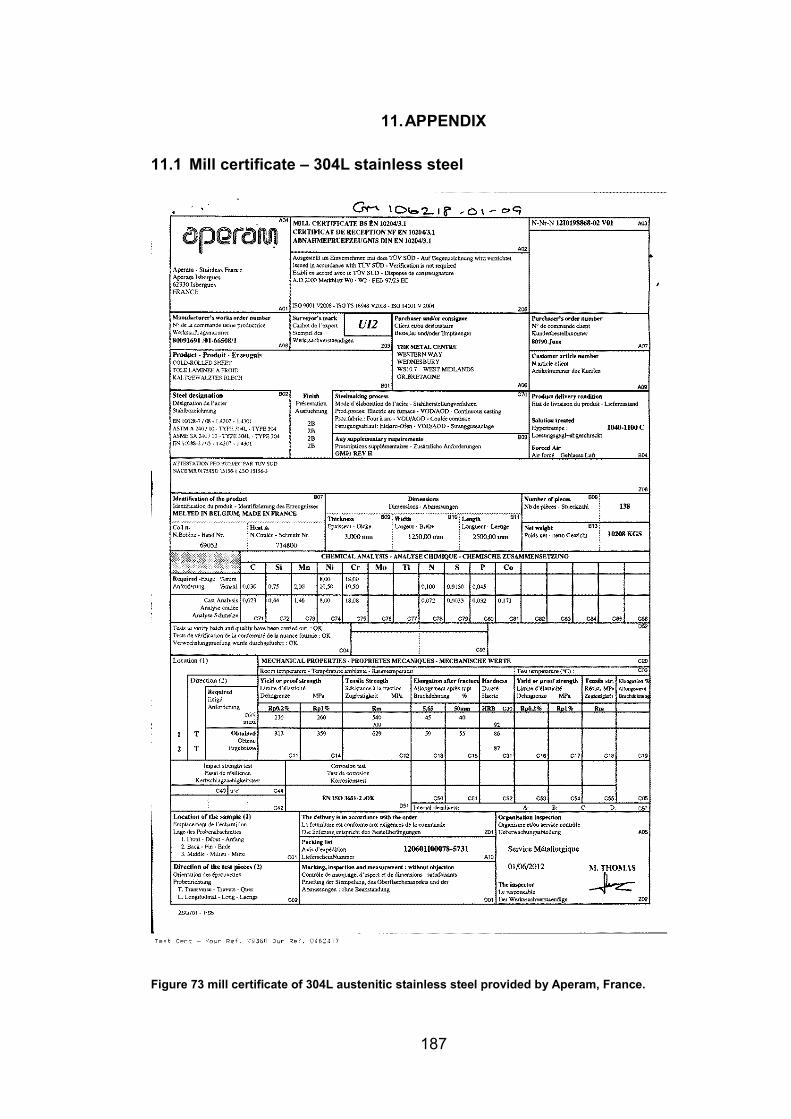
187

11. APPENDIX

11.1 Mill certificate – 304L stainless steel

Figure 73 mill certificate of 304L austenitic stainless steel provided by Aperam, France.

188

11.2 Powdered iron oxide standard synthesis

Powdered iron oxides were prepared by Dr. Rowena Fletcher-Wood using the

following procedures:

Akaganeite was precipitated from a solution consisting of 5.37 g of FeCl3.6H2O

(Sigma Aldrich 97%) dissolved in 200 ml deionised water, mixed in a

polypropylene flask and held at 70 °C in a preheated oven for 48 hours before

being immediately removed to cool to room temperature. An orange brown

grainy powder was produced that penetrated filter paper when filtered with a

Buchner funnel under suction filtration. To separate the solid from the liquid, the

sample was left to settle and water pipetted off to leave a dense suspension.

The remainder of the solution was left upon a warm oven for 5 days to dry,

before being scraped from the bottom of the flask.

Goethite was prepared by dissolving 25.24 g of KOH (Sigma Aldrich 90%) in

90 ml deionised water to get 5 M KOH solution which was subsequently

combined with 1 M Fe(NO3)3.9H2O (Aldrich 98+%) solution, itself prepared by

first dissolving 20.20 g of the solid in 50 ml deionised water. The solution was

diluted to 500 ml with deionised water and poured into a polypropylene flask,

sealed, then held at 70 °C in a preheated oven for 60 hours before turning off

the oven to allow the sample to cool to room temperature. The solution was

filtered with a Buchner funnel whilst still warm (~ 40 °C). The goethite

precipitate was a pale orange brown colour and crystals were shape flaky and

block-like.

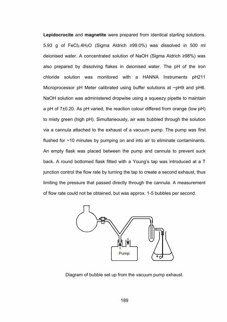
189

Lepidocrocite and magnetite were prepared from identical starting solutions.

5.93 g of FeCl2.4H2O (Sigma Aldrich ≥99.0%) was dissolved in 500 ml

deionised water. A concentrated solution of NaOH (Sigma Aldrich ≥98%) was

also prepared by dissolving flakes in deionised water. The pH of the iron

chloride solution was monitored with a HANNA Instruments pH211

Microprocessor pH Meter calibrated using buffer solutions at ~pH9 and pH6.

NaOH solution was administered dropwise using a squeezy pipette to maintain

a pH of 7±0.20. As pH varied, the reaction colour differed from orange (low pH)

to misty green (high pH). Simultaneously, air was bubbled through the solution

via a cannula attached to the exhaust of a vacuum pump. The pump was first

flushed for ~10 minutes by pumping on and into air to eliminate contaminants.

An empty flask was placed between the pump and cannula to prevent suck

back. A round bottomed flask fitted with a Young’s tap was introduced at a T

junction control the flow rate by turning the tap to create a second exhaust, thus

limiting the pressure that passed directly through the cannula. A measurement

of flow rate could not be obtained, but was approx. 1-5 bubbles per second.

Diagram of bubble set up from the vacuum pump exhaust.

190

Lepidocrocite was obtained after bubbling and holding the solution for 1 hour 20

minutes. At times exceeding 2 hours of bubbling, magnetite was obtained at

phase fractions of 98+%. At times ≤1 hour, a mixture of phases was obtained.

Maghemite was synthesised as a transformation product of magnetite,

prepared as described above with 2 hours of stirring and bubbling. The

magnetite sample was loaded into an open alumina boat and placed in a

preheated oven at 250 oC for 5 hours, before being removed to cool rapidly to

room temperature.

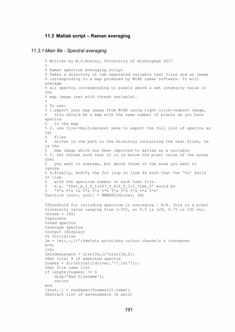
191

11.3 Matlab script – Raman averaging

11.3.1 Main file - Spectral averaging

% Written by W.G.Rowley, University of Birmingham 2017 % % Raman spectrum Averaging script % Takes a directory of tab seperated variable text files and an image % corresponding to a map produced by WiRE raman software. It will

average % all spectra corresponding to pixels above a set intensity value in

the % map image (set with thresh variable). % % To use: % 1.export your map image from WiRE using right click->export image, % this should be a bmp with the same number of pixels as you have

spectra % in the map % 2. use file->multidataset save to export the full list of spectra as

txt % files % dirvar is the path to the directory containing the text files, Im

is the % bmp image which has been imported to matlab as a variable % 3. Set thresh such that it is is below the pixel value of the areas

that % you want to average, but above those of the area you want to

ignore % 4.Finally, modify the for loop on line 46 such that the '%u' falls

in line % with the spectrum number on each text file. % e.g. 'Test_A_1_X_11243_Y_414_Z_312_Time_0' would be % '%*s %*s %u %*s %*s %*s %*s %*s %*s %*s %*s' function [xout, yout] = RMNAVG(dirvar, Im)

%Threshold for including spectrum in averaging | N.B. this is a pixel %intensity value ranging from 1-255, so 0.5 is 128, 0.75 is 191 etc. thresh = 100; %%process %read spectra %average spectra %output (display) %% Initialise Im = Im(:,:,1)';%delete pointless colour channels & transpose k=0; j=0; ImIndexLength = size(Im,1)*size(Im,2);

%Get total # of expected spectra fnames = dir(strcat([dirvar,'\*.txt']));

%Get file name list if length(fnames) == 0 disp('Bad Filename'); return end [xout,~] = readspec(fnames(1).name);

%Extract list of wavenumbers (x axis)

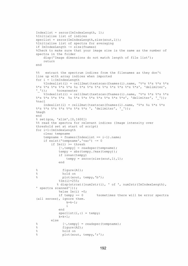
192

Indexlist = zeros(ImIndexLength, 1);

%Initialise list of indices speclist = zeros(ImIndexLength,size(xout,1));

%Initialise list of spectra for averaging if ImIndexLength ~= size(fnames)

%Check to make sure that your image size is the same as the number of

spectra in the folder disp('Image dimensions do not match length of file list'); return end

%% extract the spectrum indices from the filenames as they don't

line up with array indices when imported for i = 1:ImIndexLength %Indexlist(i) = cell2mat(textscan(fnames(i).name, '%*s %*s %*s %*s

%*s %*s %*s %*s %*s %u %*s %*s %*s %*s %*s %*s %*s %*s', 'delimiter',

'_')); %oceanwater %Indexlist(i) = cell2mat(textscan(fnames(i).name, '%*s %*s %*s %*s

%*s %*s %*s %*s %u %*s %*s %*s %*s %*s %*s %*s', 'delimiter', '_'));

%nacl Indexlist(i) = cell2mat(textscan(fnames(i).name, '%*s %u %*s %*s

%*s %*s %*s %*s %*s %*s %*s ', 'delimiter', '_'));

%magh end % set(gca, 'xlim',[0,1600]) %% read the spectra for relevant indices (Image intensity over

threshold set at start of script) for i=1:ImIndexLength clear tempname tempname = fnames(Indexlist == i-1).name; if exist('tempname','var') ~= 0 if Im(i) >= thresh [~,tempy] = readspec(tempname); tempy = abs(tempy./max(tempy)); if isnan(tempy) tempy = zeros(size(xout,1),1); end

% figure(A1); % hold on % plot(xout, tempy,'b'); %Im(i)=255; % disp(strcat([num2str(i), ' of ', num2str(ImIndexLength),

' spectra scanned'])); %else Im(i) =0; if tempy == 0 %sometimes there will be error spectra

(all zeroes), ignore them. k=k-1; i end speclist(i,:) = tempy; k=k+1; else % [~,tempy] = readspec(tempname); % figure(A2); % hold on % plot(xout, tempy,'r');

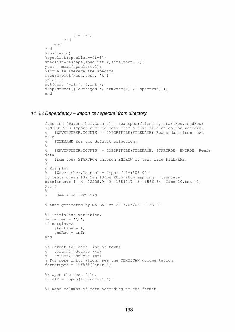
193

j = j+1; end end end %imshow(Im) %speclist(speclist==0)=[]; speclist=reshape(speclist,k,size(xout,1)); yout = mean(speclist,1);

%Actually average the spectra figure;plot(xout,yout, 'k')

%plot it set(gca, 'ylim',[0,inf]); disp(strcat(['Averaged ', num2str(k) ,' spectra'])); end

11.3.2 Dependency – import csv spectral from directory

function [Wavenumber,Counts] = readspec(filename, startRow, endRow) %IMPORTFILE Import numeric data from a text file as column vectors. % [WAVENUMBER,COUNTS] = IMPORTFILE(FILENAME) Reads data from text

file % FILENAME for the default selection. % % [WAVENUMBER,COUNTS] = IMPORTFILE(FILENAME, STARTROW, ENDROW) Reads

data % from rows STARTROW through ENDROW of text file FILENAME. % % Example: % [Wavenumber,Counts] = importfile('06-09-

16_test2_ocean_10s_2aq_100pw_28um-28um_mapping - truncate-

baselinesub_1__X_-22228.9__Y_-15589.7__Z_-6566.34__Time_20.txt',1,

981); % % See also TEXTSCAN.

% Auto-generated by MATLAB on 2017/05/03 10:33:27

%% Initialize variables. delimiter = '\t'; if nargin<=2 startRow = 1; endRow = inf; end

%% Format for each line of text: % column1: double (%f) % column2: double (%f) % For more information, see the TEXTSCAN documentation. formatSpec = '%f%f%[^\n\r]';

%% Open the text file. fileID = fopen(filename,'r');

%% Read columns of data according to the format.

194

% This call is based on the structure of the file used to generate

this % code. If an error occurs for a different file, try regenerating the

code % from the Import Tool. dataArray = textscan(fileID, formatSpec, endRow(1)-startRow(1)+1,

'Delimiter', delimiter, 'HeaderLines', startRow(1)-1, 'ReturnOnError',

false, 'EndOfLine', '\r\n'); for block=2:length(startRow) frewind(fileID); dataArrayBlock = textscan(fileID, formatSpec, endRow(block)-

startRow(block)+1, 'Delimiter', delimiter, 'HeaderLines',

startRow(block)-1, 'ReturnOnError', false, 'EndOfLine', '\r\n'); for col=1:length(dataArray) dataArray[80] = [dataArray[80];dataArrayBlock[80]]; end end

%% Close the text file. fclose(fileID);

%% Post processing for unimportable data. % No unimportable data rules were applied during the import, so no

post % processing code is included. To generate code which works for % unimportable data, select unimportable cells in a file and

regenerate the % script.

%% Allocate imported array to column variable names Wavenumber = dataArray{:, 1}; Counts = dataArray{:, 2};

11.4 Matlab scripts – Hyperspectral image processing

Scripts for importing hyperspectral images into matlab and plotting specific

spectra from a hyperspectral image

11.4.1 Principal component analysis

%function [eigenvectors, secpricom] = PCA_ndim(I) % this function takes a hyperspectral image, calculates the principle

components and % plots these as an image

close all X = []; % To make it faster we will re-size the image to be smaller %I = imresize(I,0.25);

% get size of image

195

[nr,nc,d]=size(I);

% Convert to a double variable I = double(I);

% extract the colours for i = 1:d In = I(:,:,i);

% instead of a matrix, we want a long list of pixel intensity In = reshape(In,nr*nc,1);

% This bit is where we calculate the PCA In = In-mean(In); In(In==Inf)=0; In(In==-Inf)=0; In(isnan(In))=0; X = [X, In]; end [U,S,V]=svd(cov(X));

eigenvectors= U'*X';

% and plot it! figure; for i = 1 : 5 subplot(1,5,i); imagesc(reshape(eigenvectors(i,:),nr,nc));axis equal;axis

tight;colormap gray; end firpricom =reshape(eigenvectors(1,:),nr,nc); secpricom = reshape(eigenvectors(2,:),nr,nc); thirpricom = reshape(eigenvectors(3,:),nr,nc); fourpricom = reshape(eigenvectors(4,:),nr,nc); fifpricom = reshape(eigenvectors(5,:),nr,nc); %subplot(1,3,3); %imagesc(reshape(eigenvectors(2,:)-(eigenvectors(1,:)./4),nr,nc));axis

equal;axis tight %end

11.5 Matlab scripts – Image processing

11.5.1 Acquire rust area by Red-Blue colour channel subtraction

% Takes an image; finds, labels pits by deposition area based on red-

blue % colour channel subtraction, boxes is optional %% I is a x*y*3 RGB image vector i.e. I = imread('IMAGE.NAME'); function output = colourfindrgb(I, boxes); if exist('boxes') == 0 boxes = false; end

196

%%classifying part %get size of image [nr,nc,d]=size(I);

% Convert to a double variable I = double(I);

% extract the colours IR = double(I(:,:,1)); IG = double(I(:,:,2)); IB = double(I(:,:,3));

thresh = IR-IB; %for R-B thresh(thresh < 30) = 0; %thresh of 30

%Dust and Assign labels to each region of connected components conncomps = bwconncomp(thresh); dust = cellfun(@numel,conncomps.PixelIdxList); thresh(cat(1, conncomps.PixelIdxList{dust<100}))=0;

almconncomp_im = bwdist(thresh) <= 50; L2 = labelmatrix(bwconncomp(almconncomp_im)); %Reduce areas to their original sizes L2(~thresh) = 255;

%Extract Areas and Centroids and plot. We also have the option to

colour %the plot based on label area s = regionprops(L2, 'Area', 'Centroid', 'Extrema', 'BoundingBox'); figure; imshow(L2); %imshow(label2rgb(L2, 'jet', 'w','shuffle')); % colour

%clean up output image %L2(L2~=255) = 1;

%Initialise output variables Area = zeros(1,length(s)); Centroid = zeros(2,length(s)); Extrema = zeros(8,2,length(s)); BB = zeros(4, length(s));

%Populate output variables from struct and amend plot with desired %features. hold on; for i = 1:(length(s)-1); if s(i).Area > 100 %%&& s(i).Area < 1000000 Area(:,i) = s(i).Area; Centroid(:,i) = s(i).Centroid; Extrema(:,:,i) = s(i).Extrema; BB(:,i) = s(i).BoundingBox; if boxes == true %plot(Centroid(1,i),Centroid(2,i),'b*');

%Mark the centroid of each region %plot(Extrema(:,1,i), Extrema(:,2,i), 'r+');

%Mark the extremeties of each region

197

rectangle('Position',BB(:,i));

%Draw a square around each region %viscircles(rot90(Centroid(:,i)),(Centroid(2,i)-BB(2,i)));

%Draw a circle around each region end end end %%output and close output = struct('Areas', Area, 'Centroid', Centroid, 'Extrema',

Extrema, 'BoundingBox', BB, 'Im', L2); hold off end

11.5.2 Acquire rust area by principal component analysis

% Takes an image; finds, labels pits by deposition area based on

principle % component analysis, boxes is optional %% I is a x*y*3 RGB image vector i.e. I = imread('IMAGE.NAME'); function output = pitfind(I, boxes); if exist('boxes') == 0 boxes = false; end %%PCA portion %get size of image [nr,nc,d]=size(I);

% Convert to a double variable I = double(I);

% extract the colours IR = I(:,:,1); IG = I(:,:,2); IB = I(:,:,3);

% instead of a matrix, we want a long list of pixel intensity IR = reshape(IR,nr*nc,1); IG = reshape(IG,nr*nc,1); IB = reshape(IB,nr*nc,1);

% This bit is where we calculate the PCA; %we first centre the data by subtracting the mean of each channel from

each channel IR = IR-mean(IR); IG = IG-mean(IG); IB = IB-mean(IB);

%These then get put in a single matrix X = [IR, IG, IB];

%Single value decomposition of the covariance matrix is performed [U,S,V]=svd(cov(X));

%the eigenvectors are then extracted by multiplying the transpose of

the

198

%unitary matrix U by the transpose of X. eigenvectors= U'*X';

%the second principle component (second channel) is extracted from the %eigenvector and reshaped back into the original resolution of the

image %(nr, nc) secpricom = reshape(eigenvectors(2,:),nr,nc);

%clearvars -except secpricom I

%%Regionfinding portion %Thresholding, all pixels of less than 50 intensity are set to zero thresh = secpricom; thresh(thresh < 20) = 0;

%Dust and Assign labels to each region of connected components conncomps = bwconncomp(thresh); dust = cellfun(@numel,conncomps.PixelIdxList); thresh(cat(1, conncomps.PixelIdxList{dust<100}))=0;

almconncomp_im = bwdist(thresh) <= 2; L2 = labelmatrix(bwconncomp(almconncomp_im)); %Reduce areas to their original sizes L2(~thresh) = 255;

%Extract Areas and Centroids and plot. We also have the option to

colour %the plot based on label area s = regionprops(L2, 'Area', 'Centroid', 'Extrema', 'BoundingBox'); figure; imshow(L2); %imshow(label2rgb(L2, 'jet', 'w','shuffle')); %colour

%clean up output image %L2(L2~=255) = 1;

%Initialise output variables Area = zeros(1,length(s)); Centroid = zeros(2,length(s)); Extrema = zeros(8,2,length(s)); BB = zeros(4, length(s));

%Populate output variables from struct and amend plot with desired %features. hold on; for i = 1:(length(s)-1); if s(i).Area > 100 %%&& s(i).Area < 1000000 Area(:,i) = s(i).Area; Centroid(:,i) = s(i).Centroid; Extrema(:,:,i) = s(i).Extrema; BB(:,i) = s(i).BoundingBox; if boxes == true %plot(Centroid(1,i),Centroid(2,i),'b*');

%Mark the centroid of each region

199

%plot(Extrema(:,1,i), Extrema(:,2,i), 'r+');

%Mark the extremeties of each region rectangle('Position',BB(:,i));

%Draw a square around each region %viscircles(rot90(Centroid(:,i)),(Centroid(2,i)-BB(2,i)));

%Draw a circle around each region end end end %%output and close output = struct('Areas', Area, 'Centroid', Centroid, 'Extrema',

Extrema, 'BoundingBox', BB, 'Im', L2); hold off end

11.5.3 Acquire rust area by HSV thresholding

% Takes an image; finds, labels pits by deposition area based on HSV

thresholding, boxes is optional %% I is a x*y*3 RGB image vector i.e. I = imread('IMAGE.NAME'); function output = colourfindhsv(I, boxes); if exist('boxes') == 0 boxes = false; end %%classifying part %get size of image

[nr,nc,d]=size(I);

% Convert to hsv I = rgb2hsv(I);

% extract the variables Ih = I(:,:,1); Is = I(:,:,2); Iv = I(:,:,3);

thresh = Is; %doing everything via the saturation

channel thresh(Ih > 0.15) = 0; %eliminate H that's not red thresh(Is < 0.2) = 0; %threshold of 0.2S

%Dust and Assign labels to each region of connected components conncomps = bwconncomp(thresh); dust = cellfun(@numel,conncomps.PixelIdxList); thresh(cat(1, conncomps.PixelIdxList{dust<100}))=0;

almconncomp_im = bwdist(thresh) <= 50; L2 = labelmatrix(bwconncomp(almconncomp_im)); %Reduce areas to their original sizes L2(~thresh) = 255;

200

%Extract Areas and Centroids and plot. We also have the option to

colour %the plot based on label area s = regionprops(L2, 'Area', 'Centroid', 'Extrema', 'BoundingBox'); figure; imshow(L2); %imshow(label2rgb(L2, 'jet', 'w','shuffle')); %colour %clean up output image %L2(L2~=255) = 1;

%Initialise output variables Area = zeros(1,length(s)); Centroid = zeros(2,length(s)); Extrema = zeros(8,2,length(s)); BB = zeros(4, length(s));

%Populate output variables from struct and amend plot with desired %features. hold on; for i = 1:(length(s)-1); if s(i).Area > 100 %%&& s(i).Area < 1000000 Area(:,i) = s(i).Area; Centroid(:,i) = s(i).Centroid; Extrema(:,:,i) = s(i).Extrema; BB(:,i) = s(i).BoundingBox; if boxes == true %plot(Centroid(1,i),Centroid(2,i),'b*');

%Mark the centroid of each region %plot(Extrema(:,1,i), Extrema(:,2,i), 'r+');

%Mark the extremeties of each region rectangle('Position',BB(:,i));

%Draw a square around each region %viscircles(rot90(Centroid(:,i)),(Centroid(2,i)-BB(2,i)));

%Draw a circle around each region end end end %%output and close output = struct('Areas', Area, 'Centroid', Centroid, 'Extrema',

Extrema, 'BoundingBox', BB, 'Im', L2); hold off end

11.5.4 Rust area analysis by L*a*b* thresholding

% Takes an image; finds, labels pits by deposition area based on

L*a*b* thresholding, boxes is optional %% I is a x*y*3 RGB image vector i.e. I = imread('IMAGE.NAME'); function output = colourfindlab(I, boxes); if exist('boxes') == 0 boxes = false;

201

end %%classifying part %get size of image

[nr,nc,d]=size(I);

% Convert to lab I = rgb2lab(I);

% extract the variables Il = I(:,:,1); Ia = I(:,:,2); Ib = I(:,:,3);

thresh = Ib; %doing everything via the b* channel thresh(thresh < 20) = 0;

%Dust and Assign labels to each region of connected components conncomps = bwconncomp(thresh); dust = cellfun(@numel,conncomps.PixelIdxList); thresh(cat(1, conncomps.PixelIdxList{dust<100}))=0;

almconncomp_im = bwdist(thresh) <= 50; L2 = labelmatrix(bwconncomp(almconncomp_im)); %Reduce areas to their original sizes L2(~thresh) = 255;

%Extract Areas and Centroids and plot. We also have the option to

colour %the plot based on label area s = regionprops(L2, 'Area', 'Centroid', 'Extrema', 'BoundingBox'); figure; imshow(L2); %imshow(label2rgb(L2, 'jet', 'w','shuffle')); % colour

%clean up output image %L2(L2~=255) = 1;

%Initialise output variables Area = zeros(1,length(s)); Centroid = zeros(2,length(s)); Extrema = zeros(8,2,length(s)); BB = zeros(4, length(s));

%Populate output variables from struct and amend plot with desired %features. hold on; for i = 1:(length(s)-1); if s(i).Area > 100 %%&& s(i).Area < 1000000 Area(:,i) = s(i).Area; Centroid(:,i) = s(i).Centroid; Extrema(:,:,i) = s(i).Extrema; BB(:,i) = s(i).BoundingBox; if boxes == true %plot(Centroid(1,i),Centroid(2,i),'b*');

%Mark the centroid of each region

202

%plot(Extrema(:,1,i), Extrema(:,2,i), 'r+');

%Mark the extremeties of each region rectangle('Position',BB(:,i));

%Draw a square around each region %viscircles(rot90(Centroid(:,i)),(Centroid(2,i)-BB(2,i)));

%Draw a circle around each region end end end %%output and close output = struct('Areas', Area, 'Centroid', Centroid, 'Extrema',

Extrema, 'BoundingBox', BB, 'Im', L2); hold off end

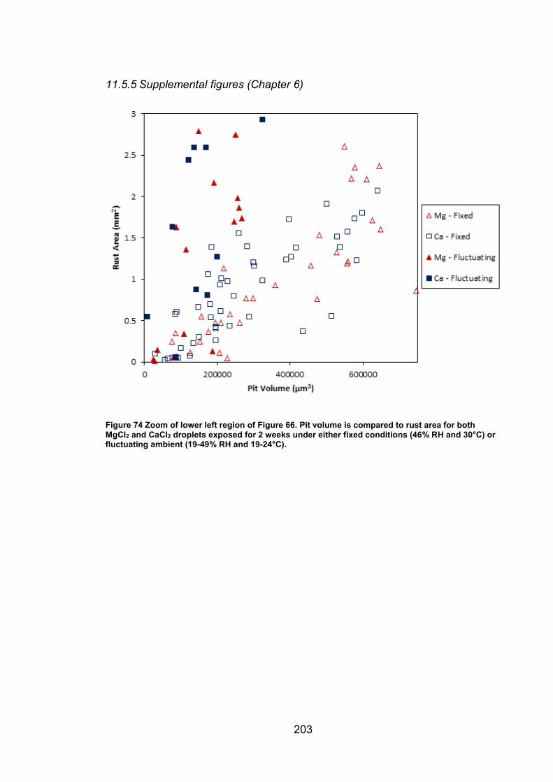
203

11.5.5 Supplemental figures (Chapter 6)

Figure 74 Zoom of lower left region of Figure 66. Pit volume is compared to rust area for both MgCl2 and CaCl2 droplets exposed for 2 weeks under either fixed conditions (46% RH and 30°C) or fluctuating ambient (19-49% RH and 19-24°C).

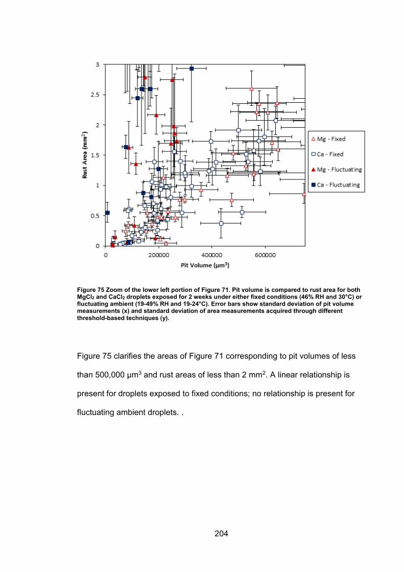
204

Figure 75 Zoom of the lower left portion of Figure 71. Pit volume is compared to rust area for both MgCl2 and CaCl2 droplets exposed for 2 weeks under either fixed conditions (46% RH and 30°C) or fluctuating ambient (19-49% RH and 19-24°C). Error bars show standard deviation of pit volume measurements (x) and standard deviation of area measurements acquired through different threshold-based techniques (y).

Figure 75 clarifies the areas of Figure 71 corresponding to pit volumes of less

than 500,000 µm3 and rust areas of less than 2 mm2. A linear relationship is

present for droplets exposed to fixed conditions; no relationship is present for

fluctuating ambient droplets. .

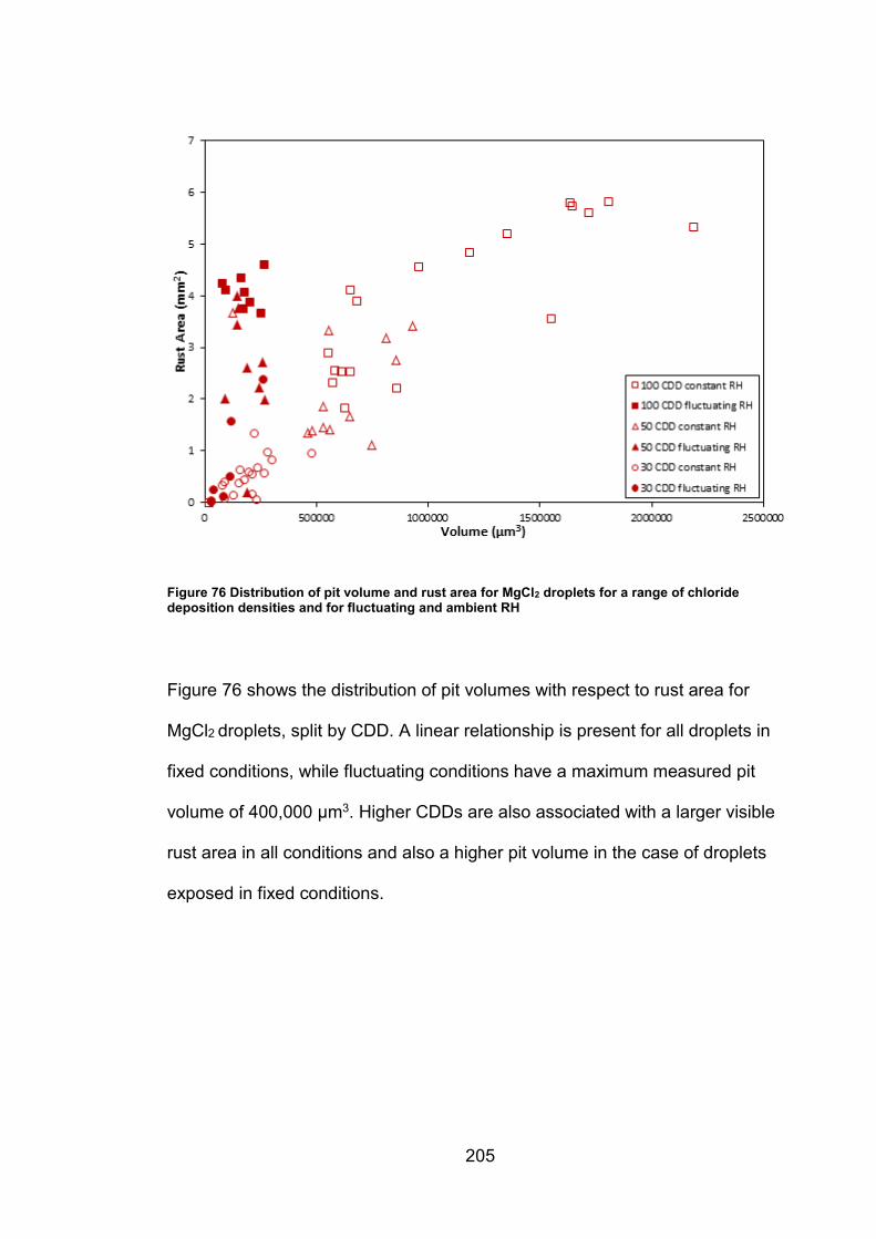
205

Figure 76 Distribution of pit volume and rust area for MgCl2 droplets for a range of chloride deposition densities and for fluctuating and ambient RH

Figure 76 shows the distribution of pit volumes with respect to rust area for

MgCl2 droplets, split by CDD. A linear relationship is present for all droplets in

fixed conditions, while fluctuating conditions have a maximum measured pit

volume of 400,000 µm3. Higher CDDs are also associated with a larger visible

rust area in all conditions and also a higher pit volume in the case of droplets

exposed in fixed conditions.

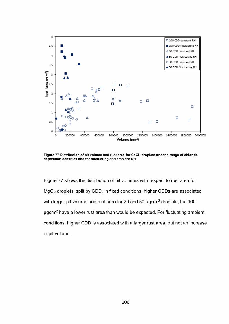
206

Figure 77 Distribution of pit volume and rust area for CaCl2 droplets under a range of chloride deposition densities and for fluctuating and ambient RH

Figure 77 shows the distribution of pit volumes with respect to rust area for

MgCl2 droplets, split by CDD. In fixed conditions, higher CDDs are associated

with larger pit volume and rust area for 20 and 50 µgcm-2 droplets, but 100

µgcm-2 have a lower rust area than would be expected. For fluctuating ambient

conditions, higher CDD is associated with a larger rust area, but not an increase

in pit volume.

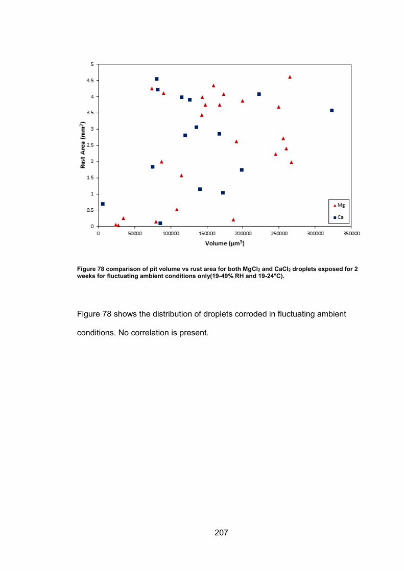
207

Figure 78 comparison of pit volume vs rust area for both MgCl2 and CaCl2 droplets exposed for 2 weeks for fluctuating ambient conditions only(19-49% RH and 19-24°C).

Figure 78 shows the distribution of droplets corroded in fluctuating ambient

conditions. No correlation is present.