universit a degli studi di napoli federico ii the density ... · the density valued data analysis...
TRANSCRIPT
Universita degli Studi di NapoliFederico II
The Density Valued Data Analysis in a TemporalFramework:
The Data Model Approach
Carlo Drago
Ph.D DissertationStatistics
XXIV Cycle

The Density Valued Data Analysis in a TemporalFramework
The Data Model Approach
Napoli, 30 November 2011
III


”Non se ne andra piu” gli dico.”Non se ne andra piu?””Nulla se ne andra piu.”
. . . ”Perche?” egli dice ”Che accade?”
” . . . Nessuna cosa ora e sola.”
”Sarebbe ogni cosa anche tutto il resto?”
” Precisamente. E dov’e una cosa, e anche tutto il resto . . . ”
. . . Viene l’infanzia lo stesso; viene la terra intesa come fu con fioribianchi ch’erano di capperi e sembravano farfalle; vengono comesono alla radio, le citta del mondo, Manila e Adelaide, Capetown, S.Francisco, di Cina, di Russia, non mai vedute, e Trieste un poveduta, e cosı Madrid, Oviedo, e di piu che vedute, principio einfanzia di ognuna, Ninive, Samarcanda, Babilonia.
Che altro?
Certo il papa con gli occhi azzurri.E la madre. La nonna. . . .
. . . Vengono i cavalli ch’erano da ferrare, idem gli uomini loro, iviandanti, i vecchi barboni, i carrettieri. Le lunghe strade con lapolvere, anch’esse, e su di esse il sonno, il fieno, fossi di cicale: tuttoquello che e stato, e vuole con ognuno che si perde essere ancora.
E il cielo che fu dell’aquilone?
Il cielo che fu dell’aquilone.
da ”Uomini e No” di Elio Vittorini
V

VI
Acknowledgements
My greatest appreciation and acknowledgement, with many thanks,go to my tutors Professor Carlo Lauro and Professor Germana Scepi,who co-authored some of the works presented here, for their guidance,continuous encouragement, suggestions and help. They are the Al-pha and the Omega of the research period I have spent on the Ph.D.Professor Carlo Lauro always ensured that I was pursuing the best pos-sible paths, and energetically guided my thought process with manyideas and suggestions, which I have tried to transform into this work.Professor Germana Scepi, at the same time, constantly oriented meto the best work possible both with patience and with the everydaysupport needed by a researcher. They did an exceptional work on meand although being fully engaged in their Departmental duties, theyalways found the time for discussion and the development of my ideas.It was an honour and a privilege to know and to work with them.
Also a thanks to Ian Chadwick for the formidable proofreadingwork he did in the last days of the thesis and to Antonio Balzanellafor his tremendous LaTeX skills. I am very grateful for their support.
I have in this sense to acknowledge the entire PhD Commitee(Collegio dei Docenti) who gave various relevant and important sug-gestions for my work: Giuseppe Giordano, Maria Gabriella Grassia,Roberta Siciliano, Simona Balbi, Rosanna Verde, Marina Marino,Marco Gherghi, Francesco Palumbo, Cristina Davino, Beniamino Di
VII

Martino, Antonio Irpino, Massimo Aria.I would also like to thank all the Professors of the PhD in Statis-
tics for their encouragement and support, and the Professors of theDepartment of Mathematics and Statistics in general. In particular,Vincenzo Aversa and Sergio Scippacercola.
An important part of this work was developed under the supervi-sion of Professor Carlos Mate when I was in Madrid at UniversidadPontificia Comillas, Institute for Research in Technology.
I have to acknowledge Professor Efraim Centeno, the Institute Di-rector, and also the Institute for the logistic support given for myresearch in the period I worked in Madrid.
I have received comments, useful suggestions or had stimulatingdiscussions with Edwin Diday, Francisco De Carvalho, Javier Ar-royo, Antonio Munoz, Sara Lumbreras, Carolina Ascanio Garcia, Eu-genio Sanchez, Elvira Romano, Federica Gioia, Simona Signoriello,Domenico Vistocco, Alessandra Rosato, Edwin Diday, Oldemar Ro-driguez, Paula Brito, Monique Noirhomme, Paulo Teles, Lynne Bil-lard, Domenico De Stefano, Antonio D’Ambrosio, Americo Todisco,Alfonso Iodice D’Enza, Raffaele Miele, Davide Carbonai, Valerio Tu-tore, Clelia Cascella, Marialaura Pesce, Daniela Nappo, Nikolas Pet-sas, Antonio Forte, Angelo Leogrande, Matteo Ruggeri, Boris Surucu,Elvan Celyan, Francesca Perino and Michela Verardo.
I would like to acknowledge, for some useful discussions and generalpoints of view, Marco Riani, Jaromir Antoch, Neyko Neykov, MarcelloChiodi, Bettina Gruen and the participants at various conferences andworkshops, and also the anonymous referees who have read previousversions of the submitted works.
I discussed the issues presented here with various experts in thefinancial and economic sector: Francesco Manni, Paolo Ronzoni, An-drea Iovene, Gaetano Vecchione, Antonio Scarpati, Alfonso Ponticelliand Antonio Semeraro. Thank you also to Corrado Meglio for hissupport and encouragement during different periods of the research.
VIII

Cristina Tortora, has been a great colleague and friend, with whomI have shared the three years of the PhD. We share both thoughts andacademic duties, not only our office! Marcella Marchitelli was an im-portant colleague and friend too in the early stages of my PhD, andalso when we have co-authored works. The development of a scientificidea is typically nonlinear so thanks to both Cristina and Marcella forsharing with me some parts of our common path.
Agnieszka Stawinoga, Lidia Rivoli, Nicole Triunfo, Maria Spano,Stefania Spina, Mena Mauriello and Maddalena Giugliano shared withme the doctoral duties and offered useful ideas. Enrico Cafaro was veryattentive to my needs related to software, both in academic duties andthe thesis development. Thanks to you all.
I have to acknowledge various Professors who have taught me overtime: Franco Peracchi, Martino Lo Cascio, Ruggero Paladini, NicolaRossi and Bernardo Maggi.
I have to acknowledge various students I have tutored jointly withProfessor Germana Scepi, and Professor Carlo Lauro during the Ph.D.I wish to thank in particular two of them, who won the prestigiousBloomberg Competition Trade Ideas on quantitative trading: LunaDamiani and Danilo Vigliotta; and then Ciro Novizio, Roberta Migli-accio, Alessia Malizia, Rosario Capriglione, Giuseppe di Meglio,ValentinaCostagliola, Chiara Matano, Fabrizio Bottari, Daniela Visone, IlariaAriola Fabiana D’Antona, Adriano di Guglielmo, Ottavio Telese, MariaCarannante, Antonio Iaquinto, Rosario Capriglione, Pasquale Buo,Anna Mele, Roberta Leopardi, Enrico Infante, Sonia Esilda Cona andClementina Maresca.
I had, as well, many friends who helped me: Paolo Santella, AndreaPolo, Giulia Paone, Emiliano Miluzzo, Roberto Ricciuti, FrancescoMillo, Flavia Weisghizzi, Livia Amidani Aliberti, Enrico Baffi, EnricoGagliardi, Mariagrazia Albano; and also in a different way Luca Taran-telli, Antonia Baratta, Fabio Briguglio and Alessia Latino Quirto.Dimitris Diafas, Enrico Picozzi, Leonardo Dell’Annunziata and fam-
IX

ily, Filippo Casazza and family, Federico Cipolla and family, AntonioMontola, Vincenzo Grillo, Alessandro Montalto and Flavio D’Andria.
Peter Gleason and Nancy Bickmore have helped me to revise partsof the entire manuscript. My parents and my family have supportedme continuously during the three years of the thesis. I have to say abig thanks to them for everything.
Any errors are clearly my own.
X

My final thought is for Domenico. He was not a mere spectator ofthe work. He participated actively in the entire development. I wishyou could have been here to read the finished work.
This work is in memory of my friend Domenico Irace.
...Credo che l’uomo sia maturo per altro, per nuovi, altri doveri.E questo che si sente, io credo, la mancanza di altri doveri, altre coseda compiere... Cose da fare per la nostra coscienza in un senso nuovoda ”Conversazione in Sicilia” di Elio Vittorini.
XI

Contents
Introduction 1
I Data: The State of The Art 7
1 The Analysis of Massive Data Sets 91.1 Complex Data Sets and Massive Data . . . . . . . . . . 13
1.1.1 Characteristics of Complex Data Sets and Mas-sive Data . . . . . . . . . . . . . . . . . . . . . 17
1.1.2 Statistical Methods, Strategies and Algorithmsfor Massive Data Sets . . . . . . . . . . . . . . 20
1.2 Analysing data using Aggregate Representations . . . . 211.2.1 Scalar Data and their Aggregate Representation 221.2.2 Sources for Aggregate Representations and Sym-
bolic Data . . . . . . . . . . . . . . . . . . . . . 291.2.3 Complex Data and Tables of Aggregate Repre-
sentations . . . . . . . . . . . . . . . . . . . . . 301.3 Aggregate Representations from Time Series . . . . . . 361.4 A study simulation on Big Data and Information Loss . 381.5 Applications on Real Data . . . . . . . . . . . . . . . . 39
1.5.1 The Symbolic Factorial Conjoint Analysis forthe Evaluation of the Public Goods . . . . . . . 39
XIII
Contents
1.5.2 Analysing the Financial Risk on the Italian Mar-ket using Interval Data . . . . . . . . . . . . . . 41
2 Complex Data in a Temporal Framework 45
2.1 Homogeneous and Inhomogeneous Time Series . . . . . 47
2.1.1 Equispaced Homogeneous Data . . . . . . . . . 48
2.1.2 Inhomogeneous High Frequency Data . . . . . . 52
2.1.3 Irregularly Spaced Data as Point Processes . . . 54
2.1.4 Inhomogeneous to Homogeneous Time Series Con-versions . . . . . . . . . . . . . . . . . . . . . . 57
2.2 Ultra High Frequency Data Characteristics . . . . . . . 59
2.2.1 Overwhelming number of observations . . . . . 60
2.2.2 Gaps and erroneous observations in data . . . . 61
2.2.3 Price discreteness . . . . . . . . . . . . . . . . . 63
2.2.4 Seasonality and Diurnal patterns . . . . . . . . 65
2.2.5 Long dependence over time . . . . . . . . . . . 66
2.2.6 Distributional characteristics and Extreme Risks 67
2.2.7 Scaling Laws . . . . . . . . . . . . . . . . . . . 67
2.2.8 Volume, Order Books and Market Microstructure 68
2.2.9 Volatility Clustering . . . . . . . . . . . . . . . 69
2.3 Financial Data Stylized Facts . . . . . . . . . . . . . . 70
2.3.1 Random Walk Models and Martingale Hypothesis 71
2.3.2 Distributional Properties of Returns: Fat Tails . 73
2.3.3 Heterogeneity and Structural Changes . . . . . 73
2.3.4 Non-Linearity . . . . . . . . . . . . . . . . . . . 74
2.3.5 Scaling . . . . . . . . . . . . . . . . . . . . . . . 75
2.3.6 Dependence and Long Memory . . . . . . . . . 75
2.3.7 Volatility Clustering . . . . . . . . . . . . . . . 76
2.3.8 Chaos . . . . . . . . . . . . . . . . . . . . . . . 77
2.3.9 Cross Correlations Between Assets . . . . . . . 77
XIV
Contents
3 Foundations of Intervals Data Representations 793.1 Internal Representation Data and Algebra: intervals . . 81
3.1.1 Probabilistic Arithmetic . . . . . . . . . . . . . 813.1.2 Interval Data and Algebra . . . . . . . . . . . . 823.1.3 Statistical methods for Interval Representations 873.1.4 Stochastic Processes and Time Series of Interval-
Valued Representations . . . . . . . . . . . . . . 89
4 Foundations of Boxplots and Histograms Data Repre-sentations 914.1 Internal Representation Data and Algebra: Boxplots,
Histograms and Models . . . . . . . . . . . . . . . . . . 924.1.1 Quantile Data and Algebra . . . . . . . . . . . 924.1.2 Histogram Data and Algebra . . . . . . . . . . 97
4.2 Statistical Methods Involving Boxplots and Histogramsvalued data . . . . . . . . . . . . . . . . . . . . . . . . 1044.2.1 Histogram Stochastic Processes and Histogram
Time Series (HTS) . . . . . . . . . . . . . . . . 1054.3 Internal Representations Models . . . . . . . . . . . . . 1054.4 The Data Choice . . . . . . . . . . . . . . . . . . . . . 107
4.4.1 The Optimal Data Choice . . . . . . . . . . . . 1074.4.2 Conversions between Data . . . . . . . . . . . . 109
5 Foundations of Density Valued Data: Representations1115.1 Kernel Density Estimators . . . . . . . . . . . . . . . . 1125.2 Properties of the Kernel Density Estimators . . . . . . 1145.3 The Bandwidth choice . . . . . . . . . . . . . . . . . . 1165.4 Density Algebra using Functional Data Analysis . . . . 1185.5 Density Algebra using Histogram Algebra . . . . . . . 1195.6 Density Trace and Data Heterogeneity . . . . . . . . . 1195.7 Conversions between Density Data and other types of
data . . . . . . . . . . . . . . . . . . . . . . . . . . . . 121
XV
Contents
5.8 Simulation Study: effects of the kernel and the band-width choice . . . . . . . . . . . . . . . . . . . . . . . . 122
5.9 Application on Real Data: Analysing Risk Profiles onFinancial Data . . . . . . . . . . . . . . . . . . . . . . 1235.9.1 Analysis of the Dow Jones Index . . . . . . . . 1245.9.2 Analysis of the financial crisis in the US 2008-2011125
II New Developments and New Methods 139
6 Visualization and Exploratory Analysis of Beanplot Data1416.1 The Data Aggregation problem . . . . . . . . . . . . . 144
6.1.1 High Frequency Data and Intra-Period Variability1476.1.2 Representations, Aggregation and Information
Loss . . . . . . . . . . . . . . . . . . . . . . . . 1496.2 From Scalar Data to Beanplot Data . . . . . . . . . . . 1556.3 Beanplot Data . . . . . . . . . . . . . . . . . . . . . . . 1576.4 Beanplot Time Series (BTS) . . . . . . . . . . . . . . . 161
6.4.1 Beanplot Time Series (BTS): Kernel and theBandwidth Choice . . . . . . . . . . . . . . . . 168
6.4.2 Trends, Cycles and Seasonalities . . . . . . . . . 1726.5 Exploratory Data Analysis of Beanplot Time Series (BTS)1786.6 Rolling Beanplot Analysis . . . . . . . . . . . . . . . . 1816.7 Beanplot Time Series (BTS) and Data Visualization: a
Simulation Study . . . . . . . . . . . . . . . . . . . . . 1836.7.1 Some Empirical Rules of Interpretation . . . . . 191
6.8 Visualization: comparing the Beanplot time series (BTS)to other approaches . . . . . . . . . . . . . . . . . . . . 193
6.9 Applications on Real Data . . . . . . . . . . . . . . . . 1956.9.1 Analysing High Frequency Data: the Zivot dataset1956.9.2 Application on the US Real Estate Market in
1890-2010 . . . . . . . . . . . . . . . . . . . . . 196
XVI
Contents
6.9.3 Comparing Instability and Long Run Dynamicsof the Financial Markets . . . . . . . . . . . . . 197
6.10 Visualizing Beanplot Time Series (BTS): Usefulness inFinancial Applications . . . . . . . . . . . . . . . . . . 198
7 Beanplots Modelling 203
7.1 Beanplot Coefficients Estimation . . . . . . . . . . . . 206
7.1.1 Beanplots Model Data: the modelling process . 208
7.2 Coefficients Estimation: The Mixture Models Approach 213
7.2.1 Choosing the optimal interval temporal . . . . . 218
7.3 Beanplot Representations by their Descriptor Points . . 219
7.3.1 Descriptor point interpretation: Some Experi-ments on Simulated and real datasets . . . . . . 225
7.4 Data Tables considering Density representations . . . . 228
7.5 From Internal to External Modelling . . . . . . . . . . 229
7.5.1 Detecting Internal Models as Outliers . . . . . . 230
7.6 Internal Models Simulation . . . . . . . . . . . . . . . . 230
8 Beanplots Time Series Forecasting 233
8.1 Density Forecasting and Density Data . . . . . . . . . 234
8.2 From Internal Modelling to Forecasting . . . . . . . . . 236
8.3 External Modelling (I): TSFA from model coefficientapproach . . . . . . . . . . . . . . . . . . . . . . . . . . 237
8.3.1 Detecting Structural Changes . . . . . . . . . . 240
8.3.2 Examples on real data: Forecasting World Mar-ket Indices . . . . . . . . . . . . . . . . . . . . . 240
8.4 External Modelling (II): Attribute Time Series Approachfrom Coordinates . . . . . . . . . . . . . . . . . . . . . 245
8.4.1 Analysis of the Attribute Time Series Approaches246
8.4.2 Attribute Time Series Forecasting Models . . . 247
8.4.3 Identification and External Modelling Strategy . 248
XVII
Contents
8.4.4 Examples on real data: Forecasting the Bean-plot Time Series (BTS) related to the Dow JonesMarket . . . . . . . . . . . . . . . . . . . . . . . 251
8.5 The K-Neirest Neighbour method . . . . . . . . . . . . 2538.6 The Forecasts Combination Approach . . . . . . . . . . 254
8.6.1 Combination Schemes . . . . . . . . . . . . . . 2558.6.2 Optimal weight determination . . . . . . . . . . 2578.6.3 Weight determination by regression . . . . . . . 2588.6.4 Identification of the components to model . . . 2588.6.5 Identification and implementation of the Hybrid
modelling strategy . . . . . . . . . . . . . . . . 2598.6.6 Using Neural Networks and Genetic Algorithm
in the modelling process . . . . . . . . . . . . . 2608.7 The Search Algorithm . . . . . . . . . . . . . . . . . . 2618.8 Crossvalidating Forecasting Models . . . . . . . . . . . 2618.9 Extremes and Risk Forecasting . . . . . . . . . . . . . 2628.10 Beanplot Forecasting: Usefulness in Financial Applica-
tions . . . . . . . . . . . . . . . . . . . . . . . . . . . . 263
9 Beanplots Time Series Clustering 2679.1 Clustering Multiple Beanplot Time Series (BTS): the
Model Distance Approach . . . . . . . . . . . . . . . . 2699.1.1 An application on real data: Clustering stocks
in the US Market . . . . . . . . . . . . . . . . . 2759.2 Internal Modelling and Clustering: the Attribute Time
Series Approach . . . . . . . . . . . . . . . . . . . . . . 2799.3 Classical Approaches in Clustering Beanplot Features . 280
9.3.1 Application: classifying the synchronous dynam-ics of the world indices beanplot time series (BTS)282
9.4 Model Based Clustering and Modern Framework . . . . 2879.5 Feature Model Based Clustering for Beanplot Time Se-
ries (BTS) . . . . . . . . . . . . . . . . . . . . . . . . . 288
XVIII
Contents
9.5.1 The choice of the temporal windows . . . . . . . 2919.5.2 Application: classifying the synchronous dynam-
ics of the european indices beanplot time series(BTS) . . . . . . . . . . . . . . . . . . . . . . . 293
9.6 Clustering Beanplots Data Temporally with ContiguityConstraints . . . . . . . . . . . . . . . . . . . . . . . . 298
9.7 Clustering using the Wesserstein Distance . . . . . . . 3009.8 Comparative Approaches: Clustering beanplots from
Attribute Time Series . . . . . . . . . . . . . . . . . . . 3029.9 Building Beanplot Prototypes (BPP) using Clustering
Beanplot Time Series (BTS) . . . . . . . . . . . . . . . 3039.10 Sensitivity and Robustness of the Clustering Methods . 303
9.10.1 Ensemble Strategies in Clustering Beanplots . . 3079.11 Clustering: Usefulness in Financial Applications . . . . 307
10 Beanplots Model Evaluation 31110.1 Internal Modelling: Accuracy Measures . . . . . . . . 31210.2 Mixture Models and Diagnostics . . . . . . . . . . . . . 313
10.2.1 Application on real data: Evaluating InternalModels: the case of the Mixtures . . . . . . . . 314
10.3 Forecasting Evaluation Methods . . . . . . . . . . . . . 31610.3.1 Forecasting evaluation procedure . . . . . . . . 31710.3.2 Discrepancy Measures . . . . . . . . . . . . . . 31810.3.3 Applications on Real data: Evaluating the Mix-
ture coefficients estimation and Forecasting . . . 31910.3.4 Applications on Real data: Evaluating Forecast-
ing the Dow Jones Index . . . . . . . . . . . . . 31910.4 Clustering Evaluation Methods . . . . . . . . . . . . . 320
10.4.1 Internal Criteria of cluster quality . . . . . . . . 32010.4.2 External Criteria of cluster quality . . . . . . . 32310.4.3 Computational Criteria . . . . . . . . . . . . . . 324
10.5 Forward Search Approaches in Model Evaluation . . . 324
XIX
Contents
10.6 The Internal and the External Model Respecification . 32510.6.1 Application on real data: Model Diagnostics and
Respecification . . . . . . . . . . . . . . . . . . 325
11 Case Studies: Market Monitoring, Asset Allocation,Statistical Arbitrage and Risk Management 33311.1 Market Monitoring . . . . . . . . . . . . . . . . . . . . 33411.2 Asset Allocation . . . . . . . . . . . . . . . . . . . . . . 34211.3 Statistical Arbitrage . . . . . . . . . . . . . . . . . . . 34811.4 Risk Management . . . . . . . . . . . . . . . . . . . . . 356
Conclusions and Extensions for Future Research 363
A Routines in R Language 377
B Symbols and Acronyms used in the Thesis 379B.0.1 Symbols . . . . . . . . . . . . . . . . . . . . . . 379B.0.2 Acronyms and Abbreviations . . . . . . . . . . 381
Bibliography 385
XX
List of Tables
1.1 Data Analysis Typologies . . . . . . . . . . . . . . . . 35
5.1 Risk profiles: quantiles computed 2007-2009 . . . . . . 133
5.2 International Stockmarket Symbols . . . . . . . . . . . 135
6.1 Bandwidth for various beanplot time series (BTS) 2005-2011 . . . . . . . . . . . . . . . . . . . . . . . . . . . . 200
6.2 Bandwidth for various beanplot time series (BTS) 2005-2011 . . . . . . . . . . . . . . . . . . . . . . . . . . . . 201
6.3 BVSP . . . . . . . . . . . . . . . . . . . . . . . . . . . 201
6.4 DJI . . . . . . . . . . . . . . . . . . . . . . . . . . . . . 201
6.5 GDAXI . . . . . . . . . . . . . . . . . . . . . . . . . . 202
6.6 FTSEMIB.MI . . . . . . . . . . . . . . . . . . . . . . . 202
7.1 Internal Representations and Descriptor Points . . . . . 214
7.2 Coefficients estimation example . . . . . . . . . . . . . 217
7.3 highest density regions (hdr) . . . . . . . . . . . . . . . 222
7.4 falpha . . . . . . . . . . . . . . . . . . . . . . . . . . . 222
10.1 Internal modelling evaluation . . . . . . . . . . . . . . 313
10.2 Internal modelling diagnostics . . . . . . . . . . . . . . 329
10.3 External modelling diagnostics . . . . . . . . . . . . . . 330
XXI

List of Tables
10.4 Accuracy of the Forecasting Models on the AttributeTime Series . . . . . . . . . . . . . . . . . . . . . . . . 331
11.1 Forecasting results . . . . . . . . . . . . . . . . . . . . 361
XXII
List of Figures
1.1 Global Information created and available storage 2005-2011. See The Economist 2010 [655] and Batini 2010[65] . . . . . . . . . . . . . . . . . . . . . . . . . . . . . 13
1.2 Computation Capacity 1986-2007 see Hilbert and Lopez2011 [361] and McKinsey 2011 [499] . . . . . . . . . . . 14
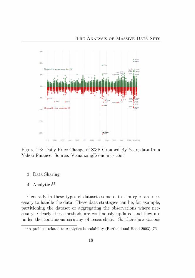
1.3 Daily Price Change of S&P Grouped By Year, datafrom Yahoo Finance. Source: VisualizingEconomics.com 18
1.4 Classical data in a medical data set [82] . . . . . . . . . 23
1.5 Interval data in a mushrooms data set [82] . . . . . . . 24
1.6 Histogram data in a Cholesterol data set Gender × Agecategories: (Billard 2010 [82]) . . . . . . . . . . . . . . 25
1.7 The process of transformation from complex data tablesinto symbolic data or aggregate representation tables [81] 34
1.8 The process of transformation from a relational datatable into a symbolic data table[209] . . . . . . . . . . 37
1.9 Judgement analysis and the interval symbolic data. Mar-chitelli 2009 [486] and Drago et al. 2009 [230] . . . . . 42
1.10 Interval Data Principal Component Analysis and Fi-nancial Data (Drago and Irace in 2004 [231]) . . . . . . 43
1.11 Interval Data Principal Component Analysis and Fi-nancial Data (Drago and Irace in 2004 [231]) . . . . . . 43
XXIII
List of Figures
1.12 Interval Data Principal Component Analysis and Fi-nancial Data (Drago and Irace in 2004 [231]) . . . . . . 44
2.1 High Frequency Data: Trades and quotes dataset (Galli2003 [286]) . . . . . . . . . . . . . . . . . . . . . . . . . 49
2.2 High Frequency Data: Trade durations (Galli 2003 [286]) 55
2.3 High Frequency Data: Quote durations (Galli 2003 [286]) 55
2.4 High Frequency Data: Point Processes (Hautsch 2007)[348]) . . . . . . . . . . . . . . . . . . . . . . . . . . . . 56
2.5 Erroneous observations in High Frequency Data: onespike (Browne 2011 [746]) . . . . . . . . . . . . . . . . 64
2.6 Erroneous observations in High Frequency Data: bidask gapping (Browne 2011 [746]) . . . . . . . . . . . . . 65
3.1 Intervals (Revol 2009 [581]) . . . . . . . . . . . . . . . 83
3.2 A real interval and its parameters lb (lower bound), ub(upper bound), mid (midpoint), rad (radius) and wid(width) Kulpa 2004 [435] . . . . . . . . . . . . . . . . . 84
4.1 Comparing Internal Representations . . . . . . . . . . . 93
4.2 Comparing Complex Internal Representations: Sam-pled data from a N(50,2) summarized by symbolic vari-ables −− Gonzalez-Rivera G. Carlos Mate (2007) [315] 94
4.3 Boxplot time series (BoTS) . . . . . . . . . . . . . . . 97
4.4 Candlestick time series (CTS) . . . . . . . . . . . . . . 98
4.5 Differences between Histogram and Boxplot Data. SourceSAS 9.2 Support Documentation . . . . . . . . . . . . 99
4.6 Histogram Data . . . . . . . . . . . . . . . . . . . . . . 101
4.7 Back to Back Histograms . . . . . . . . . . . . . . . . . 101
4.8 Histogram Time Series (HTS) . . . . . . . . . . . . . . 103
4.9 Clipping Histograms (Risk Visualization) . . . . . . . . 104
XXIV
List of Figures
4.10 Different types of Symbolic Data (Signoriello 2008 [630]). . . . . . . . . . . . . . . . . . . . . . . . . . . . . . . 108
5.1 Kernel density estimation, histogram and rugplot onsimulated data . . . . . . . . . . . . . . . . . . . . . . 112
5.2 Kernel density estimation: illustration of the kernels(Francois 2011 [280]) . . . . . . . . . . . . . . . . . . . 115
5.3 Overlapped Kernel density estimations [793] . . . . . . 117
5.4 Effect of the kernel and the bandwidth choice . . . . . 122
5.5 Effect of the kernel and the bandwidth choice . . . . . 123
5.6 Effect of the kernel and the bandwidth choice (2) . . . 123
5.7 Effect of the kernel and the bandwidth choice (3) . . . 124
5.8 Effect of the kernel and the bandwidth choice (4) . . . 124
5.9 Density Estimation and Profile Risk Indicator computed 127
5.10 Density Estimation and Profile Risk Indicator year: 2007128
5.11 Density Estimation and Profile Risk Indicator computedyear: 2008 . . . . . . . . . . . . . . . . . . . . . . . . . 129
5.12 Density Estimation and Profile Risk Indicator year: 2009130
5.13 Density Estimation and Profile Risk Indicator computedyear: 2010 . . . . . . . . . . . . . . . . . . . . . . . . . 131
5.14 Density Estimation and Profile Risk Indicator computedyear: 2011 . . . . . . . . . . . . . . . . . . . . . . . . . 132
5.15 Radius of the Interval time series (ITS) DJI 1990-2011 132
5.16 Bandwidth for the US Densities computed over the years134
5.17 Implied Volatility for the US Market (VIX Index Indexof volatility expectations (Bloom 2009 [89]) . . . . . . . 137
5.18 Beanplot Time series (BTS) DJI 1990-2001 . . . . . . . 138
6.1 Intra-day price data for Microsoft stock (Zivot 2005 [722])145
6.2 Financial data types with the typical sizes and fre-quency (Dacorogna et al. 2001) [163] . . . . . . . . . . 147
XXV
List of Figures
6.3 Financial data models with the data typical sizes andfrequency (Dacorogna et al. 2001) [163] . . . . . . . . . 149
6.4 The evolution from the boxplot (Harrell et al. 2011 [340])1566.5 Uncertainty in Representations . . . . . . . . . . . . . 1566.6 Simulated beanplot time series (BTS) and turning point
identification . . . . . . . . . . . . . . . . . . . . . . . 1626.7 Dow Jones Index Beanplot Time Series (BTS) consid-
ered for the period 1996-2010 . . . . . . . . . . . . . . 1676.8 Enhanced density data with first and last observation
(in red and blue respectively) . . . . . . . . . . . . . . 1686.9 Enhanced density data with first and last observation:
DJI 1990-2011 (in red and blue respectively) . . . . . . 1696.10 Enhanced density data with first and last observation:
FTSEMIB.MI 2003-2011 (in red and blue respectively) 1706.11 Enhanced Beanplot Trend for the centre: DAX 1990-
2011 (in red and blue, green respectively open, close,centre) . . . . . . . . . . . . . . . . . . . . . . . . . . . 175
6.12 Enhanced Beanplots and Business Cycle Analysis: 3-Year US Unemployment Rates 1948-2011 (in red andblue, first and last observation) . . . . . . . . . . . . . 176
6.13 Enhanced Beanplot and Business Cycle Analysis: 3-Year US Capacity Utilization: Total Industry (TCU)1967-2011 (in red and blue, first and last observation) . 177
6.14 Simulated Beanplot Time Series (BTS) and Kernel Smoothers1806.15 Simulated Beanplot Time Series (BTS) and Smoothing
Splines . . . . . . . . . . . . . . . . . . . . . . . . . . . 1816.16 Comparing different objects: an example on a single
simulated time series: Drago and Scepi 2009 . . . . . . 1876.17 Comparing Boxplot (BoTS) and Beanplot Time Series
(BTS) (Drago Scepi 2009)[237] . . . . . . . . . . . . . . 1886.18 Comparing different interval temporal periods Drago
Scepi 2009 [237] . . . . . . . . . . . . . . . . . . . . . . 189
XXVI
List of Figures
6.19 High Frequency Microsoft Data 1-15 May 2001 (seeDrago and Scepi 2009) . . . . . . . . . . . . . . . . . . 196
6.20 Rolling Beanplots Real Home Price Index 1890-2011using different windows . . . . . . . . . . . . . . . . . . 197
6.21 Rolling Boxplots Real Home Price Index 1890-2011 us-ing different windows . . . . . . . . . . . . . . . . . . . 198
7.1 US Dow Jones differenced time series 1990-2011 . . . . 208
7.2 Beanplot Time Series (BTS) using different TemporalIntervals on an ARIMA(1,1,0) with a structural change 211
7.3 The Data Analysis Cycle . . . . . . . . . . . . . . . . . 214
7.4 Internal and external modelling . . . . . . . . . . . . . 215
7.5 Kernel Density Estimation: computing the area be-tween z1 and z2 . . . . . . . . . . . . . . . . . . . . . . 220
7.6 Highest Density Regions: BVSP Market (differencedseries) year 2010 . . . . . . . . . . . . . . . . . . . . . . 221
7.7 Bovespa Beanplot Time Series -BTS Y C attribute timeseries of the descriptor points 1993-2011 (n = 20) . . . 225
7.8 Bovespa Beanplot Time Series (BTS)XC attribute timeseries of the descriptor points 1993-2011 (n = 20) . . . 226
7.9 Comparing descriptors amongst all the RepresentationTime Series (ITS, BoTS, HTS, BTS and models) . . . 227
7.10 Table of the parameters of the data models (Signoriello2008 [630] . . . . . . . . . . . . . . . . . . . . . . . . . 229
8.1 DJI - Dow Jones Index . . . . . . . . . . . . . . . . . . 242
8.2 DJI - Dow Jones Index . . . . . . . . . . . . . . . . . . 242
8.3 GDAXI - German Dax Index . . . . . . . . . . . . . . 243
8.4 MMX - Major Market Index Mexico . . . . . . . . . . 243
8.5 SSEC - China Stock Market Index . . . . . . . . . . . 244
8.6 N225 - Nikkei Index Japan . . . . . . . . . . . . . . . . 244
XXVII
List of Figures
9.1 Amazon (AMZN) . . . . . . . . . . . . . . . . . . . . . 2719.2 Apple (AAPL) . . . . . . . . . . . . . . . . . . . . . . 2729.3 Goldman Sachs (GS) . . . . . . . . . . . . . . . . . . . 2729.4 Microsoft (MSFT) . . . . . . . . . . . . . . . . . . . . 2739.5 Deutsche Bank (DB) . . . . . . . . . . . . . . . . . . . 2739.6 Morgan Stanley (MS) . . . . . . . . . . . . . . . . . . . 2749.7 Bank of America (BAC) . . . . . . . . . . . . . . . . . 2749.8 Citigroup (C) . . . . . . . . . . . . . . . . . . . . . . . 2759.9 Dow Jones Market . . . . . . . . . . . . . . . . . . . . 2769.10 Dow Jones Market 2007−2008 . . . . . . . . . . . . . . 2779.11 Dow Jones Market 2008−2009 . . . . . . . . . . . . . . 2779.12 Dow Jones Market 2009−2010 . . . . . . . . . . . . . . 2789.13 Dow Jones Market 2010−2011 . . . . . . . . . . . . . . 2789.14 Beanplot Time Series (BTS) Model Based Clustering (1)2949.15 Beanplot Time Series (BTS) Model Based Clustering (2)2959.16 Beanplot Time Series (BTS) Model Based Clustering (3)2969.17 Beanplot Time Series (BTS) Model Based Clustering (4)2979.18 Beanplot Time Series (BTS) Model Based Clustering (5)2989.19 Beanplot Time Series (BTS) Model Based Clustering (6)2999.20 Building Beanplot Prototypes (BPP) from the Beanplot
Time Series (BTS) . . . . . . . . . . . . . . . . . . . . 306
10.1 Beanplot Dow Jones Data 1996-2010 (see Drago andScepi) 2010 . . . . . . . . . . . . . . . . . . . . . . . . 321
10.2 Attribute Time Series . . . . . . . . . . . . . . . . . . . 328
11.1 Scalar dataset . . . . . . . . . . . . . . . . . . . . . . . 33511.2 Visualization of the time series Dow Jones 1990-2011 . 33611.3 Visualization of the time series Bovespa (Brazil) BVSP
1990-2011 . . . . . . . . . . . . . . . . . . . . . . . . . 33611.4 Beanplot time series (BTS) for the Dow Jones DJI 2001-
2011 . . . . . . . . . . . . . . . . . . . . . . . . . . . . 337
XXVIII
List of Figures
11.5 Beanplot Time Series (BTS) Cac 40 (France) FCHI1990-2011 . . . . . . . . . . . . . . . . . . . . . . . . . 338
11.6 Beanplot Time Series (BTS) Bovespa (Brazil) BVSP1990-2011 . . . . . . . . . . . . . . . . . . . . . . . . . 338
11.7 Histogram Time Series (HTS) Dow Jones DJI 1990-2011 33911.8 Histogram Time Series (HTS) Cac 40 FCHI (France)
1990-2011 . . . . . . . . . . . . . . . . . . . . . . . . . 34011.9 Histogram Time Series (HTS) Bovespa (Brazil) BVSP
1990-2011 . . . . . . . . . . . . . . . . . . . . . . . . . 34011.10Interval Time Series (ITS) Dow Jones DJI 1990-2011 . 34111.11Interval Time Series (ITS) Cac 40 (France) FCHI 1990-
2011 . . . . . . . . . . . . . . . . . . . . . . . . . . . . 34111.12Interval Time Series (ITS) Bovespa (Brazil) BVSP 1990-
2011 . . . . . . . . . . . . . . . . . . . . . . . . . . . . 34211.13Boxplot Time Series (BoTS) Dow Jones DJI 2001-2011 34311.14Boxplot Time Series (BoTS) Cac 40 (France) FCHI . . 34311.15Boxplot Time Series (BoTS) Bovespa (Brazil) BVSP
2001-2011 . . . . . . . . . . . . . . . . . . . . . . . . . 34411.16Clustering original time series (2000-2011) . . . . . . . 34811.17Clustering using coordinates correlation distance dis-
similarity matrix . . . . . . . . . . . . . . . . . . . . . 34911.18Clustering using coordinates correlation distance aver-
age method . . . . . . . . . . . . . . . . . . . . . . . . 34911.19Clustering using coordinates correlation distance single
method . . . . . . . . . . . . . . . . . . . . . . . . . . 35011.20Clustering using coordinates correlation distance Mc-
Quitty method . . . . . . . . . . . . . . . . . . . . . . 35011.21Clustering using coordinates correlation distance Com-
plete method . . . . . . . . . . . . . . . . . . . . . . . 35111.22Clustering using correlation distance - Centroid method 35111.23Factor 2: correlation distance: (average) . . . . . . . . 35211.24Factor 2: correlation distance: (single) . . . . . . . . . 352
XXIX
List of Figures
11.25Clustering Interval Time Series (ITS) on centers: longperiod of interval . . . . . . . . . . . . . . . . . . . . . 353
11.26Clustering Interval Time Series (ITS) on centers: shortperiod of interval . . . . . . . . . . . . . . . . . . . . . 353
11.27Clustering Beanplot time series (BTS) using the modeldistance (method average) . . . . . . . . . . . . . . . . 354
11.28Differenced time series from the Beanplot Clusteringprocess . . . . . . . . . . . . . . . . . . . . . . . . . . . 355
11.29Interval attribute time series DJI (first 100 observations)35811.30Boxplot attribute time series DJI 1900-2011 . . . . . . 35811.31Forecasting Beanplot time series (BTS) using the mix-
ture: coefficients estimation . . . . . . . . . . . . . . . 36111.32Forecasting beanplot time series (BTS) using the mix-
tures: factor time series . . . . . . . . . . . . . . . . . . 362
XXX
Introduction
Big data and huge or massive datasets are becoming ubiquitous. Atthe same time there is a growth of applications that collect data in realtime, for example internet databases or financial data. So the generalproblem nowadays is the need to work extensively with huge data. Inthese cases, it is not always possible to store the data in such kinds ofdatabases.
In all cases, data represents value that can be exploited through theextraction of the information contained within it for business aims. Sothe challenge for Data Science is to consider new methods to extractthe information on huge datasets and to use it for the creation of value.
In this work the main focus is on high frequency data. These datarely on phenomena that generate unequally spaced observations, withthe particular characteristics of an overwhelming number of observa-tions over time, erroneous data, price discreteness, volatility, etc.
Recently, in literature new types of structured data have been pro-posed, which have an internal variability: intervals, boxplots and his-tograms. We introduce this structured data as representation in con-crete problems and applications related to such kind of data.
In particular, the applicability of these representations to time se-ries analysis of very long time series has been studied. In the mostrecent literature there has been the application of time series repre-sentations using the Histogram and Interval Data, these have been
Introduction
applied to real problems like the analysis of financial time series, andthere has been the analysis of time series related to other sectors likeenergy, etc.
A relevant problem is the temporal interval to choose in order tooptimally define structured data. Various options are possible: hour,day, week, month, and year. A clear answer depends on the specificapplication we are interested in. So, sometimes, it may be useful toconsider structured data, by considering the hour for trading applica-tions, and sometimes it could be useful to consider a bigger temporalinterval: for example in analyses useful for risk management. There-fore, a specific best temporal interval does not exist. The choice canalso influence the methods used in the analysis, as we will see duringthe thesis. In the thesis we propose a new structured representation,based on special data as densities or beanplots: the density (or thebeanplot) time series. The density time series (or the beanplot timeseries BTS) is particularly useful for exploratory data analysis of highfrequency data in which we can discover important information thatcould otherwise be lost. This type of representation could be par-ticularly fruitful when we have a higher number of high frequencyobservations for each structured data.
In the thesis, starting from this type of visualization we consider theneed to model the data. The aim of the modelling is for both cluster-ing and forecasting. In particular, we propose two types of approachesand we show the advantages and disadvantages. The proposed coef-ficients estimation and representation by descriptor points allow usto use some specific forecasting models and to analyze in depth thestructural changes and the existence of groups of beanplots time serieswith similar characteristics over time.
In forecasting, the selection of the best information set availablein the models is crucial. With regard to this there is the use of analgorithm to select the best information available in the past, whichwe use, and which can be applied to update the predictions. The the-
2
Introduction
sis is accompanied by simulation exercises as well as by applicationsand examples based on real data. All methods proposed have beenimplemented using algorithms written in R code (shown in the Ap-pendices).
The thesis is organized as follows:Part I: The State of the ArtChapter 1. We consider the basic problems with huge data and the
evolution that they have undergone in recent years. We analyze theresponses of methods for the analysis of this database. In particular,the analysis of data such as interval data to boxplots or histogramis considered as a possibility to account for large databases withoutthe information loss due to the aggregation of the data. This chapterreviews various methods and techniques related to the internal rep-resentations and the symbolic data. Then, the methods for startingfrom a relatively huge data base leading to operational data bases withdata that serve as internal representations are described. The final in-ternal representation data can be modelled internally to obtain thedata models. In any case these data are characterized by the intra-period variation.
Chapter 2. The database of the new type (as seen in Chapter 1),with specific reference to the financial sector, is analyzed. In par-ticular, an innovation of recent years has been that of making useof high frequency data (High Frequency Data) that calls for specifictechniques in their econometric and statistical treatment. In the sameway, the characteristics of financial time series which require the sameuse of specific techniques for data analysis are analyzed.
Chapter 3. An interval is given as the first type of internal repre-sentation that can be considered and analyzed. In particular, thesetypes of representations have an algebra that is reviewed as the basisof the techniques considered later in the thesis. The evolution of thetechniques of interval data (which are compared with the techniquesproposed later in the thesis) is then discussed. In this sense, the tech-
3
Introduction
niques for analyzing time series data interval are considered.In Chapter 4, representations based on different data types other
than Intervals, for example boxplots, histograms and more recentlycandlestick charts, are considered. Here we consider the histogramalgebra as an extension of the interval algebra. At the same time, inthe chapter the developments in time series analysis of boxplots orhistograms are considered. The final problem is the internal represen-tation that could be used: in particular the choice of the representa-tions in concrete problems. We propose some considerations on thechoice of the statistical data, which are extensively considered duringthe second part of the work.
Chapter 5. A clear alternative to the use of data histogram arenew types of data defined as data density that produce data using themethods of Kernel Density Estimation. In particular, such a method-ology allows us to obtain a smoother image of the underlying datastructure, by choosing appropriate bandwidth and kernel. Using den-sity data offer some advantages with respect to intervals or histogramdata in main precise applications: In particular, for large databasethis type of data can approximate in a better way histogram represen-tation. The Kernel Density Estimation is analysed and its character-istics and properties evaluated. In particular, we focus on the choiceof bandwidth and kernel.
Part II: New Developments and New MethodsChapter 6. From the Kernel Density Estimation of Chapter 5 the
data given in Beanplot density used in the thesis is introduced anddefined. In particular, we introduce the time-series data density (orBeanplot). Then we analyze the ability to display and explore thisdata in comparison with objects of different types, in particular indifferent data structures. The chapter is accompanied by simulationexercises that consider simulated high frequency data comparing dif-ferent types of time series of complex objects.
Chapter 7. In this chapter methods for analyzing time series of
4
Introduction
Beanplot Data Models are considered. In particular, we describe twotypes of approaches: the first leading to a fundamental description ofthe dynamics of Beanplots over time, and the second, which separatesthe structural aspect of Beanplots compared to the ”noise” (or theerror). It is assumed that the data are characterized by patterns ofMixture Models. In this sense, the coefficients are used to capture theevolution of these models over time. The models, therefore, can high-light the change in inter -or intra-temporal of huge data and replacethe series of Beanplots with coefficients (which are considered in theirtemporal evolution).
Chapter 8. At this point, there is the need to take into account thetime series of attributes and trajectories obtained to build appropriatepredictive models. In particular, the identification of the forecastingmodel to estimate each point of the series. In this case there can bethe need to use different approaches in forecasting and combine theforecasts obtained in the procedure. The goal is to minimize the riskand uncertainty in the choice of a unique forecasting model in thepresence of very volatile data, structural changes or model parameterchanges (Parameter Drift). Finally, a search algorithm is applied toidentify the range of observations to be used in the optimal forecastingmodel.
Chapter 9. We analyze the problems of Beanplot Clustering fortime series. In particular, starting from the time series of attributesobtained we synthesize the beanplot time series (BTS) by using theTime Series Factor Analysis-TSFA, which synthesize the Beanplot dy-namics over time.
For the Cluster Analysis, various types of Correlational Distancesfor Beanplot time series (BTS) have been considered, whereas suitabledistance model (as proposed by Romano, Giordano and Lauro) havebeen used when the Beanplot are represented.
Chapter 10. In this chapter the performance of both internal andexternal models are analysed on the basis of indices of the adequacy of
5

Introduction
the models. In particular, the evaluation and validation of models canlead to the respecification of both the internal models and the externalmodels referred to in Chapters 7 (visualization and data exploration)8 and 9 (regarding the identification and construction of the externalmodels).In Chapter 10 we consider real case studies in the field of FinancialMarket Monitoring, Asset Allocation, Statistical Arbitrage and RiskManagement using the methods seen in the thesis.
In the final Chapter there are conclusions and future developments.In the Appendices there are the R codes which replicate the proce-
dures proposed and analyzed during the PhD thesis.
6

Part I
Data: The State of The Art
7

Chapter 1
The Analysis of MassiveData Sets
”From now on, the key is knowledge. The world is not becoming laborintensive, not material intensive, not energy intensive, but knowledgeintensive” says Peter Drucker, the authoritative manager and consul-tant in 1992 [238]1.
At the same time it was recently stated that ”The statistics profes-sion has reached a tipping point. The need for valid statistical toolsis greater than ever; data sets are massive, often measuring hundredsof thousands of measurements for a single subject. The field is readyfor a revolution, one driven by clear, objective benchmarks by whichtools can be evaluated2..” (Der Laan, Hsu and Peace 2010 [672]).
In this sense, the big data are becoming a growing flow in everyarea of the economy (McKinsey 2011 [499] and the Economist [655]
1Bifet Kirby 2009 [80]2In this sense there is the birth of ”Data Science”. See Loukides (2010) [468]
for a detailed analysis about the reasons and the prospectives of the discipline.The author explains in the Report that ”the future belongs to the companies andpeople that turn data into products”
The Analysis of Massive Data Sets
and Science 2011 [616]3. These data are typically timeliness, and inreal time (Mason 2011 [490]) intrinsically a value4
In particular big data are datasets which grow in a way that aredifficult to be managed using on-hand database management. Diffi-culties can be considered in a wide sense, for example in informationcapture, in data storage as in Kusnetzky 2010 [438], in the informationextraction and search using adequate tools, in sharing information andreporting, in analytical methods (Vance 2010 [674]) and in the visual-ization of these data5 (Boyd and Crawford 2011 [107])
McKinsey 2011 [499] gives a definition of the relevance of the BigData concept: ”Big data refers to datasets whose size is beyond theability of typical database software to capture, store, manage, andanalyze”6. The definition is intentionally subjective and incorporatesa moving definition of how big a dataset needs to be in order to beconsidered big data i.e. we do not define big data in terms of beinglarger than a certain number of terabytes (thousands of gigabytes).
It is probable to assume that as technology advances7 over time then
3In particular the big datasets are interesting for the problems which they cansolve in business and for the capability to create value, the concept is clear in LevRam (2011) [454] in which the author interviews Jim Goodnight, CEO of softwaremaker SAS
4Madsen 2011 [474] ”...In their data there is a competitive advantage”5The evaluations on the problems of Big Data given, its enormous advantages
are growing; see for example: The Economist 2010 [655], [2] and [730]6Manovich 2011 observes: ”There is little doubt that the quantities of data
now available are indeed large, but thats not the most relevant characteristic ofthis new data ecosystem. Big Data is notable not because of its size, but becauseof its relationality to other data. Due to efforts to mine and aggregate data, BigData is fundamentally networked. Its value comes from the patterns that canbe derived by making connections between pieces of data, about an individual,about individuals in relation to others, about groups of people, or simply aboutthe structure of information itself..”
7See for example Miller 2010 [506]: ”Cloud computing and open source soft-ware are fueling the data and analytics binge. The cloud allows businesses to lease
10
the size of datasets that qualify as big data will also increase8 Alsonote that the definition can vary by sector, depending on what kindsof software tools are commonly available and what sizes of datasetsare common in a particular industry. With those caveats, big datain many sectors today will range from a dozen terabytes to multiplepetabythes (thousands of terabytes).
By considering this point it is necessary to stress the fact that thevolume of data is growing at an exponential rate (see Mckinsey 2011[499]). There are in that sense various research works investigatingthis growth over time. Lyman and Varian, as reported by the McKin-sey Report in 2011 [499],”estimated that the size of new data stored,doubled from 1999 to 2002 at a compound annual growth rate of 25percent”.
In that way, in recent years huge datasets have become ubiqui-tous because of the number of systems or applications which producelarge volumes of data (see Aggarwal 2007 [7]). In particular duringthe past few years it has been very easy to collect huge amounts ofdata, also defined as ”massive data-sets”. Examples [576] (see Raykar
computing power when and as they need it, rather than purchase expensive infras-tructure. And the combination of the R Project for Statistical Computing and theApache Hadoop project that provides for reliable, scalable, distributed comput-ing, enables networks of PCS to analyze volumes of data that in the past requiredsupercomputers. With the Hadoop platform, Visa recently mined two years ofdata, over 73 billion transactions amounting to 36 terabytes. The processing timedropped from one month to 13 minutes”
8Where the size of data sets increase they become more and more real time,see Babcock [52] 2006: ”But databases aren’t just getting bigger. They’re alsobecoming more real time. Wal-Mart Stores Inc. refreshes sales data hourly, addinga billion rows of data a day, allowing more complex searches. EBay Inc. letsinsiders search auction data over short time periods to get deeper insight intowhat affects customer behavior”. The problem is well known also for financialdata in which econometric techniques to face high frequency data use some specialtechniques in real time, see: Pesaran and Timmermann 2004 [558]
11
The Analysis of Massive Data Sets
2007) can include as the author did, genome sequencing, astronomicaldatabases, internet databases, medical databases, financial records,weather reports, audio and video data. At the same time, it is possi-ble to consider in practice other data typologies (see Huang KecmanKopriva 2006 [372]).
So where modern database are diffused everywhere in industrialcompanies and public administration (Diday 2008 [209]) they tend toincrease dramatically their size and the technical advances in databasesand information systems are continuous (see for example the annualconferences organized in very large databases (Very Large Data BaseEndowment Inc (2010) [683]) and the O’Reilly Strata Conference (2011)[541]).
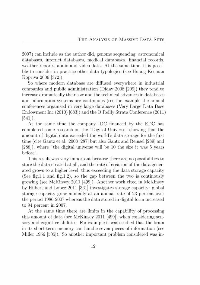
At the same time the company IDC financed by the EDC hascompleted some research on the ”Digital Universe” showing that theamount of digital data exceeded the world’s data storage for the firsttime (cite Gantz et al. 2008 [287] but also Gantz and Reinsel [289] and[288]), where ”the digital universe will be 10 the size it was 5 yearsbefore”.
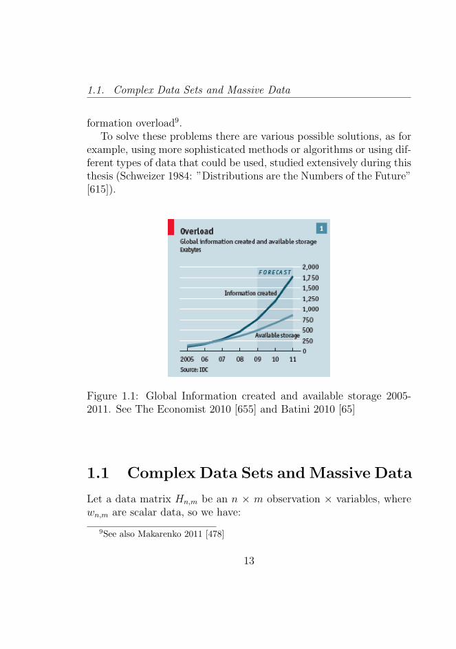
This result was very important because there are no possibilities tostore the data created at all, and the rate of creation of the data gener-ated grows to a higher level, thus exceeding the data storage capacity(See fig.1.1 and fig.1.2), so the gap between the two is continouslygrowing (see McKinsey 2011 [499]). Another work cited in McKinseyby Hilbert and Lopez 2011 [361] investigates storage capacity: globalstorage capacity grew annually at an annual rate of 23 percent overthe period 1986-2007 whereas the data stored in digital form increasedto 94 percent in 2007.
At the same time there are limits in the capability of processingthis amount of data (see McKinsey 2011 [499]) when considering sen-sory and cognitive abilities. For example it was studied that the brainin its short-term memory can handle seven pieces of information (seeMiller 1956 [505]). So another important problem considered was in-
12
1.1. Complex Data Sets and Massive Data
formation overload9.To solve these problems there are various possible solutions, as for
example, using more sophisticated methods or algorithms or using dif-ferent types of data that could be used, studied extensively during thisthesis (Schweizer 1984: ”Distributions are the Numbers of the Future”[615]).
Figure 1.1: Global Information created and available storage 2005-2011. See The Economist 2010 [655] and Batini 2010 [65]
1.1 Complex Data Sets and Massive Data
Let a data matrix Hn,m be an n × m observation × variables, wherewn,m are scalar data, so we have:
9See also Makarenko 2011 [478]
13
The Analysis of Massive Data Sets
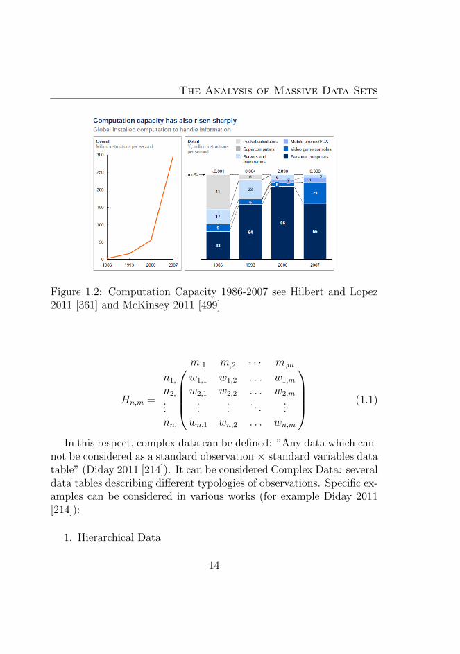
Figure 1.2: Computation Capacity 1986-2007 see Hilbert and Lopez2011 [361] and McKinsey 2011 [499]
Hn,m =
m,1 m,2 · · · m,m
n1, w1,1 w1,2 . . . w1,m
n2, w2,1 w2,2 . . . w2,m...
......
. . ....
nn, wn,1 wn,2 . . . wn,m
(1.1)
In this respect, complex data can be defined: ”Any data which can-not be considered as a standard observation × standard variables datatable” (Diday 2011 [214]). It can be considered Complex Data: severaldata tables describing different typologies of observations. Specific ex-amples can be considered in various works (for example Diday 2011[214]):
1. Hierarchical Data
14
1.1. Complex Data Sets and Massive Data
2. Textual Data
3. Time Series Data in each cell
4. Multisource Data Tables (Data Fusion)
Massive Data, are datasets of huge dimensions, and they come frommany sources10, and they can be generated by various devices likesensors, cameras, microphones, pieces of software (see Huang KecmanKopriva 2006 [372] and Diday 2008 [209]). Another important domain,in the enormous increase of the data, can be considered due to DataStreams Applications (Aggarwal 2007 [7] and Balzanella Irpino Verde2010 [56]).
A typical example of the differences of the data stream applicationswith respect to the data mining procedures is given by Domingos Hul-ten 2010 [224], data, in particular are collected, in various applicationsfaster than it is possible to mine (Balzanella Irpino Verde 2010 [56]).In this respect, to avoid data losses it is necessary to pass to systemsthat are able to mine continuously the high-volume, open-ended datastreams at the time they are available.
Clearly in other situations, also with huge data sets it is possibleto use the classical data mining approach. Data are everywhere so theapproach can be generalized to different fields.
A typical example of complex data are also High Frequency finan-cial data (See Dacorogna et al. 2001) [163]. In finance the innovationwas typically due to the introduction of Tick Data (also defined HighFrequency Data) that made it possible to develop trading strategiestaking into account Intraday market movements. The empirical studyof these dynamics would be very beneficial for an understanding of the
10In particular the relevant information comes from many data sources where theproblem, today, becomes how to combine this information (Ras Tsumoto Zighed2005 [577]
15
The Analysis of Massive Data Sets
markets and the reduction of the associated risk of the price fluctua-tions (see Engle Russell 2009 [254]). High Frequency Data in particularcan help to forecast risk (see for example Kaminska 2008 [415]).
At the same time complex time series can be also obtained by con-sidering some time series in large data sets (for example in Financeor in Energy applications like Load Forecasting) where the series arespecifically characterized by lower frequency but at the same time by”complex” characteristics (spikes, nonlinearities, high volatility etc.).In this sense it possible to consider the approach of the time series ascomplex data (Diday 2008 [209]).
It is important to stress the fact that using large datasets is a spe-cific need (and sampling in that case does not help), because the realdata are huge and continually flowing, but at the same time it is aspecific advantage (the creation of the value).
There are cases in which using big datasets can be very useful andthis is typical for exploratory studies where in that case it is not suffi-cient to define some statistical relationships that could be adequatelyestimated or tested (see Benzecrı 1973 [74] Lebart Morineau Piron1995 [452] Saporta 1990 [607] Gherghi Lauro 2002 [300] and Bolasco1999 [100]).
At the same time it is possible to consider some other cases in whichdata are overwhelming and theoretical models need to adequately faceup to the existing data (see Sanchez Ubeda 1999 [606]). In thesecases big datasets can be useful to generate some hypothesis withdata (Tukey 1977 [670]).
The general case and the most classical case in using big databasesis Data Mining or Business Intelligence (Giudici 2006 [312]). In thiscase large datasets can be used to extract information and to extractthe knowledge present in data. Here, the idea is that of using thisspecific knowledge to obtain some relevant business indications. In
16
1.1. Complex Data Sets and Massive Data
this case the data are considered a specific richness to use11 .The first and direct consequence of the data, in this sense is that
humans cannot handle and manage such a massive quantity of data,which are usually collected in the numeric shape as the huge rectangu-lar or squared data matrices (see Huan Kecman Kopriva 2006) [372].The challenge in this sense is using specific systems that automaticallyextract the information from the raw data to permit better decisions(see Raykar 2007 [576]).
In this case it is necessary to apply some specific statistical tech-niques in order to achieve the data management and the knowledgeextraction, that is, therefore we need to to use specific statistical tech-niques to handle these data sets.
On the contrary, using the single valued variables (using for exam-ple some form of data aggregation) brings information loss. In thegraph there is an example in which a large data set does not allow theobservation of the data structure of the underlying financial data (Seefig.1.3).
1.1.1 Characteristics of Complex Data Sets andMassive Data
Massive data are characterized by an overwhelming number of obser-vations and\or variables. Problems in these datasets are related to(see McKinsey 2011 [499]):
1. Data Storage
2. Data Search and Extraction
11Data richness allows the improvement of data analysis to a certain extent inorder to improve the data analysis, see for example: Linoff Berry 2011 [461] andWeiss Indurkhya 1996 [696]
17
The Analysis of Massive Data Sets
Figure 1.3: Daily Price Change of S&P Grouped By Year, data fromYahoo Finance. Source: VisualizingEconomics.com
3. Data Sharing
4. Analytics12
Generally in these types of datasets some data strategies are nec-essary to handle the data. These data strategies can be, for example,partitioning the dataset or aggregating the observations where nec-essary. Clearly these methods are continously updated and they areunder the continuous scrutiny of researchers. So there are various
12A problem related to Analytics is scalability (Berthold and Hand 2003) [76]
18
1.1. Complex Data Sets and Massive Data
techniques and algorithms that could be used in these cases13.Diday 2011 [214] states that a solution could be possible in differen-
tiating standard scalar observations (classical data) from the symbolicobservations (data that represents an internal structured variation andwhich are structured). In that sense we can have: ”Standard observa-tions like a player, a fund, a stock... Symbolic observations: Classes: aplayer subset, a subset of funds, stocks... Categories: American funds,European funds, ... Concepts: an intent: volatile American funds, anextent: the volatile American funds of a given data base.”
There are important cases in which it is particularly useful to usethe concepts instead of classical data, cases for example in which weare considering data where in itself the concept could be important,and cases in which we need to manage a data fusion of different datatables or datasets.
In particular what are the advantages of using Internal Represen-tations or Symbolic Data? Diday 2011 [214] states them to be these:
1. Considering the right generality level of a collective data withoutinformation loss.
2. Reducing the data set size and so reducing the number of vari-ables and observations (reducing computational costs of the anal-yses).
3. Mitigating the problem of missing data.
4. Ability to ”extract simplified knowledge and decision from com-plex data”.
5. Solving the problems related to confidentiality.
6. ”Facilitate interpretation of results”: decision trees, factorialanalysis, new graphic kinds.
13McKinsey 2001 [499]
19
The Analysis of Massive Data Sets
7. ”Extent Data Mining and Statistics to new kinds of data withmany industrial applications”.
There are some cases in which data sets are characterized by manyoutliers or missing data. So it could be important to provide a dataimputation (in the case of missing data) to allow a safe use of theaggregate representations. In fact, sometimes missing values are notdistributed at random during the dataset and they are missing follow-ing a pattern.
In the case of missing data (that could be considered not a ran-dom), they need to be substituted using some statistical methods14.Various strategies could be considered for the original missing data:see Little and Rubin 1987 [464], Allison 2001 [15] and Howell 2007[367].
In any case, a preliminary analysis on the data to detect the outliersand an imputation strategy (if there are missing data) is necessary. Infact both outliers and missing data can affect the statistical analysis.
1.1.2 Statistical Methods, Strategies and Algo-rithms for Massive Data Sets
Later we will analyse in depth statistical methods that consider data asrepresentations (interval, histograms etc.). Many different approachesare considered in literature that could be used considering scalar datain massive data sets15. It is important to note that we can aggregateor not the entire dataset. In particular one possibility is to work onthe entire dataset without any type of aggregation.
Various strategies and methods can be considered (see Giudici 2006
14Zuccolotto 2011 [725] for an approach on symbolic data15A review and a presentation of some approaches is in Rajaraman, A. and
Ullman D.J. (2010) [572] Gaber, Zaslavsky and Krishnaswamy (2005) [285]
20
1.2. Analysing data using Aggregate Representations
[312]), alternatively we can consider many methods together (strate-gies) as for example in Gherghi Lauro 2002 [300] and Bolasco 1999[100] in which we use more methods sequentially. So in these cases wecan define different strategies for the analysis in which, for example,we reduce a dataset using a factorial method and after classify thestatistical units16.
Relevant methods used to analyze Big Data in Businesses todayare enumerated in the McKinsey 2011 [499] Report. This point needsto remain open because the approaches and advances in literature andin business evolve very quickly.
1.2 Analysing data using Aggregate Rep-
resentations
A different approach is related to that considering Aggregate Rep-resentations (the entire representation expressing variation for thedata disaggregated) and working with methods like those in SymbolicData Analysis (see for example Diday 2008 [209] where Valova andNoirhomme Fraiture consider explicitly the case of massive data andSymbolic Data Analysis [673]).
In these cases we directly consider some types of new data, as forexample intervals, histograms etc. These new data are structured andexpress internal variation on the single data. In particular the datacan be defined symbolic data if they contain more complex informa-tion than scalar data (they can characterized by internal variation andcould be structured Diday 2002 [207]).
In that sense the symbolic data can summarize massive data bases
16It is possible to consider the approach of data analysis in SPAD softwarefor example in which we perform the statistical and data mining analysis using”chains” or sequences of different methodologies see: Coheris 2011 [737]
21
The Analysis of Massive Data Sets
by considering their Concepts. They can be defined as first units andbe characterized by a specific set of properties defined as ”intent” and”extent” that could be seen by the set of the units which suits theseproperties. The Concept could be described by symbolic data whichcan be intervals, histograms, etc.
The characteristics of the data allow us to bear in mind the internalvariation of the ”extent” by considering the different Concepts (Diday2002 [207] and also 2008 [210]).
There are important cases in which Concepts are relevant and theywere described by Diday in 2011 [214]. Symbolic Objects can be rel-evant in modelling the Concept as shown in Lauro and Verde 2009[449]:
1. When there is a specific interest on the Concepts (for examplewhen the data analyis is based on the respect to the single units)
2. ”When the categories of the class variable to explain are consid-ered as new units and described by explanatory symbolic vari-ables”
3. In the case of data funsion of multisource tables
Another important preliminary analysis is the optimality of theConcept chosen17
1.2.1 Scalar Data and their Aggregate Represen-tation
So we can specifically define the complex data as, for example, theInterval and the Histogram Value Data: complex data are data thatcannot be considered standard observation × variables or n×m data
17Diday 2011 [214]
22
1.2. Analysing data using Aggregate Representations
tables, interval and histogram data are typically data in which thereexists a variation inside the classes of standard observation (see alsoDiday 2010 [211] ). In that case, by starting from the initial massivedata sets, each cell of the data table can contain an interval, a boxplot,an histogram, a bar chart, a distribution etc.
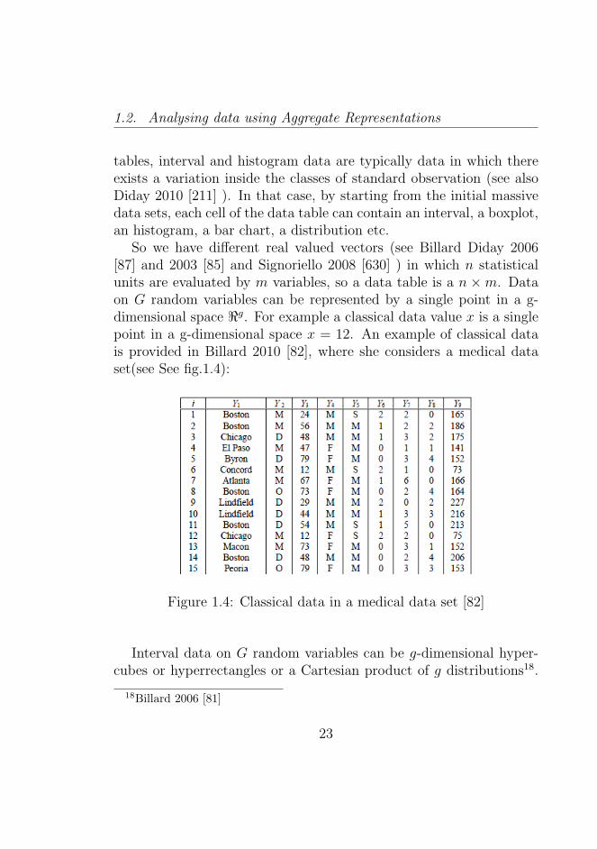
So we have different real valued vectors (see Billard Diday 2006[87] and 2003 [85] and Signoriello 2008 [630] ) in which n statisticalunits are evaluated by m variables, so a data table is a n ×m. Dataon G random variables can be represented by a single point in a g-dimensional space <g. For example a classical data value x is a singlepoint in a g-dimensional space x = 12. An example of classical datais provided in Billard 2010 [82], where she considers a medical dataset(see See fig.1.4):
Figure 1.4: Classical data in a medical data set [82]
Interval data on G random variables can be g-dimensional hyper-cubes or hyperrectangles or a Cartesian product of g distributions18.
18Billard 2006 [81]
23
The Analysis of Massive Data Sets
That is, by considering the case of the intervals [x1, x1] and also [x2, x2]where x is the interval lower bound and x the interval upper bound,with g = 2 where the random variables take values over the intervals.The data value in this case is the rectangle R = [x1, x1]× [x2, x2] andvertices of R are: (x1, x1), (x1, x2), (x2, x1) and (x2, x2).
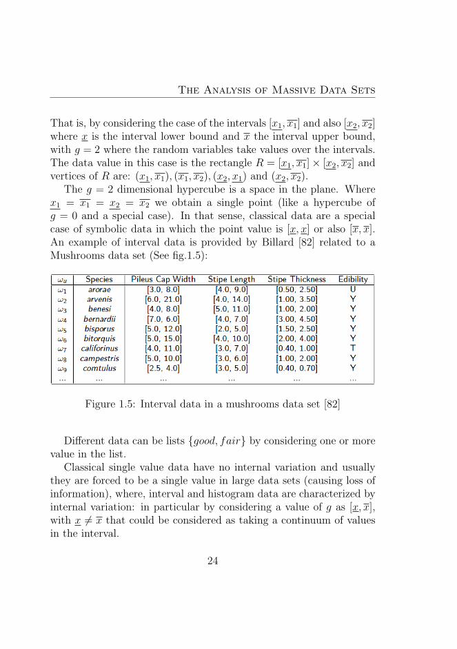
The g = 2 dimensional hypercube is a space in the plane. Wherex1 = x1 = x2 = x2 we obtain a single point (like a hypercube ofg = 0 and a special case). In that sense, classical data are a specialcase of symbolic data in which the point value is [x, x] or also [x, x].An example of interval data is provided by Billard [82] related to aMushrooms data set (See fig.1.5):
Figure 1.5: Interval data in a mushrooms data set [82]
Different data can be lists good, fair by considering one or morevalue in the list.
Classical single value data have no internal variation and usuallythey are forced to be a single value in large data sets (causing loss ofinformation), where, interval and histogram data are characterized byinternal variation: in particular by considering a value of g as [x, x],with x 6= x that could be considered as taking a continuum of valuesin the interval.
24
1.2. Analysing data using Aggregate Representations
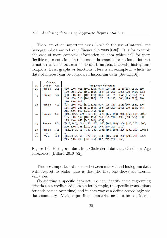
There are other important cases in which the use of interval andhistogram data are relevant (Signoriello 2008 [630]). It is for examplethe case of more complex information in data which call for moreflexible representation. In this sense, the exact information of interestis not a real value but can be chosen from sets, intervals, histograms,boxplots, trees, graphs or functions. Here is an example in which thedata of interest can be considered histogram data (See fig.1.6):
Figure 1.6: Histogram data in a Cholesterol data set Gender × Agecategories: (Billard 2010 [82])
The most important difference between interval and histogram datawith respect to scalar data is that the first one shows an internalvariation.
Considering a specific data set, we can identify some regroupingcriteria (in a credit card data set for example, the specific transactionsfor each person over time) and in that way can define accordingly thedata summary. Various possible summaries need to be considered.
25
The Analysis of Massive Data Sets
In each of these examples the data can be transformed into singlevalued data but interval data shows a higher complexity. Billard andDiday 2010 [88] in this sense make various examples: transactionsby dollars spent [5, 1200] or a different summary by type of purchase(gas, clothes, food, ...) or, by type and expenditure ( gas [30, 60]),food, [25, 105] ...). In all these examples it is necessary to consider aswell a temporal component as the summarized values over the time t,for example transaction by dollar in various periods.
Interval and Histogram data can capture specific variation overtime t, important in their own right on any data set. Variables g canbe collected as an interval over time t (for example [88]: pulse rateat time t ( [60, 72] ), at time t + 1 ( [62, 74] ) systolic blood pressureat t ( [120, 130]), at t + 1 became ( [122, 132]) and diastolic bloodpressure ([85, 90]) at t and ([87, 93]) for each of n = 100 patients (or, forn = 12 million patients). Alternatively, we can consider the evolutionover the time t of different classes of n = 31 students that could becharacterized by boxplots, histograms or distributions of their marksfor each of several variables g at time t (for example mathematics,statistics and biology).The information loss in aggregate data is shown by Billard 2006 in[81]. In fact it is possible to show that, considering three realizationsof a random variable G = weight (accordingly with the considereddataset), we have G1 = 135, G2 = [132, 138], G3 = [129, 141]. It ispossible to consider these three samples each of size n = 1. Bertrandand Goupil 2000 [77] show that S2 is specifically the sample variance ofeach variable G under the assumption of uniformly distributed valuesin each interval, where: Pu = [xu, xu], u = 1...n. We have:
S2 =1
3n
n∑u=1
(x2u + xu · xu + x2
u)−1
4n2
n∑u=1
[xu + xu]2 (1.2)
So we obtain that the sample mean is P 1 = P 2 = P 3 where
26
1.2. Analysing data using Aggregate Representations
S21 = 0, S2
2 = 3, S23 = 12. For the basic statistics procedure in
Interval Data Analysis see also Gioia Lauro 2005 [310] and Billard[82]. The internal variation of the interval and histogram observationdetermines the difference between the three results. In this case wecan show that it is necessary to take into account the internal varia-tion considering interval and histogram data.
It is important to note that in all these cases these types of data areinherently rich in nature, infact in these cases data are characterizedand can be compared by not only a single value, but at the same timeby a location (say, the central value), a size (the internal variation)and a shape (the exact form of the distribution).
It is possible to find a specific link between data collection and itsrepresentation (for example, after a query in a database) it is possibleto find the same link between the interval data and its interpretation.Data that show relevant internal variation (due to the data internalheterogeneity) need to be analysed using specific statistical techniques(interval and histogram valued data analysis techniques in particular).
Interval and Histogram value data arise in different ways. In factthe data we have considered are natively interval and histogram (theyshow an internal variation that could not be represented as a scalardata). So the single values do not represent faithfully the data wewant to consider. If a data is natively an interval and we force thedata to be a single-valued data we are forcing the data to be scalarand we are not considering its real nature of interval. In this sensethe use of the interval data is determined by the nature of the originaldata
In other cases we can be specifically interested not in the singlevalue but in the specific variation, because the single value might notbe so relevant (due for example to fluctuations of the measurements).In that sense there are real cases in which it is very difficult to mea-sure a specific phenomenon as a single scalar or value (due to a specificreason) and in that case single observations would not be relevant. In
27
The Analysis of Massive Data Sets
this case an interval or a symbolic data can capture in a better mannera real phenomenon by considering the intervals of the measurements.
Fluctuations can be related specifically to errors both in the dataand in the solutions. Gioia and Lauro 2005 [310] provide some exam-ples of these errors:
1. Measurement errors: where the measured value of a physicalquantity x may be different from the exact value of the quantity
2. Computation errors: when round errors make a distortion fromthe true results due to the finite precision of the computers
3. Errors due to uncertainty in the data: the value of a specificdata cannot be measured precisely in a physical way
Billard and Diday 2010 [88] show other cases in which there areno relevant errors in data, but actual technologies do not allow theperformance of the requested computations.
So we can have a fourth case in which the use of symbolic data isimportant. By considering n observations (when n is very large withhundred of thousands or more) with m variables (at the same timewith m hundred or more), so by taking into account a n ×m matrixH in an inversion computation H−1 the computational burden can berelevant.
It is important to note that also where computer capabilities ex-pand at the same time (larger computation of H−1 at a time, theburden assuming a growth either of n and m will be relevant) it isimportant to consider the growth of the dataset size and so the sizeof the n×m matrix H (Gantz et al. 2008 [287]).
The last reason for the use of symbolic data is when there areproblems with results, where there is aggregated data that does notfaithfully confirm the results obtained by disaggregated data. The re-sult is well known for example in High Frequency Data in which there
28
1.2. Analysing data using Aggregate Representations
can be explicit differences in analyses considering different types of ag-gregations, for example, frequencies (see Dacorogna et al. 2001 [163]).Differences between results using aggregated and disaggregated dataare well known as well in Econometric literature (aggregation bias).For example in the presence of outliers it can be very dangerous touse data aggregations because the methods used may not be robust(in a statistical sense) and results used may not faithfully representthe ”real” data.
At the same time, aggregating data presenting outliers can lead tothe loss of the information related to the original problem. In thissense outliers cannot be detected in the aggregated data, or they canbe masked by the data structure.
Infact, it is important to note that aggregation cannot capture thereal structure of the data but tends to force data to have a single value.Also by considering more complex aggregation methods, for examplerobust methods, we lose information. For this reason, Schweizer 1984[615] says that ” the distributions are the number of the future!”, thuswe need to consider statistical approaches that directly use distribu-tion data. In these cases we need to consider these data as internalrepresentations or symbolic data.
1.2.2 Sources for Aggregate Representations andSymbolic Data
Symbolic data can be obtained in the process of data reduction froma huge dataset. Any query in a database can produce descriptivevariables and categories. Diday [207] shows, for example, categories(SPC) crossed with categories of age (Age) and regions (Reg). So itis possible to obtain a new categorical variable of cardinality |SPC|×|Age| × |Reg| where |X| is the cardinality of X. Another important
29
The Analysis of Massive Data Sets
way to obtain Symbolic data is by considering a clustering process(see also Diday 1993 [203] for the steps of a Symbolic Data Analysis).In this sense we obtain a Symbolic data naturally from the classesobtained.
Diday [207] also states that Symbolic data can be at the same time”native”. If for example, they become:
1. Expert Knowledge
2. Any random variable (”from the probability distribution, thepercentiles or the range of any random variable associated toeach cell of a stochastic data table”)
3. Time Series
4. Confidential Data
5. Relational Databases (merging different relations in order toanalyse a set of observations)
Describing the process from the relational databases to symbolicdata is the objective of Hebrail and Lechevallier [641]. In particular,in this article, there is the two level paradigm where a symbolic objectcould be created by considering a process of aggregation of single indi-viduals. The authors describe the generalization process of a classicaldataset extracted from a relational database.
1.2.3 Complex Data and Tables of Aggregate Rep-resentations
Following Diday 2008 [209] the process of setting a symbolic descrip-tion of the set of the individuals (or statistical units) is called thegeneralization process.
30
1.2. Analysing data using Aggregate Representations
Consider the concept of ”swallow”, for example, that could be char-acterized at time t by a description vector d:
wn,m = ([”yes”] , [60, 85], [90% yes, 10% no]). (1.3)
The values evolve at time t. The generalization process is relevantbecause it takes specifically into account the internal variation of thedescription of the individuals (a group of companies, for example) in-side the set of individuals. For example, a set of swallows at time t onthe island vary in size [55, 82]. In financial markets this variation in aportfolio can be considered a risk indicator.
It is important to consider that the initial form of the complex datasets in these types of matrices can also be reduced to aggregated datatables by means of adequate queries. This is the simplest way to ob-tain a data set of aggregate representations and symbolic data ( figure1.7 and figure 1.8 represent the steps from a complex data table to asymbolic or aggregate data table).
In the temporal context it is possible to decide different temporalintervals to obtain the data (for example, a typical high frequencytime series could be aggregated by considering hours or days or it ispossible to aggregate different series of a portfolio).
At the same time it is usually necessary to pre-process data inorder to handle missing values and outliers accordingly (in the highfrequency context, for example, there is a problem in this sense19). Be-sides the problem of data pre-processing, there is the need to transformcomplex data tables into symbolic data tables in each specific enviorn-ment. There is a particular exception: that is the case in which thestream of the data arrives quickly and it is not possible to make anyintervention.
In practice, a symbolic data table can be considered a table in whichthe columns are symbolic variables used to describe a set of units, de-
19Brownlees Gallo (2006) [115]
31
The Analysis of Massive Data Sets
fined as the individuals considered or the statistical units (see Tzitzikas2004 [671]). In these data tables the rows can be symbolic descriptionsof the individuals.
At the same time, in symbolic time series data tables, in the rowsthere are the realizations of the series by considering the different inter-val temporal. In the case of the aggregate representations or symbolictime series data tables each column can be related to a different timeseries (for example to different stocks in a portfolio or different sensorsetc.). It is possible to see the differences in symbolic data tables inDiday 2010 [211].
At this point, classical data tables are datasets with classical data,whereas symbolic tables are tables in which for each cell there is spe-cific symbolic data, such as an interval, a histogram etc.
Internal representations and symbolic data tables can be consideredin the same way as classical data tables but they are extensions of theclassical data tables, where they can contain both classical data andinternal representations.
A classical data table can transformed into a symbolic data tablewhile the contrary is not possible, because of the information loss (seeDiday 2010 [211]). In fact, when symbolic data are transformed intoclassical data there is a data aggregation process, therefore the varia-tion of the data is definitively lost (see Billard 2006 [81] and BertrandGoupil 2000 [77]). In analyses the internal variation of the complexdata is important, thus it is relevant to represent this variability.
It is important to note that often the internal representations intables show characteristics of the original data that suggest the needto handle these data with symbolic data analysis methods. In fact,aggregate or internal representation can show some features of thedata that allow us to extract the underlying ”signal” by extractingthe ”noise” from the original complex data. This is the case, for ex-ample of particular nonlinear relationships in data.
An important problem is the identification of the subsets of differ-
32
1.2. Analysing data using Aggregate Representations
ent distributions in data and at the same time the outliers, in fact,in this way there is a specific problem of overgeneralization. Didaystates that overgeneralization, for example, happens when smaller andgreater values characterize a numerical variable that generalizes the in-terval (see Diday 2008 [209]).In particular, in choosing the optimal internal representation or sym-bolic data, it is important to identify if the overgeneralization phe-nomenon is relevant in the original complex data by detecting theoutliers. At the same time, it is very important to identify mixturesin data that could be relevant as insights in data analysis. So thereis a specific need for statistical methods that could identify such datafeatures as outliers and mixtures (see Atkinson Riani and Cerioli 2004[47]).To detect outliers it is necessary to implement some outlier tests previ-ously in the data pre-processing, for example the Grubbs Test (Grubbs1969 both the studies [327] and [328]).
The problem of overgeneralization is at the same time related tothe problem of choosing the optimal Concept and the optimal Sym-bolic Data. In choosing the optimal Concept various procedures canbe used in the analysis (Diday 2011 [214]):
1. By considering the Hierarchical Data.
2. By clustering and optimizing the number of clusters consideringvarious criterion such as AIC Akaike Information Criterion , BICBayesian Information Criterion.
3. By considering several clustering methods.
4. With the optimization of the discrimination between the Con-cepts and by considering the informative power of the histogramsor bar charts.
33
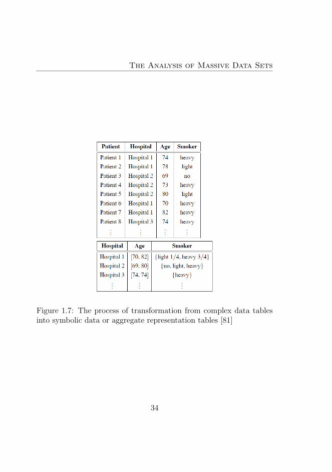
The Analysis of Massive Data Sets
Figure 1.7: The process of transformation from complex data tablesinto symbolic data or aggregate representation tables [81]
34
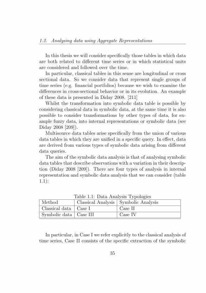
1.2. Analysing data using Aggregate Representations
In this thesis we will consider specifically those tables in which dataare both related to different time series or in which statistical unitsare considered and followed over the time.
In particular, classical tables in this sense are longitudinal or crosssectional data. So we consider data that represent single groups oftime series (e.g. financial portfolios) because we wish to examine thedifferences in cross-sectional behavior or in its evolution. An exampleof these data is presented in Diday 2008. [211]
Whilst the transformation into symbolic data table is possible byconsidering classical data in symbolic data, at the same time it is alsopossible to consider transformations by other types of data, for ex-ample fuzzy data, into internal representations or symbolic data (seeDiday 2008 [209]).
Multisource data tables arise specifically from the union of variousdata tables in which they are unified in a specific query. In effect, dataare derived from various types of symbolic data arising from differentdata queries.
The aim of the symbolic data analysis is that of analysing symbolicdata tables that describe observations with a variation in their descrip-tion (Diday 2008 [209]). There are four types of analysis in internalrepresentation and symbolic data analysis that we can consider (table1.1):
Table 1.1: Data Analysis TypologiesMethod Classical Analysis Symbolic AnalysisClassical data Case I Case IISymbolic data Case III Case IV
In particular, in Case I we refer explicitly to the classical analysis oftime series, Case II consists of the specific extraction of the symbolic
35
The Analysis of Massive Data Sets
descriptions from classical datasets, whereas in Case III symbolic dataare aggregated and transformed into Classical data, and in Case IVit is specifically the case of Symbolic Data Analysis (see Diday 2008[209]).
In this work we will obtain the data as symbolic data and anal-yse these data using the internal representation and a symbolic dataanalysis. In this sense, the present research has produced various sta-tistical methods that could be used in various contexts and situations20
1.3 Aggregate Representations from Time
Series
By considering the case of the time series, various proposals have beenmade: in particular Ferraris Gettler Summa Pardoux and Tong 1995[268] Gettler Summa and Pardoux 2000 [297] and more recently Get-tler Summa et al. 2006 [298] and Gettler Summa, Goldfarb [296] .
The specific steps in an analysis of temporal symbolic data are rep-resented in figure 1.8 and are described in detail in Diday 2008 [209].In particular, for the different stages of a Symbolic Data Analysis seeDiday 1993 [203]:
1. The symbolic data analysis needs to be conducted on two levels:the first level is related to original observations during time t,on the second level are the concepts of the considered temporalintervals.
20For an extensive review of statistical and quantitative methods in SymbolicData Analysis see Diday 2008 [209] and 2011 [214], Diday and Noirhomme 2008[218]. Actual software developments in Symbolic Data Analysis are representedby the Sodas software [743] (see Diday and Noirhomme 2008 [218]) and the recentSyrokko [742]. Various packages in Symbolic Data Analysis are proposed in R.
36
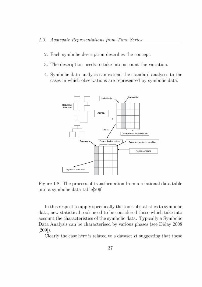
1.3. Aggregate Representations from Time Series
2. Each symbolic description describes the concept.
3. The description needs to take into account the variation.
4. Symbolic data analysis can extend the standard analyses to thecases in which observations are represented by symbolic data.
Figure 1.8: The process of transformation from a relational data tableinto a symbolic data table[209]
In this respect to apply specifically the tools of statistics to symbolicdata, new statistical tools need to be considered those which take intoaccount the characteristics of the symbolic data. Typically a SymbolicData Analysis can be characterised by various phases (see Diday 2008[209]).
Clearly the case here is related to a dataset H suggesting that these
37
The Analysis of Massive Data Sets
data should be handled statistically. In other cases, for example in thedata stream, we consider only the symbolic data as histogram databecause we cannot handle the single observations directly (in this casedata cannot be collected at all: Balzanella Irpino Verde 2010 [56]).We follow this approach:
1. It is assumed to start by considering more than one time series ina specifically built relational database. In this case the classicaldata set is obtained.
2. The series are pre-processed to detect and manage outliers.
3. The series are pre-processed in order to take into account themissing values and the imputation.
4. The specific interval is chosen (by defining a specific query).
5. Overgeneralization is checked (the appropriate symbolic data touse and their appropriate structure are chosen).
6. The symbolic data table is obtained.
1.4 A study simulation on Big Data and
Information Loss
Here we present a simulation study21 considering big datasets andinformation loss in the aggregation process. In particular, we willsimulate various time series models based on a large quantity of data,and we aggregate these data using various aggregation functions (themean and/or the median) for a limited number of periods. At the sametime we compute the interval of the minimum and the maximum in
21See Koenker 1996 [429] for the design of a simulation study
38
1.5. Applications on Real Data
each period. The aggregation is necessary because of the difficultyof visualizing the original time series (we will consider this point indepth in chapter 6). The interval shows clearly the information lossesof each subperiod of i observations. An indicator of information losscould be:
IL =n∑i=1
∣∣xi − xi∣∣ (1.4)
To compare the results between different periods and different ag-gregations some t−test are used. These confirm the result expected. Inparticular: the higher the aggregation interval considered, the higheris the information loss.
1.5 Applications on Real Data
1.5.1 The Symbolic Factorial Conjoint Analysisfor the Evaluation of the Public Goods
The evaluation of the public services is related to a specified set ofdifferent public policy alternatives: Marchitelli 2009 [486] and Dragoet al. 2009 [230].
The aim of the analysis is to compare different policy alternativesthat could be considered competitive. The data coming from evalua-tion procedures are difficult to measure and to model, so to face theproblem of different measurement we need to use representations asintervals.
More precisely the problem can be considered an optimization one,where we want to choose the best alternative with respect to a specificmetric and the budget constraint. The evaluation or the choice needsto take into account the local social development and the environmentof a specific zone or territory. The evaluation can be ex-ante if the
39
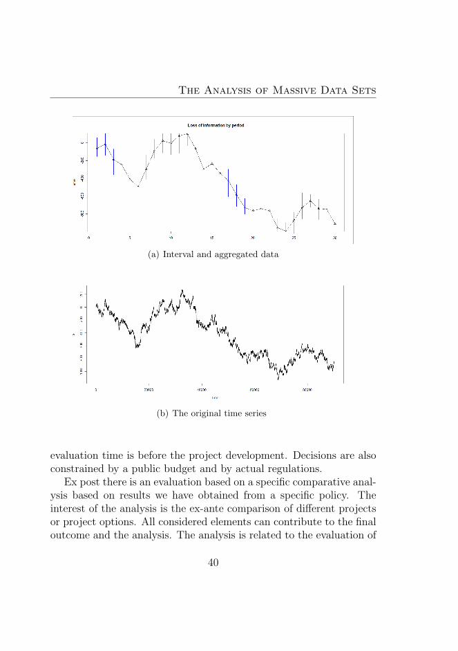
The Analysis of Massive Data Sets
(a) Interval and aggregated data
(b) The original time series
evaluation time is before the project development. Decisions are alsoconstrained by a public budget and by actual regulations.
Ex post there is an evaluation based on a specific comparative anal-ysis based on results we have obtained from a specific policy. Theinterest of the analysis is the ex-ante comparison of different projectsor project options. All considered elements can contribute to the finaloutcome and the analysis. The analysis is related to the evaluation of
40
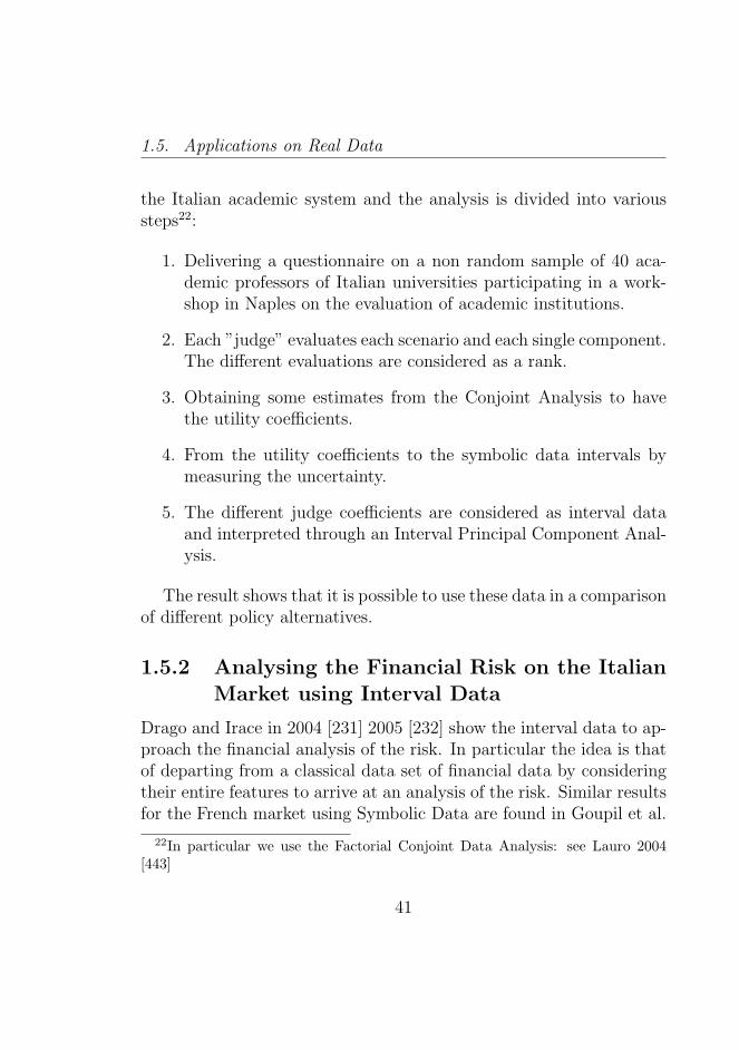
1.5. Applications on Real Data
the Italian academic system and the analysis is divided into varioussteps22:
1. Delivering a questionnaire on a non random sample of 40 aca-demic professors of Italian universities participating in a work-shop in Naples on the evaluation of academic institutions.
2. Each ”judge” evaluates each scenario and each single component.The different evaluations are considered as a rank.
3. Obtaining some estimates from the Conjoint Analysis to havethe utility coefficients.
4. From the utility coefficients to the symbolic data intervals bymeasuring the uncertainty.
5. The different judge coefficients are considered as interval dataand interpreted through an Interval Principal Component Anal-ysis.
The result shows that it is possible to use these data in a comparisonof different policy alternatives.
1.5.2 Analysing the Financial Risk on the ItalianMarket using Interval Data
Drago and Irace in 2004 [231] 2005 [232] show the interval data to ap-proach the financial analysis of the risk. In particular the idea is thatof departing from a classical data set of financial data by consideringtheir entire features to arrive at an analysis of the risk. Similar resultsfor the French market using Symbolic Data are found in Goupil et al.
22In particular we use the Factorial Conjoint Data Analysis: see Lauro 2004[443]
41
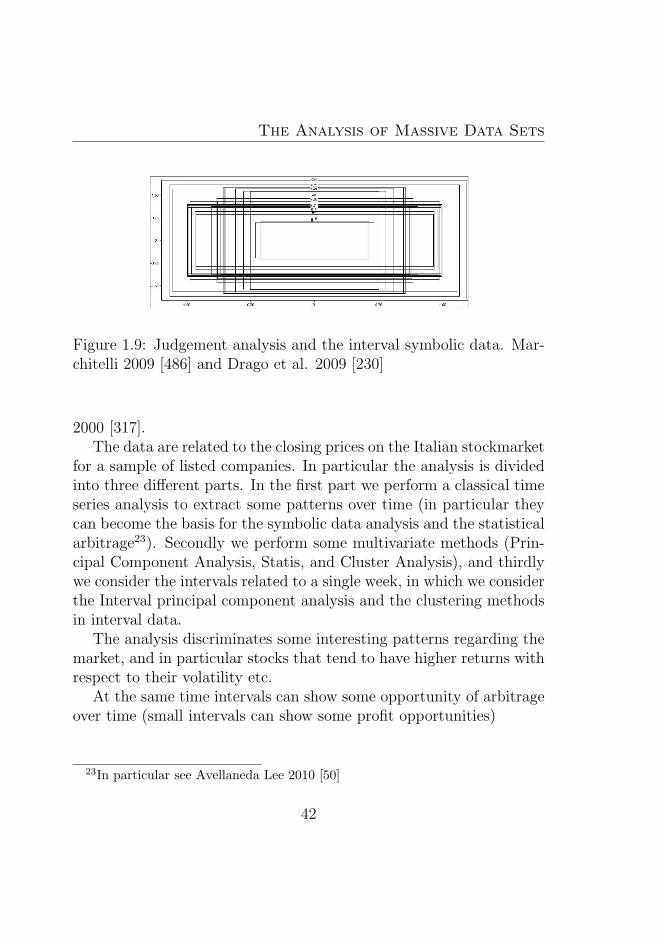
The Analysis of Massive Data Sets
Figure 1.9: Judgement analysis and the interval symbolic data. Mar-chitelli 2009 [486] and Drago et al. 2009 [230]
2000 [317].The data are related to the closing prices on the Italian stockmarket
for a sample of listed companies. In particular the analysis is dividedinto three different parts. In the first part we perform a classical timeseries analysis to extract some patterns over time (in particular theycan become the basis for the symbolic data analysis and the statisticalarbitrage23). Secondly we perform some multivariate methods (Prin-cipal Component Analysis, Statis, and Cluster Analysis), and thirdlywe consider the intervals related to a single week, in which we considerthe Interval principal component analysis and the clustering methodsin interval data.
The analysis discriminates some interesting patterns regarding themarket, and in particular stocks that tend to have higher returns withrespect to their volatility etc.
At the same time intervals can show some opportunity of arbitrageover time (small intervals can show some profit opportunities)
23In particular see Avellaneda Lee 2010 [50]
42
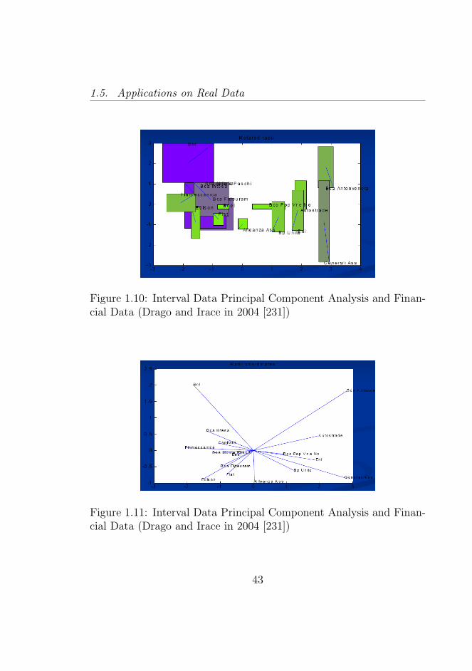
1.5. Applications on Real Data
Figure 1.10: Interval Data Principal Component Analysis and Finan-cial Data (Drago and Irace in 2004 [231])
Figure 1.11: Interval Data Principal Component Analysis and Finan-cial Data (Drago and Irace in 2004 [231])
43
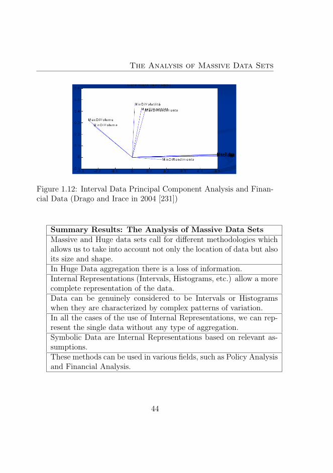
The Analysis of Massive Data Sets
Figure 1.12: Interval Data Principal Component Analysis and Finan-cial Data (Drago and Irace in 2004 [231])
Summary Results: The Analysis of Massive Data SetsMassive and Huge data sets call for different methodologies whichallows us to take into account not only the location of data but alsoits size and shape.In Huge Data aggregation there is a loss of information.Internal Representations (Intervals, Histograms, etc.) allow a morecomplete representation of the data.Data can be genuinely considered to be Intervals or Histogramswhen they are characterized by complex patterns of variation.In all the cases of the use of Internal Representations, we can rep-resent the single data without any type of aggregation.Symbolic Data are Internal Representations based on relevant as-sumptions.These methods can be used in various fields, such as Policy Analysisand Financial Analysis.
44
Chapter 2
Complex Data in aTemporal Framework
The methods described in the thesis, as will be made clear later, canbe applied in various data contexts, one of them being financial. So inthis section we will present the characteristics of the high frequencyfinancial data and at the same time the nature of these time seriesthat call for the use of different methods1.
We will motivate the interest in financial data2 by showing theusefulness of the methods proposed in the thesis, by analysing somecharacteristics of the financial data as a whole and proposing them as
1In particular in recent years there has been a growth of the use of differentmethods for financial data: see Tsay 2005 [667], Campbell Lo and McKinlay 1996[118], Ruppert 2010 [599] Kovalerchuk and Vitayev 2000 [431], Tam Kiang Chi1991 [650] and Mantegna Stanley 2000 [485] on the enormous literature of thequantitative methods in finance
2In particular, we refer to high frequency data that presents some unequal spacecharacteristics which presenting important challenges to operators in the field, see:Dacorogna et al. 2001 [163], but also Zivot 2005 [722], Cont 2011 [154] and alsoBauwens Hautsch 2006 [67]
Complex Data in a Temporal Framework
an initial framework of our methods3 (see the discussion on internaland external modelling and their applications). It is important to noteand underline that the methods can also be used in other frameworksor contexts4.
We analyse data at different frequencies5 because there is no bestinterval temporal in all circumstances and the generating process needsto be analysed (In this approach we follow directly Dacorogna 2001[163].
Here the term ”complex” can be used in two different ways. Thefirst one is in the sense that time series are typically original structureddata coming from different sources (in this sense, see Diday 2010 [211],Diday Noirhomme 2008 [218], but also 2006 [208] and 2002 [207])in which we can obtain some representations which summarize thetemporal observation by retaining the meaning.
In the second meaning the time series could be characterized bysome behaviors like irregular cycles, complex seasonal patterns, nonstationarities, waves, peaks, nonlinearities outliers etc. (see De LiveraHyndman Snyder 2010 [190] Sewell 2008 [619] and Gao Cao TungHu 2007 [290]). In this sense some representations could be useful indetecting the underlying data structure.
In practice, in the complex time series we can assume its structureis hidden from the noise, so it is necessary to separate the ”signal”
3It is important to note that a direct application of the method belongs tohigh frequency financial data for the intrinsic reasons of these data types, see forexample Arroyo et al. 2011 [38] Drago Scepi 2010 [236], Drago Scepi 2010 [237]and Drago Lauro Scepi 2011 [235]
4Original complex data in temporal framework can be adapted to all disciplines,so the methods can be used in different frameworks (see for example Diday 1998[205] on the definition of time series as complex data)
5An interesting methodology is MIDAS (Mixed Data Analysis) considering re-gressions by merging data from different sampling frequencies: Andreou GhyselsKourtellos 2010 [20] and 2010 [21], Ghysels Sinko Valkanov 2007 [303] Ghysels(2005) [301]
46
2.1. Homogeneous and Inhomogeneous Time Series
from the ”noise” to use the data in an improved way. We considerin Chapter 7 an approach to internal representations that takes intoaccount model data, in which we will try to separate in the data thestructural part from the noise6.
2.1 Homogeneous and Inhomogeneous Time
Series
As seen in the first chapter there was an important evolution in finan-cial markets due to the availability of new types of data. In particularin Financial Markets the advances in computer technology and datastorage have made the high frequency data available for researchers(see in this sense Yan Zivot 2003 [710]). In particular, very importantwas the introduction of automated electronic systems of trading thatpermit the transformation into readily available of entire records con-taining the characteristics of all the trades and quotes executed in aregulated market (Galli 2003 [286]).
A typical example is the Trade and Quotes (TAQ) database7 thatprovides a collection of relevant information like prices and quotesfor all the stocks listed on the New York Stock Exchange (NYSE),the American Stock Exchange, the Nasdaq National Market System(NASDAQ), and the SmallCap issues. An example of the final datasetis shown in Galli 2003 [286], see in particular figure.2.1.
So these data refer to time stamped transaction-by-transaction ortick-by-tick data, referred to as ultra-high-frequency data by EngleRussell (2004) [254]. There are known problems in time scales due tothe occurrence of these new types of data (see Mantegna Stanley 2000
6A similar approach is chosen by Signoriello 2008 [630]7See Kyle Obizhaeva Tuzun 2010 [440] for the characteristics of the database
TAQ in trading game contexts
47
Complex Data in a Temporal Framework
[485]). In specific financial contexts the number of observations in highfrequency data sets can be overwhelming and data are often recordedwith errors and there is a need for it to be cleaned and corrected priorto direct analysis.
Transaction by transaction data on trades and quotes are, by na-ture, irregularly spaced time series with random daily numbers of ob-servations. High-frequency data typically exhibit periodic intra-dayand intra-week patterns in market activity. In these cases the needfor aggregation arises. In particular there is the need for techniquesto summarize, visualize, cluster and forecast high frequency financialtime series without information loss. At the same time, the need tostudy the financial market as a whole using multivariate tools andcointegrated time series where all data are high frequency data (thereis no mix of different frequencies) is essential.
2.1.1 Equispaced Homogeneous Data
A scalar time series8 yt can be represented along the notion of scalarstochastic process9. Following Peracchi (2001) [555]: on the spaceΩ×T can be defined a function Z as a scalar stochastic process, suchthat a random variable is defined on the probability space (Ω, A, P )for every t ∈ T , Z(−, t).10
Assuming a common probability space (Ω, A, P ) a scalar stochasticprocess is a collection Z(., t), t ∈ T ) of random variables, a state
8In this thesis, we consider various types of time series, for example the scalarone (STS), but at the same time, interval time series (ITS), boxplot time series(BoTS), histogram time series (HTS) etc. See in this sense Arroyo, Gonzalez-Rivera, Mate, San Roque (2011) [38] Arroyo Gonzalez-Rivera Mate (2010) [41],Han Hong Wang (2009) [336]
9Ross 1996 [596] and Dobb 1953 [223]. Interval stochastic processes are definedin Han Hong Wang 2009 [336]
10Peracchi 2001 [555]
48
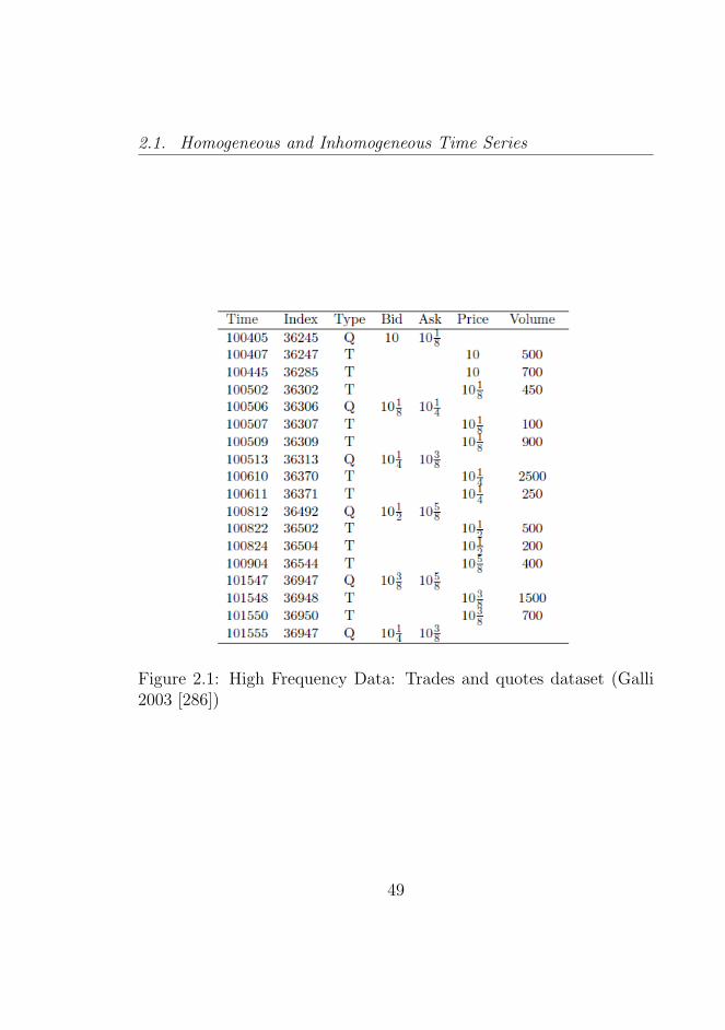
2.1. Homogeneous and Inhomogeneous Time Series
Figure 2.1: High Frequency Data: Trades and quotes dataset (Galli2003 [286])
49
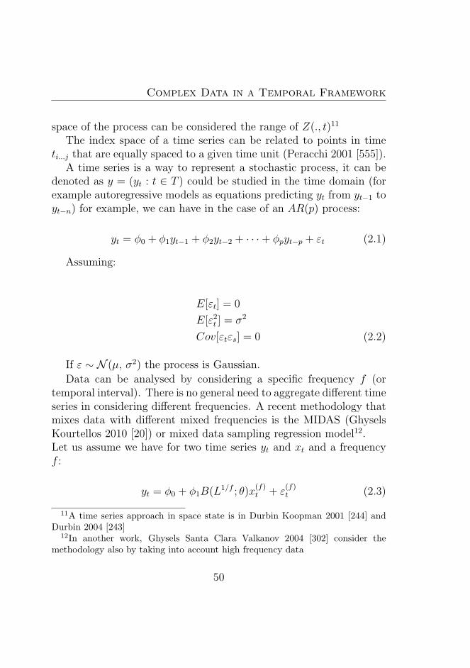
Complex Data in a Temporal Framework
space of the process can be considered the range of Z(., t)11
The index space of a time series can be related to points in timeti...j that are equally spaced to a given time unit (Peracchi 2001 [555]).
A time series is a way to represent a stochastic process, it can bedenoted as y = (yt : t ∈ T ) could be studied in the time domain (forexample autoregressive models as equations predicting yt from yt−1 toyt−n) for example, we can have in the case of an AR(p) process:
yt = φ0 + φ1yt−1 + φ2yt−2 + · · ·+ φpyt−p + εt (2.1)
Assuming:
E[εt] = 0
E[ε2t ] = σ2
Cov[εtεs] = 0 (2.2)
If ε ∼ N (µ, σ2) the process is Gaussian.
Data can be analysed by considering a specific frequency f (ortemporal interval). There is no general need to aggregate different timeseries in considering different frequencies. A recent methodology thatmixes data with different mixed frequencies is the MIDAS (GhyselsKourtellos 2010 [20]) or mixed data sampling regression model12.Let us assume we have for two time series yt and xt and a frequencyf :
yt = φ0 + φ1B(L1/f ; θ)x(f)t + ε
(f)t (2.3)
11A time series approach in space state is in Durbin Koopman 2001 [244] andDurbin 2004 [243]
12In another work, Ghysels Santa Clara Valkanov 2004 [302] consider themethodology also by taking into account high frequency data
50
2.1. Homogeneous and Inhomogeneous Time Series
In practice f denotes the frequency (daily, weekly, quarterly) ,B(L1/f )is a lag distribution (for example, the Almon Lag). We start by con-sidering the characteristics of high frequency data compared with eq-uispaced homogeneous data.
A time series could be analysed, also, in the frequency domain(harmonic analysis, periodogram analysis and spectral analysis: seeBattaglia 2007 [66]).
Box and Jenkins 1970 [99] show that the time-domain and the fre-quency domain show equivalent information on the time series13.
An important distinction needs to be made, in financial data inparticular, by considering the spacing of the data points in time. Reg-ularly spaced time series are usually defined as homogeneous whilstirregularly spaced are defined inhomogeneous (we use here the termi-nology in Dacorogna 2001 [163]). In the second case, we cannot applystandard methods that are designed for regularly spaced or homoge-neous time series data14
In relation to the homogeneous time series we consider the finitetime series xt with length T and N observations. In the case of pe-riodic sampling, the temporal distance between two realizations is al-ways constant (Ng 2006 [535] and Zumbach Muller 2001 [726])
In fact, by considering ti and tj as single observations we have ti−tjrelating to the distance between two different observations, we have15:
t− tj = ∆t =1
T∀j ∈ N (2.4)
13An interesting review is proposed in Warner (1998) [693] focusing in particularon spectral analysis. A simple introduction to these methods is given by Brandeset al. (1968) [108]
14See Hamilton 1994 [333], Lutkepohl 2005 [469], Battaglia 2007 [66]15Ng 2008 [536]
51
Complex Data in a Temporal Framework
Ng 2006 [535] and in 2008 [536]16 shows that the time original ho-mogeneous time series can be considered as a sum of trigonometricpolynomials.
yt =
N/2−1∑o=−N/2
ao cos(2πot) + bo sin(2πot)
=
N/2−1∑o=−N/2
co exp−i2πot/N (2.5)
In this case, the Fourier Coefficients can be computed by the FastFourier Transforms (also denoted as FFT).17.
co =1
N
N∑t=1
xt exp−i2πot/N (2.6)
High frequency transaction data arrives in irregular time intervals,the implementation of the common FFT cannot be done for the un-evenly sampled data (Ng 2006 [535]).
In the case of the high frequency data we can consider the PointProcess, we will consider it later (for a complete introduction to thePoint Processes see Karr 1991 [418] and Daley Vere-Jones (1988)[165]).
2.1.2 Inhomogeneous High Frequency Data
High Frequency financial data are typically inhomogeneous. Manytypes of financial data can be obtained at high frequency, intraday
16See also Fricks 2007 [281]17For a presentation of these methods see Percival Walden 2006 [556]
52
2.1. Homogeneous and Inhomogeneous Time Series
specifically, at a market tick by tick frequency. There are cases inwhich raw data are not suitable: in these cases market ticks arrive inrandom times. Engle (2000) [250], Zumbach and Muller (2001) [726]and more recently Zivot and Yang (2006) [723] deal directly with ir-regularly spaced data.In that sense, following Zumbach and Muller (2001) [726] xi is definedas an inhomogeneous time series. Here the market transactions overtime can be characterized as (ti, zi). In that sense ti is the time andzi is the scalar, representing, for example a price. So zi = z(ti) andthe point ti are the i − th element of the series. More specifically aninhomogeneous time series is denoted as (zi)
Ni .
In practice a time series x is defined by the arrival of ticks zi attimes ti. Over time ti+1 > tt. As we know, homogeneous time seriesare regularly spaced, inhomogenous time series are irregularly sampledti+1 − tt 6= ∆t (Muller 1996 [520]).
Various methods can be considered for obtaining homogeneous timeseries from inhomogeneous (Dacorogna 2001 [163] Zumbach and Muller(2001) [726] and also Brownlees and Gallo 2006 [115]).
By starting with an inhomogeneous series with times ti followingDacorogna 2001 [163], we have a transformation from inhomogeneousto homogenous time series zi = zti . In practice only the last obser-vation in the time is chosen. The sequence of the raw series can berelated to the index i while in the case of the homogeneous we considerthem at time t. By considering a specific period ∆t we obtain a series:t0 + i∆t regularly spaced.
The ticks xi indexed, each related to the market characteristics (seein figure 2.1 price and volume in particular) for each index i can beconsidered as the realizations of a marked point processes.
In particular, we can consider the different partitions of the TAQdataset as a specific high frequency dataset, here we need to considerseparately the Trades and the Quotes.
For trades tr considering i = 1...n as the number of the trades over
53
Complex Data in a Temporal Framework
time we have (tr1i, tr2i, tr3i), with tr1i as the time of the trade tr2i asthe price and tr3i as the volume.
For quotes qu, considering the number j = 1...n at the same timewe have (qu1j, qu2j, qu3j) we have: qu1j for the time qu2j as the bidprice qu3j as the ask price (see Galli 2003) [286]. So Trade Durationdata, in fig.2.2, can be finally defined:
Di = tr1i − tr1(i−1) (2.7)
Where we can define at the same time the Quote duration data(fig.2.3):
Qj = tr1j − tr1(j−1) (2.8)
These types of data can be analyzed by considering specific econo-metric methods, such as the ACD or Autoregressive Conditional Du-ration models18 (see Engle and Russell, 1998 see [253] and Engle2000 [250]). In practice we model the durations between two distinctevents19
durationi = tri − tri−1 (2.9)
2.1.3 Irregularly Spaced Data as Point Processes
High Frequency Data present the particular characteristics of beinginhomogeneous or irregularly spaced. In Statistics we define this typeof process as a Point Process. In particular, a Point Process is arandom element, whose values are in a defined set S. The outcome
18See also the interesting comparison between methods in Zhang Keasey andCai [718]
19Forecasting the arrival of an event is clearly relevant in various other applica-tive contexts. See for example the forecasting methodology and its application inShen and Huang 2008 [625]
54
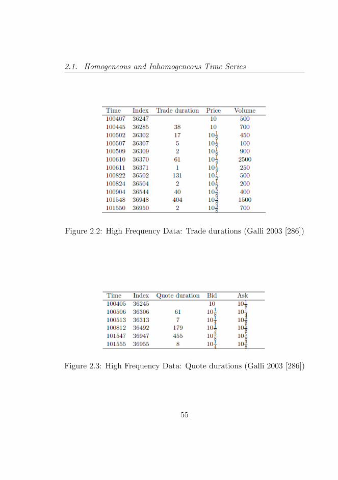
2.1. Homogeneous and Inhomogeneous Time Series
Figure 2.2: High Frequency Data: Trade durations (Galli 2003 [286])
Figure 2.3: High Frequency Data: Quote durations (Galli 2003 [286])
55
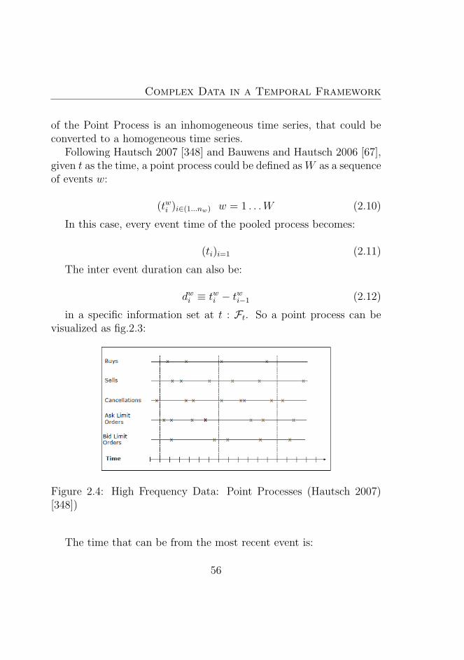
Complex Data in a Temporal Framework
of the Point Process is an inhomogeneous time series, that could beconverted to a homogeneous time series.
Following Hautsch 2007 [348] and Bauwens and Hautsch 2006 [67],given t as the time, a point process could be defined as W as a sequenceof events w:
(twi )i∈(1...nw) w = 1 . . .W (2.10)
In this case, every event time of the pooled process becomes:
(ti)i=1 (2.11)
The inter event duration can also be:
dwi ≡ twi − twi−1 (2.12)
in a specific information set at t : Ft. So a point process can bevisualized as fig.2.3:
Figure 2.4: High Frequency Data: Point Processes (Hautsch 2007)[348])
The time that can be from the most recent event is:
56
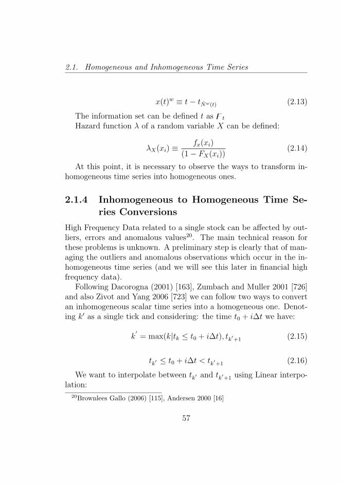
2.1. Homogeneous and Inhomogeneous Time Series
x(t)w ≡ t− tNw(t) (2.13)
The information set can be defined t as zt
Hazard function λ of a random variable X can be defined:
λX(xi) ≡fx(xi)
(1− FX(xi))(2.14)
At this point, it is necessary to observe the ways to transform in-homogeneous time series into homogeneous ones.
2.1.4 Inhomogeneous to Homogeneous Time Se-ries Conversions
High Frequency Data related to a single stock can be affected by out-liers, errors and anomalous values20. The main technical reason forthese problems is unknown. A preliminary step is clearly that of man-aging the outliers and anomalous observations which occur in the in-homogeneous time series (and we will see this later in financial highfrequency data).
Following Dacorogna (2001) [163], Zumbach and Muller 2001 [726]and also Zivot and Yang 2006 [723] we can follow two ways to convertan inhomogeneous scalar time series into a homogeneous one. Denot-ing k′ as a single tick and considering: the time t0 + i∆t we have:
k′= max(k|tk ≤ t0 + i∆t), tk′+1 (2.15)
tk′ ≤ t0 + i∆t < tk′+1 (2.16)
We want to interpolate between tk′ and tk′+1 using Linear interpo-lation:
20Brownlees Gallo (2006) [115], Andersen 2000 [16]
57
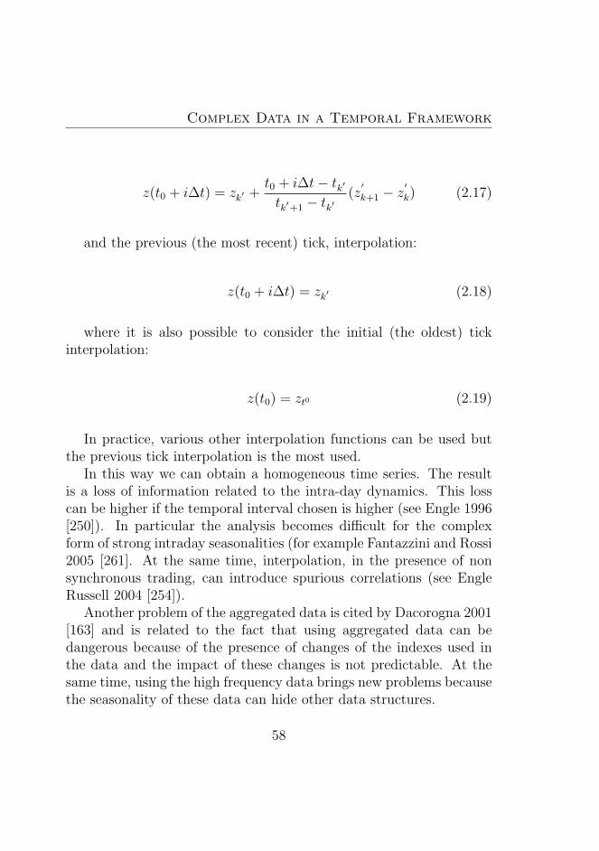
Complex Data in a Temporal Framework
z(t0 + i∆t) = zk′ +t0 + i∆t− tk′tk′+1 − tk′
(z′
k+1 − z′
k) (2.17)
and the previous (the most recent) tick, interpolation:
z(t0 + i∆t) = zk′ (2.18)
where it is also possible to consider the initial (the oldest) tickinterpolation:
z(t0) = zt0 (2.19)
In practice, various other interpolation functions can be used butthe previous tick interpolation is the most used.
In this way we can obtain a homogeneous time series. The resultis a loss of information related to the intra-day dynamics. This losscan be higher if the temporal interval chosen is higher (see Engle 1996[250]). In particular the analysis becomes difficult for the complexform of strong intraday seasonalities (for example Fantazzini and Rossi2005 [261]. At the same time, interpolation, in the presence of nonsynchronous trading, can introduce spurious correlations (see EngleRussell 2004 [254]).
Another problem of the aggregated data is cited by Dacorogna 2001[163] and is related to the fact that using aggregated data can bedangerous because of the presence of changes of the indexes used inthe data and the impact of these changes is not predictable. At thesame time, using the high frequency data brings new problems becausethe seasonality of these data can hide other data structures.
58
2.2. Ultra High Frequency Data Characteristics
2.2 Ultra High Frequency Data Charac-
teristics
In recent years there has been an increase of the availability of higherfrequency measurements of the economy. This fact has been very pos-itive because it has made for the improvement of the likelihood of thestatistical analysis21. It is important to note that the limit of thisprocess can be reached when all the transactions have been recordedand this could happen in different markets. In this sense, each marketcan generate transactions, so data could be collected in the same timetick by tick (or observation by observation) by considering differentproducts in the market locations such as supermarkets, internet, orfinancial markets, see Engle 2000 [250].
So, high frequency data, as inhomogeneous time series, are increas-ingly important in financial markets. They allow us to study theadjustment processes of prices in the financial markets, the intradaydynamics and the market microstructure (for the mechanisms in whichthe new information impact on price see for example Cont 2011 [154]and Engle Russell 2004 [254]22. High-frequency data are also usefulfor analysing, at a lower frequency, the volatility of asset returns andfor portfolio allocation23. At the same time, just as the high frequencydata has fuelled advanced forms of algorithmic trading so has the highfrequency trading, based on these data24.The first set of characteristics we will analyse in depth is: irregulartemporal spacing (as a characterising difference with other types of
21See for example Modugno 2011 [511]22In particular the relationships between ”order flow, liquidity and price dynam-
ics” in Cont (2011) [154]. See also Bouchaud Mezard Potters 2002 [104] Farmer etal. 2004 [264]
23Corsi, Dacorogna, Muller, Zumbach (2001) [159], Barucci Reno (2002) [61]and Hautsch Kyj Malec (2011) [349]
24Ahmed M. 2009 [10] and Patterson Rogow 2009[552]
59
Complex Data in a Temporal Framework
financial data at a daily or weekly frequency), diurnal patterns, pricediscretness, and very long dependence (Engle Russell 2004 [254], Da-corogna 2001 [163]).
Another important reason is to understand how the financial mi-crostructure can affect price dynamics25.
It is important to note that the institutional regulations that collectthe information on markets (also defined as the market microstructure)can change data characteristics. Changes in market regulations andtechnological advances modify the data characteristics and the differ-ent data structures. For an example of this variability over the timeand the space of the data characteristics see Brownlees and Gallo 2006[115].
2.2.1 Overwhelming number of observations
Size refers to the number of ticks in a specific trading day. The high-frequency databases storing tick-by-tick data are very complex to ana-lyze, for example Brownlees, Gallo 2006 [115]. The first characteristicfor the high frequency financial datasets is that they are of an over-whelming size.
The transmission by data vendors can vary from market to market,for example Reuters for a foreign exchange spot rate distributes morethan 75,000 prices per day (see Dacorogna 2001 [163]). In other cases,the datasets size can be over 10 million foreign exchange price quotes(Dacorogna Muller Pictet De Vries 2001 [164]).
Clearly the different sizes of the data sets depend on the differentmarkets26. Mykland and Zhang (2009) [525] cite the fact that on a
25Cont (2011) [154] Biais, Glosten, Spatt (2005) [79] and Rosu 2009 [597]26For an example of the specific characteristics of high frequency data for ex-
change rates see Dacorogna et al. 1993 [162] and 1990 [161]. Dacorogna MullerPictet De Vries 2001 [164] study the exchange rates focusing on the outliers andthe heavy tail features of foreign exchange returns. The authors found at the
60
2.2. Ultra High Frequency Data Characteristics
single day Merck had 6,302 transactions and Microsoft had 80,982. Ingeneral, we can conclude that the size is very relevant.At the same time, the number of ticks, or observations, produced canvary greatly considering the different markets and different financialinstruments. A “highly traded stock may have tens of thousands ofprice events per day, quickly resulting in a storage requirement to storeGigabytes of data per day and Terabytes of data per year for any rea-sonable sized instrument universe”(Xenomorph 2007 [706]).
Engle and Russell confirm that these data “are characterized byten thousands of transactions or posted quotes in a single day timestamped to the nearest second” [254]27.
It is important to note that if the data volume is growing exponen-tially so at the same time the storage of the intraday or high frequencydata is becoming difficult28.
This type of characteristic neglects for example to visualize cor-rectly the data and it is necessary to consider distinct windows forobserving all data29 (see Drago and Scepi [237]).
2.2.2 Gaps and erroneous observations in data
High Frequency datasets contain gaps and wrong observations, andsome unordered sequences30. At the same time, Brownlees and Gallo2006 [115] report that these data can be characterized by some anoma-lous and occasional behavior determined by specific market conditions(opening, closing, trading halts, for example). In particular, the 2-
same time that high frequency data improve the efficiency of the tail risk cum lossestimates
27see also Yang Zivot 2003 [711] and Falkenberry 2002 [260]28See in the specialized journal Automatic Trader the interview of Brian Sen-
tance (2007) [732]29Zivot 2005 [722]30Yang Zivot 2003 [711]
61
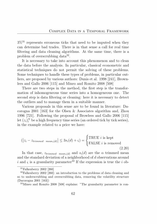
Complex Data in a Temporal Framework
3%31 represents erroneous ticks that need to be imputed when theycan determine bad trades. There is in that sense a call for real timefiltering and data cleaning algorithms. At the same time, there is aproblem of overscrubbing data32.
It is necessary to take into account this phenomenon and to cleanthe data before the analysis. In particular, classical econometric andstatistical techniques do not permit the solving of these problems.Some techniques to handle these types of problems, in particular out-liers, are proposed by various authors: Dunis et al. 1998 [241], Brown-lees and Gallo 2006 [115] and Mineo and Romito 2008 [508]
There are two steps in the method, the first step is the transfor-mation of inhomogeneous time series into a homogeneous one. Thesecond step is data filtering or cleaning: here it is necessary to detectthe outliers and to manage them in a suitable manner.
Various proposals in this sense are to be found in literature: Da-corogna 2001 [163] for the Olsen & Associates algorithm and, Zhou1996 [721]. Following the proposal of Browlees and Gallo 2006 [115]let (zi)
Ni be a high frequency time series (an ordered tick by tick series),
in the example related to a price we have:
(∣∣zi − ztrimmed meani(d)
∣∣ ≤ 3si(d) + ς) =
TRUE i is kept
FALSE i is removed
(2.20)In that case, ztrimmed meani(d) and si(d) are the α trimmed mean
and the standard deviation of a neighborhood of d observations aroundi and ς is a granularity parameter33 If the expression is true the i ob-
31Falkenberry 2002 [260]32Falkenberry 2002 [260]: an introduction to the problems of data cleaning and
so to underscrubbing and overscrubbing data, removing the volatility structure(Dacorogna 2001 [163])
33Mineo and Romito 2008 [508] explains: ”The granularity parameter is con-
62
2.2. Ultra High Frequency Data Characteristics
servation is kept, if the expression is false the i observation is declaredan outlier and it is removed.
Mineo and Romito 2008 [508] make a proposal in this sense:
(|zi − zmeani(d)| ≤ 3s−i(d) + ς) =
TRUE i is kept
FALSE i is removed(2.21)
In that case zmeani(d) and s−i(d) are the mean and the standarddeviation of a neighborhood of d observations around i without thei−th observation and ς is the granularity parameter. A third approachconsidered in Dunis (2008) is related to the median of the last threeticks34
In this sense, the outliers are detected and removed from the data.For a specific guide to the data analysis preparation and variable cre-ation see Yang Zivot 2003 [711]. See in figure 2.5 and figure 2.6 someexamples of erroneous observations in high frequency data.
2.2.3 Price discreteness
There are important features in high frequency data that determinesome spurious auto-correlations in data, for example, the price dis-creteness35. The price discreteness in the high frequency data is re-lated to the high kurtosis manifested from data36.
Price discreteness can be considered to be the truncation of prices
sidered because the ultra high-frequency series often contains sequences of equalprices which would lead to a zero variance; thus, it is useful to introduce a lowerpositive bound on price variation in order to have always admissible solutions.
34Mineo and Romito 2008 [508] report that the Dunis method performs withthe worst performance in respect to other methods used
35Matei 2011 [495]36Dacorogna 2001 [163] and Engle Russell 2004 [254]
63
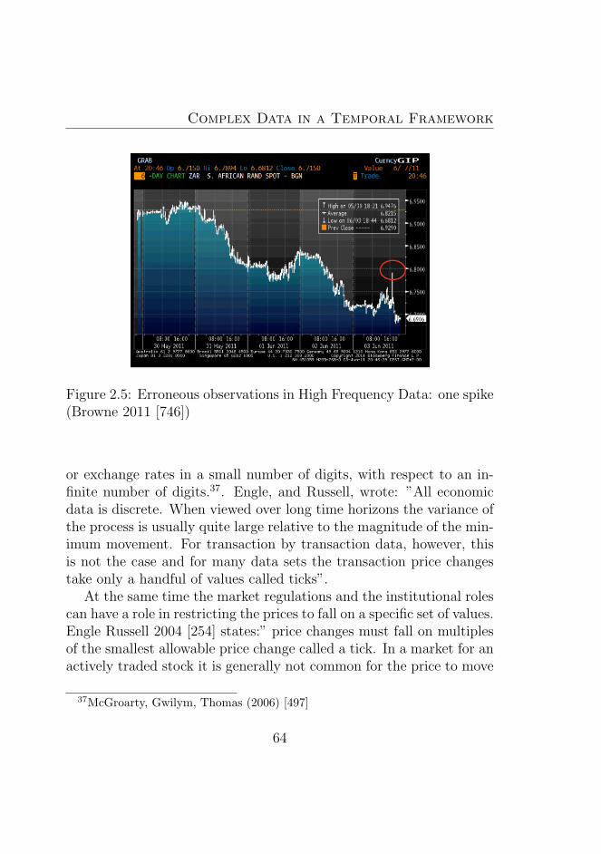
Complex Data in a Temporal Framework
Figure 2.5: Erroneous observations in High Frequency Data: one spike(Browne 2011 [746])
or exchange rates in a small number of digits, with respect to an in-finite number of digits.37. Engle, and Russell, wrote: ”All economicdata is discrete. When viewed over long time horizons the variance ofthe process is usually quite large relative to the magnitude of the min-imum movement. For transaction by transaction data, however, thisis not the case and for many data sets the transaction price changestake only a handful of values called ticks”.
At the same time the market regulations and the institutional rolescan have a role in restricting the prices to fall on a specific set of values.Engle Russell 2004 [254] states:” price changes must fall on multiplesof the smallest allowable price change called a tick. In a market for anactively traded stock it is generally not common for the price to move
37McGroarty, Gwilym, Thomas (2006) [497]
64
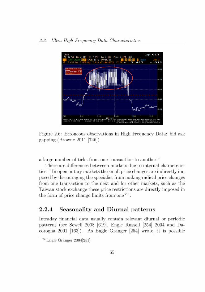
2.2. Ultra High Frequency Data Characteristics
Figure 2.6: Erroneous observations in High Frequency Data: bid askgapping (Browne 2011 [746])
a large number of ticks from one transaction to another.”There are differences betweeen markets due to internal characteris-
tics: ”In open outcry markets the small price changes are indirectly im-posed by discouraging the specialist from making radical price changesfrom one transaction to the next and for other markets, such as theTaiwan stock exchange these price restrictions are directly imposed inthe form of price change limits from one38”.
2.2.4 Seasonality and Diurnal patterns
Intraday financial data usually contain relevant diurnal or periodicpatterns (see Sewell 2008 [619], Engle Russell [254] 2004 and Da-corogna 2001 [163]). As Engle Granger [254] wrote, it is possible
38Engle Granger 2004[251]
65
Complex Data in a Temporal Framework
to detect a U-shaped pattern over the day, for most stock markets,volatility, the frequency of trades, volume, and spreads show a U-shaped pattern.
These patterns need to be considered before beginning any statis-tical inference on the data39. In that sense, it is important to explorethe data to detect the pattern of seasonality in data.
In any case, various different patterns can be detected in the mar-kets40 and they can be determined by complex relations, for examplewith market microstructure or the public arrival of information.
These patterns are clearly different from the patterns we are ableto extract in financial data at a lower frequency, as for example, thewell known ”January effects” 41. In these cases we can define them aseffects due to to market anomalies that challenge the idea of perfectefficiency in the financial markets. In any case, the idea of data struc-tures and different patterns in different types of data is confirmed byconsidering different data frequencies42.
2.2.5 Long dependence over time
Following the approach of the data characteristics of Engle and Rus-sell 2006 [254] related to the market structures, the authors refer tovarious phenomena: the existence of a long dependence over time isone of the most important.
The dependence can be considered the result of price discretenessand the spread between the price paid by buyer and seller initiatedtrades. Long dependence can be referred to as bid-ask bounce and thelarge first order negative autocorrelation.
39Melvin Yin (2000) [503] Andersen and Bollerslev (1994) [17] and Dacorogna,et.al (1993) [162]
40Kunst 2007 [439]41Keim 1983 [420]42Dacorogna 2001 [163]
66
2.2. Ultra High Frequency Data Characteristics
Traders breaking large orders up into a sequence of smaller ordersin the hope of transacting at a better price overall can lead to a depen-dence in price changes. These buys and sells, so sequentially ordered,can determine a sequence of transactions that change prices in thesame direction.
Hence, on long term horizons we sometimes find positive autocor-relations. This result is confirmed in many studies of intra day data43
2.2.6 Distributional characteristics and ExtremeRisks
See Dacorogna 2001 [163]. Distributional characteristics change withrespect to the frequency, the more frequent the data the more thedata share high frequency characteristics, the more the distributionsare fat tailed. The general result for the distribution is that the dataare fat tailed [163] and also characterized by strong skewness [261].In general, by considering the choice of little intervals of time for theconversion to inhomogeneous time series of homogeneous ones (forexample 15 minutes) the distribution chosen is leptokurtic (see alsothe nonparametric approach in Coroneo Veredas (2006) [157].
The presence of high frequency data allows for the good analysisof fat tails. From the applicative point of view it is interesting toanalyse the tails to understand the extreme movements in the financialmarkets. The Extreme Risk analysis is a growing area in the field ofFinancial Econometrics (see Cont 2001 [152]).
2.2.7 Scaling Laws
At the same time scaling laws are present in financial data at differentfrequencies (see in particular Dacorogna 2001 [163] and Sewell 2008
43Sun Rachev Fabozzi 2007 [646]
67
Complex Data in a Temporal Framework
[619]). Following Sewell 2011 [621] who reviews the characteristics ofthe financial time series ”Scaling laws describe the absolute size ofreturns as a function of the time interval at which they are measured.Markets exhibit non-trivial scaling properties”.
At the same, Sewell in two works in 2011 [761] and [621], reviewsvarious different contexts in which it is possible to find scaling laws infinance irrespective of underlying data or frequency.
So, there now exists a vast empirical verification from that of theinitial work of Muller et al. 1990 [520] which found the existence ofscaling laws in financial data like the FX rates (see Dacorogna 2001[163]). The evidence was confirmed also by considering other marketsusing different financial instruments.
2.2.8 Volume, Order Books and Market Microstruc-ture
The dynamics of the volumes, order books, and market microstruc-ture, seem to be relevant in understanding how markets work in real-ity. At the same time, the market functioning, market institutions andmarket processes impact on trading costs, prices, volume and tradingbehaviour (see Sewell 2008 [619] but also Tsay 2005 [667]).In particular, Tsay 2005 [667] refers to High-frequency data as a keyto understanding some characteristics useful in analysing and under-standing some phenomena like:
1. Nonsynchronous trading
2. Bid-ask spread
3. Duration models
4. Price movements that are in multiples of tick size
68
2.2. Ultra High Frequency Data Characteristics
5. Bivariate models for price changes
6. Time durations between transactions associated with price changes
In general, the advantage of using high frequency data gives thepossibility of investigating the concrete elements that relate to thedeterminants of the adjustment price.
High frequency data can be very relevant in the analysis of thedifferent trading processes in various markets related to the marketmicrostructure. In particular (see Tsay 2005 [667]) they can be usedto compare the efficiency of the trading systems in price discovery.The analysis of market efficiency can be carried out by consideringhigh frequency data44.
The use of the high frequency data is important, here, for the resultsthat are new in respect to the low frequencies.
2.2.9 Volatility Clustering
Similarly to financial data at lower frequencies we can observe thevolatility clustering phenomenon at higher frequencies.
In particular, we can take into account the seasonal heteroskedas-ticity by considering the daily and the weekly clusters of volatility (seeDacorogna 2001 [163]).
In any case, this observation allows us to investigate if we can ob-serve the same data characteristics in different data frequencies. Now,considering the data at a different frequency (a lower one) we investi-gate its specific characteristics45.
44Lillo 2010 [456] Tiozzo 2011 [659]45Sewell 2011 [621]
69
Complex Data in a Temporal Framework
2.3 Financial Data Stylized Facts
Whereas High Frequency Data are a new data type, that promise toenlighten various phenomena on the financial markets, the classicalway to consider financial data is a lower frequency (daily and weeklydata).
On the general characteristics of the financial data at a lower fre-quency (days) there is a growing literature based on the so calledstylized facts (see Sewell 2008 [619], Cont 2001 [152], Tsay 2005 [667]also in the new field of the Econophysics Mantegna and Stanley 2000[485] ).
Here we focus on the statistical characteristics of the financial timeseries. There are two types of series that are generally used: priceseries pft at a given frequency f and return series rft . pft can be con-sidered as the price of a financial item, for example an asset, and theln(pt) as its logarithm transformation, useful for many purposes46.The rft , with respect to pft shows useful statistical properties, so it iswidely used, in particular we have (see Tsay 2005 [667]) the simplegross return:
1 + rft =pft
pft−1
(2.22)
or also
pft = pft − 1(1 + rft ). (2.23)
The simple net return is:
rft =pft
pft−1
− 1 =pft − p
ft−1
pft−1
= r(t, T ) (2.24)
46See Lutkepohl Xu 2009 [471]
70
2.3. Financial Data Stylized Facts
Following Cont (2001) [152], and generalizing for different temporalscales in a defined time scale ∆t, that could be considered as a secondor a month in a homogeneous time series, the log return at scale ∆twill be:
rt,∆t = xt+∆t − xt (2.25)
By considering the returns of a portfolio q of assets l with weightsαi on the different assets, given the simple return of an asset rfl,t, wecan define the simple return of the portfolio q, at time t as:
rfq,t =N∑i=1
αirfi,t (2.26)
See Tsay (2005) [667].
2.3.1 Random Walk Models and Martingale Hy-pothesis
A relevant hypothesis used in an important class of financial data (theprices) is the Random Walk and the Martingale Hypothesis. By follow-ing Tsay (2005) [667] Samuelson (1965) [605] and Mantegna Stanley(2000) [485] and Campbell Lo MacKinlay Lo (1996) [118] in general,the hypothesis of market efficiency is related to the pft+1 the price as
the past values pf0 , pf1 , . . . , p
ft through the conditions:
E(pft+1 | pft , p
ft−1, . . . ) = pft (2.27)
E(pft−1 − pft | p
ft , p
ft−1, ...) = 0 (2.28)
Stochastic processes like these are defined martingales. There is nopossibility for making profits. The concept is linked with the randomwalk price model, given by:
71
Complex Data in a Temporal Framework
pft+1 = pft + ηt (2.29)
It is not possible to forecast the difference pt−pt−1 so the best pre-diction for pt+s is pt (see Nakamura Small 2007 for the tests associatedwith the Random Walk Hypothesis [528]). A Random Walk with driftbecame:
pft = pft−1 + β + ηt (2.30)
where an upward trend appears considering β > 0.
pft = pf0 + βt+n∑t=1
ηt (2.31)
p0 + βt is the deterministic trend, where∑n
t=1 ηt is the stochastictrend. For the properties see Mantegna and Stanley 2000 [485]. In theweak form of the market efficiency there is no simple way to use pastinformation in order to gain a profit. Financial data show a complexstructure because they convey a large quantity of mechanisms thatoverlap in the influence of the series, the objective is to separate theinformation that is possible to predict, that could be evidence thatmarkets are not completely efficient (see Mantegna and Stanley 2000[485]).
One objective for the representation considered during the thesis isto discover some useful structures, both for the high frequency dataand the classical financial data. In this sense, these market inefficien-cies could be exploited (until the markets recover efficiency). For a listof market inefficiencies see Sewell 2008 [619], Lo and MacKinlay 1999[466] and for the contrary opinion see Malkiel 1973 [481]. In recentyears many financial models have used data sources as high frequencydata (see Dacorogna 2001 [163]).
72
2.3. Financial Data Stylized Facts
2.3.2 Distributional Properties of Returns: FatTails
Cont (2001) [152], defined the joint distribution of the returns asr(t, T ) The unconditional distribution of returns can be defined aswell as:
FT (u) = P (r(t, T ) ≤ u) (2.32)
The kurtosis can indicate the deviation from the normal distribu-tion:
κ =r(t, T )− (r(t, T ))4
σ(T )4− 3 (2.33)
where σ(T )4 is the variance of the log returns r(t, T ) = x(t+ T )−x(t). The kurtosis is defined such that κ = 0 for a Gaussian dis-tribution, a positive value of κ indicating the fat tail, or the slowasymptotic decay of the PDF. In this way it is possible to take intoaccount the risk. Cont (2001) [152] defines the Value-at-Risk (VaR)as a ”high quantile of the loss distribution of a portfolio over a certaintime horizon”:
P (W0(r(t,∆)− 1) ≤ V aR(p, t,∆)) = p (2.34)
Where W0 is the present market value of the portfolio, r(t,∆t)its (random) return between t and t+ ∆t . ∆t is typically taken to
be one day or ten days and p = 1% or 5%
2.3.3 Heterogeneity and Structural Changes
We follow the characterization of the financial time series proposed bySewell (2011) [621]. In that sense, financial returns r(t, T ) are typi-
73
Complex Data in a Temporal Framework
cally non stationary47. In fact the standard deviation of the returnstend to be not stationary over time. Following Mantegna and Stanley2000 [485] the same volatility on markets is time dependent.
Financial data shows frequent structural changes. This result is co-herent with the idea that the structural changes need to be approachedin the analysis using different time windows for forecasting or mod-elling using the data (see Pesaran and Timmermann 2004 [558]). Mar-kets are continously changing so parameter drifts in the models canoccur frequently.In general the ARCH (Engle 1982 [249]) and GARCH (Bollerslev [102]1986) models for returns r(t, T ), frequently used in finance are nonstationary in variance but not in mean 48. At the same time astructural change occurs in a given defined statistical model, for ex-ample:
pft = β + βtf + εt, t = 1 . . . T (2.35)
with εt ∼ iidN(0, σ2) No structural change parameters α = 1.2 andβ = 1 Structural change β = 2 for t > 150
Various tests in the literature exist to detect the existence of struc-tural change in financial data. The best known are the Chow Forecasttest (Chow 1960 [140]) and also the CUSUM and CUSUMSQ Tests(Brown Durbin Evans 1975 [114]).
2.3.4 Non-Linearity
Various types of nonlinearity can be detected in financial stock returnsr(t, T ). Sewell in his work [621] reviews the results in literature re-lated to the phenomenon. Financial markets show not only frequent
47Sewell (2011) [621], for a different approach Starica and Granger 2005 [640]De Lima 1998 [181]
48Sewell 2008 [619]
74
2.3. Financial Data Stylized Facts
structural changes but at the same form some predictable forms ofnonlinearities (see Lim Brooks Hinich 2008 [457]).
Typically the time series models can be non linear in mean and orin variance (as the ARCH or GARCH models)49.
2.3.5 Scaling
Scaling can be defined as a relation between time intervals t and theaverage volatility measured at a power η of the absolute returns ob-served (Sewell 2008 [619]). From the first work of Mandelbrot in 1963[482] that found scaling, in cotton prices pt, various other works havefound scaling in financial data50. It is possible to confirm the same ob-servations seen in paragraph 2.2.7 on scaling laws related to the highfrequency financial data. In that sense, it is possible to conclude thata predefinite data frequency for this financial time series characteristicdoes not exist.
2.3.6 Dependence and Long Memory
Following Cont 2001 [152] and Sewell 2008 [619].If time lags are denoted as τ : the correlation between the different
lags s becomes:
corr[r(s+ τ,∆t), r(s,∆t)] (2.36)
By assuming the hypothesis of ”market efficiency” (the ”efficiencymarket hypothesis” depicted in 2.3.1) then it can be hypothesized thatthere is no autocorrelation of the returns r(t, T ).
In any case the ”market efficiency” hypothesis seems to be toostrong in some markets and some ”market inefficiencies” can appear
49Engle 1982 [249] and Bollerslev 1986 [102]50Sewell 2011 [621]
75
Complex Data in a Temporal Framework
(and their use is a matter of empirical investigation51). Some exam-ples in literature of autocorrelation of returns can be found in Sewell2011 [619].
A different phenomenon is the Long Memory dependence of dailystock return series. In this case, the evidence (for returns, volatil-ity, volume etc.) is mixed by using the R/S Statistic, also known as”rescaled range” or ”range over standard deviation” from Hurst 1951[374]. Clearly a Hurst Exponent value (or R/S statistic) related tothe:
H(0.5 < H < 1) (2.37)
can suggest an inefficiency in the considered market52 (where wecan identify a long memory process).
Following Cont 2001 [152] given a time scale ∆ the log return ofthe scale ∆ is given by rt = Xt+∆ −Xt = ln(St+∆
St)
A stationary process Yt (with finite variance) is said to have longrange dependence if its autocorrelation function C(τ) = corr(Yt), Yt+τdecays as a power of the lag τ 53 : C(τ) = corr(Yt, Yt+τ )τ→∞ ∼L(τ))τ1−2d 0 < d < 1
2
2.3.7 Volatility Clustering
The phenomenon of volatility clustering, is related to the fact thatin financial time series: ”large changes tend to be followed by largechanges, of either sign, and small changes tend to be followed by smallchanges” (Mandelbrot 1963 [482]).
The phenomenon are usually considered by taking into account theARCH and GARCH models, in which volatility is related to the last
51Lo Mackinlay 1999 [466]52Peters 1996 [560]53Cont 2001 [152]
76
2.3. Financial Data Stylized Facts
period volatility (period of calm on markets followed by periods ofturbulence).
2.3.8 Chaos
Chaos can be defined (Sewell 2008 [619]) when it is possible to detectin data an unpredictable long term behavior that could be generatedby some sensitive initial conditions in a deterministic dynamical sys-tem. In practive the behavior of a chaotic time series is usually nondistinguishable from another stochastic time series (Barnett SalmonKirman (eds.) 1996 [60]).
Sewell in 2011 [621], reviews various works that test the existenceof chaos in data by concluding that there is little empirical evidencein financial markets of low-dimensional chaos.
2.3.9 Cross Correlations Between Assets
To understand the correlation between assets see Cont 2001 [152] andTsay 2005 [667].
In particular, it is very important to consider the problems when wedeal with many assets. In various financial applications and problems(for example portfolio asset allocation and risk management) it is veryrelevant to work not only with single assets.
In this sense, the joint distribution of the returns of the assets needto be known in order to conduct a statistical analysis of these data:Cont 2001 [152]. An important outcome in these types of analyses isthe understanding of the contagion mechanisms of different stocks (ormarkets) in the crises. These types of correlations vary over time andspace.
77
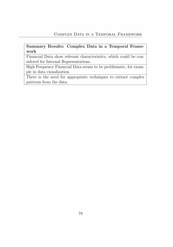
Complex Data in a Temporal Framework
Summary Results: Complex Data in a Temporal Frame-workFinancial Data show relevant characteristics, which could be con-sidered for Internal Representations.High Frequency Financial Data seems to be problematic, for exam-ple in data visualization.There is the need for appropriate techniques to extract complexpatterns from the data.
78
Chapter 3
Foundations of IntervalsData Representations
We have seen in Chapters 1 and 2 that sometimes Internal Repre-sentations can be useful in retaining information from overwhelmingdatasets. That is, it is useful to consider the entire data structure orthe entire distribution of the data.1 In that sense, the existent litera-ture in Data Analysis using Internal Representation of big data2 usesmainly two classes of approaches: a first one using Interval data (anal-ysed in this chapter) and a second one using Histogram and or Boxplot
1See in Williamson 1989 [701] ”If one looks at the development of the mea-surement process during the past century one soon observes that with increasingfrequency the raw data are probability distribution functions or frequency func-tions rather than real numbers This is so in the physical sciences and in the bio-logical and social sciences it is the rule rather than the exception. One may thusconvincingly argue that distribution functions are the numbers of the future andthat one should therefore study these new numbers and their arithmetic (BertholdSchweizer)”.
2For example the literature in Symbolic Data Analysis, see in that sense Billard2010 [82] and Diday Noirhomme 2008 [218]
Foundations of Intervals Data Representations
data (analysed in Chapter 4)3. In the recent past there has been anevolution using other instruments, based on different approaches. InChapter 5 we propose a new method of analysis of big data based onKernel Density Estimation. At the same time, it is relevant to notethat this chapter could be a mathematical foundation of the densitiesas internal representation. The densities or the beanplot we will lookat in Chapter 5 use upper and lower bounds to understand relevantphenomena. So this chapter starts with the mathematical foundationsof the internal representations (IR).
We stress that these representations can be genuine4 or can comefrom previous statistical processes that transform the initial data ma-trix into representation matrices5. At times we can obtain our originaldata as intervals, histograms etc. The classical data type is used whentaking into account the imprecision6, the interval is useful to considera range of different values in temporal aggregations in the interval. Inthis chapter the foundations of the interval analysis and its algebra,and the interval random variables, are presented. Starting from thisit is possible to develop the interval stochastic processes and inter-val time series (ITS). In the next chapter we symmetrically developthe theory for the boxplots and the histogram data (another repre-sentation). In any event it is important to start from probabilisticarithmetic (Williamson 1989 [701]) that can be considered relevant in
3A general foundation of these approaches can be found in the imprecision andthe vagueness, some data can be measured considering uncertainty (or risk) and socan be considered intervals, boxplots, histograms etc. to measure such uncertainty.See for an introduction to this approach: Palumbo (2011) [544]
4In that case there can be a specific interpretation of these data that couldbe found in Nature. An example is temperature with its range of minimum andmaximum-considered a genuine interval data
5For example interval data can come from database queries see for exampleDiday 2002 [206]
6See for example in Gioia 2008 [309] the classification of error that could befound in data and in their solutions
80
3.1. Internal Representation Data and Algebra: intervals
order to understand the interval data (or the upper and lower boundof the density data).
3.1 Internal Representation Data and Al-
gebra: intervals
3.1.1 Probabilistic Arithmetic
The idea in Williamson 1989 [701] is to calculate the distribution ofarithmetic functions of random variables. In some cases the resultsare obtained in terms of dependency bounds (for example, in the caseof the lower and upper bounds). In practice, the probabilistic arith-metic is a generalization of interval arithmetic that considers only thesupports of the distributions of the variables7. The problem adressed8
is given by considering Z = L(X, Y ) with X and Y as independentrandom variables, where its distribution function is FX,Y . The distri-bution FZ function of Z could be written:
FZ(z) =
∫L(z)
d(FX(u)FY (v)), (3.1)
where: L(z) = ((u, v) | u, v ∈ <, L(u, v) < z). The author statesthat to compute the expression is a necessary but not a sufficientcondition for a probabilistic arithmetic. The dependency error canbe defined as the error in computing the distribution of some func-tion of V and W (U = V/W ) assuming V and W are independent.For example X, Y and Z are assumed independent random variables,but V = X + Y or W = X × Z are not necessarily independent.
7Williamson 1989 [701]8We refer on Williamson 1989 [701]
81
Foundations of Intervals Data Representations
Williamson 1989 [701] states that is possible to obtain partial solu-tions to these problems in terms of dependency bounds or the lowerand upper bounds on the distributions of functions of random vari-ables when only the marginal distributions are known. So we have:ldb and udb as lower and upper dependency bounds, where is abinary operation, it is possible to write the bounds:
ldb(FX , FY ,)(z) ≤ FZ(z) ≤ udb(Fx, Fy,)(z) (3.2)
At the same time the general approach has been studied by var-ious authors. Springer 1979 [637]9 considers the idea of an algebraof random variables to calculate the convolutions. Various authorshave also studied the numerical methods for calculating distributionsof functions of random variables10. In the case of interval data we aremore interested in the bounds of a distribution within an interval.
3.1.2 Interval Data and Algebra
In particular, Interval Data are the simplest and used means to repre-sent both the intra-period and the measurement error or imprecision.
Various contributions11 have appeared from the original work ofSunaga 1958 [647], and Moore 1962 [512] and 1966 [513]. At the sametime, interval data and interval arithmetic found a relevant applicationobtaining reliable simulation mechanisms, see in this sense Batarseh
9The idea was applied in Downs Cook Rogers 1984 [226]10Williamson 1989 [701] in particular in the Chapter 211Gioia 2008 [309] reviews the different approach in Interval Algebra from the
first contributors: Burkill 1924 [117], Young 1931 [712], Warmus 1956 [691] thenSunaga 1958 [647] and Warmus 1961 [692] . At the same time, modern approachesby Moore 1966 [513], Alefeld-Herzerberger 1983 [12], Kerarfott-Kreinovich 1996[423], Neumaier 1990 [533], and Alefeld-Mayer 2000 [13], Hickey Ju Van Emden2001 [360]. For the latest works in interval algebra see Kreinovich 2011 [755]
82
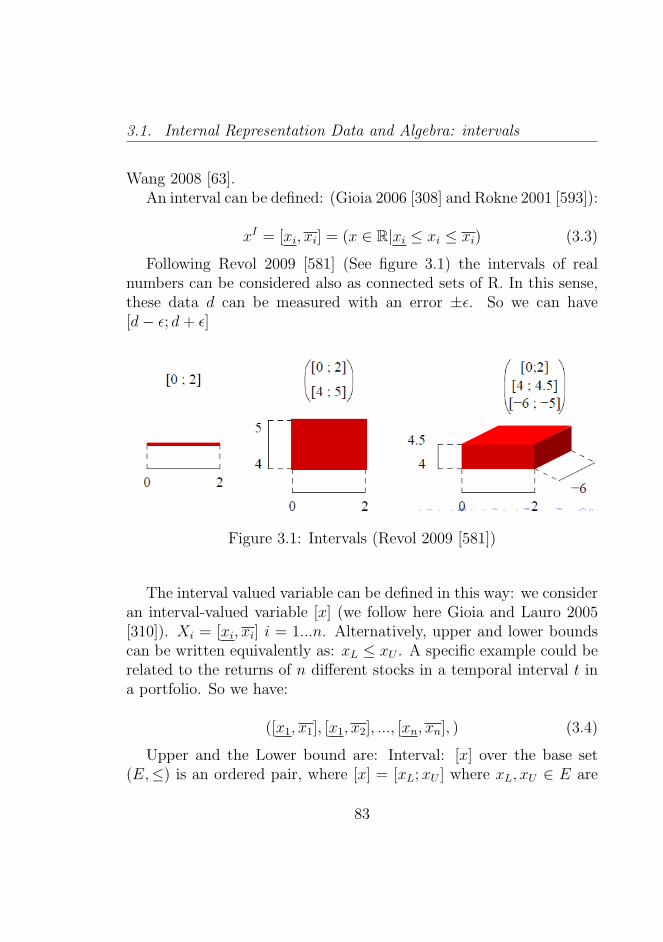
3.1. Internal Representation Data and Algebra: intervals
Wang 2008 [63].An interval can be defined: (Gioia 2006 [308] and Rokne 2001 [593]):
xI = [xi, xi] = (x ∈ R|xi ≤ xi ≤ xi) (3.3)
Following Revol 2009 [581] (See figure 3.1) the intervals of realnumbers can be considered also as connected sets of R. In this sense,these data d can be measured with an error ±ε. So we can have[d− ε; d+ ε]
Figure 3.1: Intervals (Revol 2009 [581])
The interval valued variable can be defined in this way: we consideran interval-valued variable [x] (we follow here Gioia and Lauro 2005[310]). Xi = [xi, xi] i = 1...n. Alternatively, upper and lower boundscan be written equivalently as: xL ≤ xU . A specific example could berelated to the returns of n different stocks in a temporal interval t ina portfolio. So we have:
([x1, x1], [x1, x2], ..., [xn, xn], ) (3.4)
Upper and the Lower bound are: Interval: [x] over the base set(E,≤) is an ordered pair, where [x] = [xL;xU ] where xL, xU ∈ E are
83
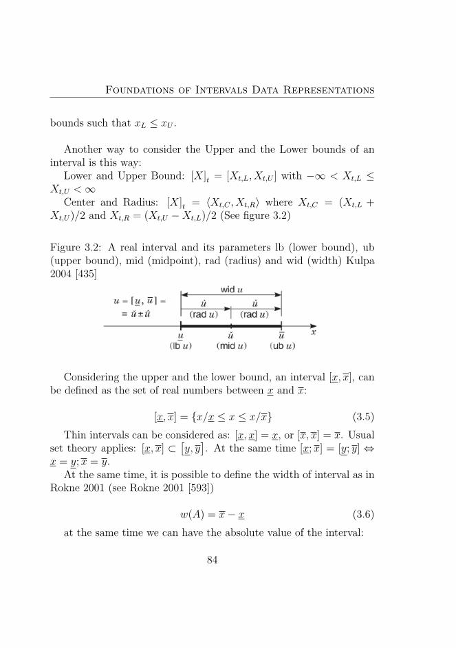
Foundations of Intervals Data Representations
bounds such that xL ≤ xU .
Another way to consider the Upper and the Lower bounds of aninterval is this way:
Lower and Upper Bound: [X]t = [Xt,L, Xt,U ] with −∞ < Xt,L ≤Xt,U <∞
Center and Radius: [X]t = 〈Xt,C , Xt,R〉 where Xt,C = (Xt,L +Xt,U)/2 and Xt,R = (Xt,U −Xt,L)/2 (See figure 3.2)
Figure 3.2: A real interval and its parameters lb (lower bound), ub(upper bound), mid (midpoint), rad (radius) and wid (width) Kulpa2004 [435]
Considering the upper and the lower bound, an interval [x, x], canbe defined as the set of real numbers between x and x:
[x, x] = x/x ≤ x ≤ x/x (3.5)
Thin intervals can be considered as: [x, x] = x, or [x, x] = x. Usualset theory applies: [x, x] ⊂
[y, y]. At the same time [x;x] = [y; y] ⇔
x = y;x = y.At the same time, it is possible to define the width of interval as in
Rokne 2001 (see Rokne 2001 [593])
w(A) = x− x (3.6)
at the same time we can have the absolute value of the interval:
84
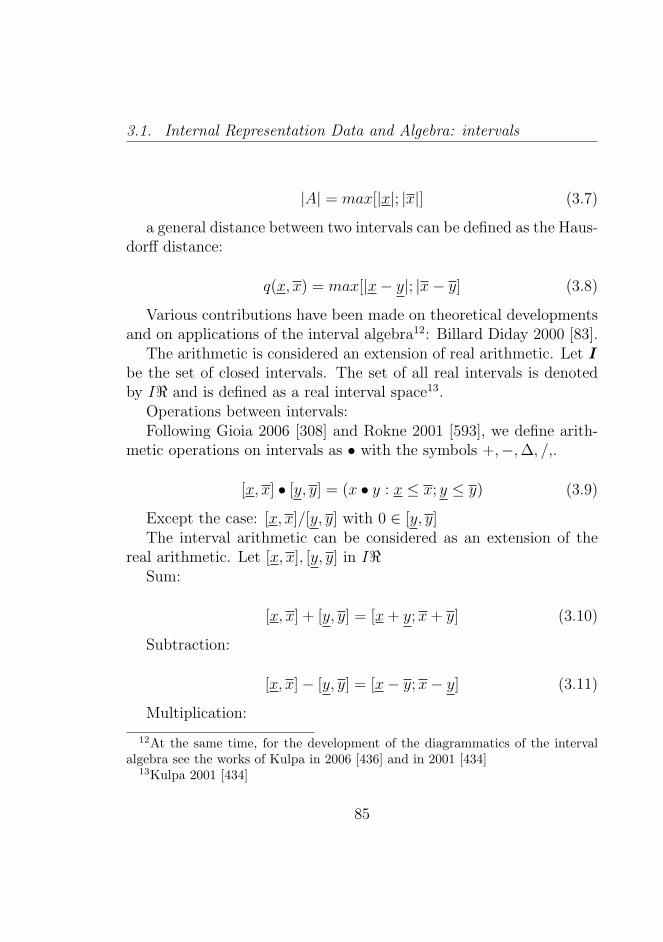
3.1. Internal Representation Data and Algebra: intervals
|A| = max[|x|; |x|] (3.7)
a general distance between two intervals can be defined as the Haus-dorff distance:
q(x, x) = max[|x− y|; |x− y] (3.8)
Various contributions have been made on theoretical developmentsand on applications of the interval algebra12: Billard Diday 2000 [83].
The arithmetic is considered an extension of real arithmetic. Let Ibe the set of closed intervals. The set of all real intervals is denotedby I< and is defined as a real interval space13.
Operations between intervals:Following Gioia 2006 [308] and Rokne 2001 [593], we define arith-
metic operations on intervals as • with the symbols +,−,∆, /,.
[x, x] • [y, y] = (x • y : x ≤ x; y ≤ y) (3.9)
Except the case: [x, x]/[y, y] with 0 ∈ [y, y]The interval arithmetic can be considered as an extension of the
real arithmetic. Let [x, x], [y, y] in I<Sum:
[x, x] + [y, y] = [x+ y;x+ y] (3.10)
Subtraction:
[x, x]− [y, y] = [x− y;x− y] (3.11)
Multiplication:
12At the same time, for the development of the diagrammatics of the intervalalgebra see the works of Kulpa in 2006 [436] and in 2001 [434]
13Kulpa 2001 [434]
85
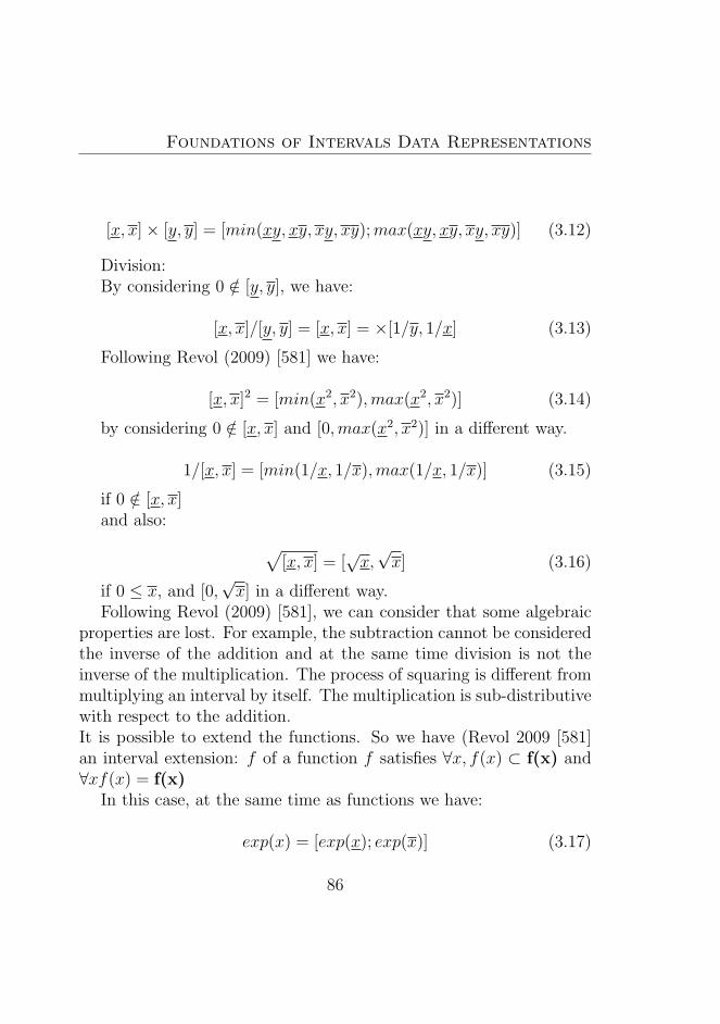
Foundations of Intervals Data Representations
[x, x]× [y, y] = [min(xy, xy, xy, xy);max(xy, xy, xy, xy)] (3.12)
Division:By considering 0 /∈ [y, y], we have:
[x, x]/[y, y] = [x, x] = ×[1/y, 1/x] (3.13)
Following Revol (2009) [581] we have:
[x, x]2 = [min(x2, x2),max(x2, x2)] (3.14)
by considering 0 /∈ [x, x] and [0,max(x2, x2)] in a different way.
1/[x, x] = [min(1/x, 1/x),max(1/x, 1/x)] (3.15)
if 0 /∈ [x, x]and also: √
[x, x] = [√x,√x] (3.16)
if 0 ≤ x, and [0,√x] in a different way.
Following Revol (2009) [581], we can consider that some algebraicproperties are lost. For example, the subtraction cannot be consideredthe inverse of the addition and at the same time division is not theinverse of the multiplication. The process of squaring is different frommultiplying an interval by itself. The multiplication is sub-distributivewith respect to the addition.It is possible to extend the functions. So we have (Revol 2009 [581]an interval extension: f of a function f satisfies ∀x, f(x) ⊂ f(x) and∀xf(x) = f(x)
In this case, at the same time as functions we have:
exp(x) = [exp(x); exp(x)] (3.17)
86
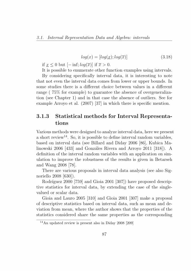
3.1. Internal Representation Data and Algebra: intervals
log(x) = [log(x); log(x)] (3.18)
if x ≤ 0 but [− inf; log(x)] if x > 0.It is possible to enumerate other function examples using intervals.By considering specifically interval data, it is interesting to note
that not even the interval data comes from lower or upper bounds. Insome studies there is a different choice between values in a differentrange ( 75% for example) to guarantee the absence of overgeneraliza-tion (see Chapter 1) and in that case the absence of outliers. See forexample Arroyo et al. (2007) [37] in which there is specific mention.
3.1.3 Statistical methods for Interval Representa-tions
Various methods were designed to analyze interval data, here we presenta short review14. So, it is possible to define interval random variables,based on interval data (see Billard and Diday 2006 [86], Kubica Ma-linowski 2006 [433] and Gonzales Rivera and Arroyo 2011 [318]). Adefinition of the interval random variables with an application on sim-ulation to improve the robustness of the results is given in Betarsehand Wang 2008 [78].
There are various proposals in interval data analysis (see also Sig-noriello 2008 [630]).
Rodrıguez 2000 [759] and Gioia 2001 [307]) have proposed descrip-tive statistics for interval data, by extending the case of the single-valued or scalar data.
Gioia and Lauro 2005 [310] and Gioia 2001 [307] make a proposalof descriptive statistics based on interval data, such as mean and de-viation from mean, where the author shows that the properties of thestatistics considered share the same properties as the corresponding
14An updated review is present also in Diday 2008 [209]
87
Foundations of Intervals Data Representations
statistics for single-valued data (Signoriello 2008) [630]).The general approach for the advanced statistical methods is to con-sider statistical methods for scalar or single-valued data and extendthem for the interval data15.
The extension of the Principal component analysis to interval data(from the scalar data) is developed in various scientific works: start-ing from radii or vertices (see Vertices Principal Components Analysis(also defined as V-PCA) in Cazes et al. 1997 [124]) and a SymbolicObjects PCA (see Lauro Palumbo 2000 [446]) to the considered mid-points (for example the Midpoint and the Radii PCA in Palumbo 2003[543]). Irpino 2006 [393] considers an extension of the classical Prin-cipal Component Analysis to analyse time dependent interval data.Finally, Lauro Verde and Irpino in 2008 [450] review the PrincipalComponent Analysis techniques using interval data.
Signorello 2008 [630] and Palumbo [543] report an important prob-lem in interval algebra (related to the extension of the scalar or single-value data to interval data): ”unfortunately, the interval algebra wasborn in the field of error-theory where intervals are very small, butthis is no longer true for Statistical Interval. First of all the so-calledwrapping effect leads to wider intervals than they actually should be.This effect induces a distinction between “interval of solutions” andthe “interval solutions” .
It is not possible here to present all the works that extend the scalaror single-valued data statistical techniques, for an updated review seeDiday, Noirhomme (2008) [218].
15Signoriello 2008 [630]
88
3.1. Internal Representation Data and Algebra: intervals
3.1.4 Stochastic Processes and Time Series of Interval-Valued Representations
There is a growing literature in Interval Data and Interval Time Series(ITS). In fact, in recent years there has been a literature that considersmore in depth the methods of forecasting using these types of represen-tations. A first contribution is in Teles and Brito (2005) [654], a usefulpaper is that of Cheung who introduces the forecasting of daily highsand lows [133]16, at the same time Maia, De Carvalho and Ludermir in2006 and in 2008 [477] [476] introduce various methods in forecastingintervals, in particular hybrid methods. Different forecasting meth-ods using interval data are considered in Arroyo, Munoz San Roque,Mate , and Sarabıa (2007) [37], in particular exponential smoothing,Arroyo Gonzales Rivera and Mate 2010 [41] on VAR and KNN meth-ods applied in interval forecasting17. Mate and Garcıa Ascanio (2010)[494] compare different forecasting methods (VAR and Neural Net-works) using energy data whereas Arroyo Espınola and Mate (2010)[36] consider financial data in the method comparison.
Another very important paper that develops methods for intervaltime series (ITS) is: Han, Hong and Wang (2009) [336]. An applicationon exchange rates is in Han Hong Lai Wang 2008 [337] and He Hong anWang 2011 [351] with an application on crude oil prices. Forecastingcombinations with interval data is the topic of the work of Salish andRodrigues 2010 [603]18 .
16This paper is particularly important because it introduces some useful methodsused in forecasting intervals. See also Chou who introduces CARR models forvolatility modelling (Chou 2005 [135]), Rogers and Satchell 1991 [592] Spurginand Schneeweis 1999 [638] and Parkinson 1980 [548]
17The distance for interval data are presented in Arroyo Mate 2006 [43]18The author in another work in 2010 and 2011 found evidence of nonlinearity
in financial interval time series (ITS) [602] and [591]
89

Foundations of Intervals Data Representations
Summary Results: IntervalsThe simplest Internal Representation.Assume data to be a Mixture of Uniforms.Interval Algebra as extension of the rules of Arithmetic Algebra.Interval Algebra can be considered to be the foundation of the otherRepresentations.Upper, Lower Bound, Centres and Radii can be descriptors, andcan be considered over time with Attribute Time Series.
90
Chapter 4
Foundations of Boxplots andHistograms DataRepresentations
In this chapter we deal with density valued data methods and theiralgebra. We have seen in the Third Chapter representation character-ized only by two relevant measures (the upper and the lower bound,or the centre and the radius). We have seen that this representationcould be very important if we are interested in extreme values of anaggregate data in preserving some of the original data structure or theinitial distribution (in practice, we are assuming that data follows auniform distribution). In any event, we shall see in this chapter and inChapter 5 that this representation could be improved by consideringother types of representations like the boxplots or the histograms, andfinally in Chapter 5 the densities.
At the same time in this chapter we will make for the first time thedistinction between original data and model data to take into accountthe measurement model that could be determined by various factors.Finally in Chapter 7 we will show how to estimate the coefficients of
Foundations of Boxplots and Histograms DataRepresentations
these data.
4.1 Internal Representation Data and Al-
gebra: Boxplots, Histograms and Mod-
els
4.1.1 Quantile Data and Algebra
In particular there was some debate on the interval arithmetics becausethere were some relevant cases in which interval is not so useful in rep-resenting some variables. Williamson 1989 [701] speaks of a ”numberof techniques which determine limited information about the distribu-tion of functions of random variables”.
At the same time, following Williamson 1989 [701] the general aimis to provide information on the distribution of the variable for theinternal representations, and in this respect it is necessary to considersome types of generalizations of the interval algebra we have alreadylooked at. Various attempts have been made in this sense, Williamson1989 [701], in practice cites two approaches: Triplex Arithmetic andthe Quantile Arithmetic.The problem related to Ecker and Ratschek (1972) [245] as explainedin Williamson (1989) [701] is that they “have considered intervals prob-abilistically in an attempt to understand the phenomena of subdis-tributivity and inclusion monotonicity. They also suggested a jointrepresentation of distributions and intervals and studied some prop-erties of Dempster quantile arithmetic which we examine below”. Atthe same time Williamson (1989) [701] says, about the approach ofAhmad 1975 [9]: “Ahmad is supposed by Moore 1979 [514] to havelooked at the arithmetic of probability distributions from the pointof view of interval arithmetic. However Ahmad’s paper is solely con-
92
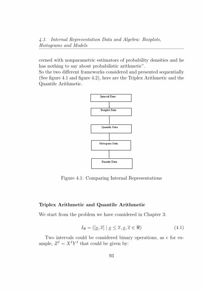
4.1. Internal Representation Data and Algebra: Boxplots,Histograms and Models
cerned with nonparametric estimators of probability densities and hehas nothing to say about probabilistic arithmetic”.So the two different frameworks considered and presented sequentially(See figure 4.1 and figure 4.2), here are the Triplex Arithmetic and theQuantile Arithmetic.
Figure 4.1: Comparing Internal Representations
Triplex Arithmetic and Quantile Arithmetic
We start from the problem we have considered in Chapter 3:
I< = ([x, x] | x ≤ x, x, x ∈ <) (4.1)
Two intervals could be considered binary operations, as c for ex-ample, ZI = XIY I that could be given by:
93
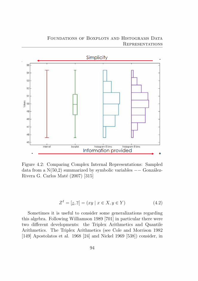
Foundations of Boxplots and Histograms DataRepresentations
Figure 4.2: Comparing Complex Internal Representations: Sampleddata from a N(50,2) summarized by symbolic variables −− Gonzalez-Rivera G. Carlos Mate (2007) [315]
ZI = [z, z] = (xy | x ∈ X, y ∈ Y ) (4.2)
Sometimes it is useful to consider some generalizations regardingthis algebra. Following Williamson 1989 [701] in particular there weretwo different developments: the Triplex Arithmetics and QuantileArithmetics. The Triplex Arithmetics (see Cole and Morrison 1982[149] Apostolatos et al. 1968 [24] and Nickel 1969 [538]) consider, in
94
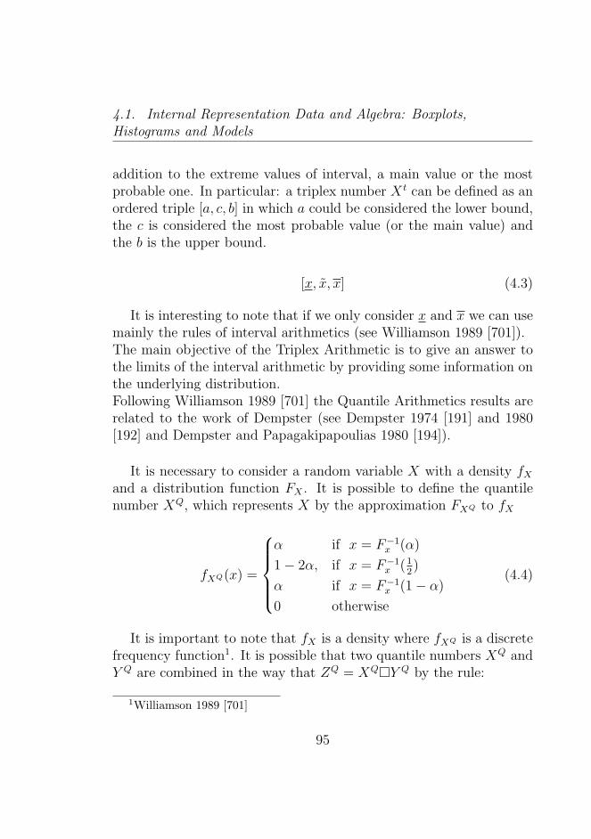
4.1. Internal Representation Data and Algebra: Boxplots,Histograms and Models
addition to the extreme values of interval, a main value or the mostprobable one. In particular: a triplex number X t can be defined as anordered triple [a, c, b] in which a could be considered the lower bound,the c is considered the most probable value (or the main value) andthe b is the upper bound.
[x, x, x] (4.3)
It is interesting to note that if we only consider x and x we can usemainly the rules of interval arithmetics (see Williamson 1989 [701]).The main objective of the Triplex Arithmetic is to give an answer tothe limits of the interval arithmetic by providing some information onthe underlying distribution.Following Williamson 1989 [701] the Quantile Arithmetics results arerelated to the work of Dempster (see Dempster 1974 [191] and 1980[192] and Dempster and Papagakipapoulias 1980 [194]).
It is necessary to consider a random variable X with a density fXand a distribution function FX . It is possible to define the quantilenumber XQ, which represents X by the approximation FXQ to fX
fXQ(x) =
α if x = F−1
x (α)
1− 2α, if x = F−1x (1
2)
α if x = F−1x (1− α)
0 otherwise
(4.4)
It is important to note that fX is a density where fXQ is a discretefrequency function1. It is possible that two quantile numbers XQ andY Q are combined in the way that ZQ = XQY Q by the rule:
1Williamson 1989 [701]
95
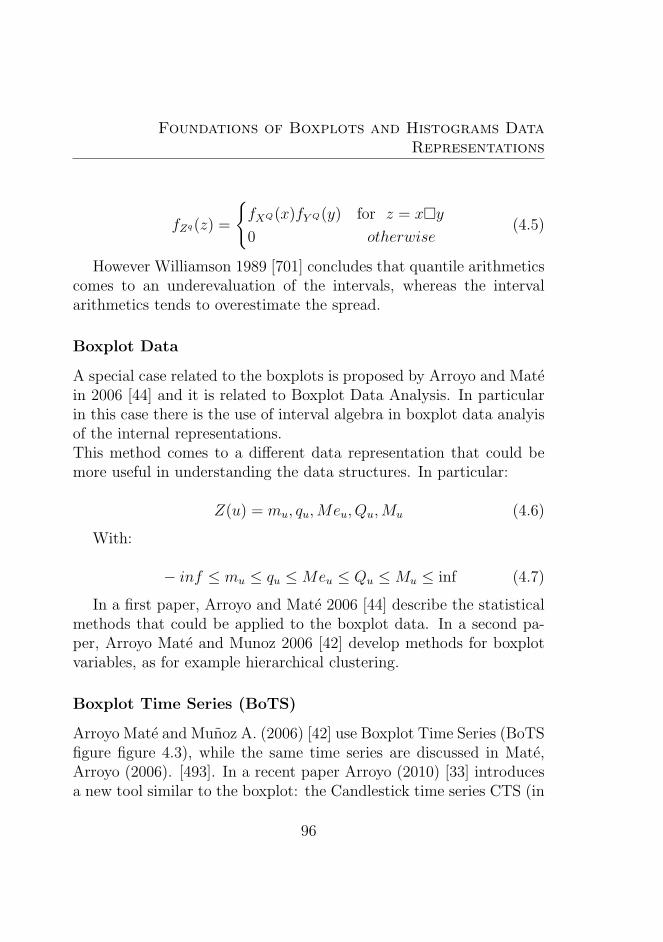
Foundations of Boxplots and Histograms DataRepresentations
fZq(z) =
fXQ(x)fY Q(y) for z = xy
0 otherwise(4.5)
However Williamson 1989 [701] concludes that quantile arithmeticscomes to an underevaluation of the intervals, whereas the intervalarithmetics tends to overestimate the spread.
Boxplot Data
A special case related to the boxplots is proposed by Arroyo and Matein 2006 [44] and it is related to Boxplot Data Analysis. In particularin this case there is the use of interval algebra in boxplot data analyisof the internal representations.This method comes to a different data representation that could bemore useful in understanding the data structures. In particular:
Z(u) = mu, qu,Meu, Qu,Mu (4.6)
With:
− inf ≤ mu ≤ qu ≤Meu ≤ Qu ≤Mu ≤ inf (4.7)
In a first paper, Arroyo and Mate 2006 [44] describe the statisticalmethods that could be applied to the boxplot data. In a second pa-per, Arroyo Mate and Munoz 2006 [42] develop methods for boxplotvariables, as for example hierarchical clustering.
Boxplot Time Series (BoTS)
Arroyo Mate and Munoz A. (2006) [42] use Boxplot Time Series (BoTSfigure figure 4.3), while the same time series are discussed in Mate,Arroyo (2006). [493]. In a recent paper Arroyo (2010) [33] introducesa new tool similar to the boxplot: the Candlestick time series CTS (in
96
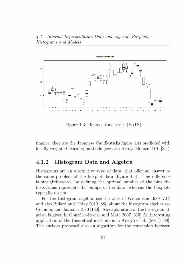
4.1. Internal Representation Data and Algebra: Boxplots,Histograms and Models
Figure 4.3: Boxplot time series (BoTS)
finance, they are the Japanese Candlesticks figure 4.4) predicted withlocally weighted learning methods (see also Arroyo Bomze 2010 [35])
4.1.2 Histogram Data and Algebra
Histograms are an alternative type of data, that offer an answer tothe same problem of the boxplot data (figure 4.5). The differenceis straightforward, by defining the optimal number of the bins thehistograms represents the bumps of the data, whereas the boxplotstypically do not.
For the Histogram algebra, see the work of Williamson 1989 [701]and also Billard and Diday 2010 [88], about the histogram algebra seeColombo and Jaarsma 1980 [150]. An explanation of the histogram al-gebra is given in Gonzales-Rıvera and Mate 2007 [315] An interestingapplication of the theoretical methods is in Arroyo et al. (2011) [38].The authors proposed also an algorithm for the conversion between
97
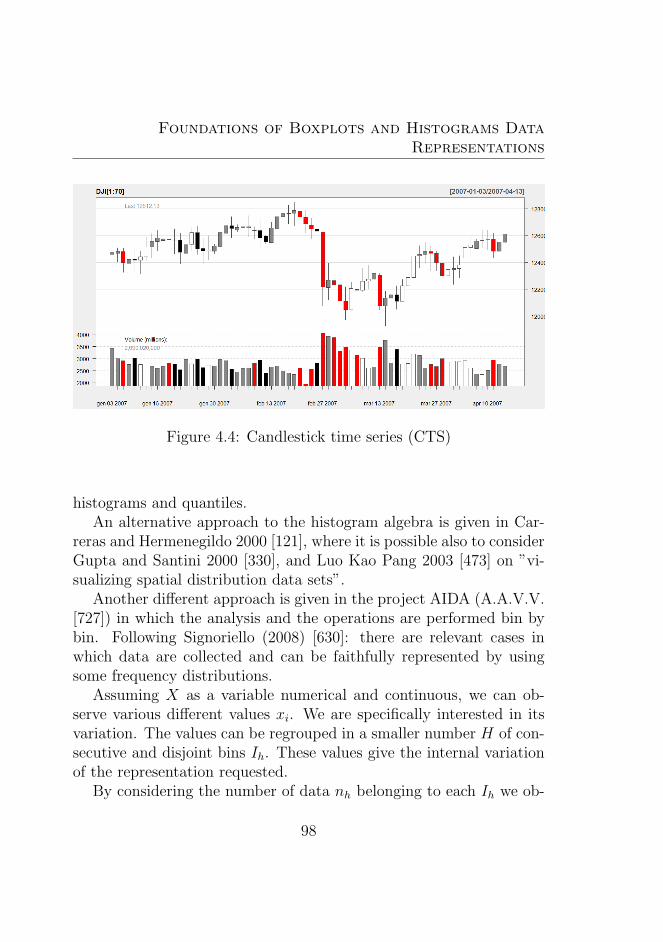
Foundations of Boxplots and Histograms DataRepresentations
Figure 4.4: Candlestick time series (CTS)
histograms and quantiles.An alternative approach to the histogram algebra is given in Car-
reras and Hermenegildo 2000 [121], where it is possible also to considerGupta and Santini 2000 [330], and Luo Kao Pang 2003 [473] on ”vi-sualizing spatial distribution data sets”.
Another different approach is given in the project AIDA (A.A.V.V.[727]) in which the analysis and the operations are performed bin bybin. Following Signoriello (2008) [630]: there are relevant cases inwhich data are collected and can be faithfully represented by usingsome frequency distributions.
Assuming X as a variable numerical and continuous, we can ob-serve various different values xi. We are specifically interested in itsvariation. The values can be regrouped in a smaller number H of con-secutive and disjoint bins Ih. These values give the internal variationof the representation requested.
By considering the number of data nh belonging to each Ih we ob-
98
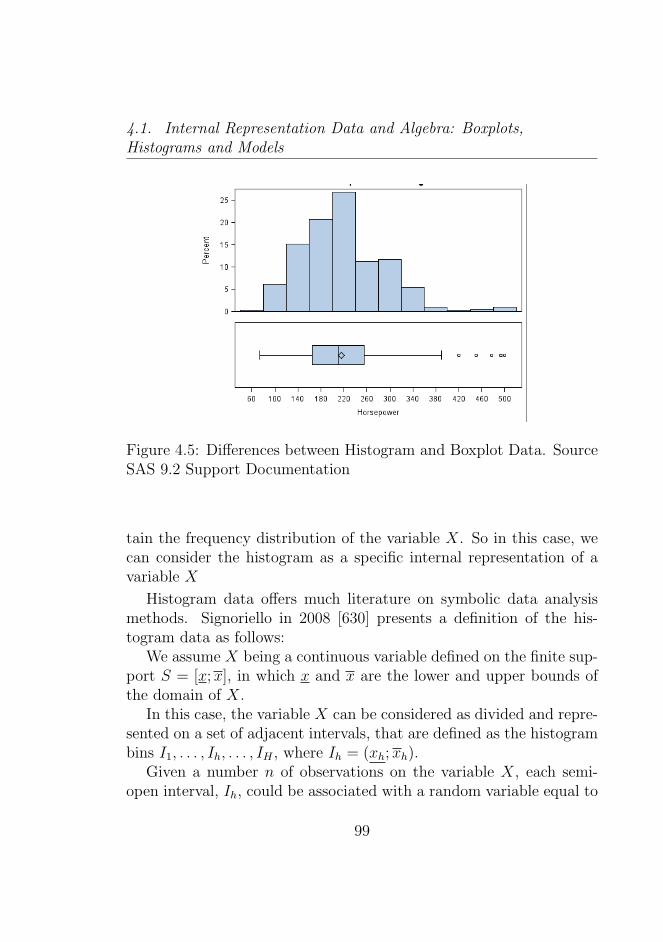
4.1. Internal Representation Data and Algebra: Boxplots,Histograms and Models
Figure 4.5: Differences between Histogram and Boxplot Data. SourceSAS 9.2 Support Documentation
tain the frequency distribution of the variable X. So in this case, wecan consider the histogram as a specific internal representation of avariable X
Histogram data offers much literature on symbolic data analysismethods. Signoriello in 2008 [630] presents a definition of the his-togram data as follows:
We assume X being a continuous variable defined on the finite sup-port S = [x;x], in which x and x are the lower and upper bounds ofthe domain of X.
In this case, the variable X can be considered as divided and repre-sented on a set of adjacent intervals, that are defined as the histogrambins I1, . . . , Ih, . . . , IH , where Ih = (xh;xh).
Given a number n of observations on the variable X, each semi-open interval, Ih, could be associated with a random variable equal to
99
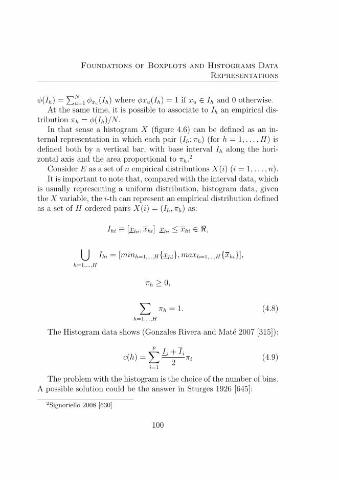
Foundations of Boxplots and Histograms DataRepresentations
φ(Ih) =∑N
u=1 φxu(Ih) where φxu(Ih) = 1 if xu ∈ Ih and 0 otherwise.At the same time, it is possible to associate to Ih an empirical dis-
tribution πh = φ(Ih)/N .In that sense a histogram X (figure 4.6) can be defined as an in-
ternal representation in which each pair (Ih; πh) (for h = 1, . . . , H) isdefined both by a vertical bar, with base interval Ih along the hori-zontal axis and the area proportional to πh.
2
Consider E as a set of n empirical distributions X(i) (i = 1, . . . , n).It is important to note that, compared with the interval data, which
is usually representing a uniform distribution, histogram data, giventhe X variable, the i-th can represent an empirical distribution definedas a set of H ordered pairs X(i) = (Ih, πh) as:
Ihi ≡ [xhi, xhi] xhi ≤ xhi ∈ <,
⋃h=1,...,H
Ihi = [minh=1,...,Hxhi,maxh=1,...,Hxhi],
πh ≥ 0,
∑h=1,...,H
πh = 1. (4.8)
The Histogram data shows (Gonzales Rivera and Mate 2007 [315]):
c(h) =
p∑i=1
I i + I i2
πi (4.9)
The problem with the histogram is the choice of the number of bins.A possible solution could be the answer in Sturges 1926 [645]:
2Signoriello 2008 [630]
100
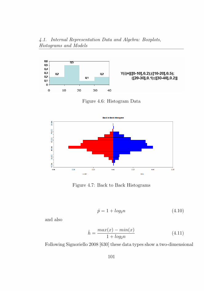
4.1. Internal Representation Data and Algebra: Boxplots,Histograms and Models
Figure 4.6: Histogram Data
Figure 4.7: Back to Back Histograms
p = 1 + log2n (4.10)
and also
h =max(x)−min(x)
1 + log2n(4.11)
Following Signoriello 2008 [630] these data types show a two-dimensional
101
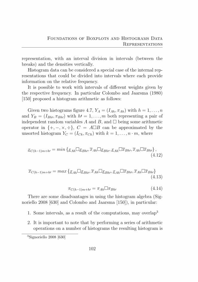
Foundations of Boxplots and Histograms DataRepresentations
representation, with an interval division in intervals (between thebreaks) and the densities vertically.
Histogram data can be considered a special case of the internal rep-resentations that could be divided into intervals where each provideinformation on the relative frequency.
It is possible to work with intervals of different weights given bythe respective frequency. In particular Colombo and Jaarsma (1980)[150] proposed a histogram arithmetic as follows:
Given two histograms figure 4.7, YA = (IAh, πAh) with h = 1, . . . , nand YB = (IBh′, πBh′) with h′ = 1, . . . ,m both representing a pair ofindependent random variables A and B, and being some arithmeticoperator in +,−,×,÷, C = AB can be approximated by theunsorted histogram YC = (ICk, πCk) with k = 1, . . . , n ·m, where
xC(h−1)m+h′ = min xAhxBh′, xAhxBh′, xAhxBh′, xAhxBh′ ,(4.12)
xC(h−1)m+h′ = max xAhxBh′, xAhxBh′, xAhxBh′, xAhxBh′(4.13)
πC(h−1)m+h′ = πAhπBh′ (4.14)
There are some disadvantages in using the histogram algebra (Sig-noriello 2008 [630] and Colombo and Jaarsma [150]), in particular:
1. Some intervals, as a result of the computations, may overlap3
2. It is important to note that by performing a series of arithmeticoperations on a number of histograms the resulting histogram is
3Signoriello 2008 [630]
102
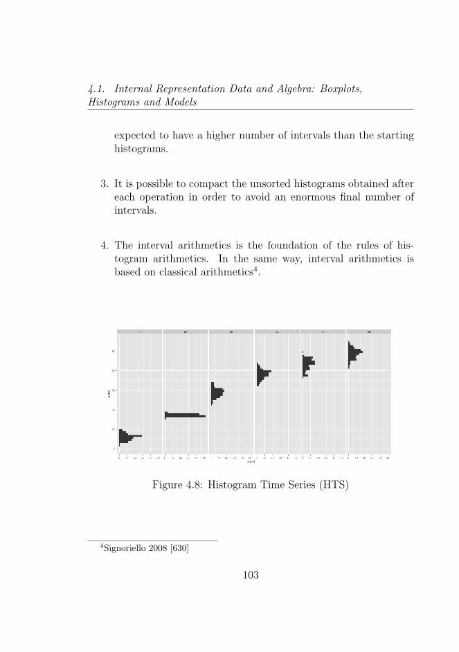
4.1. Internal Representation Data and Algebra: Boxplots,Histograms and Models
expected to have a higher number of intervals than the startinghistograms.
3. It is possible to compact the unsorted histograms obtained aftereach operation in order to avoid an enormous final number ofintervals.
4. The interval arithmetics is the foundation of the rules of his-togram arithmetics. In the same way, interval arithmetics isbased on classical arithmetics4.
Figure 4.8: Histogram Time Series (HTS)
4Signoriello 2008 [630]
103
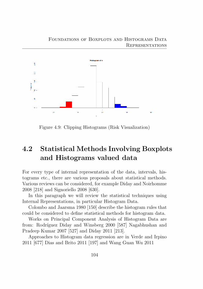
Foundations of Boxplots and Histograms DataRepresentations
Figure 4.9: Clipping Histograms (Risk Visualization)
4.2 Statistical Methods Involving Boxplots
and Histograms valued data
For every type of internal representation of the data, intervals, his-tograms etc., there are various proposals about statistical methods.Various reviews can be considered, for example Diday and Noirhomme2008 [218] and Signoriello 2008 [630].
In this paragraph we will review the statistical techniques usingInternal Representations, in particular Histogram Data.
Colombo and Jaarsma 1980 [150] describe the histogram rules thatcould be considered to define statistical methods for histogram data.
Works on Principal Component Analysis of Histogram Data arefrom: Rodrıguez Diday and Winsberg 2000 [587] Nagabhushan andPradeep Kumar 2007 [527] and Diday 2011 [213].
Approaches to Histogram data regression are in Verde and Irpino2011 [677] Dias and Brito 2011 [197] and Wang Guan Wu 2011
104
4.3. Internal Representations Models
.
4.2.1 Histogram Stochastic Processes and HistogramTime Series (HTS)
Very recent and relevant is the growth in literature of the symbolicforecasting methods using histogram time series (HTS figure 4.8). Ar-royo and Mate 2009 analyse in depth interval data forecasting methodsusing KNN K-Neirest Neighbour methods [44]. Gonzales Rivera andArroyo 2011 [319] and [318] define the concept of the histogram ran-dom variable and stochastic process. The stochastic process can bedefined as: A histogram-valued stochastic process is a collection ofhistogram random variables that are indexed by time. A histogramtime series (HTS) is the realization of a histogram valued stochas-tic process. A histogram valued stochastic process can be definedas weak stationary if every interval are weakly stationary processes.An important definition is the barycentric histogram that minimizesthe distances with other histograms and is obtained by optimization.The authors derive the empirical autocorrelation with respect to thebarycenter (See Gonzales Rivera and Arroyo 2011 [319] and [318]). Animportant way to analyse histogram time series (HTS) is to considerquantile intervals in the histograms (figure 4.9), in particular Gonza-les Rivera and Arroyo 2011 [318] show the usefulness of this type ofanalysis.
4.3 Internal Representations Models
Until now, we have assumed that initial data are not affected by theexisting error. There are important cases in which this assumption isuntenable. In these cases, it is necessary to consider the existence ofthe noise in the data, and ”model” the data accordingly. According to
105
Foundations of Boxplots and Histograms DataRepresentations
Signoriello (2008) [630], and also Drago, Lauro and Scepi 2009 [233],sometimes it can be very useful to model the shape of the initial data(say, a histogram or later the density data) to extract the relevantinformation from our data. In this case, we are taking into accountthe errors present in data in a wide sense (for example missing value,or other phenomena)5. We define data model as specific data, in whichwe have eliminated the measurement error.
It is important to note real models do not exist but any model canbe an approximation of the reality. A model is good if it is useful asapproximation. In this sense, only models that could be validated bydata can be useful.Tukey in a work of 1977 [670] and Caussinus in 1986 [123] allow inwhat sense it is possible to interpret the statistical methods (bothconfirmatory and exploratory) by approximating initial data as:
Data = Structural Part+Noise (4.15)
Where D are the data, S is the structural part and N is the noise.This idea is relevant for example in the time series analysis, in whichwe want to extract the signal from the noise.
The idea proposed by Signoriello 2008 [630] and Drago, Lauro andScepi 2009 [233] is that of specifically transforming the histogram databy using an approximation function to control the error (or the noiseE) deriving from empirical data figure 4.10.In this case, if we assume the structural part as our model we canreformulate the empirical data as:
Data = Model + Error (4.16)
Here M is the model used and E the error. In this case the data arespecifically obtained by the approximated function in the modelling
5Signoriello 2008 [630]
106
4.4. The Data Choice
process and we obtain the model coefficients and an index of goodnessof fit.The general problem is to find some functions (the models) that opti-mally approximate the initial data (histogram, for example) as poly-nomial models, splines, or B-splines. Each different model can becharacterised by a goodness of fit (an evaluation index of the qualityof the representation of the initial data). Later we will express thesedata as a finite mixture model in which we obtain the same result toextract the relevant information from the original data.
So for each i-observation we obtain a specific n-function. It is pos-sible to represent the coefficients as in the figure. It is important tonote that the original histograms or the original data are substitutedby their coefficients.
4.4 The Data Choice
Simple examples of conversion between different data types are inArroyo et al. 2011 [38] in which the authors propose an algorithm totransform initial histogram data into quantiles.
4.4.1 The Optimal Data Choice
The choice of the best interval representation data is attributed tothe analyst and to the specific analysis (so they can be considereda choice to perform a priori). Where there is not a specific a prioripreferred data type there are two fundamental factors that need to beconsidered:
1. A genuine data type (in the sense there is no possibility of choicebecause the data needs to be considered).
107
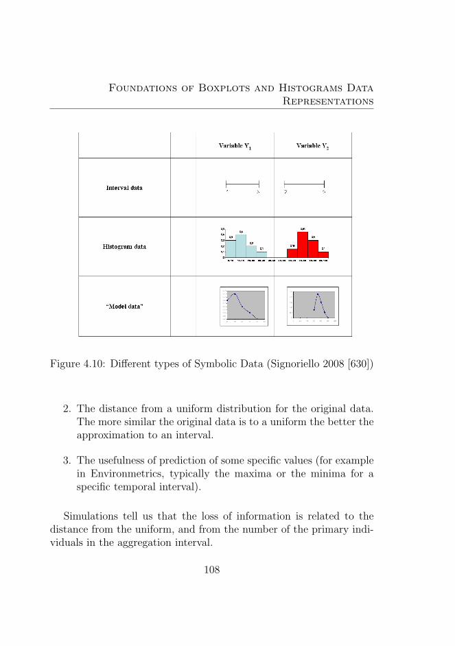
Foundations of Boxplots and Histograms DataRepresentations
Figure 4.10: Different types of Symbolic Data (Signoriello 2008 [630])
2. The distance from a uniform distribution for the original data.The more similar the original data is to a uniform the better theapproximation to an interval.
3. The usefulness of prediction of some specific values (for examplein Environmetrics, typically the maxima or the minima for aspecific temporal interval).
Simulations tell us that the loss of information is related to thedistance from the uniform, and from the number of the primary indi-viduals in the aggregation interval.
108
4.4. The Data Choice
4.4.2 Conversions between Data
It is possible to convert the data, when the internal representationbecome from a summary of huge sets of data, see Diday Esposito2003 [216]. In fact, from the database queries we can extract differentcategories of descriptive variables. At the same time, a specific repre-sentation comes from the use of a multidimensional specific techniquethat perform a partitioning in the original massive data set. In allthese cases, it is possible to change the internal representation of thedata; where the data is specifically native this practice is straightfor-ward, see for example Diday and Noirhomme 2008 [218]. There is aunique problem to consider in the choice, that one choice or anotherone could determine a specific loss of the variability of the data [212].The problem is clear when it is necessary to transform the originalinternal representation into classical data here there is a loss of in-formation (due to the fact that the classical data does not considervariation).
So when the data shares a strong internal variability and hetero-geneity, they need to be represented as internal representations overtime or over space by taking into account this variability.
109

Foundations of Boxplots and Histograms DataRepresentations
Summary Results: HistogramsAn Internal Representation preserving complex patterns of intra-data variation.Histogram Algebra can be built on Interval Algebra.It is possible to estimate the relevant coefficients to obtain the DataModels (Histograms can be parameterized to obtain Data Models).
110
Chapter 5
Foundations of DensityValued Data:Representations
In general, it is possible to use other statistical methods to representsome data. In this way, the histogram or the boxplot (both seen inChapter 4) are a type of the representation that could be possible tobe considered. In literature it is sometimes suggested to use kerneldensity estimators instead of histograms for the smoothness and thebin placement (see a discussion in Di Nardo Tobias 2001 [222] but alsoin Gelman 2009 [293] for a discussion of the topic), in fact both arenonparametric methods which do not impose any type of specific para-metric form. In the histogram case1, in practice, bins can determinethe shape of the density and the discontinuities and sometimes it isuseful to explore also this aspect by removing the discontinuity2. So,
1There are at the same time proposals for different histogram types, see forexample: [195]
2The histograms by definition are not smooth. The histogram shape dependson the bin width and the end point of the same bins. In this way in constructing
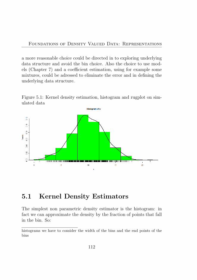
Foundations of Density Valued Data: Representations
a more reasonable choice could be directed in to exploring underlyingdata structure and avoid the bin choice. Also the choice to use mod-els (Chapter 7) and a coefficient estimation, using for example somemixtures, could be adressed to eliminate the error and in defining theunderlying data structure.
Figure 5.1: Kernel density estimation, histogram and rugplot on sim-ulated data
5.1 Kernel Density Estimators
The simplest non parametric density estimator is the histogram: infact we can approximate the density by the fraction of points that fallin the bin. So:
histograms we have to consider the width of the bins and the end points of thebins
112
5.1. Kernel Density Estimators
f(x) =1
nh
n∑i=1
1xi (5.1)
Where xi is in the same bin as x (Racine 2008 [569]) and 1(A) isan indicator function with value 1 if A is true, zero otherwise.
In this sense the histogram construction3, can start from an originx0 and a bin width h. The bins can be considered as [x0 + mh, x0 +(m+ 1)h] both for positive and negative integers4.
It is possible to represent a histogram by smoothing their bins (fig-ure 5.1 and figure 5.3 and obtaining a single continued function f(x).So the kernel density estimator is5:
f(x) =1
nh
n∑i=1
K(x− xih
) (5.2)
where K(z) is a Kernel, a symmetric weight function and h is asmoothing parameter defined as a bandwidth6. The bandwidth choicein this case is very important7. In fact from the h depends the level ofsmoothness of the density. For the bandwidth selection problem seeTurlach 1993 [669], Chiu 1991 [139], Hart Vieu 1990 [342]. In general apresentation and a review of a nonparametric approach is to be foundin Li and Racine 2005 [465].K can be a gaussian function with mean zero and variance 1. The
Kernel is a non-negative and real-valued function K(z) satisfying:
3In particular (Milani 2008 [504]) for a review of the graphical exploratorytechniques
4Li Racine 2007 [465] and also Racine 2008 [569]5Racine 2008 [569] and Pagan Ullah (1999) [542]6Racine 2008 [569] states that this estimator could be defined as the Rosenblatt–
Parzen estimator: see Rosenblatt (1956) [595] and Parzen (1962) [549]. Where thexi are time series or dependent data: see Hansen 2009 [338] Wand and Jones 2005[687] and Harvey and Oryshchenko 2010 [345]
7Katkovnik Shimulevich 2000 [419] Silverman 1978 [633] and Raudys 1991 [578]
113
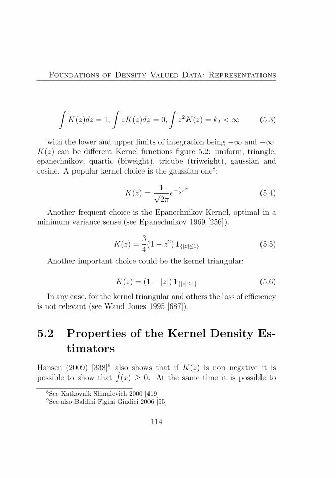
Foundations of Density Valued Data: Representations
∫K(z)dz = 1,
∫zK(z)dz = 0,
∫z2K(z) = k2 <∞ (5.3)
with the lower and upper limits of integration being −∞ and +∞.K(z) can be different Kernel functions figure 5.2: uniform, triangle,epanechnikov, quartic (biweight), tricube (triweight), gaussian andcosine. A popular kernel choice is the gaussian one8:
K(z) =1√2πe−
12z2
(5.4)
Another frequent choice is the Epanechnikov Kernel, optimal in aminimum variance sense (see Epanechnikov 1969 [256]).
K(z) =3
4(1− z2) 1|z|≤1 (5.5)
Another important choice could be the kernel triangular:
K(z) = (1− |z|) 1|z|≤1 (5.6)
In any case, for the kernel triangular and others the loss of efficiencyis not relevant (see Wand Jones 1995 [687]).
5.2 Properties of the Kernel Density Es-
timators
Hansen (2009) [338]9 also shows that if K(z) is non negative it ispossible to show that f(x) ≥ 0. At the same time it is possible to
8See Katkovnik Shmulevich 2000 [419]9See also Baldini Figini Giudici 2006 [55]
114
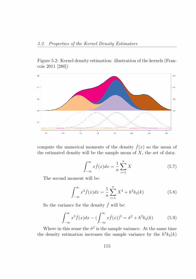
5.2. Properties of the Kernel Density Estimators
Figure 5.2: Kernel density estimation: illustration of the kernels (Fran-cois 2011 [280])
compute the numerical moments of the density f(x) so the mean ofthe estimated density will be the sample mean of X, the set of data:∫ ∞
−∞xf(x)dx =
1
n
n∑i=1
X (5.7)
The second moment will be:∫ ∞−∞
x2f(x)dx =1
n
n∑i=1
X2 + h2k2(k) (5.8)
So the variance for the density f will be:∫ ∞−∞
x2f(x)dx− (
∫ ∞−∞
xf(x))2 = σ2 + h2k2(k) (5.9)
Where in this sense the σ2 is the sample variance. At the same timethe density estimation increases the sample variance by the h2k2(k)
115
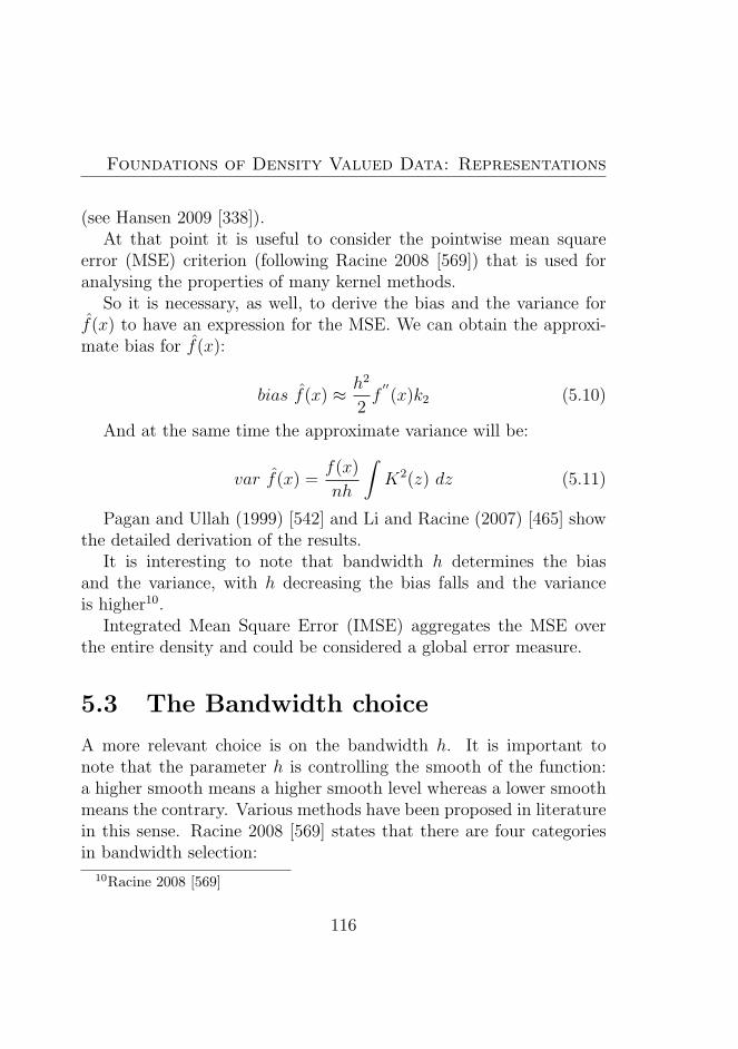
Foundations of Density Valued Data: Representations
(see Hansen 2009 [338]).At that point it is useful to consider the pointwise mean square
error (MSE) criterion (following Racine 2008 [569]) that is used foranalysing the properties of many kernel methods.
So it is necessary, as well, to derive the bias and the variance forf(x) to have an expression for the MSE. We can obtain the approxi-mate bias for f(x):
bias f(x) ≈ h2
2f′′(x)k2 (5.10)
And at the same time the approximate variance will be:
var f(x) =f(x)
nh
∫K2(z) dz (5.11)
Pagan and Ullah (1999) [542] and Li and Racine (2007) [465] showthe detailed derivation of the results.
It is interesting to note that bandwidth h determines the biasand the variance, with h decreasing the bias falls and the varianceis higher10.
Integrated Mean Square Error (IMSE) aggregates the MSE overthe entire density and could be considered a global error measure.
5.3 The Bandwidth choice
A more relevant choice is on the bandwidth h. It is important tonote that the parameter h is controlling the smooth of the function:a higher smooth means a higher smooth level whereas a lower smoothmeans the contrary. Various methods have been proposed in literaturein this sense. Racine 2008 [569] states that there are four categoriesin bandwidth selection:
10Racine 2008 [569]
116
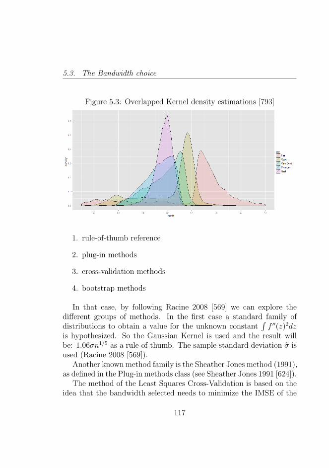
5.3. The Bandwidth choice
Figure 5.3: Overlapped Kernel density estimations [793]
1. rule-of-thumb reference
2. plug-in methods
3. cross-validation methods
4. bootstrap methods
In that case, by following Racine 2008 [569] we can explore thedifferent groups of methods. In the first case a standard family ofdistributions to obtain a value for the unknown constant
∫f ′′(z)2dz
is hypothesized. So the Gaussian Kernel is used and the result willbe: 1.06σn1/5 as a rule-of-thumb. The sample standard deviation σ isused (Racine 2008 [569]).
Another known method family is the Sheather Jones method (1991),as defined in the Plug-in methods class (see Sheather Jones 1991 [624]).
The method of the Least Squares Cross-Validation is based on theidea that the bandwidth selected needs to minimize the IMSE of the
117
Foundations of Density Valued Data: Representations
estimate.In the methods of Likelihood Cross-Validation it is necessary to
choose h to maximize the log likelihood.Faraway and Jhun (1990) [262] have proposed a different approach
based on bootstrap, in which the selection of the h is in estimatingthe IMSE and minimizing them over all bandwidths.
In addition, we consider data-driven methods, that are not a guar-antee of good results everytime11.
In the data visualization part (Chapter 6) we will use the Sheather-Jones criteria that defines the optimal h in a data-driven choice (seeKampstra 2008 [416]).
5.4 Density Algebra using Functional Data
Analysis
By using Functional Data Analysis it is possible to transform the den-sity into a functional data. The density could be considered a func-tion and so in that sense specifically used for some operations. So itis possible to consider the beanplots and transform the densities intofunctional data12
An important result in this topic is provided by Zhang 2007 [717]Zhang and Muller 2010 [720] and by Kneip Utikal 2001 [426] and Jones1992 [412]. Ramsay and Silverman [574] perform a principal compo-nents analysis of the log densities.
11Racine 2008 for an explanation. [569]12See for example Delaigle and Hall [188] who consider the approach of densities
as functional data. Another approach in this sense is provided by Delicado (2010)[189] in the approach of dimensionality reduction of densities as functional data.
118
5.5. Density Algebra using Histogram Algebra
5.5 Density Algebra using Histogram Al-
gebra
Density Algebra is a way to obtain for example the density meanbetween a group of densities by using the histogram algebra. In thissense we transform the original density data into Histograms, withregards to the method for the construction of the optimal histogramsee: Scott 1979 [617], Sheather Jones (1991) [624] and Wand (1995)[686]. The number of bins needs to be chosen for the histograms to usein the analysis. So if the histograms have the same number of bins theycan be computed, if not it is necessary to compute an average. Afterthe operation of transformations we can consider the related algebricaloperations between histogram data (see Colombo and Jaarsma 1980[150]). An explanation in terms of histogram data is given by GonzalesRivera and Mate 2007 [315]
5.6 Density Trace and Data Heterogene-
ity
Sometimes a relevant assumption on data is that they represent somepatterns of heterogeneity. Mixtures are useful to understand interest-ing patterns in data that could be detected and exploited over time t.In particular (see Ingrassia Greselin Morlini 2008 [392]) we assume aset of data Ξ that could be constituted by g different subgroups at aspecific time t, so we have Ξ = Ξ1∪ ....∪Ξg every time t. The elementsfor each t are mixed proportionally α1, ...αg. They can be, for example,prices of houses in a set of data Ξ in different zones. In that case thereis a homogeneous quantity X intra groups and a heterogeneous onebetween. The random variable X can have a probability distributiondifferent for each group, and we assume that the distribution of prob-
119
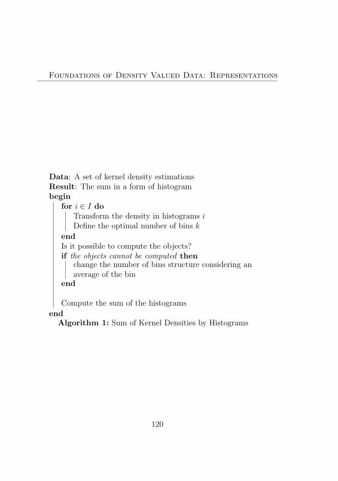
Foundations of Density Valued Data: Representations
Data: A set of kernel density estimationsResult: The sum in a form of histogrambegin
for i ∈ I doTransform the density in histograms iDefine the optimal number of bins k
endIs it possible to compute the objects?if the objects cannot be computed then
change the number of bins structure considering anaverage of the bin
end
Compute the sum of the histograms
endAlgorithm 1: Sum of Kernel Densities by Histograms
120
5.7. Conversions between Density Data and other types of data
ability intra–group are among the same parametric family f(x,Θ), inwhich the parameter θ ∈ Θ is different between the groups.
Groups can be indicized by a discrete variable S to values into1, ..., g. The probability to choose the group S = j with j ∈ (1...g) isindicated with l(j) and is equal to αj(j = 1...g). The joint probabilitydensity p(x, j) is:
p(x, j) = p(x|j)l(j) = f(x|θj)l(j) (5.12)
Where in each mixture model we observe only the random variableX. The marginal density of X is:
p(x; Ψ) =
g∑j=1
p(x, j) = α1f(x|θ1) + ...αgf(x|θg) (5.13)
Where in Ψ is a vector with all the parameters of the model. In thatsense in a specific temporal interval t we can have elements belongingto different groups g, for example due to some effects. So for each timet we can consider different mixture models. These types of models canbe important in financial data where mixture models seem to be veryuseful for returns.
5.7 Conversions between Density Data and
other types of data
At the same time, it is possible to transform the density data intoother types of data or representations like histograms (Algorithm 1.)or intervals etc. In particular following Wand Jones 1995 [687] andSheather and Jones 1991 [624], we can obtain the binned approxima-tion to the kernel estimate of the density functional [687]. So we cantranslate a specific beanplot or density data into a specific histogram.
121
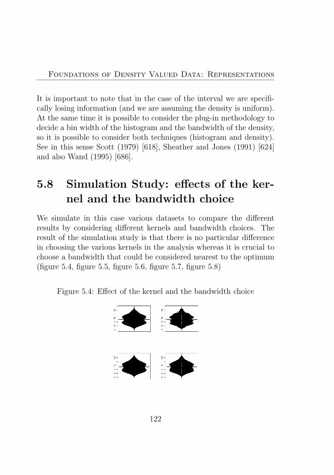
Foundations of Density Valued Data: Representations
It is important to note that in the case of the interval we are specifi-cally losing information (and we are assuming the density is uniform).At the same time it is possible to consider the plug-in methodology todecide a bin width of the histogram and the bandwidth of the density,so it is possible to consider both techniques (histogram and density).See in this sense Scott (1979) [618], Sheather and Jones (1991) [624]and also Wand (1995) [686].
5.8 Simulation Study: effects of the ker-
nel and the bandwidth choice
We simulate in this case various datasets to compare the differentresults by considering different kernels and bandwidth choices. Theresult of the simulation study is that there is no particular differencein choosing the various kernels in the analysis whereas it is crucial tochoose a bandwidth that could be considered nearest to the optimum(figure 5.4, figure 5.5, figure 5.6, figure 5.7, figure 5.8)
Figure 5.4: Effect of the kernel and the bandwidth choice
122
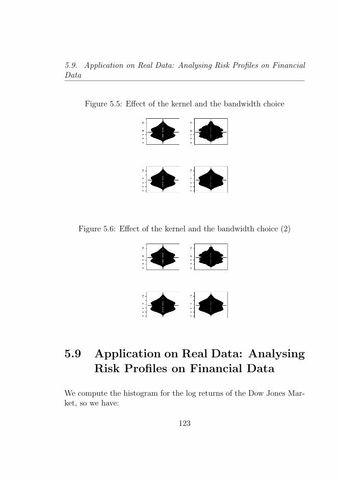
5.9. Application on Real Data: Analysing Risk Profiles on FinancialData
Figure 5.5: Effect of the kernel and the bandwidth choice
Figure 5.6: Effect of the kernel and the bandwidth choice (2)
5.9 Application on Real Data: Analysing
Risk Profiles on Financial Data
We compute the histogram for the log returns of the Dow Jones Mar-ket, so we have:
123
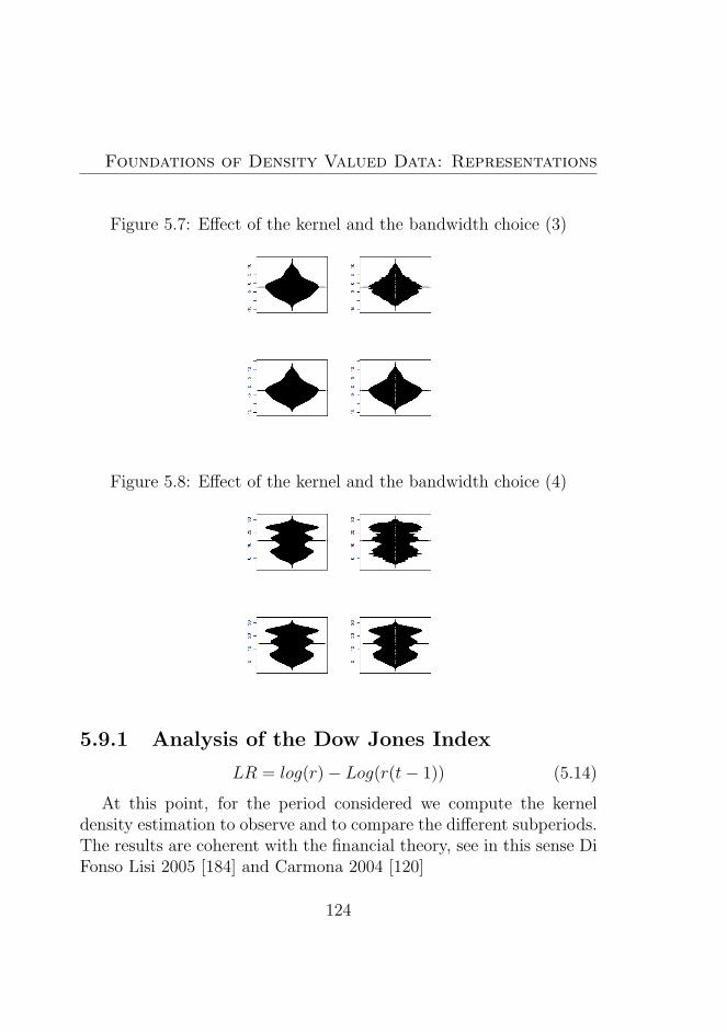
Foundations of Density Valued Data: Representations
Figure 5.7: Effect of the kernel and the bandwidth choice (3)
Figure 5.8: Effect of the kernel and the bandwidth choice (4)
5.9.1 Analysis of the Dow Jones Index
LR = log(r)− Log(r(t− 1)) (5.14)
At this point, for the period considered we compute the kerneldensity estimation to observe and to compare the different subperiods.The results are coherent with the financial theory, see in this sense DiFonso Lisi 2005 [184] and Carmona 2004 [120]
124
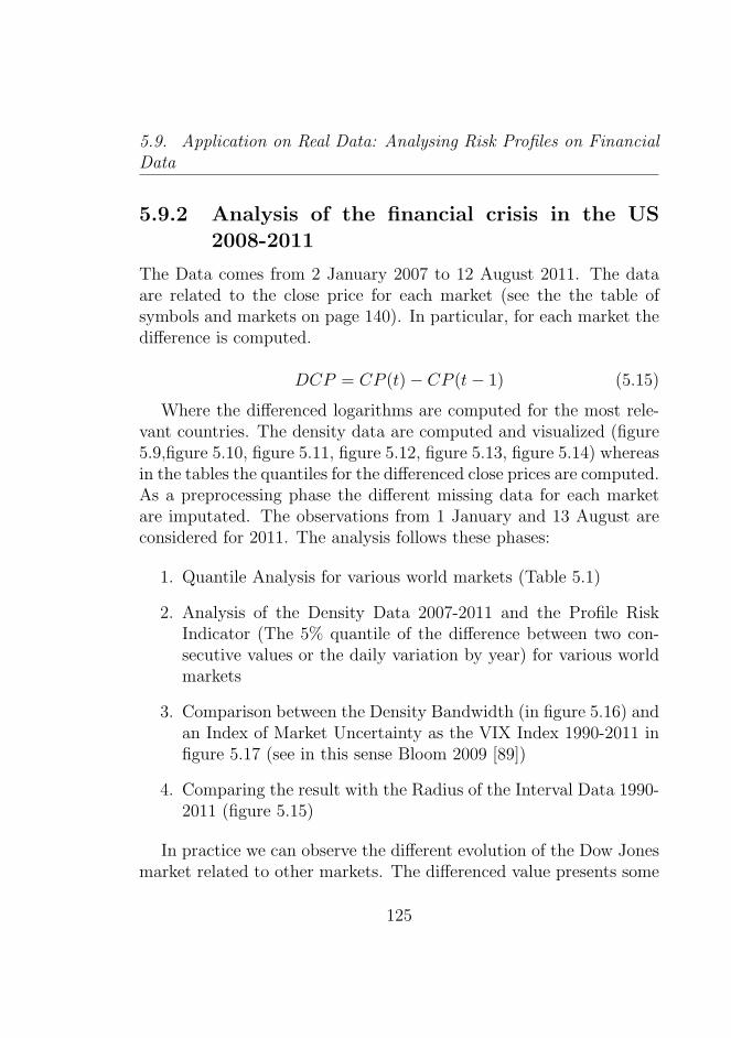
5.9. Application on Real Data: Analysing Risk Profiles on FinancialData
5.9.2 Analysis of the financial crisis in the US2008-2011
The Data comes from 2 January 2007 to 12 August 2011. The dataare related to the close price for each market (see the the table ofsymbols and markets on page 140). In particular, for each market thedifference is computed.
DCP = CP (t)− CP (t− 1) (5.15)
Where the differenced logarithms are computed for the most rele-vant countries. The density data are computed and visualized (figure5.9,figure 5.10, figure 5.11, figure 5.12, figure 5.13, figure 5.14) whereasin the tables the quantiles for the differenced close prices are computed.As a preprocessing phase the different missing data for each marketare imputated. The observations from 1 January and 13 August areconsidered for 2011. The analysis follows these phases:
1. Quantile Analysis for various world markets (Table 5.1)
2. Analysis of the Density Data 2007-2011 and the Profile RiskIndicator (The 5% quantile of the difference between two con-secutive values or the daily variation by year) for various worldmarkets
3. Comparison between the Density Bandwidth (in figure 5.16) andan Index of Market Uncertainty as the VIX Index 1990-2011 infigure 5.17 (see in this sense Bloom 2009 [89])
4. Comparing the result with the Radius of the Interval Data 1990-2011 (figure 5.15)
In practice we can observe the different evolution of the Dow Jonesmarket related to other markets. The differenced value presents some
125

Foundations of Density Valued Data: Representations
interesting features related to the volatility that could be effectivelycaptured by the density data. For each year we can note that thereare some economic situations (US, Italy, France, Germany, Brazil forexample) that in different situations are behaving differently and canhave different market responses to the shocks (see Bloom 2009 [89]).In particular it seems possible to observe, considering the bandwidthsequence extracted year by year from the US data, that they are ca-pable of identifying well the most relevant financial shocks on themarket (see in this sense [90]). It is at the same time confirmed thatthe methods considered here allow one to observe phenomena like theimplied volatility over the time and perhaps anticipate them by usingsome forecasting methods over time. The use of density permits oneto observe the entire data structure, as will be seen in the followingchapters.
126
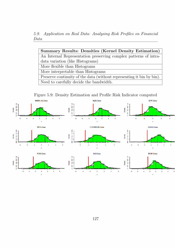
5.9. Application on Real Data: Analysing Risk Profiles on FinancialData
Summary Results: Densities (Kernel Density Estimation)An Internal Representation preserving complex patterns of intra-data variation (like Histograms)More flexible than HistogramsMore interpretable than HistogramsPreserve continuity of the data (without representing it bin by bin).Need to carefully decide the bandwidth.
Figure 5.9: Density Estimation and Profile Risk Indicator computed
127
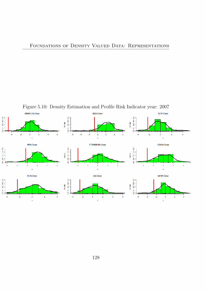
Foundations of Density Valued Data: Representations
Figure 5.10: Density Estimation and Profile Risk Indicator year: 2007
128
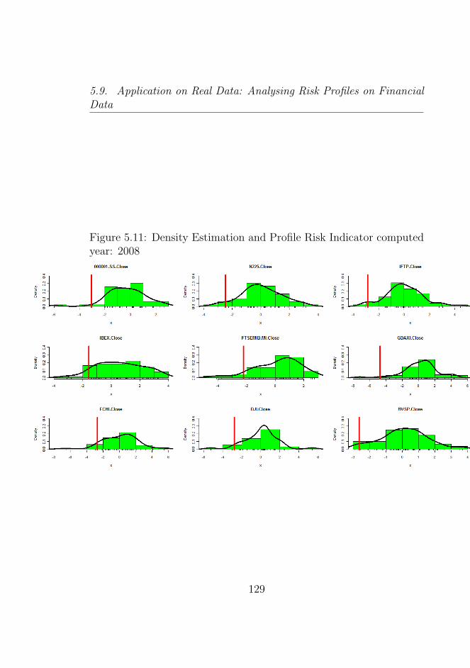
5.9. Application on Real Data: Analysing Risk Profiles on FinancialData
Figure 5.11: Density Estimation and Profile Risk Indicator computedyear: 2008
129
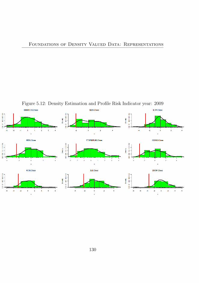
Foundations of Density Valued Data: Representations
Figure 5.12: Density Estimation and Profile Risk Indicator year: 2009
130
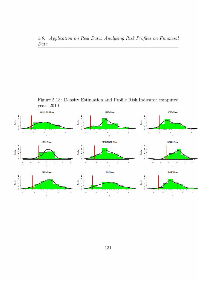
5.9. Application on Real Data: Analysing Risk Profiles on FinancialData
Figure 5.13: Density Estimation and Profile Risk Indicator computedyear: 2010
131
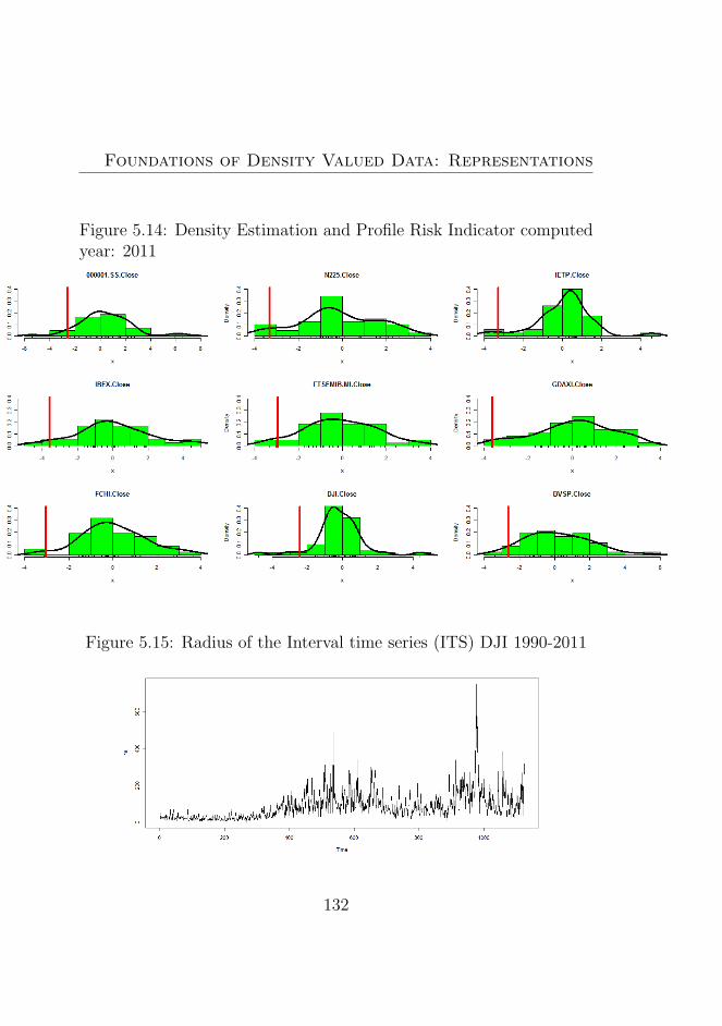
Foundations of Density Valued Data: Representations
Figure 5.14: Density Estimation and Profile Risk Indicator computedyear: 2011
Figure 5.15: Radius of the Interval time series (ITS) DJI 1990-2011
132
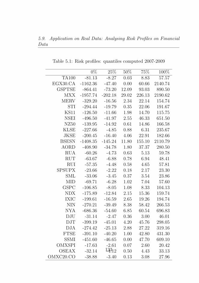
5.9. Application on Real Data: Analysing Risk Profiles on FinancialData
Table 5.1: Risk profiles: quantiles computed 2007-2009
0% 25% 50% 75% 100%TA100 -81.13 -8.27 0.03 8.83 57.57
EGX30.CA -1162.36 -47.40 0.00 60.66 2140.74GSPTSE -864.41 -73.20 12.09 93.03 890.50
MXX -1957.74 -202.18 29.02 226.13 2190.62MERV -329.20 -16.56 2.34 22.14 154.74
STI -294.44 -19.79 0.35 22.06 191.67KS11 -126.50 -11.66 1.98 14.70 115.75NSEI -496.50 -41.97 2.55 46.33 651.50NZ50 -139.95 -14.92 0.61 14.86 166.58KLSE -227.66 -4.85 0.88 6.31 235.67JKSE -200.45 -16.40 4.06 22.91 182.66
BSESN -1408.35 -145.24 11.80 155.10 2110.79AORD -408.90 -34.78 1.80 37.37 280.50
RUA -60.26 -4.73 0.63 5.13 59.78RUT -63.67 -6.88 0.78 6.94 48.41RUI -57.35 -4.48 0.58 4.65 57.81
SPSUPX -23.66 -2.22 0.18 2.17 23.30SML -33.06 -3.45 0.37 3.54 23.86MID -69.71 -6.28 1.02 7.04 57.60
GSPC -106.85 -8.05 1.08 8.33 104.13NDX -175.89 -12.84 2.15 15.36 159.74IXIC -199.61 -16.59 2.65 19.26 194.74NIN -270.21 -39.49 8.38 58.42 266.53
NYA -686.36 -54.60 6.85 60.54 696.83DJU -31.14 -2.47 0.36 3.00 46.01DJT -399.19 -45.01 4.20 45.76 298.05DJA -274.42 -25.13 2.88 27.22 319.16
FTSE -391.10 -40.20 1.00 42.80 431.30SSMI -451.60 -46.65 0.00 47.70 609.10
OMXSPI -17.63 -2.61 0.07 2.60 20.42OSEAX -32.14 -4.12 0.50 4.43 33.13
OMXC20.CO -38.88 -3.40 0.13 3.08 27.96
133
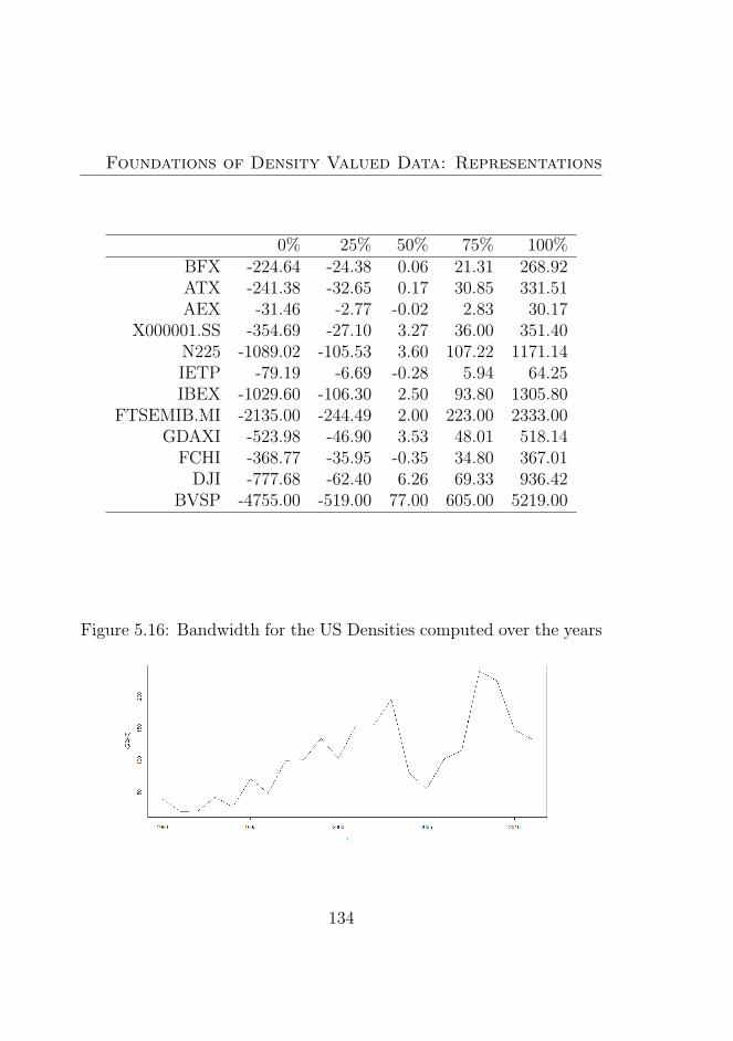
Foundations of Density Valued Data: Representations
0% 25% 50% 75% 100%BFX -224.64 -24.38 0.06 21.31 268.92ATX -241.38 -32.65 0.17 30.85 331.51AEX -31.46 -2.77 -0.02 2.83 30.17
X000001.SS -354.69 -27.10 3.27 36.00 351.40N225 -1089.02 -105.53 3.60 107.22 1171.14IETP -79.19 -6.69 -0.28 5.94 64.25IBEX -1029.60 -106.30 2.50 93.80 1305.80
FTSEMIB.MI -2135.00 -244.49 2.00 223.00 2333.00GDAXI -523.98 -46.90 3.53 48.01 518.14
FCHI -368.77 -35.95 -0.35 34.80 367.01DJI -777.68 -62.40 6.26 69.33 936.42
BVSP -4755.00 -519.00 77.00 605.00 5219.00
Figure 5.16: Bandwidth for the US Densities computed over the years
134

5.9. Application on Real Data: Analysing Risk Profiles on FinancialData
Table 5.2: International Stockmarket Symbols
Symbol Country1 TA100 Israel2 EGX30.CA Egypt3 GSPTSE Canada4 MXX Mexico5 MERV Argentina6 STI Singapore7 KS11 South Korea8 NSEI India9 NZ50 New Zealand
10 KLSE Malaysia11 JKSE Thailand12 BSESN India13 AORD Australia14 RUA USA15 RUT USA16 RUI USA17 SPSUPX USA18 SML USA19 MID USA20 GSPC USA21 NDX USA22 IXIC USA23 NIN USA24 NYA USA25 DJU USA26 DJT USA27 DJA USA
135
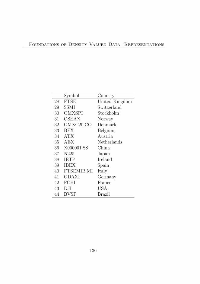
Foundations of Density Valued Data: Representations
Symbol Country28 FTSE United Kingdom29 SSMI Switzerland30 OMXSPI Stockholm31 OSEAX Norway32 OMXC20.CO Denmark33 BFX Belgium34 ATX Austria35 AEX Netherlands36 X000001.SS China37 N225 Japan38 IETP Ireland39 IBEX Spain40 FTSEMIB.MI Italy41 GDAXI Germany42 FCHI France43 DJI USA44 BVSP Brazil
136
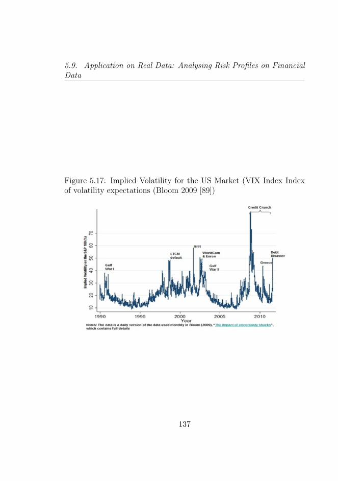
5.9. Application on Real Data: Analysing Risk Profiles on FinancialData
Figure 5.17: Implied Volatility for the US Market (VIX Index Indexof volatility expectations (Bloom 2009 [89])
137
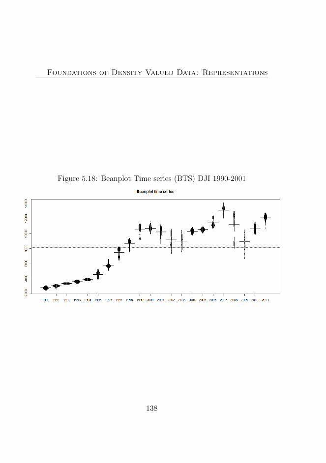
Foundations of Density Valued Data: Representations
Figure 5.18: Beanplot Time series (BTS) DJI 1990-2001
138
Part II
New Developments and NewMethods
139

Chapter 6
Visualization andExploratory Analysis ofBeanplot Data
In this chapter we propose a new approach for the aggregation, thevisualization and the analysis of the complex time series1 seen in Chap-ter 2. In particular, this approach is based entirely on a representationlike the density data2 or the beanplot data (Kampstra (2008) [416]).
Thus we are in the framework of Chapters 3, 4 and 5 where we triedto summarize our data by considering classical intra-period statisticalrepresentations. These types of new aggregated time series (Beanplottime series BTS) can be successfully used when there is an overwhelm-
1By now we adopt the definition of complex time series in Diday 2002 [214]who defines the complex time series and the adequate description of the subpe-riod: ”representing each time series by the histogram of its values or in describingintervals of time”. In this respect we consider the intra-period representations asgenuine representations of the phenomena
2Clearly the density data comes from the kernel density estimation seen inChapter 5
Visualization and Exploratory Analysis of BeanplotData
ing number of observations, for example in High Frequency financialdata (in particular we refer to the specific characteristics of these dataas presented in Chapter 2, see also Dacorogna et al. 2001 [163]). Inthese cases, it is not possible to visualize the data adequately and soit is necessary to maximize the information obtained by consideringanother intra-period representation3.A second reason to use these types of aggregate representations isthat they allow the ”uncertainty visualization” (Griethe Schumann2006 [326] Johnson 2004 [408] and Potter 2006 [564]) where in theoriginal data there are present: ”error, imprecision, lineage, subjectiv-ity, noise, etc”.4 It is possible to visualize the uncertainty adequatelyby considering some alternative representations which have been pro-posed in literature in recent years.As we showed in Chapter 2, there are important cases in complex data(for example, the financial time series) in which there is uncertainty,due to the structure of the data for example5 (errors, missing value,etc.)
A third reason can be considered to be the capacity of aggregaterepresentations to detect patterns in data. So, they can be useful foranalyzing the complex behaviour of the markets where we can dis-cover important patterns in the long time6. For example, these meth-ods can capture complex patterns of dependency over the time, whereit is known that financial markets show the example phenomena oflong time autocorrelation (see Cont [153], Muchnik, Bunde, & Havlin(2009) [519] and Henry Zaffaroni 2003 [358]). A similar result is ob-tained using the Histogram Data of Gonzales-Rivera and Arroyo 2011
3See Tufte 1983 [668]4Boller Braun Miles and Laidlaw 2010 [101]; for a different and opposing opinion
about the uncertainty visualization see Boukhelifa Duke 2009 [105]5See Brownlees and Gallo 2006 [115] but also Dacorogna et al. 2001 [161]6In particular, one of the reasons to use these types of representations is the
capability to analyse the long run dynamics of the complex time series
142
[318] which find some correlations between low values of the marketindex over time. In general the Econophysics approach analyses thecomplex behavior of the markets in the data7.
These types of complex dependencies on data could be analysed byconsidering the minima and the maxima of the beanplot time seriesBTS8. The beanplot time series BTS naturally represents the inter-nal variation and the uncertainty, whereas the stripchart (the internalobservation) reduces the information.9. It is important to note thatthe use of the beanplot enhances the possibility to compare a higherquantity of data, and so could be useful in the analysis of the risk overtime10
We present in this chapter a represention based on the beanplottime series BTS, of high frequency data, while in the next we proposea particular coefficient estimation (see Chapter 7) and we will use itfor the forecasting and clustering aims later in the work (Chapter 8and 9). In particular, we will show the usefulness of this approachin analysing the long run dynamics of the markets and the businesscycle.
This chapter is organized as follows: in the first part we approachthe economic problem and how it is possible to obtain density datatypes of data by starting from a different type of scalar data. In thethird part we present the beanplot or density data and we describe
7In recent years there has been the growth of many works that try to understandthe financial markets as complex systems, see Mantegna and Stanley 2000 a firstapproach into Econophysics [485] and for a view of the Financial Markets as realworld complex system see Johnson Jeffries Ming Hui 2003 [409]. On the criticismof the main classical economic models and for the search of a new paradigm seeMandelbrot Hudson 2006 [483]
8For example, it is interesting to analyse the complex characteristics in a finan-cial time series: see Cont 2001 [152] and Sewell 2008 [619]
9There are important reasons to choose the interval data in the analysis10For example in the analysis of Risk and Financial Risk it could be very im-
portant (see Resti Sironi 2007 [580]
143
Visualization and Exploratory Analysis of BeanplotData
their features. In the fourth part we introduce the beanplot time se-ries (BTS) and the possibility to gain new information with these typesof data from the characteristics of the scalar time series. In the fifthand the sixth parts we introduce the internal and the external mod-elling process, whilst in the Ninth Chapter we introduce the mixtureanalysis as a tool in the diagnostic internal modelling.
6.1 The Data Aggregation problem
In particular an (ordinal) scalar time series takes the form yt, t =1...T with yt ∈ < and can have a single value in <.
By considering more than one statistical unit yt,i, t = 1...T, i =1...I we can consider longitudinal data (time series cross sectionaldata)11. Usually cross sectional time series are different from the paneldata because here I is fixed and T tends to be large whereas in thepanel data case I is large and T is fixed.
There are real cases, in particular, in which scalar time series ytdoes not allow one to correctly approach a phenomena, in particularwhen the dataset contains a huge quantity of observations and theirvisualization is not possible (see figure 6.1 ). Another important casecould happen when we are interested not in a single value but in a spe-cific distribution of a variable K in a given temporal interval T (forexample, Arroyo and Mate (2006) [43] refer to the variable as out-comes of the daily time-varying demand of energy). In other works,Arroyo et al. (2011) [38] try to predict the histogram data over time12.
11Beck 2004 [69] shows a high quantity of examples of longitudinal data, all theseexamples are characterised by a higher quantity of information than ”normal”datasets
12In all these approaches, authors directly consider the Symbolic Data Analysisapproach as considered in Diday 2002 [206]
144
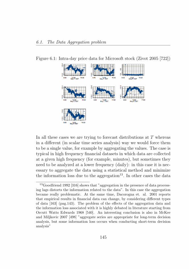
6.1. The Data Aggregation problem
Figure 6.1: Intra-day price data for Microsoft stock (Zivot 2005 [722])
In all these cases we are trying to forecast distributions at T whereasin a different (in scalar time series analysis) way we would force themto be a single value, for example by aggregating the values. The case istypical in high frequency financial datasets in which data are collectedat a given high frequency (for example, minutes), but sometimes theyneed to be analyzed at a lower frequency (daily): in this case it is nec-essary to aggregate the data using a statistical method and minimizethe information loss due to the aggregation13. In other cases the data
13Goodfriend 1992 [316] shows that ”aggregation in the presence of data process-ing lags distorts the information related to the data”. In this case the aggregationbecame really problematic. At the same time, Dacorogna et. al. 2001 reportsthat empirical results in financial data can change, by considering different typesof data [163] (pag.143). The problem of the effects of the aggregation data andthe information loss associated with it is highly debated in literature starting fromOrcutt Watts Edwards 1968 [540]. An interesting conclusion is also in McKeeand Miljkovic 2007 [498] ”aggregate series are appropriate for long-term decisionanalysis, but some information loss occurs when conducting short-term decisionanalysis”
145
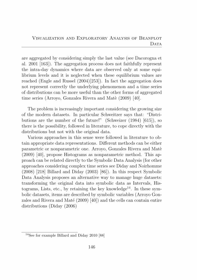
Visualization and Exploratory Analysis of BeanplotData
are aggregated by considering simply the last value (see Dacorogna etal. 2001 [163]). The aggregation process does not faithfully representthe intra-day dynamics where data are observed only at some equi-librium levels and it is neglected when these equilibrium values arereached (Engle and Russel (2004)[253]). In fact the aggregation doesnot represent correctly the underlying phenomenon and a time seriesof distributions can be more useful than the other forms of aggregatedtime series (Arroyo, Gonzales Rivera and Mate (2009) [40].
The problem is increasingly important considering the growing sizeof the modern datasets. In particular Schweitzer says that: “Distri-butions are the number of the future!” (Schweizer (1984) [615]), sothere is the possibility, followed in literature, to cope directly with thedistributions but not with the original data.
Various approaches in this sense were followed in literature to ob-tain appropriate data representations. Different methods can be eitherparametric or nonparametric one. Arroyo, Gonzales Rivera and Mate(2009) [40], propose Histograms as nonparametric method. This ap-proach can be related directly to the Symbolic Data Analysis (for otherapproaches considering complex time series see Diday and Noirhomme(2008) [218] Billard and Diday (2003) [86]). In this respect SymbolicData Analysis proposes an alternative way to manage huge datasets:transforming the original data into symbolic data as Intervals, His-tograms, Lists, etc., by retaining the key knowledge14. In these sym-bolic datasets, items are described by symbolic variables (Arroyo Gon-zales and Rivera and Mate (2009) [40]) and the cells can contain entiredistributions (Diday (2006)
14See for example Billard and Diday 2010 [88]
146
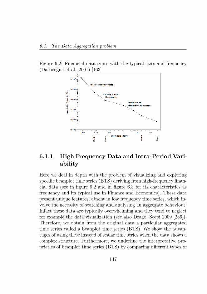
6.1. The Data Aggregation problem
Figure 6.2: Financial data types with the typical sizes and frequency(Dacorogna et al. 2001) [163]
6.1.1 High Frequency Data and Intra-Period Vari-ability
Here we deal in depth with the problem of visualizing and exploringspecific beanplot time series (BTS) deriving from high-frequency finan-cial data (see in figure 6.2 and in figure 6.3 for its characteristics asfrequency and its typical use in Finance and Economics). These datapresent unique features, absent in low frequency time series, which in-volve the necessity of searching and analysing an aggregate behaviour.Infact these data are typically overwhelming and they tend to neglectfor example the data visualization (see also Drago, Scepi 2009 [236]).Therefore, we obtain from the original data a particular aggregatedtime series called a beanplot time series (BTS). We show the advan-tages of using these instead of scalar time series when the data shows acomplex structure. Furthermore, we underline the interpretative pro-prieties of beanplot time series (BTS) by comparing different types of
147
Visualization and Exploratory Analysis of BeanplotData
aggregated time series. In particular, with simulated and real exam-ples, we will illustrate the different statistical performances of beanplottime series (BTS) in respect to boxplot time series (BoTS).
High-frequency financial data (Engle Russell 1998 [253]) are obser-vations on financial variables collected daily or at a finer time scale(such as time stamped transaction-by-transaction, tick-by-tick data,etc.). This type of data have been widely used to study various mar-ket microstructure related issues, including price discovery, compe-tition among related markets, strategic behaviour of market partici-pants, and modelling of real-time market dynamics. Moreover, high-frequency data are also useful for studying the statistical properties,volatility in particular, of asset returns at lower frequencies. The anal-ysis of these data is complicated for different reasons. We deal witha huge number of observations (”the average daily number of quotesin the USD/EUR spot market could easily exceed 20,000” see EngleRussell 2009 [255]), often spaced irregularly over time, with diurnalpatterns, price discreteness, and with a complex structure of depen-dence. The characteristics of these data do not allow the visualizationand exploration by the means of classical scalar time series. Further-more, it becomes very difficult to forecast data without defining anaggregate behaviour.
In this chapter we will introduce beanplot time series (BTS) withthe aim of synthesizing and visualizing high-frequency financial dataor, more in general, complex types of temporal data. In particular, wewill discuss their properties by proposing critical comparisons amongdifferent possible aggregated time series. After that, we will carryout several simulated examples (in section 6.7), starting from differ-ent models, different numbers of observations and different intervals ofaggregation to show how beanplot time series (BTS) tend to performbetter than boxplot time series (BoTS). Some interpretative rules aregiven in subsection 6.7.1. We have enriched our analysis by an ap-plication on real high frequency financial data where we show how
148
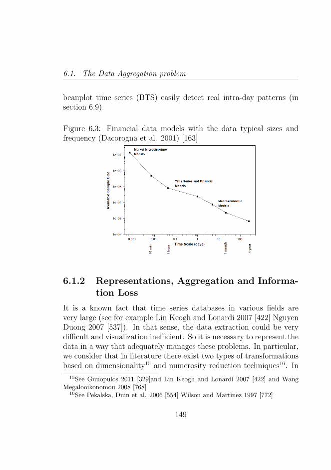
6.1. The Data Aggregation problem
beanplot time series (BTS) easily detect real intra-day patterns (insection 6.9).
Figure 6.3: Financial data models with the data typical sizes andfrequency (Dacorogna et al. 2001) [163]
6.1.2 Representations, Aggregation and Informa-tion Loss
It is a known fact that time series databases in various fields arevery large (see for example Lin Keogh and Lonardi 2007 [422] NguyenDuong 2007 [537]). In that sense, the data extraction could be verydifficult and visualization inefficient. So it is necessary to represent thedata in a way that adequately manages these problems. In particular,we consider that in literature there exist two types of transformationsbased on dimensionality15 and numerosity reduction techniques16. In
15See Gunopulos 2011 [329]and Lin Keogh and Lonardi 2007 [422] and WangMegalooikonomou 2008 [768]
16See Pekalska, Duin et al. 2006 [554] Wilson and Martinez 1997 [772]
149
Visualization and Exploratory Analysis of BeanplotData
this sense, the literature is very rich and symbolic representations17
are in this sense linked to two different approaches (Lin Keogh andLonardi 2007 [422]):
1. Data Adaptive
(a) Sorted Coefficients
(b) Piecewise Polynomial
(c) Singular Value Decomposition
(d) Symbolic
(e) Trees
2. Non Data Adaptive
(a) Wavelets
(b) Random Mappings
(c) Spectral
(d) Piecewise Aggregate Approximation
In that sense, as we have already seen, there is another approachwhich considers the problem of finding an adequate internal represen-tation of the variability.
In particular the same data, for each observation, can be consideredas characterized by internal variability as well (complex time series andhigh frequency data for example). In that case, data are not scalars
17Lin Keogh Lonardi Chiu (2003) [459]
150
6.1. The Data Aggregation problem
but are Intervals, Histograms, Boxplots etc.So, there are also cases where these internal representations are
interesting on their own (for example where there is the interest inmodelling the intra-period variability). In those cases we want to ex-plicitly analyse this variability.
More in general with the aim of summarizing and visualizing highfrequency time series, different types of statistical tools and aggregatedtime series can be considered18.
In particular, we can consider with respect to the problem of dataaggregation in complex time series these solutions:
1. Intervals
2. Boxplots
3. Histograms
4. Candlesticks
5. Beanplots
We define these as Complex Objects where in some cases they canbe defined as Temporal Symbolic Data (usually Symbolic Representa-tions are defined as the representation of time series using some othertypes of the methods seen above).
In practice we are trying to represent and to visualize the statisti-cal uncertainty by considering different Complex Objects (see Potter2006 [564]). In massive data sets the Data Analysis process can beconducted in two different ways: considering the original data usingthe classical temporal data mining techniques19 or the aggregate rep-resentations (or the Complex Objects).
18In all these cases we can use stripcharts, boxplots, histograms and so on19See for some overviews on the topic Laxman, Srivatsan, and P S Sastry. 2006
[441], Antunes and Oliveira 2001 [23] and Mitsa 2010 [510]
151
Visualization and Exploratory Analysis of BeanplotData
More generally identifying the data structure can be very relevantto understand the phenomenon from a statistical point of view20. Themean, the median, or the total of the single values represent weak ag-gregations because important information is neglected (see Marvasti2011 [489].
Initially, we used a stripchart time series (that could be relatedto the Interval Time Series (ITS): see Arroyo and Mate 2006 [43]).This type of time series correctly shows the original trend as well asthe minimum and the maximum of each interval (a day, for example).However in such graphics, one dot is plotted for each observation inthe single time interval and, consequently, it is a useful tool only whenthere are very few points.
Therefore, it might be difficult to apply them in the high frequencydata framework. A recent proposal (see Arroyo and Mate 2009 [44]and Arroyo et al.[37]), in the context of symbolic data, consists of sub-stituting time series of observations with histogram time series HTS(see Arroyo et al. 2011 [38]). These representations are very usefulfor temporal and spatial aggregations for many reasons: they are sim-ple with flexible structure, and they have the capacity to describe theessential features of the data with reasonable accuracy and with close-ness to the data, without imposing any distribution. Nevertheless, themultiple histograms are difficult to compare when there are many ofthem plotted on a graph, because the space becomes cluttered21.
Tukey’s boxplot (see Tukey 1977 [670]) is commonly used for com-
20Jackson 2008 [401] wrote ”The casual use of hypothesis tests based on arbitrarythresholds is frequently criticized (Gelman and Stern 2006 [294]), particularly inmedical research (Sterne et al. 2001 [642])”
21Another difficulty in using histograms is given by Elgammal et al. 2002 [246]:”The major drawback with color histograms is the lack of convergence to the rightdensity function if the data set is small. . . Unlike histograms, even with a smallnumber of samples, kernel density estimation leads to a smooth, continuous, anddifferentiable density estimate”.
152
6.1. The Data Aggregation problem
paring distributions between groups. For time series data, the boxplotseems to show several features of the temporal aggregation: center,spread, asymmetry and outliers. Furthermore, Box Plot time seriesdetect main structural changes well (Mate Arroyo 2006 [493]). How-ever the number of outliers detected will increase if the number of ob-servations grows and the information about the density is neglected.This information can be very important in the aggregation of highfrequency financial data where different volatility clusters can arise.
A way to visualize the data uncertainty related to the presence ofdifferent bumps by enhancing the initial boxplots is given by Hynd-man with the HDR boxplots (Hyndman 1996 [378]). Using these toolswe are able to identify the regions of highest density and so bumpscan occur in the density as well.
In order to retain this information, it is possible to use at the sametime the Violin Plot (see fig. 6.4) time series. This tool (Benjamini1988 [73]) combines the advantages of boxplots with the visualizationof the density and it provides a better indication of the shape of thedistribution. However, in a Violin Plot22 the underlying distribution isvisible but the individual points, besides the minimum and maximum,are not visible and no indication of the number of observations in eachgroup is given.
Other proposals related to the uncertainty in representations arecontained in Jackson (2008) [401] and Cleveland (1993) [146]. In par-ticular the first author makes a proposal related to the density strip,in which data are represented as a thin horizontal rectangle which isdarkest at the point of highest probability density, white at points ofzero density, and shaded with darkness proportional to the density23.In this case the relevant dimension is given by the shade of the image.
22There was in literature another proposal in this sense from Messing 2010 [815]that considers a single weight for each observation
23Jackson 2008 [401]
153
Visualization and Exploratory Analysis of BeanplotData
At the same time in violin plots there is not a specific visualizationof the single observations (so it is not possible to clearly identify theoutliers in data). Another proposal in literature is the Summary Plotby Potter Kniss Riesenfeld 2007 [565] in which we observe the density,the moments and the cumulant information
Other alternatives that use shading in visualizations to show densi-ties are in Cohen Cohen 2006 [148] using the Sectioned density plots.
Our proposal consists of using Beanplot time series -BTS (Kamp-stra 2008 [416]) in particular in the context of high frequency financialdata. Indeed, in each single beanplot all the individual observationsare visible as small lines in a one-dimensional scatter plot, as in astripchart24. In the Beanplot time series (BTS), both the averagefor each time interval (represented by the beanline) and the overallaverage is drawn; this allows for an easy comparison among tempo-ral aggregations. The estimated density of the distribution is visibleand this shows the existence of clusters in the data and highlights thepeaks, valleys and bumps. Furthermore, anomalies in the data, suchas bimodal distributions, are easily identified.
This is very interesting information in the context of high frequencyfinancial time series where the intra-period variability represents themain characteristics of the data. The number of bumps can be consid-ered as a signal of different market phases in the daily market struc-ture. We can also observe that the beanplot becomes longer in thepresence of price anomalies such as peculiar market behaviours (spec-ulative bubbles). See figures 6.4 and 6.5 for the different comparativeobject that could be used to represent the intra-period dynamics ofscalar complex time series. At the same time, in the following table wesummarize all the different complex objects that could be considered
24 Eklund 2010 [780] proposes a different tool like the beeswarm that can be con-sidered an improved stripchart where it is possible to visualize all the observation(experimentally on a limit of 1000-2000 observations)
154
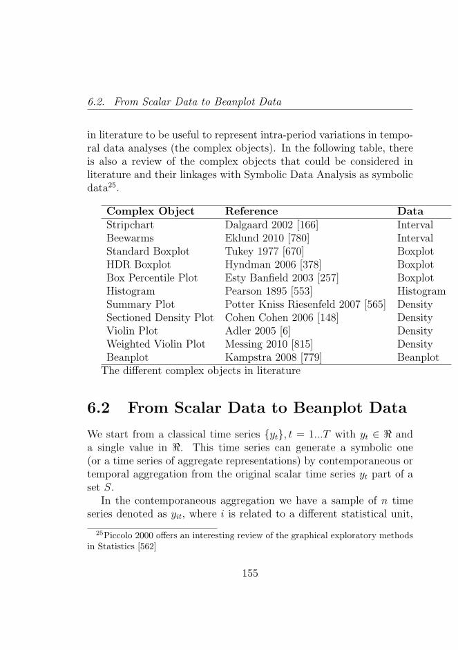
6.2. From Scalar Data to Beanplot Data
in literature to be useful to represent intra-period variations in tempo-ral data analyses (the complex objects). In the following table, thereis also a review of the complex objects that could be considered inliterature and their linkages with Symbolic Data Analysis as symbolicdata25.
Complex Object Reference DataStripchart Dalgaard 2002 [166] IntervalBeewarms Eklund 2010 [780] IntervalStandard Boxplot Tukey 1977 [670] BoxplotHDR Boxplot Hyndman 2006 [378] BoxplotBox Percentile Plot Esty Banfield 2003 [257] BoxplotHistogram Pearson 1895 [553] HistogramSummary Plot Potter Kniss Riesenfeld 2007 [565] DensitySectioned Density Plot Cohen Cohen 2006 [148] DensityViolin Plot Adler 2005 [6] DensityWeighted Violin Plot Messing 2010 [815] DensityBeanplot Kampstra 2008 [779] Beanplot
The different complex objects in literature
6.2 From Scalar Data to Beanplot Data
We start from a classical time series yt, t = 1...T with yt ∈ < anda single value in <. This time series can generate a symbolic one(or a time series of aggregate representations) by contemporaneous ortemporal aggregation from the original scalar time series yt part of aset S.
In the contemporaneous aggregation we have a sample of n timeseries denoted as yit, where i is related to a different statistical unit,
25Piccolo 2000 offers an interesting review of the graphical exploratory methodsin Statistics [562]
155
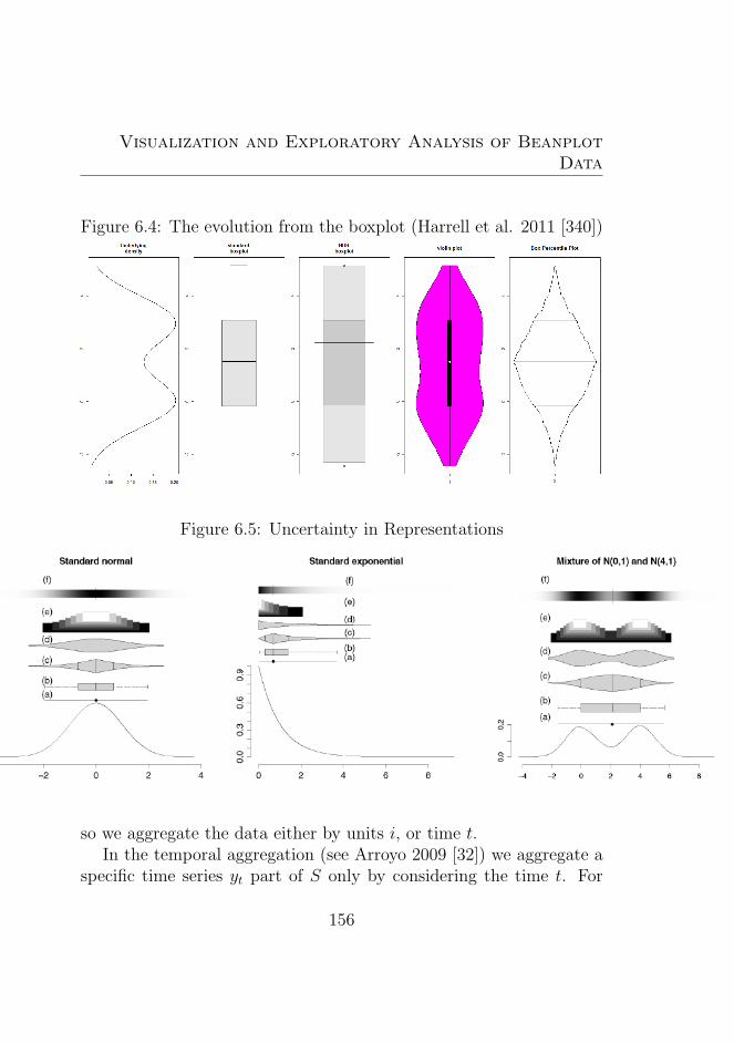
Visualization and Exploratory Analysis of BeanplotData
Figure 6.4: The evolution from the boxplot (Harrell et al. 2011 [340])
Figure 6.5: Uncertainty in Representations
so we aggregate the data either by units i, or time t.In the temporal aggregation (see Arroyo 2009 [32]) we aggregate a
specific time series yt part of S only by considering the time t. For
156
6.3. Beanplot Data
example, we can obtain as a symbolic time series a portfolio of stocksrelying on a specific criteria or sector (contemporaneous aggregation)or a financial high frequency time series considered at a lower frequency(temporal aggregation).
Definition 1. A primary data is an element xi in the set S. Asecondary data is a representation of the set S and they can be rep-resented as complex data (Billard and Diday 2006 [86]).
The statistical analysis can be conducted in two parallel ways: onprimary data (classical time series) and on the secondary data (thetime series representing portfolios, for example).
6.3 Beanplot Data
Following Arroyo, Gonzales-Rivera and Mate (2006), by taking intoaccount a variable X (for example the closing price of a stock) weconsider as primary, single observations part of a set S. For everyelement xi ∈ S we observe a secondary datum as a density.
Definition 2. A density data at time t is a representation of thexi single elements in the set S, such as from Chapter 5:
fh,t =1
nh
n∑i=1
K(x− xih
) (6.1)
where K is a Kernel and a h is a smoothing parameter defined as abandwidth. K can be a gaussian function with mean zero and variance1. The Kernel as we know is a non-negative and real-valued functionK(z) satisfying:
∫K(z)dz = 1,
∫zK(z)dz = 0,
∫z2K(z) = k2 < ∞
with the lower and upper limits of integration being −∞ and +∞.It is possible to use various Kernel functions (Ke): uniform, triangle,epanechnikov, quartic (biweight), tricube (triweight), gaussian andcosine. The variance can be controlled through the parameter h:
157
Visualization and Exploratory Analysis of BeanplotData
K(x− xih
) =1√2πe−
x−x2i
2h2 (6.2)
Various methods have been proposed in literature to choose thebandwidth h. Jones, Marron and Sheather (1996) proposed for exam-ple a bandwidth choice, based on the standard deviation:
hSNR = 1.06Sn−1/5 (6.3)
In the data visualization we use the Sheather-Jones criteria thatdefines the optimal h in a data-driven choice (Kampstra 2008).
Definition 3. A Beanplot data bYt is a combination of a 1-dscatterplot26 and a density trace (Kampstra 2008 [416]).
The beanplot can be considered as a particular case of interval-valued modal variable at the same time as boxplots and histograms(see Arroyo and Mate (2006)). In a beanplot we take into accountboth the interval between the minimum aLt , the maximum aUt andthe density as the kernel nonparametric estimator (the density trace,see Kampstra (2008)). Every single observation xit is represented onthe 1-dimensional scatterplot. This feature is useful to visually detectobservations distant from the others in the set S. The beanline attime t is a central measure of the beanplot (and a measure of locationof the object) and is defined as:
aMt =
∑ni=1(xit)
n(t = 1...T ) (6.4)
An alternative centre measure aMt is the median, where the quan-tiles can be considered in measuring the beanplots (in particular thesize of the object).
In the beanplot, the variability or size is mainly represented by the
26Dalgaard 2002 [166]
158
6.3. Beanplot Data
interval related to the minima aLt and the maxima aUt of X. The min-ima and the maxima localize as well the turning points in the originaltime series (in figure 6.6). The beanplot size can be represented inits data interval by [at] over the base set (E,≤) is the ordered pair[at] = [aLt , aUt ] where aLt , aUt ∈ E are the interval bounds such asaLt ≤ aUt . Inside the interval [aLt , aUt ] represent the single primaryobservations (represented as a 1-dimensional scatterplot or stripchart)so we are able to understand the location of the single observations inthe set S. The measure of size in the beanplot bYt is:
aSt = aUt − aLt (t = 1...T ) (6.5)
Where aUt is the upper bound and aLt is the lower bound.At the same time, it is possible to consider the interval composed by
the two consecutive sub-intervals (or half-point) through the beanline(the radii of the beanplot bYt): [a] = 〈aCt , aRt
〉 with:
aCt =(aUt + aLt)
2, aRt =
(aUt − aLt)
2(t = 1...T ) (6.6)
The interval arithmetic (Moore 1966 [513]) can be applied to bean-plot data.
So, why do we deal with beanplots? At this point we can give ananswer to this question: first of all beanplots permit the handling oflarge datasets, without deciding the number of the data features toimpose on data (in particular, bins).
At the same time beanplots can be used in two distinct ways, firstlyin an exploratory way to describe the underlying data structure (DragoScepi 2009 [236]), in particular beanplots tend to contain the informa-tion of the interval-value data, and the boxplot-value data. Secondly,beanplots can be used for the contained density trace which can be auseful tool in the analysis. It is possible in this sense to analyse andto forecast the intra-day dynamics without imposing a strong a-priori
159
Visualization and Exploratory Analysis of BeanplotData
hypothesis on the number of bins. At the same time the possibil-ity to visualize the observations can allow the quick identification ofthe outliers (a mechanism that is not permitted by using different datatypologies). Finally beanplots allow us to understand either the struc-tural changes due to breaks in the original time series or the changesdue to events to the series that create a change in the beanplot shape.
The kernel density estimators can be compared with other nonparametric methods of density estimation (see for example Fryer 1977[284]). Empirical results can show that, for example, the splines (seeAhlberg Nilson Walsh 1967 [8]) smooth out the original data. Thisimplied the loss of some relevant data features. Therefore, kernel den-sity estimators seem very useful in explorative contexts while splinesmoothers retain the very relevant data features, not taking into ac-count some irregularities which arise however, in this case of complexdata such as high frequency data.
The densities present characteristics which define well the structureof the data. In particular this structure can represent well at the sametime either the long run dynamics (the location of the data) or theintra-temporal variation (the size) that could be related in some spe-cific phenomena to the risk at time t. In general these types of datarepresent the single observation in a symbolic data table, where thesame symbolic data table can contain different types of data.
It is very important to observe the points of maxima density overtime t, in fact, these points represent the ”equilibrium” levels for eachtemporal observation at t. These equilibrium points represent valu-able information that is unknown or latent, related for example to theoccurrence of short term cycles and seasonalities.
160
6.4. Beanplot Time Series (BTS)
6.4 Beanplot Time Series (BTS)
Definition 4. A Time Series Beanplot bYt t = 1...T is an orderedsequence of beanplots or densities over the time.
Beanplots can be viewed as time series where they are realizationsof a X beanplot variable over the time t.
So at each time t we have different realizations of the interval-valuedata in the beanplot with the upper bound aUt and the lower boundaLt the beanline aCt and etc. So we obtain for each t the beanplotrealized stylized features for the location and the size:
[aU1 ; aC1 ; aL1 ] , [aU2 ; aC2 ; aL2 ] .... [aUt ; aCt ; aLt ] (6.7)
At the same time we obtain the descriptors for the beanlines overtime. The beanlines represent the location of the complex object. Sowe have:
[aM1 ] , [aM2 ] . . . [aMt ] (6.8)
At the same time, similarly to an interval we can obtain the radiiand the center for the beanplot. In that sense we obtain the descriptionof the dynamic of the size over time.
[aC1 ; aR1 ] , [aC2 ; aR2 ] . . . [aCt ; aRt ] (6.9)
A very important piece of information that needs to be provided isthe information on the first and the last observations in the temporalinterval. When the closing value is lower than the opening value itmeans that the original series is falling over time. We account also forthese descriptors over time.
[aOP1 ; aCL1 ] , [aOP2 ; aCL2 ] . . . [aOPt ; aCLt ] (6.10)
161
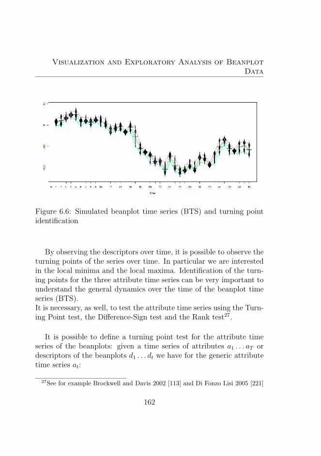
Visualization and Exploratory Analysis of BeanplotData
Figure 6.6: Simulated beanplot time series (BTS) and turning pointidentification
By observing the descriptors over time, it is possible to observe theturning points of the series over time. In particular we are interestedin the local minima and the local maxima. Identification of the turn-ing points for the three attribute time series can be very important tounderstand the general dynamics over the time of the beanplot timeseries (BTS).It is necessary, as well, to test the attribute time series using the Turn-ing Point test, the Difference-Sign test and the Rank test27.
It is possible to define a turning point test for the attribute timeseries of the beanplots: given a time series of attributes a1 . . . aT ordescriptors of the beanplots d1 . . . dt we have for the generic attributetime series at:
27See for example Brockwell and Davis 2002 [113] and Di Fonzo Lisi 2005 [221]
162
6.4. Beanplot Time Series (BTS)
at−1 < at and at > at+1 (6.11)
We obtain superior turning point, where the inferior one is:
at−1 > at and at < at+1 (6.12)
So there is a turning point if:
(at − at−1)(at+1 − at) < 0 (6.13)
The turning point test verifies if the observed series behave as ran-dom28. In that sense it is possible to show that:
tpn =pn − 2(n− 2)/3)√
16n− 29/90(6.14)
Where pn are the observed turning points. It is possible to showthat this value for n ≤ 25 tends to distribute as a standardized nor-mal. For the Difference Sign Test we check the different attribute timeseries:
Given dn as the number of differences (at−at−1). In the case E(Dn)on the hypothesis of random converge to:
tdn =dn − (n+ 1)/2√
(n+ 1/12)(6.15)
Another relevant test in that sense is the Rank Test29.It is possible also to consider the methods of analysis of the struc-
tural changes in the attribute time series at considered. It is interestingto note that structural change in the original time series correspondsto the structural change in one of these measures (or all together) as
28Brockwell and Davis 2002 [113] and Di Fonso Lisi 2005 [184]29Hallin and Puri 1992 [332] for a survey of the topic
163
Visualization and Exploratory Analysis of BeanplotData
minima, maxima and centre.Here we present the algorithm 2 for the classical analysis of the
beanplot time series (BTS) and the algorithm 3 for the analysis of thestructural change (see Zeileis et al. 2003 [713]).
In this sense, we can hypothesize to build different symbolic datatables using different intervals in which we compute densities overtime to discover these equilibrium points over the time (that could beuseful, for example in finance for trading purposes). A specific densityoriented type of data is the beanplot data [416], that considers jointlysome aspects of the underlying data (the value of the single data),as a specific stripchart diagram and the density in a form of densitytrace. A very interesting visualization is the data from the Dow Jonesindex computed for the period of the financial crisis, in figure 6.7 usingbeanplots data:
The stripchart diagram is very useful to detect the different intraperiod patterns in data. These different patterns can be due to sea-sonalities or intra-period cycles.In this sense the choice of the length of the single temporal interval t(day, month, year) is very important and depends on the specific datafeatures (the length of the cycles) and on the objectives the analystwants to study (Drago and Scepi 2009).
Another important point to consider in the beanplot time series(BTS) is the possibility of taking into account the first and the lastobservation of the beanplots to observe the intra-temporal dynamics(increasing values over time or not).
In figure 6.7 is the beanplot time series (BTS) for the Dow JonesMarket for the period 1996-2010, whilst in figure 6.8, figure 6.9 andfigure 7.0 there are the enhanced beanplot time series (BTS) consider-ing the first and the last observation for simulated and real data (DowJones Market and FTSEMIB Italian Market).
164
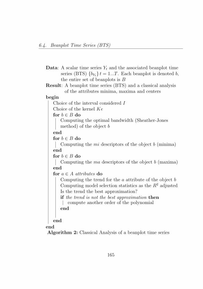
6.4. Beanplot Time Series (BTS)
Data: A scalar time series Yt and the associated beanplot timeseries (BTS) bYt t = 1...T . Each beanplot is denoted b,the entire set of beanplots is B
Result: A beanplot time series (BTS) and a classical analysisof the attributes minima, maxima and centers
beginChoice of the interval considered IChoice of the kernel Kefor b ∈ B do
Computing the optimal bandwidth (Sheather-Jonesmethod) of the object b
endfor b ∈ B do
Computing the mi descriptors of the object b (minima)endfor b ∈ B do
Computing the ma descriptors of the object b (maxima)endfor a ∈ A attributes do
Computing the trend for the a attribute of the object bComputing model selection statistics as the R2 adjustedIs the trend the best approximation?if the trend is not the best approximation then
compute another order of the polynomialend
end
endAlgorithm 2: Classical Analysis of a beanplot time series
165
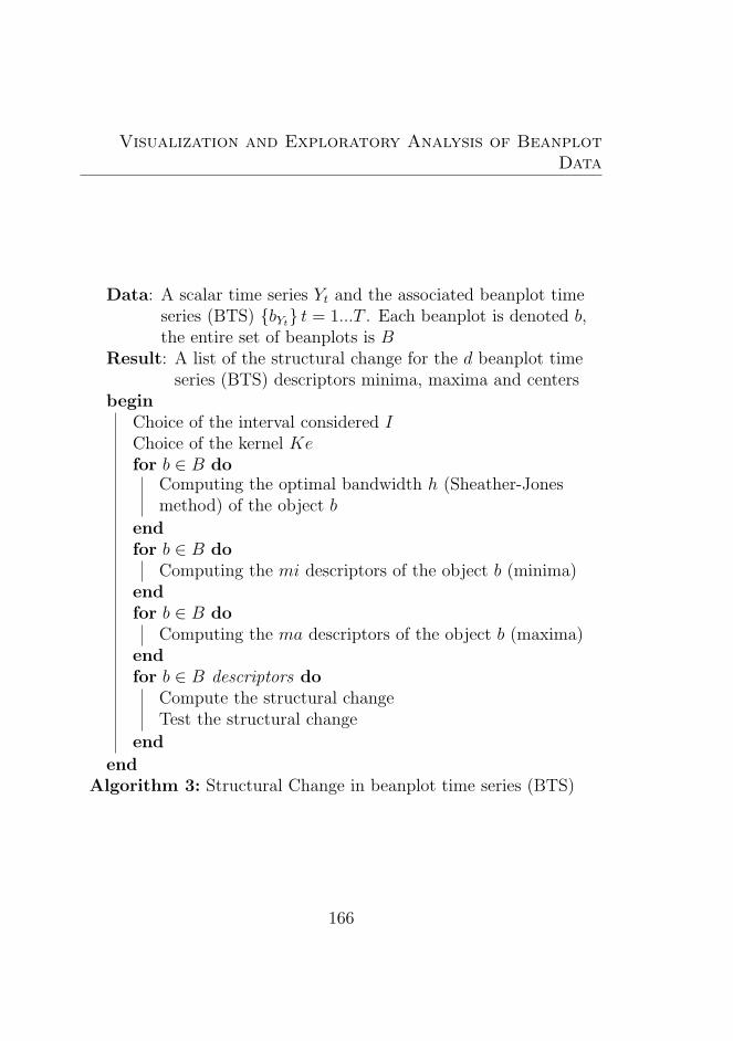
Visualization and Exploratory Analysis of BeanplotData
Data: A scalar time series Yt and the associated beanplot timeseries (BTS) bYt t = 1...T . Each beanplot is denoted b,the entire set of beanplots is B
Result: A list of the structural change for the d beanplot timeseries (BTS) descriptors minima, maxima and centers
beginChoice of the interval considered IChoice of the kernel Kefor b ∈ B do
Computing the optimal bandwidth h (Sheather-Jonesmethod) of the object b
endfor b ∈ B do
Computing the mi descriptors of the object b (minima)endfor b ∈ B do
Computing the ma descriptors of the object b (maxima)endfor b ∈ B descriptors do
Compute the structural changeTest the structural change
end
endAlgorithm 3: Structural Change in beanplot time series (BTS)
166
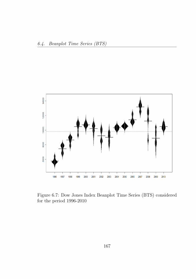
6.4. Beanplot Time Series (BTS)
Figure 6.7: Dow Jones Index Beanplot Time Series (BTS) consideredfor the period 1996-2010
167
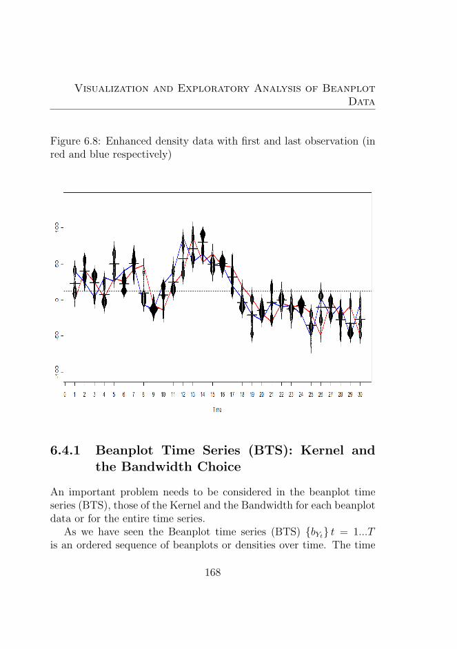
Visualization and Exploratory Analysis of BeanplotData
Figure 6.8: Enhanced density data with first and last observation (inred and blue respectively)
6.4.1 Beanplot Time Series (BTS): Kernel andthe Bandwidth Choice
An important problem needs to be considered in the beanplot timeseries (BTS), those of the Kernel and the Bandwidth for each beanplotdata or for the entire time series.
As we have seen the Beanplot time series (BTS) bYt t = 1...Tis an ordered sequence of beanplots or densities over time. The time
168
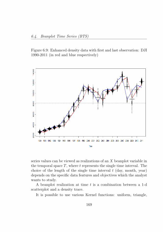
6.4. Beanplot Time Series (BTS)
Figure 6.9: Enhanced density data with first and last observation: DJI1990-2011 (in red and blue respectively)
series values can be viewed as realizations of an X beanplot variable inthe temporal space T , where t represents the single time interval. Thechoice of the length of the single time interval t (day, month, year)depends on the specific data features and objectives which the analystwants to study.
A beanplot realization at time t is a combination between a 1-dscatterplot and a density trace.
It is possible to use various Kernel functions: uniform, triangle,
169
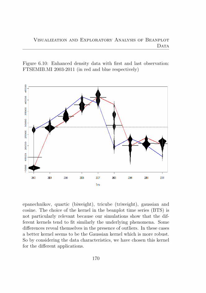
Visualization and Exploratory Analysis of BeanplotData
Figure 6.10: Enhanced density data with first and last observation:FTSEMIB.MI 2003-2011 (in red and blue respectively)
epanechnikov, quartic (biweight), tricube (triweight), gaussian andcosine. The choice of the kernel in the beanplot time series (BTS) isnot particularly relevant because our simulations show that the dif-ferent kernels tend to fit similarly the underlying phenomena. Somedifferences reveal themselves in the presence of outliers. In these casesa better kernel seems to be the Gaussian kernel which is more robust.So by considering the data characteristics, we have chosen this kernelfor the different applications.
170
6.4. Beanplot Time Series (BTS)
The choice of the h value is much more important than the choice ofK (see Silverman 1986) [633]. A large literature exists on bandwidthselection30. With small values of h, the estimate looks ”wiggly” andspurious features are shown. On the contrary, high values of h givea too smooth or too biased estimate and it may not reveal structuralfeatures, as for example the bimodality of the underlying density. Inany case it is difficult to give a clear indication of which bandwidthselection method is the best.
With a visualization aim, we use the Sheather-Jones criteria (SheatherJones 1991 [624]) that defines the optimal h in a data-driven approachin our application.
Here it is important to complete the part related to the beanplottime series (BTS) by focusing on the h choice of the same time series31.In fact it is important to note that where it is necessary to consider abeanplot time series (BTS) both for clustering or forecasting purposesit is necessary to fix one bandwidth for all beanplots (or for all thebeanplot time series BTS).
For visualization and strict data explorary purposes we can usea general bandwidth selection (the Sheather Jones method) for eachbeanplot data, but for other purposes it could be necessary to use an-other approach.
So we start from the original beanplot and we obtain the bandwidthwith the usual methods. The sequence of the values of the single band-width represents the level of variation of the beanplot. The value thatcould be chosen could be rationally chosen near the median by run-ning the algorithm 4 that visualizes the different beanplot time series
30In the multivariate case the research is less developed, see for example ZhangKing Hyndman 2004 [719] (see as surveys Marron 1987 [487]; Chiu 1991 [139];Jones, Marron and Sheather 1996 [413])
31This aspect is clearly not existent in the literature of interval time series (ITS),where it needs to be explored more in relation to the choice of the bins in theliterature of histogram time series (HTS)
171
Visualization and Exploratory Analysis of BeanplotData
(BTS) associated with the same algorithm.In any case the bandwidth of the different beanplot visualized over
time represents a useful indicator of the original data.
6.4.2 Trends, Cycles and Seasonalities
Definition 5. Beanplot Time Series (BTS) primary attributes arerealizations of a single beanplot bYt t = 1...T features over the time.
Primary attributes are related to the location and size of a beanplot.So we assume the aU1 , aC1 , aL1 to be composed of the components:
at = Trt + Cyt + Set + Act + Ut (6.16)
Where Tr is a trend component, Cy is a cycle, Se is a seasonality,andAc is an accidental component due to shocks, where U is a residual.
In this case we are assuming the mode:
at = f(t) + et (6.17)
for each attribute time series. Later we will consider also for timeseries, beanplot descriptors dt (or coefficients estimation).
Infact, by considering separately the aCt , aLt , aUt , we can computethe trend for each attribute time series, for example assuming thefunction f(t) as a polynomial (Di Fonzo Lisi 2005):
f(t) = δ0 + δ1t+ ...+ δqtq (6.18)
So we can estimate for each attribute time series aU1 , aC1 , aL1 as yt:
at = δ0 + δ1t+ ...+ δqtq + εt t = 1 . . . T ) (6.19)
We can express the 6.19 in this form:
172

6.4. Beanplot Time Series (BTS)
Data: A scalar time series Yt and the associated beanplot timeseries (BTS) bYt t = 1...T . Each beanplot is denotedbt, the entire set of beanplots is B
Result: a sequence of bandwidths h ∈ H related to thebeanplot Bt over time
beginChoice of the interval considered IChoice of the kernel Kfor b ∈ B do
Computing the optimal bandwidth (Sheather-Jonesmethod) of the object b
endIs it possible to use a criteria?if a criteria could be identified then
compute the bandwidth h for the beanplot time series(BTS)
end
Obtain a range of candidates of best bandwidth h(considering eventually the median)for h ∈ H bandwidths do
Visualize the bandwidth for each beanplot bVisualize the sequence of bandwidths
end
endAlgorithm 4: Choosing the optimal bandwidth
173
Visualization and Exploratory Analysis of BeanplotData
at = Dδ + ε (6.20)
Where D is a matrixWith:
a1
a2......an
=
1 t11 t21 . . . tm1
1 t12 t22 . . . tm2
1...
... . . ....
1...
... . . ....
1 t1n t2n . . . tmn
δ1
δ2......δn
+
ε1ε2......εn
(6.21)
y =
a1
a2
...an
, α =
δ0
δ1
...δn
, ε =
ε1ε2...εn
(6.22)
So by the Ordinary Least Squares we can obtain the estimates forthe parameters δ0, δ1...δq:
δ = (D′D)−1D
′y (6.23)
General rules of the scalar time series can be applied to select themodel for the trend (in particular the maximization of the R2) for eachattribute time series. A case of trend inadequacy is represented in thefigure 6.11. In the case represented in the figure it is necessary to useanother strategy in the trend estimation.
Before to consider the analysis of the cycle, it is interesting to notethat the beanplot time series (BTS) is a good tool for the analysis ofthe business cycle32, in fact they show the variability comparing the
32In particular they seem useful to be added to the classical tools of the BusinessCycle Analysis see Cipolletta (1992) [143]
174
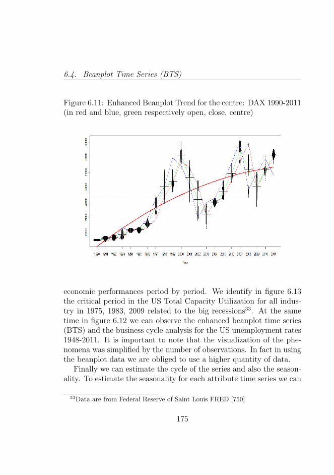
6.4. Beanplot Time Series (BTS)
Figure 6.11: Enhanced Beanplot Trend for the centre: DAX 1990-2011(in red and blue, green respectively open, close, centre)
economic performances period by period. We identify in figure 6.13the critical period in the US Total Capacity Utilization for all indus-try in 1975, 1983, 2009 related to the big recessions33. At the sametime in figure 6.12 we can observe the enhanced beanplot time series(BTS) and the business cycle analysis for the US unemployment rates1948-2011. It is important to note that the visualization of the phe-nomena was simplified by the number of observations. In fact in usingthe beanplot data we are obliged to use a higher quantity of data.
Finally we can estimate the cycle of the series and also the season-ality. To estimate the seasonality for each attribute time series we can
33Data are from Federal Reserve of Saint Louis FRED [750]
175
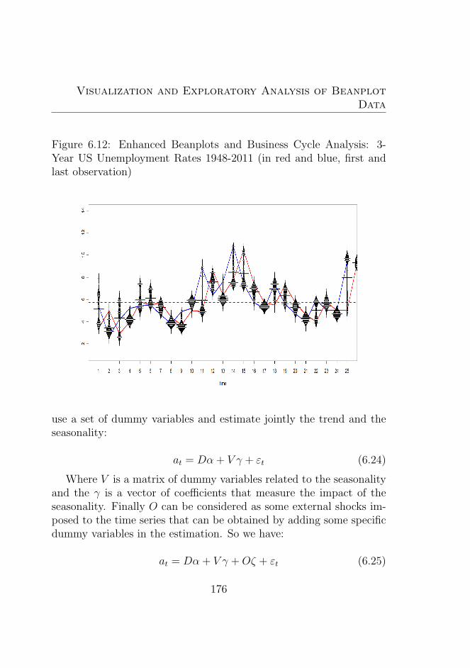
Visualization and Exploratory Analysis of BeanplotData
Figure 6.12: Enhanced Beanplots and Business Cycle Analysis: 3-Year US Unemployment Rates 1948-2011 (in red and blue, first andlast observation)
use a set of dummy variables and estimate jointly the trend and theseasonality:
at = Dα + V γ + εt (6.24)
Where V is a matrix of dummy variables related to the seasonalityand the γ is a vector of coefficients that measure the impact of theseasonality. Finally O can be considered as some external shocks im-posed to the time series that can be obtained by adding some specificdummy variables in the estimation. So we have:
at = Dα + V γ +Oζ + εt (6.25)
176
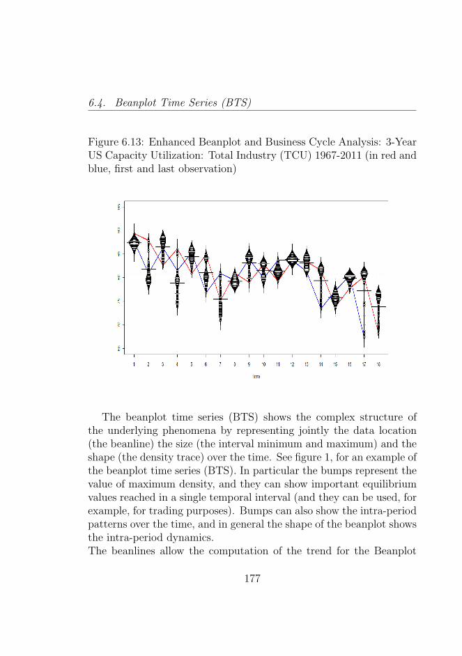
6.4. Beanplot Time Series (BTS)
Figure 6.13: Enhanced Beanplot and Business Cycle Analysis: 3-YearUS Capacity Utilization: Total Industry (TCU) 1967-2011 (in red andblue, first and last observation)
The beanplot time series (BTS) shows the complex structure ofthe underlying phenomena by representing jointly the data location(the beanline) the size (the interval minimum and maximum) and theshape (the density trace) over the time. See figure 1, for an example ofthe beanplot time series (BTS). In particular the bumps represent thevalue of maximum density, and they can show important equilibriumvalues reached in a single temporal interval (and they can be used, forexample, for trading purposes). Bumps can also show the intra-periodpatterns over the time, and in general the shape of the beanplot showsthe intra-period dynamics.The beanlines allow the computation of the trend for the Beanplot
177
Visualization and Exploratory Analysis of BeanplotData
time series (BTS). By choosing a suitable temporal interval it is pos-sible to visualize, as well, intra period seasonality patterns. More ingeneral, the beanplots seem to preserve the structure of the time se-ries, but show additional relevant patterns in data, for example byshowing bumps (or equilibrium levels over the time). Another impor-tant reason in using the beanplot is that these types of data can showlong-run structures where they can summarize a high quantity of dataover the time.
With respect to other complex objects or symbolic used in litera-ture, beanplots data are free to show the empirical structure for eachtemporal interval. At the same time we obtain a smoothed visualiza-tion of the underlying phenomena. Histograms and beanplots seemcomplementary: where histograms can be usefully compared, bean-plots tend to show the data structure, and they can show for exampleobservation that could be considered as outliers in a time series. Box-plot can be useful to detect and to identify outliers. In applications:histograms can be useful in setting trading systems whereas beanplotsseem to be very useful in risk management to analyze the occurrencesof financial crashes. In each case, it is easy to provide a transformationof the beanplot into other symbolic data. For example, it is very sim-ple to transform a beanplot time series (BTS) into an interval-valuedtime series (ITS).
6.5 Exploratory Data Analysis of Bean-
plot Time Series (BTS)
Following Shumway and Stoffer 2011 [629], by considering the beanplotextrema we are interested in exploring the data structure. We areinterested, in analysing, without any particular structural impositionthe dynamics over time of the beanplot structures, where they can
178
6.5. Exploratory Data Analysis of Beanplot Time Series (BTS)
show us the long run dynamics of both location, size and shape of thecomplex objects considered.
A moving average smoother mt can be useful for understanding andfor dividing the structure from the noise:
mt =k∑
j=−k
αjat−j (6.26)
Where: αj = α−j ≥ 0 and∑k
j=−k αj = 1In general it is used:
mt =k∑
j=−k
at−j2k + 1
(6.27)
Where wj =1
(2k + 1)In particular it is possible to average the observations using the
Kernel smoothing as a moving average smoother with a weight func-tion, or kernel. In particular we have:
ft =n∑i=1
wi(t)ai (6.28)
Where it is possible to consider:
wi(t) = K
(t−ib
)∑nj=1K
(t−jb
))
(6.29)
In which wi are specifically the weights, and K() is a kernel func-tion. It is possible to use the normal kernel:
K(z) =1√
2πexp(−z2/2)(6.30)
179
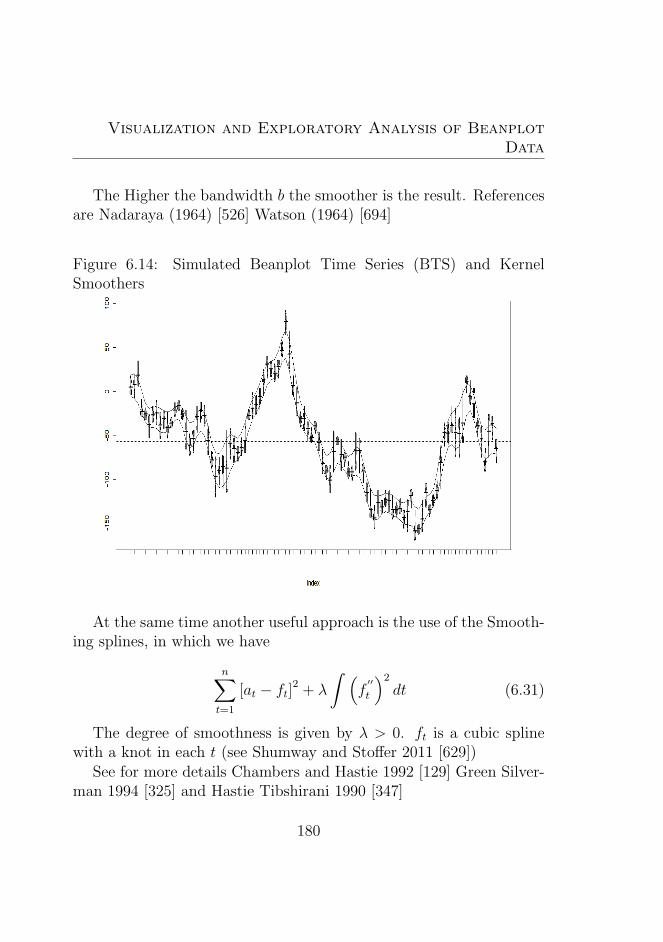
Visualization and Exploratory Analysis of BeanplotData
The Higher the bandwidth b the smoother is the result. Referencesare Nadaraya (1964) [526] Watson (1964) [694]
Figure 6.14: Simulated Beanplot Time Series (BTS) and KernelSmoothers
At the same time another useful approach is the use of the Smooth-ing splines, in which we have
n∑t=1
[at − ft]2 + λ
∫ (f′′
t
)2
dt (6.31)
The degree of smoothness is given by λ > 0. ft is a cubic splinewith a knot in each t (see Shumway and Stoffer 2011 [629])
See for more details Chambers and Hastie 1992 [129] Green Silver-man 1994 [325] and Hastie Tibshirani 1990 [347]
180
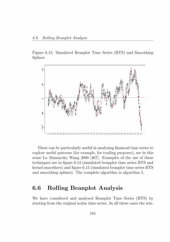
6.6. Rolling Beanplot Analysis
Figure 6.15: Simulated Beanplot Time Series (BTS) and SmoothingSplines
These can be particularly useful in analysing financial time series toexplore useful patterns (for example, for trading purposes), see in thissense Lo Mamaysky Wang 2000 [467]. Examples of the use of thesetechniques are in figure 6.14 (simulated beanplot time series BTS andkernel smoothers) and figure 6.15 (simulated beanplot time series BTSand smoothing splines). The complete algorithm is algorithm 5.
6.6 Rolling Beanplot Analysis
We have considered and analysed Beanplot Time Series (BTS) bystarting from the original scalar time series. In all these cases the win-
181
Visualization and Exploratory Analysis of BeanplotData
dow considered was specifically related to a specific temporal intervaldefined by the original data (as an aggregated data). In particularoriginal data could be daily, weekly, monthly, yearly etc. The actof considering a lower frequency can be useful for many importantreasons specifically linked to the analysis to be carried out. For ex-ample the risk analysis in financial data can be conducted on lowerfrequencies by taking into account a higher quantity of information,by considering a higher number of data available (in that case, theway to model risk is better).
Here, we consider Beanplot in a priori defined windows, where thewindows change over time by adding new data, in real time34. Wedefine this type of analysis Beanplot Rolling Analysis. In this sensethe window considered changes over time, where the window length isfixed. From the original Beanplot definition, we have (also Kampstra2008 [416]):
fh,t =1
nh
w∑i=1
K(x− xih
) (6.32)
where xi i = 1...w is the single observation in each t, K is a Kerneland a h is a smoothing parameter defined as a bandwidth. The windowi = 1 . . . varies over time by adding a new observation.
There are in this sense three approaches in the Beanplot RollingAnalysis which could be differently considered:
1. An overlapping approach (the data adjust observation by obser-vation)
2. A non overlapping approach (the windows are completely sepa-rated)
34These techniques are particularly relevant in a context where the financial dataare particularly volatile and the relationships can change over time (see PesaranTimmermann 2004 [558])
182
6.7. Beanplot Time Series (BTS) and Data Visualization: aSimulation Study
3. A partially overlapping approach (the data adjust by groups ofobservations)
Rolling Beanplot analysis is particularly useful in detecting thechange in data structure over time. A clearly important point hereis to detect a way to optimally consider the best temporal window.As will be seen later, the optimal strategy is to define the optimalwindow, using a number of observations of more than 30, to computethe density trace and to consider the cycle and choose the window insuch a way as to not hide the cycle of the original series.
6.7 Beanplot Time Series (BTS) and Data
Visualization: a Simulation Study
In order to study the performance of beanplot time series (BTS) invisualizing and exploring high frequency financial data we conduct sev-eral experiments on different models (Algorithm 6). The experimentsare designed to replicate different volatility processes (with increasingcomplexity). In this respect we study the capability of different aggre-gated time series (boxplot time series BoTS and beanplot time seriesBTS) to capture the main features of the original data.
18 types of models (GARCH/APARCH characterized by the mostsimple to the most complex different volatility structures). 10 repli-cations for each model. Each model contains characteristics of thefinancial time series such as volatility clusters, structural change, etc.200,000–700,000 observations aggregated in each beanplot temporalobservation. Comparing performances of different objects: Clustering(Hierarchical and PVclust) on the results, only with the descriptiveaim of comparing groups of objects
The Simulation Study Design algorithm: second stage
183
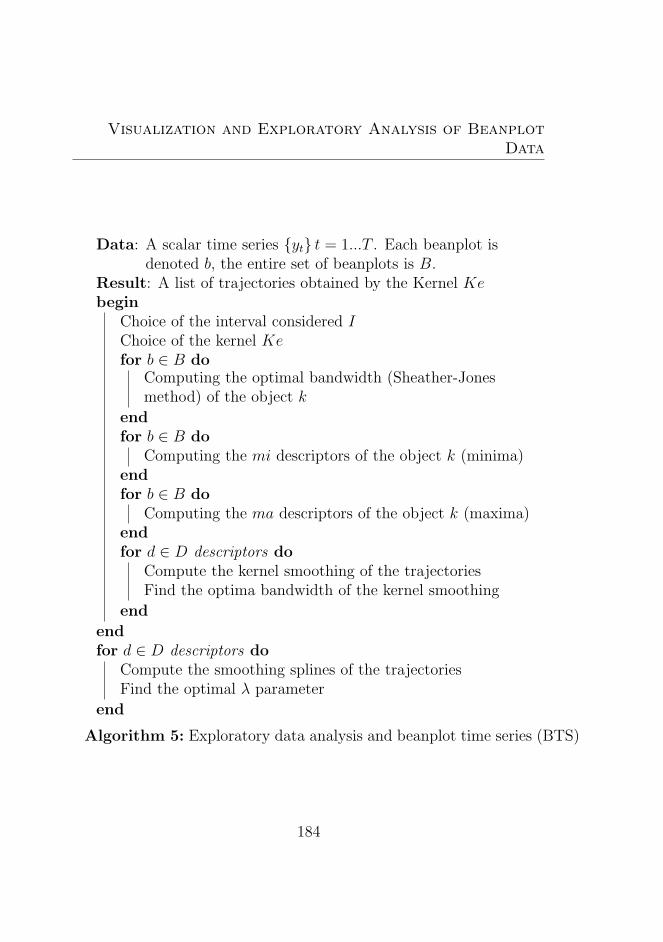
Visualization and Exploratory Analysis of BeanplotData
Data: A scalar time series yt t = 1...T . Each beanplot isdenoted b, the entire set of beanplots is B.
Result: A list of trajectories obtained by the Kernel Kebegin
Choice of the interval considered IChoice of the kernel Kefor b ∈ B do
Computing the optimal bandwidth (Sheather-Jonesmethod) of the object k
endfor b ∈ B do
Computing the mi descriptors of the object k (minima)endfor b ∈ B do
Computing the ma descriptors of the object k (maxima)endfor d ∈ D descriptors do
Compute the kernel smoothing of the trajectoriesFind the optima bandwidth of the kernel smoothing
end
endfor d ∈ D descriptors do
Compute the smoothing splines of the trajectoriesFind the optimal λ parameter
end
Algorithm 5: Exploratory data analysis and beanplot time series (BTS)
184
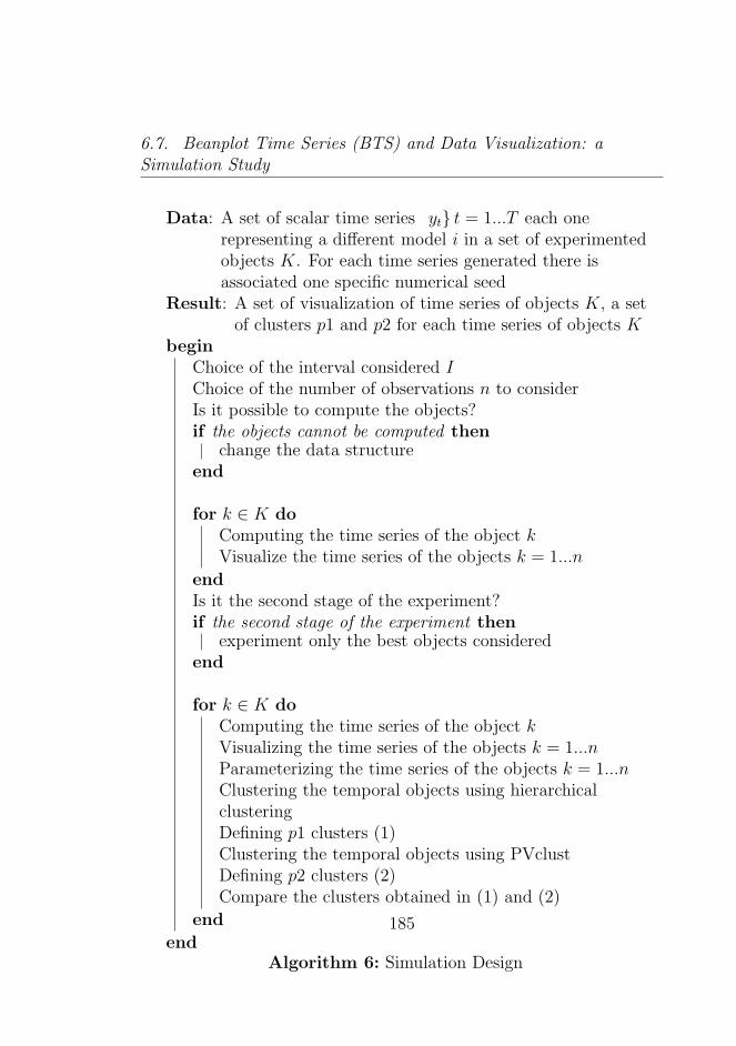
6.7. Beanplot Time Series (BTS) and Data Visualization: aSimulation Study
Data: A set of scalar time series yt t = 1...T each onerepresenting a different model i in a set of experimentedobjects K. For each time series generated there isassociated one specific numerical seed
Result: A set of visualization of time series of objects K, a setof clusters p1 and p2 for each time series of objects K
beginChoice of the interval considered IChoice of the number of observations n to considerIs it possible to compute the objects?if the objects cannot be computed then
change the data structureend
for k ∈ K doComputing the time series of the object kVisualize the time series of the objects k = 1...n
endIs it the second stage of the experiment?if the second stage of the experiment then
experiment only the best objects consideredend
for k ∈ K doComputing the time series of the object kVisualizing the time series of the objects k = 1...nParameterizing the time series of the objects k = 1...nClustering the temporal objects using hierarchicalclusteringDefining p1 clusters (1)Clustering the temporal objects using PVclustDefining p2 clusters (2)Compare the clusters obtained in (1) and (2)
end
endAlgorithm 6: Simulation Design
185
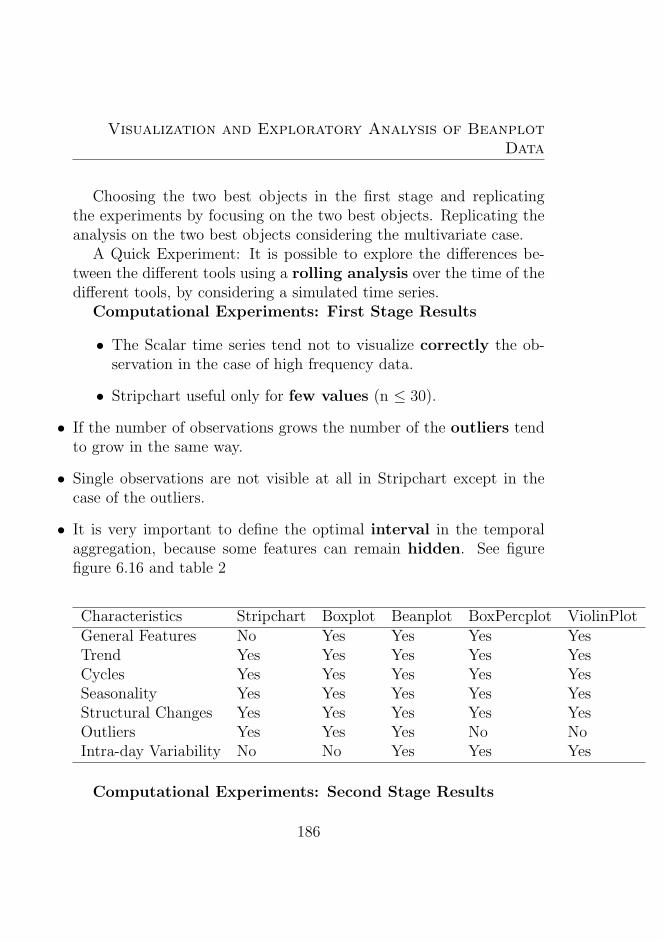
Visualization and Exploratory Analysis of BeanplotData
Choosing the two best objects in the first stage and replicatingthe experiments by focusing on the two best objects. Replicating theanalysis on the two best objects considering the multivariate case.
A Quick Experiment: It is possible to explore the differences be-tween the different tools using a rolling analysis over the time of thedifferent tools, by considering a simulated time series.
Computational Experiments: First Stage Results
• The Scalar time series tend not to visualize correctly the ob-servation in the case of high frequency data.
• Stripchart useful only for few values (n ≤ 30).
• If the number of observations grows the number of the outliers tendto grow in the same way.
• Single observations are not visible at all in Stripchart except in thecase of the outliers.
• It is very important to define the optimal interval in the temporalaggregation, because some features can remain hidden. See figurefigure 6.16 and table 2
Characteristics Stripchart Boxplot Beanplot BoxPercplot ViolinPlotGeneral Features No Yes Yes Yes YesTrend Yes Yes Yes Yes YesCycles Yes Yes Yes Yes YesSeasonality Yes Yes Yes Yes YesStructural Changes Yes Yes Yes Yes YesOutliers Yes Yes Yes No NoIntra-day Variability No No Yes Yes Yes
Computational Experiments: Second Stage Results
186
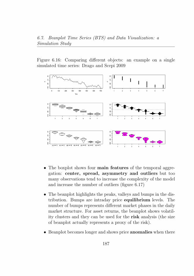
6.7. Beanplot Time Series (BTS) and Data Visualization: aSimulation Study
Figure 6.16: Comparing different objects: an example on a singlesimulated time series: Drago and Scepi 2009
• The boxplot shows four main features of the temporal aggre-gation: center, spread, asymmetry and outliers but toomany observations tend to increase the complexity of the modeland increase the number of outliers (figure 6.17)
• The beanplot highlights the peaks, valleys and bumps in the dis-tribution. Bumps are intraday price equilibrium levels. Thenumber of bumps represents different market phases in the dailymarket structure. For asset returns, the beanplot shows volatil-ity clusters and they can be used for the risk analysis (the sizeof beanplot actually represents a proxy of the risk).
• Beanplot becomes longer and shows price anomalies when there
187
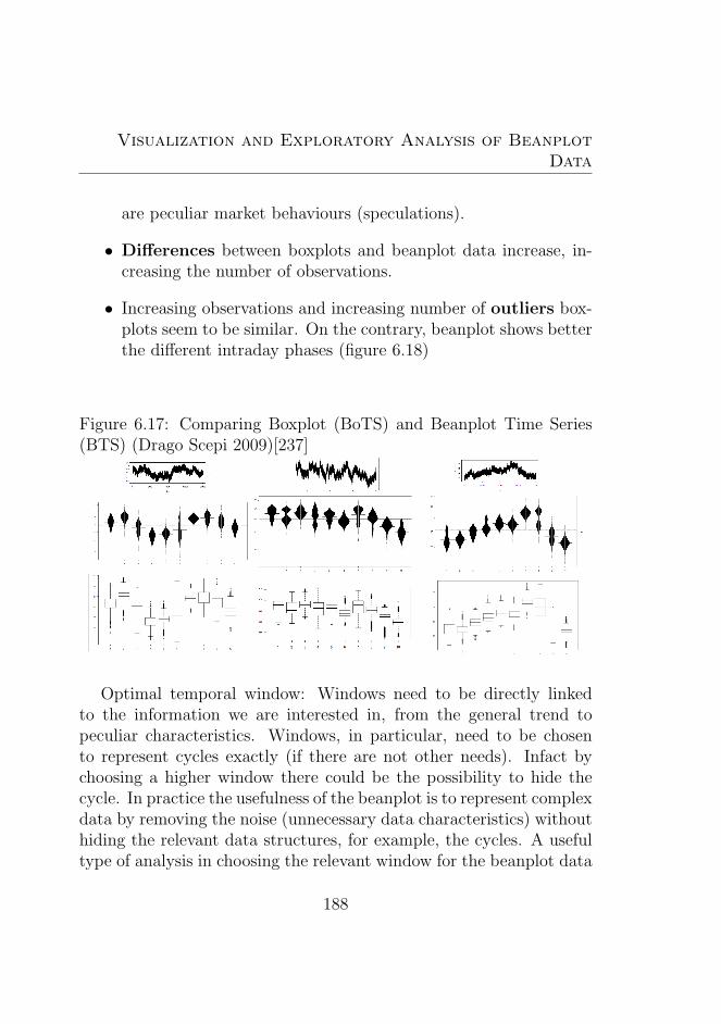
Visualization and Exploratory Analysis of BeanplotData
are peculiar market behaviours (speculations).
• Differences between boxplots and beanplot data increase, in-creasing the number of observations.
• Increasing observations and increasing number of outliers box-plots seem to be similar. On the contrary, beanplot shows betterthe different intraday phases (figure 6.18)
Figure 6.17: Comparing Boxplot (BoTS) and Beanplot Time Series(BTS) (Drago Scepi 2009)[237]
Optimal temporal window: Windows need to be directly linkedto the information we are interested in, from the general trend topeculiar characteristics. Windows, in particular, need to be chosento represent cycles exactly (if there are not other needs). Infact bychoosing a higher window there could be the possibility to hide thecycle. In practice the usefulness of the beanplot is to represent complexdata by removing the noise (unnecessary data characteristics) withouthiding the relevant data structures, for example, the cycles. A usefultype of analysis in choosing the relevant window for the beanplot data
188
6.7. Beanplot Time Series (BTS) and Data Visualization: aSimulation Study
could be the Spectral Analysis of a time series to define the length ofthe cycles (see Battaglia 2007 [66] and Hamilton 1994 [333]).
Figure 6.18: Comparing different interval temporal periods DragoScepi 2009 [237]
For our simulations we developed several algorithms in R. We gen-erated 18 types of models, where each model represents a differentunivariate GARCH/APARCH time series model
In order to analyse the effect of the different number of observationson our results, we varied, for each model, the number of observationsfrom 200,000 to 700,000. In this way, we simulated different typesof financial markets. Initially, we decided to aggregate our data inten different groups on ten different days. Then we tested differenttime aggregations (by reducing or increasing the number of groups).Therefore in each day we had from 20,000 to 70,000 observations.Finally, to test our results we made 100 replications for each model.
The outcome for each computational experiment performed is thevisualization of the different aggregated time series over the time. For
189
Visualization and Exploratory Analysis of BeanplotData
each experiment we registered the statistical features drawn from thebeanplot time series (BTS) compared to the original scalar time seriesand the boxplot time series (BoTS).
The results of our simulations show in the first place that the bean-plots tend to visualize a higher amount of information on the dailydata, and in particular the intra-day patterns in the behaviour of theseries, whereas the boxplots tend to return a smoothed view of thefinancial time series.
We report here, by way of example, the results with an underlyingmodel (model 1) of the type GARCH(1,1) and those obtained with amodel (model 2) of the type AR(1,5-GARCH(1,1) both with 200,000observations.
By increasing the complexity of the time series we observe moreclearly the differences between boxplot and beanplot time series (BTS).With beanplots, we are able to understand the structural changes andthe different forms of the objects more clearly. When the complexityreaches a very high level there is an increase of the outliers. Boxplottime series (BoTS) seem to suffer this higher volatility of the mar-kets. It is also interesting to note that by increasing the number ofobservations beanplots alone may give us clearer understanding andare therefore more useful than the boxplot time series (BoTS). In fact,the number of outliers tends to increase and the boxplots become sim-ilar to each other (in Fig. 6.17 we report an example of the modelwith 700,000 observations).
At the same time our simulations show that there is a specific num-ber of observations that could be retained by choosing one interval oranother. So the choice of the interval seems to be linked to the interestsof the researcher. In Fig. 6.18 we show the differences between bean-plot time series (BTS) with different temporal aggregations: a highernumber of observations considered in the interval shows a higher num-ber of bumps (and, of structural changes). The risk could be the lossof the information related to the cycles, where a lower number shows
190
6.7. Beanplot Time Series (BTS) and Data Visualization: aSimulation Study
the structure of the series, but it is expensive in terms of space used(and there is the risk of not visualizing patterns).
6.7.1 Some Empirical Rules of Interpretation
The aim of the analyst using the simulation is also to obtain someempirical rules of interpretation. The most important characteristicof the beanplot time series (BTS) is the capability to capture threerelevant aspects in the dynamics of the complex data: the location,the size, the shape. Therefore beanplot time series (BTS) should beinterpreted simultaneously considering this information.
The location shows the average or median price, and thus repre-sents a useful benchmark for comparing different units. This descrip-tor point gives the possibility to visualize a time series trend. Thisfeature is not possible with other smoothers or other nonparametrictechniques, while in the beanplot time series (BTS) we can explicitlyconsider a center for each time aggregation.
The size represents the general level of volatility, while the shapespecifically represents the internal structure and the intra-day pat-terns. Therefore, by observing these descriptor points, we can easilyidentify speculative bubbles, structural changes, market crashes, etc.Furthermore, beanplot bumps can be seen as equilibrium values forthe operators and they can be very important in trading strategies.
191
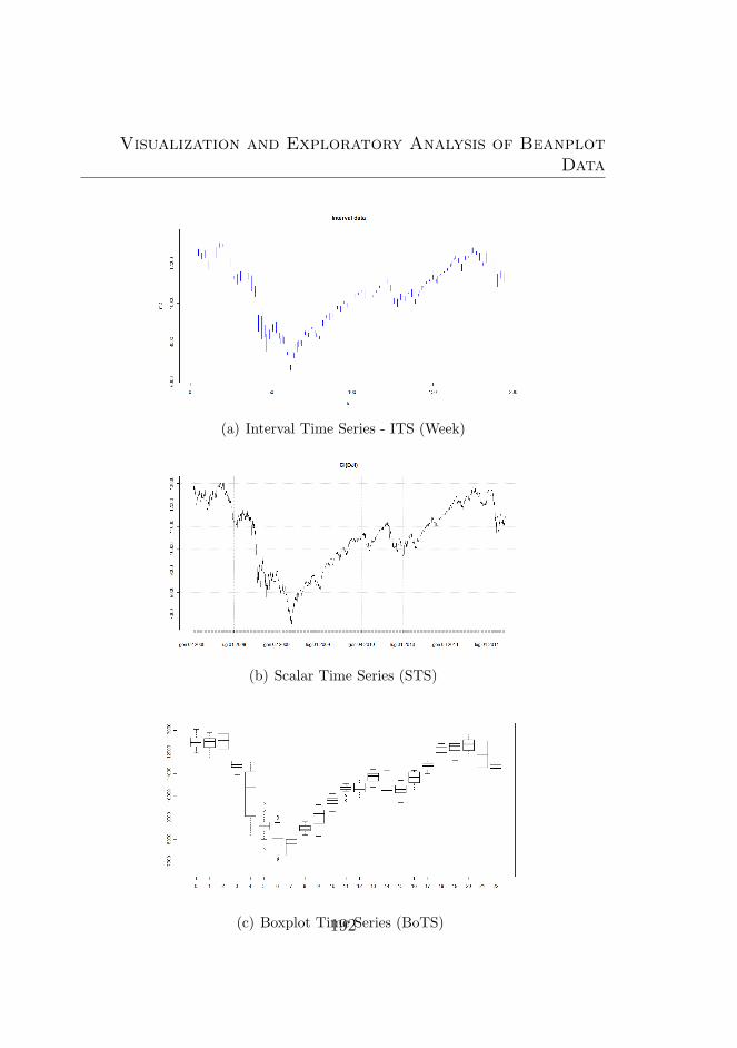
Visualization and Exploratory Analysis of BeanplotData
(a) Interval Time Series - ITS (Week)
(b) Scalar Time Series (STS)
(c) Boxplot Time Series (BoTS)192
6.8. Visualization: comparing the Beanplot time series (BTS) toother approaches
6.8 Visualization: comparing the Bean-
plot time series (BTS) to other ap-
proaches
An interesting experiment is now related to the use of real data (andthe associated problems of the choice of the interval temporal). Inparticular we look at the Dow Jones scalar time series in which weconsider the period related to the financial crisis 2008-2011. We con-sider comparatively the scalar time series (STS), the interval time se-ries (ITS), the boxplot time series (BoTS), the histogram (HTS) oneand the beanplot time series (BTS) (figure 6.18.2 and figure 6.18.3).
A first observation can be done in the choice of the week as anatural temporal interval for the intervals. The first impact on the vi-sualization shows that the different objects tend to visualize correctlythe most important features such as the cycles (the long run cyclesin particular) and the trend. It is chosen by considering the lengthof the cycle (so as to not eliminate its structure) by considering someinformation a priori. The interval time series (ITS) show the structureof the data, but in this case the problem of the number of the data canpersist. Choosing a lower temporal interval means we cannot observethe intra-period variation.
The boxplot can consider the interval (weekly), a higher temporalinterval, but the problem is that it tends to smooth the original dataand so not show the intra-period structural changes. At the same timethe relevant information is preserved.
The original scalar data normally show the structure of the data,but we are unable to observe all the observations in a good way, dueto the high number of data.
Using beanplot data we are able to observe the data, and in par-ticular we are able to observe the intra-period structural changes (thebumps).
193
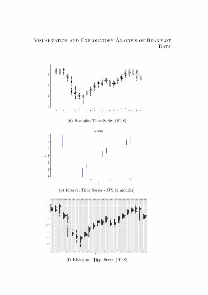
Visualization and Exploratory Analysis of BeanplotData
(d) Beanplot Time Series (BTS)
(e) Interval Time Series - ITS (2 months)
(f) Histogram Time Series (HTS)194
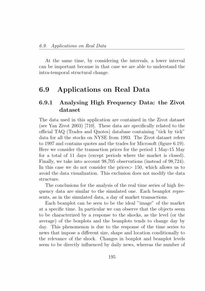
6.9. Applications on Real Data
At the same time, by considering the intervals, a lower intervalcan be important because in that case we are able to understand theintra-temporal structural change.
6.9 Applications on Real Data
6.9.1 Analysing High Frequency Data: the Zivotdataset
The data used in this application are contained in the Zivot dataset(see Yan Zivot 2003) [710]. These data are specifically related to theofficial TAQ (Trades and Quotes) database containing ”tick by tick”data for all the stocks on NYSE from 1993. The Zivot dataset refersto 1997 and contains quotes and the trades for Microsoft (figure 6.19).Here we consider the transaction prices for the period 1 May-15 Mayfor a total of 11 days (except periods where the market is closed).Finally, we take into account 98,705 observations (instead of 98,724).In this case we do not consider the prices> 150, which allows us toavoid the data visualization. This exclusion does not modify the datastructure.
The conclusions for the analysis of the real time series of high fre-quency data are similar to the simulated one. Each beanplot repre-sents, as in the simulated data, a day of market transactions.
Each beanplot can be seen to be the ideal ”image” of the marketat a specific time. In particular we can observe that the objects seemto be characterized by a response to the shocks, as the level (or theaverage) of the boxplots and the beanplots tends to change day byday. This phenomenon is due to the response of the time series tonews that impose a different size, shape and location conditionally tothe relevance of the shock. Changes in boxplot and beanplot levelsseem to be directly influenced by daily news, whereas the number of
195
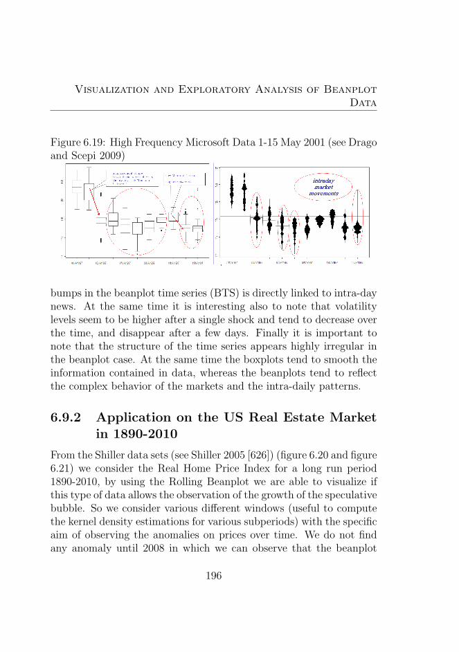
Visualization and Exploratory Analysis of BeanplotData
Figure 6.19: High Frequency Microsoft Data 1-15 May 2001 (see Dragoand Scepi 2009)
bumps in the beanplot time series (BTS) is directly linked to intra-daynews. At the same time it is interesting also to note that volatilitylevels seem to be higher after a single shock and tend to decrease overthe time, and disappear after a few days. Finally it is important tonote that the structure of the time series appears highly irregular inthe beanplot case. At the same time the boxplots tend to smooth theinformation contained in data, whereas the beanplots tend to reflectthe complex behavior of the markets and the intra-daily patterns.
6.9.2 Application on the US Real Estate Marketin 1890-2010
From the Shiller data sets (see Shiller 2005 [626]) (figure 6.20 and figure6.21) we consider the Real Home Price Index for a long run period1890-2010, by using the Rolling Beanplot we are able to visualize ifthis type of data allows the observation of the growth of the speculativebubble. So we consider various different windows (useful to computethe kernel density estimations for various subperiods) with the specificaim of observing the anomalies on prices over time. We do not findany anomaly until 2008 in which we can observe that the beanplot
196
6.9. Applications on Real Data
tends to show a strong change from the original series. Some valuescan be considered outliers, which mean that there was the growth of aspeculative bubble in the period (2007-2008). The result is confirmedby the fact that applying the rolling scalar time series, the DickeyFuller Test, we found that the series start to be non stationary in thesubperiod 210-240. At the same time an analysis on the structuralbreaks of the period show that there is a significant structural breakin the the second quarter of the year 2000.
Figure 6.20: Rolling Beanplots Real Home Price Index 1890-2011 usingdifferent windows
6.9.3 Comparing Instability and Long Run Dy-namics of the Financial Markets
We performed an analysis on some of the most relevant markets aroundthe world. The period considered are the years 1990-2011, where 2011is related to the period 1 January- 14 August. The missing data arenot considered. The analysis is divided into two phases:
197
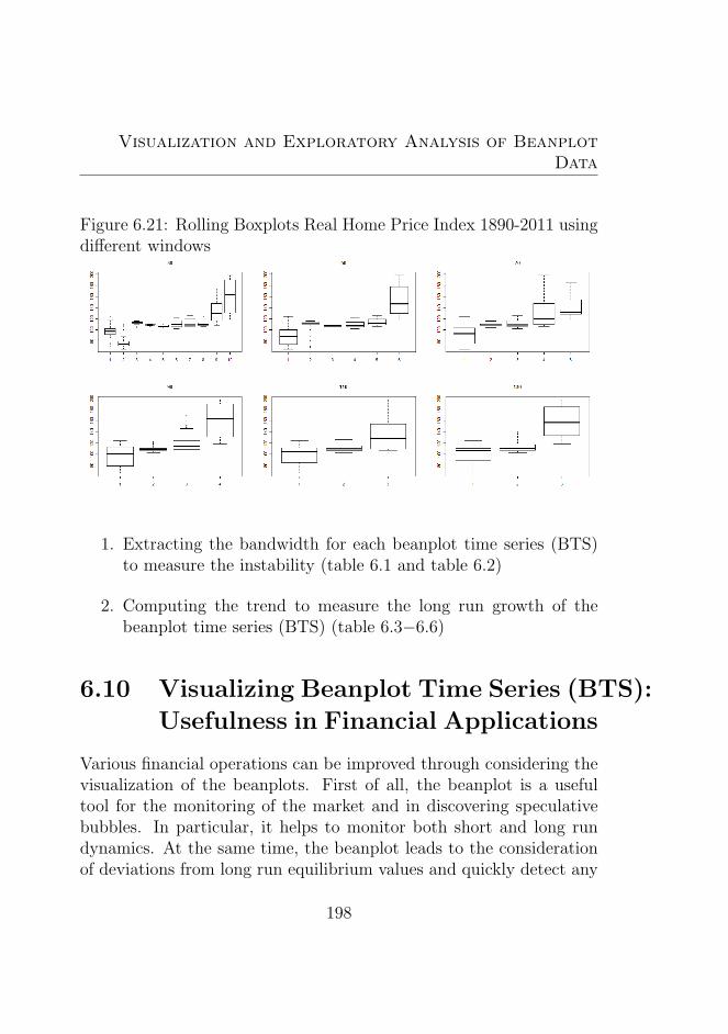
Visualization and Exploratory Analysis of BeanplotData
Figure 6.21: Rolling Boxplots Real Home Price Index 1890-2011 usingdifferent windows
1. Extracting the bandwidth for each beanplot time series (BTS)to measure the instability (table 6.1 and table 6.2)
2. Computing the trend to measure the long run growth of thebeanplot time series (BTS) (table 6.3−6.6)
6.10 Visualizing Beanplot Time Series (BTS):
Usefulness in Financial Applications
Various financial operations can be improved through considering thevisualization of the beanplots. First of all, the beanplot is a usefultool for the monitoring of the market and in discovering speculativebubbles. In particular, it helps to monitor both short and long rundynamics. At the same time, the beanplot leads to the considerationof deviations from long run equilibrium values and quickly detect any
198
6.10. Visualizing Beanplot Time Series (BTS): Usefulness inFinancial Applications
changes. These changes can be caused by structural factors (for ex-ample policies) which could change the beanplot structure. So, thebeanplot can be useful to monitor more than one stock at a time.Thus, it is useful in a asset allocation context, where it is necessaryto consider the performances of different stocks. In this sense, it ispossible to mix elements of the fundamental analysis and other finan-cial techniques to relate the outcomes from these techniques to thelocation, the size, and the shape of the beanplots. In this way it ispossible to anticipate the impacts of financial events on the beanplots.The capability of the tool to summarize a large quantity of informationcould be very useful in the monitoring of a large number of stocks. Vi-sualization is useful also in risk management techniques. In fact, it ispossible with the beanplot data to monitor the evolution of the identi-fied risks (also through using other techniques such as control charts).Here, the beanplot is useful also in the phase of scenario analysis asit is possible to consider and to use simulation methods to predict theimpact over time of different decisions and their outcomes. Beanplotsallow the visualization of the outcomes of many different economicpolicies in comparative scenarios.
Possible applications: Market Monitoring and discovering specula-tive bubbles, discovering financial market patterns (Statistical Arbi-trage), Asset Allocation, Risk Management, Scenario Analysis.
199
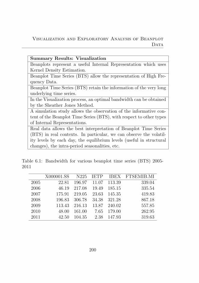
Visualization and Exploratory Analysis of BeanplotData
Summary Results: VisualizationBeanplots represent a useful Internal Representation which usesKernel Density Estimation.Beanplot Time Series (BTS) allow the representation of High Fre-quency Data.Beanplot Time Series (BTS) retain the information of the very longunderlying time series.In the Visualization process, an optimal bandwidth can be obtainedby the Sheather Jones Method.A simulation study allows the observation of the informative con-tent of the Beanplot Time Series (BTS), with respect to other typesof Internal Representations.Real data allows the best interpretation of Beanplot Time Series(BTS) in real contexts. In particular, we can observe the volatil-ity levels by each day, the equilibrium levels (useful in structuralchanges), the intra-period seasonalities, etc.
Table 6.1: Bandwidth for various beanplot time series (BTS) 2005-2011
X000001.SS N225 IETP IBEX FTSEMIB.MI2005 22.81 196.97 11.07 113.39 339.042006 46.19 217.08 19.49 185.15 335.542007 175.91 219.05 23.63 145.35 419.832008 196.83 306.78 34.38 321.28 867.182009 113.43 216.13 13.87 240.02 557.852010 48.00 161.00 7.65 179.00 262.952011 42.50 104.35 2.38 147.93 319.63
200
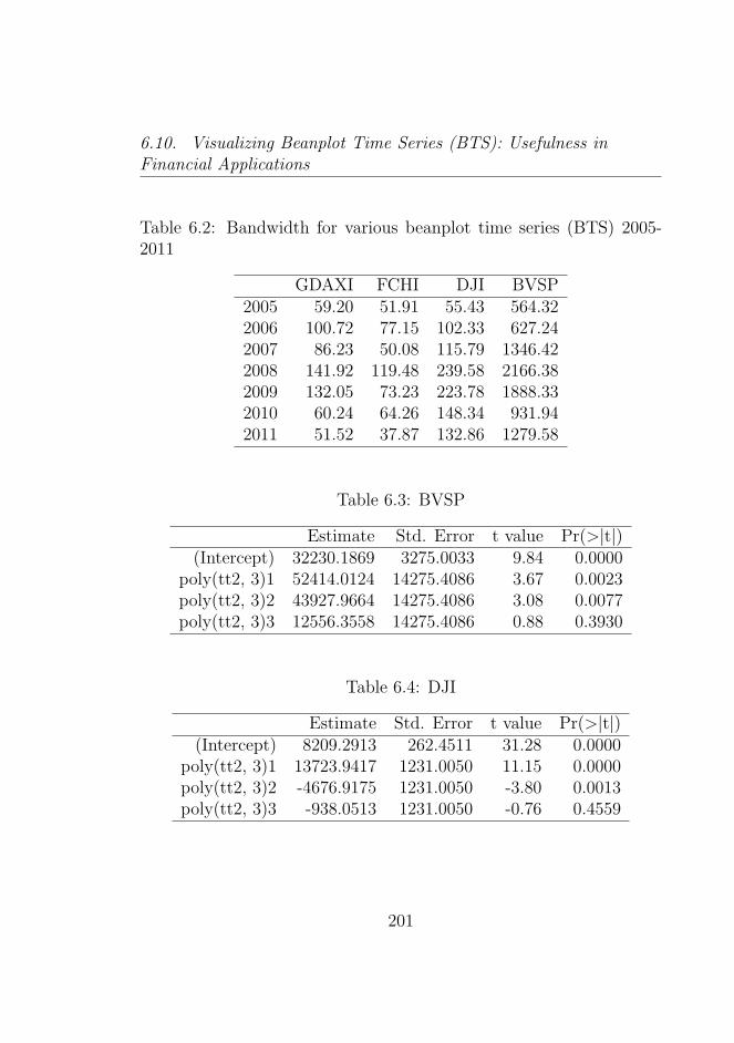
6.10. Visualizing Beanplot Time Series (BTS): Usefulness inFinancial Applications
Table 6.2: Bandwidth for various beanplot time series (BTS) 2005-2011
GDAXI FCHI DJI BVSP2005 59.20 51.91 55.43 564.322006 100.72 77.15 102.33 627.242007 86.23 50.08 115.79 1346.422008 141.92 119.48 239.58 2166.382009 132.05 73.23 223.78 1888.332010 60.24 64.26 148.34 931.942011 51.52 37.87 132.86 1279.58
Table 6.3: BVSP
Estimate Std. Error t value Pr(>|t|)(Intercept) 32230.1869 3275.0033 9.84 0.0000
poly(tt2, 3)1 52414.0124 14275.4086 3.67 0.0023poly(tt2, 3)2 43927.9664 14275.4086 3.08 0.0077poly(tt2, 3)3 12556.3558 14275.4086 0.88 0.3930
Table 6.4: DJI
Estimate Std. Error t value Pr(>|t|)(Intercept) 8209.2913 262.4511 31.28 0.0000
poly(tt2, 3)1 13723.9417 1231.0050 11.15 0.0000poly(tt2, 3)2 -4676.9175 1231.0050 -3.80 0.0013poly(tt2, 3)3 -938.0513 1231.0050 -0.76 0.4559
201
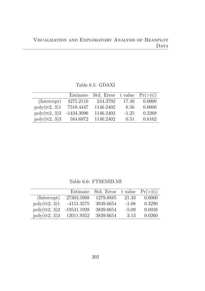
Visualization and Exploratory Analysis of BeanplotData
Table 6.5: GDAXI
Estimate Std. Error t value Pr(>|t|)(Intercept) 4275.2110 244.3792 17.49 0.0000
poly(tt2, 3)1 7518.4447 1146.2402 6.56 0.0000poly(tt2, 3)2 -1434.3096 1146.2402 -1.25 0.2268poly(tt2, 3)3 584.6972 1146.2402 0.51 0.6162
Table 6.6: FTSEMIB.MI
Estimate Std. Error t value Pr(>|t|)(Intercept) 27303.5908 1279.8885 21.33 0.0000
poly(tt2, 3)1 -4151.3575 3839.6654 -1.08 0.3290poly(tt2, 3)2 -19541.1928 3839.6654 -5.09 0.0038poly(tt2, 3)3 12011.9352 3839.6654 3.13 0.0260
202
Chapter 7
Beanplots Modelling
In this chapter we propose a new approach for modelling time seriesas complex data1, in particular financial data. For the new approach,in the same way as the works proposed by Arroyo 2009 [32] and Mate(2009) [491], the data is not scalar but is a representation of the intra-period variation as an interval, a histogram: in this case it is a densitythat presents interesting properties (Chapter 5). This type of data,can be clustered (Chapter 9) and forecasted (Chapter 8). The aim,in the present chapter, is that of modelling the variability of intra-period, that which relates to the temporal intervals. We define thesetypes of models as ”internal models” (see also Signoriello 2009 [630])and ”external models”, which are related to temporal dynamics.
In practice the idea is to reduce the errors related to the measure-ment error (see Rabinovich 1995 [568]), by considering a mathematicalmodel of the aggregated data2. Original data are infact characterizedby two distinct parts: the first, is structural and the second, is the
1Here we use the Diday definition of time series as complex data: see Diday2006 [208]
2In particular we model the original data as a density. See for mathematicalmodelling in this context Gershenfeld 1999 [295]
Beanplots Modelling
noise, which is influenced by many factors such as data incomplete-ness, errors, measurement errors, etc.3. Signoriello (2009) [630] alsoproposes this approach for histogram data4. In particular, the mod-elling approach (the internal model) is based, here, on the beanplotdata (Kampstra (2008) [416]) as already presented in Chapters 5 and6. These types of new aggregated time series can be fruitfully usedwhen there is an overwhelming number of observations, for example,in High Frequency financial data (this is different from other types ofaggregated data that do not faithfully represent the data structure).
The initial beanplot is explicitly modelled to permit the extrac-tion of the real data structure. At the same time we have seen inChapters 1 and 2 that there are cases in which data are overwhelmingand that using some aggregation can lead to a direct loss of informa-tion, for example in financial time series. These cases also determinemeasurement error, where original scalar data present errors (see howhigh frequency financial data contains errors in Dacorogna et al. 2001[163] and also Brownlees and Gallo 2006 [115]). In particular, highfrequency financial data shows some relevant characteristics (they areinequally spaced and contain errors), which suggest the use of somealternative methods like internal representations5 and the modellingpresented here. In this sense we have considered the use of the bean-plot, or density data (Kampstra 2008 [416]) in Drago Scepi 2009 [236]that summarizes the initial data through returning the relevant data
3See in this sense the introduction to the workshop Knemo in 2006 in Naplesthat shows the idea of this chapter very well [1]
4”According to the classical theory of measure, the data generated by the ”cor-rect model” are more ”real” than the empirical one, because they are purified fromerror sampling and from error of measurement. We should never forget that thereare no ”real” models, but rather models that approximate the reality in a more orless accurate manner..” Signoriello 2009 [630]
5Here we use the same term used by Lin Keogh Li and Lonardi 2007 [422] wherethe methods used are different because we represent the initial data as a density(whereas in the literature intervals, histograms etc. are used)
204
features. It is important to note that the beanplot time series (BTS)presented in Chapter 6, considers not only the extreme values of theinterval period but examines above all the intra-day dynamics6. Inthis case it could be relevant to take into account the structural partof the model and the noise related to the different density traces (asseen in Chapter 6).
In practice we propose a transformation of the original time seriesinto a density time series in order to analyse the variability intra-dayover time where it is necessary to extract the structural part from thenoise. The advantage of the approach can be seen by the fact thatit retains all the relevant information of the initial data in the den-sity plots and yet avoids the errors contained in the original data7.The coefficients estimation and the descriptor points will substitutethe original data, and the original beanplots as well. This approachallows us to take into account not only the aggregated values of thedata, but also8, the entire intra-day variation. The visualization ofthe beanplot time series (BTS) gives us the opportunity to retain allthe relevant information9.
6See for different methodological approaches and examples Mate 2009 [491] andArroyo, Espınola, Mate 2011 [36] Maia, De Carvalho, Ludermir 2008 [476] Arroyoet al. 2010 [39]
7It is important to stress that where the financial data are an excellent exampleof data that present a noise (see in that sense Sewell 2008 [619]), at the same timeother data types contain errors
8In high frequency data the last observation could also be considered: seeDacorogna et al. 2001 [163]
9The information can be related to the location, size and shape of the aggre-gated data (see Drago Scepi 2010 [236] and Drago Scepi 2010 [237]
205
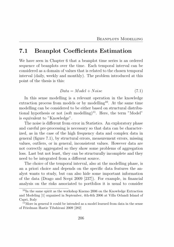
Beanplots Modelling
7.1 Beanplot Coefficients Estimation
We have seen in Chapter 6 that a beanplot time series is an orderedsequence of beanplots over the time. Each temporal interval can beconsidered as a domain of values that is related to the chosen temporalinterval (daily, weekly and monthly). The problem introduced at thispoint of the thesis is this:
Data = Model +Noise (7.1)
In this sense modelling is a relevant operation in the knowledgeextraction process from models or by modelling10. At the same timemodelling can be considered to be either based on structural distribu-tional hypothesis or not (soft modelling)11. Here, the term ”Model”is equivalent to ”Knowledge”.
The noise is different from error in Statistics. An exploratory phaseand careful pre-processing is necessary so that data can be character-ized, as in the case of the high frequency data and complex data ingeneral (figure 7.1), by structural errors, measurement errors, missingvalues, outliers, or in general, inconsistent values. However data arenot correctly aggregated so they show some problems of aggregationloss. Last but not least, they can be structurally incomplete and theyneed to be integrated from a different source.
The choice of the temporal interval, also at the modelling phase, isan a priori choice and depends on the specific data features the an-alyst wants to study, but can also hide some important informationof the data (Drago and Scepi 2009 [237]). For example, in financialanalysis on the risks associated to portfolios it is usual to consider
10In the same spirit as the workshop Knemo 2006 on the Knowledge Extractionand Modeling [1] organised in September, 4th-6th 2006 at Villa Orlandi Island ofCapri, Italy
11More in general it could be intended as a model learned from data in the senseof Friedman Hastie Tibshirani 2009 [282]
206
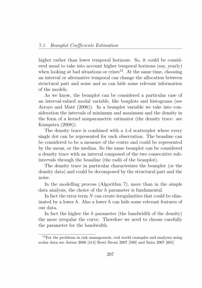
7.1. Beanplot Coefficients Estimation
higher rather than lower temporal horizons. So, it could be consid-ered usual to take into account higher temporal horizons (say, yearly)when looking at bad situations or crises12. At the same time, choosingan interval or alternative temporal can change the allocation betweenstructural part and noise and so can hide some relevant informationof the models.
As we know, the beanplot can be considered a particular case ofan interval-valued modal variable, like boxplots and histograms (seeArroyo and Mate (2006)). In a beanplot variable we take into con-sideration the intervals of minimum and maximum and the density inthe form of a kernel nonparametric estimator (the density trace: seeKampstra (2008)).
The density trace is combined with a 1-d scatterplot where everysingle dot can be represented for each observation. The beanline canbe considered to be a measure of the centre and could be representedby the mean, or the median. So the same beanplot can be considereda density trace with an interval composed of the two consecutive sub-intervals through the beanline (the radii of the beanplot).
The density trace in particular characterizes the beanplot (or thedensity data) and could be decomposed by the structural part and thenoise.
In the modelling process (Algorithm 7), more than in the simpledata analysis, the choice of the h parameter is fundamental.
In fact the error term N can create irregularities that could be elim-inated by a lower h. Also a lower h can hide some relevant features ofour data.
In fact the higher the h parameter (the bandwidth of the density)the more irregular the curve. Therefore we need to choose carefullythe parameter for the bandwidth.
12For the problems in risk management, real world examples and analyses usingscalar data see Jorion 2006 [414] Resti Sironi 2007 [580] and Saita 2007 [601]
207
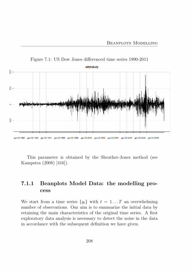
Beanplots Modelling
Figure 7.1: US Dow Jones differenced time series 1990-2011
This parameter is obtained by the Sheather-Jones method (seeKampstra (2008) [416]).
7.1.1 Beanplots Model Data: the modelling pro-cess
We start from a time series yt with t = 1 . . . T an overwhelmingnumber of observations. Our aim is to summarize the initial data byretaining the main characteristics of the original time series. A firstexploratory data analysis is necessary to detect the noise in the datain accordance with the subsequent definition we have given.
208
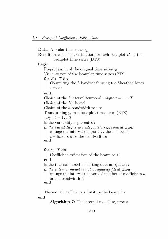
7.1. Beanplot Coefficients Estimation
Data: A scalar time series ytResult: A coefficient estimation for each beanplot Bt in the
beanplot time series (BTS)begin
Preprocessing of the original time series ytVisualization of the beanplot time series (BTS)for B ∈ T do
Computing the h bandwidth using the Sheather Jonescriteria
endChoice of the I interval temporal unique t = 1 . . . TChoice of the Ke kernelChoice of the h bandwidth to useTransforming yt in a beanplot time series (BTS)BYt t = 1 . . . TIs the variability represented?if the variability is not adequately represented then
change the interval temporal I, the number ofcoefficients n or the bandwidth h
end
for t ∈ T doCoefficient estimation of the beanplot Bt
endIs the internal model not fitting data adequately?if the internal model is not adequately fitted then
change the interval temporal I number of coefficients nor the bandwidth h
end
The model coefficients substitute the beanplots
endAlgorithm 7: The internal modelling process
209
Beanplots Modelling
We identify the outliers13 in the series yt, by using statisticalprocedures and adequate tests like the Dixon test for example.
In particular in high frequency time series the cleaning process ofthe time series is not needed. We perform, as well, the eventual trans-formations of the time series.
We substitute the initial data with the different subperiods rep-resented as Beanplots Ybt with t = 1...T . Subsequently we visualizethese subperiods of the series by means of a beanplot time series(BTS) considering a unique bandwidth for the BY t (Drago and Scepi2008).
By choosing a different interval it is possible to obtain a differentbeanplot structure, but the general features of the initial timeseries (trends, cycles, structural changes etc.) tend to be preserved.In general it is important to visualize adequately the original data inthe form of beanplot time series (BTS) and compute the bandwidth bymeans of the Sheather Jones method14. Secondly we can use this in-formation to compute a unique bandwidth for the entire series, (usingthe median of the bandwidths). Therefore we decide to define a propert temporal interval (say, daily, monthly etc.) so as to aggregate ourobservations. We substitute the initial data with the aggregated timeseries st with t = 1...T . Subsequently we visualize this aggregatedtime series by means of a beanplot time series (BTS) Bt (Drago Scepi2010 [237]). This allows us to represent the location (or the centre),the size and in particular the intra-period variability, which is not somanifest in the original time series.
By choosing a suitable temporal interval it is possible to visualize,as well, intra period seasonality patterns. In general, the beanplots
13 The identification of the outliers is relevant because they can have an impacton the results of the analysis based on scalar data: see Chalabi and Wurtz (2009)[128]
14That represent a curve rougher (an h higher) than another smoother one (witha lower h). See in this sense Wand and Jones 1995 [687]
210
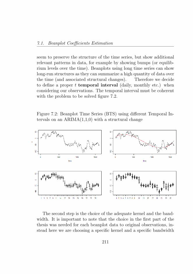
7.1. Beanplot Coefficients Estimation
seem to preserve the structure of the time series, but show additionalrelevant patterns in data, for example by showing bumps (or equilib-rium levels over the time). Beanplots using long time series can showlong-run structures as they can summarize a high quantity of data overthe time (and associated structural changes). Therefore we decideto define a proper t temporal interval (daily, monthly etc.) whenconsidering our observations. The temporal interval must be coherentwith the problem to be solved figure 7.2.
Figure 7.2: Beanplot Time Series (BTS) using different Temporal In-tervals on an ARIMA(1,1,0) with a structural change
The second step is the choice of the adequate kernel and the band-width. It is important to note that the choice in the first part of thethesis was needed for each beanplot data to original observations, in-stead here we are choosing a specific kernel and a specific bandwidth
211
Beanplots Modelling
for all the observations.For the choice of the unique bandwidth for the entire series, vari-
ous methods can be used in order to define the best one in advance:Jones, Marron and Sheather (1996) [413] or also the Sheather-Jonescriteria that defines the optimal h in a data-driven choice (Kampstra2008 [416]). The mean, or the median from the different bandwidth,could be considered the bandwidth for the entire series.
By using the adequate bandwidth for the entire series we can dis-cover the ”real” data structure. Contrary to other complex objectsused in literature, beanplots data leaves data free to show the em-pirical structure for each temporal interval, and we obtain a smoothvisualization of the underlying phenomena.
Histograms and beanplots seem complementary: whereas histogramscan be usefully compared, beanplots tend to show the data structure,and they can show observations that could be considered as outliersin a time series. Boxplots can be useful in detecting and identifyingoutliers. As well, in beanplot it is possible to detect outliers, in fact,every single observation is represented. This feature is useful to detectvisually observations which are distant from the others. The beanlineat time t is a location measure of the beanplot.
In applications: histograms can be useful in setting trading sys-tems, whilst beanplots seem to be very useful in risk management forthe analysis of the occurrences of financial crashes. In each case it issimple to provide a transformation from a data like the beanplot toother symbolic data. For example, it is easy to transform beanplotsinto an interval-valued time series (see in this sense the Chapter 5).
The next step is the coefficients estimation: here two differentstrategies are used to identify if the data calls for a different approach,where common to both is the diagnostics, then eventually a respecifi-cation of the models if required.
The beanplot time series (BTS), free from the Noise part, showsthe complex structure of the underlying phenomena by representing
212
7.2. Coefficients Estimation: The Mixture Models Approach
jointly the data location (the beanline) the size (the interval minimumand maximum) and the shape (the density trace) over the time. Seefigure 1, for a beanplot time series (BTS). In particular the bumps rep-resent, in this case, the value of maximum density, and they can showimportant equilibrium values reached in a single temporal interval (forexample, trading purposes). Bumps can also show the intra-periodpatterns over the time and more in general the beanplot shape showsthe intra-period dynamics. When the beanplot increases, (hence, anincrease in the difference between minimum and maximum) this canbe interpreted through the presence of a structural change on the un-derlying time series (figure 7.1). The beanlines allow us, as we haveseen, to compute the trend for the mean Beanplot time series (BTS).This is an important aspect because we can detect a general growthof the original time series. Also, the growth of the trends linked tominima and maxima shows an increase in volatility and uncertaintyover time.
The chosen temporal interval allows us to represent the location(or the centre), the size and in particular the intra-period vari-ability over time t, not so manifest in the original time series, so thegrowth over time of the beanplot models seems to indicate an increaseof the uncertainty over time (Table 7.1.
7.2 Coefficients Estimation: The Mixture
Models Approach
As defined in equation 1, we can see that each beanplot is related toa fixed kernel and a chosen bandwidth. The coefficient estimation isnecessary for the aim of forecasting the beanplot time series (BTS).So we fix both K and h and we derive the density model time seriesas a mixture of different distributions. We retain the coefficients pj
213
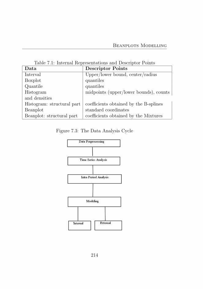
Beanplots Modelling
Table 7.1: Internal Representations and Descriptor PointsData Descriptor PointsInterval Upper/lower bound, center/radiusBoxplot quantilesQuantile quantilesHistogram midpoints (upper/lower bounds), countsand densitiesHistogram: structural part coefficients obtained by the B-splinesBeanplot standard coordinatesBeanplot: structural part coefficients obtained by the Mixtures
Figure 7.3: The Data Analysis Cycle
214
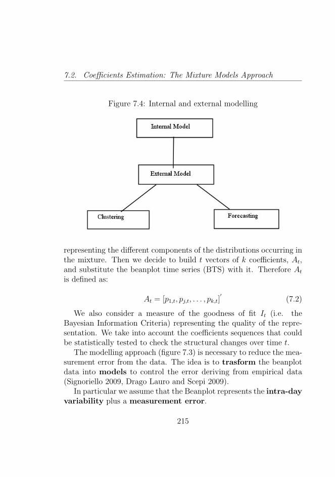
7.2. Coefficients Estimation: The Mixture Models Approach
Figure 7.4: Internal and external modelling
representing the different components of the distributions occurring inthe mixture. Then we decide to build t vectors of k coefficients, At,and substitute the beanplot time series (BTS) with it. Therefore Atis defined as:
At = [p1,t, pj,t, . . . , pk,t]′
(7.2)
We also consider a measure of the goodness of fit It (i.e. theBayesian Information Criteria) representing the quality of the repre-sentation. We take into account the coefficients sequences that couldbe statistically tested to check the structural changes over time t.
The modelling approach (figure 7.3) is necessary to reduce the mea-surement error from the data. The idea is to trasform the beanplotdata into models to control the error deriving from empirical data(Signoriello 2009, Drago Lauro and Scepi 2009).
In particular we assume that the Beanplot represents the intra-dayvariability plus a measurement error.
215
Beanplots Modelling
Beanplot Data = Model + Error (7.3)
By considering the visualization of the beanplot time series (BTS)we choose a kernel and a bandwidth. With the aim of modelling andforecasting beanplot time series (BTS), a coefficients estimationbecomes necessary.
We can assume each initial intra-day observation characterized inthis sense:
g(x) = p1f1(x) + · · ·+ pkfk(x) (7.4)
With 0 ≤ pi ≤ 1 and i = 1 . . . k and also p1 + p2 + · · · + pk = 1.So we have g() as a finite mixture density function. The coefficientsp1 . . . pk will be the model coefficients where the f1(.) . . . fk(.) are thecomponent densities of the mixture. So we have: fj(x) = f(x|θj)where θj defines the coefficients in fj(x).
By fixing the initial number of component densities of the mixtureN we have for the beanplot data:
g(x|Ψ) =k∑j=1
pjf(x|θj) + η (7.5)
where η is a specific associated error and Ψ = (p1 . . . pk, θ1, . . . , θk)′
are the complete list of coefficients of the mixture model.We fix both K and h and we derive the density model time series
as a mixture of different distributions.We retain the coefficients pj representing the different components
of the distributions occurring in the mixture.In particular, the estimation method used is the maximum likeli-
hood method, where it is necessary to consider some starting points(obtained by the beanplot analysis). A complete overview of themethod used is in Du 2002 [239].
216
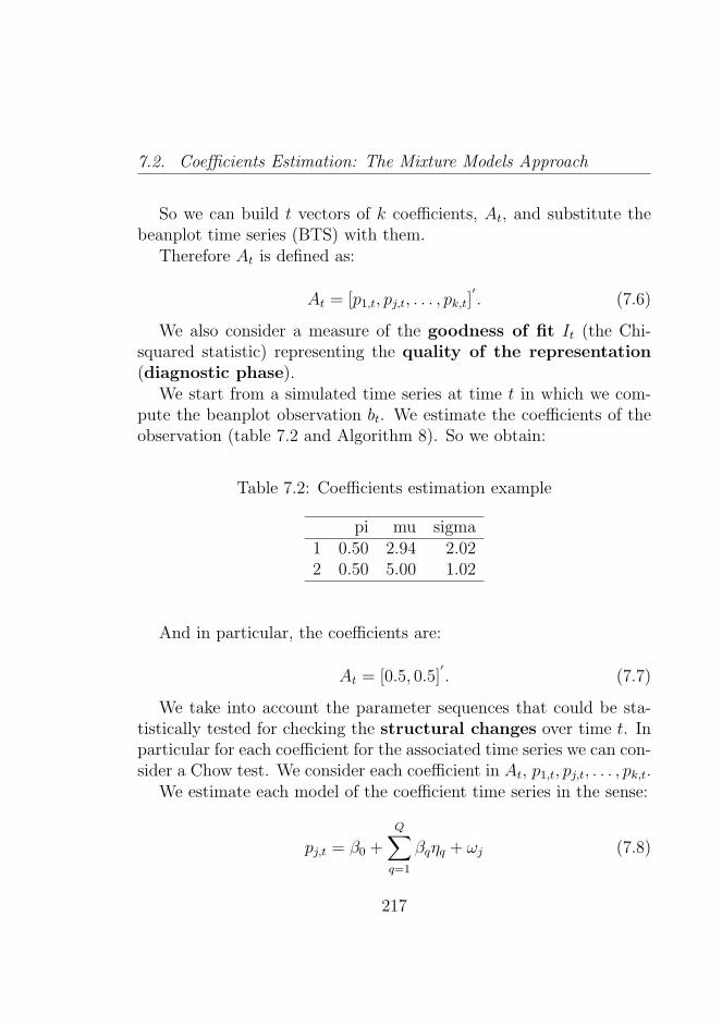
7.2. Coefficients Estimation: The Mixture Models Approach
So we can build t vectors of k coefficients, At, and substitute thebeanplot time series (BTS) with them.
Therefore At is defined as:
At = [p1,t, pj,t, . . . , pk,t]′. (7.6)
We also consider a measure of the goodness of fit It (the Chi-squared statistic) representing the quality of the representation(diagnostic phase).
We start from a simulated time series at time t in which we com-pute the beanplot observation bt. We estimate the coefficients of theobservation (table 7.2 and Algorithm 8). So we obtain:
Table 7.2: Coefficients estimation example
pi mu sigma1 0.50 2.94 2.022 0.50 5.00 1.02
And in particular, the coefficients are:
At = [0.5, 0.5]′. (7.7)
We take into account the parameter sequences that could be sta-tistically tested for checking the structural changes over time t. Inparticular for each coefficient for the associated time series we can con-sider a Chow test. We consider each coefficient in At, p1,t, pj,t, . . . , pk,t.
We estimate each model of the coefficient time series in the sense:
pj,t = β0 +
Q∑q=1
βqηq + ωj (7.8)
217
Beanplots Modelling
where ηq is a dummy variable (0, 1) that represents a specific periodor an interval period of time, in which the null hypothesis of no struc-tural change is tested. In the presence of structural change βq 6= 0. Atthe same time ωj is a residual. We return the dates of the structuralchanges for all the coefficients in At
Data: A Beanplot time series (BTS) bYt t = 1...TResult: A vector At with the p as the proportions of the
mixture components, given the bandwidth hbegin
Choice of the I temporal intervalChoice of the n pointsChoice of the h bandwidth to usefor t ∈ T do
Estimating the coefficients of the mixture model for theBeanplot Bt
endAre the internal models not fitting data adequately?if the internal model is not adequately fitted then
change the number of coefficients p or the intervaltemporal I
end
endAlgorithm 8: Beanplot internal modelling: coefficients estimation
7.2.1 Choosing the optimal interval temporal
It is necessary to consider as the optimal, the temporal interval relatedto the lowest error. In practice we compare different specifications overthe time and we decide on the best one by considering the index of
218
7.3. Beanplot Representations by their Descriptor Points
goodness of fit over the time. We decide this by combining the differentgoodness of fit (using for example, a mean of the different goodnessof fit) and we choose the interval temporal that minimizes this index.The algorithm is shown in algorithm 8 (page 220).
7.3 Beanplot Representations by their De-
scriptor Points
Here we can obtain and specifically represent the beanplot shape. Inparticular we assume that the original beanplot shape is constitutedby two parts: a structured one (defined as a ”model”) plus a residual(in this sense we follow the approach to histogram approximation inSignoriello (2008)):
Bt = Mt + Et(t = 1...T ) (7.9)
where B are the real data (the beanplot representations in the case)at temporal interval t, M represents the model, and E is the residualpart. We need to represent the structured part Mt and minimize theresidual part Et.
We know that for every probability density function φ(x), for anyprobability density function the area is represented by:∫ ∞
−∞φ(x)dx = 1 (7.10)
Or also:
fh,t =1
nh
i=1∑n
K(x− xih
) =
∫ ∞−∞
φ(x)dx = 1 (7.11)
219
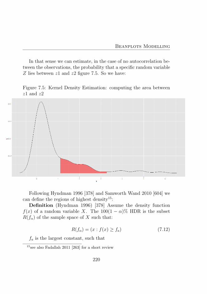
Beanplots Modelling
In that sense we can estimate, in the case of no autocorrelation be-tween the observations, the probability that a specific random variableZ lies between z1 and z2 figure 7.5. So we have:
Figure 7.5: Kernel Density Estimation: computing the area betweenz1 and z2
Following Hyndman 1996 [378] and Samworth Wand 2010 [604] wecan define the regions of highest density15:
Definition (Hyndman 1996) [378] Assume the density functionf(x) of a random variable X. The 100(1 − α)% HDR is the subsetR(fα) of the sample space of X such that:
R(fα) = (x : f(x) ≥ fa) (7.12)
fa is the largest constant, such that
15see also Fadallah 2011 [263] for a short review
220
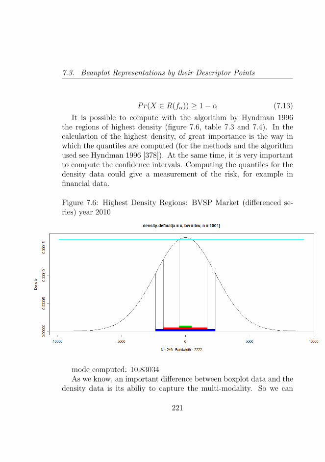
7.3. Beanplot Representations by their Descriptor Points
Pr(X ∈ R(fα)) ≥ 1− α (7.13)
It is possible to compute with the algorithm by Hyndman 1996the regions of highest density (figure 7.6, table 7.3 and 7.4). In thecalculation of the highest density, of great importance is the way inwhich the quantiles are computed (for the methods and the algorithmused see Hyndman 1996 [378]). At the same time, it is very importantto compute the confidence intervals. Computing the quantiles for thedensity data could give a measurement of the risk, for example infinancial data.
Figure 7.6: Highest Density Regions: BVSP Market (differenced se-ries) year 2010
mode computed: 10.83034As we know, an important difference between boxplot data and the
density data is its abiliy to capture the multi-modality. So we can
221
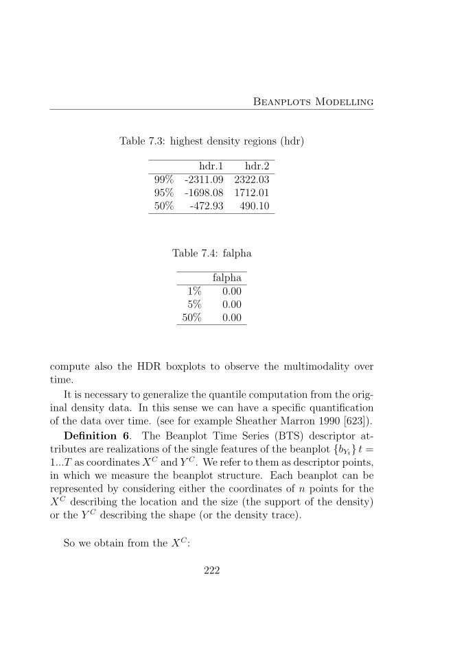
Beanplots Modelling
Table 7.3: highest density regions (hdr)
hdr.1 hdr.299% -2311.09 2322.0395% -1698.08 1712.0150% -472.93 490.10
Table 7.4: falpha
falpha1% 0.005% 0.00
50% 0.00
compute also the HDR boxplots to observe the multimodality overtime.
It is necessary to generalize the quantile computation from the orig-inal density data. In this sense we can have a specific quantificationof the data over time. (see for example Sheather Marron 1990 [623]).
Definition 6. The Beanplot Time Series (BTS) descriptor at-tributes are realizations of the single features of the beanplot bYt t =1...T as coordinatesXC and Y C . We refer to them as descriptor points,in which we measure the beanplot structure. Each beanplot can berepresented by considering either the coordinates of n points for theXC describing the location and the size (the support of the density)or the Y C describing the shape (or the density trace).
So we obtain from the XC :
222
7.3. Beanplot Representations by their Descriptor Points
XC = [x1,t, xj,t, . . . , xk,t]′
(7.14)
And from the Y C :
Y C = [y1,t, yj,t, . . . , xk,t]′
(7.15)
To specifically represent the beanplot we choose firstly the numbern of descriptor points to represent the initial density and then we ob-tain numerically the coordinates XC and Y C (Algorithm 9). The XC
represents the values in which the density Y C is calculated.
In particular the Y C value represents an estimate of the probabil-ity density at the point represented by XC value. If we consider ahigher number of points n in the procedure we obtain a more preciseapproximation of the original beanplot. In practice the choice of thenumber of points to describe the density corresponds to the choice ofthe number of bins in a histogram. However when we use a kernelestimation procedure we have higher flexibility than in the histogramcase to separate the structure and to decide the optimal number ofpoints. The choice of the descriptors n is a problem of finding theexact representation of the underlying phenomenon: are we interestedonly in a stylized image of the beanplot or do we need to representall the features of the beanplots? In general are we correctly repre-senting the underlying data? The different choices of the bandwidthand the kernel can improve the representation of the data, so when weobtain a satisfying data representation we can proceed to forecastingthe process (algorithm 1).
The choice of h can be constrained to a number of descriptor pointsn to compute. A higher h (computed by the Sheather-Jones Method)can be an indicator of structural change in the internal model, there-fore a coherent choice of the h needs to be made. By choosing a higher
223
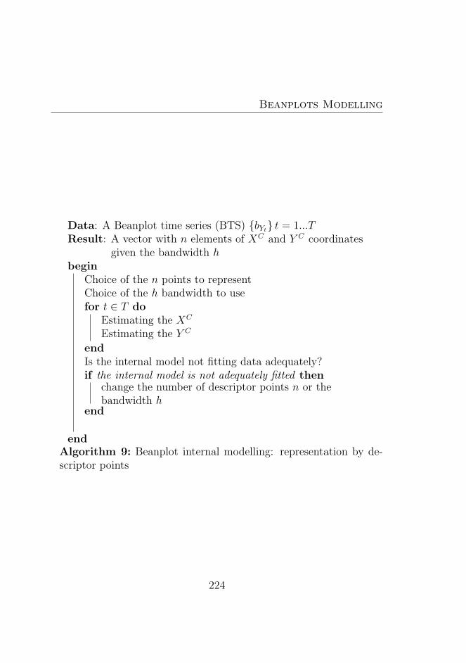
Beanplots Modelling
Data: A Beanplot time series (BTS) bYt t = 1...TResult: A vector with n elements of XC and Y C coordinates
given the bandwidth hbegin
Choice of the n points to representChoice of the h bandwidth to usefor t ∈ T do
Estimating the XC
Estimating the Y C
endIs the internal model not fitting data adequately?if the internal model is not adequately fitted then
change the number of descriptor points n or thebandwidth h
end
endAlgorithm 9: Beanplot internal modelling: representation by de-scriptor points
224
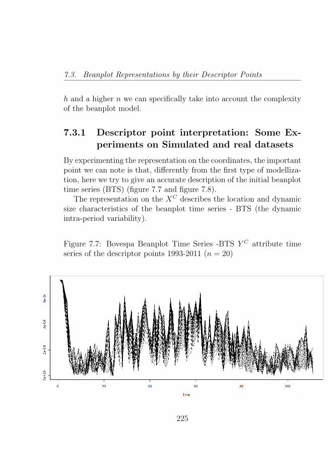
7.3. Beanplot Representations by their Descriptor Points
h and a higher n we can specifically take into account the complexityof the beanplot model.
7.3.1 Descriptor point interpretation: Some Ex-periments on Simulated and real datasets
By experimenting the representation on the coordinates, the importantpoint we can note is that, differently from the first type of modelliza-tion, here we try to give an accurate description of the initial beanplottime series (BTS) (figure 7.7 and figure 7.8).
The representation on the XC describes the location and dynamicsize characteristics of the beanplot time series - BTS (the dynamicintra-period variability).
Figure 7.7: Bovespa Beanplot Time Series -BTS Y C attribute timeseries of the descriptor points 1993-2011 (n = 20)
225
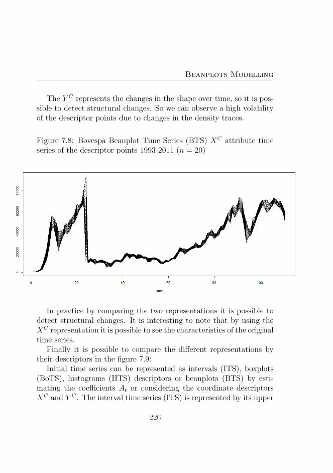
Beanplots Modelling
The Y C represents the changes in the shape over time, so it is pos-sible to detect structural changes. So we can observe a high volatilityof the descriptor points due to changes in the density traces.
Figure 7.8: Bovespa Beanplot Time Series (BTS) XC attribute timeseries of the descriptor points 1993-2011 (n = 20)
In practice by comparing the two representations it is possible todetect structural changes. It is interesting to note that by using theXC representation it is possible to see the characteristics of the originaltime series.
Finally it is possible to compare the different representations bytheir descriptors in the figure 7.9:
Initial time series can be represented as intervals (ITS), boxplots(BoTS), histograms (HTS) descriptors or beanplots (BTS) by esti-mating the coefficients At or considering the coordinate descriptorsXC and Y C . The interval time series (ITS) is represented by its upper
226
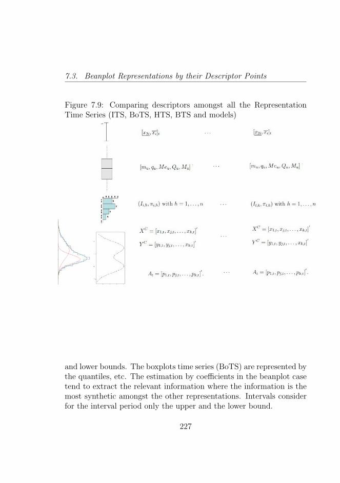
7.3. Beanplot Representations by their Descriptor Points
Figure 7.9: Comparing descriptors amongst all the RepresentationTime Series (ITS, BoTS, HTS, BTS and models)
and lower bounds. The boxplots time series (BoTS) are represented bythe quantiles, etc. The estimation by coefficients in the beanplot casetend to extract the relevant information where the information is themost synthetic amongst the other representations. Intervals considerfor the interval period only the upper and the lower bound.
227
Beanplots Modelling
7.4 Data Tables considering Density rep-
resentations
It is possible, now, to define what the coefficients and the descriptorpoints contribute in the generation of a specific data matrix that couldbe statistically analyzed.
In this respect, by starting from the classical time series we obtainthe symbolic time series and the symbolic time series data table ([211]and figure 7.10). It is important to note that handling different out-liers can be very important because we can obtain different results bytaking into account different symbolic data. In this specific case thesymbolic data analysis came directly from the data. Through choosingthe best statistical descriptor we analyse these series using symbolicdata analysis. See also Gettler-Summa M. Frederick V. (2010) [299].The objective of this thesis is to handle symbolic data which can bedensities.
Following Signoriello 2008 [630], the function considered (or thestatistical model in the wide sense) is substituted by the estimatedcoefficients and the descriptor points, so we obtain a final data tablewhich is useful for the statistical analysis of the intra-variation be-tween different models using the appropriate techniques.
In the data matrix of the estimated coefficients the data can beconsidered as units× variables× number of coefficients.
Each different function or model needs to be accompanied by thegoodness of fit, or its ability to fit the original data. So in each cell weneed to have k coefficients and an index (I) of goodness of fit. Fromthe models and their goodness of fit it is possible to obtain a summaryof the intra-period variation and the presence of models that are notwell approximated.
228
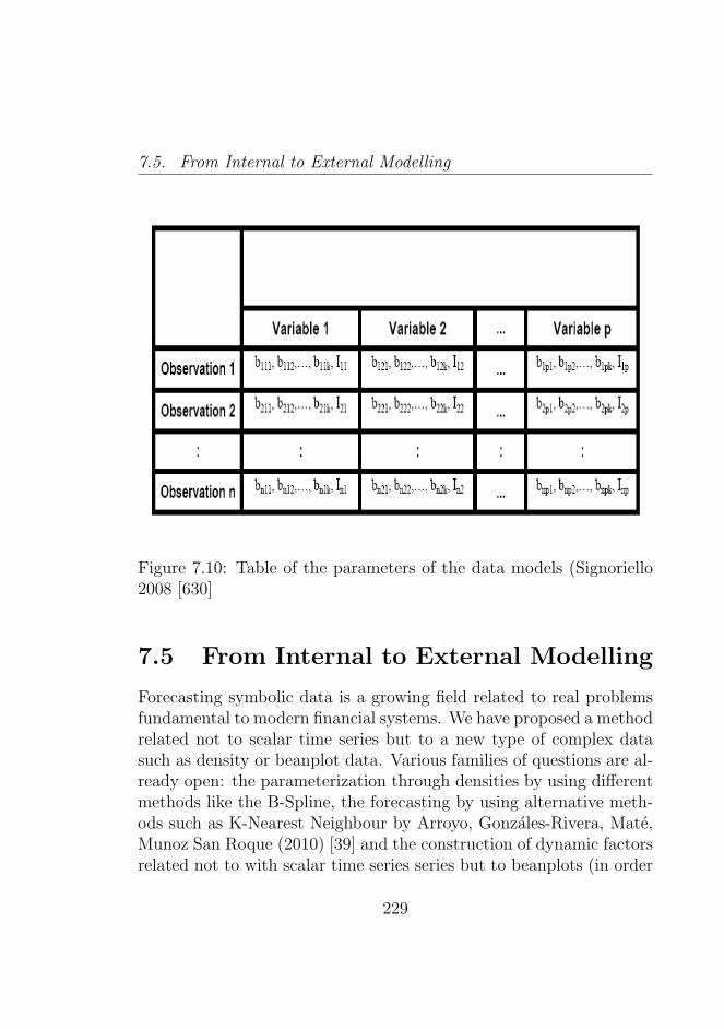
7.5. From Internal to External Modelling
Figure 7.10: Table of the parameters of the data models (Signoriello2008 [630]
7.5 From Internal to External Modelling
Forecasting symbolic data is a growing field related to real problemsfundamental to modern financial systems. We have proposed a methodrelated not to scalar time series but to a new type of complex datasuch as density or beanplot data. Various families of questions are al-ready open: the parameterization through densities by using differentmethods like the B-Spline, the forecasting by using alternative meth-ods such as K-Nearest Neighbour by Arroyo, Gonzales-Rivera, Mate,Munoz San Roque (2010) [39] and the construction of dynamic factorsrelated not to with scalar time series series but to beanplots (in order
229
Beanplots Modelling
to improve forecasting by using different beanplot time series BTS).We need at this point to compute a way to tell if the forecasts ob-
tained by the different models are good or not. So we build indicesto study the level of the adequacy of the forecasts obtained by thedifferent models.
7.5.1 Detecting Internal Models as Outliers
It is possible to use a clustering procedure to identify the outliers. Inpractice we use a distance (for example, the euclidean distance on thecoordinates and the model distance on the coefficients of the mixture)to identify the different models that could be considered outliers.
In this sense we can conclude that the elimination of the noise is notsuccessful and that we need to eliminate these extreme observations.
So we can proceed by either not considering the extreme observa-tions, or by imputating them. In fact, we need to analyze the externalmodels and either consider or not these extreme values (identified hereas outliers).
A second strategy starts from the estimated coefficients and thedescriptor points so as to identify from the trajectories the outliers(using a method that identifies outliers from the time series16). In thisrespect we identify outliers directly from external models.
7.6 Internal Models Simulation
From the Internal Models we can simulate the same internal models.This is useful for various reasons. In general we start from the primarydata and we try to simulate n times the data generating process ofthe complex data through obtaining the data characteristics than can
16For example see Chang, Tiao and Chen (1988) [130] and Riani 2004 [582]
230
7.6. Internal Models Simulation
mimic the initial data. If the difference is small that means that theNoise part is not relevant. The structural part in this sense could bedetected as a representation in the internal model as a density data.The aim of the simulation exercise is to simulate different scenariosand understand if the most important and relevant features of thedata are captured by the models.
In particular the important question is: are the models good foridentifying important data features of the reality, can we understandthe structural part of the initial data and separate it from the noise?
231
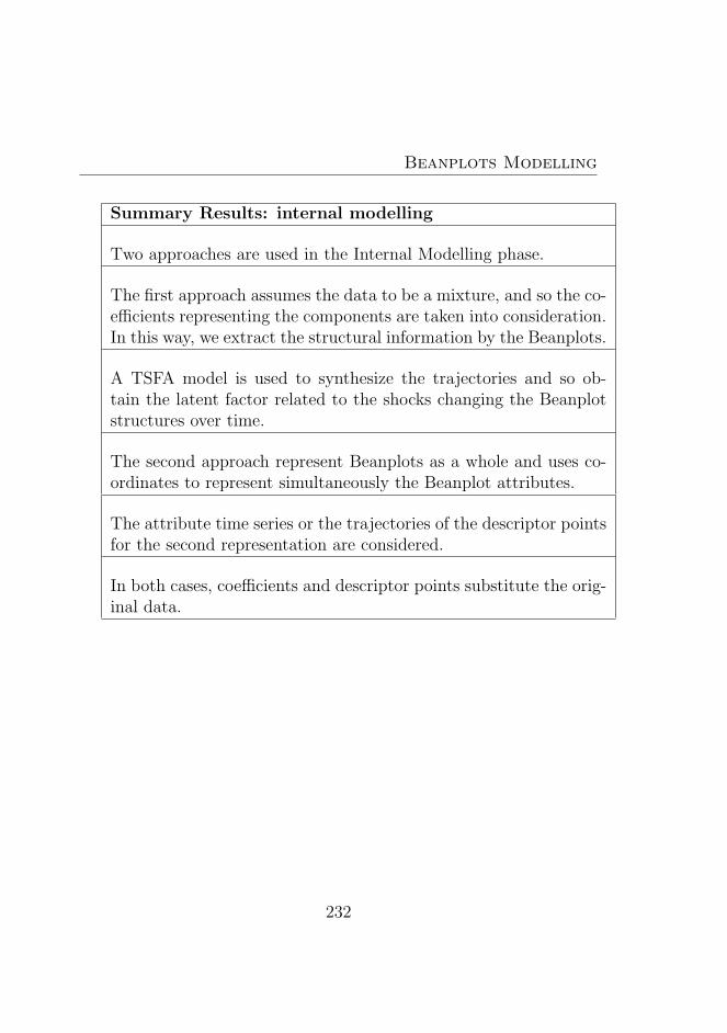
Beanplots Modelling
Summary Results: internal modelling
Two approaches are used in the Internal Modelling phase.
The first approach assumes the data to be a mixture, and so the co-efficients representing the components are taken into consideration.In this way, we extract the structural information by the Beanplots.
A TSFA model is used to synthesize the trajectories and so ob-tain the latent factor related to the shocks changing the Beanplotstructures over time.
The second approach represent Beanplots as a whole and uses co-ordinates to represent simultaneously the Beanplot attributes.
The attribute time series or the trajectories of the descriptor pointsfor the second representation are considered.
In both cases, coefficients and descriptor points substitute the orig-inal data.
232
Chapter 8
Beanplots Time SeriesForecasting
Scalar Time Series (STS) Analysis and Forecasting1 is the analysis ofthe characteristics of a time series and the application of a statisticalmodel to forecast its future values.
Very relevant research developments have occurred in this field andimportant results have been obtained since the 1970’s (De Gooijer andHyndman (2006) [180]). Forecasting of time series data2 is a difficulttask when the data are very numerous, with complex structure3 forexample, when there are high volatility and structural changes (for the
1Hamilton 1994 [333] Lutkepohl 2005 [469], Battaglia 2007 [66], Durbin Koop-man (2001) [244] and Elliott and Timmermann (2008) [247]. An important reviewwork on Forecasting is De Gooijer Hyndman (2006) [180]
2Box Jenkins 1976 [99] Wallis 1989 [767]3The financial markets for example are considered a complex system (in this
sense: Marschinski and Matassini 2001 [488], Mauboussin 2002 [496], Sornette2004 [636] and Tjung, Kwon, Tseng, Bradley-Geist (2010) [661]. Of relevanceis the difference between signal and noise provided by the same operators thatimpacts on price, see for example the experiment in Cipriani and Guarino 2005[144]
Beanplots Time Series Forecasting
problems and the approaches in forecasting financial data see DeistlerZinner 2007 [187]). This is the case of high frequency data or, ingeneral, of financial data, where we cannot clearly visualize the singledata4 and where the necessity of an aggregation arises (see Chapter 1and Chapter 2). A first proposal is that of using in addition to classicalscalar time series some ”density based” time series (see Chapter 5for the characteristics of the density data) and in particular beanplottime series (BTS). In this chapter we deal with the specific problem offorecasting the beanplot time series (BTS). So we propose an approachbased firstly on internal models (as we have seen in Chapter 7) of thebeanplot time series (BTS) and successively on the choice of the bestforecasting method with respect to our data. In particular we proposea strategy to use combination forecast methods5 in order to improvethe statistical performance of our forecasts.
8.1 Density Forecasting and Density Data
There are important differences between density forecasting6 and theforecasting of density data. Density forecasting can be defined as ”adensity forecast of the realization of a random variable at some futuretime is an estimate of the probability distribution of the possible futurevalues of that variable” (see Tay Wallis 2000 [653]). In the analysis ofthe density data we consider the densities for each temporal intervalas data, and we build external models on them.
In the analysis of complex time series, such as high frequency data
4Zivot (2005) [722]5See for a discussion of these methods Timmermann 2006 [658], Clemen (1989)
[145] Armstrong 2001 [29] who review the method. For a formal explanation onwhy forecast combinations of single forecasts tend to outperform sophisticatedmodels see Smith and Wallis 2009 [635]
6Timmermann 2000 [657] Bao Lee and Saltoglu 2007 [59] Diebold Gunther 1997[220]
234
8.1. Density Forecasting and Density Data
or financial data with a particular data structure, it is not alwayspossible to have an effective visualization and reliable forecasting. Inforecasting, the problem of the visualization and the choice of themodel to use are specifically linked, in fact, in identifying the ade-quate one it can be important to detect outliers. The problem of thevisualization of complex time series has been particularly explored in apaper proposed by Drago and Scepi in 2009 [237] where we underlinedthe necessity of searching and analysing an aggregate behaviour forcomplex data and we have explored aggregated beanplot time series(BTS) to observe their characteristics. In particular we have shownthe proprieties of beanplot time series (BTS) by comparing differenttypes of aggregated time series and by illustrating their statistical per-formances in financial data interpretation. In this chapter we proposean approach for forecasting beanplot time series (BTS). In particular,after a short introduction on the definition and the main characteris-tics of beanplot time series (BTS), we deal with the problem of findingan appropriate internal model to define an external model with the aimof forecasting beanplot time series (BTS). We propose our forecastingapproach in Sections 9.3 and 9.4 in a summarized form while we il-lustrate it in greater detail in the applicative section. We show thatthe advantage of our approach is to forecast not only the average orthe location of the data but at the same time to predict the size andthe shape of the data (the entire structure). In the specific case offinancial and high frequency data we are trying to genuinely predictthe associated risk or the volatility that can occur over time. Size andshape can represent the internal variation over the interval temporal,so, in this sense there is a specific link between the data collectionand quantitative methods used: we try to forecast the market insta-bility or the internal variation in the data. For density forecasting seeHyndman and Fan (2008) [387]. Tay Wallis (2000) [653]
235
Beanplots Time Series Forecasting
8.2 From Internal Modelling to Forecast-
ing
The Beanplot time series (BTS) bYt t = 1...T is an ordered sequenceof beanplots or densities over time (see Drago Scepi 2009 [237]). Thetime series values can be viewed as realizations of an X beanplotvariable in the temporal space T , where t represents the single timeinterval. For forecasting purposes the choice of the length of the singletime interval t (day, month, year) depends on the specific data featuresand objectives the analyst wants to study. In practice, detecting theadequate model means finding the outliers in the series before mov-ing on to the analysis, there is also the need to consider structuralchanges in the model. For this reason it is very important to considervisualization and clustering methods (in particular with the objectiveto detect outliers7 before proceeding to the analysis).
Various approaches could be considered:
1. Considering trajectories from the coefficients of the mixtures(Chapter 8.3)
2. Considering the trajectories from the beanplot descriptions orattribute time series (Chapter 8.4)
3. K-Neirest Neighbour (Chapter 8.5)
4. Forecast Combinations (Chapter 8.6)
5. Hybrid approaches (Chapter 8.6)
6. Uses of GA (Chapter 8.6)
7. Forecasting using the Search Algorithm (Chapter 8.7)
7In scalar data: see for example Cherednichenko 2005 [132]
236
8.3. External Modelling (I): TSFA from model coefficient approach
8.3 External Modelling (I): TSFA from
model coefficient approach
We start from an internal model described, like the coefficients of theextracted mixtures, in Chapter 4. In this sense we are considering thesequence of the coefficients over the time. The beanplots are entirelysubstituted by these coefficients sequences.
We can forecast the next beanplot at t + 1 by considering a timeseries forecasting method. Starting from the Time Series Factor Anal-ysis (in particular Meijer Gilbert 2005 [500]), in practice, we can defineeach vector of coefficients as a combination of time factors:
pt = α + V ξt + εt (8.1)
with α as a vector of intercepts, V as a J ×M matrix of factorloadings and εt as a vector of random errors. So, by considering Kobserved pj,t with j = 1..J and t = 1..T , in which we are searching theM factors as unobserved processes ξm,t with m = 1..M and t = 1..T .Therefore, for each time series we can obtain a number q ≤ k numberof factors. The loadings L are estimated by FA estimators (such asML), by using the sample covariance of the error (Wansbeek Meijer2005 [689])
To measure the factor, we use:
ξt = (V tΨt−1V )−1V tΨ−1V t(pt − αt) (8.2)
In which ψt = Cov(εt). In particular the loadings, in the FA esti-mators (say, ML), can be estimated by using the sample covariance ofthe error.
The usual assumption made in TSFA is that αt = 0, so the Bartlettpredictor becomes:
ξt = (V tΨt−1V )−1V tΨ−1V t(pt). (8.3)
237
Beanplots Time Series Forecasting
In this way, it is possible to compute the factor time series forthe factors related to the location and the size and another factorrepresenting the shock response or the short run dynamics. We can usedifferent forecasting methods for forecasting the different time factors(starting from an ARMA model). In particular, for forecasting factortime series using the TSFA see Munoz , Corchero and Javier Heredia(2009) [523]:
ξt = c+ wt +r∑s=1
ϕsξt−s +
q∑s=1
θswt−s. (8.4)
Starting from the prediction of the factors, from eq. (4) we cancompute the initial coefficients by giving the value of the ξt. So wehave:
pt = α + V ξt + εt (8.5)
From the predictions of the initial coefficients we can fit the pre-dicted beanplots. Assuming the number of initial groups of mixturesNj=1...k we have for the beanplot:
Bt =k∑j=1
pj,tNj,t + ηt (8.6)
Where ηt is a specific associated error.
From the predictions of the coefficients we can fit the observedbeanplots Bt. Poor results in in-sample forecasting can occur in arevision of the initial parameters considered (the kernel K used andthe bandwidth h for example). At the same time, poor forecastingresults can be useful in order to identify structural changes, outliersor abnormal influent observations.
238
8.3. External Modelling (I): TSFA from model coefficient approach
We use the combination of the forecasts to improve the forecasts inthe presence of model parameter drifts and uncertainty in the identi-fication procedure
FCMt = γ1(t)f 1
t + γ2(t)f 2t + · · ·+ γm(t)fmt (8.7)
In the combination of the forecasts we use f1 . . . fm forecasting tech-niques (i.e Exponential Smoothing8, Splinef9, Theta methods10). Var-ious strategies of the weight estimation of the combination modelγ1 . . . γm are used. By considering explicitly f 1, f 2 . . . fm as differ-ent forecasts from competing external models we have as externalmodel the forecast combination Ft. In this case γ1 . . . γn are differ-ent weights. In particular the weighted combination11 of the modelsallows one to improve forecasting in a context of parameter drift andstructural change.
Poor results in in-sample forecasting can occur in a revision of theinitial parameters considered (the kernel K used and the bandwidthh for example), in order to identify outliers or abnormal influent ob-servations. A search algorithm is used in the validation phases toimprove the predictions by selecting the best relevant information asforecasting interval.
8Hyndman, Koehler, Snyder and Grose (2002)[384] Hyndman, Koehler, Ordand Snyder (2008) [385] Hyndman, Akram, and Archibald (2008) [380]
9 Hyndman, King, Pitrun and Billah (2005) [388]10 Assimakopoulos and Nikolopoulos (2000) [45], Hyndman and Billah (2003)
[381], Makridakis Wheelwright Hyndman (2008) [480]11Winkler Makridakis 1983 [703] Bates Granger 1969 [64] Newbold Granger 1974
[534]
239
Beanplots Time Series Forecasting
8.3.1 Detecting Structural Changes
Coefficient sequences could be statistically tested for checking thestructural changes over time t. We use a different Chow test12
in every associated time series for each coefficient.We consider each coefficient in At, p1,t, pj,t, . . . , pk,t. We estimate
each model of estimated coefficients time series in this sense:
pj,t = β0 +
Q∑q=1
βqδq + ωj (8.8)
where δq is a dummy variable (0, 1) that is representing a specificperiod or an interval period of time, in which the null hypothesis ofno structural change is tested. In the presence of structural changeβq 6= 0. At the same time ωj is a residual.
We return the dates of the structural changes for all the coefficientsto At
8.3.2 Examples on real data: Forecasting WorldMarket Indices
This application has twofold objectives. The application is dividedinto two parts: We consider firstly the time series of the Dow JonesIndex for the period 1990-2010 and we compare three different ap-proaches in forecasting: scalar data, beanplots and interval valuedtime series. Secondly, we study the mechanisms of the financial con-tagion between the financial systems in the crisis by trying to forecastother world indexes.
We consider the case of various markets and the beanplot time se-ries (BTS) related to the closing price. In practice, we examine variousmarket indexes in which we consider the high, low, close, and open
12Chow 1960 [140] Harvey 1990 [343] Chu Stinchcombe White 1996 [142]
240
8.3. External Modelling (I): TSFA from model coefficient approach
price for various periods (depending on the data availability of eachsingle market in Yahoo). For each dataset we consider the closing priceand we obtain the beanplot time series (BTS) for the single market aswell.
Then we model the beanplot by considering the beanplot as a mix-ture, and we obtain the sequence of the estimated coefficients overtime. At this point we can consider a factorial strategy (Time SeriesFactor Analysis or TSFA) so as to obtain the factor time series repre-senting the single market.
Then we can use a forecasting method, for example an ARIMA,to predict the market dynamics over time as represented in the factorconsidered (figure 8.1, figure 7.1, figure 7.1, figure 8.4, figure 8.5, figure8.6)
It is interesting to compare the results with interval data for thecase of the Dow Jones Index (DJI):
1. The scalar data does not allow us to forecast the internal vari-ation in the year (useful for risk management purposes).
2. Interval time series (ITS) does not permit us to observe in theperiod the intra period structural changes. The beanplotbumps allow us to observe the internal variation also in thissense.
3. The intra period seasonality aspect is not represented byaggregating the time series (using a mean) or in interval timeseries (ITS). The different mixtures can be interpreted in somecases as structures related to intra period seasonality.
241
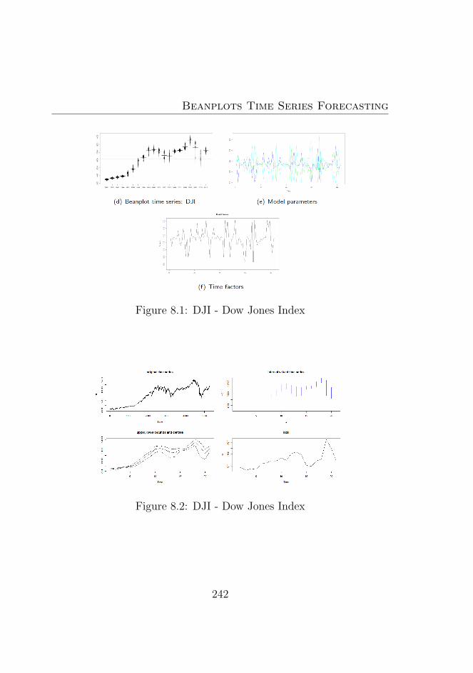
Beanplots Time Series Forecasting
Figure 8.1: DJI - Dow Jones Index
Figure 8.2: DJI - Dow Jones Index
242
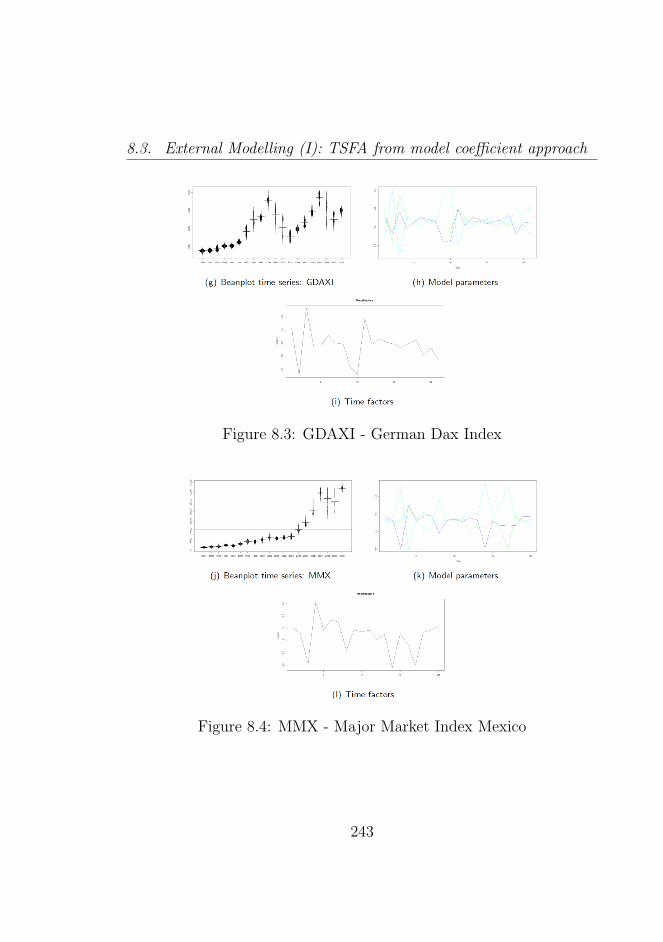
8.3. External Modelling (I): TSFA from model coefficient approach
Figure 8.3: GDAXI - German Dax Index
Figure 8.4: MMX - Major Market Index Mexico
243
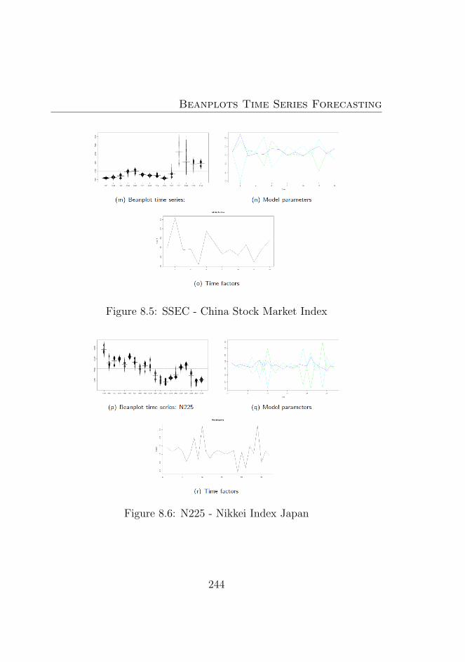
Beanplots Time Series Forecasting
Figure 8.5: SSEC - China Stock Market Index
Figure 8.6: N225 - Nikkei Index Japan
244
8.4. External Modelling (II): Attribute Time Series Approach fromCoordinates
8.4 External Modelling (II): Attribute Time
Series Approach from Coordinates
The second forecasting method is related to the approach of the co-ordinates. We need to define an internal model before forecasting.The idea is to represent each beanplot by using specific attributes ofeach beanplot and by considering their realization over the time. Sowe define a Beanplot Attribute Time Series as a realization of a sin-gle beanplot bYt t = 1...T descriptor over the time. To representthe beanplot time series (BTS) it is possible to consider the coordi-nates XC and Y C as descriptors of the beanplot. We refer to themas descriptor points because they measure the beanplot structure. Inparticular, the XC time series clearly show the location and the sizeof the beanplot over the time while the Y C represents well the shapeover the time. To specifically represent the beanplot we choose firstlythe number n of descriptor points and then we obtain numerically thecoordinates XC and Y C . If we consider a high number of points n inthe procedure we obtain a more precise approximation of the beanplot,here it is necessary to note that to have a density we have to considerat least 4 points (but not in every situation: we could be interested inforecasting the entire density trace).
The choice of the descriptors n is a problem of the exact modeliza-tion of the underlying phenomenon: are we interested only in a stylizedimage of the beanplot or do we need to represent all the features ofthe beanplots?
In our approach we consider the values of XC and Y C correspond-ing to the 25th, 50th and 75th percentile. The procedure is coherentwith existent literature (Arroyo 2009 [32]) in which, from the initialinterval data, the author obtains the attribute time series for the up-per and the lower bound. By this type of descriptor points we are ableto detect the evolution over the time of the beanplots, for the location,
245
Beanplots Time Series Forecasting
the size (both the XC) and the shape (mainly the Y C).
8.4.1 Analysis of the Attribute Time Series Ap-proaches
Our approach can be synthetized in the following steps. The first stepis the analysis of the structure of the sequence of the attributes. Inthis sense we have to test the structure of each attribute time series.As we know, they represent the beanplot dynamics over the time, sowe can use a specific method to forecast the attribute time series toobtain the prediction at time t + 1, t + 2 and so on. Initially we candetect the underlying structure of the data by decomposing the at-tribute time series. This decomposition can be very useful both tounderstand the general dynamics of the series over time (representedfor example by the trend) and to exploit some interesting patterns.
Successively we must decide which model has to be used for theforecasting approach. We can use univariate or multivariate meth-ods. In the first case we are assuming there is no specific relationshipbetween the attribute time series, in the second case we are assum-ing that a relationship exists (in practice we analyze attribute timeseries using time series analysis). So, it is firstly important to testthe stationarity of the attribute time series and successively to de-fine the possible cointegration between the series. Another importantpoint is to verify the autocorrelation of the attribute time series andthe possible structural changes. Only at the end of this first complexanalysis can we decide which model should be used for forecastingour attribute time series. After the identification of the forecastingmodels, it is necessary to estimate the different models for obtainingthe forecasts and, finally, to evaluate the reliability of our forecasts.The diagnostic procedure is very important because we can criticallyevaluate and respecify the models. At the same time it is very useful
246
8.4. External Modelling (II): Attribute Time Series Approach fromCoordinates
to consider the performances of the different forecasting models byconsidering some evaluation indexes. Using more than one forecastmay be necessary to obtain better predictions (see Timmermann 2006[658]).
So in general, an approach of forecast combinations may be neces-sary for many reasons. First of all there can be some structural changesand it may be necessary to take into account more than one forecast-ing model. In this sense, the use of different models can reduce therisk associated to choosing one single model. Secondly, there can besome uncertainty in the model to use, so it is very important to definea combination of forecast strategies to define the best model. Variousapproaches can be followed in setting the combination method. Onestrategy is to consider many different forecasts from several modelsand to use an average of them. Here, a relevant problem is the choiceof the different weights to apply on the different forecasting methods.Assigning higher weights to methods that permit the improvement ofthe accuracy of the forecasts (by minimizing errors) can be a solution.Finally, a relevant point could be the choice of the optimal interval forthe forecasting process.
8.4.2 Attribute Time Series Forecasting Models
Here we start to test the attribute time series. In particular we per-form the usual tests on nonstationarity for either the Y C and the XC
attribute time series on different subperiods. At the same time wedecompose the attribute time series to find some patterns that couldbe useful in the modelling phase. It is very interesting to note thatthe beanplots quickly change their features over the time, in partic-ular the shape, represented in the Y C attribute time series. So, forthe modelling purposes of the attribute time series we consider thelongest interval, and we test nonstationarity. We obtain the resultthat both the XC and the Y C attribute time series are nonstationary.
247
Beanplots Time Series Forecasting
Furthermore we perform the Cointegration Analysis, considering theattribute time series on the XC and those on the Y C . The final aim ofthis part is to investigate if in the case of the XC or in the Y C we canuse a Vector Error Correction Model in forecasting (see also Arroyo2009 [32] for an approach based on interval time series - ITS). To takein to specific account the structure of the single attribute time series,we identify various different models as starting forecasting models. Atthis point we estimate the different models also by considering thedifferent subperiods for robustness checking. The different forecastingmodels are evaluated in terms of different indexes of Forecasts Accu-racy13(see Hyndman Koehler 2006 [386]). At the same time if we canpredict the density data at the end we need to check if the integral ofthe area under the prediction is equal to 1. In this case the predictionof a density could be considered.
8.4.3 Identification and External Modelling Strat-egy
So we can summarize in this way the entire forecasting procedureusing the coordinate descriptor points in this way (Algorithm 10 andAlgorithm 11):
1. Start to consider the n attribute time series of the descriptors(i.e.x1,t, x2,t, x3,t, y1,t, y2,t, y3,t) of the beanplot time series (BTS)bYt for t = 1, ..., T
2. The attribute time series represent the external models (the dy-namics over the time t = 1, ..., T ) where each beanplot can beconsidered as the internal model at time t
13See also Armstrong 2006 [28]
248
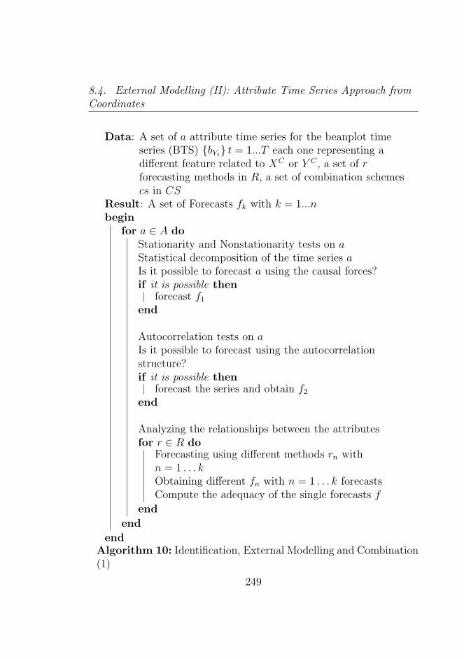
8.4. External Modelling (II): Attribute Time Series Approach fromCoordinates
Data: A set of a attribute time series for the beanplot timeseries (BTS) bYt t = 1...T each one representing adifferent feature related to XC or Y C , a set of rforecasting methods in R, a set of combination schemescs in CS
Result: A set of Forecasts fk with k = 1...nbegin
for a ∈ A doStationarity and Nonstationarity tests on aStatistical decomposition of the time series aIs it possible to forecast a using the causal forces?if it is possible then
forecast f1
end
Autocorrelation tests on aIs it possible to forecast using the autocorrelationstructure?if it is possible then
forecast the series and obtain f2
end
Analyzing the relationships between the attributesfor r ∈ R do
Forecasting using different methods rn withn = 1 . . . kObtaining different fn with n = 1 . . . k forecastsCompute the adequacy of the single forecasts f
end
end
endAlgorithm 10: Identification, External Modelling and Combination(1)
249
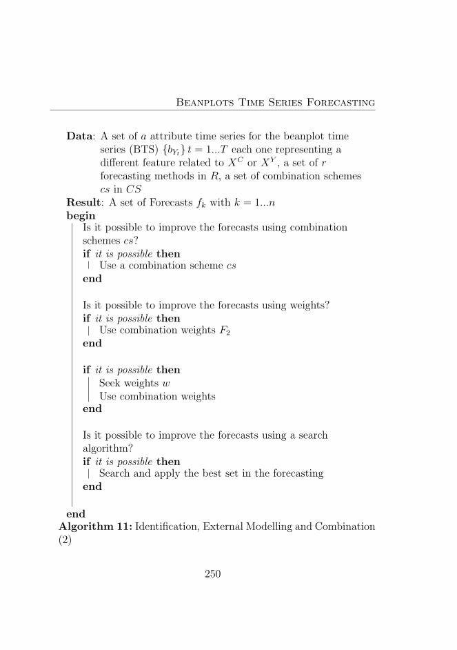
Beanplots Time Series Forecasting
Data: A set of a attribute time series for the beanplot timeseries (BTS) bYt t = 1...T each one representing adifferent feature related to XC or XY , a set of rforecasting methods in R, a set of combination schemescs in CS
Result: A set of Forecasts fk with k = 1...nbegin
Is it possible to improve the forecasts using combinationschemes cs?if it is possible then
Use a combination scheme csend
Is it possible to improve the forecasts using weights?if it is possible then
Use combination weights F2
end
if it is possible thenSeek weights wUse combination weights
end
Is it possible to improve the forecasts using a searchalgorithm?if it is possible then
Search and apply the best set in the forecastingend
endAlgorithm 11: Identification, External Modelling and Combination(2)
250
8.4. External Modelling (II): Attribute Time Series Approach fromCoordinates
3. Start to consider the n attribute time series of the descriptorsof the beanplot. They represent the beanplot dynamics over thetime
4. Checking for the stationarity and the autocorrelation. Detect-ing the features of the dynamics (trends, cycles, seasonality).Analyzing the relationships between the attributes
5. Forecasting using different methods
6. Beanplot Forecasts combinations schemes
7. Search Algorithm to improve forecasts
8. Considering as Beanplot description the forecasts obtained fromthe Forecasting Method.
9. Checking if the area of the predicted descriptor points can be adensity (the integral is equal to 1).
8.4.4 Examples on real data: Forecasting the Bean-plot Time Series (BTS) related to the DowJones Market
The application is related on the Dow Jones market dataset from theyear 1928 to the 2010, and the purpose is to forecast the beanplottime series (BTS) for the specific period 2009-2010. In particular weconsider in the models the data from 1998 to the 2008. The entireperiod in the database (1928-2010) is considered only for exploratorypurposes. The specific aim in the forecasting process is to predict theinstability in the market over the time. Methods used in the forecast-ing models are Smoothing Splines14 and Automatic Arima15 primarily,
14 Hyndman, King, Pitrun and Billah (2005) [388]15Hyndman and Khandakar 2008 [382]
251
Beanplots Time Series Forecasting
and also VAR16 (Vector Autoregressive Models) and VECM17 (VectorError Correction Models) in the case of the Y C attribute time seriesin some specific periods to analyse the robustness of the models (wework on different sub-periods to analyse the existence of structuralchanges in the period). In a second forecasting model we use a combi-nation approach, by combining different forecasts obtained by differentmethods. Lastly, we compare all the results, using as a benchmark:the Naive model (that is, representing the prediction obtained by con-sidering the last observation).
So as a first step in the procedure we visualize the entire beanplottime series (BTS) by considering the yearly temporal interval (wherethis interval is the most appropriate in the data exploration). We canclearly visualize the existence of the two crises, in particular the crisisin 2008, where we can observe the very peculiar shape of the beanplot,in that it is strongly stretched out. The rise and the fall of the NewEconomy in 2001 is visible as well in the data. At the same time it ispossible to detect the trends and the cycles of the beanplot time series(BTS) where we can also understand the structural change occurringover the time (for example in 2008).
We compute the set of XC attribute time series (year 1996-2010),starting from the representation by coordinates. Here we can considera different interval temporal from the interval used in the data visual-ization (that for considering the statistical features of the beanplots).At the end of the internal modelling process we obtain 6 attributetime series (3 for the XC and 3 for the Y C) and around 60 observa-tions (years 1996-2010 approximately).
The three XC attribute time series are related to the 25th, 50thand the 75th percentile where each Y C is associated to the XC . Wecall these intervals ”extreme risk intervals”, with minima or lower risk,
16 Lutkepohl H. (2005) [469] and Hamilton (1994) [333]17Lutkepohl H. (2005) [469]
252
8.5. The K-Neirest Neighbour method
median risk and maxima or upper risk. These intervals are directlyrelated to the beanplot structure. The attribute time series for the XC
show the long run dynamics of the beanplots and also the impact ofthe financial crisis. By considering the Y C attribute time series (year1996-2010), we need to remember that we are examining a differentinterval temporal (not the yearly interval temporal) but two months(around 40 observations in a beanplot data). In this representation wecan observe the complexity of the initial series, observed in particularin the changes time by time of the beanplot shapes (represented bythe Y C). These behaviors are related to the short run dynamics ofthe series. Now we can begin to test the stationarity for the attributetime series.
8.5 The K-Neirest Neighbour method
Here we can consider a method based on the K-Neirest Neighbouralgorithm. In particular we depart from a data matrix of the singleestimated coefficients or the descriptor points, and we forecast thedifferent beanplots in order to maximize the similarity of the periodsover time and consider a median of the values in time.Following Arroyo 2008 [32] and Arroyo, Gonzalez-Rivera, Mate (2010)[41] it is possible to use the K-Neirest Neighbour to predict the minimaand the maxima of the descriptor points of the beanplot. In practicewe follow two separate steps:
1. We search for the n interval sequences that could be defined asclosest to the current one.
2. The sequence extracted is necessary to consider this sequence ascharacterized by the last d intervals (the previous one).
253
Beanplots Time Series Forecasting
3. Clearly it is necessary to consider a distance to measure the dis-similarity of interval sequences regarding appropriate distances(see Arroyo 2008 [32])
4. We consider the mean of the subsequent interval of the n closestsequences to obtain the forecast.
5. Arroyo 2008 [32] proposes the use in the mean computation ofthe interval arithmetic (see in that sense Moore 1966 [513], Gioiaand Lauro 2005 [310] and Gioia 2001 [307])
6. Different weighting schemes can be applied
At the same time it is possible to consider the forecasts obtainedas a first forecast in a more complex combination of forecasts. So itis possible to consider the predictions obtained using the K-NeirestNeighbour as one of the weighted components in the forecast combi-nations (see in the context of interval data Salish and Rodrigues 2010[603]).
At the same time it is possible to use an approach on the entirebeanplot considering each different attribute time series separately(see Yakowitz 1987 [709] for the approach of K-Neirest Neighbour intime series analysis).
8.6 The Forecasts Combination Approach
Furthermore we use a different approach based on the ForecastingCombinations. In particular, we use combinations for two reasons: wecan take into account precisely the uncertainty in choosing a specificmodel (in fact sometimes the choice of a specification in a single fore-casting model can be very hard) and we can also take into accountthe specific structural changes that could be captured (or we try to
254
8.6. The Forecasts Combination Approach
capture) by considering combinations of forecasts. So we consider pre-dictions obtained by using various methods: Smoothing Splines, AutoArima, the mean of the period, the Theta method and the Exponen-tial Smoothing. See table 1 to compare the different MAPE for theXC .
We do not use any special weighting structure but we consideronly the average between results obtained from the different methods.Regarding the results, the forecasting performances outperform othersingle models based on the single forecasting model chosen. Here weare considering an interval of prediction of 5 periods ahead (for thisreason we do not apply this method to the Y C).
The forecast combinations are considered only on the XC forecast-ing because it was identified that their use allows us to obtain thebest specific predictions. The methods used in the combination pro-cedure are: Smoothing Splines, Auto Arima, the mean of the period,the Theta method and the Exponential Smoothing. In this way thesedifferent methods return forecasts, and the combined forecasts can beconsidered as the average of the models. As a prediction interval weuse an interval of 5 periods. It is interesting to note that the com-bination approach does not produce better results in every case incomparison with one method (the best one). At the same time as thepredictions from the forecasts in the XC and Y C attribute time serieswe can expect to capture the evolutionary features of the beanplots.It is clear that the predictions can have relevant consequences also forthe associated risk analysis (an increasing difference between beanplotextremes that can indicate a higher risk).
8.6.1 Combination Schemes
Various schemes of combination in forecasting can be used:
255
Beanplots Time Series Forecasting
1. Equal weighting (average) on the different methods SETAR18,KNN19, Regime Switching20, etc.
2. Different weighting proportional to the quality of the forecasts21
3. Different weighting considering a regression approach (a GrangerRamanathan Approach: see Granger Ramanathan 1984 [322] ).In this case it could be useful to consider different regressions likethe Nonlinear Least Squares NLS22 or the genetic algorithms23
4. Hybrid approaches to determine optimal decomposition of theseries and use them in a combination24
5. Ranking of the different forecasts25.
Following Timmermann 2006 [658] and Andrawis Atiya El-Shishiny2010 [18] let f be a forecast of a single so in all cases we have a set ofn forecast f at an interval t so we can combine.f is a forecast of a single model:
FCMt = w1(t)f 1
1 + w2(t)f 22 + w3f
33 + · · ·+ wmf
mt (8.9)
With: w1+w2+w3+...+wn = 1 and w(1) ≥ 0, w(2) ≥ 0...w(n) ≥ 0for all the weights w.
1. Base scenario: w1 = w2 = ....wn = 0 considering all forecasts
18Tong 1990 [665] Tong 1983 [664] Tong Lim 1980 [663]19Yakowitz 1987 [709]20Hamilton 2005 [334]21Timmermann 2006 [658] Andrawis Atiya El-Shishiny 2010 [18]22Fox 2002 [272]23Rousseeuw and van Driessen (2006) [598]24Zhang 2003 [717] and Maia, De Carvalho and Lurdermir 2006 [477]25Kisimbay 2010 [425]
256
8.6. The Forecasts Combination Approach
2. Alternative: w1...wn = 0 discarding some forecasts f1...fn, usingthe trimmed mean
3. Alternative: ft+h =√f 1t+h + f 2
t+h + ...fnt+h, using the geometric
mean. See Andrawis Atiya Shishiny (2010) [18] and Timmer-mann (2006) [658].
4. Alternative: using the harmonic mean: ft+h =nf1
t+hf2t+h...f
nt+h
f1t+h+f2
t+h+fnt+h
5. Weight determination: w1...wn ≥ 0, with: w1+w2+w3+...+wn =1
8.6.2 Optimal weight determination
At the same time the weights of the combination can be differentlydefined26:
1. w1 = w2 = ....wn = 0 as simple criteria has the advantage ofsimplicity, but clearly different alternatives could be chosen. Asecond approach can be related to the variance (we report herethe case of two weights as an example):
2. ft+h = [f 1t+h]
w1 + [f 1t+h]
w2 + ... + [fnt+h]1−w1+w2 optimal schemes
using a search algorithm using the geometric mean
3. Let two variances σ12 and σ2
2 σ12 represent the covariance betweenthe two forecasts. In this case, assuming the weight sum is 1
each weight can be obtained by: w1 =σ2
2−σ12
σ21+σ22−2σ12and also
w2 = 1− w1
26Timmermann 2006 [658] Andrawis Atiya El-Shishiny 2010 [18] Kang (1986)[417] Deutsch Granger Terasvirta 1994 [196]
257
Beanplots Time Series Forecasting
4. or also weighting by MSE (Stock Watson 2004 [644] ), so we
obtain: wh1 =∑k
j=−k MSE2h+j∑k
j=−k MSE1h+j+
∑kj=−k MSE2
h+j
and also
wh2 =∑k
j=−k MSE1h+j∑k
j=−k MSE2h+j+
∑kj=−k MSE1
h+j
8.6.3 Weight determination by regression
Another possibility is to directly estimate the weights by regression,having the different forecasts as independent variables and the truevalues as dependent.
In this case it is also possible to define various options at the sametime:
1. Linear weight parameterization: Granger and Ramanathan Com-bination27 estimate omitting the intercept: yt = β0f1 + β1f2 +...+ βnfn + εt
2. Nonlinear weights parameterization
3. Changing weights over the time28
8.6.4 Identification of the components to model
At the same time it is important to identify the eventual componentsof the models.
1. Assumption that the series is composed of parts: for exampleyt = Lt + Nt where Lt is a linear autocorrelation structure andNt is a non-linear component.
27Granger Ramanathan (1984) [322]28Deutsch, Granger, Terasvirta 1994 [196]
258
8.6. The Forecasts Combination Approach
2. Number of components to decompose the series29
3. Identification of the structured parts to decompose the series30.
8.6.5 Identification and implementation of the Hy-brid modelling strategy
At the same time it is possible to differently identify and implementthe models by considering a hybrid modelling strategy:
1. Methods choice, for example ARIMA, as in the case of Maia,De Carvalho, Ludermir (2006) [477] to estimate Lt then obtainεt = yt− Lt and use other methods, for example neural networksto capture the nonlinear structures of the yt. In particular εt =φ(εt−1, εt−2...εt−3) + kt. The single forecast fn from the model is:yt = Lt + Nt
2. Diagnostics
3. Combination Strategy. Combine f1,f2 etc.
Combinations using different assumptions
1. Different Hybrid Methods f1,f2 can be used, based on differentassumptions or hypotheses (interval data)
2. Combination strategy. Combine f1,f2 and so on.
29Hendry Hubrich 2006 [355] and Hendry Hubrich (2010) [356]30Hendry Hubrich 2006 [355] and Hendry Hubrich (2010) [356]
259
Beanplots Time Series Forecasting
8.6.6 Using Neural Networks and Genetic Algo-rithm in the modelling process
Neural Networks31, were used in literature to improve the forecast-ing process of interval data (in particular see Munoz, Mate, Arroyo,Sarabia (2007) [522] Garcıa Ascanioand Mate 2010 [291] and Mateand Garcıa Ascanio 2010 [494]). At the same time there are manystudies that use neural networks in stock forecasting (see for exampleLawrence 1997 [451] and Weckman et al 2008 [695])
So an option can be to use this approach in the forecasting of theattribute time series. In this work, in particular as a learning scheme,the Multilayer Perceptron was used to forecast some attribute timeseries (mainly the Y C) that present a sinusoidal trajectory. The pro-cedure was useful in analysing attribute time series which show thesecharacteristics.
The genetic algorithm can be used in two different contexts in orderto optimize predictions both as single forecast, or in forecast combi-nation schemes.
First of all we can use the genetic algorithm to explore the bestmodels we can define where it could be particularly difficult to modelthe data (for example in the case of the Y C coordinates of the bean-plot data). In that sense the Genetic Algorithm can help to identifythe model using a Symbolic Regression (for the entire procedure seeSchmidt Lipson in various works, for example: [608] , [610], [612] and[614]). However it should be stressed that this process is very usefulin conditions of attribute time series characterized by relevant noise.
Secondly we can use the genetic algorithms to optimize the modelsin the case of forecasts combinations. We can consider the geneticalgorithms in the regression to estimate the parameters of the combi-
31The literature in this area is enormous. An introduction can be found inWitten Frank 1999 [704] and Fabbri Orsini (1993) [258]
260
8.7. The Search Algorithm
nation model, avoiding the effects due to outliers or a strange value.In this respect the results obtained can be more robust, whilst the
robustification of the procedure can improve the final forecasts (seeWildi 2007 [700]).
8.7 The Search Algorithm
There is a growing literature on finding the adequate estimation win-dow: see Pesaran Timmermann 2007 [559] and Pesaran Pick 2010[557]. The search algorithm is useful in detecting the best informa-tion set for the prediction. So the forecast processes are repeated toconsider all the possible sets of information, where the model min-imizing some statistical criteria is selected (for example we use theMAPE see: Hyndman 2006 [379]). In this way we obtain the bestforecasting interval for the considered model. So the computationaltool to improve the forecasts is considered to be the algorithim forthe selection of the best observations (or the best information set) inthe forecasting models. See Hendry (2006) [354], and Castle et all(2007) [122], and Fawcett and Hendry (2007) [266], at the same timea methodology that could be applied to forecasting in real time is inPesaran Timmermann (2004) [558].
8.8 Crossvalidating Forecasting Models
It is important to note that the initial data are divided into two dis-tinct sub-periods. A first one is considered as a training set, in whichthe different models are estimated for each attribute time series (bothXC and Y C). A second sub-period is used to compare the results ob-
261
Beanplots Time Series Forecasting
tained for different models (validation set). Various schemes32 can alsobe considered by taking into account relevant different periods of theseries (the financial crisis for example, or other relevant situations).
This approach has the specific aim of improving the forecasts in theforecasting process, and it could be considered as a cross-validationapproach for the model selection (for a review in this sense see ArlotCelisse 2010 [26]).
At the same time when a specific model is chosen it could be im-portant to optimize the prediction by considering the optimal set ofinformation to use.
In this case we cross-validate the different models chosen in the firstphase by using the search algorithm.
8.9 Extremes and Risk Forecasting
A useful application of the beanplot forecasting over time could be toforecast the VaR, or the Value at Risk33, as an important measure ofFinancial Risk, by considering both the lowest coefficient in the mix-ture or the lowest coordinate as descriptor.
This operation of using the prediction of Histogram Data (as asymbolic data or as aggregate representation for predicting the VaR)is proposed by Arroyo et al. 2011 [34] and Arroyo, Gonzales-Rivera,Mate, Munoz San Roque [39] in 2010.
In that sense, the VaR forecasting corresponds to predicting thelowest values of the beanplot data over time in the specific temporalinterval. As expected, the temporal interval needs to be the same forthe VaR computations.
Various approaches can be considered as well in literature.
32Friedman Hastie, Tibshirani 2009 [282] Giudici 2006 [312] and Refaeilzadeh,Tang and Liu 2009 [570]
33Jorion 2006 [414], Holton 2003 [363]
262
8.10. Beanplot Forecasting: Usefulness in Financial Applications
An approach is related to the VaR modelling in Engle and Man-ganelli 2004 [252] using the quantile regression (see in this respectKoenker and Basset 1978 [430]). An interesting comparative analysisby considering different approaches is the analysis performed by AndreNogales and Ruiz 2009 [19]. Another possibility is using the Copulas(for an approach to Copula Theory see Nelsen 1999 [532]).
Another important task in measuring the risks, by considering thefinancial risk, is to predict the extremes. A first approach is thatof directly using Extreme Value Theory in a context of regression ormodelling, this can be found in Toulemonde et al. 2009 [666].
8.10 Beanplot Forecasting: Usefulness in
Financial Applications
Beanplot forecasting can be useful in many different contexts, for ex-ample in statistical arbitrage and trading. Various different contextscan be considered in that sense. For example, pair trading can beexplicitly done by considering beanplot data. In fact, by identifyinga couple of similar stocks it is possible to predict the dynamics in thelong run and to profit from the differences. At the same time variousother strategies can be considered, for example identifying some pat-terns in data as seasonalities which could be exploited by consideringsome seasonal trading strategies. Other clear relevant applications ofthe beanplot forecasting are in the field of Risk Management, in factby considering the dynamics of the stocks using the maxima informa-tion available it is possible to predict the outcome of different eventsin a more consistent way. Study events in this sense can be used todetect possible outcomes related to the single financial event.
Possible applications: short term forecasting: trading and statis-
263

Beanplots Time Series Forecasting
tical arbitrage, long term forecasting: macroeconomic and financialanalysis, quantitative Models for forecasting economic and financialvariables, Tactical Asset Allocation, Risk Management, Scenario Anal-ysis and Stress Testing.
264
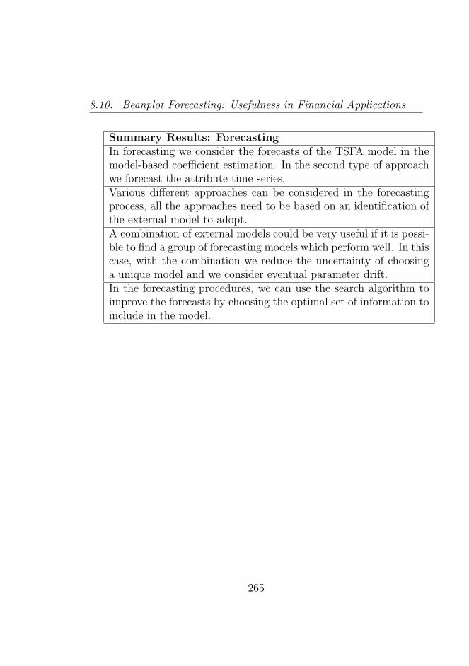
8.10. Beanplot Forecasting: Usefulness in Financial Applications
Summary Results: ForecastingIn forecasting we consider the forecasts of the TSFA model in themodel-based coefficient estimation. In the second type of approachwe forecast the attribute time series.Various different approaches can be considered in the forecastingprocess, all the approaches need to be based on an identification ofthe external model to adopt.A combination of external models could be very useful if it is possi-ble to find a group of forecasting models which perform well. In thiscase, with the combination we reduce the uncertainty of choosinga unique model and we consider eventual parameter drift.In the forecasting procedures, we can use the search algorithm toimprove the forecasts by choosing the optimal set of information toinclude in the model.
265

Chapter 9
Beanplots Time SeriesClustering
A clustering problem is finding similar subgroups of specific items in aspecific set by assuming absence of other information (Jain 2010 [402]and Jain Murty Flynn 1999 [403] Xu Wunsch and others 2005 [708]).In particular the single observations which are the most different be-tween the subgroups and the most similar between each other need tobe considered. There are relevant cases in which the interest is not onlyin analysing one series but groups of series, for example in the case ofthe study of the markets or portfolios(Pattarini Paterlini Minerva 2004[551]). In practice, in these cases, some time series tend to respond toasymmetric shocks similarly (Basalto and De Carlo 2006 [62]). So itis interesting to discriminate the different behaviors over time. Thereare other cases in which the clustering process is not straightforwardbut the series need to be preprocessed. This is the case of complextime series related to phenomena like the financial markets (see Sewell2008 [619] for a review of the characteristics of these series). In thispart we deal with complex time series, represented as beanplot timeseries (BTS).
Beanplots Time Series Clustering
We start from a complex financial time series to obtain the associ-ated beanplot time series (BTS). In particular we start from a seriesyt, t = 1...T with yt ∈ < and we can have a single value in <. Inthe case of the high frequency data we have a huge quantity of ob-servations that need to be aggregated to handle them adequately. Atthe same time high frequency data present irregularities due to thespecific nature of the data (Engle Russell 1998 [253]. In this case weare dealing only with the mean and so we face a loss of information.
Various proposals exist to take into account the internal represen-tations which consider the entire data structure and also the datacenters. There are various proposals in the literature: those dealingwith intervals, histograms (in Arroyo et al. 2011 [38] and 2010 [39])and those dealing with distributions.
All these proposals are related to the field of Symbolic Data Anal-ysis where interval and histograms are particular cases of symbolicdata (see Diday Noirhomme 2008 [218] and Billard and Diday 2003[85]). In Clustering it is very important to retain the relevant datainformation, for this reason we consider the beanplot because it al-lows the retention of the information on the data structures (DragoLauro and Scepi [235] and Drago Scepi 2010 [237]. The density tracein particular gives the chance to take into account structural changesthat can occur. In practice, Beanplot time series (BTS) can representthe features of the initial time series (the beanline corresponds to theaggregated time series). In particular, beanplot can represent at thesame time trend, cycle and even structural changes of the original timeseries. Various clustering approaches for beanplots can be defined:
1. Model approach: Single beanplot or entire time series (RomanoLauro Giordano distance1) see Chapter 9.1
2. Time Series of Attributes (minima, maxima) (Correlation, Cep-
1Romano Giordano Lauro 2006 [594]
268
9.1. Clustering Multiple Beanplot Time Series (BTS): the ModelDistance Approach
stral, Time Warping Distance) Chapter 9.2-9.3
3. Time Series factors of trajectories (Correlation) see Chapter 9.2-9.3
4. Model Based Clustering (Model Based) see Chapter 9.4-9.5
5. Clustering Beanplots Data with Contiguity Constraints Chapter9.6
6. Single Beanplot (Wesserstein ad Euclidean distance) see ChapterChapter 9.7
7. Building Beanplot Prototypes (BPP) using Clustering BeanplotTime Series (BTS) Chapter 9.9
8. Ensemble Clustering see Chapter 9.10
The first method is analyzed in Chapter 9.1 and the others in Chap-ter 9.2-9.10. The different methods reflect the differences in the ap-proaches seen in the internal modelling of the beanplot time series(BTS).
9.1 Clustering Multiple Beanplot Time
Series (BTS): the Model Distance Ap-
proach
Internal Models in this case are sequences of mixture coefficients. Inorder to cluster multiple time series of beanplot Byt with t = 1 . . . T westart from a synthesis of such multiple time series obtained by a mul-tiple factor time series approach ξv,t. In particular we use a suitable
269
Beanplots Time Series Clustering
distance between models, combining a convex function of the differ-ences in model coefficients with corresponding fitting indexes (RomanoGiordano Lauro 2006 [594]).
In order to cluster multiple time series of beanplot Byt with t =1 . . . T starting from the model synthesis, the final aim is to recognizesimilar factor time series with similar dynamics. Thus we obtain thefactorial time series ξv,t and we compute the dissimilarity matrix. Sowe use an adequate distance, as for example, the distance from mod-els in Romano, Giordano Lauro (2006) [594] where we are trying toconsider the dynamics of the different factors.
In order to cluster a set of beanplot time series (BTS) Byt witht = 1 . . . T , we use a suitable distance between models that combinea convex function of the differences in model coefficients with corre-sponding fitting indexes (Romano Giordano Lauro 2006 [594]).Following Signoriello 2008 [630] the two pieces of information are com-bined to define the following measure:
IM(pj, pj′|λ) = λIMP + (1− λ)IMR (9.1)
with λ ∈ [0, 1]. The IM measure is a convex combination of twoquantities IMP and IMR, where IMP is the L2-norm between theestimated coefficients:
IMP =
[∑K−1
k=1
(wjk − wj
′k
)2] 1
2
(j 6= j′) (9.2)
and IMR is the L1-norm between the chi square:
IMR =∣∣∣wjK − wj′K∣∣∣ (j 6= j′). (9.3)
In the clustering process of beanplot time series (BTS) (The two pieces of information are combined to define the following
measure:
270
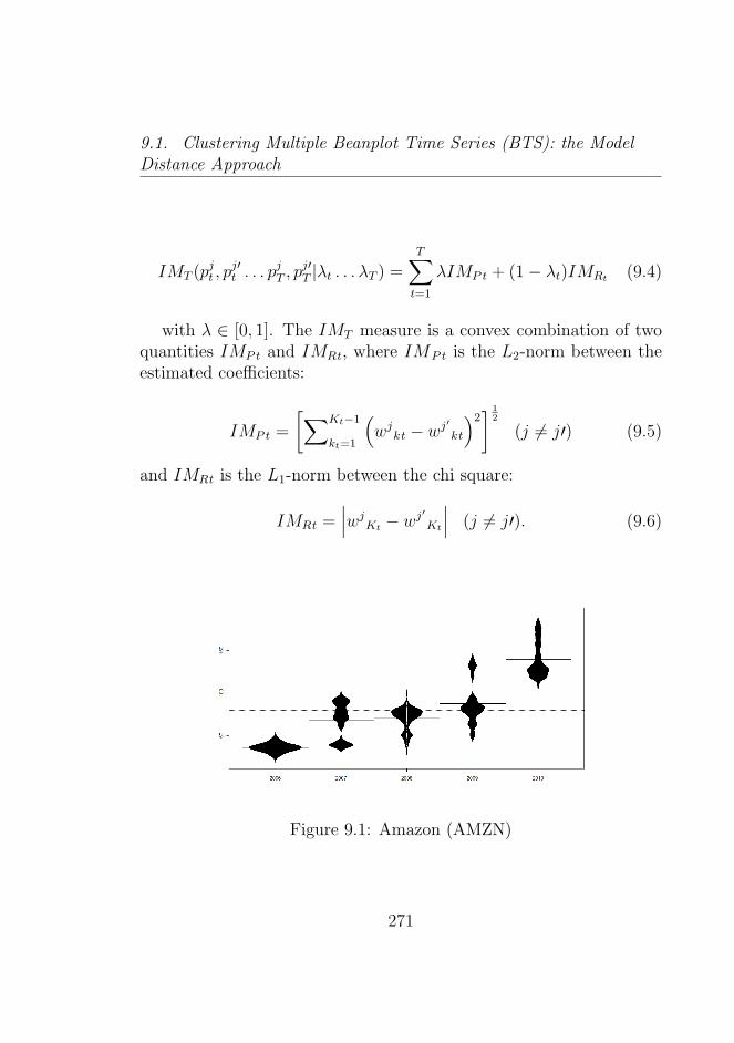
9.1. Clustering Multiple Beanplot Time Series (BTS): the ModelDistance Approach
IMT (pjt , pj′t . . . p
jT , p
j′T |λt . . . λT ) =
T∑t=1
λIMP t + (1− λt)IMRt (9.4)
with λ ∈ [0, 1]. The IMT measure is a convex combination of twoquantities IMP t and IMRt, where IMP t is the L2-norm between theestimated coefficients:
IMP t =
[∑Kt−1
kt=1
(wjkt − wj
′kt
)2] 1
2
(j 6= j′) (9.5)
and IMRt is the L1-norm between the chi square:
IMRt =∣∣∣wjKt − wj
′Kt
∣∣∣ (j 6= j′). (9.6)
Figure 9.1: Amazon (AMZN)
271
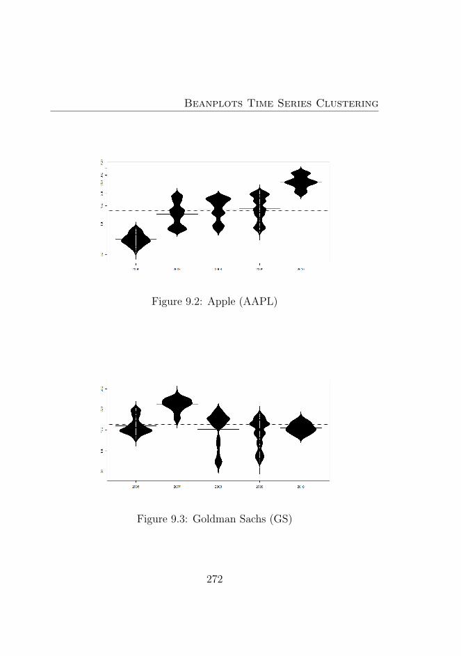
Beanplots Time Series Clustering
Figure 9.2: Apple (AAPL)
Figure 9.3: Goldman Sachs (GS)
272
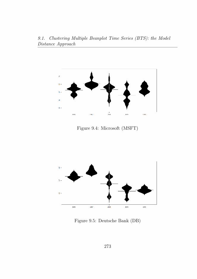
9.1. Clustering Multiple Beanplot Time Series (BTS): the ModelDistance Approach
Figure 9.4: Microsoft (MSFT)
Figure 9.5: Deutsche Bank (DB)
273
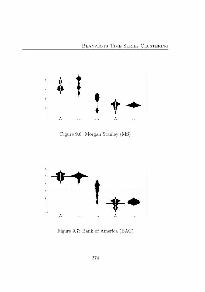
Beanplots Time Series Clustering
Figure 9.6: Morgan Stanley (MS)
Figure 9.7: Bank of America (BAC)
274
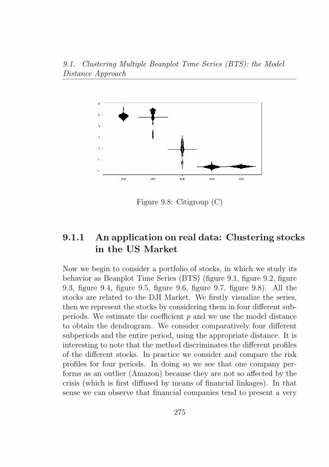
9.1. Clustering Multiple Beanplot Time Series (BTS): the ModelDistance Approach
Figure 9.8: Citigroup (C)
9.1.1 An application on real data: Clustering stocksin the US Market
Now we begin to consider a portfolio of stocks, in which we study itsbehavior as Beanplot Time Series (BTS) (figure 9.1, figure 9.2, figure9.3, figure 9.4, figure 9.5, figure 9.6, figure 9.7, figure 9.8). All thestocks are related to the DJI Market. We firstly visualize the series,then we represent the stocks by considering them in four different sub-periods. We estimate the coefficient p and we use the model distanceto obtain the dendrogram. We consider comparatively four differentsubperiods and the entire period, using the appropriate distance. It isinteresting to note that the method discriminates the different profilesof the different stocks. In practice we consider and compare the riskprofiles for four periods. In doing so we see that one company per-forms as an outlier (Amazon) because they are not so affected by thecrisis (which is first diffused by means of financial linkages). In thatsense we can observe that financial companies tend to present a very
275
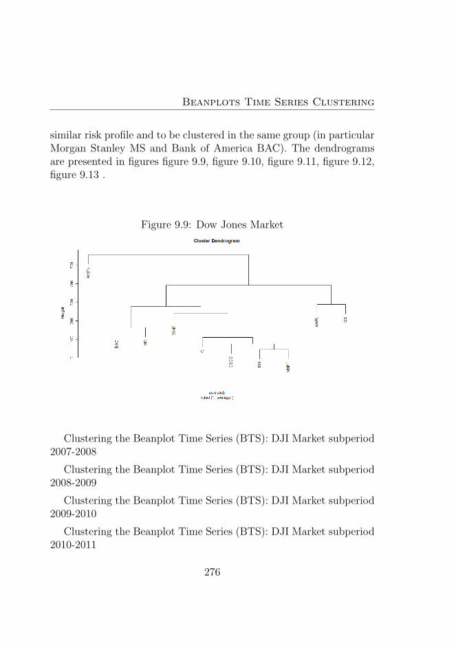
Beanplots Time Series Clustering
similar risk profile and to be clustered in the same group (in particularMorgan Stanley MS and Bank of America BAC). The dendrogramsare presented in figures figure 9.9, figure 9.10, figure 9.11, figure 9.12,figure 9.13 .
Figure 9.9: Dow Jones Market
Clustering the Beanplot Time Series (BTS): DJI Market subperiod2007-2008
Clustering the Beanplot Time Series (BTS): DJI Market subperiod2008-2009
Clustering the Beanplot Time Series (BTS): DJI Market subperiod2009-2010
Clustering the Beanplot Time Series (BTS): DJI Market subperiod2010-2011
276
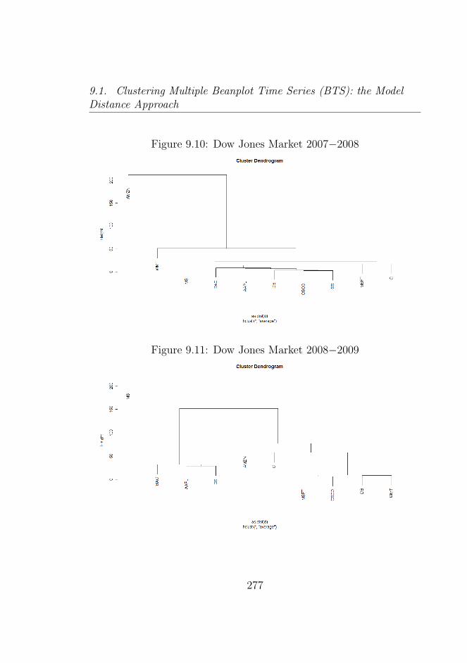
9.1. Clustering Multiple Beanplot Time Series (BTS): the ModelDistance Approach
Figure 9.10: Dow Jones Market 2007−2008
Figure 9.11: Dow Jones Market 2008−2009
277
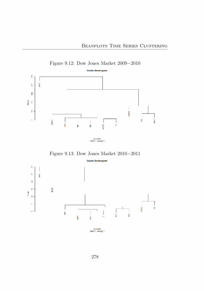
Beanplots Time Series Clustering
Figure 9.12: Dow Jones Market 2009−2010
Figure 9.13: Dow Jones Market 2010−2011
278
9.2. Internal Modelling and Clustering: the Attribute Time SeriesApproach
9.2 Internal Modelling and Clustering: the
Attribute Time Series Approach
In the internal modelling phase it is relevant to choose the bandwidthh for the beanplot time series (BTS) and the number of descriptorpoints or features considered n. We need to select the h parameterfor the entire beanplot series (in order to visualize the series thereis no need to choose the h parameter selected by the Sheather-Jonesmethod). The choice is related to the structure of the data in eachtemporal interval t. The feature n represents both the data structureof the interval temporal and the beanplot evolutive dynamics over timeby its attribute time series. In particular, we have to characterize thebeanplot by considering either the XC and the XC as coordinates. Inthat way we obtain the internal model of the single beanplot at theinterval t. As output of the internal modelling process we obtain theattributes time series for the XC and the Y C of the beanplot time se-ries (BTS). By deciding the number of features n to take into account(for example for XC the 25, 50 and 75th quantile and the related Y C
coordinates (Drago Lauro Scepi 2009 [233]) we have a higher numberof attribute time series). We choose these coordinates without consid-ering the extreme values that could be affected by outliers. The crucialpoint in the internal modelling process is the choice of the bandwidthh and the choice of the number of the n features, considering them inrelation to the data structure. It is important to validate the inter-nal model (the n choice of the features and the chosen bandwidth h)and its adequacy to represent initial data. In general it is necessaryto take into account a lower bandwidth h in the series with a highernumber of features n if there is a higher level of observations: thus, wecan capture a higher number of features. In particular, we considerthat the higher the complexity of the original time series the higherthe complexity requested and the number of features to be taken into
279
Beanplots Time Series Clustering
account. Therefore, it is necessary for most of the cases to reproducethe structure of the beanplot by considering at least three descriptorsfor the XC and three descriptors for the Y C .
9.3 Classical Approaches in Clustering Bean-
plot Features
A first approach, if we are interested in one or more specific attributetime series (for example the attribute of the minima to compare thebehavior in crisis), is that of directly clustering the attribute seriesof the different beanplot time series (BTS) (Algorithm 12). In thissense classical distances can be used, like the Correlation distance,the Cepstral distance, and the Time Warp: see Liao 2005 [455].
At the same time if we need to cluster the entire beanplot time series(BTS) we need to synthesyze and to model (the external model) allthe attribute time series. In particular we use the time series factoranalysis (TSFA) depicted in Meijer Gilbert 2005 [500] and GilbertMeijer 2006 [306] to estimate the attribute time series both for the XC
and for Y C . We start from the n observed processes ai,t with i = 1..nand t = 1..T , where we search from the k unobserved processes (thefactors) ξi,t with t = 1..T and i = 1..k and we obtain the measurementmodel:
at = α + V ξt + εt (9.7)
Where α is a vector of intercepts, V is an n, k matrix of factorloadings and ε is an n vector of random errors. Each factor score rep-resents a measurement model of a latent variable that is the underlyingphenomena of interest. At the end of the procedure we obtain a setof Factors for each attribute time series. For the measurement of thefactor score predictor we use the Bartlett predictor, following Meijer
280
9.3. Classical Approaches in Clustering Beanplot Features
Gilbert 2005 [500], Wansbeek and Meijer. (2000) [690] and WansbeekMeijer (2005) [689].
ξt = (V tΨ−1t V )−1V tΨ−1V t(zt − αt) (9.8)
Where: ψt = Cov(εt). The loadings can be estimated by FA es-timators (ML in particular) using the sample covariance of the error(Meijer Gilbert 2005 [500]). We compute one factor time series eitherfor the XC or for the Y C using the attribute time series. Either one ofthe two factorial time series represents the XC and Y C , where the firstone represents the general dynamics of the beanplot (in particular thelocation and the size) and the second one represents the response ofthe shock or the short run dynamics (the shape).
The final aim of the clustering process (Algorithm 13) is to rec-ognize groups of time series with a synchronous dynamic (related tothe location of the beanplot or the XC) and a similar response to theshocks (related to the Y C). Having obtained for each beanplot thefactorial time series both for the XC and the Y C , we compute the dis-similarity matrix. In particular we use three versions of the distanceknown in literature as correlational distances (see for example Doseand Cincotti 2005 [225]), where we try to specifically recognize thecorrelation between the dynamics of the different synthesizing factorsover time. So we have:
d(Y,X) = 1− (cξbYt ,ξbXt) (9.9)
Where: Y = (ξbY1 , ξbY2 , . . . , ξbYt) and X = (ξbX1 , ξbX2 , . . . , ξbXt),and cξbYt ,ξbXt
is the correlation coefficient between the two factorial
time series related to XC and Y C . We use as well2 other correlationaldistances to compare the results:
2See Glynn (2005) [751]
281
Beanplots Time Series Clustering
d(Y,X) =1− (cξbYt ,ξbXt
))
2(9.10)
Considering the absolute values:
d(Y,X) = 1−∣∣(cξbYt ,ξbXt
)∣∣ (9.11)
and finally:
d(Y,X) = 2
√1− (cξbYt ,ξbXt
)2 (9.12)
We obtain the dissimilarity matrices related and we use differentclustering methods to compare the different results. We use the hi-erarchical clustering and the non hierarchical clustering by applyingdifferent methods. At this point we can apply different methods toobserve the robustness of the results.
9.3.1 Application: classifying the synchronous dy-namics of the world indices beanplot timeseries (BTS)
The methods depicted in the previous chapters are transformed in Rprograms and experimented both on simulated data to test the char-acteristics of the methods, and also on real data. In the applicationon real data we consider various time series related to the index ofthe major stockmarkets around the world. In particular we consider14 markets related to different continents. The interval period consid-ered, for the collected data, is the period 2001-2008. As a first step wecompute the beanplot time series (BTS) from the original time series,and we use the information of the bandwidths to explore the volatility(represented over time). Secondly, we identify the bandwidth and wecompute the attribute time series for all the beanplots both for the
282
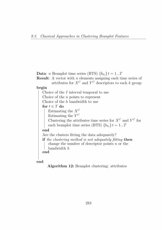
9.3. Classical Approaches in Clustering Beanplot Features
Data: n Beanplot time series (BTS) bYt t = 1...TResult: A vector with n elements assigning each time series of
attributes for XC and Y C descriptors to each k groupbegin
Choice of the I interval temporal to useChoice of the n points to representChoice of the h bandwidth to usefor t ∈ T do
Estimating the XC
Estimating the Y C
Clustering the attributes time series for XC and Y C foreach beanplot time series (BTS) bYt t = 1...T
endAre the clusters fitting the data adequately?if the clustering method is not adequately fitting then
change the number of descriptor points n or thebandwidth h
end
endAlgorithm 12: Beanplot clustering: attributes
283
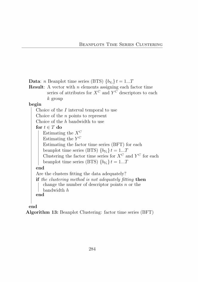
Beanplots Time Series Clustering
Data: n Beanplot time series (BTS) bYt t = 1...TResult: A vector with n elements assigning each factor time
series of attributes for XC and Y C descriptors to eachk group
beginChoice of the I interval temporal to useChoice of the n points to representChoice of the h bandwidth to usefor t ∈ T do
Estimating the XC
Estimating the Y C
Estimating the factor time series (BFT) for eachbeanplot time series (BTS) bYt t = 1...TClustering the factor time series for XC and Y C for eachbeanplot time series (BTS) bYt t = 1...T
endAre the clusters fitting the data adequately?if the clustering method is not adequately fitting then
change the number of descriptor points n or thebandwidth h
end
endAlgorithm 13: Beanplot Clustering: factor time series (BFT)
284
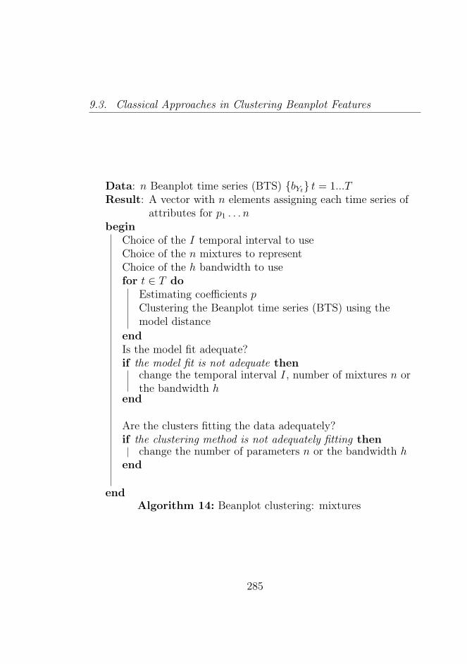
9.3. Classical Approaches in Clustering Beanplot Features
Data: n Beanplot time series (BTS) bYt t = 1...TResult: A vector with n elements assigning each time series of
attributes for p1 . . . nbegin
Choice of the I temporal interval to useChoice of the n mixtures to representChoice of the h bandwidth to usefor t ∈ T do
Estimating coefficients pClustering the Beanplot time series (BTS) using themodel distance
endIs the model fit adequate?if the model fit is not adequate then
change the temporal interval I, number of mixtures n orthe bandwidth h
end
Are the clusters fitting the data adequately?if the clustering method is not adequately fitting then
change the number of parameters n or the bandwidth hend
endAlgorithm 14: Beanplot clustering: mixtures
285
Beanplots Time Series Clustering
XC and the Y C . We consider three specific time series both for theXC and for the Y C . At this point we consider both the true differ-ent groups of time series and we synthesize the time series regardingonly one factor for the XC and one factor for the Y C . We obtain thefactor time series. It is interesting to note the strong impact of thefinancial crisis on all the world stockmarkets jointly, where there arevarious different responses due to the different economic policies. Atthis point we classify the beanplot time series (BTS) and analyse thesynchronous behavior to compute the dissimilarity matrix, by usingdifferent distances. Finally, using different methods we compare theresults obtained from the hierarchical and non hierarchical clusteringprocess. We retain a factor 1, that could be interpreted accordingto size and data location, which determines classification due to thedifferent development characteristics of the different markets. WhereBrazil and Mexico represent the ”developing markets”, other marketscan be considered ”developed” such as the US market. Moreover thedeveloping markets show a better response to the crisis (and they fin-ish in the same cluster with these characteristics) as we can observefrom the factorial time series. More in particular, for the developingmarkets, there is higher growth and instability in the long term buta better response to the financial crisis in the short term. It is in-teresting to note a quick reaction to the crisis by the US and Japandue to the expansionary economic policy and general policies adopted.Hong Kong reacts as a specific market (in particular through its ties toChina) and Sweden represents an isolated market. The second factorY C represents the dynamics of the beanplot shape, and we observefrom the different clusters that there are similarities in the shock re-sponses (representing also the beanplot shape). Markets that are nearthrough their close proximity, in that sense, show similarities in be-haviour due to the financial connection. We expect that markets closein proximity tend to behave similarly, and infact we observe that theclusters present regroupments related to the European markets, the
286
9.4. Model Based Clustering and Modern Framework
Asian markets and ”signal markets” such as Japan and the US. Inparticular the data seems to show that in the short run the geograph-ical factor seems to be fundamental for defining groups for Y C . Theshort run dynamics is strongly related to the shocks and the conta-gion mechanisms. The geographical spread of the shocks occurs ifwe consider financial ties between different markets. For France andSwizerland, in particular, we observe a strong reaction to the shocksand synchronous movement of the markets whereas for the Europeancountries we observe various levels of synchronous movements of themarkets due to their common economic policies and economic shocks.Finally, for the Asian and Latin American countries we find a generalinstability (Brazil Mexico), and a connection between shocks in Asiancountries (Indonesia, Hong Kong, Singapore etc.). The instability ofthe Latin American countries tends to have an impact also on theSpanish market. Finally, Japan and the US are markets that repre-sent ”signals” (which means they tend to behave differently comparedto other markets).
9.4 Model Based Clustering and Modern
Framework
In the first part of the work we have considered classical clusteringmethods based on specific heuristics. Finite Mixture model structurescan be used as well in the clustering process, where, in particular,each single component distribution can be considered a cluster. For areview of these methods in the context of clustering see in particularMelnykov Maitra (2010) [502]. Finite Mixture Models provide the ba-sic foundation for a different approach: the Model Based Clustering(Wolfe 1963 [705]). In this new framework, Bock 1996 [94], FraleyRaftery (2002) [277] and Bock 1998 [92] has proposed a clustering ap-
287
Beanplots Time Series Clustering
proach based on probability models. Clusters, in this approach, can beconsidered a component probability distribution (Fraley Raftery 2002[277]) where the foundation is a formal statistical approach (FraleyRaftery 2007 [279]). Heuristic approaches can be used as approximateestimation methods for some probability models (Fraley Raftery 2002[277]). This second clustering strategy is necessary because of thedata complexity of the behaviours of the original data. In the firstapproach, that is considering the TSFA analysis, we synthesized theinformation, here we want to obtain clusters considering the differentbehaviors of the different XC and Y C (at a lower or a higher level). Inthis sense we are taking into account the data complexity and we con-sider the different features of the beanplot behavior over time in theclustering process. In particular we consider n time series of beanplotscharacterized by different features XC − Y C . Each feature XC − Y C
can be seen as a single representation and could be differently mod-elled considering the different time series. Another important ideaunderlying this approach is that by considering subperiods over timewe observe the change over time of the data structure and the mod-els. So we are considering data-analysis not as a photograph of thesituation but as the specific dynamics of change over time (followingan approach in a different context like Riani 2004 [582]).
9.5 Feature Model Based Clustering for
Beanplot Time Series (BTS)
The procedure can be defined in some sequential steps: in a commonway with respect to the TSFA methodology of beanplot clustering,we had to define the set of the attribute time series. We obtain, forexample (the higher the level of definition we choose the higher thenumber of descriptor points) six descriptor points of three XC and
288
9.5. Feature Model Based Clustering for Beanplot Time Series(BTS)
three Y C for each time. Having obtained the attribute time serieswe consider each couple of XC − Y C attributes. Optionally we canchoose an aggregation subperiod in which we can obtain a specificvalue XC−Y C for the beanplot time series (BTS) for the entire period(or for a subperiod). We perform the model based clustering procedurefor each couple of characteristics considered (Algorithm 15) in thesubperiod and we obtain the clustering model and the classificationfor each feature. It is important to note that the expectation is thatthe beanplot time series (BTS) will be different in their features andcharacteristics over time.
In fact, some attribute series tend to perform differently over timet (for example, different minima and maxima) and beanplot featurescan capture these differences. As already stated in the first part of thework, in the Y C features we are considering the variability or the shortrun movements, in the XC attribute time series we are considering themean effect over time, or the long run dynamics. Here, following FraleyRaftery 2002 [277], we perform a model based cluster analysis for thedifferent beanplot XC − Y C features, each considered as a temporalobservation. Following Fraley and Raftery 2007 [279], we are makingthe important assumption that in a specific set of data, the observationz (related to the a feature XC−Y C) is generated by a mixture density:
f(z) =G∑p=1
τpfp(z) (9.13)
where τp with (τp ∈ (0, 1) and∑G
p τp = 1) and fp as a probabilitydensity function of the observations belong in the group p. The meanµp and the covariance matrix
∑p of the component distributions have
the probability density function:
φ(zi;µp,Σp) =exp
−1
2(zi − µp)TΣ−1
p (zi − µp)√
det(2πΣp)(9.14)
289
Beanplots Time Series Clustering
The likelihood for the considered data is:
n∏i=1
G∑p=1
τpφ(xi;µp; Σp) (9.15)
Here, the parameters (τp, µpΣp) are estimated by using the EM al-gorithm. The mean, µp and the covariance matrix Σp characterize thedifferent components. In particular, Covariances Σp fix the geometricfeatures of the clusters, especially the shape, the volume and the ori-entation. In this sense, the authors, Celeux Govaert (1995) [125], Fra-ley Raftery (1998) [275] and Fraley Raftery (2002) [277] proposed tospecifically parametrize the group covariance matrices through eigen-value decomposition of the Gaussian Mixture Model:
Σp = λpDpApDTp (9.16)
Where in particular: Dp is the orthogonal matrix consisting of theeigenvectors, Ap is a diagonal matrix with entries proportional to theeigenvalues of Σp, and λp is an associated scalar constant to the el-lipsoid volume (Fraley 1996 [274]). The geometric characteristics ofthe components are discovered when the parameters are found (FraleyRaftery 2007 [279] and Raftery Fraley 2007 [571]) in particular Dp
the orientation of the specific component p of the mixture, Ap rep-resents the shape, whilst λp represents the volume. It is importantto note that we obtain different models over time. So we repeat themodel-based clustering for each subperiod but also for each couple offeatures XC − Y C . The general estimation method of the parametersis the EM algorithm that shows the different shape of the mixtures aswell (for an adequate categorization of the different models see Fra-ley Raftery 2002 [277]). In general the EM algorithm is a statisticaltool in mixture estimation problems or also those involving missingdata (Borman 2009 [103]). The EM algorithm can be considered as
290
9.5. Feature Model Based Clustering for Beanplot Time Series(BTS)
a procedure structured in two distinct parts. In the ”E” part, theconditional expectation of the complete data log-likelihood is com-puted cosidering the data, with parameter estimates (following FraleyRaftery 2002 [277]). In the ”M” part, the parameters maximizingthe expected log-likelihood (from the antecedent ”E” part) are com-puted. It is necessary in our context to repeat the analysis for thedifferent beanplot features (or attributes) considered. The algorithmtends to converge if the increases of the likelihood in the sequential it-erations increase (for each feature considered) Borman 2009 [103] andalso Fraley Raftery 2002 [277]. At the end of the procedure we obtainthe parametrizations of the different models (see also Fraley Raftery1999 [276]). By obtaining the parameters it is possible to show thestructure of the components (Fraley Raftery 1998 [275]), the differ-ent parameterizations of the covariance matrix are shown in (FraleyRaftery 2006 [278]). Moreover, where each cluster corresponds to adifferent statistical model (Fraley Raftery 2002 [277]), a typical modelselection, the problem is to choose the number of partitions or clustersin the model based clustering process. For the model selection, variousmethods can be used (see Fraley Raftery 2002 [277]), one of the mostknown in literature is the BIC (see Fraley Raftery 1999 [276]). So wechoose the model that maximizes the BIC index for every beanplotfeature, because a penalty term is added to the number of parametersof the log-likelihood considered. As the authors state (Fraley Raftery2002 [277]) there is a specific trade-off in selecting a simple model or acomplex one. The second calls, usually, for a lower number of clusters.
9.5.1 The choice of the temporal windows
The choice of the temporal interval to be used in the dynamic partof the procedure is a decision linked to the objectives of the analysis.In particular, it can be interesting to compare the model based clus-tering process in two (or more) different subperiods, alternatively it
291
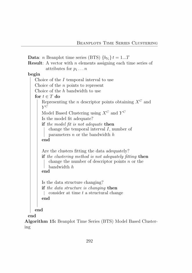
Beanplots Time Series Clustering
Data: n Beanplot time series (BTS) bYt t = 1...TResult: A vector with n elements assigning each time series of
attributes for p1 . . . nbegin
Choice of the I temporal interval to useChoice of the n points to representChoice of the h bandwidth to usefor t ∈ T do
Representing the n descriptor points obtaining XC andY C
Model Based Clustering using XC and Y C
Is the model fit adequate?if the model fit is not adequate then
change the temporal interval I, number ofparameters n or the bandwidth h
end
Are the clusters fitting the data adequately?if the clustering method is not adequately fitting then
change the number of descriptor points n or thebandwidth h
end
Is the data structure changing?if the data structure is changing then
consider at time t a structural changeend
end
endAlgorithm 15: Beanplot Time Series (BTS) Model Based Cluster-ing
292
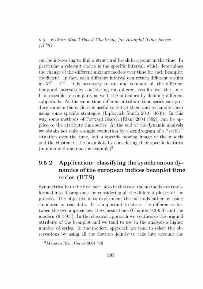
9.5. Feature Model Based Clustering for Beanplot Time Series(BTS)
can be interesting to find a structural break in a point in the time. Inparticular a relevant choice is the specific interval, which determinesthe change of the different mixture models over time for each beanplotcoefficient. In fact, each different interval can return different resultsin XC − Y C . It is necessary to run and compare all the differenttemporal intervals by considering the different results over the time.It is possible to compare, as well, the outcomes by defining differentsubperiods. At the same time different attribute time series can pro-duce some outliers. So it is useful to detect them and to handle themusing some specific strategies (Lipkovich Smith 2010 [463]). In thisway some methods of Forward Search (Riani 2004 [582]) can be ap-plied to the attribute time series. At the end of the dynamic analysiswe obtain not only a single evaluation by a dendrogram of a ”stable”situation over the time, but a specific moving image of the modelsand the clusters of the beanplots by considering their specific features(minima and maxima for example)3.
9.5.2 Application: classifying the synchronous dy-namics of the european indices beanplot timeseries (BTS)
Symmetrically to the first part, also in this case the methods are trans-formed into R programs, by considering all the different phases of theprocess. The objective is to experiment the methods either by usingsimulated or real data. It is important to stress the differences be-tween the two approaches: the classical one (Chapter 9.2-9.3) and themodern (9.4-9.5). In the classical approach we synthesize the originalattribute of the beanplot and we tend to use in the analysis a highernumber of series. In the modern approach we tend to select the ob-servations by using all the features jointly to take into account the
3Atkinson Riani Cerioli 2004 [48]
293
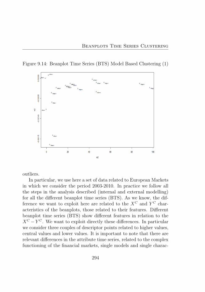
Beanplots Time Series Clustering
Figure 9.14: Beanplot Time Series (BTS) Model Based Clustering (1)
outliers.In particular, we use here a set of data related to European Markets
in which we consider the period 2003-2010. In practice we follow allthe steps in the analysis described (internal and external modelling)for all the different beanplot time series (BTS). As we know, the dif-ference we want to exploit here are related to the XC and Y C char-acteristics of the beanplots, those related to their features. Differentbeanplot time series (BTS) show different features in relation to theXC − Y C . We want to exploit directly these differences. In particularwe consider three couples of descriptor points related to higher values,central values and lower values. It is important to note that there arerelevant differences in the attribute time series, related to the complexfunctioning of the financial markets, single models and single charac-
294
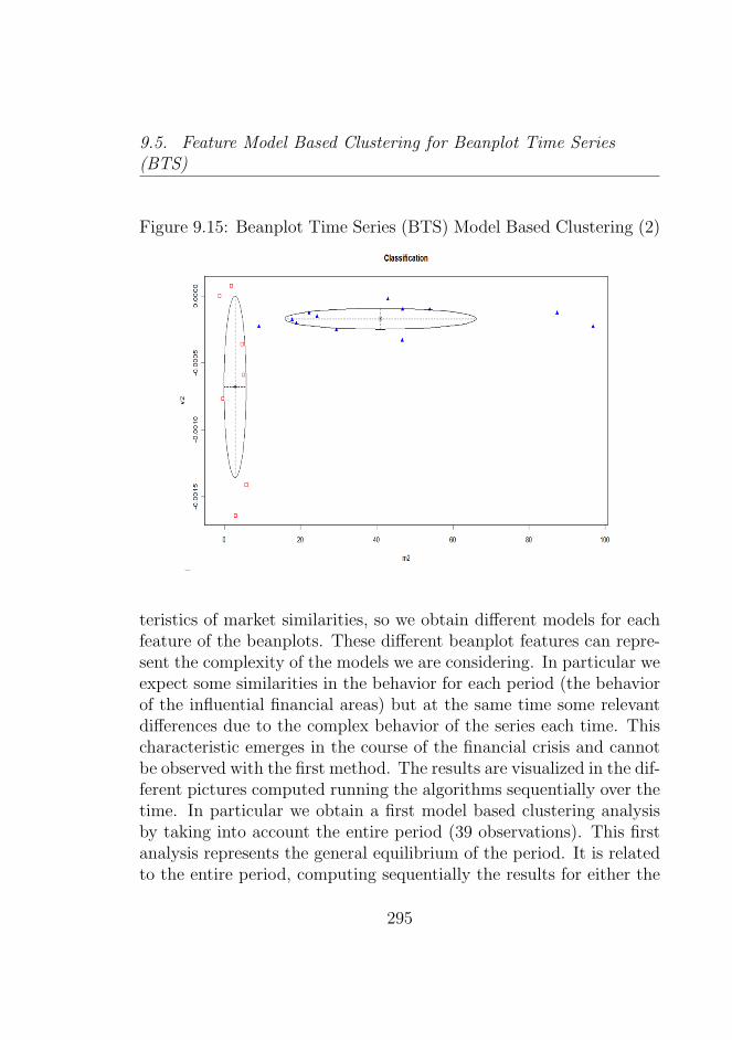
9.5. Feature Model Based Clustering for Beanplot Time Series(BTS)
Figure 9.15: Beanplot Time Series (BTS) Model Based Clustering (2)
teristics of market similarities, so we obtain different models for eachfeature of the beanplots. These different beanplot features can repre-sent the complexity of the models we are considering. In particular weexpect some similarities in the behavior for each period (the behaviorof the influential financial areas) but at the same time some relevantdifferences due to the complex behavior of the series each time. Thischaracteristic emerges in the course of the financial crisis and cannotbe observed with the first method. The results are visualized in the dif-ferent pictures computed running the algorithms sequentially over thetime. In particular we obtain a first model based clustering analysisby taking into account the entire period (39 observations). This firstanalysis represents the general equilibrium of the period. It is relatedto the entire period, computing sequentially the results for either the
295
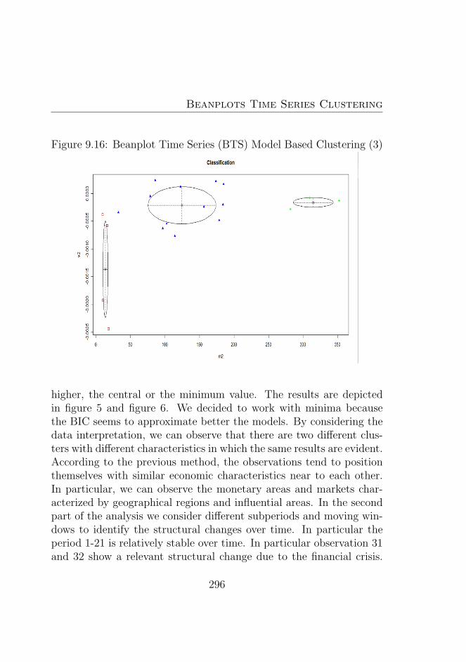
Beanplots Time Series Clustering
Figure 9.16: Beanplot Time Series (BTS) Model Based Clustering (3)
higher, the central or the minimum value. The results are depictedin figure 5 and figure 6. We decided to work with minima becausethe BIC seems to approximate better the models. By considering thedata interpretation, we can observe that there are two different clus-ters with different characteristics in which the same results are evident.According to the previous method, the observations tend to positionthemselves with similar economic characteristics near to each other.In particular, we can observe the monetary areas and markets char-acterized by geographical regions and influential areas. In the secondpart of the analysis we consider different subperiods and moving win-dows to identify the structural changes over time. In particular theperiod 1-21 is relatively stable over time. In particular observation 31and 32 show a relevant structural change due to the financial crisis.
296
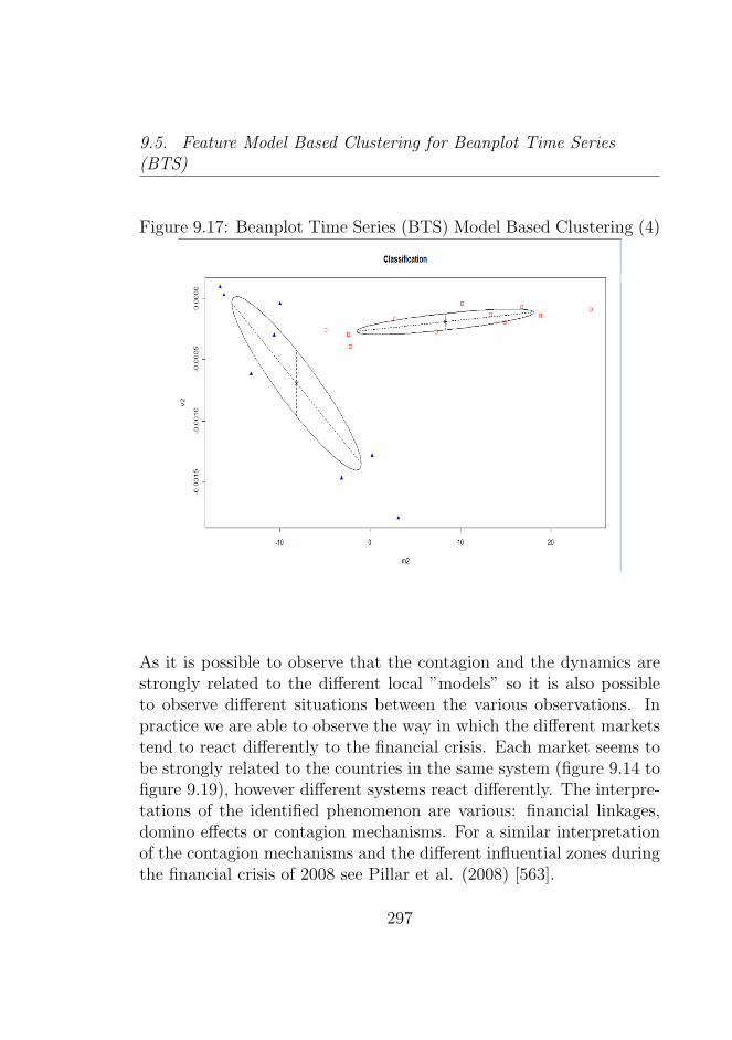
9.5. Feature Model Based Clustering for Beanplot Time Series(BTS)
Figure 9.17: Beanplot Time Series (BTS) Model Based Clustering (4)
As it is possible to observe that the contagion and the dynamics arestrongly related to the different local ”models” so it is also possibleto observe different situations between the various observations. Inpractice we are able to observe the way in which the different marketstend to react differently to the financial crisis. Each market seems tobe strongly related to the countries in the same system (figure 9.14 tofigure 9.19), however different systems react differently. The interpre-tations of the identified phenomenon are various: financial linkages,domino effects or contagion mechanisms. For a similar interpretationof the contagion mechanisms and the different influential zones duringthe financial crisis of 2008 see Pillar et al. (2008) [563].
297
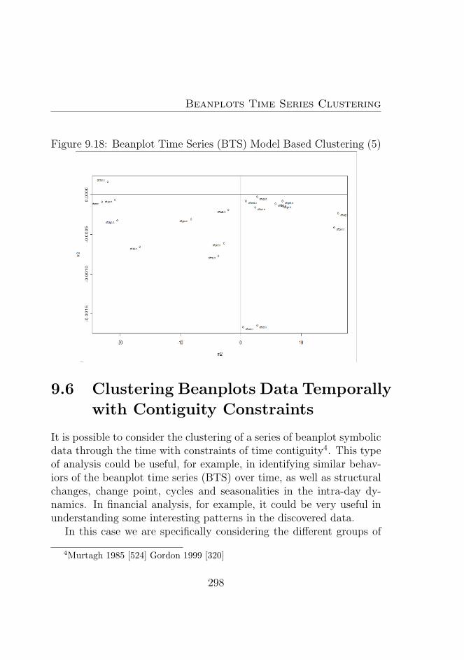
Beanplots Time Series Clustering
Figure 9.18: Beanplot Time Series (BTS) Model Based Clustering (5)
9.6 Clustering Beanplots Data Temporally
with Contiguity Constraints
It is possible to consider the clustering of a series of beanplot symbolicdata through the time with constraints of time contiguity4. This typeof analysis could be useful, for example, in identifying similar behav-iors of the beanplot time series (BTS) over time, as well as structuralchanges, change point, cycles and seasonalities in the intra-day dy-namics. In financial analysis, for example, it could be very useful inunderstanding some interesting patterns in the discovered data.
In this case we are specifically considering the different groups of
4Murtagh 1985 [524] Gordon 1999 [320]
298
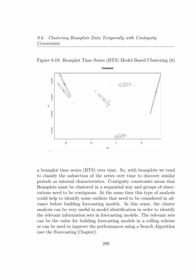
9.6. Clustering Beanplots Data Temporally with ContiguityConstraints
Figure 9.19: Beanplot Time Series (BTS) Model Based Clustering (6)
a beanplot time series (BTS) over time. So, with beanplots we tendto classify the subsection of the series over time to discover similarperiods as internal characteristics. Contiguity constraints mean thatBeanplots must be clustered in a sequential way and groups of obser-vations need to be contiguous. At the same time this type of analysiscould help to identify some outliers that need to be considered in ad-vance before building forecasting models. In this sense, the clusteranalysis can be very useful in model identification in order to identifythe relevant information sets in forecasting models. The relevant setscan be the value for building forecasting models in a rolling schemeor can be used to improve the performances using a Search Algorithm(see the Forecasting Chapter).
299
Beanplots Time Series Clustering
9.7 Clustering using the Wesserstein Dis-
tance
Following Irpino and Verde 2008 ([398]), the authors propose theWesserstein distance to cluster histograms. The same distance canbe used to cluster the density data. In particular the Wesserstein L2metric is proposed in Gibbs and Su (2002) [305].
Where the quantile functions of the two distributions are F−1i and
F−1j so we use this distance:
dW (Byi, Byj
) =
√∫ 1
0
F−1i (t)− F−1
j (t) dt (9.17)
At the same time Irpino and Romano (2007) [395] have proved thatthe distance can be decomposed as:
d2W = (µi − µj)2 + (σi − σj)2 + σiσj(1− ρQQ(Fi, Fj)) (9.18)
Where ρQQ(Fi, Fj) can be considered the correlation of the quantilesof the two distributions Fi and Fj that could be considered in theclassical QQ plot. In particular by using this distance we can classifythe single density data, where we compute the dissimilarity matrix(Algorithm 16. So in that sense, we consider various different methodsto classify the different beanplots over time.
300
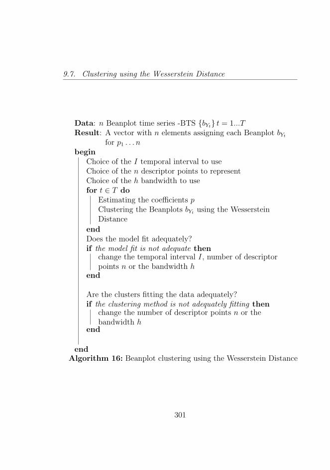
9.7. Clustering using the Wesserstein Distance
Data: n Beanplot time series -BTS bYt t = 1...TResult: A vector with n elements assigning each Beanplot bYt
for p1 . . . nbegin
Choice of the I temporal interval to useChoice of the n descriptor points to representChoice of the h bandwidth to usefor t ∈ T do
Estimating the coefficients pClustering the Beanplots bYt using the WessersteinDistance
endDoes the model fit adequately?if the model fit is not adequate then
change the temporal interval I, number of descriptorpoints n or the bandwidth h
end
Are the clusters fitting the data adequately?if the clustering method is not adequately fitting then
change the number of descriptor points n or thebandwidth h
end
endAlgorithm 16: Beanplot clustering using the Wesserstein Distance
301
Beanplots Time Series Clustering
9.8 Comparative Approaches: Clustering
beanplots from Attribute Time Se-
ries
The different methods seen are related to different objectives and be-long to different approaches. In the case of the coefficients estimationbased on mixtures the objective is to cluster specifically the models(internal models) so the appropriate distance is the distance of Ro-mano Lauro Giordano 1996 [594]. In general this type of coefficientsestimation is related to the differences between different beanplotsover time, and can be compared by considering different subperiods inthe beanplot time series (BTS) where the objective is to cluster eachmodel, separately considered, in the series of the beanplots. In thatsense we are clustering the structural part of the beanplots. Here weuse the coefficients estimation related to the mixtures
A completely different approach is that related to considering thetrajectories of the beanplot and its synthesis. Here the representationconsidered is related to the coordinates. In that sense we can considerthe factor time series of the beanplot time series (BTS) and we usethe appropriate distance to cluster the different time series. In thiscase we are considering the different temporal evolution of the differ-ent series. We define this method as the ”classical” one.
A modern approach is Model based clustering. In this case we areconsidering both the XC the Y C for each beanplot time series (BTS).Clearly also in this case we consider the representation by coordinates.In this case we consider also for each time the specific representation.
Finally, if the interest is to cluster each beanplot data in a beanplottime series (BTS) we can consider the different beanplot and clusterthe beanplots using other types of distances such as Euclidean or theWesserstein distance.
302
9.9. Building Beanplot Prototypes (BPP) using Clustering BeanplotTime Series (BTS)
9.9 Building Beanplot Prototypes (BPP)
using Clustering Beanplot Time Se-
ries (BTS)
A relevant Clustering application is to build prototypes (or indica-tors) from the original Beanplot Time Series (BTS)(Algorithm 17,Algorithm 18 and figure 9.20). In particular we start from the origi-nal Beanplot time series (BTS) which we parameterize following thetwo different approaches (coefficients estimation At and coordinatesXC and Y C). So we obtain the Factor Time Series (defined BFT)by the Time series factor analysis methodology. In this sense we aresynthesizing the information in the beanplots and we are consideringthe latent factors which impact on the beanplot dynamics. Then wecan use a clustering technique to obtain clusters of time series andhis prototypes. These prototypes are very useful to build indicatorsfor the initial beanplot time series (BTS) related to specific groupswith similar dynamics (for example starting from the Beanplot timeseries (BTS) related to different stocks it is possible to build indica-tors related to stocks with similar behaviors). At the same time theprototypes are useful in the Forecasting processes where it is possi-ble to identify different Beanplot time series (BTS) which could bemodelled to take into account the specific inter-relationships betweenthem. Beanplot Time Series (BTS) which act as outliers can be welldetected in this way.
9.10 Sensitivity and Robustness of the Clus-
tering Methods
The outlier identification is a relevant but not simple task (see Huber1981 [373]). So a first possible outcome in the cluster analysis is that
303
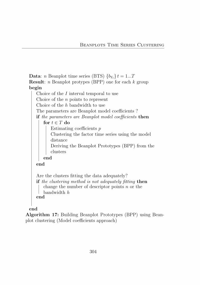
Beanplots Time Series Clustering
Data: n Beanplot time series (BTS) bYt t = 1...TResult: n Beanplot protypes (BPP) one for each k groupbegin
Choice of the I interval temporal to useChoice of the n points to representChoice of the h bandwidth to useThe parameters are Beanplot model coefficients ?if the parameters are Beanplot model coefficients then
for t ∈ T doEstimating coefficients pClustering the factor time series using the modeldistanceDeriving the Beanplot Prototypes (BPP) from theclusters
end
end
Are the clusters fitting the data adequately?if the clustering method is not adequately fitting then
change the number of descriptor points n or thebandwidth h
end
endAlgorithm 17: Building Beanplot Prototypes (BPP) using Bean-plot clustering (Model coefficients approach)
304
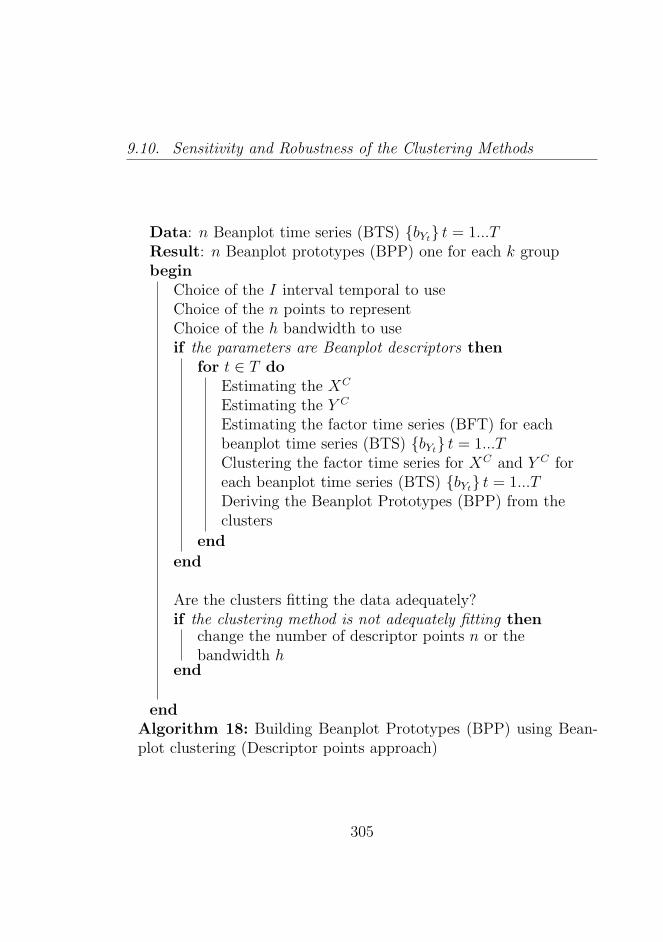
9.10. Sensitivity and Robustness of the Clustering Methods
Data: n Beanplot time series (BTS) bYt t = 1...TResult: n Beanplot prototypes (BPP) one for each k groupbegin
Choice of the I interval temporal to useChoice of the n points to representChoice of the h bandwidth to useif the parameters are Beanplot descriptors then
for t ∈ T doEstimating the XC
Estimating the Y C
Estimating the factor time series (BFT) for eachbeanplot time series (BTS) bYt t = 1...TClustering the factor time series for XC and Y C foreach beanplot time series (BTS) bYt t = 1...TDeriving the Beanplot Prototypes (BPP) from theclusters
end
end
Are the clusters fitting the data adequately?if the clustering method is not adequately fitting then
change the number of descriptor points n or thebandwidth h
end
endAlgorithm 18: Building Beanplot Prototypes (BPP) using Bean-plot clustering (Descriptor points approach)
305
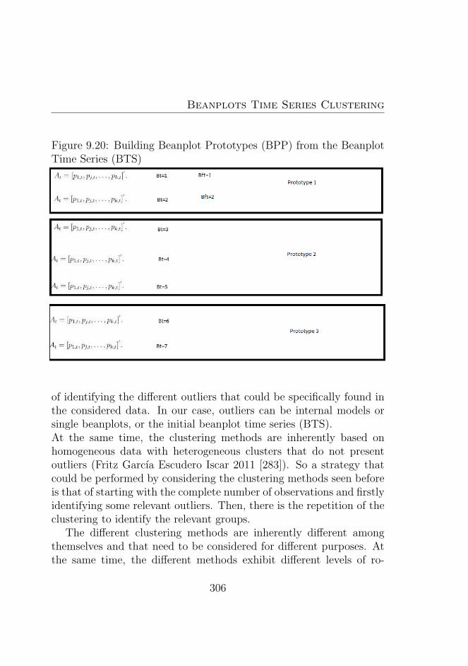
Beanplots Time Series Clustering
Figure 9.20: Building Beanplot Prototypes (BPP) from the BeanplotTime Series (BTS)
of identifying the different outliers that could be specifically found inthe considered data. In our case, outliers can be internal models orsingle beanplots, or the initial beanplot time series (BTS).At the same time, the clustering methods are inherently based onhomogeneous data with heterogeneous clusters that do not presentoutliers (Fritz Garcıa Escudero Iscar 2011 [283]). So a strategy thatcould be performed by considering the clustering methods seen beforeis that of starting with the complete number of observations and firstlyidentifying some relevant outliers. Then, there is the repetition of theclustering to identify the relevant groups.
The different clustering methods are inherently different amongthemselves and that need to be considered for different purposes. Atthe same time, the different methods exhibit different levels of ro-
306
9.11. Clustering: Usefulness in Financial Applications
bustness they need to be considered both with or without the outliersfound previously in the analysis of identifying the data structures.
An alternative is the use of a robust method in clustering alongone of the approaches followed in literature (see Hardin Rocke 2004[339] Garcıa-Escudero, Gordaliza, and Matran, C. (2003) [292] and fordifferent approaches Henning 2009 [357] and Riani 2004 [582])
9.10.1 Ensemble Strategies in Clustering Bean-plots
Another possible approach to improve the quality and the robustnessof the cluster solutions in the clustering process is to adopt an ensem-ble strategy (see Day 1986 [171], Hornik 2005 [366], Strehl and Ghosh2002 [643]). In practice it is possible to use different clustering meth-ods and reconcile the information obtained by the different methods(Consensus Clustering).
In particular in the beanplot time series (BTS) it is possible to clus-ter by considering different methods (both clustering the time seriesof beanplots, or the single internal data) so we can use the ensemblemethods to assess the stability of the clusters obtained.
In this sense, we can consider as input type in the ensamble clus-tering the following: the different internal modelling approaches, thedifferent distances and the different methods explored above duringthe chapter, with the aim of comparing the results between them.
9.11 Clustering: Usefulness in Financial
Applications
Clustering Beanplots time series can be useful in different contexts.For example, it is possible to monitor the behavior of different stocks
307
Beanplots Time Series Clustering
to determine the subset of the stocks determining the weight of eachstock in the portfolio (for asset allocation purposes). So in this sensethe characteristic of the beanplot time series (BTS) is that of usinga high quantity of available information to cover different possibleevents in order to choose the different subset of stocks under differenttemporal contexts. At the same time it is possible to apply cluster-ing techniques to evaluate the differences between stocks. It is alsopossible to identify the different market phases by considering a clus-tering technique with contiguity constraint. We obtain a contiguousseries of the most similar beanplots by segmenting the initial beanplottime series (BTS) to indicate different market phases. Therefore it ispossible to detect the different market phases and to determine whichtype of events is causing the stock behavior. The beanplot can takeinto account volatility and so this can be a tool for financial risk man-agement. At the same time, the beanplot can be useful in statisticalarbitrage in order to identify very similar pairs of different stocks (seeChapter 11).
Possible applications: Market Monitoring, Macroeconomic and Fi-nancial Analysis, Mining Financial Data, Statistical Arbitrage, AssetAllocation, Quantitative Trading−event identification, Event Studies,identifying patterns related to specific financial events in a tempo-ral window, Tactical Asset Allocation−pattern identification and ex-ploitation (using financial market inefficiencies), Risk Management−identificationof the market phases.
308
9.11. Clustering: Usefulness in Financial Applications
Summary Results: ClusteringThree Clustering approaches are considered: the first one is to clus-ter the data model over the time using the appropriate distance.In the second one the Beanplot Time Series (BTS) are clusteredconsidering classical distances. By time series factorial techniqueswe obtain a representation of the initial Beanplot Time Series -BTS(a synthesis)A third modern approach is based on Model Based Clustering andconsiders jointly all the characteristics of the Beanplot time Series(BTS).Cluster Analysis can be used to detect outliers in the Beanplot timeseries (BTS) or Change Points.
309

Chapter 10
Beanplots Model Evaluation
In this chapter we compare the different methodologies of evaluationsin clustering and forecasting beanplots as external models, and at thesame time internal modelling.
We have seen in Chapters 7, 8 and 9 internal and the external mod-elling methods, here we will be studying the measures of evaluation ofthese models. At the same time, it is possible to hypothesize that therewill be impacts of internal modelling on external modelling. So thesemethods can be considered fundamental for the correct representationof the data models or the single beanplots as internal representations.For example problems can exist in internal models as outliers, in struc-tural changes or in specific data structures. So we need to analyse inthis chapter the relations between the accuracy of the external modelswith respect to the Internal Modelling. At the same time there arecases in which Internal Models do not accurately represent initial dataeither because of the charateristics of the complex time series or be-cause they are influenced explicitly by outliers (for the phenomenon ofthe overgeneralization see Chapter 1). In these cases there is a generalloss of accuracy in the models. There are in this sense various strate-gies to consider when facing these types of problems. It is possible to
Beanplots Model Evaluation
weight these observations differently or not to even consider them, oruse a statistical imputation strategy etc.
A more general solution could be that of respecifying the internalmodels, and so attempt in this way to improve the results of the ex-ternal models. Another important problem is how to identify observa-tion in the specification phase (using some strategies like the ForwardSearch: in Atkinson Riani and Cerioli 2004 [47]). Different evaluationsof the models can take different decisions on various data aspects, forexample the interval temporal (see Chapter 6). An ineffective exter-nal or internal modelling can lead to the choice of a different datarepresentation (as seen in Chapter 4).
10.1 Internal Modelling: Accuracy Mea-
sures
In this case, for each internal model, we need a specific strategy toevaluate the goodness of fit. In the case of the mixture models it ispossible to use the chisquare as an index to measure the adequacy ofthe data to the model (see Du 2002 [239], and Titterington Smith andMakov 1985 [660]).
As already observed in the internal modelling part of the work wecan observe that the adequacy is computed for each step of the itera-tive model selection in the internal modelling phase, where the goal isthat of reaching the maxima data approximation of the model. Thedifferent approaches in Internal modelling evaluation are summarizedin table 10.1
It is important to note that the coordinate approach for the densitytrace representation is related to a description of the original densitydata with respect to a specific modellization.
312
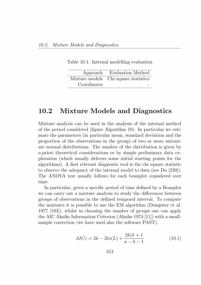
10.2. Mixture Models and Diagnostics
Table 10.1: Internal modelling evaluation
Approach Evaluation MethodMixture models Chi square statistics
Coordinates -
10.2 Mixture Models and Diagnostics
Mixture analysis can be used in the analysis of the internal methodof the period considered (figure Algorithm 19). In particular we esti-mate the parameters (in particular mean, standard deviation and theproportion of the observations in the group) of two or more univari-ate normal distributions. The number of the distribution is given bya-priori theoretical considerations or by simple preliminary data ex-ploration (which usually delivers some initial starting points for thealgorithms). A first relevant diagnostic tool is the chi square statisticto observe the adequacy of the internal model to data (see Du [239]).The ANOVA test usually follows for each beanplot considered overtime.
In particular, given a specific period of time defined by a Beanplotwe can carry out a mixture analysis to study the differences betweengroups of observations in the defined temporal interval. To computethe mixtures it is possible to use the EM algorithm (Dempster et al.1977 [193]), whilst in choosing the number of groups one can applythe AIC Akaike Information Criterion (Akaike 1974 [11]) with a small-sample correction (we have used also the software PAST).
AICc = 2k − 2ln(L) +2k(k + 1
n− k − 1(10.1)
313
Beanplots Model Evaluation
Here k is the number of the parameters, n is the number of dataand L is the likelihood of the model. The lower the AIC, the betterthe number of mixtures that avoid the overfitting and produce thebest fit 1. This procedure compares the number of groups consideredwith the analysis and choosing of the optimal. So we need to comparethe mean and the standard deviation for each group and minimize theAIC in the parameterization.
Each observation can be assigned to each group considering themaximum likelihood approach (see Hammer 2011 [335]). Various meth-ods can be used in this respect as a non-hierarchical clustering method.The usefulness of the method in the diagnostic of the models is thatdata with poor performance with respect to one group or another oneusually calls for a different coefficients estimation or descriptor pointsrepresentation.
10.2.1 Application on real data: Evaluating In-ternal Models: the case of the Mixtures
We consider the Beanplot time series (BTS) for the Dow Jones market1990-2010 (figure 10.1). We estimate the coefficients of the modelusing the mixture approach, so we obtain the coefficients π1, π2, andπ3. At this point we can obtain at the same time the mean of themixtures µ1, µ2 and µ3 that represents another important indicator inthe adequacy of the internal models. We obtain for the first 20 periods(see table 10.2):
1 In the computation the software Past is used: see the Past documentation[758] and Hammer 2011 [335]
314
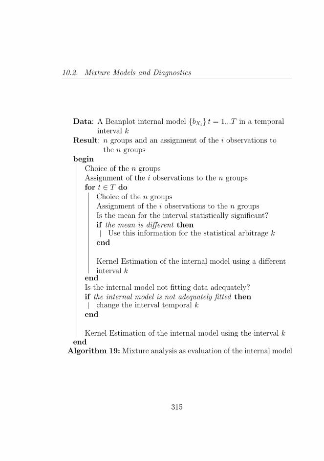
10.2. Mixture Models and Diagnostics
Data: A Beanplot internal model bXt t = 1...T in a temporalinterval k
Result: n groups and an assignment of the i observations tothe n groups
beginChoice of the n groupsAssignment of the i observations to the n groupsfor t ∈ T do
Choice of the n groupsAssignment of the i observations to the n groupsIs the mean for the interval statistically significant?if the mean is different then
Use this information for the statistical arbitrage kend
Kernel Estimation of the internal model using a differentinterval k
endIs the internal model not fitting data adequately?if the internal model is not adequately fitted then
change the interval temporal kend
Kernel Estimation of the internal model using the interval kend
Algorithm 19: Mixture analysis as evaluation of the internal model
315
Beanplots Model Evaluation
10.3 Forecasting Evaluation Methods
It is possible to evaluate the methods used in forecasting2. Here, weanalyse the performances of the forecasting methods by introducingsome measures of adequacy of the performances obtained for the timeseries of attributes. In this sense, we apply these indices of adequacyfor each point computed.
Definition 9. Local Forecast error Et is the difference between theactual value of an attribute time series yt and the predicted value of theattribute time series Ft . Here we denote for the following equations:Et as the prediction error, Ft the value to forecast and n typically thenumber of the observations.
Et = yt − Ft (10.2)
Definition 10. The forecast error for the Beanplot Time Series(BTS) of attribute (BMAE) bXt at t = 1...T is:
BMAEa,t =n∑a=1
(∑nt=1 |Et|n
)(10.3)
Where a is a single attribute of the beanplot. The index is com-puted as the sum of the Local Forecast error Et considering all at-tributes.
At the same time it is possible to compute the Beanplot MeanAbsolute Percentage Error (BMAPE), so we have:
BMAPEa,t =n∑a=1
∑n
t=1
∣∣∣∣EtFt∣∣∣∣
n
(10.4)
2West 2006 [697] Hyndman 2006 [379] Hyndman Koehler (2006) [386]
316
10.3. Forecasting Evaluation Methods
In both cases the objective of using a forecast temporal intervalt = 1...T is to minimize the index. The indexes of adequacy arenot the unique indicators of goodness of fit of an external forecastmodel, in fact, also a poor approximation of the internal models on aspecified benchmark can be a signal of bad approximation of a forecast.Therefore, it is necessary to weight differently the beanplots that arenot fitting well in the real data: an indicator of goodness of fit in theinternal model, given an optimal bandwidth h obtained the BeanplotInternal Model Error for each beanplot b:
BIMEb,t =n∑t=1
h∗t − ht (10.5)
If it is the case that the BIME index is performing in a poor wayit means it is necessary to respecify the external model.
10.3.1 Forecasting evaluation procedure
After having considered the single forecast, the forecast error is thedifference between the real value at time t and the forecast value forthe correspondent period.
A Measure of error (at time t) is:
FE = forecasting error = 100%× |yactual − yforecasting|yactual
(10.6)
for the measures of aggregate error (for more than one period) eachof them has different performances due to the different ways to handleoutliers and observation outside some range. So we use a batteryof indexes to evaluate the forecasting models. Here Et is denotingthe error, yt denotes the series to predict and N is the number ofobservations. So we have:
317
Beanplots Model Evaluation
Mean Absolute Error:
MAE =1
n
n∑t=1
|yt − Ft| =∑n
t=1 |Et|n
(10.7)
Mean Absolute Percentage Error:
MAPE =
∑nt=1 |
Et
yt|
n(10.8)
Symmetric MAPE (see Hyndman 2006 [379]):
sMAPE = mean
(200
|ytFt|(yt + Ft)
)(10.9)
Percent Mean Absolute Deviation:
PMAD =
∑nt=1 |Et|∑nt=1 |yt|
(10.10)
Forecast Skill (related to the MSE)
MSE =
∑nt=1E
2t
n(10.11)
SS = 1− MSE forecast
MSE ref
(10.12)
10.3.2 Discrepancy Measures
Giudici 2006 [312] shows various methods that could be used in thiscase. An important class of methods are related to the Discrepancymeasures, for example, distances on intervals that could be used toevaluate the prediction of the size of the beanplot.
318
10.3. Forecasting Evaluation Methods
10.3.3 Applications on Real data: Evaluating theMixture coefficients estimation and Fore-casting
We consider the data for the Dow Jones Index for the period 1990-2011. We describe here the forecasting procedure:
1. Defining an adequate temporal interval (for example a year)
2. Estimating coefficients of each beanplot in the time series (theπ model coefficients)
3. Obtaining the factorial time series
4. Forecasting the factorial time series (individual forecasts, com-binations, or hybrid models)
5. Diagnostics of the internal and external model
We obtain the forecasting models and we can perform the diagnosticfor each model.
Individual forecasting model on the factorial time series (Auto-ARIMA algorithm)
Forecast combination strategy with model selection. Weight-ing proportional to the forecasting performance of the models: VAR,Setar, Exponential Smoothing, Auto-Arima, Theta, Splinef. Bestmethods: Auto-Arima and Splinef with weights 0.35 and 0.65
10.3.4 Applications on Real data: Evaluating Fore-casting the Dow Jones Index
Dataset 1: Dow Jones dataset 1928-2010. We consider an examplerelated to forecasting the index for the Dow Jones (for the year 2010).
319
Beanplots Model Evaluation
We consider for exploratory purposes the Dow Jones data (1928-10-01–2010-7-30): in total 20,549 observations. Not all the observationsare used to build the models but are considered only in the visualiza-tion of the entire beanplot time series (BTS). We consider as Forecast-ing model period (1998-08-03–2008-08-03) so we define a first set ofrelevant observations in Forecasting. The objective is the Forecastingof the year 2009 and for the interval 2009–2010. Forecasting methodsused: VAR, Auto-Arima, Exponential Smoothing, Smoothing Splines.At the same time as considering Forecasting combinations (Mean, Ex-ponential Smoothing, Auto-Arima) we compare the forecasts obtainedwith whose obtained by the naive model. At that point we considerdifferent diagnostic measures for the models considered. The resultsin the table appear to be good and seem to suggest the use of forecastcombinations in order to improve the results (see table 10.3 and table10.4).
10.4 Clustering Evaluation Methods
At the same time as evaluating the Internal Models it is also possibleto evaluate the External Models as Clustering and Forecasting meth-ods. Typically the internal models can be evaluted by observing theadequacy of the beanplot model data. Here we start with the analysisof the Clustering Methods for the evaluation of the Clusters obtained.For a review of the clustering evaluation methods see Wagner andWagner 2006 [685] and Meila M. 2003 [501].
10.4.1 Internal Criteria of cluster quality
An internal criterion can be based on the idea that a cluster thatminimizes the distance within different clusters is better than one thatmaximizes the distance. It is an internal criteria, one based on the
320
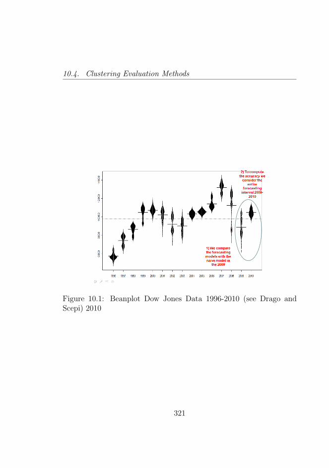
10.4. Clustering Evaluation Methods
Figure 10.1: Beanplot Dow Jones Data 1996-2010 (see Drago andScepi) 2010
321
Beanplots Model Evaluation
results of a specific dataset and not on external information. In thatsense we can consider some indices of adequacy like the Davies Bouldinand the Dunn Index . The best known are the work by Davies Bouldin1979 [168] defined the Davies Bouldin Index (DBI):
DBI =1
n
n∑i=1
maxi 6=k
(µi + µkd(cei, cek)
)(10.13)
In this respect n is the number of clusters obtained by the proce-dure, cx is the centroid of cluster obtained x where µx is the averagedistance of all elements in cluster x to the centroid cex and d(cei, cek)is the distance between the centroids.
And at the same time, the Dunn Index, by Dunn 1974 [242] can bedefined:
DI = min1≤i≤n
min
1≤k≤n,i 6=k
d(i, k)
max1≤j≤n d(j)
(10.14)
where d(i, k) is actually measuring the distance between two genericclusters i and k. The intra-cluster distance in the cluster j, betweenany pair of elements is represented by d(j), by using for example themaximal distance.
The inter-cluster distance d(i, k) between two clusters can be rep-resented also by any type of distance, for example a distance betweenthe centroids of the clusters can be used.
Both these indexes aim to show the adequacy of the cluster analy-sis performed. It is clearly desirable that procedures perform with thelowest Davies Bouldin Index and the maximum Dunn Index possible.This result is expected for the reason that it is better that a clusteringprocess generates clusters with high intra-cluster similarity betweenthe components of each groups and low inter-cluster similarity.
322
10.4. Clustering Evaluation Methods
10.4.2 External Criteria of cluster quality
In this case we consider external evaluation criteria (for example, ex-pert evaluations), so the clustering process is evaluated by consideringthese criteria as the benchmark. Some examples of these indexes arethe Rand and the Jaccard Index. The Rand Index, Rand 1971 [575]:
RI =TPV + TNG
TPV + FPV + FNN + TNG(10.15)
In this case TPV and TNG represent the true answers: respectivelypositives and negatives. In the denominator, the sum of the total ofcases where FPV is the number of false answer positives and theFNN is the number of false answer negatives.
The Jaccard Index, Jaccard 1901 [400] can be defined as the numberof unique elements common to both sets (S1 and S2) also defined asthe size of the intersection of the sets divided by the total number ofunique elements in both sets (or the union). So we have:
J(S1, S2) =|S1 ∩ S2||S1 ∪ S2|
(10.16)
At the same time the Fowlkes Mallows Index, by Fowlkes Mallows1983 [273]
Fa,b =N1,1√
(N1,1 +N0,1)(N1,1 +N1,0)(10.17)
Where in the numerator appear the elements in the same clustera and b set, and in the denominator the sum between the same casesand the others.
323
Beanplots Model Evaluation
10.4.3 Computational Criteria
A criteria to evaluate the cluster quality is also proposed by Suzukiand Shimodaira 2004 [649], Shimodaira 2004 [628] and Shimodaira2002 [627] which proposes an algorithm to assess the uncertainty inhierarchical cluster analysis.
In practice the P-Values of each partition are computed by boot-strap so every cluster can be evaluated. In our sense we can evaluateevery cluster as an external model.
10.5 Forward Search Approaches in Model
Evaluation
The Forward Search (see Atkinson Riani Cerioli 2004 [47], AtkinsonRiani 2004 [46] and Riani 2004 [582] ) Approach can be used to analysethe presence of outliers in the internal models but also in the externalmodels.
In particular in the external models, the methods are applied di-rectly on to the trajectories related to the coefficients estimation andthe descriptor points
In this approach, the observations as outliers are detected, but alsostructural changes over time are detected so it is possible to operateto a respecification of the models.
Rolling approaches can be useful in detecting the different datastructures that could be found in data, so detecting structural changesover time.
324
10.6. The Internal and the External Model Respecification
10.6 The Internal and the External Model
Respecification
If the model is not adequate, then it can be respecified either by con-sidering the outliers found or the different periods shown in the data(for example different structural changes).
Various respecification strategies can be adopted. The outliers canbe imputed, respecified or not considered in a comparative approachwith the initial data. A different approach is that of considering dif-ferent specifications for the internal models, such as different temporalintervals, different bandwidths or different Kernels.
At the same time different respecifications can be adopted for theexternal models, like different periods for building external models (orthe forecasting models), different methods for forecasting the attributetime series or the trajectories generated by the coefficient estimationsand the descriptor points.
The process ends when there can be some satisfaction in the mod-elling and in the clustering or forecasting process. By citing Box andDraper’s work: ”essentially, all models are wrong, but some are useful”(Box and Draper 1987 [98]).
10.6.1 Application on real data: Model Diagnos-tics and Respecification
We start by using as a univariate forecasting model the SmoothingSplines for the three XC attribute time series. Results are comparedwith the real value, where the previous observations represent thenaive forecasting model. We outperform the naive model. In particu-lar we perform an error of 5-6 with respect to the real value (MAPE5-6). The result seems to be good. In the case of the lower part ofthe beanplots (the lower risk interval) this could be considered more
325
Beanplots Model Evaluation
difficult to predict in conditions of high volatility and market crisis.So we expect in these cases a lower performance in the predictionmodels. By considering an alternative and competitive forecastingunivariate model (by Automatic Arima: see Hyndman 2008 [382]) weoutperform the naive forecasting model but we also outperform thesmoothing splines approach. In particular the Automatic Arima algo-rithm selects the best Arima model by minimizing the AIC (AkaikeInformation Criteria index). So in this case the best models tend tooutperform the previous ones we have considered. Here we considerthe Y C attribute time series associated to the XC attribute time se-ries in the stationary framework as an example of the VAR forecastingmodel. Here as well, we outperform the naive model, but the resultsare not as good as in the X case. In fact the Y contains all the com-plexity in our data and so the predictions are therefore necessarily lessaccurate (MAPE around 20). Here for predicting the Y attribute timeseries we use the Smoothing Splines approach in which we are specif-ically trying to denoise the dynamics of the shape. Two times outof three the model outperforms the naive method. The performancesof the methods for the Y are not as good as the X case (and thatcould be expected given the nature of the attribute time series). TheSmoothing Splines approach seems for the Y case the best approachin the forecasting of the Y attribute time series. Here we use thesmoothing splines of the previous example while considering anotherrelevant element: an original algorithm that optimizes the forecastingmodel by selecting the relevant temporal information (by minimizingthe MAPE in the validation period of the model). So the procedureis divided into two distinct parts: running the algorithm to minimizethe MAPE in the validation period and using the interval temporal forthe forecasting. In that way we are explicitly selecting all the relevantset of information (without structural breaks) in our data. The resultsseem to be good (at least in respect to the other models used as bench-mark). The decision to deal with a selection algorithm of the optimal
326
10.6. The Internal and the External Model Respecification
interval for the Y attribute time series can be explained by saying thatwe are dealing with a very volatile attribute time series (the Y ) andwith dynamics with frequently occurring structural changes. So weneed to consider the relevant information in order to try to minimizethe noise that could lead us to not correctly understand their dynam-ics.
See table 1 to compare the different MAPE for the Y as differentattribute time series. The final conclusion of the application is that itis necessary to take into account the Search algorithm to find the bestmodel before attempting a respecification of the models (for exampleby considering a different bandwidth).
327
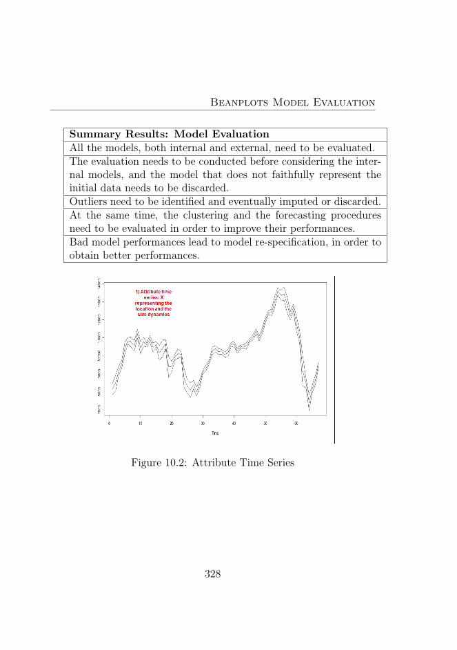
Beanplots Model Evaluation
Summary Results: Model EvaluationAll the models, both internal and external, need to be evaluated.The evaluation needs to be conducted before considering the inter-nal models, and the model that does not faithfully represent theinitial data needs to be discarded.Outliers need to be identified and eventually imputed or discarded.At the same time, the clustering and the forecasting proceduresneed to be evaluated in order to improve their performances.Bad model performances lead to model re-specification, in order toobtain better performances.
Figure 10.2: Attribute Time Series
328

10.6. The Internal and the External Model Respecification
Table 10.2: Internal modelling diagnostics
Model π1 π2 π3 µ1 µ2 µ3 chisq1 0.35 0.32 0.33 247.07 274.69 282.18 0.002 0.00 0.49 0.51 305.60 320.73 321.72 28.313 0.33 0.33 0.34 194.60 243.21 272.96 0.004 0.32 0.32 0.36 101.39 140.45 174.19 0.005 0.34 0.36 0.30 52.38 64.32 76.48 0.006 0.34 0.33 0.33 61.09 95.30 97.25 0.007 0.44 0.20 0.36 94.02 95.81 104.03 0.008 0.32 0.36 0.32 103.38 119.83 139.63 0.009 0.23 0.48 0.29 152.08 158.47 176.96 0.00
10 0.28 0.40 0.31 132.62 178.01 189.61 0.0011 0.46 0.16 0.38 120.50 127.89 147.53 0.0012 0.36 0.29 0.35 136.04 140.59 150.76 0.0013 0.08 0.68 0.24 123.72 131.90 147.30 0.0014 0.33 0.34 0.33 119.78 123.19 123.19 29.5915 0.00 0.70 0.30 104.33 104.92 112.52 10.8316 0.11 0.52 0.38 124.12 134.32 139.72 0.0017 0.36 0.16 0.48 137.56 144.99 147.53 0.0018 0.33 0.35 0.33 157.09 165.68 186.34 0.0019 0.35 0.30 0.34 171.54 200.25 204.34 0.0020 0.32 0.33 0.35 176.28 176.28 180.04 7.65
329
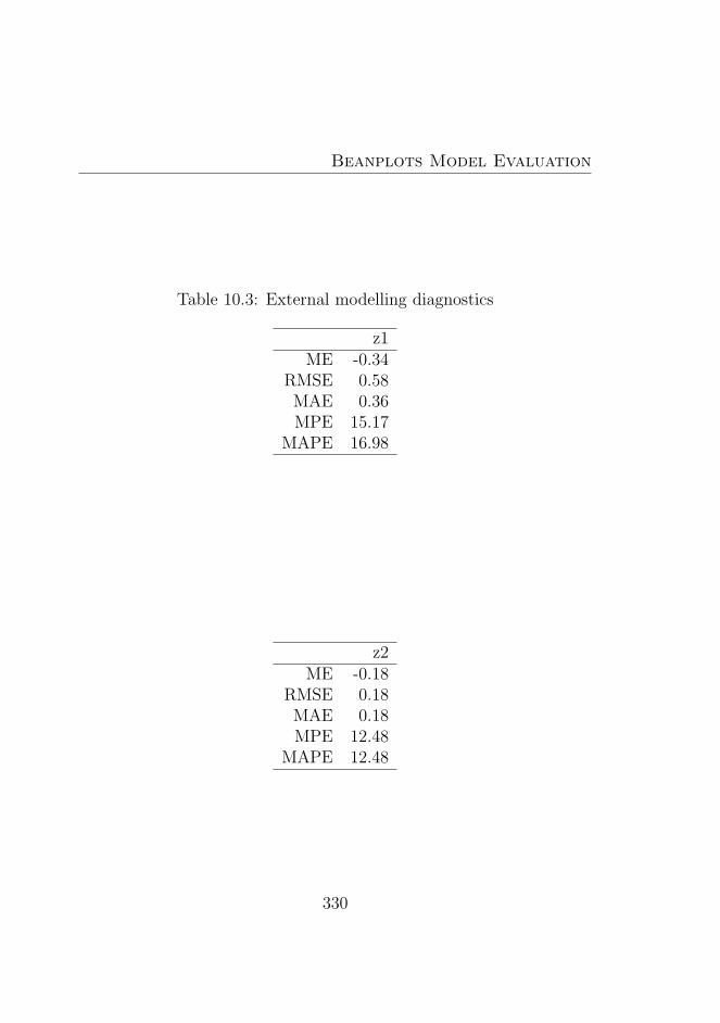
Beanplots Model Evaluation
Table 10.3: External modelling diagnostics
z1ME -0.34
RMSE 0.58MAE 0.36MPE 15.17
MAPE 16.98
z2ME -0.18
RMSE 0.18MAE 0.18MPE 12.48
MAPE 12.48
330
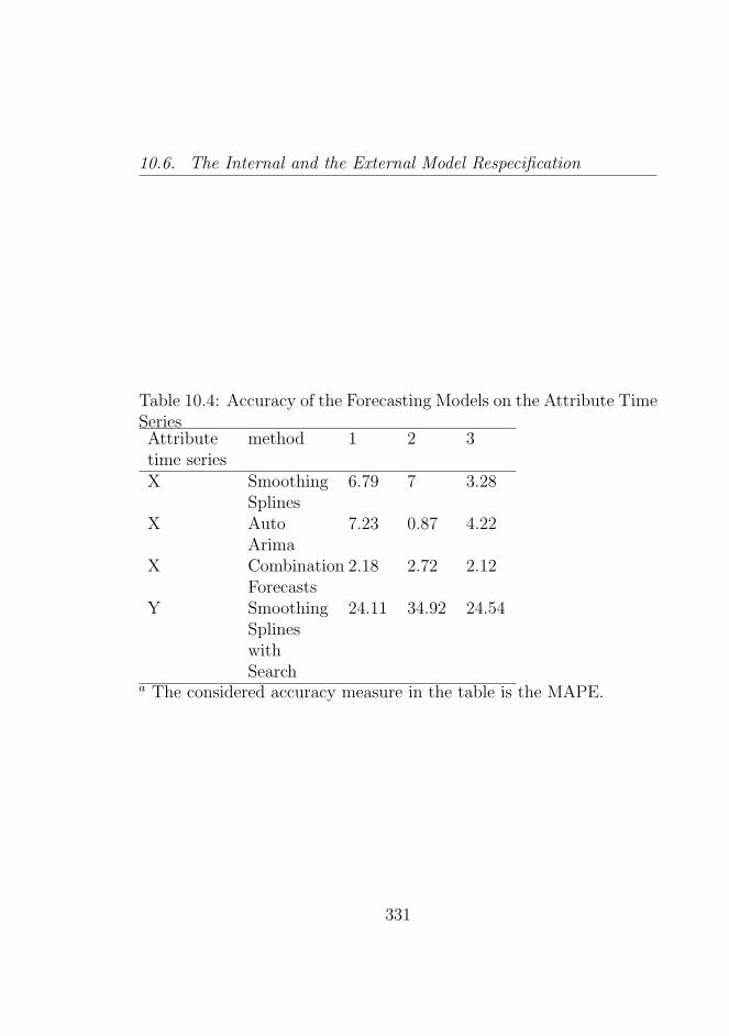
10.6. The Internal and the External Model Respecification
Table 10.4: Accuracy of the Forecasting Models on the Attribute TimeSeriesAttributetime series
method 1 2 3
X SmoothingSplines
6.79 7 3.28
X AutoArima
7.23 0.87 4.22
X CombinationForecasts
2.18 2.72 2.12
Y SmoothingSplineswithSearch
24.11 34.92 24.54
a The considered accuracy measure in the table is the MAPE.
331


Chapter 11
Case Studies: MarketMonitoring, AssetAllocation, StatisticalArbitrage and RiskManagement
The aim of this final chapter is to show the methods seen in the pre-vious chapters in real contexts of Finance application: Market Moni-toring, Asset Allocation, Statistical Arbitrage and Risk Management.Here, an application on real time data is presented.
A second aim of this part is to show the way in which the proposedmethods could improve both the classical methods based on aggre-gate representation (say, intervals, boxplots or histograms) and scalardata. An important characteristic of these data is that they are in realtime, so the data are collected until 26/9/2011, but the models can beupdated because these data are coming from different world markets,day by day. They are Indexes so they represent the compared behavior
Case Studies: Market Monitoring, Asset Allocation,Statistical Arbitrage and Risk Management
of the world markets over time. We present some applications of themethods presented in the thesis based on real data.
11.1 Market Monitoring
Here the objective is to consider, in real time, the market changes formany different stocks by considering the beanplot time series (BTS)compared to the other types of representation. In this respect, visual-ization techniques are very useful and important in order to identifyrapid market phases and effects caused by market shocks such as finan-cial market news, new regulations, etc. From the visualization of thebeanplots it is possible to consider clustering methods or forecastingmethods to make better decisions on market operations (for example,related to risk profiles).
The original dataset of scalar data can be represented as follows.The dates are from 1/1/1990 to 26/9/2011 (figure 11.1) and they comefrom Yahoo Finance, in which we select the time series related to theclosing prices of the most important world stockmarket indexes (DowJones or DJI, Dax, Cac 40 etc.). In all these cases the interestingpoint is that we do not observe the different time series due to thedifferent scales and the data quantity. We need to consider some al-ternative representations (for example: intervals, boxplots, histogramsor beanplots) for a better data visualization and exploration.
The visualization of the time series is in figure 11.2 and figure 11.3.By considering the original time series we can observe the differentscales. It is clear in this case that visualization is very difficult andwe cannot observe the details by considering each time series. At thesame time we could be interested in considering some specific intervals(temporal intervals) to analyse the intra-period variation. This type ofanalysis could be very interesting in comparing the risk profiles of thetime series. By considering the Scalar time series we can observe the
334
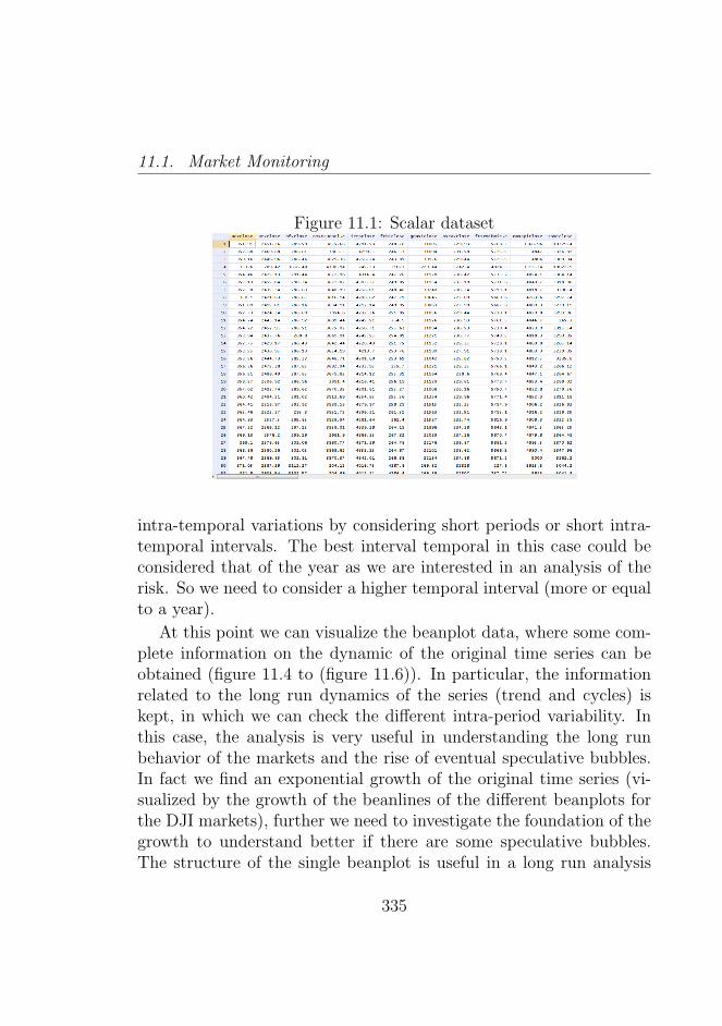
11.1. Market Monitoring
Figure 11.1: Scalar dataset
intra-temporal variations by considering short periods or short intra-temporal intervals. The best interval temporal in this case could beconsidered that of the year as we are interested in an analysis of therisk. So we need to consider a higher temporal interval (more or equalto a year).
At this point we can visualize the beanplot data, where some com-plete information on the dynamic of the original time series can beobtained (figure 11.4 to (figure 11.6)). In particular, the informationrelated to the long run dynamics of the series (trend and cycles) iskept, in which we can check the different intra-period variability. Inthis case, the analysis is very useful in understanding the long runbehavior of the markets and the rise of eventual speculative bubbles.In fact we find an exponential growth of the original time series (vi-sualized by the growth of the beanlines of the different beanplots forthe DJI markets), further we need to investigate the foundation of thegrowth to understand better if there are some speculative bubbles.The structure of the single beanplot is useful in a long run analysis
335
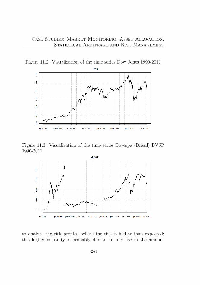
Case Studies: Market Monitoring, Asset Allocation,Statistical Arbitrage and Risk Management
Figure 11.2: Visualization of the time series Dow Jones 1990-2011
Figure 11.3: Visualization of the time series Bovespa (Brazil) BVSP1990-2011
to analyze the risk profiles, where the size is higher than expected;this higher volatility is probably due to an increase in the amount
336
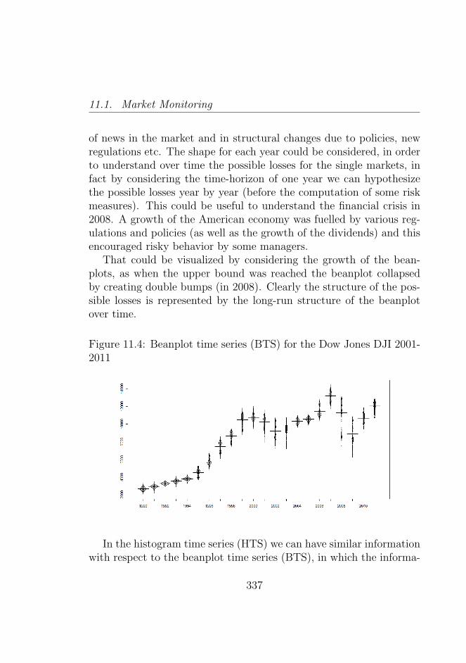
11.1. Market Monitoring
of news in the market and in structural changes due to policies, newregulations etc. The shape for each year could be considered, in orderto understand over time the possible losses for the single markets, infact by considering the time-horizon of one year we can hypothesizethe possible losses year by year (before the computation of some riskmeasures). This could be useful to understand the financial crisis in2008. A growth of the American economy was fuelled by various reg-ulations and policies (as well as the growth of the dividends) and thisencouraged risky behavior by some managers.
That could be visualized by considering the growth of the bean-plots, as when the upper bound was reached the beanplot collapsedby creating double bumps (in 2008). Clearly the structure of the pos-sible losses is represented by the long-run structure of the beanplotover time.
Figure 11.4: Beanplot time series (BTS) for the Dow Jones DJI 2001-2011
In the histogram time series (HTS) we can have similar informationwith respect to the beanplot time series (BTS), in which the informa-
337
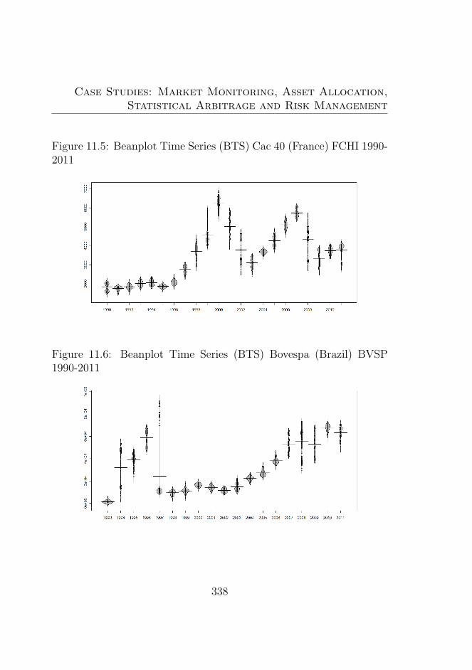
Case Studies: Market Monitoring, Asset Allocation,Statistical Arbitrage and Risk Management
Figure 11.5: Beanplot Time Series (BTS) Cac 40 (France) FCHI 1990-2011
Figure 11.6: Beanplot Time Series (BTS) Bovespa (Brazil) BVSP1990-2011
338

11.1. Market Monitoring
tion is more dependent on the number of bins chosen and this usuallyconstraints the original data (figure 11.7). Various possible interpre-tations of the beanplots can be repeated also for the histogram timeseries (HTS).
Figure 11.7: Histogram Time Series (HTS) Dow Jones DJI 1990-2011
The Interval time series (ITS) shows the upper and the lower boundand the entity of the possible losses over the time. The problem forthe intervals could be that we are not able to understand the differencebetween eventual outliers in our data. Intervals can show, as in thecase of the beanplots, the risk profiles (the possible losses) in whichan extreme event is represented, for example a market crash. Clearlythe usefulness of the interval time series (ITS) is in the fact that itis possible to define the lower and the upper bounds in the temporalintervals. In that sense it could be useful to consider lower and upperbound in the temporal intervals, by taking into account the lower andthe upper interval of variations over the time (figure 11.10).
The Boxplot time series (BoTS) tend to show a smoothed image ofthe intra-temporal variation over the time (figure 11.13). It is possible
339
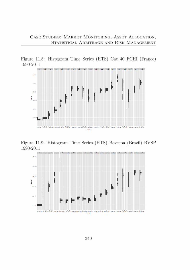
Case Studies: Market Monitoring, Asset Allocation,Statistical Arbitrage and Risk Management
Figure 11.8: Histogram Time Series (HTS) Cac 40 FCHI (France)1990-2011
Figure 11.9: Histogram Time Series (HTS) Bovespa (Brazil) BVSP1990-2011
340
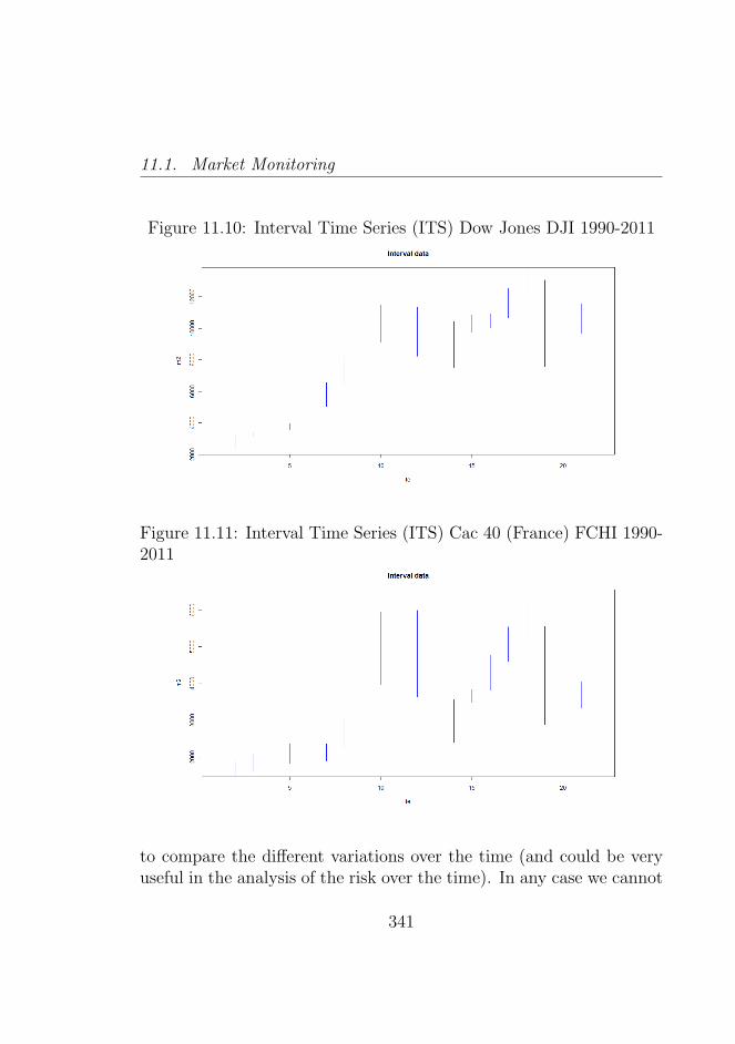
11.1. Market Monitoring
Figure 11.10: Interval Time Series (ITS) Dow Jones DJI 1990-2011
Figure 11.11: Interval Time Series (ITS) Cac 40 (France) FCHI 1990-2011
to compare the different variations over the time (and could be veryuseful in the analysis of the risk over the time). In any case we cannot
341
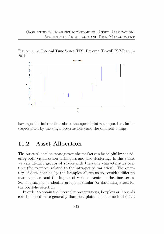
Case Studies: Market Monitoring, Asset Allocation,Statistical Arbitrage and Risk Management
Figure 11.12: Interval Time Series (ITS) Bovespa (Brazil) BVSP 1990-2011
have specific information about the specific intra-temporal variation(represented by the single observations) and the different bumps.
11.2 Asset Allocation
The Asset Allocation strategies on the market can be helpful by consid-ering both visualization techniques and also clustering. In this sense,we can identify groups of stocks with the same characteristics overtime (for example, related to the intra-period variation). The quan-tity of data handled by the beanplot allows us to consider differentmarket phases and the impact of various events on the time series.So, it is simpler to identify groups of similar (or dissimilar) stock forthe portfolio selection.
In order to obtain the internal representations, boxplots or intervalscould be used more generally than beanplots. This is due to the fact
342
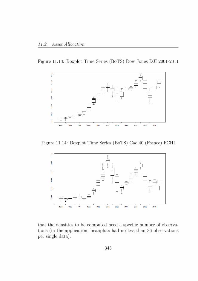
11.2. Asset Allocation
Figure 11.13: Boxplot Time Series (BoTS) Dow Jones DJI 2001-2011
Figure 11.14: Boxplot Time Series (BoTS) Cac 40 (France) FCHI
that the densities to be computed need a specific number of observa-tions (in the application, beanplots had no less than 36 observationsper single data).
343
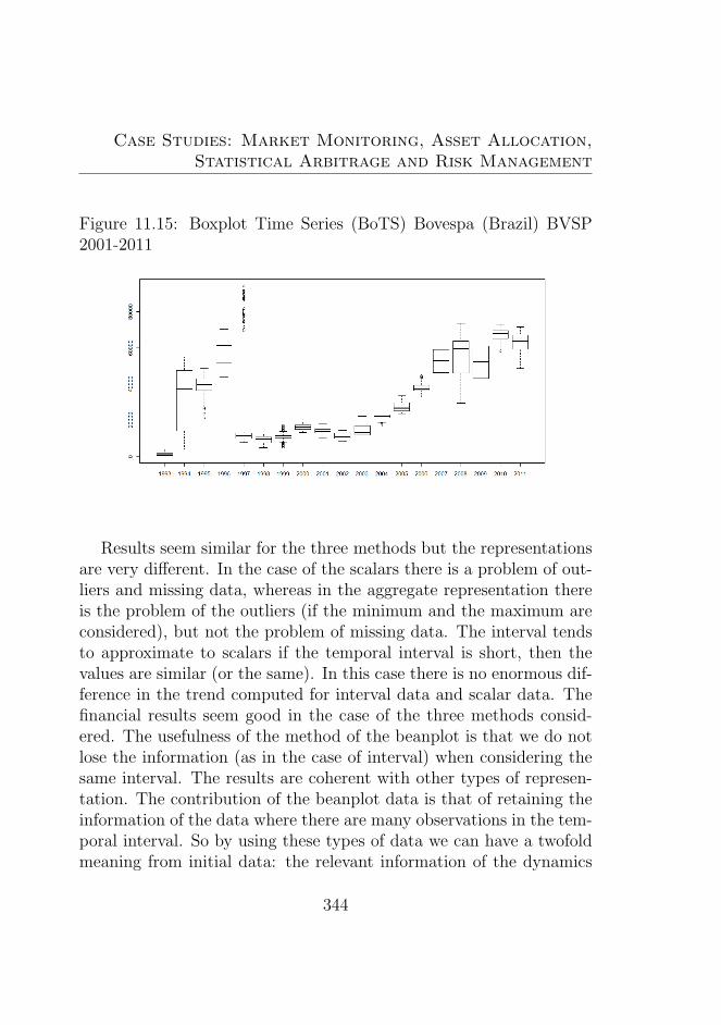
Case Studies: Market Monitoring, Asset Allocation,Statistical Arbitrage and Risk Management
Figure 11.15: Boxplot Time Series (BoTS) Bovespa (Brazil) BVSP2001-2011
Results seem similar for the three methods but the representationsare very different. In the case of the scalars there is a problem of out-liers and missing data, whereas in the aggregate representation thereis the problem of the outliers (if the minimum and the maximum areconsidered), but not the problem of missing data. The interval tendsto approximate to scalars if the temporal interval is short, then thevalues are similar (or the same). In this case there is no enormous dif-ference in the trend computed for interval data and scalar data. Thefinancial results seem good in the case of the three methods consid-ered. The usefulness of the method of the beanplot is that we do notlose the information (as in the case of interval) when considering thesame interval. The results are coherent with other types of represen-tation. The contribution of the beanplot data is that of retaining theinformation of the data where there are many observations in the tem-poral interval. So by using these types of data we can have a twofoldmeaning from initial data: the relevant information of the dynamics
344
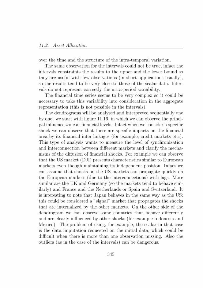
11.2. Asset Allocation
over the time and the structure of the intra-temporal variation.The same observation for the intervals could not be true, infact the
intervals constraints the results to the upper and the lower bound sothey are useful with few observations (in short applications usually),so the results tend to be very close to those of the scalar data. Inter-vals do not represent correctly the intra-period variability.
The financial time series seems to be very complex so it could benecessary to take this variability into consideration in the aggregaterepresentation (this is not possible in the intervals).
The dendrograms will be analysed and interpreted sequentially oneby one: we start with figure 11.16, in which we can observe the princi-pal influence zone at financial levels. Infact when we consider a specificshock we can observe that there are specific impacts on the financialarea by its financial inter-linkages (for example, credit markets etc.).This type of analysis wants to measure the level of synchronizationand interconnection between different markets and clarify the mecha-nisms of the diffusion of financial shocks. For example we can observethat the US market (DJI) presents characteristics similar to Europeanmarkets even though maintaining its independent position. Infact wecan assume that shocks on the US markets can propagate quickly onthe European markets (due to the interconnections) with lags. Moresimilar are the UK and Germany (so the markets tend to behave sim-ilarly) and France and the Netherlands or Spain and Switzerland. Itis interesting to note that Japan behaves in the same way as the US:this could be considered a ”signal” market that propagates the shocksthat are internalized by the other markets. On the other side of thedendrogram we can observe some countries that behave differentlyand are clearly influenced by other shocks (for example Indonesia andMexico). The problem of using, for example, the scalar in that caseis the data imputation requested on the initial data, which could bedifficult when there is more than one observation missing. Also theoutliers (as in the case of the intervals) can be dangerous.
345
Case Studies: Market Monitoring, Asset Allocation,Statistical Arbitrage and Risk Management
By considering the intervals in a short period the results do notappear to change using the center. So results seem to be consistentwith the case of the scalars in which we avoid the problem of missingdata, and the problem of outliers (in this case we need to use somedifferent intervals that exclude outliers, for example trimmed means,etc.). In the case of the year temporal interval the results seem to beconsistent with previous results, in which we can observe some shortdifferences on the dendrograms.
By considering the Beanplot time series (BTS) and repeating theanalysis above, it is interesting to note that we observe similar infor-mation for the factor F1, obtained as the synthesis of the attributetime series related to the size and the location of the beanplot timeseries (BTS). The F1 (see figure 11.18 and the associated dissimilar-ity matrix obtained in figure 11.17) shows similar information withrespect to the scalar and the interval case. In this case the defini-tion of the influence areas seems more precise. In fact there are somedifferences, for example Spain and Switzerland tend to behave differ-ently with respect to the shocks. Other situations seem to be clearer:Hong Kong is very similar to Singapore, and the Japan and the USmarket seem to behave as ”signal markets” with respect to other mar-kets. Austria is clearly an outlier, probably due to the market sizeand its microstructural characteristics. Considering the second factor(figure 11.23), which is more related to the shape characteristics of thebeanplot time series (BTS), we can have more information on the fi-nancial interconnections and the exact direction of the shocks on time.In particular, Mexico and Indonesia tend to have some very peculiarresponses to the shocks (in fact they are particular markets charac-terised by very peculiar macroeconomic contexts). In the other partof the dendrograms we can observe the specific short run impacts ofthe shocks (that are related to the shapes of the beanplot time seriesBTS).
The other dendrograms are considered for robustness checks and
346
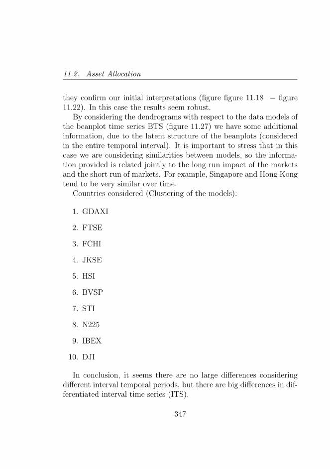
11.2. Asset Allocation
they confirm our initial interpretations (figure figure 11.18 − figure11.22). In this case the results seem robust.
By considering the dendrograms with respect to the data models ofthe beanplot time series BTS (figure 11.27) we have some additionalinformation, due to the latent structure of the beanplots (consideredin the entire temporal interval). It is important to stress that in thiscase we are considering similarities between models, so the informa-tion provided is related jointly to the long run impact of the marketsand the short run of markets. For example, Singapore and Hong Kongtend to be very similar over time.
Countries considered (Clustering of the models):
1. GDAXI
2. FTSE
3. FCHI
4. JKSE
5. HSI
6. BVSP
7. STI
8. N225
9. IBEX
10. DJI
In conclusion, it seems there are no large differences consideringdifferent interval temporal periods, but there are big differences in dif-ferentiated interval time series (ITS).
347
Case Studies: Market Monitoring, Asset Allocation,Statistical Arbitrage and Risk Management
It is possible to observe that the clustering shows series with similardata structures. But the real question is: In what way is it possibleto anticipate crises?
By clustering, using the model distance, we cluster the differentmodels, in which we take into account the latent and the structuralinformation (for each temporal interval). So we can obtain some ex-pected results (as in the case of Hong Kong and Singapore) but alsointeresting results.
Figure 11.16: Clustering original time series (2000-2011)
11.3 Statistical Arbitrage
For Statistical Arbitrage, strategies identifying pairs (or groups) ofstocks showing very similar characteristics over time are fundamental.By identifying some strong correlation between different stocks overtime it is possible to operate and make profits on the divergences inthe trajectories. Thus, the Beanplot, and the related techniques seen
348
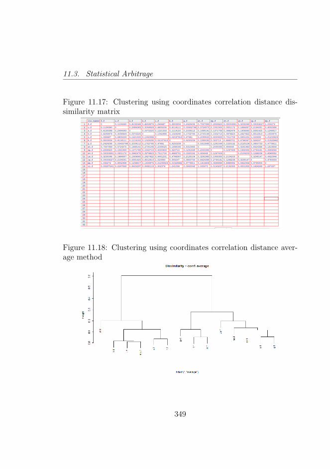
11.3. Statistical Arbitrage
Figure 11.17: Clustering using coordinates correlation distance dis-similarity matrix
Figure 11.18: Clustering using coordinates correlation distance aver-age method
349
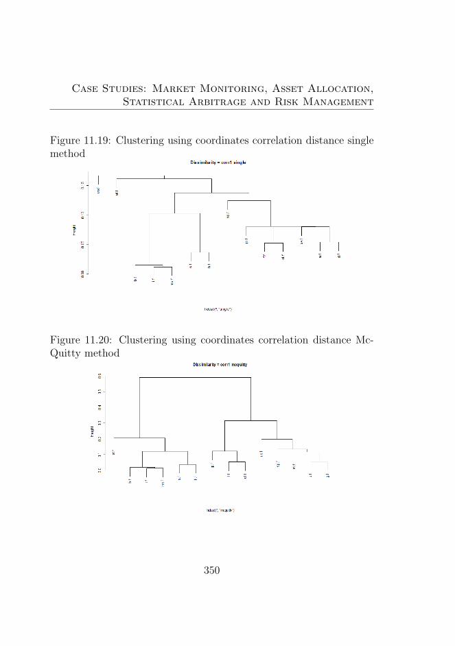
Case Studies: Market Monitoring, Asset Allocation,Statistical Arbitrage and Risk Management
Figure 11.19: Clustering using coordinates correlation distance singlemethod
Figure 11.20: Clustering using coordinates correlation distance Mc-Quitty method
350
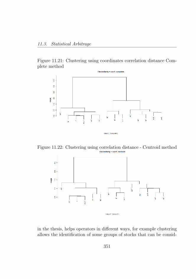
11.3. Statistical Arbitrage
Figure 11.21: Clustering using coordinates correlation distance Com-plete method
Figure 11.22: Clustering using correlation distance - Centroid method
in the thesis, helps operators in different ways, for example clusteringallows the identification of some groups of stocks that can be consid-
351
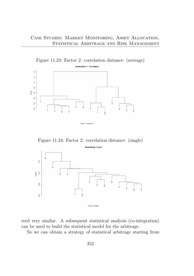
Case Studies: Market Monitoring, Asset Allocation,Statistical Arbitrage and Risk Management
Figure 11.23: Factor 2: correlation distance: (average)
Figure 11.24: Factor 2: correlation distance: (single)
ered very similar. A subsequent statistical analysis (co-integration)can be used to build the statistical model for the arbitrage.
So we can obtain a strategy of statistical arbitrage starting from
352
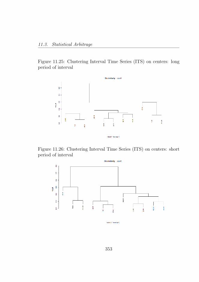
11.3. Statistical Arbitrage
Figure 11.25: Clustering Interval Time Series (ITS) on centers: longperiod of interval
Figure 11.26: Clustering Interval Time Series (ITS) on centers: shortperiod of interval
353
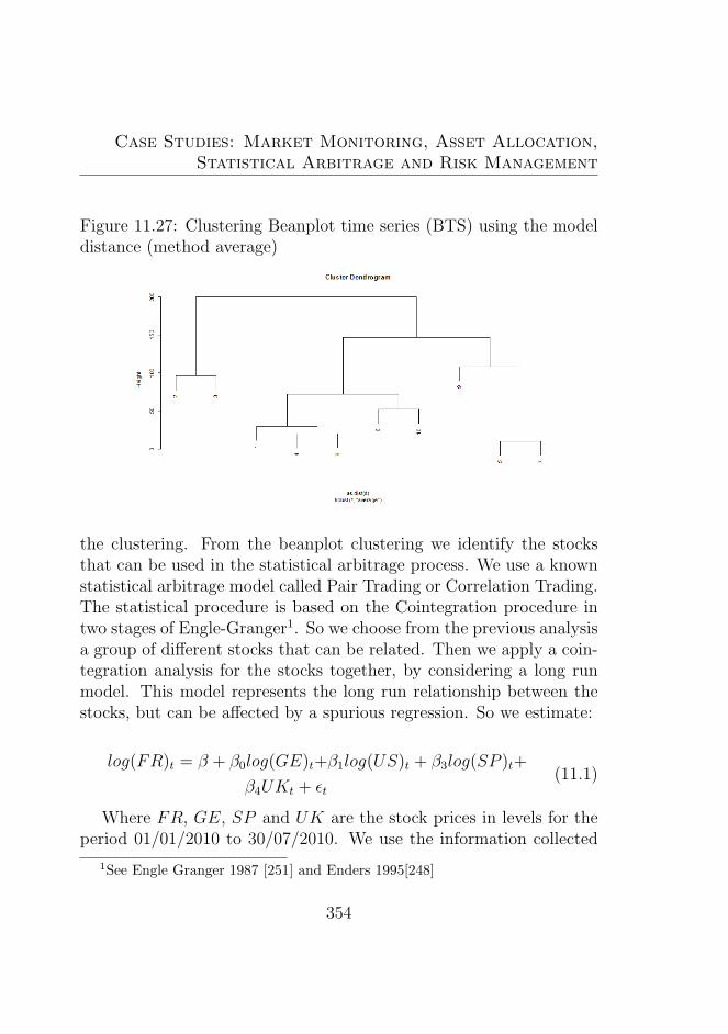
Case Studies: Market Monitoring, Asset Allocation,Statistical Arbitrage and Risk Management
Figure 11.27: Clustering Beanplot time series (BTS) using the modeldistance (method average)
the clustering. From the beanplot clustering we identify the stocksthat can be used in the statistical arbitrage process. We use a knownstatistical arbitrage model called Pair Trading or Correlation Trading.The statistical procedure is based on the Cointegration procedure intwo stages of Engle-Granger1. So we choose from the previous analysisa group of different stocks that can be related. Then we apply a coin-tegration analysis for the stocks together, by considering a long runmodel. This model represents the long run relationship between thestocks, but can be affected by a spurious regression. So we estimate:
log(FR)t = β + β0log(GE)t+β1log(US)t + β3log(SP )t+
β4UKt + εt(11.1)
Where FR, GE, SP and UK are the stock prices in levels for theperiod 01/01/2010 to 30/07/2010. We use the information collected
1See Engle Granger 1987 [251] and Enders 1995[248]
354
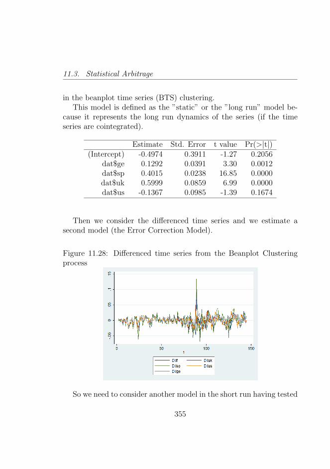
11.3. Statistical Arbitrage
in the beanplot time series (BTS) clustering.This model is defined as the ”static” or the ”long run” model be-
cause it represents the long run dynamics of the series (if the timeseries are cointegrated).
Estimate Std. Error t value Pr(>|t|)(Intercept) -0.4974 0.3911 -1.27 0.2056
dat$ge 0.1292 0.0391 3.30 0.0012dat$sp 0.4015 0.0238 16.85 0.0000dat$uk 0.5999 0.0859 6.99 0.0000dat$us -0.1367 0.0985 -1.39 0.1674
Then we consider the differenced time series and we estimate asecond model (the Error Correction Model).
Figure 11.28: Differenced time series from the Beanplot Clusteringprocess
So we need to consider another model in the short run having tested
355
Case Studies: Market Monitoring, Asset Allocation,Statistical Arbitrage and Risk Management
the cointegration in the model. Thus we can model the differences andthe residual of the long run model.
∆log(FR)t = β+β0∆log(GE)t + β1∆log(US)t+
β3∆log(SP )t + β4∆UKt+zt−1 + εt(11.2)
Where the time series are differenced together and the zt−1 is theresidual from the static model. In this sense we can model the de-viations from the long run equilibrium (the static model). These de-viations can be used for the statistical arbitrage using appropriatestrategies.
Estimate Std. Error t value Pr(>|t|)(Intercept) -0.0000 0.0006 -0.04 0.9649
dat3$ge 0.1115 0.0470 2.37 0.0191dat3$sp 0.6334 0.0314 20.15 0.0000dat3$uk 0.0729 0.0617 1.18 0.2398dat3$us -0.0950 0.0627 -1.51 0.1321
res -0.1641 0.0471 -3.48 0.0007
11.4 Risk Management
Risk Management can benefit in various ways from these techniques.The visualization allows one to understand and compare the differentrisk profiles between stocks, whereas clustering helps in the identifi-cation of similar stocks in some risk profiles. The visualization andthe prototypes can be used to identify early warnings for potentialcrises or financial problems. Using the Beanplot time series (BTS) itis possible to forecast the future levels of risk and losses over time.
356
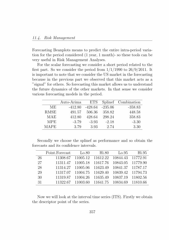
11.4. Risk Management
Forecasting Beanplots means to predict the entire intra-period varia-tion for the period considered (1 year, 1 month)- so these tools can bevery useful in Risk Management Analyses.
For the scalar forecasting we consider a short period related to thefirst part. So we consider the period from 1/1/1990 to 26/9/2011. Itis important to note that we consider the US market in the forecastingbecause in the previous part we observed that this market acts as a”signal” for others. So forecasting this market allows us to understandthe future dynamics of the other markets. In that sense we considervarious forecasting models in the period.
Auto-Arima ETS Splinef CombinationME -412.80 -428.64 -235.06 -358.83
RMSE 491.57 506.36 358.82 448.58MAE 412.80 428.64 298.24 358.83MPE -3.79 -3.93 -2.18 -3.30
MAPE 3.79 3.93 2.74 3.30
Secondly we choose the splinef as performance and so obtain theforecasts and its confidence intervals.
Point.Forecast Lo.80 Hi.80 Lo.95 Hi.9526 11308.67 11005.12 11612.22 10844.43 11772.9127 11311.47 11005.18 11617.76 10843.05 11779.9028 11314.27 11005.06 11623.49 10841.37 11787.1729 11317.07 11004.75 11629.40 10839.42 11794.7330 11319.87 11004.26 11635.49 10837.19 11802.5631 11322.67 11003.60 11641.75 10834.69 11810.66
Now we will look at the interval time series (ITS). Firstly we obtainthe descriptor point of the series.
357
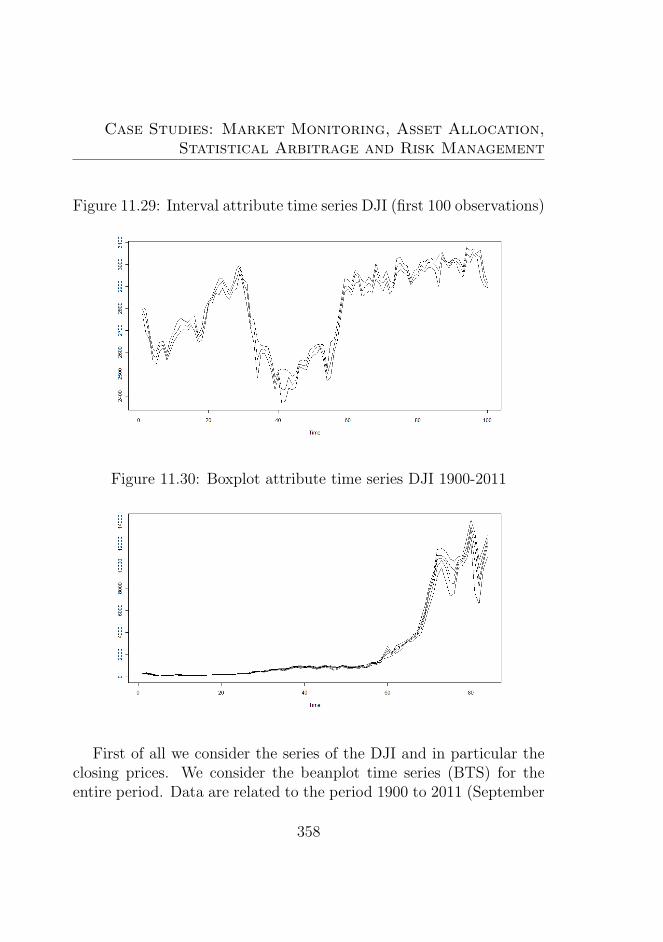
Case Studies: Market Monitoring, Asset Allocation,Statistical Arbitrage and Risk Management
Figure 11.29: Interval attribute time series DJI (first 100 observations)
Figure 11.30: Boxplot attribute time series DJI 1900-2011
First of all we consider the series of the DJI and in particular theclosing prices. We consider the beanplot time series (BTS) for theentire period. Data are related to the period 1900 to 2011 (September
358
11.4. Risk Management
2011). The first representation we choose uses coordinates. As usualwe choose a bandwidth for the entire time series and we forecast theattribute time series for the beanplot time series (BTS) as well. Weforecast both for the XC and for the Y C . The procedure is dividedinto three steps:
1. Forecasting the attribute time series using competitive methods
2. Forecasting the attribute time series using forecasts combina-tions (by an appropriate weighting scheme)
3. Detecting the best set of information using the Search Algorithm(for the Y C)
On the XC Forecasting we use the methods Auto-Arima and Ets(h=3). The result is particularly good for forecasting on the shorttime. If we obtain a general MAPE on 1-5 means then it signifies wecan predict well the locations and the size of the beanplot over time.
On the XC Forecasting using combinations (h=5) it is interestingto note that by using combinations we can use a higher horizon forthe forecasting process. The MAPE in that sense is higher than inthe case of the single forecasts (MAPE 7-8) but the horizon chosen ishigher.
Using a Search Algorithm (on minima), the forecasting model achievesa MAPE of 1.43 as accuracy.
The aim of the Search algorithm is the identification of the bestinformation set. In practice the analysis is divided into two steps:first, we consider the temporal intervals that minimize the error in theforecasting (for example by minimizing the MAPE), then we use thisset of information in the forecasting process.
We consider the search on the Y C , because of its volatility. Theforecasting process is on h=1, in fact it is necessary to maximize theinformation and the data. In any case the search algorithm is not
359
Case Studies: Market Monitoring, Asset Allocation,Statistical Arbitrage and Risk Management
strictly necessary for the XC forecasting due to the different stabilitylevel of the attribute time series, but it is necessary for the Y C . TheMape for the Minima (MAPE 1.43) is good after the procedure of thesearch algorithm.
A second step could be to Forecast using Mixtures, as we want toforecast the structural part of our beanplots over time.
The Automatic-ARIMA algorithm (and the associated ARIMA model)is the forecasting model we have chosen. By using this model we ob-tain a satisfying diagnostic and the forecasts obtained are (MAPE=5).So we conclude that the model can be used both for the predictionand the simulation.
The factor is well predicted by using only one method. When onemethod is better than others the combination is not so efficient. Us-ing other methods it is abstractly possible to improve the results if theresults of the methods are not able to discriminate the optimal one.The capability of forecasting depends on the quality of the group usedin the combination.
We compare the results with the forecasting of the scalars, the box-plot, and the interval time series (ITS). The results are strictly relatedto the descriptors used and the data considered, so the results can vary.In any case it is important to observe that the focus of each method isvery different: the scalars are a way of forecasting in the short period,so we predict observation by observation (and so we have not a feelabout intra-period variability). In the case of boxplot and intervalwe predict using some relevant descriptors (upper and lower bound,quantiles etc.) where it is important to know that the external modeladequacy depends on the general structure of the model chosen, on thecomplex data and its representation, and that different complex datadeliver different information. In that sense the beanplot time series(BTS) are related usually to information on intra-temporal variation,that is, on more observations than in the case of interval and boxplot.So they are very useful when we need to compare long run dynamics
360
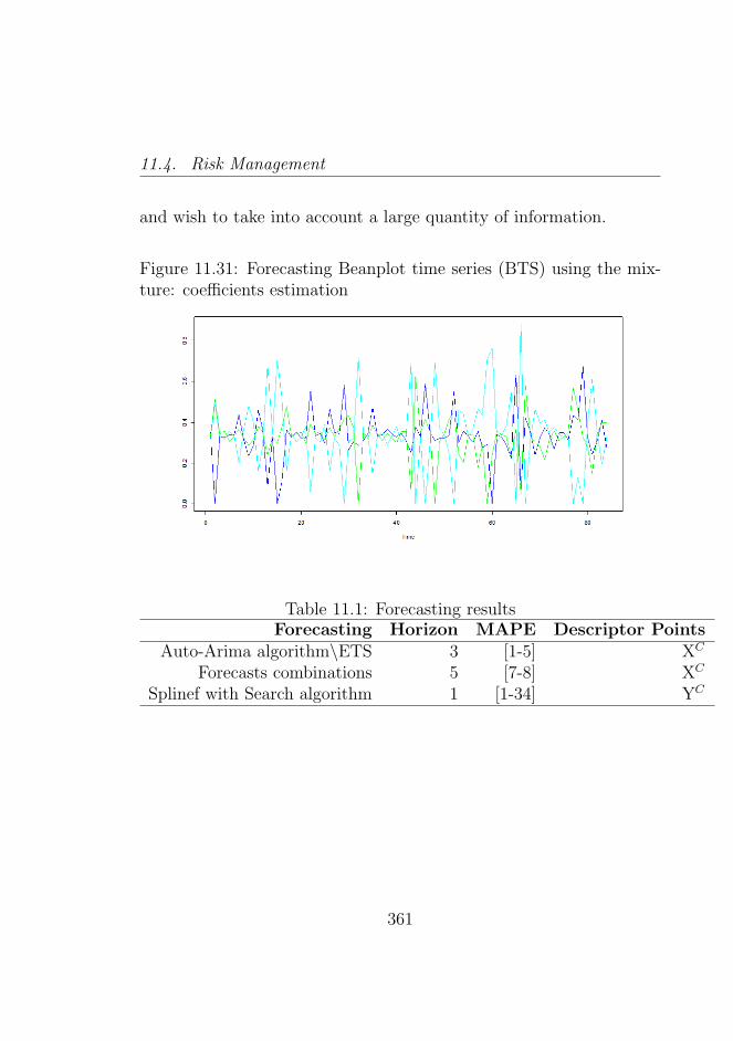
11.4. Risk Management
and wish to take into account a large quantity of information.
Figure 11.31: Forecasting Beanplot time series (BTS) using the mix-ture: coefficients estimation
Table 11.1: Forecasting resultsForecasting Horizon MAPE Descriptor Points
Auto-Arima algorithm\ETS 3 [1-5] XC
Forecasts combinations 5 [7-8] XC
Splinef with Search algorithm 1 [1-34] YC
361
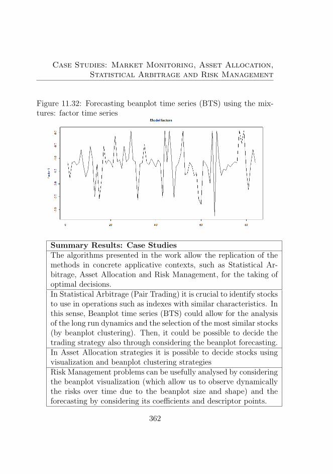
Case Studies: Market Monitoring, Asset Allocation,Statistical Arbitrage and Risk Management
Figure 11.32: Forecasting beanplot time series (BTS) using the mix-tures: factor time series
Summary Results: Case StudiesThe algorithms presented in the work allow the replication of themethods in concrete applicative contexts, such as Statistical Ar-bitrage, Asset Allocation and Risk Management, for the taking ofoptimal decisions.In Statistical Arbitrage (Pair Trading) it is crucial to identify stocksto use in operations such as indexes with similar characteristics. Inthis sense, Beanplot time series (BTS) could allow for the analysisof the long run dynamics and the selection of the most similar stocks(by beanplot clustering). Then, it could be possible to decide thetrading strategy also through considering the beanplot forecasting.In Asset Allocation strategies it is possible to decide stocks usingvisualization and beanplot clustering strategiesRisk Management problems can be usefully analysed by consideringthe beanplot visualization (which allow us to observe dynamicallythe risks over time due to the beanplot size and shape) and theforecasting by considering its coefficients and descriptor points.
362
Conclusions and Extensionsfor Future Research
The world of data is changing. The terms Analytics, Data Products,Data Science are frequent in the business world today. At the sametime, the problem is associated with the ubiquity of huge datasets (bigdata) and the continuous flow of information that can add value to thebusiness. In modern finance, developments are related to the existenceof new types of data like High Frequency Data that can be consideredthe original data type with respect to its aggregate version, and thisleads to a loss of information. In all these contexts the problem is torepresent and to use adequately the information in the data.
In that sense, it is a question of using the data according to a modelto gain an economic advantage on the continuous flow of informationthat the new technologies allow.
So the challenge for the new statisticians or the new profession, thedata scientist, is not only to analyse this flow of data, but at the sametime to gain knowledge and a business value from this information.In this respect, of great relevance is a sequence of well-defined phases:data collection (or data storage), data cleaning, data visualization, andfinally, data analysis (or analytics) for a specific purpose: forecastingand collecting information for making better decisions. However, themain focus of the thesis is on special types of time series, defined as
363
Conclusions
high frequency data. The data are considered to be unequally spaced,to possess an overwhelming number of observations, errors (that callfor special filters), missing observations, price discreteness, seasonali-ties and volatility clustering. These data require specific econometricmethods in their analysis and the data aggregation seems not to beappropriate, due to the fact that information loss occurs.
In this thesis, we innovate this scheme by proposing a new type ofdata. Scalar data are used extensively in the Data Science world, andin the Financial sector. We have shown that these data sometimesrepresent, for example in the context of huge datasets, a difficult pieceof information to use because of the difficulties in visualization (andso, in data exploration). The most frequent solution to that of usingScalar Data is that of using some types of aggregation which howeverresult in information loss. In any case, the problem in High FrequencyData and in general in Huge Data Sets is not a loss information initself but the representation of the underlying information. In fact thesingle scalar is sometimes not an adequate way to represent the data inwhich we want to explore some patterns of intra-data variation. Thistype of information could be very useful in a very important series ofbusiness or financial contexts.
We consider the changing intra-period variability or the data asgenuine representations as intervals, histograms, densities or bean-plots. The intra-period variability (modelled as internal model) of therepresentation is important because we need to consider the pattern ofvariation in the time as the relevant phenomenon. If we consider thedynamics of the phenomenon over time we consider the inter-periodvariability. We model the intra-period variability using external mod-els. The optimal compromise between the two models and the tworepresentations needs to be optimized in the cycle, described in thethesis as visualization, exploration, internal modelling, clustering orforecasting (external modelling) and model evaluation. Non-optimalmodels can be re-specified. The actual literature does not consider
364
Conclusions
the approach to model differently from the intra-period and the inter-period variation, but this seems an important aspect of the presentwork because we capture the structural aspects of the data. This ideais an innovation of the present work. In particular, we are explicitlytaking into account the capability of the data to capture the intra-period variability of the phenomenon (which could be used to extractvalue from data). At the same time the techniques required for theobjectives need to be considered in real time, so throughout the the-sis we consider different tools that use the changing information in areal time ideal context that both identify the relevant information andachieve the updating of the important statistical results over time.
A relevant problem running through the entire thesis is the choiceof the appropriate temporal interval (for example, the choices betweenhour, day, week, month and year). There is no specific answer as towhat is the best temporal interval in every situation. In general, thetemporal interval depends on the specific application. So, in somecases it could be useful to decide a temporal interval related to shortperiods, for example in trading applications, whereas in risk manage-ment it is more important to consider a higher temporal interval (say,a year) to cover all the possible economic phenomena in a temporalrange.
The choice of the best representation is strongly related to thechoice of the best temporal interval. In particular, by choosing thetemporal interval it is possible to select the best representation. There-fore, in each concrete application it is very important to define before-hand a useful temporal interval (day, month, year, etc.) then to choosethe most useful internal representation in order to extract the knowl-edge from the data with the objective of decision making.
So for a specific reason we have worked extensively on original (verylong) time series that could be considered in real time, because all ourapplications follow the evolution of the financial markets. We consideras well the steps of data analysis: not only considering the original time
365
Conclusions
series of the scalar data but also its aggregate representation, this max-imizes the information on variability much more than the interval andthe histogram. Data in this respect are obtained by a Kernel DensityEstimation, in which in the final data (the beanplot data) the com-plete information of the location, the size (the intra-period variability)and the shape (the entire data structure) are represented.
These types of data can be particularly advantageous in the contextof high frequency data. When considering an overwhelming number ofobservations the advantage in using the Kernel Density Estimates areclear. In other cases, we may be more interested in other phenomena,so other types of structured data can be chosen.
The visualization of these new types of data as density data orbeanplot data can be considered an exploitation of all the original in-formation available on data, because they show the initial anomalousobservations of the data (the outliers), and retain the relevant infor-mation in the original data as trends, cycles and seasonalities. Thisinformation obtains new parameters (each related to a different aspectas the trend).
In the visualization part we consider for the first time the differ-ent structural changes that occur in the beanplot time series (BTS):both considering the intra-period variation (the bumps) and the inter-period variation (the change points that indicate a change in the longrun dynamics). The first types of phenomena could be associated, infinancial time series for example, to the arrival of specific news dur-ing the day (not so relevant), whereas the second types of phenomenacould indicate a more structural variation due, for example, to theimpact of new technologies and /or products on markets.
Clearly the relevant problem is in deciding which is the temporalinterval to choose in the data; that is, the best type of Kernel butat the same time the bandwidth, because a different bandwidth canprovide a different level of smoothness for the single beanplot data. Inthis respect our conclusions are that the temporal interval is crucial
366
Conclusions
because there can be relevant effects on the visualization of the cy-cles, and the seasonalities. The optimal beanplot data over time keepthe information relevant on trend (using the beanline or the centre),the cycles and the seasonality. The beanplot visualization is the firststep of an analysis and the identification of adequate models. Theapproach we followed is a Model Approach in which we consider theinformation related to the beanplot (its description over time) but weassume the beanplot to be a sum of a structural part and a residual.
In this respect it is necessary to model the beanplots in order toobtain the coefficients representing the proportions of the mixture ex-tracted from the original data (that could be considered a sum ofmixtures). The data are based on a sum of different mixtures, that is,representing the latent relevant information in data. It is important tostress the fact that in reality we consider in the data errors all incon-sistencies such as missing values, errors in registrations, etc. At thesame time we obtain from the beanplot another type of representationthat corresponds to the fundamental description of the beanplot use-ful for analytical purposes. Sequentially, we have developed tools forthe Clustering and Forecasting of the Beanplot Time Series (BTS).In all these cases we start from the modellization of the beanplot byusing the two different strategies. The results can be different becausewe focus, in the Model Data of the Density, on a different temporalinterval and on information which is deeper than the original data.In any case, the results of the Clustering are in line with the originaldata. Forecasting takes into consideration the specific identification ofthe models based on the Visualization, and then there is the Explo-ration of the structures of the descriptor point sequences (also definedas Attribute Time Series) over time.
In this sense, it is crucial to obtain a model of the factorial timeseries for the Data Models (representing the evolution of the structuralinformation over time), thus allowing a forecast of the series, and alsoa modelling of the attribute time series for the Beanplot Data, for all
367
Conclusions
the descriptors, characteristics or attributes over time. The approachwe consider is that of combining different models because of the uncer-tainty (and complexity) of the initial data structures. It is an observedfact that the combination of different models allows for the reduction ofthe uncertainty by optimizing the predictions. The results seem goodwhen considering the fact that we are trying to capture very volatileinformation over time (as represented by the Beanplot shape). In thisrespect, as well as the use of these techniques on real data we have de-veloped an algorithm that seeks the best set of information in the dataand exploits it to obtain the best predictions over time (with respect tothe occurring structural changes). The final external modelling phaseis related to the Model Validation or the Model Evaluation. In thisrespect we compare the Clustering results with some external or inter-nal benchmark, and more importantly we compare the results of theForecasting with the real result in a Cross-Validation process of theModel Selection. Where we have found the best Forecasting modelswe can use them on real data and on real cases (for example, on a realtime scenario as seen in the application to real data problems).
A clear point is related to the data analysis cycle presented duringthe thesis. An important element of the analysis of the internal andexternal models is their capability to represent correctly the originaldata, and its usefulness on real operations (clustering and forecast-ing can be considered a step for making better decisions). A relevantquestion to be asked by the analyst is the number of points to beconsidered in the internal representations. Another one could be theusefulness to consider one unique internal model, when there can bestructural changes. So in that sense, change points need to be care-fully considered over time. At the same time there can be cases inwhich data are characterised by relevant cycles or trends, so we needto consider new descriptors as the beanplot centre or its upper or lowerbounds. Clearly the problem is open and solutions need to be foundin the evaluation of the models and in their re-specification to obtain
368
Conclusions
even better models.A final word about the existence of other alternatives in aggregate
representations, such as Interval, Boxplots, or Histograms, might beof use. In most cases we obtain coherent information (Interval timeseries) for example in Clustering with Scalar time series. At the sametime it is difficult to interpret the bins of the histogram.
The Beanplots allow the identification of both the Short Run andthe Long Run effects on the initial data. In fact, the shape in thissense is related to the identification of the different effects over timeon the groups of Beanplot Time Series (BTS). In the Forecasting thedifferences are structural ones. We are attempting to predict differentcomplex objects, we are attempting to predict Interval Time Series(ITS), Boxplot Time Series (BoTS) or Histogram Time Series (HTS)and Beanplot Time Series (BTS). Each complex object can have dif-ferent descriptions, but different objectives.
For example, in Interval Time Series Forecasting we are interestedonly in Forecasting the range between the upper and the lower boundand optionally the radii and the centre of the interval. The results canvary greatly in terms of accuracy depending on the data structure,so the methodology of the Forecasting process and its underlying as-sumptions are crucial in Forecasting Complex Objects.
At the same time, the Beanplots present a clear advantage in theirability to use all the information available and to reproduce the vari-ation (or its Data Model) over time. The detection of data patternsin complex time series, for example, in financial data, which is char-acterized by irregular cycles, outliers, and frequent structural change,could clearly be a great advantage. The final remark is related to theresults that could be obtained by using and considering this type ofdata or Aggregate Representations. By their nature and constructionthey work very well with both big data and very long time series, sothey can perform well through the extraction of information from thesedata. For example, Risk Analysis in financial data could be improved
369
Conclusions
by the use of the data, taking into account the different structuralchanges that occur. So a last word is related to the use of these toolsin Business Analytics and in the new field of Data Science. Those ag-gregate Representations that do consider an aggregation in the originaldata (whatever obtained) can represent a significant improvement inthe process because they represent a new way to consider the DataProducts, these could be not scalars but such aggregate Representa-tions as the Beanplot (in fact, real data can be characterised by thecomplex volatility we are interested in representing).
The code in R (and other languages) allows us to start using thesemethods on real scenarios. The most relevant findings and elementsof innovation in this work are in the area of visualization, internalmodelling and modelling of the intra-period variation, clustering andthe forecasting of these new data (the external models). What are themost relevant innovations of the present work?
The Data can be assumed to be a Mixture of Distributions. In thisway we take into account the intra-temporal variation. At the sametime data can be assumed to be a sum of a structural part and a noise.Data models can separate the structural part from the noise.
An Internal Representation needs to preserve complex patterns ofvariation intra-data. The typical intra-data representation proposedare density data (obtained using Kernel Density Estimates).
The densities show higher flexibility than histograms, in particu-lar they tend to preserve continuity of the data (without representingthem bin by bin). In obtaining these data, bandwidth is very relevantto the shape, whilst the Kernel is less used. The structural aspect andthe representation of the intra-period variability by means of densitydata is relevant to obtain good external models (modelling the inter-period variability).
In the Visualization process, an optimal bandwidth can be obtainedby the Sheather Jones method. A simulation study allows the studyof the informative content of the Beanplot Time Series (BTS), with
370
Conclusions
respect to other types of Internal Representations (IR). Real Dataallow a better interpretation of the Beanplot Time Series (BTS) inreal contexts. In particular, we can observe the volatility levels byeach day, the equilibrium levels (useful in structural changes) and theintra-period seasonalities, etc.
Two approaches are used in the Internal Modelling phase. Thefirst, assumes the data to be a mixture and so the coefficients repre-senting the components are considered. In this way we extract thestructural information by the Beanplots. A TSFA model is used tosynthesize the trajectories and so we obtain the latent factor relatedto the shocks changing the Beanplot structures over time. The secondrepresents Beanplots as a whole and it uses coordinates to representthem simultaneously. In both cases, coefficients and descriptor pointssubstitute the original data. This separation between internal mod-elling (to capture the internal variation) and the external modelling isrelevant to obtain more information from the data, and is an impor-tant contribution of this work.
In forecasting we consider the forecasts of the TSFA model in themodel-based coefficient estimation. In the second type of the approach(using the descriptor points) we forecast the attribute time series.
Various different approaches can be considered in the forecastingprocess but all the approaches need to be based on an identification ofthe external model to adopt. A combination of external models couldbe very useful if it is possible to find a group of forecasting modelswhich performs well. In this case we reduce the uncertainty of choos-ing a unique model and we consider eventual parameter drift.
In the forecasting procedures we can use the search algorithm toimprove the forecasts by choosing the optimal set of information tobe included in the model. In particular, by finding the best set of in-formation over time it is possible to obtain the best predictions, thenis possible to use the optimal set of information to build forecastingmodels. In a second phase it is possible to apply a rolling scheme.
371
Conclusions
Various clustering approaches are considered: the first one relatedto the classical clustering time series. In clustering Beanplot TimeSeries (BTS) we have firstly considered classical distances.
Using time series factorial techniques a representation of the initialBeanplot Time Series BTS (a synthesis) is obtained. A second modernapproach is based on Model Based Clustering and considers jointly allthe characteristics of the Beanplot time Series (BTS). Cluster Analy-sis can be used to detect outliers in the Beanplot time series (BTS) orChange Points.
All the models, both internal and external, need to be evaluated.The evaluation needs to be conducted before considering the internalmodels, and eventually there is the discarding of the model that doesnot faithfully represent the initial data. At the same time, Outliersneed to be identified and eventually imputed or discarded. At thesame time, this aspect appears to be relevant in obtaining better pre-diction models. At the same time, the clustering and the forecastingprocedures need to be evaluated to improve their performances. Badmodel performances need to lead to model re-specification. The datacycles interrupt when the results are satisfactory both for the internaland the external modelling.
The algorithms presented in the work allow the replication of themethods in concrete applicative contexts, such as Statistical Arbitrage,Asset Allocation and Risk Management, for the taking of optimal de-cisions. In Statistical Arbitrage (Pair Trading) it could be crucialto identify couples or groups of stock indexes with similar character-istics. In this sense, Beanplot time series (BTS) could allow us toanalyse the long run dynamics and to select the most similar stocks(by beanplot clustering). Then it could be possible to decide the trad-ing strategy also by considering the beanplot forecasting. In AssetAllocation strategies it is possible to decide stocks using visualizationand beanplot clustering strategies at the same time. Risk Manage-ment problems can be usefully analysed by considering the bean plot
372
Conclusions
visualization (which allows the dynamic observation of the risks overtime due to the beanplot size and shape) and the forecasting throughthe consideration of its coefficients or descriptor points.
On Applications: These methods can help to identify the mecha-nisms of contagion between different international markets
Detection of countries that could represent a signal can be very rel-evant in determining an impact on other economies and in forecastingextreme values over time. It is very important that the methods pro-posed in the thesis are developed using R. This fact allows the use ofthe methods in different applicative contexts. However, for future re-search and possible extensions, there are cases in which it is necessaryto consider more than one beanplot time series (BTS) in a modellingprocess. We have already considered the case of multiple time seriesin the case of clustering. A possible extension of the research, that ofthe multivariate problem related to the group of beanplot time series(BTS), is considered. In particular, it is possible to explore varioustopics related to the representation of the co-integration between twotime series using the beanplot as a graphical tool, the time series fac-tor analysis on the beanplot time series (BTS), the regression, andsimultaneous equation modelling using recursive systems.
We can have two or more time series and test them to observe theco-integration, then we can represent the co-integration vector as abeanplot. In particular, we can consider here two or a number of scalartime series. We can consider the Engle Granger test and represent theco-integration vector as a specific beanplot over time. However, theresearch on this point is open, in fact it could be very important formarket monitoring (or for handling very numerous data) to considermore than one beanplot time series (BTS). At the same time, it is pos-sible to consider different co-integration procedures. The importanceof this point cannot be underestimated because it is very importantto model groups of beanplot time series (BTS) as well.
By starting from a group of different time series we need to model
373
Conclusions
the ”market evolution”. At the same time we need to represent thegeneral dynamics of a market by considering a large number of bean-plot time series (BTS). For example, we can use for each attributetime series for the descriptor points the TSFA methodology to syn-thesize the series as a whole. In practice, the analysis follows twodistinct steps: a first step is related to the representation of the bean-plot time series (BTS) using the coordinates, obtaining specificallythe attribute time series; in a second step, we use the TSFA TimeSeries Factor Analysis or the DFA Dynamic Factor Analysis for eachsequence of values and so we obtain the synthesis of the market. Inall these cases various approaches could be considered, for exampleworking on the Beanplot coefficients or descriptor points and obtain-ing from these the dynamics of the entire market.
A multiple time series is a different time series observed simulta-neously in various contexts. Multivariate time series are time seriesrelated to a synthesis of a phenomena. There are cases in which fore-casting using only one single series is not useful and it is better topredict one indicator. In general, multivariate time series could beuseful for various aims: for example to measure latent phenomenaand robustify the analyses.
It is possible to consider Regression Models in the Beanplot Con-text. Useful models in this way can be generalized from Intervals andHistogram data to Beanplots. In this sense, we can explicitly considerdistances used in literature. In particular, for each method consideredwe can explore the use of different distances.
With the aim of analysing the dynamics of more than one Beanplottime series (BTS), we can consider a simultaneous systems of equations(SEM) of density data. The models to be implemented by consideringthe beanplot time series (BTS) can be predictive, in the sense it canpredict the future evolution of the beanplot structure over time. Sothese models can allow both the prediction of the future paths of theseries and the prediction of the risk dynamics (as represented by the
374
Conclusions
shape and the size in the beanplots).So, these simultaneous models of beanplot time series (BTS) need
to be focused on the forecasting and the simulation of the phenom-ena, just as the scalar simultaneous equation models do. For example,the simultaneous equation models in econometrics used for businesscycle analysis, the forecasting of the main economic variables, and thesimulation of economic policy are all useful models that represent allthe phases of building a macroeconometric model for forecasting. Sothey can become relevant tools in risk analysis. At the same time itis possible to consider approaches to the PLS (Partial Least Squares)using Beanplots.
In all these approaches the emphasis is that of working on theforecasting by considering models with more factors determining thedynamics of the time series. In these cases we need to model not onlyone specific Beanplot time series (BTS) at a time but we need to modelgroups of time series together. Attention must be paid to modellingthe beanplot time series (BTS) in order to understand the dynamicsof the internal variation of an entire system, for example an economy.
These models can be very rich in their possible interpretations.Considering the internal variations for more than one time series, wecan model both the aspects related to the mean (i.e. predict the ef-fects of the shocks) as well as the effects of the shocks on the internalvariability of the series (considered together). So the future challengeis that of extracting from the original huge data predictions for thefuture by considering entire models of more than one Beanplot timeseries (BTS). These models can be used in a very wide number ofways: for example, in Risk Analysis related systems, for the simula-tion of the analysis of different scenarios and lastly, they can be usedin a general sense for the taking of better decisions.
Extensions for the future could be the application of the thesismethods in fields and operations of Finance. In particular, possibledevelopments could be made in Risk Management, Statistical Arbi-
375
Conclusions
trage, Asset Allocation and Market Monitoring.Another useful application for Economic and Financial analysis are
the Control Charts. In practice, control charts are particularly helpfulin the detection of processes that could be defined as out of statisti-cal control and therefore in need of very attentive monitoring. So inthis case, the control charts are a very useful tool for the monitoringof markets and of financial processes with the aim of Early WarningSystems.
376
Appendix A
Routines in R Language
The computer code in R used throughout the thesis is availableupon request.My contacts are:Carlo Drago:
e.mail (personal): [email protected] (at University of Naples): [email protected]: http://web.mclink.it/MD3687/
377

Routines in R Language
378
Appendix B
Symbols and Acronyms usedin the Thesis
B.0.1 Symbols
xi Scalar datayt, xt Scalar time series (Homogeneous time series)
yft , xft Scalar time series at frequency f (Homogeneous time series)
(xi)Ni , (zi)
Ni High Frequency Time Series (Inhomogeneous time series)
durationi Duration between two events
(tr1i, tr2i, tr3i) time of the trade, as the price, volume.
(qu1j, qu2j, qu3j): qu1j time, bid price, ask price of the trade
Hn,m Data matrix or Data table
[xi, xi] Interval data with lower and upper bound
379
Symbols and Acronyms used in the Thesis
[x2i, xi]t Interval time series, with lower and upper bound
pft time series of prices at a frequency f
rft time series of returns at a frequency f
rfq,t time series of portfolio q returns at a frequency f
[xi, xi, xi] triplex data
[mu, qu,Meu, Qu,Mu] boxplot data
(Ii,h, πi,h) with h = 1, . . . , n histogram data
Bt beanplot time series
bYt beanplot data derived by the time series Yt
K() Kernel density estimation: kernel
h Kernel density estimation: bandwidth
[at] beanplot attribute time series
[aLt , aUt ] beanplot lower and upper bound
[aMt ] beanplot beanline attribute time series
[aCt ] beanplot center attribute time series
[aRt ] beanplot radius attribute time series
[aOPt ] beanplot first observation time series
[aCLt ] beanplot last observation time series
380
At = [p1,t, pj,t, . . . , pk,t]′
Internal model coefficients
It a measure of goodness of fit for the internal model
XC beanplot description: coordinates (related to the x)
Y C beanplot description: coordinates (related to the y)
Ft forecast at time t
f 1, f 2 . . . fm forecasts obtained in a combination scheme
FCMt forecasts combination
B.0.2 Acronyms and Abbreviations
SDA Symbolic Data AnalysisTAQ Trade and Quotes Database
MIDAS Mixed Data Sampling Regression Models
IR Internal (or Intra-Period) Representations
STS Scalar Time Series
ITS Interval Time Series
BoTS Boxplot Time Series
CTS Candlestick Time Series
HTS Histogram Time Series
381
Symbols and Acronyms used in the Thesis
BTS Beanplot Time Series
BFT Beanplot Factorial Time Series
DFA Dynamic Factor Analysis
TSFA Time Series Factor Analysis
BPP Beanplot Prototypes
FFT Fast Fourier Transform
AIC Akaike Information Criterion
BIC Bayesian Information Criterion
DBI Davies Bouldin Index
RI Rand Index
splinef Cubic Smoothing Splines method
auto-arima Automatic Arima method
ETS Exponential Smoothing
MSE Mean square error
GA Genetic algorithm
KNN K-Nearest Neighbor
VAR Vector Autoregressive Models
VECM Vector Error Correction Models
382

SETAR Self-Exciting Threshold AutoRegressive models
MAPE Mean absolute percentage error
sMAPE Symmetric mean absolute percentage error
MSE Mean Square Error
RMSE Root Mean Square Error
MPE Mean Percentage Error
383


Bibliography
[1] A.A.V.V. (2006) Knowledge Extraction and Modeling - WorkshopIntroduction September, 4th − 6th 2006 Villa Orlandi Island ofCapri, Italy
[2] A.A.V.V. Data, data everywherehttp://www.economist.com/node/15557443?storyid = 15557443Web.5August2011
[3] A.A.V.V Big Data, Big Problems:The Trouble With Storage Overloadhttp://gizmodo.com/5495601/big-data-big-problems-the-trouble-with-storage-overloadWeb. 5 August 2011
[4] A.A.V.V. Beyond the PC http://www.economist.com/node/21531109Web 14 October 2011
[5] A.A.V.V. High frequency data analysis Pub-lished in Automated Trader Magazine Issue 05April 2007 : Strategies, Web 23 October 2011http://www.automatedtrader.net/articles/strategies/600/high-frequency-data-analysis
[6] Adler D. (2005). vioplot: Violin Plot. R package version 0.2, URLhttp://CRAN.R-project.org/package=vioplot
[7] Aggarwal Charu C.(2007) Data Streams: Models and Algorithms,Advances in Database Systems Series Vol. 31, Springer.
385
Bibliography
[8] Ahlberg J.H., Nilson E.N. Walsh J.L. (1967) The theory of splinesand their applications Mathematics in Science and Engineering,New York: Academic Press.
[9] Ahmad R. (1975) A Distribution Free Interval Mathematics Anal-ysis of Probability Density Functions in Interval Mathematics(Proceedings of the International Symposium Karlsruhe, WestGermany, May 20-24-1975, K. Nickel, ed., Springer Verlag Berlin,1975.
[10] Ahmed M., Anwei C., Xiaowei D., Yunjiang J., and Yunting S.(2009). Statistical Arbitrage in High Frequency Trading Based onLimit Order Book Dynamics. Order A Journal On The TheoryOf Ordered Sets And Its Applications p.1-26.
[11] Akaike H. (1974) A new look at the statistical model identifica-tion. IEEE Transactions on Automatic Control 19 (6): 716723.
[12] Alefeld, G. and Herzerberger, J. (1983). Introduction to Intervalcomputation Academic Press, New York.
[13] Alefeld G., Mayer G. (2000) Interval analysis: theory and appli-cations, Journal of computation and Applied Mathematics 121,421-464
[14] Alizadeh, S., Brandt, M.W. and Diebold, F.X., (2002) Range-based estimation of stochastic volatility models. Journal of Fi-nance 57, pp. 1047–1091.
[15] Allison, P. D. (2001) Missing Data Thousand Oaks, CA: SagePublications.
[16] Andersen, T. G., (2000) Some Reflections on Analysis of High-frequency Data. Journal of Business and Economic Statistics 18,146−153
386
Bibliography
[17] Andersen, T. and Bollerslev, T. (1994). Intraday seasonality andvolatility persistence in financial markets Working Paper No. 193,Kellogg Graduate School of Management, Northwestern Univer-sity.
[18] Andrawis, Robert R, Amir F Atiya, and Hisham El-Shishiny(2010) Combination of long term and short term forecasts, withapplication to tourism demand forecasting. International Journalof Forecasting In Press, no. December 2008: 1-34.
[19] Andre A. P. Nogales F.J., Ruiz E. (2009) Comparing univariateand multivariate models to forecast portfolio value-at-risk, Statis-tics and Econometrics Working Papers ws097222, UniversidadCarlos III, Departamento de Estadistica y Econometria.
[20] Andreou, E., Eric Ghysels and Kourtellos A. (2010) RegressionModels With Mixed Sampling Frequencies, Journal of Economet-rics
[21] Andreou, E., Ghysels E. and Kourtellos A. (2010) Forecasting withmixed-frequency data Chapter prepared for Oxford Handbook onEconomic Forecasting edited by Michael P. Clements and DavidF. Hendry
[22] Antoch, J., Brzezina, M., and Miele, R. (2010). A note on vari-ability of interval data. Computational Statistics 25:143 (153)
[23] Antunes C.M. and Oliveira A.L. (2001). Temporal Data Mining :an overview KDD Workshop on Temporal Data Mining: 1-15.
[24] Apostolatos et al. (1968) The Algorithmic Language Triplex Algol60 Numerische Mathematik 11, 1968
[25] Araujo, T. and Louca, F. (2008) The seismography of crashes infinancial markets Physics Letters A, 372,4, 429–434,2008, Elsevier
387
Bibliography
[26] Arlot S. Celisse A. (2010) ”A survey of cross-validation proceduresfor model selection” Statistics Surveys Vol. 4 (2010) 4079 ISSN:1935-7516 DOI: 10.1214/09-SS054
[27] Armstrong J.S. (1984) Forecasting by Extrapolation: Conclusionsfrom 25 Years of Research Interfaces, 14 (Nov.-Dec.), 52-66
[28] Armstrong, J S. (2005). The International Journal of AppliedForecasting Ways to Improve Forecast Accuracy. Foresight 1, no.1: 29-35.
[29] Armstrong, J.S., 2001. Combining forecasts. In: Armstrong,J.S.(Ed.), Principles of Forecasting: A Handbook for Researchersand Practitioners. Kluwer Academic Publishers, Boston, pp.417440
[30] Armstrong, J. Scott (ed.) (2001). Principles of forecasting:a handbook for researchers and practitioners. Norwell, Mas-sachusetts: Kluwer Academic Publishers
[31] Armstrong, J. S., Adya, M. and Collopy, F. (2001), Combinedforecasts, Principles of Forecasting: A Handbook for Researchersand Practitioners´, Kluwer Academic Publishers, Norwell, MA.
[32] Arroyo J. Symbolic Time Series Forecasting (2009) Wienerwald-hof Workshop in Symbolic Data Analysis 2009
[33] Arroyo, J. (2010): Forecasting candlesticks time series with lo-cally weighted learning methods. In: H. Locarek-June, C. Weihs(Eds.): Classification as a Tool for Research. Springer, DOI10.1007/978-3-642-10745-0 66.
[34] Arroyo, J. (2011) Some Advances in Symbolic Time Series Fore-casting Workshop in Symbolic Data Analysis Namur, Belgium,June 2011
388
Bibliography
[35] Arroyo J. Bomze I. (2010) Shooting Arrows in the Stock Market.Compstat 2010 Paris.
[36] Arroyo J., Espınola R. and Carlos Mate, (2011). Different Ap-proaches to Forecast Interval Time Series: A Comparison in Fi-nance. Computational Economics Springer, vol. 37(2), pages 169-191, February.
[37] Arroyo J., Munoz San Roque A., Mate C., and Sarabıa A. (2007)Exponential smoothing methods for interval time series WorkingPaper Conference: ESTSP 07: First European Symposium onTime Series Prediction (TSP). Publication: Proceedings. City:Otaniemi, Espoo (Finland). Date: 7- 9, February, 2007.
[38] Arroyo, J., Gonzalez-Rivera, G., Mate, C. and San Roque, A. M.,(2011) Smoothing methods for histogram-valued time series: Anapplication to value-at-risk Statistical Analysis and Data Mining,n/a. doi: 10.1002/sam.10114
[39] Arroyo J. Gonzales-Rivera G. Mate C. Munoz San Roque A.(2010) Smoothing Methods for Histogram-valued Time Series AnApplication to Value-at-Risk Working Paper.
[40] Arroyo J., Gonzales Rivera G., and Mate C. (2009) Forecastingwith Interval and Histogram Data: Some Financial Applications.Working Paper
[41] Arroyo J., Gonzalez-Rivera G., Mate C. (2010) Forecasting withInterval and Histogram Data: Some Financial Applications, inHandbook of empirical economics and finance Editors Aman Ul-lah; David E. A. Giles. Ed. Chapman & Hall CRC Press. 2010.
[42] Arroyo J., Mate C., Munoz A., (2006) Hierarchical clustering forboxplot variables, International Federation of Classification Soci-
389
Bibliography
eties 2006 Conference: Data Science and Classification. Ljubljana,Slovenia, 25-29 July 2006
[43] Arroyo J. and Mate C. (2006) Introducing Interval Time Series:Accuracy Measures in COMPSTAT 2006, Proceedings in Compu-tational Statistics, Heidelberg, pp. 1139-1146. Physica-Verlag.
[44] Arroyo J., Mate C. (2009) Forecasting Histogram Time Series withK-Nearest Neighbours Methods International Journal of Forecast-ing, 25, pp.192-207
[45] Assimakopoulos, V. and Nikolopoulos, K. (2000). The thetamodel: a decomposition approach to forecasting. InternationalJournal of Forecasting 16, 521−530.
[46] Atkinson, A. C.; Riani, M. (2004) The forward search and datavisualization. Comput. Stat. 19, No. 1, 29-54.
[47] Atkinson A.C. Riani M. Cerioli A. (2004) Exploring MultivariateData with the Forward Search New York: Springer – Verlag.
[48] Atkinson A.C., Riani M., Cerioli A. (2004) Exploring multivari-ate data with the forward search, Springer Series in Statistics,Springer, New York, 2004, 621 pages, ISBN: 0-387-40852-5
[49] Atkinson, A. C. and Riani, M. and Cerioli, A. (2010) The for-ward search: Theory and data analysis. Journal of the KoreanStatistical Society, 39 (2). pp. 117-134. ISSN 1226-3192
[50] Avellaneda, M., and J-H. Lee (2010), Statistical Arbitrage in theU.S. Equities Market, Quantitative Finance 10, 761-782.
[51] Azzalini, A. and Dalla Valle, A. (1996). The multivariate Skew-Normal distribution, Biometrika 83 (4), pp.715726.
390
Bibliography
[52] Babcock C. (2006) Data, Data, Every-where Information Week, 9 January 2006http://www.informationweek.com/news/175801775 Web 5.August 2011.
[53] Bagnai A. (2001) Un modello econometrico per lo studiodell’economia italiana manoscritto Universita di Roma ”LaSapienza”
[54] Baker Kearfott R. Kreinovich V. (1996) Applications of intervalcomputations Springer
[55] Baldini P., Figini S. Giudici P. (2006) Nonparametric approachesfor e-learning data Working Paper
[56] Balzanella A., Irpino A., Verde R. (2010) Dimensionality reduc-tion techniques for streaming time series: a new symbolic ap-proach In: Classification as a Tool for Research’ – Proceedings ofthe 11th IFCS Biennial Conference and 33rd Annual Conferenceof the Gesellschaft fur Klassifikation e.V., Dresden, March 13-18, 2009 Studies in Classification, Data Analysis, and KnowledgeOrganization Springer, Berlin – Heidelberg – New York (2010).
[57] Balzanella A.,Romano E., Verde R. (2008) Summarizing stream-ing data via a functional data approach, In Proceedings of theFirst Joint Meeting of the Societe Francophone de Classificationand Classification and data analysis group of the Italian Statisti-cal Society, Caserta, 11-13 June 2008, Springer, Berlin HeidelbergNew York
[58] Banfield J.D., Raftery A.E. (1993). Model-based Gaussian andNon-Gaussian Clustering Biometrics, 49, 803821.
[59] Bao, Y., Lee, T.-H. & Saltoglu, B., 2007. Comparing densityforecast models. Journal of Forecasting, 26(3), p.203-225.
391
Bibliography
[60] Barnett W.A. Salmon M. Kirman A. (eds.)(1996) Nonlinear Dy-namics and Economics: Proceedings of the Tenth InternationalSymposium in Economic Theory and Econometrics (InternationalSymposia in Economic Theory and Econometrics) CambridgeUniversity Press.
[61] Barucci E. Reno R. (2002) Value at Risk with High FrequencyData. In New Trends in Banking Management (2002), ed.Physica-Verlag, pp. 223–232
[62] Basalto N., De Carlo F. (2006). Clustering Financial Time Seriesin Practical Fruits of Econophysics 2006, 4., 252-256
[63] Batarseh O.G. and Wang Y. (2008) Reliable simulation with inputuncertainties using an interval-based approach Proc. 2008 WinterSimulation Conference, Miami, Florida
[64] Bates, J. M. and Granger, C. W. J. (1969) The combination offorecasts.Op. Res. Quart., 20, 451-468.
[65] Batini C. (2010) Data quality and data architecture as the two pil-lars of data governance for data analysis SAS Institute 6 Ottobre2010
[66] Battaglia F. (2007) Metodi di Previsione Statistica Springer
[67] Bauwens L., Hautsch N. (2006) Modelling Financial High Fre-quency Data Using Point Processes Working Paper
[68] Bauwens, L., Hautsch, N. (2008): Modelling Financial High-Frequency Data Using Point Processes forthcoming in the Hand-book of Financial Time Series Econometrics, Ed. T. A. Andersen,R. A. Davis, J.-P. Kreiss, T. Mikosch.
392
Bibliography
[69] Beck N. 2004 Longitudinal (Panel and Time Series Cross-Section)Data Lecture Notes
[70] Beck N. (2006) Time Series Cross Section Methods Working pa-per
[71] Beck, J. B., Kreinovich, V., and Wu, B. (2004). Interval-valuedand fuzzy-valued random variables: From computing sample vari-ances to computing sample covariances. In Lopez-Diaz, M., Ange-les Gil, M., Grzegorzewski, P., Hryniewicz, O., and Lawry, J., ed-itors, Soft Methodology and Random Information Systems, pages641–648. Springer, Heidelberg, Berlin.
[72] Beckers, S. (1983) Variance of Security Price Return Based onHigh, Low and Closing Prices Journal of Business 56, 97-112.
[73] Benjamini, Y. (1988): Opening the Box of the box plot, The Amer-ican Statistician, 42, 257-262.
[74] Benzecrı J.P. et al. (1973) L’Analyse de Donnees, Dunod, Paris
[75] Berkhin P. (2006) Survey of Clustering Data Mining Techniques.Working Paper
[76] Berthold M.R. Hand D.J. (eds.) (2003) Intelligent Data Analysis:an Introduction 2nd rev. and ext. ed. 2003.
[77] Bertrand F., Goupil F. (2000) Descriptive Statistics for SymbolicData, In Analysis of Symbolic Data: Exploratory Methods forExtracting Statistical Information from Complex Data (eds. H.H.Bock and E. Diday), Springer Verlag, Berlin, (2000), 103 – 124
[78] Batarseh O.G. and Wang Y. (2008) Reliable simulation with inputuncertainties using an interval-based approach. Proc. 2008 WinterSimulation Conference, Miami, Florida
393
Bibliography
[79] Biais. B., Glosten L., Spatt C. (2005) Market microstructure: Asurvey of microfoundations, empirical results and policy implica-tions, Journal of Financial Markets, 8 (2005), pp. 217264.
[80] Bifet A. Kirkby R. (2009) Data Stream Mining: A Practical Ap-proach, COSI Center for the Open Software Innovation
[81] Billard L. (2006) Some Analyses of Interval Data, Journal ofComputing and Information Technology, 16, 4, 225 – 233.
[82] Billard L. (2010) Statistical Approaches for Complex Data 19th
International Conference on Computational Statistics Paris –France, August 22–27
[83] Billard L., Diday E. (2000) Regression analysis for interval-valueddata In: Data Analysis, Classification and Related Methods, Pro-ceedings of the Seventh Conference of the International Federa-tion of Classification Societies (IFCS’00), Springer, Belgium, pp.369-374.
[84] Billard L., Diday E. (2002): Symbolic regression analysis In: Ja-juga, K. et al. (eds) Classification, Clustering and Data Analysis.Springer-Verlag, Berlin (2002)
[85] Billard L. Diday E. (2003) From the Statistics of Data to theStatistics of Knowledge: Symbolic Data Analysis Journal of theAmerican Statistical Association, 98, 470–487.
[86] Billard, L., Diday, E. (2006) Symbolic Data Analysis: Concep-tual Statistics and Data Mining. Wiley Series in ComputationalStatistics.
[87] Billard L. Diday E. (2006) Symbolic Data Analysis: ConceptualStatistics and Data Mining, John Wiley & Sons
394
Bibliography
[88] Billard L. Diday E. (2010) Symbolic Data Analysis: Definitionsand Examples, Working Paper
[89] Bloom N. (2009) The Impact of Uncertainty Shocks Economet-rica, Econometric Society, vol. 77(3), pages 623-685, 05.
[90] Bloom N. (2011) Shock, Paura e Recessione La Voce Web. 14 Au-gust 2011 http://www.lavoce.info/articoli/pagina1002493.html
[91] Bock, H. H. (1996) Probabilistic Models in Cluster Analysis Com-putational Statistics and Data Analysis, Volume 23, Number 1,15 November 1996, pp. 5-28(24)
[92] Bock, H.H. (1998) Probabilistic approaches in Cluster AnalysisBulletin of the International Statistical Institute 57, 603–606
[93] Bock, H.H. (2008) Probabilistic Modeling for Symbolic Data inBrito P. (Editor) Compstat 2008, Physica-Verlag HD
[94] Bock H.H., The classical data situation. In Symbolic Official DataAnalysis, Boch H.H. and Diday E. (Eds). Springer, 24-38.
[95] Bock H-H. and Diday E. (2000) Analysis of Symbolic Data. Ex-ploratory methods for extracting statistical information from com-plex data. Springer Verlag, Heidelberg
[96] Box, G.; Jenkins, G. (1976), Time series analysis: forecasting andcontrol, rev. ed., Oakland, California: Holden-Day
[97] Box, G. E. P. and Cox, D. R. (1964) An analysis of transforma-tions. JRSS B 26 211–246.
[98] Box, G.; Draper N.R. (1987). Empirical Model-Building and Re-sponse Surfaces, p. 424, Wiley.
395
Bibliography
[99] Box G. and Jenkins, G. (1970) Time series analysis: Forecastingand control, San Francisco: Holden-Day
[100] Bolasco S. (1999) Analisi Multidimensionale dei Dati. Metodi,strategie e criteri d’interpretazione Carocci editore
[101] Boller R.A. and Braun S.A. and Miles J. and Laidlaw D.H.(2010) Application of Uncertainty Visualization Methods to Mete-orological Trajectories”. In Earth Science Informatics vol. 3, no.1-2, pp. 119–126.
[102] Bollerslev, T. (1986) Generalized Autoregressive ConditionalHeteroskedasticity Journal of Econometrics, 31(3), 307327.
[103] Borman, S. (2009) The Expectation Maximization Algorithm Ashort tutorial Working Paper
[104] Bouchaud J.P. Mezard M. Potters M. (2002) Statistical proper-ties of stock order books: empirical results and models, Quanti-tative Finance, 2 (2002), pp. 251256.
[105] Boukhelifa N. and Duke D.J. (2009) Uncertainty Visualization- Why Might it Fail?. In CHI ’09: Proceedings of the 27th in-ternational conference extended abstracts on Human factors incomputing systems, pp. 4051–4056
[106] Boukezzoula R., Galicheta S. Bisseriera A. (2011) AMidpointRadius approach to regression with interval data.International Journal of Approximate Reasoning Interna-tional Journal of Approximate Reasoning Article in Pressdoi:10.1016/j.ijar.2011.07.002
[107] Boyd D. and Crawford K. (2011) Six Provocationsfor Big Data September 21, 2011. Available at SSRN:http://ssrn.com/abstract=1926431
396
Bibliography
[108] Brandes O. et. al. (1968) The Time Domain and the FrequencyDomain in Time Series Analysis The Swedish Journal of Eco-nomics Vol. 70, No. 1 (Mar., 1968), pp. 25-42
[109] Breitung J. Eickmeier S. (2005) Dynamic Factor ModelsDeutsche Bundesbank Working Paper
[110] Brito P. , (1991) Analyse de donnees symboliques: Pyramidesd’heritage. These de doctorat, Universite Paris IX Dauphine.
[111] Brito P., (2007) Modelling and analysing interval data In Pro-ceedings of the 30th Annual Conference of GfKl, pp. 197208.Springer.
[112] Brito, P. and Duarte Silva, A.P. (2011). Modelling interval datawith Normal and Skew-Normal distributions. Journal of AppliedStatistics, (in press).
[113] Brockwell P.J. and Davis R.A. (2002) Introduction to Time Se-ries and Forecasting. New York: Springer.
[114] Brown, R.L., J. Durbin and J.M. Evans (1975) Techniques forTesting the Constancy of Regression Relationships over TimeJournal of the Royal Statistical Society, Series B, 35, 149-192
[115] Brownlees C.T., Gallo G.M. (2006) Financial econometric anal-ysis at ultra-high frequency: Data handling concerns Computa-tional Statistics & Data Analysis, volume 51,4,2232-2245.
[116] Buckley J.J. (2004) Fuzzy Statistics Springer
[117] Burkill J. C. (1924) Functions of Intervals Proceedings of theLondon Mathematical Society 22, 375-446.
397
Bibliography
[118] Campbell J.Y., Lo A.W., MacKinlay C., Lo A.Y. (1996) TheEconometrics of Financial Markets Princeton University Press
[119] Canova F. (2007) Applied Methods for Macroeconomic ResearchPrinceton University Press
[120] Carmona R. (2004) Statistical analysis of financial data in S-PLUS Springer
[121] Carreras, C. and Hermenegildo M. (2000) Grid-based histogramarithmetic for the probabilistic analysis of functions Abstraction,Reformulation, and Approximation 107–123, Springer
[122] Castle, J. L., Fawcett, N. W. P., Hendry, D. F. and Reade, J. J.(2007) Forecasting, Structural Breaks and Non-linearities, mimeo,University of Oxford, Oxford.
[123] Caussinus, H. (1986) Models and Uses of Principal ComponentAnalysis, in Multidimensional Data Analysis, J. De Leeuw et al.eds., DSWO Press, Leiden, 149-170.
[124] Cazes P., Chouakria A., Diday E. et Schektman Y. (1997) Ex-tension de l’analyse en composante principales a des donnees detype intervalle, Rev. Statistique Appliquee, Vol. XLV Num. 3 pag.5-24, Francia.
[125] Celeux G. Govaert G. (1995) Gaussian Parsimonious ClusteringModels Pattern Recognition 28, 781-793
[126] Cerchiello P., Figini S., Giudici P. (2008) Data Mining modelsfor business and industry. In Statistical practice in business andindustry (S. Coleman et al ed.), pp 163-209, Wiley
398
Bibliography
[127] Cerioli A. Ingrassia S. Corbellini A. (2004) Classificazione sim-bolica di dati funzionali: unapplicazione al monitoraggio ambien-tale in Data Mining e Analisi Simbolica a cura di Davino C. LauroC. Franco Angeli, 2004
[128] Chalabi Y. Wurtz D. (2009) Econometrics and Practice: Mindthe gap! 25 April 2009 R/Finance 2009
[129] Chambers, J. M. and Hastie, T. J. (1992) Statistical Models inS, Wadsworth & Brooks/Cole.
[130] Chang, I.H., Tiao, G.C. and C. Chen (1988). Estimation of TimeSeries Parameters in the Presence of Outliers. Technometrics, 30,193-204.
[131] Chen C. and Liu L.M. (1993) Forecasting time series with out-liers, Journal of Forecasting,12,1,13−35, 1993
[132] Cherednichenko S. (2005) Outlier Detection in Clustering Uni-versity of Joensuu, Gennary 2005.
[133] Cheung Y.L. Cheung, Y. W. Wan A.T.K.,(2007) .An empiricalmodel of daily highs and lows. International Journal of Financeand Economics 12,120.
[134] Chiu, S.-T., 1991. Bandwidth Selection for Kernel Density Es-timation. Annals of Statistics, 19(4), p.1883-1905. Available at:http://projecteuclid.org/euclid.aos/1176348376.
[135] Chou, R.Y. (2005). Forecasting financial volatilities with ex-treme values: the conditional autoregressive range (CARR)model. Journal of Money, Credit & Banking 37, pp. 561-582
[136] Chow, G.C. (1960) Tests of Equality between Sets of Coefficientsin Two Linear Regressions Econometrica, 52, 211-22.
399
Bibliography
[137] Chatfield C., 1988. What is the best method of forecasting?Journal of Applied Statistics 15, 19-39
[138] Chatfield C., 1996. Model Uncertainty and Forecast accuracy.Journal of Forecasting 15, 495-508.
[139] Chiu, Shean-Tsong. 1991. Bandwidth Selection for Kernel Den-sity Estimation. Annals of Statistics 19, no. 4: 1883-1905.http://projecteuclid.org/euclid.aos/1176348376.
[140] Chow G.C. (1960). Tests of Equality Between Sets of Coefficientsin Two Linear Regressions. Econometrica 28 (3): 591605.
[141] Chouakria A. (1998) Extension des methodes danalysis factori-alle a des donnees de type intervalle These de doctorat, Univer-sit´e Paris IX Dauphine, 1998.
[142] Chu C. S. J., Stinchcombe M., and White H. (1996) Monitoringstructural change. Econometrica, 64 (5):1045–1065, 1996.
[143] Cipolletta I. (1992) Congiuntura Economica e Previsione IlMulino
[144] Cipriani, M. and Guarino, A. (2005) Noise Trading in a Labora-tory Financial Market: A Maximum Likelihood Approach, Jour-nal of the European Economic Association April-May, 3(2-3), pp.315-321.
[145] Clemen, R. T. (1989). Combining forecasts: a review and anno-tated bibliography. International Journal of Forecasting, Vol. 5,pp. 559583.
[146] Cleveland, W. S. (1993) Visualizing Data. Hobart Press, Sum-mit, New Jersey.
400
Bibliography
[147] Coffman K.G. Odlyzko A.M. (2011) Growth of the Internet. InOptical Fiber Telecommunications IV B: Systems and Impair-ments, I. P. Kaminow and T. Li, eds. Academic Press, 2002, pp.17–56
[148] Cohen, D. J., and Cohen, J. (2006), ”The Sectioned DensityPlot”, The American Statistician, 60, 167174.
[149] Cole, A. J. and Morrison, R. (1982), Triplex: A system for in-terval arithmetic. Software: Practice and Experience, 12: 341350
[150] Colombo, A. and Jaarsma R. (1980). A powerful numericalmethod to combine random variables IEEE Transactions on Reli-ability 29 (2), 126129.
[151] Cont R. (1999) Statistical Properties of Financial Time SeriesLectures presented at the Symposium on Mathematical Finance,Fudan University Shanghai, 10-24 August 1999
[152] Cont R. (2001) Empirical properties of asset returns: stylizedfacts and statistical issues Quantitative Finance Volume 1 223-236 Institute of Physics Publishing.
[153] Cont R. Long range dependence in financial markets. Fractalsin Engineering, 159–180, Springer
[154] Cont, R. (2011) Statistical Modeling of High Frequency FinancialData: Facts, Models and Challenges (March 1, 2011). Availableat SSRN: http://ssrn.com/abstract=1748022
[155] Cook, R. D. (1999). Graphical detection of regression outliersand mixtures. In Proceedings of the International Statistical In-stitute 1999 , Finland. ISI
401
Bibliography
[156] Coppi, R., Gil, M. A. & Kiers, Henk A.L., (2006) The fuzzyapproach to statistical analysis Computational Statistics & DataAnalysis, Elsevier, vol. 51(1), pages 1−14, November.
[157] Coroneo L. Veredas D. (2006) Intradaily seasonality of returnsdistribution A Quantile Regression approach and Intradaily VaRWorking Paper
[158] Corrales D. Rodrıguez O. 2011 INTERSTATIS: The STATISmethod for interval valued data Working paper
[159] Corsi, F., Dacorogna, M., Muller, U. and Zumbach, G. (2001).Consistent High-Precision Volatility from High-Frequency-Data.Internal Paper, Olsen & Associates, Zurich, Switzerland
[160] Cryer J. Chan K.S. (2010) Time Series Analysis with Applica-tions in R (third edition) Springer
[161] Dacorogna M.M- et. al. (1990). ”Statistical study of foreign ex-change rates, empirical evidence of a price change scaling law,and intraday analysis” Journal of Banking Finance Elsevier, vol.14(6), pages 1189-1208, December.
[162] Dacorogna M.M. et al. (1993) A geographical model for the dailyand weekly seasonal volatility in the foreign exchange market.Journal of International Money and Finance, Elsevier, vol. 12(4),pages 413-438, August.
[163] Dacorogna M.M. et. al. (2001) High Frequency Finance Aca-demic Press.
[164] Dacorogna M.M. Muller U.A. Pictet O.V. De Vries C.G. (2001)Extremal Forex Returns in Extremely Large Data Sets. Extremes4:2, 105-127, 2001 Kluwer
402
Bibliography
[165] Daley, D.J, Vere-Jones, D. (1988). An Introduction to the Theoryof Point Processes Springer, New York.
[166] Dalgaard P. (2002) Introductory Statistics with R Springer Ver-lag
[167] Dave, R.N. and Krishnapuram, R., (1997). Robust clusteringmethods: a unified view. IEEE Transactions on Fuzzy Systems,5(2), p.270-293
[168] Davies, D. L., Bouldin, D. W. (1979) A cluster separation mea-sure. IEEE Trans. Pattern Anal. Mach. Intelligence 1, 224227.
[169] Davies P.L., Gather U, Nordman D, Weinert H. (2007) Con-structing a regular histogram: a comparison of methods WorkingPaper
[170] Davino C. Lauro N.C. (a cura di) (2004) Data Mining e AnalisiSimbolica Franco Angeli editore
[171] Day W.H.E (1986) Foreword: Comparison and consensus of clas-sifications. Journal of Classification, 3:183–185, 1986.
[172] De Beer C.F., Swanepoel J.W.H. (1999) Simple and effectivenumber-of-bins circumference selectors for a histogram. StatisticsAnd Computing 9(1): 27−35
[173] De Boor C. (1978) A Practical Guide to Splines Springer-Verlag,New York.
[174] De Carvalho F. (1995) Histograms in symbolic data analysisAnn. Oper. Res. v55. 229-322
[175] De Carvalho Francisco de Assis Tenorio (2010) Recent ad-vances in partitioning clustering algorithms for interval-valueddata. EGC 2010: 19-20
403
Bibliography
[176] De Carvalho, Francisco de A.T. De Souza Renata M. C. R.(2010): Unsupervised pattern recognition models for mixedfeature-type symbolic data. Pattern Recognition Letters 31(5):430-443 (2010)
[177] De Carvalho F.A.T, Lechevallier Y, Verde R. (2006). Symbolicclustering of large datasets. In: Batagelj V., Bock H.H., FerligojA., Ziberna A (Eds). Data Science and Classification. ISBN: 3-540-34415-2. BERLIN: Springer.
[178] De Carvalho F. De A.T., Lechevallier Y, Verde R. (2008). Clus-tering methods in Symbolic data analysis. In: M. Noirhomme,E. Diday. Symbolic data analysis and the SODAS software. pp.181-204. ISBN: 9780470018835. : Wiley (USA).
[179] de Carvalho F.A.T., Tenorio C.P.: Fuzzy K-means clusteringalgorithms for interval-valued data based on adaptive quadraticdistances. Fuzzy Sets and Systems 161(23): 2978–2999 (2010)
[180] De Gooijer J.G. Hyndman R.J. (2006) 25 Years of Time SeriesForecasting in International Journal of Forecasting 22(3), 443-473.
[181] De Lima, P.J.F. (1998). Non-linearities and nonstationarities instock returns. Journal of Business & Economics Statistics 16,227236.
[182] De A. Lima Neto E., de Carvalho Francisco De A.T.: Con-strained linear regression models for symbolic interval-valued vari-ables. Computational Statistics & Data Analysis 54(2): 333-347(2010)
[183] D’Esposito M.R., Palumbo F., Ragozini G. (2010). ArchetypalSymbolic Objects. In: 45th Scientific meeeting of the Italian Sta-tistical Society Padova 16-18 Giugno 2010 Padova Societa Italiana
404
Bibliography
di statistica Pag.1-8 ISBN:9788861295667 ID:3018029 Proceeding(atti di congressi)
[184] Di Fonso T. Lisi F. (2005) Serie Storiche Economiche CarocciEditore
[185] Di Zaven A. K. Dudewicz E.J. Fitting Statistical Distributions:The Generalized Lambda Distribution and Generalized BootstrapMethods CRC PRESS
[186] Diebold, F.X. and J.A. Lopez (1996) Forecast Evaluation andCombination, in Maddala and Rao (eds.) Handbook of Statistics,Elsevier, Amsterdam.
[187] Deistler M. Zinner C. (2007) Forecasting Financial Time SeriesPresentation, Canberra February 2007
[188] Delaigle A. Hall P. (2009) Concept of Density for FunctionalData Presentation
[189] Delicado P. (2010) Dimensionality reduction when data are den-sity functions Computational Statistics Data Analysis Volume55, Issue 1, 1 January 2011, Pages 401-420
[190] De Livera A.M. Hyndman R.J. Snyder R.D. (2010) Forecast-ing time series with complex seasonal patterns using exponen-tial smoothing. Journal of the American Statistical Association(forthcoming)
[191] Dempster M.A.H. (1974) An Application of Quantile Arithmeticto the Distribution Problem of Stochastic Linear ProgrammingBulletin of the Institute of Mathematics and its Applications
405
Bibliography
[192] Dempster M.A.H. (1980) Introduction to Stochastic Program-ming in Stochastic Programming M. A. H. Dempster ed. Aca-demic Press London.
[193] Dempster, A., Laird, N., and Rubin, D. (1977). Maximum likeli-hood from incomplete data via the EM algorithm. Journal of theRoyal Statistical Society, Series B 39(1):138.
[194] Dempster M.A.H., Papagakipapoulias A. (1980) ComputationalExperience with an Approximate Method for the DistributionProblem in Stochastic Programming M. A. H. Dempster ed. Aca-demic Press London.
[195] Denby L. and Mallows C. (2007) emphVariations on the His-togram Working Paper
[196] Deutsch, M. & Granger, C. W. J. Terasvirta, T., (1994) Thecombination of forecasts using changing weights, InternationalJournal of Forecasting, Elsevier, vol. 10(1), pages 47−57, June.
[197] Dias S. Brito P. (2011) Linear regression with histogram-valuedvariables Workshop in Symbolic Data Analysis Namur, Belgium,June 2011
[198] Diday, E. and Govaert, G. (1977) : Classification Automatiqueavec Distances Adaptatives. R.A.I.R.O. Informatique ComputerScience, Vol.11, N.4, 329–349
[199] Diday, E. (1971) Le methode des nuees dynamique, Revue deStatistique Appliquee, Vol.19, N.2, 19-34.
[200] Diday E., (1980) Optimisation en classification automatique, IN-RIA.
406
Bibliography
[201] Diday E., (1987) Une introduction a l’analyse des donnes sym-boliques, SFC, Vannes.
[202] Diday E. Introduction l’approche symbolique en Analyse desDonnees. Premiere Journees Symbolique-Numerique. UniversiteParis IX Dauphine.
[203] Diday E. (1993) An Introduction to the Symbolic Data AnalysisWorking Paper INRIA n.1936
[204] Diday E. (1998) L’Analyse des Donnees Symboliques: un cadretheorique et des outils. Cahiers du CEREMADE.
[205] Diday E. (1998) Symbolic Data Analysis: A MathematicalFramework and Tool for Data Mining IFCS 1998
[206] Diday E. (2002) An Introduction to Symbolic Data Analysis andthe Sodas Software Journal of Symbolic Data Analysis, 0 (0) ISSN1723-5081
[207] Diday E., (2002) An introduction to Symbolic Data Analysisand the Sodas software. Journal of Symbolic Data Analysis, Vol.1,N.1, International Electronic Journal
[208] Diday E. (2006) From Data Mining to Knowledge Mining: Sym-bolic Data Analysis and the Sodas Software Computational Statis-tics: An advanced corse on Knowledge Extraction by IntervalData Analysis, Belvedere di San Leucio (Caserta). Nova Univer-sitas Course.
[209] Diday E. (2008) The State of the Art in Symbolic Data Analysis:Overview and Future, in Symbolic Data Analysis and the SODASsoftware edited by E.Diday and M.Noirhomme-Fraiture, Wiley &Sons.
407
Bibliography
[210] Diday E. (2008) Spatial classification. DAM (Discrete AppliedMathematics) Volume 156, Issue 8, Pages 1271-1294.
[211] Diday E. (2010) Symbolic Data Analysis of Complex Data: Sev-eral Directions of Research Presentation at Compstat 2010
[212] Diday E. (2010) Symbolic Data Analysis Of Complex DataCEREMADE Paris Dauphine University
[213] Diday E. (2011) Principal Component Analysis for CategoricalHistogram Data: Some Open Directions of Research In: FichetB., Piccolo D., Verde R., Vichi M., ”Classification and Multi-variate Analysis for Complex Data Structures” Studies in Clas-sification, Data Analysis, and Knowledge Organization, SpringerBerlin Heidelberg.
[214] Diday E. (2011) Symbolic data analysis for complex data Work-shop in Symbolic Data Analysis Namur 2011.
[215] Diday E. (2011) Principal Component Analysis for CategoricalHistogram Data: Some Open Directions of Research Classificationand Multivariate Analysis for Complex Data Structures – Studiesin Classification, Data Analysis, and Knowledge Organization,2011, Part 1, 3–15,
[216] Diday E. and Esposito F. (2003), An introduction to SymbolicData Analysis and the SODAS software Intelligent Data Analysis7(6) (2003), 583602, IOS Press.
[217] Diday E., Lechevallier Y., Schader M., Bertrand P., BurtschyB. (1994), New Approaches in Classification and Data Analysis,Springer-Verlag .
[218] Diday, E., Noirhomme,F. (2008) Symbolic Data Analysis and theSODAS Software Wiley-Interscience, Chichester.
408
Bibliography
[219] Diday, E., and Simon, J.C. (1976): Clustering analysis. In Dig-ital Pattern Recognition, 47-94, Springer Verlag, Heidelberg.
[220] Diebold, F.X., Gunther, T.A. & Tay, A.S., (1997) Evaluatingdensity forecasts. International Economic Review, 1574 (May),p.863-883.
[221] Di Fonzo, Lisi (2005) Serie Storiche Economiche Carocci;
[222] Di Nardo J., Tobias J.L. (2001) Nonparametric Density andRegression Estimation, The Journal of Economic PerspectivesVol.15 N.4 (Autumn 2001) pp.11-28
[223] Dobb J.L. (1953) Stochastic Processes, John Wiley and Sons,Inc., New York, N. Y.
[224] Domingos P. Hulten G. (2010) A General Framework for MiningMassive Data Streams, Working Paper
[225] Dose, C. and Cincotti, S., 2005. Clustering of financial time se-ries with application to index and enhanced index tracking portfo-lio. Physica A: Statistical Mechanics and its Applications, 355(1),p.145-151.
[226] Downs T. Cook A. S. Rogers G. (1984) A Partitioning Approachto Yield Estimation for Large Circuits and Systems. IEEE Trans-actions on Circuits and Systems 31, 1984
[227] Drago C. (2009) Symbolic Data Analysis of Complex Data Pre-sentation Department of Mathematics and Statistics, Universityof Naples ”Federico II”
[228] Drago C. (2010) Forecasting Interval Time Series Using Combi-nations and Hybrid Models Institute de Investigacion Tecnologica
409
Bibliography
(IIT), Escuela Tecnica Superior de Ingenieria, ICAI, UniversidadPontificia Comillas, Madrid (Spain) 16 september 2010
[229] Drago C. (2011) Beanplot Time Series Analysis: Visualization,Clustering and Forecasting Presentation Department of Mathe-matics and Statistics, University of Naples ”Federico II”
[230] Drago C., Lauro N.C., Marchitelli M. Scepi G. (2009) ”Ex AnteEvaluation of Public Services: A Multivariate Statistical IntervalData based Approach” Working Paper
[231] Drago C. Irace D. (2004) Analisi dei dati intervallari: l’approcciodei dati simbolici Working Paper
[232] Drago C. Irace D. (2005) Analisi delle Serie Storiche finanziarie:comparazione tra metodi previsivi Working Paper
[233] Drago C., Lauro C.N., Scepi G. (2009) Visualization and Func-tional Analysis of Time Varying Histogram Data Wienerwaldhof,Vienna (Austria), Workshop in Symbolic Data Analysis, October2009
[234] Drago C., Lauro C., Scepi G. (2010) Visualizing and ForecastingBeanplot Time Series Working Paper
[235] Drago C., Lauro C., Scepi G. (2011) Beanplot Data Analysis ina Temporal Framework Working Paper
[236] Drago C., Scepi G. (2010) Forecasting by Beanplot Time SeriesElectronic Proceedings of Compstat/, Springer Verlag, p.959-967,ISBN 978-3-7908-2603-6
[237] Drago C., Scepi G. (2010) Visualizing and exploring high fre-quency financial data: beanplot time series accettato su : NewPerspectives in Statistical Modeling and Data Analysis, Springer
410
Bibliography
Series: Studies in Classification, Data Analysis, and KnowledgeOrganization, Ingrassia, Salvatore; Rocci, Roberto; Vichi, Maur-izio (Eds), ISBN: 978-3-642-11362, atteso per novembre 2010.
[238] Drucker P.F (1992) Managing for the Future: The 1990s andBeyond Dutton Adult, 1992.
[239] Du J. (2002) Combined Algorithms for Constrained Estimationof Finite Mixture Distributions with Grouped Data and Condi-tional Data Master of Science dissertation in Statistics McMasterUniversity Hamilton Ontario
[240] Dubois D., Prade, H.(1988) Possibility TheoryAn Approachto Computerised Processing of Uncertainty Plenum Press, NewYork.
[241] Dunis C., Gavridis M., Harris A., Leong S., Nacaskul P. (1998)An Application of genetic algorithms to high frequency tradingmodels: a case study, in: NonlinearModelling of High FrequencyFinancial Time Series, Dunis C. Zhou B. (Eds.), Wiley, 247-278
[242] Dunn, J. (1974) Well separated clusters and optimal fuzzy par-titions. Journal of Cybernetics 4, 95104.
[243] Durbin, J. (2004) Introduction to state space time series analysis.In personalvunl. Cambridge University Press, p. 325. Available at:http://eprints.ucl.ac.uk/18379/.
[244] Durbin J., and Koopman S.J. (2001) Time Series Analysis byState Space Methods Oxford University Press
[245] Ecker K. Ratschek H. (1972) Intervallarithmetik mitWahrscheinlickkeitsstruktur Angewandte Informatik ElektronDatenverarbeitung) 14 (1972)
411
Bibliography
[246] Elgammal, A., Duraiswami, R., Harwood, D., Davis, L.S.,(2002) Background and foreground modeling using nonparamet-ric kernel density estimation for visual surveillance Proceedingsof the Jul. 2002, Volume 90, Issue 7, 1151 - 1163
[247] Elliott, G. & Timmermann, A., (2008). Economic Forecasting.Journal of Economic Literature 46(1), p.3-56.
[248] Enders, W. (1995), Applied econometric time series, John Wiley& Sons.,Inc., New York
[249] Engle R. F. (1982) Autoregressive Conditional Heteroscedasticitywith Estimates of Variance of United Kingdom Inflation Econo-metrica, 50(4),9871008.
[250] Engle, R. F. (2000), The Econometrics of Ultra-high-frequencyData Econometrica, 68: 122. doi: 10.1111/1468-0262.00091
[251] Engle, R. F., Granger, C. W. J. (1987) ”Co-integration and errorcorrection: Representation, estimation and testing”, Economet-rica, 55(2), 251-276.
[252] Engle R.F., Manganelli S. (2004) Journal of Business and Eco-nomic Statistics. October 1, 2004, 22(4): 367-381.
[253] Engle R.F, Russell J.R. (1998) Autoregressive Conditional Du-ration: A New Model for Irregularly Spaced Transaction Data.Econometrica, 1998, 66(5), pp. 1127-62.
[254] Engle R.F., Russell, J.R. Analysis of High Frequency FinancialData Working Paper
[255] Engle R.F., Russell, J.R. (2009) Analysis of high frequency dataIn: Ait Sahalia,Y., Hansen, L.P. (Eds.), Handbook of FinancialEconometrics Vol.1 Tools and Techniques
412
Bibliography
[256] Epanechnikov, V.A. (1969) Non-parametric estimation of a mul-tivariate probability density. Theory of Probability and its Appli-cations 14: 153158.
[257] Esty, W.W. & Banfield, J.D. 2003. The box-percentile plot.Journal of Statistical Software, 8, 114.
[258] Fabbri G. Orsini R. (1993) Reti Neurali per le Scienze Eco-nomiche Franco Muzzio Editore.
[259] Fair R. (2004) Estimating How the Macroeconomy Works, Har-vard University Press.
[260] Falkenberry T.N. (2002) High Frequency Data Filtering. TickData White Paper
[261] Fantazzini D. Rossi E. (2005) Asymmetric Periodic Models forHigh Frequency Data Analysis Presented (Poster Session) at theConference on “Changing Structures in International and Fi-nancial Markets and the Effects on Financial Decision Making”,Venice, Italy, June 2-3.
[262] Faraway J. J. and M. Jhun (1990), Bootstrap choice of band-width for density estimation. Journal of the American StatisticalAssociation 85, 11191122.
[263] Fadallah A.(2011) Highest Density Regions for Univariate andBivariate Densities Econometrics and Operations Research. The-sis: Bachelor (FEB 23100) Rotterdam, 6 July 2011
[264] Farmer J.D. Gillemot L. Lillo F. Mike S. and Sen A. (2004)What really causes large price changes? Quantitative Finance, 4(2004), pp. 383397.
413
Bibliography
[265] Favero A. (2001) Applied Macroeconometrics Oxford UniversityPress pages 51-238
[266] Fawcett, N. W. P. and Hendry, D. F. (2007) Learning and Fore-casting: UK M1 revisited, mimeo, University of Oxford, Oxford.
[267] Fernandes M., de Sa Mota B. and Rocha G. (2005), A multivari-ate conditional autoregressive range model, Economics Letters,86, issue 3, p. 435-440.
[268] Ferraris, Gettler-Summa, C. Pardoux, H. Tong (1995) Knowl-edge extraction using stochastic matrices: Application to elabo-rate a fishing strategy Proc. Ordinal and Symbolic Data Anal-ysis. Paris ; Diday, Lechevallier, Opitz edit. Springer Studies inClassification.
[269] Ferson, S. (2002) RAMAS Risk Calc 4.0 Software: Risk As-sessment with Uncertain Numbers Lewis Publishers, Boca Raton,Florida.
[270] Figueiredo L.H., Stolfi J.: Affine arithmetichttp://www.ic.unicamp.br/ stolfi/EXPORT/projects/affine-arith/.
[271] Fischer A. (2011) Predictability of Asset Returns - Lecture Notes
[272] Fox J. (2002) Nonlinear Regression and Nonlinear Least SquaresWorking Paper
[273] Fowlkes, E. B., and Mallows C. L. (1983). A Method for Compar-ing Two Hierarchical Clusterings J. Am. Stat. Assoc. 78:553-569.
[274] Fraley C. (1996) Algorithms for Model Based Gaussian Hierar-chical Clustering Technical Report No. 311 Department of Statis-tics University of Washington
414
Bibliography
[275] Fraley C, Raftery AE (1998). How Many Clusters? Which Clus-tering Method? Answers via Model-based Cluster Analysis Com-puter Journal, 41, 578588.
[276] Fraley C, Raftery AE (1999). mclust: Software for Model-basedCluster Analysis. Journal of Classification, 16, 297306.
[277] Fraley, C., Raftery A.E. (2002) Model-based Clustering, Discrim-inant Analysis and Density Estimation Journal of the AmericanStatistical Association, 97, 611-631.
[278] Fraley C., Raftery A.E. (2006) Mclust Version 3 for R: NormalMixture Modeling and Model-Based Clustering September 2006Working paper.
[279] Fraley, C., Raftery A.E. (2007) Model-based methods of Classi-fication: Using the mclust Software in Chemometrics Journal ofStatistical Software volume 18, issue 6.
[280] Francois R. 2011 Kernel density estima-tor: Illustration of the kernels R Graphicshttp://addictedtor.free.fr/graphiques/RGraphGallery.php?graph=30
[281] Fricks J. (2007) Time Series II Frequency Domain Methods As-trostatistics Summer School Penn State University UniversityPark, PA 16802 June 8, 2007
[282] Friedman J.H, Hastie T., Tibshirani R. (2009) The Elementsof Statistical Learning: Data Mining, Inference, and PredictionSecond Edition, Springer-Verlag, Heidelberg, 2009
[283] Fritz H., Garcıa Escudero L. Mayo-Iscar A. (2011) tclust: An RPackage for a Trimming Approach to Cluster Analysis Workingpaper.
415
Bibliography
[284] Fryer, M. J. (1977): A review of some non-parametric methodsof density estimation, Journal of the Institute of MathematicsApplications, 20, 335-354.
[285] Gaber, M.M., Zaslavsky, A. and Krishnaswamy, S. (2005). Min-ing data streams: a review. Techniques, 34(2), p.18-26. Availableat: http://portal.acm.org/citation.cfm?id=1083789.
[286] Galli F. (2003) Econometria dei dati finanziari ad alta frequenzaPh.D Thesis in Economics, University of Pavia.
[287] Gantz J.F., Reinsel D., Chute C., Schlichting W., MintonS., Toncheva A., and Manfrediz A. (2008) The expand-ing digital universe: An updated forecast of worldwide in-formation growth through 2011. The Diverse and Explod-ing Digital Universe. IDC White Paper. Bohn, Germany:IDC. Retrieved from http://www.emc.com/collateral/analyst-reports/diverse-exploding-digital-universe.pdf
[288] Gantz J.F and Reinsel D. (2009) As the economy contracts, thedigital universe expands IDC white paper sponsored by EMC May2010
[289] Gantz J.F. Reinsel D.(2010) The digital universe decade are youready? IDC iView, sponsored by EMC May 2010.
[290] Gao, J. and Cao, Y. and Tung, W. and Hu, J. (2007) Multiscaleanalysis of complex time series Wiley
[291] Garcıa-Ascanio, C. Mate C. 2010 ”Electric power demand fore-casting using interval time series: A comparison between VARand iMLP”, Energy Policy. vol. 38, no. 2, pp. 715-725, February2010.
416
Bibliography
[292] Garcıa-Escudero, L. A., Gordaliza, A., and Matran, C. (2003).Trimming tools in exploratory data analysis. Journal of Compu-tational and Graphical Statistics, 12(2), 434–449
[293] Gelman A. (2009) What’s wrong with a kernel density? Blog:Statistical Modeling, Causal Inference, and Social Science,November 25 2009
[294] Gelman, A., and Stern, H. (2006), The Difference Between Sig-nificant and Not Significant is not Itself Statistically Significant,The American Statistician, 60, 328331.
[295] Gershenfeld N.A. (1999) The nature of mathematical modelingCambridge Univ Press
[296] Gettler Summa M. Goldfarb B. About some crucial issues intemporal data analysis Working Paper, Communications Cere-made.
[297] Gettler-Summa, M., Pardoux, C. (2000) in Noirhomme-Fraiture,Rouard M. (2000) ”Symbolic Approaches for Three-way Data”(Chapter 12), In Bock, H. H. Diday, E. (Eds.): Analysis of Sym-bolic Data. Exploratory methods for extracting statistical infor-mation from complex data, Series: Studies in Classification, DataAnalysis, and Knowledge Organisation, Vol. 15, Springer-Verlag:Berlin, pp. 342-354
[298] Gettler Summa M. et al. (2006) Multiple Time Series: New Ap-proaches and New Tools in Data Mining Applications to CancerEpidemiology. Revue Modulad n.34
[299] Gettler-Summa M. Frederick V. (2010) Editing and ProcessingComplex Data 2010 3rd International Conference on AdvancedComputer Theory and Engineering(ICACTE)
417
Bibliography
[300] Gherghi M. Lauro C. (2002) ppunti di analisi dei dati multidi-mensionali : Metodologie ed esempi Universita di Napoli FedericoII. Dipartimento di Matematica e Statistica, Edisu Napoli
[301] Ghysels E. (2005) MIDAS Estimation: Applications in Financeand Macroeconomics 16th (EC)2 Conference Instanbul 2005
[302] Ghysels E. Santa Clara P. Valkanov R. (2004) The MIDASTouch: Mixed Data Sampling Regression Models Working Paper
[303] Ghysels E., Sinko A., Valkanov R. (2007) MIDAS Regressions:Further Results and New Directions. Econometric Reviews, 26(1), 5390
[304] Ghosh, A. and Bera, A. K. 2001 Neyman’s Smooth Testand Its Applications in Econometrics. Available at SSRN:http://ssrn.com/abstract=272888 or doi:10.2139/ssrn.272888
[305] Gibbs, A.L. and SU, F.E. (2002): On choosing and boundingprobability metrics. Intl. Stat. Rev. 7 (3), 419–435.
[306] Gilbert P.D. and Meijer E. (2006). Money and Credit FactorsWorking Papers 06-3, Bank of Canada.
[307] Gioia F.(2001) Statistical Methods for Interval Variables, Ph.D.thesis, Dep. of Mathematics and Statistics, University Federico IINaples, in Italian.
[308] Gioia F. (2006) Basic Statistics and Interval Algebra. Presentedin the Advanced Course on Knowledge Extraction by IntervalData Analysis, at Belvedere di San Leucio, Caserta, 27-29 novem-bre 2006
[309] Gioia F.(2008) Portfolio Selection Models with Interval Data De-cision in Economics and Finance Manuscript
418
Bibliography
[310] Gioia F. Lauro C. (2005) Basic statistical methods for intervaldata Statistica Applicata, 17, 1,75–104.
[311] Giordano G., Palumbo F. (1999), A New Statistical Quality Con-trol Tool Based on PCA of Interval Data, in Book of short papers,Cladag ’99, Roma, pp 197−200.
[312] Giudici P. (2006) Data Mining - Metodi informatici, statistici eapplicazioni 2/ed McGraw Hill
[313] Giudici P., Figini S. (2009) Applied Data Mining for Businessand Industry Wiley, London
[314] Giudici P., Heckerman D., Whittaker J. (2001) Statistical mod-els for data mining, in ”Knowledge discovery and data mining”,5.
[315] Gonzalez-Rivera G. Carlos Mate (2007) Forecasting histogram-valued time series (HTS) in financial markets. Applications tostock indices Department of Economics, Econometrics ColloquiaNov.26-2007, University of California, Riverside
[316] Goodfriend M. (1992) Information Aggregation Bias The Amer-ican Economic Review Vol. 82, No. 3, Jun., 1992
[317] Goupil F., Touati M., Diday E., Van Der Veen H. (2000) Work-ing Paper
[318] Gonzales Rivera G. Arroyo J. (2011) Autocorrelation function ofthe daily histogram time series of SP500 intradaily returns Work-ing Paper
[319] Gonzales Rivera G. Arroyo J. (2011) Time Series Modelingof Histogram-valued Data The Daily Histogram Time Series of
419
Bibliography
SP500 Intradaily Returns. International Journal of ForecastingArticle in Press, doi:10.1016/j.ijforecast.2011.02.007
[320] Gordon A.D. (1999) A survey of constrained classification Com-putational Statistics & Data Analysis Volume 21, Issue 1, January1996, Pages 17-29
[321] Granger C. (1981) ”Some Properties of Time Series Dataand Their Use in Econometric Model Specification”, Journal ofEconometrics 16: 121-130.
[322] Granger C.W.J., Ramanathan R. (1984) Improved methods ofcombining forecasts, Journal of Forecasting,3,2,197–204, WileyOnline Library
[323] Granville V. (2011) Data Science by Analyticbridge E–Book,first draft October 2011
[324] Grassia M.G. Lauro C.N. Scepi G. (2004) L’Analisi dei dati adintervallo nell’ambito della Qualita in Davino C. Lauro N.C. (acura di) (2004) Data Mining e Analisi Simbolica. Franco Angelieditore
[325] Green, P. J. and Silverman, B. W. (1994) Nonparametric Re-gression and Generalized Linear Models: A Roughness PenaltyApproach. Chapman and Hall.
[326] Griethe H. and Schumann H. (2006) The Visualization of Un-certain Data: Methods and Problems In Proceedings of SimVis’06, 2006.
[327] Grubbs F. (1969), Sample Criteria for Testing Outlying Obser-vations, Annals of Mathematical Statistics pp. 27-58.
420
Bibliography
[328] Grubbs, F. (1969), Procedures for Detecting Outlying Observa-tions in Samples, Technometrics, 11(1), pp. 1-21. February
[329] Gunopulos D. (2011) Dimensionality Reduction TechniquesLecture-Notes
[330] Gupta A. Santini S. (2000) Toward feature algebras in visualdatabases: The case for a histogram algebra. Proceedings of theIFIP Working Conference on Visual Databases (VDB5), Fukuoka(Japan), Citeseer.
[331] Guo, J., Li, W., Li, C., and Gao, S. (2011). Standardization ofinterval symbolic data based on the empirical descriptive statis-tics. Computational Statistics & Data Analysis.
[332] Hallin, M. & Puri, M.L. (1992). Rank Tests for Time SeriesAnalysis , A Survey Papers 9210, Universite Libre de Bruxelles -C.E.M.E.
[333] Hamilton J.D (1994) Time Series Analysis Princeton UniversityPress
[334] Hamilton J.D. (2005) Regime Switching Models Palgrave Dictio-nary of Economics
[335] Hammer Ø(2011) PAST PAleontological STatistics Version 2.12,Reference manual Natural History Museum University of Oslo
[336] Han, A, Hong, Y. & Wang, S. (2009). Autoregressive conditionalmodels for interval-valued time series data Working paper.
[337] Han, A. and Hong, Y. and Lai, KK and Wang, S. (2008) Intervaltime series analysis with an application to the Sterling-Dollar ex-change rate Journal of Systems Science and Complexity,21,4,558-573,Springer
421
Bibliography
[338] Hansen B.U (2009) Lecture Notes on Nonparametrics Universityof Wisconsin Spring 2009
[339] Hardin, J. and Rocke, D. M. (2004). Outlier detection in themultiple cluster setting using the minimum covariance determi-nant estimator. Computational Statistics & Data Analysis, 44(4),625–638.
[340] Harrell F., Banfield J., Hyndman R.J., AdlerD., (2011) The Boxplot Friends R Graphicshttp://addictedtor.free.fr/graphiques/RGraphGallery.php?graph=102
[341] Harris H.H. (2011) What is ”Data Science” Anyway? Presenta-tion September 26 2011
[342] Hart J.D., Vieu P. Data-Driven Bandwidth Choice for DensityEstimation Based on Dependent Data Ann. Statist. Volume 18,Number 2 (1990), 873-890.
[343] Harvey A.C. (1990) The Econometric Analysis of Time SeriesMIT Press
[344] Harvey A.C. (2010) Dynamic Distributions and Changing Cop-ulas Forthcoming in the Journal of Empirical Finance
[345] Harvey A. Oryshchenko V. (2010) Kernel density estimation fortime series data Working Paper
[346] Hastie, T. J. (1992) Generalized additive models. Chapter 7 ofStatistical Models in S eds J. M. Chambers and T. J. Hastie,Wadsworth Brooks/Cole.
[347] Hastie, T. J. and Tibshirani, R. J. (1990) Generalized AdditiveModels. Chapman and Hall.
422
Bibliography
[348] Hautsch N. (2007) Point Process Models for Financial High-Frequency Data CCFEA Summer School 2007, University of Es-sex, September 6, 2007
[349] Hautsch N. Kyj L.M. Malec P. (2011) The Merit of High-Frequency Data in Portfolio Allocation. Working Paper GoetheUniversitat Frankfurt Am Main
[350] He K., Meedn G. (1997) Selecting the number of bins in ahistogram: A decision theoretic approach. Journal of StatisticalPlanning and Inference 61(1): 49-59
[351] He Y., Hong Y., Ai Han A., Wang S. (2011) Forecasting ofInterval-valued Crude Oil Prices with Autoregressive ConditionalInterval Models. Working Paper.
[352] He, L.T. and C. Hu (2009). Impacts of Interval Computing onStock Market Variability Forecasting. Computational Economics33, 263-276.
[353] He, A.W.W., Kwok, J.T.K, and Wan, A.T.K. (2010). An em-pirical model of daily highs and lows of West Texas Intermediatecrude oil prices. Energy Economics 32, 1499–1506.
[354] Hendry, D. F. (2006) Robustifying Forecasts from Equilibrium-Correction Models, Journal of Econometrics, 135 (1-2), 399426
[355] Hendry, D. F. and Hubrich, K. (2006) Forecasting aggregates bydisaggregates. European Central Bank Working Paper 589.
[356] Hendry, D. F. and Hubrich, K. (2010) Combining disaggregateforecasts or combining disaggregate information to forecast anaggregate. Journal of Business and Economic Statistics
423
Bibliography
[357] Hennig C. (2009) Dissolution and isolation robustness of fixedpoint clusters in Okada, A.; Imaizumi, T.; Bock, H.-H.; Gaul,W. (Eds.): Cooperation in Classification and Data Analysis Pro-ceedings of Two German-Japanese Workshops. Springer, Berlin2009.
[358] Henry M. Zaffaroni P. 2003 The Long Range DependenceParadigm for Macroeconomics and Finance 419–438, Birkhauser
[359] Hey T. Tansley S. Tolle K. (2010) The Fourth Paradigm: Data-Intensive Scientific Discovery Microsoft Research
[360] Hickey, T., Ju, Q., and Van Emden, M. H. (2001) Interval arith-metic: From principles to implementation. Journal of the ACM48(5): 1038–1068.
[361] Hilbert M., Lopez P. The World’s Technological Capacity toStore, Communicate, and Compute Information Science Express.Published online 10 February 2011.
[362] Hintze, J. L., and Nelson. R.D. (1998) Violin Plots: A Box Plot-Density Trace Synergism The American Statistician 52(2):181-84
[363] Holton, G. (2003). Value-at-Risk: Theory and Practice. Aca-demic Press. ISBN 978-0123540102.
[364] Horenko I. (2010) On Clustering of Non-stationary Meteorolog-ical Time Series Dyn. of Atm. and Oc. , 49, pp.164-187
[365] Horenko I. (2010) Finite Element Approach to Clustering of Mul-tidimensional Time Series SIAM J. Sci. Comp. 32 (1), pp. 62-83
[366] Hornik K. (2005) A CLUE for CLUster ensembles. Journal ofStatistical Software,14,12, 1–25, 2005, Citeseer.
424
Bibliography
[367] Howell,D. C. (2007) The analysis of missing data In Outhwaite,W. and Turner, S. Handbook of Social Science Methodology Lon-don: Sage.
[368] Hsiao, C. and Fujiki, H. (1998) Nonstationary Time-Series Mod-eling versus Structural Equation Modeling: With an Applicationto Japanese Money Demand Monetary and Economic Studies, In-stitute for Monetary and Economic Studies, Bank of Japan, vol.16(1), pages 57–79, May.
[369] Hsu, H.L. and Wu B. (2008). Evaluating Forecasting Perfor-mance for Interval Data. Computers and Mathematics with Ap-plication, 56, 2155–2163.
[370] Hu, C., Baker Kearfott, R., Korvin, A. de, Kreinovich, V. (2008)Knowledge Processing with Interval and Soft Computing Springer
[371] Hu, C. and He L.T. (2007) An application of interval methodsto stock market forecasting. Reliable Computing, 13(5), 423–434.
[372] Huang T.M, Kecman V., Kopriva I. (2006) Kernel Based Algo-rithms for Mining Huge Data Sets Series Studies in Computa-tional Intelligence, Vol. 17 Springer Verlag, Berlin, Heidelberg
[373] Huber P.J. 1981 Robust Statistics John Wiley & Sons, New York,1981.
[374] Hurst, H. E. (1951), Long-term storage capacity of reservoirs,Transactions of the American Society of Civil Engineers 116, 770–799, 800–808.
[375] Hutchinson J. Big data to get even bigger in 2011 Computer-world Australia
425
Bibliography
[376] Hickey,T., Ju, Q., Van Emden,M. H. (2001) Interval arithmetic:From principles to implementation. Journal of the ACM,48, 5,1038−1068.
[377] Hyndman R.J (1995) The Problem with Sturges rule for con-structing histograms Working paper
[378] Hyndman R.J. (1996) Computing and graphing highest densityregions. American Statistician, 120–126, JSTOR
[379] Hyndman R.J. (2006) Another look at forecast-accuracy metricsfor intermittent demand. Foresight June 2006 Issue 4
[380] Hyndman, R.J., Akram, Md., and Archibald, B. (2008) Theadmissible parameter space for exponential smoothing models.Annals of Statistical Mathematics, 60(2), 407426.
[381] Hyndman R.J., and Billah B. (2003) Unmasking the Thetamethod International Journal of Forecasting, 19, 287−290
[382] Hyndman, R.J., Khandakar, Y.: Automatic time series forecast-ing: The forecast package for R. Journal of Statistical Software,26(3). (2008).
[383] Hyndman R.J, King R.J., Pitrun I. and Billah B. (2005) Locallinear forecasts using cubic smoothing splines Australian and NewZealand Journal of Statistics, 47(1), 87-99
[384] Hyndman, R.J., Koehler, A.B., Snyder, R.D., and Grose, S.(2002) A state space framework for automatic forecasting usingexponential smoothing methods International Journal of Fore-casting 18(3), 439454.
426
Bibliography
[385] Hyndman, R.J., Koehler, A.B., Ord, J.K., and Snyder, R.D.(2008) Forecasting with exponential smoothing: the state spaceapproach Springer-Verlag.
[386] Hyndman, R, and A Koehler. 2006. Another look at measuresof forecast accuracy. International Journal of Forecasting 22, no.4: 679-688.
[387] Hyndman, R. J. and Fan, S. (2008), Density forecasting for long-term peak electricity demand 29 Working paper 6/08, Depart-ment of Econometrics & Business Statistics, Monash University.http://www.buseco.monash.edu.au/depts/ebs/pubs/wpapers/2008/wp6-08.pdf
[388] Hyndman, King, Pitrun and Billah (2005) Local linear forecastsusing cubic smoothing splines. Australian and New Zealand Jour-nal of Statistics, 47(1), 87−99.
[389] Hu Y., Chou R.J. (2003) A Dynamic Factor Model. Journal ofTime Series Analysis
[390] Imakor M., Billard L., Diday E. (2006) PLS Symbolic ApproachWorking Paper
[391] Ingrassia S., Rocci R. (2007) Constrained monotone EM algo-rithms for finite mixture of multivariate Gaussians. Computa-tional Statistics & Data Analysis 51, 5339−5351.
[392] Ingrassia S., Greselin F., Morlini I. (2008) Modelli di Misturae Algoritmo EM Course on Computational Statistics, Nova Uni-versitas, Macerata 25–26 September 2008
[393] Irpino, A. (2006) ”Spaghetti” PCA analysis: An extension ofprincipal components analysis to time dependent interval data.Pattern Recognition Letters 27(5), p.504-513.
427
Bibliography
[394] Irpino, A. (2009) ”Tecniche di raggruppamento per dati ad in-tervallo” Presentation.
[395] Irpino, A. and Romano, E. (2007): Optimal histogram represen-tation of large data sets: Fisher vs piecewise linear approxima-tions. RNTI E–9, 99–110.
[396] Irpino A., Tontodonato V. (2006). Clustering reduced intervaldata using Hausdorff distance. Computational Statistics. vol. 21,pp. 271-288 ISSN: 0943-4062.
[397] Irpino A, Verde R. (2007). Dynamic clustering of histogram data:using the right metric. In: Brito P., Bertrand P., Cucumel G., DeCarvalho F. (Eds). Selected contributions in Data Analysis andClassification. vol. XIII, pp. 123-134. ISBN: 978-3-540-73558-8.Heidelberg: Springer.
[398] Irpino A. Verde R. (2008), Comparing Histogram data usinga MahalanobisWasserstein distance In: Brito, P. (eds.) COMP-STAT 2008. PhysicaVerlag, Springer, Berlin, 7789.
[399] Irpino A, Verde R., Lechevallier Y. (2006). Dynamic clusteringof histograms using Wasserstein metric. In: Rizzi A., Vichi M.(Eds). Advances in Computational Statistics. pp. 869-876. ISBN978-3-7908-1708-9. Heidelberg: Physica-Verlag
[400] Jaccard P. (1901), Etude comparative de la distribution floraledans une portion des Alpes et des Jura. Bulletin de la SocieteVaudoise des Sciences Naturelles 37: 547579
[401] Jackson, C. H. (2008) Displaying uncertainty withshading. The American Statistician, 62(4):340-347.http://www.mrcbsu.cam.ac.uk/personal/chris/papers/denstrip.pdf
428
Bibliography
[402] Jain A.K. (2010) Data clustering: 50 years beyond K-means,Pattern Recognition Letters,31,8, 651–666, 2010,Elsevier.
[403] Jain, A.K. and Murty, M.N. and Flynn, P.J.(1999) Data clus-tering: a review, ACM computing surveys (CSUR),31,3,264–323,1999,ACM
[404] Johansen,S. (1988), ”Statistical Analysis of Cointegrating Vec-tors”, Journal of Economic Dynamics and Control 12, 231–254
[405] Johansen ,S. (1991), ”Estimation and Hypothesis Testing ofCointegrating Vectors in Gaussian Vector Autoregressive Mod-els”, Econometrica 59, 1551–1580
[406] Johansen, S. (1994), ”The Role of the Constant and LinearTerms in Cointegration Analysis of Nonstationary Variables”,Econometric Reviews 13(2)
[407] Johansen, S. and Juselius K. (1990), ”Maximum Likelihood Es-timation and Inference on Cointegration, with Applications to theDemand for Money”, Oxford Bulletin of Economics and Statistics52, 169–210
[408] Johnson C.R. (2004) Top Scientific Visualization Research Prob-lems In IEEE Computer Graphics and Applications, vol. 24,no.4, pp. 13–17
[409] Johnson N.F., Jefferies P., Ming Hui P. (2000) Financial marketcomplexity Oxford University Press
[410] Jolliffe I. (2005) Statistical Models for Probabilistic ForecastingAMS Short Course on Probabilistic Forecasting, 9th January 2005
429

Bibliography
[411] Jones, M.C. (1992) Estimating densities, quantiles, quantile den-sities and density quantiles. Annals of the Institute of StatisticalMathematics, 44, 721-727.
[412] Jones M. C. (1993). Kernel density estimation when the band-width is large. Australian Journal of Statistics 35(3), pp. 319326
[413] Jones, M.C., Marron, J.S., and Sheather, S.J. (1996) A briefsurvey of bandwidth selection for density estimation Journal ofthe American Statistical Association, 91, 401-407
[414] Jorion, P. (2006). Value at Risk: The New Benchmark for Man-aging Financial Risk (3rd ed.). McGraw-Hill
[415] Kaminska I. (2008) High frequency traders do risk better ft.comalphaville September 8 2008.
[416] Kampstra P.(2008) Beanplot: A boxplot alternative for visualcomparison of distributions, Journal of Statistical Software CodeSnippets, 28(1), 2008.
[417] Kang H. (1986) Unstable Weights in the Combination of Fore-casts Management Science June 1986 vol. 32 no. 6 683−695
[418] Karr, A. (1991), Point Processes and Their Statistical Inferencesecond ed. Dekker, NY.
[419] Katkovnik V., Shmulevich I. (2000) Pattern Recognition Letters23 (2002) 16411648
[420] Keim D. B. (1983) Size-Related Anomalies and Stock ReturnSeasonality: Further Empirical Evidence, Journal of FinancialEconomics 12 (1983)
430
Bibliography
[421] Keogh E., Chu S., Hart D., Pazzani M. (2004) Segmenting timeseries: a survey and novel approach, in: M. Last, A. Kandel,H. Bunke (Eds.), Data Mining in Time Series Databases, WorldScientific, Singapore, 2004.
[422] Lin, J., Keogh, E., Li, W. & Lonardi, S. (2007). Experienc-ing SAX: A Novel Symbolic Representation of Time Series. DataMining and Knowledge Discovery Journal. p. 107-144. (This workalso appears in: Lin, J., Keogh, E., Lonardi, S. & Chiu, B. (2003).A Symbolic Representation of Time Series, with Implications forStreaming Algorithms. In proceedings of the 8th ACM SIGMODWorkshop on Research Issues in Data Mining and KnowledgeDiscovery. San Diego, CA. June 13.)
[423] Kearfott V. Kreinovich R. B. (1996) Applications Of IntervalComputations, Kluwer Academic Publishers.
[424] Kim, J. and Scott, C. Robust kernel density estimation IEEEInt. Conf. on Acoustics, Speech, and Signal Processing (ICASSP),April 2008.
[425] Kisimbay T (2010) The use of encompassing tests for forecastcombinations Journal of Forecasting, John Wiley & Sons, Ltd.,vol. 29(8), pages 715-727, December.
[426] Kneip A., Utikal K.J. (2001). Inference for density families usingfunctional principal component analysis. Journal of the AmericanStatistical Association 96, 519-532.
[427] Knoth, S. and W. Schmid, (2004) Control charts for time series:a review. in Frontiers of Statistical Quality Control, Lenz, H.-J.and Wilrich, P.-Th. (Eds.) 7.
[428] Knott G.D. (2000), Interpolating cubic splines. Springer. p. 151
431
Bibliography
[429] Koenker R. (1996) Reproducible Econometric Research, Depart-ment of Econometrics, University of Illinois, Urbana-Champaign,IL, Tech. Rep.
[430] Koenker R. and Basset G. (1978) Regression quantiles, Econo-metrica, 46, 33-50.
[431] Kovalerchuk, B. Vityaev E. 2000 Data Mining in Finance Spring
[432] Krivoruchenko, M.I. et al., (2004). Modeling stylized facts forfinancial time series. Physica A: Statistical Mechanics and its Ap-plications, 344(1-2), p.32.
[433] Kubica B.J. and Malinowski K. (2006) Interval Random Vari-ables and Their Application in Queueing Systems with Long-Tailed Service Times. Soft Methods for Integrated UncertaintyModeling Advances in Soft Computing, 2006, Volume 37/2006,393-403
[434] Kulpa Z. (2001) Diagrammatic Representation for IntervalArithmetic Linear Algebra and its Applications (423) 55-80
[435] Kulpa, Z. (2004) Designing diagrammatic notation for intervalanalysis. Information Design Journal vol. 12, no 1, 2004, p. 52-62.
[436] Kulpa Z. (2006) Diagrammatic Interval Analysis with Applica-tions. IPPT PAN Reports 1/2006, xvi+232 pp., Warsaw 2006.
[437] Kunitomo, N. (1992). Improving the Parkinson Method of Es-timating Security Price Volatilities. Journal of Business 65, 295-302.
[438] Kusnetzky, D. (2010) What is ”Big Data?”. ZDNet.http://blogs.zdnet.com/virtualization/?p=1708
432
Bibliography
[439] Kunst R. (2007) Seasonality in high frequency data – Austrianelectricity spot price Working Paper
[440] Kyle, A. S., Obizhaeva, A. A. and Tuzun, T.Trading Game In-variance in the TAQ Dataset (March 8, 2010). Available at SSRN:http://ssrn.com/abstract=1107875
[441] Laxman, Srivatsan, and P S Sastry. 2006. A survey of temporaldata mining. Sadhana 31, no. 2: 173-198.
[442] Lauro N.C. (1996), Computational statistics or statistical com-puting, is that the question?, Computational Statistics & DataAnalysis 23: 191193.
[443] Lauro N.C. (2004) Factorial Conjoint Analysis: Classificationand Related Issues Presentation, 2004.
[444] Lauro N.C. and Balbi S. (2003) Time Dependent Non Symmet-rical Correspondence Analysis Working Paper
[445] Lauro N.C. Palumbo F. (2000) ”Principal component analysis ofinterval data: a symbolic data analysis approach”. ComputationalStatististics v15 i1. 73-87
[446] Lauro N.C. Palumbo F. (2003) Some results and new perspectivesin Principal Component Analysis for interval data in Atti delConvegno CLADAG’03 Gruppo di Classificazione della SocietaItaliana di Statistica. Bologna 24-26 Settembre 2003, pp. 237-244,relazione invitata per sessione plenaria.
[447] Lauro N.C. Palumbo F. (2005) Principal component analysis fornon precise data, New Developments in Classification and DataAnalysis. In: Vichi M., Monari P., Mignani S., Montanari A. Edi-tors. Series: Studies in Classification, Data Analysis, and Knowl-edge Organization. (vol. X, pp. 173-184). ISBN: 3-540-23809-3.
433
Bibliography
[448] Lauro N.C., Palumbo F. Iodice D’Enza A. (2004) Visualiz-zazione ed ordinamento di oggetti simbolici. in Davino C. LauroN.C. (a cura di) Data Mining e Analisi Simbolica. Franco Angelieditore
[449] Lauro N.C. and Verde R. (2009) Symbolic Data Analysis: A NewTool in Data Mining Working Paper
[450] Lauro N.C., Verde R., Irpino A. (2008). Principal componentsanalysis of symbolic data described by intervals. In: NoirhommeM., Diday E. Symbolic data analysis and the SODAS software.pp. 279-312: Wiley (USA).
[451] Lawrence, R., (1997). Using Neural Networks to Forecast StockMarket Prices. Methods, Working Paper
[452] Lebart L., Morineau A., Piron M. (1995) Statistique ExploratoireMultidimensionnelle. Dunod, Paris
[453] Lequeux P. (eds.) (1999) Financial Markets Tick by Tick Wiley& Sons
[454] Lev Ram M. (2011) Why big data is suddenly sexy CNN MoneyJuly 15 2011 http://tech.fortune.cnn.com/2011/07/15/why-big-data-is-suddenly-sexy/
[455] Liao, T. W. (2005). Clustering of time series dataa survey. Pat-tern Recognition 38 (11), 1857–1874.
[456] Lillo F. (2010). An Introduction to High Frequency Finance andMarket Microstructure Presentation Pisa, February 11, 2010
[457] Lim, K.P., Brooks, R.D. and Hinich, M.J. (2008) Nonlinear serialdependence and the weak-form efficiency of Asian emerging stock
434
Bibliography
markets, Journal of International Financial Markets, Institutionsand Money 18(5), 527–544.
[458] Lima Neto, E. A. and F. d. A. T. De Carvalho (2008). Centreand range method for fitting a linear regression model to sym-bolic interval data. Computational Statistics and Data Analysis52, 15001515.
[459] Lin, J., Keogh, E., Lonardi, S. and Chiu, B. (2003). A SymbolicRepresentation of Time Series, with Implications for StreamingAlgorithms. In proceedings of the 8th ACM SIGMOD Workshopon Research Issues in Data Mining and Knowledge Discovery. SanDiego, CA. June 13.
[460] Ling T. He and Chenyi Hu (2009) Impacts of Interval Com-puting on Stock Market Variability Forecasting. ComputationalEconomics 33, 3 (April 2009), 263-276.
[461] Linoff S. Berry J.A. (2011) Data Mining Techniques for Market-ing, Sales and Customer Relationship Management (Third Edi-tion)John Wiley & Sons
[462] Lippi M. Thornton D.L. (2004) A Dynamic Factor Analysis ofthe Response of U.S. Interest Rates to News Economics WorkingPapers Federal Reserve of St.Louis
[463] Lipkovich I., Smith E.P. (2010) Model Based Cluster and OutlierAnalysis Working Paper
[464] Little, R.J.A., Rubin, D.B. (1987) Statistical analysis with miss-ing data. New York, Wiley
[465] Li Q., Racine J.S. (2007) Nonparametric Econometrics Theoryand Practice, Princeton University Press
435
Bibliography
[466] Lo A.W. MacKinlay A.C. (1999) A Non- Random Walk DownWall Street Princeton: Princeton University Press.
[467] Lo, A. W, Mamaysky H., and Wang. Y. (2000) Foundationsof Technical Analysis: Computational Algorithms, Statistical In-ference, and Empirical Implementation. Social Science ResearchNetwork. SSRN. http://ssrn.com/paper=228099.
[468] Loukides M. (2010) What is the Data Science? O’Reilly RadarInsight Analysis and Research on Emerging Technologies, 2 June2010 http://radar.oreilly.com/2010/06/what-is-data-science.html
[469] Lutkepohl H. (2005) New Introduction to Multiple Time SeriesAnalysis Springer.
[470] Lutkepohl, H. and Kratzig, M. (2004) Applied Time SeriesEconometrics, Cambridge University Press, Cambridge, 2004
[471] Lutkepohl H. & Xu F. (2009) The Role of the Log Transforma-tion in Forecasting Economic Variables CESifo Working PaperSeries 2591, CESifo Group Munich.
[472] Lyman P., Varian H. (2003) How Much Information? School ofInformation, Management and Systems, University of Californiaat Berkeley 2003
[473] Luo A., Kao D., and Pang A. (2003), Visualizing spatial distri-bution data sets. Proceedings of the Symposium on Data visuali-sation pages 2938, 2003.
[474] Madsen M.(2011) The Mythology of Big Data O’Reilly StrataConference February 1-3 2011 Santa Clara US
[475] Mahmoud, E., (1984). Accuracy in forecasting: A survey. Jour-nal of Forecasting, 3(2), p.139-159.
436
Bibliography
[476] Maia, A.L.S., De Carvalho,F., Ludermir,T.B., (2008) Fore-casting models for interval-valued time series. Neurocomputing71(1618), 33443352.
[477] Maia A.L.S., De Carvalho F.A.T, Lurdermir T.B. (2006) HybridApproach for interval-valued time Series Forecasting Neurocom-puting, Volume 71, Issues 16-18, October 2008, Pages 3344-3352
[478] Makarenko A.V. (2011) Phenomenological Model for Growth ofVolumes Digital Data Working Paper
[479] Makridakis, S. (1989) Why combining works? InternationalJournal of Forecasting 5, 601–603.
[480] Makridakis, S. and Wheelwright, S.C. and Hyndman, R.J.(2008) Forecasting methods and applications, Wiley-India
[481] Malkiel B.G. (1973) A Random Walk Down Wall Street NewYork: W. W. Norton & Co
[482] Mandelbrot B. (1963) The Variation of Certain SpeculativePrices J. Business XXXVI 392417
[483] Mandelbrot B. Hudson R.L. (2006) The Misbehavior of Markets:A Fractal View of Financial Turbulence Basic Books; annotatededition edition
[484] Manovich, L. (2011) Trending: The Promises and the Chal-lenges of Big Social Data, Debates in the Digital Humanities,ed M.K.Gold. The University of Minnesota Press, Minneapolis,MN (15 July 2011) http://www.manovich.net
[485] Mantegna R., Stanley H.E.(2000) An Introduction to Econo-physics Cambridge University Press
437
Bibliography
[486] Marchitelli M. 2009 Metodi Statistici per la Valutazione Ex-Antedi Impatto della Regolamentazione Ph.D. thesis, Dep. of Mathe-matics and Statistics, University Federico II Naples, in Italian.
[487] Marron, J.S. (1987) A Comparison of Cross-Validation Tech-niques in Density Estimation Annals of Statistics, 15, 152-162
[488] Marschinski, R. & Matassini, L. (2001) ”Financial markets as acomplex system: A short time scale perspective. Research Notes01-4 Deutsche Bank Research.
[489] Marvasti M. (2011) Quantifying Information Loss Through DataAggregation Technical White Paper
[490] Mason H. (2011) What Data Tells Us O’Reilly Strata ConferenceFebruary 1-3 2011 Santa Clara US
[491] Mate C. (2009) The Bayesian approaches to combining forecasts.Some comments for inflation forecasting Wienerwaldhof Work-shop in Symbolic Data Analysis 2009
[492] Mate C. (2011) ”A multivariate analysis approach to forecastscombination. Application to Foreign Exchange (FX) markets”,Revista Colombiana de Estadıstica vol. 34, no. 2, pp. 347-275,June 2011.
[493] Mate C., Arroyo J. (2006), Descriptive statistics for boxplot vari-ables, COMPSTAT 2006: 17th Conference of Int. Association forStatistical Computing and International Federation of Classifica-tion Societies 2006 Conference: Data Science and Classification.pp. 1549-1556. ISBN:3-7908-1708-2. Roma, Italy, 28 August- 1September 2006
[494] Mate C. Garcı Ascanio C. (2010) Electricity spot price forecast-ing using interval time series: A comparison between VAR and
438
Bibliography
iMLP, 30th, International Symposium on Forecasting - ISF2010.San Diego, USA., 20-23 June 2010
[495] Matei M. (2011) Non linear Volatility Modeling of Economicand Financial Time Series Using High Frequency Data. RomanianJournal of Economic Forecasting 2 2011
[496] Mauboussin M.M., (2002). ”Revisiting Market Efficiency: TheStock Market As A Complex Adaptive System,” Journal of Ap-plied Corporate Finance Morgan Stanley, vol. 14(4), pages 47-55.
[497] McGroarty, F., Gwilym, O., Thomas, S., (2006). Microstructureeffects, bid ask spreads and volatility in the spot foreign exchangemarket pre and post EMU, Global Finance Journal 17, 23.49
[498] McKee, Gregory J. and Miljkovic, Dragan (2007) Data Aggrega-tion and Information Loss 2007 Annual Meeting, July 29-August1, 2007, Portland, Oregon TN 9843, American Agricultural Eco-nomics Association (New Name 2008: Agricultural and AppliedEconomics Association).
[499] McKinsey (2011) Big Data: the next frontier for innovation,competition and productivity Report May 2011
[500] Meijer E., Gilbert P.D. (2005) Time Series Factor Analysis withan Application to Measuring Money SOM Research Report, Uni-versity of Groningen.
[501] Meila, M. (2003) Comparing Clusterings. Working Paper COLT2003.
[502] Melnykov V. Maitra R. (2010) Finite Mixture Models and ModelBased Clustering Statistics Surveys Vol.4, 80–116.
439
Bibliography
[503] Melvin, M. and Yin, X., (2000). Public information arrival, ex-change rate volatility, and quote frequency. The Economic Jour-nal, 110(465), p.644661.
[504] Milani F. (2008) Analisi esplorativa dei dati: differenti metodi dirappresentazione grafica a confronto Tesi di Laurea, Politecnicodi Milano Facolta di Ingegneria dei Sistemi Corso di Studi inIngegneria Matematica
[505] Miller G.A. (1956) The magical number seven, plus or minustwo: some limits on our capacity for processing information Psy-chological Review 63 (2): 81–97.
[506] Miller S. (2010) Data, Data Everywhere Information Manage-ment Blogs, March 8, 2010
[507] Mineo A.M., Romito F. (2007) A method to clean up ultra high-frequency data, Statistica Applicazioni, 5, 167–186.
[508] Mineo A. Romito F. (2008) Different Methods to Clean Up UltraHigh-Frequency Data Atti della SIS Societa Italiana di Statistica
[509] Mingxing M., Jinwen W., Yonghong Z. (2005) Application ofAutoregressive Model to Monthly Runoff Probability Forecast DamObservation and Geotechnical Tests 2005-0
[510] Mitsa T. (2010) Temporal Data Mining. Clinics in LaboratoryMedicine Vol. 28. Chapman & Hall CRC.
[511] Modugno M. (2011) Nowcasting inflation using high frequencydata No.1324 European Central Bank Working Paper
[512] Moore R. E. (1962) Interval Arithmetic and Automatic ErrorAnalysis in Digital Computing Ph.D. Dissertation, Departmentof Mathematics, Stanford University, Stanford, California, Nov.
440
Bibliography
1962. Published as Applied Mathematics and Statistics Labora-tories Technical Report No. 25.
[513] Moore. R.E. (1966) Interval Analysis Prentice-Hall, EnglewoodCliffs N. J., 1966.
[514] Moore R. E.(1979): Methods and Applications of Interval Anal-ysis Philadelpha SIAM
[515] Morchen, F. (2006) Time Series Knowledge Mining Phd Thesis,Philipps-University Marburg, Germany, Gorich & Weiershauser,Marburg, Germany, (2006), pp. 180 ISBN 3-89703-670-3
[516] Morchen F. (2006) A better tool than allens relations for express-ing temporal knowledge in interval data. In T. Li, C. Perng, H.Wang, and C. Domeniconi, editors, Workshop on Temporal DataMining at the Twelveth ACM SIGKDD International Conferenceon Knowledge Discovery and Data Mining, pages 2534, 2006
[517] Morchen F. (2007) Unsupervised pattern mining from symbolictemporal data. SIGKDD Explorations, 9:4155, 2007.
[518] Morchen F. (2011): Temporal pattern mining in symbolic timepoint and time interval data In Tutorial, SIAM International Con-ference on Data Mining.
[519] Muchnik, L., Bunde, A. & Havlin, S. (2009) Long term memoryin extreme returns of financial time series. Physica A: StatisticalMechanics and its Applications 388(19), 4145-4150.
[520] Muller, U. A. Dacorogna, M., Olsen, R., Pictet, O. V. Schwarz,M. and Morgenegg, C. (1990) Statistical study of foreign exchangerates, empirical evidence of a price change scaling law, and intra-day analysis Journal of Banking Finance, vol. 14, 6, 1189-1208.
441
Bibliography
[521] Muller, U.A. (1996) Volatility Computed by Time Series Oper-ators at High Frequency Working Paper presented at the HongKong International on Statistics in Finance 5-9 July 1999
[522] Munoz A., Mate C., Arroyo J., Sarabia A. (2007) ”iMLP: Ap-plying multi-layer perceptrons to interval-valued data”, NeuralProcessing Letters. vol. 25, no. 2, pp. 157-169, April 2007.
[523] Munoz M.P., Corchero C. and Javier Heredia J.F. (2009) Im-proving electricity market price scenarios by means of forecastingfactor models Dept. of Statistics and Operations Research Uni-versitat Politecnica de Catalunya, Barcelona (Spain) DR 2009/61 June 2009
[524] Murtagh F. (1985). A Survey of Algorithms for Contiguity-Constrained Clustering and Related Problems. The ComputerJournal, 28(1), 82−88.
[525] Mykland A. Zhang L. (2009) The Econometrics of High Fre-quency Data Working Paper February 22, 2009
[526] Nadaraya E.A. (1964) On estimating regression, Theory of prob-ability and its applications 9(1), 141–142.
[527] Nagabhushan P. and Pradeep Kumar R. (2007) Histogram PCAInternational Symposium on Neural Networks - ISNN (2) 2007;Nanjing, China; pp1012–1021;
[528] Nakamura T. Small M. (2007) Tests of Random Walk Hypothesisfor Financial Data Physica A 377 (2007) 599-615
[529] Nakano J., Fukui A. Shimizu (2011) Principal Component Anal-ysis for Aggregated Symbolic Data. Workshop in Symbolic DataAnalysis Namur, Belgium, June 2011
442
Bibliography
[530] McNicholas P. (2007) Model-Based Clustering: An OverviewPresentation
[531] Moon, Y.I. and Rajagopalan, B. and Lall, U. (1995) Estimationof mutual information using kernel density estimators. PhysicalReview E 52,3, APS.
[532] Nelsen R.B. (1999)An Introduction to Copulas Springer, NewYork.
[533] Neumaier A. (1990) Interval methods for systems of equations,CUP, 1990
[534] Newbold, P. and Granger, C. W. J. (1974) Experience with fore-casting univariate time series and the combination of forecasts.J. R. Statist. Soc. A 137, 131−165.
[535] Ng L. W. (2006) Frequencies in Ultra-high-frequent TradingWorking Paper
[536] Ng L. W. (2008) Spectral Densities of Ultra-High Frequency DataCentre for Computational Finance and Economic Agents WorkingPaper Series
[537] Nguyen Quoc Viet Hung, Duong Tuan Anh (2007) CombiningSAX and Piecewise Linear Approximation to Improve Similar-ity Search on Financial Time Series. Proceedings of the 2007IEEE International Symposium on Information Technology Con-vergence (ISITC 2007). IEEE Press.
[538] Nickel K.(1969) Triplex Algol and its Applications in Topics inInterval Analysis E. Hansen ed. Oxford University Press Oxford1969
443
Bibliography
[539] Noirhomme–Fraiture, M. and Brito, P. (2011). Far Beyond theClassical Data Models: Symbolic Data Analysis. Statistical Anal-ysis and Data Mining (in press).
[540] Orcutt, G.H. and Watts, H.W. and Edwards, J.B. (1968) Dataaggregation and information loss The American Economic Review58,4,773–787, 1968
[541] O’Reilly Strata Conference http://strataconf.com/strata2012
[542] Pagan, A.P. and A. Ullah (1999), Nonparametric EconometricsCambridge University Press
[543] Palumbo F. and Lauro C.N.(2003) A PCA for interval valueddata based on midpoints and radii, in New developments in Psy-chometrics, Yanai H. et al. eds., Psychometric Society, Springer-Verlag, Tokyo.
[544] Palumbo F. (2011) Exploratory analysis for interval valued dataKeynote Lecture Cladag 2011 Pavia
[545] Palumbo F. Gettler Summa M. (2000) Symbolic Interpretationof PCA on Interval Data, Atti della XL Riunione Scientifica dellaSocieta Italiana di Statistica Sessioni Plenarie e specializzate, pp.103-114, Firenze 26-28 Aprile 2000.
[546] Palumbo F. Marino M. (2002) Interval arithmetic for the eval-uation of imprecise data effects in least squares linear regression,Statistica Applicata, Vol. 14, 3, (2002) pp.277-291.
[547] Palumbo F. Romano R. Esposito Vinzi V. (2008) ”Fuzzy PLSPath Modeling: A New Tool for Handling Sensory Data” DataAnalysis, Machine Learning and Applications, Studies in Classi-fication, Data Analysis and Knowledge Organization, 2008, XI,689–696
444
Bibliography
[548] Parkinson, M. (1980). The extreme value method for estimatingthe variance of the rate of return. The Journal of Business 53,pp.61-65
[549] Parzen E. (1962), On estimation of a probability density functionand mode. The Annals of Mathematical Statistics 33, 10651076.
[550] Pasley A., Austin J. (2004) Distribution forecasting of high fre-quency time series Decis. Support Syst. 37, 4 (September 2004),501-513
[551] Pattarin, F. and Paterlini, S. and Minerva, T. (2004) Clus-tering financial time series: an application to mutual fundsstyle analysis Computational statistics & data analysis,47,2,353-372,2004,Elsevier.
[552] Patterson S. Rogow G. (2009) What’s Behind High-FrequencyTrading. The Wall Street Journal Money August 2 2009
[553] Pearson, K. (1895). ”Contributions to the Mathematical The-ory of Evolution. II. Skew Variation in Homogeneous Material”.Philosophical Transactions of the Royal Society A: Mathematical,Physical and Engineering Sciences 186: 343326.
[554] Pekalska, E. Duin R. P.W., & Paclik, P. (2006). Prototype Selec-tion for Dissimilarity-Based Classifiers. Pattern Recognition, 39:2,pp. 189-208.
[555] Peracchi F. (2001) Econometrics Wiley & Sons
[556] Percival D.B. Walden A.T (2006) Wavelet Methods for TimeSeries Analysis Cambridge University Press
445
Bibliography
[557] Pesaran M. H., and Pick A. (2010) Forecast Combination acrossEstimation Windows. Journal of Business and Economic Statis-tics, forthcoming
[558] Pesaran, M.H., Timmermann, A. (2004) Real Time Economet-rics IZA Discussion Papers 1108, Institute for the Study of Labor(IZA).
[559] Pesaran, M. H., and Timmermann. A. (2007) ”Selection of Es-timation Window in the Presence of Breaks” Journal of Econo-metrics 137, 134-161.
[560] Peters E.E. (1996) Chaos and Order in the Capital Markets:A New View of Cycles, Prices, and Market Volatility, SecondEdition, John Wiley and Sons
[561] Piccinato B. Ballocchi G. Dacorogna M.M. Genccay R. (1999)Intraday Statistical Properties of Eurofutures. Derivatives Quar-terly, Volume 6, Number 2, Winter 1999, A Publication of insti-tutional Investor, Inc., 488 Madison Avenue, New York, N. Y.10022, pp. 28–44
[562] Piccolo D. (2000) Statistica Il Mulino
[563] Pilar M. Munoz M. Marquez D., Chulia H. (2008) The FinancialCrisis of 2008: Modelling the Transmission Mechanism Betweenthe Markets Working Paper presented at Compstat 2010 Paris
[564] Potter C. (2006) Visualization of Statistical Uncertainty Work-ing Paper
[565] Potter K. and Kniss J. and Riesenfeld R. (2007) Visual SummaryStatistics.Technical Report, Univeristy of Utah, no. UUCS-07-004.
446
Bibliography
[566] Povinelli R.J. (2000) Identifying Temporal Patterns for Charac-terization and Prediction of Financial Time Series Events. Pro-ceedings, pages 46–61, Springer
[567] R Development Core Team (2010). R: A language and en-vironment for statistical computing. R Foundation for Statis-tical Computing, Vienna, Austria. ISBN 3-900051-07-0, URLhttp://www.R-project.org.
[568] Rabinovich S.G. (1995) Measurement errors and uncertainties:theory and practice Springer
[569] Racine J.S. (2008) Nonparametric Econometrics: A Primer.Foundation and Trends in Econometrics Vol. 3, No. 1 (2008) 1-88.
[570] Refaeilzadeh P., Tang L. and Liu. H. 2009 Cross Validation InEncyclopedia of Database Systems, Editors: M. Tamer Azsu andLing Liu. Springer, 2009.
[571] Raftery A., Fraley C. (2007) Model-based Methods of Classifica-tion: Using the mclust Software in Chemometrics Journal of Sta-tistical Software, American Statistical Association, vol. 18(i06).
[572] Rajaraman, A. and Ullman D.J. (2010) Mining of MassiveDatasets Lecture Notes for Stanford CS345A Web Mining: 328.http://infolab.stanford.edu/ ullman/mmds.html.
[573] Ramsay, J. O. and Silverman, B. W. (1997). Functional DataAnalysis New York: Springer-Verlag.
[574] Ramsay, J. O. and Silverman, B. W. (2002). Applied FunctionalData Analysis. New York: Springer-Verlag.
447
Bibliography
[575] Rand W.M. (1971). Objective criteria for the evaluation of clus-tering methods. Journal of the American Statistical AssociationAmerican Statistical Association 66 (336): 846850
[576] Raykar V.C. (2007) Computational tractability of machine learn-ing algorithms for tall fat data Working Paper.
[577] Ras Z.W. Tsumoto S. Zighed D.A. (2005) Complex Data TypesProceedings of a Workshop held in Conjunction with 2005 IEEEInternational Conference on Data Mining, Houston, Texas, USA,November 27, 2005
[578] Raudys S., 1991. On the effectiveness of Parzen window classi-fier. Informatica 2 (3), 434454.
[579] R Development Core Team (2010). R: A language and envi-ronment for statistical computing. R Foundation for StatisticalComputing, Vienna, Austria. ISBN 3-900051-07-0
[580] Resti A. and Sironi A. (2007) Risk Management and Sharehold-ers Value in Banking, John Wiley, New York.
[581] Revol N. (2009) Certified linear algebra Introduction to IntervalArithmetic Lecture Notes Cours de recherche master informatique19 October 2009
[582] Riani M., (2004) Extensions of the Forward Search to Time Se-ries in Linear and Nonlinear Dynamics in Time Series EstellaBee Dagum and Tommaso Proietti Editors, Vol.8 Issue 2 Article2 Studies in Nonlinear Dynamics & Econometrics
[583] Ricci V., (2006) Principali tecniche di regressione con R Versione0.3 11 settembre 2006
448
Bibliography
[584] Ritter G.X., Wilson J.N. (1996) Handbook of Computer VisionAlgorithms in Image Algebra CRC Press, first edition
[585] Rodrıguez O. (2000) Classification et Modeles Lineaires en Anal-yse des Donnees Symboliques, These de doctorat, Universite ParisIX Dauphine.
[586] Rodrıguez O. (2004) The Knowledge Mining Suite (KMS).Working Paper
[587] Rodrıguez O., Diday E., Winsberg S., (2000) Generalizations ofPrincipal Components Analysis Working Paper
[588] Rodrıguez O., Diday E., Winsberg S., (2000) Generalization ofthe Principal Components Analysis to Histogram Data presentedto the 4th European Conference on Principles and Practice ofKnowledge Discovery in Data Bases, Lyon, France
[589] Rodrıguez O, Pacheco A. (2004). Applications of HistogramPrincipal Components Analysis, The 15th European Conferenceon Machine Learning (ECML) and the 8th European Conferenceon Principles and Practice of Knowledge Discovery in Databases(PKDD), Vol. ECML/PKDD 2004 The 15th European Confer-ence on Machine Learning (ECML) and the 8th European Con-ference on Principles and Practice of Knowledge Discovery inDatabases (PKDD): Pisa Italia.
[590] Rodrıguez O. Pacheco A. (2008) Applications of Histogram Prin-cipal Components Analysis Working Paper
[591] Rodriguez P.M.M. Salish N. (2011) Modeling and ForecastingInterval Time Series with Threshold Models: An Application toS&P500 Index Returns. Working Paper Bank of Portugal.
449
Bibliography
[592] Rogers, L.C.G. and Satchell, S.E., (1991) Estimating variancefrom high, low and closing prices. The Annals of Applied Proba-bility 1, pp. 504-512.
[593] Rokne J.G. (2001) Interval arithmetic and interval analysis:an introduction In Granular computing, Witold Pedrycz (Ed.).Physica-Verlag GmbH, Heidelberg, Germany, Germany 1-22
[594] Romano E. Giordano G. Lauro C. (2006) An Inter-Models Dis-tance for Clustering Utility Functions Statistica Applicata-ItalianJournal of Applied Statistics, Vol.17, n.2.
[595] Rosenblatt, M. (1956) Remarks on some nonparametric esti-mates of a density function. The Annals of Mathematical Statis-tics 27, 832837.
[596] Ross S. M. (1996) Stochastic processes. Wiley, New York
[597] Rosu I. (2009) A dynamic model of the limit order book, Reviewof Financial Studies, 22 (2009), pp. 4601–4641
[598] Rousseeuw, P. J., van Driessen, K. (2006). Computing LTS Re-gression for Large Data Sets Data Mining and Knowledge Discov-ery 12, 29-45.
[599] Ruppert D. (2010) Statistics and Data Analysis for FinancialEngineering (Springer Texts in Statistics) Springer
[600] Ruppert, D., Sheather, S. J. and Wand, M. P. (1995). An effec-tive bandwidth selector for local least squares regression. Journalof the American Statistical Association, 90, 12571270
[601] Saita F. (2007),Value at Risk and Bank Capital Management.Risk Adjusted Performances, Capital Management and Capital
450
Bibliography
Allocation Decision Making Elsevier Academic Press, AdvancedFinance Series, Burlington, MA;
[602] Salish, N., and Rodrigues, P.M.M., (2010). Non-Linearities inInterval Time Series Working paper.
[603] Salish N. Rodrigues P.M.M. (2010) Interval time series mod-els and forecast evaluation methods: An application to S&P500Working Paper
[604] Samworth, R. J., & Wand, M. P. (2010). Asymptotics andoptimal bandwidth selection for highest density region esti-mation. Annals of Statistics, 38(3), 1767-1792. Retrieved fromhttp://arxiv.org/abs/1010.0591
[605] Samuelson P.A., (1965) Proofs that Properly Anticipated PricesFluctuate Randomly Industrial Management Rev.6,41-45
[606] Sanchez Ubeda E.F. (1999) Modelos para el analisis de datos:contribuciones al aprendizaje a partir de ejemplos. Thesis Doc-toral
[607] Saporta G. (1990) Probabilites, Analyse des Donnees et Statis-tiques. Edit. Technip Paris.
[608] Schmidt, M., Lipson, H., (2008) ”Coevolution of Fitness Predic-tors,” IEEE Transactions on Evolutionary Computation, Vol.12,No.6, pp. 736-749.
[609] Schmidt M., Lipson H. (2008), ”Data-mining Dynamical Sys-tems: Automated Symbolic System Identification for ExploratoryAnalysis”, Proceedings of the 9th Biennial ASME Conference onEngineering Systems Design and Analysis (ESDA08), Haifa, Is-rael, July 7-9, 2008.
451
Bibliography
[610] Schmidt M., Lipson H. (2007), ”Comparison of Tree and GraphEncodings as Function of Problem Complexity”, Genetic andEvolutionary Computation Conference (GECCO’07), pp. 1674-1679.
[611] Schmidt M., Lipson H. (2009), ”Symbolic Regression of ImplicitEquations,” Genetic Programming Theory and Practice, Vol. 7,Chapter 5, pp. 73-85.
[612] Schmidt M., Lipson H. (2009) ”Incorporating Expert Knowledgein Evolutionary Search: A Study of Seeding Methods,” Geneticand Evolutionary Computation Conference (GECCO’09).
[613] Schmidt M., Lipson H. (2009) ”Solving Iterated Functions UsingGenetic Programming,” Genetic and Evolutionary ComputationConference, Late Breaking Paper (GECCO’09).
[614] Schmidt M., Lipson H. (2007), ”Learning Noise”, Genetic andEvolutionary Computation Conference (GECCO’07), pp. 1680-1685.
[615] Schweizer B. (1984). Distributions are the Numbers of the Fu-ture. Proceedings The Mathematics of Fuzzy Systems MeetingUniversity of Naples, 137-149.
[616] Science (2011) Dealing with Data Science Special Issue February11 2011
[617] Scott D. W. (1979). On optimal and data-based histograms.Biometrika, 66, 605610.
[618] Scott, D. W. (1992) Multivariate Density Estimation: Theory,Practice, and Visualization. Wiley.
452
Bibliography
[619] Sewell M. (2008) Characterization of Financial Time SeriesWorking Paper
[620] Sewell M. (2008) Chaos in Financial Markets Working PaperDepartment of Computer Science University College London
[621] Sewell M. (2011) Characterization of Financial Time SeriesUCL Research Note RN/11/01 January 2011
[622] Sheather, S.J. (1992). The performance of six popular band-width selection methods on some real data sets (with discussion).Computational Statistics 7: 225250, 271281.
[623] Sheather, S, and J S Marron. 1990. Kernel quantile estimators.Journal of the American Satistical Association 85, no. 410: 410-416. http://www.jstor.org/stable/2289777.
[624] Sheather, S. J. and Jones, M. C. (1991) A reliable data-basedbandwidth selection method for kernel density estimation JRSS-B53, 683-690.
[625] Shen H., and Huang Z.J. (2008) Forecasting time series of inho-mogeneous Poisson processes with application to call center work-force management. Annals of Applied Statistics 2, no. 2: 601-623.
[626] Shiller R.J. (2005) Irrational Exuberance 2nd edi-tion, Princeton University Press 2005 datasets:http://www.econ.yale.edu/ shiller/data.htm
[627] Shimodaira, H. (2002) An approximately unbiased test of phy-logenetic tree selection. Systematic Biology, 51, 492-508.
[628] Shimodaira, H. (2004) Approximately unbiased tests of re-gions using multistep-multiscale bootstrap resampling. Annals ofStatistics, 32, 2616-2641.
453
Bibliography
[629] Shumway R. H. Stoffer D.S. 2011 Time Series Analysis and ItsApplications Springer Texts in Statistics 3rd ed.
[630] Signoriello S. (2008) Contributions to Symbolic Data Analysis:A Model Data Approach Ph.D Thesis in Statistics, UniversityFederico II of Naples
[631] Silverman B.W., (1978). Choosing the window width when esti-mating a density. Biometrika 65, 111.
[632] Silverman, B.W. (1981). Using Kernel Density Estimates to In-vestigate Multimodality. Journal of the Royal Statistical Society,Series B 43:97-99
[633] Silverman, B.W. (1986): Density Estimation for Statistics andData Analysis Chapman and Hall, London.
[634] Simonoff, J. S. (1996) Smoothing Methods in Statistics NewYork: Springer
[635] Smith, J, and Wallis K.F. (2009). A Simple Explanation of theForecast Combination Puzzle. Oxford Bulletin of Economics andStatistics 71, no. 3: 331-355.
[636] Sornette D. 2004 Why Stock Markets Crash: Critical Events inComplex Financial Systems Princeton University Press
[637] Springer, M.D. (1979) The Algebra of Random Variables Wiley.
[638] Spurgin, R B and Schneeweis, T (1999). Efficient Estimationof Intra-day Volatility : A Method-of-Moments Approach Incor-porating Trading Range, in Lequeux, P (ed.), Financial MarketsTick by Tick, London: John Wiley and Sons
454
Bibliography
[639] Sreedharan J.N. (2004) A Vector Error Correction Model(VECM) of Stockmarket Returns. Working Paper
[640] Starica C. and Granger C. (2005) Nonstationarities in stock re-turns. The Review of Economics and Statistics, 87(3):503522, 092005.
[641] Stephan V., Hebrail G. Lechevallier Y. Generation of SymbolicObjects from Relational Databases
[642] Sterne, J. A. C., Davey-Smith, G., and Cox, D. R. (2001), Sift-ing the EvidenceWhats Wrong with Significance Tests? BritishMedical Journal 322, 226–231
[643] Strehl A. and Ghosh J. (2002) Cluster ensembles a knowledgereuse framework for combining multiple partitions, Journal onMachine Learning Research (JMLR) 2002
[644] Stock J.H Watson M.W. (2004) Forecasting with Many Predic-tors Handbook of Economic Forecasting
[645] Sturges H. A. (1926) The choice of a class interval. Journal OfThe American Statistical Association 21: 65-66
[646] Sun, W., Rachev, S. T., and Fabozzi, F. (2007). Long-range dependence, fractal processes, and intra-daily data. InF.Schlottmann, D. Seese,& C.Weinhardt (Eds.), Handbook of ITand Finance. Heidelberg: Springer Verlag.
[647] Sunaga T. (1958), Theory of interval algebra and its applicationto numerical analysis In: Research Association of Applied Ge-ometry (RAAG) Memoirs, Ggujutsu Bunken Fukuy-kai. Tokyo,Japan, 1958, Vol. 2, pp. 29-46 (547-564); reprinted in Japan Jour-nal on Industrial and Applied Mathematics, 2009, Vol. 26, No.2-3, pp. 126-143.
455
Bibliography
[648] Sun Y. Genton M. G. (2009) Functional Boxplots for ComplexData Visualizations Working Paper
[649] Suzuki, R. and Shimodaira, H. (2004) An application of multi-scale bootstrap resampling to hierarchical clustering of microarraydata: How accurate are these clusters? The Fifteenth Interna-tional Conference on Genome Informatics 2004, P034.
[650] Tam, K.Y., Kiang M.Y, and Chi R.T. (1991) ”Inducing StockScreening Rules for Portfolio Construction,” The Journal of theOperational Research Society, Vol. 42, No. 9:747-757, 1991.
[651] Tarantelli E. (1988) L’utopia dei deboli e la paura dei forti. Saggi,relazioni e altri scritti accademici Istituto di politica economicadella Facolta di economia e commercio dell’Universita di Roma1a edizione 1988
[652] Taschini S. Interval Arithmetic: Python Implementation andApplications in Proceedings of the 7th Python in Science con-ference (SciPy 2008), G Varoquaux, T Vaught, J Millman (Eds.),pp. 16-2;
[653] Tay, A. S., & Wallis, K. F. (2000). Density forecasting: a survey.Journal of Forecasting, 19(4), 235-254.
[654] Teles P.and Brito M.P. (2005) Modelling interval time series dataIn 3rd IASC world conference on Computational Statistics DataAnalysis, Limassol, Cyprus, 2005
[655] The Economist (2010) A special report on managing informa-tion: Data, data everywhere February 25 2010
[656] The Economist (2011) Building with big data Printed EditionMay 26th 2011
456
Bibliography
[657] Timmermann A. (2000). Density forecasting in economics andfinance. Journal of Forecasting, 19(4), p.231-234
[658] Timmermann A. (2006) Forecast Combinations, Handbook ofEconomic Forecasting, pp.135-196.
[659] Tiozzo L. (2011) Market Microstructure and High frequencydata: Is Market efficiency still a reasonable hypothesis? A surveyWorking Paper
[660] Titterington, D.M., Smith A.F.M. and Makov U.E. (1985) Sta-tistical Analysis of Finite Mixture Distributions Wiley, New York.x+243 pp.
[661] Tjung, L.C., Kwon, O., Tseng K. C., Bradley-Geist J. (2010)Forecasting Financial Stocks using Data Mining. Global Economyand Finance Journal Volume 3. Number 2. September 2010. Pp.13 - 26
[662] Toit, S. H. and Browne, M. W. (2007). Structural equationmodeling of multivariate time series. Multivariate Behavioral Re-search, 42(1):67–101.
[663] Tong, H. & Lim, K. S. (1980) Threshold Autoregression, LimitCycles and Cyclical Data (with discussion), Journal of the RoyalStatistical Society, Series B, 42, 245−292.
[664] Tong, H. (1983) Threshold Models in Non-linear Time SeriesAnalysis Lecture Notes in Statistics, Springer-Verlag.
[665] Tong, H. (1990) Non-Linear Time Series: A Dynamical SystemApproach Oxford University Press.
457
Bibliography
[666] Toulemonde G., Guillou A., Naveau P., Vrac M., Chevallier F..(2009) ”Autoregressive models for maxima and their applicationsto CH4 and N2O”, Environmetrics, in press, 2009 (preprint).
[667] Tsay R.S. (2005) Analysis of Financial Time Series Wiley &Sons
[668] Tufte, E. R. (1983) The Visual Display of Quantitative Informa-tion. Graphics Press
[669] Turlach, B A. (1993) Bandwidth Selection in Kernel DensityEstimation: A Review. CORE and Institut de Statistique 19, no.4: 1-33.
[670] Tukey J.W. (1977) Exploratory Data Analysis Addison–Wesley.
[671] Tzitzikas Y. (2004) An Algebraic Method for Compressing VeryLarge Symbolic Data Tables Workshop on Symbolic and SpatialData Analysis (SSDA 2004) of ECML/PKDD 2004, Pisa, Italy,September 2004
[672] Van Der Laan M., Hsu J.P. and Peace K.E. (2010) Next Gen-eration of Statisticians Must Build Tools for Massive Data Sets,Amstat News 1 september 2010
[673] Valova I. Noirhomme Fraiture M. (2008) Processing of LargeData Sets: Evolution, Opportunities and Challenge Proceedingsof PCaPAC08, Ljubljana, Slovenia.
[674] Vance A. (2010) Start-Up Goes After Big Data WithHadoop Helper. New York Times Blog. April 22, 2010.http://bits.blogs.nytimes.com/2010/04/22/start-up-goes-after-big-data-with-hadoop-helper/?dbk
458
Bibliography
[675] Venables, W. N., Ripley, B. D. (2002) Modern Applied Statisticswith S Fourth Edition. Springer, New York.
[676] Verde R., Irpino A. (2006). A new Wasserstein based distancefor hierarchical clustering of histogram symbolic data In: BatageljV., Bock H.-H., Ferligoj A., Ziberna A. (Eds). Data Science andClassification. pp. 185-192. ISBN: 3-540-34415-2. Berlin: Springer(Germany).
[677] Verde R., Irpino A. (2008). Ordinary Least Squares for His-togram Data based on Wasserstein Distance COMPSTAT 2010Paris –August 22-27
[678] Verde R., Irpino A. (2011). Basic statistics for probabilistic sym-bolic variables: a novel metric-based approach Working Paper.
[679] Vichi M., Rocci R., Kiers H.A.L. (2007) Simultaneous Com-ponent and Clustering models for three-way data: Within andBetween Approaches. Journal of Classification, 24, 1, 71-98.
[680] Viertl R. (2007): Univariate Statistical Analysis with Fuzzy DataWorking Paper Vienna University of Technology
[681] Vinzi, V. E., Lauro, C., and Amato, S. (2004). PLS typologicalregression: Algorithmic, classification and validation issues. In M.Vichi, P. Monari, S. Mignani, & A. Montanari(Eds.), New devel-opments in classification and data analysis (pp. 133140). Berlinet al.: Springer.
[682] Vishnyakov B. V. Kibzun A. I. (2007) Application of the boot-strap method for estimation of the quantile function. Automationand Remote Control Volume 68, Number 11, 1931-1944
[683] Very Large Data Base Endowment Inc (2010) website, versionthe 4 october 2010
459
Bibliography
[684] Vogels W. (2011) Data Without Limits O’Reilly Strata Confer-ence February 1-3 2011 Santa Clara US
[685] Wagner, S., Wagner, D. (2006): Comparing Clusterings AnOverview. Technical Report 2006-4, Faculty of Informatics, Uni-versitat Karlsruhe (TH) (2006)
[686] Wand, M. P. (1995). Data-based choice of histogram binwidth.The American Statistician, 51, 5964.
[687] Wand, M. P. and Jones, M. C. (1995). Kernel Smoothing. Chap-man and Hall, London.
[688] Wang H., Guan R. and Wu J. (2011) Linear Regression ofInterval-valued Data based on Complete Information in Hyper-cubes Workshop in Symbolic Data Analysis Namur, Belgium,June 2011
[689] Wansbeek T. Meijer E. (2005) Factor analysis (and beyond)Faculty of Economics University of Groningen 1 March 2005 CES
[690] Wansbeek T. and Meijer. E. (2000) Measurement Error and La-tent Variables in Econometrics. North-Holland, Amsterdam.
[691] Warmus M. (1956) Calculus of approximations, Bull. Acad.Polon. Sci., Cl. III, IV (1956) 253-259.
[692] Warmus M. (1961) Approximations and inequalities in the cal-culus of approximations: Classification of approximate numbers.Bull. Acad. Polon. Sci., Ser. Math, Astr. et Phys. IX (1961) 241-245.
[693] Warner R.M. (1998) Spectral analysis of time-series data Guil-ford Press.
460
Bibliography
[694] Watson G.S. (1964) Smooth regression analysis, Sankhya: TheIndian Journal of Statistics (Series A), 26(4), 359-372.
[695] Weckman, G.R. et al., 2008. An integrated stock market fore-casting model using neural networks. International Journal ofBusiness Forecasting and Marketing Intelligence, 1(1), p.30
[696] Weiss S.M. Indurkhya N. (1997) Predictive Data Mining: APractical Guide (The Morgan Kaufmann Series in Data Man-agement Systems) Morgan Kaufmann, 1 edition
[697] West K. (2006) Forecast Evaluation Handbook of EconomicForecasting, Volume 1 Edited by Graham Elliott, Clive W.J.Granger and Allan Timmermann 2006 Elsevier B.V.
[698] White T. (2009) Hadoop: The Definitive Guide 1st Edition.O’Reilly Media. Pg 3.
[699] Wickham H. (2009) ggplot2: elegant graphics for data analysis.Springer New York.
[700] Wildi M. (2007) NN3-Forecasting Competition: an Adaptive Ro-bustified Multi-Step-Ahead Out-Of-Sample Forecasting Combina-tion NN3 Forecasting Competition Working Paper
[701] Williamson R.C. (1989) Probabilistic Arithmetic Ph.D ThesisDepartment of Electrical Engineering University of QueenslandAugust 1989
[702] Williamson, R.C., and T. Downs (1990) Probabilistic arithmeticI: numerical methods for calculating convolutions and dependencybounds. International Journal of Approximate Reasoning 4:89-158.
461
Bibliography
[703] Winkler R.L. and Makridakis S. (1983) The Combination ofForecasts Journal of the Royal Statistical Society. Series A (Gen-eral) , Vol. 146, No. 2 (1983), pp. 150−157
[704] Witten, I.H. and Frank, E., (1999). Data Mining: Practical Ma-chine Learning Tools and Techniques with Java ImplementationsMorgan Kaufmann
[705] Wolfe, J.H. (1963) Object Cluster of Social Areas Master’s ThesisUniversity of California, Berkeley.
[706] Xenomorph (2007) High Frequency Data Analysis: Considereddecision making with TimeScape Xenomorph Working Paper
[707] Xu S., Chen X. and Han, A. (2008). Interval forecasting of crudeoil price. Interval and Probabilistic Uncertainty, 46, 353–363.
[708] Xu, R. and Wunsch, D. and others (2005) Survey of clusteringalgorithms, Neural Networks, IEEE Transactions on,16,3,645–678,2005,IEEE
[709] Yakowitz, S. (1987) Nearest-Neighbour Methods for Time SeriesAnalysis. Journal of Time Series Analysis 8(2), 235-247.
[710] Yan, B., Zivot, E. (2003): Analysis of High-Frequency FinancialData with S-Plus Working Paper, University of Washington.
[711] Yang B. Zivot E. (2003) Analysis of High-Frequency FinancialData with S-Plus Working Paper
[712] Young R.C.(1931): The algebra of many-valued quanties Math.Ann, 104, 260-290.
[713] Zeileis A., Kleiber C., Kraemer W. and Hornik K. (2003). Test-ing and Dating of Structural Changes in Practice. ComputationalStatistics & Data Analysis, 44, 109-123.
462
Bibliography
[714] Zeileis A. (2005) A unified approach to structural change testsbased on ML scores, F statistics, and OLS residuals. EconometricReviews, 24(4):445−466
[715] Zeileis A. (2006) Implementing a class of structural change tests:An econometric computing approach. Computational Statistics &Data Analysis, 50:2987−−3008, 2006
[716] Zhang, G. (2003). Time series forecasting using a hybrid ARIMAand Neural Network model. Neurocomputing 50, 159-175.
[717] Zhang Z. (2007) Functional data analysis for densities Ph.D.Thesis, University of California, Davis, 2007.
[718] Zhang Q., Keasey K., and Cai C. X. (2009) ForecastingUsing High-Frequency Data: A Comparison of Asymmet-ric Financial Duration Models. Journal of Forecasting Vol.28, No. 5, pp. 371386, August 2009. Available at SSRN:http://ssrn.com/abstract=1687000
[719] Zhang X. King L.M. Hyndman R.J. (2004) Bandwidth Selectionfor Multivariate Kernel Density Estimation Using MCMC Work-ing Paper
[720] Zhang Z. Muller H.G. (2010) Functional Density Synchroniza-tion Working Paper
[721] Zhou, B. (1996) High-frequency data and volatility in foreign-exchange rates, Journal of Business and Economic Statistics 14,4552.
[722] Zivot E. (2005) Analysis of High Frequency Financial Data:Models, Methods and Software. Part I: Descriptive Analysis ofHigh Frequency Financial Data with S-PLUS Working Paper
463
Bibliography
[723] Zivot E. Yang J. (2006) Modeling financial time series with S-PLUS Vol.13 Birkhauser
[724] Zou, H. and Y. Yang, 2004. Combining time series models forforecasting. International Journal of Forecasting 20, 69–84.
[725] Zuccolotto P. (2011): Symbolic missing data imputation in prin-cipal component analysis. Statistical Analysis and Data Mining4(2): 171-183 (2011)
[726] Zumbach G.O. Muller U.A. (2001) Operators on inhomogeneoustime series International Journal of Theoretical and Applied Fi-nance, 4(1),147-178
Websites and Electronical Sources
[727] A.A.V.V. AIDA – Abstract Interfaces for Data Analysishttp://aida.freehep.org/ Web. 30 July 2011
[728] A.A.V.V. Comparing Partitionshttp://darwin.phyloviz.net/ComparingPartitions/ Web. 30July 2011
[729] A.A.V.V Reproducible Researchhttp://reproducibleresearch.net/index.php/MainPageWeb.1August2011
[730] A.A.V.V R Graph Gallery http://addictedtor.free.fr/graphiques/Web 9 August 2011
[731] A.A.V.V R Graphical Manualhttp://rgm2.lab.nig.ac.jp/RGM2/images.php?show=allpageID=1540Web 9 August 2011
[732] A.A.V.V. RAMAS Risk Calc version 4.0http://www.ramas.com/riskcalc.htmusedfor Web 22 August2011
464
Bibliography
[733] A.A.V.V. RAMAS Constructorhttp://www.ramas.com/constructor.htmWay5 Web 22 Au-gust 2011
[734] A.A.V.V. Wolfram http://www.wolfram.com/ Web 19 septem-ber 2010
[735] AIDA Abstract Interfaces for Data Analysishttp://aida.freehep.org/
[736] Estimating the Hurst Exponenthttp://www.bearcave.com/misl/misltech/wavelets/hurst/index.htmlWhyWeb23October2011
[737] Coheris Performance Driven Software (SPAD)http://www.coheris.fr/en/page/produits/SPAD-data-mining.htmlWeb 12 September 2011
[738] CrossValidated http://stats.stackexchange.com/ Web 15 August2011
[739] Fair R. (2011) Fairmodel http://fairmodel.econ.yale.edu/ Web 31 Oc-tober 2011
[740] Intelligent Trading Blog Practical Implementation ofNeural Network based time series (stock) predictionhttp://intelligenttradingtech.blogspot.com/2010/01/systems.htmlWeb 20 October 2011
[741] A.A.V.V. Scholarpedia http://www.scholarpedia.org/article/MainPageWeb.4August2011
[742] A.A.V.V. SYROKKO, editeur innovant de logiciels de datamininghttp://syrokko.com/index.php?page=home Web. 5 Aug. 2011
[743] A.A.V.V.ASSO Project Analysis System of Symbolic Official datahttp://www.info.fundp.ac.be/asso/index.html Web. 5 Aug. 2011
465
Bibliography
[744] A.A.V.V Wikinvest https://www.wikinvest.com/?type=classic Web14 August 2011
[745] A.A.V.V. Wikipedia http://www.wikipedia.org/ Web. 30 July 2011
[746] Browne T. High frequency data series cleaning in Rhttp://stats.stackexchange.com/questions/11531/high-frequency-data-series-cleaning-in-r Crossvalidated Web. 7 Aug. 2011
[747] Cornell Creative Machines Lab Eureqahttp://creativemachines.cornell.edu/eureqa Web 24 Aug.2011
[748] Dowe D. Mixture Modelling pagehttp://www.csse.monash.edu.au/ dld/mixture.modelling.page.htmlWeb 31 July 2011
[749] Drago C. Carlo Drago’s Bookmarkshttp://www.delicious.com/c.drago Web. 6 Aug. 2011
[750] Economic Research Federal Reserve Bank of St. Louishttp://research.stlouisfed.org/ Web 15 Aug. 2011
[751] Glynn E.A. (2005) Correlation ”Distances” and Hierarchical Clus-tering Stowers Institute for Medical Research 29 Dec. 2005
[752] Granville V. http://www.analyticbridge.com/
[753] Hall M., Frank E., Geoffrey Holmes G., Pfahringer B., ReutemannP., Witten I.H. (2009); The WEKA Data Mining Software: An UpdateSIGKDD Explorations, Volume 11, Issue 1.
[754] Hyndman R.J. http://robjhyndman.com/
[755] Kreinovich V. Interval Computationshttp://www.cs.utep.edu/interval-comp/ Web 25 October 2011
466
Bibliography
[756] Keogh E. (2011) SAX Symbolic Aggregate approximation Web 17Aug. 2011
[757] MIX Software for Mixture Distributionshttp://www.math.mcmaster.ca/peter/mix/mix.html Web. 31 July2011
[758] PAST Paleontological Statistics softwarehttp://folk.uio.no/ohammer/past/ Web 30 August 2011
[759] Rodrıguez O. Home Page. http://www.oldemarrodriguez.com/ Web28 October 2011
[760] Stata 12 StataCorp. 2011. Stata Statistical Software: Release 12.College Station, TX: StataCorp LP. Web August 30 August 2011
[761] Martin Sewell Finance http://finance.martinsewell.com/ Web 23 Oc-tober 2011
[762] Shimazaki H. Kernel Bandwidth Optimizationhttp://toyoizumilab.brain.riken.jp/hideaki/res/kernel.html
[763] Suzuki R. and Shimodaira H. An R package for hierarchical clusteringwith p-values http://www.is.titech.ac.jp/ shimo/prog/pvclust/usageWeb. 31 July 2011
[764] Ryan J.A Quantmod: Quantitative Financial Modelling TradingFramework for R http://www.quantmod.com/ Web 13 August 2011
[765] Oracle Virtualbox http://www.virtualbox.org/ Web 24 August 2011
[766] Vistocco D. Two histograms in the same graphhttps://stat.ethz.ch/pipermail/r-help/2008-January/152614.html
[767] Wallis, K.F., 1989. Macroeconomic Forecasting - A Survey The Eco-nomic Journal, 99(394), p.28-61.
467
Bibliography
[768] Wang Q. Megalooikonomou V. (2008), A dimensionality reductiontechnique for efficient time series similarity analysis Inf. Syst. 33, 1(Mar.2008), 115- 132.
[769] Warrenliao T. 2005. Clustering of time series dataa survey. PatternRecognition 38, no. 11: 1857-1874.
[770] Wickham H. (2011) ggplot2 http://had.co.nz/ggplot2/ Web 9 Aug.2011
[771] Wicklin R. (2011) The Area under a Density Esti-mate Curve: Nonparametric Estimates The Do loop SAShttp://blogs.sas.com/iml/index.php?/archives/157-The-Area-under-a-Density-Estimate-Curve-Nonparametric-Estimates.html Friday,July 8. 2011
[772] Wilson D.R. Martinez T.R. (1997). Instance Pruning Techniques.ICML 97 Morgan Kaufmann, pp. 403-411.
[773] Yahoo Finance http://finance.yahoo.com/ Web 15 Aug. 2011
Python Packages (in alphabetical order)
[774] interval Interval Arithmetic in Pythonhttp://pyinterval.googlecode.com/svn/trunk/html/index.html
[775] IntPy Interval Arithmetic package in Pythonhttp://pypi.python.org/pypi/IntPy
[776] PaCAL - ProbAbilistic CALculatorhttp://pacal.sourceforge.net/index.html
[777] paida - PAIDA is pure Python scientific analysis packageand supports AIDA (Abstract Interfaces for Data Analysis)http://paida.sourceforge.net/
468
Bibliography
[778] Python interval http://code.google.com/p/python-interval/
R Packages (in alphabetical order)
[779] Peter Kampstra (2008). Beanplot: A Boxplot Alternative for VisualComparison of Distributions. Journal of Statistical Software, CodeSnippets 28(1). 1-9. URL http://www.jstatsoft.org/v28/c01/.
[780] Aron Charles Eklund (2010). beeswarm: The bee swarm plot, analternative to stripchart.. R package version 0.0.7. http://CRAN.R-project.org/package=beeswarm
[781] John Fox and Sanford Weisberg (2011). An R Companion to Ap-plied Regression, Second Edition. Thousand Oaks CA: Sage. URL:http://socserv.socsci.mcmaster.ca/jfox/Books/Companion
[782] Venables, W. N. Ripley, B. D. (2002) Modern Applied Statistics withS. Fourth Edition. Springer, New York. ISBN 0-387-95457-0
[783] Marek Walesiak Andrzej Dudek [email protected](2011). clusterSim: Searching for optimal clustering proce-dure for a data set. R package version 0.39-2. http://CRAN.R-project.org/package=clusterSim
[784] Clustering procedures of symbolic objects that are described by dis-crete distributions by Natasa Kejzar and Vladimir Batagelj 2011.https://r-forge.r-project.org/projects/clamix/
[785] Lukasz Nieweglowski. (2009). clv: Cluster Validation Techniques. Rpackage version 0.3-2. http://CRAN.R-project.org/package=clv
[786] Toni Giorgino (2009). Computing and Visualizing Dynamic TimeWarping Alignments in R: The dtw Package. Journal of StatisticalSoftware, 31(7), 1-24. URL http://www.jstatsoft.org/v31/i07/
469
Bibliography
[787] Simon Urbanek and Yossi Rubner (2011). emdist: EarthMover’s Distance. R package version 0.2-1. http://CRAN.R-project.org/package=emdist
[788] Diethelm Wuertz, many others and see the SOURCE file (2009).fExtremes: Rmetrics - Extreme Financial Market Data. R packageversion 2100.77. http://CRAN.R-project.org/package=fExtremes
[789] Diethelm Wuertz, Yohan Chalabi with contribution from MichalMiklovic, Chris Boudt, Pierre Chausse and others (2009).fGarch: Rmetrics - Autoregressive Conditional Heteroskedas-tic Modelling. R package version 2110.80. http://CRAN.Rproject.org/package=fGarch
[790] Rob J Hyndman (2011). forecast: Forecasting functionsfor time series. R package version 2.16. http://CRAN.R-project.org/package=forecast
[791] Hennig C. (2010). fpc: Flexible procedures for clustering. R packageversion 2.0–3. http://CRAN.R-project.org/package=fpc
[792] Mehmet Hakan Satman (2011). galts: Genetic algorithms and C-steps based LTS (Least Trimmed Squares) estimation. R package ver-sion 1.1. http://CRAN.R-project.org/package=galts
[793] Wickham H. (2009) ggplot2: elegant graphics for data analysis.Springer New York.
[794] Nathan Stephens and Vicky Yang. (2009). hacks: Conve-nient R Functions. R package version 0.1-9. http://CRAN.R-project.org/package=hacks
[795] Rob J Hyndman with contributions from Jochen Einbeck andMatt Wand (2010). hdrcde: Highest density regions and condi-
470
Bibliography
tional density estimation. R package version 2.15. http://CRAN.R-project.org/package=hdrcde
[796] Frank E Harrell Jr and with contributions from many other users.(2010). Hmisc: Harrell Miscellaneous. R package version 3.8-3.http://CRAN.R-project.org/package=Hmisc
[797] iRegression (2011) by Eufrasio de A. Lima Neto and Claudio A. Vas-concelos
[798] Ricardo Jorge de Almeida Queiroz Filho and Roberta An-drade de Araujo Fagundes (2011). ISDA.R: interval symbolicdata analysis for R. R package version 1.0. http://CRAN.R-project.org/package=ISDA.R
[799] S original by Matt Wand. R port by Brian Ripley. (2010).KernSmooth: Functions for kernel smoothing for WandJones (1995). R package version 2.23-4. http://CRAN.R-project.org/package=KernSmooth
[800] MAINT.DATA: Modeling and Analysing Interval Data in R by PedroDuarte Silva and Paula Brito
[801] Chris Fraley and Adrian E. Raftery (2006) MCLUST Version 3 forR: Normal Mixture Modeling and Model-based Clustering. Techni-cal Report No. 504, Department of Statistics, University of Washing-ton(revised 2009)
[802] Peter Macdonald and with contributions from Juan Du (2010).mixdist: Finite Mixture Distribution Models. R package version 0.5-3.http://CRAN.R-project.org/package=mixdist
[803] Peter Carl and Brian G. Peterson (2010). PerformanceAnalytics:Econometric tools for performance and risk analysis.. R package ver-sion 1.0.3.2.
471
Bibliography
[804] Matt Shotwell (2010). profdpm: Profile Dirichlet Process Mixtures.R package version 2.0. http://CRAN.R-project.org/package=profdpm
[805] Hidetoshi Shimodaira (2009). pvclust: Hierarchical Clustering withP-Values via Multiscale Bootstrap Resampling. R package version 1.2-1. http://www.is.titech.ac.jp/ shimo/prog/pvclust/
[806] Jeffrey A. Ryan (2010). quantmod: Quantitative Financial Mod-elling Framework. R package version 0.3-15. http://CRAN.R-project.org/package=quantmod
[807] Juggins, S., (2009). rioja: Analysis of Quaternary Science Data, Rpackage version 0.5-6.
[808] Anthony Atkinson, Andrea Cerioli and Marco Riani. (2005).Rfwdmv: Forward Search for Multivariate Data. R package version0.72-2. http://www.riani.it
[809] Martin Maechler and many others. (2010). sfsmisc: Utilities fromSeminar fuer Statistik ETH Zurich. R package version 1.0-14.http://CRAN.R-project.org/package=sfsmisc
[810] Achim Zeileis, Friedrich Leisch, Kurt Hornik and Christian Kleiber(2002). strucchange: An R Package for Testing for Structural Changein Linear Regression Models. Journal of Statistical Software, 7(2), 1-38. URL http://www.jstatsoft.org/v07/i02/
[811] Analysis of symbolic data by Andrzej Dudek 2010http://keii.ae.jgora.pl/symbolicDA/index.html
[812] Agustin Mayo Iscar, Luis Angel Garcia Escudero and Heinrich Fritz(2010). tclust: Robust Trimmed Clustering. R package version 1.0-8.http://CRAN.R-project.org/package=tclust
472

Bibliography
[813] Gilbert, Paul D. and Meijer, Erik Time Series Factor Anala-ysis with an Application to Measuring Money, Research Report05F10, University of Groningen, SOM Research School.Available fromhttp://som.eldoc.ub.rug.nl/reports/themeF/2005/05F10/
[814] Daniel Adler (2005). vioplot: Violin plot. R package version 0.2.http://wsopuppenkiste.wiso.uni-goettingen.de/ dadler
[815] Solomon Messing (2010). wvioplot: Weighted violin plot. R packageversion 0.1. http://CRAN.R project.org/package=wvioplot
[816] David B. Dahl (2009). xtable: Export tables to LaTeX or HTML. Rpackage version 1.5-6. http://CRAN.R-project.org/package=xtable
473