unionization and sickness absence from work in the uk · unionization and sickness absence from...
TRANSCRIPT

8
Michail Veliziotis Institute for Social and Economic Research University of Essex
No. 2010-15May 2010
ISE
R W
orking Paper S
eriesw
ww
.iser.essex.ac.uk
Unionization and Sickness Absence from Work in the UK

NON-TECHNICAL SUMMARY
According to Labour Force Survey data, sickness absence from work in the UK has
fluctuated around 3% of total contracted working time since 1984. Despite the obvious
importance of the issue, there has been almost no effort in the relevant literature to try to
identify the relationship between unionization and sickness absence in the UK labour market
and, more importantly, to offer an explanation of any effect detected. In this paper we use
Labour Force Survey data for the years 2006-2008 to answer two questions: does union
membership increase sickness absence from work and, if so, by how much? And which
specific channels does this effect operate through?
The results indicate that union members have a substantially higher weekly expected absence,
a higher probability of being away from work for at least one hour in a given week and a
higher probability of taking a full week off due to sickness than comparable non-union
employees. Moreover, among union-covered employees, members appear to take
significantly more absence than non-members. Further analysis and interpretation of the
results indicate that the above effect can be attributed to a large extent to the protection that
unions offer to employees.
An attempt was also made to understand the nature of the behavioural effect that union
membership protection has on employees. In other words, is the estimated impact of
membership on sickness absence capturing increased “absenteeism” (or shirking) among
union members or is it revealing a decreased amount of “presenteeism” (going to work when
sick)? While the former explanation cannot be ruled out because of the nature of our data, we
provide additional evidence that is also consistent with reduced “presenteeism” among union
members. This aspect has important normative and policy implications that have not been
adequately considered in the relevant empirical and theoretical literature. The validity, for
example, of calculations of absence costs by the Confederation of British Industry (CBI,
2008) becomes questionable.
Unionization and Sickness Absence from Work in the UK
Michail P. Veliziotis*
ISER, University of Essex
08 May 2010
Abstract
Does union membership increase sickness absence from work and, if so, by how much? And which specific channels does this effect operate through? Using UK Labour Force Survey data for 2006-2008 we find that trade union membership is associated with a substantial increase in the probability of reporting sick and in the amount of average absence taken. This result can be largely attributed to the protection that unions offer to unionized employees. Supportive evidence is also found for a reduction in “presenteeism” (attending work when sick) among union members. The results are robust to different modelling and estimation approaches. JEL Classification: I10, J22, J51, J53 Keywords: trade unions; work absence; sickness absence
Acknowledgements I would like to thank Mark L. Bryan for his excellent supervision, guidance and support throughout this project. Georgios Papadopoulos, Paco Perales Perez, Marina Fernandez Salgado, Daniele Bernardinelli and seminar participants at ISER, University of Essex, provided useful comments. All empirical analyses in this chapter were implemented in Stata/SE 10.1. A Replication File with clear instructions and Stata do-files in order to get all the results reported in the paper is available from the author on request. Finally, we acknowledge use of the UK Quarterly Labour Force Surveys, October-December 2006-2008, distributed by the UK Data Archive and sponsored by the Office for National Statistics and the Northern Ireland Department of Enterprise, Trade and Investment. None of these organizations and the above mentioned people bears any responsibility for the results, the claims made here and any remaining mistakes. * Address: Institute for Social and Economic Research, University of Essex, Wivenhoe Park, CO4 3SQ, Colchester, UK; e-mail: [email protected].
1
1. Introduction
The question of “what trade unions do” with respect to the labour market outcomes of
individuals and workplaces has been a traditional focus of labour economists. However, this
focus has been quite unbalanced. Though we are now in a position to claim that we know much
about the union wage gap, especially when we refer to the US and the UK labour markets, our
knowledge is much more limited concerning other effects of unions on workers and firms.1
Research in Britain (using individual or firm-level data) in the last three decades has in general
shown that unions reduce employment growth in firms, do not significantly affect financial
performance or workplace survival and significantly narrow the earnings distribution (Metcalf,
2005). The apparent consensus of the literature is also that the decline of unions in the UK since
the early ‘80s has also meant that union effects are much weaker now (Addison and Belfield,
2002).
Attention has not been paid to other more indirect possible effects of unionization that seem to
matter more now that the bargaining power of unions to achieve higher wages is much more
limited. If we are ready to accept that unions are more than monopolies that redistribute rents
from firms to workers in the form of higher wages, then aspects of workplace organization and
worker’s behaviour should also be taken into account when we are considering the overall
impact of trade unions. Possible candidates for such research are the impact of unions on
working conditions or family-friendly policies in firms (see e.g. Budd and Mumford, 2004). In
this respect and as an extension of the agenda of the empirical literature of trade union effects,
the focus of this study will be the relationship between unionization and work absence due to
sickness in the UK.
Sickness absence in the UK is relatively low by international standards (Frick and Malo, 2008;
Osterkamp and Röhn, 2007; Gimeno et al., 2004). Data from the Labour Force Survey (LFS)
indicate that 2.5% of all employees were absent from work due to illness at least one day in the
reference week of the survey for the 12 months ending June 2008 (Leaker, 2008). Again by using
LFS data, Ercolani (2006) calculates sickness absence as a rate of the total contracted working
1 See Blanchflower and Bryson (2010) for recent estimates of union-nonunion wage differentials in the UK and Blanchflower and Bryson (2003) for both the US and the UK. Farber (2001) provides an excellent summary of the various issues arising when trying to estimate the impact of unions on wages. Wage differentials seem less relevant in the much more regulated labour markets of continental Europe and Scandinavia where union bargained wages are usually extended to the majority of the labour force; for an early study on this issue, see Blanchflower and Freeman (1992).
2
hours lost due to sickness.2 Based on his measure, 2.9% of contracted hours were lost in 2005
due to illness. Sickness absence has shown little yearly variation since 1984, fluctuating around
3% of working time. The seasonal variation, however, is much higher, with peaks occurring
during the first or fourth quarter of each year (Ercolani, 2006, pp. 10-11). Lastly, the
Confederation of British Industry (CBI) has conducted an annual survey of employers on
absence and labour turnover for 21 years now, calculating absence rates, the costs of absenteeism
to firms and trying to identify its determinants and propose possible solutions to its members. Its
latest survey (CBI, 2008) reports an absence rate of 3.3% of total working time for 2007, based
on data provided by the surveyed employers. It is clear that all these sources report quite similar
absence rates for the UK economy.3
Work absence in general has received little attention by economists, both theoretically and
empirically (Brown and Sessions, 1996). However, its importance is obvious if we think of its
impact on the production process and, specifically, on the labour input and labour productivity,
as well as the implications it has for workers’ welfare. Moreover, British employers seem much
concerned with workers’ absence, as is apparent in CBI (2008), where a quantification of the
cost of absence is also attempted. Hence, an understanding of the determinants of absence and,
for the purposes of this paper, of the union membership impact on it seems crucial. In CBI’s
latest report (CBI, 2008), it is claimed that “organizations recognizing trade unions have higher
absence levels than those that do not” (ibid., 2008, p.14). Despite the above claim, however,
there has been almost no empirical research trying to identify the relationship between
unionization and sickness absence in the UK labour market and, more importantly, to offer an
explanation of any effect detected. The importance of sickness absence for labour productivity
and employees’ welfare, the employers’ apparent interest in the issue and our limited
understanding of how trade unions affect this aspect of the employment relationship, together
with the absence of relevant empirical research for Britain, make this question well worth
considering in a much more detailed way.
The structure of this paper is as follows: the next section outlines various theoretical accounts
that have been used in the (limited) economics literature on work absence and tries to provide a
synthesis of them. Insights from other disciplines are also accounted for. The answer to the
question of how union membership affects absence from work seems to require empirical
investigation, since there is no clear-cut theoretical prediction. Section 3 describes in detail some 2 We use the same survey (LFS) and the same measure as Ercolani (2006) to compute the sickness absence rate. See Section 4 in this chapter for details. 3 Of course, the numbers reported here refer to the average absence rate. Sickness absence differs across individual and employer characteristics (see the sources for more details).
3
related empirical literature that has tried to answer the same questions in the past. The lack of
evidence for the UK labour market becomes apparent. Section 4 describes the data and the
construction of relevant variables that are used in the empirical analysis, while the econometric
methods and estimates are reported in Section 5, along with a detailed discussion of the “union
absence” effect. Robustness checks and sensitivity of results is examined in Section 6. Finally,
Section 7 concludes.
2. Theory
Work Absence
There is no unique economic theory of work absence that is used by empirical researchers in
order to test its predictions.4 Usually, practitioners in applied research test hypotheses that arise
from various perspectives and disciplines, including economics, applied psychology and
management research (see e.g. Leigh, 1986). The purpose of this subsection is to briefly outline
the economic (and other) theories that have been proposed for the understanding of work
absence, their predictions and their limitations (concerning mainly their connection with
empirical investigation). This will enable us to incorporate unions and union membership into
the picture in the following subsection and try to identify any causal effect that they have on
worker’s absence behaviour.
The simplest way to view work absence is to refer to the standard model of labour-leisure choice
on the part of the employee. In this way, it is implicitly assumed that absence from work can be
understood as an individual worker’s optimal choice when contracted hours of work exceed
desired ones (hence the marginal rate of substitution, MRS , between leisure and consumption is
higher than the real wage rate). The individual worker in the simple labour-leisure choice model,
thus, maximizes her utility, given by the function ),( LXU , where X is consumption of a
composite good and L is leisure, subject to her budget constraint which takes the form
( ) ( )c a aX R w t t P t= + - - . w is the real wage, ct are total contracted hours of work (assumed
fixed), at are total hours absent from work, R is non-labour income and (.)P is an absence
penalty, assumed positively related with total absence. The time constraint is of the form c aL T t t= - + , where T indicates total time in the relevant period.5 Substituting the budget
4 Note that we refer to work absence in general and we do not restrict attention to sickness absence. Problems that may result from this simplification, both theoretically and empirically, will be highlighted throughout this paper. 5 The price of the composite consumption good is normalized to one, while leisure is assumed to be a normal good.
4
and the time constraint into the utility function and differentiating with respect to at , one ends up
with the following first order condition:
PwU
UMRS
X
L ′+== , (2.1)
where kU ( ,k L X= ) represents the partial derivative of U with respect to L and X
respectively and P′ is the first derivative of the absence penalty function with respect to at .
Since for reasons having to do with the technology and the internal organization of the
workplace firms offer standard working hours and workers can rarely choose how many and
which exactly hours to work (Kenyon and Dawkins, 1989; Drago and Wooden, 1992), absence
will be an optimal response by workers to bring desired working hours in line with actual hours.6
This theoretical approach was first formalized by Allen (1981). The predictions of the model
(after applying the implicit function theorem to (2.1)) are straightforward: wage increases can
decrease or increase absence, depending on whether substitution or income effects dominate; the
introduction of sick pay, lower than the wage rate, makes the budget constraint flatter,
reinforcing absence through both the substitution and the income effect;7 increases in non-labour
income will increase absence since they represent a pure income effect; increases in contracted
hours will increase absence; and an increased penalty associated with absence decreases total
absence (Allen, 1981).8 In the empirical analysis, individual and job characteristics are assumed
to influence absence through their effect on employees’ preferences. Note, also, that work
absence in this model refers to “absenteeism”, i.e. to voluntary absence as an optimal response
from the part of the individual worker.
The labour-leisure choice model of work absence has as a major drawback the fact that it focuses
only on the supply-side of the labour market and treats the behaviour of the firm as exogenous
(Chatterji and Tilley, 2002). Wages, sick pay and contracted hours are exogenous to the model
and assumed fixed. But observed absence is the result of a complex combination of actions taken
6 This, of course, implies that desired hours are less than contracted ones and, hence, the MRS is higher than the wage in the level of contracted hours. Holding multiple jobs is obviously the outcome if the opposite is true. There is evidence from the ‘90s that British manual male employees actually work more hours than they would prefer to; see Stewart and Swaffield (1997). 7 If sick pay was equal to the wage for a number of absences and assuming standard convex preferences, then workers would take their whole sick leave in a period of time. This gives rise to the interesting paradox that many workers do not take all the sick-leave that they are entitled to, even if they cannot transfer their entitlement in days from year to year (Brown and Sessions, 1996, p. 28). 8 See also Leigh (1984), Kenyon and Dawkins (1989) and Bridges and Mumford (2001) for analytical expositions of the model; Brown and Sessions (1996) and Chatterji and Tilley (2002) also provide clear graphical expositions.
5
by both employees and the firms (Brown and Sessions, 1996, pp. 29-30). Subsequent theoretical
research on work absence tries to model firm behaviour explicitly.9
A way to deal with the demand side of the work absence determination is to use the efficiency-
wages/work-discipline framework.10 This also departs from the competitive labour market model
of the previous approach. Absence is costly, but so is monitoring of absence (i.e. monitoring of
effort) for firms. Hence the firms can deal with voluntary absences (“shirking”) or, in a different
terminology, can extract effort from workers by either increasing the wages (if monitoring is
costly enough) or threatening dismissal in case that illegitimate absence is detected. The worker
then decides how much voluntary absence to “consume” by comparing the expected utility gain
from additional leisure to the expected utility loss from dismissal or other penalties (Drago and
Wooden, 1992; Ichino and Riphahn, 2005). The predictions of this model are again
straightforward: if wages increase, absence should decrease; if non-labour income increases,
absence increases as well; if alternative employment opportunities become less favourable,
absence should decrease. Contractual and institutional aspects (e.g. a permanent versus a
temporary contract, employment protection) matter as well (Ichino and Riphahn, 2005;
Engellandt and Riphahn 2005). However, some of the predictions of the work-discipline model
cannot empirically be distinguished from an extended labour-leisure choice one that also takes
into account an absence penalty function in the budget constraint and considers alternative job
search as a reason for absence (Drago and Wooden, 1992, p. 766).
The problem with both these approaches is that they cannot account for some different aspects of
observed absence behaviour. Though they acknowledge the fact that some absence is efficient
due to contract rigidities and information asymmetries, they exclusively see absence as a form of
“rational shirking” from the part of the employee (Brown and Sessions, 1996; Chatterji and
Tilley, 2002). But observed work absence is not only voluntary. There is a large part of
involuntary absence from the part of the employees and this is more the case in empirically-
oriented studies like the present one that use as the dependent variable the amount of work
absence due to sickness. Applied psychologists have acknowledged this issue since the early
literature in the field (Chadwick-Jones et al., 1973; Steers and Rhodes, 1978). The seminal study
of Steers and Rhodes (1978) distinguishes between voluntary and involuntary absence,
postulating that the first is largely determined by job satisfaction (i.e. the motivation to attend
work) while the latter has to do with health reasons (i.e. the ability to attend). Although it is quite 9 Despite these serious limitations, a large part of empirical economic studies on work absence rationalize their empirical analysis on the basis of the labour-leisure choice model. See previous footnote. 10 For an alternative way to model the demand-side through the compensating wage differentials literature, see Allen (1981b, 1983 and 1984).
6
straightforward to account for health even in the simple labour-leisure theoretical model (see
Brown and Sessions, pp. 41-45), economists have in general not considered the aspect of
involuntary absence in detail.
Empirically, this crucial distinction means that a model only in the lines of the simple economic
theoretical approaches will not explain much of the observed variation in sickness absence (also
because sickness is largely unpredictable and transitory) and that controls capturing the health
status of the employee must be included in the regressions. A more crucial problem is what the
determinants of sickness absence revealed by empirical analysis actually mean (and this is very
important for our variable of interest, union membership, as we will see in the following
sections).
As an example, imagine that a positive effect of a female dummy is found in empirical analysis
(a standard finding of the literature). This can mean two things: first, economic incentives for
absence are stronger for women since they value leisure more than men as a matter of
preference, for various reasons (for example, because they are allocated a disproportionate share
of family obligations). Second, women may on average be (or feel) less healthy than men and
this increases their propensity to report sick (see e.g. Paringer, 1983; Ichino and Moretti, 2009).
However complete the model is (with all relevant economic and health variables controlled for),
there is no way of actually distinguishing between the two causal channels.
This issue becomes even more important when we consider some additional evidence. According
to the CBI (2008), employers think that only 12% of recorded absences are not genuine. This
may reflect the fact that they are also concerned that the “opposite” of absenteeism can be an
equal or even larger problem: the phenomenon of “presenteeism” or attending work when sick.
There is evidence, mainly from the US, that presenteeism costs firms more than unscheduled
absences (Hemp, 2004). Chatterji and Tilley (2002) provide one of the few theoretical analyses
of presenteeism. Their main result is that employers will rationally provide sick-leave benefits
that can be higher than the statutory minimum to avoid creating disincentives to report sick.
Barmby and Larguem (2007) build on this theoretical insight and try to estimate the impact of
the sickness prevalence in a firm on the probability of individual workers to be absent from
work. Their results indicate that the overall prevalence of illness in the firm strongly increases
that probability.
This discussion casts considerable doubt on popular calculations of absence costs, like those that
are reported by the CBI (see, for example, CBI, 2008), reproduced also by the Office for
7
National Statistics (Leaker, 2008). But also complicates the interpretation of the findings of any
empirical analysis of work absence, as the following discussion of a probable union membership
effect makes clear. In the empirical sections of this paper, when we interpret the results, we
discuss this issue in more detail.
Unions and Work Absence
How do unions or union membership affect work absence based on the theories we have just
outlined? Actually, the fact that a worker is a union member or, at the workplace level, the
workers of a firm are organized by a union, can have both positive and negative effects on work
absence, rendering the question an empirical one to a large extent. If unions achieve higher
wages for their members, this will result in lower absence, provided that the substitution effect
dominates in the labour-leisure model or by reference to the efficiency wage approach. However,
if, additionally, unions are associated with more generous sick-leave benefits for their members
this will lead to the weakening of the substitution effect and income effects will dominate,
increasing absence when wages increase. Reduction in “presenteeism” can also be a direct result
of more generous sick-leave policies.
Moreover, if firms explicitly or implicitly apply a penalty rule for excessive absences, the
presence of a union in the workplace can function as a guarantee of further job security that
weakens the effectiveness of such a firm policy, encouraging more work absence as a result
(Balchin and Wooden, 1995).11 This can be accommodated by reference either to the labour-
leisure model or the work-discipline one. However, as Allen (1981) notes, nothing presupposes
that unions will actually secure their members from being punished (i.e. dismissed) for excessive
absences, since unions’ objective function will follow the preferences of the average union
member that may not be in favour of protecting such worker behaviour (see also Garcia-Serrano
and Malo, 2009).
Another possible channel through which unions can affect work absence is proposed by the exit-
voice framework of Freeman (1976). Freeman explicitly categorizes (voluntary) absence as a
form of exit behaviour, prevalent in non-unionized environments. Trade unions in Freeman’s
account offer workers the channel in order to voice their demands or dissatisfaction with working
conditions to the employer. In this account, thus, unionization should be associated with lower
11 See Unite (2008) for a clear example of the formalization of processes related to disciplinary action because of sickness absence that union representatives are expected to pursue.

8
absence.12 Garcia-Serrano and Malo (2009) pose an important distinction between voluntary and
involuntary absence and the effect of union voice that brings us back to the discussion in the
previous subsection. In the case of voluntary absence, the effect of union voice is the one just
mentioned: unions act as the “political” channel through which the grievances of workers that
lead them to absence from work are expressed to the employer. Hence, voluntary absence should
be lower for union members. Concerning genuine sickness absence, however, the effect is the
opposite. Unions protect workers against excessive control of absence by firm and, hence, the
incentives for “presenteeism” are weakened, something that leads to more involuntary absence.13
Of course, the main issue for empirical work is how the two forms of absence are distinguished
in the data and we will return to this aspect of Garcia-Serrano and Malo’s (2009) paper in the
next section.
Finally, scheduling flexibility and family obligations have been found to have an impact upon
the workers’ decision to absent themselves from work. If unions are associated with more
standardized and rigid working hours, absence will be higher among union members. On the
other hand, if unions are associated with more generous holiday entitlement and family-friendly
policies (Green, 1997; Budd and Mumford, 2004), we should expect a lower propensity for
absence among union members or union-covered employees.
3. Related Empirical Literature14
After having outlined the theoretical linkages between unionization and work absence, it is
obvious that empirical research is needed in order to be able to have a clearer understanding of
the impact of trade unions on sick-reporting. Unfortunately, our knowledge is limited by the fact
that there are only a couple of studies that try to answer this question concerning trade unions in
the UK. These studies are not directly interested either with work absence or with the impact of
unions on it. Hence, they cannot answer the question that is in our interest. On the other hand,
research using US data has generally found that unionization is positively related with work
absence, though the robustness of this result is somewhat unclear (see footnote 15) and the
available evidence is now some 30 years old.
12 For a critique of this approach that links unions as vehicles of voice to work absence, as well as the overall inadequacy and problems of the exit-voice framework, see Luchak and Gellatly (1996). 13 A recent survey by Minister Law Solicitors, a UK law firm, found that 42% of British workers declare unwilling of taking sick leave if this will make their jobs more insecure (Minister Law Solicitors, 2009). Union membership can be thought as an important “defence” against such a fear. 14 Only studies in the economics or broad industrial relations literature that use UK data at the individual level and/or have a direct or indirect interest to the impact of unions or union membership are reviewed in detail here. The interested reader can also refer to the various other studies not described in this section, but are cited to support the argument in other parts of the chapter and, hence, are listed in the references.
9
Both Allen (1981) and Leigh (1984) use the US Quality of Employment Survey (QES) 1973 data
to investigate the determinants of “absenteeism”. While Leigh (1984) focuses specifically on
unions’ impact, Allen (1981) is interested in a more general account of the determinants of work
absence. The question they both use to construct their absence measure refers to scheduled
working days missed in the two weeks prior to the interview, excluding holidays or any paid
vacation. Hence, they do not distinguish between different reasons for absence. In order to
construct an absence rate, Allen (1981) assumes somewhat arbitrarily that each worker was
scheduled to work 10 days in these two weeks, since there is no information in the QES on
scheduled working days for each worker. Leigh (1984), on the other hand, prefers to use as the
dependent variable in his analysis a binary one that takes the value of 1 if the worker reported at
least one day of work missed. Both find that unionized blue-collar workers have higher absence
rates or absence probability than similar non-unionized workers. However, no such effect is
found for the white-collar sample. Allen (1981) favours an explanation for such a finding based
on the attenuation of the absence penalties faced by union workers, while Leigh (1984) interprets
the union coefficient as capturing the higher absence among union workers due to industrial
disputes as well as union effects on sick-leave benefits and wages that cannot be accounted for
by the other controls included in the estimated equation. No author offers an explanation for this
different finding concerning the white-collar sample.15 The fact, also, that they do not distinguish
between different reasons for absence, makes their interpretation difficult and, to some extent,
arbitrary.
Allen (1984) builds on his own theoretical framework that views absence as an agreeable job
characteristic between firms and workers (Allen, 1981b, 1983; see footnote 10 above) and also
on the exit-voice distinction of Freeman (1976) in order to put unions into the picture. He points
to the inconclusiveness of theory to predict the impact of union membership on the absence rate
of the individual worker. He uses three different US datasets in order to check for the robustness
of his results (the May 1973-1978 Current Population Survey, the 1973 QES and the five first
waves of the Panel Survey of Income Dynamics, PSID). Only in one of his sources the absence
measure refers directly to amount of work lost due to illness (PSID). The others include various
reasons for unscheduled absences. However, all regressions point to a strong positive association
between union membership and work absence. For example, the CPS results point to a 34-40% 15 Interestingly enough, in a subsequent paper using exactly the same data, Leigh (1991) finds no statistically significant effect of union membership on absence. In this paper, Leigh controls for many more characteristics of the worker and his job and stresses the importance of health and dangerous working conditions on explaining absence. Different modelling procedures for absence days also indicate the robustness of this result concerning union membership. This casts doubt on the finding of a positive effect of union membership on absence in the US based on the 1973 QES.
10
positive difference between the union and non-union absence rates, while the fixed effects
estimates from the PSID indicate a 29% increase in the likelihood of absence for union members.
He hypothesizes that his results point to reduced penalties for absence in the union sector while
he also questions the efficacy of trade unions as a voice mechanism.
Leigh (1981) uses PSID data (for 1973-74) for blue-collar workers to directly study the effect of
union membership on sickness absence. His measure of absence is a two-year average of annual
working hours lost due to sickness, as reported by the employee. The author acknowledges the
deficiency of his data and variables to adequately account for the question at hand and to control
for various factors that can affect absenteeism. However, he attributes the positive effect he finds
on the liberal sick-leave benefits offered to workers at unionized establishments. A more
theoretically informed study is that of Balchin and Wooden (1995). The authors explicitly
develop a model where the penalty function for excessive absences is viewed as a dismissal
threat function. Since absences affect the dismissal probability and the reverse is also true, a
simultaneous equations framework is developed in order to estimate the model. Establishment-
level data are used from the Australian Workplace Industrial Relations Survey 1989-90. The
manager of the establishment was asked to report the proportion of employees who had been
absent at least one day during the reference week. No more information is given as to what this
actually means and which kinds of absence are included. Moreover, there is the issue of
consistency of responses across establishments. Crucially, this depends to a great extent to the
absence management procedure and the adequacy of recordings in each workplace. Their results
indicate that while union density has no direct effect on absence rates, its impact functions
through the significantly negative effect on dismissal probability.
Garcia-Serrano and Malo (2009) is the only study that tries to distinguish between involuntary
and voluntary absence and find the separate effect of unions on these two different types of
absence. They hypothesize (through reference to the exit-voice dichotomy) that unions should
increase involuntary absence (by discouraging presenteeism) but decrease voluntary absence
(providing direct voice to employees and, thus, reducing temporary withdrawal). They find
evidence for the first effect but not for the second, using establishment panel data on large
Spanish firms (quarterly data from 1993 to 2000).16 However, there is a severe limitation in their
construction of dependent variables. The authors make the quite strong assumption that data on
16 The variable they use to find the union impact is a dummy indicating the existence of a firm-level collective bargaining agreement in the firm. In the Spanish industrial relations system the majority of workers are covered by collective agreements at the national, industry or firm level. Hence, what matters for them is an active presence of unions in the workplace as captured by the existence of a firm-level agreement (which provides the mechanism for the function of a union direct voice).
11
days lost due to illness provided by the firms themselves accurately represent involuntary
absences. Though some part of these data will for sure refer to genuine absences, it is also certain
that non-genuine absences will be included as well. Thus, their conclusions based on these
results are questionable. The causal effect of unions on both types of absence cannot be revealed
by use of such aggregate level data. Individual-level information seems more appropriate for
their hypothesis.
To our knowledge, there is no study in the UK dealing explicitly with the relationship between
unionization and work absence. The two more recent studies that deal with the determinants of
absence and use UK individual-level data do not have a discussion of the issue and, thus, do not
control for union membership or coverage in their regressions. Bridges and Mumford (2001) are
interested in the differences between male and female workers concerning their work absence
determinants. Their dependent variable is a binary one, taking the value of unity if the
respondent was absent from work because of illness or other reasons in the day of the interview.
They conclude, based on the results of the probit model they use, that family obligations matter
more for women, while age is positively related with the absence probability of men. However,
the data they use, coming from the 1993 Family and Expenditure Survey, do not include
important variables concerning job characteristics that can be thought as extremely relevant to a
study of work absence (such as the size of the workplace, contracted working hours, details on
hours’ scheduling etc.). Their focus on demographic characteristics seems, thus, dictated by the
nature of their dataset.
Barmby et al. (2004), on the other hand, seem primarily concerned in constructing a long time-
series of absence rates for the UK, using the sickness absence questions available in the UK
Labour Force Survey (see also Ercolani, 2006, for a recent update).17 The yearly absence rate
they calculate fluctuates around 3-3.5% for the 1984-2002 period. Their regression analysis leads
them to the exactly opposite conclusions than those of Bridges and Mumford (2001) concerning
sickness absence determinants: “… [w]hat does emerge is the primary importance of contractual
arrangements such as the hourly wage rate and contracted work hours and the secondary
importance of demographic aspects” (Barmby et al., 2004, p. 88). Their results indicate that
absence rates are higher for female workers and workers with more contractual hours (though the
relationship turns negative at the highest contracted hours’ levels), they decrease with wages
while they depict a U-shaped relationship with age.
17 As it was mentioned above, we use the same procedure in order to construct a sickness absence rate. See the subsequent section for how this is done.

12
The only available evidence that we have concerning “absenteeism” and unionization in the UK
labour market comes from two studies not directly concerned with either of the two variables.
Fernie and Metcalf (1995) and Addison and Belfield (2001) are concerned with the broad
determinants of firm performance and they use data from the 1990 Workplace Industrial
Relations Survey (WIRS) and the 1998 Workplace Employment Relations Survey (WERS)
respectively. Addison and Belfield (2001) actually update the estimates of Fernie and Metcalf
with their newer dataset. The dependent variables of interest are various indicators of workplace
performance such as labour productivity, employment growth and quit and “absenteeism” rates,
while the explanatory variables concern a range of indicators measuring or capturing worker
representation, contingent pay methods and communication methods in the British workplaces
(i.e. employee participation indices). Hence, an estimated equation is of the form
εβ +′+′= aUxy , where y (outcome) represents the dependent variable of interest, x is a
vector of control variables and U is a vector of the explanatory variables of interest such as
union recognition. While Fernie and Metcalf (1995) find no statistically significant effect of
union recognition or other union related variable on the absenteeism rate, Addison and Belfield
(2001) find a strong positive effect of union recognition on workplace absenteeism for the 1998
data.
As mentioned above, establishment-level data have important problems in studying the
determinants of work absence. The authors label their variable as “absenteeism” but this,
actually, includes any sickness or other absence in the workplace (apart from authorized leave).
What this involves is again not clear and the consistency across workplaces depends on their
recording process. Moreover, the contribution of such an exercise on a better understanding of
the relationship between unionization and absenteeism is marginal at least. The models are
theoretically uninformed, since what changes from regression to regression is the dependent
variable of interest. The question of interest to us requires a much more focused theory and
empirical specification.
In view of the above discussion of the importance of the subject and the paucity of research on
the relationship of unions with work absence in the UK, this study will try to offer some recent
evidence that is of primary concern for unions and employers. The use of a large, individual-
level dataset with available information on work absence and the union status of workers in UK
is suitable for this purpose. We also try to explicitly refer to sickness absence and avoid the
interpretation problems that are inherent when an “all-encompassing” measure is used. The
13
inclusion, moreover, of various controls in the empirical specifications can help identify the
channel of the union impact on sickness absence and offer an accurate interpretation of it.
4. Data and Variables
The data we use in this study come from the October-December rounds of the Quarterly Labour
Force Survey (LFS). The LFS interviews a random sample of 60,000 households in the UK
every quarter. Each household remains in the survey for five consecutive quarters/waves. This
means that at each quarter 80% of the sample has been interviewed again in previous quarters,
while the remaining 20% appears for the first time. Not all questions are asked continuously
during the presence of a household in the survey. For example, income questions are asked only
at the first and the fifth waves.
The October-December samples are the only ones in the LFS that contain information on the
union status of workers. In order to increase the size of our sample, we pooled data from the
three latest years of the October-December samples that are available for analysis (2006-2008).18
We restrict attention to full-time employees (i.e. those that report usual weekly working hours
equal or more than 30 hours) aged 16-64 years.19 The LFS is the best source for information on
work absence due to sickness at the individual level in the UK. It includes questions on days of
work lost due to illness in the reference week (which corresponds with the week prior to the day
that the interview took place), as well as questions concerning usual and actual hours of work,
meaning that our dependent variable can be constructed in various ways (see below and
following sections). Linking these with the wealth of information on personal and job
characteristics, as well as the union status of workers, enables us to address the questions of
interest to us.
We follow the procedure outlined in Barmby et al. (2004) and Ercolani (2006) for the
construction of our dependent variable. In order to construct an absence rate for each employee
we need information on contracted hours of work, actual hours worked in the reference week and
the reason for any discrepancies between them. Let iUH denote the usual hours the employee i
works in a week, excluding any overtime work. The working assumption here is that the answer
18 Due to the rotating panel structure of the LFS, this means that in October-December 2007 an approximately 20% of respondents will have been also interviewed in 2006, while the same will be true for 2008 compared with 2007. In all analysis that follows we have dropped the second observation of individuals that appear twice in the sample. 19 We also drop from the sample employees that reported more than 80 hours of usual hours worked. The age restriction means that there are some women employees in the sample above the official retirement age of 59 years. In the empirical analysis we include a dummy to control for this group of workers.

14
of the individual to the survey question regarding her usual working hours corresponds to the
hours she is contracted to work. iA H denotes the actual hours the same employee worked in the
reference week, again excluding any overtime. Finally, is is a dummy variable taking the value
of 1 when the employee responds that she worked fewer hours than usual in the reference week
(if she did so) because he has been sick or injured and 0 otherwise.20 By using these variables,
we construct the absence rate, iR , for each individual i as follows:
iiii
iiii sUHsAH
sAHUHR
+−−=
)1(
)(, Ni ,....,1= . (4.1)
It is obvious that 10 ≤≤ iR for all i . Moreover, this measure is successful in accounting for a set
of employees included in the sample that have a specific characteristic: they were absent from
work the whole reference week. If these individuals report that they were absent because of
sickness ( 1is = ), they are coded with an absence rate equal to 1, since 0iA H = . On the other
hand, if these individuals respond that they were absent from work the whole reference week for
reasons other than sickness or injury ( 0is = ), their absence rate cannot be defined and they are
excluded from the sample (the denominator equals zero). In this way we account for the fact that
these individuals could not absent themselves from work due to sickness, simply because they
were not working in the reference week for any other reason.
The way we derive the absence rate is the best way in order to capture the total amount of
working hours lost due to sickness in the LFS. However, fractional dependent variables cause
problems in standard econometric analysis (Papke and Wooldridge, 1996). In order to pave the
way for the modelling strategy that we will follow, we constructed a different dependent variable
from this absence rate measure. This takes the form of an ordinal measure that is constructed as
follows:
=<≤
<<=
=
13
15.02
5.001
00
i
i
i
i
i
Rif
Rif
Rif
Rif
y , Ni ,...,1= . (4.2)
20 UH is derived from the variable “BUSHR” in the LFS questionnaire, A H from “BACTHR” and s from “YLESS6”. As it was mentioned above, for our sample it holds that 30 ≤ UH ≤ 80. The Appendix lists the specific questions in the LFS used in the construction of the absence rate measure.
15
The values of y in this way indicate in a more general way the amount of contracted working
time that was lost by each individual. From now on, we can denote the four categories of
sickness absence derived from the absence rate as no (zero) absence, low absence, high absence
and complete absence. Note that the choice of the bands in which each ordinal level of absence is
defined is arbitrary but it also has a quantitative meaning that still interests us (see below).
It can be argued that some workers may be misclassified in the wrong absence category by
defining these four categories. However, this weakness has a practical solution: we can change
the absence rates between which each category of the variable y is defined and check if this
causes changes in the results.21 A further strength of the ordinal nature of our variable is that it
leaves the highest category “open” from above. Longer-term absence of more than one week can
be accommodated with this ordinal measure even if the LFS does not count it. An ordered
response model is, of course, the obvious modelling strategy that we will follow in the next
section (see Wooldridge, 2002, pp. 504-508). As it turns out, however, the results we take and
the interpretation we give are not driven by this specific modelling approach (see Section 7).
Though our interest is in the effect of union membership on sickness absence, a brief reference to
all the variables used in the empirical analysis is required. Some of them are crucial in order to
control for characteristics that are also correlated with our variable of interest (e.g. education,
industry, occupation and establishment size).22 Individual characteristics that can be thought as
capturing the benefits and costs of sick-reporting are gender, age, education, marital status and
age of youngest dependent child. Health status is captured by two dummies indicating (1)
whether the respondent suffers from a long-term health problem, and (2) if that problem limits
her working activity. Various job characteristics can also be important determinants of absence
behaviour and sick-reporting, through both the demand (e.g. through their impact on monitoring
costs) and the supply side. These are tenure with current employer, establishment size, usual
weekly hours worked, whether the employee works in the public sector, whether the employee is
also a full-time student, whether the employee has a second job, permanent or temporary status
of contract, managerial or supervisory status of the employee, whether the employee is at the
official working age, home (or same building) working, number of annual days entitled in
holidays and aspects of flexibility concerning the total hours the employee works. The latter
21 Actually, the results that are reported in the next sections were proved to be robust to such changes in the construction of the dependent variable. 22 Our variable of interest, union membership, is captured by a dummy indicating the union status of the respondent at the time of the interview. The exact question in the LFS from which we derive it is the following: “Are you a member of a union or staff association?”.
16
three sets of variables are important in accounting for sickness absence that is mainly the result
of inflexible working arrangements.
A related variable, capturing dissatisfaction with current working hours (“How many fewer
hours desired”), is also crucial in accounting for behavioural effects induced by demand
determined contractual hours. Finally, a set of industry, occupational, regional and monthly
dummies is included as well, controlling for various economic incentives, weather conditions
and seasonal effects that can affect work absence. Appendix Table A1 provides information on
the meaning and construction of these variables, as well as descriptive statistics. The results
concerning these variables and their interpretation, along with a comparison of our findings with
those of the related literature, will be reported in the next sections. Note that we did not refer to
the wage, a variable that has been identified as important in the theoretical section. We have
constructed a real hourly wage measure but there are important issues arising from its use that
will be outlined below.
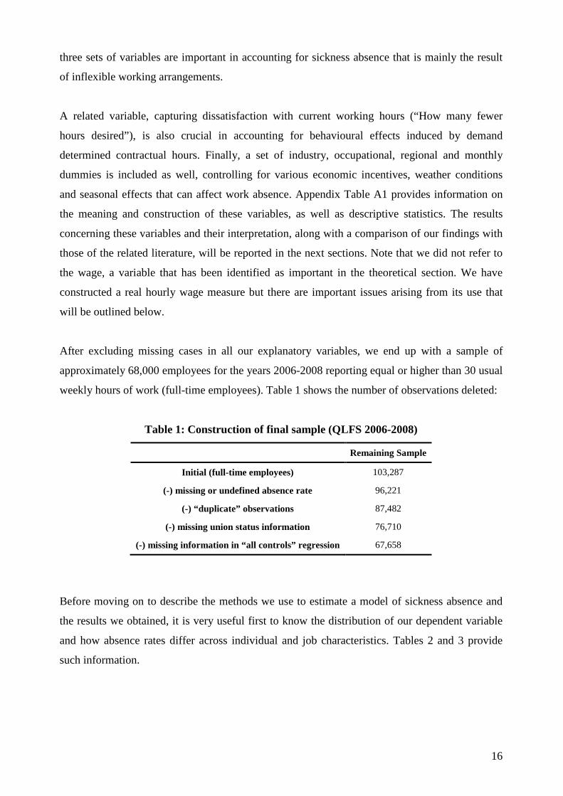
After excluding missing cases in all our explanatory variables, we end up with a sample of
approximately 68,000 employees for the years 2006-2008 reporting equal or higher than 30 usual
weekly hours of work (full-time employees). Table 1 shows the number of observations deleted:
Table 1: Construction of final sample (QLFS 2006-2008)
Remaining Sample
Initial (full-time employees) 103,287
(-) missing or undefined absence rate 96,221
(-) “duplicate” observations 87,482
(-) missing union status information 76,710
(-) missing information in “all controls” regression 67,658
Before moving on to describe the methods we use to estimate a model of sickness absence and
the results we obtained, it is very useful first to know the distribution of our dependent variable
and how absence rates differ across individual and job characteristics. Tables 2 and 3 provide
such information.

17
Table 2: Distribution of the Ordered Dependent Variable y
y = Frequency Percentage
0 64,967 96
1 1,061 1.6
2 314 0.5
3 1,316 2
Total 67,658 100
Note: Percentages do not sum to 100 due to rounding.
It is clear from Table 2 that the overwhelming majority of the individuals in our sample (96%)
did not miss any hour of work due to sickness in their reference week. Two percent of
employees, on the other hand, missed their entire week due to illness. Sensitivity to this “excess
zeros” problem will be explored in a secondary modelling approach in Section 7. Turning now to
Table 3, we can see that the average sickness absence rate for our sample equals 2.66% of total
working time.23 Moreover, we can see that union membership is associated with a higher
absence rate irrespective of the individual or job characteristic that we are looking at. The raw
union-nonunion differential in absence rates is 1.42 percentage points or 63.7% which provides
some first evidence that union membership is positively associated with higher weekly sickness
absence. Explicit modelling of the absence variable and multivariate statistical analysis is needed
in order to try to isolate the “pure” union membership effect on sickness absence.
Table 3: Absence Rates by Union Status (%)
All Union Non-union
All 2.66 3.65 2.23 Gender
Male 2.27 3.20 1.89 Female 3.25 4.21 2.77
Age 16-19 2.51 2.22 2.53 20-24 1.72 1.37 1.78
25-29 2 2.68 1.81 30-34 2.03 2.90 1.75 35-39 2.30 3.22 1.93 40-44 2.72 3.53 2.3 45-49 2.83 3.6 2.38 50-54 3.20 4.42 2.37 55-59 3.69 4.28 3.3 60-64 4.37 6.05 3.55
Ethnicity White 2.69 3.66 2.25 Mixed 2.01 2.86 1.72
23 For each group of individuals in each cell of Table 3, the absence rate given is the simple arithmetic mean of the absence rates in the reference week of the individuals belonging in that group. See Ercolani (2006) for various measures of presenting sickness absence rates by using the same methodology.

18
(Table 3 continued) Asian or Asian British 2.14 3.48 1.63 Black or Black British 3.45 3.71 3.29
Chinese 0.15 1.11 0 Other 2.36 4.01 1.82
Tenure (in months) 0-3 1.09 0.22 1.21 3-6 1.97 1.28 2.08
6-12 2.12 1.57 2.20 12-24 2.42 3.13 2.27 24-60 2.5 3.61 2.15
60-120 2.91 4.03 2.4 120-240 2.95 3.87 2.3
240+ 3.3 3.86 2.54 Establishment Size
1-24 2.2 3.29 1.98 25-49 2.86 3.82 2.5
50-499 2.72 3.64 2.24 500+ 3.08 3.77 2.5
Occupation
Managers and S.O. 1.69 2.64 1.48 Professionals 2.15 2.96 1.51
Ass. Profess. And Technical 2.74 3.48 2.23 Administrative and Secretarial 3.14 4.5 2.65
Skilled Trades 2.63 3.6 2.29 Personal Services 4.15 4.98 3.72
Sales and Customer Services 2.59 4.18 2.27 Plant and Machine Operatives 3.06 3.63 2.76
Elementary 3.62 4.97 3.05
Type of Contract
Permanent 2.68 3.68 2.23 Non-Permanent 2.04 1.86 2.09
Sector
Public 3.39 3.84 2.62 Private 2.39 3.4 2.17
Managerial/Supervisor Status
Manager/Foreman/Supervisor 2.27 3.07 1.9 No M/F/S 3 4.17 2.5
Marital Status
Married 2.6 3.49 2.16 Single 2.82 4.08 2.37
Health
Long-tem health problem 5.44 6.96 4.59 No long-term health problem 1.89 2.52 1.64
Year
2006 2.58 3.54 2.15 2007 2.76 3.68 2.35 2008 2.66 3.72 2.2
N 67,658 20,744 46,914 Note: Absence Rates refer to Average Sickness Absence Rates (mean of ratios), following the terminology in Ercolani (2006).
19
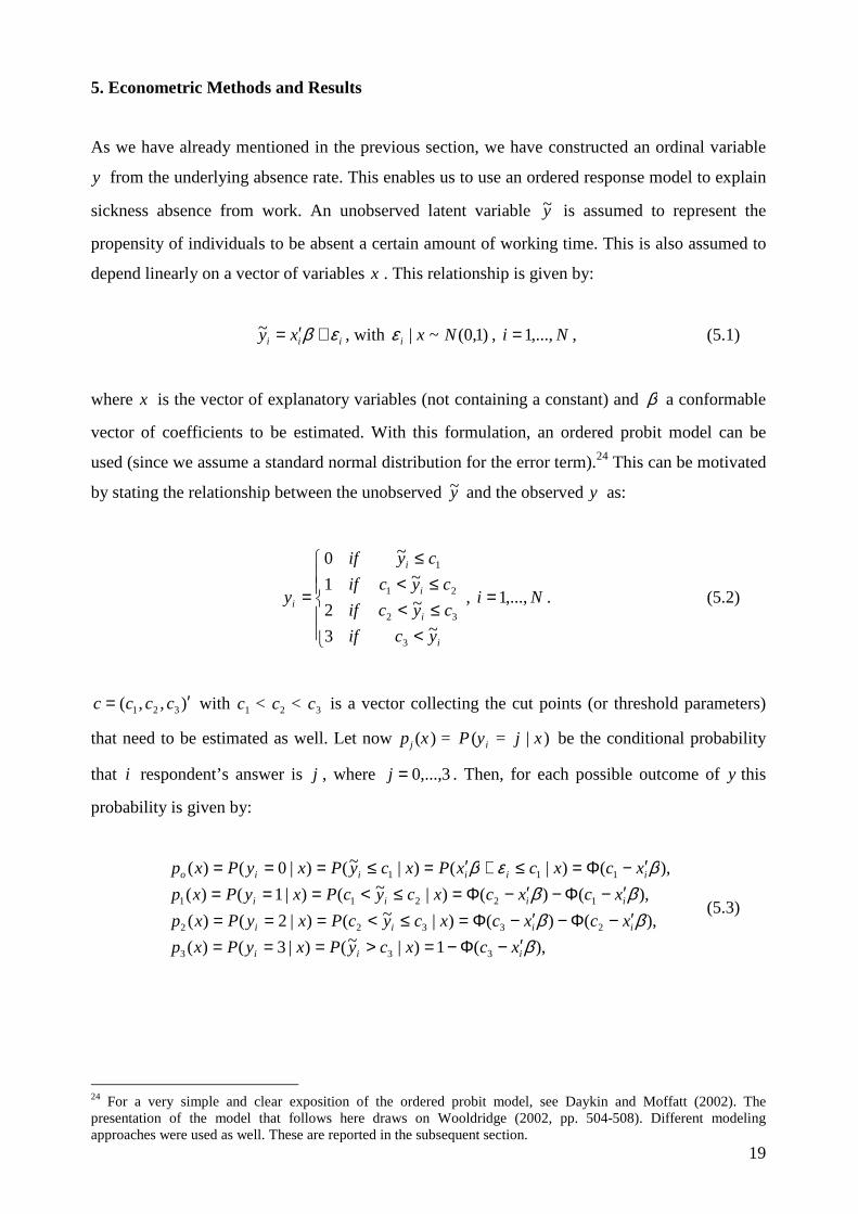
5. Econometric Methods and Results
As we have already mentioned in the previous section, we have constructed an ordinal variable
y from the underlying absence rate. This enables us to use an ordered response model to explain
sickness absence from work. An unobserved latent variable y~ is assumed to represent the
propensity of individuals to be absent a certain amount of working time. This is also assumed to
depend linearly on a vector of variables x . This relationship is given by:
iii xy εβ +′=~ , with )1,0(~| Nxiε , Ni ,...,1= , (5.1)
where x is the vector of explanatory variables (not containing a constant) and β a conformable
vector of coefficients to be estimated. With this formulation, an ordered probit model can be
used (since we assume a standard normal distribution for the error term).24 This can be motivated
by stating the relationship between the unobserved y~ and the observed y as:
<≤<≤<
≤
=
i
i
i
i
i
ycif
cycif
cycif
cyif
y
~3
~2
~1
~0
3
32
21
1
, Ni ,...,1= . (5.2)
),,( 321 ′= cccc with 1 2 3c c c< < is a vector collecting the cut points (or threshold parameters)
that need to be estimated as well. Let now ( ) ( | )j ip x P y j x= = be the conditional probability
that i respondent’s answer is j , where 3,...,0=j . Then, for each possible outcome of y this
probability is given by:
),(1)|~()|3()(
),()()|~()|2()(
),()()|~()|1()(
),()|()|~()|0()(
333
23322
12211
111
βββ
βββεβ
iii
iiii
iiii
iiiiio
xcxcyPxyPxp
xcxcxcycPxyPxp
xcxcxcycPxyPxp
xcxcxPxcyPxyPxp
′−Φ−=>===′−Φ−′−Φ=≤<===
′−Φ−′−Φ=≤<===′−Φ=≤+′=≤===
(5.3)
24 For a very simple and clear exposition of the ordered probit model, see Daykin and Moffatt (2002). The presentation of the model that follows here draws on Wooldridge (2002, pp. 504-508). Different modeling approaches were used as well. These are reported in the subsequent section.
20
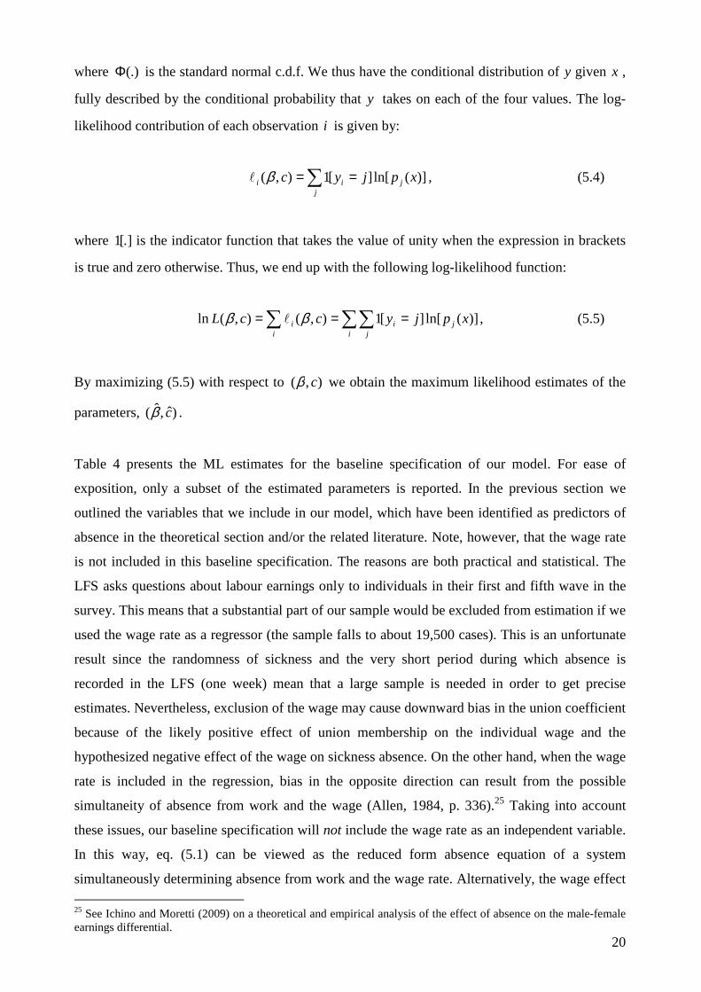
where (.)Φ is the standard normal c.d.f. We thus have the conditional distribution of y given x ,
fully described by the conditional probability that y takes on each of the four values. The log-
likelihood contribution of each observation i is given by:
∑ ==j
jii xpjyc )](ln[][1),(βl , (5.4)
where 1[.] is the indicator function that takes the value of unity when the expression in brackets
is true and zero otherwise. Thus, we end up with the following log-likelihood function:
∑∑∑ ===i j
jii
i xpjyccL )](ln[][1),(),(ln ββ l , (5.5)
By maximizing (5.5) with respect to ),( cβ we obtain the maximum likelihood estimates of the
parameters, )ˆ,ˆ( cβ .
Table 4 presents the ML estimates for the baseline specification of our model. For ease of
exposition, only a subset of the estimated parameters is reported. In the previous section we
outlined the variables that we include in our model, which have been identified as predictors of
absence in the theoretical section and/or the related literature. Note, however, that the wage rate
is not included in this baseline specification. The reasons are both practical and statistical. The
LFS asks questions about labour earnings only to individuals in their first and fifth wave in the
survey. This means that a substantial part of our sample would be excluded from estimation if we
used the wage rate as a regressor (the sample falls to about 19,500 cases). This is an unfortunate
result since the randomness of sickness and the very short period during which absence is
recorded in the LFS (one week) mean that a large sample is needed in order to get precise
estimates. Nevertheless, exclusion of the wage may cause downward bias in the union coefficient
because of the likely positive effect of union membership on the individual wage and the
hypothesized negative effect of the wage on sickness absence. On the other hand, when the wage
rate is included in the regression, bias in the opposite direction can result from the possible
simultaneity of absence from work and the wage (Allen, 1984, p. 336).25 Taking into account
these issues, our baseline specification will not include the wage rate as an independent variable.
In this way, eq. (5.1) can be viewed as the reduced form absence equation of a system
simultaneously determining absence from work and the wage rate. Alternatively, the wage effect
25 See Ichino and Moretti (2009) on a theoretical and empirical analysis of the effect of absence on the male-female earnings differential.
21
can be thought of being captured by variables such as the education and occupation dummies.
We briefly report on results based on specifications including the wage later in this section.26
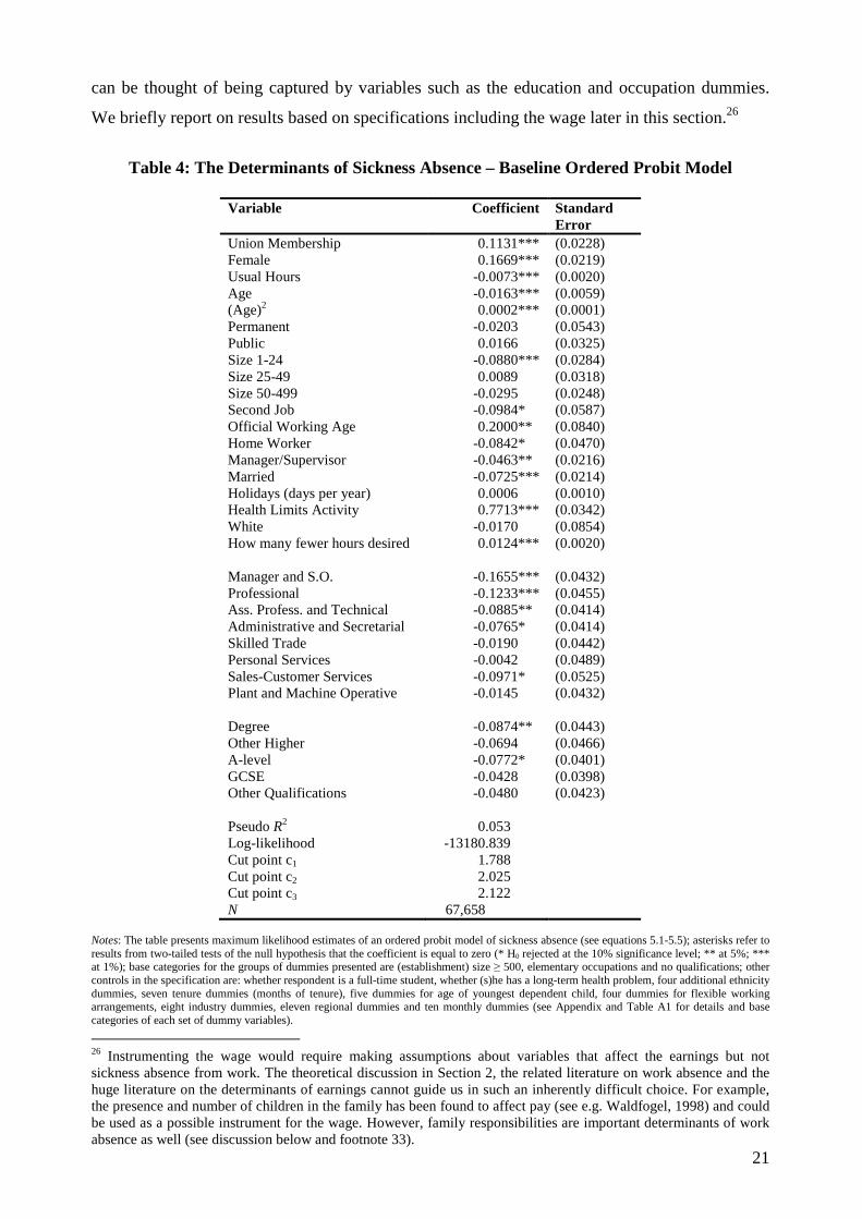
Table 4: The Determinants of Sickness Absence – Baseline Ordered Probit Model
Variable Coefficient
Standard Error
Union Membership 0.1131*** (0.0228) Female 0.1669*** (0.0219) Usual Hours -0.0073*** (0.0020) Age -0.0163*** (0.0059) (Age)2 0.0002*** (0.0001) Permanent -0.0203 (0.0543) Public 0.0166 (0.0325) Size 1-24 -0.0880*** (0.0284) Size 25-49 0.0089 (0.0318) Size 50-499 -0.0295 (0.0248) Second Job -0.0984* (0.0587) Official Working Age 0.2000** (0.0840) Home Worker -0.0842* (0.0470) Manager/Supervisor -0.0463** (0.0216) Married -0.0725*** (0.0214) Holidays (days per year) 0.0006 (0.0010) Health Limits Activity 0.7713*** (0.0342) White -0.0170 (0.0854) How many fewer hours desired 0.0124*** (0.0020) Manager and S.O. -0.1655*** (0.0432) Professional -0.1233*** (0.0455) Ass. Profess. and Technical -0.0885** (0.0414) Administrative and Secretarial -0.0765* (0.0414) Skilled Trade -0.0190 (0.0442) Personal Services -0.0042 (0.0489) Sales-Customer Services -0.0971* (0.0525) Plant and Machine Operative -0.0145 (0.0432) Degree -0.0874** (0.0443) Other Higher -0.0694 (0.0466) A-level -0.0772* (0.0401) GCSE -0.0428 (0.0398) Other Qualifications -0.0480 (0.0423) Pseudo R2 0.053 Log-likelihood -13180.839 Cut point c1 1.788 Cut point c2 2.025 Cut point c3 2.122 N 67,658
Notes: The table presents maximum likelihood estimates of an ordered probit model of sickness absence (see equations 5.1-5.5); asterisks refer to results from two-tailed tests of the null hypothesis that the coefficient is equal to zero (* H0 rejected at the 10% significance level; ** at 5%; *** at 1%); base categories for the groups of dummies presented are (establishment) size ≥ 500, elementary occupations and no qualifications; other controls in the specification are: whether respondent is a full-time student, whether (s)he has a long-term health problem, four additional ethnicity dummies, seven tenure dummies (months of tenure), five dummies for age of youngest dependent child, four dummies for flexible working arrangements, eight industry dummies, eleven regional dummies and ten monthly dummies (see Appendix and Table A1 for details and base categories of each set of dummy variables).
26 Instrumenting the wage would require making assumptions about variables that affect the earnings but not sickness absence from work. The theoretical discussion in Section 2, the related literature on work absence and the huge literature on the determinants of earnings cannot guide us in such an inherently difficult choice. For example, the presence and number of children in the family has been found to affect pay (see e.g. Waldfogel, 1998) and could be used as a possible instrument for the wage. However, family responsibilities are important determinants of work absence as well (see discussion below and footnote 33).
22
Due to the nonlinear nature of the ordered probit model, the estimated coefficients cannot be
directly interpreted. In ordered response models interest primarily lies not in the estimated
parameters per se, but on the estimated response probabilities and the change in them induced by
changes in the covariates of interest (the marginal effects). However, in Table 4 we can get a
picture of the direction and (statistical) difference from zero of the effect of right-hand side
variables on the underlying latent variable y~ (or, more formally, on )|~( xyE ), the propensity of
individuals to be absent a certain amount of working time.
Before focusing on the union membership impact on reported sickness absence, a brief
discussion concerning the other variables is required. A positive coefficient is estimated for the
female dummy. As it is widely acknowledged in the relevant literature women have higher
absence than men, ceteris paribus.27 In line with Barmby et al. (2004), we also find a negative
effect of usual working hours on absence. Recall that we include in the sample only full-time
employees (working over 30 hours a week) and for these high weekly hours this effect is
expected.28 Although this finding seems in contrast with the traditional labour-leisure choice
model (which does not distinguish between full-time and part-time workers), it can be interpreted
as an indication of a selection effect where employees with low propensity to be absent also tend
to work longer hours (Barmby et al., 2004, p.75). The same can be said about the finding
concerning the positive estimated coefficient on the “Working Age” dummy. Women who
choose or have to work above the official retirement age (59 years) should have strong
preferences against missing work, either because of economic necessity or because of a
distinctive “work ethic”. An additional explanation for this effect can be the better health status
of such employees. We can also draw upon the “economic necessity” argument to explain the
negative effect on sickness absence of having a second job (though this effect seems weaker and
is less precisely estimated29).
Health status matters a lot for sickness absence. Although this seems like a trivial observation, it
is important to mention it considering the low attention it receives in the economic and empirical
27 All studies cited in this chapter find this result. A more interesting issue seems to be the source of the male-female absence differential, something that is not of immediate interest to us. Specifically, one strand of the literature argues that the determinants of absence differ between men and women (Leigh, 1983; Vandenheuvel and Wooden, 1995; Bridges and Mumford, 2001). This approach can shed light on the sources of the gender absence gap. We briefly refer to this issue below. 28 In preliminary regressions, “squared usual hours” was also included in the model but its effect was not statistically different from zero. 29 The 90% confidence interval for the variable “Second Job” is [-0.195, -0.002]. Contrast it with the corresponding interval for the “Union” dummy: [0.076, 0.151].
23
models of absence behaviour.30 There is a variety of findings in these baseline specifications that
confirm that. The coefficient of the health variable reveals a very strong effect of long-term
health problems that limit daily work activity on work attendance.31 Also, the age of the
employee appears to have a U-shaped relationship with sickness absence, in line with the
findings of some studies (see, e.g., Allen, 1984, Table 1, p. 338). Younger workers are more
mobile and value leisure more than older ones. As they age their absence falls, but there is a
turning point where health issues start affecting their work attendance negatively.32
In the absence of the wage in the regressions, economic incentives can be captured with the
occupational and education dummies. Employees in white-collar occupations (managers-
officials, professionals and associate professionals) and with academic qualifications (degree
holders) are found to have lower sickness absence than blue-collar workers with low or no
qualifications. We can explain such findings with reference to the higher opportunity costs of
absence for such workers that are at the heart of the labour-leisure model (and its predicted
substitution effect of higher wages) or the labour-discipline approach. Supervisory status is also
found to be negatively related to absence, something that may also capture higher job
responsibilities.
What about family responsibilities? The premise of much of the related literature is that the
presence of a spouse and dependent children should affect absence behaviour and that there may
be a differential impact of such factors on male and female employees (VandenHeuvel and
Wooden, 1995; Bridges and Mumford, 2001), probably reflecting the traditional (male-centred)
societal expectations of the behaviour of women in the family context. Our baseline specification
can only answer the first empirical question, i.e. the effect of marital status and dependent
children on all employees irrespective of their gender. It is found here (as the coefficient of the
dummy “Married” reveals) that married workers tend to have a lower propensity to report sick,
possibly because of increased economic responsibilities towards the family. However, the
30 See Garcia-Serrano and Malo (2008) for an explicit empirical focus on health and disability and its impact on work absence of Spanish workers; see also Leigh (1991). 31 The strength of the estimated effect of any dummy can be assessed by comparing it to the size of the union membership effect that is presented below (see Table 5 and the relevant discussion there). Due to the non-linear nature of the model, however, the proportionate differences in the coefficients of two dummies do not mean equal proportionate differences in the effects of the variables they represent. 32 We cannot rule out the possibility that the strong effect of the health variables is partly the result of some form of self-justification bias where people that are absent more frequently tend to justify it by reference to their poor health. However, as it was made clear, the finding concerning the impact of the respondent’s age is also indicative of the overall importance of health for sickness absence.
24
presence of dependent children below the age of five increases absence, as is expected (results
not reported).33
In contrast with what the “adjustment-to-equilibrium” approach of the labour-leisure choice
model predicts, the possibility of taking some days off in terms of paid annual holidays or having
the opportunity of flexible working arrangements (Allen, 1981), do not appear to explain
sickness absence in our model. The coefficient of “Holidays” in Table 4 is close to zero and not
statistically different from that. A series of dummies capturing flexible working arrangements
(e.g. flexible working hours, annualized hours contract etc.) were all statistically insignificant
(estimates not reported).34 Concerning tenure, the only dummy that showed a statistically
significant effect was the one indicating a tenure period below 3 months ( 03ˆ
tenβ = -0.2091, s.e. =
0.0651 in the specification of Table 4, not reported there). This is a quite substantial effect and
shows that newly hired employees in their probationary period avoid reporting sick, possibly
because of fear of dismissal or limited/no sick-leave coverage.35
Workers in small workplaces are also less likely to be absent than workers in larger ones (see the
results for the “Size” dummies). This is in line with the argument by Winkelmann (1999), who
interprets this result as evidence in favour of a shirking hypothesis according to which employees
in larger establishments can be more easily absent without being detected. The demand-side
reasoning put forth by Barmby and Stephan (2000) also seems plausible: larger firms face lower
unit costs of absence since they are “able to diversify [absence] risk more easily” (Barmby and
Stephan, 2000, p. 571). Hence, on average, larger firms will have higher absence rates than
smaller ones. Note that this result is found with a union membership dummy present in the
model. This shows the empirical strength of this theoretical reasoning to some extent,
considering the strong positive correlation between firm size and union membership (see
Schnabel, 2003). The same thing cannot be said for another variable that is strongly correlated
33 In view of the arguments in some of the literature about a differential impact of family responsibilities on absence behaviour of men and women, a different specification containing full interactions between gender, marital status and presence of dependent children was estimated. Single women with no children were found to report more sickness absence than single men with no children ceteris paribus (a “pure” gender effect), while the most absence prone category was single female employees with dependent children of any age. In contrast, family responsibilities were not found to significantly affect the absence behaviour of male employees. There are some obvious policy implications of such findings. Further investigation of these issues, however, is beyond the scope of this chapter. 34 Working from home, an arrangement or job situation that can be considered as an important source of flexibility, is found to be negatively related with the propensity to report sick. This coefficient is relatively large but not so precisely estimated. 35 Temporary workers, on the other hand, do not report less sickness absence than permanent ones. If these workers are generally seeking a permanent contract within the firm they currently work, this result is counterintuitive. If, however, a large part of these employees works on temporary contracts because of the nature of their occupation (e.g. freelance or seasonal workers), the result makes more sense. See Engellandt and Riphahn (2005) for a careful empirical examination along these lines concerning temporary work and unpaid overtime.
25
with union membership, the public sector status of the employee. Once unionism is controlled
for, the public sector dummy has no substantial effect on sickness absence.36
Finally, it is worth noting that the variable capturing dissatisfaction with working hours (“How
many fewer hours desired”) is found to be positively related with sickness absence propensity.
This is an important control since it removes to some extent the effect of direct disagreement
with the current workload of the individuals in the sample, which may be thought as a strong
incentive of taking some (voluntary) absence. Also, it can deal to some extent with possible
endogeneity of union membership due to selection of dissatisfied employees into unions. The
estimated size of the union impact on sickness absence that will be presented in Table 5 below
refers to representative employees that do not state any dissatisfaction with their working hours.
This is a first indication that the strong positive effect of membership on sickness absence that
will be reported refers to genuine absence and the reduction in “presenteeism”. We later try to
elaborate on this point.
Let’s now turn to the main variable of interest. As already stated, union membership status is
found to exert a positive and strong effect on the amount of sickness absence. The “security”
union effect seems to be substantial and this can be shown by some additional calculations that
are needed to reveal the size of this impact. To this aim, Table 5 presents the absolute and
relative union membership effect on two outcome probabilities derived from the model (see eq.
(5.3)) and on the conditional expected value of sickness absence. The probabilities and expected
values are calculated for a representative male (Panel A) and female (Panel B) employee (see the
notes in Table 5 for the definition of each representative worker), given the estimates in our
baseline specification in Table 4. The probability of positive (or at least one hour of) absence is
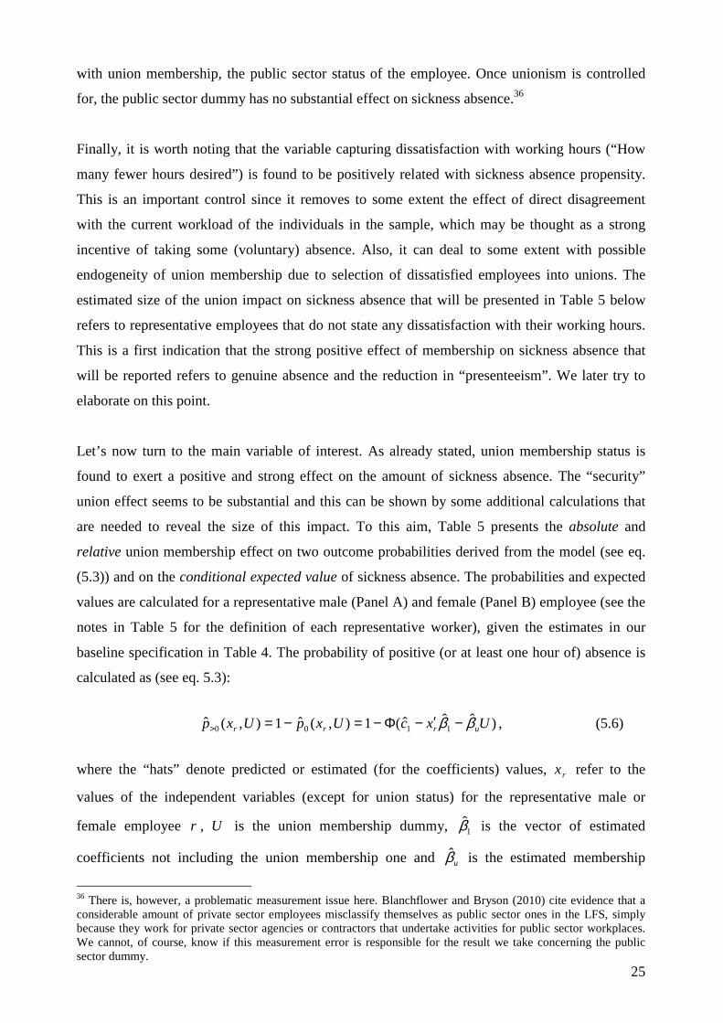
calculated as (see eq. 5.3):
)ˆˆˆ(1),(ˆ1),(ˆ 1100 UxcUxpUxp urrr ββ −′−Φ−=−=> , (5.6)
where the “hats” denote predicted or estimated (for the coefficients) values, rx refer to the
values of the independent variables (except for union status) for the representative male or
female employee r , U is the union membership dummy, 1̂β is the vector of estimated
coefficients not including the union membership one and uβ̂ is the estimated membership
36 There is, however, a problematic measurement issue here. Blanchflower and Bryson (2010) cite evidence that a considerable amount of private sector employees misclassify themselves as public sector ones in the LFS, simply because they work for private sector agencies or contractors that undertake activities for public sector workplaces. We cannot, of course, know if this measurement error is responsible for the result we take concerning the public sector dummy.
26
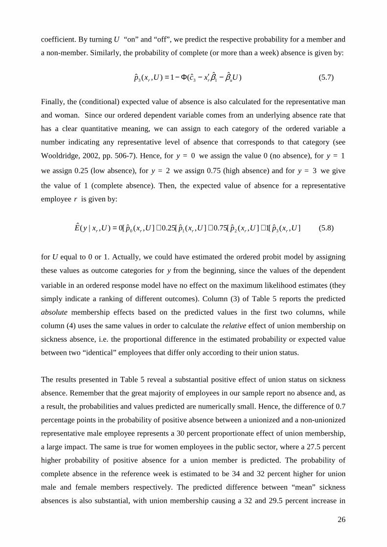
coefficient. By turning U “on” and “off”, we predict the respective probability for a member and
a non-member. Similarly, the probability of complete (or more than a week) absence is given by:
)ˆˆˆ(1),(ˆ 133 UxcUxp urr ββ −′−Φ−= (5.7)
Finally, the (conditional) expected value of absence is also calculated for the representative man
and woman. Since our ordered dependent variable comes from an underlying absence rate that
has a clear quantitative meaning, we can assign to each category of the ordered variable a
number indicating any representative level of absence that corresponds to that category (see
Wooldridge, 2002, pp. 506-7). Hence, for 0y = we assign the value 0 (no absence), for 1y =
we assign 0.25 (low absence), for 2y = we assign 0.75 (high absence) and for 3y = we give
the value of 1 (complete absence). Then, the expected value of absence for a representative
employee r is given by:
],(ˆ[1],(ˆ[75.0],(ˆ[25.0],(ˆ[0),|(ˆ3210 UxpUxpUxpUxpUxyE rrrrr +++= (5.8)
for U equal to 0 or 1. Actually, we could have estimated the ordered probit model by assigning
these values as outcome categories for y from the beginning, since the values of the dependent
variable in an ordered response model have no effect on the maximum likelihood estimates (they
simply indicate a ranking of different outcomes). Column (3) of Table 5 reports the predicted
absolute membership effects based on the predicted values in the first two columns, while
column (4) uses the same values in order to calculate the relative effect of union membership on
sickness absence, i.e. the proportional difference in the estimated probability or expected value
between two “identical” employees that differ only according to their union status.
The results presented in Table 5 reveal a substantial positive effect of union status on sickness
absence. Remember that the great majority of employees in our sample report no absence and, as
a result, the probabilities and values predicted are numerically small. Hence, the difference of 0.7
percentage points in the probability of positive absence between a unionized and a non-unionized
representative male employee represents a 30 percent proportionate effect of union membership,
a large impact. The same is true for women employees in the public sector, where a 27.5 percent
higher probability of positive absence for a union member is predicted. The probability of
complete absence in the reference week is estimated to be 34 and 32 percent higher for union
male and female members respectively. The predicted difference between “mean” sickness
absences is also substantial, with union membership causing a 32 and 29.5 percent increase in
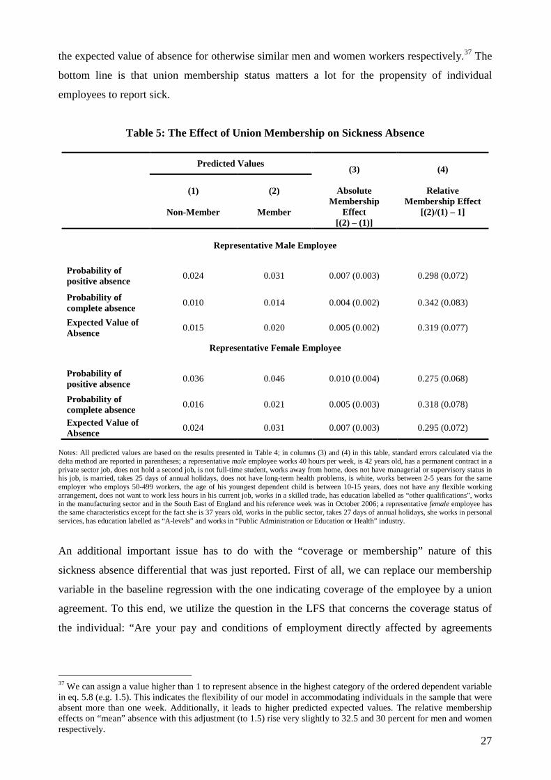
27
the expected value of absence for otherwise similar men and women workers respectively.37 The
bottom line is that union membership status matters a lot for the propensity of individual
employees to report sick.
Table 5: The Effect of Union Membership on Sickness Absence
Predicted Values (3)
Absolute
Membership Effect
[(2) – (1)]
(4)
Relative Membership Effect
[(2)/(1) – 1]
(1)
Non-Member
(2)
Member
Representative Male Employee
Probability of positive absence
0.024 0.031 0.007 (0.003) 0.298 (0.072)
Probability of complete absence
0.010 0.014 0.004 (0.002) 0.342 (0.083)
Expected Value of Absence
0.015 0.020 0.005 (0.002) 0.319 (0.077)
Representative Female Employee
Probability of positive absence
0.036 0.046 0.010 (0.004) 0.275 (0.068)
Probability of complete absence
0.016 0.021 0.005 (0.003) 0.318 (0.078)
Expected Value of Absence
0.024 0.031 0.007 (0.003) 0.295 (0.072)
Notes: All predicted values are based on the results presented in Table 4; in columns (3) and (4) in this table, standard errors calculated via the delta method are reported in parentheses; a representative male employee works 40 hours per week, is 42 years old, has a permanent contract in a private sector job, does not hold a second job, is not full-time student, works away from home, does not have managerial or supervisory status in his job, is married, takes 25 days of annual holidays, does not have long-term health problems, is white, works between 2-5 years for the same employer who employs 50-499 workers, the age of his youngest dependent child is between 10-15 years, does not have any flexible working arrangement, does not want to work less hours in his current job, works in a skilled trade, has education labelled as “other qualifications”, works in the manufacturing sector and in the South East of England and his reference week was in October 2006; a representative female employee has the same characteristics except for the fact she is 37 years old, works in the public sector, takes 27 days of annual holidays, she works in personal services, has education labelled as “A-levels” and works in “Public Administration or Education or Health” industry.
An additional important issue has to do with the “coverage or membership” nature of this
sickness absence differential that was just reported. First of all, we can replace our membership
variable in the baseline regression with the one indicating coverage of the employee by a union
agreement. To this end, we utilize the question in the LFS that concerns the coverage status of
the individual: “Are your pay and conditions of employment directly affected by agreements
37 We can assign a value higher than 1 to represent absence in the highest category of the ordered dependent variable in eq. 5.8 (e.g. 1.5). This indicates the flexibility of our model in accommodating individuals in the sample that were absent more than one week. Additionally, it leads to higher predicted expected values. The relative membership effects on “mean” absence with this adjustment (to 1.5) rise very slightly to 32.5 and 30 percent for men and women respectively.
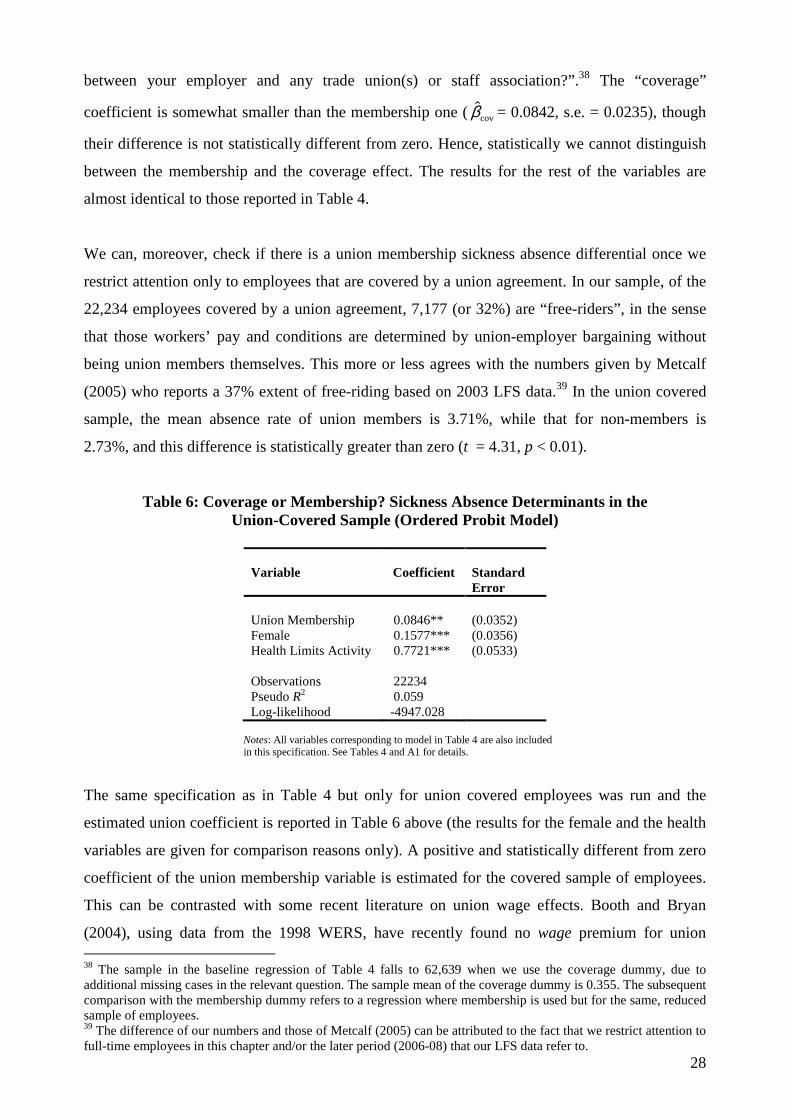
28
between your employer and any trade union(s) or staff association?”.38 The “coverage”
coefficient is somewhat smaller than the membership one ( covβ̂ = 0.0842, s.e. = 0.0235), though
their difference is not statistically different from zero. Hence, statistically we cannot distinguish
between the membership and the coverage effect. The results for the rest of the variables are
almost identical to those reported in Table 4.
We can, moreover, check if there is a union membership sickness absence differential once we
restrict attention only to employees that are covered by a union agreement. In our sample, of the
22,234 employees covered by a union agreement, 7,177 (or 32%) are “free-riders”, in the sense
that those workers’ pay and conditions are determined by union-employer bargaining without
being union members themselves. This more or less agrees with the numbers given by Metcalf
(2005) who reports a 37% extent of free-riding based on 2003 LFS data.39 In the union covered
sample, the mean absence rate of union members is 3.71%, while that for non-members is
2.73%, and this difference is statistically greater than zero (t = 4.31, p < 0.01).
Table 6: Coverage or Membership? Sickness Absence Determinants in the Union-Covered Sample (Ordered Probit Model)
Variable
Coefficient
Standard Error
Union Membership
0.0846**
(0.0352)
Female 0.1577*** (0.0356) Health Limits Activity 0.7721*** (0.0533) Observations 22234 Pseudo R2 0.059 Log-likelihood -4947.028
Notes: All variables corresponding to model in Table 4 are also included in this specification. See Tables 4 and A1 for details.
The same specification as in Table 4 but only for union covered employees was run and the
estimated union coefficient is reported in Table 6 above (the results for the female and the health
variables are given for comparison reasons only). A positive and statistically different from zero
coefficient of the union membership variable is estimated for the covered sample of employees.
This can be contrasted with some recent literature on union wage effects. Booth and Bryan
(2004), using data from the 1998 WERS, have recently found no wage premium for union 38 The sample in the baseline regression of Table 4 falls to 62,639 when we use the coverage dummy, due to additional missing cases in the relevant question. The sample mean of the coverage dummy is 0.355. The subsequent comparison with the membership dummy refers to a regression where membership is used but for the same, reduced sample of employees. 39 The difference of our numbers and those of Metcalf (2005) can be attributed to the fact that we restrict attention to full-time employees in this chapter and/or the later period (2006-08) that our LFS data refer to.
29
members in the covered sector, i.e. no wage incentive of covered non-members to join the
union.40 The findings here suggest that union membership may “pay” in a different way: covered
members seem to be able to consume more of the exclusive good of “protection against
disciplinary action” for “excessive” (from employers’ perspective) sickness absence than
covered non-members. Without additional qualitative information on actual practices of unions
in organized workplaces, we do not elaborate further on this finding.
Interpretation of the union membership effect on sickness absence
How can we interpret the strong positive impact of membership on sickness absence? Since we
control for long-term health problems of individuals in our model, the estimated union
coefficient cannot be attributed to selection into union membership of individuals with higher
absence propensity due to health reasons. In section 2 we outlined some possible channels that
relate union status with absence from work due to illness. Flexible working arrangements and
availability of paid holidays that can be affected by union bargaining are controlled for in our
regression and we reported above that these were not found to be significant determinants of
absence. Excluding them causes almost no change on the estimated union coefficient (uβ̂ =
0.114, s.e. = 0.023).
The impact through the union wage effect can be relevant here since we do not include the wage
in our baseline regression. We mentioned above that this exclusion can cause a downward bias in
the estimated union coefficient. The inclusion of the wage, on the other hand, can result in the
opposite bias (Allen, 1984). In order to have a complete picture, a specification including the
natural logarithm of the hourly wage rate was estimated.41 This specification refers to only a
limited subsample of our baseline one, because of the lack of earnings data. Table 7 presents the
results. Note that relative to our baseline model in Table 4, here the occupation and education
dummies are excluded since their effect on absence is hypothesized to mainly function through
the opportunity costs of absence (i.e. deferred wages) that higher occupation and education levels
entail.42 The two columns present two specifications where membership and coverage are used
interchangeably.
40 This result was also confirmed for the private sector by Blanchflower and Bryson (2010) who use the more recent wave of the WERS (2004). 41 See the Appendix for details on how we constructed an hourly wage rate using the LFS data. 42 We also keep only the “white” dummy in order to avoid perfect prediction that would naturally result from the significantly reduced sample size and the limited number of cases in some ethnicity categories.
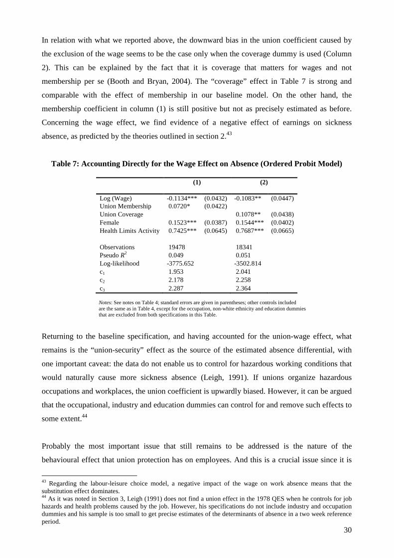
30
In relation with what we reported above, the downward bias in the union coefficient caused by
the exclusion of the wage seems to be the case only when the coverage dummy is used (Column
2). This can be explained by the fact that it is coverage that matters for wages and not
membership per se (Booth and Bryan, 2004). The “coverage” effect in Table 7 is strong and
comparable with the effect of membership in our baseline model. On the other hand, the
membership coefficient in column (1) is still positive but not as precisely estimated as before.
Concerning the wage effect, we find evidence of a negative effect of earnings on sickness
absence, as predicted by the theories outlined in section 2.43
Table 7: Accounting Directly for the Wage Effect on Absence (Ordered Probit Model)
(1)
(2)
Log (Wage) -0.1134*** (0.0432) -0.1083** (0.0447) Union Membership 0.0720* (0.0422) Union Coverage 0.1078** (0.0438) Female 0.1523*** (0.0387) 0.1544*** (0.0402) Health Limits Activity 0.7425*** (0.0645) 0.7687*** (0.0665) Observations 19478 18341 Pseudo R2 0.049 0.051 Log-likelihood -3775.652 -3502.814 c1 1.953 2.041 c2 2.178 2.258 c3 2.287 2.364
Notes: See notes on Table 4; standard errors are given in parentheses; other controls included are the same as in Table 4, except for the occupation, non-white ethnicity and education dummies that are excluded from both specifications in this Table.
Returning to the baseline specification, and having accounted for the union-wage effect, what
remains is the “union-security” effect as the source of the estimated absence differential, with
one important caveat: the data do not enable us to control for hazardous working conditions that
would naturally cause more sickness absence (Leigh, 1991). If unions organize hazardous
occupations and workplaces, the union coefficient is upwardly biased. However, it can be argued
that the occupational, industry and education dummies can control for and remove such effects to
some extent.44
Probably the most important issue that still remains to be addressed is the nature of the
behavioural effect that union protection has on employees. And this is a crucial issue since it is
43 Regarding the labour-leisure choice model, a negative impact of the wage on work absence means that the substitution effect dominates. 44 As it was noted in Section 3, Leigh (1991) does not find a union effect in the 1978 QES when he controls for job hazards and health problems caused by the job. However, his specifications do not include industry and occupation dummies and his sample is too small to get precise estimates of the determinants of absence in a two week reference period.
31
disregarded in almost all theoretical and empirical analyses of work (and, specifically, sickness)
absence determinants, though its normative and policy implications are obvious. In Section 2 and
3 we commented on how absence from work is viewed in the relevant literature and the problems
of interpretation that this view has. To fix ideas, first recall what our absence measure refers to: it
counts contracted working hours lost due to illness, indirectly derived from the relevant survey
questions to UK employees in the LFS. Why this absence should be exclusively voluntary (i.e.
“shirking”) is less than obvious. There is no reason why an employee will respond that he was
absent from work due to sickness in the reference week when the real reason was something else
(irrespective of the reason given to the employer) and he is given the opportunity in the LFS to
report it. But even if this is the case for some self-reported sickness absence recorded in the LFS,
it cannot be ruled out that a significant part of what we observe is genuine absence.
Having said that, the interpretation of the membership absence differential can lead to normative
conclusions largely different from the accounts in CBI (2008), that view absence only as a cost
to the employer, and in Ichino and Riphahn (2005) that theoretically stress the adverse effects of
job protection on shirking behaviour. These accounts of sickness absence as “absenteeism” are
based on abstract theoretical reasoning or formal models and not on a proper interpretation of
what is actually observed in the data and what the estimated parameters actually tell us.45 The
reduction in “presenteeism” (i.e. increase in genuine sickness absence) that results from union
protection and found here can be an efficiency enhancing mechanism from the point of view of
both employees and firms, to a large extent correcting for inefficiently strict disciplinary rules for
absence and non-generous replacement rates. And this is at least an equally plausible
interpretation given the definition of our dependent variable (and the way the underlying data
were obtained) and the empirical analysis that we undertook.
Is there a way actually to distinguish between genuine and non-genuine sickness absence given
the LFS questions? And can we offer evidence that our preferred interpretation of the
membership absence differential is valid? Though such an attempt cannot be completely
successful due to the nature of the data, it is possible to construct a different absence rate from
the LFS data. Following the procedure in Section 4, we now code 1is = when the respondent
reports that he worked fewer hours than usual in the reference week because of “other reasons”.
45 Ichino and Riphahn (2005) use data from a large Italian bank and their “absence due to illness” variable is computed from the bank’s records. Hence, their interpretation of absence as shirking is probably more relevant in their case since the data come from the employer. However, in their theoretical model, genuinely sick workers will always report sick. First, this is in contrast with some available evidence of extensive “presenteeism” among employees (see Heymann et al., 2009, and Hemp, 2004, for US accounts; see also the discussion in Section 2). Second, such a theoretical assumption means that the increase in absence observed after employment protection is guaranteed (their theoretical hypothesis) can only be explained by increased shirking, not decreased “presenteeism”.
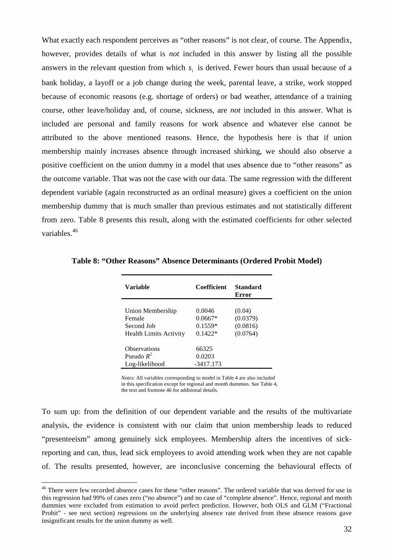
32
What exactly each respondent perceives as “other reasons” is not clear, of course. The Appendix,
however, provides details of what is not included in this answer by listing all the possible
answers in the relevant question from which is is derived. Fewer hours than usual because of a
bank holiday, a layoff or a job change during the week, parental leave, a strike, work stopped
because of economic reasons (e.g. shortage of orders) or bad weather, attendance of a training
course, other leave/holiday and, of course, sickness, are not included in this answer. What is
included are personal and family reasons for work absence and whatever else cannot be
attributed to the above mentioned reasons. Hence, the hypothesis here is that if union
membership mainly increases absence through increased shirking, we should also observe a
positive coefficient on the union dummy in a model that uses absence due to “other reasons” as
the outcome variable. That was not the case with our data. The same regression with the different
dependent variable (again reconstructed as an ordinal measure) gives a coefficient on the union
membership dummy that is much smaller than previous estimates and not statistically different
from zero. Table 8 presents this result, along with the estimated coefficients for other selected
variables.46
Table 8: “Other Reasons” Absence Determinants (Ordered Probit Model)
Variable
Coefficient
Standard Error
Union Membership
0.0046
(0.04)
Female 0.0667* (0.0379) Second Job Health Limits Activity
0.1559* 0.1422*
(0.0816) (0.0764)
Observations 66325 Pseudo R2 0.0203 Log-likelihood -3417.173
Notes: All variables corresponding to model in Table 4 are also included in this specification except for regional and month dummies. See Table 4, the text and footnote 46 for additional details.
To sum up: from the definition of our dependent variable and the results of the multivariate
analysis, the evidence is consistent with our claim that union membership leads to reduced
“presenteeism” among genuinely sick employees. Membership alters the incentives of sick-
reporting and can, thus, lead sick employees to avoid attending work when they are not capable
of. The results presented, however, are inconclusive concerning the behavioural effects of
46 There were few recorded absence cases for these “other reasons”. The ordered variable that was derived for use in this regression had 99% of cases zero (“no absence”) and no case of “complete absence”. Hence, regional and month dummies were excluded from estimation to avoid perfect prediction. However, both OLS and GLM (“Fractional Probit” - see next section) regressions on the underlying absence rate derived from these absence reasons gave insignificant results for the union dummy as well.

33
membership on sick-reporting, since it cannot be ruled out that union protection can also lead to
increased shirking. But if sickness absence is viewed more broadly as it was the aim here,
popular calculations of absence costs (CBI, 2008) can be misleading.47
6. Sensitivity Checks
A possible objection to the results presented in the previous section is that they depend heavily
on the modelling procedure we follow. To address this, we modelled sickness absence in various
different ways in order to check whether our conclusions concerning the union membership
impact are still valid. In sum, the main conclusions of the previous section remain almost
identical, irrespective of the model and the estimator used.
First, the simple ordered probit model may be inadequate in capturing the process of absence
behaviour. Harris and Zhao (2007) postulate that when the dependent variable is characterized by
an excessive number of zeros (as is our case here) two different processes may be at work.
Adapting their tobacco consumption case to the dependent variable in this paper, the absence
decision can be conceptualized as occurring in two consecutive stages: in the first stage, the
individual decides whether or not to be absent; in the second one, and conditional on
“participating”, the amount of absence is determined. However, this second-stage amount of
absence can be zero. Hence, in order for a positive amount of sickness absence to be observed,
two “hurdles” should be overcome: the employee should first decide participation in absence
“consumption” and, then, that he is a “non-zero consumption” participant. When the absence
behaviour is conceptualized in this way and the outcome variable is an ordinal measure, a zero-
inflated ordered probit model is an appropriate one. The difference with the ordered probit
model presented in the previous section is that a participation decision is additionally modelled
here as a binary choice and, then, a probit model can be used. The outcome probabilities in eq.
(5.3) and, hence, the likelihood function, are then adjusted accordingly in order to reflect the fact
that they are affected by the first-stage decision of participation (or not). Harris and Zhao (2007,
pp.1075-6) present the analytical details.
A parsimonious specification of our baseline model was chosen for the zero-inflated
specification. First, it was assumed that the same variables affect both the participation decision
and the second-stage “consumption” decision. Second, a subset of the variables used in the 47 A possible objection to the results presented in this section concerns the endogeneity of union membership. Selection of workers into union status according to their absence propensity may bias the results. However, there is no obvious way in the LFS to deal with this issue. Its panel element is very short, while suitable instruments for union membership status are not available.
34
model presented in Table 4 was kept in the zero-inflated one. This was necessary in order to be
feasible to estimate the parameters (i.e. to achieve convergence at a maximum in our log-
likelihood function) via standard numerical procedures.48 For comparison, we also estimated the
respective ordered probit model with this subset of covariates. The results for the remaining
variables are almost the same as the ones in Table 4 (for example, uβ̂ = 0.1163, s.e. = 0.022).
In the zero-inflated ordered probit model, union membership was estimated to positively affect
both the participation and the amount of “consumption” (conditional on participation). In order
to compare the union effect in the zero-inflated model with that in the simple ordered probit one,
the membership effect on the probability of at least one hour of absence (or positive absence)
was calculated, in line with the approach in Table 5. For the representative male employee, the
relative membership effect (that corresponds to Column 4, Line 1 in Table 5) is predicted to be
0.273, i.e. a male union member has a 27.3 percent higher probability of at least one hour of
absence in the reference week compared with a similar male non-union employee. The respective
effect in the simple ordered probit model was calculated approximately equal to 30 percent. This
similarity in the predictions of the two models was also confirmed through the other measures of
the membership effect analogous with those in Table 5 (see below, Table 9).
There seems, however, no important reason to prefer the zero-inflated model over the simple
ordered probit one. Statistically, the two information-based criteria for model selection (AIC and
BIC) provided contradictory results.49 Theoretically, nothing in our discussion in Section 2
pointed to a modelling based on a “double-hurdle” approach. Harris and Zhao’s (2007)
motivation for the zero-inflated model refers to tobacco consumption decisions. Alcohol
consumption or crime behaviour can also be cases where a double-hurdle model can be justified.
In the case of sickness absence, however, a much more detailed and structured theory is required
in order to justify such a modelling procedure. To be more precise, one should theorize about the
determinants of absence behaviour at each stage, which variables affect (and how) the
“participation” and the subsequent “consumption” decision, what is the role of union
48 The independent variables that we used in this modelling approach are (see Table 4 for comparison): union, female, usual hours, age, age squared, permanent, public, establishment size dummies, second job, working age, home worker, manager/supervisor, married, holidays, health limits activity, how many fewer hours desired, education, industry and regional dummies. Occupation dummies were replaced by a dummy indicating blue-collar status (occupation categories 5-9 in Table A1), tenure was limited to a dummy indicating tenure under 3 months or not, ethnicity was limited to a white-nonwhite dummy only and for age of youngest dependent child only two dummies were used, the first indicating an age under 10 years and the second indicating age equal or higher than 10 years. 49 For the zero-inflated ordered probit (“ZIOP”) we obtained the values AICziop = 26246.95 and BICziop = 27238.93. For the ordered probit (“OP”), AICop = 26534.51 and BICop = 27040.62. The preferred model is the one with the smaller AIC or BIC. Therefore, the two criteria give opposite results. See Harris and Zhao (2007, p. 1079) for the specific formulas.
35
membership or union bargaining in this more complicated picture and so on. Practically, our
conclusions concerning the membership effect are the same.
Directly modelling the absence rate without relying on an ordinal measure is another way to
check the sensitivity of our results. A simple linear model can be specified and estimated by
OLS. The conditional mean is given by βxxRE ′=)|( , where R is the sickness absence rate
defined in Section 4. The problem is that OLS is probably invalid in our case since R is a
fractional variable, i.e. constrained between zero and one. Hence, we also use the quasi
maximum likelihood estimator proposed by Papke and Wooldridge (1996) for the case of a
fractional dependent variable. In this approach, a function (.)G , satisfying 0 ( ) 1G z< < for all
ℜ∈z is used for modelling the conditional mean and then a Bernoulli log-likelihood function is
maximized to obtain the parameter estimates. We here assume )()( zzG Φ= , where (.)Φ is the
standard normal c.d.f. (i.e. we specify a “fractional probit” model), in order to keep the
distributional assumption consistent across the models in this chapter. The conditional mean in
this model is, thus, given by )()|( βxxRE ′Φ= .50
Qualitatively, the results from both OLS and the fractional probit are almost identical for all the
variables with those reported in Table 4 (ordered probit). Quantitatively, the OLS union
coefficient is 0.0084 with a standard error of 0.0016, while the ML estimate of the fractional
probit is 0.126 (s.e. = 0.024). Thus, OLS results indicate an approximately 0.85 percentage
points’ difference between the expected absence of a union and a similar non-union employee.
This predicted absolute membership effect is identical for an “average” or a representative
employee in the case of OLS due to the linearity of the model, but not in the case of the
fractional probit. The estimated coefficient in the latter model indicates that a union member has
0.7 percentage points’ higher average absence than a comparable (average) non-member
employee.51
In order to get a final picture of the similarity of the membership effect across the different
models, we also predicted the expected value of sickness absence and the union membership
effect for the representative male employee of Table 5. The following Table 9 presents these
calculations for the three non-linear models that we referred to in this section (ordered probit,
50 See Papke and Wooldridge (1996) for further details. Using the logistic function for modelling the conditional mean and, hence, specifying a “fractional logit” model, produces, as expected, very similar results with the ones reported below. The same also holds for the complementary log-log function that relaxes the symmetry of the standard normal and the logistic distribution functions. 51 This number refers to the marginal effect of union membership on expected sickness absence calculated at all the variables’ sample means.
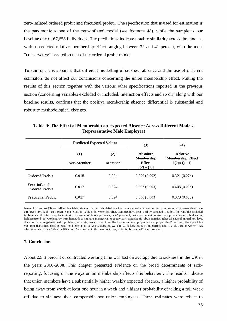
36
zero-inflated ordered probit and fractional probit). The specification that is used for estimation is
the parsimonious one of the zero-inflated model (see footnote 48), while the sample is our
baseline one of 67,658 individuals. The predictions indicate notable similarity across the models,
with a predicted relative membership effect ranging between 32 and 41 percent, with the most
“conservative” prediction that of the ordered probit model.
To sum up, it is apparent that different modelling of sickness absence and the use of different
estimators do not affect our conclusions concerning the union membership effect. Putting the
results of this section together with the various other specifications reported in the previous
section (concerning variables excluded or included, interaction effects and so on) along with our
baseline results, confirms that the positive membership absence differential is substantial and
robust to methodological changes.
Table 9: The Effect of Membership on Expected Absence Across Different Models (Representative Male Employee)
Predicted Expected Values (3)
Absolute
Membership Effect
[(2) – (1)]
(4)
Relative Membership Effect
[(2)/(1) – 1]
(1)
Non-Member
(2)
Member
Ordered Probit 0.018 0.024 0.006 (0.002) 0.321 (0.074)
Zero-Inflated Ordered Probit
0.017 0.024 0.007 (0.003) 0.403 (0.096)
Fractional Probit 0.017 0.024 0.006 (0.003) 0.379 (0.093)
Notes: In columns (3) and (4) in this table, standard errors calculated via the delta method are reported in parentheses; a representative male employee here is almost the same as the one in Table 5; however, his characteristics have been slightly adjusted to reflect the variables included in these specifications (see footnote 48): he works 40 hours per week, is 42 years old, has a permanent contract in a private sector job, does not hold a second job, works away from home, does not have managerial or supervisory status in his job, is married, takes 25 days of annual holidays, does not have long-term health problems, is white, works over 3 months for the same employer who employs 50-499 workers, the age of his youngest dependent child is equal or higher than 10 years, does not want to work less hours in his current job, is a blue-collar worker, has education labelled as “other qualifications” and works in the manufacturing sector in the South-East of England.
7. Conclusion
About 2.5-3 percent of contracted working time was lost on average due to sickness in the UK in
the years 2006-2008. This chapter presented evidence on the broad determinants of sick-
reporting, focusing on the ways union membership affects this behaviour. The results indicate
that union members have a substantially higher weekly expected absence, a higher probability of
being away from work at least one hour in a week and a higher probability of taking a full week
off due to sickness than comparable non-union employees. These estimates were robust to

37
different modelling and estimation techniques. To a large extent, the result presented here can be
attributed to the protection that unions offer to employees in unionized workplaces. There is also
some evidence that this union protection reduces “presenteeism” among genuinely sick
employees. This finding has broad implications for the way economists view absence from work
and can provide support for theoretical modelling that is consistent with these results, through an
explicit focus on the difference between voluntary and involuntary absence.
38
REFERENCES
Addison J. and Belfield C., 2001, “Updating the Determinants of Firm Performance: Estimation Using the 1998 UK Workplace Employee Relations Survey”, British Journal of Industrial Relations, vol.39, no.3, pp.341-366. -------- and --------, 2002, “Unions and Establishment Performance: Evidence from the British Workplace Industrial/Employee Relations Survey”, IZA Discussion Paper No.455. Allen S. G., 1981, “An Empirical Model of Work Attendance”, The Review of Economics and Statistics, vol.63, no.1, pp.77-87. --------, 1981b, “Compensation, Safety, and Absenteeism: Evidence from the Paper Industry”, Industrial and Labor Relations Review, vol.34, no.2, pp.207-218. --------, 1983, “How Much Does Absenteeism Cost?”, Journal of Human Resources, vol.18, no.3, pp.379-393. --------, 1984, “Trade Unions, Absenteeism and Exit-Voice”, Industrial and Labour Relations Review, vol.37, no.3, pp.331-345. Balchin J. and Wooden M., 1995, “Absence Penalties and Work Attendance”, Australian Economic Review, vol.28, no.4, pp.43-58. Barmby T. and Larguem M., 2007, “Coughs and Sneezes Spread Diseases: An Empirical Study of Absenteeism and Infectious Illness”, mimeo. -------- and Stephan G., 2000, “Worker Absenteeism: Why Firm Size May Matter”, The Manchester School, vol.68, no.5, pp.568-577. --------, Ercolani M. and Treble J., 2004, “Sickness Absence in the UK 1984-2002”, Swedish Economic Policy Review, vol.11, pp.65-88. Blanchflower D. and Bryson A., 2003, “Changes Over Time in Union Relative Wage Effects in the UK and USA Revisited”, in J. Addison and C. Schnabel (eds), International Handbook of Trade Unions, Cheltenham: Edward Elgar. -------- and --------, 2010, “The Wage Impact of Trade Unions in the UK Public and Private Sectors”, Economica, vol.77, no.305, pp.92-109. -------- and Freeman R., 1992, “Unionism in the United States and other Advanced OECD Countries”, Industrial Relations, vol.31, no.1, pp.56-79. Booth A. and Bryan M., 2004, “The Union Membership Wage-Premium Puzzle: Is There a Free Rider Problem?”, Industrial and Labor Relations Review, vol.57, no.3, pp.402-421. Bridges S. and Mumford K., 2001, “Absenteeism in the UK: A Comparison Across Genders”, The Manchester School, vol.69, no.3, pp.276-284. Brown S. and Sessions J., 1996, “The Economics of Absence: Theory and Evidence”, Journal of Economic Surveys, vol.10, no.1, pp.23-53.

39
Budd J. and Mumford K., 2004, “Trade Unions and Family-Friendly Policies in Britain”, Industrial and Labor Relations Review, vol.57, no.2, pp.204-222. CBI, 2008, At Work and Working Well? CBI/AXA Absence and Labour Turnover Survey, London: CBI. Chadwick-Jones J. K., Brown C. A. and Nicholson A., 1973, “A-type and B-type Absence: Empirical Trends for Women Employees”, Occupational Psychology, vol.47, pp.75-80. Chatterji M. and Tilley C., 2002, “Sickness, Absenteeism, Presenteeism, and Sick Pay”, Oxford Economic Papers, vol.54, pp.669-687. Daykin A. R. and Moffatt P. G., 2002, “Analyzing Ordered Responses: A Review of the Ordered Probit Model”, Understanding Statistics, vol.1, no.3, pp.157-166. Drago R. and Wooden M., 1992, “The Determinants of Labor Absence: Economic Factors and Workgroup Norms Across Countries”, Industrial and Labor Relations Review, vol.45, no.4, pp.764-778. Engellandt A. and Riphahn R. T., 2005, “Temporary Contracts and Employee Effort”, Labour Economics, vol.12, pp.281-299. Ercolani M., 2006, “UK Employees’ Sickness Absence: 1984-2005”, mimeo, Department of Economics, University of Birmingham. Farber H., 2001, “Trade Unions: Empirical Analyses”, in N. J. Smelser and P. B. Baltes (eds), International Encyclopedia of the Social and Behavioral Sciences, Oxford: Elsevier. Fernie S. and Metcalf D., 1995, “Participation, Contingent Pay, Representation and Workplace Performance: Evidence from Great Britain”, British Journal of Industrial Relations, vol.33, no.3, pp.379-415. Freeman R., 1976, “Individual Mobility and Union Voice in the Labour Market”, American Economic Review, vol.66, no.2, pp.361-368. Frick B. and Malo M. Á., 2008, “Labor Market Institutions and Individual Absenteeism in the European Union: The Relative Importance of Sickness Benefit Systems and Employment Protection Legislation”, Industrial Relations, vol.47, no.4, pp.505-529. Garcia-Serrano C. and Malo M. Á., 2008, “The Influence of Disability on Absenteeism: An Empirical Analysis Using Spanish Data”, ISER Working Paper No. 2008-29, September. -------- and --------, 2009, “The Impact of Union Direct Voice on Voluntary and Involuntary Absence”, The Journal of Socio-Economics, vol.38, pp.372-383. Gimeno D., Benavides F. G., Benach J. and Amick III B. C., 2004, “Distribution of Sickness Absence in the European Union Countries”, Occupational and Environmental Medicine, vol.61, pp.867-869. Green F., 1997, “Union Recognition and Paid Holiday Entitlement”, British Journal of Industrial Relations, vol.35, no.2, pp.243-255.
40
Harris M. N. and Zhao X., 2007, “A Zero-Inflated Ordered Probit Model, With an Application to Modelling Tobacco Consumption”, Journal of Econometrics, vol.141, pp.1073-1099. Hemp P., 2004, “Presenteeism: At Work – But Out of It”, Harvard Business Review, vol.82, no.10, pp.49-58, October. Heymann J., Rho H. J., Schmitt J. and Earle A., 2009, “Contagion Nation: A Comparison of Paid Sick Day Policies in 22 Countries”, Center for Economic and Policy Research Briefing Paper, May. Ichino A. and Moretti E., 2009, “Biological Gender Differences, Absenteeism, and the Earnings Gap”, American Economic Journal: Applied Economics, vol.1, no.1, pp.183-218. -------- and Riphahn R. T., 2005, “The Effect of Employment Protection on Worker Effort: Absenteeism During and After Probation”, Journal of the European Economic Association, vol.3, no.1, pp.120-143. Kenyon P. and Dawkins P., 1989, “A Time Series Analysis of Labour Absence in Australia”, The Review of Economics and Statistics, vol.71, no.2, pp.232-239. Leaker D., 2008, “Sickness Absence from Work in the UK”, Economic and Labour Market Review, vol.2, no.11, pp.18-22. Leigh J. P., 1981, “The Effects of Union Membership on Absence from Work due to Illness”, Journal of Labor Research, vol.2, no.2, pp.329-336. --------, 1984, “Sex Differences in Absenteeism”, Industrial Relations, vol.22, no.3, pp.349-361. --------, 1984, “Unionization and Absenteeism”, Applied Economics, vol.16, pp.147-157. --------, 1986, “Correlates of Absence from Work Due to Illness”, Human Relations, vol.39, no.1, pp.81-100. --------, 1991, “Employee and Job Attributes as Predictors of Absenteeism in a National Sample of Workers: The Importance of Health and Dangerous Working Conditions”, Social Science and Medicine, vol.33, no.2, pp.127-137. Luchak A. A. and I. R. Gellatly, 1996, “Exit-Voice and Employee Absenteeism: A Critique of the Industrial Relations Literature”, Employee Responsibilities and Rights Journal, vol.9, no.2, pp.91-102. Metcalf D., 2005, “Trade Unions: Resurgence or Perdition? An Economic Analysis”, in S. Fernie and D. Metcalf (eds), Trade Unions: Resurgence or Decline? The Future of trade unions in Britain, London: Routledge. Minister Law Solicitors, 2009, “Workers Fear Over Sick Days”, press release, 16 January, available at http://newsroom.minsterlaw.co.uk/page.php?page_id=15&story=2007 (accessed on 29 April 2009). Osterkamp R. and Röhn O., 2007, “Being on Sick Leave: Possible Explanations for Differences of Sick-leave Days Across Countries”, CESifo Economic Studies, vol.53, no.1, pp.97-114.
41
Papke L. and Wooldridge J., 1996, “Econometric Methods for Fractional Response Variables with an Application to 401(k) Plan Participation Rates”, Journal of Applied Econometrics, vol.11, pp.619-632. Paringer L., 1983, “Women and Absenteeism: Health or Economics?”, American Economic Review, vol.73, no.2, pp.123-127. Schnabel C., 2003, “Determinants of trade union membership”, in J. Addison and C. Schnabel (eds), International Handbook of Trade Unions, Cheltenham: Edward Elgar. Steers R. M. and Rhodes S. R., 1978, “Major Influences on Employee Attendance: A Process Model”, Journal of Applied Psychology, vol.63, no.4, pp.391-407. Stewart M. B. and Swaffield J. K., 1997, “Constraints on the Desired Hours of Work of British Men”, Economic Journal, vol.107, pp.520-535. Unite, 2008, Absence in the Workplace, pamphlet available at www.amicustheunion.org. VandenHeuvel A. and Wooden M., 1995, “Do Explanations of Absenteeism Differ Between Men and Women?”, Human Relations, vol.48, no.11, pp.1309-1329. Waldfogel J., 1998, “Understanding the ‘Family Gap’ in Pay for Women with Children”, Journal of Economic Perspectives, vol.12, no.1, pp.137-156. Winkelmann R., 1999, “Wages, Firm Size and Absenteeism”, Applied Economics Letters, vol. 6, pp.337-341. Wooldridge J., 2002, Econometric Analysis of Cross Section and Panel Data, Cambridge, MA: MIT Press.
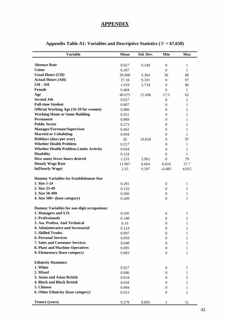
42
APPENDIX
Appendix Table A1: Variables and Descriptive Statistics (N = 67,658)
Variable Mean Std. Dev. Min Max
Absence Rate 0.027 0.149 0 1 Union 0.307 0 1 Usual Hours (UH) 39.008 5.364 30 80 Actual Hours (AH) 37.18 9.101 0 97 UH - AH 1.019 5.734 0 80 Female 0.404 0 1 Age 40.675 11.696 17.5 62 Second Job 0.027 0 1 Full-time Student 0.007 0 1 Official Working Age (16-59 for women) 0.988 0 1 Working Home or Same Building 0.051 0 1 Permanent 0.969 0 1 Public Sector 0.273 0 1 Manager/Foreman/Supervisor 0.462 0 1 Married or Cohabiting 0.694 0 1 Holidays (days per year) 26 10.634 0 97 Whether Health Problem 0.217 0 1 Whether Health Problem Limits Activity 0.034 0 1 Disability 0.124 0 1 How many fewer hours desired 1.233 3.961 0 79 Hourly Wage Rate 11.967 6.664 0.616 57.7 ln(Hourly Wage) 2.35 0.507 -0.485 4.055 Dummy Variables for Establishment Size 1. Size 1-24 0.291 0 1 2. Size 25-49 0.132 0 1 3. Size 50-499 0.366 0 1 4. Size 500+ (base category) 0.209 0 1 Dummy Variables for one-digit occupations: 1. Managers and S.O. 0.195 0 1 2. Professionals 0.148 0 1 3. Ass. Profess. And Technical 0.16 0 1 4. Administrative and Secretarial 0.124 0 1 5. Skilled Trades 0.097 0 1 6. Personal Services 0.059 0 1 7. Sales and Customer Services 0.048 0 1 8. Plant and Machine Operatives 0.085 0 1 9. Elementary (base category) 0.083 0 1 Ethnicity Dummies: 1. White 0.927 0 1 2. Mixed 0.006 0 1 3. Asian and Asian British 0.034 0 1 4. Black and Black British 0.018 0 1 5. Chinese 0.004 0 1 6. Other Ethnicity (base category) 0.012 0 1 Tenure (years) 9.279 8.895 1 51
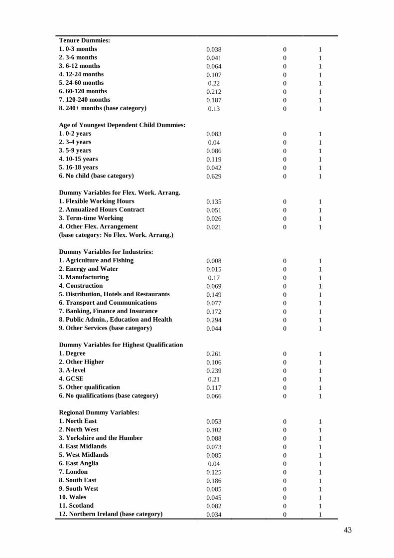
43
Tenure Dummies: 1. 0-3 months 0.038 0 1 2. 3-6 months 0.041 0 1 3. 6-12 months 0.064 0 1 4. 12-24 months 0.107 0 1 5. 24-60 months 0.22 0 1 6. 60-120 months 0.212 0 1 7. 120-240 months 0.187 0 1 8. 240+ months (base category) 0.13 0 1 Age of Youngest Dependent Child Dummies: 1. 0-2 years 0.083 0 1 2. 3-4 years 0.04 0 1 3. 5-9 years 0.086 0 1 4. 10-15 years 0.119 0 1 5. 16-18 years 0.042 0 1 6. No child (base category) 0.629 0 1 Dummy Variables for Flex. Work. Arrang. 1. Flexible Working Hours 0.135 0 1 2. Annualized Hours Contract 0.051 0 1 3. Term-time Working 0.026 0 1 4. Other Flex. Arrangement 0.021 0 1 (base category: No Flex. Work. Arrang.) Dummy Variables for Industries: 1. Agriculture and Fishing 0.008 0 1 2. Energy and Water 0.015 0 1 3. Manufacturing 0.17 0 1 4. Construction 0.069 0 1 5. Distribution, Hotels and Restaurants 0.149 0 1 6. Transport and Communications 0.077 0 1 7. Banking, Finance and Insurance 0.172 0 1 8. Public Admin., Education and Health 0.294 0 1 9. Other Services (base category) 0.044 0 1 Dummy Variables for Highest Qualification 1. Degree 0.261 0 1 2. Other Higher 0.106 0 1 3. A-level 0.239 0 1 4. GCSE 0.21 0 1 5. Other qualification 0.117 0 1 6. No qualifications (base category) 0.066 0 1 Regional Dummy Variables: 1. North East 0.053 0 1 2. North West 0.102 0 1 3. Yorkshire and the Humber 0.088 0 1 4. East Midlands 0.073 0 1 5. West Midlands 0.085 0 1 6. East Anglia 0.04 0 1 7. London 0.125 0 1 8. South East 0.186 0 1 9. South West 0.085 0 1 10. Wales 0.045 0 1 11. Scotland 0.082 0 1 12. Northern Ireland (base category) 0.034 0 1

44
Dummies for Years and Months: 2008 0.356 0 1 2007 0.321 0 1 2006 0.323 0 1 Oct-06 (base category) 0.128 0 1 Nov-06 0.105 0 1 Dec-06 0.089 0 1 Sep-07 0.025 0 1 Oct-07 0.098 0 1 Nov-07 0.103 0 1 Dec-07 0.095 0 1 Sep-08 0.001 0 1 Oct-08 0.114 0 1 Nov-08 0.143 0 1 Dec-08 0.098 0 1
Note: All numbers are rounded to the third decimal place; base categories refer to the dummies of each group excluded from the regression in Table 4.
Notes on Variables: Most variables and their construction is self-explanatory, however, for some of them it is
required to give a brief description of what they mean and how we constructed them from the LFS data.
Absence Rate: The definition of this measure and more details are provided in Section 4. For usual hours, the
derived variable “BUSHR” in the LFS is used. This variable comes from various questions concerning usual
working hours and excludes overtime. Only employees with usual weekly working hours between 30 and 80 are
kept in the sample. For actual hours, the derived “BACTHR” is used, that also excludes overtime. The question
“YLESS6” is used for the construction of the dummy si. This question states: “What was the main reason that you
did fewer hours than usual/were away from work in the week ending Sunday the [date]”. The possible answers are
the following:
1) Number of hours worked/overtime varies 2) Bank holiday 3) Maternity or paternity leave 4) Parental leave 5) Other leave/holiday 6) Sick or injured 7) Attending a training course away from own workplace 8) Started new job/ changed jobs 9) Ended job and did not start new one that week 10) Laid off/short time/work interrupted by bad weather 11) Laid off/short time/work interrupted by labour dispute at own workplace 12) Laid off/short time/work interrupted by economic and other causes 13) Other personal/family reasons 14) Other reasons
Answer 6, “sick or injured”, leads to si = 1 for the sickness absence measure. Answers 13 (“other personal/family
reasons”) and 14 (“other reasons”) are used to code si = 1 for the alternative “other reasons” absence measure that
was briefly mentioned and used in Section 6.
Age: The original variable in the LFS questionnaire was banded (see Table 3 for the categories). In the regression
analysis and in Table A1, we have made this variable continuous by assigning the mid-point for each age category.
45
Health problems: These refer to long-term health problems reported by the employee. The relevant question is: “Do
you have any health problems or disabilities that you expect will last more than a year?”. If the answer is “yes”, the
first variable relating to health in the above table is coded as 1. If no, it is coded as 0. The employees that answered
“yes” are then asked if that health problem affects the amount of paid work that they might do. The answer to this
second question is used to create the second health variable reported in the above table (1 = yes [it affects it]; 0 = no
[it does not]). “Disability” is created by a derived variable (“discurr”) coded by the LFS administrators. We code
“disability” as 1 if “discurr” refers to individuals that are “both DDA disabled and work-limiting disabled” or “DDA
disabled only” or “Work-limiting disabled only”. Our three variables cannot be used together in a regression since
the last one is actually derived by the first two.
How many fewer hours desired: The employee is asked whether he would like to work fewer hours in his/her current
job even if that meant less pay. If (s)he answers “yes”, (s)he is then asked “How many fewer hours would you like to
work in that / your current job?”. The amount is recorded and constitutes the variable here. If (s)he answered “no”
in the first question, the variable is given a zero value. Responses that exceed 80 hours are dropped since we have
restricted our sample to employees reporting equal or less than 80 usual weekly hours worked.
Hourly Wage Rate: The gross weekly pay reported in the LFS is converted into hourly pay by using the formula
gross weekly payhourly pay
1.5UH POT=
+, where UH is the number of usual weekly hours worked and POT is the usual
amount of paid overtime worked per week; then, the hourly wages for the workers in 2007 and 2008 are deflated to
2006 prices by using the Consumer Price Indices for the October-December quarters reported by the Office for
National Statistics; we have trimmed the distribution of gross weekly pay by excluding the lowest and highest 1%.
Because of the way the income questions are asked in the LFS (only in their first and last/fifth wave interviewees
provide information about their earnings), the sample when the wage is included in regressions drops to 19,478.
Tenure: We report in Table A1 two measures for tenure; the first is one continuous variable measuring tenure in
years; the second is a set of dummy variables that measures tenure with current employer in months; we use the
second set of variables in the regressions.
Age of youngest dependent child dummies: As it is noted in the text, in some specifications (e.g. Section 6 and
Table 9) only 3 categories are used, combining the ones presented in the Table A1 above; these categories are: age
of youngest dependent child is under 10 (sample mean 0.21), equal or over 10 (0.162) and no child (0.629, as
above).