understanding radiation thermometry

Understanding Radiation Thermometry 1Tim Risch

Understanding Radiation

Thermometry – Part IITimothy K. Risch

NASA Armstrong Flight Research Center

July 8, 2015


Part I

End off Part 1

Lesson Plan

Nomenclature

Introduction

History of Radiation Thermometry

Fundamental Physics

Practical Radiation Thermometers

Practical Measurement

Techniques

Calibration

Final Thoughts

For Further Reading

Part II


Preliminaries

An Excel® worksheet containing solutions to all examples are available from Tim Risch at [email protected]

Excel®, Visual Basic for Applications®, and Microsoft® are registered trademarks of Microsoft Corporation.

mailto:[email protected]


Nomenclature - I

𝑐 speed of light, 2.99792458 × 108 m/s

𝐶1 Planck’s first constant, 2 ℎ𝑐2 = 1.191043 × 108 W-m4/m2-sr

𝐶2 Planck’s second constant, ℎ𝑐/𝑘 = 14,387.75 m-K

𝐶3 Constant in Wien’s displacement law

𝐶4 Constant in equation for maximum blackbody intensity

𝐷𝑖 detector spectral response function for detector i

ℎ Planck’s constant, 6.626068 × 10-34 J-s

𝑘 Boltzmann constant, 1.3806503 × 10-23 J/K

𝑖𝑏,𝜆(, 𝑇) spectral emissive radiance of a perfect blackbody at wavelength and temperature 𝑇, W/m2-sr-m

𝑖𝜆(, 𝑇) spectral radiant intensity of a non-blackbody at wavelength and temperature 𝑇, W/m2-sr-m


Nomenclature - II

𝑖𝑏(𝑇) total radiant intensity of a blackbody at temperature 𝑇,

W/m2-sr-m

𝑖(𝑇) total radiant intensity non-blackbody at temperature 𝑇,

W/m2-sr-m

𝑇 actual surface temperature, K

𝑇𝑟 ratio temperature, K

𝑇 measured surface temperature at wavelength assuming a

perfect emitter, K


Nomenclature - III

𝑇 total emissivity of a non-blackbody at temperature 𝑇

𝑖 wavelength-averaged emissivity for detector 𝑖

𝑟 wavelength averaged emissivity ratio for detector 1 and 2, 2/ 1

𝜆 monochromatic emissivity of a non-blackbody at wavelength

and temperature 𝑇

𝑇 inferred total emissivity of a non-blackbody at temperature 𝑇

𝑟 emissivity ratio at two wavelengths 1 and 2, 12

Δ𝑖 bandwidth of narrow-band detector i, m

Λ equivalent wavelength, 𝜆1𝜆2 (𝜆2− 𝜆1), m

𝜆𝑖 wavelength of detector i, m


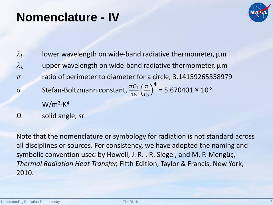
Nomenclature - IV

𝜆𝑙 lower wavelength on wide-band radiative thermometer, m

𝜆𝑢 upper wavelength on wide-band radiative thermometer, m

𝜋 ratio of perimeter to diameter for a circle, 3.14159265358979

σ Stefan-Boltzmann constant, 𝜋𝐶1

15

𝜋

𝐶2

4= 5.670401 × 10-8

W/m2-K4

Ω solid angle, sr

Note that the nomenclature or symbology for radiation is not standard across all disciplines or sources. For consistency, we have adopted the naming and symbolic convention used by Howell, J. R. , R. Siegel, and M. P. Mengüç, Thermal Radiation Heat Transfer, Fifth Edition, Taylor & Francis, New York, 2010.


Practical Measurement Techniques

“To point out of the advantages that would arise from ascertaining the heat of a body at a very high temperature would be unnecessary, the importance of the subject is allowed.”- J. M’Sweeny, M.D. - 1829


Radiation Temperature Measurement - I

For a blackbody, there are three primary ways to determine the temperature by measuring:

› The total emitted radiation

› The distribution across wavelengths or the total radiation across a wavelength band

› The emitted radiation at one wavelength

Measuring any of these should uniquely determine the temperature


Radiation Temperature Measurement - II

As discussed before, real surfaces with emissivities less than one do not behave like a blackbody.

Instead, they emit radiation at rates less than a blackbody

This introduces a new problem, for any given measurement of a non-ideal surface, we now have two unknowns:

› Temperature

› Emissivity

Without assuming either one or the other, the state of the surface cannot be uniquely determined.


Three Possible Solutions:

1. For a single measurement, assume the emissivity and calculate the temperature (spectral method)

2. Make two measurements at different wavelengths and assume a relationship between the emissivities at each wavelength and calculate a single temperature (ratio method)

3. Make multiple measurements at different wavelengths and assume some functional form of the emissivity and find the best fit to the temperature and emissivity (multi-spectral method)

For now, all of the examples assume narrow-band detectors, but later we show how to accommodate wide-band detectors


Some Temperature Definitions

“True” Surface Temperature - The actual temperature of the surface; what we would measure with a thermometer not affected by the surface emissivity. This is the temperature we would measure if, for example, we used a contact thermometer such as a thermocouple.

“Equivalent Blackbody” Surface Temperature - The temperature we would infer from a radiation thermometer if we assumed that the surface was a perfect emitter. Again, because all real surfaces emit less than a blackbody, the equivalent blackbody surface temperature will always be lower than the true surface temperature.


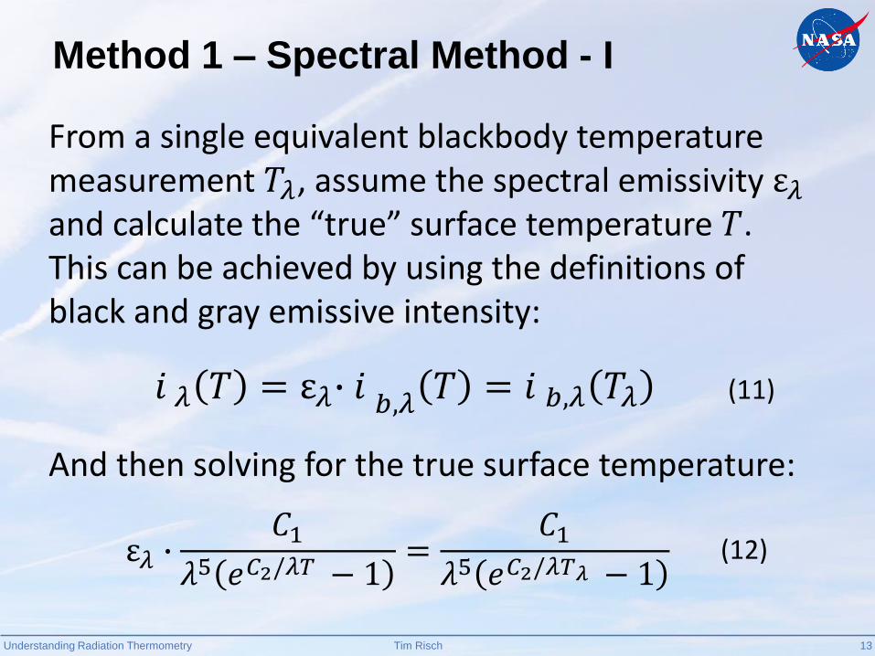
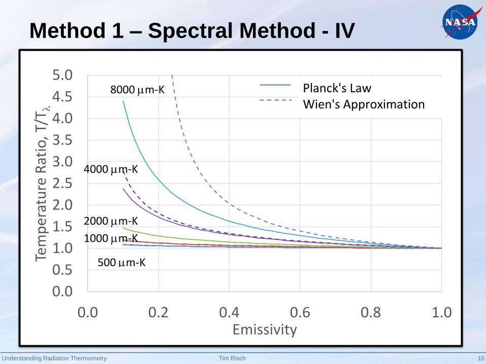
Method 1 – Spectral Method - I

From a single equivalent blackbody temperature measurement 𝑇𝜆, assume the spectral emissivity ε𝜆and calculate the “true” surface temperature 𝑇. This can be achieved by using the definitions of black and gray emissive intensity:

And then solving for the true surface temperature:

𝑖 𝜆 𝑇 = ε𝜆∙ 𝑖 𝑏,𝜆 𝑇 = 𝑖 𝑏,𝜆 𝑇𝜆 (11)

ε𝜆 ∙𝐶1

𝜆5 𝑒𝐶2/𝜆𝑇 − 1=

𝐶1𝜆5 𝑒𝐶2/𝜆𝑇𝜆 − 1

(12)


Solving for true surface temperature this is:

Equation 13 can be simplified under the special case when 𝐶2/𝜆𝑇𝜆 ≫ 1 (Wien’s approximation) then:

1

𝑇=

𝜆

𝐶2ln ε𝜆 ∙ 𝑒

𝐶 2 𝜆𝑇𝜆 − 1 + 1 (13)

1

𝑇=

1

𝑇𝜆+

𝜆

𝐶2ln ε𝜆 (14)

Method 1 – Spectral Method - II


0.0

0.5

1.0

1.5

2.0

2.5

3.0

3.5

4.0

4.5

5.0

0.0 0.2 0.4 0.6 0.8 1.0

Tem

pe

ratu

re R

atio

, T/T

Emissivity

500 m-K

1000 m-K

2000 m-K

4000 m-K

8000 m-K Planck's LawWien's Approximation

Method 1 – Spectral Method - IV


Example 4 - I

E4: What is the true surface temperature when a surface at an equivalent blackbody temperature of 3,820 K is measured with a 0.5-𝜇m wavelength detector and an emissivity of 0.8 is assumed?


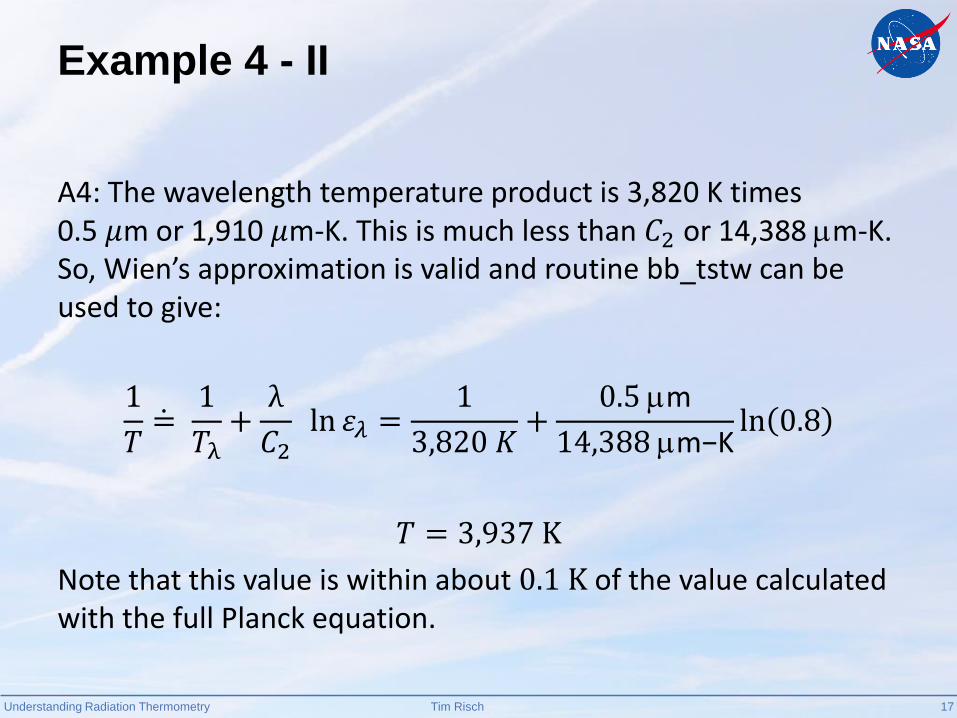
Example 4 - II

A4: The wavelength temperature product is 3,820 K times 0.5 𝜇m or 1,910 𝜇m-K. This is much less than 𝐶2 or 14,388 m-K. So, Wien’s approximation is valid and routine bb_tstw can be used to give:

1

𝑇 =1

𝑇λ+

λ

𝐶2ln 𝜀𝜆 =

1

3,820 𝐾+

0.5 m

14,388 m−Kln 0.8

𝑇 = 3,937 K

Note that this value is within about 0.1 K of the value calculated with the full Planck equation.


Example 5 - I

E5: Repeat Example 4, except with an 8-𝜇m detector. What is the true surface temperature?


Example 5 - II

A5: The wavelength temperature product is 3,820 K times 8 𝜇m or 30,560 𝜇m-K. This is greater than 𝐶2 or 14,388 m-K. So, the full Planck equation (Equation 1) must be used using routine bb_tst:

𝑇 =𝐶2/𝜆

ln ε𝜆 ∙ 𝑒𝐶 2 𝜆𝑇𝜆 − 1 + 1

𝑇 = 14,388 m−K 8 𝜇m

ln 0.8 ∙ 𝑒 14,388 m−K 8 𝜇m 3820 𝐾 − 1 + 1= 4,579 K

If indeed we had used Wien’s approximation, the calculated true surface temperature would have been over 7,200 K and off by over 2,600 K.


We can see by looking at Equation 13, that the correction to the measured surface temperature is dependent on the wavelength and when Wien’s approximation applies in Equation 14, the correction is proportional to the wavelength. This suggests that using a short wavelength detector will minimize the effect of emissivity on our temperature measurement.

Method 1 – Spectral Method - V


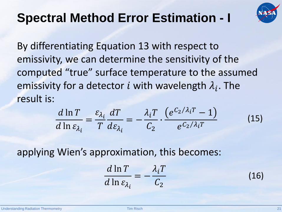
Spectral Method Error Estimation - I

By differentiating Equation 13 with respect to emissivity, we can determine the sensitivity of the computed “true” surface temperature to the assumed emissivity for a detector 𝑖 with wavelength 𝜆𝑖. The result is:

applying Wien’s approximation, this becomes:

𝑑 ln 𝑇

𝑑 ln 𝜀𝜆𝑖=𝜀𝜆𝑖𝑇

𝑑𝑇

𝑑𝜀𝜆𝑖= −

𝜆𝑖𝑇

𝐶2∙𝑒 𝐶2 𝜆𝑖𝑇 − 1

𝑒 𝐶2 𝜆𝑖𝑇(15)

𝑑 ln 𝑇

𝑑 ln 𝜀𝜆𝑖= −

𝜆𝑖𝑇

𝐶2(16)


Using the sensitivity and an estimate of the uncertainty in the emissivity produces an estimate of the uncertainty in the surface temperature:

∆𝑇

𝑇=

𝑑 ln 𝑇

𝑑 ln 𝜀𝜆𝑖∙∆𝜀𝜆𝑖𝜀𝜆𝑖

(17)

Spectral Method Error Estimation - II


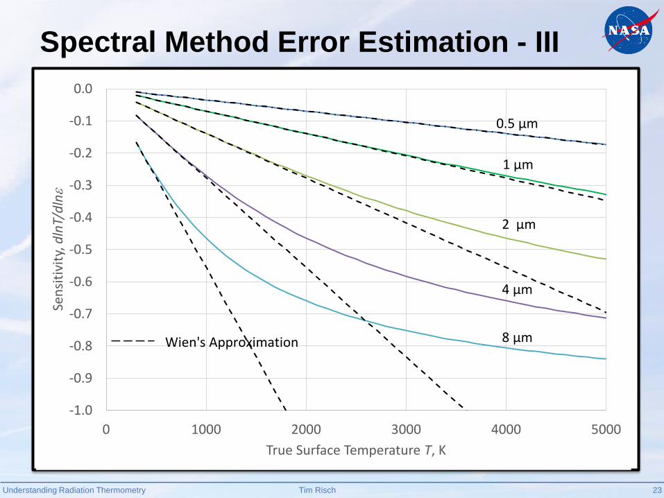
Spectral Method Error Estimation - III

-1.0

-0.9

-0.8

-0.7

-0.6

-0.5

-0.4

-0.3

-0.2

-0.1

0.0

0 1000 2000 3000 4000 5000

Sen

siti

vity

, dln

T/d

ln

True Surface Temperature T, K

0.5 µm

1 µm

2 µm

4 µm

8 µmWien's Approximation


Example 6 - I

E6: If the spectral emissivity of graphite at 0.53 𝜇m is estimated to be 0.8 with an estimated uncertainty of 20%, what is the estimated uncertainty in the temperature if a detector at this wavelength indicates an equivalent blackbody temperature of 2,950 K?


Example 6 - II

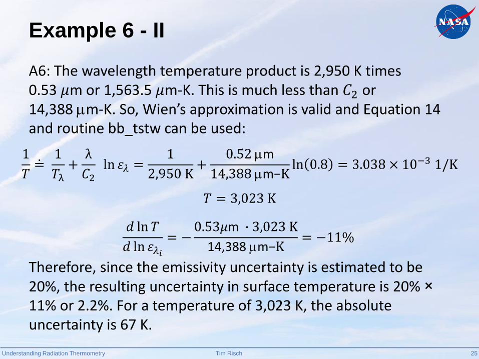
A6: The wavelength temperature product is 2,950 K times 0.53 𝜇m or 1,563.5 𝜇m-K. This is much less than 𝐶2 or 14,388 m-K. So, Wien’s approximation is valid and Equation 14 and routine bb_tstw can be used:

Therefore, since the emissivity uncertainty is estimated to be 20%, the resulting uncertainty in surface temperature is 20% ×11% or 2.2%. For a temperature of 3,023 K, the absolute uncertainty is 67 K.

𝑑 ln 𝑇

𝑑 ln 𝜀𝜆𝑖= −

0.53𝜇m ∙ 3,023 K

14,388 m−K= −11%

1

𝑇 =1

𝑇λ+

λ

𝐶2ln 𝜀𝜆 =

1

2,950 K+

0.52 m

14,388 m−Kln 0.8 = 3.038 × 10−3 1/K

𝑇 = 3,023 K


Example 7 - I

E7: Repeat example 6 except for a detector with a wavelength of 5.8 𝜇m where the emissivity is estimated to be 0.8 with an estimated uncertainty of 20% at a temperature of 2,950 K.


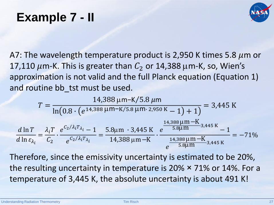
Example 7 - II

A7: The wavelength temperature product is 2,950 K times 5.8 𝜇m or 17,110 𝜇m-K. This is greater than 𝐶2 or 14,388 m-K, so, Wien’s approximation is not valid and the full Planck equation (Equation 1) and routine bb_tst must be used.

𝑇 = 14,388 m−K 5.8 𝜇m

ln 0.8 ∙ 𝑒 14,388 m−K 5.8 m∙ 2,950 K − 1 + 1= 3,445 K

𝑑 ln 𝑇

𝑑 ln 𝜀𝜆𝑖=𝜆𝑖𝑇

𝐶2∙𝑒

𝐶2 𝜆𝑖𝑇𝜆𝑖 − 1

𝑒 𝐶2 𝜆𝑖𝑇𝜆𝑖

=5.8m ∙ 3,445 K

14,388 m−K∙𝑒14,388m−K

5.8m ∙3,445 K− 1

𝑒14,388m−K

5.8m ∙3,445 K

= −71%

Therefore, since the emissivity uncertainty is estimated to be 20%, the resulting uncertainty in temperature is 20% × 71% or 14%. For a temperature of 3,445 K, the absolute uncertainty is about 491 K!


Rule 1

When the emissivity is unknown and must be estimated, the most accurate surface temperature measurement is made when a detector with a wavelength as short as possible is used.


Determination of Emissivities at Other Wavelengths

Once the true surface temperature has been determined from a detector at one wavelength, the emissivity at other detector wavelengths can be determined from:

Of course, using a measurement at the same wavelength will return our initial guess for 𝜀𝜆.

𝜀𝜆 =𝑒𝐶2/𝜆𝑇 − 1

𝑒𝐶2/𝜆𝑇𝜆 − 1(18)


Emissivity Uncertainty Estimation - I

The uncertainty in the emissivity at a second wavelength 𝜀𝜆𝑖based on the estimated uncertainty in a

given wavelength 𝜀𝜆1 is, by differentiation:

If Wien’s approximation is valid at both wavelengths then:

𝑑 ln 𝜀𝜆𝑖𝑑 ln 𝜀𝜆1

=𝜀𝜆1𝜀𝜆𝑖

∙𝑑𝜀𝜆𝑖𝑑𝜀𝜆1

=𝜆1𝜆𝑖∙𝑒 −𝐶2 𝜆1𝑇 − 1

𝑒 −𝐶2 𝜆𝑖𝑇 − 1(19)

𝑑 ln 𝜀𝜆𝑖𝑑 ln 𝜀𝜆1

=𝜆1𝜆𝑖

(20)


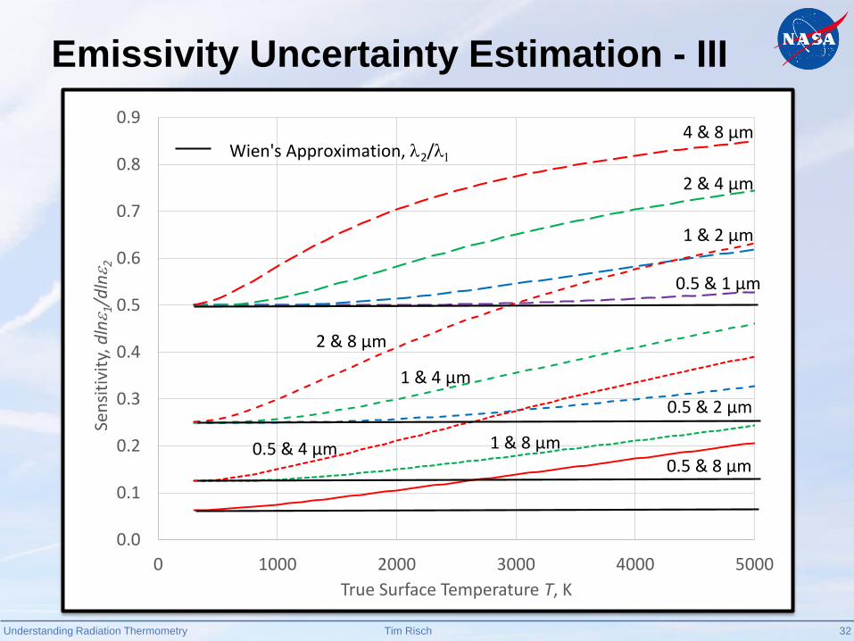
Emissivity Uncertainty Estimation - II

Unlike with temperature, the uncertainty in the computed emissivity decreases with increasing wavelength.

The error is approximately inversely proportional to the ratio of the two wavelengths.

Therefore emissivities derived from longer wavelength detectors have less uncertainty. However, since the emissivity is usually a strong function of wavelength, values at long wavelengths may or may not be useful if emissivities over the entire wavelength band are needed.


Emissivity Uncertainty Estimation - III

0.0

0.1

0.2

0.3

0.4

0.5

0.6

0.7

0.8

0.9

0 1000 2000 3000 4000 5000

Sen

siti

vity

, dln 1

/dln 2

True Surface Temperature T, K

0.5 & 1 µm

0.5 & 2 µm

0.5 & 4 µm0.5 & 8 µm

1 & 2 µm

1 & 4 µm

1 & 8 µm

2 & 8 µm

4 & 8 µm

2 & 4 µm

Wien's Approximation, 2/1


Example 8 - I

E8: A 0.53-m wavelength detector is used to determine the surface temperature. The measured equivalent blackbody temperature from this detector is 1,950 K and the emissivity is estimated to be 0.6 with an estimated uncertainty of 25%. What are the inferred emissivities and uncertainties at 1.0 m and 5.8 m if detectors at both wavelengths indicate equivalent blackbody temperatures of 1,740 K?


Example 8 - II

A8: The true surface temperature using Equation 13 and routine bb_tst is:

𝑇 = 14,388 m−K 0.53 𝜇m

ln 0.8 ∙ 𝑒 14,388 m−K 0.53 m∙ 1,950 K − 1 + 1= 2,024 K

The emissivity at 1.0 m using Equation 15 and routine bb_emiss is:

𝜀𝜆2 =𝑒 14,388 𝜇m−K 1.0 𝜇m−2,024 K − 1

𝑒 14,388 𝜇m−K 1.0 𝜇m−1,740 K − 1= 0.313


Example 8 - II

The sensitivity to the emissivity at wavelength 2 based on the assumed emissivity at wavelength 1 using Equation 19 and routine bb_dlne2dlne1 is:

𝑑 ln 𝜀𝜆2𝑑 ln 𝜀𝜆1

=0.53 𝜇m

1.0 𝜇m∙𝑒 14,388 𝜇m−K 0.53 𝜇m ∙2,024 K − 1

𝑒 14,388 𝜇m−K 1.0 𝜇m ∙2,024 K − 1= 0.530

And the relative uncertainty in the emissivity is:

∆𝜀𝜆2𝜀𝜆2

=𝑑 ln 𝜀𝜆2𝑑 ln 𝜀𝜆1

∙∆𝜀𝜆2𝜀𝜆2

= 0.530 ∙ 25% = 13.3%

The emissivity at 5.8 m using routine bb_emiss is:

𝜀𝜆2 =𝑒 14,388 𝜇m−K 5.8 𝜇m−2,024 K − 1

𝑒 14,388 𝜇m−K 5.8 𝜇m−1,740 K − 1= 0.761


Example 8 - III

The sensitivity to the emissivity at wavelength 2 based on the assumed emissivity at wavelength 1 using routine bb_dlne2dlne1 is:


=0.53𝜇m

5.8𝜇m∙𝑒 14,388 𝜇m−K 0.53𝜇m ∙2,024 K − 1

𝑒 14,388 𝜇m−K 5.8𝜇m ∙2,024 K − 1= 0.129

And the relative uncertainty in the emissivity is:

∆𝜀𝜆2𝜀𝜆2

=𝑑 ln 𝜀𝜆2𝑑 ln 𝜀𝜆1

∙∆𝜀𝜆2𝜀𝜆2

= 0.129 ∙ 25% = 3.2%

Note that the emissivity uncertainty at 5.8 𝜇m is four times less than at 1𝜇m.


Rule 2

The uncertainty in the spectral emissivity at a given wavelength decreases approximately inversely with the wavelength that is used.


Method 2 – Ratio method - I

Make measurements 𝑇𝜆1and 𝑇𝜆2with detectors at two different

wavelengths 𝜆1 and 𝜆2. Assume a ratio for the spectral emissivities at the two wavelengths ε𝑟 (could be 1) and then calculate the true temperature 𝑇 by solving the following:

and then calculate the individual emissivities from:

ε𝑟 =ε𝜆1ε𝜆2

= 𝑖𝑏,𝜆1 𝑇𝜆1 𝑖𝑏,𝜆1 𝑇

𝑖𝑏,𝜆2 𝑇𝜆2 𝑖𝑏,𝜆2 𝑇(21)

𝜀𝜆1 = 𝑖𝑏,𝜆1 𝑇𝜆1 𝑖𝑏,𝜆1 𝑇

𝜀𝜆2 = 𝑖𝑏,𝜆2 𝑇𝜆2 𝑖𝑏,𝜆2 𝑇(22)


Method 2 – Ratio method - II

If Wien’s approximation is valid, the approximate solution for the true temperature 𝑇 can be calculated directly by:

where Λ is an equivalent wavelength

and 𝑇𝑟 is the ratio temperature, the temperature of an equivalent blackbody having the same ratio of spectral radiances at the two specified wavelengths as that of the target.

1

𝑇=

1

𝑇𝑟−

𝛬

𝐶2ln 𝜀𝑟 (23)

Λ =𝜆1𝜆2

𝜆2 − 𝜆1(24)

1

𝑇𝑟=

Λ

𝜆1𝑇𝜆1+

Λ

𝜆2𝑇𝜆2(25)


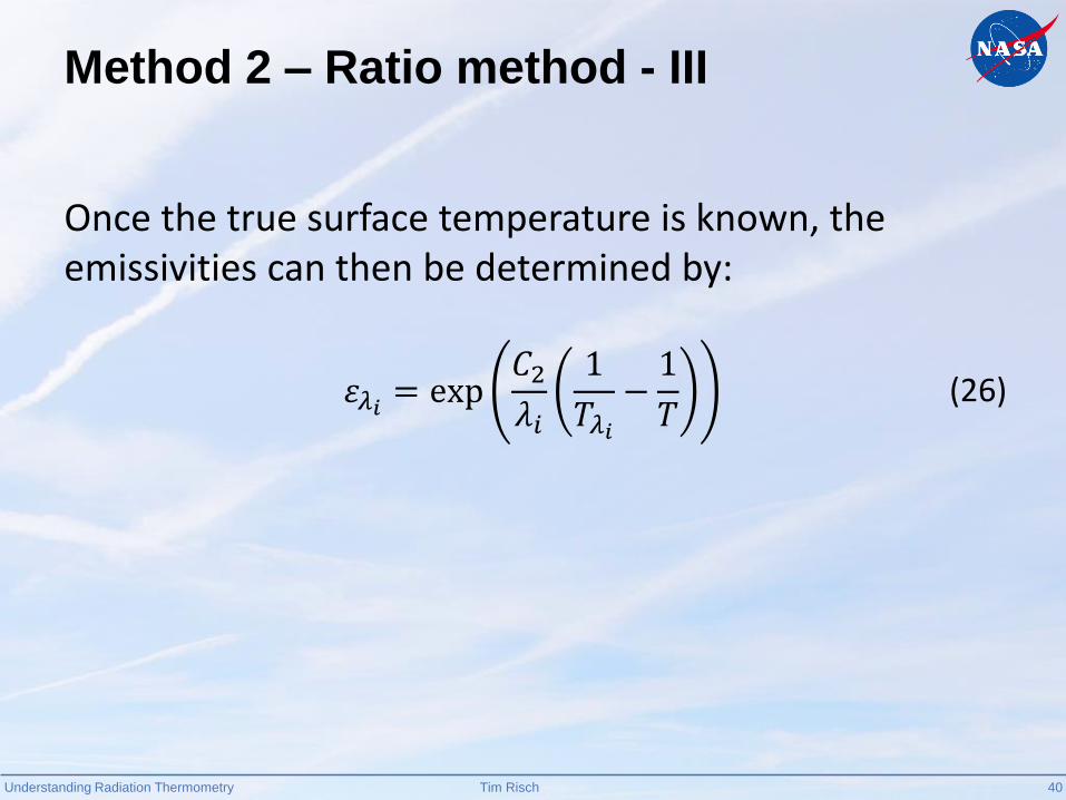
Method 2 – Ratio method - III

Once the true surface temperature is known, the emissivities can then be determined by:

𝜀𝜆𝑖 = exp𝐶2𝜆𝑖

1

𝑇𝜆𝑖−1

𝑇(26)


Ratio Method Observations

For an emissivity ratio of 1, the calculated ratio temperature of the instrument is the true surface temperature.

The equivalent wavelength can be much greater than either of the two individual wavelengths when the difference between the two wavelengths is small.

As the difference between the two wavelengths increases, the value of the equivalent wavelength approaches 1.

For Wien’s approximation to be valid, the wavelength temperature product of the two individual detectors need to be small, not the product of the equivalent temperature and the effective wavelength.

Equation 22 for the true surface temperature is identical to the equation for surface temperature in the spectral method (Equation 14) with the effective wavelength replacing the single wavelength and the ratio temperature replacing the single detector temperature.


Example 9 - I

E9: For a two-band radiation thermometer with detector wavelengths at 0.5 and 0.6 m, what are the true surface temperature and the spectral emissivities when the measured equivalent blackbody temperatures at the two wavelengths are 2,800 and 2,750 K, respectively and an emissivity ratio of 0.9 is assumed?


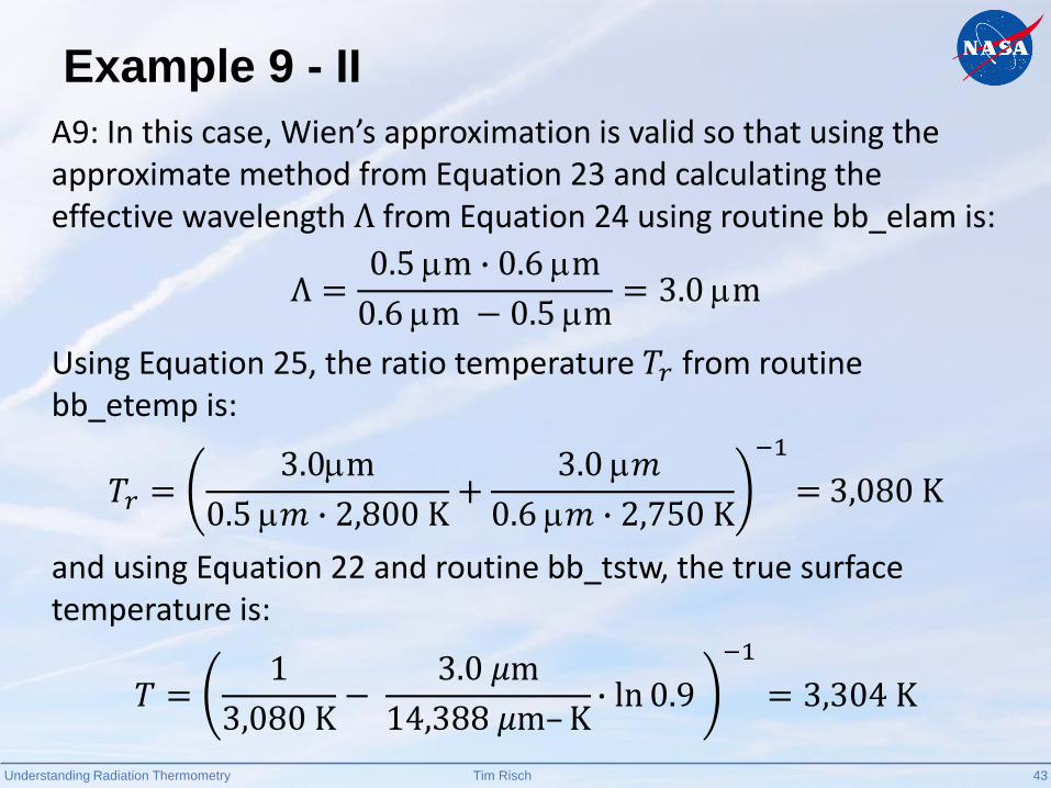
Example 9 - II

A9: In this case, Wien’s approximation is valid so that using the approximate method from Equation 23 and calculating the effective wavelength Λ from Equation 24 using routine bb_elam is:

Λ =0.5 m ∙ 0.6 m

0.6 m − 0.5 m= 3.0 m

Using Equation 25, the ratio temperature 𝑇𝑟 from routine bb_etemp is:

𝑇𝑟 =3.0m

0.5 𝑚 ∙ 2,800 K+

3.0 𝑚

0.6 𝑚 ∙ 2,750 K

−1

= 3,080 K

and using Equation 22 and routine bb_tstw, the true surface temperature is:

𝑇 =1

3,080 K−

3.0 𝜇m

14,388 𝜇m–K∙ ln 0.9

−1

= 3,304 K


Example 9 - III

Knowing the individual measured detector temperatures and the surface temperature, the emissivities are determined using Equation 18 and routine bb_emiss:

𝜀𝜆1 =𝑒14,388 𝜇m–K/0.5 μm∙3,304 K − 1

𝑒14,388 𝜇m–K/0.5 μm∙2,800 K − 1= 0.209

𝜀𝜆2 =𝑒14,388 𝜇m–K/0.6 μm∙3,304 K − 1

𝑒14,388 𝜇m–K/0.6 μm∙2,750 K − 1= 0.232

So that 𝜀𝜆1 𝜀𝜆2 = 0.9, consistent with our initial assumption.


Ratio Method Sensitivities

The sensitivity of the true surface temperature to the emissivity ratio can be calculated for the case where Planck’s law is valid by differentiating equation 17. This is:

When Wien’s approximation is valid, then the sensitivity can be easily determined utilizing the similarity to the spectral method as discussed before. The sensitivity then becomes:

𝑑 ln 𝑇

𝑑 ln 𝜀𝜆𝑖=Λ𝑇

𝐶2(28)

𝑑 ln𝑇

𝑑 ln 𝜀𝑟=

𝑒 𝐶2 𝜆1𝑇 −1 ∙ 𝑒 𝐶2 𝜆2𝑇 −1

𝐶2𝑒 𝐶2 𝜆2𝑇

𝜆2𝑇∙ 𝑒 −𝐶2 𝜆1𝑇 −1 −

𝐶2𝑒 𝐶2 𝜆1𝑇

𝜆1𝑇∙ 𝑒 𝐶2 𝜆2𝑇 −1

(27)


Example 10 - I

E10: For the same conditions as Example 9, what would the error in the true surface temperature be if an assumed emissivity ratio of 1.0 was used but the actual ratio of the surface emissivities was 0.9?


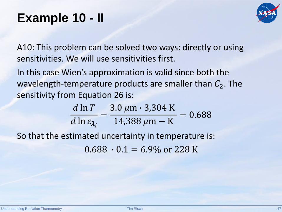
Example 10 - II

A10: This problem can be solved two ways: directly or using sensitivities. We will use sensitivities first.

In this case Wien’s approximation is valid since both the wavelength-temperature products are smaller than 𝐶2. The sensitivity from Equation 26 is:

𝑑 ln 𝑇

𝑑 ln 𝜀𝜆𝑖=3.0 𝜇m ∙ 3,304 K

14,388 𝜇m − K= 0.688

So that the estimated uncertainty in temperature is:

0.688 ∙ 0.1 = 6.9% or 228 K


Example 10 - III

Rather than using sensitivities, we can calculate the difference directly:

For an emissivity of 1.0, the true surface temperature is just the ratio temperature, or 3080 K. Therefore, the error is:

3080 K − 3,304 K = 224 K

almost exactly equal to the linear approximation using sensitivities.


Example 11 - I

E11: For a two-band radiation thermometer with detector wavelengths at 4.0 and 8.0 m, what is the error introduced when an emissivity ratio of 1.0 is assumed, when in fact the emissivity ratio of the sample has a ratio of 0.9? Assume the measured spectral temperatures at the two wavelengths are 2,800 and 2,750 K, the same as in Problem 9.


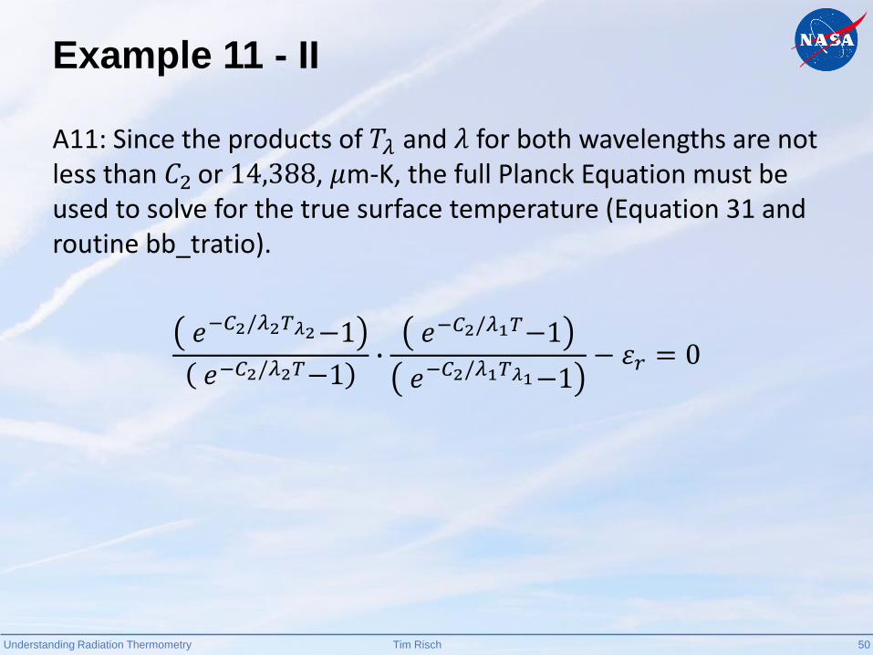
Example 11 - II

A11: Since the products of 𝑇𝜆 and 𝜆 for both wavelengths are not less than 𝐶2 or 14,388, 𝜇m-K, the full Planck Equation must be used to solve for the true surface temperature (Equation 31 and routine bb_tratio).

𝑒−𝐶2/𝜆2𝑇𝜆2−1

𝑒−𝐶2/𝜆2𝑇−1∙

𝑒−𝐶2/𝜆1𝑇−1

𝑒−𝐶2/𝜆1𝑇𝜆1−1− 𝜀𝑟 = 0


Example 11 - III

The calculated values for true temperatures are:

𝜀𝑟 = 0.9, 𝑇 = 4,118 K

𝜀𝑟 = 1.0, 𝑇 = 2,974 K

The difference is 1,144 K!

This example points out the large error using long wavelengths and the need to use short wavelengths whenever possible.


Example 11 - IV

The sensitivity of the emissivity ratio to surface temperature is (Equation 27):

𝑑 ln 𝜀𝑟𝑑 ln𝑇

=1

𝑇∙𝑒 𝐶2 𝜆2𝑇 − 1

𝑒 𝐶2 𝜆1𝑇 − 1∙

𝐶2𝜆2𝑇

𝑒𝐶2𝜆2𝑇

𝑒 𝐶2 𝜆1𝑇 − 1

𝑒 𝐶2 𝜆2𝑇 − 1 2−

𝐶2𝜆1𝑇

𝑒 𝐶2 𝜆1𝑇

𝑒 𝐶2 𝜆2𝑇 − 1

Since the temperature change is so great, linear sensitivities extrapolated from one point will not be accurate.

However, the calculated sensitivities are:

𝜀𝑟 = 0.9,𝑑 ln 𝑇

𝑑 ln 𝜀𝑟= −3.77

𝜀𝑟 = 1.0,𝑑 ln 𝑇

𝑑 ln 𝜀𝑟= −2.56


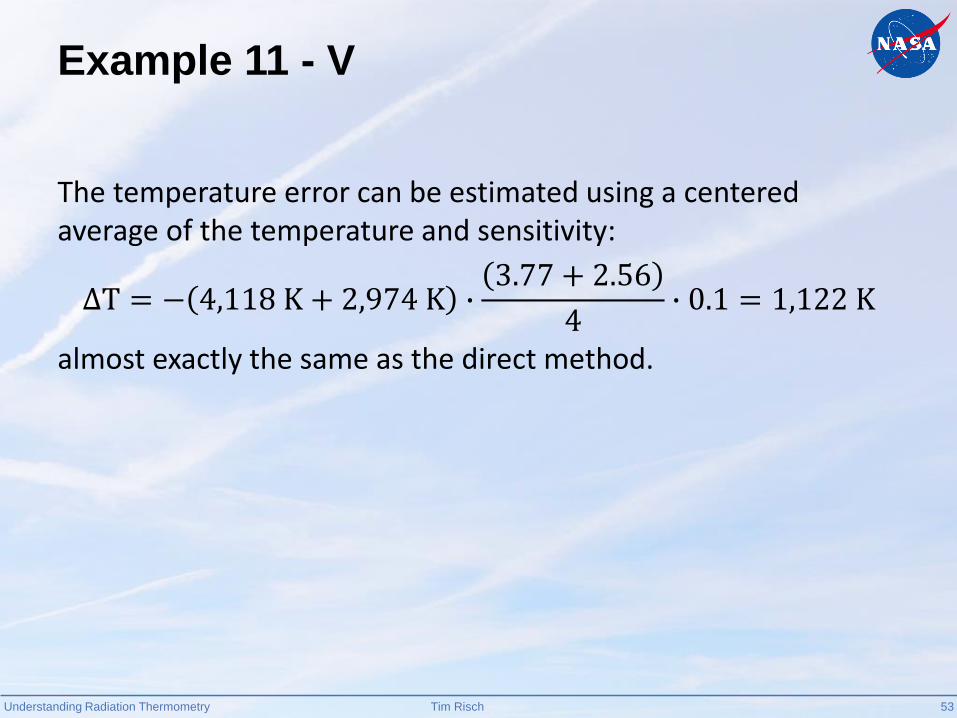
Example 11 - V

The temperature error can be estimated using a centered average of the temperature and sensitivity:

∆T = − 4,118 K + 2,974 K ∙3.77 + 2.56

4∙ 0.1 = 1,122 K

almost exactly the same as the direct method.


Further Observations

The selection of the optimal detector wavelengths for the ratio method is based upon two competing factors. As difference in the two detector wavelengths approaches zero the value of the effective wavelength goes to infinity and therefore tends to drive the temperature uncertainty higher. However, at the same time the smaller the difference in wavelengths makes the estimation of the emissivity ratio more accurate and therefore drives the temperature uncertainty lower.


Rule 3

The optimal detector wavelengths for the ratio method are based on the two competing factors: 1) the need to keep the wavelength difference small to ensure an accurate assumed ratio, but 2) not too small that the effective wavelength increases and becomes too large.


Multispectral Methods - I

Multispectral methods are an extension of the ratio method where a larger number of detectors are used.

Multiple measurements are then used to perform a best fit to single temperature and wavelength relationship.

The emissivity relationship can be a constant value or some other more complex function such as a polynomial.


Multispectral Methods - II

Advantages

› Large number of detectors reduces noise and averages errors inherent in measurements

Disadvantages

› Requires more complex hardware

› Multiple detectors increases data collection requirements and requires increased processing

› Data may not provide an identifiably unique solution unless a large number of measurements are made


Multispectral Hardware Utilizing Dispersive

Spectrometer and Silicon Array Detector

Focusing Mirrors

Grating

Array Detector

Entrance Slit32-Channel Array Silicon Detector


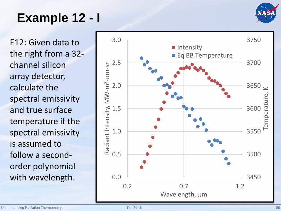
Example 12 - I

E12: Given data to the right from a 32-channel silicon array detector, calculate the spectral emissivity and true surface temperature if the spectral emissivity is assumed to follow a second-order polynomial with wavelength. 3450

3500

3550

3600

3650

3700

3750

0.0

0.5

1.0

1.5

2.0

2.5

3.0

0.2 0.7 1.2

Tem

per

atu

re, K

Rad

ian

t In

ten

sity

, MW

-m2-

m-s

r

Wavelength, m

IntensityEq BB Temperature


Example 12 - II

A12: The solution requires that we find values for 𝑇, 𝑎0, 𝑎1, and 𝑎2 that minimize the function 𝑓:

where𝑓 =

𝑖

𝑛

𝜀𝜆𝑖 ∙ 𝑖𝑏,𝜆𝑖(𝑇) − 𝑖𝜆𝑖(𝑇𝜆𝑖)2

(29)

𝜀 = 𝑎2𝜆2 + 𝑎1𝜆 + 𝑎0 (30)


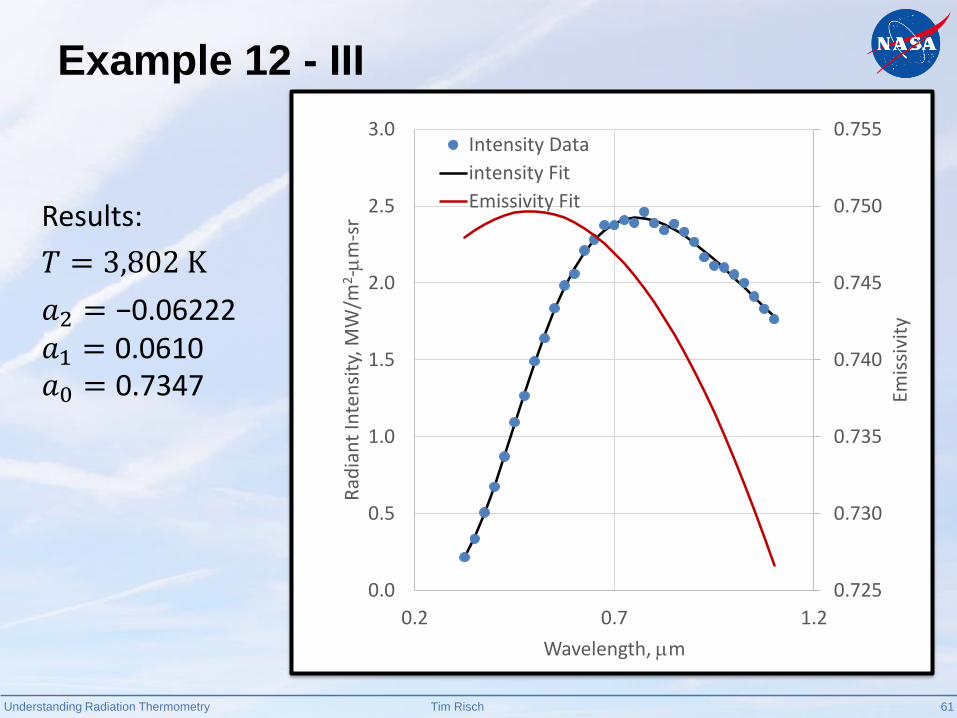
Results:

𝑇 = 3,802 K

𝑎2 = −0.06222𝑎1 = 0.0610𝑎0 = 0.7347

Example 12 - III

0.725

0.730

0.735

0.740

0.745

0.750

0.755

0.0

0.5

1.0

1.5

2.0

2.5

3.0

0.2 0.7 1.2

Emis

sivi

ty

Rad

ian

t In

ten

sity

, MW

/m2-

m-s

r

Wavelength, m

Intensity Data

intensity Fit

Emissivity Fit


Wide-Bandwidth Detectors

“The laws of light and of heat translate each other;—so do the laws of sound and colour; and so galvanism, electricity and magnetism are varied forms of this selfsame energy.”— Ralph Waldo Emerson


Wide-Bandwidth Detectors - I

Up until now, we have considered only narrow-band detectors, ones in which the wavelength band has been limited

Sometime, using wide-band detectors prove to be an advantage

However, using wide-band detectors is more difficult and requires additional understanding to properly interpret the measured data


Wide-Bandwidth Detectors - II

Advantages

› Provide a higher signal since the signal is measured over a wider band

› Require less hardware since the wavelength limiting device is eliminated

Disadvantages

› Introduces non-linearities in the calibration because the blackbody intensity varies with wavelength and the response of the detector is not uniform across all wavelengths

› Makes data reduction and analysis more complex


Wide-Bandwidth Detectors - III

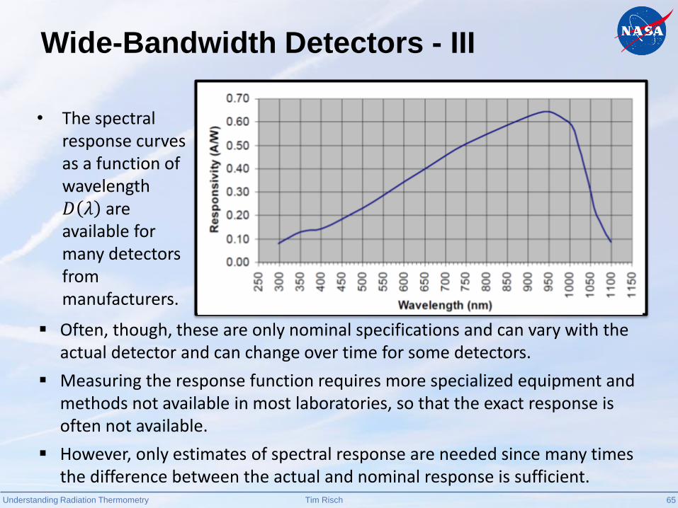
• The spectral response curves as a function of wavelength 𝐷 𝜆 are available for many detectors from manufacturers.

Often, though, these are only nominal specifications and can vary with the actual detector and can change over time for some detectors.

Measuring the response function requires more specialized equipment and methods not available in most laboratories, so that the exact response is often not available.

However, only estimates of spectral response are needed since many times the difference between the actual and nominal response is sufficient.


Wide-Bandwidth Detectors - III

Non-linearities in the calibration are introduced because the measured signal is the net product of the detector response multiplied by the blackbody emission intensity.

× =

Wavelength Wavelength Wavelength

Det

ecto

r R

esp

on

se

Bla

ckb

od

yIn

ten

sity

Net

Mea

sure

men

t


Wide-Bandwidth Detectors - IV

Using a wide-band detector can then require relating the integral of the blackbody function 𝑖𝑏,𝜆 , 𝑇 multiplied by the detector response 𝐷 across the bandwidth

When measuring materials with emissivities that vary over wavelength, the data analysis becomes even more complex and requires the inclusion of the emissivity 𝜀() with

wavelength

So that the measured signal becomes a function of the:

And not just 𝑖𝑏,𝜆 , 𝑇 .

𝑙

𝑢𝐷 ∙ 𝜀() ∙ 𝑖𝑏,𝜆 , 𝑇 𝑑 (31)


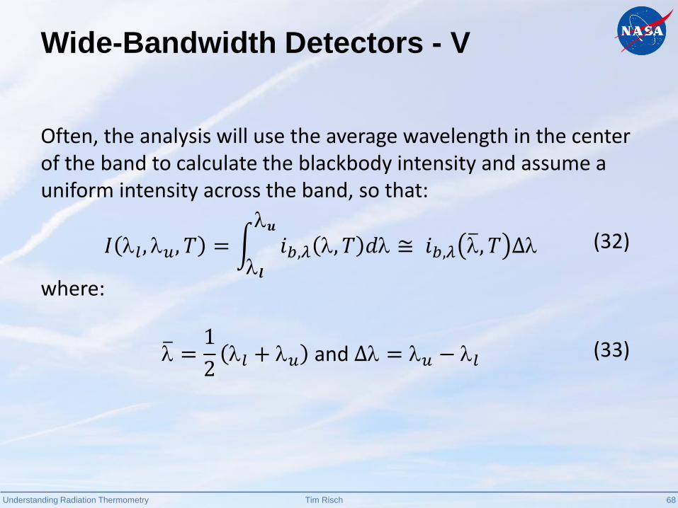
Wide-Bandwidth Detectors - V

Often, the analysis will use the average wavelength in the center of the band to calculate the blackbody intensity and assume a uniform intensity across the band, so that:

where:

=1

2𝑙 + 𝑢 and ∆ = 𝑢 − 𝑙 (33)

𝐼 𝑙 , 𝑢, 𝑇 = 𝒍

𝒖𝑖𝑏,𝜆 , 𝑇 𝑑 ≅ 𝑖𝑏,𝜆 , 𝑇 ∆ (32)


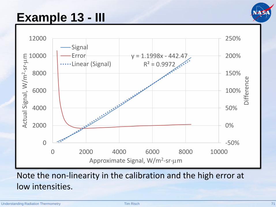
Example 13 - I

E13: What is the non-linearity introduced by averaging the response of a detector covering the range of 1 to 4 m at temperatures between 600 to 1100 K? Assume a uniform spectral response function.


Example 13 - II

A13: The problem requires that we compare:

𝑙

𝑢𝑖𝑏,𝜆 , 𝑇 𝑑

to:

𝑖𝑏,𝜆 , 𝑇 ∆

where

=1

2𝑙 + 𝑢 and ∆ = 𝑢 − 𝑙

So = 2.5 m and ∆ = 3.0 m. The comparison is shown on the following page.


Example 13 - III

Note the non-linearity in the calibration and the high error at low intensities.

y = 1.1998x - 442.47R² = 0.9972

-50%

0%

50%

100%

150%

200%

250%

0

2000

4000

6000

8000

10000

12000

0 2000 4000 6000 8000 10000

Approximate Signal, W/m2-sr-m

Dif

fere

nce

Act

ual

Sig

nal

, W/m

2-s

r-

m

SignalErrorLinear (Signal)


Example 14

E14: What is the non-linearity introduced by averaging the response of a detector covering the range of 0.25 to 1.05 m at temperatures between 2000 to 3000 K? Assume a linearly increasing detector spectral response function as shown below:

0

0.2

0.4

0.6

0.8

1

1.2

0 0.5 1 1.5

Det

ecto

r R

esp

on

se

Wavelength, m


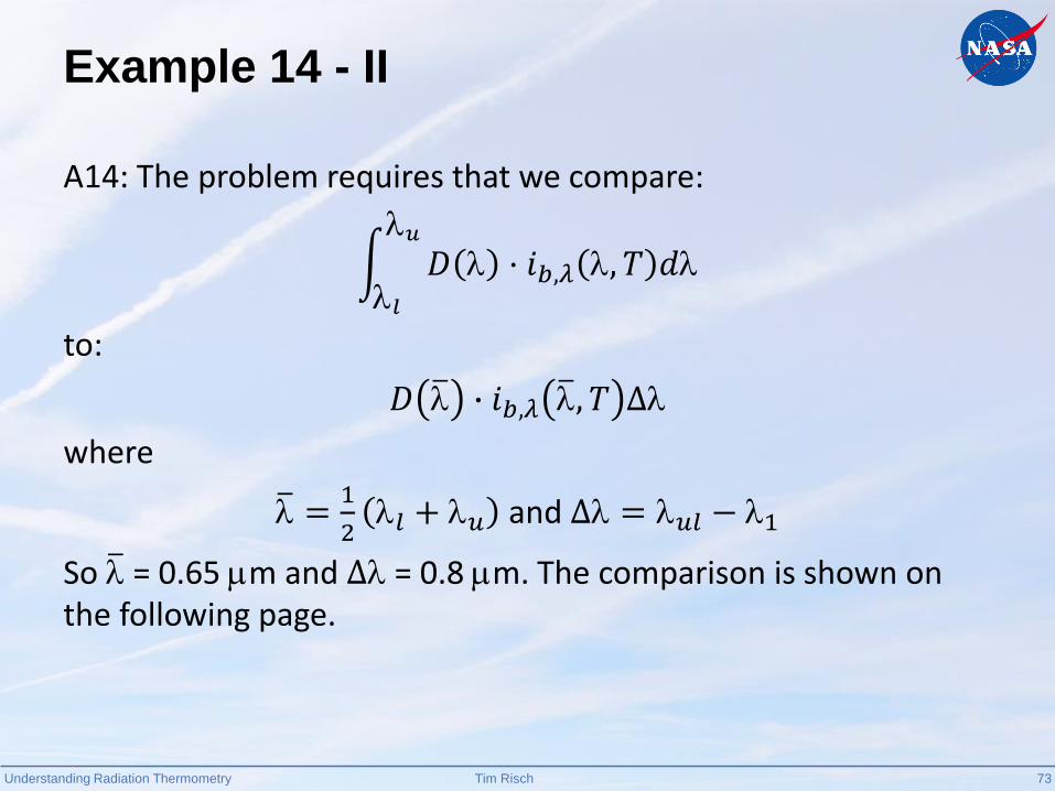
Example 14 - II

A14: The problem requires that we compare:

𝑙

𝑢𝐷 · 𝑖𝑏,𝜆 , 𝑇 𝑑

to:

𝐷 ∙ 𝑖𝑏,𝜆 , 𝑇 ∆

where

=1

2𝑙 + 𝑢 and ∆ = 𝑢𝑙 − 1

So = 0.65 m and ∆ = 0.8 m. The comparison is shown on the following page.


Example 14 -III

The result is similar to problem 13. Again note the non-linearity in the calibration and the high error at low intensities.

y = 0.6531x - 7737.6R² = 0.9961

-10%

-5%

0%

5%

10%

15%

20%

25%

30%

0

10000

20000

30000

40000

50000

60000

70000

0 50000 100000 150000

Approximate Signal, W/m2-sr-m

Dif

fere

nce

Act

ual

Sig

nal

, W/m

2-s

r-

m

SignalErrorLinear (Signal)


When measurements are made of materials with emissivities that vary over wavelength, the data analysis becomes even more complex and requires the inclusion of the emissivity with wavelength:

𝑙

𝑢𝐷(𝜆) ∙ 𝜀() ∙ (𝑖𝑏,𝜆 , 𝑇 𝑑 = 𝑖(𝒍, 𝑢, 𝑇) (33)

Wide-Bandwidth Detectors - V


When the two or more detectors are used, the relationships for the unknown temperatures and spectral emissivities involve integrals over the wavelength band.

Similar to the narrow-band ratio method, we can devise an analogous way to determine temperature and a wavelength-averaged emissivity.

Wide-Bandwidth Detectors - VI


For two, wide-band detectors measuring equivalent blackbody temperatures of 𝑇1 and 𝑇2, we can define an equivalent ratio method where we solve the following:

Where ε1 and ε2 are wavelength average emissivities. The next example will demonstrate this method.

ε𝑟 = ε1 ε2= 𝜆1𝒍𝜆1𝒖𝐷1(𝜆)(𝑖𝑏,𝜆 𝑇1 𝑑𝜆

𝜆1𝒍𝜆1𝒖𝐷1(𝜆)(𝑖𝑏,𝜆 𝑇 𝑑𝜆

∙ 𝜆2𝒍𝜆2𝒖𝐷2(𝜆)(𝑖𝑏,𝜆 𝑇 𝑑𝜆

𝜆2𝒍𝜆2𝒖𝐷2(𝜆)(𝑖𝑏,𝜆 𝑇2 𝑑𝜆

(34)

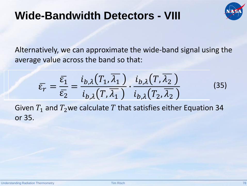
Wide-Bandwidth Detectors - VII


Alternatively, we can approximate the wide-band signal using the average value across the band so that:

Given 𝑇1 and 𝑇2we calculate 𝑇 that satisfies either Equation 34 or 35.

ε𝑟 = ε1 ε2=𝑖𝑏,𝜆 𝑇1, 𝜆1

𝑖𝑏,𝜆 𝑇, 𝜆1∙𝑖𝑏,𝜆 𝑇, 𝜆2

𝑖𝑏,𝜆 𝑇2, 𝜆2(35)

Wide-Bandwidth Detectors - VIII


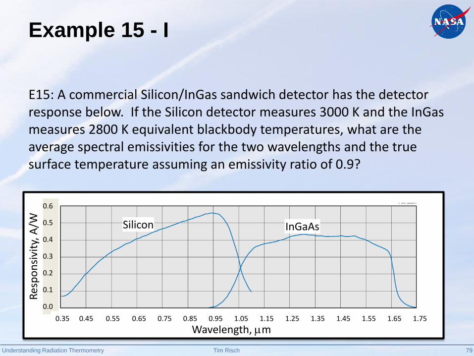
E15: A commercial Silicon/InGas sandwich detector has the detector response below. If the Silicon detector measures 3000 K and the InGas measures 2800 K equivalent blackbody temperatures, what are the average spectral emissivities for the two wavelengths and the true surface temperature assuming an emissivity ratio of 0.9?

Example 15 - IR

esp

on

sivi

ty, A

/W

0.6

0.5

0.4

0.3

0.2

0.1

0.0

Wavelength, m0.35 0.45 0.55 0.65 0.75 0.85 0.95 1.05 1.15 1.25 1.35 1.45 1.55 1.65 1.75

Silicon InGaAs


Res

po

nsi

vity

, A/W

0.6

0.5

0.4

0.3

0.2

0.1

0.0

Wavelength, m

0.35 0.45 0.55 0.65 0.75 0.85 0.95 1.05 1.15 1.25 1.35 1.45 1.55 1.65 1.75

Silicon InGaAs

Example 15 - II

A15: We model the detector response function by the line segments below. The problem requires that we solve Equation 34 or 35 with ε𝑟 = 0.9 and 𝑇1 = 3000 K and 𝑇2 = 2800 K.


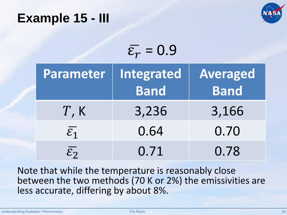
Example 15 - III

Parameter Integrated Band

Averaged Band

𝑇, K 3,236 3,166

𝜀1 0.64 0.70

𝜀2 0.71 0.78

Note that while the temperature is reasonably close between the two methods (70 K or 2%) the emissivities are less accurate, differing by about 8%.

ε𝑟 = 0.9


Example 16 - I

E16: This examples demonstrates the method of reducing data from wide-band detectors using effective, average wavelengths.

Consider a dual-band instrument with spectral bands covering 1 to 4.5 m and 2 to 13.5 m. The detector response functions are shown. The average detector wavelengths are 2.75 and 7 m. Using the average detector wavelengths, what is the surface temperature and what is the inferred emissivity assuming an emissivity ratio of 1?


Example 16 - II

Our example assumes a gray material which means that the spectral emissivity is

independent of wavelength. We assume the emissivity is equal to 0.65 and the true surface temperature is 3,000 K.

0

0.1

0.2

0.3

0.4

0.5

0.6

0.7

0.8

0.9

1

0 2 4 6 8 10 12 14

Emis

sivi

ty

Wavelength, m

𝜀 = 0.65


Example 16 - III

Using the function bb_tiibl, we can calculate what the measured equivalent blackbody temperatures 𝑇𝜆 would be by solving the following equation given the detector response functions 𝐷 𝜆 , the emissivity 𝜀 (independent of wavelength), and the spectral blackbody radiant intensity:

The calculated blackbody temperatures for detectors 1 and 2 are 2,589 and 2,426 K, respectively.

𝜀 𝜆𝑙

𝜆𝑢

𝐷 𝜆 𝑖𝑏,𝜆 𝑇 𝑑𝜆 = 𝜆𝑙

𝜆𝑢

𝐷 𝜆 𝑖𝑏,𝜆 𝑇𝜆 𝑑𝜆


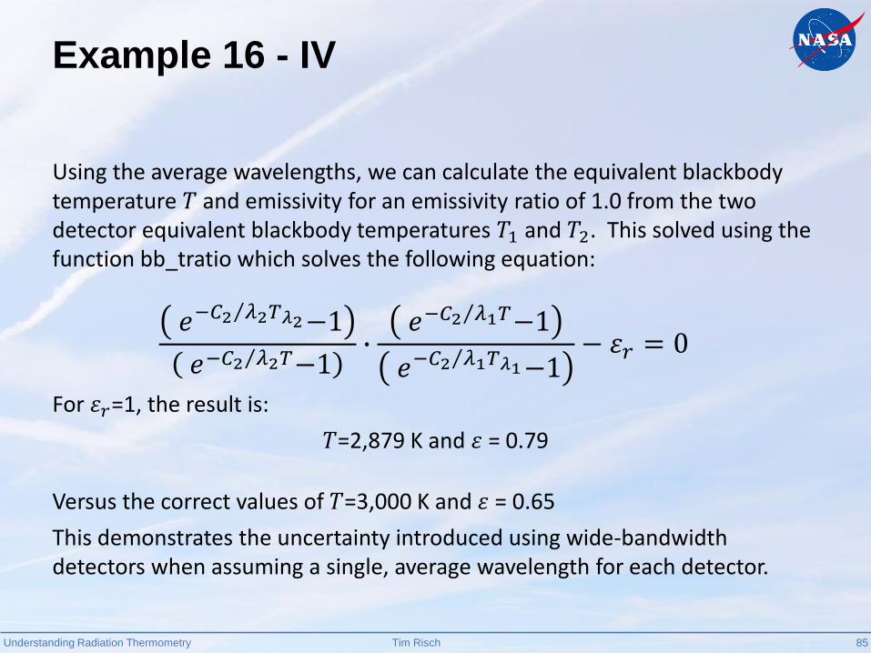
Example 16 - IV

Using the average wavelengths, we can calculate the equivalent blackbody temperature 𝑇 and emissivity for an emissivity ratio of 1.0 from the two detector equivalent blackbody temperatures 𝑇1 and 𝑇2. This solved using the function bb_tratio which solves the following equation:

For 𝜀𝑟=1, the result is:

𝑇=2,879 K and 𝜀 = 0.79

Versus the correct values of 𝑇=3,000 K and 𝜀 = 0.65

This demonstrates the uncertainty introduced using wide-bandwidth detectors when assuming a single, average wavelength for each detector.

𝑒 −𝐶2 𝜆2𝑇𝜆2−1

𝑒 −𝐶2 𝜆2𝑇−1∙

𝑒 −𝐶2 𝜆1𝑇−1

𝑒 −𝐶2 𝜆1𝑇𝜆1−1− 𝜀𝑟 = 0


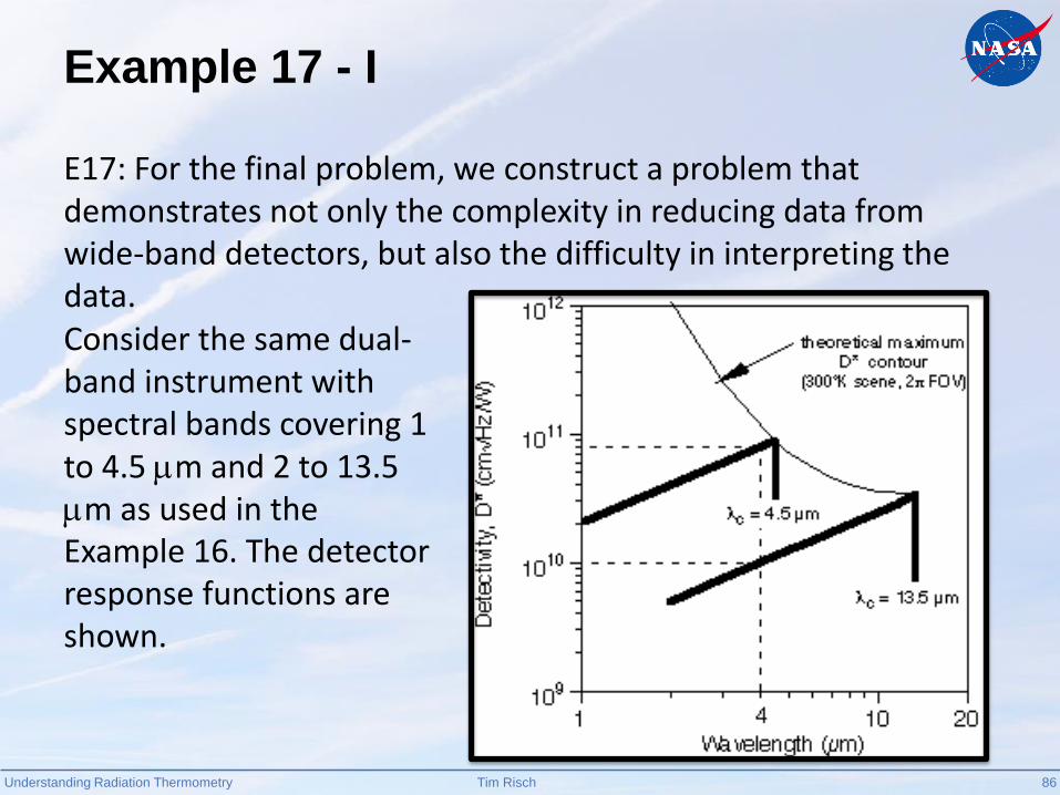
Example 17 - I

E17: For the final problem, we construct a problem that demonstrates not only the complexity in reducing data from wide-band detectors, but also the difficulty in interpreting the data.Consider the same dual-band instrument with spectral bands covering 1 to 4.5 m and 2 to 13.5 m as used in the Example 16. The detector response functions are shown.


Example 17 - II

The material has a spectral emissivity as a function of wavelength as shown. The true surface temperature is 3,000 K. Based on this, the calculated equivalent blackbody temperatures for the two detectors are 2,949 and 2,719 K respectively. If an emissivity ratio of 1 is assumed for the two detectors, what are the calculated true surface temperature and spectral emissivities?

0

0.2

0.4

0.6

0.8

1

0 2 4 6 8 10 12 14

Emis

sivi

ty

Wavelength, m

𝑑𝜀/𝑑𝜆=−0.025


Example 17 - III

For the given true surface temperature 𝑇, the calculated equivalent blackbody temperatures 𝑇𝜆𝒊for each detector can be

obtained by solving the following:

and as previously stated for detectors 1 and 2 are 2,941 and 2,841 K, respectively.

𝜆𝒊𝒍

𝜆𝒊𝒖

𝜖𝝀𝒊 𝜆 𝐷𝑖 𝜆 𝑖𝑏,𝜆 𝑇 𝑑𝜆 = 𝜆𝒊𝒍

𝜆𝒊𝒖

𝐷𝑖 𝜆 𝑖𝑏,𝜆 𝑇𝝀𝒊 𝑑𝜆


Example 17 - IV

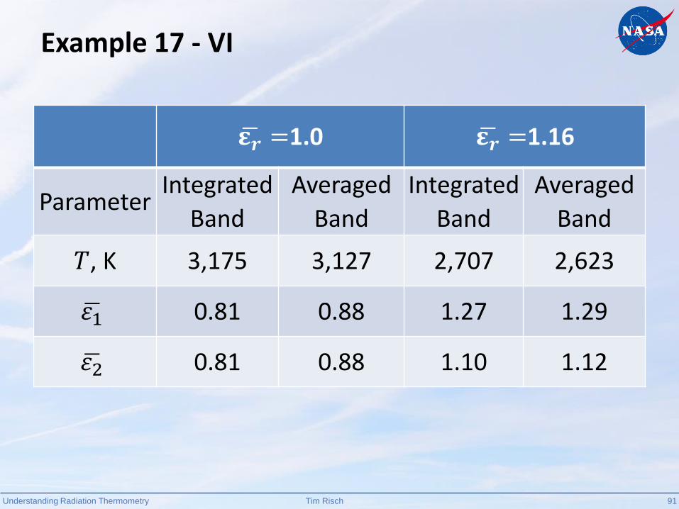
A17: Using the wide-band method with Equation 34 assuming an emissivity ratio ε𝑟 = 1, the calculated true surface temperature is 3,175 K with emissivities for the two detectors equal to 0.81 (routine bb_itratio). This is a 179-K error. If an emissivity ratio of 1.13 is assumed (equal to the ratio of the emissivities at the mean detector wavelengths), then a surface temperature of 2,707 K is calculated and the error in surface temperature increases to 294 K. The corresponding emissivities are calculated to be 1.27 and 1.10 for detector 1 and 2, respectively. These are not physically realistic.


Example 17 - V

If instead the equivalent narrow band assumption using Equation 34 with an emissivity ratio of 1.13 (routine bb_tratio) is used, the calculated true surface temperature is 2,622 K with emissivities for detector 1 and detector 2 being 1.29 and 1.12, respectively. Using an emissivity ratio of 1 results in a calculated temperature of 3,127 K and emissivities for both detectors equal to 0.88.

While the assumption of unity emissivity ratio comes closer to the correct surface temperature in both the wide-band and equivalent narrow-band methods, the result is fortuitous since the actual emissivity ratio across the two bands is not actually one.

The difficulty is that over such a wide range of wavelengths, it is difficult to choose the proper ratio since the wavelength dependence on spectral emissivity generally is not known.


Example 17 - VI

𝛆𝒓 =1.0 𝛆𝒓 =1.16

ParameterIntegrated

Band

Averaged

Band

Integrated

Band

Averaged

Band

𝑇, K 3,175 3,127 2,707 2,623

𝜀1 0.81 0.88 1.27 1.29

𝜀2 0.81 0.88 1.10 1.12


Rule 4

Unless other considerations dictate, avoid using wide-band detectors especially when accurate emissivities are needed.


Calibration

“Until you can measure something and express it in numbers, you have only the beginning of understanding.”– Lord Kelvin


Calibration

Detectors are calibrated against a source providing a known spectral intensity at a given wavelength.

However, it is often more convenient to express known calibration conditions in terms of an equivalent blackbody temperature, rather than a spectral intensity.

The calibrated spectral intensity and blackbody temperature are equivalent and can be used to determine the system response accounting for detector nonlinearities, transmission losses, and electrical gains.


Calibration Sources - I

Broadband Sources

› Blackbody Thermal Cavity – Near UV to IR

› Incandescent Lamp – Visible to Near IR

› Deuterium Arc Lamp – UV to Visible

Discrete Wavelength Sources

› Mercury Lamp

› Noble Gas (Neon, Argon, Krypton, Xenon) Lamp

Portable Blackbody Source

Deuterium Arc Lamp


Blackbody Source

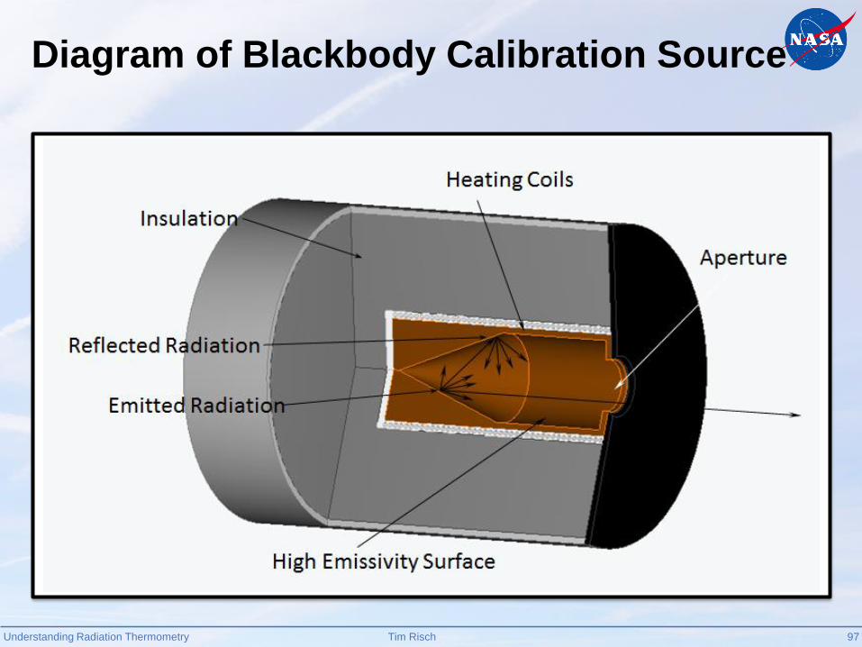
A blackbody calibration source is an especially convenient and accurate calibration source.

Recall, a perfect blackbody is an ideal emitter and absorbs all incident radiation regardless of the spectral character of directionality of the incident radiation.

This behavior is simulated using a heated cavity designed to have an effective near unity emissivity.

The specified calibration conditions can be determined by measuring the temperature of the cavity, rather than the absolute spectral radiance, like other sources.


Diagram of Blackbody Calibration Source


Calibration Sources - II

Resistively Heated, High-temperature Blackbody Furnace – 500 to 3000 C


s = 2.4208 × ib, + 0.023R² = 0.9926

0

5

10

15

20

25

30

35

0 5 10 15Si

gnal

, V

Radiant Intensity, W/m2-m-sr

= 0.656 m

𝑖_(𝑏,𝜆) (𝜆,𝑇)=1/𝜆5 · 𝐶1/(exp(𝐶_2/𝜆𝑇)−1)

Calibration Sources - III

0

2

4

6

8

10

12

14

1000 1100 1200 1300

Sign

al, V

Temperature, K

= 0.656 m

Blackbody calibration data for 0.656-m detector. The blackbody temperature was preset and the signal voltage measured. Plotting this versus the calculated radiant intensity produces a straight line of signal versus calculated intensity.


Calibration Uncertainty

All calibration sources have inherent error in the spectral intensity output.

For blackbody sources, this error manifests itself in the uncertainty in the cavity temperature measurement

Uncertainty in the cavity intensity propagates error just like the emissivity.

Uncertainty in cavity temperature can be calculated from the quantity 𝑑𝑇/𝑑𝜀.


Example 18 - I

E18: A blackbody source is estimated to have an uncertainty of 10 K and is used to perform a single-point calibration on two detectors, 1) a short-wavelength, 0.5-m detector and 2) a longer-wavelength 3 m detector. For an unknown material, the equivalent blackbody temperatures are measured to be 1,600 and 1,500 K, respectively. What is the value and the uncertainty in the derived emissivity at 3 m assuming the material has an emissivity of 0.8 0.1 at 0.5 m?


Example 18 - II

A17: The equivalent blackbody temperature from the measurement of the 0.5-m detector for 𝑇𝜆1 = 1,600 K and 𝜀𝜆1= 0.8 is:

The calculated emissivity at 3 m is:

Assuming the temperature errors in the two calibration measurements are uncorrelated and random, the total uncertainty in the emissivity will be:

where Δ𝑇𝜆1 = 10K and 𝜀𝜆1 = 0.1.

𝑇 =𝐶2𝜆1

∙1

ln 𝜀𝜆1 𝑒𝐶2/𝜆𝑇𝜆1 − 1 + 1= 1,604 𝐾

𝜀𝜆 =𝑒𝐶2/𝜆𝑇𝜆 − 1

𝑒𝐶2/𝜆𝑇 − 1= 0.78

𝜀𝜆2 =𝜕𝜀𝜆2𝜕𝑇𝜆1

Δ𝑇𝜆1

2

+𝜕𝜀𝜆2𝜕𝑇𝜆2

Δ𝑇𝜆2

2

+𝜕𝜀𝜆2𝜕𝜀𝜆1

Δ𝜀𝜆1

2


Example 18 - III

or, in terms of sensitivities:

evaluating terms gives:


=𝜆1𝜆2

∙𝑒 −𝐶2 𝜆1𝑇−1

𝑒− 𝐶2 𝜆2𝑇−1= 0.176

𝜀𝜆2𝜀𝜆2

=𝜕 ln 𝜀𝜆2𝜕 ln 𝜀𝜆1

𝜕 ln 𝜀𝜆1𝜕 ln𝑇𝜆1

Δ𝑇𝜆1𝑇𝜆1

2

+𝜕 ln 𝜀𝜆2𝜕 ln𝑇𝜆2

Δ𝑇𝜆2𝑇𝜆2

2

+𝜕 ln 𝜀𝜆2𝜕 ln 𝜀𝜆1

Δ𝜀𝜆1𝜀𝜆1

2

𝑑 ln 𝜀𝜆1𝑑 ln𝑇𝜆1

=𝐶2𝜆𝑇𝜆1

∙𝑒𝐶2/𝜆𝑇𝜆1

𝑒𝐶2/𝜆𝑇𝜆1 − 1= 18.0

𝑑 ln 𝜀𝜆2𝑑 ln𝑇𝜆2

=𝐶2𝜆𝑇𝜆2

∙𝑒𝐶2/𝜆𝑇𝜆2

𝑒𝐶2/𝜆𝑇𝜆2 − 1= 3.33


Example 18 - IV

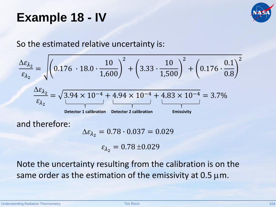
So the estimated relative uncertainty is:

and therefore:

Note the uncertainty resulting from the calibration is on the same order as the estimation of the emissivity at 0.5 m.

𝜀𝜆2𝜀𝜆2

= 0.176 ∙ 18.0 ∙10

1,600

2

+ 3.33 ∙10

1,500

2

+ 0.176 ∙0.1

0.8

2

𝜀𝜆2𝜀𝜆2

= 3.94 × 10−4 + 4.94 × 10−4 + 4.83 × 10−4 = 3.7%

𝜀𝜆2 = 0.78 0.029

𝜀𝜆2 = 0.78 ∙ 0.037 = 0.029

Detector 1 calibration Detector 2 calibration Emissivity


Closing

“If this fire determined by the sun, be received on the blackest known bodies, its heat will be long retain'd therein; and hence such bodies are the soonest and the strongest heated by the flame fire…”– Hermann BoerhaaveA New Method of Chemistry, 2nd edition (1741), 262


Closing - I

Radiation thermometry is a useful technique for measuring the temperature of bodies that cannot be readily measured by contact sensors.

It is important to understand the uncertainty in radiation thermometry measurements and choose the characteristics of the instrumentation and the measurement method accordingly.

The most accurate temperature measurements are obtained when using short wavelength detectors.

The uncertainty in the derived spectral emissivity at a given wavelength decreases approximately inversely with the wavelength that is used, and therefore longer wavelength detectors provide more accurate emissivity measurements.


Closing - II

Combining measurements of two or more detectors can allow the simultaneous determination of both the temperature and the emissivity.

However, the uncertainty in both the temperature and emissivity increase when the measurements of two detectors are combined.

Multi-spectral methods using a large number of detectors can often provide more accurate temperature and emissivity values over a wider range of wavelengths.

Prefer the use of narrow-band detectors over wide-band detectors unless other factors dictate.


Summary of Radiative Thermometry

Rules

Rule 1- When the emissivity is unknown and must be estimated, the most accurate surface temperature measurement is made when a detector with a wavelength as short as possible is used.

Rule 2 - The uncertainty in the spectral emissivity at a given wavelength decreases approximately inversely with the wavelength that is used.

Rule 3 - The optimal detector wavelengths for the ratio method are based on the two competing factors: 1) the need to keep the wavelength difference small to ensure an accurate assumed ratio, but 2) not too small that the effective wavelength increases and becomes too large.

Rule 4 -Unless other considerations dictate, avoid using wide-band detectors especially when accurate emissivities are needed.


For Further Reading1. Howell, J. R. , R. Siegel, and M. P. Mengüç, Thermal Radiation Heat Transfer, Fifth Edition,

Taylor & Francis, New York, 2010.

2. DeWitt, D. P. and G. D. Nutter, Theory and Practice of Radiation Thermometry, John Wiley and Sons, New York, 1988.

3. Rogalski, A., “History of Infrared Detectors”, Opto-Electron. Rev., 20 no. 3, pp 279-308, 2012.

4. Cupa, R. and A. Rogalski, “Performance limitations of photon and thermal infrared detectors”, Opto-Electr. Rev., 5, no. 4, 1997.

5. DeWitt, D. P. and R. Rondeau, “Measurement of Surface Temperatures and Spectral Emissivities During Laser Irradiation”, J. Thermophysics, Vol. 3, No. 2, pp. 153-159, April 1989.

6. Johnson, P. E., D. P. DeWitt and R. E. Taylor, “Method for Measuring High Temperature Spectral Emissivity of Nonconducting Materials”, AIAA Journal, Vol. 19, No. 1, pp. 113-120, January 1981. Also AIAA Paper, 79-1037.

7. Water, W.R., J. H. Walker, A. T. Hattenberg, “NBS Measurement Services: Radiance Temperature Calibration, National Bureau of Standards Special Publication 250-7, Oct., 1987. Available at: http://www.nist.gov/calibrations/upload/sp250-7.pdf

8. Ready, J., “Fundamentals of Photonics, Module 1.6 Optical Detectors and Human Vision”, SPIE, http://spie.org/Documents/Publications/00%20STEP%20Module%2006.pdf.

http://www.nist.gov/calibrations/upload/sp250-7.pdf


Acknowledgments

The author acknowledges funding for this work from the NASA NESC Passive Thermal Technical Committee. We are grateful for the comments and support provided by Mr. Steve Rickman, NESC Passive Thermal Technical Fellow and Mr. Daniel Ngyuen, Deputy of the Passive Thermal Technical Discipline Team. We also recognize the valuable comments and suggestions from Mr. Larry Hudson, Dr. William Ko, Mr. Chris Kostyk, and Mr. Matt Moholt of the Aerostructures Branch at NASA Armstrong Flight Research Center. Additional reviewers who provided many valuable comments also included Ms. Ruth Amundsen, Mr. Jentung Ku, Mr. David Gilmore, Mr. Richard Wear, and Mr. Duane Beach.


FINE