arX

iv:1

608.

0268

5v1

[as

tro-

ph.E

P] 9

Aug

201

6JOURNAL OF GEOPHYSICAL RESEARCH, VOL. ???, XXXX, DOI:10.1002/,

Understanding Jupiter’s Interior

Burkhard Militzer1,2, Francois Soubiran1, Sean M. Wahl1, William Hubbard3

1Department of Earth and Planetary Science, University of California, Berkeley, CA 94720, USA.2Department of Astronomy, University of California, Berkeley, CA 94720, USA.3Lunar and Planetary Laboratory, University of Arizona, Tucson, AZ 85721, USA.

Abstract. This article provides an overview of how models of giant planet interiors areconstructed. We review measurements from past space missions that provide constraintsfor the interior structure of Jupiter. We discuss typical three-layer interior models thatconsist of a dense central core and an inner metallic and an outer molecular hydrogen-helium layer. These models rely heavily on experiments, analytical theory, and first-principlecomputer simulations of hydrogen and helium to understand their behavior up to theextreme pressures ∼10 Mbar and temperatures ∼10 000 K. We review the various equa-tions of state used in Jupiter models and compare them with shock wave experiments.We discuss the possibility of helium rain, core erosion and double diffusive convectionmay have important consequences for the structure and evolution of giant planets. InJuly 2016 the Juno spacecraft entered orbit around Jupiter, promising high-precision mea-surements of the gravitational field that will allow us to test our understanding of gasgiant interiors better than ever before.

1. Introduction

In this article, we will provide a brief overview of howmodels for the interiors of giant planets are put together.While much of this discussion applies to all giant planets,this article will be focused on Jupiter in particular. We willreview results from space missions that visited the planetearlier and then we will discuss what we expect from theJuno mission presently in orbit around Jupiter.

All giant planet interior models rely on an equation ofstate that describes how materials behave under the extremepressure (∼10 Mbar) and temperature (∼10 000K) condi-tions in planetary interiors. So in section 3, we compare theresults from laboratory experiments, semi-analytical EOSmodels and ab initio simulations of dense hydrogen and ofhelium. In section 4, we review experimental and theoreticalpredictions for the properties of hydrogen-helium mixtures.We discuss ab initio simulations that focused on the questionwhether hydrogen-helium mixtures phase separate at highpressure, where hydrogen becomes a metallic fluid while he-lium remains in an insulating state. This process may leadto helium rain in the interior of giant planets, which hasbeen invoked by Stevenson and Salpeter [1977a, b] to ex-plain Saturn’s unusually large infrared emissions.

In section 5, we compare the prediction for Jupiter’stemperature-pressure profiles and discuss various interiormodels. In section 6, we compare adiabatic and super-adiabatic models, revisit the question of whether presentday Jupiter has dense central core and if a primordial corecould be partially or fully eroded.

2. Interior Constraints from Past SpaceMissions

Over the past 43 years Jupiter has been visited by ninespacecraft. Out of these missions the primary contributionsto our understanding of Jupiter’s interior were made by thePioneer 10 & 11 fly-bys, the Voyager 1 & 2 fly-bys and the

Copyright 2016 by the American Geophysical Union.0148-0227/16/$9.00

Galileo orbiter. In July 2016, the Juno spacecraft entered alow-periapse orbit, in order to provide the most precise mea-surement of Jupiter’s gravitational field to date, as well asbetter constraints on the composition of the outer envelope.

1960 1970 1980 1990 2000 2010 2020−100

−50

0

50

100

(J2

− 14

696.

43)

×106

1960 1970 1980 1990 2000 2010 2020−100

−80−60−40−20

02040

(J4

+ 5

96.0

5) ×

106

1960 1970 1980 1990 2000 2010 2020−30

−20

−10

0

10

20

(J6

− 35

.15)

×10

6

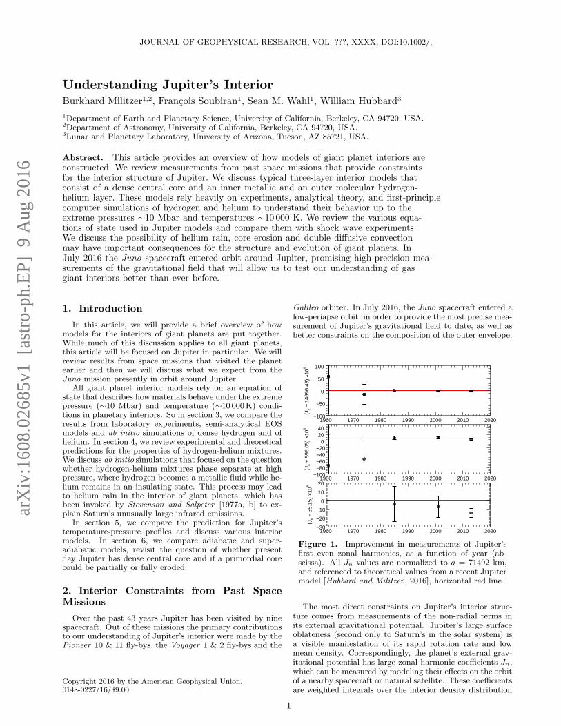
Figure 1. Improvement in measurements of Jupiter’sfirst even zonal harmonics, as a function of year (ab-scissa). All Jn values are normalized to a = 71492 km,and referenced to theoretical values from a recent Jupitermodel [Hubbard and Militzer , 2016], horizontal red line.

The most direct constraints on Jupiter’s interior struc-ture comes from measurements of the non-radial terms inits external gravitational potential. Jupiter’s large surfaceoblateness (second only to Saturn’s in the solar system) isa visible manifestation of its rapid rotation rate and lowmean density. Correspondingly, the planet’s external grav-itational potential has large zonal harmonic coefficients Jn,which can be measured by modeling their effects on the orbitof a nearby spacecraft or natural satellite. These coefficientsare weighted integrals over the interior density distribution

1

X - 2 MILITZER ET AL.: UNDERSTANDING JUPITER’S INTERIOR

ρ(r),

Jn = −2π

Man

∫

dr dµ ρ(r) rn+2 Pn(µ), (1)

where M is Jupiter’s mass, a is a normalizing radius (usu-ally taken to be the equatorial radius at a pressure of 1bar, 71492 km), µ = sinL (L is the planetocentric latitude),Pn(µ) are Legendre polynomials, and r is the radial distancefrom the planet’s center. To relate given values of Jn to in-terior structure, we assume that the planet is everywherein hydrostatic equilibrium in its rotating frame, and that aunique barotrope P = P (ρ) relates the pressure P and themass density ρ. Thus, a model of Jupiter using a barotropethat reproduces the external gravity terms is an acceptableone.

The J2 term in the harmonic expansion is mostly Jupiter’sinterior’s linear response to rotation, but higher-order termsJn arise entirely from nonlinear response, and require care-ful numerical modeling to properly test an assumed interiorbarotrope [Zharkov and Trubitsyn, 1978]. The higher-orderterms are difficult to measure at a significant distance fromJupiter since the gravitational potential contribution froma given zonal harmonic Jn varies as (a/r)n+1. Prior to thefirst spacecraft measurements at Jupiter in 1973, our onlyinformation about Jn came from ground-based observationsof satellite motions. Fig. 1 exhibits the dramatic improve-ment in measurements of the Jn over the last ∼50 years.

0 4 8 12 16 20 24Pressure [bar]

100

150

200

250

300

350

400

450

Tem

pera

ture

[K]

Galileo data

SCvH

0.9 1.0 1.1 1.2

160

165

170

175

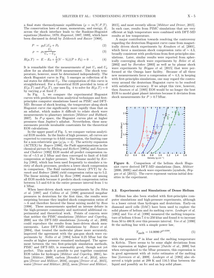
Figure 2. Comparison of Galileo entry probe T -P mea-surements [Galileo] with Saumon et al. [1995] EOS model.For the latter calculation, we assumed a dry adiabat withhelium mass fraction of 0.247 a starting from a tempera-ture of 166.1 K at 1 bar.

2.1. Pioneer and Voyager Missions

Pioneers 10 and 11 were the first spacecraft to reach thevicinity of Jupiter, in December 1973 and December 1974.These spacecraft executed hyperbolic flyby orbits with peri-apses at 2.8a and 1.6a respectively, permitting an improveddetermination of J2 and J4, but the signal from higher-order terms was not measurable. Voyagers 1 and 2 executedJupiter flybys in March 1979 and July 1979, with periapsesof 4.9a and 10.1a respectively. Thus, the Pioneer flybyswere more sensitive to terms above J2 [Campbell and Syn-nott , 1985].

2.2. Galileo Mission and Entry Probe

The Galileo spacecraft arrived at Jupiter in December1995, and remained in orbit around Jupiter for 8 years. Themain Galileo spacecraft did not make a large contribution to

improvements in measurements of Jupiter’s Jn, although itmade important measurements of the corresponding termsin the external gravity of the Galilean satellites.

Galileo’s most significant contribution to the understand-ing of Jupiter’s interior was deploying an entry probethat measured the structure and composition of Jupiter’snear-equatorial atmosphere to a maximum pressure of 22bar [Seiff et al., 1998]. The entry probe data are funda-mental as an initial condition for constraining the Jovianinterior barotrope. Conservatively estimated, the probe’ssensors were able to measure temperature with a precisionvarying from 0.1 K at 100 K to 1 K at 500 K [Magalhaeset al., 2002]. Seiff et al. [1998] inferred an uncertainty of lessthan 2% for probe’s pressure measurements by performingan a posteriori calibration that was needed because the tem-perature exceeded the original calibration range. Based onthese results, Seiff et al. [1998] fitted a dry adiabatic profilewith a temperature of 166.1 K at 1 bar, which we reproducedin Fig. 2 with a H-He isentrope derived from the Saumonet al. [1995] EOS model. We find a good agreement overallbetween the theoretical H-He isentrope and the measureddata but is a not a perfect match. For example there isdeviation of approximately 2 K at starting point of 1 bar.

The Galileo entry probe further constrained the com-position along the barotrope, showing the outer layers ofJupiter to have a composition that is not too different fromthat of the sun. The probe measured a helium mass frac-tion of Y = 0.23 and a mass fraction of heavier elementsof Z ≈ 0.017. The heavy element component was primar-ily comprised of the hydrides H2O, CH4, and NH3 [Wonget al., 2004]. It is important to note that the probe valueof Y is below the protosolar value of 0.274 [Lodders, 2003],providing evidence of helium sequestration in Jupiter’s in-terior. The probe’s measurement of a strong neon depletionwith respect to protosolar abundance was further evidenceof helium rain [Wilson and Militzer , 2010].

2.3. Combined Analysis from Past Missions

The next spacecraft to visit Jupiter was Ulysses, whichexecuted a flyby in February 1992 at 6.3a. Optimized tostudy the solar wind, Ulysses did not contribute significantlyto Jovian interior constraints. Subsequent encounters byCassini-Huygens in December 2000 and by New Horizonsbetween January and may 2007, did not afford opportunitiesto significantly improve measurements of Jupiter’s gravita-tional field.

During the long interval before the expected arrivalof the Juno orbiter in 2016, R. A. Jacobson [Jacobson,2001, 2003, 2013] has synthesized disparate data sets includ-ing Earth-based astrometry, satellite mutual eclipses and oc-cultations, and satellite eclipses by Jupiter, as well as space-craft data from Doppler tracking, radiometric range, very-long baseline interferometry, radio occultations, and opticalnavigation imaging from Pioneer 10 & 11, Voyager 1 &2, Ulysses, Galileo, and Cassini. More recent data pointsshown in Fig. 1 reflect this work.

2.4. Juno Mission

The Juno spacecraft, launched in 2011 and inserted inJupiter’s orbit on July 4, 2016, is optimized for measure-ments to constrain Jupiter’s interior structure. More than20 polar orbits with 14-day periods and perijoves at ∼ 1.07awill be devoted to X- and Ka-band measurements of space-craft motions in Jupiter’s gravity potential, with an ex-pected line-of-sight velocity precision ∼ 2µm/s. Terms inJupiter’s gravitational potential to ∼J10 should be measur-able, along with Jupiter’s second-degree tidal response to itsnearest large satellites. Predicted values of Jupiter’s J2, J4,and J6 are shown in Fig. 1; predictions of J8 and J10 are

MILITZER ET AL.: UNDERSTANDING JUPITER’S INTERIOR X - 3

Helium

droplets

Helium-poor

envelope

Layer of hydrogen-

helium immiscibility

Metallic hydrogen

(helium rich)

Rocky core

Molecular hydrogen

(helium depleted)

0.0

0.2

0.4

0.6

0.8

1.0

Fract

ional equato

rial ra

diu

s R/R

J

Rocky core

Metallic hydrogen

Heliu

m rain

layer

Mole

cula

r hydro

gen

0.0 0.2 0.4 0.6 0.8 1.0Fractional mass M(R)/MJ

0

10

20

30

40

50

60

70

Pre

ssure

(M

bar)

Figure 3. The upper diagram shows a model of Jupiter’sinterior with the hydrogen-helium immiscibility layer.Lower two diagrams show the fractional radius and pres-sure as a function of fractional mass according to Hubbardand Militzer [2016].

also published [Hubbard and Militzer , 2016]. Predicted val-ues of Jupiter’s tidal Love numbers [Wahl et al., 2016a, b] areavailable for comparison with the tidal measurements. Theprecision of predictions and expected measurements is suchthat relative discrepancies at the level of ∼ 10−7 would bedetectable. Gravity anomalies attributable to Jovian inte-rior dynamics, apart from purely hydrostatic response, mayproduce a detectable signal [Kaspi and Galanti , 2016].

Over the expected mission lifetime of ∼20 months, asufficient arc of the angular precession of Jupiter’s spinaxis should be measurable to yield a meaningful result forJupiter’s spin angular momentum, L = Cω, where C isJupiter’s axial moment of inertia and ω is the spin rate.If the relevant ω is the well-known and stable value forJupiter’s magnetic field, virtually any interior model fittedto J2 predicts C = 0.26Ma2 [Hubbard and Militzer , 2016].Measurement of an L significantly different from the valueimplied by Jupiter’s magnetic field rotation rate would sug-gest differential rotation involving a substantial fraction ofthe planetary mass.

Figure 4. Snapshot from a DFT-MD simulation of 220hydrogen, 18 helium, and 4 iron atoms that were intro-duced as an example of heavier elements [Soubiran andMilitzer , 2016]. The grey isosurfaces represent the den-sity of valence electrons. Periodic boundary conditionswere used to mimic a macroscopic system.

The microwave radiometer (MWR) experiment on Junowill probe abundances of the condensable gases H2O, NH3,and H2SO4 by sounding Jupiter’s deep atmosphere at sixwavelengths from 1.37 to 50 cm, with sensitivity to levelsat pressures ranging from ∼ 1 bar to ∼ 100 bar [Janssenet al., 2014]. Although results from MWR may confirm theGalileo probe value for a metallicity Z ≈ 0.017 in the out-ermost region of the jovian barotrope, a significant changein the metallicity would change the inferred mass density ofJupiter’s outer layers with repercussions on jovian structureat deeper layers.

3. Equations of State of Hydrogen andHelium

3.1. Theory, Simulations, and Shock Wave Experiments

of Dense Hydrogen

Hydrogen is the most common element in the universe.Hydrogen and helium are the dominant elements in the inte-riors of main-sequence stars and gas giant planets. Becauseof this astrophysical context, the equation of state (EOS) ofhydrogen has been studied with various methods for manydecades. Here we will review a selected set of articles thatcontributed to our understanding of dense, molecular hy-drogen in the outer envelope of giant planets as well as ofmetallic hydrogen in their deep interior (Fig. 3). BecauseJupiter has a strong, dipolar magnetic field, we know con-ducting, metallic hydrogen must be present in its interior.

Long before laboratory experiments or ab initio computersimulations became available, the EOS of dense hydrogenplasma was characterized with analytical free energy mod-els [Ebeling et al., 1991] that invoke the chemical picture.In this approach, one describes plasmas as a collection ofcharged ions and electrons as well as neutral particle suchas molecules and atoms. Approximate free energy functionsare derived for each species and the chemical compositionis obtained by minimizing the combined free energy for agiven pressure and temperature.

Chemical models are known to work very well in regimesof weak interaction. At low density, the ionization equilib-rium can be derived from the ideal Saha equation [Fowlerand Guggenheim, 1965], which neglects all interactions.

X - 4 MILITZER ET AL.: UNDERSTANDING JUPITER’S INTERIOR

Various elaborate analytical schemes have been derivedto introduce interaction effects into free energy models.Not all of these were constructed to describe the wholehigh-temperature phase diagram as done by Saumon andChabrier [1992]. Ebeling and Richert [1985b] studied theplasma and the atomic regime, while models by Beule et al.[1999] and Bunker et al. [1997] were designed to describethe dissociation of molecules. The Ross [1998] model wasprimarily developed to study the molecular-metallic transi-tion. One difficulty common to free energy models is how totreat the interaction of charged and neutral particles. Often,this is done by introducing hard-sphere radii and additionalcorrections. These kinds of approximations lead to discrep-ancies between various chemical models. The differencesare especially pronounced in the regime of the molecular-to-metallic transition because of the high density and thepresence of neutral and charged species. If the derivativesof the free energy are continuous in this regime, a grad-ual molecular-to-metallic transition is predicted. If, on the

0.0

0.5

1.0

1.5

2.0

2.5

3.0

3.5

Pressure (Mbar)

2 3 4 5 6 7Compression ratio, ρ/ρ0

Anal: Sesame,Kerley [1983]

Anal: Ross [1998]

Anal: Saumon andChabrier [1992]

Anal: FVT, Juranekand Redmer [2000]

Anal: Actex,Rogers [1986]

Anal: Ebeling andRichert [1985a]

Jupiter

0.3 0.4 0.5 0.6 0.7 0.8 0.9 1.0 1.1 1.2Deuterium density (g cm−3 )

0.1

0.2

0.5

1.0

2.0

5.0

Pressure (Mbar)

4600 K

10000 K15625 K

31250 K

Sim: DFT, Bonevel at. [2004]

Sim: DFT, Lenoskyet al. [2000]

Sim: PIMC, Militzerand Ceperley [2000]

0.0

0.5

1.0

1.5

2.0

Pressure (Mbar)

Exp: Gas gunNellis et al. [1984]

Exp: Nova laser,Da Silva et al. [1997]Collins et al. [1998]

Exp: Z machine,Knudson et al. [2001]

Exp: Spherical,Belov et al. [2002],Boriskov [2003]

Exp: Omega laser,Loubeyre [2012],Brygoo et al. [2015]

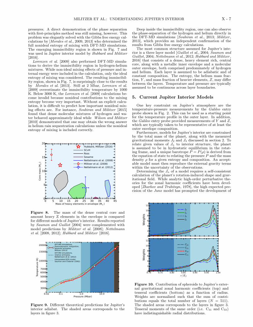
Figure 5. Comparison of the deuterium shock Hugo-niot curves derived with semi-analytical methods (up-per panel: Rogers [1986], Ebeling and Richert [1985a],Saumon and Chabrier [1992], Kerley [1983], Juranek andRedmer [2000], Ross [1998]), shock wave experiments(middle panel: Nellis et al. [1984], Da Silva et al. [1997],Collins et al. [1998], Knudson et al. [2001], Belov et al.[2002], Boriskov [2003]), and first-principles computersimulations (lower panel: [Militzer and Ceperley , 2000],[Lenosky et al., 2000], Bonev et al. [2004]). Changes inbackgound color mark densities equal to 4, 5, and 6 timesthe initial deuterium density of ρ0 = 0.17 g cm−3.

other hand, the different components of the free energy leadto discontinuous first derivatives, a first-order transition, orplasma phase transition (PPT) is inevitably predicted.

The question whether such PPT exists remains contro-versial. Many models have predicted a PPT with a criticalpoint and coexistence region of two fluids characterized bydifferent degrees of ionization and densities. A PPT wasfirst placed on the hydrogen phase diagram by Landau andZeldovich [1943]. First calculations have been made by Nor-man and Starostin [1968] and Ebeling and Sandig [1973].A number of different free energy models such as those by[Saumon and Chabrier , 1992; Kitamura and Ichimaru, 1998;Beule et al., 1999] predict a PPT. The exact location of thecritical point and the coexistence region differ considerablyand other models show continuous transitions [Ross, 1998].Since this was an open question, [Saumon and Chabrier ,1992] provided an alternate model where they smoothly in-terpolate between both regimes.

Path integral Monte Carlo simulations by Magro et al.[1996] showed evidence of a first order transition in dense hy-drogen. However, it was predicted to occur at relatively lowtemperatures [Militzer and Graham, 2006], for which PIMCresults showed some dependence on the choice of fermionnodes. In this temperature regime, density functional molec-ular dynamics (DFT-MD) simulations work very efficiently.A snapshot from such simulations is shown in Fig. 4. Sim-ulations by Vorberger et al. [2007] and Militzer et al. [2008]predicted a gradual molecule-to-metallic transition for tem-perature conditions in the interiors of Jupiter and Saturn.However, at lower temperatures (< 2000K), well below thegiant planet interior adiabats, DFT-MD simulations alsopredict a first-order transition [Morales et al., 2010; Loren-zen et al., 2011].

Significant progress has been made with high pressurelaboratory experiments since the reverberating shock wavemeasurements by Weir et al. [1996] first produced hot,metallic hydrogen in the laboratory. Still it has remaineda challenge to determine whether the molecular-to-metallictransition is of first-order. Measurements by Fortov et al.[2007] and most recently by Knudson et al. [2015] bothshowed evidence of a first-order transition. Still more workis needed to reconcile the results from different experimentswith each other and develop a consistent theoretical frame-work.

The existence of a first-order molecular-to-metallic tran-sition at sufficiently high temperature could introduce a con-vective barrier into Jupiter’s interior. It would thus delaycooling of its interior and stabilize a compositional differencebetween the molecular and metallic layers. Such a differenceis indeed invoked in most models for Jupiter’s interior in or-der to match the gravitational moment J4 but the origin ofthis difference remain poorly understood. We favor the hy-pothesis that the convective barrier was instead introducedby helium rain, which we will discuss in section 4.2. For theinterior models discussed later in this article, we will rely onDFT-MD simulations that predict a gradual molecular-to-metallic transition for pure hydrogen for the temperaturesin Jupiter’s interior.

While unanswered questions remain regarding the phasediagram of dense hydrogen, significant progress has beenmade in characterizing the shock Hugoniot curve of hy-drogen, which is summarized in Fig. 5. Shock wave ex-periments are the preferred laboratory technique [Zeldovichand Raizer , 1968] to determine the equation of state athigh pressure and temperature. During such experiments,a driving force is utilized to propel a pusher at constantvelocity Up into a material at predetermined initial condi-tions (ρ0 = m/V0, P0, T0). The impact generates a planarshock wave, which travels at the constant velocity Us, whereUs > Up. Behind the shock wave, the material reaches

MILITZER ET AL.: UNDERSTANDING JUPITER’S INTERIOR X - 5

a final state thermodynamic equilibrium (ρ = m/V, P, T ).The conservation laws of mass, momentum, and energy, E,across the shock interface leads to the Rankine-Hugoniotequations [Rankine, 1870; Hugoniot , 1887, 1889], which havebeen discussed in detail by Zeldovich and Raizer [1968],

P = 0UsUp + P0 (2)

ρ = ρ0Us

Us − Up(3)

R(ρ, T ) = E − E0 +1

2(V − V0)(P + P0) = 0 . (4)

It is remarkable that the measurements of just Us and Up

allow for an absolute EOS measurement. The shock tem-perature, however, must be determined independently. Theshock Hugoniot curve in Fig. 5 emerges as collection of fi-nal states for different Up. The computation of this curve isstraightforward. For a theoretical EOS provided in term ofE(ρ, T ) and P (ρ, T ), one uses Eq. 4 to solve for R(ρ, T ) = 0by varying ρ at fixed T .

In Fig. 5, we compare the experimental Hugoniotcurves with predictions from analytical techniques and first-principles computer simulations based on PIMC and DFT-MD. Because of shock heating, the temperature along shockHugoniot curve rise significantly more rapidly than that onan adiabat, which makes it difficult to relate shock wavemeasurements to planetary interiors [Militzer and Hubbard ,2007]. In P -ρ space, the Hugoniot curves plot at higherpressures than Jupiter’s adiabat. Nevertheless, these mea-surements provide invaluable constraints for the theoreticalEOS calculations.

In the upper panel of Fig. 5, we compare various analyti-cal EOS models. In the limits of high pressure, all curves areexpected to converge to 4-fold compression, the limiting casefor a non-relativistic gas (ρ/ρ0 = 4). The activity expansion(ACTEX) by Rogers [1986], the Pade approximations in thechemical picture by Ebeling and Richert [1985a] and Saumonand Chabrier [1992] EOS model all predict compression ra-tio of ∼5.5 at 2 Mbar and then converged to limit of 4-foldcompression at higher pressure. The Sesame model by Ker-ley [1983], which has been used frequently to simulate a va-riety of shock processes, predicts a lower shock compressionin comparison. The fluid variational theory (FVT) by Ju-ranek and Redmer [2000] yield compression ratios up to 5.2.The linear mixing model by Ross [1998] stands out amongall EOS models because it predicts shock compression ratiosbetween 5.5 and 6.0 in the entire pressure interval from 1 to4 Mbar.

When laser-driven shock wave experiments by Da Silvaet al. [1997] and Collins et al. [1998] generated megabarpressures in deuterium for the first time, the results weresurprising because they implied shock compression ratios of∼ 6 and therefore favored the linear mixing model by Ross[1998]. These measurements sparked an intense debate inthe high-pressure community and motivated additional ex-perimental and theoretical work. Points of concern werethat neither the PIMC simulations [Militzer and Ceperley ,2000] nor the DFT-MD simulations [Lenosky et al., 2000]could reproduce the results from laser-driven shock mea-surements. Later DFT-MD simulations by Bonev et al.[2004], that treated the molecular phase more accurately,improved the agreement with the gas-gun shock wave ex-periments by Nellis et al. [1984] below 0.25 Mbar but theresults at higher pressure remained unchanged. The agree-ment between the two first-principle simulation methods,PIMC and DFT-MD, is reasonably good, though not yetperfect. This made it possible to put together consistentEOS tables for hydrogen [Militzer and Ceperley , 2001], he-lium [Militzer , 2009], carbon [Benedict et al., 2014], nitro-gen [Driver and Militzer , 2016], oxygen [Driver et al., 2015],water [Driver and Militzer , 2012], neon [Driver and Militzer ,

2015], and most recently silicon [Militzer and Driver , 2015].In each case, results from PIMC simulations that are veryefficient at high temperature were combined with DFT-MDresults at low temperature.

A major contribution towards resolving the controversyregarding the deuterium Hugoniot curve came from magnet-ically driven shock experiments by Knudson et al. [2001],which favor a maximum shock compression ratio of ∼ 4.3,broadly consistent with predictions from first-principles sim-ulations. Later, similar results were reported from spher-ically converging shock wave experiments by Belov et al.[2002] and by Boriskov [2003] as well as by planar shockwave experiments by Brygoo et al. [2015] that were per-formed at the Omega laser facility. Because of all threenew measurements favor a compression of ∼ 4.3, in keepingwith first-principles simulations, one may regard the contro-versy around the deuterium Hugoniot curve to be resolvedwith satisfactory accuracy. If we adopt this view, however,then Saumon et al. [1995] EOS would be no longer the bestEOS to model giant planet interiors because it deviates fromshock measurements for P > 0.7Mbar.

0.2 0.4 0.6 0.8 1.0 1.2 1.4 1.6Density (g cm−3 )

0.5

1.0

1.5

2.0

Pressure (Mbar)

Figure 6. Comparison of the helium shock Hugo-niot curve derived DFT-MD simulations (lines, Militzer[2006, 2009]) and shock wave experiments (symbols, Bry-goo et al. [2015]). The curve represent various initial den-sities in the experiment.

3.2. Experiments and Simulations of Dense Helium

Helium has also been studied with first-principles com-puter simulations and high-pressure experiments, althoughto a lesser extent than hydrogen and deuterium. Early-ondiamond anvil cells (DAC) have been used to explore thesolid phases of helium and its melting curve. Loubeyre et al.[1982] and Vos et al. [1990] measured the melting tempera-ture of helium 4 from 7.4 to 250 kbar and found it to increasefrom 50 to 480 K over this pressure interval. Vos et al. [1990]fit the melting line with a simple power law,

Tmelt = 14.0090 P 0.6390, (5)

with the pressure P in kbar and the melting temperaturein Kelvin. There seems to be some slight deviations fromthis expression at higher pressure [Datchi et al., 2000] butwhen extrapolated to the Mbar pressures, this expression isin good agreement with ab initio estimates of the meltingline [Lorenzen et al., 2009]. Loubeyre et al. [1982] also ob-served a triple point at 299 K and 116.5 kbar between theliquid and possibly an fcc and an hcp solid phase.

X - 6 MILITZER ET AL.: UNDERSTANDING JUPITER’S INTERIOR

The fluid phase of helium has been studied with shockwave experiments [Nellis et al., 1984]. In the experimentsby Eggert et al. [2008], that reached 2 Mbar, diamond cellswere used to increase the initial density of the helium sam-ples. Because of the complexity and the short time scale ofthese experiments, the particle velocity, Up, was not mea-sured directly. Instead of using Eq. 2, the pressures had tobe inferred with an impedance matching construction [Bry-goo et al., 2015] that relied on a reference material withknown properties. For the helium and hydrogen measure-ments, quartz was used as a reference. After the experi-mental results had been published, the quartz shock stan-dard was revised [Knudson and Desjarlais, 2009, 2013] andBrygoo et al. [2015] reinterpreted the existing hydrogen andhelium measurements. The updated helium results are com-pared to predictions from ab initio simulations in Fig. 6.

The EOS of the fluid helium has been characterized byanalytical free energy models by Saumon et al. [1995] andslightly improved by more complete calculations by Winis-doerffer and Chabrier [2005]. More recently, extensive first-principles simulations have been performed using PIMC fortemperatures above 105 K and DFT-MD for the lower tem-peratures [Militzer , 2006, 2009]. The pre-compressed Hugo-niot curves predicted by the ab initio calculations are dis-played in Fig. 6. Overall, there is a good agreement withexperimental results but for small initial densities, the mea-surements predict a slightly higher final shock densities thanthe DFT-MD simulations.

Unlike hydrogen, helium does not exhibit a molecularphase but one still expects it to become a metal at high pres-sure. This phenomenon has been investigated with ab initiosimulations, both by studying the band gap and by comput-ing conductivities and reflectivities. The latter quantity candirectly measured during shock experiments. In the solidphase at 0 K, Khairallah and Militzer [2008] showed bandgap closure occurs at 21.3 g/cm3, or 257 Mbar, using quan-tum Monte Carlo calculation that are in very good agree-ment with predictions from GW density functional theory(GW-DFT). Later calculations with electron-phonon cou-pling by Monserrat et al. [2014] suggested that the metal-lization of helium occurs at even higher pressures. Thus, themetallization pressure of solid helium is at least one order ofmagnitude higher than that of hydrogen, which is expectedto metalize at several Mbar.

The temperature effects on the metallization conditionsof fluid helium were studied by Kowalski et al. [2007] withDFT and GW methods. They showed that the width ofthe gap depends on the temperature and estimated a met-allization density of 10 g/cm3, which was in agreement withcalculations in the chemical picture by Winisdoerffer andChabrier [2005].

The first shock wave experiments that measured the re-flectivity of dense helium ( 1.5 g/cm3) were reported byCelliers et al. [2010]. The size of gap was estimated and gapclosure was predicted to occur at a density of 1.9 g/cm3.A re-analysis of the experimental data by Soubiran et al.[2012], including the temperature effects on the helium gap,showed that experimental findings would also be in agree-ment with a much higher metallization density of 10 g/cm3

or above. This implies that unlike hydrogen, pure heliumwould remain in an atomic and insulating phase over theentire range of pressure-temperature conditions in the inte-rior of giant planets.

4. Hydrogen-Helium Mixtures

4.1. Experiments at Lower Pressure

Because of their significance for planetary science, thehydrogen-helium mixtures have been investigated with var-ious experimental high-pressure techniques. The phase-separation transition in the fluid phase was first studiedwith static anvil cell experiments with an optical observa-tion of the phase transition. Streett [1973] and Schouten

et al. [1985] reported a partial phase separation into twofluids for pressures up to 50 kbar over a temperature inter-val from 26 K to nearly room temperature. Loubeyre et al.[1985, 1987] used the displacement of the hydrogen Q1 modein the Raman spectrum due to the presence of helium to de-termine the mixing phase diagram up to 100 kbar and 373 K.A detailed phase diagram based on the available experimen-tal data is given in Fig. 9 of Loubeyre et al. [1987].

The immiscibility of hydrogen and helium depends ontemperature, pressure, and the concentration. For low he-lium concentration, the demixing is mostly related to thecrystallization of hydrogen. For a slightly higher heliumconcentrations, a triple point is observed for temperaturesbetween 100 and 373 K as the helium concentration is in-creased from 0.11 to 0.32. This triple point is an equilibriumbetween a hydrogen-rich solid phase and two liquid phasesof intermediate and high helium concentrations.

Loubeyre et al. [1987] also defined a critical point that,for a given temperature, marks the minimum pressure forany mixtures to show phase separation. For instance, at295 K, the critical point is at 51 kbar, while the triple pointis at 62 kbar (see Fig. 9 of Loubeyre et al. [1987]). Whilethese results represent the best laboratory measurements ofhydrogen-helium mixtures to date, their relevance for the ex-treme pressure and temperature conditions in giant planetinteriors remains to be determined.

4.2. Simulations of Hydrogen-Helium Phase Separation

Because of the relevance to giant planet interiors,hydrogen-helium mixtures have been the subject of variousfirst-principles studies. Early DFT simulations by Klepeiset al. [1991] and Pfaffenzeller et al. [1995] focused on groundstate calculations of solid hydrogen-helium mixtures becauseDFT-MD simulation at high temperature could not yet beenperformed efficiently. Homogeneous hydrogen-helium mix-tures were also studied with path integral Monte Carlo sim-ulations [Militzer , 2005] but it has proved challenging toapply this method below 10 000K where one expects phaseseparation in the fluid.

Once more computer time became available, Vorbergeret al. [2007] studied nonlinear mixing effects in hydrogen-helium mixtures with DFT-MD simulations. It was demon-strated that, for a given pressure and temperature, the pres-ence of helium stabilizes the hydrogen molecules and shiftsthe molecular-to-metallic transition in hydrogen to higher

0.2 0.5 1 2 5 10 20 50Pressure (Mbar)

0

1

2

3

4

5

6

7

8

9

10

11

12

Temperature (1000 K)

Pressure at Saturn's

core-m

antle boundary

Pressure at Jupiter's

core-m

antle boundary

H-He immiscibility regionMorales et al. (2013)

Immiscibility regionLorenzen (2009)

Young, fully mixed

giant planet (S=7.40)

Helium rain ..... starts (S=7.20)

Jupiter's en

tropy (S=7

.08)

Satur

n's en

tropy (S=6

.84)

Figure 7. Hydrogen-helium miscibility diagram. Thesolid lines show DFT-MD adiabats from Militzer andHubbard [2013] labeled with their entropy in units of kbper electron. The shaded area is the immiscibility regioncalculated by Morales et al. [2013] that we extrapolatedtowards higher pressures.

MILITZER ET AL.: UNDERSTANDING JUPITER’S INTERIOR X - 7

pressures. A direct demonstration of the phase separationwith first-principles method was still missing, however. Thisproblem was elegantly solved with the Gibbs free energy cal-culations by [Morales et al., 2009, 2013] who determined thefull nonideal entropy of mixing with DFT-MD simulations.The emerging immiscibility region is shown in Fig. 7 andwas used in Jupiter interior model by Hubbard and Militzer[2016].

Lorenzen et al. [2009] also performed DFT-MD simula-tions to derive the immiscibility region in hydrogen-heliummixtures. While non-ideal mixing effects of pressure and in-ternal energy were included in the calculation, only the idealentropy of mixing was considered. The resulting immiscibil-ity region, shown in Fig. 7, is surprisingly close to the resultsby Morales et al. [2013]. Still at 2 Mbar, Lorenzen et al.[2009] overestimate the immiscibility temperature by 1000K. Below 3000 K, the Lorenzen et al. [2009] calculations be-come invalid because nonideal contributions to the mixingentropy become very important. Without an explicit calcu-lation, it is difficult to predict how important nonideal mix-ing effects are. For instance, Soubiran and Militzer [2015]found that dense molecular mixtures of hydrogen and wa-ter behaved approximately ideal while Wilson and Militzer[2010] demonstrated that one may obtain the wrong answerin helium rain sequestration calculations unless the nonidealentropy of mixing is included correctly.

0 5 10 15 20 25 30 35 40 45Mass of heavy elements in envelope (ME )

0

5

10

15

20

Core m

ass

(ME)

Hubbard, Militzer (2016)

SCvH

Ross

Sesame

Nettelmann et al. (2008)

Militzer et al. (2008)

Nettelmann et al. (2012)

Figure 8. The mass of the dense central core andamount heavy Z elements in the envelope is comparedfor different models of Jupiter’s interior. Results reportedby Saumon and Guillot [2004] were complemented withmodel predictions by Militzer et al. [2008]; Nettelmannet al. [2008, 2012]; Hubbard and Militzer [2016].

0.02 0.1 1.0 10.0Pressure (Mbar)

3000

4000

5000

6000

7000

10000

15000

20000

Temperature (K)

DFT-MD simulations,thermodynamic integration,absolute entropies,Militzer (2013)

DFT-MD simulations,relative entropies,Nettelmann et al. (2012)

Interpolated EOS model,Saumon and Chabrier (1992)

Figure 9. Different theoretical predictions for Jupiter’sinterior adiabat. The shaded areas corresponds to thelayers in figure 3.

Deep inside the immiscibility region, one can also observethe phase-separation of the hydrogen and helium directly inthe DFT-MD simulations [Soubiran et al., 2013; Militzer ,2013], which provides an independent confirmation of theresults from Gibbs free energy calculations.

The most common structure assumed for Jupiter’s inte-rior is a three layer model [Guillot et al., 2004; Saumon andGuillot , 2004; Nettelmann et al., 2012; Hubbard and Militzer ,2016] that consists of a dense, heavy element rich, centralcore, along with a metallic inner envelope and a molecularouter envelope, both comprised predominately of hydrogenand helium. Each layer is assumed to be adiabatic and ofconstant composition. The entropy, the helium mass frac-tion, Y , and mass fraction of heavier elements, Z, may differbetween the layers. Temperature and pressure are typicallyassumed to be continuous across layer boundaries.

5. Current Jupiter Interior Models

One key constraint on Jupiter’s atmosphere are thetemperature-pressure measurements by the Galileo entryprobe shown in Fig. 2. This can be used as a starting pointfor the temperature profile in the outer layer. In addition,the Galileo entry probe provided measurements of Y and Z,which are typically taken to be representative of at least theouter envelope composition.

Furthermore, models for Jupiter’s interior are constrainedby the total mass of the planet, along with the measuredgravitational moments J2 and J4 discussed in section 2. Torelate given values of Jn to interior structure, the planetis assumed to be in hydrostatic equilibrium in the rotat-ing frame, and a unique barotrope P = P (ρ) is derived fromthe equation of state to relating the pressure P and the massdensity ρ for a given entropy and composition. An accept-able model must then reproduce the external gravity termswithin the uncertainty of the observations.

Determining the Jn of a model requires a self-consistentcalculation of the planet’s rotation-induced shape and grav-itational field. While analytic high-order perturbative the-ories for the zonal harmonic coefficients have been devel-oped [Zharkov and Trubitsyn, 1978], the high expected pre-cision of the Juno model has prompted the development of

0

2

4

6

8

10

12

Weights

J2J4J6J8

0.70 0.75 0.80 0.85 0.90 0.95 1.00

r/RJ

0

2

4

6

8

10

12

Weights

C22

C31

C42

C51

Figure 10. Contribution of spheroids to Jupiter’s exter-nal gravitational zonal harmonic coefficients (top) andtesseral coefficients (bottom) as a function of radius.Weights are normalized such that the sum of contri-butions equals the total number of layers (N = 511).The shaded areas corresponds to the layers in figure 3.Tesseral moments of the same order (i.e. C31 and C33)have indistinguishable radial distributions.

X - 8 MILITZER ET AL.: UNDERSTANDING JUPITER’S INTERIOR

more precise non-perturbative, numerical methods for cal-culating Jn [Hubbard , 2013; Wisdom and Hubbard , 2016].Using this method, Hubbard and Militzer [2016] suggestedthat the actual J4 of Jupiter might lie outside of the errorbars reported by Jacobson [2003] in order to be consistentwith the DFT-MD equation of state byMilitzer and Hubbard[2013].

In Fig. 8, we compare the core sizes and amounts ofheavy Z elements in the outer layers that were inferred frommodel calculations that assumed various EOSs of hydrogen-helium mixtures. The large spread of predictions by dif-ferent equations of state highlights the importance of anaccurate equation of state for the interpretation of measure-ments by Juno and future missions. Interior models basedon the Sesame [Kerley , 1983], Ross [1998], and Saumonet al. [1995] EOSs yield core masses of less than 10 M⊕ andwould thus be inconsistent with the core accretion assump-tion for the planet’s formation [Pollack et al., 1996] unlessan initial dense core has been eroded by convection (seesection 6.3). However, these EOSs all yield substantial coremasses between 10 and 25 M⊕ for Saturn’s interior [Saumonand Guillot , 2004]. This means, if core erosion indeed oc-curred in giant planet interiors, it had to be much stronger inJupiter’s interior than in Saturn. This is not inconceivablesince Jupiter is three time heavier and thus more convectiveenergy would be available to lift up heavy materials againstforces of gravity.

On the other hand, Jupiter interior models on DFT-MDEOS by Militzer et al. [2008] and Hubbard and Militzer[2016] predict a larger central core for Jupiter of 12 M⊕

or more. The latter model assumed that helium rain oc-curred on this planet, which suggests Jupiter’s interior maynot be too different from that of Saturn. The DFT-MDbased models by Nettelmann et al. [2008, 2012] predict avery small central core of 8 M⊕ or less, which requires fur-ther discussion.

Figure 9 shows that the adiabats are very different. Mil-itzer and Hubbard [2013] computed absolute entropies. Eachpoint in Fig. 9 was determined with an independent calcu-lation with the ab initio thermodynamic integration (TDI)method [de Wijs et al., 1998; Alfe et al., 2000; Morales et al.,2009; Wilson and Militzer , 2010]. The fact that a smoothcurve emerges demonstrates that the statistical error barscan be controlled very well with TDI approach [Militzer ,2013]. The computed ab initio entropies also agree well withthe Saumon et al. [1995] EOS model in the limit of low andhigh pressure where one expects this semi-analytical modelto work well since it was designed to reproduce the EOS ofa weakly interacting molecular gas at low pressures and atwo-component plasma in the high-pressure limit. For inter-mediate pressures from 0.2 to 20 Mbar, figure 9 shows devi-ations between the ab initio TDI approach [Militzer , 2013]and Saumon et al. [1995] EOS model because little informa-tion about the properties of hydrogen near the molecular-to-metallic transition was available when this model was con-structed. Furthermore, the deviations are seen in a regionwhere Saumon et al. [1995] interpolated between their de-scriptions for molecular and metallic hydrogen. Deviationsin this regions are, thus, not unexpected.

It is unusual, however, that the adiabats DFT-MD byNettelmann et al. [2012] are significantly higher in temper-ature than those by Militzer and Hubbard [2013].

There are three main reasons for the deviations in the abinitio adiabats in Fig. 8 that need to be considered. (1)Since Nettelmann et al. [2012] did not use the TDI tech-nique, absolute entropies could not be determined. Insteadthe slope of the adiabat was inferred from the pressure andinternal energies that are accessible with standard ab initiosimulations. In addition to the slope, an anchor point at∼0.1 Mbar is needed to start the computation of the adi-abat. Already at this low pressure, the Nettelmann et al.[2012] abiabat is significantly higher than that reported byMilitzer and Hubbard [2013]. If the anchor point in the Net-telmann et al. [2012] calculation is chosen differently, the

agreement of the adiabats improves substantially (see Fig.11 in Militzer and Hubbard [2013]).

(2) When the slopes of the adiabats are determined fromthe ab initio pressures and internal energy, (∂T/∂V )S =−T (∂P/∂T )V / (∂E/∂T )V [Militzer , 2009], one needs Pand E on a fine grid of density-temperature points for inter-polation. In practice, one can only perform a finite numberof simulations and the results have statistical uncertainties.

(3) Finally, Nettelmann et al. [2012] computed the EOSfor hydrogen and helium separately and then invoked lin-ear mixing approximation to characterize the H-He mixturewhile Militzer and Hubbard [2013] performed fully interact-ing simulations on one representative H-He mixture withmixing ratio (Y=0.245) and then used the linear mixingapproximation only to perturb around this concentration.However, far outside of the H-He immiscibility region oneexpects the linear mixing approximation to be reasonable.

We gathered that the last two points are of lesser impor-tance and concluded that the main reason for the deviationsin Fig. 8 was the choice to take an anchor point from theanalytical fluid variational theory [Nettelmann et al., 2012].

The temperature profile is important for models of gi-ant planet interiors. For a given pressure, a higher temper-ature implies a lower density, which is compensated by ahigher fraction of heavy Z elements when Jupiter interiormodels are constructed with the goal of matching the mea-sured values of the planet’s gravity field. A higher-than-solarheavy element fraction would imply that the process, thatled to Jupiter’s formation, was more efficient in capturingdust and ice than gas. Therefore the characterization of H-He adiabats with theoretical and experimental techniques isimportant to understand Jupiter’s formation. At the sametime, the interaction of heavy Z elements with dense H-Hemixtures needs to be characterized. Soubiran and Militzer[2016] performed simulations for a variety of heavy elements.This is the first study to investigate the properties of multi-component mixtures of H, He and heavy elements. It showsthat the heavy elements slightly influence the density profileof giant planets. Fig. 4 shows one representative snapshotfrom a ternary hydrogen-helium-iron mixture.

Giant planet interior models often invoke a differentchemical composition for molecular and metallic layers. Theoriginal justification for introducing this additional degree offreedom was a first order phase transition between molecu-lar and metallic hydrogen. This argument is not supportedby DFT-MD simulations that show a smooth transition ofproperties with increasing P Vorberger et al. [2007]; Militzeret al. [2008]. More recently it has been proposed that theseparation between layers in Jupiter corresponds to a narrowregion of helium immiscibility [Guillot et al., 2004; Hubbardand Militzer , 2016]. A schematic depiction of this model isshown in Figure 3. The precipitation of helium through thislayer is expected to lead to an intrinsic density differencethat may inhibit effective convection between the inner andouter envelope. This may allow Jupiter’s deep interior to behotter than would be expected for a single layer convectionenvelope. Hubbard and Militzer [2016] identify this region byidentifying the pressures where the present-day adiabat forthe outer envelope intersects H-He immiscibility region fromMorales et al. [2013] (Figure 2). This leads to a predictionof a present-day helium rain region between ∼ 0.81− 0.88a.This model has an important evolutionary distinction, sincethe planet’s temperature profile would have initially beenabove the immiscibility region, meaning the envelope is ini-tially homogeneous, with the demixing layer forming andgrowing as the planet cools.

Figure 10 shows the contribution functions for zonal andtesseral harmonics of degree 2, 4, 6, and 8. As suggested byEq. 1, these functions are progressively more peaked towardthe surface with increasing degree. There is no significant

MILITZER ET AL.: UNDERSTANDING JUPITER’S INTERIOR X - 9

direct contribution from the central region where a centralcore might exist. Moreover, the contribution functions over-lap substantially, implying that values of the harmonics for agiven density distribution are strongly correlated. The massof a dense central core cannot be inferred solely from a finiteset of harmonic coefficients; instead it must emerge from asimultaneous fit to all available constraints on interior struc-ture. This process is strongly dependent on the precision ofthe thermodynamic model used to construct the barotrope.

6. Discussion of Jupiter Models

6.1. The Adiabatic Assumption

The modeling of a giant planet’s thermal structure rely ona few simple equations once spherical symmetry is assumed.The first arises from the conservation of mass,

dm

dr= 4πr2ρ, (6)

where m is the mass enclosed in a sphere of radius r andρ the local density. Second, one assumes hydrostatic equi-librium, which is a reasonable assumption as no shocks orother dynamical effects of any significance are present. Thisprovides a constraint on the pressure profile:

dP

dr= −

Gmρ

r2, (7)

where P is the local pressure and G is the gravitational con-stant. In the simplest case, just one additional relationshipis required to determine the interior structure of a planet,which is the equation of state, ρ = ρ(P, T ), of the materialin each layer. This require one to introduce additional as-sumptions for the temperature profile unless the pressure isdominated by contributions from a degenerate electron gas.In general the temperature profile, T (r), is set by the pro-cesses that transfer thermal energy throughout the planet.The relationship of the temperature and pressure profilescan be expressed in the following convenient form,

dT

dr=

T

P

dP

dr∇(T, P ) , (8)

with the temperature gradient ∇(T, P ) ≡ d lnT

d lnP, which is

set by the energy transfer mechanisms. In the interiors of

2 5 10 20 50Pressure (Mbar)

10-1

100

101

102

Gradient

∇cond

∇ad

Figure 11. Adiabatic and conductive gradients along aJupiter-type profile. The model and the adiabatic gra-dient are computed with the SCvH EOS [Saumon et al.,1995]. The thermal conductivity is estimated with thefully ionized model [Potekhin et al., 2015]. The shadedareas corresponds to the layers in figure 3.

planets and stars, there are three possible mechanisms ofenergy transfer: radiation, convection, and conduction. Tofirst approximation, the process that leads to smallest tem-perature gradient will be the most efficient one and thereforedominate the energy transfer in a particular layer.

∇(T, P ) = min(∇ad,∇rad,∇cond). (9)

The adiabatic gradient, ∇ad, corresponds to the temper-ature gradient that arises in a convecting material. It is de-termined by making the assumption that an advected parcelof fluid rises fast enough to prevent energy loss through dif-fusion or radiation to the surrounding fluid. We also assumethat the evolution is slow enough for the pressure inside andoutside of the parcel to reach an equilibrium. In this case thetransformation is quasi-static and thus isentropic. The re-sulting adiabatic gradient directly follows from the equationof state,

∇ad =∂ lnT

∂ lnP

∣

∣

∣

S. (10)

In the case of a purely conductive layer, the thermal conduc-tivity, λ, is the key quantity. From Fourier’s law, we knowthat the heat flux through the sphere of radius r is given by

F (r) = −λdT

dr. The heat flux is related to the luminosity, l,

by F (r) = l(r)

4πr2. From these relations and Eq. 7, we find,

∇cond =lP

4πλTGmρ. (11)

In case of a purely radiative layer, under the diffusive ap-proximation, we find that the radiative gradient is given by[Rutten, 2003]:

∇rad =3κlP

64πσT 4Gm, (12)

with κ the opacity of the material and σ the Stefan-Boltzmann constant.

We can perform an order-of-magnitude calculation to de-termine which energy transfer mechanism dominates in dif-ferent layers of a giant planet. Radiation is only importantin the upper most atmosphere because the radiative opac-ity is high in all deeper layers. For instance in the metallicregion in the deep interiors of giant planets, free electronsabsorb photons very efficiently. In Fig. 11, we compare theconductive and adiabatic gradients for the interior of a giantplanet. The adiabatic gradient was derived from the equa-tion of state by Saumon et al. [1995]. For this comparison,one can assume that the luminosity is constant throughoutthe envelope [Mordasini et al., 2012] and use the value of8.7× 10−10L⊙.

An approximate value for thermal conductivity can be de-rived from the fully ionized model of Potekhin et al. [2015],which an upper limit for the conductivity because not allelectrons are fully ionized and scattering processes matterin dense hydrogen-helium mixtures. Fig. 11 underlines thatthe adiabatic gradient is nearly two orders of magnitudelower than the conductive gradient which indicates that theconvection is the most efficient mechanism and that the isen-tropic approximation is valid as long as the envelope has ahomogeneous composition.

6.2. Over-turning and Double-Diffusive Convection

The adiabatic assumption relies on the hypothesis thatthe envelope is entirely and efficiently convective. However,as Stevenson [Stevenson, 1985] pointed out more than threedecades ago, the interior of a giant planet may not be ho-mogeneous in composition for a number of reasons including

X - 10 MILITZER ET AL.: UNDERSTANDING JUPITER’S INTERIOR

late planetesimal accretion, core erosion and phase separa-tion. In this case, even if the thermal density gradient isdestabilizing, an intrinsic density gradient of compositioncan become stabilizing if there is an excess of heavy mate-rials in the warm regions and lighter materials in the coldregions. This process is termed double-diffusive convectionor semi-convection in the literature. To characterize the be-havior of the fluid in the presence of a gradient of tempera-

ture ∇T = d lnT

d lnPand a gradient of mean molecular weight

(equivalent to a gradient of composition) ∇µ = d lnµ

d lnP, we

define a density ratio [Stern, 1960; Leconte and Chabrier ,2012]:

Rρ =αT

αµ

∇T −∇ad∇µ

, (13)

with αT = −∂ ln ρ∂ lnT

∣

∣

P,µand αµ = ∂ ln ρ

∂ lnµ

∣

∣

P,T. In the case of

a destabilizing temperature gradient, ∇T − ∇ad > 0, buta stabilizing compositional gradient, ∇µ > 0, the convec-tive instability criterion then becomes R−1

ρ < 1, called theLedoux criterion [Ledoux , 1947]. However, this is not a sim-ple stability criterion and there are three different observedbehaviors (see Fig. 1 in Leconte and Chabrier [2012] for aschematic diagram).

The stability criterion is given by

R−1ρ >

Pr + 1

Pr + τ, (14)

with Pr = νκT

, the Prandtl number, which is the ratio be-tween the kinematic viscosity and the thermal diffusivity,and τ = D

κT

, the ratio of the solute particle diffusivity andthe thermal diffusivity. If this criterion is verified then thelayer is stably stratified and no dynamics is expected.

In the case of a marginally stable system,

R−1

min < R−1ρ ≤

Pr + 1

Pr + τ, (15)

a system of oscillatory convection, also called turbulent dif-fusion, can occur.

The last case is the layered convection where well-definedlayers develop with a small-scale convection, when

1 < R−1ρ ≤ R−1

min. (16)

The critical value of R−1

mindepends on the properties of the

fluid under study and its exact value is difficult to estimate[Radko, 2003; Rosenblum et al., 2011; Mirouh et al., 2012].

While the oscillatory convection seems irreconcilable withthe observed heat flux of Jupiter or Saturn [Leconte andChabrier , 2013; Nettelmann et al., 2015], layered convec-tion could explain the observed properties of the planets. Inthis layered convection, the envelope is divided in successivelayers alternating between convective sub-cells and diffusivelayers of height hc and hd respectively. In a steady state, thetypical timescale for the diffusive and the convective layershave to be similar leading to a height ratio:

hdhc

= Ra−1/4⋆ , (17)

where Ra⋆ is the modified Rayleigh number defined as[Leconte and Chabrier , 2012; Spruit , 2013]:

Ra⋆ =αT gH

3P

κ2T

α4(

∇T −∇ad)

, (18)

with g the local gravitational acceleration, HP the pressurescale height and α = hc/HP . It is interesting to note in

Eq. (17), that the heights ratio is proportional to κ1/2T .

Yet, there is a significant difference when one uses the fullyionized model [Potekhin et al., 2015] or the ab initio calcu-lations [French et al., 2012] to estimate the thermal diffu-sivity, leading to significant uncertainty in the height ratio.Secondly, Eq. (18) shows that α is a key parameter yetunconstrained a priori.

Leconte and Chabrier [2012] explored the possible giantplanet structures when layered convection is assumed. If weconsider a fixed α throughout the envelope, it is possibleto build models that match all the observable properties ofJupiter and Saturn, including the heat flux and the gravi-tational moments. The permitted values for α for Jupiterrange from 3× 10−5 to 10−2 which gives a number of layersranging between 100 and 3 × 104. For a higher number oflayers, the interior becomes too hot and the average densitytoo low. A very interesting outcome of the layered convec-tion assumption is that the total content of heavy elementincreases from 40 M⊕ in the adiabatic case to 63 M⊕ for themost extreme layered convection considered, out of whichonly 0-0.5 M⊕ is in a dense central core. Moreover, as thelayered convection is less efficient than large-scale convec-tion in transporting heat, they suggested it as a possibleexplanation of the excess luminosity of Saturn [Leconte andChabrier , 2013].

Leconte and Chabrier [2012] did not make any assump-tion on the origin of the initial gradient of composition fortheir layered convection model, but one possible origin isthe phase separation of hydrogen and helium [Christensenand Yuen, 1985]. When considering a layered or double-diffusive convection, the fluxes of heat and of compositionmust be carefully characterized since they affect the evolu-tion of the planet’s interior. To better constrain the evolu-tion of Jupiter in the case of a H-He phase separation, Net-telmann et al. [2015] used numerical results of layered anddouble-diffusive convection simulations with scaling laws forthe heat flux [Mirouh et al., 2012; Wood et al., 2013]. How-ever, these scaling laws were computed for the case of mis-cible fluids and do not consider the possible influence thephase separation may have on the fluxes. Nettelmann et al.[2015] based their model on thermodynamic properties com-ing from the SCvH EOS [Saumon et al., 1995] and on thephase diagram computations of Lorenzen et al. [2009, 2011].They observed that to match the Galileo probe measuredhelium abundance they needed to modify the shape of thephase diagram, or the outer layer would become too depletedin helium. They also found that Jupiter’s cooling age wastoo long by 1.1 Gyr with He rain and the adiabatic assump-tion (their Figure 16). In the case of a layered convection,they found possible models that would match the observa-tions and the age of Jupiter with layers of 100 to 1000 mheight.

While important advances have been made using non-adiabatic models, they have also raised many questions thatneed to be addressed to understand the formation of lay-ered convection state. First, the H-He phase diagram mustbe better constrained. Likewise, the heat and particle fluxesmust be better constrained along with the influence of thephase separation and corresponding release of latent heat.Last, the length scale of the convective cells is likely to evolvein time with merging mechanisms [Spruit , 2013] that will becompeting with the phase separation. The dynamical ef-fects of these different phenomena could have an importantimpact on the predicted evolution of the giant planets.

6.3. Core Erosion

The existence and size of a dense central core of Jupiter isan outstanding question. Although a dense central core is anatural outcome of the preferred core accretion hypothesis

MILITZER ET AL.: UNDERSTANDING JUPITER’S INTERIOR X - 11

for Jupiter’s formation [Mizuno et al., 1978; Bodenheimerand Pollack , 1986; Pollack et al., 1996], it would not nec-essarily result in a planet formed by the collapse region ofthe disk under self-gravity, e.g. [Boss, 1997]. Moreover, ithas been suggested by Stevenson [1982], that at high pres-sures the stable phases of the high-density materials maybecome soluble in liquid hydrogen. As a result, an initialdense core with rocky or icy composition might erode, withthe dense material being redistributed over a larger regionof the planet. This is one mean of forming a density gra-dient necessary for a double diffusive region in the planet’sinterior [Chabrier and Baraffe, 2007; Leconte and Chabrier ,2012; Mirouh et al., 2012]. While many interior models (e.g.[Hubbard and Militzer , 2016]) require a dense central coreof up to ∼20 Earth masses to match the observed gravi-tational moments, the model predictions are not sensitiveto the radius, or equivalently density, of this core. Variouscore compositions are plausible. It could be a terrestrialiron-rock mixture, a iron-rock-ice mixture, or be a more dif-fuse mixture of heavy elements with liquid hydrogen andhelium.

The solubility of various materials have been assessedwith DFT-MD calculations comparing Gibbs free energy ofthe solution compared to the separated materials. This isaccomplished by performing DFT-MD simulations with atwo-step thermodynamic integration method [Morales et al.,2009; Wilson and Militzer , 2010]. A number of studies usedthis to find the solubility of various analogue planetary ma-terials in liquid metallic hydrogen. Dissolution was found tobe strongly favorable for both water [Wilson and Militzer ,2012a] and iron [Wahl et al., 2013] in the cores of Jupiterand Saturn. Solubility of rocky analogues MgO [Wilson andMilitzer , 2012b] and SiO2 [Gonzalez-Cataldo et al., 2014] aremore moderate, but are still predicted to dissolve in Jupiter’sinterior. The high-pressure solubility of all these materialswith metallic hydrogen is consistent with their increasingmetallic nature at high pressures. Thus a dense central coreof Jupiter is expected to be presently eroded or eroding.However, the redistribution of heavy elements by inefficientdouble-diffusive convection may be slow compared to evo-lutionary timescales [Chabrier and Baraffe, 2007], keepingmost of the heavy elements confined to a relatively smallregion in the planet’s deep interior.

7. Conclusions

Despite the obvious difficulties to predict how the fieldsof planetary science and high-pressure physics will developin the coming 25 years, a few statements can be made. AfterJuno, we expect further space missions to visit all four gi-ant planets in our solar system. Since Uranus and Neptunehave not been studied as often as Jupiter and Saturn, we ex-pect to gather fundamental knowledge about the history ofouter solar system from future ice giant missions. It wouldbe worthwhile to include entry probes since they provideso much more detailed information about the atmosphericcomposition than remote observations can.

We also expect first-principles computer simulations tobecome more accurate. Standard DFT-MD methods maybe replaced with quantum Monte Carlo methods.

As far as high-pressure laboratory experiments are con-cerned, a direct measurements of hydrogen-helium phaseseparation would be of significant importance for our un-derstanding of gas giant interiors. We also anticipate thatcold, metallic hydrogen will be produced in static compres-sion experiments at room temperature.

Acknowledgments

The authors knowledge support from the U.S. NationalScience Foundation, from the NASA mission Juno and aCassini data analysis grant. T. Guillot provided valuable

comments on Fig. 2. The data in the figures can be ob-tained from the references or by contacting the first author.

References

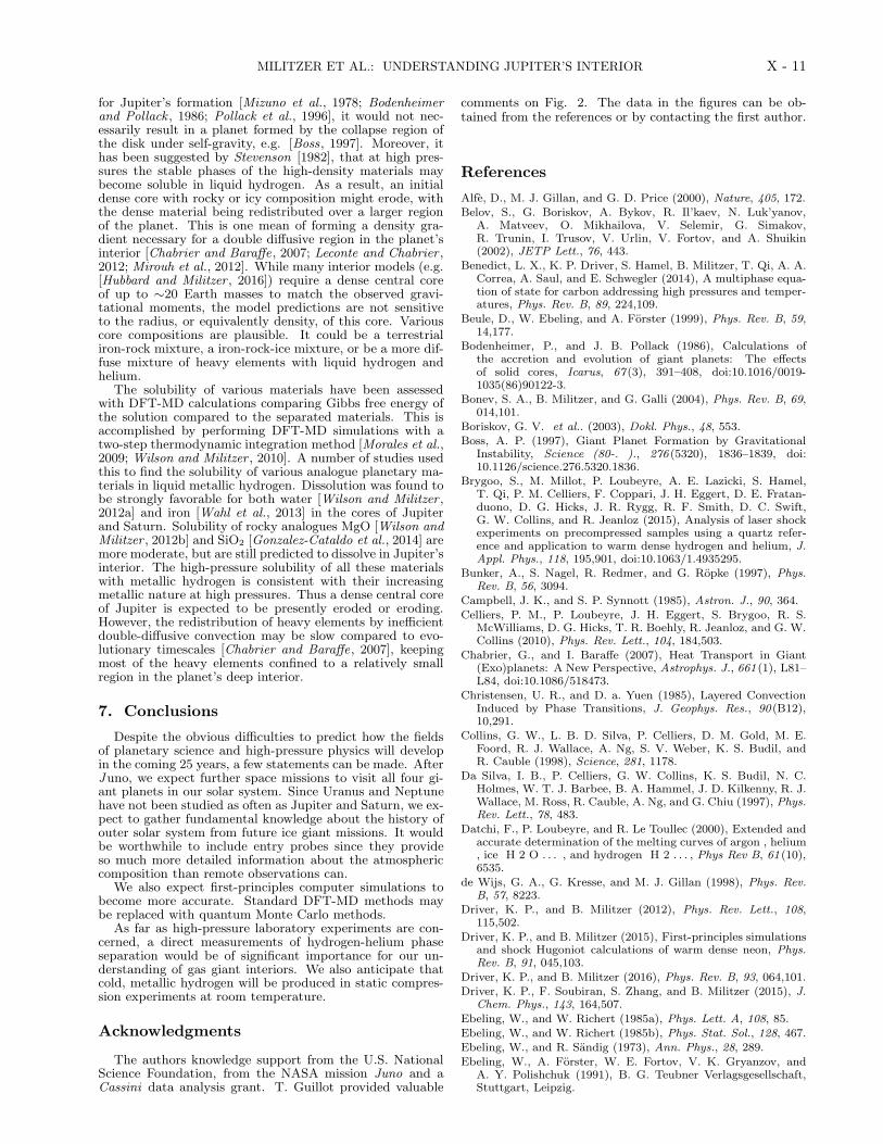
Alfe, D., M. J. Gillan, and G. D. Price (2000), Nature, 405, 172.Belov, S., G. Boriskov, A. Bykov, R. Il’kaev, N. Luk’yanov,

A. Matveev, O. Mikhailova, V. Selemir, G. Simakov,R. Trunin, I. Trusov, V. Urlin, V. Fortov, and A. Shuikin(2002), JETP Lett., 76, 443.

Benedict, L. X., K. P. Driver, S. Hamel, B. Militzer, T. Qi, A. A.Correa, A. Saul, and E. Schwegler (2014), A multiphase equa-tion of state for carbon addressing high pressures and temper-atures, Phys. Rev. B, 89, 224,109.

Beule, D., W. Ebeling, and A. Forster (1999), Phys. Rev. B, 59,14,177.

Bodenheimer, P., and J. B. Pollack (1986), Calculations ofthe accretion and evolution of giant planets: The effectsof solid cores, Icarus, 67 (3), 391–408, doi:10.1016/0019-1035(86)90122-3.

Bonev, S. A., B. Militzer, and G. Galli (2004), Phys. Rev. B, 69,014,101.

Boriskov, G. V. et al.. (2003), Dokl. Phys., 48, 553.Boss, A. P. (1997), Giant Planet Formation by Gravitational

Instability, Science (80-. )., 276 (5320), 1836–1839, doi:10.1126/science.276.5320.1836.

Brygoo, S., M. Millot, P. Loubeyre, A. E. Lazicki, S. Hamel,T. Qi, P. M. Celliers, F. Coppari, J. H. Eggert, D. E. Fratan-duono, D. G. Hicks, J. R. Rygg, R. F. Smith, D. C. Swift,G. W. Collins, and R. Jeanloz (2015), Analysis of laser shockexperiments on precompressed samples using a quartz refer-ence and application to warm dense hydrogen and helium, J.Appl. Phys., 118, 195,901, doi:10.1063/1.4935295.

Bunker, A., S. Nagel, R. Redmer, and G. Ropke (1997), Phys.Rev. B, 56, 3094.

Campbell, J. K., and S. P. Synnott (1985), Astron. J., 90, 364.Celliers, P. M., P. Loubeyre, J. H. Eggert, S. Brygoo, R. S.

McWilliams, D. G. Hicks, T. R. Boehly, R. Jeanloz, and G. W.Collins (2010), Phys. Rev. Lett., 104, 184,503.

Chabrier, G., and I. Baraffe (2007), Heat Transport in Giant(Exo)planets: A New Perspective, Astrophys. J., 661 (1), L81–L84, doi:10.1086/518473.

Christensen, U. R., and D. a. Yuen (1985), Layered ConvectionInduced by Phase Transitions, J. Geophys. Res., 90 (B12),10,291.

Collins, G. W., L. B. D. Silva, P. Celliers, D. M. Gold, M. E.Foord, R. J. Wallace, A. Ng, S. V. Weber, K. S. Budil, andR. Cauble (1998), Science, 281, 1178.

Da Silva, I. B., P. Celliers, G. W. Collins, K. S. Budil, N. C.Holmes, W. T. J. Barbee, B. A. Hammel, J. D. Kilkenny, R. J.Wallace, M. Ross, R. Cauble, A. Ng, and G. Chiu (1997), Phys.Rev. Lett., 78, 483.

Datchi, F., P. Loubeyre, and R. Le Toullec (2000), Extended andaccurate determination of the melting curves of argon , helium, ice H 2 O . . . , and hydrogen H 2 . . . , Phys Rev B, 61 (10),6535.

de Wijs, G. A., G. Kresse, and M. J. Gillan (1998), Phys. Rev.B, 57, 8223.

Driver, K. P., and B. Militzer (2012), Phys. Rev. Lett., 108,115,502.

Driver, K. P., and B. Militzer (2015), First-principles simulationsand shock Hugoniot calculations of warm dense neon, Phys.Rev. B, 91, 045,103.

Driver, K. P., and B. Militzer (2016), Phys. Rev. B, 93, 064,101.Driver, K. P., F. Soubiran, S. Zhang, and B. Militzer (2015), J.

Chem. Phys., 143, 164,507.Ebeling, W., and W. Richert (1985a), Phys. Lett. A, 108, 85.Ebeling, W., and W. Richert (1985b), Phys. Stat. Sol., 128, 467.Ebeling, W., and R. Sandig (1973), Ann. Phys., 28, 289.Ebeling, W., A. Forster, W. E. Fortov, V. K. Gryanzov, and

A. Y. Polishchuk (1991), B. G. Teubner Verlagsgesellschaft,Stuttgart, Leipzig.

X - 12 MILITZER ET AL.: UNDERSTANDING JUPITER’S INTERIOR

Eggert, J., S. Brygoo, P. Loubeyre, R. S. McWilliams, P. M.Celliers, D. G. Hicks, T. R. Boehly, R. Jeanloz, and G. W.Collins (2008), Hugoniot data for helium in the ioniza-tion regime, Phys. Rev. Lett., 100 (March), 124,503, doi:10.1103/PhysRevLett.100.124503.

Fortov, V. E., R. I. Ilkaev, V. A. Arinin, V. V. Burtzev, V. A.Golubev, I. L. Iosilevskiy, V. V. Khrustalev, A. L. Mikhailov,M. A. Mochalov, V. Y. Ternovoi, and M. V. Zhernokletov(2007), Phys. Rev. Lett., 99, 185,001.

Fowler, R., and E. Guggenheim (1965), Cambridge UniversityPress, Cambrdige, UK.

French, M., A. Becker, W. Lorenzen, N. Nettelmann, M. Bethken-hagen, J. Wicht, and R. Redmer (2012), Ab Initio Simulationsfor Material Properties Along the Jupiter Adiabat, Astrophys.J. Suppl. Ser., 202 (2011), 5, doi:10.1088/0067-0049/202/1/5.

Galileo (), Galileo probe archive, http://pds-atmospheres.nmsu.edu/cgi-bin/getdir.pl?volume=gp 0001,accessed: 2016-07-21.

Gonzalez-Cataldo, F., H. F. Wilson, and B. Militzer (2014), As-trophys. J., 787, 79.

Guillot, T., D. J. Stevenson, W. B. Hubbard, and D. Saumon(2004), The interior of Jupiter, In: Jupiter. The planet, p. 35.

Hubbard, W. B. (2013), Concentric Maclaurin Spheroid Modelsof Rotating Liquid Planets, Astrophys. J., 768 (1), 43, doi:10.1088/0004-637X/768/1/43.

Hubbard, W. B., and B. Militzer (2016), Astrophys. J., 820, 80.Hugoniot, H. (1887), Memoire sur la propagation des mouvements

dans les corps et specialement dans les gaz parfaits (premierepartie), Journal de l’Ecole Polytechnique, 57, 3.

Hugoniot, H. (1889), Memoire sur la propagation des mouvementsdans les corps et specialement dans les gaz parfaits (deuxiemepartie), Journal de l’Ecole Polytechnique, 58, 1.

Jacobson, R. (2001), The Gravity Field of the Jovian System andthe Orbits of the Regular Jovian Satellites, in AAS/DivisionPlanet. Sci. Meet. Abstr. #33, Bulletin of the American As-tronomical Society, vol. 33, p. 1039.

Jacobson, R. A. (2003), JUP 230 Orbital Solution.Jacobson, R. A. (2013), JUP310 Orbit Solution.Janssen, M. A., S. T. Brown, J. E. Oswald, and A. Kitiyakara

(2014), Juno at Jupiter: The Juno microwave radiometer(MWR), 2014 39th International Conference on Infrared, Mil-limeter, and Terahertz waves (IRMMW-THz), F2/D-39.1.

Juranek, H., and R. Redmer (2000), J. Chem. Phys., 112, 3780.Kaspi, Y., and E. Galanti (2016), An adjoint-based method for

the inversion of the juno and cassini gravity measurements intowind fields, Astrophys. J., 820, 91.

Kerley, G. I. (1983), p. 107, American Chemical Society, Wash-ington DC.

Khairallah, S. A., and B. Militzer (2008), First-PrinciplesStudies of the Metallization and the Equation of Stateof Solid Helium, Phys Rev Lett, 101, 106,407, doi:10.1103/PhysRevLett.101.106407.

Kitamura, H., and S. Ichimaru (1998), J. Phys. Soc. Japan, 67(3), 950.

Klepeis, J. E., K. J. Schafer, T. W. B. III, and M. Ross (1991),Science, 254, 986.

Knudson, M. D., and M. P. Desjarlais (2009), Phys. Rev. Lett.,103, 225,501.

Knudson, M. D., and M. P. Desjarlais (2013), Phys. Rev. B, 88,184,107.

Knudson, M. D., D. L. Hanson, J. E. Bailey, C. A. Hall, J. R.Asay, and W. W. Anderson (2001), Phys. Rev. Lett., 87,225,501.

Knudson, M. D., M. P. Desjarlais, A. Becker, R. W. Lemke, K. R.Cochrane, M. E. Savage, D. E. Bliss, T. R. Mattsson, andR. Redmer (2015), Science, 348, 1455.

Kowalski, P. M., S. Mazevet, D. Saumon, and M. Chal-lacombe (2007), Equation of state and optical propertiesof warm dense helium, Phys Rev B, 76, 075,112, doi:10.1103/PhysRevB.76.075112.

Landau, L., and Y. Zeldovich (1943), Acta Physica-Chem. URSS,18, 1943.

Leconte, J., and G. Chabrier (2012), A new vision of giant planetinteriors: Impact of double diffusive convection, Astron. As-trophys., 540, A20, doi:10.1051/0004-6361/201117595.

Leconte, J., and G. Chabrier (2013), Layered convection as theorigin of Saturn’s luminosity anomaly, Nat. Geosci., 6 (April),347–350, doi:10.1038/ngeo1791.

Ledoux, P. (1947), Stellar models with convection and with dis-continuity of the mean molecular weight, Astrophys. J. Lett.,105, 305.

Lenosky, T. J., S. R. Bickham, J. D. Kress, and L. A. Collins(2000), Phys. Rev. B, 61, 1.

Lodders, K. (2003), Solar system abundances and condensationtemperatures of the elements, Astrophys. J., 591, 1220–1247.

Lorenzen, W., B. Holst, and R. Redmer (2009), Demixing of hy-drogen and helium at megabar pressures, Phys. Rev. Lett.,102, 115,701, doi:10.1103/PhysRevLett.102.115701.

Lorenzen, W., B. Holst, and R. Redmer (2011), Metallizationin hydrogen-helium mixtures, Phys Rev B, 84, 235,109, doi:10.1103/PhysRevB.84.235109.

Loubeyre, P., J. M. Besson, and J. P. Pinceaux (1982), High-Pressure Melting Curve of 4He, Phys Rev Lett, 49 (16), 1172–1175.

Loubeyre, P., R. Le Toullec, and J. P. Pinceaux (1985), Heliumcompressional effect on H2 molecules surrounded by dense H2-He mixtures, Phys Rev B, 32 (11), 7611–7613.

Loubeyre, P., R. Le Toullec, and J. P. Pinceaux (1987), Binaryphase diagrams of H2-He mixtures at high temperature andhigh pressure, Phys Rev B, 36 (7), 3723–3730.

Magalhaes, J. A., A. Seiff, and R. E. Young (2002), The strat-ification of Jupiter’s Troposphere at the Galileo Probe EntrySite, Icarus, 158, 410.

Magro, W. R., D. M. Ceperley, C. Pierleoni, and B. Bernu (1996),Phys. Rev. Lett., 76, 1240.

Militzer, B. (2005), J. Low Temp. Phys., 139, 739.Militzer, B. (2006), Phys. Rev. Lett., 97, 175,501.Militzer, B. (2009), Phys. Rev. B, 79, 155,105.Militzer, B. (2013), Phys. Rev. B, 87, 014,202.Militzer, B., and D. M. Ceperley (2000), Phys. Rev. Lett., 85,

1890.Militzer, B., and D. M. Ceperley (2001), Phys. Rev. E, 63,

066,404.Militzer, B., and K. P. Driver (2015), Phys. Rev. Lett., 115,

176,403.Militzer, B., and R. L. Graham (2006), Journal of Physics and

Chemistry of Solids, 67, 2136.Militzer, B., and W. B. Hubbard (2007), AIP Conf. Proc., 955,

1395.Militzer, B., and W. B. Hubbard (2013), Astrophys. J., 774, 148.Militzer, B., W. H. Hubbard, J. Vorberger, I. Tamblyn, and S. A.

Bonev (2008), Astrophys. J. Lett., 688, L45.Mirouh, G. M., P. Garaud, S. Stellmach, A. L. Traxler, and

T. S. Wood (2012), a New Model for Mixing By Double-Diffusive Convection (Semi-Convection). I. the Conditions forLayer Formation, Astrophys. J., 750 (1), 61, doi:10.1088/0004-637X/750/1/61.

Mizuno, H., K. Nakazawa, and C. Hayashi (1978), Instability of aGaseous Envelope Surrounding a Planetary Core and Forma-tion of Giant Planets, Prog. Theor. Phys., 60 (3), 699–710.

Monserrat, B., N. D. Drummond, C. J. Pickard, and R. J. Needs(2014), Phys. Rev. Lett., 112, 055,504.

Morales, M. A., C. Pierleoni, E. Schwegler, and D. M. Ceperley(2009), Proc. Nat. Acad. Sci., 106, 1324.

Morales, M. A., C. Pierleoni, E. Schwegler, and D. M. Ceperley(2010), Proc. Nat. Acad. Sci., 107, 12,799.

Morales, M. A., J. M. McMahon, C. Pierleonie, and D. M. Ceper-ley (2013), Phys. Rev. Lett., 110, 065,702.

Mordasini, C. A., Y. Alibert, H. H. Klahr, and T. Henning (2012),Characterization of exoplanets from their formation. I. Modelsof combined planet formation and evolution, Astron. Astro-phys., 547, A111, doi:10.1051/0004-6361/201118457.

Nellis, W. J., N. C. Holmes, a. C. Mitchell, R. J. Trainor, G. K.Governo, M. Ross, and D. A. Young (1984), Shock Compres-sion of Liquid Helium to 56 GPa, PRL, 53 (13), 1248.

Nettelmann, N., B. Holst, A. Kietzmann, M. French, R. Redmer,and D. Blaschke (2008), Astrophys. J., 683, 1217.

Nettelmann, N., A. Becker, B. Holst, and R. Redmer (2012), As-trophys. J., 750, 52.

Nettelmann, N., J. J. Fortney, K. Moore, and C. Mankovich(2015), An exploration of double diffusive convection in Jupiteras a result of hydrogen-helium phase separation, Mon. Not. R.Astron. Soc., 447, 3422–3441, doi:10.1093/mnras/stu2634.

Norman, G., and A. Starostin (1968), Teplophys. Vys. Temp., 6,410.

MILITZER ET AL.: UNDERSTANDING JUPITER’S INTERIOR X - 13

Pfaffenzeller, O., D. Hohl, and P. Ballone (1995), Phys. Rev. Lett.,74, 2599.

Pollack, J. B., O. Hubicky, P. Bodenheimer, and J. J. Lis-sauer (1996), Formation of the Giant Planets by Con-current Accretion of Solids Gas, Icarus, 124, 62–85, doi:10.1006/icar.1996.0190.

Potekhin, A. Y., J. A. Pons, and D. Page (2015), Neutron Stars–Cooling and Transport Alexander, Space Sci. Rev., 191 (1),239, doi:10.1007/978-1-4939-3550-5.

Radko, T. (2003), A mechanism for layer formation in adouble-diffusive fluid, J. Fluid Mech., 497, 365–380, doi:10.1017/S0022112003006785.

Rankine, W. J. M. (1870), On the thermodynamic theory of wavesof finite longitudinal disturbances, Philosophical Transactionsof the Royal Society of London, 160, 277.

Rogers, F. (1986), Astrophys. J., 310, 723.Rosenblum, E., P. Garaud, A. Traxler, and S. Stellmach

(2011), Turbulent Mixing and Layer Formation in Double-Diffusive Convection: Three-Dimensional Numerical Simula-tions and Theory, Astrophys. J., 731 (1), 66, doi:10.1088/0004-637X/731/1/66.

Ross, M. (1998), Phys. Rev. B, 58, 669.Rutten, R. J. (2003), Radiative transfer in stellar atmospheres,

8th edition ed., Utrecht University lecture notes.Saumon, D., and G. Chabrier (1992), Phys. Rev. A, 46, 2084.Saumon, D., and T. Guillot (2004), Astrophys. J., 609, 1170.Saumon, D., G. Chabrier, and H. M. V. Horn (1995), Astrophys.

J. Suppl., 99, 713.Schouten, J. A., L. C. Van den Bergh, and N. J. Trappeniers

(1985), Demixing in a molecular hydrogen-helium mixture upto 50 kbar, Chem. Phys. Lett., 114 (4), 401–404.

Seiff, A., D. B. Kirk, T. C. D. Knight, R. E. Young, J. D. Mihalov,L. A. Young, F. S. Milos, G. Schubert, R. C. Blanchard, andD. Atkinson (1998), Thermal structure of jupiter’s atmospherenear the edge of a 5-µm hot spot in the north equatorial belt,J. Geophys. Res., 103, 22,857.

Soubiran, F., and B. Militzer (2015), Miscibility calculations forwater and hydrogen in giant planets, Astrophys. J, 806, 228.

Soubiran, F., and B. Militzer (2016), The Properties of HeavyElements in Giant Planet Envelopes, Astrophys. J., in press,http://arxiv.org/abs/1606.04162.

Soubiran, F., S. Mazevet, C. Winisdoerffer, and G. Chabrier(2012), Helium gap in the warm dense matter regimeand experimental reflectivity measurements, Phys. Rev.B - Condens. Matter Mater. Phys., 86, 115,102, doi:10.1103/PhysRevB.86.115102.

Soubiran, F., S. Mazevet, C. Winisdoerffer, and G. Chabrier(2013), Phys. Rev. B, 87, 165,114.

Spruit, H. C. (2013), Semiconvection: theory, Astron. Astrophys.,552, A76, doi:10.1051/0004-6361/201220575.

Stern, M. E. (1960), The Salt-Fountain and Thermoha-line Convection, Tellus, 12 (2), 172–175, doi:10.1111/j.2153-3490.1960.tb01295.x.

Stevenson, D. (1985), Cosmochemistry and structure of the giantplanets and their satellites, Icarus, 62, 4–15, doi:10.1016/0019-1035(85)90168-X.

Stevenson, D., and E. Salpeter (1977a), Astrophys. J. Suppl. Ser.,35, 221.

Stevenson, D., and E. Salpeter (1977b), Astrophys. J. Suppl., 35,239.

Stevenson, D. J. (1982), Interiors of the Giant Planets, Annu.Rev. Earth Planet. Sci., 10, 257–295.

Streett, W. B. (1973), Phase equilibria in molecular hydrogen-helium mixtures at high pressures, Astrophys. J., 186, 1107.

Vorberger, J., I. Tamblyn, B. Militzer, and S. Bonev (2007), Phys.Rev. B, 75, 024,206.

Vos, W. L., M. G. E. Van Hinsberg, and J. a. Schouten (1990),High-pressure triple point in helium: The melting line of he-lium up to 240 kbar, Phys. Rev. B, 42 (10), 6106–6109, doi:10.1103/PhysRevB.42.6106.

Wahl, S., W. B. Hubbard, and B. Militzer (2016a), The concen-tric maclaurin spheroid method with tides and a rotationalenhancement of saturn’s tidal response, Icarus, submitted,http://arxiv.org/abs/1602.07350.

Wahl, S., W. B. Hubbard, and B. Militzer (2016b), Tidal re-sponse of preliminary jupiter model, Astrophys. J., in press,http://arxiv.org/abs/1607.08559.

Wahl, S. M., H. F. Wilson, and B. Militzer (2013), Astrophys. J.,773, 95.

Weir, S., A. Mitchell, and W. Nellis (1996), Phys. Rev. Lett., 76,1860.

Wilson, H. F., and B. Militzer (2010), Phys. Rev. Lett., 104,121,101.

Wilson, H. F., and B. Militzer (2012a), Solubility of Water Icein Metallic Hydrogen: Consequences for Core Erosion in GasGiant Planets, Astrophys. J., 745 (1), 54, doi:10.1088/0004-637X/745/1/54.

Wilson, H. F., and B. Militzer (2012b), Rocky Core Solubilityin Jupiter and Giant Exoplanets, Phys. Rev. Lett., 108 (11),111,101, doi:10.1103/PhysRevLett.108.111101.

Winisdoerffer, C., and G. Chabrier (2005), Free-energymodel for fluid helium at high density, Phys. Rev. E- Stat. Nonlinear, Soft Matter Phys., 71, 026,402, doi:10.1103/PhysRevE.71.026402.

Wisdom, J., and W. B. Hubbard (2016), Differential rotation inJupiter: A comparison of methods, Icarus, 267, 315–322, doi:10.1016/j.icarus.2015.12.030.

Wong, M., P. R. Mahaffy, S. K. Atreya, H. B. Niemann, and T. C.Owen (2004), Updated galileo probe mass spectrometer mea-surements of carbon, oxygen, nitrogen, and sulfur on jupiter,Icarus, 171, 153–170.

Wood, T. S., P. Garaud, and S. Stellmach (2013), A NewModel for Mixing By Double-Diffusive Convection (Semi-Convection). II. The Transport of Heat and CompositionThrough Layers, Astrophys. J., 768 (2), 157, doi:10.1088/0004-637X/768/2/157.

Zeldovich, Y. B., and Y. P. Raizer (1968), Elements of Gasdy-namics and the Classical Theory of Shock Waves, AcademicPress, New York.

Zharkov, V. N., and V. P. Trubitsyn (1978), Physics of PlanetaryInteriors, Pachart, Tucson.