understanding and teaching private equity structures ... · this paper is intended to serve as a...

JOURNAL OF ECONOMICS AND FINANCE EDUCATION • Volume 11 • Number 2 • Winter 2012

87

Understanding and Teaching Private Equity

Structures: Modeling Real Estate Development

Joint Venture Agreements

David E. Hutchison1

Abstract

Private equity investments in partnerships such as funds and

joint ventures are more complex than the traditional residual

interest common equity that we teach in corporate finance.

Cash distribution rules between operating and investing

partners incorporate proprietary returns on invested capital and

equity IRR-dependent residual cash flow distributions. IRR is

in turn impacted by management decisions over financial

leverage and investment horizon, apart from investment

performance. The economic consequences of these structures

is complicated and often not well understood. Using simple

models of real estate development, this paper is intended as a

primer on the economics of private equity structures.

Introduction

Private equity as an alternative investment class has grown rapidly in recent years and the private equity

industry has become a very popular destination for economics and finance students. Although most often

associated with operating company or venture capital, private equity is extremely important in project

finance, particularly in the real estate industry.2 Academic work in this area has been geared primarily to

private equity fund performance. There has been little work addressing the specifics of private equity

structures and their implications for the operating and capital partners that invest in them. In private equity

funds and joint ventures, operating agreements between equity partners employ cash distribution rules that

are more complex than the simple residual interest common equity that we teach in corporate finance. The

intricacies of these rules and the nature of their dependence on basic financial math are poorly understood,

even among many practitioners. As a result, relationships between contractual components of private

equity, investment objectives, and cash distribution outcomes often are poorly understood as well.

This paper is intended to serve as a “primer” on the structure of private equity using real estate

development joint ventures as the investment vehicle. We lay out the basics of commonly used joint

venture terms, comparing and contrasting with other private equity investment structures. We then develop

and discuss simple models of real estate development equity using common joint venture cash flow

distribution rules. Our models use project profitability standards based on feasibility metrics employed by

practitioners. We examine the distribution of proceeds and investor’s net present value under alternative

market-based assumptions for key valuation parameters. We demonstrate that variables such as investment

period length and financial leverage can impact the distribution of value-added between partners,

independent of project success. Our results reinforce one of the most fundamental lessons we teach, which

1 David E. Hutchison is the Director of the Opus Group Real Estate Program in the Mendoza School of Business at the University

of Notre Dame, Notre Dame, IN 46656.

2 Public real estate equity (e.g., REIT stock) is popular with academics given their familiarity with securities trading and the wealth of transactions-based price data, yet historically private equity has been far more important than its public counterpart. As of

year-end 2009, the total capitalization of public U.S. equity and hybrid REITs was approximately $250 billion, whereas the

estimated capitalization of the NCREIF index alone, composed only of holdings of participating fiduciaries (primarily pension funds and fund managers), was nearly $240 billion.


88

is the need to distinguish between value-added and rate of return. We conclude with some teaching

thoughts, including suggestions for case studies.

Private Equity Basics

The basics of private equity investments tend to be similar across investment types. In both private

equity funds and joint ventures (JVs), a general or operating partner joins with one or more investing or

capital partners to invest in operating companies or real assets such as real estate

development/redevelopment projects. Most private equity funds are closed-end funds. At the inception of

a closed-end fund investors commit to a given level of investment in assets meeting certain parameters, and

funds are invested over a contractually determined horizon as profitable investments emerge. Although

there are multiple potential exit strategies for fund investors, asset liquidation is very common particularly

in real estate. Investment horizons in private equity are relatively short; 3-7 years is typical of the asset

holding period.3 Fund managers are often private equity firms, investment banking firms, or large

development firms. Joint ventures are often associated with single project investments and most often

involve one or a small number of capital partners and an operating partner. Master JV agreements are

sometimes used to provide for multiple investments through the creation of a holding company for interests

in project-specific joint ventures.4 Funds, particularly when managed by non-development firms, often

enter into project-specific joint venture agreements with developers and others, creating layers of private

equity structures.5

Operating partners and investors enter into partnership agreements that assign management

responsibilities and allocate profit and risk. Operating partners earn management fees that are considered

costs to the partnership. In a private equity fund these fees are typically 1.5%-2% of all assets under

management per year. In a real estate development joint venture, a developer will earn 3%-4% of

qualifying costs, typically construction and land costs, for managing the development process and can earn

other fees such as architectural and construction management fees.6 These are also considered costs to the

partnership. The terms governing the distribution of partnership cash flows net of costs are often somewhat

complex, rendering the economics of the contract difficult to ascertain. Operating agreements require a

proprietary or preferred return on invested capital, a portion of which is normally expected to be provided

by the operating partner in order to have “skin in the game”. In a joint venture in which the operating

partner is a real estate developer, the investment requirement is often small, from 2.5% to 20% of the total

project equity.7 Relative to amounts invested, once the preferred return threshold has been met residual

cash flow distributions typically favor the operating partner. In general, the portion of residual cash flow

that accrues to the operating partner when the project is successful is considerably larger than that partner’s

portion of the equity investment, and it often increases as IRR hurdles are met. Private equity can be

thought of as an investment in preferred equity and a residual or common equity position, where the

operating partner’s residual interest is larger than its preferred interest.8 When the operating partner is a real

estate developer, the difference between the size of the residual and preferred positions, called carried

interest in private equity funds, is referred to as the developer’s “promote” payment. The distribution of

these residual cash flows, often referred to as the cash flow “waterfall”, is driven by a host of factors

including project performance, leverage, the relationship between market capitalization rates and preferred

3 A good description of real estate private equity fund structure can be found in Andrae Kuzmicki and Daniel Simunac, “Private

Equity Real Estate Funds: An Institutional Perspective,” Real Property Association of Canada, 2008. 4 Frequently this is used to incorporate the benefits of diversification into the terms of the equity investments, similar to a European

waterfall structure in a venture capital fund. Under these structures, IRR requirements governing the distribution of profit are

applied to the portfolio return rather than project-by-project. 5 Experienced fund managers will often hire developers to manage the development process for a fee rather than as a venture

partner. 6 See David Robinson and Berk Sensoy “Do Private Equity Managers Earn Their Fees? Compensation, Ownership, and Cash

Flow performance,” NBER Working Paper Number 17942, March 2012. Also see William Brueggeman and Jeffrey Fisher,

Real Estate Finance and Investments, fourteenth edition, chapter 18. 7 This observation and others in this section are based on the author’s experience as the CFO of a small real estate development

company as well as numerous conversations with developers and real estate investors. Special thanks go to Dan Murphy of

Continuum Partners and Ed Fitzpatrick of the Shopoff Group. 8 Similarly, in venture capital markets, private equity investments in operating companies often take the form of convertible

preferred stock.


89

returns, IRR cash distribution rules, and the investment holding period. 9,10

Under an American waterfall,

fund and master JV IRR waterfall rules are applied to the equity investment in each project sequentially,

whereas under a European waterfall they are applied to the total equity investment in the portfolio.

Cash Flow Waterfall Rules

Cash distribution or waterfall rules in private equity structures employ performance-based standards

under which distribution percentages change once a performance threshold has been met. However, the

waterfall rules vary. Perhaps the simplest rule and the one most common in real estate development

allocates project cash flow “pari pasu” (in proportion to invested capital) until a preferred IRR target has

been met, at which time cash flow percentages between the operating partner and capital partner(s) shift

toward the operating partner, i.e., the operating partner receives carried interest or promote payments.

Under this rule, carried interest or promote payments are earned only after the return of and preferred return

on invested equity capital. Consider a very simple illustration. Suppose that a project is financed entirely

with $1 of equity, $.90 provided by a capital partner and $.10 provided by the operating partner. Further

suppose that the project takes 24 months to complete, during the 24 months there is no cash flow, and the

project is liquidated at the end of the 24 months for $1.40. The cash distribution rule might specify pari

pasu cash distributions (90% capital partner/10% operating partner) until the partners have earned a 12%

annually compounded IRR, and a 75% capital partner/25% operating partner distribution thereafter. In this

case the operating partner is said to receive a 15% carried interest or promote payment. In order to

determine the payments necessary to satisfy the preferred return requirement, it is convenient to create an

“account” with an initial balance equal to the equity investment and which grows at 12% per year, net of

payments received. In our simple example the equity investors receive no cash until the end of the 24

month project life, thus the $1 initial account balance grows to $1 x (1.12)2 = $1.2544. $1.2544 of the

$1.40 received on project liquidation is paid out pari pasu (90%/10%) to satisfy the preferred return

requirement, leaving .1456 to be split 75%/25%. The capital partner’s total cash flow is (.90)(1.2544) +

(.75)(.1456) = 1.2382 and the operating partner’s total cash flow is (.10)(1.2544) + (.25)(.1456) = .1618.

(Please see the appendix for further illustration of the mechanics of this cash distribution rule.)

Other private equity distribution rules are similar, except that fund waterfalls are frequently more liberal

in the payment of carried interest. For instance, fund distribution rules often call for the payment of carried

interest on all profit, as defined in accountancy, subject to the requirement that the capital partners meet

their preferred return hurdle. This is essentially a requirement that cash distributions be paid pari pasu until

all invested equity capital is returned, at which time carried interest or promote payments are received by

the operating partner. In our simple example, under this rule $1 of the $1.40 available is distributed

90%/10% and the remaining $.40 is distributed 75%/25%, subject to the requirement that in the aggregate

the capital partner(s) earns at least a 12% IRR. In this case the capital partner’s share of the total cash flow

is (.90)($1) + (.75)(.40) = $1.20 and the operating partner’s share is $.20.11

Note the significant positive

impact of this rule on the operating partner’s performance.

Alternatively, distribution rules may require pari pasu splits until the preferred return hurdle has been

met, but then a much higher “catch-up” operating partner split until a targeted percentage of the total profit

has been reached. For instance, the cash flow waterfall might require that cash be distributed 80%

operating partner/20% capital partner(s) post preferred return until the operating partner has reached 25%

of all profit. Any remaining cash flow would then be split 75% capital partner/25% operating partner.

Other more complex structures used in real estate development draw somewhat artificial distinctions

between operating cash flow and cash flow from capital events (refinance or sale), and have separate rules

9 Other factors include equity multiple requirements, under which a minimum multiple of the initial equity investment must be

earned before promote is paid, and “look-back” provisions, under which investors can claim previous developer cash flows in order to satisfy minimum return requirements.

10 Yasuda (2007) finds that fund general managers earn approximately 60% of compensation from fees and the remaining 40%

from carried interest.

11 The capital partner’s IRR is 15.5%, satisfying the preferred return requirement.


90

for each class of cash flow.12

Under these waterfall rules developer capital is often subordinate to investor

capital.

A Simple Real Estate Development Framework and the Math of IRR

In concept, real estate development can range from the re-letting or redevelopment of existing

properties to the creation of real estate assets from the ground up. Ground-up development is a multi-

faceted process involving site evaluation, land acquisition, entitlement (permitting), construction, leasing,

and conceivably property and asset management. In the context of a partnership, the development process

is often defined to begin with land acquisition and the majority of development costs are incurred with

land acquisition and construction. Some relatively modest costs such as legal fees and costs related to

controlling a building site prior to acquisition are considered pre-development and may or may not be

included as costs to the partnership. The development process is financed with equity and construction

debt, which is a credit line drawn on over the construction process. Under the terms of construction loans,

the required equity investment is made prior to any draw down of the credit line and is invested early in the

process in land acquisition and related costs. Construction debt is typically shorter-term debt that comes

due at the end of the development process. On maturity it is refinanced with longer-term mortgage debt

referred to as “perm” debt. Because ground-up development is not cash producing until well into the

development process, interest on construction debt is capitalized and paid with the rest of the construction

loan balance at maturity. Perm debt interest is paid in cash.

In real estate development, the most commonly used metric for the evaluation of a project’s economic

viability is the unlevered yield on cost, or development cap rate, defined to be forecasted “stabilized” (post-

development period) annual net operating income (NOI) expressed as a percentage of forecasted total

project cost including capitalized interest.13

The economic feasibility of a development project is based on

the relationship between the development cap rate and the post-development expected market cap rate,

defined as net operating income as a percentage of market price. The market cap rate is the required cash

return on investment in stabilized real estate based on observed prices. The market cap rate is forward

looking in the sense that NOI is defined in terms of next period’s expected net operating income. Because

real estate development is riskier than investment is stabilized real estate assets, the development cap

hurdle rate is the market cap rate plus a spread of roughly 2%-3% depending on asset type. Since

(development cap)/(market cap) = (NOI/cost)/(NOI/price) = price/cost = 1+ (price-cost)/cost, the hurdle

spread defines a percentage capital gain (value-added) requirement. For instance, if the market cap rate is

7% and the development cap/market cap spread requirement is 2%, the development cap rate requirement

is 9% and the required capital gain is 9%/7% -1 = 2/7 = 28.6%. Since project cost is assumed to include

capitalized interest on construction debt, the entire gain accrues to the equity partners. With simple

assumptions about leverage and the timing of investment and revenues (if any) over the development

period, it is straight forward to compute both asset and total equity IRR values for any given holding

period.14

Illustrations can be found in the appendix.

IRR and Holding Period

Consider a project with an estimated 24 month development period, a market cap rate of 7%, and

development cap rate spread requirement of 200 bps. For simplicity, assume that all joint venture equity

12 In these structures, the capital partner’s preferred return is often senior to the operating partner’s. In some circles these funding

structures are considered mezzanine finance. Distinct waterfalls applied to operating cash flow and capital events are occasionally but not commonly found in private equity fund agreements as well.

13 NOI is essentially rent revenues and other ancillary income net of operating costs but prior to interest expense. Depending on the

exact definition employed, NOI may or may not include “capital costs” such as physical investment expenses, leasing commissions, or tenant improvement allowances. Because many of these costs occur infrequently, they are often annualized and

included in NOI as a “reserve”. 14 Assume that the development cap rate is 9%, the market cap is 7%, the project is to be liquidated at completion, and that there is

no revenue prior to completion. Since the asset is liquidated for $1.286 per $1 in cost, the asset IRR is found from $1 =

1.286/(1+IRR)2. If the construction loan to cost ratio is 60%, on liquidation the equity investors receive the value of the asset

net of debt repayment, which is $1.286 - $.60 = .686 per $1 of total cost. Since the equity investment is $.40, equity IRR is found from $.40 = $.686/(1+IRR)2.


91

is invested at the beginning of the development period, defined to be at land acquisition, pre-development

costs are negligible, and that there is no project revenue until stabilization. Let post-development period

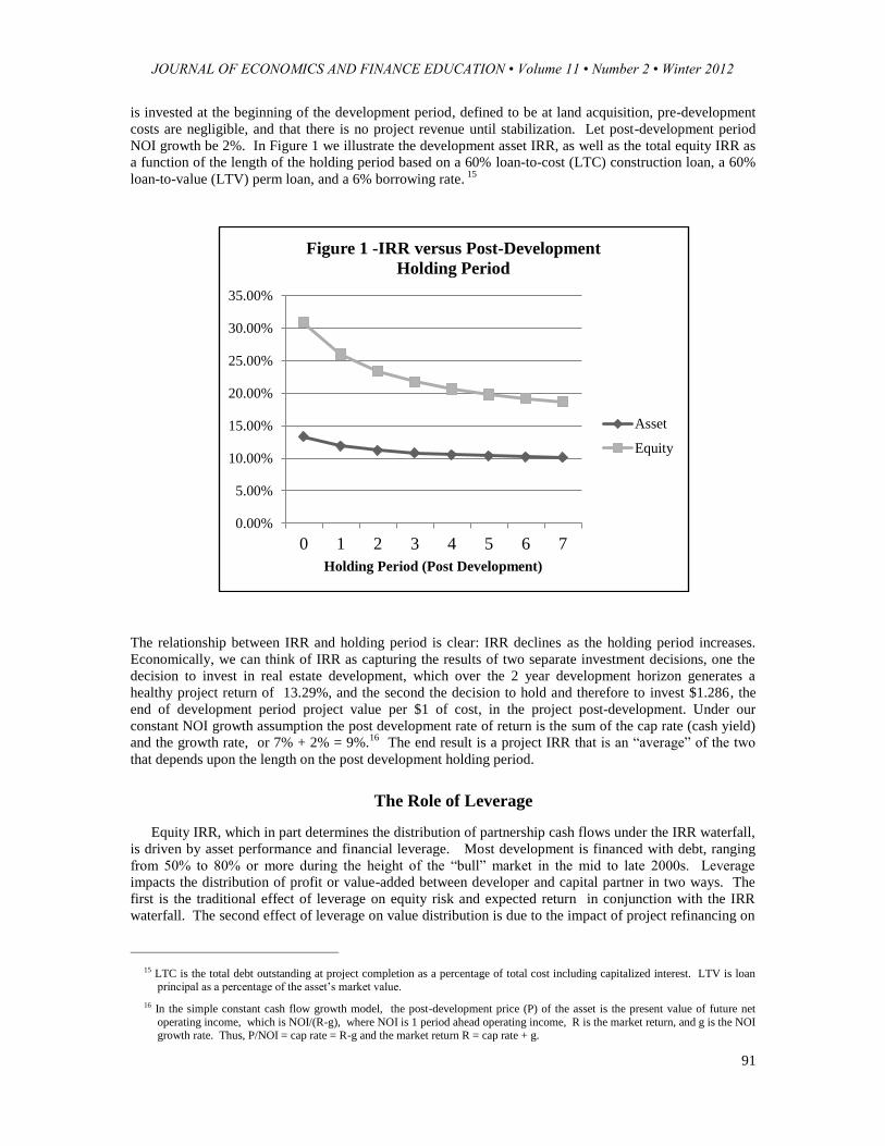
NOI growth be 2%. In Figure 1 we illustrate the development asset IRR, as well as the total equity IRR as

a function of the length of the holding period based on a 60% loan-to-cost (LTC) construction loan, a 60%

loan-to-value (LTV) perm loan, and a 6% borrowing rate. 15

The relationship between IRR and holding period is clear: IRR declines as the holding period increases.

Economically, we can think of IRR as capturing the results of two separate investment decisions, one the

decision to invest in real estate development, which over the 2 year development horizon generates a

healthy project return of 13.29%, and the second the decision to hold and therefore to invest $1.286, the

end of development period project value per $1 of cost, in the project post-development. Under our

constant NOI growth assumption the post development rate of return is the sum of the cap rate (cash yield)

and the growth rate, or 7% + 2% = 9%.16

The end result is a project IRR that is an “average” of the two

that depends upon the length on the post development holding period.

The Role of Leverage

Equity IRR, which in part determines the distribution of partnership cash flows under the IRR waterfall,

is driven by asset performance and financial leverage. Most development is financed with debt, ranging

from 50% to 80% or more during the height of the “bull” market in the mid to late 2000s. Leverage

impacts the distribution of profit or value-added between developer and capital partner in two ways. The

first is the traditional effect of leverage on equity risk and expected return in conjunction with the IRR

waterfall. The second effect of leverage on value distribution is due to the impact of project refinancing on

15 LTC is the total debt outstanding at project completion as a percentage of total cost including capitalized interest. LTV is loan principal as a percentage of the asset’s market value.

16 In the simple constant cash flow growth model, the post-development price (P) of the asset is the present value of future net

operating income, which is NOI/(R-g), where NOI is 1 period ahead operating income, R is the market return, and g is the NOI growth rate. Thus, P/NOI = cap rate = R-g and the market return R = cap rate + g.

0.00%

5.00%

10.00%

15.00%

20.00%

25.00%

30.00%

35.00%

0 1 2 3 4 5 6 7

Holding Period (Post Development)

Figure 1 -IRR versus Post-Development

Holding Period

Asset

Equity


92

the timing of the extraction of project profit. Depending on the relationship between construction debt

LTC and permanent debt loan-to-value LTV ratios, the refinancing of development debt at the end of the

development period allows the partnership to extract value-added prior to the final disposition of the

project, which will increase the project’s equity IRR. Assuming that perm debt LTV is at least as high as

construction loan LTC, the degree of “value extraction” depends on the LTV of the permanent loan. If

LTV and LTC are 70%, then 70% of the value-added is extracted on refinance. If perm loan LTV is higher

than construction loan LTC, then in addition to extraction of value-added, the joint venture can extract a

portion of its invested capital. The greater the extraction of cash on project completion, the greater will be

the equity IRR, apart from total project IRR.

Figure 2 captures Equity IRR as a function of the holding period for 60% and 80% debt ratios based on

the project parameters used in Figure 1 (a 9% development cap rate, 7% market cap rate, 2% annual NOI

growth, and 6% borrowing rate).

The 80% debt ratio equity IRR curve is considerably higher and somewhat steeper than the 60% curve, in

part a consequence of the fact that the return on equity is essentially the return on assets plus the product of

the debt to equity ratio and the asset return/debt yield spread. Although financial leverage most often

presents a value-neutral, risk-return tradeoff at the total equity level, to the extent that cash distribution

rules do not address leverage explicitly higher degrees of leverage could raise expected equity returns and

positively impact the developer’s share of equity cash and thus total wealth.

Risk, Return, and the Cash Flow Waterfall

As Kane (2001) points out, there is a spectrum of risk/return expectations across the universe of capital

partners. Opportunity funds pursue higher risks and returns than pension funds, and many other investors

lie in between. Investors use several mechanisms to manage risks. Obvious candidates include project

type and the degree of financial leverage employed. Alternative combinations of pref rates and promote

distribution parameters can be used to allocate risks between partners. Perhaps less obvious is the

investment holding period. Holding a development asset beyond the stabilization period is the equivalent of

investing in development, liquidating the asset and investing in a lower risk stabilized asset. The longer the

capital is invested in the stabilized asset, the lower the risk and return associated with the strategy over

0.00%

10.00%

20.00%

30.00%

40.00%

50.00%

60.00%

0 1 2 3 4 5 6 7

Holding Period (Post Devlopment)

Figure 2 - Leverage and Total Equity IRR

D = 60%

D = 80%


93

time. To the extent that the market for stabilized real estate assets is competitive, the degree of financial

leverage or the decision to hold the development asset beyond the development period will have little

impact on wealth creation. Yet both will impact equity IRR and potentially the shares of project cash flow

to the partners. Clearly, it is important to understand the relationships between strategic variables such as

investment horizon and the rules governing cash distribution, even when some of those strategic variables,

e.g., investment horizon, cannot be incorporated into the joint venture contract definitively. A corollary is

that the partners should understand each other’s strategic interests and those interests should be reflected in

the terms of the joint venture. Yet, based on observation developers are often unfamiliar with IRR math and

in many joint venture term sheets cash flow waterfall terms are free of any reference to either degree of

financial leverage or investment holding period.

Preferred Returns and IRR Thresholds

A defining characteristic of private capital markets is a lack of contract standardization. Although real

estate private equity investors often talk about “the” market preferred return (“pref”) rate, in practice there

are many. Pref rates under a standard pari pasu preferred return payment structure typically range from

7%-8% up to as much as 15%. Promote payment structures vary in degree of complexity. Payment rules

may involve one or several IRR thresholds. Contract terms will vary dependent on the experience of the

developer and the relative bargaining positions of the developer and capital partner. Common

development cap/market cap spread requirements of 200 bps.- 300 bps. tend to yield holding-period-

dependent asset IRRs of 10%-15% which when levered yield 20%-35% equity IRRs. Thus, preferred

return requirements are typically much lower than equity IRR based on spread targets, and developer

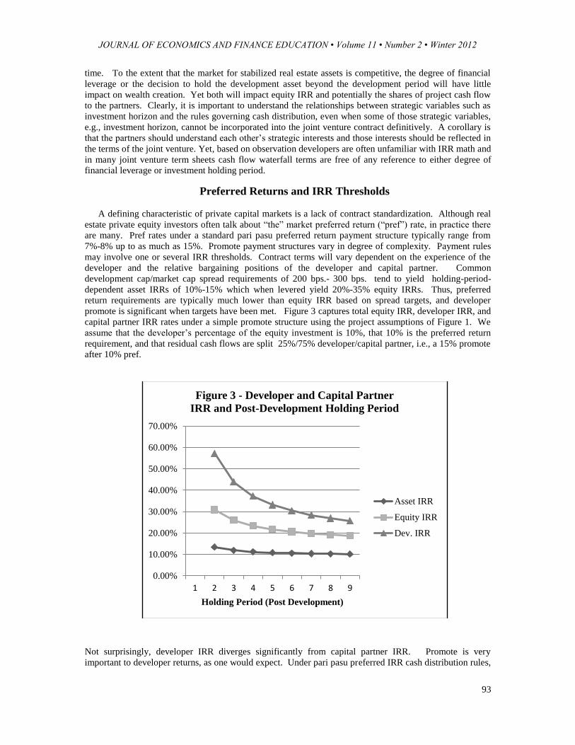
promote is significant when targets have been met. Figure 3 captures total equity IRR, developer IRR, and

capital partner IRR rates under a simple promote structure using the project assumptions of Figure 1. We

assume that the developer’s percentage of the equity investment is 10%, that 10% is the preferred return

requirement, and that residual cash flows are split 25%/75% developer/capital partner, i.e., a 15% promote

after 10% pref.

Not surprisingly, developer IRR diverges significantly from capital partner IRR. Promote is very

important to developer returns, as one would expect. Under pari pasu preferred IRR cash distribution rules,

0.00%

10.00%

20.00%

30.00%

40.00%

50.00%

60.00%

70.00%

1 2 3 4 5 6 7 8 9


Figure 3 - Developer and Capital Partner

IRR and Post-Development Holding Period

Asset IRR

Equity IRR

Dev. IRR


94

developer and capital partner IRR will diverge as long as levered total equity IRR is above the pref rate,

that is when the developer earns promote. Note that the relatively low IRR threshold for promote

payments afford a degree of protection to developers relative to project performance as well as the

potentially negative effects of holding period on promote payments. Figure 4 illustrates developer

(operating partner) IRR and total equity IRR as a function of post-development holding period over a range

of alternative preferred return rates. Debt, equity contribution, project performance assumptions, and cash

distribution rules (other than preferred return rate) are the same as in Figure 3.

Spreads between developer, capital partner, and total equity IRR decline as the holding period extends,

as one would expect. However, when pref rates are low developer IRR remains reasonably well above total

equity IRR over the entire modeled range. Under the pari pasu structure, when developer IRR and capital

partner IRR converge, developer promote must be zero. Since it is fair to assume that the decision to hold

the investment beyond the development period is essentially a zero NPV decision, the equity IRR curve

represents constant NPV values of IRR. The convergence of developer and equity IRR in high pref

environments signals a loss of net present value to the developer associated with extending the investment

horizon.

However, when pref requirements are relatively low developer IRR does not converge on equity IRR

over our hypothetical investment horizon. Therefore, we can’t conclude that developer NPV declines over

time based on IRR alone. In order to directly estimate the effects of the investment horizon on developer

NPV, we compute the present value of the developer’s position as a function of the post-development

holding period under alternative pref values. We use the same compensation structure as the model above.

The model assumes a constant 2% NOI growth rate and that the completed project is priced to a 7% cap

rate, thus the required return on the asset is 9%. At a 60% initial loan-to-value ratio and 6% permanent

debt rate, the initial required (market) equity return is .09 + (.6/.4) x (.09-.06) = 13.5% . Note that under

the constant cash flow growth model asset value grows at 2% per year and the leverage ratio and discount

rate decline marginally over time.

Figure 5 illustrates the relationship between developer wealth and post-development investment horizon

over a range of pref rates from 10% to 25%.

0.00%

10.00%

20.00%

30.00%

40.00%

50.00%

60.00%

70.00%

1 2 3 4 5 6 7 8 9


Figure 4 - Developer IRR versus Holding

Period for Alternative Pref Rates

5%

10%

15%

20%

25%

Equity


95

As expected, at high pref rates developer wealth declines with the length of the investment horizon, and the

effect is meaningful. At 20% pref, the developer’s loss of value over the investment horizon is more than

20%. Surprisingly, at low pref rates developer wealth is marginally increasing in the investment horizon,

despite the general effects of investment horizon on equity IRR. Pref rates are applied to cash equity

investment. Given the relatively high required returns on total development equity, the carrying value of

equity (investment plus accrued preferred returns over the development period) is much smaller than the

market value of that equity at successful completion of the project. In addition, pref rates are often smaller

than the required equity return in the post development period. In these lower pref rate environments

operating cash flows and price appreciation, which are just sufficient to provide the required return on the

market value of equity, are much higher than necessary to meet the preferred return on the carrying value of

equity. Distributions are skewed toward higher promote payments that increase the present value of the

developer’s position.

Distribution of Development Value-Added

So far we have considered the effects of post-development investment horizon on wealth distribution.

Apart from the impact of the investment horizon, it is useful to understand how the IRR waterfall

distributes total development project net present value. Unfortunately, there is no perfect way to answer

this because we have no price data with which to estimate the required return on real estate development.

Indirectly, we can use development cap/market cap spreads to estimate required asset IRR for a given

development period. The hybrid nature of real estate private equity and the differential residual positions

held by the developer and the capital partner make the required equity return more difficult. For typical

pref rates and required spreads, significant promote payments will result in a divergence between developer

IRR, capital partner IRR, and the total equity IRR. This divergence will be driven by the specifics of the

waterfall, which are likely to be at least somewhat independent of the risks of the project. As a starting

point, we take the capital partner’s IRR at the required spread and given waterfall structure as the required

equity return. As before, assume a 2% spread (7% market cap, 9% development cap) and 24 month

development period, 10% equity investment by the developer, and 10% pref with 75%/25% cash flow

splits after pref. We compute developer/capital partner NPV for a range of realized development

cap/market cap spreads as of the end of the development period. Figure 6 captures developer/capital

0.00%

2.00%

4.00%

6.00%

8.00%

10.00%

12.00%

1 2 3 4 5 6 7 8


Figure 5 - Developer Present Value

as % of Project Cost

25% pref

20% pref

15% pref

13% pref

10% pref


96

partner net present value for spreads ranging from 2%-4%. By definition, the capital partner’s NPV is 0

when the spread is 2%.

Using the capital partner’s IRR at the 2% spread as the discount rate results in positive NPV for the

developer given the yield differentials created by promote payments, which accrue when projects are

breakeven for the capital partner. Relative to total project costs capital partner NPV grows more rapidly as

performance improves, reflecting the capital partner’s much larger investment. However, it can be shown

that NPV per dollar invested in much higher for the developer across the range, reflecting the developer’s

large relative residual interest.

Teaching Joint Venture Economics

Real estate development private equity can be covered in an upper level undergraduate or graduate real

estate capital markets course. Some students will have been exposed to private equity structures, however

many will not. We begin with the basics of private equity funds and then move to joint ventures. Because

the nature of private equity is much different than public common equity, the mechanics of cash

distribution rules will be foreign to most and it is a good idea to provide a number of relatively simple

examples. We start with private equity distribution rules in one-period investment horizons. As noted,

funds often pay carried interest on accounting profit subject to the requirement that investors earn at least

their preferred return. Some funds are more restrictive and pay carried interest only on residual cash flow

after pref and return of capital, essentially the pari pasu rule most commonly used in joint ventures. An

intermediate position requires pari pasu splits until the preferred return hurdle has been met, but then a

much higher “catch-up” operating promote split until a the targeted percentage of the total profit has been

reached. Single period investment examples, analogous to the 24 month example found in the discussion

of cash distribution rules above, are easy to produce. For instance, when comparing the hard IRR

requirement before promote against the accounting profit standard, all that is required is a one-period

project that earns significantly above the pref rate.

In addition, illustrations involving American versus European waterfall structures within a fund can be

used to illustrate cash flow timing issues and the impact of diversification. Under the hard preferred IRR

standard, promote/carried interest is paid only after the preferred IRR has been met. When there are

multiple projects, one or more of which fail to meet the preferred IRR, the poorly performing do not

0

0.02

0.04

0.06

0.08

0.1

0.12

0.14

2 2.5 3 3.5 4

Development Cap/Market Cap Spread (%)

Figure 6 - Developer/Capital Partner NPV per $

of Project Cost

Developer

Cap Partner


97

impact promote/carried interest payments on successful projects under an American waterfall, in which the

distribution rule is applied to each project sequentially. However, in applying the rule to the aggregate

investment under the European structure some of the “excess” IRR from the successful projects has to be

allocated to the unsuccessful projects before any promote/carried interest is paid. A one-period, two

project fund with differential project IRRs which when aggregated earn exactly the pref rate on total equity

can be used to illustrate this. Consider simultaneous 24 month development projects each with $60 million

in total costs (including capitalized interest) financed with $20 million in equity. Both projects are initially

forecast to earn a 10% development cap rate (yield on cost) at completion. The market cap rate is assumed

to be 8.5%. Let one project reach its 10% development cap, but suppose that the other project earns 8.44%

on cost and thus falls marginally short of the market cap rate. Assume that the projects are liquidated on

completion and that no cash is received before liquidation. The sales proceeds from the liquidation of the

10% development cap project are $60 x (.10/.085) = $70.59. Net of $40 in debt the equity investors receive

$30.59. For the lower yielding project, sale proceeds are $60 x (.0844/.085) = $59.59. Net of debt, equity

holders receive $19.59. Total equity cash flow = $50.18. Let the equity investment percentages be 10%

operating partner, 90% capital partner. Consider a cash distribution rule with pari pasu payments until a

12% IRR has been reached and 25%/75% operating partner/capital partner distribution thereafter. Under a

European waterfall the cash distribution rule is applied to total equity investment of $40 million. The

preferred IRR requirement = $40 x (1.12)2 = $50.18. Thus proceeds are just sufficient to meet the preferred

return requirement and all cash flow is distributed pari pasu. The operating partner will receive 10% or

$5.018. Under an American waterfall, the cash distribution rule is applied sequentially. For each project,

$20 x (1.12)2 = $25.09 is the preferred return requirement. Cash flow from the higher yielding project is

split 90/10 until the first $25.09 has been paid out, and then promote payments are earned on the remaining

$5.50. Thus the operating partner receives $25.09 x .10 + $5.50 x .25 = $3.884. The second project does

not pay out enough cash to reach the IRR requirement, and thus the entire distribution is pari pasu so that

the operating partner receives $19.59 x .1 = $1.959 from this investment. The operating partner receives

$5.843 in total. Relative to the European waterfall, the operating partner receives an extra amount

corresponding to the promote payment on the higher yielding project, .15 x ($5.50) = $.825, at the expense

of the capital partner.

We then consider cash flows over multiple period investments under the common pari pasu/promote

cash distribution structure that, as described, is equivalent to the restrictive fund waterfall. One of the

advantages of this structure is that the pref requirements under these cash distribution rules behave as

cumulating preferred stock. Spreadsheets are invaluable in these exercises, and in order to determine which

cash flows are required to pay pref before splits change, we would recommend creating a basic template in

which you track equity investment inclusive of cumulating preferred return and net of equity cash flows

received. (See the appendix.) In order to talk about joint ventures in real estate development, it is best to

introduce the development cap and the spread as the set of project feasibility metrics early and to connect

them to IRR with illustrations. The risk-return profile of real estate development can be illustrated with

exercises in which shocks to the development cap rate or the development horizon are translated into IRR.

For instance, a simple example might involve a development project originally forecast to reach

stabilization (construction completion and lease-up) in 24 months for which lease-up takes 36 months.

Under these circumstances, the construction loan will need to be extended by twelve months, and total

project costs, will increase by a year’s worth of interest. If we assume that cash inflows are lagged by 12

months but that NOI and the market cap rate are otherwise consistent with the original forecast, we can

compute IRR simply as in the examples above. The impact of this sort of project risk on realized return is

usually quite significant.

Although students are exposed to the distinction between wealth creation and rate of return typically in

their first finance class, it often does not fully register. Unfortunately, the issues related to cash distribution

rules, pref rates, IRR, and NPV are difficult, and the deeper ones are likely to be beyond many

undergraduates, so that pursuing them may be counterproductive. None the less, we have found that having

students work through the mechanics of the distribution rules and interpreting the results is a good exercise.

We do this in the context of a case study involving a developer that during the height of the commercial

real estate boom was pursued by 2 potential capital partners for the opportunity to invest in a Hawaiian

retail development. The term sheets for the two potential joint ventures were markedly different, one

offering a considerably more developer-friendly waterfall and the other offering a considerably more

seasoned capital partner, which was significant given that the development firm was reasonable

inexperienced. Students are asked to model the developer’s position under each structure for a “good” and


98

“bad” project scenario (defined in terms of development cap/market cap spreads), and to choose a capital

partner based on the economics of the respective joint ventures as well as the risks associated with

inexperience. An in-class discussion of results can be illuminating and is recommended.17

References

Brueggeman, William and Jeffrey Fisher. Real Estate Finance and Investments 14e., (2011), New York,

NY: McGraw-Hill Irwin.

Federal Reserve Bank of San Francisco. Economic Letter, (2008), February.

Kane, Meredith, “Equity Investment in Real Estate Development Projects: A Negotiating Guide for

Investors and Developers,” The Real Estate Finance Journal, (Spring 2001), 1-13.

Kaplan, Steve and Schoar, Antoinette (2005), “Private Equity Performance: Returns, Persistence, and

Capital Flows,” Journal of Finance, (2005 Vol. 60 No. 4), 1791‐1823.

Koufopoulos, Kostas (2007), “Managerial Compensation and Capital Structure under Asymmetric

Information,” University of Warwick - Finance Group Working Paper Series, (2007).

Kuzmicki, Andrae and Daniel Simunac (2008), “Private Equity Real Estate Finds: An Institutional

Perspective,” Real Property Association of Canada.

Linneman, Peter, Real Estate Finance and Investments: Risks and Opportunities 2e, Linneman

Associates, (2004), Philadelphia, PA.

Metrick, Andrew and Ayako Yasuda, “The Economics of Private Equity Funds,” Review of Financial

Studies, (2010 Vol. 23), 2303-2341.

Private Equity Council, “Public Value: A Primer on Private Equity,” (2007), Research Report.

Tomperi, I, “Performance of Private Equity Real estate Funds,” (May 2009), Unpublished Manuscript.

Robinson, David and Berk Sensoy, “Do Private Equity Managers Earn Their Fees? Compensation,

Ownership, and Cash Flow performance,” NBER Working Paper Number 17942, March 2012.

17 A summary of the case study and a short solution key are available from the author upon request.

http://papers.ssrn.com/sol3/cf_dev/AbsByAuth.cfm?per_id=358994

http://papers.ssrn.com/sol3/papers.cfm?abstract_id=996334


99

Appendix - Cash Flow/IRR Computations

Asset Cash Flow and IRR

Consider a 24 month real estate development project whose development cap rate, NOI/cost, is

forecast to be 9% and for which NOI grows at 2% post development. Let the current and near-term

forecasted market cap rate, (NOI)/(market price), be 7%. For simplicity assume that all project costs are

incurred at the beginning of the project, no revenue is received until the end of the development period, and

that cash receipts happen at the end of each year. Per $1 of cost, $1 is invested immediately and operating

cash flow forecasts are $.09 in year 3, growing at 2% each year thereafter. The forecasted market value of

the development asset at the end of each period can be found from the market cap rate. Since the market

cap is NOI/price, price = NOI/(market cap). If the market cap forecast is fixed at 7%, the value of the

development per $1 of project cost at the end of the development period is $.09/.07 = $1.286 and it grows

at 2% per year. Table 1 captures total cash flow per $1 of project cost and IRR for project holding periods

of 2-5 years.

Table 1 – Cash Flow per $1 Cost and Project IRR

Year 0 1 2 3 4 5

Investment -1 0 0 0 0 0

Oper.Incom

e

0.09 0.0918 0.093636

Market

Value

1.285714 1.311429 1.337657 1.36441

CF IRR

2 Yrs. -1 0 1.285714 0 0 0 13.39%

3 Yrs. -1 0 0 1.401429 0 0 11.91%

4 Yrs. -1 0 0 0.09 1.429457 0 11.21%

5 Yrs. -1 0 0 0.09 0.0918 1.458046 10.80%

Total Equity Cash Flow and IRR

Suppose that our simple project is financed with construction debt and that the loan-to-cost ratio,

defined as end of project loan balance relative to total costs including capitalized interest, is 60%. In the

event the real estate asset is held beyond the development period, assume that the development loan is

refinanced with perm debt and that the loan-to-value ratio of the perm loan is also 60%. Note that a

successful project will generate significant value-added (market value net of total cost), and that refinance

is an avenue for extracting a portion of that value-added. In our illustration project market value post

development is $1.286 (approx.) per $1 of cost. A 60% loan-to-value perm loan generates $1.286 x .60 =

$.772, leaving $.172 (60% of value-added) after paying off the construction loan balance. In contrast to

construction debt, perm debt interest is paid in cash rather than capitalized. Table 2 represents total end-

of-period equity cash flow and IRR based on a perm debt interest rate of 6%:


100

Table 2 – Total Equity Cash Flow and IRR

Year 0 1 2 3 4 5

Equity Inv. -0.400 0.000 0.000 0.000 0.000 0.000

Oper.Income 0.090 0.092 0.094

Interest 0.077 0.077 0.077

Market Value 1.286 1.311 1.338 1.364

Debt 0.771 0.771 0.771 0.771

Residual Value 0.514 0.540 0.566 0.593

Refinance CF 0.171

Equity CF IRR

2 Yrs. -0.400 0.000 0.686 31%

3 Yrs. -0.400 0.000 0.171 0.540 23%

4 Yrs. -0.400 0.000 0.171 0.013 0.566 20%

Residual value in Table 2 is simply asset market value net of debt and is the equity portion of asset sales proceeds. Total equity cash

flow in any period is operating income net of interest payments, net refinance cash flow, and residual value in the last year of the

holding period.

Equity Cash Flow Splits

Let 10% of the equity investment in our simple project come from the developer/operating partner and

the remaining 90% from a capital partner. The cash flow waterfall is assumed to be pari pasu distribution

until a 12% IRR has been earned on equity capital, with 75% capital partner/25% operating partner splits

thereafter. Table 3 provides these cash splits and investor IRRs assumed a 5 year total project life (3 year

post development holding period).

Table 3 Equity Cash Flow Splits – 3 Year Post-Development Holding Period

Year 0 1 2 3 4 5

Acct. Bal. 0.400 0.448 0.502 0.370 0.400 0.432

Cash Flow 0.000 0.171 0.013 0.015 0.593

Net Bal. 0.448 0.330 0.357 0.385 -0.161

Cash Splits IRR

Op. Partner -0.040 0.000 0.017 0.001 0.001 0.084 25%

Cap. Partner -0.360 0.000 0.154 0.012 0.013 0.509 17%

The top line in Table 3 in the prior period’s equity (net) balance plus that period’s 12% preferred return. Equity cash flow is netted

from this line to give the net preferred account balance to be carried forward. Cash flow is distributed pari pasu until the net balance is ≤ 0, that is until the preferred IRR has been met. A negative net balance represents cash flow that is distributed 25%/75%, i.e., cash

flow over which the operating partner receives promote payments.

understanding and teaching private equity structures ... · this paper is intended to serve as a...

Documents