under-investment in profitable technologies when...

Under-investment in Profitable Technologies when Experimenting is Risky: Evidence from a Migration Experiment in Bangladesh

Gharad Bryan, London School of Economics

Shyamal Chowdhury, University of Sydney A. Mushfiq Mobarak, Yale University*

*Contact Author: [email protected], 203-432-5787

April 1, 2011

Preliminary and Incomplete

Abstract The rural north-western districts of Bangladesh, home to 10 million people, experience a pre-harvest

seasonal famine, locally known as Monga, with disturbing regularity. Inspired by the observations that wages are higher, jobs are more plentiful in nearby urban areas than in the monga-prone region, and that there are no official restrictions on mobility, we provide monetary incentives in 100 study villages to encourage people to seasonally migrate out in search of employment. We employ a randomized intervention design to study the patterns of responsiveness to our incentives using a 1900 household sample, which illuminates the current constraints to seasonal out-migration. The randomization also allows us to cleanly estimate the (causal) returns to migration in terms of household expenditures, savings and earnings, and caloric intake.

The propensity to seasonally out-migrate is very responsive to a 600-800 Taka cash/credit incentive, raising the migration rate to 57%, relative to 34% in a set of control villages. Simply providing information on job availability and wages at destination has no effect on the migration rate. Comparing the characteristics if migrants in the treatment and control areas, the incentives appear to induce people who otherwise feel less comfortable migrating – i.e. those without job leads or social network presence at the destination, and new migrants. Households closer to subsistence are less likely to migrate, but are much more responsive to the incentive.

The migrant experience was very successful on average: monthly consumption increased by at least Tk 300 ($4) per person per month, or Tk 1050 ($15) per household per month due to the induced migration. Earnings, savings and remittances from each migration episode are several multiples of the initial investment (the incentive, or the round-trip cost of moving). Most strikingly, migration rate in the treatment areas remained significantly higher in the treatment areas (47% vs. 35%) a year after the program, even after all incentives are removed. Induced migration in one year increases the propensity to re-migrate by 40 percentage points. There is evidence of learning among induced migrants, such as a greater propensity to re-migrate when the initial migration episode was more successful, greater growth in savings/earnings per day in treatment group, and larger consumption effect in 2009 among re-migrants.

These results are consistent with a model of a migration-based poverty trap, where individuals are uncertain about their own prospects at the destination, and particularly worried about a bad outcome (e.g. undertaking the costs of moving, but then not finding a job) during a period in which their family is under the threat of famine. The uncertainty associated with migration prevents households from investing, even when the expected returns are positive. Our intervention insures households against the bad outcome, thereby allowing them to invest, learn about their private returns to the investment, and for those with positive realizations, re-migrate the next period even in the absence of the intervention. Many of the empirical results are also consistent with a simple model of a liquidity/credit constraint preventing migration.

These results suggest that a grant program, or a credit program with limited liability (which amounts to insuring households against the possibility of a bad outcome) is likely to be welfare enhancing, and can be an effective policy response against the threat of localized seasonal famines such as Monga. More broadly, providing small grants or credit that enable households to search for jobs, and leads to a better spatial and seasonal matching between potential employers and employees may be a useful complement to the much-more-popular microcredit programs that aim to create new entrepreneurs and new businesses.

Underinvestment in Profitable Technologies when

Experimenation is Costly:

Evidence from a Migration Experiment In Bangladesh

Gharad Bryan, Shyamal Chowdhury and A. Mushfiq Mobarak

April 1, 2011

1 Introduction

The causes and consequences of internal migration have received comparatively little attentionin the economics and policy literatures, even though it is much more common than the heavily-studied issue of international migration (Borjas 1999, Rosenzweig 2005, Yang 2008, Hanson2009). There were 240 times as many internal migrants in China in 2001 as there were inter-national migrants (Ping 2003), and 4.3 million people migrated internally in the 5 years leadingup to the 1999 Vietnam census compared to only 300,000 international migrants (Ahn et al,2003). The development effects of internal migration are arguably more profound: the majorityof households in rural Rajasthan migrate seasonally in search of employment, and use this asthe primary vehicle for diversifying sources of income (Banerjee and Duflo 2006).

This paper studies the causes and consequences of internal seasonal migration in north-western Bangladesh, in a region where over 5 million people below the poverty line must copewith a pre-harvest seasonal famine, known locally as Monga, almost every year (The DailyStar 2010). This seasonal famine is emblematic of widespread pre-harvest “lean” or “hungry”seasons throughout South Asia and Sub-Saharan Africa documented in a number of studies,1

where imperfect consumption smoothing forces households below poverty during parts of theyear. Inspired by the observation that nearby urban areas offer better wage and employment op-

1Seasonal poverty or hungry seasons have been documented in Ethiopia (Dercon and Krishnan 2000, who showthat poverty and malnourishment increase 27% during the lean season), Malawi (Brune et al 2010), Madagascar(Dostie et al 2002, who estimate that 1 million people fall below poverty before the rice harvest), Kenya (Swift 1989,who distinguishes between years that people died versus years of less severe shortage), Thailand (Paxson 1993),India (Chaudhuri and Paxson 2002) and China (Jalan and Ravallion 1999).

1

portunities during the lean season, we provide small grant and loan incentives (of $8.50 or 600Taka) in 100 study villages to encourage people to seasonally migrate out in search of employ-ment. The random assignment of incentives allows us to generate among the first experimentalestimates of the effects of migration, and internal migration in particular.Estimating the returnsto migration is the subject of a very large literature, but one that has been hampered by diffi-cult selection issues (Akee 2010, Grogger and Hanson 2010, McKenzie et al 2010). The internalseasonal migration we encourage is a commonly used means to cope with seasonal povertyand natural disasters across Asia, Africa and Latin America,2 and our estimates of the effects ofmigration thus have substantial external relevance.

We estimate the causal effects of being induced to migrate away during the lean season tobe very large.These estimates add to an emerging literature that documents very high ratesof return to small capital investments in developing countries (Udry and Anagol 200x, De Mel,McKenzie and Woodruff 200x and 200x and Duflo, Kremer and Robinson 2009), and bolsters thecase made by Clemens and Pritchett (20xx), Rosenzweig and xx (200x) and Gibson and McKen-zie (2010) that offering migration opportunities improves welfare by much more than any otherdevelopment intervention in health, education or agriculture that has been studied. Migrationinduced by our intervention increases food and non-food consumption of the migrants familymembers remaining at the origin by 30-35%, and improves their caloric intake by 700 caloriesper person per day. On an initial investment of about $6-$8 (the average round-trip cost to adestination), migrants earn $110 on average during the lean season and save about half of that,which are suggestive of a very high rate of return on investment.Most strikingly, these inducedmigrants continue to re-migrate at a higher rate compared to a control group a year later, evenafter the inducement for migration is removed.These large positive returns, consumption effectsand preferences revealed by the voluntary re-migration beg one very important question: Whydidn’t these people already engage in such a highly profitable investment?

To understand this puzzling behavior, we propose a model in which experimenting witha new technology or behavior such as migrating to a new destination - is risky, and rationalhouseholds do not migrate in the face of uncertainty about their prospects at the destinationeven when they expect monetary returns to the activity to be positive. This results in a povertytrap in which households do not migrate out of fear of an unlikely, but devastatingly negativeoutcome where they undertake the cost of moving but return hungry after not finding employ-ment during a period when their family is under the threat of famine. Inducing the inaugural

2Prior attempts use controls for observables (Adams 1998), selection correction methods (Barham and Boucher1998; Acosta et al 2007), instrumental variables methods (BenYishay 2010, McKenzie and Rapoport 2007, Brown andLeeves 2007, Yang 2008) and natural policy experiments (Clemens 2010, Gibson et al 2010) to answer this question.

2

migration by insuring against this devastating outcome which our grant or loan with impliedlimited liability managed to do can lead to long-run benefits where households either learn howwell their skills fare at the destination, or improve their future prospects by allowing employersto learn about them. This simple model can explain the high take-up rate for the intervention,the large positive income and consumption effects, and the greater re-migration in a future pe-riod among treatment households even after the inducement is removed.

The proposed model also makes four other predictions regarding migration behavior. First,households that are close to subsistence – on whom experimentation with the new technologyimposes the biggest risk – should be less likely to migrate and more likely to benefit from ourintervention. Second, households that do not know someone at the destination and thereforedo no have the contacts necessary for successful migration should be less likely to migrate andmore likely to respond to our incentive. Third, because the poverty trap is generated by thepossibility of a large negative return and that possibility can be effectively mitigated through aloan that does not have to be paid off if the migration episode was not successful, we predict thatcash and credit incentives should have roughly the same effect on the migration rate. Fourth,the possibility of learning implies that those households that are most successful should bethose most likely to repeat migrate and that repeat migration will be to the same location asprior migration. We find support for all of these conclusions in our data, the last one tested byusing additional exogenous variation in migration location induced by conditionalities placedon migration in our experiment.

Households reluctance to engage in risky or costly experimentation can provide insight intoa number of other important puzzles in growth and development. Green revolution technolo-gies led to dramatic increases in agricultural productivity in South Asia (Evenson and Gollin2003), but take-up and diffusion of the new technologies was surprisingly slow, partly due tolow levels of experimentation and the resultant slow learning (Munshi 2004). More directly,research has linked the inability to experiment due to uninsured risk to a bias towards lowrisk low-return technologies that stunt long-run growth (Yesuf et al 20xx), and to reduced in-vestments in agricultural inputs and technologies such as new high-yield variety seeds andfertilizer (Rosenzweig and Wolpin 1993a, Dercon and Christiansen 2009). Aversions to exper-imentation can also hinder entrepreneurship and business start-ups and growth (Hausmannand Rodrik 2003; Fischer 2009), and can force sales of productive investment assets in order tosmooth consumption (Rosenzweig and Wolpin 1993b). We contribute to this literature by usingexperimental variation in data to build evidence on the presence of a poverty trap induced byinefficiently low levels of experimentation.

3

Our model and experimental results shed light on a fundamental puzzle in developmenteconomics, which is that adoption rates of highly efficacious technologies with the potential toaddress important development challenges - ranging from tropical diseases to low agriculturalproductivity to low rates of savings and investment - have remained surprisingly low (Millerand Mobarak 2010, Null et al 2010). If adoption is risky (e.g. due to risk of crop failure, or uncer-tainty about durability of a new stove or water purifying technology) then giving householdsthe opportunity to experiment with the new technology by insuring against failure may be aneffective marketing strategy.

Finally, from a narrow policy perspective, our experiments uncover a cost-effective responseto the widespread famines that afflict the 10 million people residing in Rangpur region ofBangladesh with disturbing regularity. Such lean seasons are not phenomena unique to north-western Bangladesh: there is a predictable pre-harvest hungry season every year in Malawi,Ethiopia, Madagascar and other countries, forcing millions to succumb to seasonal poverty. Thesolution we implement is inexpensive (the vast majority repay the $8.50 inducement when it isoffered as a loan), it confers long-run benefits even when offered as a one-off, and it is more sus-tainable than subsidizing food purchases on an ongoing basis, which is the major anti-faminepolicy tool currently employed by the Bangladesh government (Khandker 2010; Governmentof Bangladesh 2005, journalistic cite). Our intervention mitigates the spatial mismatch betweenwhere people are based, and where the jobs and excess demand for labor are during the pre-harvest months. This approach may be of relevance to other countries that face geographicconcentrations of poverty, such as northern Nigeria, eastern islands of Indonesia, northeast In-dia, southeast Mexico, and inland southwest China (Jalan and Ravallion 2002). Of course onehas to be careful about general equilibrium effects at the destination when such a program isscaled up, but instances of excess labor demand during particular seasons is not altogether un-common even in developing countries. Our findings suggest that providing credit to enablehouseholds to search for jobs, and aid spatial and seasonal matching between potential employ-ers and employees may be a useful way to augment the microcredit concept currently morenarrowly focused on creating new entrepreneurs and new businesses.

The next two sections describe the context and the design of our interventions. We presentresults on program take-up and the effects of migration in Section 4. These findings motivatethe risky experimentation model in Section 5. We present statistical tests of various implicationsof the model in section 6, discuss alternative explanations of the data in Section 7 and offerconclusions and policy advice in section 8.

4

2 The Context: Northwestern Bangladesh and the Monga Famine

Our experiments are conducted in 100 villages in two districts (Kurigram and Lalmonirhat)in the seasonal-famine prone Rangpur region of north-western Bangladesh. The Rangpur re-gion is home to roughly 7% of the countrys population, or 9.6 million people. 57% of the re-gions population (or 5.3 million people) live below the poverty line.3 In addition to the levelof poverty, the Rangpur region experiences more pronounced seasonality in income and con-sumption, with incomes decreasing by 50-60% and expenditures on food dropping by 10-25%during the post-planting and pre-harvest season (September-November) for the main Amanrice crop (Khandker 2010). As Figure 1 indicates, the price of rice also spikes during this sea-son, particularly in Rangpur, and thus kilos of rice consumed drops 22% even as householdsshift monetary expenditures towards food (Figure 2) while waiting for the Aman rice harvest.The lack of job opportunities and low wages during the pre-harvest season and the coincidentincrease in grain prices combines to create a situation of seasonal deprivation and famine (Mah-mud and Khandker 20xx, Sen 1981)4. The famine occurs with disturbing regularity and thushas a name Monga. It has been described as a routine crisis (Rahman 1995), and its effects onhunger and starvation widely chronicled in the local media. Agricultural wages in the Rangpurregion are already among the lowest in the country over the entire year (BBS Monthly StatisticalBulletins), and further, demand for agricultural labor plunges between planting and harvest.The resultant drastic drop in purchasing power for Rangpur households reliant on agriculturalwage employment takes (or threatens to take) consumption below subsistence.

[Figure 1 about here.]


Several puzzling stylized facts about household and institutional characteristics and cop-ing strategies motivate the design of our migration experiments. First, seasonal out-migrationfrom the monga-prone districts appears to be low despite the absence of local non-farm employ-ment opportunities. According to the nationally representative HIES 2005 data, only 5 percentof households in Monga prone districts receive domestic remittances, while 22 percent of all

3Extreme poverty rates (defined as individuals who cannot meet the 2100 calorie per day food intake even ifthey spend their entire incomes on food purchases only) were 25 percent nationwide, but 43 percent in the Rangpurdistricts. Poverty figures are based on Bangladesh Bureau of Statistics (BBS) Household Income and expendituresurvey 2005 (HIES 2005), and population figures are based on projections from the 2001 Census data.

4Amartya Sen (1981) notes these price spikes and wage plunges as important causes of the 1974 famine inBangladesh, and that the greater Rangpur districts were among the most severely affected by this famine.

5

Bangladeshi households do. Remittances generally under-predict out-migration rates, but thesize and direction of this gap (lower migration out of the poorest district) are still puzzling. Itis more common for agricultural laborers in other regions to migrate in search of higher wagesand employment opportunities, and this is known to be one primary mechanism by whichhouseholds diversify income sources in India (Banerjee and Duflo 2006).

Second, inter-regional variation in income and poverty between Rangpur and the rest ofthe Bangladesh have been shown to be much larger than the inter-seasonal variation withinRangpur (Khandker 2010). This suggests smoothing strategies that take advantage of inter-regional variation (i.e. migration) rather than inter-seasonal variation (e.g. savings, credit) mayhold greater promise. Moreover, an in-depth case-study of the Monga phenomenon (Zug 2006)explicitly notes that there are off-farm employment opportunities in rickshaw-pulling and con-struction in nearby urban areas during the monga season. To be sure, Zug 2006 points outthat this is a risky proposition for many, as labor demand and wages drop all over rice-growingBangladesh during that season. However, this seasonality is less pronounced than that observedin Rangpur (Khandker 2010).

Finally, both government and large NGO monga-mitigation efforts have concentrated on di-rect subsidy programs like free or highly-subsidized grain distribution (e.g. “Vulnerable GroupFeeding,”), or food-for-work and targeted microcredit programs. These programs are expen-sive, and the stringent micro-credit repayment schedule may itself keep households from en-gaging in profitable migration (Shonchoy 2010). There are structural reasons associated withrice production seasonality for the seasonal unemployment in Rangpur, and thus encouragingseasonal migration towards where jobs are appears to be a sensible complementary policy toexperiment with.

3 Design of Interventions and Experiment

The two districts where the project is conducted (Lalmonirhat and Kurigram) represent theagro-ecological zones that regularly witness the monga famine (World Bank Umar cite). Werandomly selected 100 villages in these two districts and first conducted a village census ineach location in June 2008. Next we randomly selected 19 households in each village fromthe set of households that reported (a) that they owned less than 50 decimals of land, and (b)that a household member was forced to miss meals during the prior (2007) monga season. Weconducted a baseline survey of these 1900 households during the pre-monga season in July2008.

6

In August 2008 the researchers randomly allocated the 100 villages into four groups: Cash,Credit, Information and Control using a pure random number generator in Stata. These treat-ments were subsequently implemented in collaboration with PKSF5 and their NGO partnerorganizations with field presence in the two chosen districts. We trained the NGOs on the im-plementation procedure in August 2008, and they implemented the interventions during the2008 Monga season starting in September. 16 of the 100 study villages (consisting of 304 samplehouseholds) were randomly assigned to form a control group. A further 16 villages (consist-ing of another 304 sample households) were placed in a job information only treatment. Thesehouseholds were given information on types of jobs available in four pre-selected destinations,the likelihood of getting such a job and approximate wages associated with each type of joband destination. 703 households in 37 randomly selected villages were offered cash of Taka 600(∼US$8.50) at the origin conditional on migration, and an additional bonus of Taka 200 (∼US$3)if the migrant reported to us at the destination during a specified time period. We also providedexactly the same information about jobs and wages to this group as in the information-onlytreatment. Taka 600 covers a little more than the average round-trip cost of safe travel from thetwo origin districts to the 4 nearby towns on which we provided job and wage information. The589 households in the final set of 31 villages were offered the same information and the sameTk 600 + Tk 200 incentive to migrate, but in the form of a zero-interest loan to be paid back atthe end of the monga season (in December) rather than a cash grant.

In the 68 villages where we provided monetary incentives for people to seasonally out-migrate (37 cash + 31 credit villages), we sometimes randomly assigned additional condition-alities to different households within the village. For example, 12 of the 19 households wererequired to migrate in groups, and specific group members were assigned in half the case. Also,about half the households were required to migrate to a specific destination. We will not directlyanalyze the effects of such conditionalities in this paper, but these conditionalities were helpfulin creating random within-village variation in specific households propensity to migrate. Thisrandom variation will be useful for some of the empirical analysis presented later. Figure 8provides an overview of the randomized intervention conditions.

5PKSF (Palli Karma Sahayak Foundation) is an apex micro-credit funding and capacity building organizations inBangladesh. It is a company not for profit set up by the Government of Bangladesh in 1990, for poverty alleviationthrough the provision of micro-credit through its Partner Organisations (POs).

7

4 Returns to Seasonal Migration

In this section we report simple “program evaluation” results on take-up of the treatment, theeffects of seasonal migration on the households consumption and welfare at the origin, incomeand savings of the migrant at the destination, and the propensity to re-migrate in 2009 afterincentives are removed. After establishing the large, positive returns to seasonal migration,in subsequent sections we turn to the question of why households were not engaging in thisprofitable behavior to begin with.

[Table 1 about here.]

Table 1 examines program take-ups for two incentivized groups – cash and credit put to-gether, and out-migration rates between incentivized groups and not-incentivized groups – con-trol and information put together. Against a migration rate of 58% for the incentivized group(after six months of incentives offered), the migration rate for the not-incentivized group stoodat 36%. The statistical analysis conducted in the various panels of Table 1 show that the effect ofthe cash and credit incentives are highly statistically significant and that providing informationhas essentially a zero effect on migration propensity. There is also no difference between pro-viding cash and providing credit – households appear to react very similarly to either incentive,we therefore combine the impact of these two treatments for much of our analysis. We return toprovide a positive explanation of this fact in Section 5.

Table 2 shows the effects of migration on consumption expenditures and other expendituresamongst remaining household members during the monga season. Consumption is an idealmeasure of the benefit of migration, aggregating as it does the impact on the family of migrating.Using such a measure is important as it overcomes the problems associated with measuring thetrue costs and benefits of technology adoption that are highlighted, for example, in Foster andRosenzweig (2010). The effects are calculated from a regression where the choice to migrate isinstrumented with whether or not a household was randomly placed in the incentive group.These estimates therefore show the impact of migration on those households that were inducedto migrate by our intervention (that is the LATE).


Migration of a household member during the monga season has substantial impact on theremaining household members well-being. Compared to non-migrant households, per capitafood, non-food, and caloric intake among (induced) migrant households increase by 30% to

8

35%, and their monthly consumption expenditure increase by at least $4 per capita ($15 perhousehold) due to induced migration. There are changes towards higher quality diets as foodconsumption shifts towards meat and child education expenditures increase among migranthouseholds. There is also a statistically significant increase in non-food expenditures on clothingand shoes, and expenditures of health for male members of households.



The positive consumption effects on the remaining household members come from remit-tance that migrant members send from their earnings and saving. Table 3 (which should becompared to Table 4) breaks down the effects. The incentivized migrants earn $110 on averageduring the lean season and save about half of that, and the average savings plus remittance isabout a dollar a day. Non-incentivized migrants earn more per episode, save and remit moreper day, which indicates our induced migrants earning potentials were less than the average.However, on an incentive of about $6-$8, the induced migrants earn $110 on average during thelean season and save and remit more than half of that, which is a very high rate of return on perdollar incentive.However, not all migrants were successful in finding jobs at destinations, earn-ings and remitting to their households at origin. About 20% of the migrants were unsuccessfulwhich had consequence on remigration possibilities in subsequent year.

Our one-time incentive to migrate was offered in 2008 prior to the lean season. As shown inTable 1, in 2009 47% of the incentivized groups re-migrated even after the incentive was takenaway. The comparable figure for the non-incentivized group was 37% that shows almost nochange on year-to-year basis in migration rate in the control and information groups. We findthat if a household was induced to migrate in 2008, it doubles the chances (35-45 percentagepoint effect) that it will migrate in 2009.

5 A Model of Risky Experimentation

In the previous section we documented three facts regarding our intervention. First, a largenumber of households were motivated to migrate in response to a relatively small incentive (600Taka). Second, there was a positive average return to migration, indicating that households werenot migrating despite a positive expected profit. Third, a large portion of the households thatwere incentivized to migrate in year one continued to send a seasonal migrant in year two andcontinued to earn a high return to this activity. We consider these to be important observations,

9

they document a situation in which a small transfer has a meaningful and lasting impact on thebehavior and well being of poor households.

In this section we propose a (very) simple model of a poverty trap, and argue that it canexplain the three main findings from the previous section. The basic model is a much strippeddown version of the classic models of Kihlstrom and Laffont (1979) and Banerjee and Newman(1991) and can be easily extended along the lines of Banerjee (2004) to encompass a more tradi-tional view of poverty traps. To this extent we see our results as lending support to the basicproposition that poverty traps can exist. We then use the model to determine additional pre-dictions that should hold in the data. In section 7 we discuss alternative theories that can alsogenerate similar facts and argue that our interpretation is to be preferred on several dimensions.

Consider a household that lives for an infinite number of periods and in each period decidesbetween staying at home and earning a certain income of y and sending a migrant and earningan income of y + b with probability µ(b) and y + g with probability µ(g). We assume that g > band we also assume that after one migration episode the household becomes informed aboutwhether the return is g or b. The best way to interpret the return in this context is that successfulmigration (g) requires connections at the destination. Before the first migration episode thehousehold is unsure whether it will be able to find a connection, however, once the connectionis in place it is permanent.

We assume that the household is a discounted expected utility maximizer with utility func-tion u (that obeys all the usual assumptions), discount factor δ and that b and g are such that:

u(y + g) > u(y); and

u(y + b) < u(y).

Given these assumptions the return to migrating is

Vm =µ(g)u(y + g) + µ(b)((1− δ)u(y + b) + δu(y))

1− δ,

while the return to staying at home is

Vh =u(y)1− δ

.

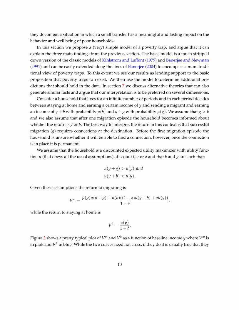
Figure 3 shows a pretty typical plot of Vm and Vh as a function of baseline income y where Vm isin pink and Vh in blue. While the two curves need not cross, if they do it is usually true that they

10

cross only once with Vm being optimal above some threshold income y∗.6 It is much more likelythat the curves will cross like this if the outcome b is sufficiently bad so that u(y + b) is in thevery steep part of the utility function. In the example used to generate Figure 3 this requires thaty + b be close to 0, the point at which the derivative of the ln utility function becomes infinite.

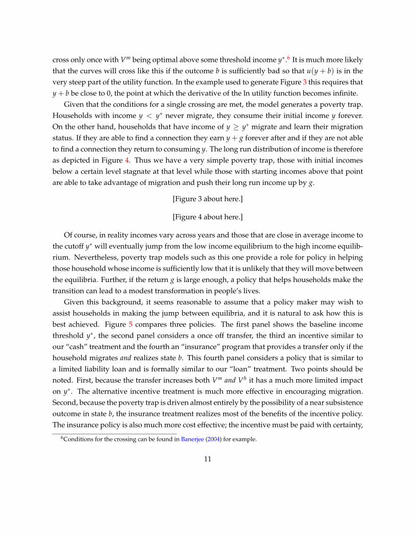
Given that the conditions for a single crossing are met, the model generates a poverty trap.Households with income y < y∗ never migrate, they consume their initial income y forever.On the other hand, households that have income of y ≥ y∗ migrate and learn their migrationstatus. If they are able to find a connection they earn y + g forever after and if they are not ableto find a connection they return to consuming y. The long run distribution of income is thereforeas depicted in Figure 4. Thus we have a very simple poverty trap, those with initial incomesbelow a certain level stagnate at that level while those with starting incomes above that pointare able to take advantage of migration and push their long run income up by g.



Of course, in reality incomes vary across years and those that are close in average income tothe cutoff y∗ will eventually jump from the low income equilibrium to the high income equilib-rium. Nevertheless, poverty trap models such as this one provide a role for policy in helpingthose household whose income is sufficiently low that it is unlikely that they will move betweenthe equilibria. Further, if the return g is large enough, a policy that helps households make thetransition can lead to a modest transformation in people’s lives.

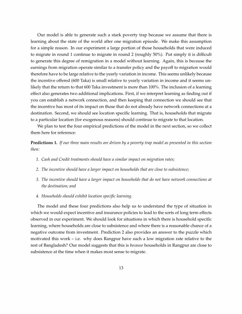
Given this background, it seems reasonable to assume that a policy maker may wish toassist households in making the jump between equilibria, and it is natural to ask how this isbest achieved. Figure 5 compares three policies. The first panel shows the baseline incomethreshold y∗, the second panel considers a once off transfer, the third an incentive similar toour “cash” treatment and the fourth an “insurance” program that provides a transfer only if thehousehold migrates and realizes state b. This fourth panel considers a policy that is similar toa limited liability loan and is formally similar to our “loan” treatment. Two points should benoted. First, because the transfer increases both Vm and Vh it has a much more limited impacton y∗. The alternative incentive treatment is much more effective in encouraging migration.Second, because the poverty trap is driven almost entirely by the possibility of a near subsistenceoutcome in state b, the insurance treatment realizes most of the benefits of the incentive policy.The insurance policy is also much more cost effective; the incentive must be paid with certainty,

6Conditions for the crossing can be found in Banerjee (2004) for example.

11

while the insurance only pays out with probability µ(b). To translate this into our practicalsetting, the loan was repaid in roughly 85% of cases and the total cost of the loan treatment(excluding operating costs) is therefore only 15% of the cost of the incentive treatment.


These two observations translate into two important implications for our experiment. First,we can quantify what it means for the impact of the incentive to be “large”. Given the parame-ters used in Figure 5 the transfer reduces y∗ from 0.275 to 0.259. On the other hand, the incentivedecreases y∗ to 0.241, that is, the same size incentive has roughly twice the impact.7 Anotherway to see this is to note that an incentive of this size has the same impact as an income trans-fer of over twice the size. We, therefore, expect our incentive scheme to have a large impactrelative to yearly income variation that is roughly the same size, and this gives scope for anincentive policy to be cost effective in moving households between equilibria. Second, becausethe insurance policy realizes the lions share of the gain from the incentive policy, we predict thatempirically our “cash” and “loan” treatments will have a similar size impact on the migrationrate.

How general are these results and when would we expect them to hold? The situationconsidered in Figure 5 has a particular feature. Household income y∗ is very low, in that it fallsin the very steep part of the utility function used for the example. This implies that the transferpolicy has a relatively large impact on Vh and therefore that the effect of the incentive is largerelative to the effect of the transfer. If, however, y∗ is high relative to subsistence then this will nolonger be the case. Figure 6 illustrates. The left panel shows how a transfer will affect the curvesVm and Vh, while the right panel illustrates the impact of an incentive. Because income in thisexample is relatively far from the subsistence point (which is 0 given the ln utility function used)the transfer has only a small impact on Vh and as a result the incentive and transfer policies havea similar impact. In such a context it seems unlikely that our incentive would have much of animpact as it is small relative to yearly variation in income and therefore most of the householdsthat are far from subsistence that would be affected by our policy will already have moved tothe high income equilibrium. This reasoning combined with the fact that the overall impact ofour incentive on Vm will be largest when y is small (due to concavity of the utility function)leads us to predict that our treatments will have a larger effect on those households that areclose to subsistence.


7This assumes that households are uniformly distributed with respect to income.

12

Our model is able to generate such a stark poverty trap because we assume that there islearning about the state of the world after one migration episode. We make this assumptionfor a simple reason. In our experiment a large portion of those households that were inducedto migrate in round 1 continue to migrate in round 2 (roughly 50%). Put simply it is difficultto generate this degree of remigration in a model without learning. Again, this is because theearnings from migration operate similar to a transfer policy and the payoff to migration wouldtherefore have to be large relative to the yearly variation in income. This seems unlikely becausethe incentive offered (600 Taka) is small relative to yearly variation in income and it seems un-likely that the return to that 600 Taka investment is more than 100%. The inclusion of a learningeffect also generates two additional implications. First, if we interpret learning as finding out ifyou can establish a network connection, and then keeping that connection we should see thatthe incentive has most of its impact on those that do not already have network connections at adestination. Second, we should see location specific learning. That is, households that migrateto a particular location (for exogenous reasons) should continue to migrate to that location.

We plan to test the four empirical predictions of the model in the next section, so we collectthem here for reference:

Predictions 1. If our three main results are driven by a poverty trap model as presented in this sectionthen:

1. Cash and Credit treatments should have a similar impact on migration rates;

2. The incentive should have a larger impact on households that are close to subsistence;

3. The incentive should have a larger impact on households that do not have network connections atthe destination; and

4. Households should exhibit location specific learning.

The model and these four predictions also help us to understand the type of situation inwhich we would expect incentive and insurance policies to lead to the sorts of long term effectsobserved in our experiment. We should look for situations in which there is household specificlearning, where households are close to subsistence and where there is a reasonable chance of anegative outcome from investment. Prediction 2 also provides an answer to the puzzle whichmotivated this work – i.e. why does Rangpur have such a low migration rate relative to therest of Bangladesh? Our model suggests that this is because households in Rangpur are close tosubsistence at the time when it makes most sense to migrate.

13

6 Additional Tests of the Model

In this section we provide evidence that is consistent with the for predictions from our model.The first prediction of our model has already been verified. The migration rate in the cash

treatment is 58.96% while in the credit treatment it is 56.8% and the difference is not statisticallysignificant. This is consistent with the claim that the cash and credit treatments should havesimilar impacts on the migration rate, with the credit treatment being slightly less effective.

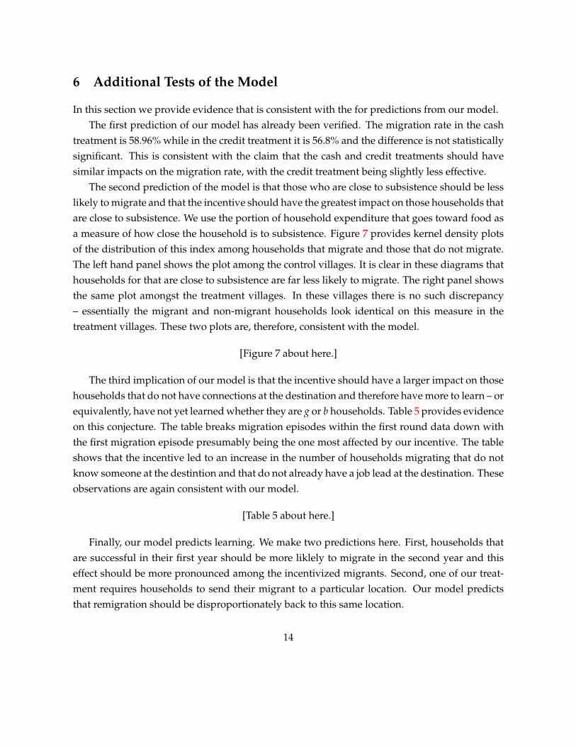
The second prediction of the model is that those who are close to subsistence should be lesslikely to migrate and that the incentive should have the greatest impact on those households thatare close to subsistence. We use the portion of household expenditure that goes toward food asa measure of how close the household is to subsistence. Figure 7 provides kernel density plotsof the distribution of this index among households that migrate and those that do not migrate.The left hand panel shows the plot among the control villages. It is clear in these diagrams thathouseholds for that are close to subsistence are far less likely to migrate. The right panel showsthe same plot amongst the treatment villages. In these villages there is no such discrepancy– essentially the migrant and non-migrant households look identical on this measure in thetreatment villages. These two plots are, therefore, consistent with the model.


The third implication of our model is that the incentive should have a larger impact on thosehouseholds that do not have connections at the destination and therefore have more to learn – orequivalently, have not yet learned whether they are g or b households. Table 5 provides evidenceon this conjecture. The table breaks migration episodes within the first round data down withthe first migration episode presumably being the one most affected by our incentive. The tableshows that the incentive led to an increase in the number of households migrating that do notknow someone at the destintion and that do not already have a job lead at the destination. Theseobservations are again consistent with our model.


Finally, our model predicts learning. We make two predictions here. First, households thatare successful in their first year should be more liklely to migrate in the second year and thiseffect should be more pronounced among the incentivized migrants. Second, one of our treat-ment requires households to send their migrant to a particular location. Our model predictsthat remigration should be disproportionately back to this same location.

14

Table 6 provides evidence in favor of the first question. Among the incentivized villages,households that remigrate are those that were successful in the first round – i.e. those that havehigher savings and earnings in the first round. In contrast there is a much weaker different inthe impact of success among non-treatment villages. This is consistent with the model and theidea that the treatment households have something to learn, while the non-treatment villagesdo not.


Table 7 provides evidence on the second conjecture. It shows results of a multinomial logitand confirms that households that were successful in a particular location were likely to returnto that location.


7 Alternatives

In this section we discuss alternative explanations for our empirical results. The most plausiblealternative explanation is that, during the lean season, households face a strong liquidity con-straint – they simply do not have the 600 Taka required to pay for a bus ticket and thereforecannot migrate. Relieving the liquidity constraint in one year could lead to ongoing migrationeither through learning as discussed above or because increased income relaxes the liquidityconstraint again the following year.8 Such an explanation can account for the majority of ourfacts. A large portion of the population may be liquidity constrained in any given year leadingto the large effect of the incentive, the return to migration can be positive and yet people do notmigrate because they lack can, the impact of cash and credit treatments will be the same and,to the extent that subsistence is correlated with the liquidity constraint, we would expect theincentive to have a greater impact on those close to subsistence.

Nevertheless we do not thing a liquidity constraint can explain our results. Given the strongrepeat impact on the second year, and the small size of the transfer, a liquidity constraint storywould not hold over time. That is, we would expect all households to have received a suffi-ciently strong positive income shock in the past to have overcome the liquidity constraint andmoved to the rich equilibrium prior to our intervention. For example, year on year average ab-solute deviation in weekly expenditure in our sample is 307 Taka between rounds one and two

8It should be noted that some form of credit constraint is required for the poverty trap model above to work. Theliquidity constraint discussed here is a more severe form of credit constraint.

15

and 368 Taka between rounds two and three. The standard deviation of absolute deviation inconsumption is 635 and 508 Taka respectively. While part of this is no doubt driven by mea-surement error, these figures show what seems obvious, season on season variation in incomeslikely swamps the 600 Taka of our incentive. This criticism applies to all mechanisms that treatthe incentive as a one time transfer. Further to this basic criticism, the lean season in this regionlasts for around 3 months. It is hard to see how any household that has sufficient funds, eitheras storage or recurring wages, to survive this period would be unable to find 600 Taka. Thismay be a very costly choice, but it will be possible. Liquidity constraints therefore seem to becounter factual.

The above discussion applies equally to any mechanism that does not emphasize the incen-tive effect of our treatments. This observation, however, raises a perhaps troubling point forour preferred model. The basic argument against 600 Taka having a large effect in the form of atransfer is that yearly variation in income is larger. Therefore, for our incentive to work it mustbe the case that many households would prefer to keep a once of transfer of 600 Taka rather thanspend it one migration. But this implies that the welfare impact of our intervention is boundedabove by the benefit of giving each household 600 Taka to use as they please and the householdsnot migrating. This point is of course obvious in a fully rational model because households al-ways prefer to have money without constraints. We leave it to the reader to determine whetherthey believe that it is reasonable to assume this. Alternative models that posit less rationality,either in the form of excessive impatience (δ low), non-rational expectations (µ(b) too low) orsome reason why the household is consistently on the poverty line despite variation in income(for example hyperbolic disounting a la Laibson (1997) and Duflo et al. (2009)) can make someroom for policy makers to believe that the welfare gains of this intervention are larger than thepurely rational model would imply.

8 Conclusions

We conducted a randomized experiment in which we incentivized households in Rangpur tosend a seasonal migrant to an urban area. The main results show that a small incentive led to alarge increase in the number of seasonal migrants, that the migration was successful in the sensethat it led to an average increase in consumption of around 35% and that households given theincentive in one year continued to be more likely to migrate in the following year.

We argue that the results are consistent with a simple (rational) model of a poverty trapwhere households that are close to subsistence are unable to learn whether migration is suc-

16

cessful due to a small possibility that migrating will turn out badly, leaving households con-sumption below subsistence.

From a policy perspective, the results support a policy of providing micro-insurance thatmitigates the potential downside of experimentation. Our analysis also suggests that such apolicy will be particularly beneficial where households are close to subsistence, risk averse andcould benefit from a technology that requires individual level experimentation in order to de-termine profitability.


References

Banerjee, A., “The Two Poverties,” in Stefan Dercon, ed., Insurance against poverty, Oxford Schol-arship Online Monographs, 2004, pp. 59–76.

Banerjee, A.V. and A.F. Newman, “Risk-bearing and the theory of income distribution,” TheReview of Economic Studies, 1991, 58 (2), 211.

Duflo, E., M. Kremer, and J. Robinson, “Nudging farmers to use fertilizer: theory and experi-mental evidence from Kenya,” NBER Working Paper, 2009.

Foster, A.D. and M.R. Rosenzweig, “Microeconomics of technology adoption,” Annu. Rev.Econ., 2010, 2 (1), 395–424.

Kihlstrom, R.E. and J.J. Laffont, “A general equilibrium entrepreneurial theory of firm forma-tion based on risk aversion,” The Journal of Political Economy, 1979, 87 (4), 719–748.

Laibson, David, “Golden Eggs and Hyperbolic Discounting,” Quarterly Journal of Economics, 4771997, 113 (2), 443.

17

List of Figures

1 Seasonality of Rice Prices . . . . . . . . . . . . . . . . . . . . . . . . . . . . . . . . . 192 Seasonality of Food Expenditure . . . . . . . . . . . . . . . . . . . . . . . . . . . . 203 The return to migration as a function of income . . . . . . . . . . . . . . . . . . . . 214 Long run income distribution . . . . . . . . . . . . . . . . . . . . . . . . . . . . . . 225 The effect of policy on cutoff for migration . . . . . . . . . . . . . . . . . . . . . . 236 The effect of policy on cutoff for migration with income above subsistence . . . . 247 Kernel Density Plots of Subsistence Index by Treatment Status . . . . . . . . . . . 25

18

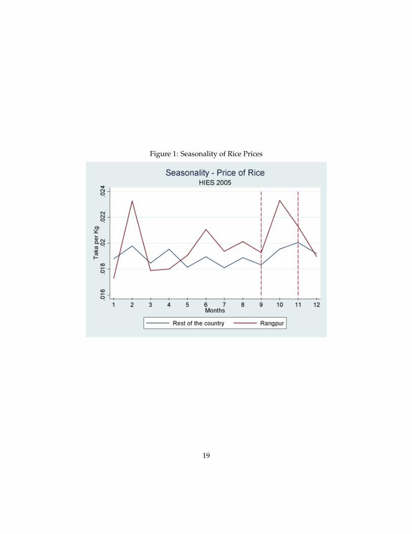
Figure 1: Seasonality of Rice Prices

19

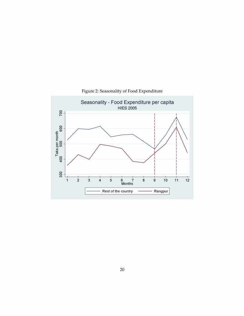
Figure 2: Seasonality of Food Expenditure

20

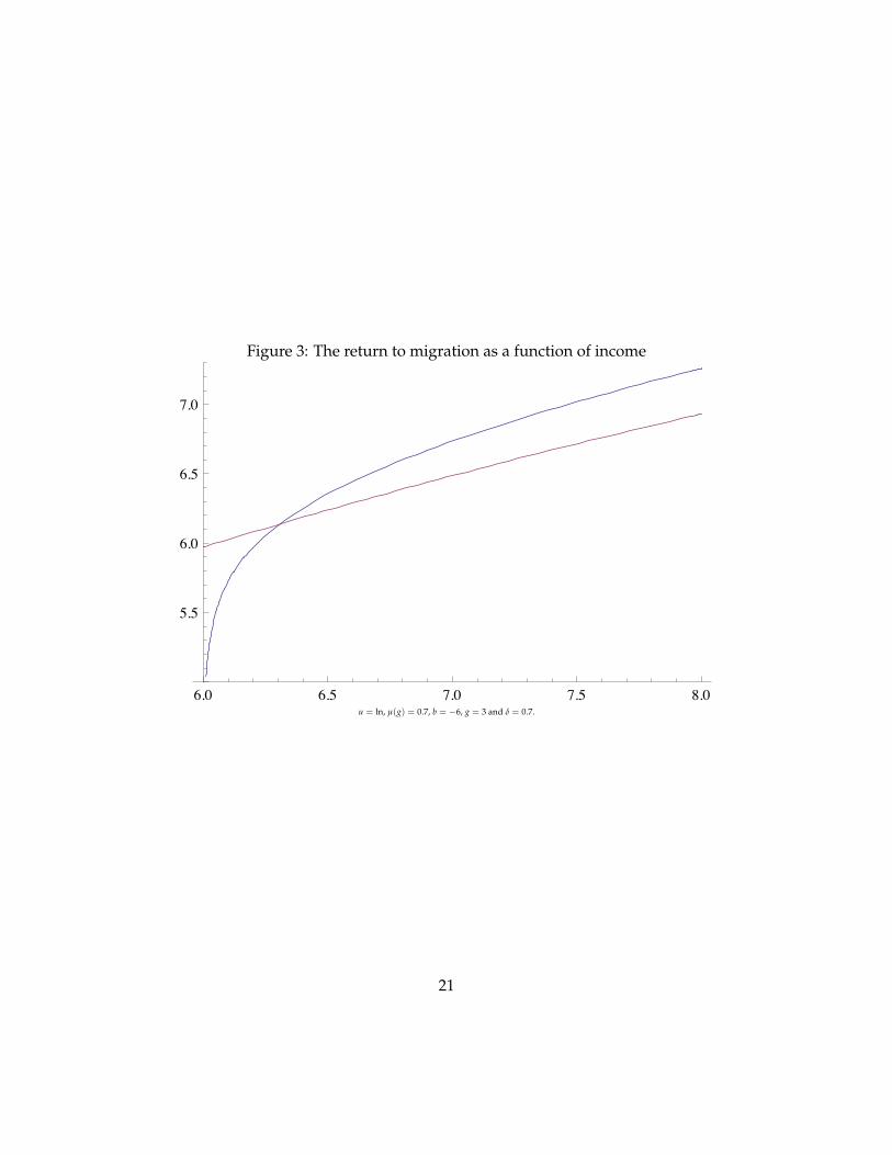
Figure 3: The return to migration as a function of income

6.0 6.5 7.0 7.5 8.0

5.5

6.0

6.5

7.0

u = ln, µ(g) = 0.7, b = −6, g = 3 and δ = 0.7.

21

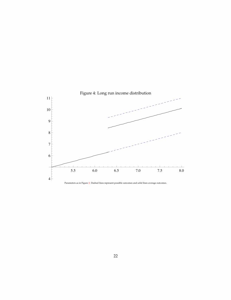
Figure 4: Long run income distribution

5.5 6.0 6.5 7.0 7.5 8.0

4

6

7

8

9

10

11

Parameters as in Figure 3. Dashed lines represent possible outcomes and solid lines average outcomes.

22

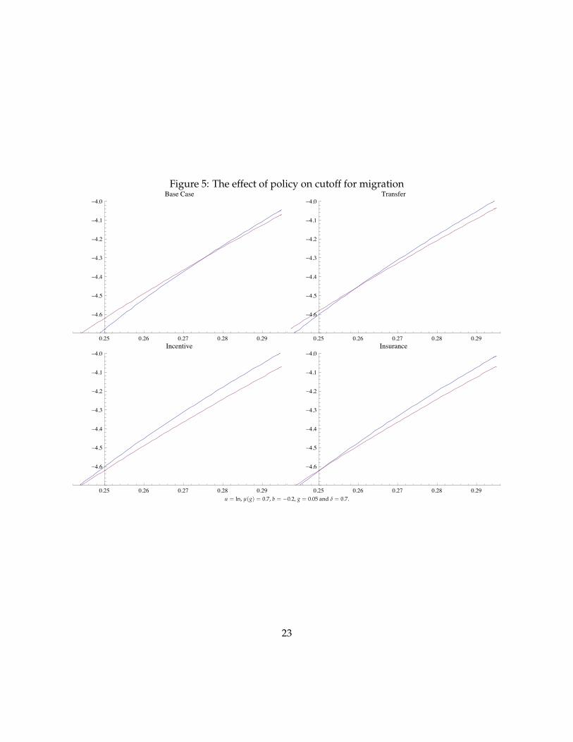
Figure 5: The effect of policy on cutoff for migration

0.25 0.26 0.27 0.28 0.29

�4.6

�4.5

�4.4

�4.3

�4.2

�4.1

�4.0Base Case

0.25 0.26 0.27 0.28 0.29

�4.6

�4.5

�4.4

�4.3

�4.2

�4.1

�4.0Transfer

0.25 0.26 0.27 0.28 0.29

�4.6

�4.5

�4.4

�4.3

�4.2

�4.1

�4.0Incentive

0.25 0.26 0.27 0.28 0.29

�4.6

�4.5

�4.4

�4.3

�4.2

�4.1

�4.0Insurance

u = ln, µ(g) = 0.7, b = −0.2, g = 0.05 and δ = 0.7.

23

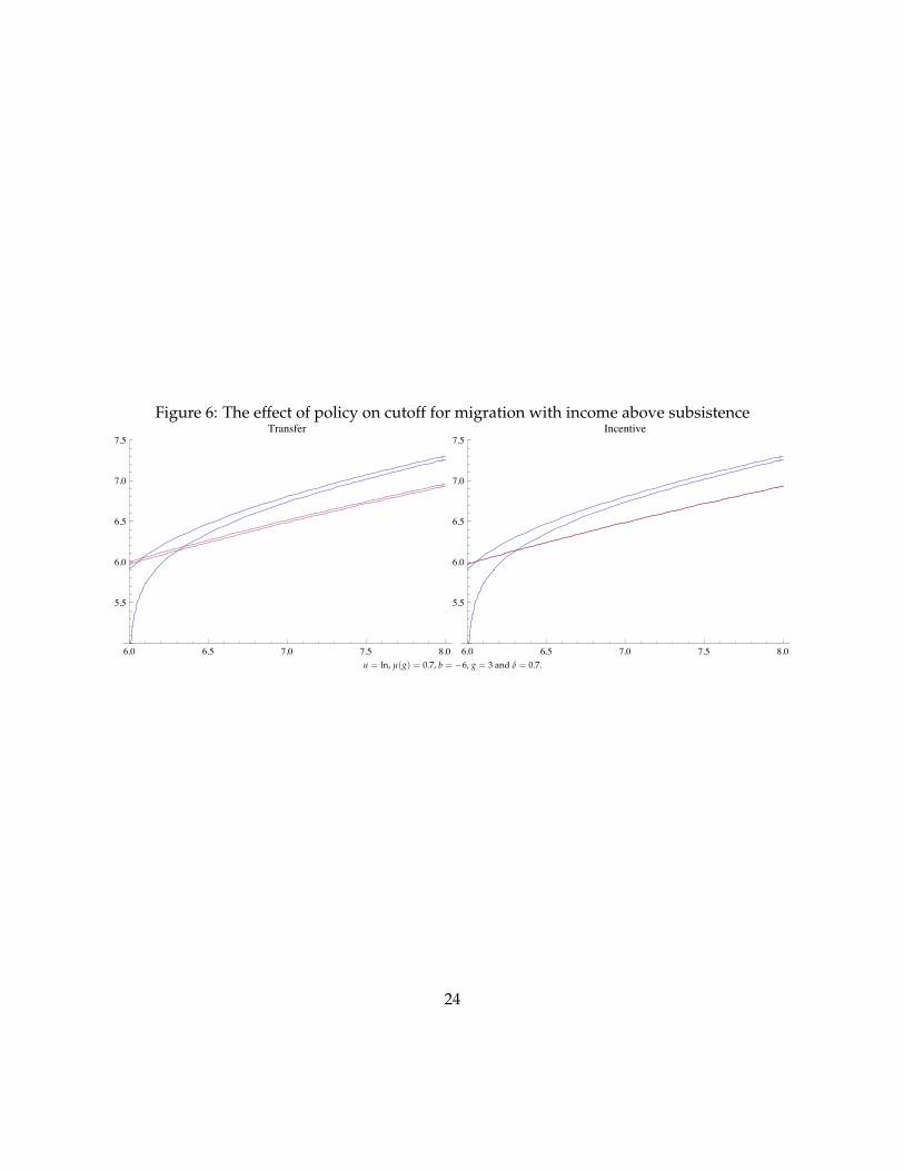
Figure 6: The effect of policy on cutoff for migration with income above subsistence

6.0 6.5 7.0 7.5 8.0

5.5

6.0

6.5

7.0

7.5Transfer

6.0 6.5 7.0 7.5 8.0

5.5

6.0

6.5

7.0

7.5Incentive

u = ln, µ(g) = 0.7, b = −6, g = 3 and δ = 0.7.

24

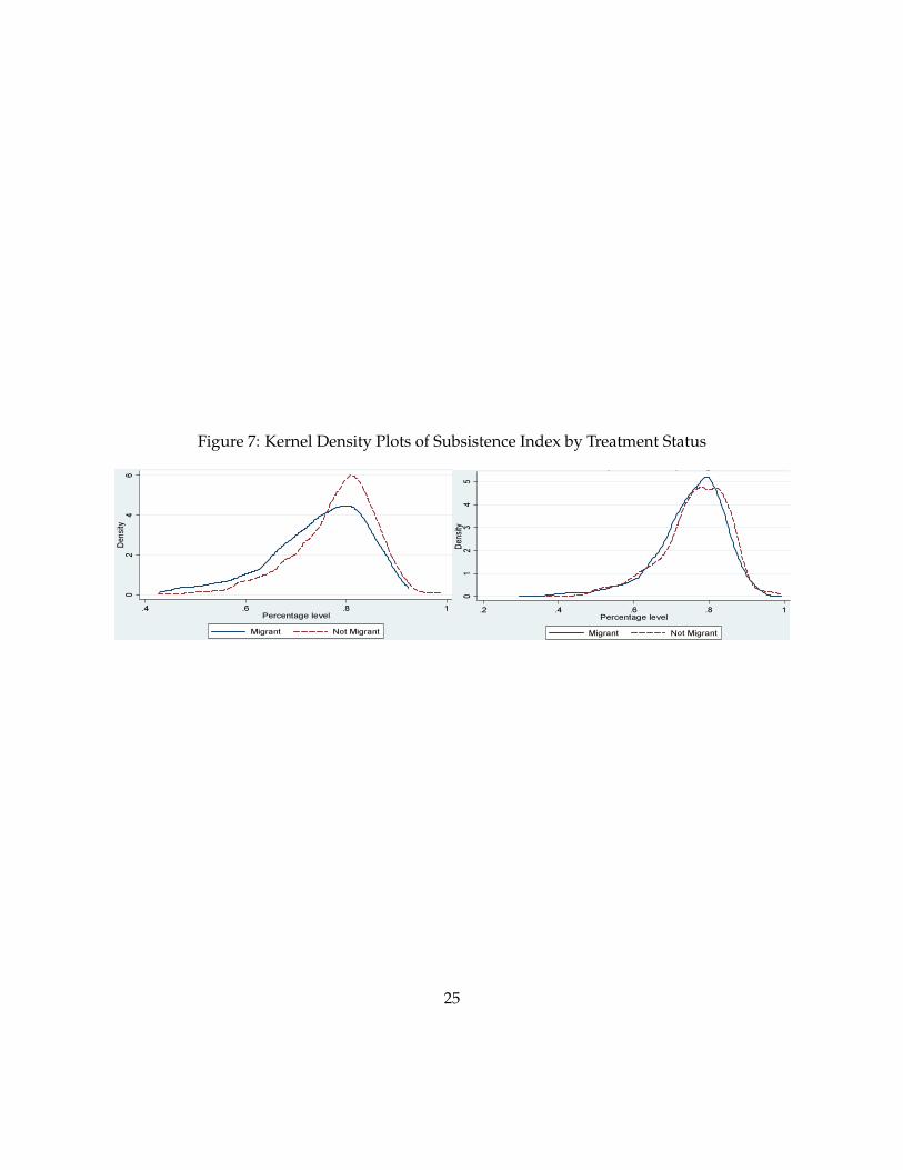
Figure 7: Kernel Density Plots of Subsistence Index by Treatment Status

25

List of Tables

1 Program Takeup . . . . . . . . . . . . . . . . . . . . . . . . . . . . . . . . . . . . . . 272 Effects of Migration on Expenditure Amongst Remaining Household Members . 283 Earnings & Saving from Migration (Round 2) . . . . . . . . . . . . . . . . . . . . . 294 Earnings for non-migrants . . . . . . . . . . . . . . . . . . . . . . . . . . . . . . . . 305 Who Migrates by Treatment Group . . . . . . . . . . . . . . . . . . . . . . . . . . . 316 Remigration by Earnings in First Migration Episode . . . . . . . . . . . . . . . . . 327 Remigration by Earnings in First Migration Episode . . . . . . . . . . . . . . . . . 338 Structure of the Randomization . . . . . . . . . . . . . . . . . . . . . . . . . . . . . 34

26

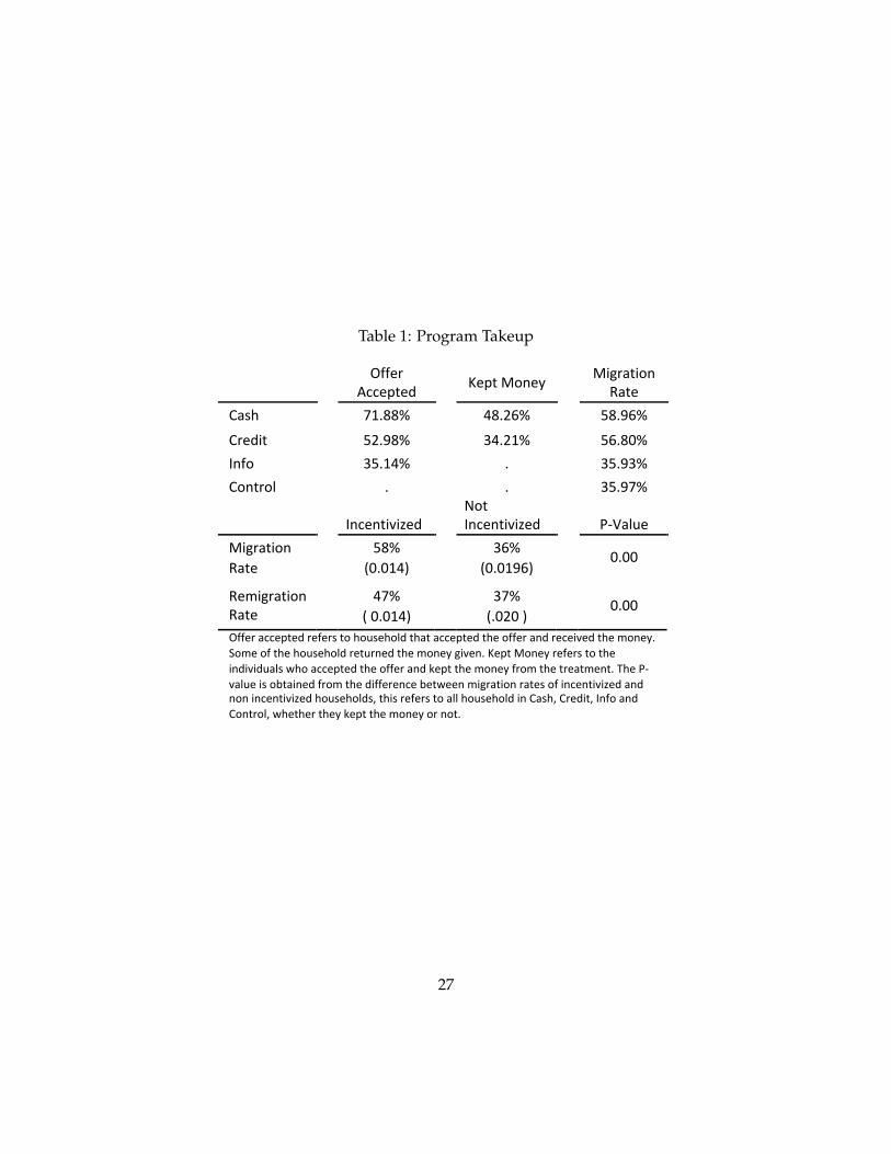
Table 1: Program Takeup!"#$%&'(&)*+,*"-&!".%/01&"23&45,*"65+2&7"6%8&

&& &9::%*&

;<<%16%3&& =%16&4+2%>& &

45,*"65+2&7"6%&

?"8@& ! A'BCCD& & ECBFGD& & HCBIGD&

?*%356& ! HFBICD& & JEBF'D& & HGBCKD&

L2:+& ! JHB'ED& & B& & JHBIJD&

?+26*+$& ! B& & B& & JHBIAD&

&& & L2<%265M5N%3& &O+6&L2<%265M5N%3& & )/P"$0%&

! HCD& & JGD& &45,*"65+2&7"6%& ! QKBK'ER& & QKBK'IGR& &

KBKK&

! EAD& & JAD& &7%-5,*"65+2&7"6%& !! Q&KBK'ER& && QBKFK&R& &&

KBKK&

9::%*&"<<%16%3&*%:%*8&6+&@+08%@+$3&6@"6&"<<%16%3&6@%&+::%*&"23&*%<%5M%3&6@%&-+2%>B&S+-%&+:&6@%&@+08%@+$3&*%60*2%3&6@%&-+2%>&,5M%2B&=%16&4+2%>&*%:%*8&6+&6@%&5235M530"$8&T@+&"<<%16%3&6@%&+::%*&"23&.%16&6@%&-+2%>&:*+-&6@%&6*%"6-%26B&!@%&)/M"$0%&58&+#6"52%3&:*+-&6@%&35::%*%2<%&#%6T%%2&-5,*"65+2&*"6%8&+:&52<%265M5N%3&"23&2+2&52<%265M5N%3&@+08%@+$38U&6@58&*%:%*8&6+&"$$&@+08%@+$3&52&?"8@U&?*%356U&L2:+&"23&?+26*+$U&T@%6@%*&6@%>&.%16&6@%&-+2%>&+*&2+6B&

!

27

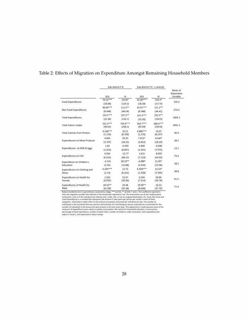
Table 2: Effects of Migration on Expenditure Amongst Remaining Household Members

! ! ! ! ! ! ! ! ! ! !! "#$%&'()*'+)!,-.-! ! "#$%&'()*'+)!,-.-!/!+01)*02(! ! !

!!

34"! !! 56! ! 34"! ! 56! !

7891!0:!;8<81&81)!69*'9$28!

! =>-?@AAA! ! BBC-DA! ! >B-CEAAA! ! BBE-FA! !,00&!.G<81&')#*8(!!

! H?D-EDI! ! H?BC-BI! ! H?D-BDI! ! H??=->I! !=B>-B!

! C@-ECAAA! ! ???-JAA! ! JJ->?AAA! ! ???-BAA! !K01!,00&!.G<81&')#*8(!

! HD-CCDI! ! HC>-JCI! ! HD-FDDI! ! HCC-C?I! !B=C-C!

! ?BC-JAAA! ! FF=-JAA! ! ?C=-CAAA! ! FFB-JAA! !L0)92!.G<81&')#*8(!

! HBB-F@I! ! H?JC-?I! ! HBB-B@I! ! H?CF-EI! !?EEF-?!

! BF?-FAAA! ! =B>-CAAA! ! B@B-=AAA! ! @@@-@AAA! !L0)92!M920*'+!'1)9N8!

! HCE-@?I! ! HBFD-?I! ! HCB-@>I! ! HBFC-DI! !BE>?-F!

! C-?@DAAA! ! ?E-J?! ! C-DD>AAA! ! ?E-E=! !L0)92!M920*'8(!:*0O!P*0)8'1!

! H?-?=@I! ! HD-=E>I! ! H?-B=@I! ! HD-BF=I! !C@->!

! C-@EJ! ! B>-BJ! ! =-E?FA! ! FF-@EA! !.G<81&')#*8(!01!789)!P*0&#+)(!

! HF-=E=I! ! H?D-?JI! ! HF-DJBI! ! H?D-B>I! !BD-B!

! ?-@C! ! %E-J>J! ! E->E>! ! %E->FD! !.G<81&')#*8(!!01!7'2N!Q!.RR(!

! H?-CJFI! ! HD-E@=I! ! H?-CF?I! ! H=->=JI! !?F-?!

! E-J@C! ! %?B-==! ! ?-@?J! ! %D-@>F! !.G<81&')#*8(!01!,'(S!

! H@-JJBI! ! HCD-?BI! ! H=-?FFI! ! HCF-EFI! !=C-C!

! %F-B?@! ! BD-?EAA! ! %C-ED>A! ! B?-EJA! !.G<81&')#*8!01!MS'2&*81T(!.&#+9)'01! ! HB-FCI! ! H?B-DDI! ! HB-CFCI! ! H?B-E@I! !

?D-B!

! @-BCFAAA! ! ?B-=B! ! @->BDAAA! ! ?B-JCA! !.G<81&')#*8(!01!M20)S'1R!91&!"S08(! ! H?-JFI! ! HD-?E?I! ! H?-JBDI! ! H=-F>JI! !

FD-D!

! ?-J@J! ! JF-F=! ! E-BEC! ! JE-DE! !.G<81&')#*8(!01!U892)S!:0*!,8O928! ! H@->FJI! ! HF>-F@I! ! H=-F?CI! ! HF>-=DI! !

@?-J!

! ?D-FBAA! ! BC-CD! ! ?>-E>AA! ! ?@-CB! !.G<81&')#*8(!0:!U892)S!:0*!7928! ! HD-?>>I! ! HFJ-BDI! ! HD-@CEI! ! HF=-=EI! !

=?-C!

V0$#()!()91&9*&!8**0*(!'1!<9*81)S8(8(W!+2#()8*8&!$X!Y'229R8-!AAA!<ZE-E?W!AA!<ZE-EJW!A!<ZE-?-!LS8!+08::'+'81)!*8<0*)8&!'(!:*0O!)S8!O'R*9)'01!Y9*'9$28!)S9)!'1&'+9)8(!':!)S8!S0#(8S02&(!O'R*9)8&!0*!10)-!LS8!51()*#O81)(!9*8!922!)S8!*91&0O'[9)'01!)*89)O81)(W!(#+S!9(!':!)S8!'1&'Y'&#92!\9(!0::8*8&!+9(SW!+*8&')W!'1:0W!0*!S9(!91!9(('R18&!&8()'19)'01W!8)+-!,00&W!K01!,00&!91&!L0)92!.G<81&')#*8(!'(!9!Y9*'9$28!)S9)!*8<*8(81)(!)S8!9O0#1)!'1!)9N9!(<81)!<8*!<8*(01!<8*!O01)S!'1!89+S!0:!)S8(8!+9)8R0*'8(-!L0)92!M920*'+!'1)9N8!*8:8*(!)0!)S8!9O0#1)!0:!]#91)')X!+01(#O8&!<8*!'1&'Y'&#92!<8*!&9X-!LS8!1#O$8*!0:!'1&'Y'&#92(!'1!)S8!S0#(8S02&!)S9)!\8!#(8&!9(!9!&810O'19)0*!:0*!+92+#29)'1R!<8*!<8*(01!8G<81&')#*8(!'(!8()'O9)8&!:0*!)S8!1#O$8*!0:!'1&'Y'&#92(!'1!)S8!S0#(8!)S9)!\8*8!<*8(81)!'1!)S8!29()!(8Y81!&9X(-!LS'(!9&^#()O81)!'(!O9&8!$8+9#(8!(0O8!0:!)S8!O89(#*8(!0:!8G<81&')#*8(!\8*8!9(N8&!9(!\88N2X!+01(#O<)'01-!_8!+01)*02!:0*!S0#(8S02&!8&#+9)'01W!'1+0O8!<*0GXW!<8*+81)9R8!0:!:00&!8G<81&')#*8W!1#O$8*!0:!9&#2)!O928(W!1#O$8*!0:!+S'2&*81W!+*8&')!+01()*9'1)(W!)0)92!8G<81&')#*8!<8*!+9<')9!'1!*0#1&!?W!91&!8G<8+)9)'01(!9$0#)!O01R9-!!

!

!!

28

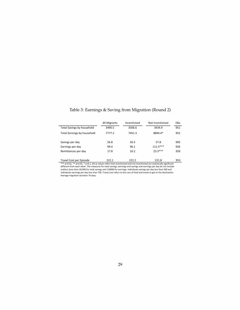
Table 3: Earnings & Saving from Migration (Round 2)

! ! ! ! ! ! ! ! !!! ! "##!$%&'()*+! ! ,)-.)*%/%0.1! ! 23*!,)-.)*%/%0.1! ! 45+!

63*(#!7(/%)&+!58!93:+.93#1!! ! ;<=>?@! ! ;@>A?A! ! ;<;<?=! ! =@B!

63*(#!C(')%)&+!58!93:+.93#1!! ! DDDD?E! ! D<@B?;! ! FF=<?<G! ! =@E!

! ! ! ! ! ! ! ! !7(/%)&+!H.'!1(8!! ! @A?F! ! @A?@! ! @D?F! ! =>@!

C(')%)&+!H.'!1(8!! ! ==?<! ! =A?B! ! BBB?@GGG! ! =EA!

I.J%**()-.+!H.'!1(8!! ! BD?F! ! BA?E! ! E;?;GGG! ! =EA!

! ! ! ! ! ! ! ! !

6'(/.#!K3+*!H.'!CH%+31.! ! EEE?B! ! EEE?E! ! EEB?F! ! =@;!GGG!HL>?>BM!GG!HL>?>@M!G!HL>?BM!*9.!HN/(#:.+!'.O.'+!*9(*!%)-.)*%/%0.1!()1!)3*!%)-.)*%/%0.1!('.!+*(*%+*%-(##8!+%&)%O%-()*!1%OO.'.)*!O'3J!.(-9!3*9.'?!69.!J.(+:'.+!O3'!*3*(#!+(/%)&+M!.(')%)&+!()1!+(/%)&+!()1!.(')%)&+!H.'!1(8!13!)3*!%)-#:1.!3:*#%.'+!PQ.++!*9()!E>M>>>!O3'!*3*(#!+(/%)&+!()1!BE>>>>!O3'!.(')%)&+?!,)1%/%1:(#+!+(/%)&+!H.'!1(8!#.++!*9()!@>>!()1!%)1%/%1:(#+!.(')%)&+!H.'!1(8!#.++!*9()!D>>?!6'(/.#!-3+*!'.O.'+!*3!*9.!-3+*!3O!O331!()1!*'(/.#!*3!&.*!*3!*9.!1.+*%)(*%3)?!"/.'(&.!J%&'(*%3)!1:'(*%3)!DA!1(8+?!

!

29

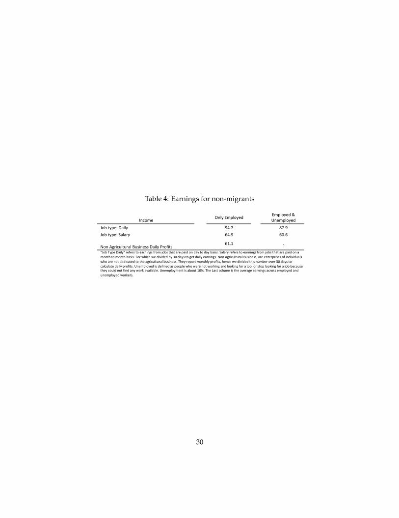
Table 4: Earnings for non-migrants

!"#$%&'' (")*'+%,)$*&-'' '

+%,)$*&-'.'/"&%,)$*&-'

0$1'2*,&3'456)*' ' 789:' ' ;:97'

0$1'2*,&3'<5)5=*' ' >897' ' >?9>'

@$"'AB=6#C)2C=5)'DCE6"&EE'456)*'F=$G62E' '>H9H'

'9'

I0$1'J*,&'456)*I'=&G&=E'2$'&5="6"BE'G=$%'K$1E'2L52'5=&',56-'$"'-5*'2$'-5*'15E6E9'<5)5=*'=&G&=E'2$'&5="6"BE'G=$%'K$1E'2L52'5=&',56-'$"'5'%$"2L'2$'%$"2L'15E6E9'M$='NL6#L'N&'-6O6-&-'1*'P?'-5*E'2$'B&2'-56)*'&5="6"BE9'@$"'AB=6#C)2C=5)'DCE6"&EEQ'5=&'&"2&=,=6E&E'$G'6"-6O6-C5)E'NL$'5=&'"$2'-&-6#52&-'2$'2L&'5B=6#C)2C=5)'1CE6"&EE9'JL&*'=&,$=2'%$"2L)*',=$G62EQ'L&"#&'N&'-6O6-&-'2L6E'"C%1&='$O&='P?'-5*E'2$'#5)#C)52&'-56)*',=$G62E9'/"&%,)$*&-'6E'-&G6"&-'5E',&$,)&'NL$'N&=&'"$2'N$=R6"B'5"-')$$R6"B'G$='5'K$1Q'$='E2$,')$$R6"B'G$='5'K$1'1&#5CE&'2L&*'#$C)-'"$2'G6"-'5"*'N$=R'5O56)51)&9'/"&%,)$*%&"2'6E'51$C2'H?S9'JL&'T5E2'#$)C%"'6E'2L&'5O&=5B&'&5="6"BE'5#=$EE'&%,)$*&-'5"-'C"&%,)$*&-'N$=R&=E9''

!

30

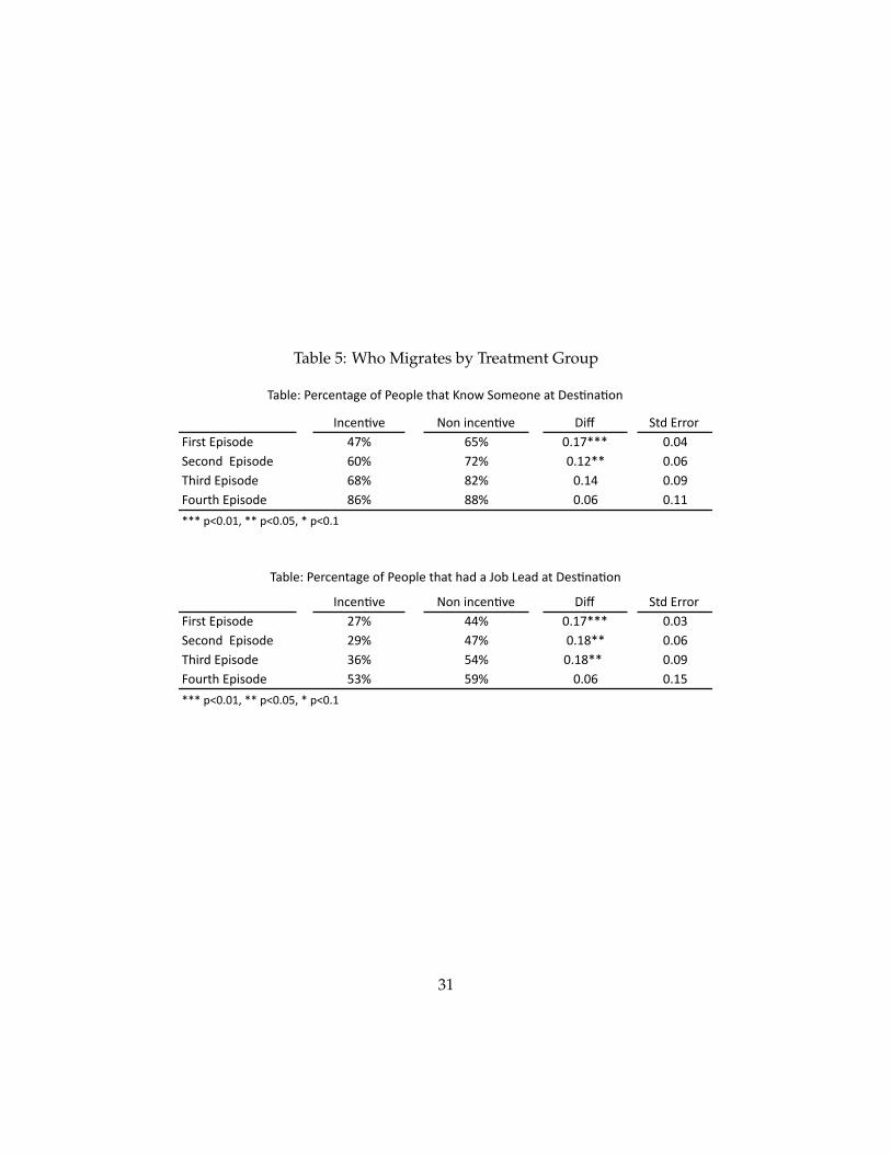
Table 5: Who Migrates by Treatment Group

!"#$"%&$ '(")*"#$"%&$ +*, -./)011(1

2*13.)04*3(/$) 567 897 :;<6=== :;:5

-$#("/))04*3(/$) 8:7 6>7 :;<>== :;:8

?@*1/)04*3(/$) 8A7 A>7 :;<5 :;:B

2(C1.@)04*3(/$) A87 AA7 :;:8 :;<<

!"#$"%&$ '(")*"#$"%&$ +*, -./)011(1

2*13.)04*3(/$) >67 557 :;<6=== :;:D

-$#("/))04*3(/$) >B7 567 :;<A== :;:8

?@*1/)04*3(/$) D87 957 :;<A==) :;:B

2(C1.@)04*3(/$) 9D7 9B7 :;:8 :;<9

?EFG$H)I$1#$".EJ$)(K)I$(4G$).@E.)L"(M)-(N$("$)E.)+$3%"E%("

===)4O:;:<P)==)4O:;:9P)=)4O:;<

?EFG$H)I$1#$".EJ$)(K)I$(4G$).@E.)@E/)E)Q(F)R$E/)E.)+$3%"E%("

===)4O:;:<P)==)4O:;:9P)=)4O:;<

31

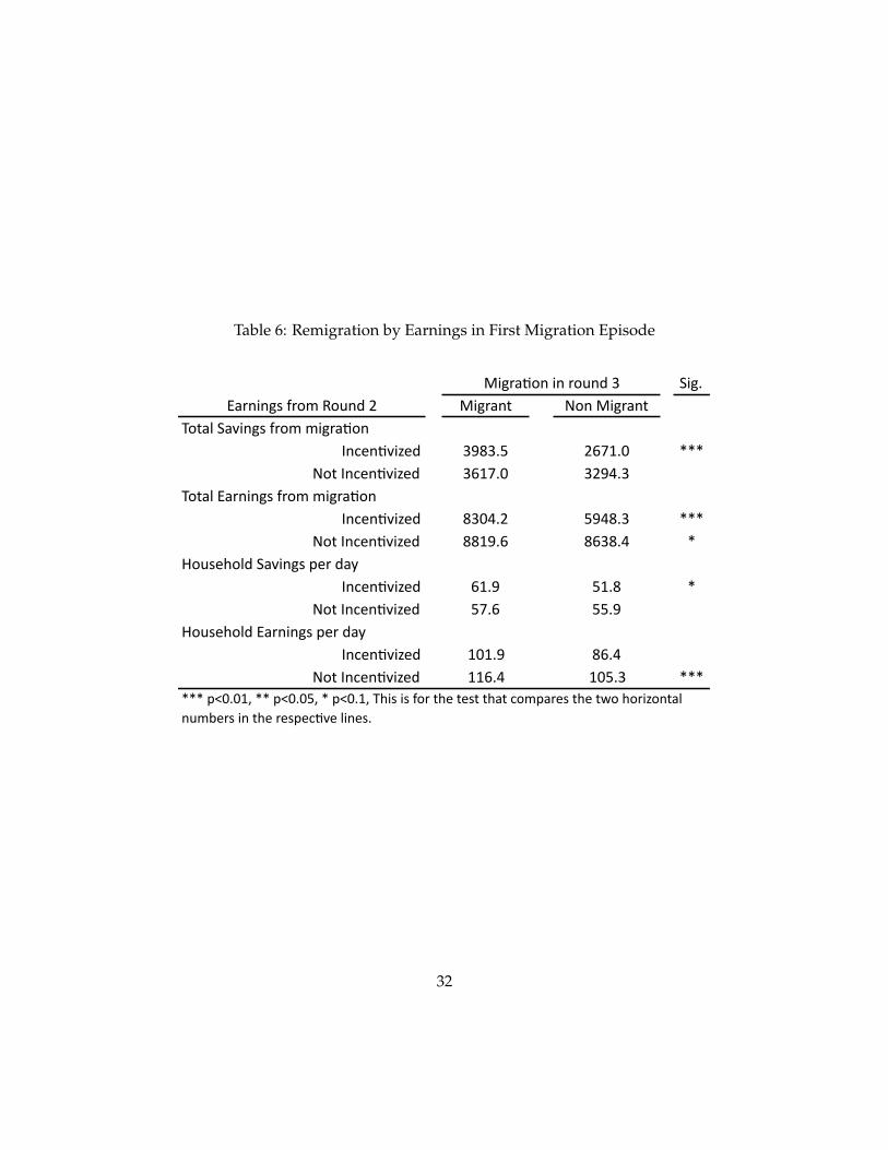
Table 6: Remigration by Earnings in First Migration Episode

!"#$%"#&'() *+(,%"#&'()

-+)'.,!'/"(#0,1&+2,2"#&'3+(,4(56(3/"768 9:;9$< =>?@$A BBB

*+),4(56(3/"768 9>@?$A 9=:C$9-+)'.,D'&("(#0,1&+2,2"#&'3+(,

4(56(3/"768 ;9AC$= <:C;$9 BBB*+),4(56(3/"768 ;;@:$> ;>9;$C B

E+F06G+.8,!'/"(#0,H6&,8'I,4(56(3/"768 >@$: <@$; B

*+),4(56(3/"768 <?$> <<$:E+F06G+.8,D'&("(#0,H6&,8'I,

4(56(3/"768 @A@$: ;>$C*+),4(56(3/"768 @@>$C @A<$9 BBB

%"#&'3+(,"(,&+F(8,9

BBB,HJA$A@K,BB,HJA$A<K,B,HJA$@K,-G"0,"0,1+&,)G6,)60),)G'),5+2H'&60,)G6,)L+,G+&"7+()'.,(F2M6&0,"(,)G6,&60H653/6,."(60$

-'M.6N,D'&("(#0,MI,O62"#&'3+(

D'&("(#0,1&+2,O+F(8,=

32

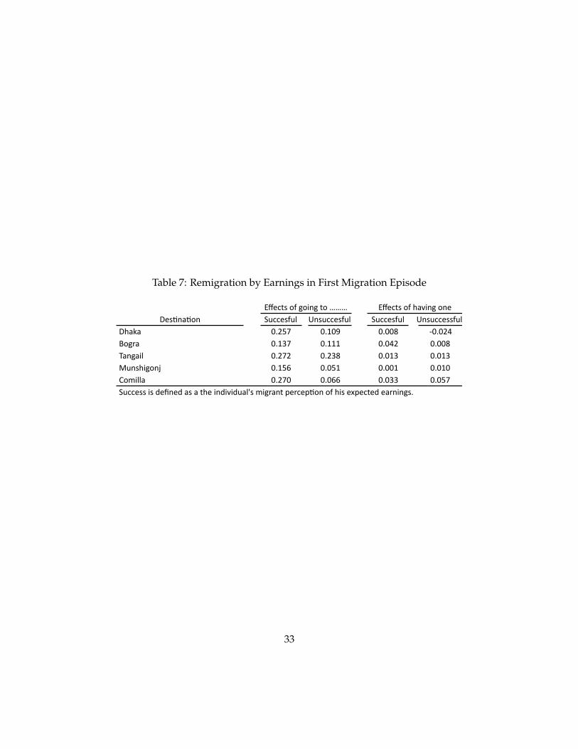
Table 7: Remigration by Earnings in First Migration Episode

!"##$%&"' ()%"##$%&"' !"##$%&"' ()%"##$%%&"'*

+,-.- /0123 /04/5 /0//6 7/0/18

9:;<- /04=3 /0444 /0/81 /0//6

>-);-?' /0131 /01=6 /0/4= /0/4=

@")%,?;:)A /042B /0/24 /0//4 /0/4/

C:D?''- /013/ /0/BB /0/== /0/23

!"##$%%*?%*E$F)$E*-%*-*G,$*?)E?H?E"-'I%*D?;<-)G*J$<#$JK:)*:&*,?%*$LJ$#G$E*$-<)?);%0

MN$#G%*:&*;:?);*G:*OOO MN$#G%*:&*,-H?);*:)$*

+$%K)-K:)

33

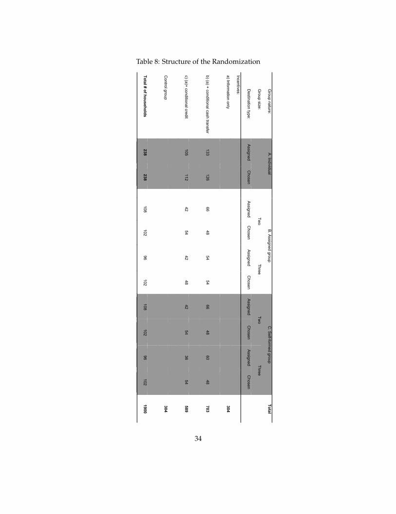
Table 8: Structure of the Randomization

Group nature:

A. Individual

B

. Assigned group

C. S

elf-formed group

Total

Group size:

Tw

o Three

Two

Three

Destination type:

Assigned

Chosen

A

ssigned C

hosen A

ssigned C

hosen A

ssigned C

hosen A

ssigned C

hosen

Incentives:

a) Information only

304

b) (a) + conditional cash transfer 133

126

66 48

54 54

66 48

60 48

703

c) (a)+ conditional credit 105

112

42 54

42 48

42 54

36 54

589

Control group

304

Total # of households 238

238

108 102

96 102

108 102

96 102

1900

!

34

under-investment in profitable technologies when...

Documents