Uncertainty, Risk, and Incentives: Theory and Evidence�

Zhiguo Hey Si Liz Bin Weix Jianfeng Yu{

January 2012

Abstract

Uncertainty has qualitatively different implications than risk in studying executive incentives. We

study the interplay between pro�tability uncertainty and moral hazard, where pro�tability is multi-

plicative with the managerial effort. Investors who face greater uncertainty desire faster learning, and

consequently offer higher managerial incentives to induce higher effort from the manager. In contrast

to the standard negative risk-incentive tradeoff, this �learning-by-doing� effect generates a positive re-

lation between pro�tability uncertainty and incentives. We document strong empirical support for this

prediction.

KeyWords: Executive Compensation, Optimal Contracting, Learning, Uncertainty, Risk-Incentive

Trade-off.

�This work does not necessarily re�ect the views of the Federal Reserve System or its staff. All errors are our own.yUniversity of Chicago, Booth School of Business, 5807 South Woodlawn Ave., Chicago 60637, Phone: 773-834-3769,

Email: zhiguo.he@chicagobooth.edu.zWilfrid Laurier University, School of Business and Economics, 75 University AvenueWest, Waterloo, ON N2L 3C5, Canada.

Phone: (1)519-884-0710�2395, Email: sli@wlu.ca.xBoard of Governors of the Federal Reserve System, Washington, DC, 20551, Phone: (202)-452-2693; Fax: (202)-728-5887;

Email: bin.wei@frb.gov. Also the City University of New York, Zicklin School of Business, Baruch College, 55 LexingtonAvenue, New York, NY 10010. Phone: (1)646-312-3469, Email: bin.wei@baruch.cuny.edu.

{University of Minnesota, Carlson School of Management, CSOM 3-122, 321 19th Avenue South, Minneapolis, MN 55455.Phone: (1)612-625-5498. Email: jianfeng@umn.edu.

1 Introduction

A central prediction of the principal-agent theory is the negative trade-off between risk and incentives

(Holmstrom and Milgrom, 1987). Higher performance pay induces greater effort from the agent but in-

creases the risk on his compensation, which in turn raises risk compensation in the wage cost. The greater

the output risk, the higher the risk compensation, leading to a lower performance pay to the risk-averse

agent in the optimal contract. Yet, numerous studies over the past two decades �nd mixed empirical

evidence on such a negative relation between risk and incentives.1

It is important to acknowledge that the empirically measured risk, which is essentially performance

variance, can come from either the cash �ow risk or the project's pro�tability uncertainty. More speci�-

cally, in many types of economic environment with agency relationships, current output not only consists

of the manager's effort and some transitory random noise (i.e., the cash �ow risk), but more importantly,

the unobserved long-run pro�tability of the project (i.e., pro�tability uncertainty, or simply uncertainty).

However, little attention has been paid to uncertainty in the principal-agent literature, although uncer-

tainty has been shown to be important in explaining many phenomena in various markets (e.g., Pastor and

Veronesi (2003)).2

In this paper, we examine how the endogenous learning on the �rm's pro�tability uncertainty impacts

executive incentives when investors seek for signals to improve the �rm's future investment decision. In

contrast to the negative risk-incentive relation generated by standard agency theories, in a wide parameter

range, our model predicts a positive relation between the degree of pro�tability uncertainty and incentives.

This positive uncertainty-incentive relation is strongly supported by our empirical analysis. Moreover, our

�ndings imply that it is important to distinguish cash �ow risk from pro�tability uncertainty in studying

executive incentives, and suggest that the previous mixed empirical results in testing the negative risk-

incentive trade-off may be attributable to the positive bias caused by omitting variables that are proxies for

pro�tability uncertainty.1Prendergast (2002) reviews more than two dozen empirical studies and concludes that the evidence on the risk-incentive

trade-off using the executive compensation data is inconclusive, with some studies supporting a positive or insigni�cant relationbetween risk and incentives while others �nding a negative relation. See Prendergast (2002) for the references therein. We explainthe difference between our model and Prendergast (2002) in footnote 3. We also provide a detailed description of the empiricalliterature on the risk-incentive trade-off near the end of introduction.

2Most of the existing principal-agent literature assumes that the productivity of managerial input is known. Our paper in-troduces the uncertainty on the productivity parameters in a simple two-period setting to illustrate our intuition on the relationbetween incentives, risk, and uncertainty.

2

Our model is cast in a two-period investment setting with moral hazard in the �rst period. At period

1 the �rm hires a manager to provide managerial labor, and the project generates an output of y1 =

� (K1 + L1) + �1, where K1 is the capital, L1 is the the manager's labor (effort) input, and �1 is the

exogenous cash �ow shock.

Motivated by the neoclassical investment literature, the parameter � is the project's marginal produc-

tivity, or the project's pro�tability. The pro�tability � is unknown, and investors need better information

on � to guide future investment decisions. The key of the model is that, thanks to the AK technology

where the labor is multiplicative with �, a higher labor input can increase the information-to-noise ratio

when investors learn the project's pro�tability � from the output signal y1 using Bayes' rule.

At period 2, the �rm with the same technology adjusts capital K2 through investment, and resets

the labor input L2. Therefore, to optimize over the period-2 investment, investors desire faster learning

(i.e., they prefer to reduce the posterior variance of �) from the �rst-period output signal y1. Because

the information content of the output increases with managerial effort in the �rst period, investors would

like to offer a high powered contract to induce higher effort so as to learn more about the unobservable

pro�tability �. Moreover, the higher the degree of pro�tability uncertainty, the greater the reduction of

the posterior variance of �, and therefore the greater the bene�t in inducing a higher period 1 effort.

Under this channel, �rms with uncertain long-run pro�tability are offering high-power incentives to their

managers for more informative signals in guiding their investment policies, which could lead to a positive

uncertainty-incentive relation.3 Our mechanism is similar in spirit to the learning-by-doing literature (e.g.,

Jovanovic and Lach (1989), Jovanovic and Nyarko (1996), and Johnson (2007)).4

We empirically test the positive uncertainty-incentive relation in Section 3. Following Pastor and

Veronesi (2003) and Korteweg and Polson (2009) we use �rm age as our �rst proxy, with older �rms

indicating lower uncertainty. We also follow Pastor et al. (2009) and use the stock price reaction to

earnings announcements (i.e., earnings response coef�cient or ERC) as another proxy for pro�tability

uncertainty. Intuitively, investors who are more uncertain about the pro�tability of a company should3Our paper is also related to Prendergast (2002) and some other papers (see, e.g., Zabojnik (1996), and Baker and Jorgensen

(2003)) that predict a possible positive relation between uncertainty and incentives. However, their mechanisms are drasticallydifferent and do not feature learning. For example, Prendergast (2002) argues that in a more uncertain environment that the agentknows more than the principal, the positive value of delegating responsibilities to the agent may dominate the negative effectof risk on incentives, resulting in a positive relation between uncertainty and incentives. By contrast, our model has symmetricinformation along the equilibrium path, and learning is the key mechanism.

4For instance, Johnson (2007) shows that when return-to-scale in the production function is unknown in advance, overinvest-ment relative to the full-information case becomes optimal, as overinvestment expedites learning about the production function.

3

be more responsive to earnings surprises. Our other proxies for pro�tability uncertainty are market-to-

book, tangibility, and analyst forecast error. A higher market-to-book ratio or a lower tangibility ratio

indicates greater pro�tability uncertainty (Korteweg and Polson (2009)). Analyst forecast errors are used

in the literature to proxy for uncertainty about future earnings (e.g., Lang and Lundholm (1996)). We

then measure incentives using pay performance sensitivities (PPS henceforth) and run panel regressions of

PPS on pro�tability uncertainty proxies, controlling for the factors known to affect PPS. Consistent with

our model prediction, we �nd that �rm age and tangibility are negatively related to the incentive variable

PPS; and ERC, market-to-book ratio, and analyst forecast error are positively related to PPS. Although

each individual proxy for uncertainty may not be perfect, the consistent results obtained from all the �ve

proxies seem to support our theoretical prediction of a positive uncertainty-incentive relation.

Our paper provides the �rst systematic empirical analysis of the effects of pro�tability uncertainty on

CEO incentives.5 We �nd support to our theoretical prediction that uncertainty has a positive impact on

incentives. More importantly, in the view of our paper, once acknowledging that the risk measures pro-

posed by the previous literature may well be contaminated by pro�tability uncertainty, it is not surprising

that the empirical evidence for negative risk-incentive trade-off has been mixed. For instance, Aggarwal

and Samwick (1999, 2002, 2003) �nd that the rank of dollar return volatility is negatively associated with

pay performance sensitivities.6 Becker (2006), Bushman et al. (1996), and Yermack (1995), however,

do not �nd any signi�cant impact of percentage stock return volatility on incentives, and Core and Guay

(1999) obtain a positive effect of idiosyncratic risk on incentives.7 We argue that it is important to include

pro�tability uncertainty variables in empirical speci�cations. Indeed, we �nd evidence that controlling5Although some studies have examined the relation between incentives and the market-to-book ratio, and that between incen-

tives and tangibility (Bizjak, et al., 1993; Core and Guay, 1999; Himmelberg, et al., 1999; Coles, et al., 2006), these studies arenot in the context of the relation between uncertainty and incentives. We are not aware of any study that speci�cally examinesthe relation between incentives and ERC, analyst forecast error, and �rm age.

6Garvey and Milbourn (2003) and Jin (2002) con�rm this negative relation, and further �nd that the rank of idiosyncraticdollar return volatility is negatively related to incentives while �rm systematic risk is not signi�cantly related to incentives. Core,et al. (2003) and Lambert and Larcker (1987) �nd that the relative weight on stock price performance measures in CEO pay isa decreasing function of the stock return variance. Bitler et al. (2005) measure �rm risk as the absolute value of the residual ofthe pro�t to equity ratio regressed on various �rm and managerial characteristics, and �nd that entrepreneurial ownership sharesdecrease with �rm risk. Himmelberg et al. (1999) show that idiosyncratic risk (measured using percentage return variance) isnegatively related to managerial equity ownership.

7Other papers in this camp include Garen (1994), who �nds that neither systematic risk nor idiosyncratic risk has any signi�-cant effect on incentives, and Conyon and Murphy (2000), who show that the relation between risk and incentives is insigni�cantor positive, depending on the empirical approach used. In addition, Bizjak, Brickley, and Coles (1993) �nd no relation betweenincentives and �rm risk. Coles, Daniel and Naveen (JFE, 2006) �nd that the relation between incentives and �rm risk varies inthe form of the regression speci�cation. Prendergast (2002) also reviews some mixed evidence for risk-incentive relationship inthe areas other than executive compensation.

4

for uncertainties help partially (if not fully) restore the negative risk-incentive relation predicted by the

standard agency theories. In our empirical analysis, without including pro�tability uncertainty variables,

the regression coef�cient on return volatility, a risk measure, is often insigni�cant or positive. Once we in-

clude pro�tability uncertainty proxies, the coef�cient on stock return volatility generally becomes negative

or less positive.

The rest of this paper is organized as follows. Section 2 presents the model and its prediction of the

positive relation between pro�tability uncertainty and incentives. Section 3 conducts empirical analysis

and Section 4 concludes the paper. All proofs are in the Appendix.

2 The Model

2.1 The Setting

We consider a two-period investment model, where the investment consists of capital and (managerial)

labor inputs. Investors are risk neutral, and managers are risk averse with CARA preference. We will

interpret labor input as the manager's effort. For simplicity, we will assume that moral hazard only exists

in the �rst period, but the �rm matures in the second period and therefore is no longer subject to agency

issues. Without loss of generality, the risk-free rate is set to zero.

The output in each period, before the investment cost, is modeled as (similar to the AK technology in

the investment literature)

yt = � (Kt + Lt) + �t; (1)

where Kt is the capital level at period t, Lt is the managerial labor input at period t, and �t � N�0; �2�

�is the i.i.d. normally distributed random noises. Importantly, �, which can be interpreted as the project's

pro�tability or marginal productivity, is uncertain. Neither the �rm nor the manager can observe the

pro�tability � directly, and they will learn � along the equilibrium path. At time 0 the common prior about

the pro�tability is8

� � N (�0; 0) :

The multiplicative speci�cation � and managerial labor input L in the AK technology is important in

driving the positive uncertainty-incentive relationship due to the learning-by-doing effect. However, it8For purely technical convenience, we assume that � can be negative. The results go through if we assume that � is lognormal.

However, this speci�cation does not add much intuition for the purpose here. Moreover, due to principal's option to abandon theproject, �0 must be reasonably big for the project to be taken. Hence, the probability of a negative � is small.

5

is worth pointing out that the positive relationship may well arise under an additive speci�cation (e.g.,

DeMarzo and Sannikov (2008)). We use the multiplicative framework in the present paper to illustrate the

role of learning-by-doing effect (i.e., implementing a higher effort can reduce the posterior variance of the

unknown pro�tability parameter �).

At the beginning of period 1, the �rm faces a binary decision of whether to make the investment or

not, and if investment occurs, the lump sum investment K1 is normalized to 1. Investors will only make

the initial investment if their total expected value from this project exceeds their outside option, which is

normalized to zero. Hence, (�0; 0) must be suf�ciently favorable for the project to be adopted.

Given the capital levelK1, investors hire a manager to provide labor input L1. Unfortunately, the labor

input L1 (which can be interpreted as managerial effort) is unobservable, therefore due to moral hazard

issues investors offer the manager a compensation contract for proper incentives. For simplicity, we focus

on the space of linear contracts, where the wage contract w1 takes the following form:

w1 (y;�; �) � �+ �y1 = �+ � (� (1 + L1) + �1) :

Here, � is the �xed salary, and � is the incentive. The monetary cost for the manager's labor L1 is l2L21,

where l > 0 is a positive constant. Therefore, the manager's utility by accepting the contract w1 (y;�; �)

and working L1 is given by

U (L1; w1) = � exp��a�w1 �

l

2L21

��= � exp

��a��+ �y1 �

l

2L21

��; (2)

where a > 0 is the manager's risk-aversion coef�cient. We will study the manager's effort choice given

the contract w1, which is summarized by (�; �). Finally, the manager has a reservation utility of bU at time0, which is normalized to �1 without loss of generality.

Suppose that the �rm induces a labor input of L�1 from the period 1 manager. At the second period the

�rm makes capital investment and labor investment based on the updated posterior of project pro�tability

�1. For period-2 labor investment L2, we simply assume that they hire another manager with the same cost

function l2L

22, and for simplicity, we assume away any agency problem at period 2 (as the �rm's operation

becomes more like a routine).9 For capital investment, given initial capital level 1, an investment of I leads9The assumption of no agency issue in the second period is innocuous and for convenience only. As long as the period

2 managerial labor input has impact on the learning of pro�tability of period 3, period 2 incentives (if moral hazard problem

6

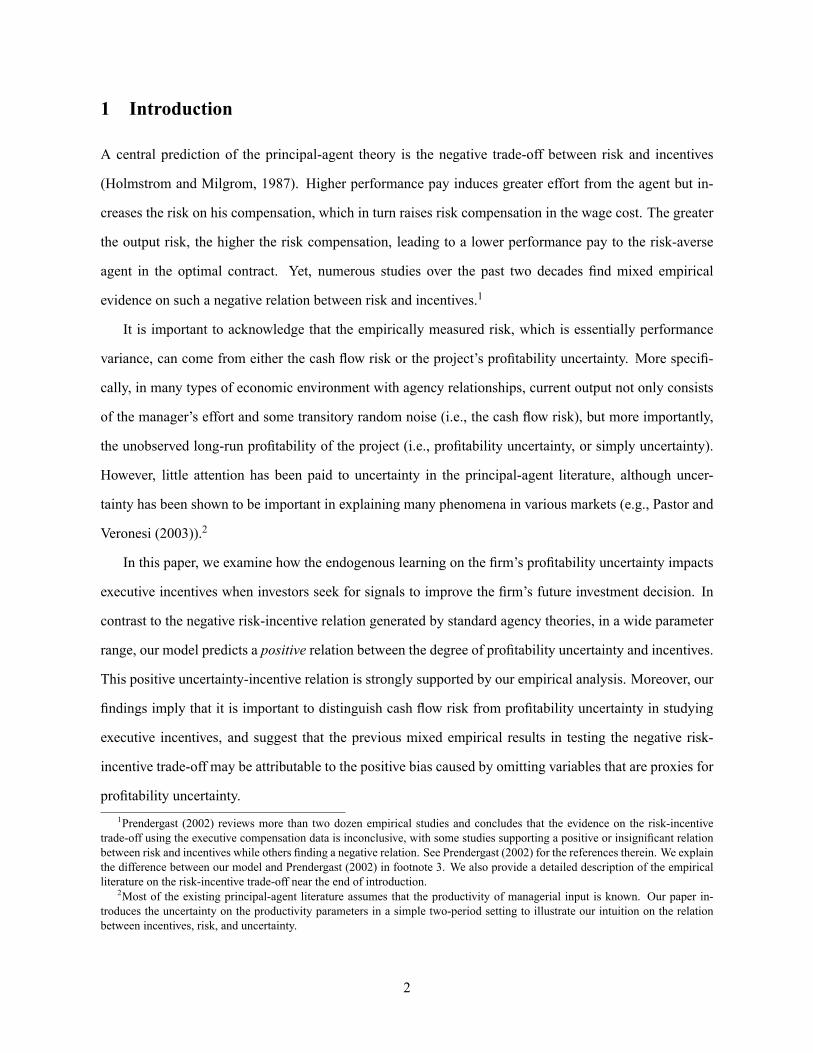
t=0 t=1 t=2

At time 0, the firm

decides whether to

take the project. If

so, the firm offers a

linear contract to

the agent.

At time 1, the agent

chooses effort and

output is realized.

At time 2, the firm

learns about and

then adjusts the

investment level.

Figure 1: Timeline of the model.

to a new capital level of 1+ I , but incurs a quadratic adjustment cost of I+ k2I2, where k > 0 is a positive

constant. As a result, investors at the beginning of period 2 will solve the following problem:

maxI;L2

E�� (1 + I + L2) + �2 �

1

2kI2 � I � l

2L22

���� y1; L�1� .In summary, the timeline of the model is as follows, as shown in Figure 1. We solve the model

backward in the following sections.

1. At the beginning of t = 1 the �rm is deciding whether to take a project with capital normalized to

1. Its outside option is normalized to zero.

2. If the �rm decides to take this project, investors hire one manager and offers him a linear contract

w1 = � + �y1, where y1 = � (1 + L1) + �1 is the project's output at period 1. Therefore the

investors' payoff at period 1 is given by

y1 � w1 � 1 = � (1 + L1) + �1 � �� �y1 � 1

3. Given the outcome y1, investors update their belief about � based on the prior � � N (�0; 0).

still persists) will share the same qualitative feature as period 1 incentives. The important assumption is that the old period 1manager is replaced by another new manager in period 2, so that the incentive contract is short-term. With long-term employmentrelationship and endogenous learning, the manager can enjoy some endogenous information rent (as the manager who shirks atperiod 1 knows that the project actually is better than what investors believe), which makes analysis complicated. See He, Yu,and Wei (2010) for details.

7

4. At t = 2, the �rm can make the capital investment I and labor investment L2, so that y2 =

� (1 + I + L2) + �2. The second period payoff is

� (1 + I + L2) + �2 � I �k

2I2 � l

2L22:

2.2 Learning and Investing in Period 2

Immediately after observing y1 at period 1, investors update their belief about �. Given the optimal labor

input L�1 implemented by the incentive contract at period 1, Bayes' rule implies that the posterior of the

project's pro�tability is characterized by the posterior mean and posterior variance:

�1 � E [� jy1; L�1 ] = �0 + 1 (1 + L

�1)

�2�[y1 � �0 (1 + L�1)] ; (3)

1 � V ar [� jy1; L�1 ] = 0�

2�

�2� + 0 (1 + L�1)2 : (4)

Intuitively, y1� �0 (1 + L�1) represents an unexpected shock from the output. Then if investors observes a

positive unexpected shock y1 � �0 (1 + L�1) > 0, which serves a positive signal to the project pro�tability

�, then as in Eq. (3) they should update the long-term pro�tability �1 upwards.

As we will see shortly, given the period 1 output information, the pro�tability estimate �1 guides the

�rm's investment decision at period 2. The posterior variance 1 in Eq. (4), which measures the precision

of pro�tability estimate �1, directly determines the investment ef�ciency at period 2. Moreover, it is

important to stress that the posterior variance 1 negatively depends on L�1, thanks to the multiplicative

structure in Eq. (1). Otherwise, a greater investment in K1 or L1 has no impact on the informativeness of

the signal y1 in learning the pro�tability �.

At period 2 the �rm makes capital investment and labor investment to solve the following problem:

V2 (�1) � maxI;L2

E�� (1 + I + L2) + �2 � I �

1

2kI2 � l

2L22 jy1; L�1

�;

= �1 +(�1 � 1)2

2k+�212l;

where we have expressed the investors' period 2 value V2 (�1) as a function of the period 1 posterior mean

�1. For instance, had the investors perfectly known �, they would have chosen the investment level ��1k .

Due to imperfect information, the optimal investment I� = �1�1k deviates from the optimal level ��1k in

the full-information setting, and the difference has a variance of 1=k2.

8

Standing at time 0, the time-0 expected payoff from period 2 is given by

E [V2 (�1)] = �0 +(1� �0)2

2k+�202l+l + k

2kl( 0 � 1) : (5)

In other words, investors' expected value in period 2 is decreasing in 1, i.e., the posterior variance of the

unobserved pro�tability �. Intuitively, the lower the posterior variance 1, the more precise the estimate

of the pro�tability �, and the more ef�cient the second period investment. Moreover, from Eq. (4), 1

decreases with effort L�1. This important observation implies that, when raising the incentive in the �rst

period, there is more information content in period 1 output y1, and hence investors learn more about the

unobservable pro�tability �. As we will elaborate on in the next section, this learning-by-doing mechanism

is the key in driving our result.

2.3 Optimal Contracting in Period 1

We now solve the model backward for Stages 2 and 1. At Stage 2, i.e., after the �rm decides to take the

project and hires a manager, we solve for the optimal linear contract, and in turn the �rm's value from this

project. Then at Stage 1, the �rm will take the project if and only if this value exceeds 0.

At Stage 2, investors offer a linear contract w1 = �+ �y1 to implement the optimal labor (effort) L�1,

and the optimal contract maximizes their expected total value (including both periods' cash �ows):

max�;�;L�1

E [y1 � w1 � 1 + V2 (�1)] ; (6)

subject to the manager's incentive compatibility and the participation constraints:

L�1 = argmaxL1

E�� exp

��a�w1 �

l

2L21

���; and E

�� exp

��a�w1 �

l

2L21

���� bU:

The following lemma gives the manager's optimal labor (effort) choice in response to the incentive contract

summarized by (�; �):

Lemma 1 A contract w1 = � + �y1 implements labor L�1 and satis�es the manager's participation

constraint if and only if

L�1 =� (�0 � a 0�)l + a 0�

2 ; (7)

and

� = ���0l + �0�

l + a 0�2 �

1

2

�2��20 + al 0

�l + a 0�

2 +1

2a�2��

2: (8)

9

0 0.5 1 1.5­0.2

­0.18

­0.16

­0.14

­0.12

­0.1

­0.08

­0.06

­0.04

­0.02

0

­γ1*

Effort L 1

γ0=0.01

γ0=0.1

γ0=0.5

γ0=1

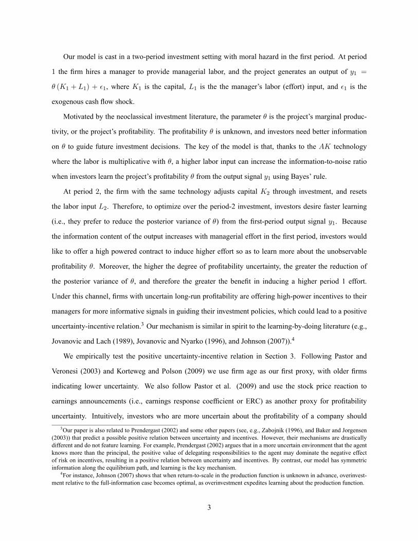
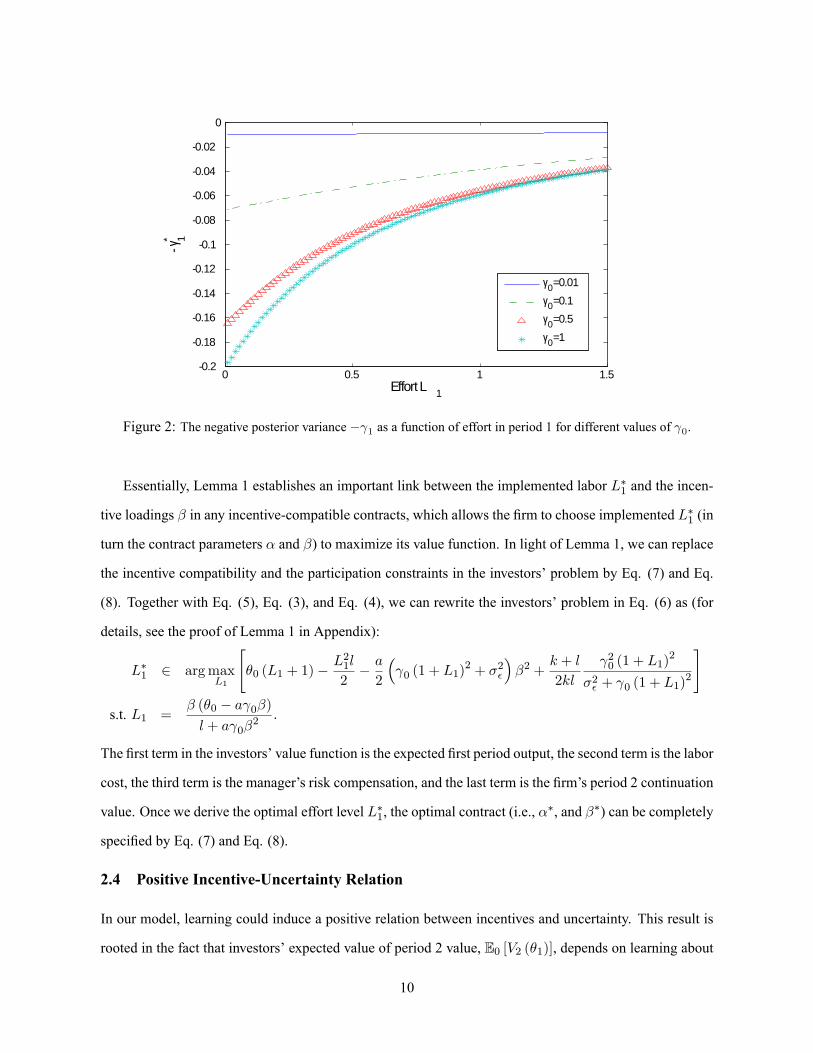
Figure 2: The negative posterior variance � 1 as a function of effort in period 1 for different values of 0.

Essentially, Lemma 1 establishes an important link between the implemented labor L�1 and the incen-

tive loadings � in any incentive-compatible contracts, which allows the �rm to choose implemented L�1 (in

turn the contract parameters � and �) to maximize its value function. In light of Lemma 1, we can replace

the incentive compatibility and the participation constraints in the investors' problem by Eq. (7) and Eq.

(8). Together with Eq. (5), Eq. (3), and Eq. (4), we can rewrite the investors' problem in Eq. (6) as (for

details, see the proof of Lemma 1 in Appendix):

L�1 2 argmaxL1

"�0 (L1 + 1)�

L21l

2� a2

� 0 (1 + L1)

2 + �2�

��2 +

k + l

2kl

20 (1 + L1)2

�2� + 0 (1 + L1)2

#

s.t. L1 =� (�0 � a 0�)l + a 0�

2 :

The �rst term in the investors' value function is the expected �rst period output, the second term is the labor

cost, the third term is the manager's risk compensation, and the last term is the �rm's period 2 continuation

value. Once we derive the optimal effort level L�1, the optimal contract (i.e., ��, and ��) can be completely

speci�ed by Eq. (7) and Eq. (8).

2.4 Positive Incentive-Uncertainty Relation

In our model, learning could induce a positive relation between incentives and uncertainty. This result is

rooted in the fact that investors' expected value of period 2 value, E0 [V2 (�1)], depends on learning about

10

pro�tability � from period-1 output y1. As indicated by Eq. (5), maximizing E0 [V2 (�1)] is equivalent to

minimizing the posterior variance of �, i.e., 1. Because L1 is multiplicative with � in the signal y1 as in

(1), implementing a higher effort L1 raises the informativeness of the period 1 signal y1, or equivalently,

reduces the posterior variance 1. Essentially, this mechanism shares the similar spirit to the learning-by-

doing literature (e.g., Jovanovic and Lach (1989), Jovanovic and Nyarko (1996), and Johnson (2007)). For

example, Johnson (2007) shows that when there is uncertainty about �rms' production function, �rms tend

to overinvest due to the desire to learn about the unknown production function.

Presumably, this learning-by-doing effect is stronger in a more uncertain environment (i.e., a larger 0).

This is because starting with a larger 0, the reduction of the posterior variance will be more signi�cant,

which results in a greater bene�t of inducing a higher effort. That is, based on Eq. (4), we have

@2 (� 1)@L�1@ 0

> 0:

In Figure 2, we plot � �1 as a function of effort L1 for different levels of 0. As we can see, when

0 increases, the marginal bene�t of raising effort L1 becomes greater. To implement a higher effort, a

greater incentive �� is needed, which results in a positive relation between uncertainty and incentives.

In Proposition 1 we formally prove the existence of such a positive uncertainty-incentive relation when

the manager is suf�ciently risk tolerant. Notice that high uncertainty also implies a greater incentive

provision cost, since uncertainty raises the risk that the manager is bearing. This is the reason why we

require the manager to be suf�ciently risk tolerant.

Proposition 1 For suf�ciently small risk aversion coef�cient a, a positive relation exists between �� and

0, i.e.,d��

d 0> 0.

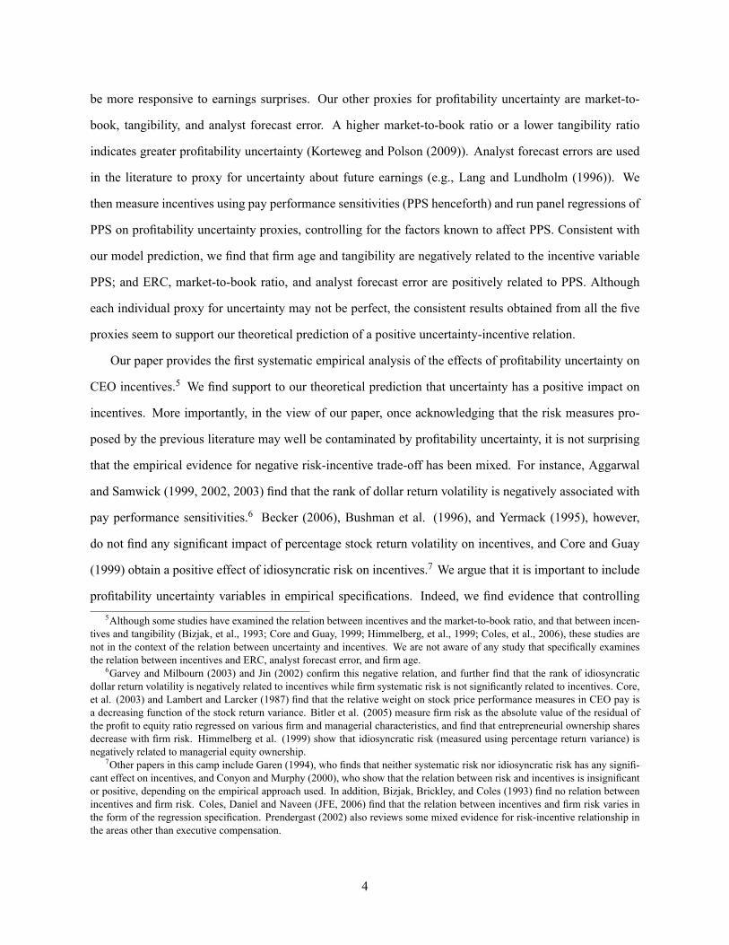
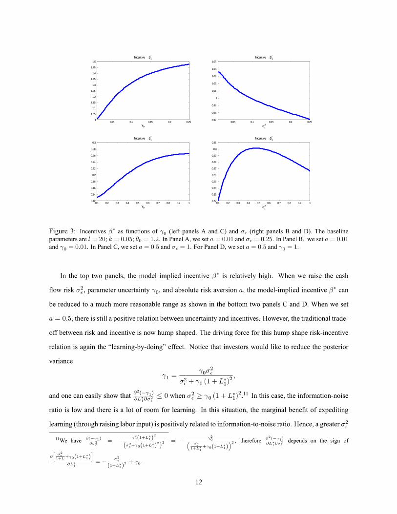
Figure 3 plots the incentive �� as a function of both uncertainty 0 and risk �2� . Here, we vary the

pro�tability uncertainty 0 in the left panels (Panel A and C) and the cash �ow risk �2� in the right panels

(Panel B and D). We set absolute risk aversion a = 0:01 for the top two panels.10 In Panel A (B), we vary

0 (�2� ) from 0 to 0.25. Panel B gives the traditional negative trade-off between risk �2� and incentives ��.

However, as predicted by Proposition 1, Panel A gives a positive relation between pro�tability uncertainty

0 and incentive ��.10Given CEOs are relatively wealthy, it is reasonable to choose a small absolute risk aversion coef�cient since a �Wealth

is the relative risk aversion coef�cient. As suggested by Proposition 1, if we raise the risk aversion coef�cient a, the relationbetween parameter uncertainty and incentives can be reversed. However, for a reasonably small risk aversion coef�cient, wegenerally obtain a positive relation between uncertainty and incentives.

11

0.05 0.1 0.15 0.2 0.251

1.05

1.1

1.15

1.2

1.25

1.3

1.35

1.4

1.45

1.5

γ0

Incentive β*1

0.05 0.1 0.15 0.2 0.250.97

0.98

0.99

1

1.01

1.02

1.03

1.04

1.05

σε2

Incentive β*1

0.1 0.2 0.3 0.4 0.5 0.6 0.7 0.8 0.9 10.12

0.14

0.16

0.18

0.2

0.22

0.24

0.26

0.28

0.3

γ0

Incentive β*1

0.1 0.2 0.3 0.4 0.5 0.6 0.7 0.8 0.9 10.22

0.23

0.24

0.25

0.26

0.27

0.28

0.29

0.3

0.31

σε2

Incentive β*1

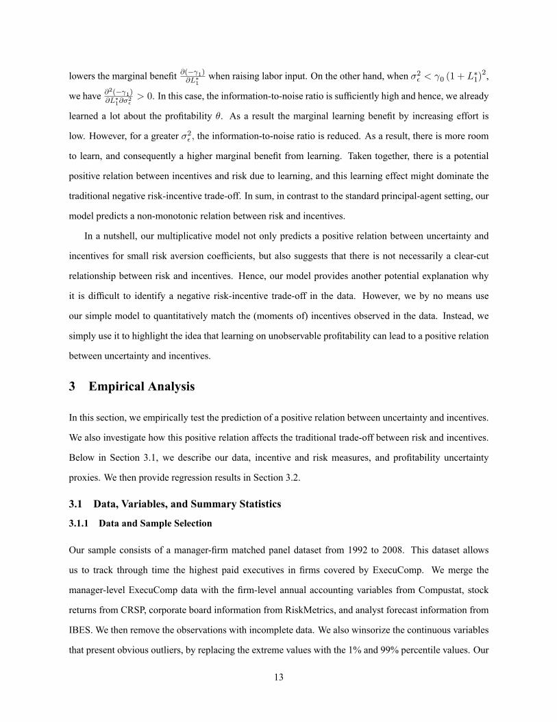
Figure 3: Incentives �� as functions of 0 (left panels A and C) and �� (right panels B and D). The baselineparameters are l = 20; k = 0:05; �0 = 1:2. In Panel A, we set a = 0:01 and �� = 0:25. In Panel B, we set a = 0:01and 0 = 0:01. In Panel C, we set a = 0:5 and �� = 1. For Panel D, we set a = 0:5 and 0 = 1.

In the top two panels, the model implied incentive �� is relatively high. When we raise the cash

�ow risk �2� , parameter uncertainty 0, and absolute risk aversion a; the model-implied incentive �� can

be reduced to a much more reasonable range as shown in the bottom two panels C and D. When we set

a = 0:5; there is still a positive relation between uncertainty and incentives. However, the traditional trade-

off between risk and incentive is now hump shaped. The driving force for this hump shape risk-incentive

relation is again the �learning-by-doing� effect. Notice that investors would like to reduce the posterior

variance

1 = 0�

2�

�2� + 0 (1 + L�1)2 ;

and one can easily show that @2(� 1)@L�1@�

2�� 0 when �2� � 0 (1 + L�1)

2.11 In this case, the information-noise

ratio is low and there is a lot of room for learning. In this situation, the marginal bene�t of expediting

learning (through raising labor input) is positively related to information-to-noise ratio. Hence, a greater �2�

11We have @(� 1)@�2�

= � 20(1+L�1)

2��2�+ 0(1+L�1)

2�2 = � 20�

�2�1+L�1

+ 0(1+L�1)�2 , therefore @2(� 1)

@L�1@�2�depends on the sign of

@

��2�1+L

+ 0(1+L�1)�

@L�1= � �2�

(1+L�1)2 + 0:

12

lowers the marginal bene�t @(� 1)@L�1when raising labor input. On the other hand, when �2� < 0 (1 + L�1)

2,

we have @2(� 1)@L�1@�

2�> 0. In this case, the information-to-noise ratio is suf�ciently high and hence, we already

learned a lot about the pro�tability �. As a result the marginal learning bene�t by increasing effort is

low. However, for a greater �2� ; the information-to-noise ratio is reduced. As a result, there is more room

to learn, and consequently a higher marginal bene�t from learning. Taken together, there is a potential

positive relation between incentives and risk due to learning, and this learning effect might dominate the

traditional negative risk-incentive trade-off. In sum, in contrast to the standard principal-agent setting, our

model predicts a non-monotonic relation between risk and incentives.

In a nutshell, our multiplicative model not only predicts a positive relation between uncertainty and

incentives for small risk aversion coef�cients, but also suggests that there is not necessarily a clear-cut

relationship between risk and incentives. Hence, our model provides another potential explanation why

it is dif�cult to identify a negative risk-incentive trade-off in the data. However, we by no means use

our simple model to quantitatively match the (moments of) incentives observed in the data. Instead, we

simply use it to highlight the idea that learning on unobservable pro�tability can lead to a positive relation

between uncertainty and incentives.

3 Empirical Analysis

In this section, we empirically test the prediction of a positive relation between uncertainty and incentives.

We also investigate how this positive relation affects the traditional trade-off between risk and incentives.

Below in Section 3.1, we describe our data, incentive and risk measures, and pro�tability uncertainty

proxies. We then provide regression results in Section 3.2.

3.1 Data, Variables, and Summary Statistics

3.1.1 Data and Sample Selection

Our sample consists of a manager-�rm matched panel dataset from 1992 to 2008. This dataset allows

us to track through time the highest paid executives in �rms covered by ExecuComp. We merge the

manager-level ExecuComp data with the �rm-level annual accounting variables from Compustat, stock

returns from CRSP, corporate board information from RiskMetrics, and analyst forecast information from

IBES. We then remove the observations with incomplete data. We also winsorize the continuous variables

that present obvious outliers, by replacing the extreme values with the 1% and 99% percentile values. Our

13

full sample includes 2,441 �rms and 25,999 top executives who have worked for these companies, and the

main regressions are estimated based on this full sample.

3.1.2 Pay-Performance Sensitivity

The dependent variable in the paper is pay-performance sensitivity (PPS), a standard variable used in the

literature to measure managerial incentives. The literature on executive compensation typically employs

two measures of PPS. The �rst measure, the dollar-to-dollar measure (PPS1), is equal to the dollar change

in stock and option holdings for a one dollar change in �rm value (see, e.g., Aggarwal and Samwick

(2003), Jin (2002), Palia (2001), and Yermack (1995)).12 This measure is essentially @Wealth=@(Market

V alue) (whereWealth is the CEO's wealth) and is also called value-sensitivity or share of the money in

Becker (2006). Another measure, the dollar-to-percentage measure (PPS2), is equal to the dollar change

in stock and option holdings for a one percent change in �rm value (Core and Guay (2002)). The PPS2

measure is equal to @Wealth=@(Return) and is also referred to as return-sensitivity or money at stake in

Becker (2006).

Baker and Hall (2004) mention that both PPS measures may be appropriate, depending on how CEO

actions are assumed to affect �rm value. When CEO actions primarily affect �rm dollar returns and have

constant dollar effects across �rms of different sizes (such as perquisite consumption through the purchase

of a corporate jet), the appropriate measure of CEO incentives is dollar-to-dollar. In contrast, when CEO

actions have an impact proportional to �rm size and thus primarily affect �rm percentage returns (such as

the implementation of �rm strategy), the appropriate measure of CEO incentives is dollar-to-percentage.

Baker and Hall (2004) estimate the marginal product of CEO effort and �nd that neither polar case as-

sumption is correct: the marginal product of CEO effort scales with �rm size in varying degrees. They

interpret the results as evidence that CEOs participate in a range of activities. As a result, similar to Becker

(2006) and Core and Guay (1999), we use both measures of PPS in our empirical analysis.

The two PPSmeasures mentioned above are standard measures employed in the extant literature, which

include Aggarwal and Samwick (2003), Becker (2006), Core and Guay (2002), etc. In addition to these

two direct measures of incentives, some empirical studies use a regression approach to obtain PPS. In this12Jensen and Murphy (1990) measure PPS as the change in a CEO's total wealth resulting from a $1000 increase in shareholder

value. The total wealth includes �nancial wealth and capitalized future labor income. Hall and Liebman (1998) argue thatchanges in CEO's �nancial wealth account for nearly all of the PPS value. Furthermore, �nancial wealth can be measuredrelatively precisely compared to capitalized future labor income. Therefore, we focus our analysis on PPS calculated from aCEO's �nancial wealth.

14

approach, executives' wealth is regressed on �rm performance and other �rm characteristic variables, and

the coef�cient on �rm performance is interpreted as the pay-performance sensitivity (see e.g., Aggarwal

and Samwick (1999), Garvey and Milbourn (2003), and Jensen and Murphy (1990)). Differing from such

regression technique that derives a single estimate of the average pay-performance link, the direct approach

calculates PPS1 and PPS2 for each individual executive and obtains a distribution of incentives. We also

replicate our empirical analysis using the PPS obtained from the regression approach and we achieve

essentially the same results.13

3.1.3 Empirical Proxies for Pro�tability Uncertainty

The primary explanatory variables of interest in the paper are �ve pro�tability uncertainty variables. These

variables have been used in the existing literature (Pastor and Veronesi, 2003; Korteweg and Polson, 2009)

as proxies for pro�tability uncertainty. Below we explain the �ve proxies, and we also include the detailed

de�nitions of these variables in Appendix B. It is worth noting that the results of the paper should be

interpreted with the following points in mind. First, the uncertainty proxies are not perfect; they could

re�ect �rm characteristics other than pro�tability uncertainty. It is, therefore, important to investigate an

array of uncertainty variables commonly used in the literature and see whether all these variables give

consistent results. Second, some of the uncertainty variables we use are positively correlated with �rm

volatility; others are negatively correlated with volatility. Examining all the different uncertainty variables

will help us separate the role of uncertainty from that of volatility. Furthermore, we do not use �rm size

as an uncertainty proxy, although it is proposed by such literature as Korteweg and Polson (2009). There

exists a strong empirical relation between size and PPS; that is, �rm size is negatively correlated with

PPS1 and positively correlated with PPS2 (e.g., Edmans, et al., 2009). The literature has proposed various

explanations for this pattern, and therefore size may not be a clean pro�tability uncertainty variable for

our purpose. 14 We do, however, include �rm size in all our regressions as a control variable to capture the13Using the regression approach, the coef�cient of the cross term of �rm performance and variable X can be interpreted as the

marginal effect of X on PPS. We �nd that the coef�cients of the cross terms of �rm performance and the uncertainty variables areconsistent with our expectations. We also �nd that the coef�cient of the cross term of �rm performance and volatility becomesgenerally negative when the uncertainty variables are captured.

14For instance, in the Holmstrom and Milgrom's CARA-Normal framework, risk is measured in dollar returns. Then dollar-to-dollar PPS1 should be lower for larger �rms with greater dollar variances in output. For the dollar-to-percentage PPS2 meaure,the matching model in Gabaix and Landier (2008) suggests that pay increases with �rm size. Since part of compensation is invariable pay, it suggests that PPS2 is positively correlated with �rm size.

15

size effect.15

Natural log of �rm age The �rst proxy that we employ is �rm age. Previous studies such as Pastor

and Veronesi (2003) and Korteweg and Polson (2009) use �rm age as a proxy for pro�tability uncertainty.

Uncertainty declines over a �rm's lifetime due to learning, and younger �rms have higher uncertainty.

Following Pastor and Veronesi (2003), we consider each �rm as �born� in the year of its �rst appearance

in the CRSP database. Speci�cally, we obtain the �rst occurrence of a valid stock price on CRSP, as well

as the �rst occurrence of a valid market value in the CRSP/COMPUSTAT database, and take the earlier

of the two. The �rm's age is assigned the value of one in the year in which the �rm is born and increases

by one in each subsequent year. As in Pastor and Veronesi (2003), we take the natural log of �rm age.

Log(age) is concave in �rm's plain age, and this is to capture the idea that regarding uncertainty, one year

of age should matter more for young �rms than for old �rms.16

Earnings response coef�cient (ERC) In constructing our second proxy for pro�tability uncertainty, we

follow Pastor et al. (2009) and Cremers and Yan (2010), and use the stock price reaction to earnings

announcements (i.e., earnings response coef�cient or brie�y, ERC). Intuitively, investors who are more

uncertain about the pro�tability of a company should respond more strongly to earnings surprises. Pastor

et al. (2009) propose two ERC measures (ERC1 and ERC2). ERC1 is the average of a �rm's previous 12

stock price reactions to quarterly earnings surprises, and ERC2 is the negative of the regression slope of the

�rm's last 20 quarterly earnings surprises on its abnormal stock returns around earnings announcements.

Appendix B provides more details on the ERC variable. We report in the paper the results from using the

ERC1 variable and the results from the ERC2 variable are similar and available upon request. As noted in

Pastor et al. (2009), the ERC measure is ideal to separate uncertainty from volatility because ERC is high

when uncertainty is high and when earnings volatility is low. When realized earnings are more precise,15We also decide not to use some other uncertainty proxies in the literature. Baker andWurgler (2006) provide some proxies for

hard-to-value stocks. Besides the variables we mention above, they mention that non-dividend-paying stocks are harder to valuethan dividend-paying stocks because the value of a �rm with stable dividends is less subjective. As a result, dividend-paying �rmspossibly have lower uncertainty and thus may be related to lower incentives. We do see a consistent negative association betweenthe dividend-paying indicator and PPS in our regressions. An alternative explanation of the negative association is that �rms withcash constraints (such as non-dividend-paying companies) might prefer restricted stock and options over cash compensation. Asa result, a higher PPS is more likely to be observed among non-dividend payers (Jin (2002) and Yermack (1995)). We include thedividend-paying indicator as a control variable in all model speci�cations.

16Pastor and Veronesi (2003) also use the negative of the reciprocal of one plus the �rm age. Using this measure, we �ndsimilar results.

16

investors would react more to earnings surprises, leading to a higher value of ERC. The shortcoming of

the ERC measure is its measurement error. As a result, we also incorporate other empirical proxies of

uncertainty in the analysis.

Market-to-book ratio The third proxy for pro�tability uncertainty is the market-to-book ratio, which

equals market value of equity plus the book value of debt, divided by total assets. Pastor and Veronesi

(2003) show that aging in the life of a �rm is accompanied by a decrease in the market-to-book ratio.

According to Korteweg and Polson (2009), the market-to-book ratio is a proxy for �rm growth opportu-

nities, and such opportunities are inherently more dif�cult to value than the assets in place. As a result,

the market-to-book ratio increases with the uncertainty about �rm pro�tability. We acknowledge that the

market-to-book ratio may capture �rm growth and other characteristics in addition to uncertainty. An in-

vestigation of the market-to-book ratio may not be a direct test of the impact of uncertainty on incentives. It

is thus important to also examine a variety of other uncertainty proxies and see whether all these variables

give consistent results. Hence, our results need to be interpreted with this point in mind.

Tangibility The fourth proxy is tangibility. Korteweg and Polson (2009) mention that �rms with more

tangible assets (property, plant, and equipment) are easier to value and thus are related to lower pro�tability

uncertainty. We use net property, plant, and equipment scaled by �rm total assets to measure tangibility.

Analyst forecast error We also construct an analyst forecast error variable as a proxy of pro�tability

uncertainty. Based on Bae et al. (2008) and Lang and Lundholm (1996), for each speci�c company in each

�scal year, we �rst obtain the absolute value of the forecast error made by each analyst, where forecast

errors are de�ned as the difference between the forecast value and the actual value of earnings per share.

We then use the median value of these absolute forecast errors, scaled by the absolute value of the actual

EPS. Using the mean value of the absolute forecast errors gives similar results.17

17Another widely used measure based on IBES data is analysts' forecast dispersion, which usually proxies for potential dis-agreement in the market. The difference between forecast dispersion and forecast error is that the latter considers the distancebetween EPS forecast and actual EPS, while the former considers the distance between EPS forecast and the mean forecast amonganalysts. The forecast error variable better captures pro�tability uncertainty studied in this paper. Consider the situation wheretwo analysts issued the same EPS forecast of $5, and the actual EPS turns out to be $3. Then in this example the forecast errorwill be 2 (which might result from large uncertainty), but the forecast dispersion is just 0.

17

3.1.4 The Risk Variable

Similar to the literature that tests the relation between risk and incentives, we include stock return volatility

as a measure of risk in our regression analysis. As mentioned earlier, existing theories predict a negative

relation between risk and incentives, but the empirical evidence on this aspect is inconclusive. Our paper

re-examines this issue empirically, with uncertainty variables being included in the empirical speci�cation.

We measure stock return volatility as the standard deviation of daily log (percentage) returns over the past

�ve years, which is then annualized by multiplying by the square root of 254 (Yermack (1995) and Palia

(2001)). We also use the percentage rank of stock dollar return variance (Aggarwal and Samwick (1999,

2002, 2003); Garvey and Milbourn (2003); and Jin (2002)) in the empirical analysis, we obtain essentially

the same results.

3.1.5 Control Variables

In the regressions, we include various control variables that could potentially affect the incentives provided

by a �rm to its managers. These control variables have been used in the empirical literature on the deter-

minants of managerial incentives (Aggarwal and Samwick (2003); Core et al. (1999); Jin (2002); Palia

(2001); etc.). As mentioned at the beginning of Section 3.1.3, since there is well-established empirical

pattern between incentives and �rm size, we �rst include �rm size as a control. Following the literature,

we also include pro�tability, the ratio of capital expenditure to total assets, advertising expenses scaled by

total assets, a dummy variable that is set to one whenever advertising expenses are missing, �rm leverage,

and dividend payout indicator. We further control for corporate governance variables, which include the

CEO chair indicator and the proportion of inside directors in the board. Manager-level variables, such as

log(tenure), the CEO indicator, and the female indicator, are also controlled in the regressions. Finally,

year and industry effects are included to capture the time and industrial differences in the level of man-

agerial incentives. The detailed de�nitions of all the variables used in the paper are described in Appendix

B.

3.1.6 Summary Statistics and Correlations between Variables

Table 1 contains summary statistics of the variables used in the regression analysis. The average (median)

dollar-to-dollar measure of PPS is 1.13% (0.22%), suggesting that the average (median) dollar change in

the sample executives' stock and option holdings for a one thousand dollar change in �rm value is $11.3

18

($2.2). The summary statistics on the dollar-to-percentage measure of PPS show that the average (median)

dollar change in the executives' stock and option holdings for a 1% change in �rm (equity) value is $168.61

($27.97) thousand. These summary numbers are consistent with those provided in the empirical literature

such as Core and Guay (1999), Palia (2001), and Yermack (1995). The statistics also imply a positive

skewness in PPS, with a few companies having very high incentives.

The average, median, minimum, and maximum age of the sample �rms is 26, 20, 1, and 84 years,

similar to those reported in Pastor and Veronesi (2003). The �rms in the sample have an average (median)

earnings response coef�cient of 4.44 (2.88), market-to-book ratio of 2.08 (1.51), tangibility of 0.29 (0.23),

and total assets of $6.6 ($1.3) billion. The average analyst forecast error relative to the actual value is

about 16%. In addition, the average (median) annual stock return volatility is 44% (39%).

Table 2 examines the pairwise correlations between the variables. The two PPS variables have a

correlation coef�cient of 0.55. The PPS1 variable is negatively correlated with �rm age and tangibility,

and is positively correlated with the earnings response coef�cient (ERC) and the market-to-book ratio. The

correlations between PPS2 and �rm age are very low; it may be due to the fact that PPS2 is PPS1 times

market value of equity, and the negative relation between age and PPS1 is canceled out by the positive

relation between age and market value. When we control for �rm size in the model, the relation between

PPS2 and �rm age becomes negative and signi�cant.

Table 2 also shows that the uncertainty proxy variables are correlated with each other, with the correla-

tion between �rm age and market to book being -0.23 and the correlation between �rm age and tangibility

around 0.18. This indicates that younger �rms tend to be the �rms with more growth options and lower

tangibility ratios. The table also reveals very low correlations between ERC and volatilities and between

ERC and �rm size. This suggests that ERC serves an ideal proxy variable that separates uncertainty from

volatility and �rm size. On the other hand, the percentage return volatilities and the dollar return volatili-

ties have opposite signs in correlations with other variables. This is perhaps due to the fact that the dollar

return volatility, which equals percentage return volatility multiplied by �rm market value, captures the

�rm size effect.

19

3.2 Empirical Results

This section uses regression analysis to examine the effect of pro�tability uncertainty and risk on incen-

tives. The main empirical model is as follows:

PPSijt = �+ �1(Uncertainty proxies)j;t�1 + �2(Risk)j;t�1 (9)

+�3(Firm characteristics)j;t�1 + �4(Managerial characteristics)i;t�1

+�5(Y ear indicators)t + �6(Industry indicators)j + �ijt:

In the equation, we use i to denote manager, j to denote �rm, and t to denote year. The dependent variable

is the dollar-to-dollar measure (PPS1) and the dollar-to-percentage measure (PPS2) of pay-performance

sensitivities. In the OLS regressions, we control for industry effects using two digit SIC indicator variables.

In the �rm-manager pair �xed effects regressions, we replace industry effects with �rm-manager �xed

effects in Eq. (9) as the latter absorbs the former. We lag all the explanatory variables by one year to

mitigate potential reverse causality issue. We, however, acknowledge that lagging may not fully resolve

endogeneity because serial correlations may exist in some explanatory variables. We thus also use the

�xed effects model in robustness analysis to deal with the endogeneity problem caused by time-invariant

unobservable factors.

3.2.1 Main Results

Tables 3 and 4 report the OLS regression results, with Table 3 having PPS1 as the dependent variable and

Table 4 having PPS2. The t-statistics in these regressions are heteroskedasticity robust and are adjusted

for clustering within �rms. In both tables, Column (1) does not include any of the �ve uncertainty vari-

ables, Columns (2)-(6) include one of the �ve uncertainty variables, and Column (7) include all the �ve

uncertainty variables.

Positive uncertainty-incentive relation The results in both Tables 3 and 4 show that �rm age is neg-

atively related to incentives (Columns (2) and (7)), indicating that younger �rms, i.e., �rms with higher

uncertainty, are associated with greater managerial incentives. Both the earnings response coef�cient

(ERC) and the market-to-book ratio are positively associated with the incentive variable. The relation be-

tween tangibility and PPS is negative, suggesting that �rms that have more tangible assets are associated

with lower incentives. Firms with greater analyst forecast errors (that might be due to greater uncertainty)

20

are also shown to give higher incentives to executives (although this coef�cient is insigni�cant in the

PPS2 regressions in Table 4). All these results indicate a positive relation between pro�tability uncertainty

and incentives, as predicted by our model. This positive relation is not only statistically signi�cant but

also economically important. Take Table 3 Column (7) and Table 4 Column (7) as examples. A one-

standard-deviation decrease in log(�rm age), which is about 0.97 (i.e., �rm age reduces by about 3 years),

is associated with an increase of approximately 0.23% (=0.97�0.24) in PPS1 and 36.16 (=0.97�37.28) in

PPS2. These values are of similar magnitude to that of the sample median level of PPS. Other uncertainty

variables have similar economic signi�cance.

Re-examine the risk-incentive relation Controlling for pro�tability uncertainty can help reveal the

negative risk-incentive relation, a key prediction from standard agency theories but with mixed empirical

support from existing literature. From the point of view of this paper, the risk proxies used in the previous

literature, namely stock volatility and rank of dollar return volatility, could be contaminated by pro�tability

uncertainty. If pro�tability uncertainty is positively related to incentives, then it is not surprising that pre-

vious research, in which the risk proxy captures both the cash �ow risk �2� and the pro�tability uncertainty

0, �nds ambiguous risk-incentive relation.

The above reasoning suggests that in revealing the negative risk-incentive relation, it is important to

control for uncertainty, as this helps correct for the positive bias potentially caused by omitting relevant

variables that are proxies for pro�tability uncertainty. Our empirical results offer evidence for this impli-

cation. In columns (1) of Tables 3 and 4, when we do not include the uncertainty proxies, stock return

volatility is positively related to incentives. This result, which seems odd based on the standard agency

theory, is actually consistent with the �ndings in some empirical studies that document a positive relation

between volatility and incentives (Prendergast (2002), Core and Guay (1999), and Conyon and Murphy

(2000)).

In columns (7) of Tables 3 and 4, when we include the uncertainty variables in the regressions, the

relation between volatility and incentives changes from signi�cantly positive to either insigni�cantly pos-

itive in the PPS1 regression, or to insigni�cantly negative in the PPS2 regression. This pattern generally

hold in other speci�cations considered in Section 3.2.2 for robustness checks. Although our results do not

fully restore the signi�cantly negative risk-incentive relation from the data (possibly due to such reasons

as endogenous matching between �rm risk and CEO's risk appetite, the learning-by-doing effect in Figure

21

3 Panel D in this paper, etc.), it should be safe to say that separating pro�tability uncertainty from cash

�ow risk is important when empirically examining the negative risk-incentive relation. Our results also

indicate that it may be important to separate the effect of pro�tability uncertainty from that of risk when

studying other corporate variables.

Relation between investment volatility and uncertainty In Table 5 we regress the volatility of quar-

terly investment-to-capital ratio (quarterly capital expenditure scaled by previous quarter-end net property,

plant, and equipment, see Cleary (1999) and Kaplan and Zingales (1997)) on the same explanatory vari-

ables as in Eq. (9). Under the �learning-by-doing� mechanism in our model, �rms with uncertain long-run

pro�tability are offering high-power incentives to their managers for more informative signals in guiding

their investment policies. One immediate check of this �learning-by-doing� channel, without involving

executive incentives, is to investigate whether �rms with higher uncertainty indeed have higher investment

volatilities. As expected, both the correlations in Table 2 and the regression in Table 5 show that investment

volatility is increasing in the uncertainty proxies, which offers support to our mechanism.

3.2.2 Robustness Analysis

This section performs additional analysis to investigate the robustness of our empirical results.

Risk measured as dollar return volatility In addition to measuring �rm risk using the variance of stock

percentage returns, we attempt a different measure of �rm risk: volatility of stock dollar returns. Following

Aggarwal and Samwick (1999, 2003) and Jin (2002), we use the percentage rank of the variance of dollar

returns. According to Aggarwal and Samwick (1999, 2003), the use of the percentage ranks deals with

potential outliers in the dollar return data and also allows the pay-performance incentives at different points

in the distribution of �rm risk to be easily compared.18 The OLS regression results using the rank of dollar

return volatility are reported in Panel A of Table 6. In Column (1), we �nd that the rank of dollar return

volatility is negative and signi�cant. This result is consistent with the �ndings in the previous studies

that use the rank of dollar return volatility as the measure of �rm risk (Aggarwal and Samwick (1999,

2002, 2003), Garvey and Milbourn (2003), and Jin (2002)). In Column (2), we include the uncertainty

variables in the model. The coef�cients of the uncertainty proxy variables have signs that are consistent18In the regressions, we also use an alternative transformation of the raw dollar return variance, namely the logarithm of dollar

return variance, and we �nd basically the same results.

22

with our theoretical prediction. Younger and less tangible growth �rms and �rms with greater analyst

forecast errors are associated with higher incentives. In Column (2), the dollar return volatility continues

to be negative and signi�cant after the uncertainty variables are included in the model. In Columns (3)

and (4), the dollar-to-percentage PPS is the dependent variable and we continue to �nd that �rms with

greater uncertainty provide higher incentives to their executives. The effect of the risk variable is positive

and signi�cant when the uncertainty variables are excluded, but the effect becomes negative (although

insigni�cant) when the uncertainty variables are introduced to the model.

Incentives measured as wealth-performance sensitivity Edmans et al. (2009) proposed an alternative

incentive measure: scaled wealth-performance sensitivity (WPS). Speci�cally, this sensitivity measure

equals the dollar change in executive wealth for a 100 percentage point change in �rm value, divided by

annual �ow compensation. This incentive measure is similar to the percentage-to-percentage incentives

used in Murphy (1985), Gibbons and Murphy (1992), and Rosen (1992), but replaces �ow compensation

in the numerator of the Murphy (1985) measure with the change in the executives' wealth. By considering

the change in wealth, the scaled wealth-performance sensitivity captures the important incentives from

changes in the value of previously granted stock and options. In Panel B of Table 6, we perform regressions

with the dependent variable being WPS and �nd that our results remain intact.

Median regressions Aggarwal and Samwick (1999, 2003) and Jin (2002) use median regressions to deal

with outliers and the right skewness in the compensation data. Following this literature, we use median

regressions and report the results in Panel C of Table 6 (with risk measured by the percentage return

volatility) and Panel D of Table 6 (with risk measured by the rank of dollar return volatility). Both tables

show that in general, uncertainty is positively related to incentives. When the dollar-to-dollar PPS is the

dependent variable, the coef�cient of the risk variable becomes less positive in Panel C and more negative

in Panel D if pro�tability uncertainty is captured in the model (see Columns (1) and (2) of both tables).

The dollar-to-percentage PPS regression gives similar results.

Fixed effect regressions In Panel E of Table 6, we run the regressions by adding the �rm-manager paired

�xed effects. Fixed effects are to deal with potential endogeneity issues. For example, it is possible that

some unobservable managerial attributes (e.g., risk aversions) are correlated with the explanatory variables

23

such as �rm age and at the same time are correlated with the dependent variable, PPS. The �rm-manager

�xed effect may also capture time-invariant unobservable factors that potentially affect endogenous match-

ing between the �rm and the manager (Graham, et al., 2010). We can see from Panel E that our main results

remain similar. The coef�cients on the pro�tability uncertainty proxies continue to show a positive relation

between pro�tability uncertainty and incentives.

Other robustness checks Finally, the tables reported so far examine each top executive's incentives.

In untabulated analysis, we also examine the CEO incentives only, and the average incentives for top

executives in each individual company. The results, omitted for brevity, provide the same implications

as those reported here. In all, the empirical results that we obtain offer strong support to our theoretical

prediction that pro�tability uncertainty is positively related to incentives.19

4 Conclusion

This paper introduces pro�tability uncertainty into an agency model, and investigates the relation between

pro�tability uncertainty and incentives. Our model predicts a positive uncertainty-incentive relation, in

contrast to the negative risk-incentive trade-off obtained in the extant literature. Therefore, it is important

to distinguish risk from uncertainty in studying CEO incentives. Using several proxies for pro�tability

uncertainty, we then empirically test and �nd strong support for our theoretical prediction. Our study

suggests that the mixed empirical results from testing the risk-incentive trade-off may be attributable to a

positive bias caused by the omission of relevant variables that are proxies for pro�tability uncertainty.

References

Aggarwal, Rajesh K., and Andrew A. Samwick, 1999, The other side of the trade-off: The impact of riskon executive compensation, Journal of Political Economy 107-1, 65�105.

Aggarwal, Rajesh K., and Andrew A. Samwick, 2002, The other side of the trade-off: The impact of riskon executive compensation - A reply, Working Paper, Dartmouth College.

19Jin (2002) mentions that past stock returns and current period PPS could be related. For example, when �rms suffer adverseshocks in previous years, they might decrease PPS to protect their executives from the adverse effect on their �nancial wealth. Inour model speci�cations, we control for lagged one-year �rm pro�tability. If we further include lagged one-year stock returns inthe model (by including lagged dollar returns when the dependent variable is the dollar-to-dollar PPS and including lagged per-centage returns when the dependent variable is the dollar-to-percentage PPS), we �nd that past stock returns have a signi�cantlypositive impact on incentives and that all our main results remain intact.

24

Aggarwal, Rajesh K., and Andrew A. Samwick, 2003, Performance incentives within �rms: The effect ofmanagerial responsibility, Journal of Finance 58-4, 1613�1650.

Bae, Kee-Hong, Rene M. Stulz, and Hongping Tan, 2008, Do local analysts know more? A cross-countrystudy of the performance of local analysts and foreign analysts, Journal of Financial Economics 88-3,581�606.

Baker, George P., and Brian J. Hall, 2004, CEO incentives and �rm size, Journal of Labor Economics 22-4,767�798.

Baker, George P., and Bjorn Jorgensen, 2003, Volatility, noise and incentives, mimeo, Harvard Universityand Columbia University.

Baker, Malcolm, and Jeffrey Wurgler, 2006, Investor sentiment and the cross-section of stock returns,Journal of Finance 61-4, 1645�1680.

Becker, Bo, 2006, Wealth and executive compensation, Journal of Finance 61-1, 379�397.

Bitler, Marianne P., Tobias J. Moskowitz, and Annette Vissing-Jorgensen, 2005, Testing agency theorywith entrepreneur effort and wealth, Journal of Finance 60-2, 539�576.

Bizjak, John M., James A. Brickley, and Jeffrey L. Coles, 1993, Stock-based incentive compensation andinvestment behavior, Journal of Accounting and Economics 16, 349�372.

Bushman, Robert M., Raf� J. Indjejikian, and Abbie Smith, 1996, CEO compensation: The role of indi-vidual performance evaluation, Journal of Accounting and Economics 21-2, 161�193.

Cleary, Sean, 1999, The relationship between �rm investment and �nancial status, Journal of Finance 54-2,673�692.

Coles, Jeffrey L., Naveen D. Daniel, and Lalitha Naveen, 2006, Managerial incentives and risk-taking,Journal of Financial Economics 79, 431�468.

Conyon, Martin J., and Kevin J. Murphy, 2000, The prince and the pauper? CEO pay in the United Statesand United Kingdom, Economic Journal 110-467, 640�671.

Core, John, and Wayne Guay, 1999, The use of equity grants to manage optimal equity incentive levels,Journal of Accounting and Economics 28-2, 151�184.

Core, John, and Wayne Guay, 2002, Estimating the value of employee stock option portfolios and theirsensitivities to price and volatility, Journal of Accounting Research 40-3, 613�630.

Core, John, Wayne Guay, and Robert Verrecchia, 2003, Price versus non-price performance measures inoptimal CEO compensation contracts, The Accounting Review 78-4, 957�981.

Core, John E., Robert W. Holthausen, and David F. Larcker, 1999, Corporate governance, chief executiveof�cer compensation, and �rm performance, Journal of Financial Economics 51-3, 371�406.

Cremers, Martijn, and Hongjun Yan, 2010, Uncertainty and Valuations, working paper, Yale University.

25

DeMarzo Peter M., and Yuliy Sannikov, 2008, Learning in Dynamic Incentive Contracts, working paper,Stanford University and Princeton University.

Edmans, Alex, Xavier Gabaix, and Augustin Landier, 2009, A multiplicative model of optimal CEO in-centives in market equilibrium, Review of Financial Studies 22-12, 4881�4917.

Gabaix, Xavier, and Augustin Landier, 2008, Why has CEO pay increased so much? Quarterly Journal ofEconomics 123-1, 49-100.

Garen, John E., 1994, Executive compensation and principal-agent theory, Journal of Political Economy102-6, 1175�1199.

Garvey, Gerald, and Todd Milbourn, 2003, Incentive compensation when executives can hedge the market:Evidence of relative performance evaluation in the cross section, Journal of Finance 58-4, 1557�1582.

Graham, John R., Si Li, and Jiaping Qiu, 2011, Managerial Attributes and Executive Compensation, Re-view of Financial Studies, forthcoming.

Hall, Brian J., and Jeffrey B. Liebman, 1998, Are CEOs really paid like bureaucrats? Quarterly Journal ofEconomics 113-3, 653-691.

Himmelberg, Charles P., R. Glenn Hubbard, and Darius Palia, 1999, Understanding the determinants ofmanagerial ownership and the link between ownership and performance, Journal of Financial Economics53-3, 353�384.

Holmstrom, Bengt, and Paul Milgrom, 1987, Aggregation and linearity in the provision of intertemporalincentives, Econometrica 55-2, 303�328.

Jovanovic, Boyan, and Saul Lach, 1989, Entry, Exit, & Diffusion with Learning by Doing, AmericanEconomic Review, 79-4, 690-699.

Jovanovic, Boyan, and Yaw Nyarko, 1996, Learning by Doing & the Choice of Technology, Econometrica,64-6, 1299-1310.

Jensen, Michael C., and Kevin J. Murphy, 1990, Performance pay and top management incentives, Journalof Political Economy 98-2, 225�264.

Jin, Li, 2002, CEO compensation, diversi�cation, and incentives, Journal of Financial Economics 66-1,29�63.

Johnson, Timothy, 2007, Optimal learning and new technology bubbles, Journal of Monetary Economics,54, 2486-2511.

Kaplan, Steven N., and Luigi Zingales, 1997, Do investment-cash �ow sensitivities provide useful mea-sures of �nancing constraints?, Quarterly Journal of Economics 112, 169�215.

Korteweg, Arthur G., and Nicholas Polson, 2009, Corporate credit spreads under parameter uncertainty,working paper, Stanford University and University of Chicago.

26

Lambert, Richard A., and David F. Larcker, 1987, An analysis of the use of accounting and market mea-sures of performance in executive compensation contracts, Journal of Accounting Research 25, 85�125.

Lang, Mark H., and Russell J. Lundholm, 1996, Corporate disclosure policy and analyst behavior, TheAccounting Review 71-4, 467�492.

Palia, Darius, 2001, The endogeneity of managerial compensation in �rm valuation: A solution, Reviewof Financial Studies 14-3, 735�764.

Pastor, Lubos, Lucian A. Taylor, and Pietro Veronesi, 2009, Entrepreneurial learning, the IPO decision,and the post-IPO drop in �rm pro�tability, Review of Financial Studies 22-8, 3005�3046.

Pastor, Lubos, and Pietro Veronesi, 2003, Stock valuation and learning about pro�tability, Journal ofFinance 58-5, 1749�1790.

Prendergast, Canice, 2002, The tenuous trade-off between risk and incentives, Journal of Political Econ-omy 110-5, 1071�1102.

Yermack, David, 1995, Do corporations award CEO stock options effectively?, Journal of Financial Eco-nomics 39-2, 237�269.

Zabojnik, Jan, 1996, Pay-performance sensitivity and production uncertainty, Economics Letters 53-3,291�296.

5 Appendix

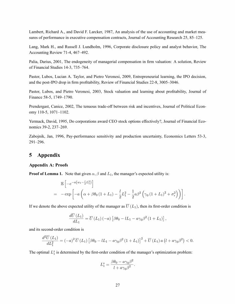
Appendix A: Proofs

Proof of Lemma 1. Note that given �; � and L1, the manager's expected utility is:

Eh�e�a(w1�

l2L21)i

= � exp��a��+ ��0 (1 + L1)�

l

2L21 �

1

2a�2

� 0 (1 + L1)

2 + �2�

���:

If we denote the above expected utility of the manager as U (L1), then its �rst-order condition is

dU (L1)

dL1= U (L1) (�a)

���0 � lL1 � a 0�2 (1 + L1)

�;

and its second-order condition is

d2U (L1)

dL21= (�a)2 U (L1)

���0 � lL1 � a 0�2 (1 + L1)

�2+ U (L1) a

�l + a 0�

2�< 0:

The optimal L�1 is determined by the �rst-order condition of the manager's optimization problem:

L�1 =��0 � a 0�2

l + a 0�2 :

27

The �xed salary � is chosen to satisfy the manager's participation constraint:

�+ ��0 (1 + L�1)�

l

2L�21 �

1

2a�2

� 0 (1 + L

�1)2 + �2�

�= �1

alog��bU� ;

or, after substituting the expression of L�1 and bU = �1, we have� = ���0

l + �0�

l + a 0�2 +

1

2

�2��20 + al 0

�l + a 0�

2 +1

2a�2��

2:

Proof of Proposition 1. We �rst prove that d��

d 0> 0 holds when the manager is risk neutral (i.e., a = 0).

Then the statement in the proposition immediately follows in light of the continuity of the derivatived��=d 0 in a. We can view the maximization problem in terms of implemented effort L�1. If the optimaleffort increases with uncertainty 0:

dL�1d 0

> 0; (10)

and if higher effort is linked to higher incentives, which requires

dL�1d�

> 0; (11)

then we obtain our desired result d��

d 0> 0. Below we proceed to show that both Eq. (10) and Eq. (11)

hold.When a = 0; to implement L�1, the incentive share � satis�es

L�1 =��0l: (12)

Immediately we know that dL�1

d� = �0l > 0, which is just Eq. (11). Now we use supermodularity property

to prove dL�1

d 0> 0. Recall that

V2 (�1) = �1 +(�1 � 1)2

2k+�212k.

Taking expectation, we have

E [V2 (�1)] = �0 +(1� �0)2

2k+�202l+k + l

2kl

� 1 (1 + L

�1)

�2�

�2E ((� � �0) (1 + L�1) + �1)

2

= �0 +(1� �0)2

2k+�202l+k + l

2kl

20 (1 + L�1)2

�2� + 0 (1 + L�1)2 .

Therefore, we can rewrite the principal's objective as (to reduce notation, we use L to denote L�1),

V (L; 0) = E0 (y1 � w1 + V2 (��1))

= �0 (L+ 1)�1

2L2l � 1

2a� 0 (1 + L

�1)2 + �2�

��2

+k + l

2kl

20 (1 + L)2

�2� + 0 (1 + L)2 + �0 +

(1� �0)2

2k+�202l

28

Hence, for a = 0, and ignoring the constant terms, we have

V (L; 0) = �0 (L+ 1)�1

2L2l +

k + l

2kl

20 (1 + L)2

�2� + 0 (1 + L)2 ; (13)

where the �rst term is the �rst period project value, the second term is the effort cost, and the last term isthe second period value. It suf�ces to show that

@2V (L; 0)

@L@ 0> 0:

The �rst two terms are irrelevant. For the last term, notice that (treating (1 + L)2 as a single variable)

k+l2kl @

20(1+L)2

�2�+ 0(1+L)2

@ (L+ 1)2=

k + l

2kl

264 20�2� + 0 (L+ 1)

2 � 30 (L+ 1)

2��2� + 0 (L+ 1)

2�2375

=k + l

2kl

�2���2� 0+ (L+ 1)2

�2 ;which is increasing in 0. Thus,

@2V (L; 0)@L@ 0

> 0. Therefore, we have proven dL�1

d 0> 0, and hence d�

�

d 0> 0

for a = 0. Invoking conitnuity argument, we conclude that our result holds when a is suf�ciently small.

Appendix B: De�nition of Variables

Firm Level Variables

Firm age: Based on Pastor and Veronesi (2003), we consider each �rm as �born� in the year of its �rstappearance in the CRSP database. Speci�cally, we look for the �rst occurrence of a valid stock price onCRSP, as well as the �rst occurrence of a valid market value in the CRSP / COMPUSTAT database, andtake the earlier of the two. The �rm's plain age is assigned the value of one in the year in which the �rmis born and increases by one in each subsequent year. We use natural log of �rm's plain age as the proxyfor uncertainty.

Earnings response coef�cient (ERC): This variable is the ERC1 as de�ned in Pastor, et al. (2009)and is equal to the average of the �rm's previous 12 stock price reactions to quarterly earnings surprises.Speci�cally, we �rst obtain RC, which is the abnormal return due to a quarterly earnings announcementdivided by the unexpected quarterly earnings. The abnormal return is measured as the cumulative return ofstock i in excess of stock i's industry's return starting one trading day before the �rm's earnings announce-ment and ending one trading day after the same announcement. Quarterly earnings announcement datesare from IBES. The industry returns are the daily returns of 49 value-weighted industry portfolios fromKen French's website. The unexpected quarterly earnings are equal to the difference between the actualquarterly earnings per share (obtained from the IBES unadjusted actuals �le) and the mean of all analystforecasts of EPS using IBES's last preannouncement set of forecasts for the given �scal quater, de�ated bybook equity per share of the company. We winsorize RC at 5% and 95% and average the winsorized quar-terly RCs over the rolling three year window to obtain ERC1. Pastor et al. (2009) contain more detailedinformation on constructing the ERC variables.

29

Market to book: (Market value of equity plus the book value of debt)/total assets = (CSHO�PRCC_F+ AT - CEQ)/AT = (data25�data199+data6-data60)/data6.

Tangibility: Net property, plant, and equipment/total assets = PPENT/AT = data8/data6.

Analyst forecast error: For each individual company in each �scal year, we �rst obtain the absolutevalue of the forecast error (equal to the difference between the forecast and the actual EPS values) madeby each analyst, and then we use the median value of these absolute forecast errors scaled by the absolutevalue of the actual EPS. Using the mean value of the absolute forecast errors or scaling by stock priceper share gives similar results. The analyst forecast error variable is constructed from the I/B/E/S detailsdatabase.

Stock return volatility: First obtain the standard deviation of daily log returns over the past �ve years,and then annualize the standard deviation by multiplying by the square root of 254. This is the percentagereturn volatility.

Rank of dollar return volatility: Dollar return volatility is equal to stock percentage return volatilitymultiplied by the beginning-of-year �rm market value. This variable is measured in $millions. Consistentwith Aggarwal and Samwick (1999) and Jin (2002), we employ the percentage ranks of dollar returnvariance in our tests and these percentage ranks range from 0 (lowest risk) to 100 (highest risk).

Investment volatility: This variable is the standard deviation of �rm investment over the past 20 quar-ters, where �rm investment is It=Kt�1, that is, it is equal to capital expenditure in each quarter scaled byprevious quarter-end net property, plant, and equipment (PPENTQ).

Firm size: Natural log of total assets = log(AT) = log(data6). Assets are measured in $millions.

Pro�tability: Operating income before depreciation and amortization/total assets = OIBDP/AT = data13/data6.

Capital expenditure: Capital expenditures/total assets = CAPX/AT = data128/data6.

Advertisement: Advertising expense/total assets = XAD/AT = data45/data6. This variable is set tozero if it is missing and an advertisement missing indicator is thus included in the regressions to deal withthe missing advertisement issue.

Advertisement missing indicator: A dummy variable equal to one if the advertisement variable ismissing.

Leverage: (Long term debt + debt in current liabilities)/total assets = (DLTT+DLC)/AT = (data9+data34)/data6.

Dividend-paying indicator: A dummy variable equal to one if dividends on common stock (data21 orDVC) are strictly positive, and zero otherwise.

CEO chair indicator: A dummy variable equal to one if the CEO of the company is also the boardchairman, and zero otherwise.

Fraction of inside directors: Number of inside board directors divided by board size, where an insidedirector is de�ned as a director who is current or former �rm managers or their family members.

30

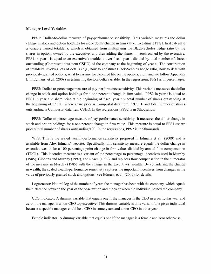
Manager Level Variables

PPS1: Dollar-to-dollar measure of pay-performance sensitivity. This variable measures the dollarchange in stock and option holdings for a one dollar change in �rm value. To estimate PPS1, �rst calculatea variable named totaldelta, which is obtained from multiplying the Black-Scholes hedge ratio by theshares in options owned by the executive, and then adding the shares in stock owned by the executive.PPS1 in year t is equal to an executive's totaldelta over �scal year t divided by total number of sharesoutstanding (Compustat data item CSHO) of the company at the beginning of year t. The constructionof totaldelta involves lots of details (e.g., how to construct Black-Scholes hedge ratio, how to deal withpreviously granted options, what to assume for expected life on the options, etc.), and we follow AppendixB in Edmans, et al. (2009) in estimating the totaldelta variable. In the regressions, PPS1 is in percentages.

PPS2: Dollar-to-percentage measure of pay-performance sensitivity. This variable measures the dollarchange in stock and option holdings for a one percent change in �rm value. PPS2 in year t is equal toPPS1 in year t � share price at the beginning of �scal year t � total number of shares outstanding atthe beginning of t / 100, where share price is Compustat data item PRCC_F and total number of sharesoutstanding is Compustat data item CSHO. In the regressions, PPS2 is in $thousands.

PPS2: Dollar-to-percentage measure of pay-performance sensitivity. It measures the dollar change instock and option holdings for a one percent change in �rm value. This measure is equal to PPS1�shareprice�total number of shares outstanding/100. In the regressions, PPS2 is in $thousands.

WPS: This is the scaled wealth-performance sensitivity proposed in Edmans et al. (2009) and isavailable from Alex Edmans' website. Speci�cally, this sensitivity measure equals the dollar change inexecutive wealth for a 100 percentage point change in �rm value, divided by annual �ow compensation(TDC1). This incentive measure is a variant of the percentage-to-percentage incentives used in Murphy(1985), Gibbons and Murphy (1992), and Rosen (1992), and replaces �ow compensation in the numeratorof the measure in Murphy (1985) with the change in the executives' wealth. By considering the changein wealth, the scaled wealth-performance sensitivity captures the important incentives from changes in thevalue of previously granted stock and options. See Edmans et al. (2009) for details.

Log(tenure): Natural log of the number of years the manager has been with the company, which equalsthe difference between the year of the observation and the year when the individual joined the company.

CEO indicator: A dummy variable that equals one if the manager is the CEO in a particular year andzero if the manager is a non-CEO top executive. This dummy variable is time variant for a given individualbecause a speci�c manager could be a CEO in some years and a non-CEO in other years.

Female indicator: A dummy variable that equals one if the manager is a female and zero otherwise.

31

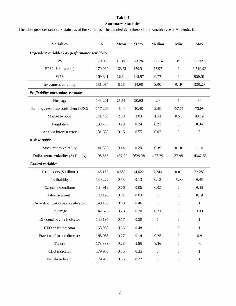
32

Table 1 Summary Statistics

The table provides summary statistics of the variables. The detailed definitions of the variables are in Appendix B.

Variables N Mean Stdev Median Min Max

Dependent variable: Pay-performance sensitivity

PPS1 179,930 1.13% 3.15% 0.22% 0% 22.66%

PPS2 ($thousands) 179,930 168.61 476.91 27.97 0 3,519.93

WPS 169,841 36.34 119.97 6.77 0 939.61

Investment volatility 151,954 6.05 14.00 3.00 0.19 336.20

Profitability uncertainty variables

Firm age 143,291 25.56 20.02 20 1 84

Earnings response coefficient (ERC) 117,263 4.44 10.40 2.88 -57.01 75.09

Market to book 141,405 2.08 2.03 1.51 0.51 43.19

Tangibility 139,799 0.29 0.24 0.23 0 0.94

Analyst forecast error 131,689 0.16 0.55 0.03 0 6

Risk variable

Stock return volatility 141,623 0.44 0.20 0.39 0.18 1.14

Dollar return volatility ($millions) 108,557 1497.20 2639.38 477.79 27.98 14382.63

Control variables

Total assets ($millions) 143,182 6,589 14,022 1,343 0.07 72,282

Profitability 140,222 0.13 0.13 0.13 -5.09 0.45

Capital expenditure 134,919 0.06 0.06 0.05 0 0.48

Advertisement 143,195 0.01 0.03 0 0 0.19

Advertisement missing indicator 143,195 0.69 0.46 1 0 1

Leverage 142,528 0.23 0.20 0.21 0 3.09

Dividend paying indicator 143,195 0.57 0.50 1 0 1

CEO chair indicator 163,936 0.65 0.48 1 0 1

Fraction of inside directors 163,936 0.27 0.14 0.25 0 0.9

Tenure 173,383 9.23 5.85 8.86 0 40

CEO indicator 179,930 0.15 0.35 0 0 1

Female indicator 179,930 0.05 0.22 0 0 1

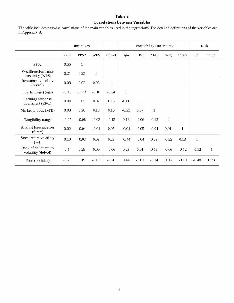
33

Table 2 Correlations between Variables

The table includes pairwise correlations of the main variables used in the regressions. The detailed definitions of the variables are in Appendix B.

Incentives Profitability Uncertainty Risk

PPS1 PPS2 WPS invvol age ERC M/B tang forerr vol dolvol

PPS2 0.55 1

Wealth-performance sensitivity (WPS) 0.21 0.25 1

Investment volatility (invvol) 0.08 0.02 0.05 1

Log(firm age) (age) -0.16 0.003 -0.10 -0.24 1

Earnings response coefficient (ERC) 0.04 0.05 0.07 0.007 -0.06 1

Market to book (M/B) 0.08 0.20 0.19 0.16 -0.23 0.07 1

Tangibility (tang) -0.05 -0.08 -0.03 -0.15 0.18 -0.06 -0.12 1

Analyst forecast error (forerr)

0.02 -0.04 -0.01 0.05 -0.04 -0.05 -0.04 0.01 1

Stock return volatility (vol)

0.10 -0.03 0.03 0.28 -0.44 -0.04 0.23 -0.22 0.13 1

Rank of dollar return volatility (dolvol)

-0.14 0.29 0.09 -0.06 0.23 0.01 0.16 -0.06 -0.12 -0.12 1

Firm size (size) -0.20 0.19 -0.03 -0.20 0.44 -0.01 -0.24 0.03 -0.10 -0.48 0.73

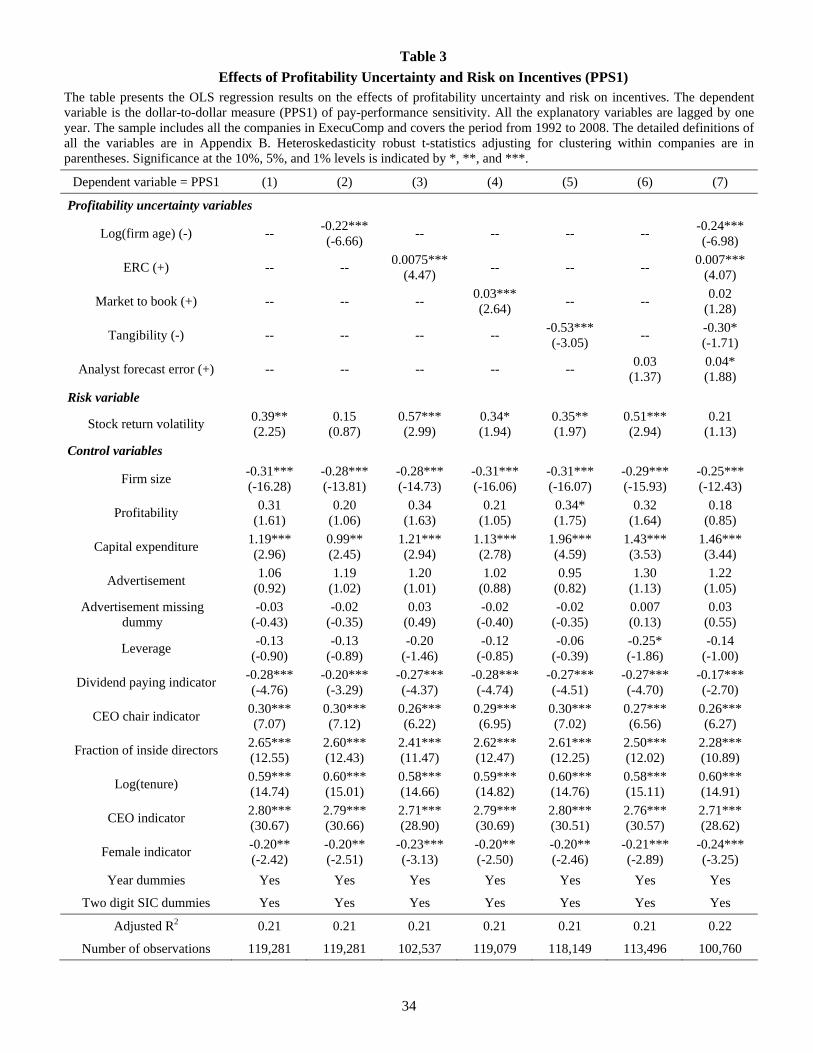
34

Table 3 Effects of Profitability Uncertainty and Risk on Incentives (PPS1)

The table presents the OLS regression results on the effects of profitability uncertainty and risk on incentives. The dependent variable is the dollar-to-dollar measure (PPS1) of pay-performance sensitivity. All the explanatory variables are lagged by one year. The sample includes all the companies in ExecuComp and covers the period from 1992 to 2008. The detailed definitions of all the variables are in Appendix B. Heteroskedasticity robust t-statistics adjusting for clustering within companies are in parentheses. Significance at the 10%, 5%, and 1% levels is indicated by *, **, and ***.

Dependent variable = PPS1 (1) (2) (3) (4) (5) (6) (7)

Profitability uncertainty variables

Log(firm age) (-) -- -0.22*** (-6.66) -- -- -- -- -0.24***

(-6.98)

ERC (+) -- -- 0.0075*** (4.47) -- -- -- 0.007***

(4.07)

Market to book (+) -- -- -- 0.03*** (2.64) -- -- 0.02

(1.28)

Tangibility (-) -- -- -- -- -0.53*** (-3.05) -- -0.30*

(-1.71)

Analyst forecast error (+) -- -- -- -- -- 0.03 (1.37)

0.04* (1.88)

Risk variable

Stock return volatility 0.39** (2.25)

0.15 (0.87)

0.57*** (2.99)

0.34* (1.94)

0.35** (1.97)

0.51*** (2.94)

0.21 (1.13)

Control variables

Firm size -0.31*** (-16.28)

-0.28*** (-13.81)

-0.28*** (-14.73)

-0.31*** (-16.06)

-0.31*** (-16.07)

-0.29*** (-15.93)

-0.25*** (-12.43)

Profitability 0.31 (1.61)

0.20 (1.06)

0.34 (1.63)

0.21 (1.05)

0.34* (1.75)

0.32 (1.64)

0.18 (0.85)

Capital expenditure 1.19*** (2.96)

0.99** (2.45)

1.21*** (2.94)

1.13*** (2.78)

1.96*** (4.59)

1.43*** (3.53)

1.46*** (3.44)

Advertisement 1.06 (0.92)

1.19 (1.02)

1.20 (1.01)

1.02 (0.88)

0.95 (0.82)

1.30 (1.13)

1.22 (1.05)

Advertisement missing dummy

-0.03 (-0.43)

-0.02 (-0.35)

0.03 (0.49)

-0.02 (-0.40)

-0.02 (-0.35)

0.007 (0.13)

0.03 (0.55)

Leverage -0.13 (-0.90)

-0.13 (-0.89)

-0.20 (-1.46)

-0.12 (-0.85)

-0.06 (-0.39)

-0.25* (-1.86)

-0.14 (-1.00)

Dividend paying indicator -0.28*** (-4.76)

-0.20*** (-3.29)

-0.27*** (-4.37)

-0.28*** (-4.74)

-0.27*** (-4.51)

-0.27*** (-4.70)

-0.17*** (-2.70)

CEO chair indicator 0.30*** (7.07)

0.30*** (7.12)

0.26*** (6.22)

0.29*** (6.95)

0.30*** (7.02)

0.27*** (6.56)

0.26*** (6.27)

Fraction of inside directors 2.65*** (12.55)

2.60*** (12.43)

2.41*** (11.47)

2.62*** (12.47)

2.61*** (12.25)

2.50*** (12.02)

2.28*** (10.89)

Log(tenure) 0.59*** (14.74)

0.60*** (15.01)

0.58*** (14.66)

0.59*** (14.82)

0.60*** (14.76)

0.58*** (15.11)

0.60*** (14.91)

CEO indicator 2.80*** (30.67)

2.79*** (30.66)

2.71*** (28.90)

2.79*** (30.69)

2.80*** (30.51)

2.76*** (30.57)

2.71*** (28.62)

Female indicator -0.20** (-2.42)

-0.20** (-2.51)

-0.23*** (-3.13)

-0.20** (-2.50)

-0.20** (-2.46)

-0.21*** (-2.89)

-0.24*** (-3.25)

Year dummies Yes Yes Yes Yes Yes Yes Yes

Two digit SIC dummies Yes Yes Yes Yes Yes Yes Yes

Adjusted R2 0.21 0.21 0.21 0.21 0.21 0.21 0.22

Number of observations 119,281 119,281 102,537 119,079 118,149 113,496 100,760

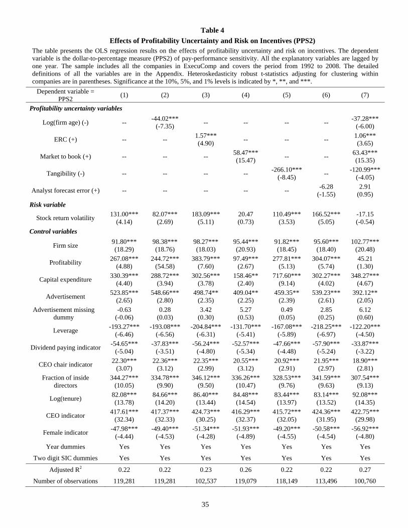
35

Table 4 Effects of Profitability Uncertainty and Risk on Incentives (PPS2)

The table presents the OLS regression results on the effects of profitability uncertainty and risk on incentives. The dependent variable is the dollar-to-percentage measure (PPS2) of pay-performance sensitivity. All the explanatory variables are lagged by one year. The sample includes all the companies in ExecuComp and covers the period from 1992 to 2008. The detailed definitions of all the variables are in the Appendix. Heteroskedasticity robust t-statistics adjusting for clustering within companies are in parentheses. Significance at the 10%, 5%, and 1% levels is indicated by *, **, and ***.

Dependent variable = PPS2 (1) (2) (3) (4) (5) (6) (7)

Profitability uncertainty variables

Log(firm age) (-) -- -44.02*** (-7.35) -- -- -- -- -37.28***

(-6.00)

ERC (+) -- -- 1.57*** (4.90) -- -- -- 1.06***

(3.65)

Market to book (+) -- -- -- 58.47*** (15.47) -- -- 63.43***

(15.35)

Tangibility (-) -- -- -- -- -266.10*** (-8.45) -- -120.99***

(-4.05)

Analyst forecast error (+) -- -- -- -- -- -6.28 (-1.55)

2.91 (0.95)

Risk variable

Stock return volatility 131.00*** (4.14)

82.07*** (2.69)

183.09*** (5.11)

20.47 (0.73)

110.49*** (3.53)

166.52*** (5.05)

-17.15 (-0.54)

Control variables

Firm size 91.80*** (18.29)

98.38*** (18.76)

98.27*** (18.03)

95.44*** (20.93)

91.82*** (18.45)

95.60*** (18.40)

102.77*** (20.48)

Profitability 267.08*** (4.88)

244.72*** (54.58)

383.79*** (7.60)

97.49*** (2.67)

277.81*** (5.13)

304.07*** (5.74)

45.21 (1.30)

Capital expenditure 330.39*** (4.40)

288.72*** (3.94)

302.56*** (3.78)

158.46** (2.40)

717.60*** (9.14)

302.27*** (4.02)

348.27*** (4.67)

Advertisement 523.85*** (2.65)

548.66*** (2.80)

498.74** (2.35)

409.04** (2.25)

459.35** (2.39)

539.23*** (2.61)

392.12** (2.05)

Advertisement missing dummy

-0.63 (-0.06)

0.28 (0.03)

3.42 (0.30)

5.27 (0.53)

0.49 (0.05)

2.85 (0.25)

6.12 (0.60)

Leverage -193.27*** (-6.46)

-193.08*** (-6.56)

-204.84*** (-6.31)

-131.70*** (-5.41)

-167.08*** (-5.89)

-218.25*** (-6.97)

-122.20*** (-4.50)

Dividend paying indicator -54.65*** (-5.04)

-37.83*** (-3.51)

-56.24*** (-4.80)

-52.57*** (-5.34)

-47.66*** (-4.48)

-57.90*** (-5.24)

-33.87*** (-3.22)

CEO chair indicator 22.30*** (3.07)

22.36*** (3.12)

22.35*** (2.99)

20.55*** (3.12)

20.92*** (2.91)

21.95*** (2.97)

18.90*** (2.81)

Fraction of inside directors

344.27*** (10.05)

334.78*** (9.90)

346.12*** (9.50)

336.26*** (10.47)

328.53*** (9.76)

341.59*** (9.63)

307.54*** (9.13)

Log(tenure) 82.08*** (13.78)

84.66*** (14.20)

86.40*** (13.44)

84.48*** (14.54)

83.44*** (13.97)

83.14*** (13.52)

92.08*** (14.35)

CEO indicator 417.61*** (32.34)

417.37*** (32.33)

424.73*** (30.25)

416.29*** (32.37)

415.72*** (32.05)

424.36*** (31.95)

422.75*** (29.98)

Female indicator -47.98*** (-4.44)

-49.40*** (-4.53)

-51.34*** (-4.28)

-51.93*** (-4.89)

-49.20*** (-4.55)

-50.58*** (-4.54)

-56.92*** (-4.80)

Year dummies Yes Yes Yes Yes Yes Yes Yes

Two digit SIC dummies Yes Yes Yes Yes Yes Yes Yes

Adjusted R2 0.22 0.22 0.23 0.26 0.22 0.22 0.27

Number of observations 119,281 119,281 102,537 119,079 118,149 113,496 100,760

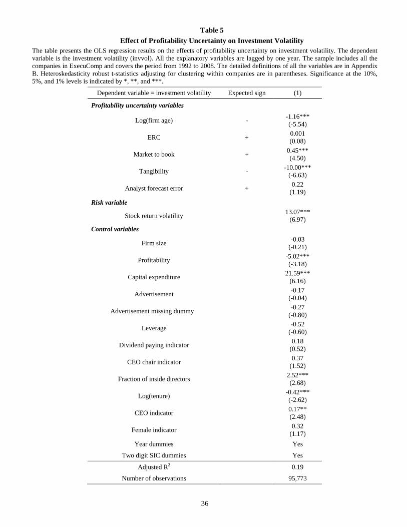
36

Table 5 Effect of Profitability Uncertainty on Investment Volatility

The table presents the OLS regression results on the effects of profitability uncertainty on investment volatility. The dependent variable is the investment volatility (invvol). All the explanatory variables are lagged by one year. The sample includes all the companies in ExecuComp and covers the period from 1992 to 2008. The detailed definitions of all the variables are in Appendix B. Heteroskedasticity robust t-statistics adjusting for clustering within companies are in parentheses. Significance at the 10%, 5%, and 1% levels is indicated by *, **, and ***.

Dependent variable = investment volatility Expected sign (1)

Profitability uncertainty variables

Log(firm age) - -1.16*** (-5.54)

ERC + 0.001 (0.08)

Market to book + 0.45*** (4.50)

Tangibility - -10.00*** (-6.63)

Analyst forecast error + 0.22 (1.19)

Risk variable

Stock return volatility 13.07*** (6.97)

Control variables

Firm size -0.03 (-0.21)

Profitability -5.02*** (-3.18)

Capital expenditure 21.59*** (6.16)

Advertisement -0.17 (-0.04)

Advertisement missing dummy -0.27 (-0.80)

Leverage -0.52 (-0.60)

Dividend paying indicator 0.18 (0.52)

CEO chair indicator 0.37 (1.52)

Fraction of inside directors 2.52*** (2.68)

Log(tenure) -0.42*** (-2.62)

CEO indicator 0.17** (2.48)

Female indicator 0.32 (1.17)

Year dummies Yes

Two digit SIC dummies Yes

Adjusted R2 0.19

Number of observations 95,773

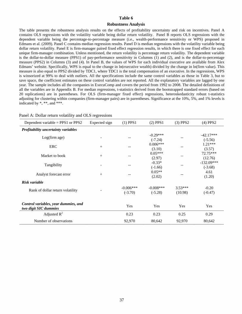
37

Table 6 Robustness Analysis

The table presents the robustness analysis results on the effects of profitability uncertainty and risk on incentives. Panel A contains OLS regressions with the volatility variable being dollar return volatility. Panel B reports OLS regressions with the dependent variable being the percentage-to-percentage measure (i.e., wealth-performance sensitivity or WPS) proposed in Edmans et al. (2009). Panel C contains median regression results. Panel D is median regressions with the volatility variable being dollar return volatility. Panel E is firm-manager paired fixed effect regression results, in which there is one fixed effect for each unique firm-manager combination. Unless mentioned, the return volatility is percentage return volatility. The dependent variable is the dollar-to-dollar measure (PPS1) of pay-performance sensitivity in Columns (1) and (2), and is the dollar-to-percentage measure (PPS2) in Columns (3) and (4). In Panel B, the values of WPS for each individual executive are available from Alex Edmans’ website. Specifically, WPS is equal to the change in ln(executive wealth) divided by the change in ln(firm value). This measure is also equal to PPS2 divided by TDC1, where TDC1 is the total compensation of an executive. In the regressions, WPS is winsorized at 99% to deal with outliers. All the specifications include the same control variables as those in Table 3, but to save space, the coefficient estimates on these control variables are not reported. All the explanatory variables are lagged by one year. The sample includes all the companies in ExecuComp and covers the period from 1992 to 2008. The detailed definitions of all the variables are in Appendix B. For median regressions, t-statistics derived from the bootstrapped standard errors (based on 20 replications) are in parentheses. For OLS (firm-manager fixed effect) regressions, heteroskedasticity robust t-statistics adjusting for clustering within companies (firm-manager pairs) are in parentheses. Significance at the 10%, 5%, and 1% levels is indicated by *, **, and ***. Panel A: Dollar return volatility and OLS regressions

Dependent variable = PPS1 or PPS2 Expected sign (1) PPS1 (2) PPS1 (3) PPS2 (4) PPS2

Profitability uncertainty variables

Log(firm age) - -- -0.29*** (-7.24) -- -42.17***

(-5.56)

ERC + -- 0.006*** (3.10) -- 1.21***

(3.57)

Market to book + -- 0.05*** (2.97) -- 72.75***

(12.76)

Tangibility - -- -0.33* (-1.66) -- -132.09***

(-3.68)

Analyst forecast error + -- 0.05** (2.02) -- 4.61

(1.20) Risk variable

Rank of dollar return volatility - -0.006*** (-3.70)

-0.008*** (-5.28)

3.53*** (10.98)

-0.20 (-0.47)

Control variables, year dummies, and two digit SIC dummies Yes Yes Yes Yes

Adjusted R2 0.23 0.23 0.25 0.29

Number of observations 92,970 80,642 92,970 80,642

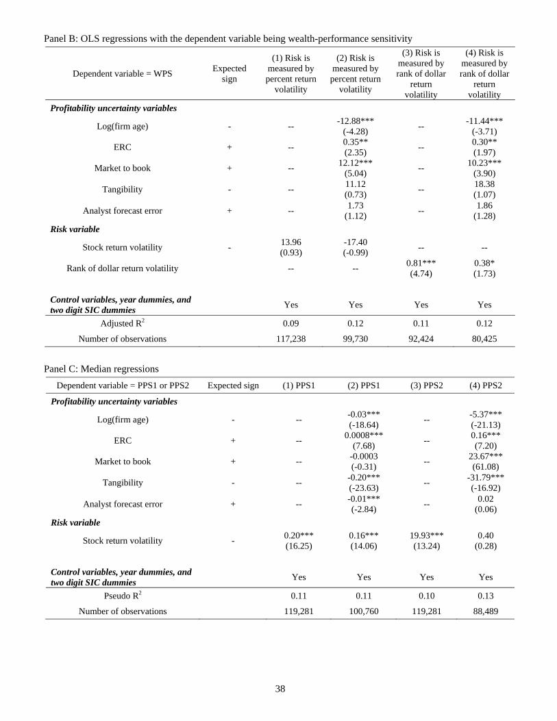
38

Panel B: OLS regressions with the dependent variable being wealth-performance sensitivity

Dependent variable = WPS Expected sign

(1) Risk is measured by percent return

volatility

(2) Risk is measured by

percent return volatility

(3) Risk is measured by rank of dollar

return volatility

(4) Risk is measured by rank of dollar

return volatility

Profitability uncertainty variables

Log(firm age) - -- -12.88*** (-4.28) -- -11.44***

(-3.71)

ERC + -- 0.35** (2.35) -- 0.30**

(1.97)

Market to book + -- 12.12*** (5.04) -- 10.23***

(3.90)

Tangibility - -- 11.12 (0.73) -- 18.38

(1.07)

Analyst forecast error + -- 1.73 (1.12) -- 1.86

(1.28) Risk variable

Stock return volatility - 13.96 (0.93)

-17.40 (-0.99) -- --

Rank of dollar return volatility -- -- 0.81*** (4.74)

0.38* (1.73)

Control variables, year dummies, and two digit SIC dummies Yes Yes Yes Yes

Adjusted R2 0.09 0.12 0.11 0.12

Number of observations 117,238 99,730 92,424 80,425

Panel C: Median regressions

Dependent variable = PPS1 or PPS2 Expected sign (1) PPS1 (2) PPS1 (3) PPS2 (4) PPS2

Profitability uncertainty variables

Log(firm age) - -- -0.03*** (-18.64) -- -5.37***

(-21.13)

ERC + -- 0.0008*** (7.68) -- 0.16***

(7.20)

Market to book + -- -0.0003 (-0.31) -- 23.67***

(61.08)

Tangibility - -- -0.20*** (-23.63) -- -31.79***

(-16.92)

Analyst forecast error + -- -0.01*** (-2.84) -- 0.02

(0.06) Risk variable

Stock return volatility - 0.20*** (16.25)

0.16*** (14.06)

19.93*** (13.24)

0.40 (0.28)

Control variables, year dummies, and two digit SIC dummies Yes Yes Yes Yes

Pseudo R2 0.11 0.11 0.10 0.13

Number of observations 119,281 100,760 119,281 88,489

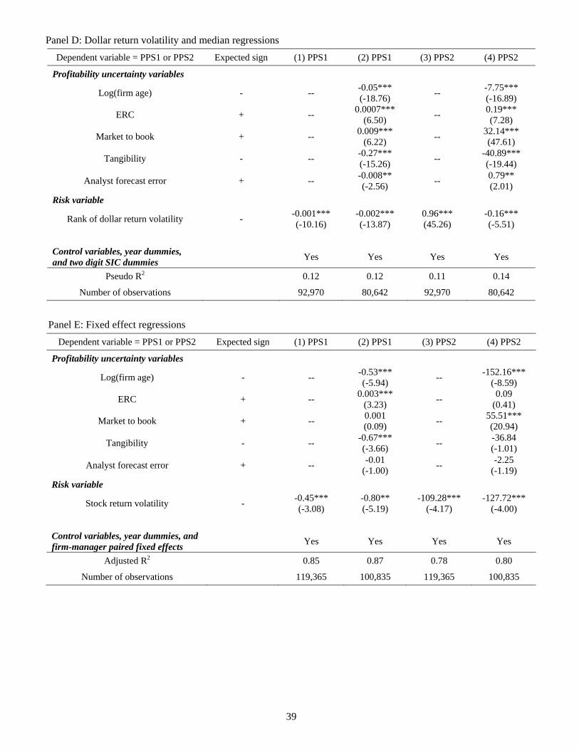
39

Panel D: Dollar return volatility and median regressions Dependent variable = PPS1 or PPS2 Expected sign (1) PPS1 (2) PPS1 (3) PPS2 (4) PPS2

Profitability uncertainty variables

Log(firm age) - -- -0.05*** (-18.76) -- -7.75***

(-16.89)

ERC + -- 0.0007*** (6.50) -- 0.19***

(7.28)

Market to book + -- 0.009*** (6.22) -- 32.14***

(47.61)

Tangibility - -- -0.27*** (-15.26) -- -40.89***

(-19.44)

Analyst forecast error + -- -0.008** (-2.56) -- 0.79**

(2.01) Risk variable

Rank of dollar return volatility - -0.001*** (-10.16)

-0.002*** (-13.87)

0.96*** (45.26)

-0.16*** (-5.51)

Control variables, year dummies, and two digit SIC dummies Yes Yes Yes Yes

Pseudo R2 0.12 0.12 0.11 0.14

Number of observations 92,970 80,642 92,970 80,642

Panel E: Fixed effect regressions

Dependent variable = PPS1 or PPS2 Expected sign (1) PPS1 (2) PPS1 (3) PPS2 (4) PPS2

Profitability uncertainty variables

Log(firm age) - -- -0.53*** (-5.94) -- -152.16***

(-8.59)

ERC + -- 0.003*** (3.23) -- 0.09

(0.41)

Market to book + -- 0.001 (0.09) -- 55.51***

(20.94)

Tangibility - -- -0.67*** (-3.66) -- -36.84

(-1.01)

Analyst forecast error + -- -0.01 (-1.00) -- -2.25

(-1.19) Risk variable

Stock return volatility - -0.45*** (-3.08)

-0.80** (-5.19)

-109.28*** (-4.17)

-127.72*** (-4.00)

Control variables, year dummies, and firm-manager paired fixed effects Yes Yes Yes Yes

Adjusted R2 0.85 0.87 0.78 0.80

Number of observations 119,365 100,835 119,365 100,835