iCT Conference 2014 – www.3dct.at 189

Uncertainty in CT Metrology: Visualizations for Exploration and Analysis of Geometric Tolerances

Artem Amirkhanov1, Bernhard Fröhler1, Michael Reiter1, Johann Kastner1, M. Eduard Grӧller2, Christoph Heinzl1

1Upper Austrian University of Applied Sciences, Wels Campus, Austria, e-mail: Artem.Amirkhanov@fh-wels.at, Christoph.Heinzl@fh-wels.at,

Michael.Reiter@fh-wels.at, Johann.Kastner@fh-wels.at 2Institute of Computer Graphics and Algorithms, Vienna University of Technology,

Vienna, Austria, e-mail: groeller@cg.tuwien.ac.at

Abstract Industrial 3D X-ray computed tomography (3DXCT) is increasingly applied as a technique for metrology applications. In contrast to comventional metrology tools such as coordinate measurement machines (CMMs). 3DXCT only estimates the exact position of the specimen’s surface and is subjected to a specific set of artifact types. These factors result in uncertainty that is present in the data. Previous work by Amirkhanov et. al [2] presented a tool prototype that is taking such uncertainty into account when measuring geometric tolerances such as straightness, circularity, or flatness. In this paper we extend the previous work with two more geometric tolerance types: cylindricity and angularity. We provide methods and tools for visualization, inspection, and analysis of these tolerances. For the cylindricity tolerance we employ neighboring profiles visualization, box-plot overview, and interactive 3D view. We evaluate applicability and usefulness our methods on a new TP03 data set, and present results and new potential use cases.

Keywords: Industrial 3D computed tomography, uncertainty visualization, level-of-details, metrology

1 Introduction Metrology through geometric dimensioning and tolerancing is one of the most important and widely applied methodologies for non-destructive testing and quality control in industrial manufacturing. Typically the measurement procedure is performed using specialized tactile or optical coordinate measurement machines (CMMs). CMMs evaluate tolerances for the set of defined dimensional measurment features by directly evaluating the surface of the specimen. In recent years, industrial 3D X-ray computed tomography (3DXCT) has been getting increasingly more popular for metrology applications. Since 3DXCT systems with higher accuracy are developed, the choice of 3DXCT is often motivated by their ability to capture both internal and external structures of a specimen within one scan. However, to perform dimensional measurements, one more step has to be performed comparing to CMMs. Using 3DXCT volumetric data, the location of the specimen surface has to be estimated based on the scanned attenuation coefficients. As opposed to tactile or optical measurement techniques, the surface is not explicit and implies a particular positional uncertainty depending on discretization, artifacts and noise in the scan data and the used surface extraction algorithm. Currently, to our knowledge, there are no 3DXCT metrology software systems available that completely account for these uncertainties and consider them when presenting measurement results.

190

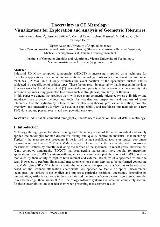
Figure 1: Workflow of 3DXCT dimensional metrology accounting for measurement uncertainty.

In [2] we presented a tool that estimates positional uncertainties of the extracted specimen’s surface and utilizes this information in a set of visualizations on various levels-of-detail. These visualizations are combined in one integrated software tool utilizing linked views, 3D tolerance tagging, and measurement profile plotting functionalities. The workflow of the tool is shown in Figure 1. Geometric tolerance indications are provided as smart tolerance tags. The underlying uncertainty of the specimen surface is visualized as context in measurement plots commonly used and familiar to the metrology experts. The proposed visualizations serve the goal of providing an augmented insight into the reliability of geometric tolerances as they are affected by various factors and errors during 3DXCT scanning and reconstruction. On the other hand, we intend to maintain the daily workflow of domain specialists but enhance it by showing more information on the nature of highly uncertain regions. The tolerances presented in [2] were primarily straightness and circularity. In this work we further extend applications of the uncertainty visualization techniques on 3D geometric tolerances, such as cylindricity and angularity. We present new visualizations providing an overview about the overall quality and uncertainty level of the entire tolerance. This provides the user with ability to estimate deviations and uncertainty distributions along the measurement profile of 3D primitive. An easy

iCT Conference 2014 – www.3dct.at 191

navigation to the regions of interest is then possible for a more detailed exploration. Another contribution of this work is a detailed evaluation of the presented techniques. An extended evaluation is performed using new 3DXCT scans and is presented with more use cases. In summary, this work contains the following contributions which set it apart from the previous work [2]:

New types of geometric tolerances that can take into account intersection probability: cylindricity and angularity.

A set of visualizations providing overview and allowing for exploration and analysis of 3D tolerance data: box-plot cylindricity overview plot, linked 2D and 3D cylindricity views, visualizing single probing profile of the cylindricity in context of the neighboring probing circles.

Application of the presented methods to a new dataset and extended evaluation with additional use cases.

2 Dataset

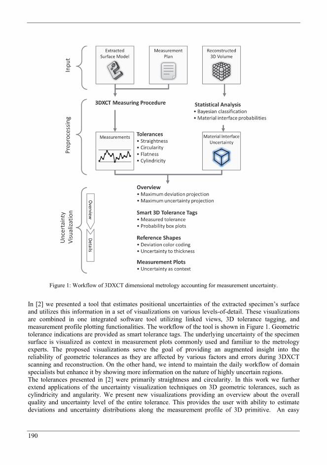
Figure 2: The 2D slice of 3DXCT scan (top) and the engineering drawing of the TP03 specimen in three

projections (bottom).

We evaluate our methods using the TP03 dataset (see Figure2). It is a test phantom made of aluminium: the lower part has a shape of conoid, has four smaller drill holes at the bottom and one bigger drill hole on the side; the upper part is a cylinder with two drill holes on the top and one drill hole on the side; one big drill hole going through the entire specimen from the top to the bottom. During the scanning the specimen was tilted to the angle of 15 degrees to avoid the blurring of top and bottom faces. We used the 3D volume scan to compute an intersection probability volume [2]. The iso surface used for measurements was extracted using the value of 41500 which is corresponding to the intersection of the Gaussian curves fitted to the air and alluminium distributions during the Bayesian classification algorithm [3].

192

3 Added Geometric Tolerances We extended the tool [2] with two new types of geometric tolerances which are widely used by the domain experts in the area of metrology: cylindricity (Section 3.1), and angularity (Section 3.2).

3.1 Cylindricity

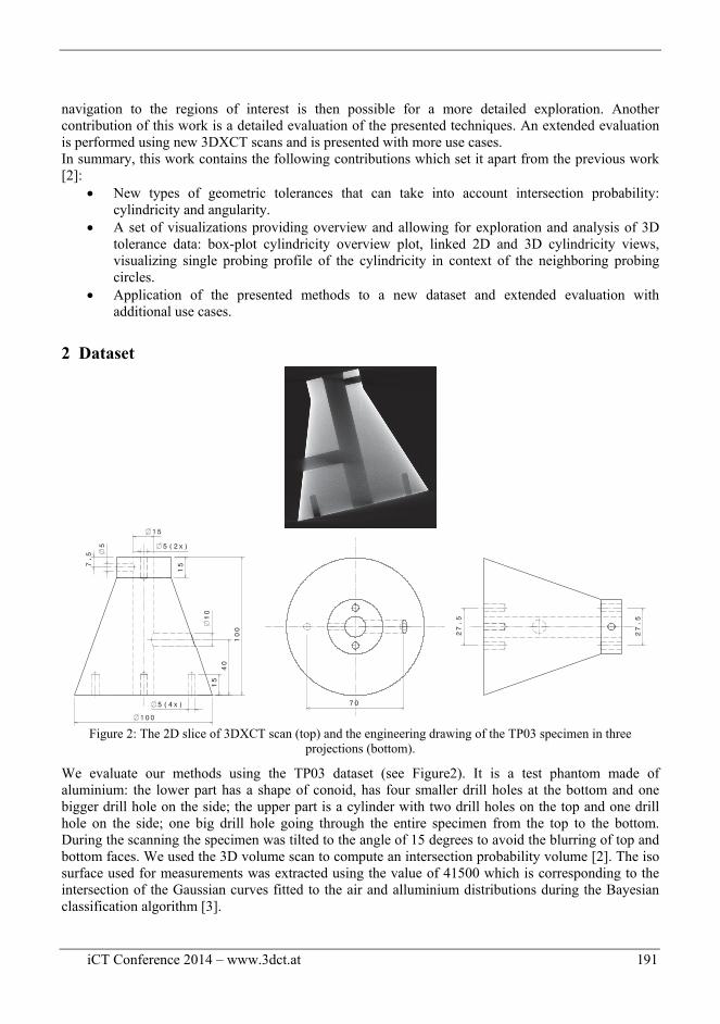
Figure 3: Views used for cylindricity inspection.

For measuring the cylindricity tolerance, we utilize a probing trajectory composed of individual circles. This allows us to use circularity polar plot for the inspection of each probing circle. The GUI for detailed visualization and analysis of the cylindricity tolerance contains three linked views (see Figure 3): polar plot view (a), box-plot overview (b), and interactive 3D view (c). The polar plot view has the same functionality as the circularity polar plot (see [2]) but allows the user to navigate between different probing circles. Additionally, the cylindricity polar plot is capable of visualizing single probing profile in the context of the neighboring probing circles (see Figure 3a). The currently selected profile is shown with black, the neighboring profiles that are coming before the selected one are indicated with red, and profiles coming after are shown with blue. The widths and transparencies of the line indicate how close the profile is to the selected one. Such a representation is designed to assist in visual detection of various patterns in the deviations, e.g., defects, or crookedness of the cylindrical feature. The box plot view provides an overview for the distribution of the measured cylindricity deviations along the length of the cylinder. For each probing circle, all the measured deviations are used to calculate the corresponding box plot parameters: minimum deviation, lower quantile, median deviation, higher quantile, and the maximum deviation. The resulting box plots are then shown in the context of the reference shape and its tolerance zone. Such representation of the cylindricity tolerance allows to estimate the deviations along the measured cylinder in a single glance and to easily detect the problematic areas. The polar plot view can then be utilized for a more detailed inspection. The view linking is implemented in the following way:

The point that is highlighted in the polar plot view is marked with the red arrow marker in the interactive 3D view. When the user hovers a mouse over the polar plot view, the corresponding point is interactively marked;

iCT Conference 2014 – www.3dct.at 193

The red marker in the box plot overview is denoting a box plot corresponding to the probing circle currently shown in the polar plot view. When the user switches to another probing circle, the position of the marker changes and the polar plot view is updated.

3.2 Angular Tolerances

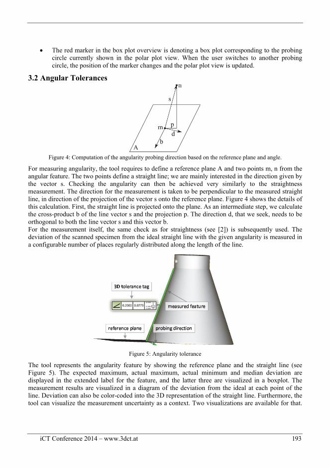
Figure 4: Computation of the angularity probing direction based on the reference plane and angle.

For measuring angularity, the tool requires to define a reference plane A and two points m, n from the angular feature. The two points define a straight line; we are mainly interested in the direction given by the vector s. Checking the angularity can then be achieved very similarly to the straightness measurement. The direction for the measurement is taken to be perpendicular to the measured straight line, in direction of the projection of the vector s onto the reference plane. Figure 4 shows the details of this calculation. First, the straight line is projected onto the plane. As an intermediate step, we calculate the cross-product b of the line vector s and the projection p. The direction d, that we seek, needs to be orthogonal to both the line vector s and this vector b. For the measurement itself, the same check as for straightness (see [2]) is subsequently used. The deviation of the scanned specimen from the ideal straight line with the given angularity is measured in a configurable number of places regularly distributed along the length of the line.

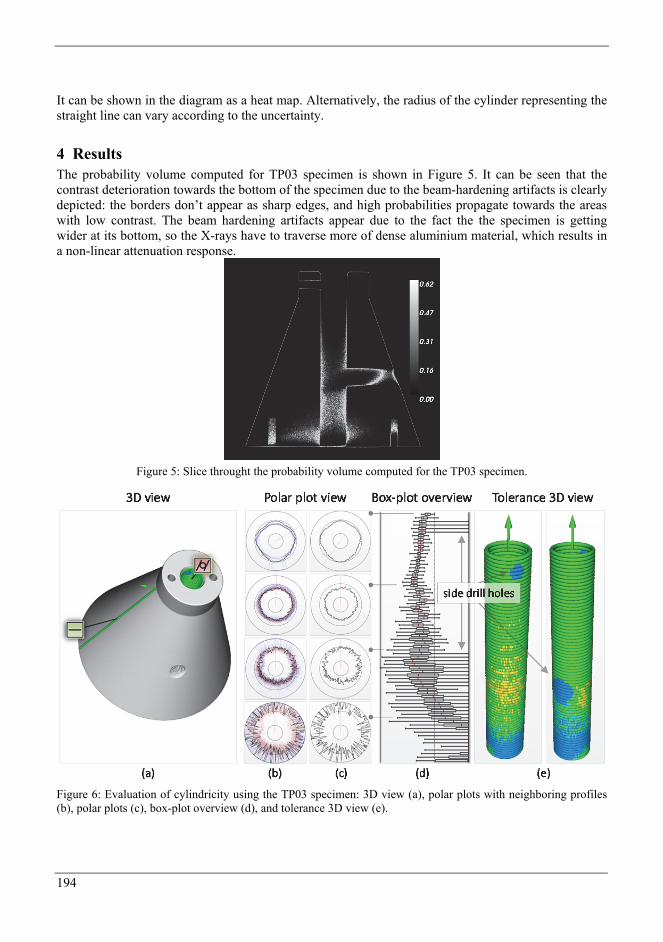
Figure 5: Angularity tolerance

The tool represents the angularity feature by showing the reference plane and the straight line (see Figure 5). The expected maximum, actual maximum, actual minimum and median deviation are displayed in the extended label for the feature, and the latter three are visualized in a boxplot. The measurement results are visualized in a diagram of the deviation from the ideal at each point of the line. Deviation can also be color-coded into the 3D representation of the straight line. Furthermore, the tool can visualize the measurement uncertainty as a context. Two visualizations are available for that.

194

It can be shown in the diagram as a heat map. Alternatively, the radius of the cylinder representing the straight line can vary according to the uncertainty.

4 Results The probability volume computed for TP03 specimen is shown in Figure 5. It can be seen that the contrast deterioration towards the bottom of the specimen due to the beam-hardening artifacts is clearly depicted: the borders don’t appear as sharp edges, and high probabilities propagate towards the areas with low contrast. The beam hardening artifacts appear due to the fact the the specimen is getting wider at its bottom, so the X-rays have to traverse more of dense aluminium material, which results in a non-linear attenuation response.

Figure 5: Slice throught the probability volume computed for the TP03 specimen.

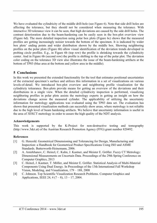
Figure 6: Evaluation of cylindricity using the TP03 specimen: 3D view (a), polar plots with neighboring profiles (b), polar plots (c), box-plot overview (d), and tolerance 3D view (e).

iCT Conference 2014 – www.3dct.at 195

We have evaluated the cylindricity of the middle drill-hole (see Figure 6). Note that side drill holes are affecting the tolerance, but they should not be considered when measuring the tolerance. With interactive 3D tolerance view it can be seen, that high deviations are caused by the side drill holes. The contrast deterioration due to the beam-hardening can be easily seen in the box-plot overview view (Figure 6d). The more detailed inspection using polar box plots (Figure 6c) shows that the measured profiles are getting increasingly noisier towards the bottom of the specimen. It is indicated by wider box plots’ ending points and wider distribution shown by the middle box. Showing neighboring profiles on the polar plots (Figure 6b) allow visual identification of the deviation trends developed in probing circle profiles. E.g., in Figure 6b (top row) the profile is shrinking towards the cylindricity center. And in Figure 6b (second row) the profile is shifting to the top of the polar plot. The deviation color coding on the tolerance 3D view also illustrates the issue of the beam-hardening artifacts at the bottom of TP03 (blue area at the bottom and yellow area in the middle).

5 Conclusions In this work we presented the extended functionality for the tool that estimates positional uncertainties of the extracted specimen’s surface and utilizes this information in a set of visualizations on various levels-of-detail. We introduced box-plot overview and neighboring profile visualization for the cylindricty tolearance. Box-plots provide means for getting an overview of the deviations and their distributions in a single view. When the detailed cylindricity inspection is performed, visualizing neighboring profiles in polar plots assists the metrology experts in getting an insight on how the deviations change across the measured cylinder. The applicability of utilizing the uncertainty information for metrology applications was evaluated using the TP03 data set. The evaluation has shown that presented visualization methods can sucessfuly show areas, where metrology is not reliable due to the high level of beam hardening artifacts. We believe that uncertainty information is useful in the area of 3DXCT metrology in order to assure the high quality of the NDT analysis.

Acknowledgements

This work is supported by the K-Project for non-destructive testing and tomography (http://www.3dct.at) of the Austrian Research Promotion Agency (FFG) grant number 820492.

References

[1] G. Henzold. Geometrical Dimensioning and Tolerancing for Design, Manufacturing and Inspection: a Handbook for Geometrical Product Specifications Using ISO and ASME Standards. Butterworth-Heinemann, 2006.

[2] A. Amirkhanov, C. Heinzl, C. Kuhn, J. Kastner, and Meister E. Gröller. Fuzzy CT Metrology: Dimensional Measurements on Uncertain Data. Proceedings of the 29th Spring Conference on Computer Graphics, 2013

[3] C. Heinzl, J. Kastner, T. Möller, and Meister E. Gröller. Statistical Analysis of Multi-Material Components Using Dual Energy. In Proceedings of the 13th International Fall Workshop Vision, Modeling, and Visualization, 179 – 188, 2008

[4] C. Johnson. Top Scientific Visualization Research Problems. Computer Graphics and Applications, IEEE 24, 4 (7 – 8), 13 – 17, 2004.