uncertainty analysis in simulation for reservoir
TRANSCRIPT

i
UNCERTAINTY ANALYSIS IN SIMULATION FOR RESERVOIR
MANAGEMENT: CASE STUDY FROM NIGER DELTA
A DISSERTATION
SUBMITTED TO THE DEPARTMENT OF PETROLEUM ENGINEERING
AND THE COMMITTEE ON GRADUATE STUDIES
OF AFRICAN UNIVERSITY OF SCIENCE AND TECHNOLOGY
IN PARTIAL FULFILLMENT OF THE REQUIREMENTS
FOR THE DEGREE OF
DOCTOR OF PHILOSOPHY
ARINKOOLA Akeem Olatunde
APRIL, 2016

ii
© Copyright 2016
by
Arinkoola Akeem Olatunde

iii
I certify that I have read this thesis and that in my opinion it is
fully adequate, in scope and in quality, as a dissertation for the
degree of Doctor of Philosophy.
__________________________________
Prof. David. O. Ogbe
(Principal Advisor)
I certify that I have read this thesis and that in my opinion it is
fully adequate, in scope and in quality, as a dissertation for the
degree of Doctor of Philosophy.
__________________________________
Dr. Alpheus Igbokoyi
(Committee Member)
I certify that I have read this thesis and that in my opinion it is
fully adequate, in scope and in quality, as a dissertation for the
degree of Doctor of Philosophy.
__________________________________
Dr. Saka Matemilola
(Committee Member)
Approved for the University Committee on Graduate Studies:
__________________________________
Vice President Academic, Prof Charles E. Chidume
Date …………………………….
iv
Abstract
Uncertainty analysis of flow performance predictions involves identifying significant reservoir
parameters impacting the flow response. Uncertainty analysis often requires conducting large
number of reservoir simulation runs. In this work, experimental design theory (DoE), Response
Surface Methodology (RSM) and numerical simulation were integrated to reduce the number of
simulations and simplify the optimization process. Various investigators have applied DoE/RSM
to approximate a complex process with regression polynomials within a certain well defined
region. The application of these DoE/RSM methods is more often based on the experimenter’s
discretions or company practices with no attention paid to the risks involved. Hence, in this
work, it is necessary to examine the basis for the various DoE/RSM methods for the purpose of
developing guidelines for the construction of valid response surfaces.
First, three families of linear experimental design methodologies, the Placket-Burman, Fractional
and Relative variation, are evaluated for uncertainty screening by computing sensitivity
coefficients of all identified uncertainty relative to system parameters. This procedure has useful
applications in simulation for the optimization of production and management of a petroleum
asset.
Second, probable reservoir proxies were developed based on linear sensitivity analysis. Three-
level experimental design algorithms, i.e., Box-Behnken, Central Composite, D-Optima and Full
Factorial designs, and Adaptive neuro-Fuzzy Inference System were rigorously examined. The
methods were analyzed for their capabilities to reproduce actual production forecasts. The best
method was selected from the case study and recommendations were made on how to select best
DoE methods for similar applications.

v
Uncertainty quantification was performed using the selected response surface model. Although
the use of regular Monte Carlo simulations (MCS) has gained tremendous attention, the
fundamental assumption of variables being independent and identically distributed is often not
valid in petroleum reservoir problems. Methods based on Markov Chains simulations offer
reasonable solution to this problem. Mathematical foundation showing the differences between
regular MCS and Markov Chains methods was demonstrated in this work using a second case
study from the Niger Delta involving the placement of infill wells in a reservoir.
In the second case study, the selection of optimum number, type and locations of the infill wells
in the reservoir was uncertain. The objective was to optimize infill well selection and placement
and quantify the associated uncertainty. To accomplish this objective, the reservoir was
delineated into four sub-regions (A, B, C and D). To drain each region, a set of only vertical
wells, only horizontal and combination of vertical and horizontal wells were drilled. Reservoir
heterogeneity at the infill well locations, number and type of infill wells, horizontal well
lengths, perforation intervals and inter-well spacing were considered as uncertainty parameters
affecting cumulative oil recovery, water cut and water breakthrough time. Uncertainty
quantification was performed using both the regular MCS and Markov Chains simulations. The
results of this study are useful for identification and selection of effective tools in uncertainty
quantification in the oil industry. The proposed uncertainty analysis methodology in both case
studies saves considerable time; and is very useful when limited data is available and can serve
as practical guides for effective reservoir management.

vi
Acknowledgments
My first appreciation goes to my advisor Professor David Ogbe for his vision on this area
of study and to other member of the committee: Drs. Alpheus Igbokoyi and Saka
Matemilola for their constructive criticisms that finally resulted to the success of this
research. I sincerely thank the Petroleum Engineering faculty at AUST for uncommon
positive influence throughout the course of my study.
Thanks to the support from Petroleum Technology Development Fund, PTDF for the
financial support without which this study would not have been possible. Appreciation also
goes to Segun Badaru, Kingsley and Nelson for their contributions. Also thanks to all non-
teaching staffs at AUST for their friendliness. My sincere appreciation goes to my friends
Kolapo Salam, Gafar, Ilyas, Hassan, Haruna, Yetunde Aladeitan and Duru for their
encouragement and friendship. I appreciate all pieces of advice and guidance from Hon.
Yunus Egbinola, Dr. Jide Salami, Dr. Sulaiman Hamza, Dr. Adam Sirajudeen, Alhaja
Sariy Duduyemi and Dr. Tijani Yahya. My acknowledgements go to entire staff of
Chemical Engineering Department, LAUTECH, Ogbomoso, especially to Dr. O. O.
Ogunleye, and Dr. T.O Salawudeen.
Lastly, my acknowledgement and appreciation go to my parents, Mr. and Mrs. Arinkoola
Maranroola and my wife, Bilkiss, for understanding, love and cooperation exhibited
throughout the period of my study.

vii
Dedication
To my wife
Bilkiss,
whose love and support
are without measure
and to my children
Zynab, Zeenat and Mahbuub
who are a source of joy

viii
Contents
Abstract iv
Acknowledgments v
Dedication vii
Contents viii
List of Tables xv
List of Figures xvii
Chapter 1 1
1. Introduction 1
1.1 Research Background 1
1.2 Statement of the Problem 3
1.3 Research Aim and Objectives 6
1.4 Description of Case Studies and Proposed Method 6
1.5 Outline of Dissertation 8
Chapter 2 10
2. Literature Survey 10
2.1 Reservoir Heterogeneity 10
2.2 Measures of Variability 14
2.3 Sources of Uncertainty 16
2.3.1 Uncertainty due to petrophysical data 19
2.3.2 Uncertainty in geophysical data 20
2.3.3 Uncertainty due to geological data 21
2.3.4 Uncertainty due to dynamic reservoir data 21

ix
2.3.5 Uncertainty of reservoir fluids data 22
2.4 Reservoir Simulation Uncertainty 22
2.4.1 Mathematical model 23
2.4.2 Up-scaling Uncertainty 29
2.4.3 Uncertainty due to Geostatistics 32
2.4.3.1 Kriging 33
2.4.3.2 Variogram 34
2.4.3.3 Conditional simulation 35
2.5 Management of Reservoir Uncertainties 39
2.5.1 Uncertainty assessment of static reservoir parameters 39
2.5.2 Uncertainty assessment of dynamic reservoir parameters 40
2.6 Overview of History Matching 40
2.6.1 Traditional history matching 41
2.6.2 Optimization Techniques 42
2.6.3 History matching using response surface methodology 43
2.7 Proxy Modeling 45
2.7.1 Experimental design 45
2.7.2 Analysis of variance 48
2.7.3 Response surface methodology 49
2.7.3 ANN and Fuzzy Inference system 52
2.8 Uncertainty Quantification 53
2.8.1 Monte Carlo Method 54
2.8.2 Decision/realization tree method 57
2.8.3 Relative variation factor method 58
2.8.4 Bayesian approach 60

x
2.9 Overview of infill drilling 61
Chapter 3 65
3. Stochastic Modeling 65
3.1 Problem Description 65
3.2 Static Modeling 65
3.2.1 Data acquisition and quality checking 65
3.2.2 Petrophysical Evaluation 68
3.2.3 Property cross-plots 69
3.3 Construction of Geocellular Models 71
3.3.1 Property distribution 71
3.3.2 Oil-In-Place Estimation and Uncertainty Quantification 79
3.4 Volumetric Uncertainty Quantification 80
3.4.1 Uncertainty factors and their ranges 80
3.4.2 Design of experiment 81
3.4.3 Analysis of variance 83
3.4.4 Model Validation 84
3.5 Uncertainty Quantification 85
3.6 Summary 88
Chapter 4 90
4. History Matching and Uncertainty Analysis 90
4.1 Review of reservoir data 90
4.2 Material Balance Analysis 93
4.2.1 Reservoir cross-sectional view 93
4.2.2 Aquifer modelling 93
4.2.3 The analytical plot 94
xi
4.2.4 The aquifer influence functions (Wd) 96
4.2.5 The reservoir drive mechanisms 96
4.3 Dynamic Simulation 98
4.3.1 Model dimensions 98
4.3.2 Model properties 98
4.3.3 Schedule 99
4.4 Sensitivity Analysis 99
4.4.1 Placket-Burman Design 100
4.5 Saturation Match 103
4.5 Prediction 106
4.6 Uncertainty Analysis 115
4.6.1 Experimental design 115
4.6.2 Analysis with replication 115
4.6.2.1 Full Factorial Design 116
4.6.2.2 Analysis of variance 119
4.6.3 Analysis without replication 121
4.6.4 Central Composite Design 121
4.7 Factors Interaction 124
4.8 Reserves Distribution 129
4.9 Summary 133
Chapter 5 135
5. Infill Placement Optimization 135
5.1 Reservoir Descriptions of Porosity and Permeability 135
5.2 Description of the key uncertainties 141
5.3 Residual Oil Saturation 144

xii
5.4 Infill Wells selection and placement 145
5.5 Horizontal well length and oil recovery 153
5.6 Summary 158
Chapter 6 159
6. Experimental Design and Response Surface Methodology 159
6.1 Examination of DoE Methods 159
6.1.1 Screening DoE 159
6.1.2 Experimentation 160
6.1.3 Analysis of screening experiments 162
6.2 DoE for Response surface Model 167
6.3 Model Validation 174
6.3.1 Correlation coefficients 174
6.3.2 Statistical error analysis 176
6.3.3 Blind test analysis 179
6.3.4 Selection of response surface for analysis 180
6.4 Uniform Experimental Design 183
6.4.1 Quadratic model 184
6.4.2 Evaluation of approximation models 186
6.5 Adaptive Neuro-Fuzzy Inference System 187
6.5.1 Data collection 188
6.5.2 Data partitioning 188
6.5.3 Optimization and selection of input parameters 189
6.5.4 Network architecture for ANFIS model 190
6.5.5 Influence of membership function 191
6.6 Summary 197

xiii
Chapter 7 199
7. Uncertainty Quantification 199
7.1 The Ordinary Monte Carlo simulations 199
7.1.1 Framework for integral computation 200
7.1.2 Naïve Bayes 202
7.1.3 Assumption in OMCS 203
7.1.4 Relationship between CDF and PDF 205
7.1.5 Solution from Ordinary Monte Carlo 206
7.1.6 Risk curves using OMCS 208
7.2 Markov Chains Model 215
7.2.1 Uncertainty quantification 216
7.2.2 The advantage of Bayesian Monte Carlo method 216
7.2.3 Markov simulation 217
7.2.4 Metropolis algorithm 219
7.3 Monte Carlo Application to Case Study 220
7.3.1 Surrogate Model 220
Chapter 8 232
8. Contribution to Knowledge 232
8.1 Major contributions 232
8.2 Published research articles 233
Chapter 9 234
9. Conclusion 234
9.1 Conclusions 234
Chapter 10 237
10. Future Works 237

xiv
10.1 Suggestions for Future Work 237
Nomenclature 239
Bibliography 241
APPENDIX A 258
APPENDIX B 260
Design Matrices of 3-Level Experimental Designs and ANOVA 260
B1 Design Matrix for box-Behnken Design 260
B2 Design Matrix for Central Composite Design 261
B3 Design Matrix for Full Factorial Design 262
B4 Design Matrix for D-optima Design 263
B5 ANOVA for Central Composite Method 264
B6 ANOVA for Full Factorial Method 265
B7 ANOVA for D-Optimal Method 266
APPENDIX C 267
C1: Sample Data Collected using CCD for ANFIS Modelling 267
xv
List of Tables
Table 4. 1: Aquifer properties for field pressure history match 98
Table 4. 2: Statistical design of the Parameters as range of multipliers 101
Table 4. 3: Placket-Burman design for sensitivity analysis 102
Table 4. 4: Producing constraints 110
Table 4. 5: Uncertainty factors, their descriptions and range of values 116
Table 4. 6: 2-Level Factorial design matrix and corresponding uncertainty 118
Table 4. 7: Analysis of variance showing significance of model terms 120
Table 4. 8: Central Composite Design summary showing factors and range of values 121
Table 4. 9: Central Composite Design matrix and corresponding responses for forecast 122
Table 4. 10: Value of coefficients in response surface correlations in equations 4.2, 4.3 and
4. 4 124
Table 5. 1: Summary of Wells performance for optimum well selection and placement 156
Table 6. 1: Exp. Range In terms of multipliers on the base case uncertain parameters
160
Table 6. 2: PB design for 10 parameters 162
Table 6. 3: DoE matrix for fractional factorial method 163
Table 6. 4: Relative variation design for 10 parameters 163
Table 6. 5: Summary of “heavy hitters” identified using different screening methods 168
Table 6. 6: Refined parameter statistics for the response surface (3-Level) experiment 168
Table 6. 7: Analysis of variance for Box-Behnken model associated with FRFD 169
Table 6. 8: Constants in Equations (6.2), (6.3), (6.4) and (6.5) 171
Table 6. 9: ANOVA for Box-Behnken experiment using PB Screening method 171
Table 6. 10: Constants in Equations (6.6), (6.7), (6.8) and (6.9) 172
Table 6. 11: ANOVA for the analysis of the Box-Behnken experiments using RVD 173
Table 6. 12: Constants in Equations (6.10) and (6.11) 174

xvi
Table 6. 13: Performance Indices for Model Evaluation 177
Table 6. 14: Summary of the Statistical Analysis of FRFDRSMs 178
Table 6. 15: Summary of the Statistical Analysis of PBRSMs 178
Table 6. 16: Summary of the Statistical Analysis of RVDRSMs 179
Table 6. 17: Summary for model ranking 182
Table 6. 18: Statistical Error Analysis 187
Table 6. 19: SEQSRCH results of “heavy-hitters” selection for proposed model
development 189
Table 6. 20: Influence of different Membership Function 194
Table 7. 1: Results for uncertainty quantification for forecast problem 224
Table 7. 2: Forecast distribution and corresponding percentiles 227
Table 7. 3: Posterior summaries of the indicator parameters included in the Bayesian model 229
xvii
List of Figures
Figure 2. 1: Theoretical log normal permeability and corresponding Dykstra-Parsons
coefficients 16
Figure 2. 2: Flow capacity distribution 16
Figure 2. 3: Sources of uncertainties associated with reservoir performance. 23
Figure 2. 4: Illustration of Taylor series for pressure analysis 25
Figure 2. 5: 3-Dimensional Discretized Model 27
Figure 2. 6: Process in upscaling 31
Figure 2. 7: Typical Variogram showing Variogram characteristics 36
Figure 2. 8: Multiple realization tree for two key parameters (Porosity and permeability) 59
Figure 3. 1: Workflow for Static and uncertainty Analysis 67
Figure 3. 2: Well section showing different picked horizons 68
Figure 3. 3: Scatter plot of Porosity versus Volume of shale (Vsh) 70
Figure 3. 4: Scatter plot of permeability versus porosity 70
Figure 3.5: Developed horizontal trends for Vsh and Porosity for Top and Middle horizons 72
Figure 3.6: Developed horizontal trends for Vsh and NTG for Lower Top and Base
horizons 73
Figure 3. 7: Property histogram and cumulative density function 74
Figure 3. 8: Settings panel for Variogram Modeling in PETREL 75
Figure 3. 9: Isometric View of the Reservoir Properties 76
Figure 3. 10: Average Property Maps 77
Figure 3. 11: Property distribution in the Layer 1 78
Figure 3. 12: Property distribution in the Layer 3 78
Figure 3. 13: Property distribution in the Layer 5 79
Figure 3. 14: Parity plot showing the cross actual values against the predicted value 85
Figure 3. 15: (a) Tornado chart showing impact of various parameters on STOIIP (b)
Probability and Cumulative Density for STOIIP 87
Figure 4. 1: Performance plots showing oil rate, GOR, pressure & BSW versus time.
92
Figure 4. 2: Cumulative production of oil, gas and water production in the reservoir. 92

xviii
Figure 4. 3: Reservoir Cross section showing the aquifer movement 94
Figure 4. 4: Analytical plot. 95
Figure 4. 5: Material balance Wd function plot 96
Figure 4. 6: Drive mechanism plot from material balance analysis 97
Figure 4. 7: Bar chart showing degree of significance of uncertainties 103
Figure 4. 8: Oil-water relative permeability curves 104
Figure 4. 9: Gas-oil relative permeability curves 105
Figure 4. 10: History match plots of pressure, GOR, oil rate and water cut for Base case
model 107
Figure 4. 11: History match plots of pressure, GOR, oil rate and water cut for Low case
model 108
Figure 4. 12: History match plots of pressure, GOR, oil rate and water cut for High case
model 109
Figure 4. 13: Reservoir base case (Do nothing) production forecast oil rates and pressures 111
Figure 4. 14: Well performance plots for base case production forecast. 112
Figure 4. 15: Comparison of development Case 2 (Water injection and well intervention)
with Case 1--base case forecast oil rates and pressures from “low”, “high” and “mid” case
models. 113
Figure 4. 16: AK-05 and AK-06 water cut and oil recovery for water injection case 114
Figure 4. 17: Half normal plot 119
Figure 4. 18: Cross plots of actual experimental data versus predicted value for all models 125
Figure 4. 19: 3-Dimensional diagram for the effect of water injection rate (Qwinj), oil
viscosity (OVISC) and their interaction on ultimate recovery 126
Figure 4. 20: 3-Dimensional diagram for the effect of water injection rate (Qwinj), PERMZ
and their interaction on ultimate recovery 127
Figure 4. 21: 3-Dimensional diagram for the effect of water injection rate (Qwinj),
PERMX and their interaction on ultimate recovery 128
Figure 4. 22: Oil reserves histograms from Monte Carlo simulation using different proxies 130
Figure 4. 23: Normalized bar chart for P10, P50 and P90 realizations 131
Figure 4. 24: Reprisentative models analogous to P10, P50 and P90 132
Figure 5. 1: Top surface map showing location of the drainage points 136
Figure 5. 2: Isometric view of regional permeability models 137

xix
Figure 5. 3: Permeability Histograms for all the reservoir sub-regions 138
Figure 5. 4: Porosity Histograms for all the reservoir sub-regions 139
Figure 5. 5: Field Production performance profiles 140
Figure 5. 6: (a) Reservoir energy diagram and (b) Pressure profile with and without aquifer 141
Figure 5. 7: Field pressure and saturation match 143
Figure 5. 8: Well saturation matches at well level. 144
Figure 5.9: Distribution of the residual oil saturation at the end of history match 145
Figure 5. 10: Horizontal vs Vertical Well oil rate Performance (fault block B). 147
Figure 5. 11: Horizontal vs Vertical Well oil rate Performance (fault block D). 148
Figure 5. 12: Comparison of the performance plot of 2-horizontal wells versus 4-vertical
wells 149
Figure 5. 13: Comparison of the performance plots 150
Figure 5. 14: Vertical Well Production performance plot in various reservoir sub-regions 151
Figure 5. 15: Vertical Well water cut profiles in various reservoir sub-regions 152
Figure 5. 16: Comparison of cumulative oil production in various reservoir sub-regions 153
Figure 5. 17: Sensitivity of additional recovery from the fault block B to different lateral
length 154
Figure 5. 18: Sensitivity of additional recovery from the fault block D to different lateral
length 155
Figure 5. 19: Comparison of incremental production from vertical and horizontal wells 157
Figure 6.1: Production profile showing the end of history match and beginning of forecast 161
Figure 6. 2: Pareto charts from Fractional Experiment showing key parameters 164
Figure 6. 3: Pareto chart from PB Experiment showing key parameters impacting reserves 165
Figure 6. 4: Pareto chart from one parameter at-a-time Experiment showing key parameters 166
Figure 6. 5: Comparison of the actual and predicted reserves 175
Figure 6. 6: Comparison of the predictions (a) FRFRSMs, (b) PBRSMs and (c) RVDRSMs
181
Figure 6. 7: Schematics of initial 16 sample points 184
Figure 6. 8: Comparison of the actual experimental value and model predicted values 186
Figure 6. 9: High-level display of fuzzy inference system 192
Figure 6. 10: Schematic of ANFIS network used for this study 192
Figure 6. 11: Panel showing Rule for 4 Input Fuzzy Inference System 193
xx
Figure 6. 12: Error propagation for checking (upper) and training (lower) 194
Figure 6. 13: Parity plot of Actual and predicted values in ANFIS for training data sets 195
Figure 6. 14: Parity plot of Actual and predicted values in ANFIS for checking data sets 196
Figure 6. 15: Parity plot of Actual and predicted values in ANFIS for all data sets 197
Figure 7. 1: Naïve Bayes 202
Figure 7. 2: Continuous probability density function (pdf) 207
Figure 7. 3: Cumulative Density Function 207
Figure 7. 4: Reserves distribution for Box-Behnken RSM equation 6 209
Figure 7. 5: Reserves distribution for Central Composite Response surface associated with
PB 210
Figure 7. 6: Reserves distribution for Full Factorial Response surface associated with PB 211
Figure 7. 7: Stochastic model profiles corresponded with P10/P50/P90 for Box-Behnken,
Central Composite and Full Factorial PB associated methods. 212
Figure 7. 8: Impact of different RSMs on Uncertainty assessment 213
Figure 7. 9: Risk Curves for Case 1 214
Figure 7. 10: The cumulative density function of forecast distribution 225
Figure 7. 11: Probability density function as area under the curve 226
Figure 7. 12: History plots showing two chains that are overlapped 229
Figure 7. 13: Posterior densities of the regression coefficients 230
Figure 7. 14: Histogram showing comparison of forecast distribution 231

1
Chapter 1
1. Introduction
1.1 Research Background
Petroleum engineer can spend a lot of time to build a model and performing reservoir
simulation study. His ultimate objective is to devise economic strategies to develop,
manage, and operate oil and gas fields efficiently. For many petroleum fields, attainment of
these objectives can be very difficult due to many factors. The chief of which are
uncertainties that associated with effective management of the reservoir portfolio. For
efficient reservoir management, it is important to understand the sources of uncertainty
which include; petrophysical, geological, geophysical, fluid characterization, reservoir
simulation, assumptions, etc. and their impact on the physical reservoir description. Given
this broad spectrum of uncertainties, a systematic and simplified procedure for
identification and analysis of uncertainties is desirable.
In spite of this apparent need, most production forecasts in practice are done using
deterministic models that hardly can reproduce, with a high confidence, the historic
production. This is what is responsible for the underperformance and disparity between the
actual worth and projections from Exploration and Production (E&P). To bridge this gap,
the industry has witnessed a paradigm shift from deterministic thinking to a more balanced
philosophy that recognizes surface and subsurface uncertainties. This new development
has greatly influenced the enormous successes recorded with the application of

2
experimental design methodologies. To sustain this trend, resources are increasingly
expended to develop structured, simple and systematic approaches for assessing the impact
of uncertainties on investment decisions.
The use of experimental design in reservoir management for uncertainty screening and
modeling is becoming popular in oil and gas industry. Experimental design methodologies
enable clear understanding of impact of parameters and their interactions on quantity of
interest. However, adoption of various methods is more often based on experimenter
discretions or company practices. This is mostly done with no or little attention been paid
to the risks associated with various decisions that emanated there from. The consequence is
the underperformance of the project when compared with the actual value of the project. In
this study, a detail analysis of different families of available designs for screening and
response surface modeling during uncertainty analysis is given. This can provide many
DoE users with the best practice in selecting various DoE methods for specific
applications.
On proposal of various field development programmes, the risky nature of petroleum
exploration and production requires that the decisions on reservoir management must
consider all uncertainties and risks associated with all proposed strategies such as infill
drilling. The selection of type and placement of infill wells can however pose a serious
challenge due to the presence of uncertainty. Development of straight forward and simple
methodology that can be easily applied in fields for quick assessment of infill opportunity
involving infill location, selection and placement as well as the associated risks would be
very useful to managers of oil and gas fields.

3
It should be emphasized that uncertainty cannot be completely eliminated. A model,
perfect or imperfect, must be built to advance a project but the ability to identify
uncertainties and incorporate them to decision making will go a long way in minimizing
the risk associated with investment in oil and gas. This is the pivot upon which this
research rests.
1.2 Statement of the Problem
Uncertainty in reservoir model is connected to many factors. According to Corre et al.,
(2000), they are linked to geological scheme, sedimentary framework, nature of the
reservoir rocks, their extent and properties as well as heterogeneities. Due to these myriad
sources of uncertainties, static model is likely the source of the greatest uncertainty in
reservoir simulation. Nevertheless, static models have been helpful in supporting future
development activities of hydrocarbon reservoirs. A reservoir model is first developed
using available data. Except for outcrop and 2-D and 3-D seismic data, most of these data
are determined at the reservoir well points. Even for fully developed and matured fields
these well points only account for less than 1% of the reservoir volume (Mohaghegh et al.,
2006). Thus parameters used in estimating the hydrocarbon volumes and reserves have
uncertainties associated with them.
Ignoring the uncertainties in the reservoir lithology can result to underestimation of the
inter wells structural elements and ultimately the connected pore volume. Quantifying
uncertainty in volumes of hydrocarbons in place has been a challenge for the oil and gas
industry (Akinwumi et al., 2004). The challenge stems from many factors, tangible and
intangible, that enters the estimation process. Among the reservoir engineers’ tasks is

4
devising strategies to achieve uncertainty assessment of important quantities such as
production forecast. The pre and post-reservoir performance evaluations are generally not
equal. This is due to inability to identify and analyze the key uncertainties in model input
parameters.
First-Order Analysis method for uncertainty assessment is simple and less time consuming.
However, it works best for small uncertainties (Corre, et al., 2000). Second-Order Analysis
method, an improvement over the first-order, can accommodate larger uncertainties but
tends to be computation intensive due to the complexity of the function as uncertainty
increase in number.
Probability theory and Derivative tree have also been used to account for uncertainties in
production forecasts. These methods assumed deterministic values for uncertainties at their
extreme points so that a significant number of attributes are omitted. Apart from this, these
methods are highly subjective. The attributes occurrence probabilities are arbitrarily
assigned a priori or assigned based on experience with no consideration for the interaction
of the attributes in the process. Monte Carlo Simulation can be computationally intensive
especially when many independent variables are involved. The criticality attached to a
priori sample size definition, a priori specification of probability distribution function and
convergence issues are some of the limitations of this method. The assumptions of
independency in the use of ordinary Monte Carlo simulation can introduce a big mismatch
in forecast figures and can seriously affect project evaluation and investment decisions.
Conventional approach for quantification of uncertainty is mainly based on Geostatistics
with the use of ranking measures. Typically this technique requires many realizations and

5
runs of the reservoir model. However, generating multiple realizations to manage model
uncertainties can be time consuming especially large and highly complex reservoirs.
Generating hundreds or sometimes thousands of simulation runs can put considerable
strain on the resources of asset team. Although ranking measures are always use for
selection of best realization, the idea of ranking realizations itself is limited in application
depending on reservoir complexity. Ranking tools increase in complexity and required
knowledge of the specific problem. Generally, there is no single ranking index that can
lead to a unique reliable conclusion (Mclennan, and Deutsch, 2005, Idrobo et al., 2000).
Thus, the quantification problem is both important, and, as a practical matter, unsolved.
This study integrated structural map uncertainty, flow simulation, design of experiment
and response surface methodology (DoE/RS) to develop three geological models for
uncertainty forecast. Despite its wide applications in the petroleum industry, the DoE
methods have seldom been critically examined. The Placket-Burman (PBD), Fractional
(FRD) and Relative variation (RVD) designs have been used to identify the key parameters
controlling the response. Then, Box-Behnken (BBD), Central Composite (CCD), D-
Optima and Full Factorial designs (FFD) have been applied for response surface model.
Wanton usage of these algorithms can be very risky. The goal in any design is to select
best design without compromising the efficiency. All aforementioned designs are classical
with foundation of application in medical sciences. To optimize its application in other
fields, there is a need to critically carry out examinations on them with the view to
analyzing them and revealing positive and negative implications of using them widely in

6
the oil and gas industry today in spite of the existence of many other modern strategies for
computer experimentations such as Latin- hypercube and Uniform design of experiments.
1.3 Research Aim and Objectives
The aim is to perform uncertainty analysis associated with the simulation of selected
development concepts for Niger Delta marginal fields.
The followings are the specific objectives:
i. Building static model and quantify uncertainty in hydrocarbon volume
ii. Infill well selection and placement optimization
iii. Examination of classical experimental designs for uncertainty analysis
iv. Development and comparison of predictive models using response surface,
polynomial averaging and Adaptive Neuro-Fuzzy Inference System (ANFIS)
v. Uncertainty quantification using regular Monte Carlo and Markov Chain
approaches
1.4 Description of Case Studies and Proposed Method
There are two case studies for analysis. Both are from the Niger Delta deposition
environment. The two case studies require building and calibration of geological models.
Once the static models are built and history match obtained, uncertainty quantification are
performed on the implementation of the proposed field development programmes using
Ordinary and Markov Chain Monte Carlo simulation.

7
In Case 1, the problem involves a reservoir where the stock-tank oil initially in place
(STOIIP) was earlier estimated as 27 million stock tank barrels. However, analysis of the
production performance after fifteen years indicated a recovery factor of approximately
40% for a reservoir under primary production scheme. It was apparent from this figure that
the reserves have been under estimated. In order to determine realistic figure and assess
associated uncertainties, three reservoir realizations were built and uncertainties were
combined using experimental design with the three models represent distinct dependent
variable in the Central Composite Design (CCD) of experiment. The dynamic models were
built by integrating static and dynamic parameters. Two options were considered for the
uncertainty analysis. For the first option, the extreme models (low and high cases) were
considered as replicates of the base case given rise to single response surface model. For
second option, each model was assumed to have equal probabilities. This gives rise to three
surface models. Overall, a total of four proxy models were developed using experimental
design and response surface techniques. Uncertainty was quantified using Monte Carlo
methods. Comparison was made of the results from the two methods and recommendations
were made based on the implications of different methods to guide financial decisions and
improve reservoir management.
In Case 2, the selection of type and placement of infill wells has been a challenge due to
the presence of large number of uncertainty. Here, infill wells potential was evaluated and
uncertainty associated with infill well placement was assessed. Numerical simulation,
pressure and saturation maps were used to determine well locations and its optimal
placement within the reservoir. In the proposed methodology the reservoir was delineated
into four different sub-regions (A, B, C and D) bounded by faults. To drain each fault

8
block, a set of only vertical wells, only horizontal wells and combination of vertical and
horizontal wells were drilled. Reservoir characterization of infill well locations, number
and type of infill wells, horizontal well length, perforation intervals and inter-well spacing
were considered as uncertainty parameters. In all the simulations, cumulative oil and gas
production, water cut and water breakthrough time are the responses calculated and
analyzed.
For uncertainty analysis, Placket-Burman, Fractional (FRD) and Relative variation (RVD)
designs were applied for the identification of key parameters affecting the response. Then,
Box-Behnken (BBD), Central Composite (CCD), D-Optima and Full Factorial designs
(FFD) were applied to select the best response surface model for Markov Chain Monte
Carlo (MCMC) Simulation. ANFIS-based model was developed to predict well production
performance from all the infill wells. Performance comparison was made between the
ANFIS and regression based models from experimental design and response surface
methodology.
1.5 Outline of Dissertation
Chapter 2 is dedicated to a review of studies that have been done on uncertainties inherent
in reservoir simulation models. The chapter commences with a discussion of the subject of
reservoir heterogeneity which determines the quantity and quality of data needed to
characterize oil and gas reservoirs. The chapter reviews sources of uncertainties, data
needed for integrated reservoir studies and the uncertainties associated with them. Finally,
the chapter presents current industry practice in quantifying and assessing uncertainties for
field production forecast and for general reservoir management.

9
In chapter 3, the workflow for stochastic modeling is presented. The workflow consists of
data acquisition, quality control, data analysis, petrophysical evaluation, description of
geological concept adopted for the distribution of properties and hydrocarbon volume
estimation. Chapter 4 presents material balance analyses for evaluation of aquifer
properties. The chapter also presents model initialization; history matching and prediction
of reservoir production performance. Chapter 5 presents an outline for infill placement
optimization. The description of the numerical-based conceptual model to determine the
optimal infill well locations is given.
In chapter 6, examination of experimental designs is presented for optimal response
surface development. This chapter also describes the methodology for development of
predictive model using polynomial averaging method and fuzzy-based model. Chapter 7 is
dedicated to uncertainty quantification using ordinary Monte Carlo simulation and
Bayesian approach (MCMC). The mathematical foundation for these approximation
methods was detailed. The implications of various assumptions is clearly revealed. Chapter
8 is dedicated for the contributions of the present research to the existing knowledge
including articles already published in highly refered international journals. To conclude
the report, the conclusions is presented in chapter 9 and an outline of the direction for
future research in chapter 10. At the end one can find the references and various
appendices.

10
Chapter 2
2. Literature Survey
2.1 Reservoir Heterogeneity
Heterogeneity is defined as the degree of variability in reservoir properties in space and
scale. It explains how the geological properties change with a change in location within the
reservoir. Naturally, reservoirs are heterogeneous. However, the degree of heterogeneity
varies from one reservoir to another. Homogeneous reservoirs are very simple to describe.
In this case a measured reservoir property at any location can be applied for full
description of the entire reservoir domain. However, complexity grows as the reservoir
becomes heterogeneous because reservoir properties vary as a function of spatial location.
A complete heterogeneous reservoir description requires spatial prediction of the variation
of the reservoir properties of rock facies, porosity, permeability, saturation, and faults and
fractures (Kelkar, 2002).
In the construction of the simulation model, each cell of million grid blocks requires the
assignment of values of rock and fluid properties. One way to generate the values of the
rock and fluid properties to be used in the simulation model is to assume that the reservoir
is homogeneous and use the same value of each property in every grid block. Such a
simulation model ignores the geology of the reservoir and will consequently yield
misleading and optimistic results. On the other hand, one may decide to populate the grid
cells with property values from a random number generator. This model also ignores the

11
geology of the reservoir and the general observation that data from nearby locations tend to
be similar whereas data from locations that are far apart tend to be dissimilar.
The estimation of reservoir properties at locations for which no measurements have been
made can be accomplished with geostatistics. Geostatistics is the practical applications of
the theory of regionalized variables developed by Georges Matheron in Fontainebleau
(Ekwere Peters, 2010). The main difference between ordinary statistics and geostatistics is
that ordinary statistics is typically based on random, independent and uncorrelated data
whereas geostatistics is based on random and spatially correlated data. To successfully
apply this statistics, understanding and consideration of the scales at which heterogeneities
evolve can reduce uncertainty due to its application (Deutch et al., 1996).
Heterogeneity occurs at all scales from pore variation to major reservoir units within a
field, and every scale in between. Scales of heterogeneities are important because different
heterogeneities have a different impact on reservoir performance and oil recovery. Proper
identification and knowledge of reservoir heterogeneities on various scales is necessary for
an optimum production performance. The scales of heterogeneities are defined at four
levels of complexity as shown in Table 2. 1.
Microscopic heterogeneities are measured on a micro level. Physical Laboratory
measurements at the microscopic level include pores and pore throat size distributions,
grain shape and size distributions, throat openings, rock lithology, packing arrangements,
pore wall roughness, and clay lining of pore throats. The major controls on these
parameters are the deposition of sediments and accompany compaction, cementation, and
dissolution. Due to Micro-scale pore level heterogeneities, displacing fluids may take

12
preferential paths leaving behind residual oil. Poor displacement efficiency results in
higher residual or trapped hydrocarbon. This will directly impact quantity of recoverable
oil.
Table 2. 1: The four levels of reservoir heterogeneities, the types of measurement and their
effects on reservoir performance (Source: Kelkar 2002)
Type Scale Measurements Effects on Performance
Microscopic
(Pore Level)
10-100 μm Pore and Throat distribution,
Grain size
Displacement
Efficiency
(Trapped Oil)
Macroscopic
(Core Level)
1-100 cm Permeability, porosity,
wettability
Saturation
Sweep Efficiency
(Bypassed Oil)
Megascopic
(Sim Grid Level)
10-100 m Log Properties, residual Oils,
Seismic
Sweep Efficiency
(Bypassed Oil)
Gigascopic
(Reservoir
Level)
>1000 m Well Test, geological
Description
Extraction Efficiency
(Un-trapped Oil)
Macroscopic heterogeneity is measured at core level. Laboratory measurements at the
macroscopic level include porosity, permeability, fluid saturation, capillary pressure, and
rock wettability. Macroscopic scale rock and fluid properties are employed to calibrate
logs and well tests for input into reservoir simulation models. The macro-scale
heterogeneities will define the shape of the flood front of the displacing fluids, which in
turn will determine the amount of bypassed oil.
Megascopic heterogeneity represents flow units, and is usually investigated through
reservoir simulation. Examples of megascopic heterogeneities include: lateral discontinuity
of individual strata; porosity pinch-outs; reservoir fluid contacts; vertical and lateral

13
permeability trends; and reservoir compartmentalization. Reservoirs are managed at this
scale of interwell spacing. These heterogeneities are commonly gotten from transient
pressure analysis, tracer tests, well logs correlations, and high resolution seismic. It
determines the well-to-well recovery variation which could result from reservoir units’
primary stratification and internal permeability trends.
One of the very important heterogeneities in reservoir engineering calculations is
stratification. Many reservoirs contain layers of productive rock that can be either
communicating or non-communicating. These layers can be highly permeable with
considerable thickness. A good description of the layers and their respective properties is
important in planning many Enhanced Oil Recovery (EOR) operations. Since mega-scale
heterogeneities may be an extension of the macro-scale heterogeneities, it will have the
same effect as the macro-scale heterogeneities, but on a larger reservoir scale.
Areal heterogeneities affect sweep efficiency aerially, while the vertical heterogeneities
affect vertical sweep efficiency. Macro- and mega-scale heterogeneities may result in
variations in the areal and vertical reservoir properties which may cause the displacing
fluids to reach the producing well without reaching all parts of the reservoir. This may
leave behind large quantities of bypassed oil.
The whole field is encompassed in the gigascopic scale of heterogeneities. Reservoirs are
explored for, discovered, and delineated at this level. Characterization at this level begins
from inter-well spacing and extends up to the field dimensions. Field-wide regional
variation in reservoir architecture is caused by either the original depositional settings or
subsequent structural deformation and modification due to tectonic activity. Lack of

14
understanding of reservoir heterogeneities, in their gigascopic scale, means that some of
the oil source remains uncontacted. It is well established that understanding and capturing
reservoir heterogeneity in reservoir simulation models, would help us devise the proper
field development to optimize production performance and maximize the hydrocarbon
reserves from oil and gas reservoirs. This will depend, however, on the availability of
reservoir data, as the availability of reservoir data determines our understanding of
reservoir heterogeneity.
2.2 Measures of Variability
(i). Variance
The most useful measure of variability around the central value is the variance
Var (∅1 ……∅N) = S2 =1
N−1∑ (∅i − ∅)
2Ni=1 2.1
(ii). Dykstra-Parsons Coefficient of Variation
A measure of permeability variability that is widely used in the petroleum industry is the
Dykstra-Parsons (1950) coefficient of variation. This coefficient of variation is determined
based on the assumption that permeability data are drawn from a log normal distribution.
The calculation of the Dykstra-Parsons coefficient of permeability variation involves
plotting the frequency distribution of the permeability data on a log-normal probability
graph paper. This is done by arranging the permeability values in descending order and
then calculating the percent of the samples with permeabilities greater than or equal to that
value for each permeability.
V =K50 − K84.1
K50 2.2

15
Where k50 is the permeability value at (% ≥ 50), which is the log mean permeability and
k84.1 is the permeability value at (% ≥ 84.1).
A homogeneous reservoir has a coefficient of permeability variation that approaches 0
whereas an extremely heterogeneous reservoir has a coefficient of permeability variation
that approaches 1. Petroleum reservoirs typically have Dykstra-Parsons coefficients of
permeability variation between 0.5 and 0.9.
Figure 2.1 shows theoretical log normal permeability distributions and their corresponding
Dykstra-Parsons coefficients.
(iii). Lorenz Coefficient
Another measure of heterogeneity used in the petroleum industry is the Lorenz coefficient.
The Lorenz coefficient of variation is obtained by plotting a graph of cumulative kh versus
cumulative φh, sometimes called a flow capacity plot. Figure 2.2 shows a typical flow
capacity plot for determining the Lorenz coefficient. The Lorenz coefficient is defined
from Figure 2.2 as
Lorenz Coefficient =area ABCA
area ADCA 2.3
The Lorenz coefficient of variation also varies from 0 to 1. Unfortunately, the Lorenz
coefficient is not a unique measure of reservoir heterogeneity.
Several different permeability distributions can give the same value of Lorenz coefficient.
For log-normal permeability distributions, the Lorenz coefficient is very similar to the
Dykstra- Parsons coefficient of permeability variation.

16
2.3 Sources of Uncertainty
Reservoir engineers’ goal in reservoir characterization is not to seek the truth about
reservoir; instead, to integrate data from various sources to build a reasonable reservoir
model which is adequate to predict the future performance.
Figure 2. 1: Theoretical log normal permeability distributions and their corresponding
Dykstra-Parsons coefficients (Carlson, 2003)
Figure 2. 2: Flow capacity distribution (Ekwere Peters, 2010)

17
This helps to determine the most accurate estimation of hydrocarbon reserves and
production profiles for a given recovery mechanism. The three major stages involved in
integrated studies are shown in Table 2.2. Integrated reservoir studies combine several
types of data, including geological, seismic, petrophysical, well, and production data as
shown in Table 2.2. Static data provide information on the reservoir architecture and fluid
saturation at well positions, but no information on the way the fluids will move during
production. Dynamic reservoir data, on the other hand, provide information on fluid
dynamics during the production. All these data present specific uncertainties and are
grouped as presented in the sub-sections that follows.

18
Table 2. 2: Three major stages involved in integrated reservoir studies (Source: Schulze-
Riegert and Shawket Ghedan, (2007))
Components Reservoir
Characterization
Static Geological
Model
Dynamic Simulation
Model
Tasks Regional Geological
Model
Reservoir Structural
Model
Upscaling of Static
Geological
Reservoir Depositional
Model
Reservoir Facies
Model
Design of Wells/
Facilities
Reservoir Pore System
Model
Reservoir Rock
Typing Model
Intial Resevoir Fluids
Distribution
Reservoir Rock Type
Scheme
Reservoir Flow
Units Model
Near Wellbore
Performance
Reservoir Property
Model
Validation of
Simulation Model
Defining Fluids
Contacts
Optimisation
Development Plans
Economic Model &
Risk Analysis
19
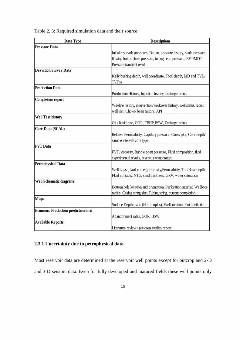
Table 2. 3: Required simulation data and their source
2.3.1 Uncertainty due to petrophysical data
Most reservoir data are determined at the reservoir well points except for outcrop and 2-D
and 3-D seismic data. Even for fully developed and matured fields these well points only
Data Type Descriptions
Pressure Data
Initial reservoir pressures, Datum, pressure history, static pressure
flowing bottom hole pressure, tubing head pressure, RFT/MDT
Pressure transient result
Deviation Survey Data
Kelly bushing depth, well coordinate, Total depth, MD and TVD/
TVDss
Production Data
Production History, Injection history, drainage points
Completion report
Wireline history, intervention/workover history, well status, latest
well test, Choke/ bean history, API
Well Test history
Oil / liquid rate, GOR, FBHP,BSW, Drainage points
Core Data (SCAL)
Relative Permeability, Capillary pressure, Cross plot, Core depth/
sample interval/ core type
PVT Data
FVF, viscosity, Bubble point pressure, Fluid composition, fluid
experimental results, reservoir temperature
Petrophysical Data
Well Logs ( hard copies), Porosity,Permeability, Top/Base depth
Fluid contacts, NTG, sand thickness, GRV, water saturation
Well Schematic diagrams
Bottom hole location and orientation, Perforation interval, Wellbore
radius, Casing string size, Tubing string, current completion
Maps
Surface Depth maps (Hard copies), Well location, Fluid definition
Economic Production prediction limit
Abandonment rates, GOR, BSW
Available Reports
Literature review / previous studies report

20
account for less than 1% of the reservoir volume. Because of this and the fact that most
reservoirs are highly heterogeneous, reservoir data are highly uncertain, especially at
reservoir locations between wells. The degree of uncertainty may vary from one variable to
another. The uncertainty of a parameter may result from difficulty in directly and
accurately measuring the quantity. This is particularly true of the physical reservoir
parameters which, at best, can only be sampled at various points, and are subject to errors
caused by presence of the borehole and borehole fluid or by changes that occur during the
transfer of rock and its fluids to laboratory temperature and pressure conditions (Walstrom,
1967).
2.3.2 Uncertainty in geophysical data
In the geophysical domain, uncertainties are linked to the acquisition, processing, and
interpretation of seismic data (Vincent, 1999 and Corre, 2000). Some of these
uncertainties, according to Sandsdalen et al., (1996) and Tyler, (1996), are:
i. Uncertainties and errors in picking horizons
ii. The difference between several interpretations
iii. Uncertainties and errors in depth conversion
iv. Uncertainties in seismic-to-well-tie
v. Uncertainties in pre-processing and migration
vi. Uncertainties in the amplitude map of the top reservoir

21
2.3.3 Uncertainty due to geological data
In the geological domain, the uncertainties are linked to the geological scheme, to the
sedimentary concept, to the nature of the reservoir rocks, their extent, and to their
properties (Corre, 2000). Uncertainty in any geological model is unavoidable given the
sparse well data and the difficulty in accurately relating geophysical measurements to
reservoir scale heterogeneities. Some of the known geological uncertainties are:
i. Uncertainties in gross rock volume
ii. Uncertainties in the extension and orientation of sedimentary bodies
iii. Uncertainties in the distribution, shape, and limits of reservoir rock types
iv. Uncertainties in the porosity values and their distribution
v. Uncertainties in the horizontal permeability values and their distribution
vi. Uncertainties in the layers Net-to-Gross Ratio
vii. Uncertainties in the reservoir fluids contacts
2.3.4 Uncertainty due to dynamic reservoir data
In the production area, there are uncertainties linked to any parameter that affects flow
within the reservoir, such as absolute and relative permeability, vertical to horizontal
permeability ratio (Verbruggen, 2002), fault transmissibilities, horizontal barriers,
thermodynamics, injectivity, and productivity index, well skin (Corre, 2000) and the
extension of horizontal and vertical barriers.

22
2.3.5 Uncertainty of reservoir fluids data
Uncertainties in the description of reservoir fluid composition and properties are of special
importance for the optimization of the processing capacities of oil and gas, as well as for
planning the transport and marketing of the products from the field (Azuka et al., 2009,
Meisingset, 1999). Some of the reservoir fluids uncertainties are:
i. Uncertainty in reservoir fluid samples which arises due to lack of representative
samples from the reservoir.
ii. Uncertainty in reservoir samples from different reservoir zones. Possible
variations in fluid properties in different parts of the field may introduce
uncertainty in the reservoir fluids description
iii. Uncertainty in the compositional analyses
iv. Uncertainty in volumetric measurements in the PVT laboratory. This is
considered to be of less importance compared with having representative fluid
samples
v. Uncertainties in the reservoir fluids’ interfacial tension. This may be of
importance due to its effect on the capillary pressure, and/or compositional
effects like re-vaporization of oil into injection gas (Meisingset, 1999).
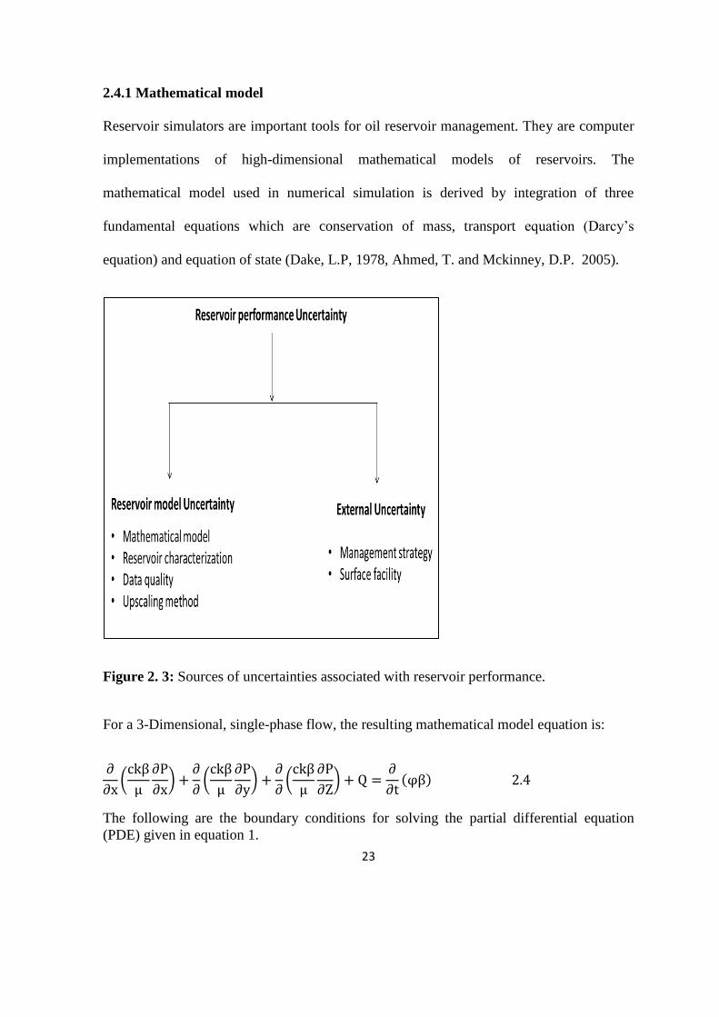
2.4 Reservoir Simulation Uncertainty
There is existence of varying degree of uncertainty associated with all data used in
reservoir modeling and simulation studies. Figure 2. 3 summarizes several uncertainty
sources associated with reservoir performance.
23
2.4.1 Mathematical model
Reservoir simulators are important tools for oil reservoir management. They are computer
implementations of high-dimensional mathematical models of reservoirs. The
mathematical model used in numerical simulation is derived by integration of three
fundamental equations which are conservation of mass, transport equation (Darcy’s
equation) and equation of state (Dake, L.P, 1978, Ahmed, T. and Mckinney, D.P. 2005).
Figure 2. 3: Sources of uncertainties associated with reservoir performance.
For a 3-Dimensional, single-phase flow, the resulting mathematical model equation is:
∂
∂x(ckβ
μ
∂P
∂x) +
∂
∂(ckβ
μ
∂P
∂y) +
∂
∂(ckβ
μ
∂P
∂Z) + Q =
∂
∂t(φβ) 2.4
The following are the boundary conditions for solving the partial differential equation
(PDE) given in equation 1.

24
P(x, y, z, 0) = Pi
∂P
∂x(0, y, z, t) = 0,
∂P
∂x(Lx, y, z, t) = 0
∂P
∂y(x, 0, z, t) = 0,
∂P
∂y(x, Ly, z, t) = 0
∂P
∂z(x, y, 0, t) = 0,
∂P
∂z (x, y, Lz,t) = 0
Equation 2.4 is a non-linear partial differential equation (PDE) which can not be easily
solved using analytical approach. Consequently, the PDE is converted to a numerical
model using Taylor series approximation briefly discussed below:
If we consider the function p(x) shown in Figure 2. 4, suppose we know the value of p(x)
at the point x and we know all the derivatives of p(x) at the point x. If we want to
approximate the value of p(x+∆x) at the point (x+∆x), we can do this with a Taylor series
as follows,
p(x+ x) = p(x)+ xp (x)+ x
2!p (x)+
x
3!p (x)+ +
x
n!p (x)+
2 3 nn
2.5
Where pn is the n
th derivative of p. This is an infinite series which is theoretically exact for
an infinite number of terms. However, if we truncate the series after n terms, then we
introduce a truncation error, et , (the remaining higher order terms which are not included).

25
Figure 2. 4: Illustration of Taylor series for pressure analysis
This truncation error is
t
n+1 n
e = p(x ) x
(n+1)!+
( )
1
2.6
and is equal to
t
n+1 n
e = p(x + ) x
(n+1)! (0 x)
( )
1
2.7
The function p(x) and all its derivatives must be continuous throughout the interval under
consideration. But, we often deal with discontinuities in both time and space. That limits
the Taylor series analysis.
If we take Pi as p(x), pi+1 as p(x+∆x), and pi-1 as p(x-∆x). We can expand Taylor series in
either direction as follows:
i+1 i
2 2
2
3
3
4
4p = p + x
p
x +
x
2!
p
x +
x
3!
p
x +
x
4!
p
x +
( ) ( ) ( )3 4
2.8
i-1 i
2
2
3
3
4
4p = p - x
p
x +
x
2!
p
x -
x
3!
p
x +
x
4!
p
x -
( ) ( ) ( )2 3 4
2.9
P(x+x)
x+xx
P(x)
x
P

26
The right-hand side now uses partial derivatives (evaluated at xi) since p is a function of
both x and t, p(x,t).
We have a couple of choices of approximations to ∆p/∆x:
Forward difference (from Eq. 2.8):
p
x
p - p
x
i+1 i
2.10
Backward difference (from Eq. 2.9):
)( xx
p -p
x
p 1-ii
2.11
Central difference (from Eqs. 2.8 and 2.9):
)( 2x)x(
p +p2 -p
x
p2
1+ii1-i
2
2
2.12
The derivation of the numerical model is done by replacing the partial derivatives in the
PDE with finite differences in equations 2.10 and 2.11 and evaluated at specific values of
x, y, z, and t. With this approximation the differential equation is transformed into an
algebraic equation that can be easily solved using matrix. The resulting finite difference
formulation is given in equation 2.13 and the numerical model can be represented in three
directions as shown in Figure 2. 5.
𝐴𝑃𝑖−1,𝑗,𝑘 + 𝐸𝑃𝑖,𝑗−1,𝑘 + 𝐺𝑃𝑖,𝑗,𝑘−1 + 𝐵𝑃𝑖,𝑗,𝑘 + 𝐶𝑃𝑖+1,𝑗,𝑘 + 𝐹𝑃𝑖,𝑗+1,𝑘 + 𝐻𝑃𝑖,𝑗,𝑘+1 = 𝐷 2.13
The resulting numerical equation includes pressure terms evaluated at two different points
in time. These times are the initial time, t = t0 and at a selected future time called time step,
t = t1. Knowing the pressure at the initial time, we have to solve the numerical equation for
pressure at the given time step. At subsequent time steps, pressure will be calculated at

27
multiple points in a three dimensional model. The resulting numerical equation coefficient
is solved using n x n matrix.
Figure 2. 5: 3-Dimensional Discretized Model
For one dimensional, single phase numerical model, a tri-diagonal matrix is formed. In a
four-cell system, the matrix is depicted as in equation 2.14:
b c
a b c
a b c
a b c
a b
p
p
p
p
p
d
d
d
d
d
1 1
2 2 2
3 3 3
4 4 4
5 5
1
2
3
4
5
1
2
3
4
5
2.14
This matrix representation consists of three non-zero diagonals and is easily solved.
General Implicit Methods: This is also a mixed explicit/implicit method, but is more
flexible than the Crank-Nicolson (C-N) method.
(1- )1
( x )( p -2 p + p ) +
1
( x )( p -2 p + p ) =
1
t( p - p )
2 i-1
n
i
n
i+1
n
2 i-1
n+1
i
n+1
i+1
n+1
i
n+1
i
n
2.15
Weighting factor: (0 1)

28
For:
= 1 (Implicit)
= 0 (Explicit)
= 1/2 (C-N)
Truncation Error: ((x) 2
, (t)) (generally)
Only the implicit method is unconditionally stable (for any time step size). The explicit
method is stable only for sufficiently small time steps, which are generally impractical.
Although the Crank-Nicholson method has higher order accuracy, it is on the borderline of
instability and is conditionally stable for practical purposes. Therefore, the implicit
method is the standard in reservoir simulation. If more accuracy is required, smaller time
steps are used.
The computation time needed to obtain pressure solution (Pn+1) for the implicit
approximation is more than that for the explicit method. The problem complexity increases
with increased number of dimensions and for multiple phases present. For two phases, the
fluid flow equation applies to each flowing phase individually such that at each time step
there are two unknowns to be solved, Po, and Sw in each grid block.
Three errors that are inherent in numerical model as a result of PDE discretization include:
i. Truncation errors
ii. Round-off errors
iii. Stability errors
The truncation error results from the substitution of the partial derivatives in the
differential equation with approximate finite differences (Peaceman, D.W, 2003). As a

29
result, it is an approximate solution which does not mimic the actual reservoir exactly.
Round-off error, on the other hand, is a result of using a computer to solve the numerical
model because the computer cannot represent real numbers accurately. Stability error
consists of the approximation method used in transforming the PDE into a numerical
model and the PDE itself. Instability in numerical solution leads to one error translating to
another error (truncation or round-off errors, respectively). As the error increases, the rate
of error growth increases so that the error growth gets so large that the solution is lost.
Apart from the algorithms used to generate the numerical model, model uncertainties can
also arise from the type of reservoir simulator used. The simulator used can either be mass
balance or streamline, finite difference or finite element. The inherent uncertainty results
from the inadequacy to completely translate the continuous mass balance and flow
equations into discrete approximates and the use of a computer to solve the equation. Due
to all these, the numerical model that is used in reservoir simulation contains uncertainty
which need to be quantified.
2.4.2 Up-scaling Uncertainty
A variety of papers was published that address specific aspect of how best to capture
critical geological heterogeneities in earth models prior to and during upscaling for
dynamic simulation (Castellini et al., 2003, Apaydin et al., 2005, Stern, 2005). After
acquisition and interpretation of the seismic volume, the geologist builds the static model.
Because the model built is usually a fine scale level it is computationally expensive to
investigate reservoir flow behavior using such model. Consequently, the geological model

30
is upscaled into a coarse scale model generally called a reservoir simulation model in order
to evaluate the reservoir flow behavior.
Upscaling technique is needed to transform the fine grid into coarse grid model (see Figure
2. 6). During Upscaling, reservoir properties are upscaled so as to reduce the number of
grid blocks and facilitating simulation runs (Durlofsky, L.J, 2003, Hui, M., 2004, Ates, H
et al., 2005, Lambers, J. and Gerritsen, M, 2005, Sablok, R. and Aziz, K, 2005). The fine
grid model is employed to characterize a reservoir although in most modeling the model
areal resolution is still coarse due to computational costs for the finer grids. On the other
hand, the coarse grid model is used to evaluate reservoir performance prediction because of
time constraints and available resources. To evaluate reservoir performance using fine grid
model can also be limited by available computer capability and costs. As a result,
upscaled/coarse grid model of the fine-scale model is required. A number of upscaling
techniques are available in the literature. The different approaches can be classified
according to two broad methods (Durlofsky, 2003).
i. the type of parameter to be upscaled, and
ii. the method of computing the parameter

31
Figure 2. 6: Process in upscaling
These methods have various degrees of limitations in the ability to translate a fine-scale
model into a coarse-scale model. Irrespective of the particular upscaling technique
employed to generate the coarse model, utmost care should be taken to ensure that the
upscaled model input parameter(s) is equivalent to the fine scale model parameter. For
example, accurate upscaling of residual oil saturation and initial water saturation are vital
because these two parameters determine the amount of oil that can be recovered from the
reservoir. Some parameters such as porosity and saturation are accurately upscaled using
simple volume averaging techniques. While absolute and relative permeability have varied
upscaling algorithms. As a result, significant amount of uncertainties exist when
permeabilities are upscaled from fine scale into coarse grid. Recognizing the fact that
upscaling uncertainty exists, there is a need for proper quantification of upscaling
uncertainty, which is important for better reservoir performance prediction.

32
Upscaling of fine scale model into a coarse scale model is conducted in both black oil and
compositional simulation. See the work by Durlofsky, (2003) for detailed literature on
upscaling of black oil model. Less work has been done on upscaling of compositional
simulation; most of the work done so far on compositional upscaling (Ballin et al., 2001
and Hui et al., 2004) has been the adjustment of K-value flash calculation in order to
account for using coarse grid to represent fine scale. This K-value adjustment resulted in
Alpha factor method which serves as modifiers (Li and Johns, 2005). The modifiers are
introduced into numerical simulation flow equation to relate fluid composition flowing out
of the grid to the fluid composition within the grid.
2.4.3 Uncertainty due to Geostatistics
Estimation is one of the major applications of geostatistics, the other being conditional
simulation. The objective is to estimate the variable of interest at a location Xo for which
no datum has been measured, using the data measured at other locations Xi distributed in
space. The major limitation of linear estimation methods stems from the fact that the
structure of the heterogeneity as represented by the Variogram, the covariance function or
the correlation coefficient function has not been taken into account and uncertainty is
introduced to the estimation. Geostatistics uses a probabilistic framework to make
estimations and in so doing provides estimates that honor the correlation structure of the
heterogeneity (Ratchkoviski et al., 1999). It also provides quantitative assessment of the
reliability of the estimates by providing both the estimate and its confidence limits. The
common methods include the Variogram and Kriging.

33
2.4.3.1 Kriging
Kriging is a 3-D estimation program for variables defined on a constant volume support.
Estimation can either be performed by simple Kriging (SK), ordinary Kriging (OK),
Kriging with a polynomial trend (KT) or simple Kriging with a locally varying mean
(LVM). LVM is a variant of Kriging, in which it is assumed that the mean m (U) is not
constant but is known for every U. In all geostatistical estimation, the variable of interest is
treated as a stationary random function with a normal probability distribution. If the
measured data do not exhibit a normal distribution, they must first be transformed into a
normal distribution before proceeding further. Such a transformation can always be done
by using the cumulative distribution function of the data and the cumulative distribution
function of a standard normal distribution with a mean of zero and a standard deviation of
1. The criteria used in ordinary Kriging to obtain the best estimate are (1) the estimate
should be unbiased and (2) the estimation error should have minimum variance.
Ordinary Kriging is a Best Linear Unbiased Estimator (BLUE) which can be derivation in
terms of the covariance function or Variogram function. The estimation is a classical
problem of optimization, which can be solved by the method of Lagrange multipliers.
The objective function is to minimize
𝜎𝑒2 = 𝜎2 + ∑ ∑𝜆𝑖𝜆𝑗𝐶(ℎ𝑖𝑗) − 2∑𝜆𝑖𝐶(ℎ𝑖𝑜)
𝑁
𝑖=1
𝑁
𝑖=1
𝑁
𝑖=1
2.16
or

34
𝜎𝑒2 = ∑∑𝜆𝑖𝜆𝑗𝛾(ℎ𝑖𝑗) + 2∑𝜆𝑖𝛾(ℎ𝑖𝑜)
𝑁
𝑖=1
𝑁
𝑗=1
𝑁
𝑖=1
2.17
Subject to
∑𝜆𝑖 = 1 2.18
𝑁
𝑖=1
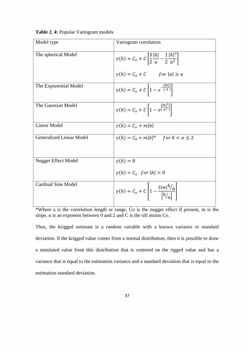
2.4.3.2 Variogram
The Variogram is used to quantify the correlation structure of the variable of interest for
the purpose of estimation and conditional simulation. The Variogram of the sample data is
known as the experimental Variogram. After computing the experimental Variogram, a
smooth theoretical Variogram model is usually fitted to the experimental Variogram and
the model is then used for estimation. The estimation process involves the solution of a set
of linear simultaneous algebraic equations, whose coefficients are derived from the
Variogram. Unless the Variogram is well behaved, the simultaneous equations may not
have a solution. Hence, the need to fit a smooth and well behaved theoretical model to the
rough experimental Variogram for the purpose of estimation.
The Variogram increases as the values of properties measured on a set of samples become
more dissimilar. The formula for the "semivariogram" is written conventionally in terms of
a "lag" h, and a set of observations z, known as attributes, made at a number of locations, s.
The difference in attributes for pairs of spatially separated samples is compared for
increasing values of the lag using;

35
𝛾(ℎ) =1
2𝑁(ℎ)∑(𝑧(𝑥𝑖 + ℎ) − 𝑧(𝑥𝑖))
2 2.19
𝑁(ℎ)
𝑖=1
Where the N(h) is a count of the possible pairing at each lag used to compute the function.
The Variogram is truncated at the value of lag where the diminishing number of possible
pairings loses statistical significance.
Figure 2.7 shows an ideal Variogram. It starts at zero and increases with increasing lag
distance until a certain distance is reached at which it levels off and becomes constant. The
lag distance at which the Variogram levels off (a in the figure) is defined as the correlation
length, or the range of influence, and the value of the Variogram at this point is called the
sill. The sill is the semivariance of the entire data set. Thus, hidden in the Variogram are
the variance and standard deviation of the data set, the usual measures of heterogeneity of
ordinary statistics. If the correlation length is zero, the spatial distribution of the property is
fully random. With increasing correlation length, the range of influence of one value on its
neighbors increases up to the correlation length. At lag distances beyond the correlation
length, the data are no longer correlated. Table 2.4 summarizes the popular Variogram
models.
2.4.3.3 Conditional simulation
Kriging gives a smooth estimate because the estimate is a weighted average of the sample
data. Such average can never be larger than the largest sample value nor can it be smaller
than the smallest sample value. Thus, Kriging eliminates local variability. If such local
variability is important, then it can be incorporated into the estimated values using
conditional simulation. The idea behind conditional simulation is that each of the estimates

36
obtained from Kriging was associated with an uncertainty in the estimated value measured
by the estimation variance or the estimation standard deviation.
Figure 2. 7: Typical Variogram showing Variogram characteristics
0.00
0.50
1.00
1.50
2.00
2.50
3.00
0 1 2 3 4 5 6 7
Sem
ivari
ogra
m
Lag, h (ft)
γ(h)
SPH(2.7,5)
Nugget = 0.05
Series4
Range = 5
37
Table 2. 4: Popular Variogram models
Model type Variogram correlation
The spherical Model 𝛾(ℎ) = 𝐶𝑜 + 𝐶 [
3
2
|ℎ|
𝑎−
1
2
|ℎ|3
𝑎3]
𝛾(ℎ) = 𝐶𝑜 + 𝐶 𝑓𝑜𝑟 |𝑎| ≥ 𝑎
The Exponential Model 𝛾(ℎ) = 𝐶𝑜 + 𝐶 [1 − 𝑒
−[|ℎ|𝑎
]]
The Gaussian Model 𝛾(ℎ) = 𝐶𝑜 + 𝐶 [1 − 𝑒
[|ℎ|2
𝑎2 ]]
Linear Model 𝛾(ℎ) = 𝐶𝑜 + 𝑚|ℎ|
Generalized Linear Model
𝛾(ℎ) = 𝐶0 + 𝑚|ℎ|𝛼 𝑓𝑜𝑟 0 < 𝛼 ≤ 2
Nugget Effect Model 𝛾(ℎ) = 0
𝛾(ℎ) = 𝐶𝑜 𝑓𝑜𝑟 |ℎ| > 0
Cardinal Sine Model
𝛾(ℎ) = 𝐶𝑜 + 𝐶 [1 −
𝑆𝑖𝑛(ℎ 𝑎⁄
|ℎ 𝑎⁄ |]
*Where a is the correlation length or range, Co is the nugget effect if present, m is the
slope, α is an exponent between 0 and 2 and C is the sill minus Co.
Thus, the krigged estimate is a random variable with a known variance or standard
deviation. If the krigged value comes from a normal distribution, then it is possible to draw
a simulated value from this distribution that is centered on the rigged value and has a
variance that is equal to the estimation variance and a standard deviation that is equal to the
estimation standard deviation.
38
In other words, conventional geostatistical estimation procedures are filtering techniques.
They filter out high frequency information and capture only low frequency data. Many of
the reservoir properties exhibit short scale variability (e.g., permeability), which may not
be captured by conventional geostatistical techniques. Sequential simulation procedures, in
contrast, capture this small scale variability (Journel and Albert, 1990). The two principal
sequential simulation techniques are Sequential Indicator Simulation (SIS) (Journel and
Alabert, 1990), and Sequential Gaussian Simulation (SGS) (Alabert, 1987). SIS transforms
the data into discrete indicator variable before simulation, whereas, SGS transforms the
data into continuous Gaussian domain before simulation. Although difficult to generalize,
SIS has been found to be most useful in simulating geological facies or rock types,
whereas, SGS has been found to be most useful in simulating continuous variables such as
porosity, permeability, saturation, etc.
The algorithm for performing such a stochastic simulation known as Sequential Gaussian
Simulation (SGS) uses estimation equation given in equation 2.20.
𝜃𝑠𝑖 = 𝜃𝑖∗ + 𝜃𝑒𝑖𝑍𝑖 2.20
Where 𝜃𝑠𝑖 is the simulated value at location i, 𝜃𝑖∗ is the kriged value at location i, 𝜃𝑒𝑖 is
the standard deviation or the square root of the estimation variance at location i and Zi is a
standard normal variate with μ = 0 and σ = 1 drawn for location i.
The problem with geostatical modeling is that it is computationally difficult to condition
the entire model with dynamic data. Also, it is difficult to utilize traditional history match
process to condition all the geostatistical models (Alhuthali et al., 2006). Gaussian
simulation, Kriging, Kriging with external 3D drift and Collocated cokriging are some of

39
the techniques that have been found useful for generating multiple descriptions of the
reservoir.
2.5 Management of Reservoir Uncertainties
Managing reservoir uncertainties implies reduction of uncertainties or assessment of
reservoir uncertainty. Uncertainty reduction could be achieved by carefully planning a
timely data acquisition campaign. Efforts should be made to guarantee that the data are
acquired following best practice procedures. Assessment of reservoir uncertainties would
allow asset teams to analyse the risk associated with development projects.
2.5.1 Uncertainty assessment of static reservoir parameters
Static geological modelling is associated with uncertainties in reservoir geometry and
heterogeneities that have a major impact on reservoir bulk and pore volume as wells, as
fluids flow in these reservoirs. The two largest static uncertainties – the reservoir geometry
as defined by reservoir faults and horizons and the petrophysical property distributions –
may be assessed and quantified by geostatistical methods (da Cruz, 2004). Modelling the
connectivity of permeable and impermeable zones can be highly uncertain. Geostatistical
methods provide means for incorporating connectivity through the indicator variograms,
and help in describing the probability of lithologies at different locations resulting in
different connectivity (Srivastave, 1990).

40
2.5.2 Uncertainty assessment of dynamic reservoir parameters
After building the most representative model, a few realizations are generated using
geostatistics. These multiple realizations can be ranked to reduce the number of models for
further processing with numerical simulator (Friedmann, 2003). Traditionally, the variation
of one-parameter-at-a-time approach is used as a sensitivity analysis to assess effects of
uncertainties in various dynamic parameters on chosen responses. The dynamic simulation
model is validated by matching production history data of existing wells to simulation data
by varying selected dynamic parameters such as aquifer pore volume and connectivity,
relative permeability data, faults connectivity, or Kv/Kh data. Typically, one or two
parameters are varied at a time (Vincent, 1999). This process is tedious and for large fields
it becomes close to impossible to investigate relationships between the model responses
and variations of different reservoir input parameters. A procedure that combines all
uncertainty and allows transferring uncertainties through the numerical flow model up to
the production forecasts is highly desired (Ballin, 1993).
2.6 Overview of History Matching
History matching is defined as an act of adjusting a model of a reservoir until it closely
reproduces the past behavior of a reservoir. This is a common practice in oil and gas
industry in order to have reasonable future predictions. Computation time (and cost)
becomes important when we encounter problems with a large number of unknown
parameters and will be even more critical when an estimation of gradients is needed.
Several methods have been introduced for speeding-up optimization. One efficient way to
accomplish this is to introduce a parallel or distributed computing framework (Schiozer

41
and Sousa 1997, Schulze-Riegert et al., 2003). Parallelization is common in global
optimization algorithms but can be also effective for computing gradients. The gradient of
the data mismatch can also be calculated by the means of using adjoints (Ruijian et al.,
2003, Dong and Oliver 2005 and 2008).
2.6.1 Traditional history matching
Traditional history matching is performed by trial and error. Reservoir engineers analyze
the difference between simulated and observed value and manually change one or a few
parameters at a time in the hope of improving the match. In such an approach, reservoir
parameters are updated manually and often in two steps: the pressure match and the
saturation match (Mattax and Dalton 1991). The quality of this type of history matching
largely depends on experience and the amount of the budget. It is important to emphasize
that the key elements of traditional History Matching are viable, i.e., integration of domain
knowledge and heuristics. Best practices (Selberg, 2007) are integrated into modern
workflows. But the tools cannot do without them. The use of modern tools allows
structuring of the History Matching workflow, and methods are adopted to interpret the
reservoir simulation response and help to guide the decision process.
Since reservoirs are usually very heterogeneous, there are hundreds of thousands of grid
blocks in a typical reservoir simulation model to estimate reservoir parameters in high
resolution. Therefore, manual history matching is often not reliable for long periods and is
always associated with many uncertainties, so computers are employed to automatically
vary the parameters. This procedure is called computer aided (semi-automatic) history
matching and resulted to multiple solutions. Semi-automatic history matching is defined as

42
construction of an initial model with an initial approximation of the reservoir parameters
which then goes through a systematic process reduction of an objective function that
represents the mismatch between observation and calculated response by perturbing the
relevant parameters (Guohua et al., 2004).
One of the first studies on history matching was done by Kruger, (1961). He calculated the
areal permeability distribution of the reservoir. Jacquard and Jain, (1965) developed a
method to automate the history matching. Chavent et al., (1973) studied history matching
in single phase oil reservoirs. The objective was to minimize the difference between
observed and actual pressures at the wells with the permeability-thickness product and
porosity-thickness product as adjustable parameters. Fasanino et al., (1986) studied single-
phase history matching of 2D gas reservoirs using the adjoint method in combination with
geostatistical information and the pilot point technique. Bi et al., (2000) studied the
conditioning of three-dimensional stochastic channels to pressure data in single-phase
reservoirs. Li et al., (2003) studied history matching of three-dimensional, three-phase
flow production data. The objective was to minimize the mismatch in flowing wellbore
pressure, producing gas oil ratio (GOR) and water oil ratio (WOR).
2.6.2 Optimization Techniques
There are several optimization methods applied in reservoir model simulation and History
Matching projects. Commercial and proprietary optimization frameworks and techniques
used for real full-field reservoir simulation studies include the following: evolutionary
Algorithms (Williams, 2004, Schulze-Riegert, 2007), gradient techniques (Roggero, 1998),
response surface modeling and optimization on the response surface (Little 2006), hybrid

43
schemes which couple different optimization techniques (Castellini, 2006). The most
prominent techniques that are receiving a high level of attention in the research community
presently are Ensemble Kalman Filter Techniques (Evensen, 2007, Evensen et al., 2007).
Either method has advantages and limitations. An extensive review first presented in the
mid 90’s is given by Wen et al., (2005).
From various review studies, any optimization method must be transparent, and results
must directly relate to verifiable workflows, in order to establish trust and confidence. For
instance, the evolutionary algorithms that satisfied these requirements (Wen et al., (2005),
can provide a methodology for challenging deployment of algorithms for an increasing
number of problems which become more and more complex and require solutions in no
time. The literature reports multiple implementations of Evolutionary Algorithms (Eiben,
2003). The underlying principle is derived from a population of individuals, the
environmental pressure that induced natural selection (survival of the fittest), which leads
to an increase in the fitness of the population. Genetic Algorithms are the most widely
known type of Evolutionary Algorithm (Gen, 2000, Eiben, 2003).
2.6.3 History matching using response surface methodology
The goal is finding input variable value of the flow simulation that result in a value as near
as possible of the observed data. If many observed are available, it is possible to aggregate
them into an objective function:
OF =1
2∑Wi(di
obs − disim)2
n
i=1
2.21

44
In which di are the observed and simulated data and Wi are the weight assigned to the data.
Minimization of the OF means that to match the reservoir production history. Here, history
matching process uses the following polynomial;
OF = β0 + β1X1 + β2X2 + β3X1X2 + β4X12 + β5X2
2 2.22
Accordingly, history matching may be done by finding the minimum value for the function
equation 2.22. Experimental Designs and Response Surface Modeling (RSM) are often
used in diverse workflows to quantify uncertainties and to investigate the propagation of
parameter uncertainties by using Monte Carlo sampling techniques. At the same time, the
technique are been used to approximate complex simulation models for a number of
simulated responses. The whole suite of available optimization methods can then be used
to optimize responses based on surrogate models. Full field reservoir simulation results are
then captured in a proxy model with a number of chosen design (uncertainty) parameters.
There is numerous response modeling techniques described in the literature (Manceau et
al., 2001, Montgomery, 2005). Most of the available tools for response modeling generate
second order polynomials that are usually, highly dimensional and may not represent a
non-linear system well. In order to handle a large number of uncertainty parameters, the
polynomial is typically reduced by identifying less sensitive terms, which are excluded
from the calculation. Thus, for any history matching (HM) workflow, key parameters are
identified based on their contributions to the objective function definition. Depending on
the number of parameters, the number of terms increases rapidly. For 20 uncertainty
parameters a second order polynomial will consist of 20 linear, 20 quadratic and 190 cross

45
terms (230 contributions). Once a response surface of acceptable quality is obtained, any
optimization technique can be used to identify optimal solutions on the response surface.
Identified solutions are verified through full field simulations, and update the database for
recalculating an improved proxy model. In all practical application workflows this is an
iterative procedure and prior information may be included in a Bayesian formulation which
is used in the updating process.
2.7 Proxy Modeling
2.7.1 Experimental design
The increasing demand for systematic and consistent methodologies for analyzing
uncertainty and associated effects on investment decisions is responsible for increasing
usage of DoE in reservoir management (Vanegas et al., 2006). To be able to harness the
benefits associated with Design of Experiment (DoE), users must apply it wisely failure of
which causes delay in decision making process. Important areas of application of DoE in
petroleum engineering include uncertainty screening and uncertainty quantification
(Cotento et al., 2005, Peak et al., 2005). With DoE one can significantly reduce the
number of simulations. Previous screening methodologies (Steagall and Schiozer, 2001)
consider static sensitivity analysis. Though still applicable for some studies, the dynamic
behavior of the sensitivity is important to observe because different uncertainty attributes
may have different time of influence on reservoir performance.
Recent research and applied reservoir characterization and modeling projects have focused
on the application of DoEs and Response Surface techniques (Almeida et al., 2003, Peng

46
& Gupta, 2003, Amudo et al., 2008). Successes recorded from their usage have been found
to depend on a number of factors. These include, available time, number of uncertainty
factors, the study objectives and amount of details required from integrated reservoir
simulation studies. There are several types of experimental designs. Morris, (2000)
classified them into fractional factorial design (FRFD), optimal design and Latin
Hypercube Design (LHD). The first two classes according to Box et al., (2005) and
Montgomery et al., (2005) are extensively used in the area of physical experiments for
model development. LHD is efficient design that allows representation of entire parameter
range in the design matrix. Its construction is based on the idea of stratified sampling
which requires search algorithms and pre-specified optimality criteria (Box et al., (2005).
The underlying assumptions to use 2-level factorial designs are that the 3-factor
interactions and higher are negligible. Consequently, most of the experiments are omitted
from the analysis and therefore seldom used for construction of response surfaces
especially when factors are many and interactions are envisaged. To illustrate this, if we
consider 7 parameters system of 27=128-runs for typical full design. Among the 127
degrees of freedom in the design, only 7 are used to estimate the linear terms and 21 to
estimate the 2-factors interactions. The remaining 119 degrees of freedom are associated
with three-factor interactions and higher that are supposed to be negligible. In practice, if
the number of factors ranges between 2 to 15, fractional factorial can be used to screen the
significant few by estimating the main effects and interactions. There are various possible
fraction designs: 64-, 32- or 16-run design. The 16-run design usually is preferred since
this is the cheapest design with resolution IV that is available for uncertainties higher than

47
eight. Two level Plackett-Burman (PB) designs have been used in the context of classical
statistical experiments for screening purposes.
PB designs cannot be used when higher number of levels is required or where simulator
proxies development remains the focus of the study. One variable at a time is a screening
method involving varying a parameter values between its minimum (-1) and maximum
(+1) range within the parameter space. The degree of the displacement from the base case
of resultant response indicates the extent of influence the parameter has on the measured
response. One variable at a time method is a static sensitivity common in classical
laboratory experiments. However, its application for screening large number of
uncertainties has been reported (Fatemeh and Nassar, (2012).
The 3-level DoE methods are high resolution algorithms for response surface construction.
Central Composite Design (CCD) consists of a factorial design with the corners at +1 of
the cube, augmented by additional “star” and “center” points, which allow the estimation
of the second order polynomial equation (Allen et al., 2003). Like CCDs, Box-Behnken
designs are a family of 3- level designs and can be constructed by the combination of
factorial and incomplete block designs (Montgomery et al., 2005). The application of 3-
level full factorial is limited only to four factors or lower due to the associated large
number of runs for large number of uncertainty. However, 2-level factorial designs
(fractional designs) have also been used where 3-level full factorial is infeasible for
response surface construction (Aigbodion, et al., 2010 and Mu’azu et al., 2012).
Despite its wide applications in the petroleum industry, the DoE method has seldom been
compared with MC simulations for uncertainty quantification. DoE provides a proxy of
48
reservoir models, and it has been used to speed up the history-matching process (Amudo et
al., 2008; Schaaf et al., 2008). The DoE method is more efficient than the direct MC
method. Multilevel designs increase the number of simulations significantly, and some
mixed designs are more efficient (Kalla and White, 2007). However, a key disadvantage of
the DoE approach is that it does not take into account the full probability distributions of
the parameters consistently while creating the response surface. Further, because all
samples are equally weighted for response-surface generation, there is an inherent
assumption that the distributions of these parameters are uniform. As a result, the DoE
method may not be appropriate when parameter distributions are arbitrary, which is
common in real-world applications.
2.7.2 Analysis of variance
The analysis of variance (ANOVA) is a hypothesis test with the null hypothesis (Ho) that
the factor has no effect on the simulator output. The test statistic (F) in an ANOVA is a
Fisher distributed random variable with a certain number of degrees of freedom. A large
value on the observed test statistic (Fobs) indicates that the factor has no effect. The Pr-
significance value is defined as the probability of having a test statistic that is at least large
as the observed test statistic:
𝑃 = 𝑃(𝐹 ≥ 𝐹𝑂𝐵𝑆) 𝑜𝑡ℎ𝑒𝑟𝑤𝑖𝑠𝑒 𝑡ℎ𝑒 𝑛𝑢𝑙𝑙 ℎ𝑦𝑝𝑜𝑡ℎ𝑒𝑠𝑖𝑠 𝑖𝑠 𝑡𝑟𝑢𝑒) 2.23
A small Pr-value means that the probability of getting the observed test statistic, given that
the null hypothesis is true, is very unlikely. The null hypothesis is then rejected, and we
assume that the factor has an effect.

49
The following equations are computed. ANOVA partitions total Sum of Squares SST into
3: SSM, SSE and SSR
𝑆𝑆𝑇 = 𝑆𝑆𝐸 + 𝑆𝑆𝑀 + 𝑆𝑆𝑅 2.24
Where,
𝑆𝑆𝑇 = ∑[𝑌𝐼 − 𝑌𝑃𝑅𝐸𝐷]2𝑁
𝐼=1
2.25
𝑆𝑆𝑅 = ∑[𝑋𝑖 − ]2𝑛
𝑖=1
2.26
𝑆𝑆𝐸 = ∑(𝑌𝑖 − )2 − 𝑏𝑖2 ∑(𝑋𝑖 − )2 2.27
𝐹𝑜 =
𝑆𝑆𝑅(𝑝 − 1)⁄
𝑆𝑆𝐸(𝑛 − 𝑝)⁄
2.28
𝑅2 = 1 −𝑆𝑆𝐸
𝑆𝑌𝑌 2.29
𝑆𝑌𝑌 = 𝑆𝑆𝑅 + 𝑆𝑆𝐸 2.30
𝑅𝑎𝑑𝑗2 = 1 −
𝑆𝑆𝐸(1 − 𝑝)⁄
𝑆𝑌𝑌(𝑛 − 1)⁄
2.31
2.7.3 Response surface methodology
RSM is one of the simplest techniques for building proxy models. It relates output
variables to input parameters over the entire parameter space. They are usually constructed

50
with regression method (Friedmann et al., 2003, Allen et al., 2003). The use of response
surface models is detailed by Dejean and Blanc, (1999). When calibrated, the Response
Surface Model is used to determine a set of design variables that optimize a response
(Risso et al., 2007, Ogbalor and Peacock, 2010). A multi-parameter regression method is
used to build regression models that link the parameters and the responses. The main
interest is to save cost by using the obtained equations for response prediction in place of
time costly simulation. The design selected however must have enough coverage so that all
the coefficients of the model are estimated accurately and are of predictive capability. An
example of the interactive model is:
Response = a0 + a1X1 + a2X2 + a3X3 + a12X1X2 + a13X1X3 + a23X2X3 2.32
where X1, X2, and X3 represent the main effects and X1X2, X2X3, and X1X3 account for
interaction between the parameters. For modeling studies, where a non-linear relationship
exists between the response and factors, the quadratic equation is constructed (equation
2.33).
Response = a0 + a1X1 + a2X2 + a12X1X2 + a11X12 + a22X2
2 2.33
Where a0, a1… a22 are constant coefficients obtained by fitting a set of numerical
simulations. This equation is second order. In matrix notation, the x equations obtained
using the models are grouped together and expressed as:
y = Xβ + ε 2.34
X is a (n*p) matrix called the model matrix, y is the n*1 vector of observations of the
response, n denotes the number of experiments, p is the number of terms in the model and

51
ε is any source of variability not accounted for in y. The term, β, is a vector whose
elements are the unknown regression coefficients. It is estimated using the ordinary least
squares method. This method estimates a vector b by minimizing the sum of the squared
residuals. The errors or residual vector is defined as the difference between the observed
and the fitted values,
e = y − y 2.35
where the fitted model is written as
y = Xb 2.36
and is obtained by minimizing L where L is given as
L = ∑εi2 = εtε = (y − Xβ)t(y − Xβ)
n
i=1
2.37
b is an unbiased estimate of β. The expression for b is given by
b = (XtX)−1Xty 2.38
The covariance of b is very important because it is directly related to the quality of the
model. It is a function of the model matrix X and the standard error deviation such that
Cov(b) = σ2(XtX)−1 2.39
Where
σ = √∑ (yi − yi)2n
i=1
n − p 2.40

52
The use of Artificial Neural Network (ANN) and Krigging has been reported for resolving
nonlinearity issues (Peng and Gupta, 2004). However, appropriate selection of
experimental design and sampling techniques can significantly improve model reliability
(Yeten et al., 2005). Yeten, (2005) studied different experimental designs and proxy-
models and their capability to predict uncertainties in selected field performance. A good
result was reported in application of Kriging and splines proxy-models with Latin
hypercube design. But the same types of proxy-models gave worse results for traditional
designs (e.g. Placket- Burman, Central Composite and D-optimal designs). Yet, traditional
designs are still popular for proxy modeling in petroleum engineering. The reason is
largely due to the ease of obtaining response surfaces whenever experimental design is
used. The creation of proxy-models of a high quality is therefore related to the selection of
appropriate experimental design algorithms, the quality of the input dataset as well as the
degree of non-linearity of input-output relationship.
2.7.3 ANN and Fuzzy Inference system
Artificial Neural Network (ANN) according to Mohagheh, (2000) addresses the problem of
non-linearity in the input-output relationship. ANN has been presented as an important tool
that can be applied to map the response surface in the multidimensional spaces of a
reservoir model (Cullick et al., 2006). The mapped response is then used as a substitute of
reservoir simulation runs during history matching and production forecast. Some of the
limitations of ANN are highlighted by Mohaghegh, (2000), and Olatunji et al., (2011).
Recent studies have shown that these limitations can be overcome through the application
of another Sensitivity Based Linear Learning Methods (SBLLM) in the conventional Feed

53
Forward Neural Network (FFNN) and the use of Fuzzy logic (Sampaio et al., 2009).
According to Olatunji et al., (2011), SBLLM is an improvement that was able to resolve
the instability problem. Fuzzy logic as pointed out by Salam et al., (2011), has ability to
capture knowledge from data that is inherently imprecise and maintaining a high level of
performance in the presence of uncertainty. The original Back-propagation method used in
Nets was found to exhibit slow convergence due to large search space dimensions for
learning. Fuzzy Inference System (FIS) employs hybrid-learning rules for training process.
Adaptive Neuro-Fuzzy Inference System (ANFIS) employs hybrid-learning algorithm.
Hybrid algorithm is a combination of gradient descent and the least-squares method. In the
forward pass of the hybrid learning algorithm, node outputs would go forward until last
layer and the consequent parameters would be identified by the least-squares method
(Roger, 1993). In the backward pass, the error signals propagate backwards and the
premise parameters would be updated by gradient descent. The consequent parameters are
optimized under the condition that the premise parameters are fixed. Thus, hybrid approach
converges much faster than conventional backward propagation as applied to ANN.
2.8 Uncertainty Quantification
With the emergence of new methods for comprehensive evaluation and comparison of risk
and uncertainty associated with investment choice, decision-makers are faced with
challenges of making choice of methods so that they can be properly guided on the
potential profitability and likelihood of achieving various levels of Return on Investment
(ROI). In this section we will briefly explain different uncertainty quantification techniques
and their characteristics.

54
2.8.1 Monte Carlo Method
Monte Carlo (MC) simulation is a powerful statistical method that has been used for more
than half a century. It has been applied extensively in the petroleum industry for decades. It
is employed as an alternative to numerous full-scale reservoir simulations in petroleum
industry (Amudo et al., 2008). Other areas of its successful applications include reserves
estimation, material balance analysis, work-over risk assessment and producing property
estimation. MC simulation is extensively used for uncertainty quantification (Zhang,
2002). In the MC method, a large number of realizations of the random inputs are
generated and solved to obtain a set of model outputs, which can be further analyzed
statistically. The direct-sampling MC method is conceptually straightforward and easy to
implement. However, its main disadvantage is the requirement of large computational
effort because of the large number of model simulations needed to obtain statistically
accurate results. It makes MC simulations prohibitive in most real applications of reservoir
simulation, especially for large-scale problems.
One of the critical stages in Monte Carlo is the assignment of distribution functions to
different independent parameters. There are several possibilities, different input variables
might have different statistical distributions (normal, lognormal, triangular, uniform), or all
input variables having the same statistical distribution but with different properties (mean
and standard deviation). Those probability density functions have to be determined by
trial-and-error while performing Monte Carlo simulation. This is another limitation of
using this technique. There are several probability distributions in statistics, but only the

55
normal and log normal distributions are most commonly observed in petrophysical
properties.
Normal (Gaussian) distribution function
The probability density function for a normal distribution is given by:
P(x) =1
σ√2πexp [−
(x − μ)2
2σ2] for − ∞ ≤ x ≤ ∞ 2.41
Where x is a random variable and μ is the mean, σ2 is the variance and σ is the standard
deviation of the distribution. The distribution is characterized by two parameters, the mean
(μ) and the standard deviation (σ). The cumulative distribution function for a normal
distribution is defined as
F(x) =1
σ√2π∫ exp [−
(x − μ)2
2σ2] dx
x
−∞
2.42
Log normal distribution function
The probability density function for a log normal distribution is given by
P(x) =1
σ√2π
1
xexp [−
(lnx − μ)2
2σ2] 2.43
where x is a random variable and μ is the mean, σ2 is the variance and σ is the standard
deviation of lnx. The mean, τ, and the variance, ω2, of the log normal distribution are
related to the parameters of lnx as
τ = exp(μ +σ2
2) 2.44

56
ω2 = (eσ2− 1) exp(2μ + σ2) 2.45
It should be noted that x has a log normal distribution whereas lnx has a normal
distribution.
To illustrate MCS method, let us consider the model equation for original gas in place
(OGIP) estimation:
OGIP =43600∅Ah(1 − Sw)
Bgi 2.46
Where A is the reservoir area (acres), h is the pay thickness (ft), Ø is the average porosity
(fraction), Sw is the average water saturation (fraction) and Bgi is the gas formation volume
factor (ft3/ scf)
A random number generator generates random numbers for all the independent variables
(porosity, water saturation, and reservoir volume factor), from their user-specified
probability density functions. Then the original gas in place is calculated. This process is
repeated an arbitrarily large number of times. We get a lot of values of original gas in place
from the process using the mathematical model. From those values, we can come up with
the probability density function (PDF) and cumulative density function (CDF) for the
original gas in place, from which summary statistics such as the mean, median as well as
important percentiles and probabilities (P10/P50/P90) can be extracted. The quality of the
generated pdf and cdf depend directly on the assumed distributions for all the input
parameters. Poor distributions result in a low-quality estimation of the reserves. Selecting
distributions and their character parameters is critical to the successful application of MCS.

57
Guideline for selecting input parameter distributions can be obtained from three sources:
Fundamental principles, expert opinion, and historical data. The method has some
advantages and disadvantages.
i. The results contain more information about possible outcomes than the
deterministic and scenario approach.
ii. MC results are continuous distributions such as probability density and
cumulative-distribution functions instead of discrete points as the case is with deterministic
approach.
Thus it gives users the probability of the most likely outcomes. Users can evaluate the risks
associated with the reserve estimated for the purpose of making investment decisions. The
users can even obtain a confidence interval for the predicted variable–how likely the
predicted value will be located within an interval. However, performing Monte Carlo
simulation can be time consuming especially for large number of factors requiring
knowledge of statistical distribution. The details of the mathematical foundation and
implication of the associated assumptions are provided in chapter 7.
2.8.2 Decision/realization tree method
The risk analysis methodology implemented by Steagall and Schiozer, (2001) is based on
the simulation of several flow models that represent the possible scenarios of the reservoir,
through the combination of the uncertain attributes. The simulation models are built
automatically through the decision tree technique. Each final branch of the decision tree
corresponds to a complete simulation model. The probability of each resulting model is

58
equivalent to the product of the conditional probability of the attributes that composes it.
Schiozer et al., (2004) used this technique. The objective function is the root of the
multiple realization trees. The most significant parameter is placed at the first level consists
of pessimistic, most likely and optimistic. The next significant factor is located next level
and so on.
This is illustrated as shown in Figure 2. 8. The probabilities for the pessimistic, the most
likely, and the optimistic value are assigned based on experience and from the insight
gained from similar studies. Suppose that there are n reservoir parameters in the multiple
realization tree, the tree will have n levels (excluding the Objective function), resulted to 3n
leaves (9 leaves for 2 factors), which are located at the very bottom of the tree. The
probability for each leaf is the product of the probabilities of all its ancestors. For example,
the probability of the left-most leaf is the product of the probabilities of pessimistic
porosity, and pessimistic permeability. For each leaf, we have to conduct one simulation
run to get the root.
2.8.3 Relative variation factor method
This method had been successfully used by Salomao, and Grell, 2001 to assess uncertainty
in production profiles on the basis of Geostatistics characterization and flow Simulation.
The methodology shares similar characteristics with the DoE and Response Surface. The
starting point is the selection of the most influential reservoir parameters affecting an
objective function. These factors are kept at their most likely values and are used to
estimate the most likely quantities. This is followed by determination of the probability
density functions for the objective function. To determine the probability density function,
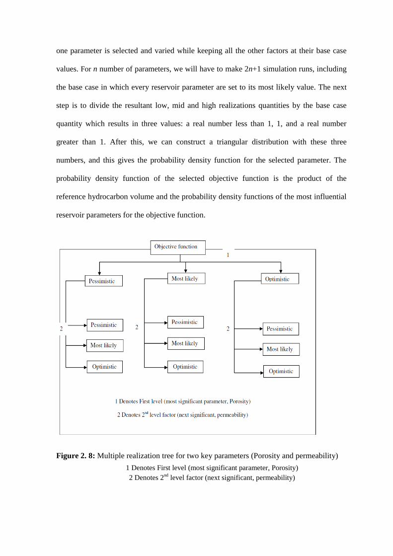
59
one parameter is selected and varied while keeping all the other factors at their base case
values. For n number of parameters, we will have to make 2n+1 simulation runs, including
the base case in which every reservoir parameter are set to its most likely value. The next
step is to divide the resultant low, mid and high realizations quantities by the base case
quantity which results in three values: a real number less than 1, 1, and a real number
greater than 1. After this, we can construct a triangular distribution with these three
numbers, and this gives the probability density function for the selected parameter. The
probability density function of the selected objective function is the product of the
reference hydrocarbon volume and the probability density functions of the most influential
reservoir parameters for the objective function.
Figure 2. 8: Multiple realization tree for two key parameters (Porosity and permeability)
1 Denotes First level (most significant parameter, Porosity)
2 Denotes 2nd
level factor (next significant, permeability)

60
This is obtained using Monte Carlo simulation. For illustration, if we consider OGIP as the
objective function, using this method the expression for MCS is given as:
OGIP = OGIPbase case ∗ ∆1 ∗ ∆2 ∗ … ∗ ∆n 2.47
Where n is the distribution of the hydrocarbon volume; OGIPbase case is the value of the
hydrocarbon volume for the base case; Δ is the distribution of the variation factors for the
identified key parameters that affect the OGIP. The advantage of this method is that it
requires fewer number of simulation runs for instance, if the identified number of key
factors is 8, the maximum number of simulation runs to be made is 17. This is much lower
when compare with experimental design or realization tree methods. The limitation of this
approach is that it ignores the effect of factor interactions.
2.8.4 Bayesian approach
Bayes’ theorem can be used in many applications in which we need to access the
probabilities of the causes. The method has been applied in uncertainty analysis in the
petroleum industry for some years (Barker et al., 2001). The philosophy is based on
theorem from probability theory first proposed in the eighteenth-century by Thomas Bayes.
A brief illustration of the theorem is to assume B1, B2… Bn to be n mutually exclusive
outcomes of some event B. if we let A (A is not perfect information; it simply correlated to
the event B, otherwise, Bayes’ theorem is not needed) be an outcome of an “information”
or a “symptom” related to B.
Then,

61
P(Bi
A⁄ ) =P (A Bi
⁄ ) P(Bi)
∑ P (A Bj⁄ ) P(Bj)
kj=1
2.48
𝑤ℎ𝑒𝑟𝑒 𝑖 = 1,2,3… . . 𝑘
P (A / Bi) is the conditional probability of event A occurs when Bi event has happened.
P (Bi) and P (Bj) are respectively the probability of events Bi and Bj
P (Bi/A) is called the probability of the causes.
Scales and Snieder, (1997) explained the use of Bayes’ theorem with this illustration thus
if suppose by previous work we know something about a model before using available data
(the prior knowledge and conjectures are called the a priori model), this knowledge is
transformed into likelihoods or probabilities. Often probabilities are assumed to follow a
Gaussian distribution. Suppose we then have a set of data with their variance and
covariance, Bayesian approach provides a method to fine-tune the a priori model with the
set of available data. The posterior distribution tells us how the data correct the prior
knowledge.
2.9 Overview of infill drilling
Infill drilling is one of the reservoir development concept usually implemented to recover
residual oil saturation. The determination of the amount of residual oil saturation after
primary and secondary recovery processes has been a challenge. Locating the oil to be
recovered is a difficult exercise and requires sophisticated techniques. Egbogah provided
extensive review of those techniques (Egbogah, 1994). Volumetric reservoir engineering

62
studies and core analysis can indicate amount of the remaining oil but not the distribution
of it. Tracer tests or well test methods are used to determine the location and distribution of
the oil remained. Table 2. 5 shows a brief review of some of the techniques used to
determine the amount of remaining oil.
The success of infill drilling as pointed out by Subbey et al., (2003) and Bustamante et al.,
(2005), is directly related to the uncertainties associated with it. Individual reservoir
characteristics all add up to give a resultant total uncertainty associated with reservoir
performance. Analytical models are characterized by several assumptions and are
becoming less efficient in estimation and quantification of various uncertainties due to
increasing complexity of petroleum reservoirs.
According to Ofoh, (1992), infill drilling can improve the recovery of hydrocarbon by
accelerating the hydrocarbon productions. However, the determination of infill potential as
well as selection of well type and placement has been a challenge (Thakur et al., 1998).
The recommended way to determine infill-drilling potential in a reservoir is to conduct a
complete reservoir evaluation involving geological, geophysical, and reservoir analyses
and interpretations. This approach is prohibitively time-consuming and expensive for some
large hydrocarbon fields (Linhua et al., 2005). Infill Drilling Predictive Model (IDPM)
which requires minimum amount of reservoir and geologic description has also been used
(Fuller et al., 1992). However, IDPM requires knowledge of heterogeneity elements (pay
continuity and permeability variation among layers.) which are not easily or often
measured in actual fields. Voneiff and Cipolla, (1996) developed a model-based analysis
method, the moving window technique, and apply it for rapid assessment of infill and re-

63
completion potential in the Ozona field. The method according to the author is quick but
the accuracy decreases with increasing heterogeneity. Empirical correlations (Hudson et
al., 2000) are also available to determine infill potential in a complex, low-permeability
gas reservoir. These correlations are reservoir specific and therefore have gained limited
applications. The use of numerical-based instead of analytical based conceptual models
has been reported (Pathak et al., 2000).
Table 2. 5: Summary of correlations for determination of residual oil saturation
Methods References Correlations
Core residual oil
saturation
(Kazemi, 1977) (𝑆𝑜 )𝑟𝑒𝑠 = (𝑆)𝑐𝑜𝑟𝑒𝐵𝑜𝐸
𝑀
1 − 𝑉2
Logs
Waxman and Thomas,
1968
𝑆𝑤 =
[ 𝑅𝑜
𝑅𝑡(
1 + 𝑅𝑤𝐵𝑄𝑣
1 +𝑅𝑤𝐵𝑄𝑣
𝑆𝑤
)
1𝑛
]
Volumetric-Reservoir
Engineering
𝑆𝑜𝑟 =
(𝑁 − 𝑁𝑝)𝐵𝑜𝑊𝐹
7758𝐴𝐻∅
Production data
Arps, 1995 and
Fetkovich, 1987 𝑆𝑜 =
𝑉𝑜
𝑉𝑝
=(𝑁𝑓𝑜𝑖 − 𝑁𝑝)𝐵𝑜
𝑁𝑓𝑜𝑖𝐵𝑜𝑖(1 − 𝑐𝑓∆𝑃)/(1 − 𝑆𝑤𝑖)
Well Testing
Ramey, 1975 𝑆𝑜 =𝑐𝑡 − 𝑐𝑤 − 𝑐𝑓
𝑐𝑜 − 𝑐𝑤
Chemical Tracer
Tomich et al., 1973 𝑉𝑖 =
(1 − 𝑆𝑜)𝑉𝑊 + 𝐾𝑖𝑆𝑜𝑉𝑜(1 − 𝑆𝑜) + 𝐾𝑖𝑆𝑜
Log-inject-log
Verma et al., 1991 𝑆𝑂𝑅𝑊 =
0.06(1 − 𝑆𝑤)
∅

64
Conceptualized models have been used to provide answers to frequently asked questions
such as the numbers of wells and their optimum placement within the reservoir (Ogbe et
al., 2009). In this study, full field numerical simulation approach was used to evaluate infill
location, selection and placement.The study utilized pressure and saturation maps to
determine infill well locations within the reservoir sub-regions.

65
Chapter 3
3. Stochastic Modeling
3.1 Problem Description
In this case study, the STOIIP was earlier estimated as 27 million stock tank barrels.
However, the analysis of production performance after fifteen years indicated a recovery
factor of approximately 40% for a reservoir under primary production scheme. It is
apparent from this figure that the reserve is under estimated. The main objective is to
determine realistic figure by revisiting the static model and assess associated uncertainty.
The Schlumberger- PETREL software was used for building the static model.
3.2 Static Modeling
To build the static model, the workflow shown in Figure 3. 1 was adopted. The
methodology involves data acquisition, quality checking, petrophysical analysis,
Geocellular modeling, and development of geological concept, property upscaling,
Variogram modeling, properties distribution, volume calculation and uncertainty
quantification.
3.2.1 Data acquisition and quality checking
Table 3. 1 shows all the available well logs in all the wells and includes lithology logs
(GR-log and SP), resistivity logs, density (RHOB), sonic logs and Neutron logs. Check
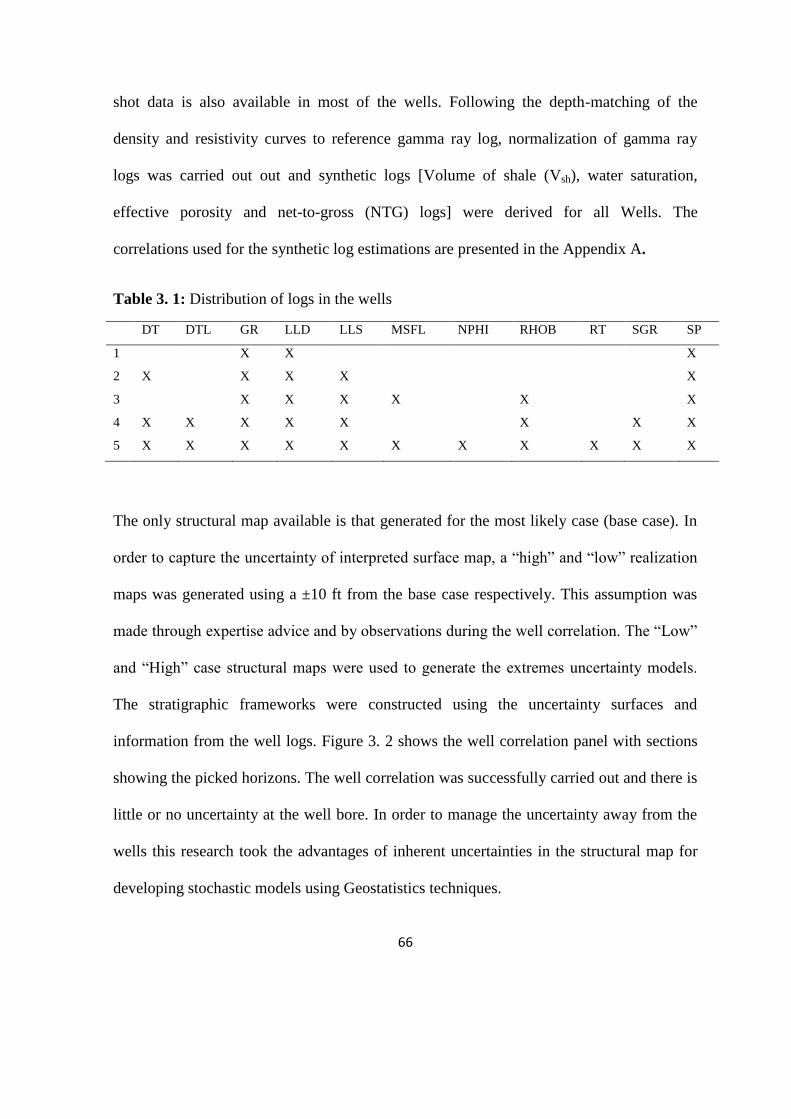
66
shot data is also available in most of the wells. Following the depth-matching of the
density and resistivity curves to reference gamma ray log, normalization of gamma ray
logs was carried out out and synthetic logs [Volume of shale (Vsh), water saturation,
effective porosity and net-to-gross (NTG) logs] were derived for all Wells. The
correlations used for the synthetic log estimations are presented in the Appendix A.
Table 3. 1: Distribution of logs in the wells
DT DTL GR LLD LLS MSFL NPHI RHOB RT SGR SP
1 X X X
2 X X X X X
3 X X X X X X
4 X X X X X X X X
5 X X X X X X X X X X X
The only structural map available is that generated for the most likely case (base case). In
order to capture the uncertainty of interpreted surface map, a “high” and “low” realization
maps was generated using a ±10 ft from the base case respectively. This assumption was
made through expertise advice and by observations during the well correlation. The “Low”
and “High” case structural maps were used to generate the extremes uncertainty models.
The stratigraphic frameworks were constructed using the uncertainty surfaces and
information from the well logs. Figure 3. 2 shows the well correlation panel with sections
showing the picked horizons. The well correlation was successfully carried out and there is
little or no uncertainty at the well bore. In order to manage the uncertainty away from the
wells this research took the advantages of inherent uncertainties in the structural map for
developing stochastic models using Geostatistics techniques.

67
Figure 3. 1: Workflow for Static and uncertainty Analysis
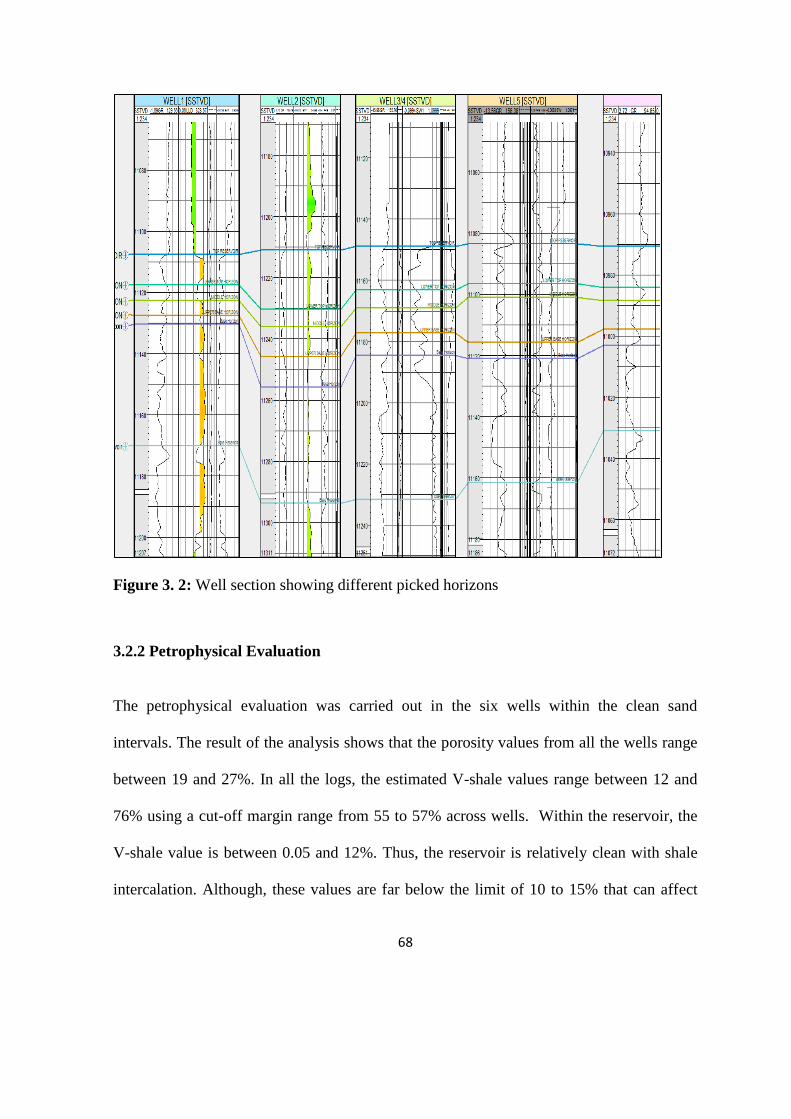
68
Figure 3. 2: Well section showing different picked horizons
3.2.2 Petrophysical Evaluation
The petrophysical evaluation was carried out in the six wells within the clean sand
intervals. The result of the analysis shows that the porosity values from all the wells range
between 19 and 27%. In all the logs, the estimated V-shale values range between 12 and
76% using a cut-off margin range from 55 to 57% across wells. Within the reservoir, the
V-shale value is between 0.05 and 12%. Thus, the reservoir is relatively clean with shale
intercalation. Although, these values are far below the limit of 10 to 15% that can affect

69
water saturation according to Hilchie, (1978), the fact that the sand is not completely clean,
it could affect the water saturation model. Thus, water saturation is one of the uncertainties
identified from this stage. The effective water saturation (Sw) was estimated using the
Indonesian model. The need to adequately condition the saturation log estimates to Vsh
informed the decision to select Indonesian correlation instead of Archie’s model. The
water resistivity was obtained using Pickett plot to be 4.2 Ωm while average shale
resistivity of 0.047 Ωm was obtained from the log. The obtained Sw average value of 19%
implies the occurrence of hydrocarbons within the sand intervals. The deep and shallow
resistivity logs indicated the presence of hydrocarbon within the sand while neutron-
density logs suggested that the fluid in the reservoir is oil.
3.2.3 Property cross-plots
Figure 3. 3 shows the graph of porosity versus Vsh. It is evident the existence of a strong
correlation between the porosity and Vsh. Porosity fitted well with Vsh using a polynomial
model with high correlation coefficient (R-square = 0.9). This value of R-square indicates
that the polynomial correlation can be used in the property distribution process with high
confidence. The downward sloping of the graph from left to right indicated that porosity is
negatively correlated with Vsh. This is expected within a hydrocarbon interval. It is also
evident from Figure 3. 3 that porosity values are more concentrated where the Vsh values
are smaller. Such interval could be very good for hydrocarbon storage if the water
saturation is small. This is generally true as shale formations are characterized by a low
porosity values. The scatter plot of porosity and permeability in Figure 3. 4 shows non-
linear correlation between the two properties.

70
Figure 3. 3: Scatter plot of Porosity versus Volume of shale (Vsh)
Figure 3. 4: Scatter plot of permeability versus porosity
y = -0.0287x2 - 0.1488x + 0.2756 R² = 0.9
0.15
0.17
0.19
0.21
0.23
0.25
0.27
0.05 0.25 0.45 0.65
Poro
sity
Vsh
y = 127.65e17.095x R² = 0.9161
1
10
100
1000
10000
100000
0 0.1 0.2 0.3 0.4
Per
mx
(m
d)
Porosity (%)

71
However, porosity varied positively with logarithm of permeability. As the porosity
increases, the permeability also increases. The model equation is displayed on the graph
with high correlation coefficient of correlation (R-square = 0.92). The coefficient as high
as this value indicated that such model equation can be employed for property distribution
if adequately constrained with other properties.
3.3 Construction of Geocellular Models
The Geocellular frameworks were constructed with a commercial reservoir simulator using
32,634 grid blocks. The cell size (ΔX*ΔY*ΔZ) used is 50 m x 50 m x1ft which was
believed to have captured all the intra-reservoir heterogeneities. In order to manage the
uncertainty away from the wells, Variogram models were built for all the properties from
well log. Property estimation was done using kriging and Sequential Gaussian Simulation
methods as described in section 3.3.1.
3.3.1 Property distribution
The methodology adopted for the distribution of the various petrophysical properties
comprises of four major steps:
Step 1: Development of a geological concept:
This involved building of horizontal trend maps for all the Para-sequences that made up the
reservoir. The reason was to establish how shale volume trends within the reservoir. The
ultimate reason that necessitates this was due to lack of facies model or information from
where this could be modeled. It was therefore conceived that developing characteristic
trends for shale volume at different layers of the reservoir, the distribution can be used to
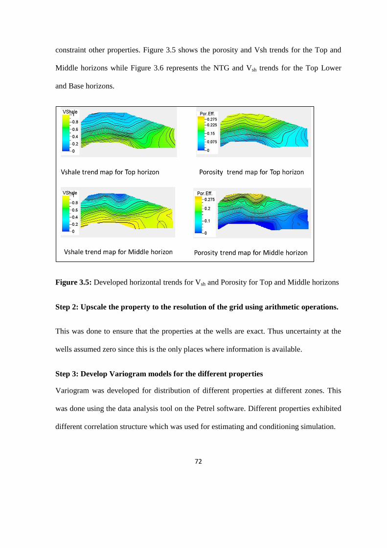
72
constraint other properties. Figure 3.5 shows the porosity and Vsh trends for the Top and
Middle horizons while Figure 3.6 represents the NTG and Vsh trends for the Top Lower
and Base horizons.
Figure 3.5: Developed horizontal trends for Vsh and Porosity for Top and Middle horizons
Step 2: Upscale the property to the resolution of the grid using arithmetic operations.
This was done to ensure that the properties at the wells are exact. Thus uncertainty at the
wells assumed zero since this is the only places where information is available.
Step 3: Develop Variogram models for the different properties
Variogram was developed for distribution of different properties at different zones. This
was done using the data analysis tool on the Petrel software. Different properties exhibited
different correlation structure which was used for estimating and conditioning simulation.
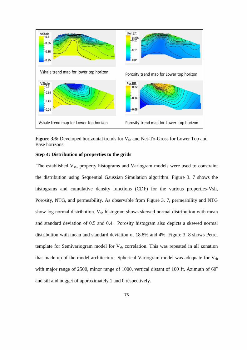
73
Figure 3.6: Developed horizontal trends for Vsh and Net-To-Gross for Lower Top and
Base horizons
Step 4: Distribution of properties to the grids
The established Vsh, property histograms and Variogram models were used to constraint
the distribution using Sequential Gaussian Simulation algorithm. Figure 3. 7 shows the
histograms and cumulative density functions (CDF) for the various properties-Vsh,
Porosity, NTG, and permeability. As observable from Figure 3. 7, permeability and NTG
show log normal distribution. Vsh histogram shows skewed normal distribution with mean
and standard deviation of 0.5 and 0.4. Porosity histogram also depicts a skewed normal
distribution with mean and standard deviation of 18.8% and 4%. Figure 3. 8 shows Petrel
template for Semivariogram model for Vsh correlation. This was repeated in all zonation
that made up of the model architecture. Spherical Variogram model was adequate for Vsh
with major range of 2500, minor range of 1000, vertical distant of 100 ft, Azimuth of 60o
and sill and nugget of approximately 1 and 0 respectively.
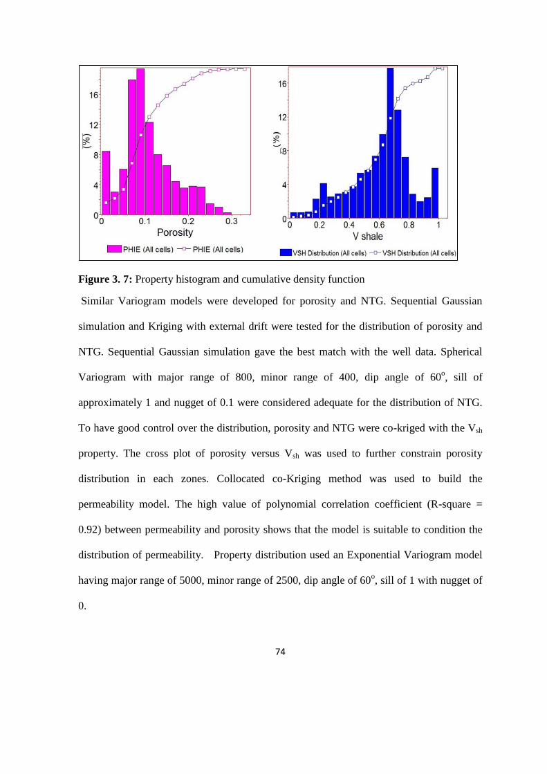
74
Figure 3. 7: Property histogram and cumulative density function
Similar Variogram models were developed for porosity and NTG. Sequential Gaussian
simulation and Kriging with external drift were tested for the distribution of porosity and
NTG. Sequential Gaussian simulation gave the best match with the well data. Spherical
Variogram with major range of 800, minor range of 400, dip angle of 60o, sill of
approximately 1 and nugget of 0.1 were considered adequate for the distribution of NTG.
To have good control over the distribution, porosity and NTG were co-kriged with the Vsh
property. The cross plot of porosity versus Vsh was used to further constrain porosity
distribution in each zones. Collocated co-Kriging method was used to build the
permeability model. The high value of polynomial correlation coefficient (R-square =
0.92) between permeability and porosity shows that the model is suitable to condition the
distribution of permeability. Property distribution used an Exponential Variogram model
having major range of 5000, minor range of 2500, dip angle of 60o, sill of 1 with nugget of
0.
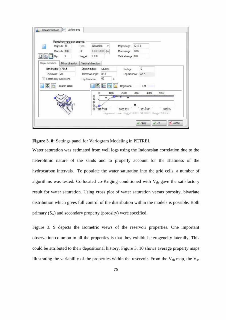
75
Figure 3. 8: Settings panel for Variogram Modeling in PETREL
Water saturation was estimated from well logs using the Indonesian correlation due to the
heterolithic nature of the sands and to properly account for the shaliness of the
hydrocarbon intervals. To populate the water saturation into the grid cells, a number of
algorithms was tested. Collocated co-Kriging conditioned with Vsh gave the satisfactory
result for water saturation. Using cross plot of water saturation versus porosity, bivariate
distribution which gives full control of the distribution within the models is possible. Both
primary (Sw) and secondary property (porosity) were specified.
Figure 3. 9 depicts the isometric views of the reservoir properties. One important
observation common to all the properties is that they exhibit heterogeneity laterally. This
could be attributed to their depositional history. Figure 3. 10 shows average property maps
illustrating the variability of the properties within the reservoir. From the Vsh map, the Vsh

76
distribution shows that shale volume increases from North to South. At the crest of the
structure where the wells are located, the Vsh ranges between 0 and 10% which justified the
location of the drainage points. This value increases down the structure both to the East
and West up to a maximum Vsh value of 75%.
Figure 3. 9: Isometric View of the Reservoir Properties
The water saturation map shows increasing water saturation from the North towards the
South. The minimum water saturation of 19.2% was found at the crest of the structure
while saturation as high as 67% occurs in the South. Both porosity and Net-To-Gross
properties show high values in the upper structure and decrease from North to South.
Permeability distribution is similar to the porosity distribution with minimum and
maximum values of 13 mD and 2154 mD, respectively in the models.

77
Figure 3. 10: Average Property Maps
Figure 3. 11, Figure 3. 12 and Figure 3. 13 show the distribution of Vsh, porosity, Net-To-
Gross and horizontal permeability in Layers 1, 3 and 5, respectively. All the properties
exhibit high level of variability across the layers. A lateral continuity that can be attributed
to the presence of stacked sandstone beds that are laterally continuous typical of a shore
face environment was observed. Although, Facies model was not generated for this study,
owing to the fact that core information was not available for supervision of the facies
distribution as at the time of carrying out this study, all distributions were conditioned to
Vsh following our developed sedimentological concept.

78
Figure 3. 11: Property distribution in the Layer 1
Figure 3. 12: Property distribution in the Layer 3

79
Figure 3. 13: Property distribution in the Layer 5
We recognized uncertainties in these models especially in the permeability distributions
that we assumed to be horizontally isotropic which may not reflect the actual local spatial
distribution of permeability. This drawback may affect the predictions as permeability has
a major effect on the fluid flow according to Kupfersberger and Deutsch, 1999.
3.3.2 Oil-In-Place Estimation and Uncertainty Quantification
A set of volumetric uncertainties, “low”, “mid” and “high” were calculated from the
“Low”, “Mid” and “High” case models. The uncertainty models were combined with the
hydrocarbon contact to arrive at the volumes that captured the range of uncertainties. The
formation volume factor (Boi) was derived from PVT analysis to be 1.25Scf/STB. Table 3.
2 shows some important uncertainty quantities obtained from the three models which
depict a marked difference in the reservoir pore volume, net volume, and bulk volume and
the STOIIP.
80
Table 3. 2: Deterministic Volumetric Uncertainties
Cases Pore Vol (RB) Net Vol (bbl) Bulk Vol (bbl) STOIIP (STB)
High 123 742 2017 55
Mid 117 666 2015 53
Low 116 663 2017 50
Average 118.7 690.3 2016.3 54
3.4 Volumetric Uncertainty Quantification
3.4.1 Uncertainty factors and their ranges
Uncertainty analysis was quantified on STOIIP using the ‘Low’, ‘Mid’ and ‘High’ case
static models. They were treated independently to represent low, mid and high ranges of
uncertain structural factor in an experimental design. In coded form, similar to other
parameters, the low, mid and high case models are denoted by (-1), (0) and (1)
respectively.
The main uncertainties affecting the evaluation of STOIIP for the reservoir are as follows:
i. Porosity
ii. Hydrocarbon saturation
iii. Net-to-Gross
iv. Oil Water Contact
v. Thickness

81
The selection of the multipliers for the ranges of uncertainties conforms to the practice in
the Niger Delta fields. This requires using 5-10% uncertainties on the hydrocarbon
saturation, 1-10% on porosity, 1-5 meters on hydrocarbon contacts, 5-10% on reservoir
NTG. Table 3. 3 shows various factors and range of parameters.
Table 3. 3: Uncertainty and their range of Multipliers
Uncertainty Units Low
High
PHIE fraction 0.9 1.1
Sw fraction 0.9 1.1
NTG fraction 0.9 1.1
OWC ft 0.9 1.1
Thickness ft -10 +10
3.4.2 Design of experiment
Table 3. 4 shows the CCD matrix used to conduct the experiment in coded form. Fifty (50)
experiments at various conditions were performed (see Appendix C3). The choice of CCD
was based on the need for accurate proxy model for the Monte Carlo. CCD, unlike other
response surface models, allows changing parameters at 5 levels (-α, -1, 0, 1, +α). The
design matrix consists of 42 non center factorial designs with the corners at ±1 of the cube,
augmented by additional “star” and eight rotatable “center” points (±α), which allow the
estimation of the second order polynomial equation. The data set was partitioned into two,
40 data set were used for model building while the remaining data was used for validation.
In order to study the effects of the main variables and possibly the interaction effects of the

82
identified uncertainties, the significance of the various parameters was determined using
Analysis of Variance (ANOVA). This was done by rejecting null hypothesis.
Table 3. 4: Experimental Design Matrix (CCD)
Run PHIE SW NTG OWC
Thicknes
s Run PHIE SW NTG OWC
Thicknes
s
1 1 -1 1 1 -1 26 1 1 -1 1 -1
2 -1 -1 1 -1 1 27 1 -1 1 -1 1
3 0 0 0 0 0 28 -1 1 -1 -1 1
4 0 0 0 0 0 29 0 0 2 0 0
5 2 0 0 0 0 30 0 0 0 0 0
6 1 1 -1 -1 -1 31 1 1 1 1 -1
7 -1 1 1 1 1 32 1 1 1 1 1
8 -2 0 0 0 0 33 -1 -1 -1 -1 -1
9 0 0 0 0 2 34 0 0 0 0 0
10 1 -1 -1 -1 -1 35 1 1 -1 -1 1
11 1 -1 1 1 1 36 1 1 -1 1 1
12 -1 -1 1 1 1 37 -1 1 -1 -1 -1
13 -1 1 -1 1 1 38 0 2 0 0 0
14 0 -2 0 0 0 39 0 0 0 0 -2
15 0 0 0 0 0 40 -1 1 -1 1 -1
16 0 0 0 0 0 41 -1 -1 -1 -1 1
17 -1 -1 -1 1 -1 42 1 -1 -1 1 -1
18 0 0 0 0 0 43 -1 -1 -1 1 1
19 -1 1 1 -1 -1 44 1 -1 -1 1 1
20 -1 -1 1 1 -1 45 1 1 1 -1 1
21 1 -1 1 -1 -1 46 1 -1 -1 -1 1
22 0 0 0 -2 0 47 0 0 0 2 0
23 1 1 1 -1 -1 48 -1 1 1 1 -1
24 0 0 0 0 0 49 -1 1 1 -1 1
25 -1 -1 1 -1 -1 50 0 0 -2 0 0

83
3.4.3 Analysis of variance
To determine whether there is a linear relationship between the response and various
factors, test for significance of regression was performed by Analysis of Variance. Fisher
variable (F) and its associated probability (prob>F) was used to assess the model
significance and to select regressors with high impact on the model. A 95% confidence
level (i.e. α = 0.05) was assumed for the analysis. Table 3. 5 is ANOVA for CCD. The
Model F-value of 149.28 implies the model is significant. The p-value obtained implies
that there is only a 0.01% chance that a "Model F-Value" this large could occur due to
noise. Values of "Prob > F" less than 0.0500 indicate models terms are significant. In this
case main factors PORO, SW, NTG, OWC and thickness are all significant model terms.
Also, some significant interaction terms include PORO*OWC, PORO*NTG and
NTG*OWC. With the combination of these factors, the final proxy model developed is:
𝑆𝑇𝑂𝐼𝐼𝑃 (𝑀𝑀𝑆𝑇𝐵) = 5558.31582 − 5159.61258 ∗ 𝑃𝑂𝑅𝑂 − 3.01510 ∗ 𝑆𝑊 −
3758.42013 ∗ 𝑁𝑇𝐺 − 0.49283 ∗ 𝑂𝑊𝐶 − 0.057327 ∗ 𝑡ℎ𝑖𝑐𝑘𝑛𝑒𝑠𝑠 + 70.78169 ∗ 𝑃𝑂𝑅𝑂 ∗
𝑁𝑇𝐺 + 0.45782 ∗ 𝑃𝑂𝑅𝑂 ∗ 𝑂𝑊𝐶 + 0.33282 ∗ 𝑁𝑇𝐺 ∗ 𝑂𝑊𝐶 3.1
Using this model, the mean estimated STOIIP is 53.33 MMSTB. This figure approximates
the experimental value of 55 MMSTB with standard deviation of 1.13, covariance of 2.1
and adequate precision of 66 (value > 4 is desirable).

84
Table 3. 5: Analysis of Variance for STOIIP
Source
Sum of
Squares DF
Mean
Square F Value Prob > F
Model 1523.24 8 190.41 149.28 < 0.0001
PORO 750.79 1 750.79 588.61 < 0.0001
SW 3.56 1 3.56 2.79 0.01041
NTG 813.59 1 813.59 637.85 < 0.0001
OWC 336.16 1 336.16 263.54 < 0.0001
Thickness 10.43 1 10.43 8.18 0.0073
PORO*NTG 12.84 1 12.84 10.06 0.0033
PORO*OWC 5.37 1 5.37 4.21 0.0482
NTG*OWC 2.84 1 2.84 2.23 0.1453
Residual 42.09 33 1.28
Lack of Fit 42.09 26 1.62
Pure Error 0 7 0
Cor Total 1565.33 41
3.4.4 Model Validation
Figure 3. 14 shows the cross plot of the actual experimental values against the predicted
values. Also on the same graph is the plot of the validation. The alignment of the values to
the 45o line shows that the model is predictive in nature. The maximum error (equation
3.2) recorded for the validation using developed model was 6%. The high correlation
coefficients obtained (R-square = 0.97, Adj. R-square = 0.97 and prediction R-square =
0.96) show that the model terms are significant and overall, the model is reliable and can
be used to sample the space within the uncertainty ranges. This equation can therefore be
applied for uncertainty quantification.

85
𝐸𝑚𝑎𝑥 = 𝑀𝐴𝑋𝐼=1𝑛 |𝐸𝑖| 3.2
Where,
𝐸𝑖 = | 𝑀𝑒𝑎𝑠𝑢𝑟𝑒𝑑 − 𝑃𝑟𝑒𝑑𝑖𝑐𝑡𝑒𝑑
𝑃𝑟𝑒𝑑𝑖𝑐𝑡𝑒𝑑|𝑖∗ 100
Figure 3. 14: Parity plot showing the cross actual values against the predicted value
3.5 Uncertainty Quantification
Linear, perturbation, and the scenario creation approach are some of the available methods
for quantifying uncertainty. Because these methods are faster and easier for uncertainty
quantification, they are commonly used. However, as these methods utilize a single
reservoir description model (RDM), they often underestimate the associated uncertainty.
30
40
50
60
70
80
90
100
30 40 50 60 70 80 90 100
Pre
dic
ted V
alue
Experimental value
Predicted Value
Validation
Linear (Predicted Value)

86
This study imposed probability distribution function and described the chance of obtaining
a parameter value on the proxy model (Eq. 3.1) developed. An experimental probability
distribution was first determined, thereafter, a theoretical distribution that would have
produced such a sampling distribution were determined. After the uncertainty associated
with each individual input parameter is determined by probability density function, they
are treated individually and transformed into a composite uncertainty associated with the
simulation model.
The relationship between the parameters was observed to be nonlinear so the interaction
between the individual inputs parameters was determined by ANOVA. The choice of
probability distribution for the input parameters was guided by histogram plots and
experience from the neighbouring field. Most of these uncertainties do not follow normal
distribution patterns. Rather, their logarithm is normally distributed and an estimation of
upside potential (10%), 50%, and downside risk (90%) was determined. Figure 3.6 shows
the summary of the simulation statistics. Figure 3. 15 is the Tornado chart showing the
degree to which various uncertainties impact the response (STOIIP). The impacts of the
main attributes on the response were observed with porosity having the maximum
influence. Porosity, NTG and OWC have positive influence on the response (STOIIP) with
porosity the biggest driver. Both water saturation and structural map have a negative
influence on the response. The combined effect of structural map on the estimated volume
is a negative one. The probability density function and the STOIIP cumulative distribution
curve are shown in Figure 3.15b. The results show that there exists 10% probability of
having mostly 59 MMbll, 50% chance of equalling or exceeding 53 MMbll and 90%
chance of having 47 MMbll of STOIIP.

87
Table 3. 6: Summary of Simulation Statistics
Name
STOIIP
(MMSTB) PORO SW NTG OWC Thickness
P10 47.091 0.919 0.654 0.919 11225.400 -8.501
P50 52.620 0.999 0.974 0.999 11231.000 0.000
P90 58.919 1.079 1.295 1.079 11236.500 7.999
Figure 3. 15: (a) Tornado chart showing impact of various parameters on STOIIP (b)
Probability and Cumulative Density for STOIIP

88
3.6 Summary
The objective was to develop static model and carry out the uncertainty analysis on the
volumes of hydrocarbon in place. The proposed methodology can be summarised as
follows:
i. Three (3) static reservoir models were built based on the uncertainty in the
structural map.
ii. Before the distribution of properties in the geological models, the study
developed sedimentological concept using the distribution of shale within the
formation. Geostatistical method was applied for property prediction away from
well. All the properties were constrained using the volume of shale, histograms
and properties cross plots to ensure geological consistency aerially and
vertically.
iii. To quantify uncertainty in hydrocarbon volume, CCD algorithm was used to
combine all uncertainties with each model treated as uncertainty.
iv. The reliability of the model was tested before subjected to Ordinary Monte
Carlo simulation. A good correlation coefficient between the actual response
and prediction (R-square = 0.97) testified to the accuracy and reliability of the
proxy model.
v. The result shows that the earlier estimation was underestimated and that there
exists 10% probability of having at most 59 MMbll, 50% chance of equalling or

89
exceeding 53 MMbll and 90% probability of having at least 47 MMbll of
STOIIP.
90
Chapter 4
4. History Matching and Uncertainty Analysis
This Chapter covers review and quality checking of available PVT and other dynamic data;
material balance analysis to evaluate the aquifer properties; preparation of input data to
initialize the simulation model; history matching to calibrate the dynamic model to field
production history; and prediction of reservoir production performance. The dynamic
model was built using exported properties from the static models in the chapter 3. Static
and dynamic properties were integrated then the model initialized to equilibrate to the
initial pressure and saturation conditions. The static models were validated by matching
historical pressures and saturations observed from the reservoir. The available production
data span between 1993 and 2006. The simulation of pressure and water cut was used as
the basis for validating the quality of the history match. Prediction runs were performed to
estimate reserves and generate production forecasts uncertainties for the three model cases
in order to estimate the ultimate oil recovery from the reservoir and provide proper
management concept for its optimum recovery.
4.1 Review of reservoir data
The reservoir was completed with four wells, all deviated; AK-01, AK-02, AK-03 and AK-
04. The oil is characterized by average API gravity of 35 oAPI and viscosity ranges
between 1-1.3cp. The initial pressure was given to be 4951 psia at reference depth of
11142 ft and reservoir average temperature is 170oF. Within the reservoir, porosity

91
averaged at 26% and average water saturation observed is 19.6%. None of the wells
encountered an oil-water contact. However, the deepest oil-down-to (ODT) was seen by
AK-02 at 11231 feet. Production started from the reservoir from AK-01 in November 1993
with an average oil rate of 1500 stb/day, GOR of 500 scf/stb, and a BS&W of 0.05%. AK-
02 was opened to production in May 1995, both AK-03 and AK-04 was completed in
August, 1995. A peak oil production of 5000 stb/d with a GOR of 620 Mscf/stb and a
BS&W of 0.13% was attained in the reservoir in November 1998. Subsequently, the
reservoir experienced a production decline with increasing BS&W and GOR. Due to
inactive water drive, pressure decline of approximately 28% was recorded at the end of
December 1998. Cumulative production from this reservoir as of December 2006 is 26
MMstb of oil, 30 Mscf of gas, and 2.1 MMstb of water.
Figure 4. 1 and Figure 4. 2 show the reservoir production performance and the cumulative
oil, water and gas production in the reservoir. The production performance indicates a
realistic trend in oil and water production. Due to gas metering issues in the facilities, it
was assumed that the gas volumes recorded had inherent errors. Hence, apart from the
primary phase (oil rate) that will be constrained in the saturation match, preference was
given to matching the water cut. The workflow adopted for history matching follows that
from Almeida et al., (2003). Saturation match took place after matching the pressure. This
involves changing one parameter-at-a-time. Uncertainty attributes were identified in the
course of sensitivity study and field water-cut and cumulative water production for the
period of 15 years was matched.
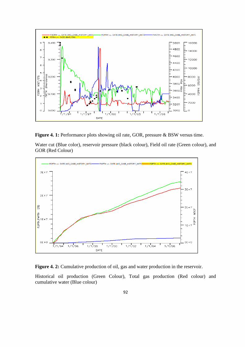
92
Figure 4. 1: Performance plots showing oil rate, GOR, pressure & BSW versus time.
Water cut (Blue color), reservoir pressure (black colour), Field oil rate (Green colour), and
GOR (Red Colour)
Figure 4. 2: Cumulative production of oil, gas and water production in the reservoir.
Historical oil production (Green Colour), Total gas production (Red colour) and
cumulative water (Blue colour)

93
4.2 Material Balance Analysis
4.2.1 Reservoir cross-sectional view
Figure 4. 3 is a cross section of the reservoir and shows the direction from where water
encroaches the reservoir. The direction of water influx was visualized and determined by
the relative positions of the oil water contact at different time. The positions of the OWC at
the start (November, 1993) and at the end (November, 2008) of the simulation have shown
that the left and right regions of the reservoir sections experienced water encroachment
earlier than the bottom, so the wells at the flanks experienced water influx earlier than
others. This shows the predominant of edge aquifer over the bottom.
4.2.2 Aquifer modelling
To model the aquifer and its characteristics, material balance calculation was made. The
aquifer was modelled using the Fetkovich analytical model. The choice of Fetkovich is
because it contains fewer parameters than others analytical models. The parameters in the
Fetkovich model are given in equations 4.1 through 4.3.
𝑊𝑖 =𝜋(𝑟𝑎
2 − 𝑟𝑟2)
5.615[
∅
360] 4.1
𝑟𝑎 = √43510𝐴𝑎
𝜋(360
∅) 4.2
𝐽 =0.00708𝑘ℎ (∅ 360⁄ )
𝜋 [𝑙𝑛 (𝑟𝑎𝑟𝑟
) − 0.75] 4.3

94
Figure 4. 3: Reservoir Cross section showing the aquifer movement
4.2.3 The analytical plot
The amount of the energy required to match the observed production was estimated
through the analytical plot by constraining the material balance model to produce the
observed pressure and the non-primary phases (gas and water) and then calculating the oil
production. As shown in Figure 4. 4, it is evident that without the presence of aquifer it is
impossible to match the observed pressure and then production.

95
Figure 4. 4: Analytical plot.
The red line represents material balance without aquifer while the blue trend line
represents that with the aquifer in place. With aquifer however, the energy was captured.
The discrete points represent the pressure history while the continuous lines (red and blue)
represent material balance results. To establish the aquifer properties, regression was done
and a match (blue line) was achieved in the analytical plot (reservoir pressure versus
cumulative oil production) as shown in Figure 4. 4.
With these details an estimate of the hydrocarbon zone to aquifer ratio was determined.
The aquifer estimated pore volume is approximately 3 MMMbbl and productivity index of
450 bll/psia/day. Other aquifer characteristics such as permeability, encroachment angle
and tank radius were also obtained. Below is the description of other important plots made
from the material balance calculations.

96
4.2.4 The aquifer influence functions (Wd)
The aquifer influence function is shown in Figure 4. 5. Wd plot is used to determine the
time the aquifer will respond to voidage due to fluid removal. It helps to determine the
ratio of the aquifer radius to the reservoir radius (aquifer size). For this reservoir, the
aquifer influence function revealed the ratio of the aquifer radius to the reservoir radius
(aquifer size) to be 6 which is an indication of appreciable aquifer which is likely to react
later to voidage caused by oil, water and gas production through the wells.
Figure 4. 5: Material balance Wd function plot
4.2.5 The reservoir drive mechanisms
Figure 4. 6 is the energy plot and it shows that the reservoir energy is majorly a
combination of water influx and pore volume expansion from the aquifer. Initially the fluid
expansion is the dominant energy source, but as reservoir depletion continuing, pore
volume expansion from the aquifer becomes more significant drive. Usually, with these
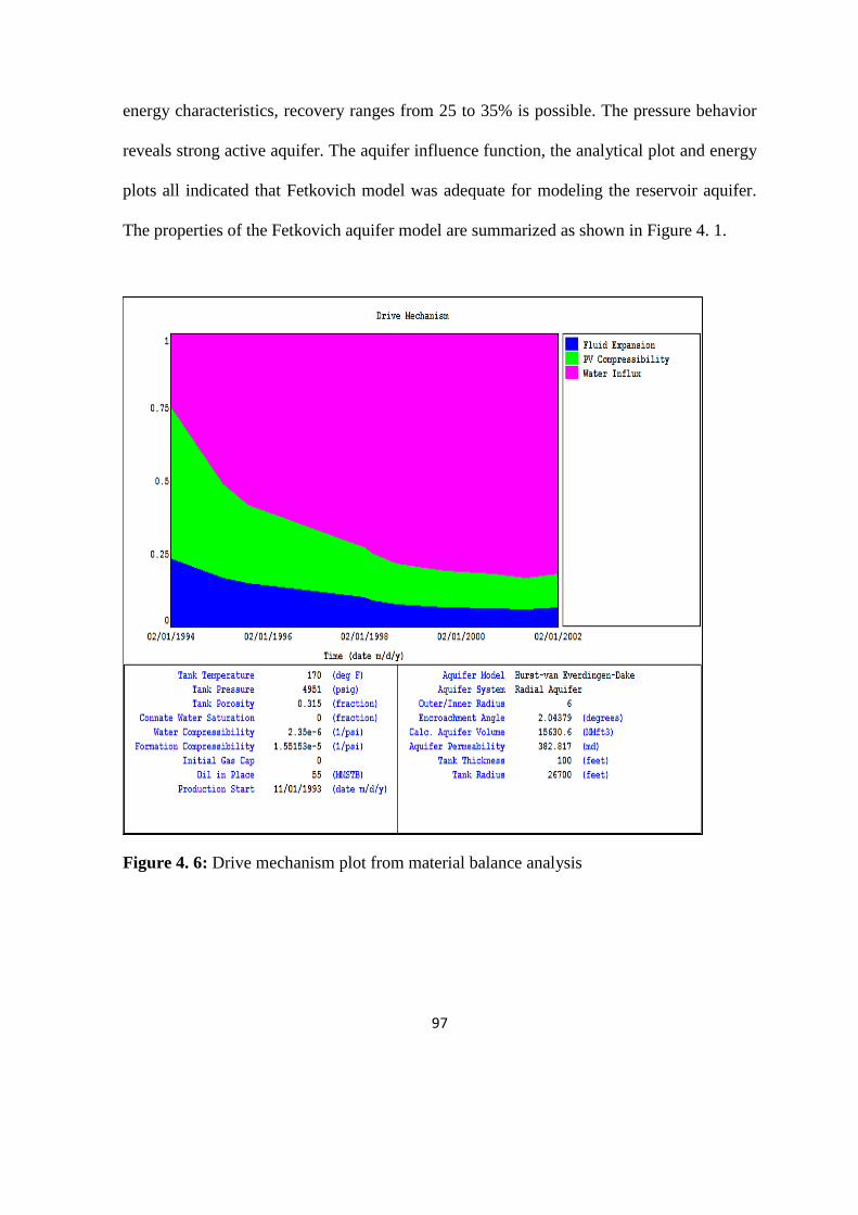
97
energy characteristics, recovery ranges from 25 to 35% is possible. The pressure behavior
reveals strong active aquifer. The aquifer influence function, the analytical plot and energy
plots all indicated that Fetkovich model was adequate for modeling the reservoir aquifer.
The properties of the Fetkovich aquifer model are summarized as shown in Figure 4. 1.
Figure 4. 6: Drive mechanism plot from material balance analysis

98
Table 4. 1: Aquifer properties for field pressure history match
Parameters Estimated values
Reservoir Outer/Inner radius 6
Permeability 382.817mD
Porosity 0.315
Compressibility 2.35E-06/psi
Aquifer Thickness 100ft
4.3 Dynamic Simulation
4.3.1 Model dimensions
The reservoir model was constructed using the data obtained from the static model,
material balance analysis and pertinent rock and fluid properties, SCAL, well completions
and production data. The model dimensions in the X-, Y- and Z-direction are 197, 75 and
9, respectively. This amounts to 132,975 active cells on a fine scale equivalent to 98*37*9
grid dimension (32,634 3D grid blocks) on a coarse scale. This was able to preserve certain
geologic features like thin shale streaks captured in certain layers of the geologic model.
4.3.2 Model properties
Properties used to build the dynamic model are as follows:
i. Permeability in the X and Y direction for all the cells (PERMX, PERMY)
ii. Permeability in the Z direction (PERMZ)
iii. Porosity (PHIE)
iv. Saturation model
v. Net to gross (NTG).

99
vi. SCAL data comprising the relative permeabilities for oil/water and gas/oil
systems
vii. PVT data.
4.3.3 Schedule
The production history and deviation survey for the wells were loaded into the simulation
model using ECLIPSE schedule. The program calculates the well connection factors using
the reservoir properties. In addition, the program outputs the production data in a format
that can be included directly into an ECLIPSE model.
4.4 Sensitivity Analysis
Traditional history match can be time consuming especially when huge uncertainties
influence reservoir performance of interest. Accurate identification of factors and their
interactions are difficult to achieve when parameters are changed one-at-a-time. Linear
experiments were therefore designed for screening 11 reservoir factors in order to identify
most impactful ones for the purpose of saturation match and uncertainty analysis.
The following factors were considered for sensitivity study on the 3 models:
i. Critical water saturation, (SWCR)
ii. Critical gas saturation (Sgc)
iii. Irreducible water saturation (SWI)
iv. Porosity (PORO)
v. Water relative permeability (KRW)

100
vi. Aquifer volume, (AQPV)
vii. Aquifer productivity index (AQUIPI)
viii. Vertical permeability, (KZ)
ix. Horizontal permeability, (KX)
x. Global fluid contact, (OWC)
xi. Oil viscosity, (µo)
4.4.1 Placket-Burman Design
Placket-Burman was chosen because it permits screening relatively large number of
parameters with minimum number of simulations. PB has a limitation of not been able to
account for higher order and interaction effects that may at times be significant.
Nevertheless, the objective at this stage is not seeking for “detail” nor for the development
of credible reservoir proxy, rather it is employed to identify major factors to focus attention
on while performing traditional history matching. This was performed on “High”, “Mid”
and “Low” case models. In all cases, cumulative oil produced was the response. Twelve
experiments were performed at various settings.
Table 4.2Table 4.2: shows the design levels for different parameters. All entries in the third
and fourth columns represent multiplier on the base case model. The definition of these
multipliers was based on expert advice and experience gained from the neighbouring
fields.
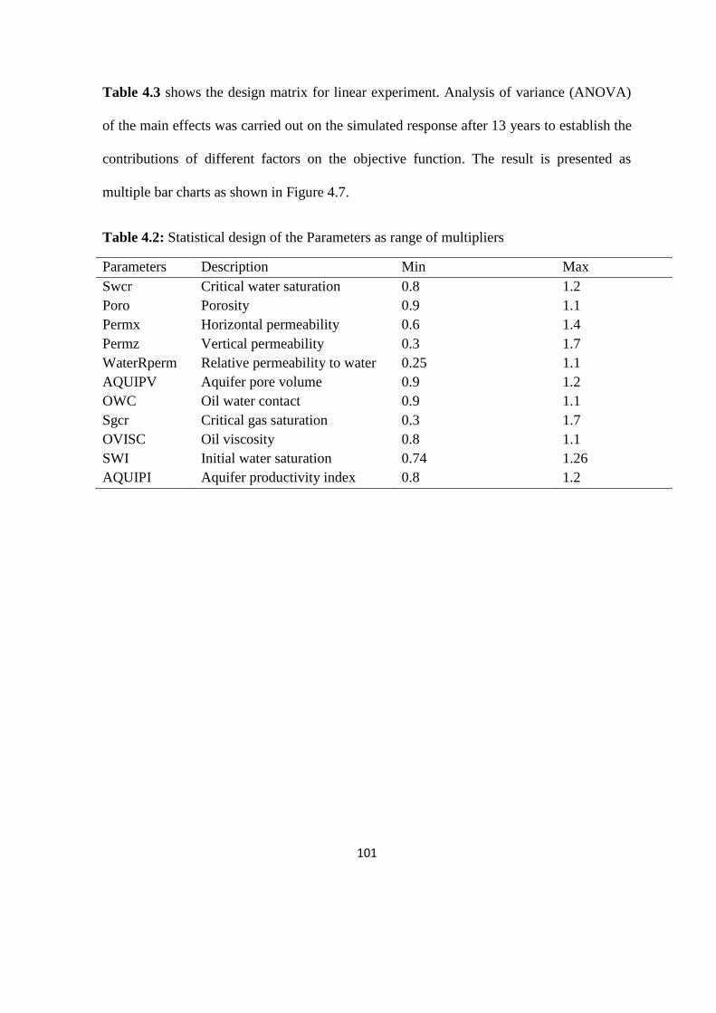
101
Table 4.3 shows the design matrix for linear experiment. Analysis of variance (ANOVA)
of the main effects was carried out on the simulated response after 13 years to establish the
contributions of different factors on the objective function. The result is presented as
multiple bar charts as shown in Figure 4.7.
Table 4.2: Statistical design of the Parameters as range of multipliers
Parameters Description Min Max
Swcr Critical water saturation 0.8 1.2
Poro Porosity 0.9 1.1
Permx Horizontal permeability 0.6 1.4
Permz Vertical permeability 0.3 1.7
WaterRperm Relative permeability to water 0.25 1.1
AQUIPV Aquifer pore volume 0.9 1.2
OWC Oil water contact 0.9 1.1
Sgcr Critical gas saturation 0.3 1.7
OVISC Oil viscosity 0.8 1.1
SWI Initial water saturation 0.74 1.26
AQUIPI Aquifer productivity index 0.8 1.2
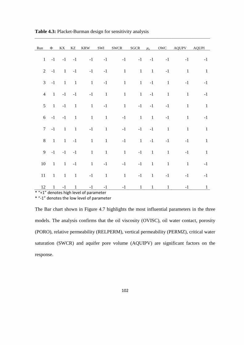
102
Table 4.3: Placket-Burman design for sensitivity analysis
Run Φ KX KZ KRW SWI SWCR SGCR 𝜇o OWC AQUPV AQUPI
1 -1 -1 -1 -1 -1 -1 -1 -1 -1 -1 -1
2 -1 1 -1 -1 -1 1 1 1 -1 1 1
3 -1 1 1 1 -1 1 1 -1 1 -1 -1
4 1 -1 -1 -1 1 1 1 -1 1 1 -1
5 1 -1 1 1 -1 1 -1 -1 -1 1 1
6 -1 -1 1 1 1 -1 1 1 -1 1 -1
7 -1 1 1 -1 1 -1 -1 -1 1 1 1
8 1 1 -1 1 1 -1 1 -1 -1 -1 1
9 -1 -1 -1 1 1 1 -1 1 1 -1 1
10 1 1 -1 1 -1 -1 -1 1 1 1 -1
11 1 1 1 -1 1 1 -1 1 -1 -1 -1
12 1 -1 1 -1 -1 -1 1 1 1 -1 1
* “+1” denotes high level of parameter * “-1” denotes the low level of parameter
The Bar chart shown in Figure 4.7 highlights the most influential parameters in the three
models. The analysis confirms that the oil viscosity (OVISC), oil water contact, porosity
(PORO), relative permeability (RELPERM), vertical permeability (PERMZ), critical water
saturation (SWCR) and aquifer pore volume (AQUIPV) are significant factors on the
response.

103
Figure 4. 7: Bar chart showing degree of significance of uncertainties from the three
models on response
4.5 Saturation Match
The simulator was constrained to produce the historical oil rates and then the water cut,
GOR and reservoir pressure were estimated. These were then compared to historical data
to validate the dynamic model. The following changes were made to the simulation model
to obtain a good history match of the pressure and production profiles:
Relative permeability to water
There was no relative permeability measurement available. The measurement from
analogous reservoir was utilized after modification. Keeping end points constant, a low and
high cases water relative permeability were derived from the initial assumed curves (mid
0.E+00
5.E+05
1.E+06
2.E+06
2.E+06
3.E+06
Coef
fici
ents
Parameters
LOW_CASE MODEL MID_CASE MODEL HIGH_CASE MODEL

104
case ) using some multipliers. By so doing the rock wettability become altered until
satisfactory match is obtained. The relative permeability plots for oil-water and gas-oil
systems used in this study are shown in Figure 4. 8 and Figure 4. 9. The connate water
saturations obtained from the static model were relatively low. Critical water saturation
was globally increased by 25% to match the water breakthrough time.
Figure 4. 8: Oil-water relative permeability curves
Oil Viscosity
The key oil properties available after carefully reviewed the PVT and sampling depth data
for this reservoir include; gas-oil-ratio (GOR), gas gravity, oil API gravity and oil
formation volume factor (FVF). Empirical correlation was used for oil viscosity and other
PVT properties estimation. So, uncertainty of ±10% was assumed for the resulted single
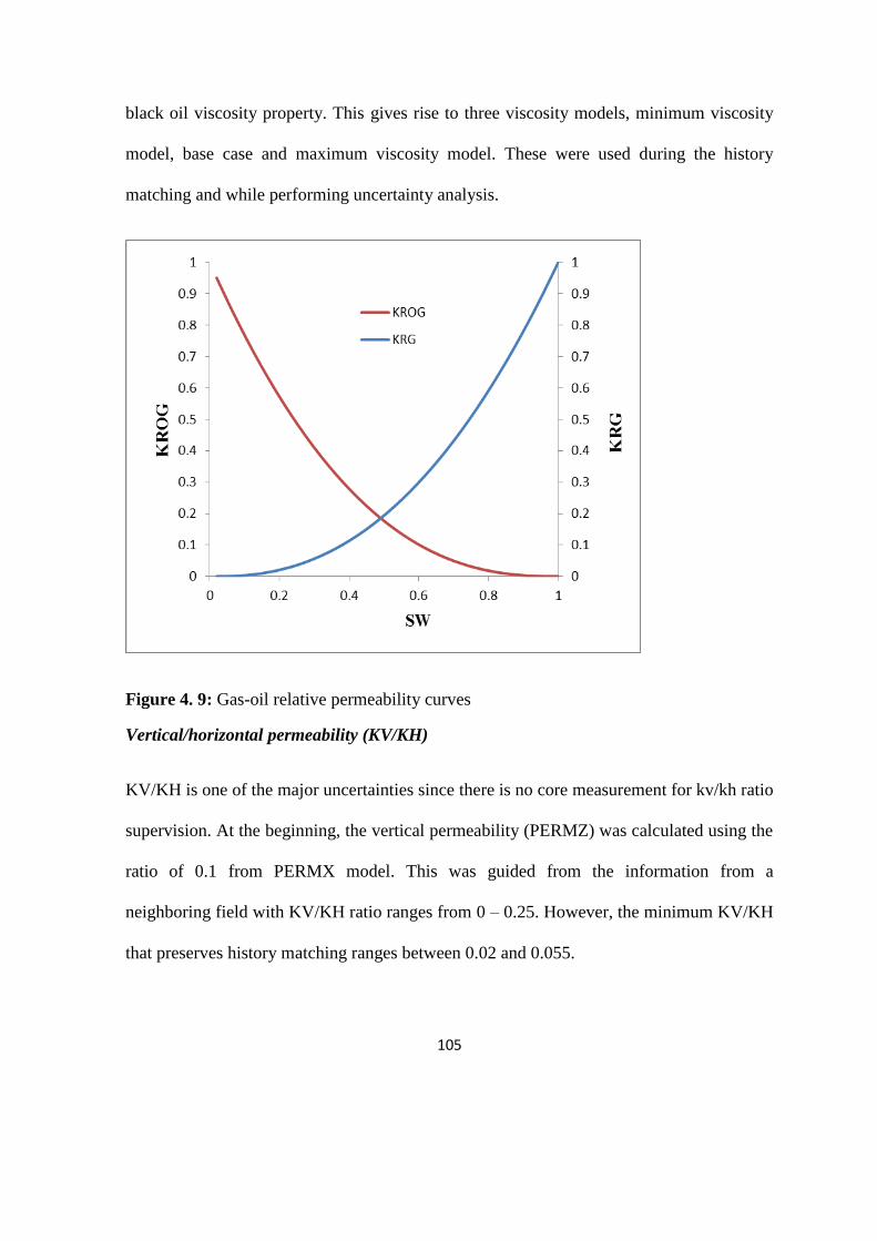
105
black oil viscosity property. This gives rise to three viscosity models, minimum viscosity
model, base case and maximum viscosity model. These were used during the history
matching and while performing uncertainty analysis.
Figure 4. 9: Gas-oil relative permeability curves
Vertical/horizontal permeability (KV/KH)
KV/KH is one of the major uncertainties since there is no core measurement for kv/kh ratio
supervision. At the beginning, the vertical permeability (PERMZ) was calculated using the
ratio of 0.1 from PERMX model. This was guided from the information from a
neighboring field with KV/KH ratio ranges from 0 – 0.25. However, the minimum KV/KH
that preserves history matching ranges between 0.02 and 0.055.

106
Original Oil-Water Contact (OWC
The first well drilled in 1973 penetrated the sand without encountered the water-up-to
(WUP) depth. However, the water-up-to from two simultaneously drilled wells indicated
slightly varying depths. The average Oil-Down-To (ODT) from these wells is
approximately 11239 TVD ftss. The base case match was obtained using 11240.5TVD ftss,
for the low case model, a good match was obtained with ODT at 11245.5TVD ftss while
for the high case, the ODT at 11238TVD ftss was adequate to obtain a good pressure and
saturation matches.
A good match on water cut and pressure was obtained at reservoir level. Figure 4. 10,
Figure 4. 11 and Figure 4. 12 show the outcome of the history match. This results in
complimentary good match in the oil volume and oil rate. Although the water
breakthrough time for high case was early than actual observed, the overall water cut
match, though characterized with little variation in levels for the three cases, are relatively
good.
4.5 Prediction
The objective of the prediction runs is to generate production forecasts uncertainties from
the models and evaluate possible field development cases in order to optimize oil recovery
from the reservoir. The current potential of the wells was evaluated and this formed the
basis for defining the individual well production rate constraints. Forecast period assumed
is 15 years.

107
Table 4.4 shows the operational and economic constraints applied to the producing wells
during the prediction runs.
Figure 4. 10: History match plots Reservoir pressure, GOR, oil rate and water cut for Base
case model

108
Figure 4. 11: History match plots Reservoir pressure, GOR, oil rate and water cut for Low
case model

109
Figure 4. 12: History match plots Reservoir pressure, GOR, oil rate and water cut for High
case model

110
Table 4.4: Producing constraints
Constraints Low case Base case High case
Minimum oil rate (stb/d) 500 500 500
Maximum GOR (scf/ stb) 850 850 850
Maximum BS&W (Percent) 90 90 90
Maximum oil rate (stb/d) 2000 2000 2000
The following case scenario was evaluated:
CASE 1: Do nothing Case
Prediction for do nothing cases using “high”, “low” and “mid” case models were
performed assuming that the existing wells AK-01, AK-03, AK-05 and AK-06 will
continue to produce without any intervention. Two of the wells, AK-01 and AK-03,
stopped production prior to the end of history owing to excessive water production. The
production performance plots for the reservoir under this condition are shown in Figure 4.
13 and Figure 4. 14. It is obvious in Figure 4. 14 that well AK-06 is making more water
than AK-05. However, in all wells the high case model produced less water and hence high
oil production. The base case yielded an estimated cumulative oil recovery of 31 MMstb.
The well AK-06 from shuts down barely eight years into the prediction phase. Overall, the
reservoir can still produce additional 6.3 MMstb of oil from July 2007 until 2020.
CASE 2: Pressure Maintenance and Well intervention
The second management case involved pressure maintenance by water injection and
intervention in well AK-06 based on its completion’s water production exceeding specified
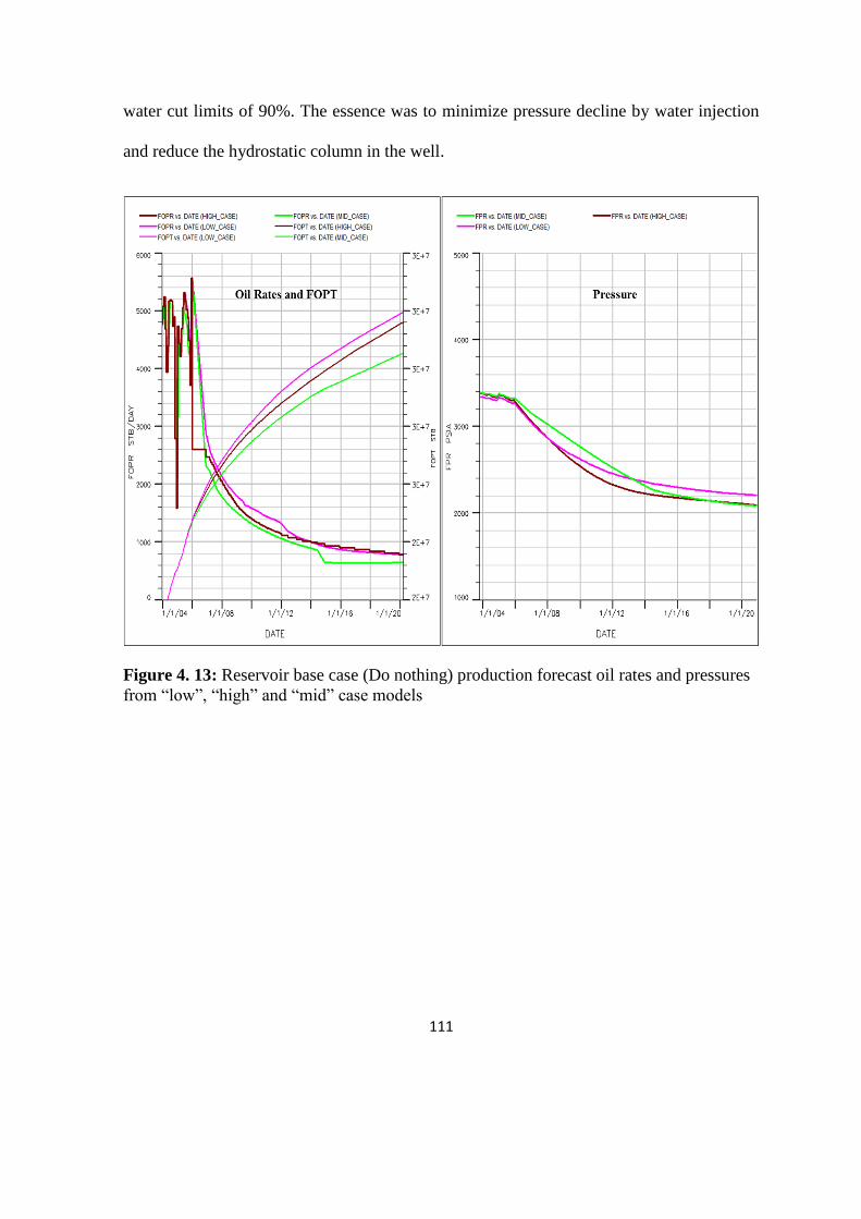
111
water cut limits of 90%. The essence was to minimize pressure decline by water injection
and reduce the hydrostatic column in the well.
Figure 4. 13: Reservoir base case (Do nothing) production forecast oil rates and pressures
from “low”, “high” and “mid” case models
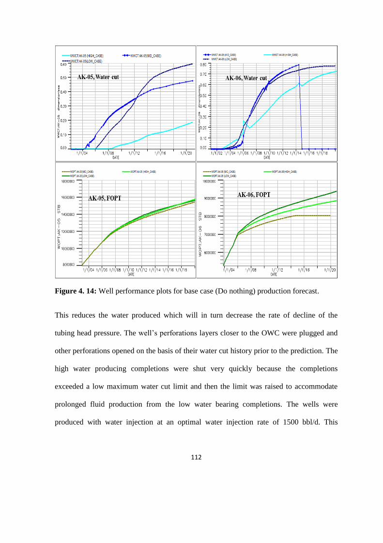
112
Figure 4. 14: Well performance plots for base case (Do nothing) production forecast.
This reduces the water produced which will in turn decrease the rate of decline of the
tubing head pressure. The well’s perforations layers closer to the OWC were plugged and
other perforations opened on the basis of their water cut history prior to the prediction. The
high water producing completions were shut very quickly because the completions
exceeded a low maximum water cut limit and then the limit was raised to accommodate
prolonged fluid production from the low water bearing completions. The wells were
produced with water injection at an optimal water injection rate of 1500 bbl/d. This

113
optimal water injection rate was derived from sensitivity runs using injection rates between
500 bbl/d and 2500 bbl/d.
The comparison of the reservoir performance plots for the case 1 and case 2 are presented
in Figure 4. 15. The plot shows the incremental production for the Case 2 when compared
with the base cases. Figure 4.16 compares the water cut and oil recovery for well AK-05
and AK-06 in the water injection case versus base case.
Figure 4. 15: Comparison of development Cases.

114
All dotted lines represent the trends for “Do nothing” rates, pressure and cumulative
production. Continuous lines represent rate, pressure and cumulative recovery for well
injection case.
Figure 4.16: AK-05 and AK-06 water cut and oil recovery for water injection case versus
base case.

115
The AK-05 in the high case model (Red color) exhibited delayed water breakthrough time
and therefore lowest water cut (30%) and highest production when compare with the base
case model (Green color). However, AK-06 of the low case (purple color) model shows
minimum water cut and highest oil production. The production plots for the 2 wells show
the existence and degrees of the uncertainty in the forecast figures.
4.6 Uncertainty Analysis
4.6.1 Experimental design
The following parameters were considered in the experimental design using the central
composite design of the response surface methodology.
i. Horizontal permeability (PERMX, PERMY)
ii. Water injection rate (Qwinj)
iii. Relative permeability to water (KRW)
iv. Oil Viscosity (OVISC)
v. Vertical permeability (PERMZ)
The analysis was performed using the “Low”, “Base” and “High” case models.
4.6.2 Analysis with replication
The extreme models (low and high cases) were treated as replicates of the base case. This
gives rise to a single response surface equation. Although only classical laboratory
experiments are characterized by random error, the random error in numerical simulation is
always assumed zero since repeating numerical simulation time without number does not

116
change the fundamental equation with which calculations are made except if the input data
is changed. The introduction of replications as used in this analysis treated the reservoir
models as uncertainty factors and believed to guarantee rigorous proxy model for
uncertainty quantification.
4.6.2.1 Full Factorial Design
Conducting 3-Level full factorial experiment with 5 factors can be time-consuming. A 2-
Level factorial of high resolution was chosen in that it gives a response surface of high
quality comparable to other response surface designs. Table 4.5Table 4.5: shows the range
of values of parameters for the experiments. The various combinations of the uncertain
parameters were generated and their responses were derived using the history matched
models in forecast mode. Thus the experiment was performed three times (with 3 models)
according to design.
Table 4.5: Uncertainty factors, their descriptions and range of values as multiplier on the
base case value
S/N
Parameters
Keywords
Multiplier Ranges
Minimum
Value
Base Case
Value
Maximum
Value
1 Oil Viscosity OVISC 0.9 1 1.1
2 Horizontal Permeability PERMX 0.57 1 1.29
3 Vertical Permeability PERMZ 0.5 1 6
4 Water relative permeability KRW 0.36 1 1.25
5 Water injection rate Qwinj 0.33 1 1.33

117
Table 4.6 shows the design matrix comprises of 96 (32 each for three models) experiments
involving the three models. The design matrix consisted of the parameter values in coded
form as well as the actual response values in stock-tank barrels after experimentation.
Figure 4. 17 shows half normal plot that shows interactively, how the factors were
selected. From Figure 4. 17, the main factors, horizontal permeability (A), vertical
permeability (B), water relative permeability (C), oil viscosity (D) and water injection rate
(E) were selected together with two factorial effect represented by the interaction of
horizontal permeability and water injection rate (AE) and interaction of vertical
permeability and water injection rate (BE).
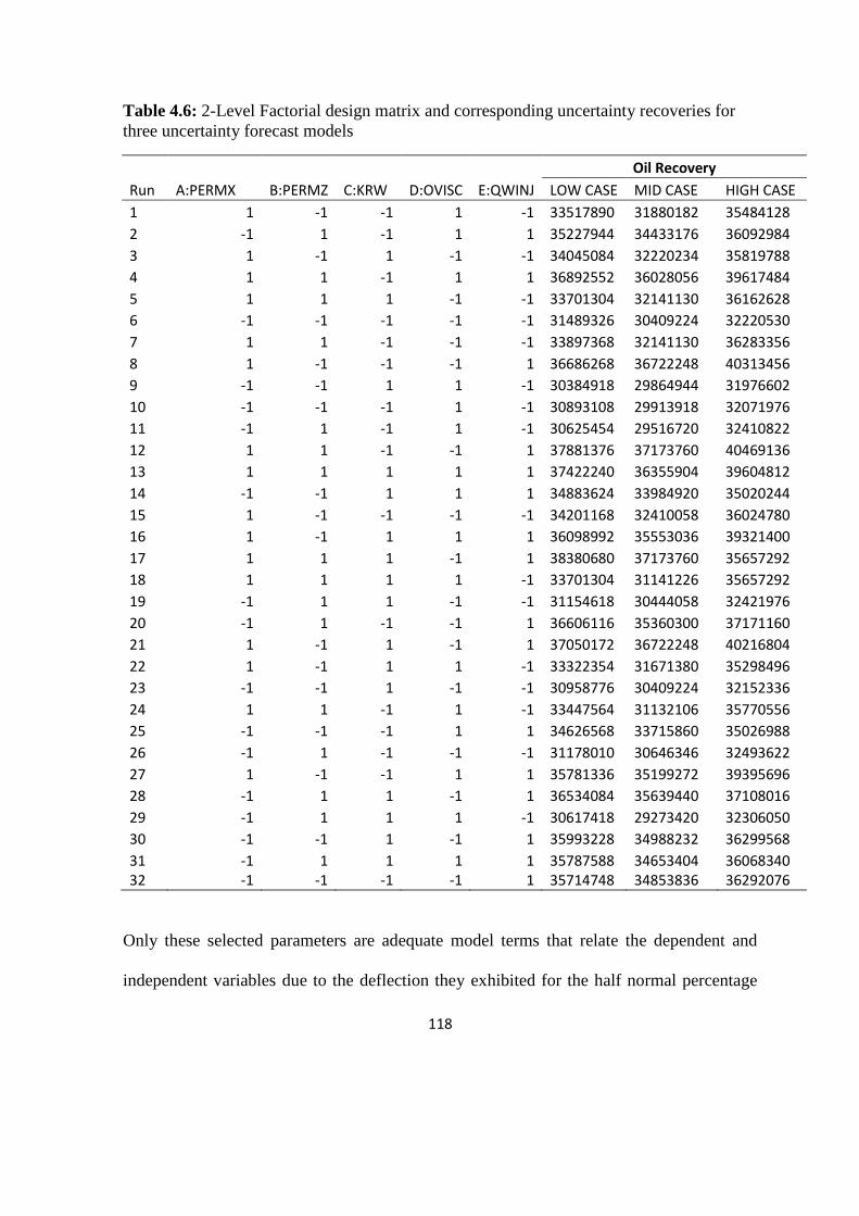
118
Table 4.6: 2-Level Factorial design matrix and corresponding uncertainty recoveries for
three uncertainty forecast models
Run A:PERMX B:PERMZ C:KRW D:OVISC E:QWINJ
Oil Recovery
LOW CASE MID CASE HIGH CASE
1 1 -1 -1 1 -1 33517890 31880182 35484128
2 -1 1 -1 1 1 35227944 34433176 36092984
3 1 -1 1 -1 -1 34045084 32220234 35819788
4 1 1 -1 1 1 36892552 36028056 39617484
5 1 1 1 -1 -1 33701304 32141130 36162628
6 -1 -1 -1 -1 -1 31489326 30409224 32220530
7 1 1 -1 -1 -1 33897368 32141130 36283356
8 1 -1 -1 -1 1 36686268 36722248 40313456
9 -1 -1 1 1 -1 30384918 29864944 31976602
10 -1 -1 -1 1 -1 30893108 29913918 32071976
11 -1 1 -1 1 -1 30625454 29516720 32410822
12 1 1 -1 -1 1 37881376 37173760 40469136
13 1 1 1 1 1 37422240 36355904 39604812
14 -1 -1 1 1 1 34883624 33984920 35020244
15 1 -1 -1 -1 -1 34201168 32410058 36024780
16 1 -1 1 1 1 36098992 35553036 39321400
17 1 1 1 -1 1 38380680 37173760 35657292
18 1 1 1 1 -1 33701304 31141226 35657292
19 -1 1 1 -1 -1 31154618 30444058 32421976
20 -1 1 -1 -1 1 36606116 35360300 37171160
21 1 -1 1 -1 1 37050172 36722248 40216804
22 1 -1 1 1 -1 33322354 31671380 35298496
23 -1 -1 1 -1 -1 30958776 30409224 32152336
24 1 1 -1 1 -1 33447564 31132106 35770556
25 -1 -1 -1 1 1 34626568 33715860 35026988
26 -1 1 -1 -1 -1 31178010 30646346 32493622
27 1 -1 -1 1 1 35781336 35199272 39395696
28 -1 1 1 -1 1 36534084 35639440 37108016
29 -1 1 1 1 -1 30617418 29273420 32306050
30 -1 -1 1 -1 1 35993228 34988232 36299568
31 -1 1 1 1 1 35787588 34653404 36068340 32 -1 -1 -1 -1 1 35714748 34853836 36292076
Only these selected parameters are adequate model terms that relate the dependent and
independent variables due to the deflection they exhibited for the half normal percentage
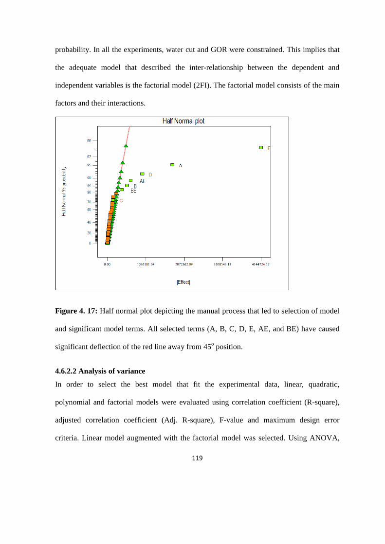
119
probability. In all the experiments, water cut and GOR were constrained. This implies that
the adequate model that described the inter-relationship between the dependent and
independent variables is the factorial model (2FI). The factorial model consists of the main
factors and their interactions.
Figure 4. 17: Half normal plot depicting the manual process that led to selection of model
and significant model terms. All selected terms (A, B, C, D, E, AE, and BE) have caused
significant deflection of the red line away from 45o position.
4.6.2.2 Analysis of variance
In order to select the best model that fit the experimental data, linear, quadratic,
polynomial and factorial models were evaluated using correlation coefficient (R-square),
adjusted correlation coefficient (Adj. R-square), F-value and maximum design error
criteria. Linear model augmented with the factorial model was selected. Using ANOVA,

120
significance of the model as well as regression parameters gave most accuracy required.
The statistical indexes used include F and p statistics. From Table 4.7, the Model F-value
of 116.05 implies the factorial model selected is significant. There is only a 0.01%
probability that a "Model F-Value" this large could occur due to noise. For the selection of
the independent variables, values of "Prob > F" less than 0.0500 indicate models terms are
significant. In this case A, B, D, E, AE and BE are the only significant model terms for
the construction of response surface. Thus factor C (KRW) is not signficant on the model
and therefore removed from the regression process of response surface development.
Table 4.7: Analysis of variance showing significance of model terms
Factor Sum of Squares DF Mean Squares F- Value Prob>F
Intercept 3.60E+14 7 5.15E+13 116.05 < 0.0001 significant
A-PERMX 5.34E+13 1 5.34E+13 120.4 < 0.0001
B-PERMZ 3.56E+12 1 3.56E+12 8.03 0.00630
C-KRW 3.39E+11 1 3.39E+11 0.76 0.38570*
D-OVISC 1.67E+13 1 1.67E+13 37.7 < 0.0001
E-QWINJ 2.34E+14 1 2.34E+14 528.26 < 0.0001
AE 6.66E+12 1 6.66E+12 15.01 0.0003
BE 2.63E+12 1 2.63E+12 5.93 0.0179
* not significant model term at 95% confidence interval
The regression equation relating ultimate recovery (dependent variable) and the history
match variables (independent variables) is equation 4.1. The responses were transformed
into logarithmic form to address non-linearity observed between the dependent and
independent variables.
Log10FOPTReplicate = 7.51467 + 0.040431 ∗ PERMX − 2.29e − 03 ∗ PERMZ + 1.83e −
03 ∗ KRW − 0.06368 ∗ OVISC + 0.05981 ∗ Qwinj − 0.01937 ∗ PERMX ∗ Qwinj +
9.58e − 03 ∗ PERMZ ∗ Qwinj 4.1
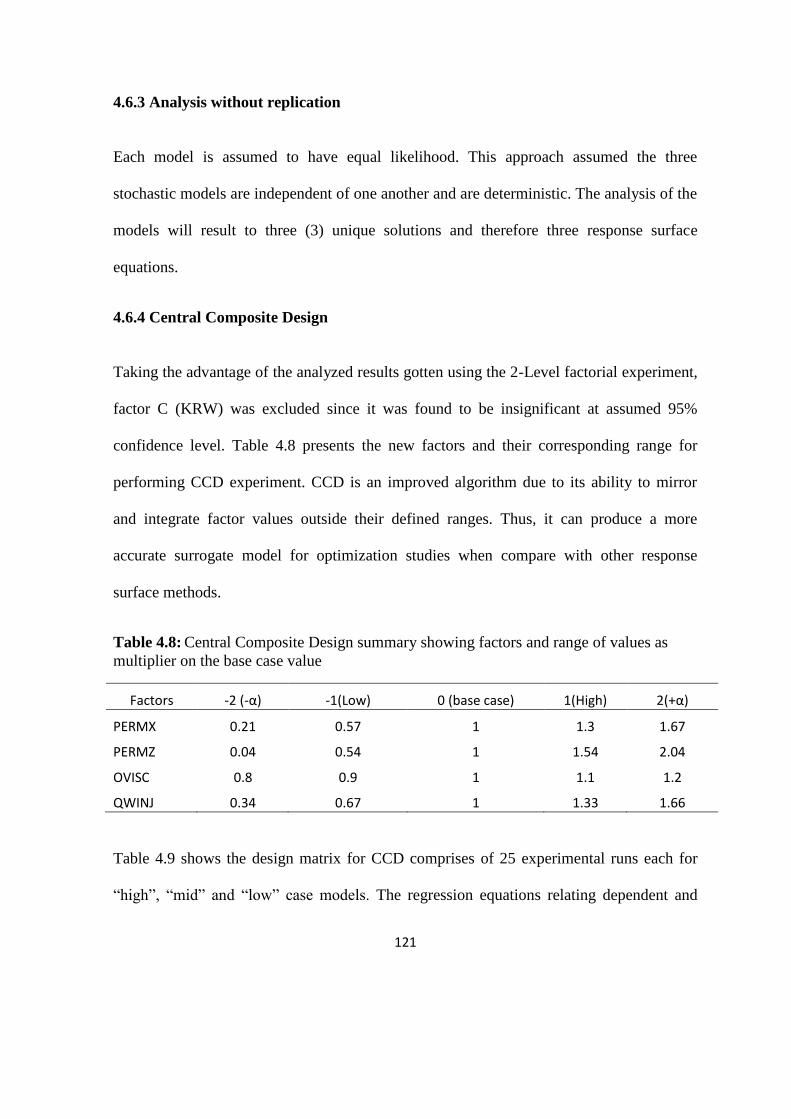
121
4.6.3 Analysis without replication
Each model is assumed to have equal likelihood. This approach assumed the three
stochastic models are independent of one another and are deterministic. The analysis of the
models will result to three (3) unique solutions and therefore three response surface
equations.
4.6.4 Central Composite Design
Taking the advantage of the analyzed results gotten using the 2-Level factorial experiment,
factor C (KRW) was excluded since it was found to be insignificant at assumed 95%
confidence level. Table 4.8 presents the new factors and their corresponding range for
performing CCD experiment. CCD is an improved algorithm due to its ability to mirror
and integrate factor values outside their defined ranges. Thus, it can produce a more
accurate surrogate model for optimization studies when compare with other response
surface methods.
Table 4.8: Central Composite Design summary showing factors and range of values as
multiplier on the base case value
Factors -2 (-α) -1(Low) 0 (base case) 1(High) 2(+α)
PERMX 0.21 0.57 1 1.3 1.67
PERMZ 0.04 0.54 1 1.54 2.04
OVISC 0.8 0.9 1 1.1 1.2
QWINJ 0.34 0.67 1 1.33 1.66
Table 4.9 shows the design matrix for CCD comprises of 25 experimental runs each for
“high”, “mid” and “low” case models. The regression equations relating dependent and

122
independent variables for low case (FOPTLow Case), Mid/Base case (FOPTBase Case) and high
case (FOPTHigh Case) are presented in equations 4.2 - 4.4. The responses were transformed
into logarithmic form to address non-linearity observed between the dependent and
independent variables.
log10FOPTLow Case = a0 + a1 ∗ PERMX + a2 ∗ PERMZ + a3 ∗ OVISC + a4 ∗ QWINJ + a5 ∗
PERMX2 + a6 ∗ OVISC2 + a7 ∗ PERMX ∗ PERMZ + a8 ∗ PERMX ∗ OVISC + a9 ∗
PERMX ∗ QWINJ + a10 ∗ PERMZ ∗ QWINJ 4.2
Log10FOPTBase Case = b0 + b1 ∗ PERMX + b2 ∗ PERMZ + b3 ∗ OVISC + b4 ∗ QWINJ +
b5 ∗ PERMX2 + b6 ∗ PERMZ2 + b7 ∗ OVISC2 + b8 ∗ PERMX ∗ PERMZ + b9 ∗ PERMX ∗
OVISC + b10 ∗ PERMX ∗ QWINJ + b11 ∗ PERMZ ∗ QWINJ 4.3
Log10FOPTHigh Case = c0 + c1 ∗ PERMX + c2 ∗ PERMZ + c3 ∗ OVISC + c4 ∗ QWINJ + c5 ∗
PERMX2 + c6 ∗ PERMZ2 + c7 ∗ OVISC2 + c8 ∗ PERMX ∗ PERMZ + c9 ∗ PERMX ∗ OVISC + c10 ∗
PERMX ∗ QWINJ + c11 ∗ PERMZ ∗ QWINJ 4.4
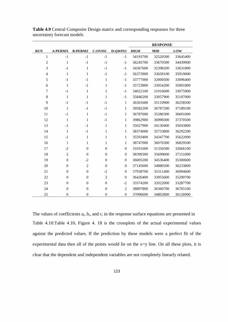
123
Table 4.9 Central Composite Design matrix and corresponding responses for three
uncertainty forecast models
RESPONSE
RUN A:PERMX B:PERMZ C:OVISC D:QWINJ HIGH MID LOW
1 -1 -1 -1 -1 34193700 32520500 33645400
2 1 -1 -1 -1 36245700 33670500 34439900
3 -1 1 -1 -1 34367600 32398200 33631800
4 1 1 -1 -1 36373900 33658100 35919000
5 -1 -1 1 -1 33777000 32000500 33096400
6 1 -1 1 -1 35723800 33054200 35001800
7 -1 1 1 -1 34022100 31916600 33075900
8 1 1 1 -1 35846200 33057900 35107000
9 -1 -1 -1 1 36301600 35110900 36258500
10 1 -1 -1 1 39582200 36787200 37189100
11 -1 1 -1 1 36787600 35280300 36601000
12 1 1 -1 1 39862900 36998300 37370500
13 -1 -1 1 1 35027900 34130400 35043800
14 1 -1 1 1 38374000 35733800 36292200
15 -1 1 1 1 35593400 34347700 35622000
16 1 1 1 1 38747000 36076300 36829500
17 -2 0 0 0 31031600 31356500 32666100
18 2 0 0 0 38399300 35699600 37151000
19 0 -2 0 0 36005200 34536400 35300600
20 0 2 0 0 37145600 34880500 36233800
21 0 0 -2 0 37938700 35311400 36994600
22 0 0 2 0 36426400 33955600 35290700
23 0 0 0 -2 33374200 32022000 33287700
24 0 0 0 2 38897800 36360700 36765100
25 0 0 0 0 37096600 34802800 36126900
The values of coefficients ai, bi, and ci in the response surface equations are presented in
Table 4.10:Table 4.10. Figure 4. 18 is the crossplots of the actual experimental values
against the predicted values. If the prediction by these models were a perfect fit of the
experimental data then all of the points would lie on the x=y line. On all these plots, it is
clear that the dependent and independent variables are not completely linearly related.
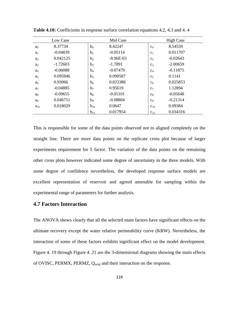
124
Table 4.10: Coefficients in response surface correlation equations 4.2, 4.3 and 4. 4
Low Case Mid Case High Case
a0 8.37734 b0 8.42247 c0 8.54559
a1 -0.04839 b1 -0.05114 c1 0.011707
a2 0.042125 b2 -8.96E-03 c2 -0.02643
a3 -1.72603 b3 -1.7891 c3 -2.00659
a4 -0.06088 b4 -0.07479 c4 -0.11875
a5 0.095946 b5 0.090587 c5 0.1141
a6 0.93066 b6 0.023388 c6 0.025853
a7 -0.04885 b7 0.95619 c7 1.12894
a8 -0.09655 b8 -0.05101 c8 -0.05648
a9 0.046751 b9 -0.08804 c9 -0.21314
a10 0.018029 b10 0.0647 c10 0.09384
b11 0.017954 c11 0.034316
This is responsible for some of the data points observed not to aligned completely on the
straight line. There are more data points on the replicate cross plot because of larger
experiments requirement for 5 factor. The variation of the data points on the remaining
other cross plots however indicated some degree of uncertainty in the three models. With
some degree of confidence nevertheless, the developed response surface models are
excellent representation of reservoir and agreed amenable for sampling within the
experimental range of parameters for further analysis.
4.7 Factors Interaction
The ANOVA shows clearly that all the selected main factors have significant effects on the
ultimate recovery except the water relative permeability curve (KRW). Nevertheless, the
interaction of some of these factors exhibits significant effect on the model development.
Figure 4. 19 through Figure 4. 21 are the 3-dimensional diagrams showing the main effects
of OVISC, PERMX, PERMZ, Qwinj and their interaction on the response.
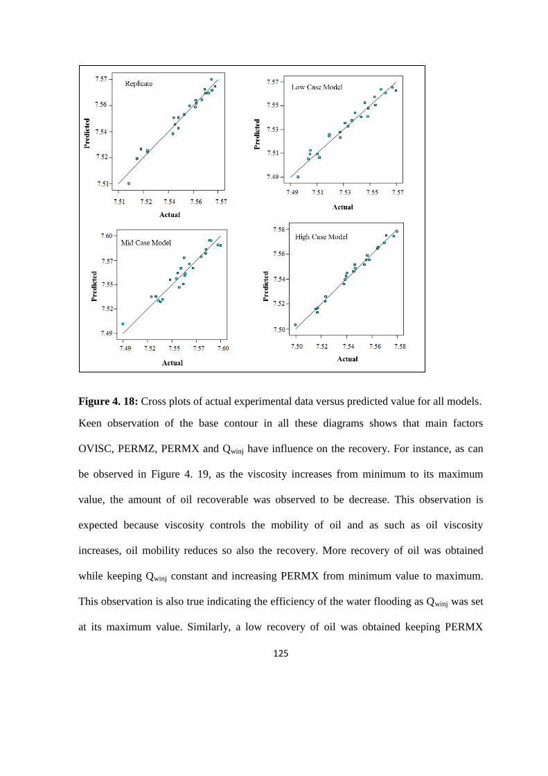
125
Figure 4. 18: Cross plots of actual experimental data versus predicted value for all models.
Keen observation of the base contour in all these diagrams shows that main factors
OVISC, PERMZ, PERMX and Qwinj have influence on the recovery. For instance, as can
be observed in Figure 4. 19, as the viscosity increases from minimum to its maximum
value, the amount of oil recoverable was observed to be decrease. This observation is
expected because viscosity controls the mobility of oil and as such as oil viscosity
increases, oil mobility reduces so also the recovery. More recovery of oil was obtained
while keeping Qwinj constant and increasing PERMX from minimum value to maximum.
This observation is also true indicating the efficiency of the water flooding as Qwinj was set
at its maximum value. Similarly, a low recovery of oil was obtained keeping PERMX

126
constant at minimum while Qwinj is at minimum. With PERMX increases to its maximum
value, a proportionate increase in recovery was observed as water injection rate increases.
This was due to preferential increase in flow of oil aerially relative to water and gas. Thus
more residual oil was contacted and swept more efficiently. Maximum recovery was
obtainable at low OVISC and moderate Qwinj. At high Qwinj, the oil recovery decreases as
the OVISC increases from minimum to maximum. This observation indicates that oil
viscosity is a huge uncertainty and the result further revealed the need to acquire more
realistic PVT data.
Figure 4. 19: 3-Dimensional diagram for the effect of water injection rate (Qwinj), oil
viscosity (OVISC) and their interaction on ultimate recovery
DESIGN-EXPERT Plot
Log10(Response 1)X = C: OVISCY = D: QWINJ
Actual FactorsA: PERMX = 0.94B: PERMZ = 1.04
7.53437
7.54398
7.5536
7.56321
7.57282
Log
(FOP
T)
0.90
0.95
1.00
1.05
1.10
0.67
0.83
1.00
1.17
1.33
C: OVISC
D: QWINJ
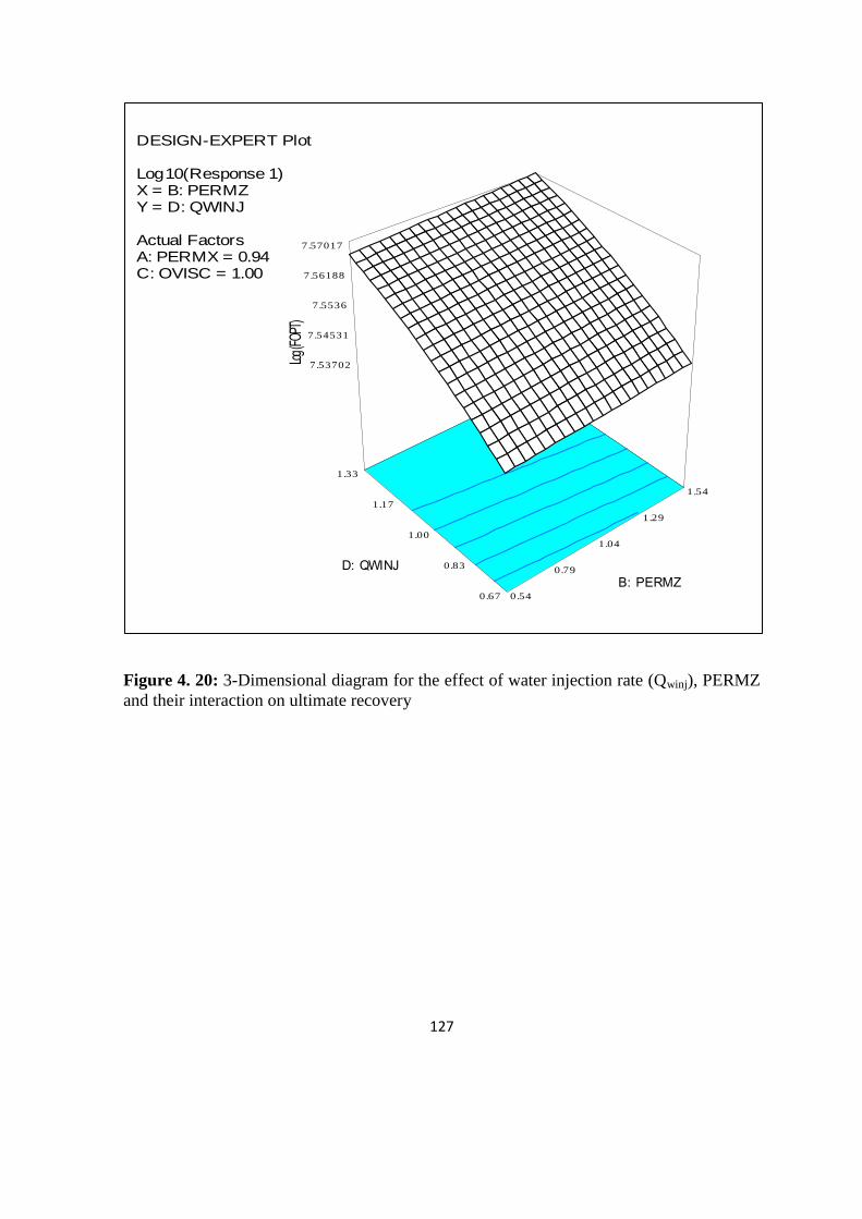
127
Figure 4. 20: 3-Dimensional diagram for the effect of water injection rate (Qwinj), PERMZ
and their interaction on ultimate recovery
DESIGN-EXPERT Plot
Log10(Response 1)X = B: PERMZY = D: QWINJ
Actual FactorsA: PERMX = 0.94C: OVISC = 1.00
7.53702
7.54531
7.5536
7.56188
7.57017
Log
(FOP
T)
0.54
0.79
1.04
1.29
1.54
0.67
0.83
1.00
1.17
1.33
B: PERMZ
D: QWINJ

128
Figure 4. 21: 3-Dimensional diagram for the effect of water injection rate (Qwinj),
PERMX and their interaction on ultimate recovery
DESIGN-EXPERT Plot
Log10(Response 1)X = A: PERMXY = D: QWINJ
Actual FactorsB: PERMZ = 1.04C: OVISC = 1.00
7.52002
7.53317
7.54632
7.55947
7.57262
Log
(FOP
T)
0.57
0.75
0.94
1.12
1.30
0.67
0.83
1.00
1.17
1.33
A: PERMX
D: QWINJ

129
4.8 Reserves Distribution
Figure 4. 22 shows the representative distributions from the Latin Hypercube sampling
comprises of 100,000 samples using different proxy models. Figure 4. 23 is a bar chart
showing P10, P50 and P90 realizations using proxy equation 4.1, 4.2, 4.3 and 4.4
compared with when the 3 models was used directly for prediction without subjected to
uncertainty analysis. The bar chart shown in Figure 4. 23 is normalized with regards to the
P50 value (34.88 Mstb). This normalization was done for easy interpretation of the result.
The P50 value is the total forecast reserves using the deterministic figure obtained from
direct forecast assuming base case/mid case model as shown in Figure 4. 24.
The Monte carlo simulation was constrained on the mean value of reserves for all the
models. In other words, the assumption of the distribution functions for different
parameters was highly dependent on the P50 realization. The mean reserves was ensured
approximated the deterministic figure of 34.88 Million barrels to provide a constraint on
the distribution function. Therefore the base case normalized value equals one (unity). The
analysis was done by considered extreme percentiles: 10-percentile (denoting a 90%
probability that the normalized reserves figures will at least greater than the 10-percentile
normalized figure) and 90 percentiles (denoting a 10% probability that the normalized
reserves figure will at most greater than the 90-percentile figures ). These figures are useful
for investment decisions. To assess the degree of uncertainty and quantify them, the
disparity between the normalized P10 and P90 figures can provide managers with
information on weither to acquire more data for detailed study or adoption of additional
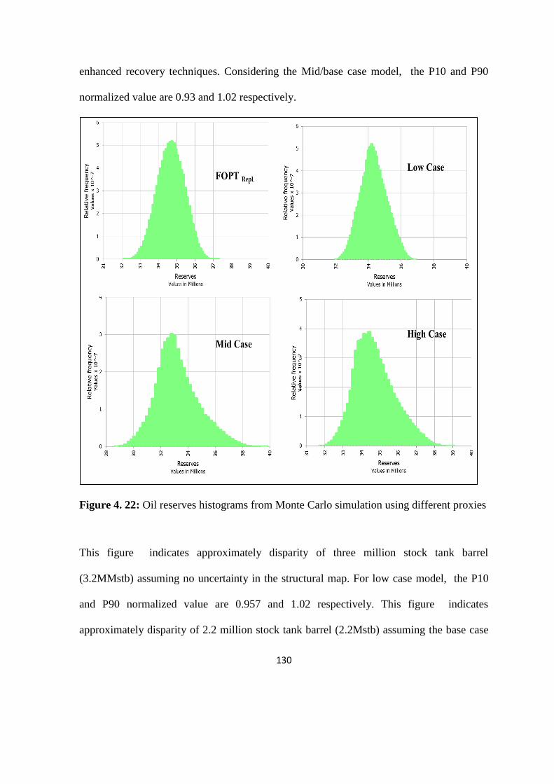
130
enhanced recovery techniques. Considering the Mid/base case model, the P10 and P90
normalized value are 0.93 and 1.02 respectively.
Figure 4. 22: Oil reserves histograms from Monte Carlo simulation using different proxies
This figure indicates approximately disparity of three million stock tank barrel
(3.2MMstb) assuming no uncertainty in the structural map. For low case model, the P10
and P90 normalized value are 0.957 and 1.02 respectively. This figure indicates
approximately disparity of 2.2 million stock tank barrel (2.2Mstb) assuming the base case

131
map was interpreted 10 ft below the base map (-10% uncertainty) . For high case model,
the P10 and P90 normalized value are 0.961 and 1.042 respectively.
Figure 4. 23: Normalized bar chart for P10, P50 and P90 realizations from simulation and
developed reservoir proxies
This figure indicates approximately disparity of 2.8 million stock tank barrel (2.8Mstb)
had it been that the base case structural map was interpreted 10ft above the base map
(+10% uncertainty). These figures represent uncertainty in the production forecast when
compare with the base case. The top and base of the sand if not properly picked can
introduce huge uncertainty. In some places, the uncertainty due to structural map can be as
high as ±50 ft this can have a huge impact on economic decisions.
0.8
0.85
0.9
0.95
1
1.05
1.1
Low Case Mid Case High Case FOPTRepl. Direct
simulation
Norm
ali
zed
per
cen
tile
Reservoir proxies
P10
P50
P90

132
Figure 4. 24: Reprisentative models analogous to P10, P50 and P90 based on simulation
approach from three history matched models
The most convention in the industry is to use the base case model then quantify uncertainty
using experimental design and Monte carlo simulation. By this approach, the P10 and P90
normalized value are 0.89 and 1.077 respectively. This figure indicates approximately
disparity of 6.5 million stock tank barrel (6.52MMstb). However, the proposed approach
(the replicates method) which we demonstrated by the integration of the three distict
uncertainty models (low, mid and high) resulted to another composite uncertainty model
upon which uncertainty analysis was based. In this method, the low and the high case
133
models are regarded as replicates of the base case which resulted in model Equation 4.1.
For FOPTRepl, the P10 and P90 normalized value are 0.91 and 1.04 respectively. This
figure indicates approximately disparity of 4.5 million stock tank barrel (4.53Mstb)
assuming ±10ft uncertaity in the structuiral map.
4.9 Summary
Structural maps was found to inherit huge uncertainty which affected the dynamic
behaviour of the reservoir. In our study we presentat an approach for quantifying
uncertainties of production forecast by incorporating uncertainty inherent in structural
maps. Three static models (a “Low”, “Mid” and “High” cases) were developed, history
matched using DoE assisted traditional method and used for production forecast. Two (2)
possible alternatives (with and without replication) were considered for uncertainty
analysis. This yielded four (4) reservoir proxies using experimental design techniques.
Uncertainty was quantified using validated proxies with Latin hypercube sampling in a
Monte Carlo simulator. There is disparity in reserves figures when compare conventional
and the new approach. Without replication, we assumed equal probability for the three
model cases and with replication we incorporated the 3 models in the design and this
offeres a more realistic answer. The result of assumption of uncertainty as small as ±10 ft
on the base case map suggested that the map has inherent uncertainty. The top and base of
the sand if not properly picked can introduce huge uncertainty and capable of impact
decision on investment and overall management of the reservoir. From the analysis carried
out, the degree of heterogeneity within the reservoir was captured by the disparity between
the P10 and P90 reserves figures. In all the cases the discripancy varied between 2.2 - 6.5

134
million stock tank barrels with the upper extreme corresponds to the conventional method
and the lower extreme the low case model. The difference suggested that the reserves
figure can vary from one company to another depending on the analysis method.
The replicate method that was introduced in this study, indicates approximately the
disparity of 4.5 million stock tank barrels. The analysis revealed with 90% certainty that at
least a normalized reserve figure of 0.91 will be realized and 10% confidence that at most
reserve figure of 1.04 will be realized. Although the conventional method overpredicted
the reserves, it can be concluded that the reservoir is fairly homogeneous due to the
proximity of these figures and injection of polymer instead of water injection will improve
the recovery because the early water breakthrough recorded in some of the wells could
actually be delayed. The method is recommendable for developing new non-complex
reservoirs/fields where subsurface data acquisition is a challenge.
135
Chapter 5
5. Infill Placement Optimization
The original problem objective of the case study 2 was to evaluate infill drilling potentials
and quantify associated uncertainty. Permeability and porosity fields are the major
uncertainties identified during the static modelling phase. Other uncertainties became
known during the history matching phase. Petrophysical properties were generated using
existing correlations. Presently, the reservoir is producing under primary recovery with
recovery factor approximate 28 %. It is desires to improve on this factor to about 35 %. It
was conceived that by reducing well spacing, well connectivity can be enhanced which in
turns improve oil recovery by accelerating production. Numerical simulation, pressure, and
saturation maps were employed to determine well locations and its optimal placement.
Evaluation and selection of infill opportunity was carried out by simulating incremental
production and water breakthrough time from vertical and horizontal wells completed
within the reservoir sub-regions.
5.1 Reservoir Descriptions of Porosity and Permeability
The top surface map and well location in this case study is shown in Figure 5. 1. There are
seven wells penetrated the reservoir. The reservoir model was constructed using a 100 x
100 x 1ft that preserve reservoir heterogeneity and accommodate simulation runs. The grid
was created using corner point geometry with dimension of 300 ft. X 300 ft. The average
porosity
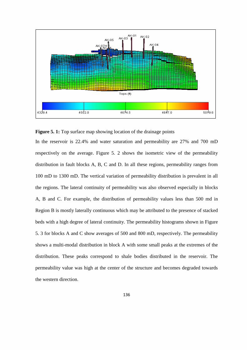
136
Figure 5. 1: Top surface map showing location of the drainage points
In the reservoir is 22.4% and water saturation and permeability are 27% and 700 mD
respectively on the average. Figure 5. 2 shows the isometric view of the permeability
distribution in fault blocks A, B, C and D. In all these regions, permeability ranges from
100 mD to 1300 mD. The vertical variation of permeability distribution is prevalent in all
the regions. The lateral continuity of permeability was also observed especially in blocks
A, B and C. For example, the distribution of permeability values less than 500 md in
Region B is mostly laterally continuous which may be attributed to the presence of stacked
beds with a high degree of lateral continuity. The permeability histograms shown in Figure
5. 3 for blocks A and C show averages of 500 and 800 mD, respectively. The permeability
shows a multi-modal distribution in block A with some small peaks at the extremes of the
distribution. These peaks correspond to shale bodies distributed in the reservoir. The
permeability value was high at the center of the structure and becomes degraded towards
the western direction.
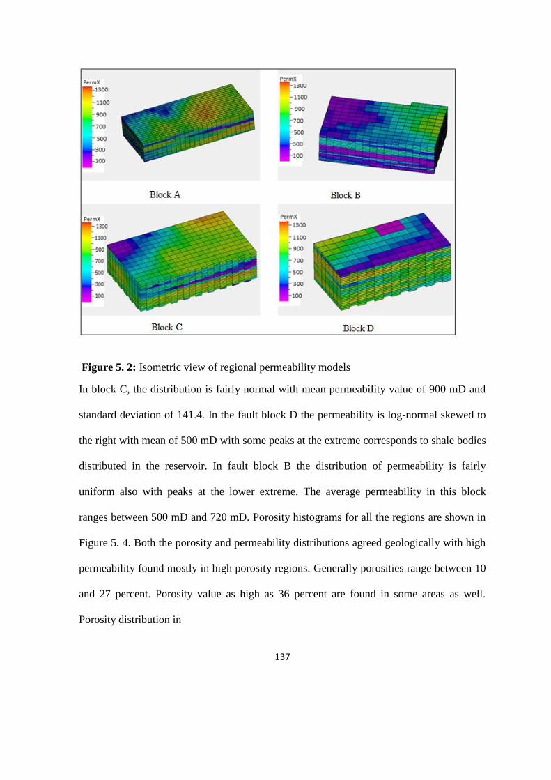
137
Figure 5. 2: Isometric view of regional permeability models
In block C, the distribution is fairly normal with mean permeability value of 900 mD and
standard deviation of 141.4. In the fault block D the permeability is log-normal skewed to
the right with mean of 500 mD with some peaks at the extreme corresponds to shale bodies
distributed in the reservoir. In fault block B the distribution of permeability is fairly
uniform also with peaks at the lower extreme. The average permeability in this block
ranges between 500 mD and 720 mD. Porosity histograms for all the regions are shown in
Figure 5. 4. Both the porosity and permeability distributions agreed geologically with high
permeability found mostly in high porosity regions. Generally porosities range between 10
and 27 percent. Porosity value as high as 36 percent are found in some areas as well.
Porosity distribution in
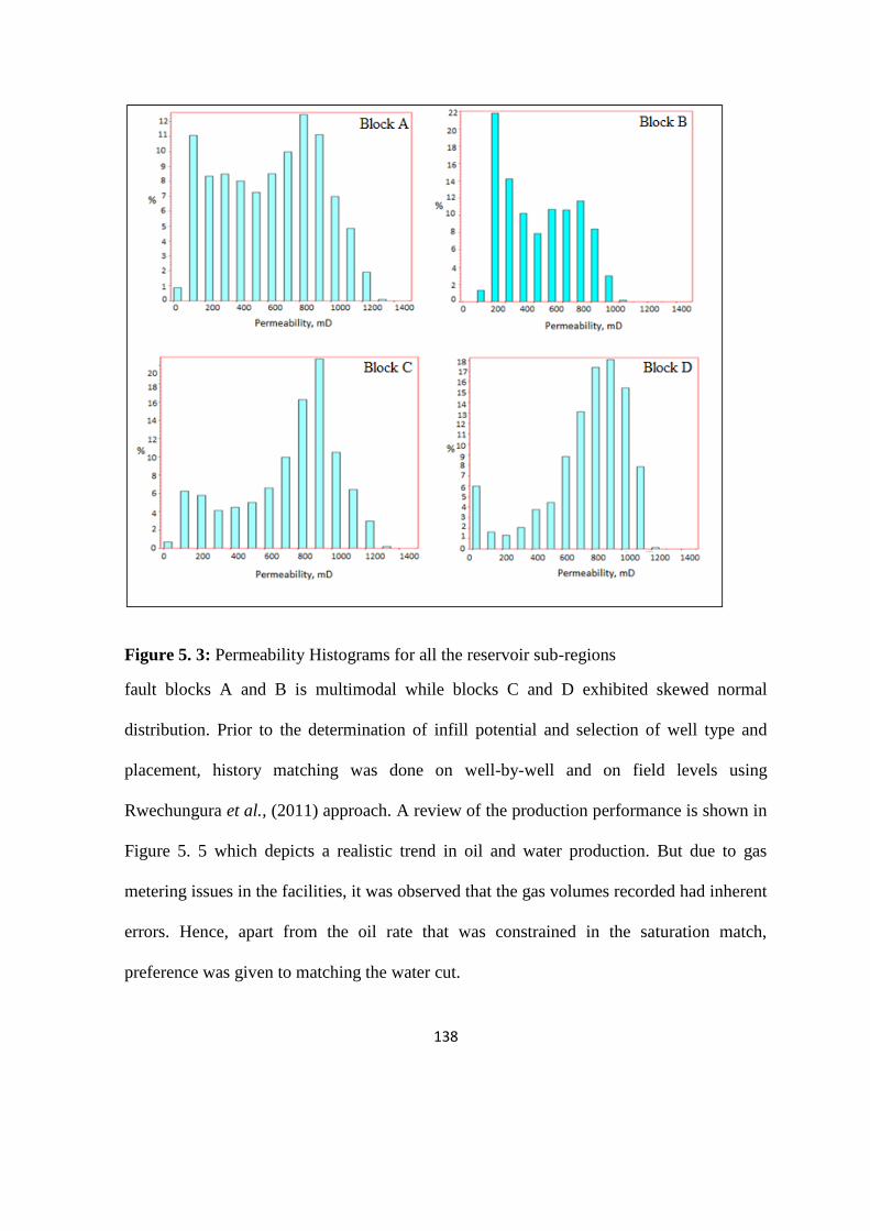
138
Figure 5. 3: Permeability Histograms for all the reservoir sub-regions
fault blocks A and B is multimodal while blocks C and D exhibited skewed normal
distribution. Prior to the determination of infill potential and selection of well type and
placement, history matching was done on well-by-well and on field levels using
Rwechungura et al., (2011) approach. A review of the production performance is shown in
Figure 5. 5 which depicts a realistic trend in oil and water production. But due to gas
metering issues in the facilities, it was observed that the gas volumes recorded had inherent
errors. Hence, apart from the oil rate that was constrained in the saturation match,
preference was given to matching the water cut.
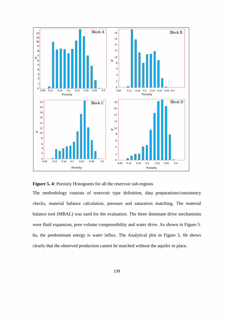
139
Figure 5. 4: Porosity Histograms for all the reservoir sub-regions
The methodology consists of reservoir type definition, data preparations/consistency
checks, material balance calculation, pressure and saturation matching. The material
balance tool (MBAL) was used for the evaluation. The three dominant drive mechanisms
were fluid expansion, pore volume compressibility and water drive. As shown in Figure 5.
6a, the predominant energy is water influx. The Analytical plot in Figure 5. 6b shows
clearly that the observed production cannot be matched without the aquifer in place.

140
Figure 5. 5: Field Production performance profiles
A steep drop in reservoir pressure when no aquifer was included indicates insufficient
energy within the reservoir. The aquifer was modelled numerically and attached to the
grid. Using appropriate aquifer pore volume, a stable pressure that fairly matched the
reservoir pressure was obtained. After a number of modifications to the aquifer size and its
permeability, the pressure match was achieved on reservoir basis.
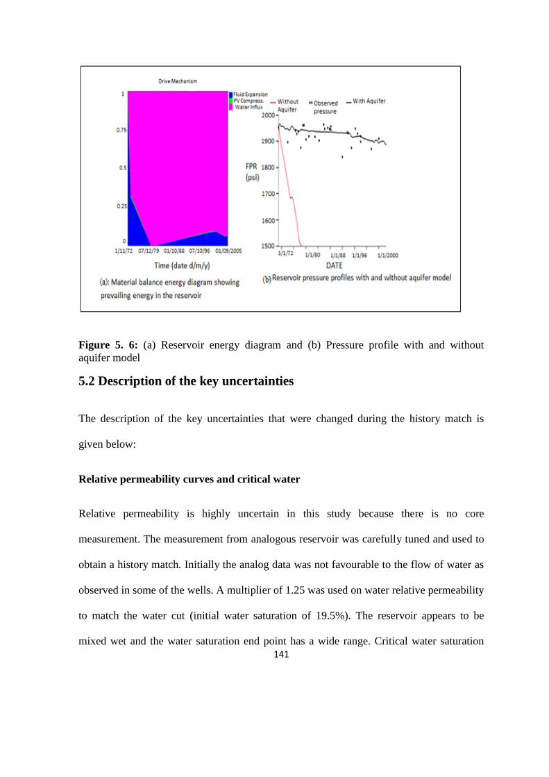
141
Figure 5. 6: (a) Reservoir energy diagram and (b) Pressure profile with and without
aquifer model
5.2 Description of the key uncertainties
The description of the key uncertainties that were changed during the history match is
given below:
Relative permeability curves and critical water
Relative permeability is highly uncertain in this study because there is no core
measurement. The measurement from analogous reservoir was carefully tuned and used to
obtain a history match. Initially the analog data was not favourable to the flow of water as
observed in some of the wells. A multiplier of 1.25 was used on water relative permeability
to match the water cut (initial water saturation of 19.5%). The reservoir appears to be
mixed wet and the water saturation end point has a wide range. Critical water saturation

142
was increased by a factor of 2 and 1.5 around well AK-06 and AK-07 to match the water
breakthrough time. The connate water saturations obtained from the static model were
relatively low.
Vertical/horizontal permeability (KV/KH)
Among the parameters that remain uncertain was the ratio of vertical to horizontal
permeability. Since the reservoir is undersaturated with no horizontal well penetrated, it
was expected that the impact of the parameter be minimal. However, the dominant of water
influx (bottom water) and proposed horizontal wells necessitates carrying this ratio further
for uncertainty analysis. PERMZ was reduced globally by a multiplying factor of 0.01.
This improved the water production in AK-01 by enhancing the lateral flow of water in
this area that allowed matching the water cut.
Fault transmissibility
A fault multiplier of 2 was applied to the fault located between AK-01 and AK-04 to match
the water influx around AK-01 well. The transmissibility of another fault towards the crest
of the reservoir was reduced by 15% as a result of the excessive gas being produced in the
model by well Ak-05.
Aquifer pore volume
Aquifer pore volume used for numerical aquifer model was sensitized upon until
satisfactory pressure and saturation match was obtained. Figure 5. 7 shows the results of
the history matching at field level. It consists of four different graphs of various responses
in the vertical axis and time on the horizontal axis. The dotted points indicate the observed

143
data while the continuous line the simulated values. The pressure match is shown in black
colour, water cut and cumulative water produced in blue and the GOR in red. Figure 5. 8
shows the water-cut match for four wells. It is clear that the breakthrough time and
observed water-cut levels were matched in all the wells. However, the mismatch observed
in field water breakthrough time was due to proximity of some wells to oil-water-contact.
Nevertheless, the field matching was considered satisfactory and suitable to use for further
evaluation.
Figure 5. 7: Field pressure and saturation match
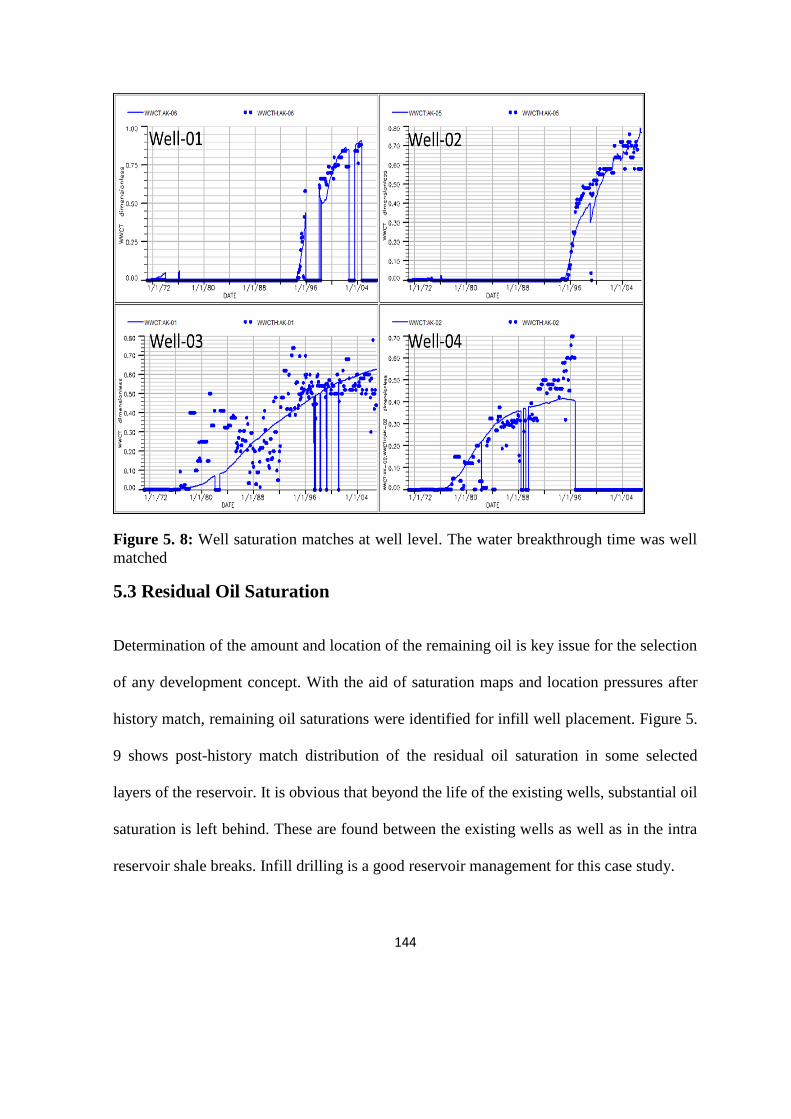
144
Figure 5. 8: Well saturation matches at well level. The water breakthrough time was well
matched
5.3 Residual Oil Saturation
Determination of the amount and location of the remaining oil is key issue for the selection
of any development concept. With the aid of saturation maps and location pressures after
history match, remaining oil saturations were identified for infill well placement. Figure 5.
9 shows post-history match distribution of the residual oil saturation in some selected
layers of the reservoir. It is obvious that beyond the life of the existing wells, substantial oil
saturation is left behind. These are found between the existing wells as well as in the intra
reservoir shale breaks. Infill drilling is a good reservoir management for this case study.
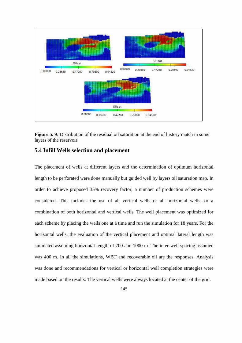
145
Figure 5. 9: Distribution of the residual oil saturation at the end of history match in some
layers of the reservoir.
5.4 Infill Wells selection and placement
The placement of wells at different layers and the determination of optimum horizontal
length to be perforated were done manually but guided well by layers oil saturation map. In
order to achieve proposed 35% recovery factor, a number of production schemes were
considered. This includes the use of all vertical wells or all horizontal wells, or a
combination of both horizontal and vertical wells. The well placement was optimized for
each scheme by placing the wells one at a time and run the simulation for 18 years. For the
horizontal wells, the evaluation of the vertical placement and optimal lateral length was
simulated assuming horizontal length of 700 and 1000 m. The inter-well spacing assumed
was 400 m. In all the simulations, WBT and recoverable oil are the responses. Analysis
was done and recommendations for vertical or horizontal well completion strategies were
made based on the results. The vertical wells were always located at the center of the grid.

146
Analog comparison method (Obor et al., 2009) was used to determine the initial
production rates because of uncertainties that characterized the available PVT data and also
due to lack of reliable well test information. Four vertical wells were strategically located
in each of the fault blocks. In each fault block, two horizontal wells were placed. The
performance of the vertical wells as well as the horizontal wells was assessed by
simulating 400, 600, 800 and 1000 stb/day. Figure 5. 10 and Figure 5. 11 compare
production rates for horizontal and vertical wells with optimal completion strategies for the
most likely reservoir characteristics. A vertical well produces at a shorter plateau period
than the horizontal well for all the simulated rates. Thus vertical wells produces at a
significantly lower plateau rate than horizontal wells placed in the same location. The
simulation was done using bottom hole pressure of 1000 and 500 psi for vertical and
horizontal wells respectively.
In all cases, the optimum rate obtained for each vertical and horizontal wells are 400 and
800 stb/day respectively.
Figure 5. 12 and Figure 5. 13 show the production performance plots for four vertical and 2
horizontal wells drilled at fault blocks B and D. It is obvious that the two horizontal well’s
performance is better compared with vertical wells. Apart from high cumulative production
of oil, horizontal wells are associated with relatively low water cut and delayed water
breakthrough time. Figure 5. 14 and Figure 5. 15 show the forecast oil and water cut for the
horizontal wells at different reservoir sub-region. The wells are located at different grid
blocks and are completed at different layers based on oil and water saturation distributions.
The profiles give a quick screening of the possible location and completion of the wells
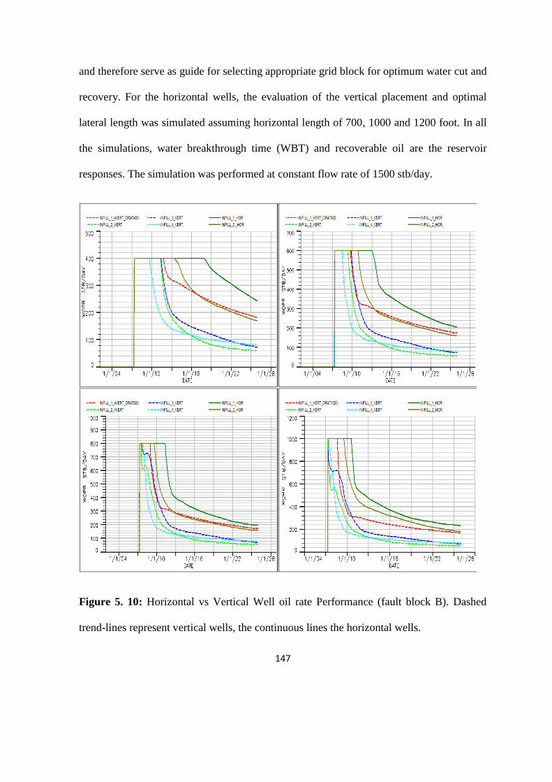
147
and therefore serve as guide for selecting appropriate grid block for optimum water cut and
recovery. For the horizontal wells, the evaluation of the vertical placement and optimal
lateral length was simulated assuming horizontal length of 700, 1000 and 1200 foot. In all
the simulations, water breakthrough time (WBT) and recoverable oil are the reservoir
responses. The simulation was performed at constant flow rate of 1500 stb/day.
Figure 5. 10: Horizontal vs Vertical Well oil rate Performance (fault block B). Dashed
trend-lines represent vertical wells, the continuous lines the horizontal wells.
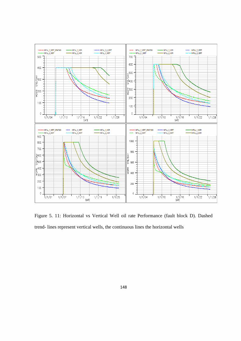
148
Figure 5. 11: Horizontal vs Vertical Well oil rate Performance (fault block D). Dashed
trend- lines represent vertical wells, the continuous lines the horizontal wells
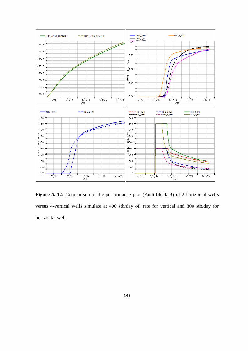
149
Figure 5. 12: Comparison of the performance plot (Fault block B) of 2-horizontal wells
versus 4-vertical wells simulate at 400 stb/day oil rate for vertical and 800 stb/day for
horizontal well.
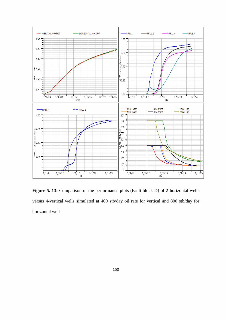
150
Figure 5. 13: Comparison of the performance plots (Fault block D) of 2-horizontal wells
versus 4-vertical wells simulated at 400 stb/day oil rate for vertical and 800 stb/day for
horizontal well
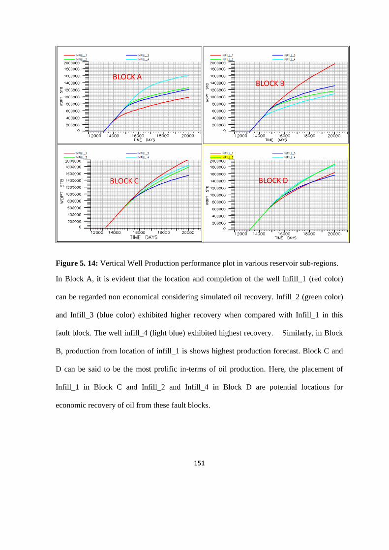
151
Figure 5. 14: Vertical Well Production performance plot in various reservoir sub-regions.
In Block A, it is evident that the location and completion of the well Infill_1 (red color)
can be regarded non economical considering simulated oil recovery. Infill_2 (green color)
and Infill_3 (blue color) exhibited higher recovery when compared with Infill_1 in this
fault block. The well infill_4 (light blue) exhibited highest recovery. Similarly, in Block
B, production from location of infill_1 is shows highest production forecast. Block C and
D can be said to be the most prolific in-terms of oil production. Here, the placement of
Infill_1 in Block C and Infill_2 and Infill_4 in Block D are potential locations for
economic recovery of oil from these fault blocks.
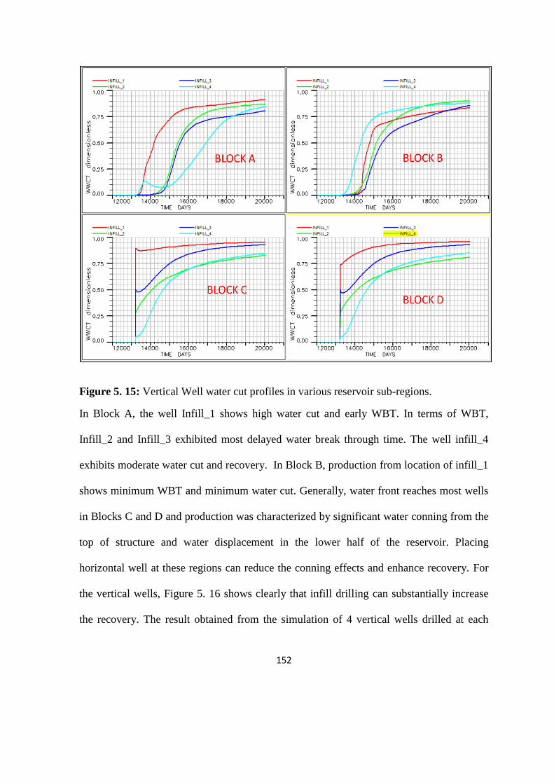
152
Figure 5. 15: Vertical Well water cut profiles in various reservoir sub-regions.
In Block A, the well Infill_1 shows high water cut and early WBT. In terms of WBT,
Infill_2 and Infill_3 exhibited most delayed water break through time. The well infill_4
exhibits moderate water cut and recovery. In Block B, production from location of infill_1
shows minimum WBT and minimum water cut. Generally, water front reaches most wells
in Blocks C and D and production was characterized by significant water conning from the
top of structure and water displacement in the lower half of the reservoir. Placing
horizontal well at these regions can reduce the conning effects and enhance recovery. For
the vertical wells, Figure 5. 16 shows clearly that infill drilling can substantially increase
the recovery. The result obtained from the simulation of 4 vertical wells drilled at each
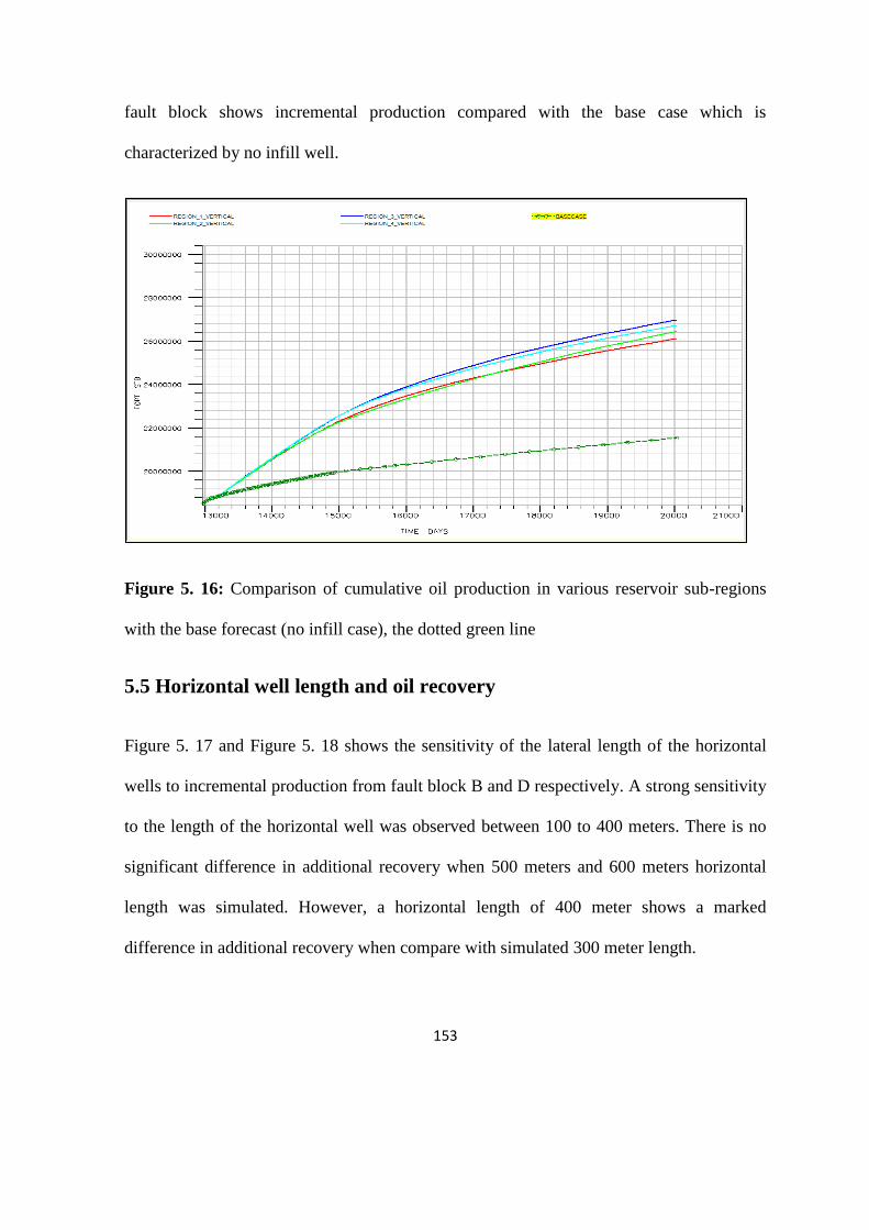
153
fault block shows incremental production compared with the base case which is
characterized by no infill well.
Figure 5. 16: Comparison of cumulative oil production in various reservoir sub-regions
with the base forecast (no infill case), the dotted green line
5.5 Horizontal well length and oil recovery
Figure 5. 17 and Figure 5. 18 shows the sensitivity of the lateral length of the horizontal
wells to incremental production from fault block B and D respectively. A strong sensitivity
to the length of the horizontal well was observed between 100 to 400 meters. There is no
significant difference in additional recovery when 500 meters and 600 meters horizontal
length was simulated. However, a horizontal length of 400 meter shows a marked
difference in additional recovery when compare with simulated 300 meter length.
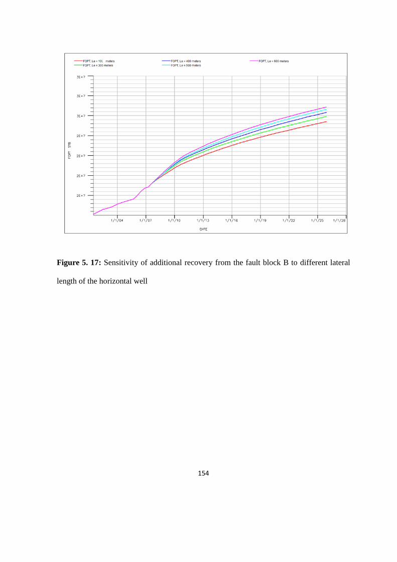
154
Figure 5. 17: Sensitivity of additional recovery from the fault block B to different lateral
length of the horizontal well
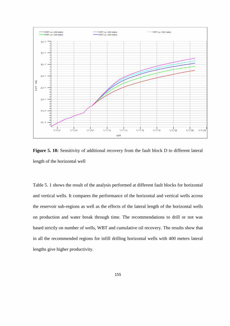
155
Figure 5. 18: Sensitivity of additional recovery from the fault block D to different lateral
length of the horizontal well
Table 5. 1 shows the result of the analysis performed at different fault blocks for horizontal
and vertical wells. It compares the performance of the horizontal and vertical wells across
the reservoir sub-regions as well as the effects of the lateral length of the horizontal wells
on production and water break through time. The recommendations to drill or not was
based strictly on number of wells, WBT and cumulative oil recovery. The results show that
in all the recommended regions for infill drilling horizontal wells with 400 meters lateral
lengths give higher productivity.
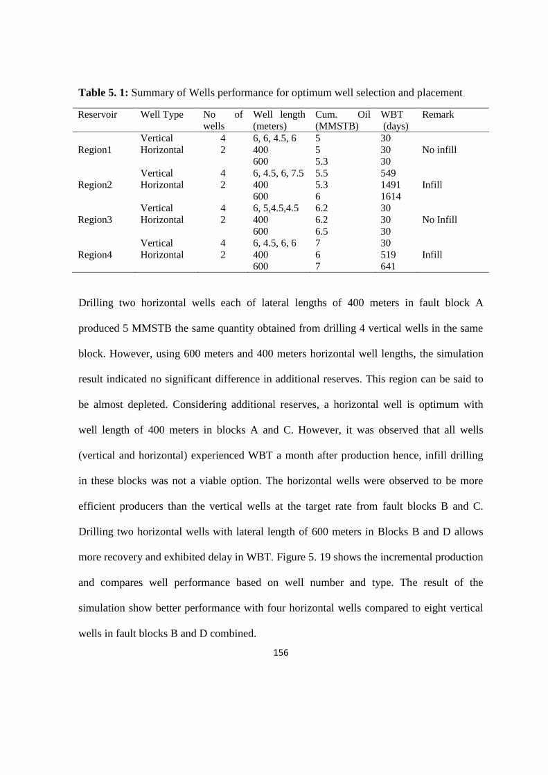
156
Table 5. 1: Summary of Wells performance for optimum well selection and placement
Reservoir Well Type No of
wells
Well length
(meters)
Cum. Oil
(MMSTB)
WBT
(days)
Remark
Vertical 4 6, 6, 4.5, 6 5 30
Region1 Horizontal 2 400 5 30 No infill
600 5.3 30
Vertical 4 6, 4.5, 6, 7.5 5.5 549
Region2 Horizontal 2 400 5.3 1491 Infill
600 6 1614
Vertical 4 6, 5,4.5,4.5 6.2 30
Region3 Horizontal 2 400 6.2 30 No Infill
600 6.5 30
Vertical 4 6, 4.5, 6, 6 7 30
Region4 Horizontal 2 400 6 519 Infill
600 7 641
Drilling two horizontal wells each of lateral lengths of 400 meters in fault block A
produced 5 MMSTB the same quantity obtained from drilling 4 vertical wells in the same
block. However, using 600 meters and 400 meters horizontal well lengths, the simulation
result indicated no significant difference in additional reserves. This region can be said to
be almost depleted. Considering additional reserves, a horizontal well is optimum with
well length of 400 meters in blocks A and C. However, it was observed that all wells
(vertical and horizontal) experienced WBT a month after production hence, infill drilling
in these blocks was not a viable option. The horizontal wells were observed to be more
efficient producers than the vertical wells at the target rate from fault blocks B and C.
Drilling two horizontal wells with lateral length of 600 meters in Blocks B and D allows
more recovery and exhibited delay in WBT. Figure 5. 19 shows the incremental production
and compares well performance based on well number and type. The result of the
simulation show better performance with four horizontal wells compared to eight vertical
wells in fault blocks B and D combined.

157
Figure 5. 19: Comparison of incremental production from vertical and horizontal wells.
The “8 vertical wells” is the total number of vertical wells drilled and completed in Blocks
B and D with 4 wells drilled each to the same regions. Likewise, total number of 4
horizontal wells was drilled with two horizontal wells drilled and completed each in
Blocks B and D respectively. For optimal number of infill well required, three horizontal
wells were drilled and simulated. First, two wells completed in Block B and one in Block
D. Then, with one horizontal well completed in Block B and two horizontal wells drilled
and completed in Block D. Block D was found to be more productive than Block B and
hence the ratio of horizontal wells simulated in Block B and D is 1:2. Based on this
analysis, two horizontal wells of 600 meters lateral length each was recommended for
drilling and evaluation in the reservoir fault blocks B and D.

158
Subsequent analysis therefore was performed using production results using the 4
recommended infill wells. Because it takes an average of 3 hours to run the simulation, a
surrogate model of the reservoir will be constructed to facilitate further analysis.
5.6 Summary
The study objective was to evaluate infill drilling potentials and quantify uncertainty
associated with infill drilling after model calibration. The active energy in the reservoir
was determined by material balance calculation. The pore volume that matched reservoir
pressure was modeled using Hurst–van Evaerdingen–Odeh radial model and implemented
using numerical model. Saturation match was achieved at reservoir level using traditional
history match approach. The major responses include field pressure and water cut. To
locate infill positions, the reservoir was divided into four sub-regions and optimization of
Infill Wells selection and placement was achieved using full-field numerical simulation
guided by saturation and pressure depletion maps.

159
Chapter 6
6. Experimental Design and Response Surface Methodology
Whenever experiments are designed, response surface models are usually developed. As
discussed in chapter 2, the essence is to approximate all experiments using a mathematical
equation that relates dependent and independent variables. The most common regression
model for approximation of computer experiments is polynomial regression. However, the
construction of such models requires consideration for the time, number of experiments
and variables. This chapter is dedicated to examining various DoE methods and provided
alternative model using adaptive neuro-fuzzy inference system.
6.1 Examination of DoE Methods
Considering all uncertainties for experimentation and analysis can be time consuming and
expensive, parameter screening are commonly done to reduce number of factors to
manageable sizes.
6.1.1 Screening DoE
Several screening algorithms are available for classical experiments during reservoir
management and evaluation. However, their adoption is often based on experimenter
descretions. So, little attentions are paid to the risks associated with decisions that
emanated from any made choices. The consequence is the underperformance of the project
when compared with the actual value. For this reason, three families of experimental
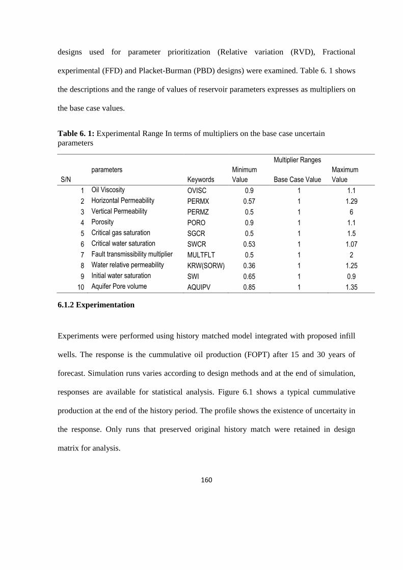
160
designs used for parameter prioritization (Relative variation (RVD), Fractional
experimental (FFD) and Placket-Burman (PBD) designs) were examined. Table 6. 1 shows
the descriptions and the range of values of reservoir parameters expresses as multipliers on
the base case values.
Table 6. 1: Experimental Range In terms of multipliers on the base case uncertain
parameters
Multiplier Ranges
S/N
parameters
Keywords
Minimum
Value Base Case Value
Maximum
Value
1 Oil Viscosity OVISC 0.9 1 1.1
2 Horizontal Permeability PERMX 0.57 1 1.29
3 Vertical Permeability PERMZ 0.5 1 6
4 Porosity PORO 0.9 1 1.1
5 Critical gas saturation SGCR 0.5 1 1.5
6 Critical water saturation SWCR 0.53 1 1.07
7 Fault transmissibility multiplier MULTFLT 0.5 1 2
8 Water relative permeability KRW(SORW) 0.36 1 1.25
9 Initial water saturation SWI 0.65 1 0.9
10 Aquifer Pore volume AQUIPV 0.85 1 1.35
6.1.2 Experimentation
Experiments were performed using history matched model integrated with proposed infill
wells. The response is the cummulative oil production (FOPT) after 15 and 30 years of
forecast. Simulation runs varies according to design methods and at the end of simulation,
responses are available for statistical analysis. Figure 6.1 shows a typical cummulative
production at the end of the history period. The profile shows the existence of uncertaity in
the response. Only runs that preserved original history match were retained in design
matrix for analysis.
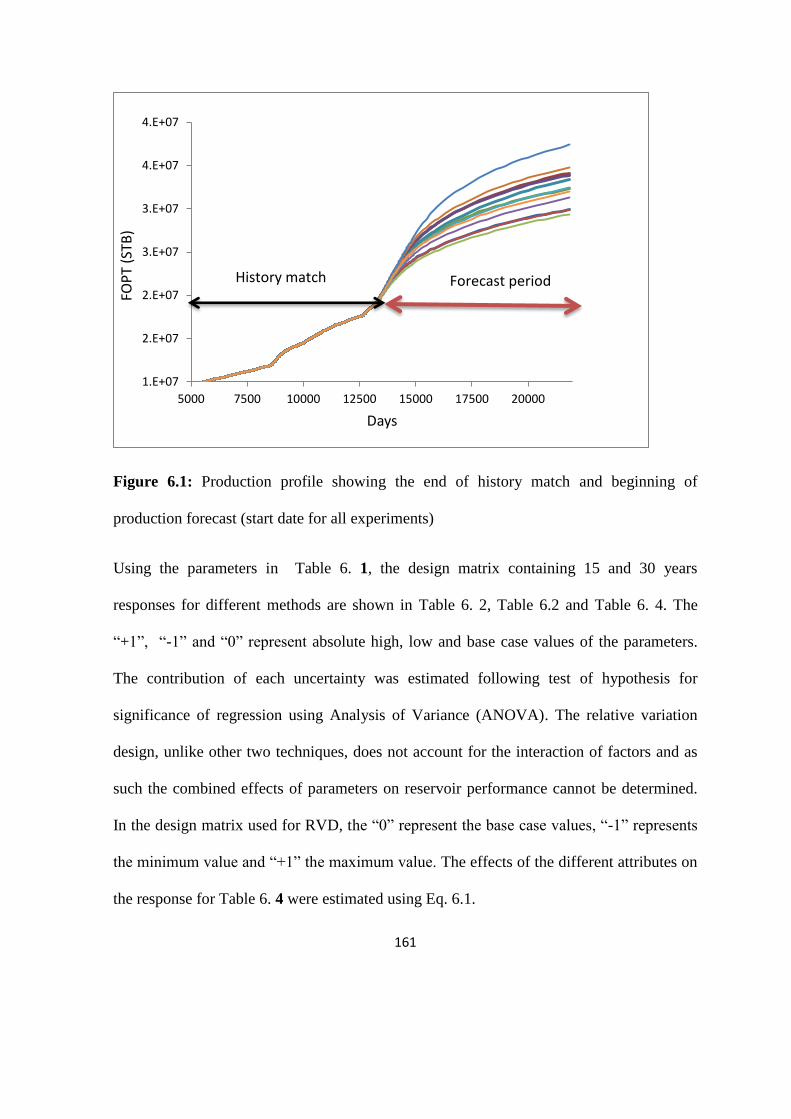
161
Figure 6.1: Production profile showing the end of history match and beginning of
production forecast (start date for all experiments)
Using the parameters in Table 6. 1, the design matrix containing 15 and 30 years
responses for different methods are shown in Table 6. 2, Table 6.2 and Table 6. 4. The
“+1”, “-1” and “0” represent absolute high, low and base case values of the parameters.
The contribution of each uncertainty was estimated following test of hypothesis for
significance of regression using Analysis of Variance (ANOVA). The relative variation
design, unlike other two techniques, does not account for the interaction of factors and as
such the combined effects of parameters on reservoir performance cannot be determined.
In the design matrix used for RVD, the “0” represent the base case values, “-1” represents
the minimum value and “+1” the maximum value. The effects of the different attributes on
the response for Table 6. 4 were estimated using Eq. 6.1.
1.E+07
2.E+07
2.E+07
3.E+07
3.E+07
4.E+07
4.E+07
5000 7500 10000 12500 15000 17500 20000
FOP
T (S
TB)
Days
History match Forecast period
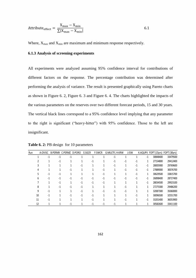
162
Attributeeffect = Xmax − Xmin
∑|Xmax − Xmin| 6.1
Where, Xmax and Xmin are maximum and minimum response respectively.
6.1.3 Analysis of screening experiments
All experiments were analyzed assuming 95% confidence interval for contributions of
different factors on the response. The percentage contribution was determined after
performing the analysis of variance. The result is presented graphically using Pareto charts
as shown in Figure 6. 2, Figure 6. 3 and Figure 6. 4. The charts highlighted the impacts of
the various parameters on the reserves over two different forecast periods, 15 and 30 years.
The vertical black lines correspond to a 95% confidence level implying that any parameter
to the right is significant (“heavy-hitter”) with 95% confidence. Those to the left are
insignificant.
Table 6. 2: PB design for 10 parameters
Run A:OVISC B:PERMX C:PERMZ D:PORO E:SGCR F:SWCR G:MULTFLTH:KRW J:ISW K:AQUPV FOPT (15yrs) FOPT (30yrs)
1 -1 -1 -1 1 1 1 -1 1 1 -1 30848400 33479500
2 1 -1 1 1 -1 1 -1 -1 -1 1 27154800 29412400
3 1 1 1 -1 1 1 -1 1 -1 -1 28005900 29769600
4 1 1 -1 1 1 -1 1 -1 -1 -1 27889000 30076700
5 -1 -1 1 1 1 -1 1 1 -1 1 30629500 33815700
6 -1 -1 -1 -1 -1 -1 -1 -1 -1 -1 26898400 28727400
7 1 -1 1 -1 -1 -1 1 1 1 -1 28034500 29923100
8 1 -1 -1 -1 1 1 1 -1 1 1 27275300 29486200
9 -1 1 1 -1 1 -1 -1 -1 1 1 32087300 35060000
10 -1 1 -1 -1 -1 1 1 1 -1 1 30096500 32551700
11 -1 1 1 1 -1 1 1 -1 1 -1 33201400 36053900
12 1 1 -1 1 -1 -1 -1 1 1 1 30582600 33411100

163
Table 6. 3: DoE matrix for fractional factorial method
Table 6. 4: Relative variation design for 10 parameters
Response, FOPT (STB)
Run A:OVISC B:PERMX C:PERMZ D:PORO E:SGCR F:SWCR G:MULTFLTH:KRW J:ISW K:AQUPV 15 Years 30 Years
1 -1 1 1 1 -1 1 -1 -1 -1 -1 29271268 33277150
2 1 -1 1 1 -1 -1 1 -1 -1 -1 25610776 28803106
3 -1 1 1 -1 -1 -1 1 1 1 -1 30558366 34219088
4 -1 -1 1 1 1 -1 -1 1 1 1 30632230 36143012
5 1 1 -1 1 -1 -1 -1 1 -1 1 27384758 31335538
6 -1 1 -1 1 1 -1 1 -1 1 -1 30327182 35035264
7 -1 1 -1 -1 1 1 -1 1 -1 -1 28117450 31376578
8 -1 -1 -1 1 -1 1 1 1 -1 1 27827028 32052148
9 1 1 1 -1 1 -1 -1 -1 -1 1 26485468 30122768
10 -1 -1 1 -1 1 1 1 -1 -1 1 27079578 31057656
11 -1 -1 -1 -1 -1 -1 -1 -1 1 1 27340390 31168096
12 1 -1 -1 -1 1 -1 1 1 -1 -1 25303208 27984070
13 1 -1 1 -1 -1 1 -1 1 1 -1 26827410 29853822
14 1 1 -1 -1 -1 1 1 -1 1 1 27344920 31090104
15 1 -1 -1 1 1 1 -1 -1 1 -1 26522916 30021116
16 1 1 1 1 1 1 1 1 1 1 30130416 35331656
Runs OVISC PERMX PERMZ PORO SGCR SWCR MULTFLTKRW SWI AQUIPV FOPT (15yrs) FOPT (30yrs)
1 1 0 0 0 0 0 0 0 0 0 29761616 35245672
2 -1 0 0 0 0 0 0 0 0 0 29116404 34489452
3 0 1 0 0 0 0 0 0 0 0 29343824 34495768
4 0 -1 0 0 0 0 0 0 0 0 29058182 34226452
5 0 0 1 0 0 0 0 0 0 0 28566772 33322416
6 0 0 -1 0 0 0 0 0 0 0 29484880 34739616
7 0 0 0 1 0 0 0 0 0 0 29502398 35138476
8 0 0 0 -1 0 0 0 0 0 0 29016448 34228136
9 0 0 0 0 1 0 0 0 0 0 28963490 34109836
10 0 0 0 0 -1 0 0 0 0 0 28046878 32737122
11 0 0 0 0 0 1 0 0 0 0 28873100 33538296
12 0 0 0 0 0 -1 0 0 0 0 28597504 33661924
13 0 0 0 0 0 0 -1 0 0 0 28902034 34034268
14 0 0 0 0 0 0 1 0 0 0 30595368 36193200
15 0 0 0 0 0 0 0 -1 0 0 27848692 32568350
16 0 0 0 0 0 0 0 1 0 0 28692348 33769084
17 0 0 0 0 0 0 0 0 -1 0 28460282 33083528
18 0 0 0 0 0 0 0 0 1 0 28978374 33975740
19 0 0 0 0 0 0 0 0 0 -1 28928676 33991664
20 0 0 0 0 0 0 0 0 0 1 26487010 30639428
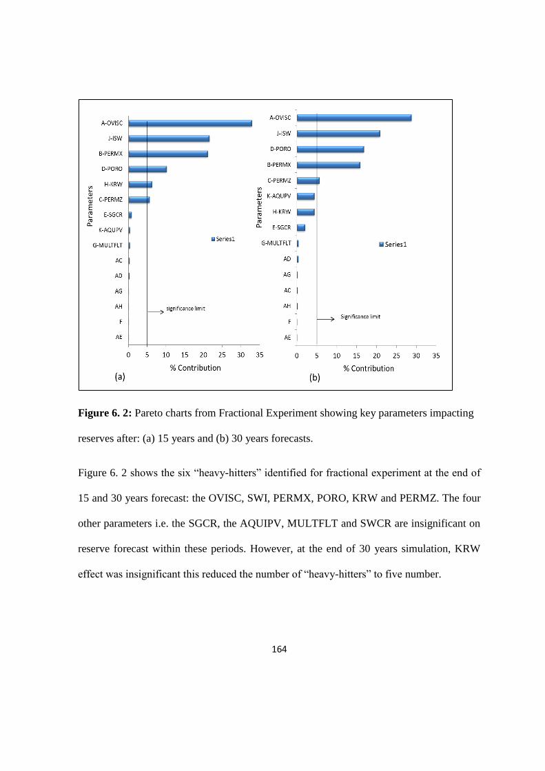
164
Figure 6. 2: Pareto charts from Fractional Experiment showing key parameters impacting
reserves after: (a) 15 years and (b) 30 years forecasts.
Figure 6. 2 shows the six “heavy-hitters” identified for fractional experiment at the end of
15 and 30 years forecast: the OVISC, SWI, PERMX, PORO, KRW and PERMZ. The four
other parameters i.e. the SGCR, the AQUIPV, MULTFLT and SWCR are insignificant on
reserve forecast within these periods. However, at the end of 30 years simulation, KRW
effect was insignificant this reduced the number of “heavy-hitters” to five number.
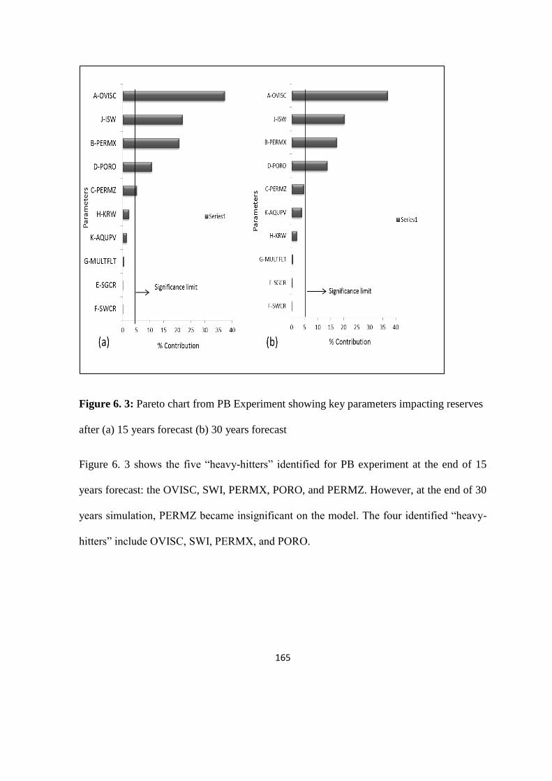
165
Figure 6. 3: Pareto chart from PB Experiment showing key parameters impacting reserves
after (a) 15 years forecast (b) 30 years forecast
Figure 6. 3 shows the five “heavy-hitters” identified for PB experiment at the end of 15
years forecast: the OVISC, SWI, PERMX, PORO, and PERMZ. However, at the end of 30
years simulation, PERMZ became insignificant on the model. The four identified “heavy-
hitters” include OVISC, SWI, PERMX, and PORO.
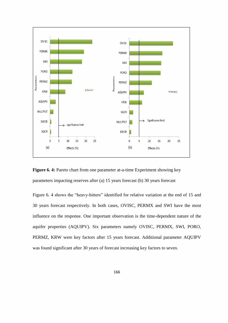
166
Figure 6. 4: Pareto chart from one parameter at-a-time Experiment showing key
parameters impacting reserves after (a) 15 years forecast (b) 30 years forecast
Figure 6. 4 shows the “heavy-hitters” identified for relative variation at the end of 15 and
30 years forecast respectively. In both cases, OVISC, PERMX and SWI have the most
influence on the response. One important observation is the time-dependent nature of the
aquifer properties (AQUIPV). Six parameters namely OVISC, PERMX, SWI, PORO,
PERMZ, KRW were key factors after 15 years forecast. Additional parameter AQUIPV
was found significant after 30 years of forecast increasing key factors to seven.

167
6.2 DoE for Response surface Model
Several 3- level designs algorithms are available for the construction of response surface
model. Similar to the screening designs, their adoption is often based on company
practices. The four families of experimental designs used for response surface modelling
considered for analysis include:
i. Box-Behnken Design (BBD)
ii. Central Composite Design (CCD)
iii. Full Factorial Design (FFD)
iv. D-Optima Design (DOD).
Table 6. 5 presents the summary of the outcome from screening analysis. The parameters
from each design are listed in order of increasing order of percentage contribution to the
response. Relative variation method identified with 7 factors. This is large compare with
the 4 and 5 factors identified with PB and FRFD respectively. The number of significant
factors dictates the number of expected experiments. The higher the number of factors the
higher the numbers of simulation runs. One important assumption that was made in this
study is the use of 2-level factorial design in place of full 3-Level factorial where the
number of key factors is greater than four. However, design resolutions were taken into
consideration. The justification for the assumption is that a 3-level full factorial design of 5
factors will require 729 experimental runs as against 32 runs by a full 2- level factorial.
Running 729 experiments is not only time consuming but also highly expensive. Instead,
making use of a 2-level full factorial is more economical depending on the objective and
stage of the project. To use 2-

168
Table 6. 5: Summary of “heavy hitters” identified using different screening methods
Relative variation Design Placket-Burman Design Fractional Factorial Design
OVISC OVISC OVISC
PERMX SWI SWI
SWI PERMX PORO
PORO PORO PERMX
PERMZ - PERMZ
KRW - -
AQUIPV - -
level factorial design for developing a response surface, proper consideration must be
given to design resolutions. Most useful resolutions for RSM are Resolution III, Resolution
IV and Resolution V. The higher the resolution the better the design but the higher is the
cost. Resolution IV designs permits freely the estimatimation of all the linear and
interaction terms so that one can conclude about the influence of each of the corresponding
parameters. Apart from this, it is economical. Table 6. 6 shows the statistical conditions for
the experiment. In general, 10 different response surfaces were developed and examined
based on the outcome from the screening methods.
Table 6. 6: Refined parameter statistics for the response surface (3-Level) experiment
Multiplier Ranges
S/N
parameters
Keywords
Minimum
Value
Base Case
Value
Maximum
Value
1 Oil Viscosity OVISC 0.9 1 1.1
2 Hor. Permeability PERMX 0.57 1 1.29
3 Vertical Permeability PERMZ 0.5 1 6
4 Porosity PORO 0.9 1 1.1
5 Relative permeability KRW(SORW) 0.36 1 1.25
6 Initial water saturation SWI 0.65 1 0.9
7 Aquifer Pore volume AQUIPV 0.85 1 1.35

169
There are 4 correlations each developed based on different factors from fractional factorial
(FRFDRSMs) and Placket-Burman (PBDRSMs) methods. Only 2 feasible response
surfaces were considered for the relative variation (RVDSMs) screening method. On all
experiments, ANOVA was performed (see Appendix B for ANOVA) for different
methods. Various design matrices are presented in the APPENDIX C. Table 6. 7 is
ANOVA result for Box-Behnken experiments associated with FRFD. The Model F-value
of 1031.25 implies the quadratic model selected is significant. There is only a 0.01%
probability that a "Model F-Value" this large could occur due to noise. The values of "Prob
> F" less than 0.0500 in Table 6. 7 indicates that all model terms are significant. In this
case PORO (A), PERMX (B), PERMZ (C), Water saturation (D), Oil viscosity (E), and
quadratic terms B2, C
2, D
2 and E
2 are significant model terms.
Table 6. 7: Analysis of variance for Box-Behnken model associated with fractional
factorial screening design
Source Sum of Squares DF Mean Square F Value Prob > F
Model 1.66E+14 9 1.85E+13 1031.25 < 0.0001 significant
A-PORO 1.58E+13 1 1.58E+13 881.42 < 0.0001
B-PERMX 1.81E+13 1 1.81E+13 1013.13 < 0.0001
C-PERMZ 7.53E+12 1 7.53E+12 420.69 < 0.0001
D-ISW 1.78E+13 1 1.78E+13 994.28 < 0.0001
E-OVISC 3.23E+13 1 3.23E+13 1806.44 < 0.0001
B2 1.87E+12 1 1.87E+12 104.26 < 0.0001
C2 1.10E+12 1 1.10E+12 61.71 < 0.0001
D2 5.66E+13 1 5.66E+13 3160.24 < 0.0001
E2 3.63E+12 1 3.63E+12 202.82 < 0.0001
Residual 6.44E+11 36 1.79E+10
Lack of Fit 6.44E+11 31 2.08E+10
Pure Error 0 5 0
Cor Total 1.67E+14 45
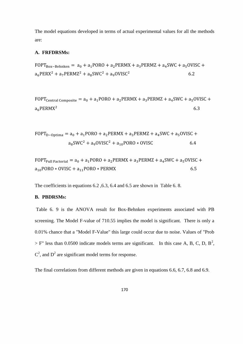
170
The model equations developed in terms of actual experimental values for all the methods
are:
A. FRFDRSMs:
FOPTBox−Behnken = a0 + a1PORO + a2PERMX + a3PERMZ + a4SWC + a5OVISC +
a6PERX2 + a7PERMZ2 + a8SWC2 + a9OVISC2 6.2
FOPTCentral Composite = a0 + a1PORO + a2PERMX + a3PERMZ + a4SWC + a5OVISC +
a6PERMX2 6.3
FOPTD−Optima = a0 + a1PORO + a2PERMX + a3PERMZ + a4SWC + a5OVISC +
a8SWC2 + a9OVISC2 + a10PORO ∗ OVISC 6.4
FOPTFull Factorial = a0 + a1PORO + a2PERMX + a3PERMZ + a4SWC + a5OVISC +
a10PORO ∗ OVISC + a11PORO ∗ PERMX 6.5
The coefficients in equations 6.2 ,6.3, 6.4 and 6.5 are shown in Table 6. 8.
B. PBDRSMs:
Table 6. 9 is the ANOVA result for Box-Behnken experiments associated with PB
screening. The Model F-value of 710.55 implies the model is significant. There is only a
0.01% chance that a "Model F-Value" this large could occur due to noise. Values of "Prob
> F" less than 0.0500 indicate models terms are significant. In this case A, B, C, D, B2,
C2, and D
2 are significant model terms for response.
The final correlations from different methods are given in equations 6.6, 6.7, 6.8 and 6.9.
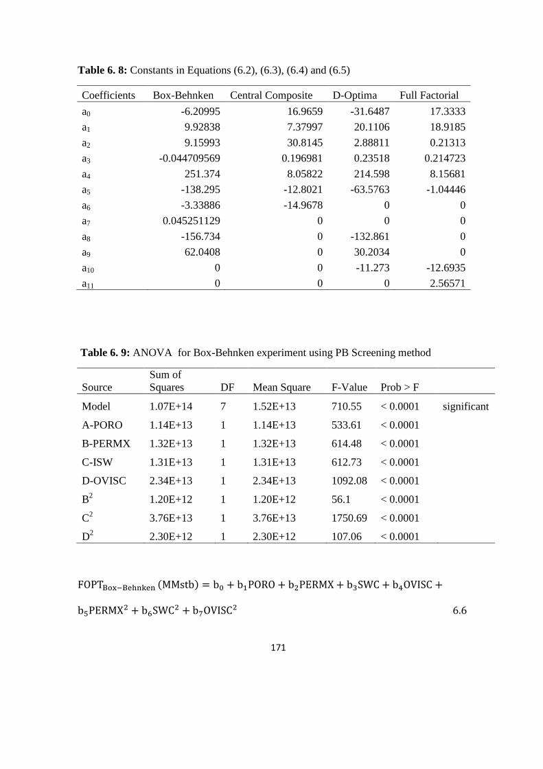
171
Table 6. 8: Constants in Equations (6.2), (6.3), (6.4) and (6.5)
Coefficients Box-Behnken Central Composite D-Optima Full Factorial
a0 -6.20995 16.9659 -31.6487 17.3333
a1 9.92838 7.37997 20.1106 18.9185
a2 9.15993 30.8145 2.88811 0.21313
a3 -0.044709569 0.196981 0.23518 0.214723
a4 251.374 8.05822 214.598 8.15681
a5 -138.295 -12.8021 -63.5763 -1.04446
a6 -3.33886 -14.9678 0 0
a7 0.045251129 0 0 0
a8 -156.734 0 -132.861 0
a9 62.0408 0 30.2034 0
a10 0 0 -11.273 -12.6935
a11 0 0 0 2.56571
Table 6. 9: ANOVA for Box-Behnken experiment using PB Screening method
Source
Sum of
Squares DF Mean Square F-Value Prob > F
Model 1.07E+14 7 1.52E+13 710.55 < 0.0001 significant
A-PORO 1.14E+13 1 1.14E+13 533.61 < 0.0001
B-PERMX 1.32E+13 1 1.32E+13 614.48 < 0.0001
C-ISW 1.31E+13 1 1.31E+13 612.73 < 0.0001
D-OVISC 2.34E+13 1 2.34E+13 1092.08 < 0.0001
B2 1.20E+12 1 1.20E+12 56.1 < 0.0001
C2 3.76E+13 1 3.76E+13 1750.69 < 0.0001
D2 2.30E+12 1 2.30E+12 107.06 < 0.0001
FOPTBox−Behnken (MMstb) = b0 + b1PORO + b2PERMX + b3SWC + b4OVISC +
b5PERMX2 + b6SWC2 + b7OVISC2 6.6

172
FOPTFFD(MMstb) = b0 + b1PORO + b2PERMX + b3SWC + b4OVISC + b5PERMX2 +
b6SWC2 + b7OVISC2 + b8PORO ∗ PERMX + b9PORO ∗ SWC + b10PORO ∗
OVISC 6.7
FOPTD−Optima(MMstb) = b0 + b1PORO + b2PERMX + b3SWC + b4OVISC +
b6SWC2 6.8
FOPTCCD(MMstb) = b0 + b1PORO + b2PERMX + b3SWC + b4OVISC + b6SWC2 6.9
The coefficients of the equations are given in Table 6. 10.
Table 6. 10: Constants in Equations (6.6), (6.7), (6.8) and (6.9)
Coefficients Box-Behnken Central Composite D-Optima Full Factorial
b0 -6.912070 -36.454900 -58.375000 -12.044100
b1 9.765720 7.873440 10.025900 13.010900
b2 8.956970 2.588430 2.904210 6.105920
b3 248.646000 179.541000 235.506000 242.231000
b4 -133.765000 -12.193800 -14.898500 -118.750000
b5 -3.254460 -111.579000 -146.385000 -3.127380
b6 -155.016000 0 0 -155.533000
b7 59.897000 0 0 58.449000
b8 0 0 0 2.572820
b9 0 0 0 7.051630
b10 0 0 0 -11.706500
C. RVDRSMs:
The seven “heavy hitters” identified with OVAAT screening include: PORO, PERMX,
PERMZ, AQUIPV, SWI, KRW and OVISC. Response surface was limited to Box-
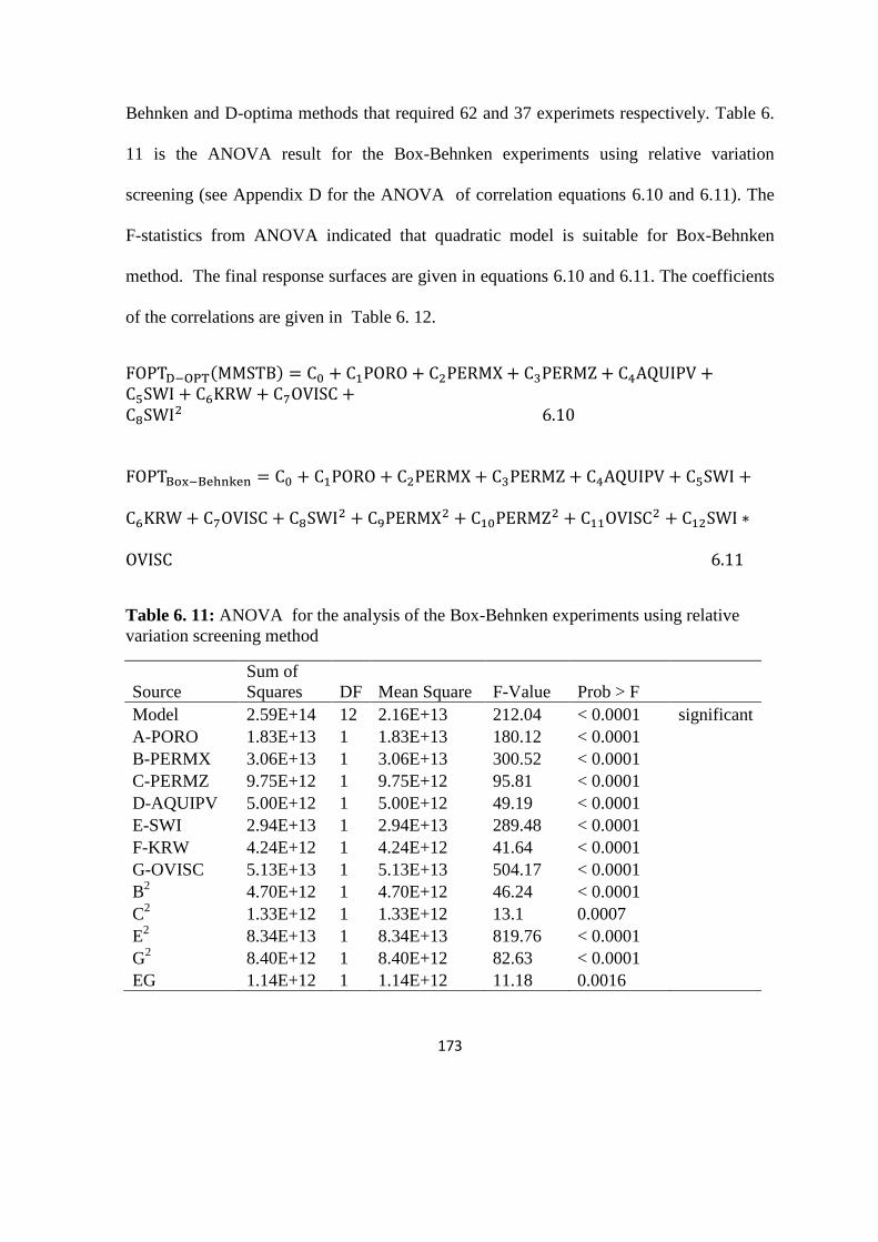
173
Behnken and D-optima methods that required 62 and 37 experimets respectively. Table 6.
11 is the ANOVA result for the Box-Behnken experiments using relative variation
screening (see Appendix D for the ANOVA of correlation equations 6.10 and 6.11). The
F-statistics from ANOVA indicated that quadratic model is suitable for Box-Behnken
method. The final response surfaces are given in equations 6.10 and 6.11. The coefficients
of the correlations are given in Table 6. 12.
FOPTD−OPT(MMSTB) = C0 + C1PORO + C2PERMX + C3PERMZ + C4AQUIPV +C5SWI + C6KRW + C7OVISC +C8SWI2 6.10
FOPTBox−Behnken = C0 + C1PORO + C2PERMX + C3PERMZ + C4AQUIPV + C5SWI +
C6KRW + C7OVISC + C8SWI2 + C9PERMX2 + C10PERMZ2 + C11OVISC2 + C12SWI ∗
OVISC 6.11
Table 6. 11: ANOVA for the analysis of the Box-Behnken experiments using relative
variation screening method
Source
Sum of
Squares DF Mean Square F-Value Prob > F
Model 2.59E+14 12 2.16E+13 212.04 < 0.0001 significant
A-PORO 1.83E+13 1 1.83E+13 180.12 < 0.0001
B-PERMX 3.06E+13 1 3.06E+13 300.52 < 0.0001
C-PERMZ 9.75E+12 1 9.75E+12 95.81 < 0.0001
D-AQUIPV 5.00E+12 1 5.00E+12 49.19 < 0.0001
E-SWI 2.94E+13 1 2.94E+13 289.48 < 0.0001
F-KRW 4.24E+12 1 4.24E+12 41.64 < 0.0001
G-OVISC 5.13E+13 1 5.13E+13 504.17 < 0.0001
B2 4.70E+12 1 4.70E+12 46.24 < 0.0001
C2 1.33E+12 1 1.33E+12 13.1 0.0007
E2 8.34E+13 1 8.34E+13 819.76 < 0.0001
G2 8.40E+12 1 8.40E+12 82.63 < 0.0001
EG 1.14E+12 1 1.14E+12 11.18 0.0016

174
Table 6. 12: Constants in Equations (6.10) and (6.11)
Coefficients Box-Behnken Method D-Optima Method
C0 34 34.29
C1 0.8737 0.8997
C2 1.129 0.9811
C3 0.6538 0.5659
C4 0.4684 0.5926
C5 1.108 1.153
C6 0.4201 0.3715
C7 -1.5 -1.431
C8 -0.5758 -2.345
C9 0.3101 0
C10 -2.424 0
C11 0.7786 0
C12 -0.3769 0
6.3 Model Validation
The data used for the development of the proxy models are presented in the Appendix C4
through C12. The response surface developed would be used during the uncertainty
quantification. The following criteria were used to assess their validity.
6.3.1 Correlation coefficients
The model validity was partly established using correlation coefficients: R-square,
Adjusted R-Square and predicted R-square values. In all equations, the R-square and
adjusted R-square values are greater than 90% which shows that the models explain at least
90% of the variability observed on the response at the points of the design. Figure 6. 5 (a, b
and c) is the parity plots for the various prediction methods, each of the four methods that
corresponds to different screening method is shown on a separate plot. These graphs are
plots of the predicted production forecast against the experimental reserves values. If the

175
prediction method were a perfect fit of the experimental data then all of the points would
lie on the x = y
Figure 6. 5: Comparison of the actual and predicted reserves by (a) FRFRSMs, (b)
PBRSMs and (c) RVDRSMs
line. By and large, the parity plots do not reveal much needed information. However, the
plots for the Box-Behnken method generally demonstrate that the method predict the actual
value more accurately. On these plots the vast majority of the points are along the x = y
line. In addition, the plots reveal that regardless of the screening method used, CCD
exhibits the least accurate prediction as this analysis revealed.

176
6.3.2 Statistical error analysis
The performance indices used for error analysis are summarized in Table 6. 13. Root
Mean square Error (RMSE) is a measure of the residuals of the model and the
experimental data. A good model is characterized by low RMSE value. Average absolute
percentage Relative Error (AAPRE) indicates the relative absolute deviation in percent
from the experimental values. A lower value implies a better correlation. In the case of a
perfect match AAPRE is zero. After the absolute percent relative error for each data point
was calculated, both the minimum (Emin) and maximum (Emax) values were scanned to
know the range of error for each model equation. The accuracy of a correlation was
examined by maximum absolute percent relative error. The lower the value of maximum
absolute percent relative error, the higher is the accuracy of the correlation.
Standard deviation (SD) is a measure of dispersion. A lower value of standard deviation
means a smaller degree of scatter. A small AD and a relatively large AAD indicates that
the errors tend to cancel (some are positive and some negative) and indicates less bias in
the prediction. If both the AD and AAD are large this indicates a bias in the prediction – a
tendency to either over predict (if the AD is negative) or under predict (if the AD is
positive) the experimental data. Each of the response surface developed was used to
estimate the production forecast for each of the data sets.Table 6.14, Table 6.15 and Table
6.16 show the result from the error analysis. In addition to the estimated errors, the
coefficients of correlations are also indicated. Box-Behnken method exhibited the least
estimation error with highest values of correlation coefficients. CCD on the other hand
shows maximum estimated error and least correlation coefficients.
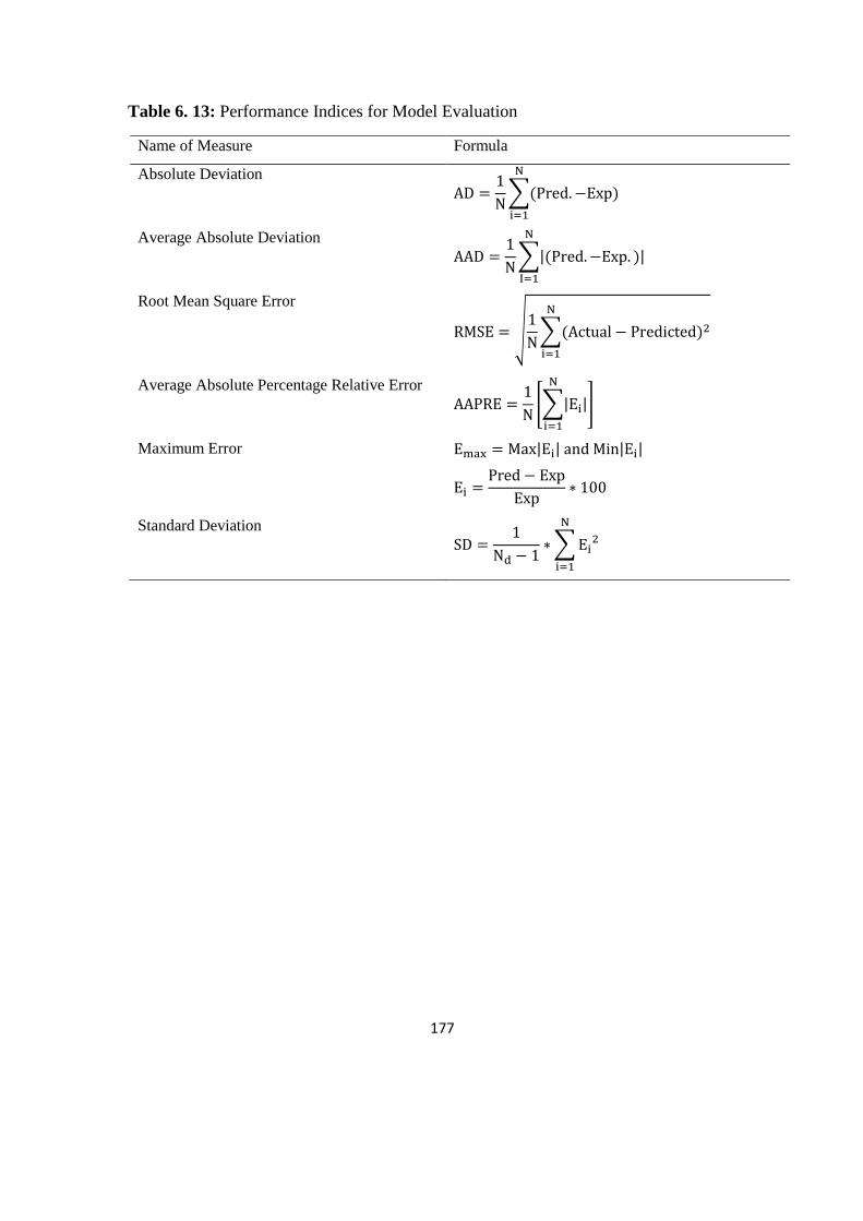
177
Table 6. 13: Performance Indices for Model Evaluation
Name of Measure Formula
Absolute Deviation
AD =1
N∑(Pred.−Exp)
N
i=1
Average Absolute Deviation
AAD =1
N∑|(Pred.−Exp. )|
N
I=1
Root Mean Square Error
RMSE = √1
N∑(Actual − Predicted)2
N
i=1
Average Absolute Percentage Relative Error
AAPRE =1
N[∑|Ei|
N
i=1
]
Maximum Error Emax = Max|Ei| and Min|Ei|
Ei =
Pred − Exp
Exp∗ 100
Standard Deviation
SD =1
Nd − 1∗ ∑Ei
2
N
i=1
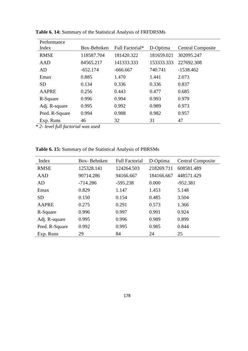
178
Table 6. 14: Summary of the Statistical Analysis of FRFDRSMs
Performance
Index Box-Behnken Full Factorial* D-Optima Central Composite
RMSE 118587.704 181420.322 181659.021 302095.247
AAD 84565.217 141333.333 153333.333 227692.308
AD -652.174 -666.667 740.741 -1538.462
Emax 0.885 1.470 1.441 2.073
SD 0.134 0.336 0.336 0.837
AAPRE 0.256 0.443 0.477 0.685
R-Square 0.996 0.994 0.993 0.979
Adj. R-square 0.995 0.992 0.989 0.973
Pred. R-Square 0.994 0.988 0.982 0.957
Exp. Runs 46 32 31 47
* 2- level full factorial was used
Table 6. 15: Summary of the Statistical Analysis of PBRSMs
Index Box- Behnken Full Factorial D-Optima Central Composite
RMSE 125328.141 124264.503 218269.711 608581.489
AAD 90714.286 94166.667 184166.667 448571.429
AD -714.286 -595.238 0.000 -952.381
Emax 0.829 1.147 1.453 5.148
SD 0.150 0.154 0.485 3.504
AAPRE 0.275 0.291 0.573 1.366
R-Square 0.996 0.997 0.991 0.924
Adj. R-square 0.995 0.996 0.989 0.899
Pred. R-Square 0.992 0.995 0.985 0.844
Exp. Runs 29 84 24 25
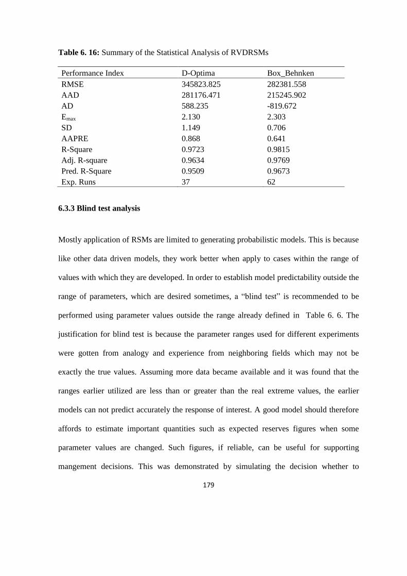
179
Table 6. 16: Summary of the Statistical Analysis of RVDRSMs
Performance Index D-Optima Box_Behnken
RMSE 345823.825 282381.558
AAD 281176.471 215245.902
AD 588.235 -819.672
Emax 2.130 2.303
SD 1.149 0.706
AAPRE 0.868 0.641
R-Square 0.9723 0.9815
Adj. R-square 0.9634 0.9769
Pred. R-Square 0.9509 0.9673
Exp. Runs 37 62
6.3.3 Blind test analysis
Mostly application of RSMs are limited to generating probabilistic models. This is because
like other data driven models, they work better when apply to cases within the range of
values with which they are developed. In order to establish model predictability outside the
range of parameters, which are desired sometimes, a “blind test” is recommended to be
performed using parameter values outside the range already defined in Table 6. 6. The
justification for blind test is because the parameter ranges used for different experiments
were gotten from analogy and experience from neighboring fields which may not be
exactly the true values. Assuming more data became available and it was found that the
ranges earlier utilized are less than or greater than the real extreme values, the earlier
models can not predict accurately the response of interest. A good model should therefore
affords to estimate important quantities such as expected reserves figures when some
parameter values are changed. Such figures, if reliable, can be useful for supporting
mangement decisions. This was demonstrated by simulating the decision whether to

180
embark on Enhance Recovery (thermal or Insitu-combustion) or stimulation using RSMs.
The study selected OVISC because it is controllable insitu by combustion, steam flooding
or injection of diluents.
Figure 6. 6 (a), (b) and (c) show respectively the comparison of RSMs with the actual
experimental values. The simulated production upon degradation of OVISC by 30, 50 and
70% is shown in Figure 6. 6 (d). It was noticed that prediction using Full Factorial method
was excellent with maximum deviation of 0.79 followed by Central Composite method
with maximum deviation of 0.9 in reserves estimation. Box-behnken generally
overpredicted the actual reserves volume with deviation approximately factor of 20.
6.3.4 Selection of response surface for analysis
Table 6. 17 summarizes various criteria used for the evaluation of all response surfaces
developed. The idea is to rank them using these measures and select the best for
uncertainty quantification. The decision to select appropriate model was based on two
scenerios:

181
Figure 6. 6: Comparison of the predictions using (a) FRFRSMs, (b) PBRSMs and (c)
RVDRSMs with the simulated reserves upon reduction of OVISC by 30, 50 and 70%.
Scenario 1:
If it is desired to develop risk curves from where only P90-P50-P10 response values and
associated parameter values are to be determined. The analysis favours the selection of
Box-Behnken method. There are however three possible response surfaces associated with
Box-behnken depending on the screening methods. These are response surface equations
6.11 (with 5 factors, 46 runs), 6.15 (with 4 factors, 29 runs) and 6.20 (with 7 factors, 62
runs). For practical purposes, response surface equation 6.15 is desirable with fewer
number of factors and experimental runs.

182
Scenario 2:
If it is desired to utilized the proxy equation for simulation and evaluation of future
development strategies such as determination of needs for acquiring additional
information, undertaking stimulation or any of EOR methods such as in-situ combustion, a
more efficient model capable of extrapolating reservoir performance within an acceptable
margin of error is desired.
Table 6. 17: Summary for model ranking
Response Surface Methods
Ranking Measures Box-Behnken
Central
Composite D-Optima
Full
factorial
Fractional Factorial
Screening Infeasible
Placket-Burman Screening
RVD Screening Infeasible Infeasible
Error Analysis Best Average Average Better
Blind test Fail Fail
Correlation R-squares
= Pass , Infeasble = not practicable due to large number of experimental runs
Both Central Composite (CCD) and Full Factorial methods are adequate. However, full
factorial method performed far better than the CCD. FFD tends to be impractical for large
number of uncertainty. We have demonstrated in this study that a 2-level factorial
experiments can be used for constructing response surface of quality comparable to that
from 3-level full factorial. However, we highly recommended consideration for the
stability and resolution of the factorial fractions to be used.
For the purpose of comparison, it was decided to select three response surface models for
uncertainty quantification. These include those associated with the Placket-Burman and
fractional factorial screening methods. They are: (a) Box-Behnken equations 6.6 (b)
Central Composite equations 6.3 (c) Full Factorial equations 6.5.

183
6.4 Uniform Experimental Design
Unlike classical experimental designs, modern experimental designs are characterized by
wider coverage of uncertainty domain and require fewer number of simulation runs.
Approximation models are usually constructed using polynomial surrogate, quadratic
model and kriging. With 4 factors the minimum number of experiments to construct a
polynomial model is given as:
P =(m + 1)(m + 2)
2⁄ 6.12
This will require at least a total of 15 experiments. Conducting 16 experiments is common
and the total of all possible combinations is 164
= 65,536. Orthogonal test designs can
reduce test number to 162 = 256; uniform design however, can reduce it to only 16 tests.
This is an advantage of modern experimental design over the conventional designs like
central composite, Box-Behnken and full factorial designs. Uniform design (UD) was used
to determine the locations of sample points within the design space. The design was
constructed such that each of the variables is divided into 16 equal levels each comprises
of only one sample point. To prevent a design that has poor space filling qualities,
Translational Propagation Algorithm (Cioppa and Lucas, 2007) was modified and
implemented in MATLAB.
Figure 6. 7 shows the schematics of initial 16 sample points (black spots) selected by UD
for a two-dimensional problem and augmented samples (red spots) that were used to
validate the model.

184
6.4.1 Quadratic model
The use of polynomial approximation model in surrogate modeling is common. Here, the
sampled data is fitted by a least-square regression technique. The accuracy of this method
depends on the highest degree of the polynomials used. However, the degree has opposite
effect on the smoothness of the representative function. To maintain balance between
interpolation accuracy, smoothness and computational expense, the “quadratic” polynomial
model was selected.
Figure 6. 7: Schematics of initial 16 sample points selected by UD for a two dimensional
design problem.
The true quadratic RSM can be written in the following form:
y(X) = y(X) + ε, X ∈ Rm 6.13
0.9
0.95
1
1.05
1.1
1.15
1.2
1.25
1.3
0 2 4 6 8 10 12 14 16 18
Var
iab
le X
1
Location
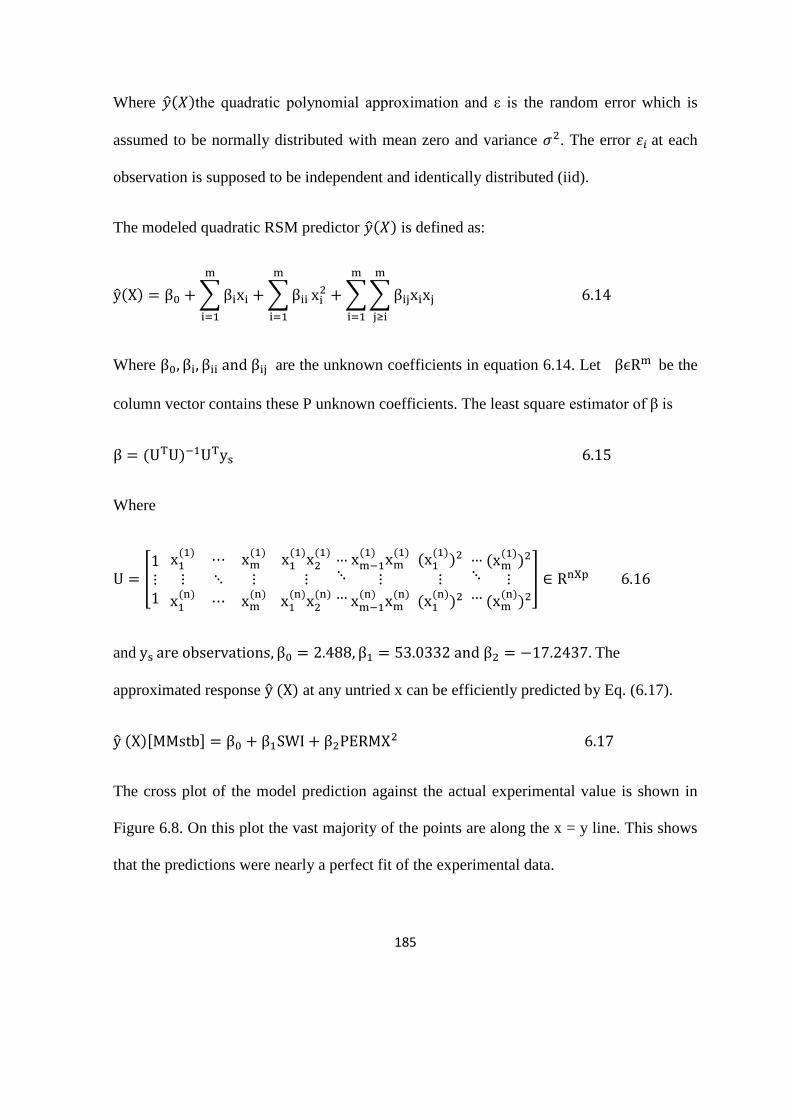
185
Where (𝑋)the quadratic polynomial approximation and ε is the random error which is
assumed to be normally distributed with mean zero and variance 𝜎2. The error 𝜀𝑖 at each
observation is supposed to be independent and identically distributed (iid).
The modeled quadratic RSM predictor (𝑋) is defined as:
y(X) = β0 + ∑βixi
m
i=1
+ ∑βii
m
i=1
xi2 + ∑∑βijxixj
m
j≥i
m
i=1
6.14
Where β0, βi, βii and βij are the unknown coefficients in equation 6.14. Let βϵRm be the
column vector contains these P unknown coefficients. The least square estimator of β is
β = (UTU)−1UTys 6.15
Where
U = [1⋮1 x1
(1)⋯ xm
(1)
⋮ ⋱ ⋮
x1(n)
⋯ xm(n)
x1
(1)x2
(1)
⋮
x1(n)
x2(n)
…⋱…
xm−1
(1)xm
(1)
⋮
xm−1(n)
xm(n)
(x1
(1))2
⋮
(x1(n)
)2
…⋱…
(xm
(1))2
⋮
(xm(n)
)2
] ∈ RnXp 6.16
and ys are observations, β0 = 2.488, β1 = 53.0332 and β2 = −17.2437. The
approximated response y (X) at any untried x can be efficiently predicted by Eq. (6.17).
y (X)[MMstb] = β0 + β1SWI + β2PERMX2 6.17
The cross plot of the model prediction against the actual experimental value is shown in
Figure 6.8. On this plot the vast majority of the points are along the x = y line. This shows
that the predictions were nearly a perfect fit of the experimental data.
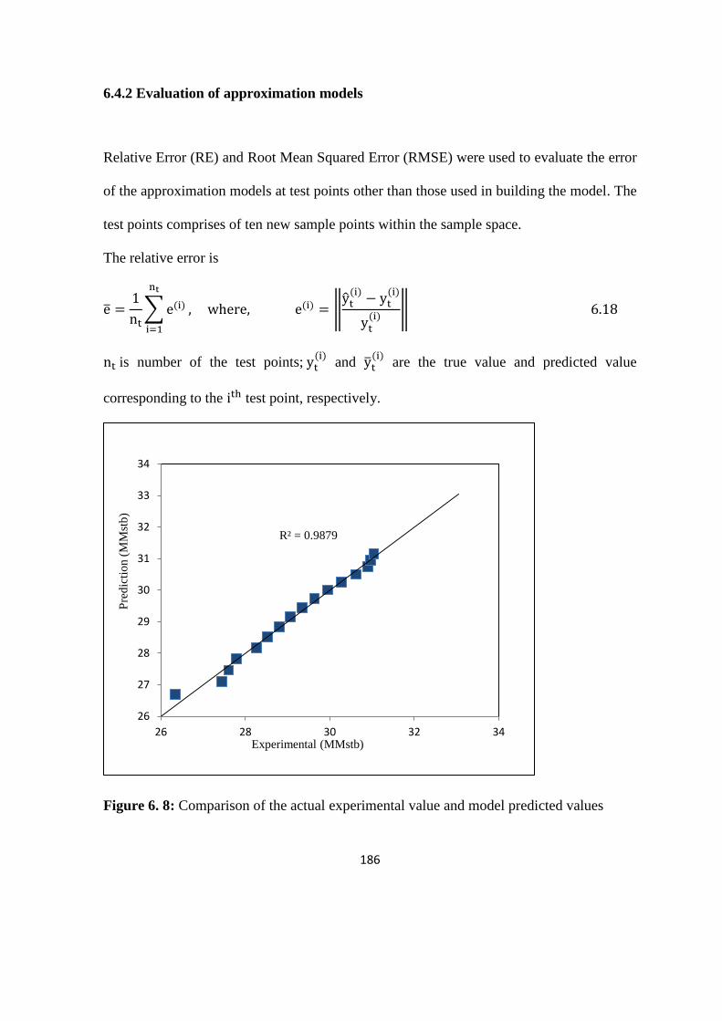
186
6.4.2 Evaluation of approximation models
Relative Error (RE) and Root Mean Squared Error (RMSE) were used to evaluate the error
of the approximation models at test points other than those used in building the model. The
test points comprises of ten new sample points within the sample space.
The relative error is
e =1
nt∑e(i)
nt
i=1
, where, e(i) = ‖yt
(i)− yt
(i)
yt(i)
‖ 6.18
nt is number of the test points; yt(i)
and yt(i)
are the true value and predicted value
corresponding to the ith test point, respectively.
Figure 6. 8: Comparison of the actual experimental value and model predicted values
R² = 0.9879
26
27
28
29
30
31
32
33
34
26 28 30 32 34
Pre
dic
tio
n (
MM
stb
)
Experimental (MMstb)
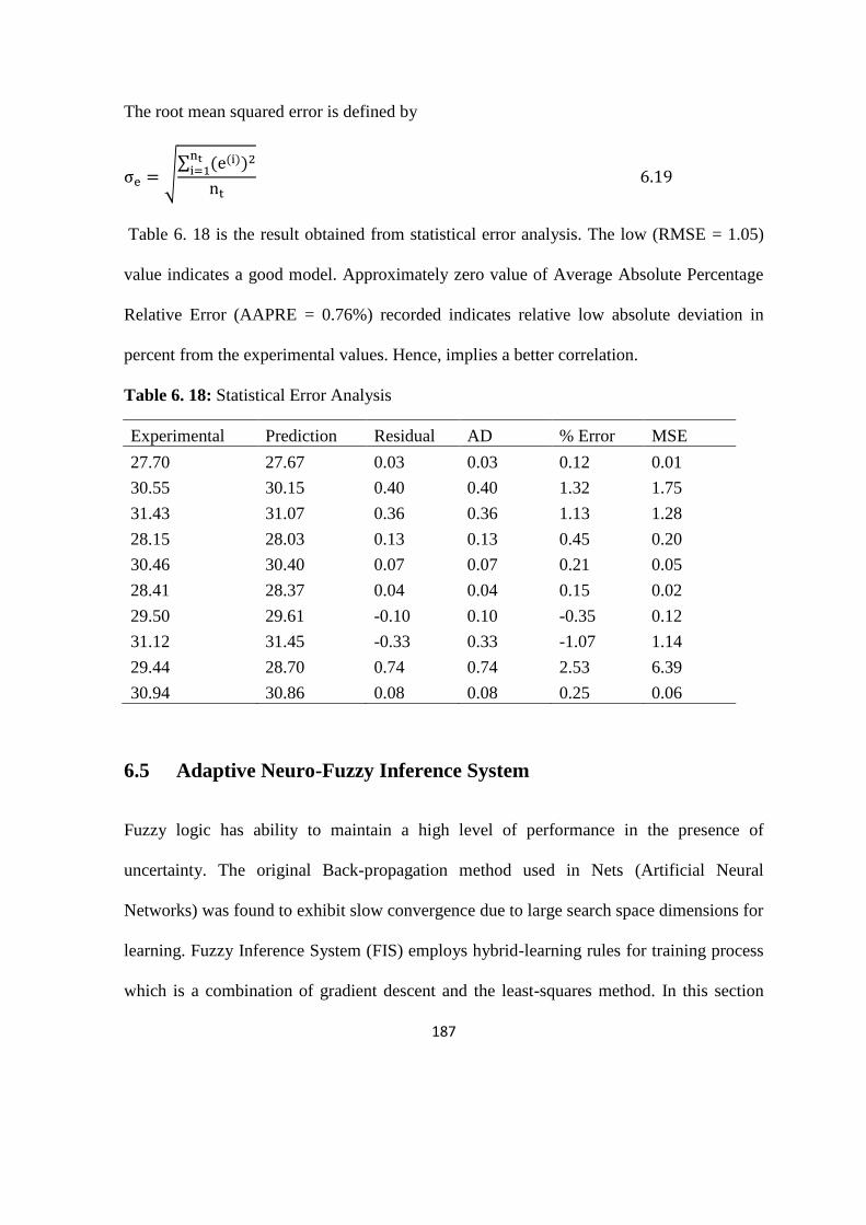
187
The root mean squared error is defined by
σe = √∑ (e(i))2nt
i=1
nt 6.19
Table 6. 18 is the result obtained from statistical error analysis. The low (RMSE = 1.05)
value indicates a good model. Approximately zero value of Average Absolute Percentage
Relative Error (AAPRE = 0.76%) recorded indicates relative low absolute deviation in
percent from the experimental values. Hence, implies a better correlation.
Table 6. 18: Statistical Error Analysis
Experimental Prediction Residual AD % Error MSE
27.70 27.67 0.03 0.03 0.12 0.01
30.55 30.15 0.40 0.40 1.32 1.75
31.43 31.07 0.36 0.36 1.13 1.28
28.15 28.03 0.13 0.13 0.45 0.20
30.46 30.40 0.07 0.07 0.21 0.05
28.41 28.37 0.04 0.04 0.15 0.02
29.50 29.61 -0.10 0.10 -0.35 0.12
31.12 31.45 -0.33 0.33 -1.07 1.14
29.44 28.70 0.74 0.74 2.53 6.39
30.94 30.86 0.08 0.08 0.25 0.06
6.5 Adaptive Neuro-Fuzzy Inference System
Fuzzy logic has ability to maintain a high level of performance in the presence of
uncertainty. The original Back-propagation method used in Nets (Artificial Neural
Networks) was found to exhibit slow convergence due to large search space dimensions for
learning. Fuzzy Inference System (FIS) employs hybrid-learning rules for training process
which is a combination of gradient descent and the least-squares method. In this section

188
experimental design and Adaptive Neuro Fuzzy Inference System (ANFIS) were integrated
to develop a predictive model for production forecast after infill drilling in a real Niger
Delta Field. Experimental design was employed for data gathering while ANFIS technique
was utilized for factor selection and predictive model development.
6.5.1 Data collection
Central Composite algorithm provides sufficient data within the design space for ANFIS
modelling. An overall of 145 experiments (Appendix D) were performed considering the
full factorial of CCD consisting of 128 cube points, 14 axial points, and 3 center points for
the seven screened “heavy-hitters”. Each factor was varied over five levels ±α (axial
points), ±1 (factorial points) and “0” (center-point). After data quality control, 143 valid
experimental points were used.
6.5.2 Data partitioning
Out of a total of 143 input–output pairs, 72% were randomly selected and used for training.
The remaining 28% of data were used for testing or validation. For training, the fuzzy rules
were generated directly from the input-output data sets and the model learnt the salient
features in the data and automatically adjusted the system parameters to reduce the error
between the predicted output and the measured output. The training was achieved using
genfis1 and the trainings of these networks were stopped after reaching the minimum error
goal of 0.0001 (MATLAB 2007 run on an Intel (R) Core (TM) i5 CPU (2.5 GHz, 6 GB
RAM) PC).

189
6.5.3 Optimization and selection of input parameters
Two optimization schemes were tested to reveal the inputs that have more impact on the
output, an exhaustive and sequential optimization schemes. Sequential search scheme
capable of selecting between 1 to 4 input variables from all input candidates and identifies
influence of variable and its interactions on model prediction. The search began with main
factor followed by 2-factors interaction, 3 factors interaction and 4 factors interaction.
Table 6. 19 shows how main factors and their interactions impacted the output for one
epoch number using RMSE criteria. The selection of the key factors was based on the
magnitude of RMSE of the training and data checking.
Table 6. 19: SEQSRCH results of “heavy-hitters” selection used for proposed model
development
RMSE
Uncertainty Training Testing
A 0.8020 0.8397
B 0.8631 0.8514
C 0.8638 0.8348
D 0.7554 0.7471
E 0.6270 0.7001
F 0.8237 0.8552
G 0.7642 0.7407
(EA) 0.5533 0.6571
(EB) 0.534 0.6318
(EC) 0.5058 0.6121
(ED) 0.5333 0.6399
(EF) 0.5528 0.6838
(EG) 0.4774 0.5559
(EGA) 0.3264 0.6446
(EGB) 0.3719 0.5642
(EGC) 0.3082 0.514
(EGD 0.3726 0.7366
(EGF) 0.3783 0.7315
(CEGA) 0.0682 0.9566
(CEGB) 0.1344 1.5383
(CEGD) 0.0998 1.5102
(CEGF) 0.1639 1.4011

190
A low training RMSE and significantly high checking RMSE is a sign of over-fitting.
Parameter E (training error of 0.6270 and checking error of 0.7001) is therefore selected
first ahead of remaining six main effects. For 2 interaction factors, EG with lowest training
and checking RMSE (0.4774 and 0.5559) was selected. The order of arrangement (EG and
not GE) also indicates the degree of significance of the two parameters with E having more
impact on the response than G. The selection process is similar for the other higher
combination of variables. Three (3) factors searching revealed EGC as having the closest
and lowest RMSE (0.3082 and 0.5140) values for training and checking errors. CEGA was
selected on searching for four factors with RMSE (0.0682 and 0.9566) for the training and
checking errors respectively. The selection process is similar for the other higher
combination of variables. Three (3) factors searching revealed EGC as having the closest
and lowest RMSE (0.3082 and 0.5140) values for training and checking errors. CEGA was
selected on searching for four factors with RMSE (0.0682 and 0.9566) for the training and
checking errors respectively.
6.5.4 Network architecture for ANFIS model
For the construction of ANFIS model, MATLAB toolbox was used. The training of the
ANFIS network was accomplished by employing grid partitioning to generate Fuzzy-
Inference System (FIS). FIS utilizes different membership functions. The membership
function assigned to each input was tuned using hybrid optimization method (which is a
combination of least squares method and gradient steepest descent method) for the
parameters associated with the input membership function and the least squares estimation
for the parameters associated with the output membership functions. A gradient vector was

191
used to measure how well the fuzzy system is modeling the input– output data. The fuzzy
inference system generated is shown in Figure 6. 9. The neuro-fuzzy structure is shown in
Figure 6. 10. Figure 6. 11 shows the rule for 4 Input Fuzzy Inference System and the
output panel. Figure 6. 12 shows error propagation from checking and training processes.
Figure 6. 13 shows the cross plot of actual and predicted values in ANFIS for training data
sets. Figure 6. 14 depicts the cross plot for the checking data versus model prediction for
the remaining 43 data set. Figure 6. 15 presents the parity plot of actual and predicted
values in ANFIS for all data sets.
6.5.5 Influence of membership function
Table 6.20 shows the different membership functions tested during modeling and they
influence the training and checking errors. Gaussian membership function (Gaussmf)
exhibited least over-fitting with R-square value of 96 percent. Figure 6. 9 consists of three
different parts: fuzzifiers, which map the crisp values of the preprocessed input of the
model into suitable fuzzy sets represented by membership functions; followed by the
inference mechanism or inference engine, which is the computational method to compute
the extent to which each rule fires for a given fuzzified input pattern according to an active
inference rule; and the last part is a defuzzifier, which maps the crisp values of the
preprocessed input of the model into suitable fuzzy sets represented by membership
functions and postprocessed to give the output of the fuzzy system based on the crisp
signal obtained after defuzzification.
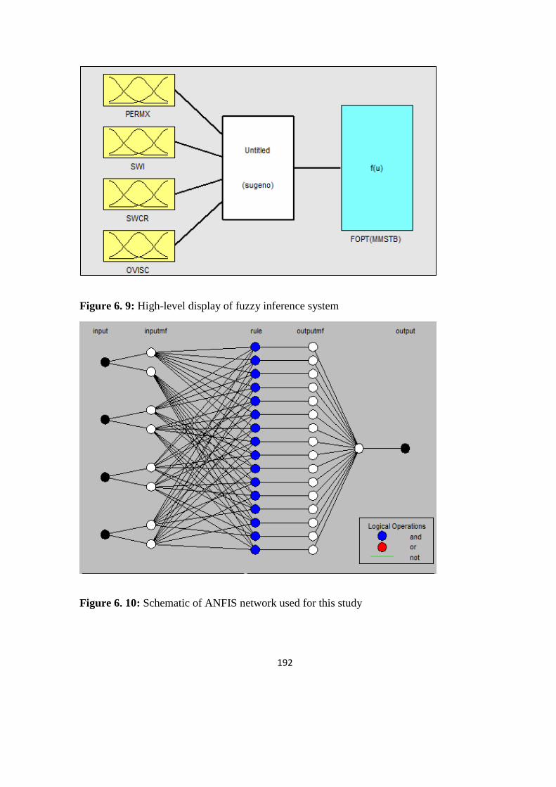
192
Figure 6. 9: High-level display of fuzzy inference system
Figure 6. 10: Schematic of ANFIS network used for this study

193
The neuro-fuzzy structure is shown in Figure 6. 10, which consists of 4 input nodes, 8
input membership function nodes, one node for normalized rules, one output membership
node, and one output node.
Figure 6. 11: Panel showing Rule for 4 Input Fuzzy Inference System

194
Table 6. 20: Influence of different Membership Function
Figure 6. 12: Error propagation for checking (upper) and training (lower).
RMSE Error
MF Training Checking R-Square Value
Gbell 0.215383 0.324773 0.95471
Gauss 0.22372 0.304382 0.956
Gauss2 0.21318 0.323268 0.95545
Tri 0.221813 0.302415 0.95673
Pi 0.198293 0.350266 0.95415
Psig 0.223396 0.353501 0.9486
Dsig 0.223396 0.353501 0.9486

195
It is evident from Figure 6. 12 that as the training error decreased from 0.264917 to
0.22372, the checking error reduced up to epoch number of about 18 and shoot up gently
indicating occurrence of minimum over-fitting before it stabilized. Over-fitting was
checked by selecting appropriate membership function that associated with the minimum
checking error.
Figure 6. 13: Parity plot of Actual and predicted values in ANFIS for training data sets.
Figure 6. 13 is the cross plot of the trained 100 data set versus model prediction for the first
100 epoch number. The model intersected most of the data point with correlation
coefficient of 93 percent.
R² = 0.9295
19
19.5
20
20.5
21
21.5
22
22.5
23
23.5
24
19 20 21 22 23 24
Pre
dic
ted
Val
ue
(M
Mst
b)
Actual Value (MMstb)

196
Figure 6. 14: Parity plot of Actual and predicted values in ANFIS for checking data sets.
Figure 6. 14 depicts the cross plot for the checking data versus model prediction for the
remaining 43 data set. The prediction coefficient is 0.8455 and the root mean square error
is 4%.
R² = 0.8455
16
17
18
19
20
21
22
23
24
16 18 20 22 24
Pre
dic
ted
Val
ue(
MM
stb
)
Actual Value (MMstb)
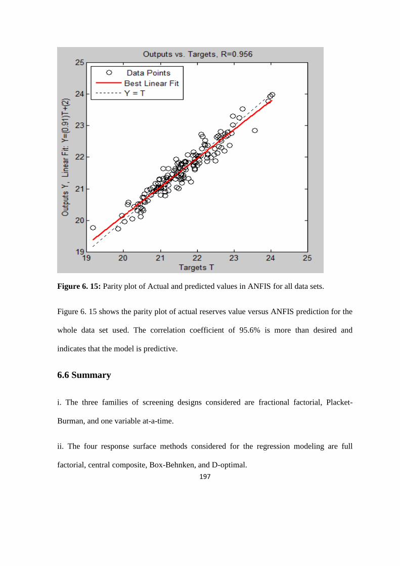
197
Figure 6. 15: Parity plot of Actual and predicted values in ANFIS for all data sets.
Figure 6. 15 shows the parity plot of actual reserves value versus ANFIS prediction for the
whole data set used. The correlation coefficient of 95.6% is more than desired and
indicates that the model is predictive.
6.6 Summary
i. The three families of screening designs considered are fractional factorial, Placket-
Burman, and one variable at-a-time.
ii. The four response surface methods considered for the regression modeling are full
factorial, central composite, Box-Behnken, and D-optimal.

198
iii. A total of 9 response surface models developed were validated and subjected to
statistical error analysis.
iv. In all screening methods, years of production forecast played important role on
associated number of “heavy-hitters.” A full 2-level factorial or high resolution fractional
factorial method was equally adequate for the construction of response surfaces for
uncertainty quantification where 3-level full factorial was not feasible. Uniform design
(UD) of experiment was also used to provide alternative to all conventional designs.
vi. Experimental design and Numerical simulation were integrated to develop ANFIS
based proxy model for the production forecast. The prediction from the ANFIS model
gives a better prediction and accuracy (AAPRE of 0.7406 and R-square of 0.956) than the
response surface models (AAPRE of 2.913 and 0.8819) usually developed from the
analysis of experimental design.
ANFIS model utilized fewer parameters when compare with RSM based proxy-model and
therefore offers more flexibility where data availability poses serious challenge.

199
Chapter 7
7. Uncertainty Quantification
Two Monte Carlo methods were compared on the basis of underlying assumptions that
characterizes them for quantifying uncertainty in reservoir forecast.
7.1 The Ordinary Monte Carlo simulations
The term Monte Carlo indicates all those stochastic algorithms using the central limit
theorem to compute multidimensional integrals. Numerical solution of a D–dimensional
integral with a relative accuracy ϵ requires a computation time proportional to ϵ-D
.
However, with the central limit theorem, Monte Carlo methods scale as ϵ-2
, regardless of
the dimensionality. Consequently, a surprising number of statistical problems utilize Monte
Carlo techniques. Apart from this, numerical methods often give perfectly ‘deterministic’
results.
Whether or not the Monte Carlo method can be applied to a given problem does not
depend on the stochastic nature of the system being studied, but only on our ability to
formulate the problem in such a way that random numbers may be used to obtain the
solution. Every application of the Monte Carlo method can be represented as a definite
integral:
I = ∫ f(x)dx
Ω
7.1
200
Where domain Ω is a region in multiple-dimensional space and f(x) is the integrand. The
idea is to estimate the integral with an expected value using random samples. Integral I can
be interpreted as the expected value of random variable f(X), where x is an independent
random variable and identically distributed (iid) usually, uniformly distributed in Ω.
If we draw a set of samples, 𝑥1, … , 𝑥𝑛 uniformly in Ω, then an approximation to I can be
obtained by its arithmetic mean:
IN =1
N∑f(Xi)
N
i=1
7.2
Generally, we often possess a probability distribution, π, from which we want to determine
a point-estimate. However, scientific facts are usually presented in the media through the
first moment, the mean, even though such an estimate rarely reflects the actual structure of
π. Such an estimate can be determined through the following expression for any suitable
function g:
π(g) = Eπ[g(X)] = ∫g(x)π(dx) 7.3
E
In most practical cases, analytic calculation of 𝜋(𝑔) in equation 7.3 is rarely possible. So,
approximate answer is usually demanded. In order to determine such estimates one has to
resort to an approximation.
7.1.1 Framework for integral computation
For a generic real function 𝑓(𝑥) of dimension D, we can compute the integral as follows:
∫f(x )dDx = ∫f(x )
p(x )p(x )dDx 7.4
= ∫g(x )p(x )dDx 7.5

201
With
g(x ) =f(x )
p(x )
and we can use the central limit theorem to write the estimate
∫f(x )dDx ≈ SN ± σN
Central limit theorem
Let 𝑥𝑖 be a sequence of stochastic D–dimensional independent variables distributed with
a probability density 𝑝(𝑥 ), and 𝑓(𝑥 ) a real function. For the function, in accordance with
the law of large number,
SN ≡1
N∑f(xi )
N
i=1
7.6
Central limit theorem states that the probability density 𝑆𝑁 in the large N limit can be
written as
limN→+∞
P(SN) =1
√2πσN2
e−
(SN−<f>)2
2σN2
7.7
Where
< f >≡ ∫ f(x )p(x )dDx 7.8
< f2 >≡ ∫ f2(x )p(x )dDx 7.9
σN2 =
< f2 > −< f >2
N 7.10
In other words SN is an estimate of < f > and σN is its variance.
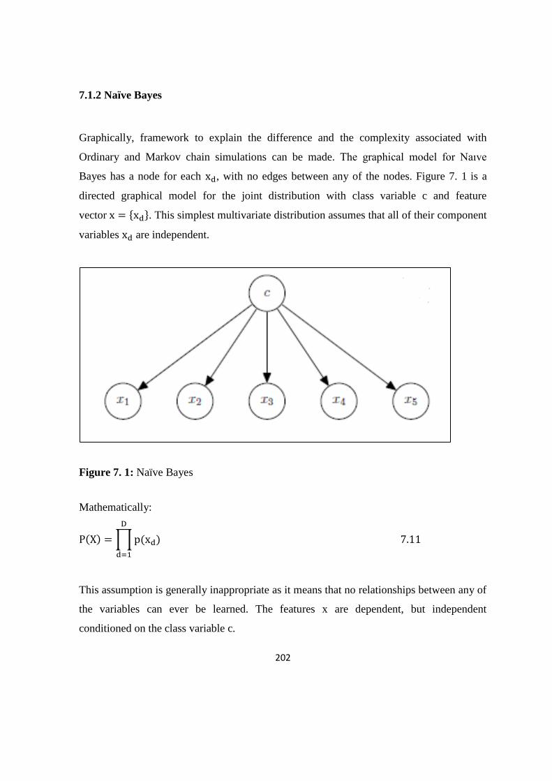
202
7.1.2 Naïve Bayes
Graphically, framework to explain the difference and the complexity associated with
Ordinary and Markov chain simulations can be made. The graphical model for Naıve
Bayes has a node for each xd, with no edges between any of the nodes. Figure 7. 1 is a
directed graphical model for the joint distribution with class variable c and feature
vector x = xd. This simplest multivariate distribution assumes that all of their component
variables xd are independent.
Figure 7. 1: Naïve Bayes
Mathematically:
P(X) = ∏p(xd)
D
d=1
7.11
This assumption is generally inappropriate as it means that no relationships between any of
the variables can ever be learned. The features x are dependent, but independent
conditioned on the class variable c.
203
7.1.3 Assumption in OMCS
Independence of two measurable sets implies that any information about an event
occurring in one set has no information about whether an event occurs in another set. If we
let X1 and X2 to be two events in the sample space, then X1 and X2 are independent if and
only if
Pr(X1 ∩ X2) = Pr(X1)Pr(X2) 7.12
One immediate implication of the definition of independence is that when
X1 and X2 independent, the conditional probability of one given the other is the same as the
unconditional probability of the random variable:
Pr(X1 X2⁄ ) = Pr(X1) 7.13
Let us consider two random variables x and y. In order to specify completely the
distribution of x and y, we now requires an approximation function of the two variables
say:
h(x, y) = ax + b 7.14
This ensuing mathematics can be more complicated. However, when the function h(x, y)
can be factored exactly into a product of two functions, each of the variable depends only
on one variable, we say that x and y are stochastically independent since the distribution of
x does not depend on the value of y and vice versa.
h(x, y) = p(x)q(y) 7.15
When more than two variables are considered, the concept of independence becomes more
complicated, and it is no longer sufficient to consider only the dependence of pairs of

204
variables. Indeed, it is possible to have all pairs of variables independent and still have
dependence among triplets or higher combinations of variables.
The solution of the integral always requires the estimation of probability and cumulative
density functions (pdf and cdf). Those probability density functions have to be determined
by trial-and-error while performing Monte Carlo simulation. Consider a separable
multivariable function:
f(k, ∅) = g(k)h(∅) 7.16
The probability density function as a function of one of the variables can be found by
separation as shown in Equations 7.17 through 7.20.
P(k) =∫ f(k, ∅)d∅
∅max
∅min
∫ ∫ f(k, ∅)dkd∅∅max
∅min
kmax
kmin
7.17
P(k) =g(k) ∫ h(∅)d∅
∅max
∅min
∫ g(k)dk ∫ h(∅)d∅∅max
∅min
kmax
kmin
7.18
P(k) =g(k)
∫ g(k)dkkmax
kmin
7.19
P(∅) =h(∅)
∫ h(∅)d∅∅max
∅min
7.20
For non-separable functions
h(k, ∅) = ak + b∅2 7.21
The Marginal Density Functions can be found as identified in Equations 7.22.
R(k) = ∫ ∫ P(k, ∅)d∅dk∅max
∅min
k
−∞
7.22
Suppose X is a bivariate random variable with probability density function

205
f(k, ∅) = ak + b∅2 7.23
defined on [0, 1] x [0, 1]. Then the associated cdf is
F(k, ∅) = ∫∫(ak + b∅2)dkd∅ 7.24
= a2⁄ k2∅ + b
3⁄ k∅3 7.25
7.1.4 Relationship between CDF and PDF
Let f(x1, … , xn) and F(x1, … , xn) represent the pdf and cdf of an n − dimensional con −
tinuous random variable X, respectively. the density function for X can be defined as
f(x1, … , xn) =∂nF(X)
∂x1 ∂x2 …∂xn 7.26
wherever f(x1, … , xn) is continuous and f(x1, … , xn) = 0 elsewhere.
Suppose X is a bivariate random variable with cumulative distribution function
F = a2⁄ k2∅ + b
3⁄ k∅3
The probability density function can be determined thus:
f(x1, … , xn) =∂2F(k, ∅)
∂k∂∅
=∂
∂∅(ak∅ + b
3⁄ ∅3)
= ak + b∅2
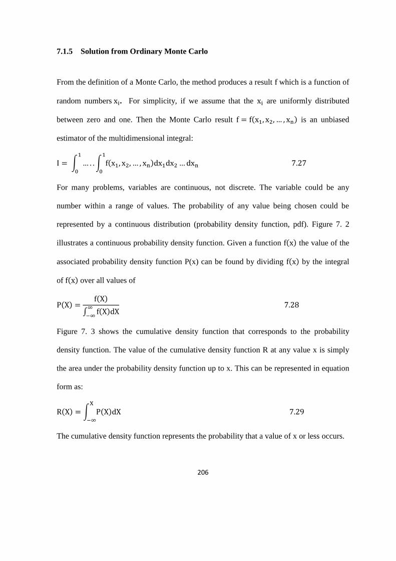
206
7.1.5 Solution from Ordinary Monte Carlo
From the definition of a Monte Carlo, the method produces a result f which is a function of
random numbers xi. For simplicity, if we assume that the xi are uniformly distributed
between zero and one. Then the Monte Carlo result f = f(x1, x2, … , xn) is an unbiased
estimator of the multidimensional integral:
I = ∫ … . .∫ f(x1, x2, … , xn)dx1dx2 …dxn
1
0
1
0
7.27
For many problems, variables are continuous, not discrete. The variable could be any
number within a range of values. The probability of any value being chosen could be
represented by a continuous distribution (probability density function, pdf). Figure 7. 2
illustrates a continuous probability density function. Given a function f(x) the value of the
associated probability density function P(x) can be found by dividing f(x) by the integral
of f(x) over all values of
P(X) =f(X)
∫ f(X)dX∞
−∞
7.28
Figure 7. 3 shows the cumulative density function that corresponds to the probability
density function. The value of the cumulative density function R at any value x is simply
the area under the probability density function up to x. This can be represented in equation
form as:
R(X) = ∫ P(X)dXX
−∞
7.29
The cumulative density function represents the probability that a value of x or less occurs.
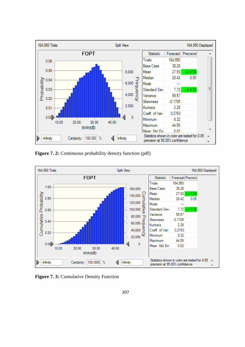
207
Figure 7. 2: Continuous probability density function (pdf)
Figure 7. 3: Cumulative Density Function

208
7.1.6 Risk curves using OMCS
The Monte Carlo technique was used to combine the uncertain attributes using response
surface equations developed in chapter 6. Two thousand (2000) iterations were made while
assumed the following distribution functions: triangular for OVISC, uniform for PORO,
Log normal for PERMX and PERMZ, Normal for SWC, triangular for AQUIPV and
triangular for KRW.
It was found that 2000 equiprobable realisations iteratively built in Excel were enough to
stabilize the resulting forecast distributions. One critical measure used to generate each
realisation of the model is that the deterministic reserve value was fairly maintained at
simulation base case value throughout the process. Cumulative probability distribution for
the forecast reserves are shown in Figure 7. 4 through Figure 7. 6. The impact of the major
uncertain parameters was quantified.
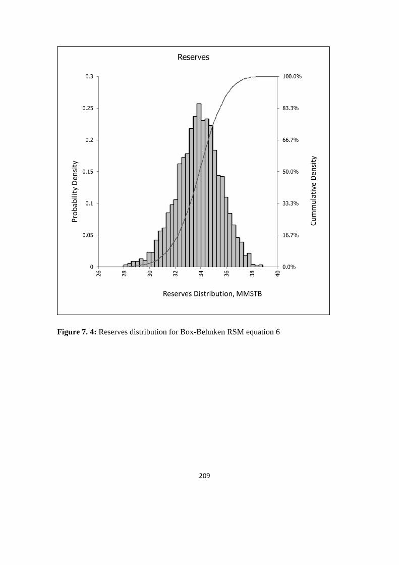
209
Figure 7. 4: Reserves distribution for Box-Behnken RSM equation 6
0.0%
16.7%
33.3%
50.0%
66.7%
83.3%
100.0%
0
0.05
0.1
0.15
0.2
0.25
0.3
26
28
30
32
34
36
38
40
Cu
mm
ula
tive
Den
sity
Pro
bab
ility
Den
sity
Reserves Distribution, MMSTB
Reserves
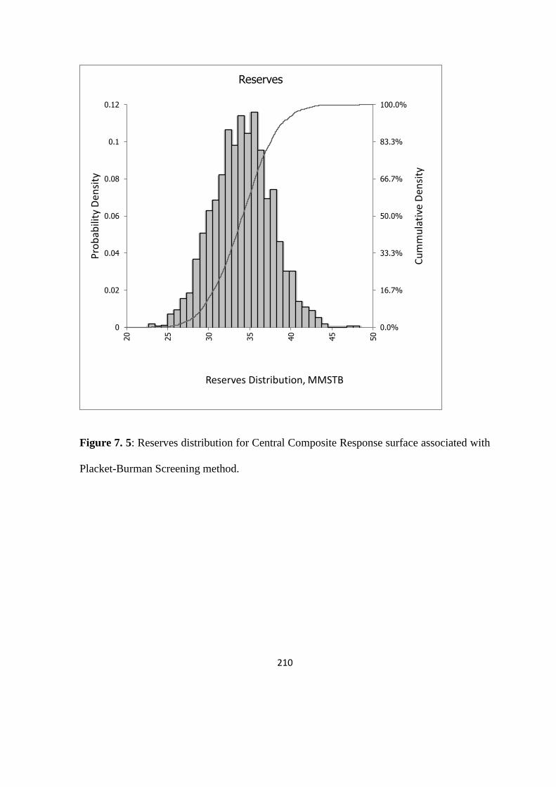
210
Figure 7. 5: Reserves distribution for Central Composite Response surface associated with
Placket-Burman Screening method.
0.0%
16.7%
33.3%
50.0%
66.7%
83.3%
100.0%
0
0.02
0.04
0.06
0.08
0.1
0.12
20
25
30
35
40
45
50
Cu
mm
ula
tive
Den
sity
Pro
bab
ility
Den
sity
Reserves Distribution, MMSTB
Reserves
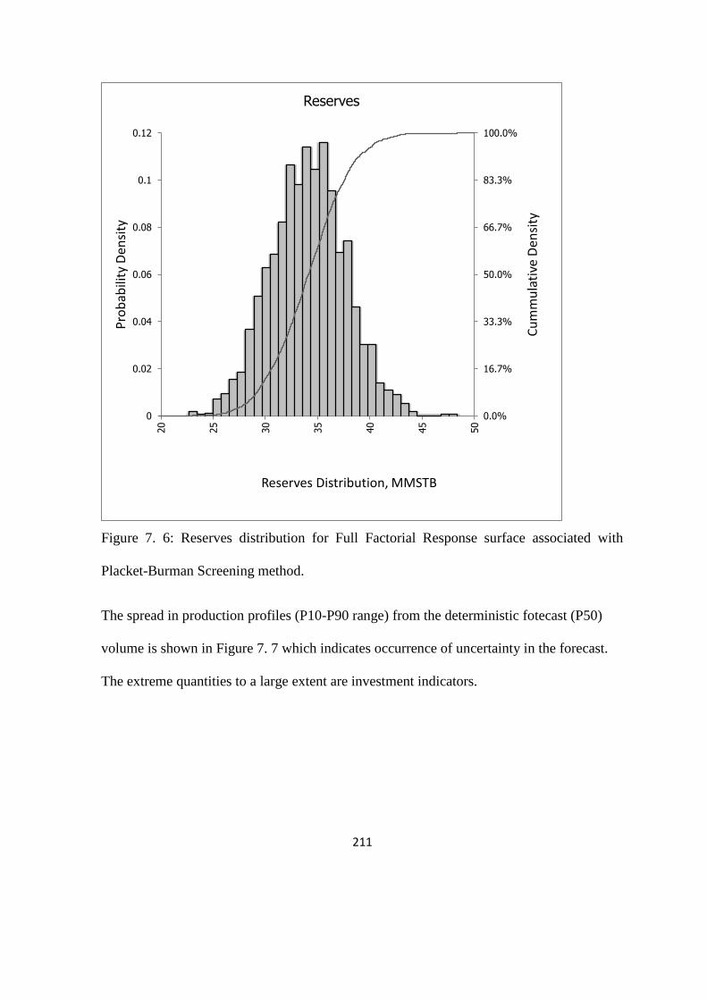
211
Figure 7. 6: Reserves distribution for Full Factorial Response surface associated with
Placket-Burman Screening method.
The spread in production profiles (P10-P90 range) from the deterministic fotecast (P50)
volume is shown in Figure 7. 7 which indicates occurrence of uncertainty in the forecast.
The extreme quantities to a large extent are investment indicators.
0.0%
16.7%
33.3%
50.0%
66.7%
83.3%
100.0%
0
0.02
0.04
0.06
0.08
0.1
0.12
20
25
30
35
40
45
50
Cu
mm
ula
tive
Den
sity
Pro
bab
ility
Den
sity
Reserves Distribution, MMSTB
Reserves
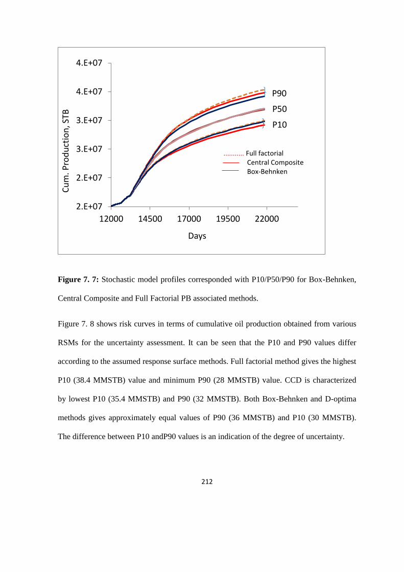
212
Figure 7. 7: Stochastic model profiles corresponded with P10/P50/P90 for Box-Behnken,
Central Composite and Full Factorial PB associated methods.
Figure 7. 8 shows risk curves in terms of cumulative oil production obtained from various
RSMs for the uncertainty assessment. It can be seen that the P10 and P90 values differ
according to the assumed response surface methods. Full factorial method gives the highest
P10 (38.4 MMSTB) value and minimum P90 (28 MMSTB) value. CCD is characterized
by lowest P10 (35.4 MMSTB) and P90 (32 MMSTB). Both Box-Behnken and D-optima
methods gives approximately equal values of P90 (36 MMSTB) and P10 (30 MMSTB).
The difference between P10 andP90 values is an indication of the degree of uncertainty.
2.E+07
2.E+07
3.E+07
3.E+07
4.E+07
4.E+07
12000 14500 17000 19500 22000
Cu
m. P
rod
uct
ion
, STB
Days
P90
P50
P10
........... Full factorial Central Composite Box-Behnken

213
Figure 7. 8: Impact of different RSMs on Uncertainty assessment
The risk curves generated from MCS provide information on the risk associated with
wanton adoption of experimental designs for response surface methodology. The figure
clearly shows the uncertainties associated with the choice of percentiles for investment
decision. The costs and benefits of conducting additional experiments due to preference for
one design method relative to others are also highlighted in Figure 7. 8.
0
0.1
0.2
0.3
0.4
0.5
0.6
0.7
0.8
0.9
1
25 30 35 40 45 50
PER
CEN
TILE
Reserves, MMSTB
Central Composite
Full Factorial
D-Optima
Box-Behnken
38.4MMSTB
36MMSTB
35.4MMSTB

214
Figure 7. 9: Risk Curves for Case 1 – (a) Box-Behnken equations 6.2, 6.6 and 6.10 (b)
Central Composite equations 6.3 and 6.9 (c) Full Factorial equations 6.5 and 6.7
The implication of performing 46 and 62 experiments using fractional and relative
variation designs respectively instead of the 29 using PB design was examined by
constructing a multiple risk curves. For the curves, P50 values are ensured equal after MCS
as shown in Figure 7. 9. A good agreement of risk curves of Box-Behnken associated with
Placket-Burman and fractional factorial screening designs. The same applied to full
factorial risk curves shown in Figure 7. 9c. However, the risk curve associated with
screening using the one variable at-a-time exhibits wider variability from others and tends

215
to be more optimistic which is perhaps due to different occurrence probability and larger
number of factors involved in the regression analysis. The risk curves obtained by CCD
developed from Placket-Burman and fractional factorial is a little at variance from each
other due to combination that possesses dissimilar occurrence probability. In summary,
both fractional screening design and PB design tend to give approximate result. Based on
the analysis, there is no significant added advantage in performing 46 experiments as
required by fractional factorial screening method. PB with fewer experimental runs is
therefore desirable.
7.2 Markov Chains Model
The arrow directions make a big difference in Figure 7.10 compare with Figure 7.1. The x
variables are independent in the generative process.
Figure 2: Hidden causes
After observing y our knowledge about x forms a potentially complex joint distribution.
Ordinary Monte Carlo approach can-not be used here because we do not expect direct

216
sampling from 𝑝(𝑥 𝑦⁄ ) to be easy. Methods based on Markov chains will offer a solution to
this problem.
Mathematically,
p(y, X) = p(y)p(X y⁄ ) = p(y)∏p(xd
y⁄ )
D
d=1
7.2.1 Uncertainty quantification
Bayesian approach, expresses uncertainties in the model’s parameters θ in terms of
probability. Parameter uncertainty is quantified first by introducing a prior probability
distribution 𝑃(𝜃), which represents the knowledge about θ before collecting any new data,
and second, by updating this prior probability on θ to account for the new data collected
(D).
This updating is performed using Bayes’ theorem, which can be expressed as:
P(D θ⁄ ) =P(D θ⁄ ). P(θ)
∫ P(D θ⁄ ). P(θ). dθ 7.30
Where 𝑃(𝜃 𝐷⁄ ) is the posterior distribution of 𝜃; ∫𝑃(𝐷 𝜃⁄ ). 𝑃(𝜃)𝑑𝜃 is a normalizing
constant required so that ∫ 𝑃(𝐷 𝜃⁄ ). 𝑑𝜃 = 1, and 𝑃(𝐷 𝜃⁄ ) is the conditional probability for
the measured data given the parameters. 𝑃(𝐷 𝜃⁄ ) is often referred to as the likelihood
function.
7.2.2 The advantage of Bayesian Monte Carlo method
Bayesian methods explicitly use probability distributions as a way to quantify uncertainties
about the unknown quantities. The inference is carried out conditional on the observed data

217
and unlike OMCS, it does not rely on the assumption that a hypothetical infinite population
of data exists. This quality gives certain advantages to Bayesian methods over ordinary
Monte Carlo; such as that all inferences are exact and not approximated and that the results
are interpretable so that one can easily answer any scientific questions directly.
However, no readily available asymptotic results (such as the central limit theorem based
on an asymptotic increment of data) can be used to facilitate estimations, and Bayesian
analysis usually requires a much greater amount of computational resources.
7.2.3 Markov simulation
With MCMC, we sample from the posterior directly, and obtain sample estimates of the
quantities of interest, thereby performing the integration implicitly. Suppose that we have
some distribution 𝜋(𝑥), 𝑥 ∈ 𝐸 ∁ 𝑅𝑝, which is known only up to some multiplicative
constant. We commonly refer to this as the target distribution. If 𝜋 is sufficiently complex
that we cannot sample from it directly, an indirect method for obtaining samples from 𝜋 is
to construct an aperiodic and irreducible Markov chain with state space E, and whose
stationary (or invariant) distribution is 𝜋(𝑥), as discussed in Smith and Roberts (1993).
Then, if we run the chain for sufficiently long, simulated values from the chain, can be
treated as a dependent sample from the target distribution and used as a basis for
summarizing important features of π. A brief description of the implementation of MCMC
algorithm in a general setting is given here. Let us define
X = (x1, x2, … , xn)T
as an observed sample of size n from the univariate distribution f(x θ⁄ ). Here the parameter
θ is a vector containing p elements,

218
θ = (ϑ1, ϑ2, … , ϑp)T.
We assume the parameters are conditionally independent and the prior distribution of
θj is Pj(θj), for j = 1,2, … , p. Therefore the likelihood function L(X θ⁄ ) takes the form
L(X θ⁄ ) = ∏f(xi θ⁄ )
n
i=1
7.31
The joint posterior distributions of the parameter vector up to the normalizing constant is
P(θ X⁄ ) ∝ ∏f(xi θ⁄ ).∏Pj(θj) 7.32
p
j=1
n
i=1
Except in a few cases, the posterior distribution in equation 7.32 cannot be evaluated.
However, the Metropolis-Hastings (MH) method prescribes a way to simulate the posterior
distribution. We describe the algorithm in the following manner.
Step 1 Specify the initial guess of the parameter vector θ0 (for example this could be the
modes of each of the prior distributions).
Step 2 Specify proposal distributions, qj(θj θ⁄ ) for each of the parameters θj for j =
1,2, … , p.
Step 3 MCMC Simulation
For t from 1 to B + N do /∗ B simulations are burn − in ∗/
Let θt = [θ1t , θ2
t , … , θpt ]
For j from 1 to p do
Simulate θj∗ from qj(θ θj
t−1⁄ )
Let θj∗t = [θ1
t , θ2t , … , θj
∗, θj+1t−1, θj+2
t−1, … , θpt−1]

219
Let r =P(θj∗
t X⁄ )qj(θjt−1 θj
∗⁄ )
P(θt−1 X⁄ )qj(θj∗ θj
t−1⁄ )
Simulate U from Uniform[0,1]
Set θjt =
θj∗ if U < min(r, 1)
θjt−1 otherwise
end do
if t > B then
Simulate xt−Bpred
from f(x θt⁄ )
end if
end do
Step 3 Simulate observations from the predictive distributions after a certain number of
burn-ins. At the end we could construct the empirical distribution based on the simulated
sample x1pred
, x2pred
, … , xNpred
and this would be the predictive distribution (Gilks et al.,
1996).
7.2.4 Metropolis algorithm
Although the Metropolis algorithm is not the most efficient Markov Chain sampler, it is
chosen in this study because of the simplicity of its implementation, and its generality. It
only requires knowledge about the likelihood function to update simultaneously the
parameters set for each iteration. Supposing that residuals between model and observation
are N(0, σ2), the likelihood function can be written in the multiplicative form:
P(D θ⁄ ) = ∏1
(2. π. σ2)1
2⁄. e
(Yt−f(Xt,θ))2
2.σ2 7.33
n
t=1

220
Where (𝑌1 … . 𝑌𝑛) is the vector of the measured response Y, (𝑌1 … . 𝑌𝑛) is a vector of input
data, 𝜃 = (𝜃1, … , 𝜃𝑝) is the vector of p unknown parameters, and 𝑓( ) is the model’s
output. σ is considered, as well as θ, as a set of parameters to be estimated during
calibration.
At each iteration, candidate values of parameters are drawn from a multi-normal transition
probability distribution for which the variance could be tuned up in a way to increase the
speed of convergence. However, updating periodically (automatically) the variance during
the simulation, is difficult. This was handled by fixing a prior value of the variance
according to the information about the parameters during all the simulation (Kuczera and
Parent, 1998).
An interesting feature of the Metropolis algorithm is that the interaction among the
model’s parameters is reflected in the likelihood function, so there will be no need to
incorporate correlation in the prior distributions of parameters. In order to avoid favoring
any initial value, a uniform prior distribution was used over the range of parameters.
7.3 Monte Carlo Application to Case Study
7.3.1 Surrogate Model
The reservoir described in chapter 5 as case study 2 was used to illustrate the differences
between the Ordinary and Bayesian Monte Carlo simulations. The first task was to develop
a mathematical function that approximates the observations (cumulative production) after
running the flow simulation over 25 years. The following assumptions are considered:
1. A data set X ∈ Rn,s, y ∈ Rn is provided
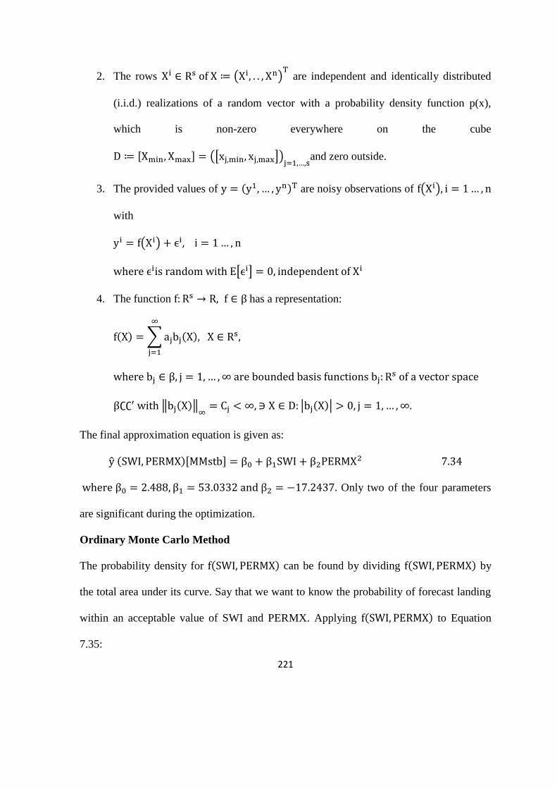
221
2. The rows Xi ∈ Rs of X ≔ (Xi, . . , Xn)T are independent and identically distributed
(i.i.d.) realizations of a random vector with a probability density function p(x),
which is non-zero everywhere on the cube
D ≔ [Xmin, Xmax] = ([xj,min, xj,max])j=1,…,sand zero outside.
3. The provided values of y = (y1, … , yn)T are noisy observations of f(Xi), i = 1… , n
with
yi = f(Xi) + ϵi, i = 1… , n
where ϵiis random with Ε[ϵi] = 0, independent of Xi
4. The function f: Rs → R, f ∈ β has a representation:
f(X) = ∑ajbj(X), X ∈ Rs,
∞
j=1
where bj ∈ β, j = 1, … ,∞ are bounded basis functions bj: Rs of a vector space
β∁∁′ with ‖bj(X)‖∞
= Cj < ∞, ∋ X ∈ D: |bj(X)| > 0, j = 1, … ,∞.
The final approximation equation is given as:
y (SWI, PERMX)[MMstb] = β0 + β1SWI + β2PERMX2 7.34
where β0 = 2.488, β1 = 53.0332 and β2 = −17.2437. Only two of the four parameters
are significant during the optimization.
Ordinary Monte Carlo Method
The probability density for f(SWI, PERMX) can be found by dividing f(SWI, PERMX) by
the total area under its curve. Say that we want to know the probability of forecast landing
within an acceptable value of SWI and PERMX. Applying f(SWI, PERMX) to Equation
7.35:

222
P(X, Y) =f(X, Y)
∫ ∫ f(X, Y)dXdYy2
y1
x2
x1
7.35
where X = SWI and Y = PERMX
Knowing the probability distribution, it is necessary to randomly draw uniformly
distributed numbers between x1 to x2, and y1 to y2. In reality, computer programs with
random number generators develop pseudorandom numbers. The pseudo-random numbers
that are drawn independently are assigned as variables x1 and y1. These variables does not
obey the intended probability density function though, it obeys a uniform distribution. To
ensure that x1 and y1 obey the distribution identified by Equation 7.35, input x1 and y1
into P(X, Y). This will result in a value P(x1, y1). Now draw another pseudo-random
number between 0 and 1, which will be called P2. If P(x1, y1) is less than P2, then a
realistic forecast is made at(x1, y1). If not, the value chosen for (x1, y1) should be rejected
and another attempt at selecting (x1, y1) should be made. The rejections result in a
distribution for (x1, y1) that obeys P(X, Y). The obvious disadvantage of forcing (x1, y1) to
obey the selected probability distribution is that there will be a lot of rejections at higher
(x1, y1) resulting in longer computational time. A method of identifying (x1, y1) that
makes more sense computationally is to utilize the cumulative distribution function.
The cumulative distribution function that corresponds to Equation 7.31 can be found by the
application of Equation 7.29 extended to two variables X and Y is given as:
R(X, Y) = ∫ ∫ P(X, Y)dXdY∞
−∞
∞
−∞
7.36
The cumulative density function given by Equation 7.36 accounts for the distribution of the
probability density function over all values of x and y. Because of this, no rejections are

223
required in order to use the cumulative density function to generate values of (x1, y1). It is
for this reason that most Monte Carlo codes utilize the cumulative density function rather
than the probability density function to generate simulated variables. To use the cumulative
density function to determine x and y, a uniformly distributed number between 0 and 1
should be drawn using a pseudo-random number generator. This value is substituted for
R(X, Y) independently, and x and y can then be solved for using Equation 7.36.
However, by using Equation 7.34 and substituting in, the mid values for SWI (0.65-0.9) of
0.775 and PERMX (0.57-1.3) of 0.935, the forecast is analytically determined to be
28.54MMstb by direct substitution.
Assuming uniform parameter distribution, the 500, 1000, 2500, 3500, 5000 and 10000
trials, for the Monte Carlo using Crystal Ball produces the mean forecast shown in Table
7.1.
Because the results for the forecasts are determined based on a number of trials and have
some variability, 10 trials for each sample size were performed so as to be able to assess
the mean and variance. The means, standard deviations, and variances are also reported in
Table 7.1 along with the forecasts for each sample size. It is possible to make some
observations from the data. Note that as the sample size increases, the standard deviation
and variance are reduced. Additionally, larger sample sizes tend to result in mean forecast
that are closer than for smaller sample sizes. The results compare well with the
deterministic value of 28.54MMstb. Even for 1000 trials, the difference between the
deterministic forecast and the mean Monte Carlo determined forecast value was only
1.92%.

224
The cumulative and density functions from the Crystal ball are presented as shown in
Figure 7.10 and Figure 7.11 as cdf and pdf respectively. The distribution of forecast at 5%
increment with corresponding values of parameter is also presented in Table 7. 2.
Table 7. 1: Results for uncertainty quantification for forecast problem
Size 500 1000 2500 3500 5000 10000
Run
1 28.23 28.02 27.91 27.76 27.82 27.95
2 28.16 28.13 27.86 27.93 28 27.96
3 27.72 28.34 27.67 28.02 27.9 27.93
4 27.3 27.53 28.01 27.85 28.05 27.95
5 28.16 28.01 27.85 27.79 27.92 27.99
6 27.95 28.33 27.88 27.77 27.99 27.95
7 27.91 27.34 27.78 27.86 27.86 27.95
8 27.24 28.13 27.71 27.93 27.89 27.96
9 27.93 27.98 27.82 28.04 27.92 27.96
10 27.85 28.1 27.76 27.81 27.9 27.98
Mean 27.845 27.991 27.825 27.876 27.925 27.958
St. Dev 0.341215149 0.320570672 0.099916632 0.100465583 0.069322114 0.016865481
Variance 0.104785 0.092489 0.008985 0.009084 0.004325 0.000256
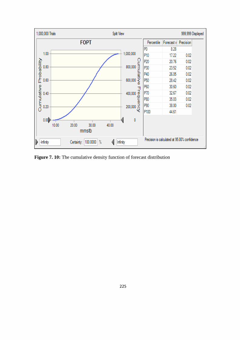
225
Figure 7. 10: The cumulative density function of forecast distribution
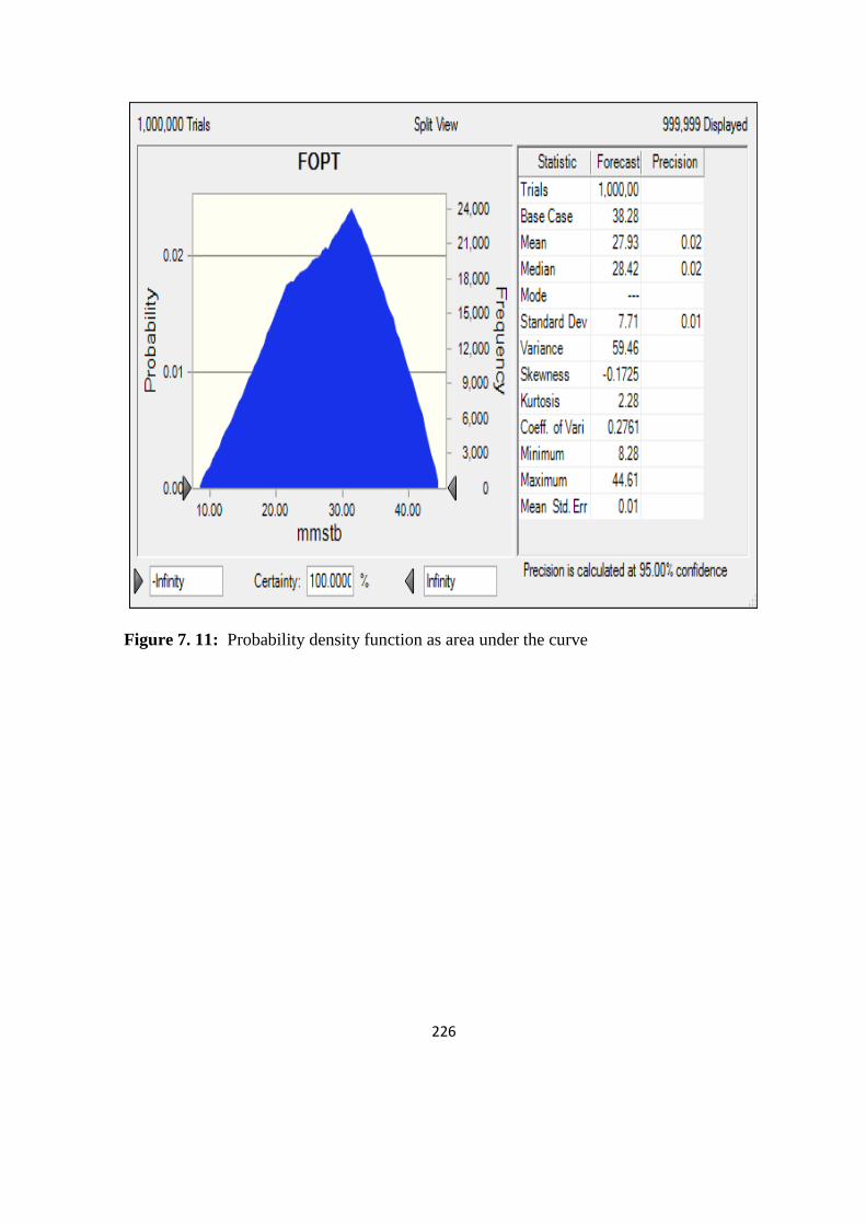
226
Figure 7. 11: Probability density function as area under the curve
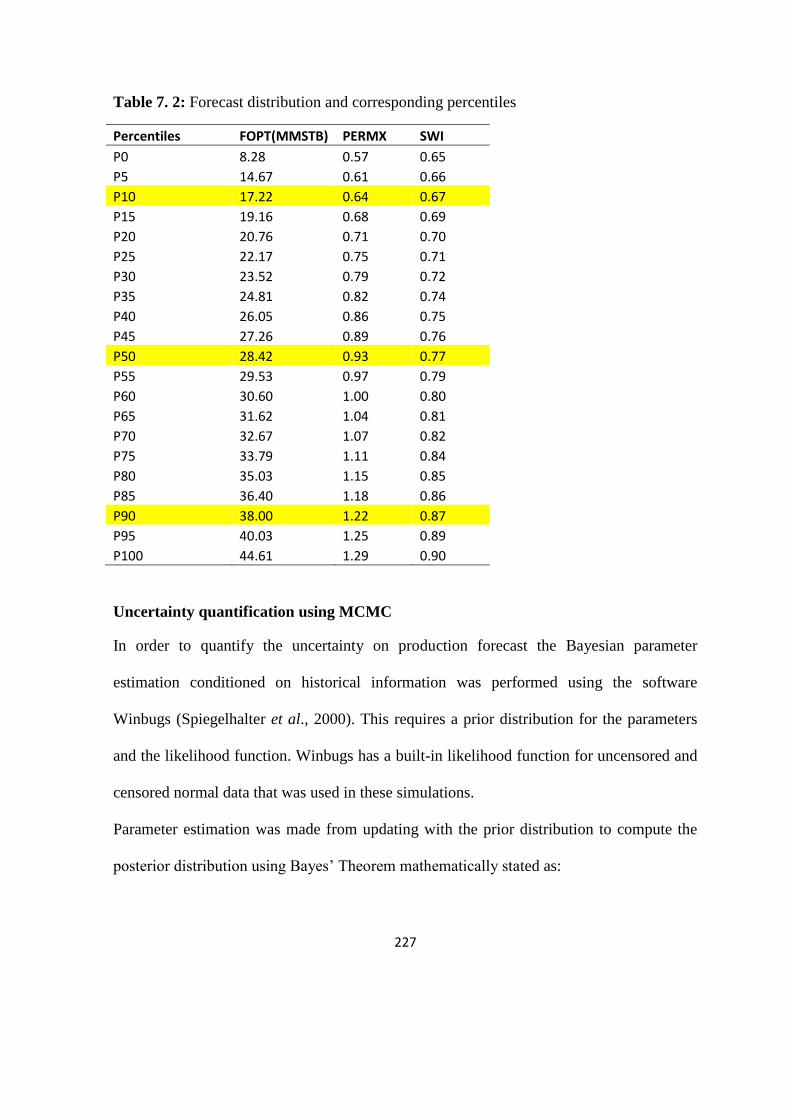
227
Table 7. 2: Forecast distribution and corresponding percentiles
Percentiles FOPT(MMSTB) PERMX SWI
P0 8.28 0.57 0.65
P5 14.67 0.61 0.66
P10 17.22 0.64 0.67
P15 19.16 0.68 0.69
P20 20.76 0.71 0.70
P25 22.17 0.75 0.71
P30 23.52 0.79 0.72
P35 24.81 0.82 0.74
P40 26.05 0.86 0.75
P45 27.26 0.89 0.76
P50 28.42 0.93 0.77
P55 29.53 0.97 0.79
P60 30.60 1.00 0.80
P65 31.62 1.04 0.81
P70 32.67 1.07 0.82
P75 33.79 1.11 0.84
P80 35.03 1.15 0.85
P85 36.40 1.18 0.86
P90 38.00 1.22 0.87
P95 40.03 1.25 0.89
P100 44.61 1.29 0.90
Uncertainty quantification using MCMC
In order to quantify the uncertainty on production forecast the Bayesian parameter
estimation conditioned on historical information was performed using the software
Winbugs (Spiegelhalter et al., 2000). This requires a prior distribution for the parameters
and the likelihood function. Winbugs has a built-in likelihood function for uncensored and
censored normal data that was used in these simulations.
Parameter estimation was made from updating with the prior distribution to compute the
posterior distribution using Bayes’ Theorem mathematically stated as:

228
p(θ D⁄ ) =f(D θ⁄ )ε(θ)
∫ f(D θ⁄ )ε(θ)dθ
The stochastic parameters β0, β1, β2 and τ are given proper prior distributions, while the
logical expression for σ allows the standard deviation to be estimated.
To check the convergence of MCMC simulations, multiple chains with divergent starting
points were run using derivative-free adaptive rejection sampling algorithm. Figure 7. 12
shows the trace plots for different parameters. The overlapping of the chains is an
indication that reasonable convergence has been achieved after 11000 iterations. To obtain
samples for posterior inference, Monte Carlo error was calculated for each parameter. A
total of additional 10000 simulations were required to obtain Monte Carlo error less than
5% of the sample standard deviation for all parameters.
Table 7. 3 shows the posterior summaries of the parameters of the regression coefficients
and the variance of the regression model. The posterior means and medians of the
coefficients of PERMX and SWI indicated that they are important variables. Moreover, it
was observed that the posterior means of β are slightly different from the ordinary least
square estimates [2.152, 52.58, - 17.31]T concluding that our prior was essentially a little
bit informative implementing minor on the model parameters.

229
Figure 7. 12: History plots showing two chains that are overlapped, an indication of
convergence
Table 7. 3: Posterior summaries of the indicator parameters included in the Bayesian
model
node mean sd MC error 2.5% 10% 50% 90% 97.5% start sample
beta0 2.152 1.020 0.0649 0.156 0.8411 2.164 3.43 4.098 12001 16000
beta1 52.580 1.041 0.0605 50.470 51.21 52.61 53.89 54.51 12001 16000
beta2 -17.310 0.993 0.0552 -19.36 -18.58 -17.29 -16.06 -15.4 12001 16000
Figure 7. 13 displays the posterior kernel density plots for model parameters βi. The
posterior distributions of the coefficients are normal for all the variables. The posterior
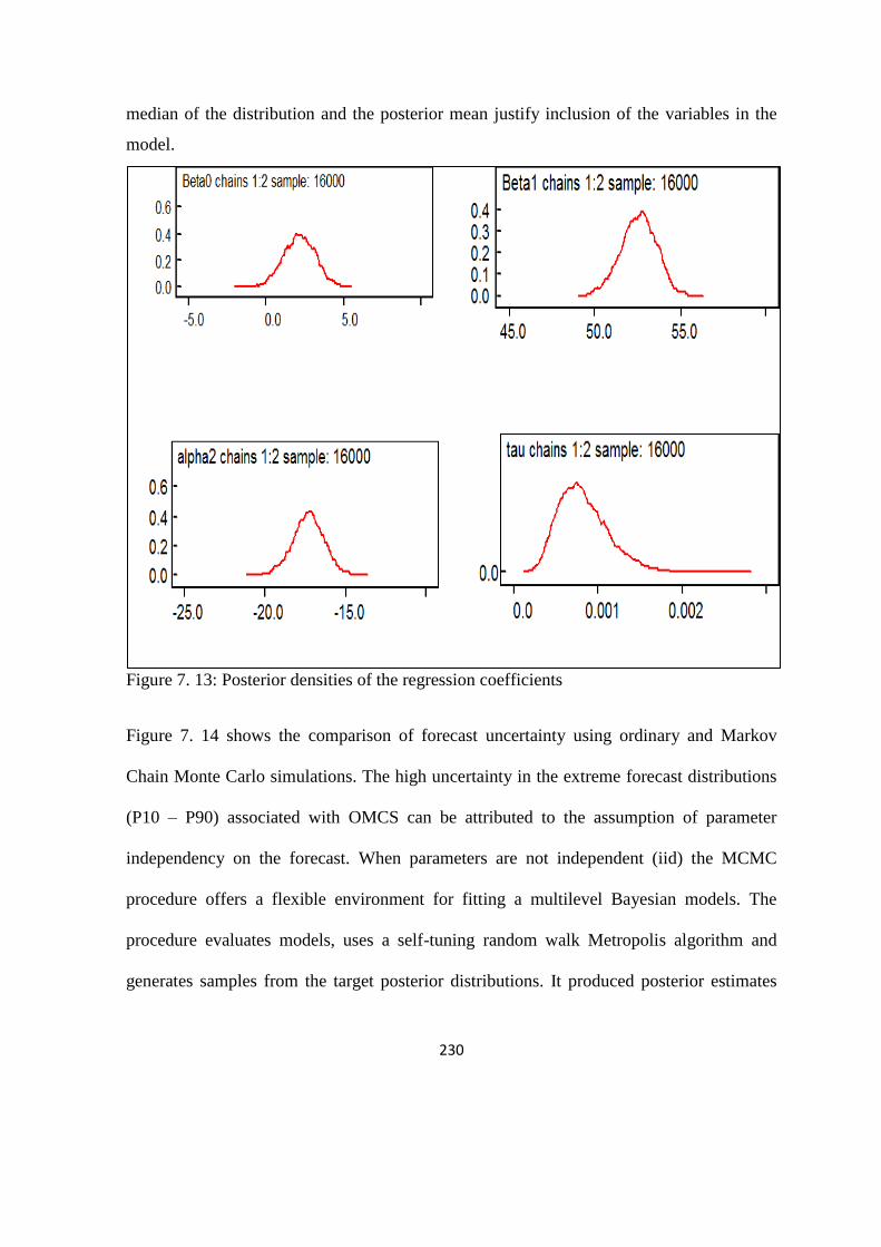
230
median of the distribution and the posterior mean justify inclusion of the variables in the
model.
Figure 7. 13: Posterior densities of the regression coefficients
Figure 7. 14 shows the comparison of forecast uncertainty using ordinary and Markov
Chain Monte Carlo simulations. The high uncertainty in the extreme forecast distributions
(P10 – P90) associated with OMCS can be attributed to the assumption of parameter
independency on the forecast. When parameters are not independent (iid) the MCMC
procedure offers a flexible environment for fitting a multilevel Bayesian models. The
procedure evaluates models, uses a self-tuning random walk Metropolis algorithm and
generates samples from the target posterior distributions. It produced posterior estimates

231
and convergence diagnostics. The parameter obtained using MCMC procedures are:
P2.5%, P10%, P50% P97.5% and P90%.
Figure 7. 14: Histogram showing comparison of forecast distribution using ordinary and
Markov Chain Monte Carlo simulations.
0
5
10
15
20
25
30
35
40
P10 P50 P90
Fore
cast
, MM
stb
Percentils
OMCS
MCMC

232
Chapter 8
8. Contribution to Knowledge
8.1 Major contributions
This research has contributed in the following ways:
1. An integrated approach combining use of site characterization, experiment design,
Monte Carlo simulation and oil/gas transport modeling is developed to address the
model and parameter uncertainties. The integrated framework presented can be
followed as a strategic procedure for assessing reservoir uncertainty.
2. Comparative study and what if analysis on implementation of different
experimental designs and responses surface algorithms used for variable screening
and response surface construction was presented. This is of high interests for
practitioners involved in predicting production curves or water cut and has potential
benefit for the community.
3. A simple framework for infill well placement and optimization is presented. The
method is simple, easy, straight forward and reproducible in other fields for
assessment of infill opportunity involving infill location, selection and placement.
4. Mathematical foundation that shows the differences and implications for wanton
use of Monte Carlo approximations for uncertainty quantification is presented with
example.

233
8.2 Published research articles
1. Arinkoola, A.O and Ogbe, D.O (2015): “Examination of experimental designs and
response surface methods for uncertainty analysis of production forecast: A Niger Delta
case study”, Journal of Petroleum Engineering, Vol. 2015, ID 714541,
http://dx.doi.org/10.1155/2015/714541.
2. Arinkoola, A.O., Haruna, M.O. and Ogbe, D.O (2015): “Quantifying uncertainty in
infill well placement using numerical simulation and experimental design: case study”,
Journal of petroleum exploration and production technology, ISSN 2190-0558, DOI
10.1007/s13202-015-0180-z, http://paperity.org/p/73385638.
3. Arinkoola, A.O., Aladeitan, M.Y and Ogbe, D.O (2015): “Integration of structural
uncertainty and experimental design for uncertainty quantification”, Journal of Petroleum
and Gas Engineering, Vol. 6 (7), pp. 74-89, DOI: 10.5897/JPGE2014.0209.
http://www.academicjournals.org/JPGE
4. Arinkoola, A.O., Duru, U.I. and Onuh, H.M (2015): “Development of proxy model for
production forecast using adaptive neuro-fuzzy inference system and experimental design”,
Int. J. Petroleum Engineering, Vol. 1, No. 3, pp.189-220.
http://www.inderscienceonline.com/doi/pdf/10.1504/IJPE.2015.071062

234
Chapter 9
9. Conclusion
This study addressed the issue of uncertainty identification, uncertainty quantification,
infill optimization and selection of appropriate experimental design methods for building
reservoir proxy model for reservoir management. These are problems areas being
confronted in many oil fields management and are important elements to consider in
planning the development of new concept for efficient recovery. In this research we built 3
stochastic models using structural map uncertainty. Majorly, well log data was used
following developed geological framework for properties distribution. We examined
various DoE methods, compared them and highlighted the implications of their arbitrary
usage for practical applications. We presented mathematical foundations for Monte Carlo
simulations and identified the implications of underlying assumptions in decision making.
In line with the set objectives, the summary of the derivatives of this study is provided as
follows:
9.1 Conclusions
1. Structural map uncertainty was successfully used as a basis for generating stochastic
models for uncertainty forecast of the volumes of hydrocarbons in place in a case study of
Niger Delta marginal field. A geological concept formulated proved adequate and allows
for multiple property integration. The approach adopted saves considerable time, permits

235
handling of relatively small static realizations, reproducible and very useful when only
limited data are available.
2. Optimization of infill location, selection and placement was successfully carried out
using numerical simulation of a full field study. Recoveries were evaluated in 4 different
fault blocks (A, B, C and D) and set of only vertical wells, only horizontal wells and
combination of vertical and horizontal wells were drilled. The number and type of infill
wells, horizontal well length, perforation intervals and inter-well spacing were considered
as uncertainty parameters. Two horizontal wells of 1000 meters lateral length each was
recommended for drilling and evaluation in the reservoir fault blocks B and D. The
methodology is useful as a practical guide where project delivery time is a serious issue of
concerns.
3. For uncertainty analysis, this study successfully examined three screening designs
(Placket-Burman, fractional factorial, and one variable at-a-time) and four response surface
methodologies (Box-Behnken, central composite, D-optimal, and full factorial) commonly
used for uncertainty analysis. In all screening methods, years of production forecast played
important role on associated number of “heavy-hitters.” Relative variation method (one
variable at-a-time) was identified with largest number of parameters and hence not
economical in application due to the attendant large number of simulation runs. Unlike
Placket-Burman, a low resolution fractional factorial in addition to main effects,
considered significance of factor interactions, required more simulation runs, but can
prevent exclusion of some factors with minimal main effect but significant interaction

236
effect. Nevertheless, the analysis performed in this study shows that there was no added
advantage using fractional factorial in lieu of Placket-Burman for screening.
It was agreed that, the selection of “best” model for uncertainty quantification must be
based on the reservoir management objectives. Box-Behnken method was adequate to
determine P10/P50/P90 and associated models within the analysis domain. On the other
hand, for future development strategies evaluation such as EOR, stimulation, and the needs
for acquiring additional information, full factorial and central composite designs are more
efficient predictors within acceptable margin of error. However, where full factorial 3-level
design is not practicable (when uncertainty number greater than 4), a 2-level factorial or
high resolution fractional factorial method was discovered to be adequate for the
construction of response surfaces for uncertainty quantification.
4. Response surface models developed using classical experimental designs in (3) above
are uneconomical and time consuming. The use of uniform design of experiment (UDoE)
and associated polynomial averaging method was found to be more advantageous in terms
of cost and time. Apart from accuracy, experimenter can decide on the number of
simulations based on available time and resources. The ANFIS-based model fitting
technique requires fewer parameters when compare with RSM based proxy-models and is
more accurate especially if there is occurrence of non-linearity between the dependent and
independent variables.
5. The application of Ordinary Monte Carlo analysis around a history match is not valid
since parameters are not independent and identically distributed. A full Bayesian treatment
is required, rather than a simple Monte Carlo approach.

237
Chapter 10
10. Future Works
10.1 Suggestions for Future Work
Several areas of applications of experimental design, response surface methodologies,
Fuzzy logic and optimal control theory are suggested as potential areas for future research.
1. Application of the experimental design/response surface methodology for history
matching and prediction of multi-response reservoir performance. It would be interesting
to see if a response surface can predict many flow responses accurately.
2. RSM-based proxy models are purely statistical and have no consideration of the physics
underlying the process, a proxy that can be calibrated and one that honors physics would
be very useful for the purpose of optimization of petroleum reservoirs. For risk analysis, a
method that integrates history matching and risk workflow is desirable.
3. The use of experimental design to investigate well interference and optimum number of
wells within the reservoir.
4. Investigate adaptive control theory, Fuzzy logic and optimal control methodologies for
history matching, uncertainty analysis and well placement optimization

238
5. Reservoir performance predictions and forecast using knowledge discovery in databases
(KDD). This will involve taking the advantages of the advancements in hardware and
software to analyze large amounts of production data using data science techniques.
6. Investigate the economic impact of decisions obtained from short-term production
optimizations on long-term oil recovery.

239
Nomenclature
ANFIS Adaptive Neuro-Fuzzy Inference System
M Thousand
MM Million
STB Stock-Tank-Barrel
MULTFLT Fault transmissibility multiplier
PV Pore Volume
FVF Oil Formation Volume Factor
F Field
WCT Water cut
OPT Total oil production
WPT Total water production
GOR Gas-oil ratio
PERMX Horizontal permeability
PERMZ Vertical permeability
WBT Water breakthrough time
SWI Initial water saturation
PORO Porosity
OVISC
P10
P50
P90
mD
PV
STOIIP
Oil viscosity
10 Ppercentile
50 percentile
90 percentile
Millidarcy
Pore volume
Stock tank oil initial in place

240
Symbol
β formation volume factor
σ2 variance
ϵ subset
γ ( ) variogram function
λ kriging weight
φ porosity
σ standard deviation
C ( ) covariance function
J productivity index
Subscripts
a aquifer
r reservoir
t total
min minimum
max maximum
i coordinate, initial
j coordinate
E error
o, w, g Oil, water, gas
c criticalwater
Superscripts
D dimension
T transpose

241
Bibliography
Adams, S. J. (2005): “Quantifying Petrophysical Uncertainties” SPE 93125 paper
presented at the Asia Pacific Oil & Gas Conference and Exhibition held in
Jakarta, Indonesia, 5 – 7 April
Ahmed, T. and Mckinney, D.P. (2005): Advanced Reservoir Engineering, 1st Edition,
Elsevier, Gulf Professional Publishing, New York
Aigbodion, V.S., Hassan, S. B, Dauda, E. T and Mohammed, R. A (2010): The
Development of Mathematical Model for the Prediction of Ageing Behavior for Al-
Cu-Mg/Bagasse Particulate Composite. J. of Minerals & Materials
Characteristics &Engineering, (9): 907-917
Al-Shamma, B.R. and Teigland, R., (2006): History Matching of The Valhall Field Using a
Global Optimization Method and Uncertainty Assessment, SPE 100946, presented
at SPE Annual Technical Conference and Exhibition (Sept., 2006).
Alabert, F., (1987): The Practice of Fast Conditional Simulation Through the LU
Decomposition of the Covariance Matrix; Math Geology, Vol. 19, No. 5, pp. 369-
386, 1987
Alhuthali, A.H., Oyerinde, D. and Datta-Gupta, A., (2006): Optimal Waterflood
Management Using Rate Control, SPE 102478, presented at SPE Annual
Technical Conference and Exhibition (Sept., 2006).
Allen, T. T., Bernshteyn, M.A., and Kabiri- Bamoradian, K. (2003): Constructing
metamodels for computer experiments. Journal of Quality Technology, 35:264-
274

242
Almeida Netto, Schiozer D.J., Ligero, E.L., Maschio, C. (2003): History matching Using
Uncertainty Analysis. SPE International Conference, Society of Petroleum
Engineers. Calgary, Alberta, Canada
Amudo C., Graf T., Haris N.R., Dandecar R., Ben Amor F. and May R.S (2008): ”
Experimental Design and Response Surface Models as a Basis for Stochastic
History Match- A Niger Delta Experience” IPTC 12665 presented at the
2008 International Petroleum Technology Conference, Kuala Lumpa, Malaysia,
Dec. 3-5
Apaydin, O.G., Iwere, F.O., Luneau, B., and Ma, Y (2005): “Critical Parameters in Static
and Dynamic Modeling of Tight Fluvial Sandstones,” SPE 95910 presented at
the SPE Annual Technical Conference and Exhibition, Dallas, Texas, USA,
9-12 October,
2005
Artem ratchkovski, david O. Ogbe and Akanni S. Lawal (1999):”Application of
Geostatistics and Conventional Methods to Derive Hydaulic Flow Units for
Improved Reservoir description: A Case of Edicott Field, Alaska,” paper SPE
54587 presented at 1999 SPE Western Regional Meeting, Anchorage,
Alaska, May 26-23
Ates, H., Bahar, A., El-Abd, S., Charfeddine, M., Kelkar, M. and Datta- Gupta, A (2005):
Ranking and Upscaling of Geostatistical Reservoir Models by Use of Streamline
Simulation: A field Case Study, paper SPE 81497, SPE Reservoir Evaluation and
Engineering, Feb., 2005.
Azuka, C. A, Ali, S. S, and Tara La Force (2009): Uncertainty Evaluation in Field

243
Development and Export Planning. Paper SPE 121993 presented at the SPE
EUROPEC/EAGE Annual conference and exhibition held at Amsterdam, The
Netherlands, 8-11 June, 2009
Ballin, P.R., Aziz, K., Journel, A.G (1993): ”Quantifying the Impact of Geological
Uncertainty on Reservoir Performing Forecasts,” paper SPE 25238 presented at
the 12th SPE Symposium on Reservoir Simulation, New Orleans, USA, 28 Feb –
3 March 1993.
Ballin, P.R., Clifford, P.J. and Christie, M.A., Cupiagua (2001): A Complex Full-Field
Fractured Reservoir Study Using Compositional Upscaling, paper SPE 66376,
presented at SPE Reservoir Simulation Symposium, Houston, Feb., 2001.
Bi Z, Oliver D S and Reynolds A C (2000): Conditioning 3D Stochastic Channels to
Pressure Data. SPE Jounal 5 474 484
Box, G.E.P., Hunter, W. G., and Hunter, J.S. (2005): Statistics for experimenters: Design,
Innovation, and Discovery, 2nd Edition, John Wiley & Sons, New York
Bustamante, D.S., Keller, D.R. and Monson, G.D. (2005): Understanding Reservoir
Performance and Uncertainty using a Multiple History Matching Process, paper
SPE 95401, presented at Annual Technical Conference and Exhibition
(Oct., 2005).
Carlson, M.R.: Practical Reservoir Simulation, PennWell, Tulsa, (2003): Chambers, R.L.,
Yarus, J.M. and Hird, K.B. (2000): “Petroleum Geostatistics for
Nongeostatisticians – Part 1,” The Leading Edge (May 2000) 474-479.
Castellini, A., Yeten, B., Singh, U., Vahedi, A., Sawiris, R (2006): "History Matching and
Uncertainty Quantification Assisted by Global Optimization Techniques," 10th

244
European Conference on the Mathematics of Oil Recovery — Amsterdam,
The Netherlands 4 – 7 September 2006
Castellini, A., Chawathe, A., Larue, D., Landa, J.L., Jian, F.X., and Toldi, J.L (2003):
“What is Relevant to Flow? A Comparative Study Using a Shallow Marine
Reservoir,” SPE 79669 presented at the SPE Reservoir Simulation
Symposium, Houston, Texas, USA, 3-5 February, 2003
Chavent G, Dupuy M and Lemonnier P (1975): History matching by use of optimal theory,
SPE 4627, SPE Journal, 15(1) 74–86
Coates, G. R and Dumanoir, J. L (1974): “A New Approach To Improved Log – Derived
Permeability.”: The Log Analyst, Pp17. (January-February 1974).
Coates, G. R And Denoo, S. (1981): “The Producibility Answer Product” The Technical
Review, Schlumberger Hauston (June 1981) 29 No. 2 P55-63
Corre, B., Thore, deFeraudy, V., Vincent, G. (2000): “Integrated Uncertainty Assessment
for Project Evaluation and Risk Analysis,” paper SPE 65205, presented at SPE
European Petroleum Conference, Paris, France, 24-25 Oct 2000.
Cotento, F.M, Godi A, Nicota G, and Pizzo A; “ A Risk Analysis Approach: From
Subsurface to Siurface” IPTC 10493 presented at the International Petroleum
Technology Conference, Doha, Qatar, 21-23 November, 2005
Cullick, A. S., Johnson D., and Shi G., (2006):”Improved and More-Rapid History
Matching with a Nonlinear Proxy and Global Optimization”. Paper SPE 101993
presented at the SPE Annual Technical Conference and Exhibition, San
Antonio, Texas, 24-27 Sept
Da Cruz, P.S., Horne, R.N., Deutsch, C.V. (2004): “The Quality Map: A Tool for

245
Reservoir Uncertainty Quantification and Decision Making,” SPEREE (Feb
2004), 6
Dake, L.P. (1978): Fundamentals of Reservoir Engineering, Elsevier Scientific Publishing
Company, Amsterdam (1978).
David O. Ogbe, Fabian O. Iwere, Ernie Gomez and Ekeng Henshaw (2009): “Conceptual
Model for Fast Tracking Decision Making in the Reservoir Management” SPE
121392 Paper presented at the SPE Western Regional Meeting held in San Jose,
Califonia, USA, 24- 26 Mach
Dejean, J.P. and Blanc, G. (1999): “Managing Uncertainties on Production Predictions
Using Integrated Statistical Methods,” paper SPE 56696 presented at the 1999
SPE Annual Technical Conference and Exhibition, Houston, 3–6 October.
De Waal, J. A. Smits, R.M.M, de Graaf, J.D, Schipper, B. A. (1991): Measurement and
Evaluation of Resistivity- index Curves. The Log Analyst, September- October
1991, Pp583-595
Deutsch C. V, Srinivasan S. and Mo Y (1996): “Geostatistical Reservoir Modeling
Accounting for Precision and Scale of Seismic Data” Paper SPE 36497
presented at the 1996 SPE Annual Technical Conference and Exhibition held in
Denver, Colorado, U S A, 6-9 October 1996.
Dong Y and Oliver D S (2005): Quantitative Use of time-lapse Seismic Data for Reservoir
Description, SPE 84571, SPEJ, 10 91-99.
Dong Y and Oliver D S (2008): Reservoir Simulation Model Updates via Automatic
History Matching With Integration of Seismic Impedance Change and
Production Data, SPE 12550, International Petroleum Technology Conference,
Kuala Lumpur, Malaysia, December 3-5

246
Dunlop, K.N.B., Vossepoel, F.C., Xu, R., Sarma, P., Alhutali, A.H., Reynolds, A.C.
(2010): Results of the Brugge benchmark study for flooding optimization and
history matching. SPE Reserv. Evalu. Eng. 13(3), 391–405 (2010)
Durlofsky, L.J. (2003): Upscaling of Geocellular Models for Reservoir Simulation: A
Review of Recent Progress, paper presented at 7th International Forum on
Reservoir Simulation, Germany (June 2003).
Dykstra, H. and Parsons, R. L. (1950): “The Prediction of Oil Recovery in Waterflood.”
Seconday Recovey of Oil in the United States, 2nd ed. American Petroleum
Institute (API), 1950, pp. 160-174.
Egbogah, E. O. (1994): “EOR Target Oil and Techniques of its Estimation,” J. Petr. Sc.
and Eng., 10 (334)
Ekwere Peters (210): Advanced Petrophysics, African University of Science and
Technology, Abuja, Course material for PE223, 2010
Eiben, A.E., Smith, J.E. (2003): "Introduction to Evolutionary Computing," Springer,
Berlin (2003)
Evensen G (2003): The Ensemble Kalman Filer: theoretical formulation and practical
implementation, Ocean Dynamics, 53 343–367.
Evensen, G. (2007): "Data Assimilation, The Ensemble Kalman Filter," Springer, Berlin
(2007)
Evensen, G., Hove, J., Meisingset, H.C., Reiso, E., Seim, K.S., Espelid, O (2007): "Using
the EnKF for Assisted History Matching of a North Sea Reservoir Model,"
paper 106184 presented at the 2007 Reservoir Simulation Symposium, The
Woodlands, USA, 2007

247
Fasanino G, Molinard J E, de Marsily G and Pelcé V (1986): Inverse Modeling in Gas
Reservoirs, SPE 15592, 61st SPE Annual Technical Conference and Exhibition,
New Orleans, Texas, October 5-8.
Fatemeh Moeinikia and Nassar Alizadeh (2012): Experimental Design in Reservoir
Simulation: An Integrated Solution for Uncertainty analysis, a case study. J.
Petrol. Explor. Prod. Technol., 2, 75-85
Femi V. Akinwumi, Elias C. Arochukwu, and Abiola S. Abdul-Kareem,” Managing
Uncertainties in Hydrocarbon-in-place Volumes in a Northern Depobelt Field,
Niger Delta, Nigeri”a . SPE 88880 Paper presented at the 28th Annual SPE International
Technical Conference and Exhibition in Abuja, Nigeria, August 2-4, 2004.
Friedmann, F. Chawathe, A. Larue D.K (2003): Assessing Uncertainty in Channelized
Reservoirs Using Experimental Designs; SPE 85117, SPE Reservoir Evaluation &
Engineering August 2003
Fuller, S.M., Sarem, A.M., and Gould, T.L (1992): Screening Waterfloods for Infill
Drilling Opportunities, paper SPE 22333 presented at the SPE International
Meeting on Petroleum Engineering held in Beijing, China, 24-27 March,
1992.
Gen, M., Cheng, R. (2000): "Genetic Algorithms & Engineering Optimization," John
Wiley & Sons, Inc., New York (2000)
Gilks, W.R., Richardson, S. and D.J. Spiegelhalter. (1996). Markov chain Monte Carlo
Methods in practice, Chapman & Hall
Gu Y, Oliver D S (2004): History Matching of the PUNQ-S3 Reservoir Model Using the
Ensemble Kalman Filter, SPE 89942, SPE Annual Technical Conference and
Exhibition, Houston, USA, September 26-29.

248
Guohua G, Gaoming L and Reynolds A C (2004): A stochastic optimization algorithm for
automatic history matching, SPE 90065, SPE Annual Technical Conference and
Exhibition, Houston, Texas, September 26-29.
Hook, J. R (1983): The Precision of Core Analysis Data and Some Implications for
Reservoir Evaluation. SPWLA Twenty- Fourth Annual Logging Symposium June 27-
30, 1983. Paper Y.
Hudson, J.W., Jochen, J.E., and Jochen, V.A (2000): Practical Technique to Identify Infill
Potential in Low- permeability Gas Reservoirs Applied to the Milk River
Formation in Canada, paper SPE 59779 presented at the 2000 SPE/CERI Gas
Symposium, Calgary, 3- 5 April.
Hui, M., Zhou, D., Wen, X. and Durlofsky, L.J (2004): Development and Application of a
New Technique for Upscaling Miscible Processes, paper SPE 89435, presented at
SPE/DOE Symposium on Improved Oil Recovery, Tulsa (April 2004).
Idrobo, E.A., Choudhary, M., and Datta-Gupta, A (2000): “Swept Volume Calculations
and Ranking of Geostatistical Reservoir Models Using Streamline Simulation,”
paper SPE 62557 presented at the 2000 SPE/AAPG Western Regional Meeting,
Long Beach, California, 19–23 June.
Jacquard P and Jain C (1965): Permeability distribution from field pressure data, Soc. Pet.
Eng. Journal, 281-294.
Jafarpour B., and McLaughlin D.B. (2007): History matching with an Ensemble Kalman
filter and discreate cosine parameterization. paper SPE 108761 presented at SPE
Annual Technical Conference and Exhibition, Anaheim, USA, 11-14
November.
Journel, A.G. and Alabert, F (1990): New Method for Reservoir Mapping; Journal of

249
Petroleum Technology, pp. 212-218, February 1990. June.doi:
10.2118/113498-MS
Kalla, S. and White, C. D. (2007): Efficient Design of Reservoir Simulation Studies for
Development and Optimization, SPE-95456-PA, Res Eval & Eng 10 (6); 629-637.
Doi: 10.2118/95456-PA
Kelkar, M, Godofredo, P (2002): “Applied Geostatistics for Reservoir Characterization,”
published by SPE, 2002.
G. Kuczera & E. Parent (1998). Monte Carlo assessment of parameter inference in
Catchments models: The Metropolis algorithm. Journal of Hydrology, 211, pp.69 –
85
Lambers, J. and Gerritsen, M (2005): An Integration of Multilevel Local-Global Upscaling
with Grid Adaptivity, paper SPE 97250, presented at SPE Annual Technical
Conference and Exhibition, Dallas (Oct. 2005).
Lamy, P., Swaby, P.A., Rowbotham, P.S., Dubrule, O. and Haas, A. (1998): From Seismic
to Reservoir Properties with Geostatistical Inversion, SPE 57476, Annual
Technical Conference and Exhibition (1998)
Li R, Reynolds A C and Oliver D S (2003): History matching of three-phase flow
production data, SPE Journal, 8(4) 328–340, 2003.
Li, Y. and Johns, R.T (2005): Rapid Flash Calculations for Compositional Modeling, SPE
95732, Annual Technical Conference and Exhibition (Oct., 2005).
Little, A.J., Jutila, H.A., Fincham, A (2006): "History Matching With Production
Uncertainties Eases Transition Into Prediction," paper SPE100206 accepted for
publication at the SPE Europec/EAGE Annual Conference and Exhibition
held in Vienna, Austria, 12-15 June 2006

250
Linhua Guan, Yuqi Du, Zhiming Wang (2005): Infill Drilling-lessons Learnt In the Past 20
Years, 18th World Petroleum Congress, September 25 - 29, 2005, Johannesburg,
South Africa Copyrigh t2005. World Petroleum Congress
Manceau, E., Mezghani, M., Mezghani, I. Z., Rogero, F (2001):”Combination of
Experimental Design and Joint Modeling Methods for Quantifying the Risk
Associated with Deterministic and Stochastic Uncertainties – An Integrated
Test Study; SPE 71620. SPE Annual Technical Conference and Exhibition, New
Orleans, Louisiana, 30 September – 3 October 2001.
Mattax C. C. and Dalton R L (1991): Reservoir simulation, SPE 20399, Journal of
Petroleum Technology, 42 692-695.
Mclennan, J and Deutsch, C (2005): Ranking Geostatistical Realizations by Measures of
Connectivity; Society of Petroleum Engineers (SPE), Paper 98168, 2005.
Meisingset, K.K. (1999): “Uncertainties in Reservoir Fluid Description for Reservoir
Modeling,” SPEREE Oct 1999, 2 (5).
Mohaghegh, S.D., Hafez Hafez, Razi Gaskari and Masoud Haajizadeh (2006): Uncertainty
Analysis of a giant Oil Field in the Middle East Using Surrogate Reservoir Model,
SPE 101474, presented at SPE International Petroleum Exhibition and (Nov.,
2006)
Mohaghegh, S (2000): Virtual-Intelligence Applications in Petroleum Engineering: Part
1—Artificial Neural Networks. Journal of Petroleum Technology [S.I.], v. 52, n.
9, p. 8, September
Montgomery, Douglas C (2005): Design and Analysis of Experiments: Response surface
method and designs. New Jersey: John Wiley and Sons, Inc.

251
Morris, M.D. (2000): Three techno metrics experimental design classics. Techno metrics,
42(1): 26-27
Mu’azu. K., Mohammed-Dabo, I.A and Waziri, S.M (2012): “Development of
Mathematical Model for the Prediction of Essential Oil Extraction from
Eucalyptus Citriodora Leave” J. Basic. Appl. Sci. Res., 2(3)2298-2306
Ogbalor Cyril and Anthony Peacock (2010): “Using Experimental Design with Reservoir
simulation to Manage Subsurface Uncertainties-A Niger Delta Case Study,” paper
SPE 140613 presented at the 34th Annual SPE international Conference and
Exhibition, Tinapa-Calabar, Nigeria, July 31-August 7, 2010
Ofoh, E.P (1992): Geological Heterogeneity in the Niger Delta: A Case for Additional
Recovery through a Combined Effort of Geologically Targeted infill Drilling,
Stimulation, and Gas-Lift Installation, paper SPE 24745 presented at the 67th,
1992
Olatunji, S.O, Selamat, A., Abdul Raheem, A. and Omatu, S (2011): “Modeling the
Correlations of Crude Oil Properties based on Sensitivity Based Linear Learning
Method”. Engineering Applications of Artificial Intelligence, 24: 686-696
Olea, R.A (1991): “Geostatistical Glossary and Multilingual Dictionary,” Oxford
University Press, 1991.
Oliver D S, Chen Yan (2010): Recent progress in history matching, a review, journal of
ComputGeosci, © Springer Science+Business Media B.V.2010
Pathak R, Ogbe, D. O and Jensen,J. L. (2000): Application of Geostatistical and Fluid
Flow Simulations to Evaluate Options for Well Placement. Paper SPE 62554
presented at the 2000 SPE/AAPG Western Regional Meeting held in Long Beach,
California, 19–23 June 2000.

252
Peaceman, D.W (2003): A New Method for Calculating Well Indexes for Multiple
Wellblocks with Arbitrary Rates in Numerical Reservoir Simulation, SPE
79687, SPE Reservoir Simulation Symposium (Feb., 2003).
Peak W.T., Abadah M. and Skander L.:”Uncertainty Assessment Using Experimental
Design: Minagish Oolite Reservoir,” paper SPE 91820 presented at the 2005
SPE Reservoir Simulation Symposium, Houston, Texas, Jan. 31-Feb. 2
Peng, C.H., & Gupta, R (2003): Experimental Design in Deterministic Modeling:
Assessing Significant Uncertainties; SPE 80537. SPE Asia Pacific Oil and Gas
Conference, Jakarta, Indonesia, 9-11 September 2003.
Peters, L., Arts, R.J., Brouwer, G.K., Geel, C.R., Cullick, S., Lorentzen, R.J., Chen, Y.,
Dunlop, K.N.B., Vossepoel, F.C., Xu, R., Sarma, P., Alhutali, A.H.,
Reynolds, A.C. (2010): Results of the Brugge benchmark study for
flooding optimization and history matching. SPE Reserv. Evalu. Eng. 13(3),
391–405 (2010)
Phan, V. and Horne, R.N (1999): Determining Depth-Dependent Reservoir Properties
using Integrated Data Analysis, paper SPE 56423, presented at Annual Technical
Conference and Exhibition (Oct., 1999).
Ph. Theys (1997): “accuracy- Essential Information for a Log measurement” SPWLA 38th
Annual Logging Symposium, June 15-18, 1997 Paper V
Risso, F.V.A, Risso, V.F, and Schiozer, D.J. (2007):” Risk Assessment of Oil Field Using
Proxy Models: A Caser Study” paper 2007-138 presented at the Petroleum
Society’s 8th Canadian International Petroleum Conference, Calgary, Alberta,
Canada, June 12-14

253
Roger Jang, J. S. (1993): ‘’ANFIS: Adaptive-Network-Based Fuzzy Inference System’’
Transactions on Systems, Man, and Cybernetics, Vol. 23, No. 3, pp665-685, 1993
Roggero, F., Hu, L.Y (1998): "Gradual Deformation of Continuous Geostatisticals Model
for History Matching," paper SPE 49004 presented at the SPE 1998 Annual
Technical Conference and Exhibition, New Orleans, USA.
Ruijian L, Reynolds A C, Oliver D S (2003): History Matching of Three-Phase Flow
Production Data, SPE 87336, SPE Journal, 4 328-340.
Sablok, R. and Aziz, K (2005): Upscaling and Discretization Errors in Reservoir
Simulation, paper SPE 93372, presented at SPE Reservoir Simulation
Symposium, Houston (Feb. 2005).
Salam, K.K, Araromi, D.O, Ikiensikimama, S.S. (2011): “Neuro-Fuzzy Modeling for the
Prediction of below-Bubble-Point Viscosity. Petroleum Science and Technology.
2011;29(17):1741-1752.
Sandsdalen, L., Barbieri, M., Tyler, K., and Aasen, J.O (1996) : "Applied Uncertainty
Analysis Using Stochastic Modeling ", paper SPE 35533 presented at the
European 3-D Reservoir Modeling Conference, Stavanger (norway), 16-17
April 1996.
Sampaio, T. P, Ferreira Filho, V. J. M, de Sa Neto, A. (2009): SPE 122148 presented at
The 2009 SPE Latin American and Caribbean Petroleum Engineering Conference
held in Cartagena, Colombia, 31May–3 June.
Schaaf, T., Coureaud, B., and Labat, N. (2008): Using Experimental Designs, Assisted
History Matching Tools and Bayesian Framework to get Probabilistic
Production Production Forecast. Paper SPE 113498 presented at the
Europe/EAGE Conference and Exhibition, Rome, 9-12

254
Schiozer, D J, Sousa S H G (1997): Use of External Parallelization to Improve History
Matching, SPE 39062, Latin American and Caribbean Petroleum Engineering
Conference, 1997, Rio de Janeiro, Brazil, August 30 - September 3
Schiozer, D.J., Ligero, E.L., Suslick, S.B.;Costa, A.P.A., Santos, J.A.M.(2004): Use of
Representative Models in the Integration of Risk Analysis and Production Strategy
Definition, JPSE, n1- 2, v.44, pp.131-141, 2004
Schulze-Riegert, R., Haase, O., Nekrassov, A. (2003): "Combined Global and Local
Optimization Techniques Applied to History Matching," paper SPE 79668 prepared
for presentation at the SPE Reservoir Simulation Symposium held in Houston,
Texas, U.S.A., 3–5 February 2003
Schulze-Riegert, R., Krosche, M., Fahimuddin, A., Ghedan, S (2007): "Multi-Objective
Optimization with Application to Model Validation and Uncertainty
Quantification," paper SPE 105313 presented at the 15th SPE Middle East Oil &
Gas Show and Conference, Kingdom of Bahrain, 11–14 March 2007.
Selberg, S., Schulze-Riegert, R., Stekolschikov, K (2007): "Event Targeting Model
Calibration Used for History Matching Large Simulation Cases," paper 106044
was prepared for presentation at the 2007 SPE Reservoir Simulation
Symposium held in Houston, Texas, U.S.A., 26–28 February 2007
Smith, A. E M. and Roberts, G. O. (1993) Bayesian computation via the Gibbs sampler
And related Markov chain Monte Carlo methods. J R. Statist. Soc. B, 55, 3-23.
Sprunt, E. S, Hensel, W. M., York, C. E, Honarpour, M. M (1988).: Compilation of
Electrical Resistivity Measurements Performed by Twenty- Five Laboratories.
The Log Analyst, January- February 1988, P.13-39
Steagall, D.E. and Schiozer, D.J (2001): Uncertainty Analysis in Reservoir Production

255
Forecasts During Appraisal and Pilot Production Phases; paper SPE 66399
presented at the SPE Reservoir Simulation Symposium, Houston, TX, 11-14
February, 200
Stern, D (2005): “Practical Aspects of Scaleup of Simulation Models,” SPE 89032, SPE
JPT (September, 2005)
Subbey, S., Christie, M. and Sambridge, M. (2003): A Strategy for Rapid Quantification of
Uncertainty in Reservoir Performance Prediction, paper SPE 79678, presented at
SPE reservoir simulation symposium (Feb., 2003).
Thakur, G.C. and Satter, A. (1998): Integrated Waterflood Asset Management, PennWell,
1998.
Timur, A (1968): “An Integration Of Permeability, Porosity and Residual Saturation
Relationship For Sandstone Reservoirs”.: The Log Analyst, Vol. 9 No. 4 Pp. 8 (
July- August 1968).
Tyler, K., Sandsdalen, L., Maeland, J.O., Aasen, J.O., Siring, E., and Barbieri, M. (1996) :
"Integrated Stochastic Modeling in Reservoir Evaluation for Project Evaluation and
Risk Assessment", paper SPE 36706 resented at the 1996 SPE Annual Technical
Conference and Exhibition, Denver, 6-9 October
Vega, L., Rojas, D. and Datta-Gupta, A (2003): Scalability of the Deterministic and
Bayesian Approaches to Production Data Integration into Field-Scale
Reservoir Models, paper SPE 79666, presented at SPE Reservoir Simulation
Symposium (Feb., 2003).
Vanegas, J.W, Cunha, J.C, and Cunha, L. B. (2006): “Uncertainty Assessment of
production Performance for a Heavy Oil Offshore Field by using the
Experimental Design Technique”, paper 2006-125 presented at the Petroleum

256
society’s 7th Canadian International Petroleum Conference, Calgary,
Alberta, Canada, June 13-15, 2006.
Verbruggen, R., Pannett, S., Stone, G. (2002): “Understanding Reserves Uncertainties in a
Mature Field by Reservoir Modeling,” paper SPE 77896, presented at the SPE Asia
Pacific Oil and Gas Conference and Exhibition, Melbourne, Australia, 8-10 Oct
2002.
Vincent, G., Corre, B., Thore, P (1999): “Managing Structural Uncertainty in a Mature
Field for Optimal Well Placement,” SPEREE August 1999, 2(4).
Voneiff, G.W. and Cipolla, C. (1996): A New Approach to Large-Scale Infill Evaluations
Applied to the Ozona (Canyon) Gas Field, paper SPE 35203 presented at the 1996
SPE Permian Oil and Gas Recovery Conference, Midland, Texas, 7-29 March.
Walstrom, J.E., Mueller, T.D., McFarlane, R. C. (1967): “Evaluating Uncertainty in
Engineering Calculations,” Journal of Petroleum Technology, Dec 1967, p 1595
Wen, X.H., Chen, W. (2005): "Real-Time Reservoir Model Updating Using Kalman
Filter," paper 92991 presented at the 2005 Reservoir Simulation Symposium, The
Woodlands, USA, 2005
Williams, G.J.J., Mansfield, M., MacDonald, D., Bush, M. D. (2004): "Top-Down
Reservoir Modeling," paper SPE89974 presented at the ATCE 2004, Houston,
Texas, 26-29. Sep. 2004
Yeten B., Castellini, A., Guyagular, B., and Chen, W. H. (2005): “A comparison Study on
Experimental Design and Response Surface Methodologies”. Paper SPE 93347
presented at the SPE Reservoir Simulation Symposium, Houston, Texas, USA,
Jan. 31- Feb. 2

257
Zhang, D. (2002): Stochastic Methods for Flow in porous Media: Coping with
Uncertainties.
San Diego, California: Academic Press.

258
APPENDIX A
Correlations used for the Synthetic log Estimations
1. Volume of shale estimation
𝑉𝑠ℎ 𝑆𝑡𝑒𝑖𝑏𝑒𝑟 (1970) =𝐺𝑅 𝐼𝑛𝑑𝑒𝑥
1.5 − 𝐺𝑅 𝐼𝑛𝑑𝑒𝑥 𝐴1
𝐺𝑅 𝐼𝑛𝑑𝑒𝑥 =[𝐺𝑅𝑙𝑜𝑔 − 𝐺𝑅𝑚𝑖𝑛]
[𝐺𝑅𝑚𝑎𝑥 − 𝐺𝑅𝑚𝑖𝑛] 𝐴2
2. Total and effective porosity estimation
Total porosity was obtained from the Formation Density (FDC) logs. A grain density of
2.65 g/cc, which is typical of the Niger Delta, and densities of 1.00 g/cc for water, 0.6 g/cc
for oil and 0.20 g/cc for gas can be used.
𝑃𝐻𝐼𝑇 = 0.67 ∗ 𝐷𝑇 − 𝐷𝑇𝑚𝑎𝑥
𝐷𝑇 𝐴3
𝑃𝐻𝐼𝑇 =𝑅𝐻𝑂𝑚𝑎𝑡𝑟𝑖𝑥 − 𝑅𝐻𝑂𝑙𝑜𝑔
𝑅𝐻𝑂𝑚𝑎𝑡𝑟𝑖𝑥 − 𝑅𝐻𝑂𝑓𝑖𝑙𝑡𝑟𝑎𝑡𝑒 𝐴4
𝑃𝐻𝐼𝐸 = 𝑃𝐻𝐼𝑇 ∗ (1 − 𝑉𝑠ℎ) 𝐴5
3. Water saturation
Indonesian correlation for water saturation

259
This assumed m = 2, a = 1 and n = 2
𝑆𝑤 = √(1
𝑅𝑡−
𝑉𝑠ℎ
𝑅𝑠ℎ) ∗
𝑅𝑤(1 − 𝑉𝑠ℎ)2
∅2 𝐴6
GRIndex = linear relationship between Gamma ray log and Volume of shale
GRmin = Gamma ray log reading in 100% clean zone in API unit
GRmax = Gamma ray log reading in 100% shale zone in API units
PHIT = Total porosity
DTma = interval travel transit time in matrix (sandstone) 55.5μft/s
DT = transit time log
RHOM = Density of matrix (2.60 - 2.65 g/cc)
RHOB = Bulk density (this is the density log)
RHOFL = Density of filtrate (1.0 – 1.1 g/cc)

260
APPENDIX B
Design Matrices of 3-Level Experimental Designs and ANOVA
B1 Design Matrix for box-Behnken Design
..
Run A:PORO B:PERMX C:PERMZ D:ISW E:OVISC FOPT (MMSTB) Run A:PORO B:PERMX C:PERMZ D:ISW E:OVISC FOPT (MMSTB)
1 0 0 -1 -1 0 3.04E+07 24 -1 0 0 1 0 3.18E+07
2 1 0 0 -1 0 3.14E+07 25 -1 0 1 0 0 3.41E+07
3 0 0 -1 1 0 3.24E+07 26 -1 0 0 0 -1 3.49E+07
4 0 -1 -1 0 0 3.22E+07 27 1 0 0 0 -1 3.74E+07
5 0 0 0 1 -1 3.48E+07 28 -1 0 -1 0 0 3.27E+07
6 0 0 0 0 0 3.41E+07 29 0 1 0 0 1 3.39E+07
7 0 0 1 1 0 3.37E+07 30 0 -1 0 0 1 3.18E+07
8 -1 0 0 0 1 3.23E+07 31 0 -1 1 0 0 3.35E+07
9 -1 1 0 0 0 3.36E+07 32 0 1 0 1 0 3.33E+07
10 0 0 0 -1 1 2.99E+07 33 0 0 1 -1 0 3.14E+07
11 -1 0 0 -1 0 2.99E+07 34 0 -1 0 -1 0 2.94E+07
12 1 1 0 0 0 3.58E+07 35 0 0 1 0 -1 3.75E+07
13 0 0 0 1 1 3.20E+07 36 0 0 0 0 0 3.41E+07
14 1 0 -1 0 0 3.47E+07 37 0 0 -1 0 1 3.30E+07
15 0 -1 0 1 0 3.13E+07 38 0 0 0 -1 -1 3.24E+07
16 0 1 -1 0 0 3.44E+07 39 1 0 0 1 0 3.36E+07
17 0 0 0 0 0 3.41E+07 40 0 1 0 -1 0 3.12E+07
18 0 0 0 0 0 3.41E+07 41 0 0 1 0 1 3.43E+07
19 0 0 0 0 0 3.41E+07 42 0 1 0 0 -1 3.68E+07
20 1 0 1 0 0 3.63E+07 43 1 -1 0 0 0 3.34E+07
21 0 0 0 0 0 3.41E+07 44 -1 -1 0 0 0 3.17E+07
22 0 0 -1 0 -1 3.58E+07 45 0 1 1 0 0 3.58E+07
23 0 -1 0 0 -1 3.46E+07 46 1 0 0 0 1 3.43E+07

261
B2 Design Matrix for Central Composite Design
Run A:PORO B:PERMX C:PERMZ D:ISW E:OVISC FOPT (STB)Run A:PORO B:PERMX C:PERMZ D:ISW E:OVISC FOPT (STB)
1 0 0 0 0 0 3.41E+07 17 0 0 0 -2 0 3.06E+07
2 0 0 0 0 2 3.33E+07 18 1 1 -1 1 -1 3.61E+07
3 -1 1 -1 -1 -1 3.19E+07 19 -1 1 1 -1 1 3.30E+07
4 -2 0 0 0 0 3.31E+07 20 0 0 0 0 0 3.41E+07
5 0 0 2 0 0 3.52E+07 21 1 -1 1 -1 1 3.01E+07
6 1 1 1 -1 -1 3.52E+07 22 -1 -1 1 -1 -1 3.11E+07
7 -1 -1 -1 1 -1 3.19E+07 23 0 0 0 0 0 3.41E+07
8 0 0 0 0 0 3.41E+07 24 -1 -1 1 1 1 3.05E+07
9 1 1 -1 -1 1 3.09E+07 25 0 0 0 0 0 3.41E+07
10 0 0 -2 0 0 3.38E+07 26 1 -1 -1 -1 -1 3.15E+07
11 1 1 1 1 1 3.43E+07 27 1 -1 -1 1 1 3.08E+07
12 0 -2 0 0 0 3.26E+07 28 2 0 0 0 0 3.51E+07
13 0 0 0 2 0 3.27E+07 29 0 0 0 0 -2 3.62E+07
14 0 2 0 0 0 3.47E+07 30 1 -1 1 1 -1 3.52E+07
15 -1 1 1 1 -1 3.52E+07 31 -1 1 -1 1 1 3.13E+07
16 0 0 0 0 0 3.41E+07 32 -1 -1 -1 -1 1 2.79E+07

262
B3 Design Matrix for Full Factorial Design
Run A:PORO B:PERMX C:ISW D:OVISC FOPT (STB)Run A:PORO B:PERMX C:ISW D:OVISC FOPT (STB)
1 -1 0 0 -1 3.49E+07 45 -1 0 0 0 3.31E+07
2 -1 1 0 0 3.36E+07 46 0 1 1 1 3.25E+07
3 1 1 0 1 3.49E+07 47 -1 -1 -1 0 2.87E+07
4 1 -1 0 0 3.34E+07 48 -1 -1 0 0 3.17E+07
5 1 0 0 1 3.43E+07 49 0 -1 0 -1 3.46E+07
6 -1 0 0 1 3.23E+07 50 -1 0 1 -1 3.36E+07
7 0 0 0 0 3.41E+07 51 0 -1 1 1 3.04E+07
8 -1 -1 1 0 3.05E+07 52 0 1 1 0 3.33E+07
9 -1 1 -1 1 2.97E+07 53 0 0 0 0 3.41E+07
10 -1 1 0 -1 3.55E+07 54 0 -1 -1 1 2.88E+07
11 0 0 1 0 3.27E+07 55 0 0 0 0 3.41E+07
12 0 0 0 -1 3.62E+07 56 1 0 0 -1 3.74E+07
13 0 -1 0 0 3.26E+07 57 1 0 1 1 3.28E+07
14 1 1 1 -1 3.65E+07 58 0 0 -1 1 2.99E+07
15 -1 0 -1 -1 3.15E+07 59 0 -1 -1 -1 3.11E+07
16 1 0 0 0 3.51E+07 60 -1 -1 1 1 2.97E+07
17 1 1 1 1 3.34E+07 61 0 0 0 0 3.41E+07
18 0 0 -1 -1 3.24E+07 62 0 1 -1 0 3.12E+07
19 0 1 -1 -1 3.32E+07 63 1 0 -1 1 3.06E+07
20 -1 1 1 1 3.16E+07 64 1 -1 1 1 3.11E+07
21 -1 1 -1 -1 3.22E+07 65 0 1 0 1 3.39E+07
22 0 -1 1 0 3.13E+07 66 -1 -1 0 -1 3.35E+07
23 -1 0 -1 0 2.99E+07 67 0 0 1 -1 3.48E+07
24 -1 -1 1 -1 3.22E+07 68 0 -1 0 1 3.16E+07
25 0 0 0 1 3.33E+07 69 0 1 0 0 3.47E+07
26 1 -1 1 -1 3.41E+07 70 1 -1 -1 -1 3.18E+07
27 0 0 0 0 3.41E+07 71 -1 1 -1 0 3.04E+07
28 1 -1 0 1 3.26E+07 72 -1 -1 -1 -1 3.03E+07
29 1 -1 -1 1 2.94E+07 73 0 1 0 -1 3.68E+07
30 0 -1 -1 0 2.94E+07 74 1 0 1 -1 3.58E+07
31 1 1 0 0 3.58E+07 75 0 1 -1 1 3.04E+07
32 1 -1 -1 0 3.00E+07 76 -1 0 -1 1 2.92E+07
33 0 0 -1 0 3.06E+07 77 -1 1 1 -1 3.41E+07
34 0 1 1 -1 3.54E+07 78 1 -1 1 0 3.20E+07
35 0 0 0 0 3.41E+07 79 1 1 -1 1 3.12E+07
36 1 1 -1 0 3.20E+07 80 0 0 0 0 3.41E+07
37 -1 1 0 1 3.94E+07 81 1 1 0 -1 3.81E+07
38 -1 1 1 0 3.24E+07 82 0 -1 1 -1 3.32E+07
39 1 1 -1 -1 3.42E+07 83 -1 -1 -1 1 2.81E+07
40 1 0 -1 0 3.14E+07 84 1 0 1 0 3.36E+07
41 1 1 1 0 3.44E+07 85 1 -1 0 -1 3.56E+07
42 -1 0 1 0 3.18E+07 86 1 0 -1 -1 3.33E+07
43 -1 0 1 1 3.10E+07 87 0 0 1 1 3.20E+07
44 -1 -1 0 1 3.10E+07

263
B4 Design Matrix for D-optima Design
Run A:PORO B:PERMX C:PERMZ D:ISW E:OVISC FOPT (STB)Run A:PORO B:PERMX C:PERMZ D:ISW E:OVISC FOPT (STB)
1 -1 -1 0 1 1 2.97E+07 15 -1 1 1 -1 1 3.03E+07
2 -1 0 0 0 0 3.31E+07 16 0 1 -1 -1 1 3.02E+07
3 -1 -1 1 1 -1 3.32E+07 17 -1 1 0 -1 -1 3.22E+07
4 1 -1 -1 -1 -1 3.15E+07 18 1 -1 0 -1 1 2.94E+07
5 1 -1 1 1 -1 3.52E+07 19 0 0 0 1 0 3.27E+07
6 -1 -1 1 -1 -1 3.11E+07 20 1 1 -1 -1 0 3.16E+07
7 1 -1 -1 1 1 3.08E+07 21 -1 -1 -1 1 -1 3.19E+07
8 1 1 0 1 1 3.34E+07 22 -1 1 -1 1 -1 3.38E+07
9 1 -1 -1 1 -1 3.37E+07 23 -1 -1 -1 -1 0 2.85E+07
10 -1 1 1 1 -1 3.52E+07 24 1 1 1 1 -1 3.77E+07
11 0 -1 0 0 0 3.26E+07 25 1 1 -1 1 -1 3.61E+07
12 1 -1 1 1 1 3.19E+07 26 1 1 1 -1 -1 3.52E+07
13 0 0 0 1 0 3.27E+07 27 1 -1 1 -1 -1 3.28E+07
14 -1 1 -1 1 1 3.13E+07
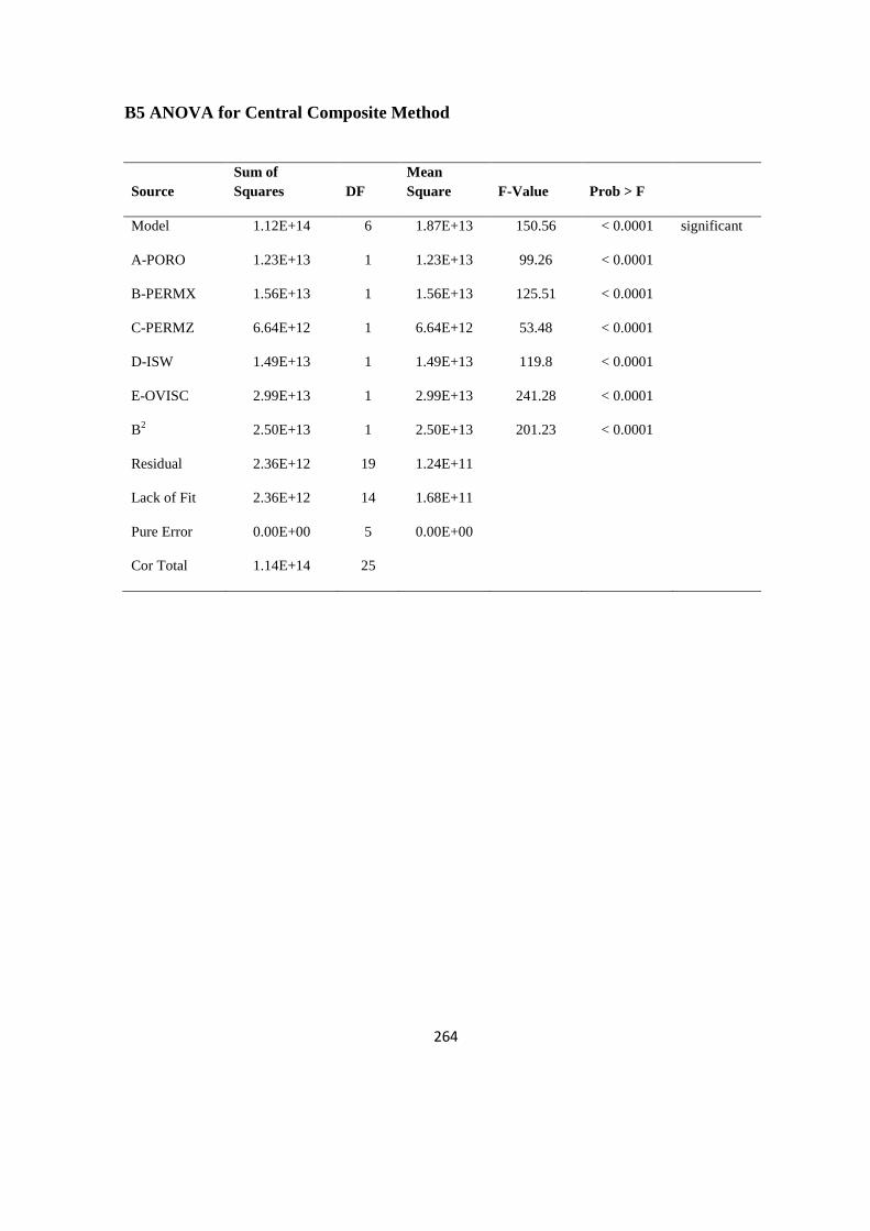
264
B5 ANOVA for Central Composite Method
Source
Sum of
Squares DF
Mean
Square F-Value Prob > F
Model 1.12E+14 6 1.87E+13 150.56 < 0.0001 significant
A-PORO 1.23E+13 1 1.23E+13 99.26 < 0.0001
B-PERMX 1.56E+13 1 1.56E+13 125.51 < 0.0001
C-PERMZ 6.64E+12 1 6.64E+12 53.48 < 0.0001
D-ISW 1.49E+13 1 1.49E+13 119.8 < 0.0001
E-OVISC 2.99E+13 1 2.99E+13 241.28 < 0.0001
B2 2.50E+13 1 2.50E+13 201.23 < 0.0001
Residual 2.36E+12 19 1.24E+11
Lack of Fit 2.36E+12 14 1.68E+11
Pure Error 0.00E+00 5 0.00E+00
Cor Total 1.14E+14 25
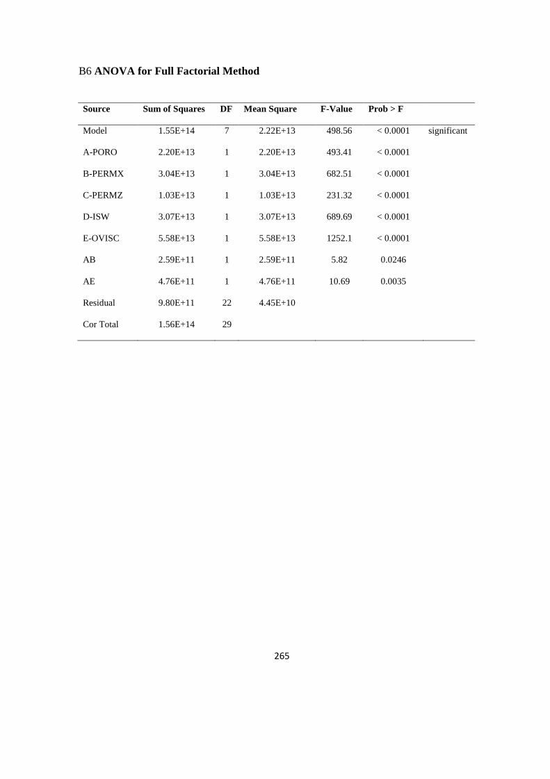
265
B6 ANOVA for Full Factorial Method
Source Sum of Squares DF Mean Square F-Value Prob > F
Model 1.55E+14 7 2.22E+13 498.56 < 0.0001 significant
A-PORO 2.20E+13 1 2.20E+13 493.41 < 0.0001
B-PERMX 3.04E+13 1 3.04E+13 682.51 < 0.0001
C-PERMZ 1.03E+13 1 1.03E+13 231.32 < 0.0001
D-ISW 3.07E+13 1 3.07E+13 689.69 < 0.0001
E-OVISC 5.58E+13 1 5.58E+13 1252.1 < 0.0001
AB 2.59E+11 1 2.59E+11 5.82 0.0246
AE 4.76E+11 1 4.76E+11 10.69 0.0035
Residual 9.80E+11 22 4.45E+10
Cor Total 1.56E+14 29
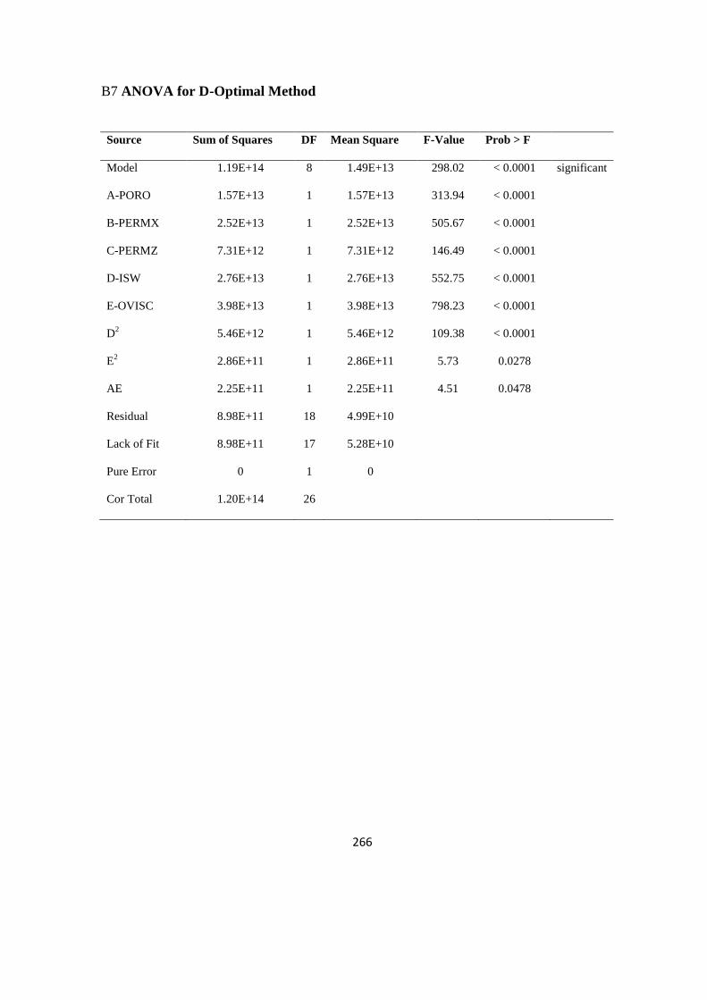
266
B7 ANOVA for D-Optimal Method
Source Sum of Squares DF Mean Square F-Value Prob > F
Model 1.19E+14 8 1.49E+13 298.02 < 0.0001 significant
A-PORO 1.57E+13 1 1.57E+13 313.94 < 0.0001
B-PERMX 2.52E+13 1 2.52E+13 505.67 < 0.0001
C-PERMZ 7.31E+12 1 7.31E+12 146.49 < 0.0001
D-ISW 2.76E+13 1 2.76E+13 552.75 < 0.0001
E-OVISC 3.98E+13 1 3.98E+13 798.23 < 0.0001
D2 5.46E+12 1 5.46E+12 109.38 < 0.0001
E2 2.86E+11 1 2.86E+11 5.73 0.0278
AE 2.25E+11 1 2.25E+11 4.51 0.0478
Residual 8.98E+11 18 4.99E+10
Lack of Fit 8.98E+11 17 5.28E+10
Pure Error 0 1 0
Cor Total 1.20E+14 26
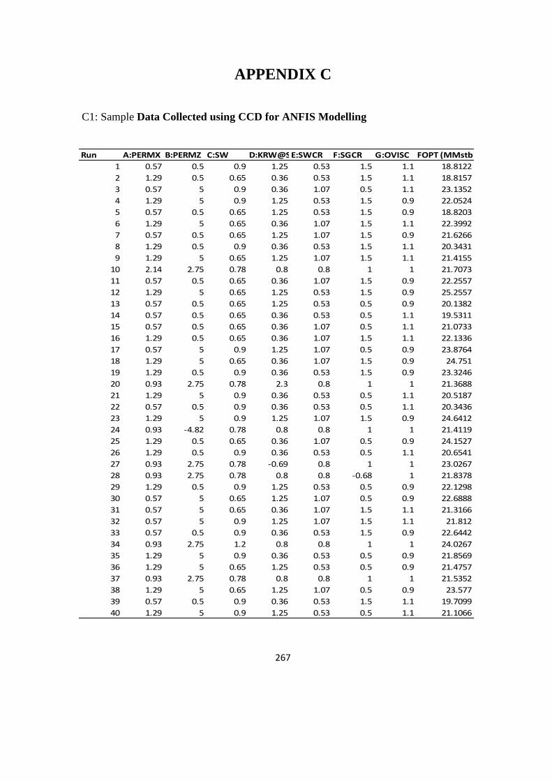
267
APPENDIX C
C1: Sample Data Collected using CCD for ANFIS Modelling
Run A:PERMX B:PERMZ C:SW D:KRW@SORWE:SWCR F:SGCR G:OVISC FOPT (MMstb)
1 0.57 0.5 0.9 1.25 0.53 1.5 1.1 18.8122
2 1.29 0.5 0.65 0.36 0.53 1.5 1.1 18.8157
3 0.57 5 0.9 0.36 1.07 0.5 1.1 23.1352
4 1.29 5 0.9 1.25 0.53 1.5 0.9 22.0524
5 0.57 0.5 0.65 1.25 0.53 1.5 0.9 18.8203
6 1.29 5 0.65 0.36 1.07 1.5 1.1 22.3992
7 0.57 0.5 0.65 1.25 1.07 1.5 0.9 21.6266
8 1.29 0.5 0.9 0.36 0.53 1.5 1.1 20.3431
9 1.29 5 0.65 1.25 1.07 1.5 1.1 21.4155
10 2.14 2.75 0.78 0.8 0.8 1 1 21.7073
11 0.57 0.5 0.65 0.36 1.07 1.5 0.9 22.2557
12 1.29 5 0.65 1.25 0.53 1.5 0.9 25.2557
13 0.57 0.5 0.65 1.25 0.53 0.5 0.9 20.1382
14 0.57 0.5 0.65 0.36 0.53 0.5 1.1 19.5311
15 0.57 0.5 0.65 0.36 1.07 0.5 1.1 21.0733
16 1.29 0.5 0.65 0.36 1.07 1.5 1.1 22.1336
17 0.57 5 0.9 1.25 1.07 0.5 0.9 23.8764
18 1.29 5 0.65 0.36 1.07 1.5 0.9 24.751
19 1.29 0.5 0.9 0.36 0.53 1.5 0.9 23.3246
20 0.93 2.75 0.78 2.3 0.8 1 1 21.3688
21 1.29 5 0.9 0.36 0.53 0.5 1.1 20.5187
22 0.57 0.5 0.9 0.36 0.53 0.5 1.1 20.3436
23 1.29 5 0.9 1.25 1.07 1.5 0.9 24.6412
24 0.93 -4.82 0.78 0.8 0.8 1 1 21.4119
25 1.29 0.5 0.65 0.36 1.07 0.5 0.9 24.1527
26 1.29 0.5 0.9 0.36 0.53 0.5 1.1 20.6541
27 0.93 2.75 0.78 -0.69 0.8 1 1 23.0267
28 0.93 2.75 0.78 0.8 0.8 -0.68 1 21.8378
29 1.29 0.5 0.9 1.25 0.53 0.5 0.9 22.1298
30 0.57 5 0.65 1.25 1.07 0.5 0.9 22.6888
31 0.57 5 0.65 0.36 1.07 1.5 1.1 21.3166
32 0.57 5 0.9 1.25 1.07 1.5 1.1 21.812
33 0.57 0.5 0.9 0.36 0.53 1.5 0.9 22.6442
34 0.93 2.75 1.2 0.8 0.8 1 1 24.0267
35 1.29 5 0.9 0.36 0.53 0.5 0.9 21.8569
36 1.29 5 0.65 1.25 0.53 0.5 0.9 21.4757
37 0.93 2.75 0.78 0.8 0.8 1 1 21.5352
38 1.29 5 0.65 1.25 1.07 0.5 0.9 23.577
39 0.57 0.5 0.9 0.36 0.53 1.5 1.1 19.7099
40 1.29 5 0.9 1.25 0.53 0.5 1.1 21.1066

268
C1 Continued
Run A:PERMX B:PERMZ C:SW D:KRW@SORWE:SWCR F:SGCR G:OVISC FOPT (MMstb)
41 1.29 0.5 0.9 1.25 1.07 1.5 1.1 21.907
42 1.29 5 0.65 0.36 0.53 1.5 0.9 20.7368
43 0.93 2.75 0.78 0.8 -0.11 1 1 19.0473
44 0.57 0.5 0.9 1.25 1.07 0.5 1.1 21.4696
45 0.57 0.5 0.65 1.25 1.07 0.5 1.1 20.7338
46 1.29 0.5 0.65 0.36 0.53 1.5 0.9 20.6415
47 1.29 0.5 0.65 0.36 0.53 0.5 1.1 19.8321
48 0.57 0.5 0.65 1.25 1.07 0.5 0.9 21.9283
49 0.57 5 0.9 0.36 0.53 1.5 1.1 19.8473
50 -0.28 2.75 0.78 0.8 0.8 1 1 20.667
51 0.57 5 0.65 1.25 1.07 1.5 0.9 22.6415
52 1.29 0.5 0.65 1.25 0.53 0.5 0.9 20.9744
53 1.29 5 0.65 1.25 0.53 0.5 1.1 20.3529
54 0.57 0.5 0.9 0.36 0.53 0.5 0.9 21.319
55 1.29 0.5 0.9 1.25 0.53 0.5 1.1 20.7658
56 1.29 5 0.65 0.36 0.53 0.5 1.1 20.3391
57 1.29 0.5 0.65 1.25 1.07 1.5 0.9 22.335
58 1.29 5 0.9 0.36 1.07 1.5 0.9 26.0848
59 1.29 5 0.9 1.25 1.07 0.5 1.1 22.5086
60 0.93 2.75 0.78 0.8 0.8 1 0.66 23.3181
61 0.57 5 0.65 0.36 0.53 0.5 0.9 20.7989
62 0.57 0.5 0.9 0.36 1.07 0.5 0.9 24.4832
63 0.57 5 0.9 0.36 0.53 1.5 0.9 20.9042
64 0.57 0.5 0.9 1.25 0.53 1.5 0.9 20.5857
65 1.29 5 0.65 0.36 0.53 1.5 1.1 19.4279
66 0.57 5 0.65 1.25 0.53 1.5 1.1 18.804
67 0.57 5 0.9 1.25 0.53 0.5 0.9 22.49
68 0.57 5 0.9 0.36 0.53 0.5 1.1 20.6541
69 0.57 5 0.9 0.36 1.07 1.5 1.1 22.6961
70 0.57 5 0.9 1.25 0.53 0.5 1.1 20.6307
71 0.57 5 0.65 1.25 0.53 0.5 0.9 20.1382
72 0.57 5 0.65 1.25 0.53 1.5 0.9 18.8273
73 1.29 0.5 0.9 1.25 0.53 1.5 1.1 20.4642
74 0.57 5 0.65 1.25 1.07 1.5 1.1 20.4327
75 0.57 0.5 0.9 0.36 1.07 0.5 1.1 22.501
76 1.29 5 0.9 0.36 1.07 0.5 0.9 26.5719
77 1.29 0.5 0.9 0.36 1.07 1.5 1.1 23.0481
78 1.29 5 0.9 0.36 1.07 0.5 1.1 23.7883
79 0.57 0.5 0.65 1.25 0.53 0.5 1.1 25.5719
80 0.57 5 0.9 1.25 1.07 0.5 1.1 22.0995
81 0.57 0.5 0.9 1.25 1.07 1.5 1.1 20.9552
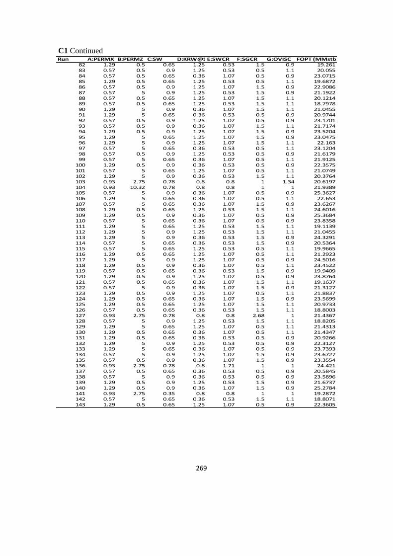
269
C1 Continued
Run A:PERMX B:PERMZ C:SW D:KRW@SORWE:SWCR F:SGCR G:OVISC FOPT (MMstb)82 1.29 0.5 0.65 1.25 0.53 1.5 0.9 19.26183 0.57 0.5 0.9 1.25 0.53 0.5 1.1 20.05584 0.57 0.5 0.65 0.36 1.07 0.5 0.9 23.071585 1.29 0.5 0.65 1.25 0.53 0.5 1.1 19.687286 0.57 0.5 0.9 1.25 1.07 1.5 0.9 22.908687 0.57 5 0.9 1.25 0.53 1.5 0.9 21.192288 0.57 0.5 0.65 1.25 1.07 1.5 1.1 20.121489 0.57 0.5 0.65 1.25 0.53 1.5 1.1 18.797890 1.29 5 0.9 0.36 1.07 1.5 1.1 21.045591 1.29 5 0.65 0.36 0.53 0.5 0.9 20.974492 0.57 0.5 0.9 1.25 1.07 0.5 0.9 23.170193 0.57 0.5 0.9 0.36 1.07 1.5 1.1 21.717494 1.29 0.5 0.9 1.25 1.07 1.5 0.9 23.520495 1.29 5 0.65 1.25 1.07 1.5 0.9 23.047596 1.29 5 0.9 1.25 1.07 1.5 1.1 22.16397 0.57 5 0.65 0.36 0.53 0.5 1.1 23.120498 0.57 0.5 0.9 1.25 0.53 0.5 0.9 21.617999 0.57 5 0.65 0.36 1.07 0.5 1.1 21.9125
100 1.29 0.5 0.9 0.36 0.53 0.5 0.9 22.3575101 0.57 5 0.65 1.25 1.07 0.5 1.1 21.0749102 1.29 5 0.9 0.36 0.53 1.5 1.1 20.3764103 0.93 2.75 0.78 0.8 0.8 1 1.34 20.6197104 0.93 10.32 0.78 0.8 0.8 1 1 21.9389105 0.57 5 0.9 0.36 1.07 0.5 0.9 25.3627106 1.29 5 0.65 0.36 1.07 0.5 1.1 22.653107 0.57 5 0.65 0.36 1.07 1.5 0.9 23.6267108 1.29 0.5 0.65 1.25 0.53 1.5 1.1 24.6016109 1.29 0.5 0.9 0.36 1.07 0.5 0.9 25.3684110 0.57 5 0.65 0.36 1.07 0.5 0.9 23.8358111 1.29 5 0.65 1.25 0.53 1.5 1.1 19.1139112 1.29 5 0.9 1.25 0.53 1.5 1.1 21.0455113 1.29 5 0.9 0.36 0.53 1.5 0.9 24.3291114 0.57 5 0.65 0.36 0.53 1.5 0.9 20.5364115 0.57 5 0.65 1.25 0.53 0.5 1.1 19.9665116 1.29 0.5 0.65 1.25 1.07 0.5 1.1 21.2923117 1.29 5 0.9 1.25 1.07 0.5 0.9 24.5016118 1.29 0.5 0.9 0.36 1.07 0.5 1.1 23.4522119 0.57 0.5 0.65 0.36 0.53 1.5 0.9 19.9409120 1.29 0.5 0.9 1.25 1.07 0.5 0.9 23.8764121 0.57 0.5 0.65 0.36 1.07 1.5 1.1 19.1637122 0.57 5 0.9 0.36 1.07 1.5 0.9 21.3127123 1.29 0.5 0.9 1.25 1.07 0.5 1.1 21.8837124 1.29 0.5 0.65 0.36 1.07 1.5 0.9 23.5699125 1.29 0.5 0.65 1.25 1.07 1.5 1.1 20.9733126 0.57 0.5 0.65 0.36 0.53 1.5 1.1 18.8003127 0.93 2.75 0.78 0.8 0.8 2.68 1 21.4367128 0.57 5 0.9 1.25 0.53 1.5 1.1 18.8205129 1.29 5 0.65 1.25 1.07 0.5 1.1 21.4313130 1.29 0.5 0.65 0.36 1.07 0.5 1.1 21.4347131 1.29 0.5 0.65 0.36 0.53 0.5 0.9 20.9266132 1.29 5 0.9 1.25 0.53 0.5 0.9 22.3127133 1.29 5 0.65 0.36 1.07 0.5 0.9 23.7393134 0.57 5 0.9 1.25 1.07 1.5 0.9 23.6727135 0.57 0.5 0.9 0.36 1.07 1.5 0.9 23.3554136 0.93 2.75 0.78 0.8 1.71 1 1 24.421137 0.57 0.5 0.65 0.36 0.53 0.5 0.9 20.5845138 0.57 5 0.9 0.36 0.53 0.5 0.9 23.5896139 1.29 0.5 0.9 1.25 0.53 1.5 0.9 21.6737140 1.29 0.5 0.9 0.36 1.07 1.5 0.9 25.2784141 0.93 2.75 0.35 0.8 0.8 1 1 19.2872142 0.57 5 0.65 0.36 0.53 1.5 1.1 18.8071143 1.29 0.5 0.65 1.25 1.07 0.5 0.9 22.3605

270
C2: CCD Matrix for development of EQ. 3.1
Run PHIE SW NTG OWC Thickness STOIIP (MMSTB)Run PHIE SW NTG OWC Thickness STOIIP (MMSTB)
1 1 -1 1 1 -1 54 26 1 1 -1 1 -1 61
2 -1 -1 1 -1 1 41 27 1 -1 1 -1 1 46
3 0 0 0 0 0 48 28 -1 1 -1 -1 1 50
4 0 0 0 0 0 47 29 0 0 2 0 0 54
5 2 0 0 0 0 54 30 0 0 0 0 0 65
6 1 1 -1 -1 -1 54 31 1 1 1 1 -1 41
7 -1 1 1 1 1 48 32 1 1 1 1 1 56
8 -2 0 0 0 0 59 33 -1 -1 -1 -1 -1 68
9 0 0 0 0 2 50 34 0 0 0 0 0 54
10 1 -1 -1 -1 -1 59 35 1 1 -1 -1 1 40
11 1 -1 1 1 1 44 36 1 1 -1 1 1 54
12 -1 -1 1 1 1 44 37 -1 1 -1 -1 -1 56
13 -1 1 -1 1 1 54 38 0 2 0 0 0 59
14 0 -2 0 0 0 45 39 0 0 0 0 -2 48
15 0 0 0 0 0 53 40 -1 1 -1 1 -1 54
16 0 0 0 0 0 54 41 -1 -1 -1 -1 1 54
17 -1 -1 -1 1 -1 54 42 1 -1 -1 1 -1 54
18 0 0 0 0 0 65 43 -1 -1 -1 1 1 48
19 -1 1 1 -1 -1 49 44 1 -1 -1 1 1 53
20 -1 -1 1 1 -1 54 45 1 1 1 -1 1 66
21 1 -1 1 -1 -1 54 46 1 -1 -1 -1 1 54
22 0 0 0 -2 0 62 47 0 0 0 2 0 48
23 1 1 1 -1 -1 53 48 -1 1 1 1 -1 56
24 0 0 0 0 0 55 49 -1 1 1 -1 1 54
25 -1 -1 1 -1 -1 40 50 0 0 -2 0 0 40
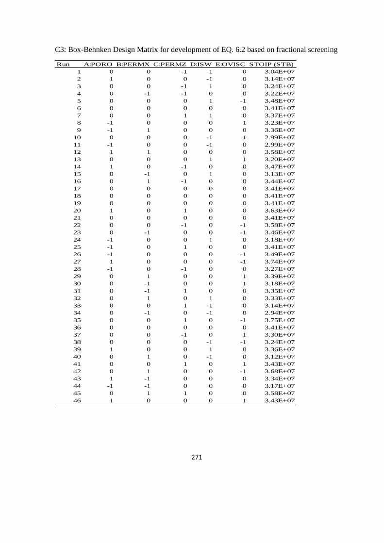
271
C3: Box-Behnken Design Matrix for development of EQ. 6.2 based on fractional screening
Run A:PORO B:PERMX C:PERMZ D:ISW E:OVISC STOIP (STB)
1 0 0 -1 -1 0 3.04E+07
2 1 0 0 -1 0 3.14E+07
3 0 0 -1 1 0 3.24E+07
4 0 -1 -1 0 0 3.22E+07
5 0 0 0 1 -1 3.48E+07
6 0 0 0 0 0 3.41E+07
7 0 0 1 1 0 3.37E+07
8 -1 0 0 0 1 3.23E+07
9 -1 1 0 0 0 3.36E+07
10 0 0 0 -1 1 2.99E+07
11 -1 0 0 -1 0 2.99E+07
12 1 1 0 0 0 3.58E+07
13 0 0 0 1 1 3.20E+07
14 1 0 -1 0 0 3.47E+07
15 0 -1 0 1 0 3.13E+07
16 0 1 -1 0 0 3.44E+07
17 0 0 0 0 0 3.41E+07
18 0 0 0 0 0 3.41E+07
19 0 0 0 0 0 3.41E+07
20 1 0 1 0 0 3.63E+07
21 0 0 0 0 0 3.41E+07
22 0 0 -1 0 -1 3.58E+07
23 0 -1 0 0 -1 3.46E+07
24 -1 0 0 1 0 3.18E+07
25 -1 0 1 0 0 3.41E+07
26 -1 0 0 0 -1 3.49E+07
27 1 0 0 0 -1 3.74E+07
28 -1 0 -1 0 0 3.27E+07
29 0 1 0 0 1 3.39E+07
30 0 -1 0 0 1 3.18E+07
31 0 -1 1 0 0 3.35E+07
32 0 1 0 1 0 3.33E+07
33 0 0 1 -1 0 3.14E+07
34 0 -1 0 -1 0 2.94E+07
35 0 0 1 0 -1 3.75E+07
36 0 0 0 0 0 3.41E+07
37 0 0 -1 0 1 3.30E+07
38 0 0 0 -1 -1 3.24E+07
39 1 0 0 1 0 3.36E+07
40 0 1 0 -1 0 3.12E+07
41 0 0 1 0 1 3.43E+07
42 0 1 0 0 -1 3.68E+07
43 1 -1 0 0 0 3.34E+07
44 -1 -1 0 0 0 3.17E+07
45 0 1 1 0 0 3.58E+07
46 1 0 0 0 1 3.43E+07

272
C4: CCD Matrix for development of EQ. 6.3 based on fractional factorial screening
Run A:PORO B:PERMXC:PERMZ D:ISW E:OVISC STOIIP(STB)
1 0 0 0 0 0 3.41E+07
2 0 0 0 0 2 3.33E+07
3 -1 1 -1 -1 -1 3.19E+07
4 -2 0 0 0 0 3.31E+07
5 0 0 2 0 0 3.52E+07
6 1 1 1 -1 -1 3.52E+07
7 -1 -1 -1 1 -1 3.19E+07
8 0 0 0 0 0 3.41E+07
9 1 1 -1 -1 1 3.09E+07
10 0 0 -2 0 0 3.38E+07
11 1 1 1 1 1 3.43E+07
12 0 -2 0 0 0 3.26E+07
13 0 0 0 2 0 3.27E+07
14 0 2 0 0 0 3.47E+07
15 -1 1 1 1 -1 3.52E+07
16 0 0 0 0 0 3.41E+07
17 0 0 0 -2 0 3.06E+07
18 1 1 -1 1 -1 3.61E+07
19 -1 1 1 -1 1 3.30E+07
20 0 0 0 0 0 3.41E+07
21 1 -1 1 -1 1 3.01E+07
22 -1 -1 1 -1 -1 3.11E+07
23 0 0 0 0 0 3.41E+07
24 -1 -1 1 1 1 3.05E+07
25 0 0 0 0 0 3.41E+07
26 1 -1 -1 -1 -1 3.15E+07
27 1 -1 -1 1 1 3.08E+07
28 2 0 0 0 0 3.51E+07
29 0 0 0 0 -2 3.62E+07
30 1 -1 1 1 -1 3.52E+07
31 -1 1 -1 1 1 3.13E+07
32 -1 -1 -1 -1 1 2.79E+07
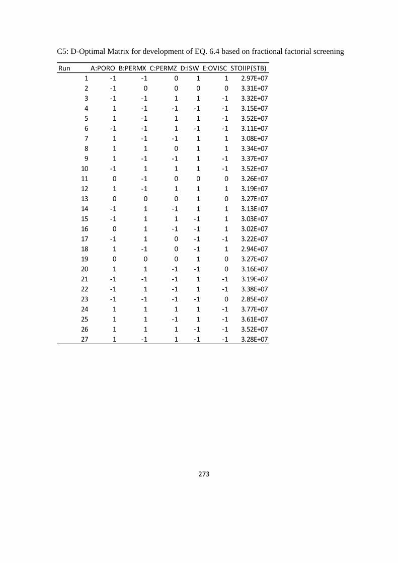
273
C5: D-Optimal Matrix for development of EQ. 6.4 based on fractional factorial screening
Run A:PORO B:PERMX C:PERMZ D:ISW E:OVISC STOIIP(STB)
1 -1 -1 0 1 1 2.97E+07
2 -1 0 0 0 0 3.31E+07
3 -1 -1 1 1 -1 3.32E+07
4 1 -1 -1 -1 -1 3.15E+07
5 1 -1 1 1 -1 3.52E+07
6 -1 -1 1 -1 -1 3.11E+07
7 1 -1 -1 1 1 3.08E+07
8 1 1 0 1 1 3.34E+07
9 1 -1 -1 1 -1 3.37E+07
10 -1 1 1 1 -1 3.52E+07
11 0 -1 0 0 0 3.26E+07
12 1 -1 1 1 1 3.19E+07
13 0 0 0 1 0 3.27E+07
14 -1 1 -1 1 1 3.13E+07
15 -1 1 1 -1 1 3.03E+07
16 0 1 -1 -1 1 3.02E+07
17 -1 1 0 -1 -1 3.22E+07
18 1 -1 0 -1 1 2.94E+07
19 0 0 0 1 0 3.27E+07
20 1 1 -1 -1 0 3.16E+07
21 -1 -1 -1 1 -1 3.19E+07
22 -1 1 -1 1 -1 3.38E+07
23 -1 -1 -1 -1 0 2.85E+07
24 1 1 1 1 -1 3.77E+07
25 1 1 -1 1 -1 3.61E+07
26 1 1 1 -1 -1 3.52E+07
27 1 -1 1 -1 -1 3.28E+07

274
C6: Factorial Design Matrix for development of EQ. 6.5 based on fractional factorial
screening
Run A:PORO B:PERMX C:PERMZ D:ISW E:OVISC STOIIP(STB)
1 -1 -1 -1 1 1 3.00E+07
2 -1 1 -1 1 1 3.15E+07
3 -1 1 1 -1 -1 3.19E+07
4 -1 -1 1 -1 1 3.38E+07
5 -1 1 -1 -1 -1 3.11E+07
6 -1 -1 1 1 -1 3.28E+07
7 1 -1 -1 1 -1 3.30E+07
8 1 -1 -1 1 1 3.52E+07
9 1 -1 1 -1 -1 3.19E+07
10 1 -1 -1 -1 -1 3.37E+07
11 -1 1 -1 1 -1 3.38E+07
12 -1 -1 -1 1 -1 3.61E+07
13 -1 -1 1 -1 -1 3.32E+07
14 1 1 1 -1 1 3.52E+07
15 1 -1 1 -1 1 3.52E+07
16 1 1 1 -1 -1 3.77E+07
17 -1 1 -1 -1 1 2.79E+07
18 1 1 -1 -1 -1 2.91E+07
19 1 1 -1 1 1 2.94E+07
20 -1 1 1 1 1 3.09E+07
21 1 1 1 1 -1 2.88E+07
22 1 1 -1 -1 1 3.01E+07
23 1 -1 1 1 1 3.19E+07
24 -1 -1 1 1 1 2.94E+07
25 1 1 1 1 1 3.09E+07
26 -1 1 1 -1 1 3.13E+07
27 1 -1 1 1 -1 3.31E+07
28 1 -1 -1 -1 1 3.05E+07
29 -1 -1 -1 -1 1 3.19E+07
30 1 1 -1 1 -1 3.24E+07
31 -1 -1 -1 -1 -1 2.84E+07
32 -1 1 1 1 -1 3.14E+07

275
C7: Box-Behnken Design Matrix for development of EQ. 6.6 based on PB screening
Run A:PORO B:PERMX C:ISW D:OVISC STOIIP (STB)
1 0 0 0 0 3.17E+07
2 1 0 1 0 3.34E+07
3 0 0 1 1 3.36E+07
4 -1 0 -1 0 3.58E+07
5 1 0 -1 0 3.24E+07
6 0 0 0 0 3.48E+07
7 0 -1 0 1 2.99E+07
8 0 0 0 0 3.20E+07
9 -1 -1 0 0 3.49E+07
10 0 -1 0 -1 3.74E+07
11 1 1 0 0 3.23E+07
12 0 1 0 -1 3.43E+07
13 0 1 0 1 2.94E+07
14 1 -1 0 0 3.12E+07
15 -1 1 0 0 3.13E+07
16 0 -1 -1 0 3.33E+07
17 0 0 0 0 2.99E+07
18 0 1 -1 0 3.14E+07
19 0 -1 1 0 3.18E+07
20 0 0 -1 -1 3.36E+07
21 0 0 0 0 3.46E+07
22 0 0 -1 1 3.68E+07
23 0 1 1 0 3.18E+07
24 -1 0 0 1 3.39E+07
25 1 0 0 1 3.41E+07
26 -1 0 0 -1 3.41E+07
27 1 0 0 -1 3.41E+07
28 -1 0 1 0 3.41E+07

276
C8: Full Factorial Design Matrix for development of EQ. 6.7 based on PB screening
Run A:PORO B:PERMX C:ISW D:OVISC STOIIP (STB)
1 0 1 -1 1 3.03E+07
2 0 -1 -1 0 3.11E+07
3 0 1 -1 -1 3.18E+07
4 1 -1 1 1 3.15E+07
5 0 1 1 1 3.24E+07
6 1 1 -1 -1 3.33E+07
7 1 -1 1 -1 3.22E+07
8 -1 1 0 1 3.32E+07
9 -1 -1 -1 1 3.42E+07
10 1 0 0 1 3.35E+07
11 0 0 0 0 3.46E+07
12 -1 1 -1 1 3.56E+07
13 -1 0 0 0 3.49E+07
14 0 -1 0 0 3.62E+07
15 -1 0 1 1 3.74E+07
16 0 0 1 0 3.55E+07
17 1 1 0 0 3.68E+07
18 0 1 -1 0 3.81E+07
19 1 0 1 1 3.22E+07
20 1 0 0 -1 3.32E+07
21 0 1 0 1 3.41E+07
22 1 -1 -1 1 3.36E+07
23 -1 0 0 -1 3.48E+07
24 1 -1 0 1 3.58E+07
25 1 1 0 1 3.41E+07
26 1 0 1 -1 3.54E+07
27 -1 0 -1 1 3.65E+07
28 0 0 0 0 2.87E+07
29 0 0 -1 0 2.94E+07
30 1 1 1 0 3.00E+07
31 0 1 1 -1 2.99E+07
32 -1 1 1 1 3.06E+07
33 0 1 0 -1 3.14E+07
34 1 0 0 0 3.04E+07
35 1 1 1 1 3.12E+07
36 -1 0 1 -1 3.20E+07
37 -1 -1 1 0 3.17E+07
38 -1 0 -1 -1 3.26E+07
39 0 0 1 -1 3.34E+07
40 0 -1 0 -1 3.31E+07
41 0 -1 1 1 3.41E+07
42 0 0 0 -1 3.51E+07
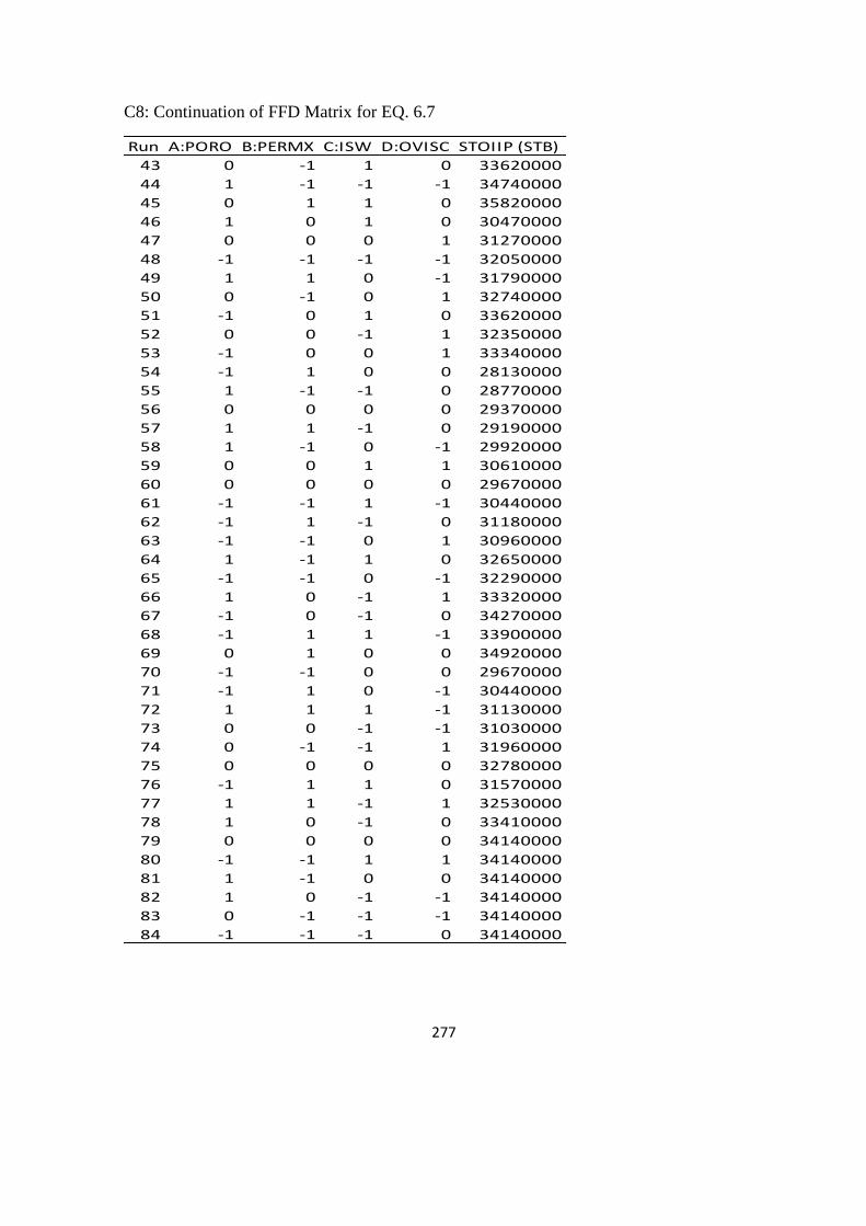
277
C8: Continuation of FFD Matrix for EQ. 6.7
Run A:PORO B:PERMX C:ISW D:OVISC STOIIP (STB)
43 0 -1 1 0 33620000
44 1 -1 -1 -1 34740000
45 0 1 1 0 35820000
46 1 0 1 0 30470000
47 0 0 0 1 31270000
48 -1 -1 -1 -1 32050000
49 1 1 0 -1 31790000
50 0 -1 0 1 32740000
51 -1 0 1 0 33620000
52 0 0 -1 1 32350000
53 -1 0 0 1 33340000
54 -1 1 0 0 28130000
55 1 -1 -1 0 28770000
56 0 0 0 0 29370000
57 1 1 -1 0 29190000
58 1 -1 0 -1 29920000
59 0 0 1 1 30610000
60 0 0 0 0 29670000
61 -1 -1 1 -1 30440000
62 -1 1 -1 0 31180000
63 -1 -1 0 1 30960000
64 1 -1 1 0 32650000
65 -1 -1 0 -1 32290000
66 1 0 -1 1 33320000
67 -1 0 -1 0 34270000
68 -1 1 1 -1 33900000
69 0 1 0 0 34920000
70 -1 -1 0 0 29670000
71 -1 1 0 -1 30440000
72 1 1 1 -1 31130000
73 0 0 -1 -1 31030000
74 0 -1 -1 1 31960000
75 0 0 0 0 32780000
76 -1 1 1 0 31570000
77 1 1 -1 1 32530000
78 1 0 -1 0 33410000
79 0 0 0 0 34140000
80 -1 -1 1 1 34140000
81 1 -1 0 0 34140000
82 1 0 -1 -1 34140000
83 0 -1 -1 -1 34140000
84 -1 -1 -1 0 34140000
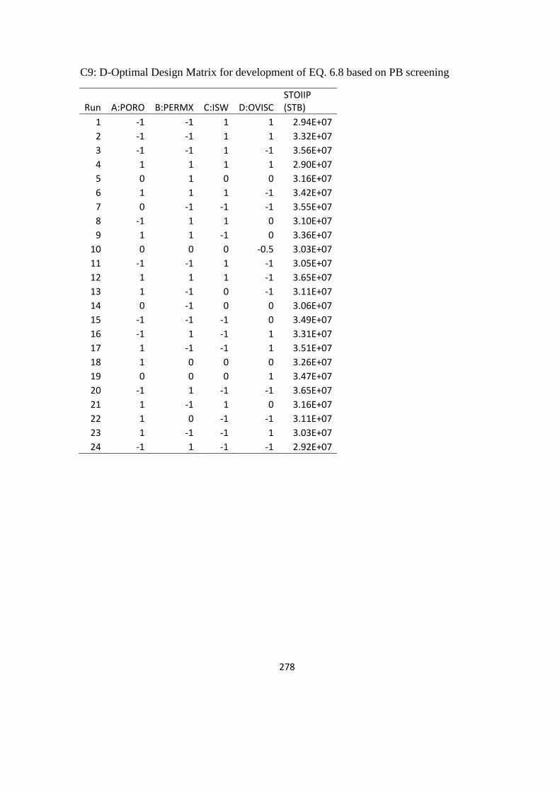
278
C9: D-Optimal Design Matrix for development of EQ. 6.8 based on PB screening
Run A:PORO B:PERMX C:ISW D:OVISC STOIIP (STB)
1 -1 -1 1 1 2.94E+07
2 -1 -1 1 1 3.32E+07
3 -1 -1 1 -1 3.56E+07
4 1 1 1 1 2.90E+07
5 0 1 0 0 3.16E+07
6 1 1 1 -1 3.42E+07
7 0 -1 -1 -1 3.55E+07
8 -1 1 1 0 3.10E+07
9 1 1 -1 0 3.36E+07
10 0 0 0 -0.5 3.03E+07
11 -1 -1 1 -1 3.05E+07
12 1 1 1 -1 3.65E+07
13 1 -1 0 -1 3.11E+07
14 0 -1 0 0 3.06E+07
15 -1 -1 -1 0 3.49E+07
16 -1 1 -1 1 3.31E+07
17 1 -1 -1 1 3.51E+07
18 1 0 0 0 3.26E+07
19 0 0 0 1 3.47E+07
20 -1 1 -1 -1 3.65E+07
21 1 -1 1 0 3.16E+07
22 1 0 -1 -1 3.11E+07
23 1 -1 -1 1 3.03E+07
24 -1 1 -1 -1 2.92E+07
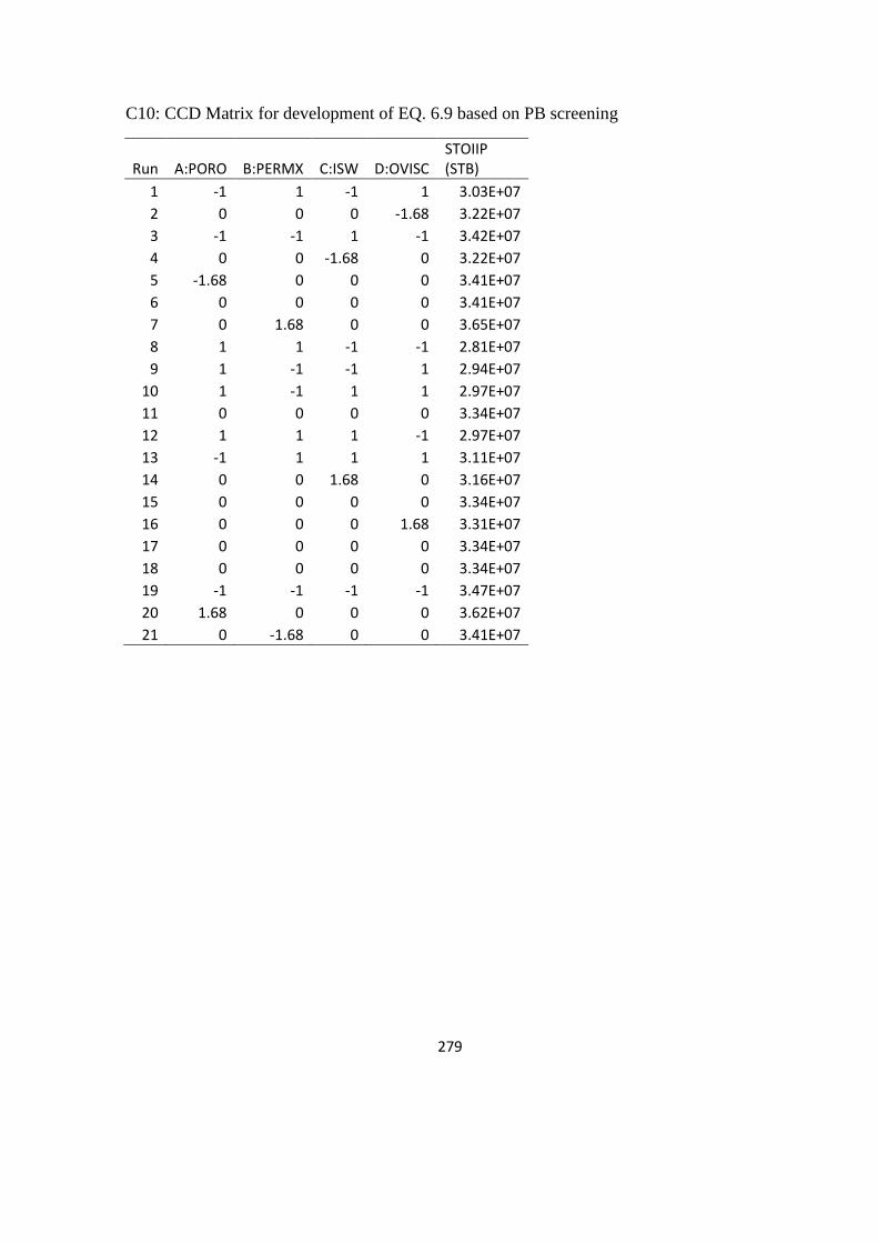
279
C10: CCD Matrix for development of EQ. 6.9 based on PB screening
Run A:PORO B:PERMX C:ISW D:OVISC STOIIP (STB)
1 -1 1 -1 1 3.03E+07
2 0 0 0 -1.68 3.22E+07
3 -1 -1 1 -1 3.42E+07
4 0 0 -1.68 0 3.22E+07
5 -1.68 0 0 0 3.41E+07
6 0 0 0 0 3.41E+07
7 0 1.68 0 0 3.65E+07
8 1 1 -1 -1 2.81E+07
9 1 -1 -1 1 2.94E+07
10 1 -1 1 1 2.97E+07
11 0 0 0 0 3.34E+07
12 1 1 1 -1 2.97E+07
13 -1 1 1 1 3.11E+07
14 0 0 1.68 0 3.16E+07
15 0 0 0 0 3.34E+07
16 0 0 0 1.68 3.31E+07
17 0 0 0 0 3.34E+07
18 0 0 0 0 3.34E+07
19 -1 -1 -1 -1 3.47E+07
20 1.68 0 0 0 3.62E+07
21 0 -1.68 0 0 3.41E+07
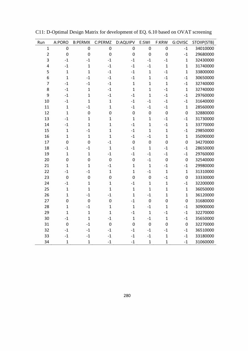
280
C11: D-Optimal Design Matrix for development of EQ. 6.10 based on OVAT screening
Run A:PORO B:PERMX C:PERMZ D:AQUIPV E:SWI F:KRW G:OVISC STOIIP(STB)
1 0 0 0 0 0 0 -1 34010000
2 0 0 0 0 0 0 -1 29680000
3 -1 -1 -1 -1 -1 -1 1 32430000
4 -1 1 -1 -1 -1 1 1 31740000
5 1 1 -1 -1 1 -1 1 33800000
6 1 -1 -1 -1 1 -1 -1 30650000
7 -1 -1 -1 1 1 1 -1 32740000
8 -1 1 -1 1 1 -1 1 32740000
9 -1 1 -1 -1 1 -1 -1 29760000
10 -1 1 1 -1 -1 -1 -1 31640000
11 1 -1 1 -1 -1 -1 1 28560000
12 1 0 0 0 0 0 0 32880000
13 -1 1 1 1 1 -1 -1 31730000
14 -1 1 1 -1 1 -1 1 33770000
15 1 -1 1 -1 1 1 -1 29850000
16 1 1 1 -1 -1 1 1 35090000
17 0 0 -1 0 0 0 0 34270000
18 -1 -1 1 -1 1 -1 -1 28650000
19 1 1 -1 -1 -1 -1 -1 29760000
20 0 0 0 0 -1 0 0 32540000
21 1 1 -1 1 1 -1 -1 29980000
22 -1 -1 1 1 -1 1 1 31310000
23 0 0 0 0 0 -1 0 33330000
24 -1 1 1 -1 1 1 -1 32200000
25 1 1 1 1 1 1 1 36050000
26 1 -1 -1 1 -1 1 1 36120000
27 0 0 0 -1 0 0 0 31680000
28 1 -1 1 1 -1 1 -1 30900000
29 1 1 1 -1 1 -1 -1 32270000
30 -1 1 -1 1 -1 1 -1 35650000
31 0 -1 0 0 0 0 0 32270000
32 -1 -1 -1 -1 -1 -1 -1 36510000
33 -1 -1 -1 -1 -1 1 -1 33180000
34 1 1 -1 -1 1 1 -1 31060000
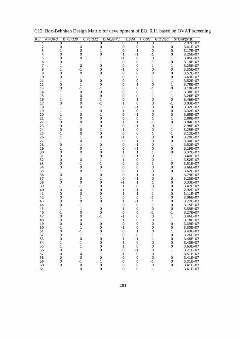
281
C12: Box-Behnken Design Matrix for development of EQ. 6.11 based on OVAT screening
Run A:PORO B:PERMX C:PERMZ D:AQUIPV E:SWI F:KRW G:OVISC STOIIP(STB)1 0 -1 0 0 1 0 -1 2.97E+072 0 0 0 0 0 0 0 3.41E+073 -1 0 1 0 1 0 0 3.17E+074 0 0 0 1 -1 -1 0 3.25E+075 0 0 1 -1 0 0 1 3.05E+076 0 1 -1 0 0 -1 0 3.14E+077 1 0 0 0 0 -1 1 3.25E+078 1 -1 0 -1 0 0 0 3.35E+079 0 0 0 0 0 0 0 3.57E+07
10 0 1 -1 0 0 1 0 3.69E+0711 -1 0 0 0 0 -1 1 3.52E+0712 0 1 0 0 1 0 1 3.78E+0713 0 -1 -1 0 0 -1 0 3.19E+0714 1 0 0 0 0 1 -1 3.38E+0715 1 0 0 0 0 1 1 3.26E+0716 1 0 -1 0 1 0 0 3.46E+0717 0 0 -1 1 0 0 -1 3.03E+0718 1 0 1 0 -1 0 0 3.32E+0719 -1 -1 0 -1 0 0 0 3.32E+0720 1 0 -1 0 -1 0 0 3.65E+0721 -1 0 0 0 0 1 1 2.88E+0722 0 0 0 1 1 -1 0 3.04E+0723 0 -1 0 0 -1 0 1 2.98E+0724 0 0 1 1 0 0 1 3.25E+0725 -1 0 0 0 0 1 -1 3.12E+0726 1 1 0 -1 0 0 0 3.20E+0727 -1 0 -1 0 1 0 0 3.30E+0728 0 -1 0 0 -1 0 -1 3.52E+0729 -1 0 1 0 -1 0 0 3.19E+0730 0 0 0 1 1 1 0 3.37E+0731 0 1 0 0 -1 0 -1 3.40E+0732 0 0 1 -1 0 0 -1 3.52E+0733 0 -1 -1 0 0 1 0 3.51E+0734 0 0 0 0 0 0 0 3.66E+0735 1 0 1 0 1 0 0 3.62E+0736 0 1 0 0 1 0 -1 3.79E+0737 -1 0 -1 0 -1 0 0 3.23E+0738 0 0 0 -1 1 1 0 3.33E+0739 -1 -1 0 1 0 0 0 3.47E+0740 0 0 0 -1 -1 -1 0 2.92E+0741 0 0 0 -1 1 -1 0 3.11E+0742 0 1 1 0 0 -1 0 3.06E+0743 0 0 0 1 -1 1 0 3.22E+0744 0 -1 1 0 0 1 0 3.15E+0745 -1 1 0 1 0 0 0 3.33E+0746 -1 0 0 0 0 -1 -1 3.27E+0747 0 0 -1 -1 0 0 1 3.46E+0748 0 0 1 1 0 0 -1 3.18E+0749 0 0 0 0 0 0 0 3.39E+0750 -1 1 0 -1 0 0 0 3.30E+0751 0 -1 0 0 1 0 1 3.43E+0752 0 1 1 0 0 1 0 3.26E+0753 0 0 0 -1 -1 1 0 3.48E+0754 1 -1 0 1 0 0 0 3.40E+0755 1 1 0 1 0 0 0 3.63E+0756 0 1 0 0 -1 0 1 3.21E+0757 0 0 -1 -1 0 0 -1 3.51E+0758 0 0 0 0 0 0 0 3.41E+0759 0 -1 1 0 0 -1 0 3.31E+0760 0 0 0 0 0 0 0 3.41E+0761 1 0 0 0 0 -1 -1 3.61E+07