uncertainty analysis for the integration of seismic and ...derived from integration of seismic and...
TRANSCRIPT

CWP-623
Uncertainty analysis for the integration of seismic and
CSEM data
Myoung Jae Kwon & Roel SniederCenter for Wave Phenomena, Colorado School of Mines
ABSTRACT
Geophysical inverse problems consist of three stages: the forward problem, opti-mization, and appraisal. We study the appraisal problem for the joint inversionof seismic and controlled source electro-magnetic (CSEM) data and utilize rock-physics models to integrate these two disparate data sets. The appraisal problemis solved by adopting a Bayesian model and we incorporate four representativesources of uncertainty. These are uncertainties in (1) seismic wave velocity, (2)electric conductivity, (3) seismic data, and (4) CSEM data. The uncertainties inporosity and water saturation are quantified by a posterior random sampling inthe model space of porosity and water saturation of a marine one-dimensionalstructure. We study the relative contributions from the four individual sourcesof uncertainty by performing several statistical experiments. The uncertaintiesin the seismic wave velocity and electric conductivity play a more significant roleon the variation of posterior uncertainty than do the seismic and CSEM datanoise. The numerical simulations also show that the assessment of porosity ismost affected by the uncertainty in seismic wave velocity and the assessment ofwater saturation is most influenced by the uncertainty in electric conductivity.The framework of the uncertainty analysis presented in this study can be uti-lized to effectively reduce the uncertainty of the porosity and water saturationderived from integration of seismic and CSEM data.
Key words: uncertainty analysis, Metropolis-Hastings algorithm, CSEM
1 INTRODUCTION
Currently, there is an increasing interest in the inte-gration of the seismic and controlled source electro-magnetic (CSEM) method in deep marine exploration(Harris & MacGregor, 2006). Although the CSEMmethod has less resolution than the seismic method, itprovides extra information about, for example, electricconductivity. This property is important for the eco-nomic evaluation of reservoirs. Therefore, the CSEMmethod is considered an effective complementary toolwhen combined with seismic exploration.
The seismic and CSEM methods are disparateexploration techniques that are sensitive to differentmedium properties: the seismic method is sensitiveto density and seismic wave velocity and the CSEMmethod to electric conductivity. There have been several
approaches for joint inversion that integrate disparatedata sets. Some of them assume a common structure(Musil et al., 2003) or similar structural variations ofdifferent medium properties (Gallardo & Meju, 2004).More recently, the application of rock-physics modelsfor joint inversion has been studied (Hoversten et al.,2006). Rock-physics models enable us to interrelate seis-mic wave velocity and electric conductivity with thereservoir parameters such as porosity, water saturation,or permeability. The main advantage of the approachis that the reservoir parameters have great economicimportance. The application of a rock-physics model islimited, however, by the fact that such a model is site-specific and there are not yet any universal solutions tothe inverse problem. Furthermore, even for any partic-ular area of interest, any rock-physics model is gener-ally described as a cloud of samples. These limitations

52 M.J. Kwon & R. Snieder
Figure 1. Division of an inverse problem into a forwardproblem, an optimization problem, and an appraisal prob-
lem.
imply that joint inversion via a rock-physics model in-trinsically necessitates a stochastic approach. Stochasticinversion has recently been studied for seismic inversion(Spikes et al., 2007) and joint inversion of seismic andCSEM data (Chen et al., 2007). However, the contribu-tions of rock-physics model uncertainties are not yet wellunderstood. In fact, the accuracy of our joint inversionis limited by the uncertainty of rock-physics model aswell as by the data noise. We therefore model both thedata noise and the uncertainty of rock-physics modelsin this research.
In many geophysical inverse problems, we have fi-nite data and retrieve a model that has infinitely manydegrees of freedom (Snieder, 1998). So far, most of thegeophysical inversion studies have concentrated on find-ing the model that best fits the data; this is an op-timization problem. In this research we quantify howmuch confidence we can place in the optimum solution;this is an appraisal problem. The appraisal problem hasparticular significance when the rock-physics model isused for the joint inversion of the seismic and CSEMdata. We investigate the relative contribution of differ-ent sources of overall uncertainty that arise when we userock-physics models for the joint inversion. These in-clude seismic data noise, CSEM data noise, and uncer-tainties of rock-physics models. We implement severalnumerical experiments that reflect scenarios we may en-counter in practice and compare the uncertainties in theinferred parameters. The comparison reveals the relativecontributions of different sources of uncertainty and wecan utilize the procedure to more effectively reduce theuncertainty, depending on whether our interests focuson porosity or water saturation.
2 METHODOLOGY
The goal of geophysical inversion is to make quantitativeinferences about the earth from noisy data. There are
mainly two different approaches for attaining this goal:in one the unknown models are assumed deterministicand one uses inversion methods such as Tikhonov regu-larization; in the other all the unknowns are random andone uses Bayesian methods. The object of this projectis to provide a framework for Bayesian joint inversionthat leads to model estimates and their uncertainties.
The connection between geophysical data d andmodel m is written as
d = L[m] + e (1)
where L denotes a linear or nonlinear operator thatmaps the model into the data and e represents datameasurement error. The details of the operator are pre-sented in the modeling procedure section. Bayes’ the-orem relates conditional and marginal probabilities ofa data d and a model m as follows (Scales & Snieder,1997; Sivia & Webster, 1998):
π(m|d) =π(m)f(d|m)
π(d)∝ π(m)f(d|m), (2)
where π(m) is a prior probability in the sense that itdoes not take into account any information about thedata d; f(d|m) is likelihood of the data d, given a modelm; and π(m|d) is a posterior probability density thatwe are inferring. The denominator of equation (2) is theprobability distribution of the data d. This quantity canbe written as π(d) =
R
π(m)f(d|m) dm. In practicalapplications, the denominator is not evaluated and therelative change of the posterior probability as a functionof the model parameter is investigated.
2.1 Hierarchical Bayesian model
The P -wave velocity and electric conductivity are de-rived from two reservoir parameters: porosity and wa-ter saturation. These reservoir parameters are the targetmodel parameters in this project. There are two layersof likelihood probabilities that have hierarchical depen-dency. The variables and their hierarchical dependenciesare displayed in Figure 2. The uppermost row repre-sents prior probabilities of the reservoir parameters: theporosity (mφ) and water saturation (mSw ). The mid-dle row denotes the likelihoods of the P -wave velocity(dV p) and logarithm of electric conductivity (dσe). Fi-nally, the lowermost row represents the likelihoods ofthe seismic (ds) and CSEM data (de).
Within the Bayesian framework, the prior probabil-ities of the reservoir parameters are expressed as π(mφ)and π(mSw). Likewise, four possible likelihoods are ex-pressed as follows: the likelihoods of the P -wave veloc-ity f(dVp |mφ,mSw), logarithm of electric conductivityf(dσe |mφ,mSw), seismic data f(ds|dVp), and CSEMdata f(de|dσe). Therefore, the posterior probabilities(πpost) of the porosity and water saturation are derivedfrom the prior (πprior) and likelihood probabilities (f)

Uncertainty analysis 53
Figure 2. A hierarchical dependency structure representedby a directed graph. The nodes represent stochastic vari-ables, the dashed arrows represent probability dependencies,and the solid arrows represent deterministic relationships. µ
and Σ denote expectation vectors and covariance matrices,respectively. mφ and mSw
represent two reservoir parame-ters: medium porosity and water saturation. dVp
and dσe
denote P -wave velocity and logarithm of electric conductiv-ity, respectively. ds and de represent two different data sets:seismic and CSEM data.
as follows:
πpost(mφ,mSw |dVp ,dσe ,ds,de)
∝ π(mφ, mSw ,dV p,dσe ,ds,de)
= πprior(mφ)πprior(mSw )
× f(dVp |mφ,mSw)f(dσe |mφ,mSw)
× f(ds|dV p)f(de|dσe). (3)
Equation (3) indicates that the posterior probability isproportional to the product of individual priors and like-lihoods.
In statistics, the central limit theorem states thatthe sum of a sufficiently large number of identically dis-tributed independent random variables follow a normaldistribution. This implies that the normal distribution isa reasonable choice for describing probability. Therefore,throughout this project, we assume the priors and likeli-hoods to follow multivariate Gaussian distribution withexpectation vector µ and covariance matrix Σ, such that
f(x) =1
p
(2π)n|Σ|exp
»
−1
2(x− µ)T
Σ−1(x − µ)
–
, (4)
where x denotes data or model and n denotes the di-mension of x. The covariance matrix is modeled as adiagonal matrix as follows:
Σ = diag {σ21 , σ2
2 , · · · , σ2n}, (5)
where σ2i denote the variance value of a datum or model
parameter. If the error structure is apparently differentfrom Gaussian, another appropriate probability func-tion should be modeled. Equation (4) expresses the gen-eral form of the probability function used in this projectand the covariance matrices for individual prior and like-lihoods are discussed later. Note that since the forwardoperations in this project (solid arrows in Figure 2) arenonlinear, the posterior distributions are not necessarilyGaussian.
2.2 Prior and likelihood model
In the Bayesian context, there are several approachesto represent prior information (Scales & Tenorio, 2001).The prior model encompasses all the information wehave before the data sets are acquired. In practice, theprior information includes the definition of the modelparameters, geologic information about the investiga-tion area, and preliminary investigation results. There-fore, the prior model is the starting point of a Bayesianapproach, and we expect to have a posterior probabilitydistribution with less uncertainty than the prior prob-ability. The prior model also plays an important rolein Bayesian inversion to eliminate unreasonable modelsthat fit the data (Tenorio, 2001). Obvious prior informa-tion we have is the definition of the porosity and watersaturation, such that 0 ≤ mφi
≤ 1 and 0 ≤ mSwi≤ 1.
This implies that the prior distributions of the poros-ity and water saturation are intrinsically non-Gaussian.However, when the variances of the distributions aresufficiently small, the deviation from the Gaussian ap-proximation is negligible. We adopt this assumption andtake the Gaussian approximations for the modeling ofthe prior probabilities. We further assume that the co-variance matrices Σφ and ΣSw (Figure 2) are diagonaland that the diagonal elements within each covariancematrix are identical.
For the hierarchical Bayesian model shown in Fig-ure 2, there are four elementary likelihoods. Each ofthese likelihoods describes how well any rock-physicsmodel or geophysical forward modeling fits with therock-physics experiment results or the noisy observa-tions. The details of the likelihood modeling are coveredin the modeling procedure section.
2.3 MCMC sampling
The assessment of the posterior probability requiresgreat computational resources and, in most cases, itis still impractical for 3-D inverse problems. Pioneer-ing studies about the assessment were performed for 1-D seismic waveform inversion (Gouveia & Scales, 1998;Mosegaard et al., 1997). The posterior model space ofthis project encompasses porosity and water saturationof several layers. We use a Markov-Chain Monte Carlo

54 M.J. Kwon & R. Snieder
Figure 3. Acceptance probability as a function of the pos-terior probability ratio between the previous and proposalsample.
(MCMC) sampling method (Kaipio et al., 2000) to indi-rectly estimate the posterior probability distribution ofthe porosity and water saturation. In this project, thegoal of the MCMC sampling method is to retrieve a setof samples, such that the sample distribution describesthe joint posterior probability of equation (3). TheMCMC sampling method is a useful tool to explore thespace of feasible solutions and to investigate the resolu-tion or uncertainty of the solution (Mosegaard & Sam-bridge, 2002; Sambridge et al., 2006). The Metropolis-Hastings algorithm (Hastings, 1970; Metropolis et al.,1953) and Gibbs sampler (Geman & Geman, 1984) arethe most widely used samplers for this purpose. We ap-ply the Metropolis-Hastings algorithm for the assess-ment of posterior probability.
The Metropolis-Hastings algorithm is a method forgenerating a sequence of samples from a probability dis-tribution that is difficult to sample directly. The actualimplementation of the algorithm is comprised of the fol-lowing steps (Kaipio et al., 2000).
(i) Pick an initial sample mprev ∈ Rn and set k = 1,
m(k) = mprev.(ii) Increase k → k + 1.(iii) Draw a proposal sample mprop ∈ R
n from theproposal distribution q(mprev,mprop) and calculate theacceptance ratio
α(mprev,mprop) = min
»
1,πpost(mprop)
πpost(mprev)
–
. (6)
(iv) Draw t ∈ [0, 1] from uniform probability density.(v) If α(mprev,mprop) ≥ t, set m(k) = mprop, else
m(k) = mprev.(vi) When k is the desired sample size, stop, or else,
repeat starting from step (ii).
Figure 3 shows the acceptance probability of theMetropolis-Hastings algorithm as a function of the pos-terior probability ratio between the previous and pro-posal sample. Note that regardless of how small the pos-terior probability ratio is, there always is a certain prob-ability of accepting the proposal sample. We choose aGaussian distribution as a proposal distribution as fol-
Figure 4. Cartoon of the employed marine 1-D model. Seis-mic source and receiver are located 10 m below the sea sur-face. CSEM source is located 1 m above the sea bottom andreceiver is on the bottom. The earth is modeled as four homo-geneous isotropic layers: seawater, soft shale, gas saturatedsandstone, and hard shale. The air and hard shale layer arethe two infinite half-spaces. The thicknesses (z) of the layersbetween the two half-spaces are fixed.
lows:
mprop ∼ N(mprev, σ2i I), (7)
where the variances σ2i describe the probabilistic sam-
pling step of the model parameters during the randomsimulation. If σ2
i is too big, the drawn mprop is prac-tically never accepted. On the other hand, if σ2
i is toosmall, a proper sampling of the distribution requires aprohibitively large sample set. A good rule of thumb isthat of all mprop, roughly 20 - 30% should be accepted(Kaipio et al., 2000).
3 MODELING PROCEDURES
The marine 1-D model used in this research is shownin Figure 4. The target layer, a gas saturated sandstonelayer, is located between shale layers above and below.The soft shale layer is modeled to have the highest claycontent and the gas saturated sandstone layer to havethe lowest clay content. The ground truth values of theporosities φ, water saturations Sw, P -wave velocities Vp
and electric conductivities σe are summarized in Table1. The mean prior porosity µφ and water saturation µSw
values are assumed to be the ground truths.
3.1 Rock-physics likelihood modeling
Rock-physics models play a central role in the joint in-version presented here. However, the rock-physics mod-els are in many cases site-specific and complicated func-tions of many variables. Therefore, we utilize severalempirical relations that are widely accepted. The bulkmodulus K is a function of porosity φ and water satu-ration Sw. For a fluid-saturated medium, the bulk mod-ulus is given by Gassmann’s equation (Han & Batzle,
Uncertainty analysis 55
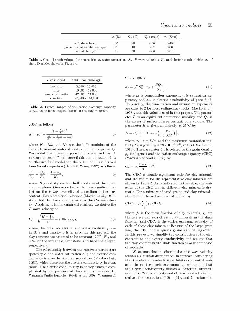
φ (%) Sw (%) Vp (km/s) σe (S/m)
soft shale layer 35 90 2.30 0.430gas saturated sandstone layer 25 10 3.57 0.003
hard shale layer 10 50 4.86 0.018
Table 1. Ground truth values of the porosities φ, water saturations Sw, P -wave velocities Vp, and electric conductivities σe ofthe 1-D model shown in Figure 4.
clay mineral CEC (coulomb/kg)
kaolinite 2,000 - 10,000illite 10,000 - 38,000
montmorillonite 67,000 - 77,000smectite 77,000 - 144,000
Table 2. Typical ranges of the cation exchange capacity(CEC) value for authigenic forms of the clay minerals.
2004) as follows:
K = Kd +(1 − Kd
K0)2
φ
Kf+ 1−φ
K0− Kd
K2
0
, (8)
where Kd, K0, and Kf are the bulk modulus of thedry rock, mineral material, and pore fluid, respectively.We model two phases of pore fluid: water and gas. Amixture of two different pore fluids can be regarded asan effective fluid model and the bulk modulus is derivedfrom Wood’s equation (Batzle & Wang, 1992) as follows:
1
Kf
=Sw
Kw
+1 − Sw
Kg
, (9)
where Kw and Kg are the bulk modulus of the waterand gas phase. One more factor that has significant ef-fect on the P -wave velocity of a medium is the claycontent. Han’s empirical relations (Mavko et al., 1998)state that the clay content c reduces the P -wave veloc-ity. Applying a Han’s empirical relation, we derive theP -wave velocity as
Vp =
s
K + 43µ
ρ− 2.18c km/s, (10)
where the bulk modulus K and shear modulus µ arein GPa and density ρ is in g/cc. In this project, theclay contents are assumed to be constant (20%, 1%, and10% for the soft shale, sandstone, and hard shale layer,respectively).
The relationship between the reservoir parameters(porosity φ and water saturation Sw) and electric con-ductivity is given by Archie’s second law (Mavko et al.,1998), which describes the electric conductivity in cleansands. The electric conductivity in shaley sands is com-plicated by the presence of clays and is described byWaxman-Smits formula (Revil et al., 1998; Waxman &
Smits, 1968):
σe = φmSnw
»
σw +BQv
Sw
–
, (11)
where m is cementation exponent, n is saturation ex-ponent, and σw is electric conductivity of pore fluid.Empirically, the cementation and saturation exponentsare close to 2 for most sedimentary rocks (Mavko et al.,1998), and this value is used in this project. The param-eter B is an equivalent counterion mobility and Qv isthe excess of surface charge per unit pore volume. Theparameter B is given empirically at 25◦C by
B = B0
h
1 − 0.6 exp“
− σw
0.0013
”i
, (12)
where σw is in S/m and the maximum counterion mo-bility B0 is given by 4.78×10⁻⁸ m2/volt/s (Revil et al.,1998). The parameter Qv is related to the grain densityρg (in kg/m3) and the cation exchange capacity (CEC)(Waxman & Smits, 1968) by
Qv = ρg1 − φ
φCEC. (13)
The CEC is usually significant only for clay mineralsand the vaules for the representative clay minerals areshown in Table 2. As is indicated in the table, the vari-ation of the CEC for the different clay mineral is dra-matic. For a mixture of sand grains and clay minerals,the CEC of the sediment is calculated by
CEC = fc
X
i
χi CECi, (14)
where fc is the mass fraction of clay minerals, χi arethe relative fractions of each clay minerals in the shalefraction, and CECi is the cation exchange capacity ofeach of these clay minerals. Because of the large grainsize, the CEC of the quartz grains can be neglected.In this project, we simplify the contribution of the claycontents on the electric conductivity and assume thatthe clay content in the shale fraction is only composedof kaolinite.
We assume that the distribution of P -wave velocityfollows a Gaussian distribution. In contrast, consideringthat the electric conductivity exhibits exponential vari-ation in most geologic environments, we assume thatthe electric conductivity follows a lognormal distribu-tion. The P -wave velocity and electric conductivity arederived from equations (10) - (11), and Gaussian and

56 M.J. Kwon & R. Snieder
Figure 5. Simulated rock-physics model between porosityφ and P -wave velocity Vp. Among three layers, the P -wave
velocity depends least on the porosity in the soft shale layer.
Figure 6. Simulated rock-physics model between water sat-uration Sw and P -wave velocity Vp. The P -wave velocitydepends less on the water saturation than on the porosity.
lognormal random numbers are thereafter added to theP -wave velocity and electric conductivity, respectively,to account for the uncertainty in rock-physics model.Figures 5 through 8 show the simulated rock-physicsmodels, where the porosity and water saturation sam-ples of each layers are retrieved from the prior distribu-tions. The distributions for the P -wave velocity indicatethat the velocity is strongly dependent on the poros-ity and the contribution of the water saturation is lesssignificant. In contrast, the distributions for the elec-tric conductivity show that both the porosity and watersaturation influence the electric conductivity. Note thatthe dependencies are different for each layer. The depen-dency of the P -wave velocity on the porosity is weakestin the soft shale layer and the dependency of the elec-tric conductivity on the water saturation is strongest inthe sandstone layer. These differential dependencies inthe different layers play a significant role in the jointinversion presented in this project.
We assume the likelihoods of the P -wave velocityf(dVp |mφ,mSw ) and logarithm of electric conductiv-ity f(dσe |mφ,mSw) to follow the multivariate Gaus-
Figure 7. Simulated rock-physics model between porosity φ
and electric conductivity σe. For each layer, increased poros-ity tends to accompany larger electric conductivity.
Figure 8. Simulated rock-physics model between water sat-uration Sw and electric conductivity σe. Among three layers,the dependency of the electric conductivity on the water sat-uration is strongest in the sandstone layer.
sian distribution (equation (4)). For the evaluation ofthe likelihoods, we further assume that the P -wave ve-locity and electric conductivity of each layer (Figure 4)to be independent. We model the covariance matricesΣVp and Σσe (Figure 2) as diagonal matrices as shownin equation (5), where the variances σ2
i (Vp) and σ2i (σe)
are constants.
3.2 Seismic data likelihood modeling
There are many kinds of seismic data we can utilize: re-flection data, travel time data, amplitude versus offset orangle data, and full waveform data. The full waveformdata is the most general and encapsulates the largestamount of information. Seismic migration is the mostcommon approach for handling the full waveform datato reconstruct subsurface geometry. The application ofthe full waveform inversion is limited by its poor con-vergence speed.
We use the waveform data for the joint inversionof seismic and CSEM data, because the Monte Carlo

Uncertainty analysis 57
Figure 9. Ray tracing based seismic traces for the 1-D modelshown in Figure 4. The modeled reflection events are gener-ated on the top and bottom boundaries of the gas saturatedsandstone. The central frequency of the source wavelet is 30Hz and the time sampling interval is 3 ms.
method is effective for the least-squares misfit optimiza-tion for the velocities (Jannane et al., 1989; Sniederet al., 1989). Seismic waveform data is synthesized bya ray-tracing algorithm (Docherty, 1987) and we modelthe primary reflections of the P -wave from the top andbottom boundaries of the target sandstone layer. Fig-ure 9 shows the representative time traces simulatedfrom the 1-D model shown in Figure 4. Typical reflec-tion parabola and phase shift at post-critical incidence(Aki & Richards, 2002) are observed. In this project,we use the time series data that corresponds to 2 kmsource-receiver offset and add random noise to the syn-thesized data.
There are many sources of seismic noise in a ma-rine environment: ambient noise, guided waves, tail-buoy noise, shrimp noise, and side-scattered noise (Yil-maz, 1987). We model the seismic noise by adding band-limited noise as shown in Figure 10. The frequency bandof the noise is between 10 and 55 Hz, and the central fre-quency of the source wavelet is 30 Hz. Figure 11 showsa realization of noisy seismic data that is contaminatedby band-limited noise. The maximum amplitude of thenoise is 30% of the maximum amplitude of the noise-freesignal.
We assume that the seismic data likelihood proba-bility f(ds|dVp ) follows the multivariate Gaussian dis-tribution (equation (4)). For the calculation of the like-lihood, it is necessary to evaluate the covariance matrixΣs (Figure 2). For band-limited noise, the covariancematrix follows from the power spectrum of the band-pass filter and the resulting covariance matrix is notdiagonal. We approximate the covariance matrix of aband-limited noise as the covariance matrix of a white
Figure 10. Band-width of the noise (solid line) and am-plitude spectrum of the source wavelet (dashed curve). Theamplitude spectra are normalized for comparison.
Figure 11. Time trace of a data contaminated by the band-limited white noise (solid curve) and noise free data (dashedcurve). The exact P -wave velocities are used for the seismicdata calculation shown here.
noise. We therefore model the covariance matrix as adiagonal matrix as shown in equation (5), where thevariance values σ2
i (ds) are identical.
3.3 CSEM data likelihood modeling
The controlled source electo-magnetic (CSEM) methodhas been studied for the last few decades (Cox et al.,1978) and the feasibility for the delineation of a hy-drocarbon reservoir has recently been discussed (Mehtaet al., 2005). There are several data acquisition geome-tries in the CSEM method and horizontal electric dipoletransmitter and radial electric field response is generallypreferred (Chave & Cox, 1982).
Contrary to seismic wave propagation, EM energytransport within the earth is diffusive and the EM fieldstrength decreases to 1/e order in a length called skindepth (Jackson, 1999), defined as
δ =
r
2
µmσeω≈ 0.503
r
1
σefkm, (15)

58 M.J. Kwon & R. Snieder
Figure 12. Radial electric field amplitude responses for dif-ferent frequencies. Transmitter-receiver offset is 2 km. Tostudy the resoving power of the CSEM method detectingthe target reservoir, the responses from two models are com-pared. The model with reservoir is shown in Figure 4 and themodel without reservoir is comprised of 1.5 km thick seawa-ter, 1.25 km thick soft shale, and hard shale half-space. The
existence of the target sandstone layer is obvious at the highfrequency range.
Figure 13. Two different types of CSEM noise: system-atic noise (open dots) and non-systematic background noise(dashed curve). The systematic noise decreases with fre-quency. In contrast, the non-systematic noise is independentof frequency.
where µm, σe, ω, and f represent magnetic permeability,electric conductivity, angular frequency, and frequency,respectively, all in SI units. For the 1-D model shown inFigure 4, the EM skin depth at 1 Hz is 0.28 km in sea-water, 0.8 km in soft shale, 9.2 km in sandstone, and 3.7km in hard shale layers, respectively. Therefore, about27 % of the EM field passes through the conductiveoverburden and diffuses away through the reservoir.
The CSEM signal measured at a receiver locationis comprised of three components. The first propagatesthrough the solid earth and contains the information onthe reservoir properties. The second propagates throughthe seawater and attenuates rapidly. It is therefore onlysignificant near the transmitter. The third travels as a
Figure 14. Electric field amplitude and phase response of anoise free (solid and dashed curves) and noise contaminatedcase (black and open dots). The exact electric conductivitiesare used for the CSEM data calculation shown here. TheCSEM noise is significant in high frequency range.
wave along the seawater-air interface (air-wave). This isindependent of the earth geology and diminishes withincreasing water depth. In this project, the depth ofthe sea is 1.5 km and the air-wave is not significant.Figure 12 shows the CSEM response for the differ-ent frequencies at 2 km offset. The frequency rangeis from 0.1 to 10 Hz and the CSEM responses fromthe two models are compared each other. The differ-ence between the two models is the existence of sand-stone layer (target reservoir). The existence of the sand-stone layer does not leave an imprint at the low fre-quency range, because the CSEM response at the lowfrequency range is sensitive to the deep electric con-ductivity structure. As we increase the frequency, thediscrepancy between the two CSEM responses becomesmore significant whereas the signal strength becomesweaker. We choose 2 km transmitter-receiver offset andthe frequency range shown in the figure (0.1 ∼ 10 Hz)for further research.
Even though the deep sub-sea environment has lit-tle cultural noise, the CSEM measurements are not en-tirely free from noise. These noise sources include themagneto-telluric signal, streaming potential, and instru-ment noise (Constable & Key, 2007). The magneto-telluric signal is significant at frequencies lower than1 Hz. The streaming potential is generated by seawatermovement. The natural background noise at frequen-cies around 1 Hz is about 1 pV/m (Chave & Cox, 1982)and its influence can be minimized by using a strongertransmitter. The instrument noise is more importantand mainly comes from the transmitter amplifier or re-ceiver electrodes. At lower frequency range, the noisefrom the amplifier and electrodes is proportional to 1/fand 1/
√f , respectively. On the other hand, the instru-
ment noise is saturated at the higher frequency range,i.e., Johnson noise limit (Constable & Key, 2007). Fur-thermore, the CSEM data quality is influenced by posi-tioning error of the transmitter and receiver locations.

Uncertainty analysis 59
Figure 15. Histograms of posterior porosity (φ) samples ofthe sandstone layer. Vertical line indicates the ground truthvalue.
The CSEM data we utilize consists of the real andimaginary parts of the CSEM signal. We design theCSEM noise from the amplitude of the CSEM responseand then add the noise to the real and imaginary partsof the response. The CSEM noise is categorized as sys-tematic and non-systematic noise as shown in Figure 13.The systematic noise includes the instrument noise andthe positioning error. We assume the systematic noiseto be proportional to the amplitude of the CSEM sig-nal whereas the non-systematic noise is independent ofthe signal. A realization of noisy CSEM data is shownin Figure 14, where the systematic noise is 5% of eachnoise-free amplitude and the non-systematic noise is5 × 10−14 V/m. The CSEM signal decreases with fre-quency and the CSEM noise is more obvious.
We assume the CSEM data likelihood probabilityf(de|dσe) to follow the multivariate Gaussian distribu-tion (equation (4)). For the calculation of the likelihood,we assume that the CSEM data noise is independent.We model the covariance matrix Σe (Figure 2) as a di-agonal matrix shown in equation (5). Assuming thatthe systematic and non-systematic noise are uncorre-lated, the diagonal elements of the covariance matrix isderived as
σ2i (de) = σ2
i (εsys) + σ2i (εnonsys), (16)
where εsys and εnonsys denote the systematic and non-systematic noise, respectively. Note that σ2
i (εsys) valuesvary with frequency whereas σ2
i (εnonsys) is independentof frequency.
4 UNCERTAINTY ANALYSIS
4.1 Histogram analysis of posterior
distributions
We perform MCMC sampling to describe the poste-rior probability distribution (equation (3)). The randomsampling is performed within a six dimensional model
Figure 16. Histograms of posterior water saturation (Sw)samples of the sandstone layer. Vertical line indicates theground truth value.
space that accounts for porosity or water saturation ofsoft shale, sandstone, and hard shale layers (Figure 4).The random samples of the porosity and water satura-tion are retrieved from the posterior probability distri-bution of three different cases: using seismic data only,CSEM data only, and both seismic and CSEM data.The uncertainty levels applied to the comparison aresummarized as the base state variances in Table 3. Theposterior distributions of the porosity and water satura-tion of the target sandstone layer are summarized as his-tograms as shown in Figures 15 and 16. Note that for thegiven uncertainties of rock-physics model and data noiselevels, the histograms show that the single interpreta-tions weakly constrain porosity and water saturation.However, the histograms from the joint interpretationexhibit a narrower sample distribution of the porosityand water saturation. The figures also show that theseismic data is more sensitive to the porosity than tothe water saturation. This is connected with the rock-physics models in Figures 5 and 6 which show that theP -wave velocity has weaker correlation with the watersaturation than with porosity. The relatively poor res-olution from the CSEM data is attributed to the factthat the sandstone layer is electrically shielded by themore conductive overburden (soft shale layer). Theseexamples illustrate the strength and limitation of bothseismic and CSEM methods and explain the motivationof the joint interpretation of seismic and CSEM data.The histograms of the joint interpretation show smallerposterior uncertainty than do the single interpretations.The reduction of uncertainty is more pronounced for thewater saturation than for the porosity.
We next compare the histograms that describethe posterior probabilities of different layers. Figure 17shows the joint posterior distributions of the porosity ofthree layers. The posterior distribution for the soft shalelayer is less constrained than that of the other layers.This is a consequence of the relatively weak correlationbetween the porosity and P -wave velocity of the soft

60 M.J. Kwon & R. Snieder
type of uncertainty source base state variance improved state variance
seismic wave velocity (0.1 km/s)2 (0.03 km/s)2
electric conductivity (0.1 log10 (S/m))2 (0.03 log10 (S/m))2
seismic noise (30% of max. amplitude)2 (10% of max. amplitude)2
CSEM noise (systematic) (5% of each amplitude)2 (2% of each amplitude)2
CSEM noise (non-systematic) (5 × 10⁻¹⁴ V/m)2 (2 × 10⁻¹⁴ V/m)2
Table 3. Two representative uncertainty levels used in the project. The base states are the uncertainty levels as shown inFigure 5 - 8, Figure 11, and Figure 14.
Figure 17. Histograms of posterior porosity (φ) samples ofthe three layers obtained from joint inversion of seismic andCSEM data (base uncertainty level). Vertical lines indicatethe ground truth values.
Figure 18. Histograms of posterior water saturation (Sw)samples of the three layers obtained from joint inversion ofseismic and CSEM data (base uncertainty level). Verticallines indicate the ground truth values.
shale layer (Figure 5). Despite the stronger sensitivityof the seismic and CSEM methods on the propertiesof the uppermost layer, the weaker correlations of therock-physics model cause larger variance of the porositysamples. The joint posterior distributions of the watersaturation (Figure 18) also exhibit that the posteriordistribution for the soft shale layer is less constrainedthan for the sandstone layer and that the rock-physics
Figure 19. Histograms of posterior porosity (φ) samplesof the three layers obtained from joint inversion of seismicand CSEM data (improved uncertainty level). Vertical linesindicate the ground truth values.
Figure 20. Histograms of posterior water saturation (Sw)samples of the three layers obtained from joint inversion ofseismic and CSEM data (improved uncertainty level). Verti-cal lines indicate the ground truth values.
model uncertainty has more significance on constrain-ing the posterior distribution than the resolution of theseismic and CSEM methods.
Finally, we study two representative uncertaintylevels: a base state and an improved state (Table 3).Note that the uncertainty of the electric conductivityis defined in logarithmic scale. The seismic data uncer-tainty is defined as a ratio from the maximum ampli-
Uncertainty analysis 61
tude value, and the CSEM data uncertainty is definedas a sum of systematic and non-systematic noise. Fig-ures 17 and 18 represent the posterior probability forthe base uncertainty level. The histograms for the im-proved uncertainty level are shown in Figures 19 and20. The reduced uncertainty level leads, of course, to asharper posterior probability distribution than the basestate and thus enhances the assessment of porosity andwater saturation. This stronger constraint is more obvi-ous for porosity than for water saturation. This is due tothe smaller resolution of the CSEM method comparedto the seismic method.
4.2 Different scenarios for uncertainty
reduction
In the previous section, we presented histograms thatcharacterize the posterior uncertainty. As stated be-fore, we assume the multivariate Gaussian distribution(equation (4)) for the calculation of prior and likelihood.However, there are several factors that make the distri-bution of the posterior samples non-Gaussian. First, theporosity or water saturation have values between 0 and1. Second, the porosity sampling is bounded by the crit-ical porosity φc. The critical porosity is the thresholdvalue between the suspension and the load-bearing do-main and denotes the upper porosity limit of the rangewhere the rock-physics model can be applied (Mavkoet al., 1998). The critical porosity values we apply forthe soft shale, sandstone, and hard shale layer are 0.6,0.4, and 0.4, respectively. These bounds can lead toskewed sample distributions. If the sample distributionsare significantly skewed, another appropriate probabil-ity distribution should be applied for the probabilityassessment of the random samples. In this project, thedistributions of the samples shown in Figure 17 through20 do not display hard bounds or skewed distributionand indicate that the Gaussian distribution is a goodapproximation. The posterior distributions, however, donot necessarily follow the Gaussian distribution becauseof the nonlinearity of the forward models. The posterioruncertainty can generally be assessed by sample meanand sample variance. For reasons of clarity, we use theGaussian curves for the representation of the samplemean and sample variance.
In this project, we model four factors of uncer-tainty: rock-physics model uncertainties of the P -wavevelocity and electric conductivity, and noise of the seis-mic and CSEM data. The posterior probabilities of theporosity and water saturation for the base and improveduncertainty levels (Table 3) are discussed in the previ-ous section (Figures 17 - 20). We perform the followingnumerical experiments to quantify the contributions ofthe four possible sources of uncertainty. The initial sim-ulation is performed based on the base uncertainty level.For the analysis of the contributions of each of the fac-tors on the posterior uncertainties, six subsequent simu-
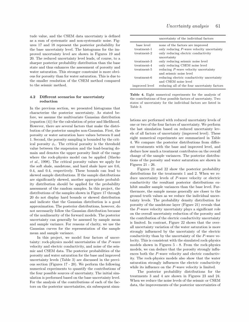
uncertainty of the individual factors
base level none of the factors are improvedtreatment-1 only reducing P -wave velocity uncertaintytreatment-2 only reducing electric conductivity
uncertaintytreatment-3 only reducing seismic noise leveltreatment-4 only reducing CSEM noise leveltreatment-5 reducing P -wave velocity uncertainty
and seismic noise leveltreatment-6 reducing electric conductivity uncertainty
and CSEM noise levelimproved level reducing all of the four uncertainty factors
Table 4. Eight numerical experiments for the analysis ofthe contributions of four possible factors of uncertainty. Two
states of uncertainty for the individual factors are listed inTable 3.
lations are performed with reduced uncertainty levels ofone or two of the four factors of uncertainty. We performthe last simulation based on reduced uncertainty lev-els of all factors of uncertainty (improved level). Theseeight numerical experiments are summarized in Table4. We compare the posterior distributions from differ-ent treatments with the base and improved level, anddeduce how much a treatment contributes on the overallchange of the sample variances. The posterior distribu-tions of the porosity and water saturation are shown inFigures 21 - 26.
Figures 21 and 22 show the posterior probabilitydistributions for the treatments 1 and 2. When we re-duce uncertainty levels of P -wave velocity or electricconductivity the resultant posterior distributions ex-hibit smaller sample variances than the base level. Fur-thermore, the sample means generally are closer to theground truth values as we reduce the individual uncer-tainty levels. The probability density distribution forporosity of the sandstone layer (Figure 21) reveals thatthe P -wave velocity uncertainty plays a significant roleon the overall uncertainty reduction of the porosity andthe contribution of the electric conductivity uncertaintyis limited. In contrast, Figure 22 shows that the over-all uncertainty variation of the water saturation is morestrongly influenced by the uncertainty of the electricconductivity than by the uncertainty of the P -wave ve-locity. This is consistent with the simulated rock-physicsmodels shown in Figures 5 - 8. From the rock-physicsmodels, we can deduce that the porosity strongly influ-ences both the P -wave velocity and electric conductiv-ity. The rock-physics models also show that the watersaturation strongly influences the electric conductivitywhile its influence on the P -wave velocity is limited.
The posterior probability distributions for thetreatments 3 and 4 are shown in Figures 23 and 24.When we reduce the noise levels of the seismic or CSEMdata, the improvements of the posterior uncertainties of

62 M.J. Kwon & R. Snieder
Figure 21. Posterior probability distributions of porosity φ
of the sandstone layer. The distributions from the treatments1 and 2 (Table 4) are compared with those from the baseand improved levels. Vertical line indicates the true porosityvalue.
Figure 22. Posterior probability distributions of water satu-ration Sw of the sandstone layer. The distributions from thetreatments 1 and 2 (Table 4) are compared with those fromthe base and improved levels. Vertical line indicates the truewater saturation value.
the porosity and water saturation are much less signif-icant than the improvements due to the reduction ofrock-physics model uncertainties. This shows that theoverall uncertainty of the porosity and water saturationis more influenced by the rock-physics model uncertain-ties than by the noise of the seismic or CSEM data. Thefigures also show that for the given ranges of data noise,the seismic data noise reduction yields a more preciseestimate than when the CSEM data noise is reduced.
Figures 25 and 26 show the posterior probabilitydistributions for the treatments 5 and 6. Compared tothe single improvement cases, it is clear that the com-bined improvements give better assessments about theporosity and water saturation. The probability densitydistributions shown in Figures 25 and 26 exhibit similardistributions as Figures 21 and 22. This implies that theposterior uncertainty variations from the combined im-provements are mainly governed by the improvement of
Figure 23. Posterior probability distributions of porosity φ
of the sandstone layer. The distributions from the treatments3 and 4 (Table 4) are compared with those from the baseand improved levels. Vertical line indicates the true porosityvalue.
Figure 24. Posterior probability distributions of water satu-ration Sw of the sandstone layer. The distributions from thetreatments 3 and 4 (Table 4) are compared with those fromthe base and improved levels. Vertical line indicates the truewater saturation value.
rock-physics model uncertainties and the contributionsof the seismic and CSEM data noise are less significant.
The posterior probability distributions shown inFigures 21 - 26 are summarized in Table 5. The compar-ison of the variance values clearly show that the reduc-tions of the sample variances of the porosity and watersaturation are most strongly influenced by the uncer-tainty of the P -wave velocity and electric conductiv-ity, respectively. The contributions of the rock-physicsmodel uncertainties on the posterior uncertainties aregenerally larger than those of the seismic and CSEMdata noise. The numerical experiments suggest differentways of accomplishing uncertainty reduction depend-ing on whether our interests focus on the porosity orwater saturation. When the porosity is our prime con-cern, we can effectively accomplish uncertainty reduc-tion by improved rock-physics model about the P -wavevelocity and suppressing the seismic data noise. On theother hand, if we need more accurate assessment about
Uncertainty analysis 63
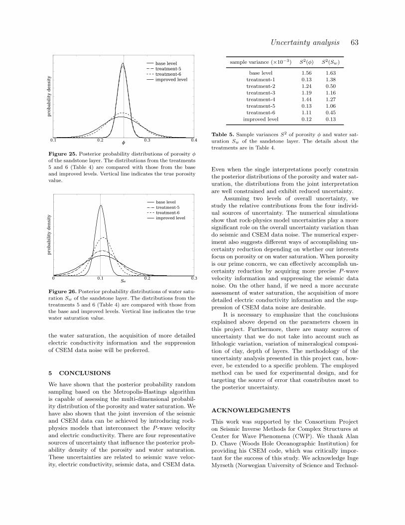
Figure 25. Posterior probability distributions of porosity φ
of the sandstone layer. The distributions from the treatments
5 and 6 (Table 4) are compared with those from the baseand improved levels. Vertical line indicates the true porosityvalue.
Figure 26. Posterior probability distributions of water satu-ration Sw of the sandstone layer. The distributions from thetreatments 5 and 6 (Table 4) are compared with those fromthe base and improved levels. Vertical line indicates the truewater saturation value.
the water saturation, the acquisition of more detailedelectric conductivity information and the suppressionof CSEM data noise will be preferred.
5 CONCLUSIONS
We have shown that the posterior probability randomsampling based on the Metropolis-Hastings algorithmis capable of assessing the multi-dimensional probabil-ity distribution of the porosity and water saturation. Wehave also shown that the joint inversion of the seismicand CSEM data can be achieved by introducing rock-physics models that interconnect the P -wave velocityand electric conductivity. There are four representativesources of uncertainty that influence the posterior prob-ability density of the porosity and water saturation.These uncertainties are related to seismic wave veloc-ity, electric conductivity, seismic data, and CSEM data.
sample variance (×10−3) S2(φ) S2(Sw)
base level 1.56 1.63treatment-1 0.13 1.38treatment-2 1.24 0.50treatment-3 1.19 1.16treatment-4 1.44 1.27treatment-5 0.13 1.06treatment-6 1.11 0.45
improved level 0.12 0.13
Table 5. Sample variances S2 of porosity φ and water sat-uration Sw of the sandstone layer. The details about thetreatments are in Table 4.
Even when the single interpretations poorly constrainthe posterior distributions of the porosity and water sat-uration, the distributions from the joint interpretationare well constrained and exhibit reduced uncertainty.
Assuming two levels of overall uncertainty, westudy the relative contributions from the four individ-ual sources of uncertainty. The numerical simulationsshow that rock-physics model uncertainties play a moresignificant role on the overall uncertainty variation thando seismic and CSEM data noise. The numerical exper-iment also suggests different ways of accomplishing un-certainty reduction depending on whether our interestsfocus on porosity or on water saturation. When porosityis our prime concern, we can effectively accomplish un-certainty reduction by acquiring more precise P -wavevelocity information and suppressing the seismic datanoise. On the other hand, if we need a more accurateassessment of water saturation, the acquisition of moredetailed electric conductivity information and the sup-pression of CSEM data noise are desirable.
It is necessary to emphasize that the conclusionsexplained above depend on the parameters chosen inthis project. Furthermore, there are many sources ofuncertainty that we do not take into account such aslithologic variation, variation of mineralogical composi-tion of clay, depth of layers. The methodology of theuncertainty analysis presented in this project can, how-ever, be extended to a specific problem. The employedmethod can be used for experimental design, and fortargeting the source of error that constributes most tothe posterior uncertainty.
ACKNOWLEDGMENTS
This work was supported by the Consortium Projecton Seismic Inverse Methods for Complex Structures atCenter for Wave Phenomena (CWP). We thank AlanD. Chave (Woods Hole Oceanographic Institution) forproviding his CSEM code, which was critically impor-tant for the success of this study. We acknowledge IngeMyrseth (Norwegian University of Science and Technol-

64 M.J. Kwon & R. Snieder
ogy), Malcolm Sambridge (Australian National Univer-sity), Albert Tarantola (Institut de Physique du Globede Paris), Luis Tenorio, Mike Batzle, Andre Revil, MisacNabighian, Steve Hill (Colorado School of Mines) forhelpful information, discussions, and suggestions. Weare also grateful to colleagues of CWP for valuable dis-cussions and technical help.
REFERENCES
Aki, K., & Richards, P. G. 2002. Quantitative Seismology.2nd edn. University Science Books.
Batzle, M., & Wang, Z. 1992. Seismic properties of porefluids. Geophysics, 57, 1396 – 1408.
Chave, A., & Cox, C. S. 1982. Controlled ElectromagneticSources for Measuring Electrical Conductivity Beneaththe Oceans 1. Forward Problem and Model Study. Jour-
nal of Geophysical Research, 87, 5327 – 5338.Chen, J., Hoversten, G. M., Vasco, D., Rubin, Y., & Hou,
Z. 2007. A Bayesian model for gas saturation estimationusing marine seismic AVA and CSEM data. Geophysics,72, WA85 – WA95.
Constable, S., & Key, K. 2007. Marine Electromagnetic
Methods for Hydrocarbon Exploration. Sociey of Explo-ration Geophysics.
Cox, C. S., Kroll, N., Pistek, P., & Watson, K. 1978. Electro-magnetic Fluctuations Induced by Wind Waves on theDeep-Sea Floor. Journal of Geophysical Research, 83,431 – 442.
Docherty, P. 1987. Ray theoretical modeling, migration
and inversion in two-and-one-half-dimensional layered
acoustic media. Ph.D. dissertation. Colorado School ofMines.
Gallardo, L. A., & Meju, M. A. 2004. Joint two-dimensionalDC resistivity and seismic travel time inversion withcross-gradients constraints. Journal of Geophysical Re-
search, 109, B03311.Geman, S., & Geman, D. 1984. Stochastic Relaxation, Gibbs
distribution, and the Bayesian Restoration of Images.IEEE Trans on Pattern Analysis and Machine Intelli-
gence, 6, 721 – 741.Gouveia, W. P., & Scales, J. A. 1998. Bayesian seismic wave-
form inversion: Parameter estimation and uncertaintyanalysis. Journal of Geophysical Research, 103, 2759– 2779.
Han, D., & Batzle, M. 2004. Gassmann’s equation and fluid-saturation effects on seismic velocities. Geophysics, 69,398 – 405.
Harris, P., & MacGregor, L. 2006. Determination of reservoirproperties from the integration of CSEM, seismic, andwell-log data. First Break, 24, 53 – 59.
Hastings, W. K. 1970. Monte Carlo sampling methods usingMarkov chains and their applications. Biometrika, 57,97 – 109.
Hoversten, G. M., Cassassuce, F., Gasperikova, E., Newman,G. A., Chen, J., Rubin, Y., Hou, Z., & Vasco, D. 2006.Direct reservoir parameter estimation using joint inver-sion of marine seismic AVA and CSEM data. Geophysics,71, C1 – C13.
Jackson, J. D. 1999. Classical Electrodynamics. 3rd edn.John Wiley & Sons.
Jannane, M., Beydoun, W., Crase, E., Cao, D., Koren, Z.,
Landa, E., Mendes, M., Pica, A., Noble, M., Roeth, G.,Singh, S., Snieder, S., Tarantola, A., Trezeguet, D., &Xie, M. 1989. Wavelengths of earth structures that canbe resolved from seismic reflection data. Geophysics, 54,906 – 910.
Kaipio, J. P., Kolehmainen, V., Somersalo, E., & Vauhkonen,M. 2000. Statistical inversion and monte Carlo samplingmethods in electrical impedance tomography. Inverse
Problems, 16, 1487 – 1522.Mavko, G., Mukerji, T., & Dvorkin, J. 1998. The Rock
Physics Handbook. Cambridge University Press.Mehta, K., Nabighian, M. N., Li, Y., & Oldenburg, D. W.
2005. Controlled Source Electromagnetic (CSEM) tech-nique for detection and delineation of hydrocarbon reser-voirs: an evaluation. SEG Expanded Abstract, 75, 546 –549.
Metropolis, N., Rosenbluth, A. W., Rosenbluth, M. N., &Teller, A. H. 1953. Equation of State Calculations by FastComputing Machines. The Journal of Chemical Physics,21, 1087 – 1092.
Mosegaard, K., & Sambridge, M. 2002. Monte Carlo analysisof inverse problems. Inverse Problems, 18, R29 – R54.
Mosegaard, K., Singh, S., Snyder, D., & Wagner, H. 1997.Monte Carlo analysis of seismic reflections from Mohoand the W reflector. Journal of Geophysical Research,102, 2969 – 2981.
Musil, M., Maurer, H. R., & Green, A. G. 2003. Discretetomography and joint inversion for loosely connected orunconnected physical properties: application to crossholeseismic and georadar data sets. Geophysical Journal In-
ternational, 153, 389 – 402.Revil, A., Cathles, L. M., & Losh, S. 1998. Electrical con-
ductivity in shaly sands with geophysical applications.Journal of Geophysical Research, 103, 23925 – 23936.
Sambridge, M., Beghein, C., Simons, F. J., & Snieder, R.2006. How do we understand and visualize uncertainty?Leading Edge, 25, 542 – 546.
Scales, J. A., & Snieder, R. 1997. To Bayes or not to Bayes?Geophysics, 62, 1045 – 1046.
Scales, J. A., & Tenorio, L. 2001. Prior information anduncertainty in inverse problems. Geophysics, 66, 389 –397.
Sivia, D. S., & Webster, J. R. P. 1998. The Bayesian approachto reflectivity data. Physica B, 248, 327 – 337.
Snieder, R. 1998. The role of nonlinearity in inverse prob-lems. Inverse Problems, 14, 387 – 404.
Snieder, R., Xie, M. Y., Pica, A., & Tarantola, A. 1989. Re-trieving both the impedance contrast and backgroundvelocity: A global strategy for the seismic reflection prob-lem. Geophysics, 54, 991 – 1000.
Spikes, K., Mukerji, T., Dvorkin, J., & Mavko, G. 2007. Prob-abilistic seismic inversion based on rock-physics models.Geophysics, 72, R87 – R97.
Tenorio, L. 2001. Statistical Regularization of Inverse Prob-lems. SIAM Review, 43, 347 – 366.
Waxman, M. H., & Smits, L. J. M. 1968. Electrical conduc-tivities in oil-bearing shaly sands. Society of Petroleum
Engineering Journal, 8, 107 – 122.Yilmaz, O. 1987. Seismic Data Processing. Sociey of Explo-
ration Geophysics.