Ultrasound Imaging

Ho Kyung Kim

Pusan National University

Introduction to Medical Engineering (Medical Imaging)

Suetens 6

• Sound

– Sonic: 20 Hz–20 kHz (audible frequency)

– Subsonic (<) and ultrasonic (>)

• Ultrasound

– Acoustic wave

– Reflects, diffracts, refracts, attenuates, disperses, and scatters when it propagates through matter

• Ultrasound imaging

– Estimates the tissue position by measuring the travel time of ultrasound that reflects at the

interface between different tissues (with the known acoustic wave velocity)

– Noninvasive, inexpensive, portable

– Excellent temporal resolution

– Being applied to nondestructive testing (NDT) and sound navigation ranging (SONAR)

– Not only to visualize morphology or anatomy but also to visualize function by means of blood and

myocardial velocities (velocity imaging ⇒ Doppler imaging)

2

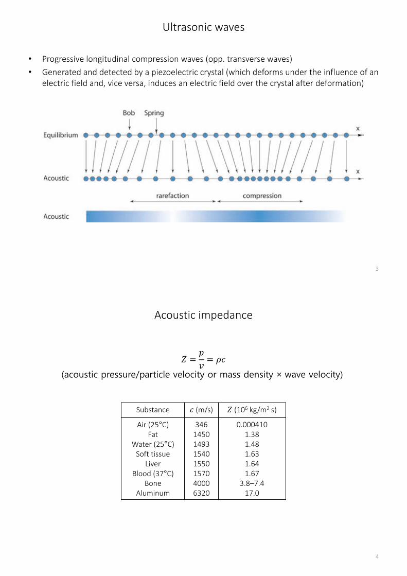
Ultrasonic waves

• Progressive longitudinal compression waves (opp. transverse waves)

• Generated and detected by a piezoelectric crystal (which deforms under the influence of an

electric field and, vice versa, induces an electric field over the crystal after deformation)

3

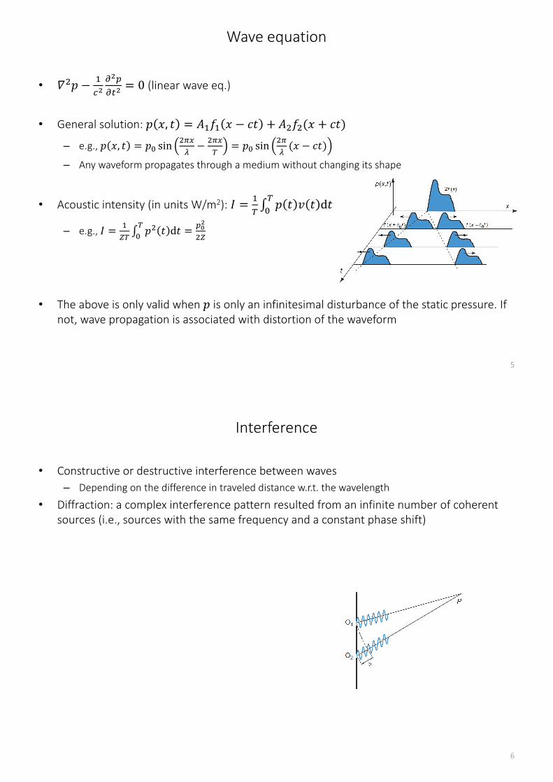
Acoustic impedance

Substance � (m/s) � (106 kg/m2 s)

Air (25°C)

Fat

Water (25°C)

Soft tissue

Liver

Blood (37°C)

Bone

Aluminum

346

1450

1493

1540

1550

1570

4000

6320

0.000410

1.38

1.48

1.63

1.64

1.67

3.8–7.4

17.0

4

� =�

�= ��

(acoustic pressure/particle velocity or mass density × wave velocity)

Wave equation

• ��� −

�� ��

��= 0 (linear wave eq.)

• General solution: � �, � = �� � − �� + ����(� + ��)

– e.g., � �, � = �� sin���

�−

���

= �� sin

��

�(� − ��)

– Any waveform propagates through a medium without changing its shape

• Acoustic intensity (in units W/m2): ! =

" � � � � d�

�

– e.g., ! =

$ " �� � d�

�=

�%�

�$

• The above is only valid when � is only an infinitesimal disturbance of the static pressure. If

not, wave propagation is associated with distortion of the waveform

5

Interference

• Constructive or destructive interference between waves

– Depending on the difference in traveled distance w.r.t. the wavelength

• Diffraction: a complex interference pattern resulted from an infinite number of coherent

sources (i.e., sources with the same frequency and a constant phase shift)

6

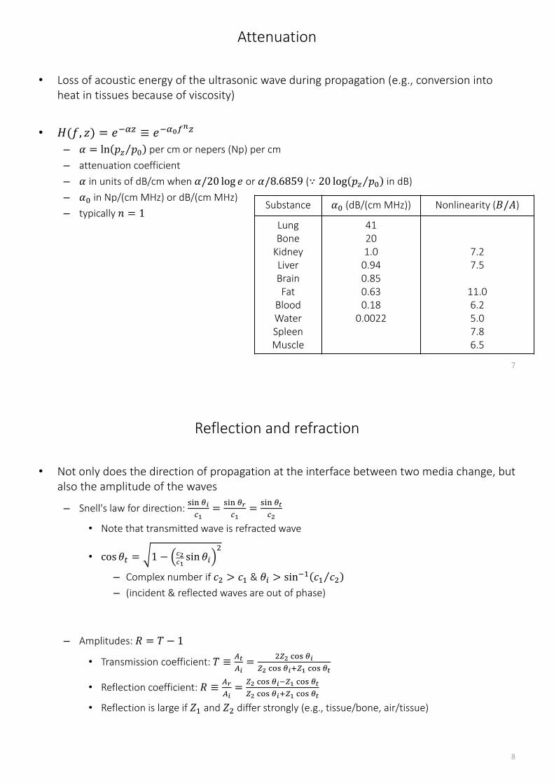
Attenuation

• Loss of acoustic energy of the ultrasonic wave during propagation (e.g., conversion into

heat in tissues because of viscosity)

• &(�, ') = ()*+ ≡ ()*%-.+

– / = ln �+ ��⁄ per cm or nepers (Np) per cm

– attenuation coefficient

– / in units of dB/cm when //20 log ( or //8.6859 (∵ 20 log �+ ��⁄ in dB)

– /� in Np/(cm MHz) or dB/(cm MHz)

– typically < = 1

7

Substance /� (dB/(cm MHz)) Nonlinearity (>/�)

Lung

Bone

Kidney

Liver

Brain

Fat

Blood

Water

Spleen

Muscle

41

20

1.0

0.94

0.85

0.63

0.18

0.0022

7.2

7.5

11.0

6.2

5.0

7.8

6.5

Reflection and refraction

• Not only does the direction of propagation at the interface between two media change, but

also the amplitude of the waves

– Snell's law for direction: ?@A BC�D

=?@A BE�D

=?@A BF��

• Note that transmitted wave is refracted wave

• cos H� = 1 − I�IDsin HJ

�

– Complex number if �� > � & HJ > sin) � ��⁄

– (incident & reflected waves are out of phase)

– Amplitudes: L = M − 1

• Transmission coefficient: M ≡NFNC=

�$� OP? BC$� OP? BCQ$D OP? BF

• Reflection coefficient: L ≡NENC=

$� OP? BC)$D OP? BF$� OP? BCQ$D OP? BF

• Reflection is large if � and �� differ strongly (e.g., tissue/bone, air/tissue)

8

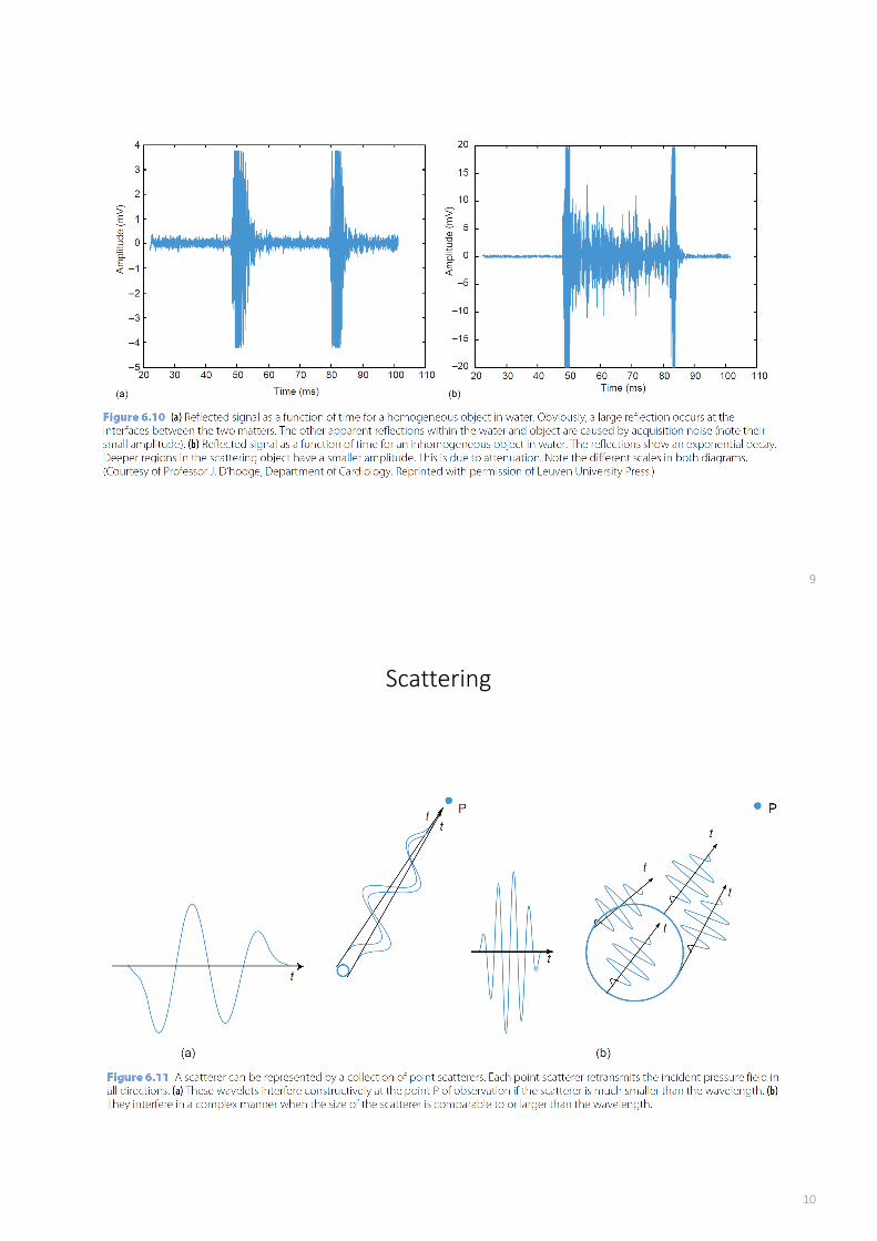
9

Scattering

10

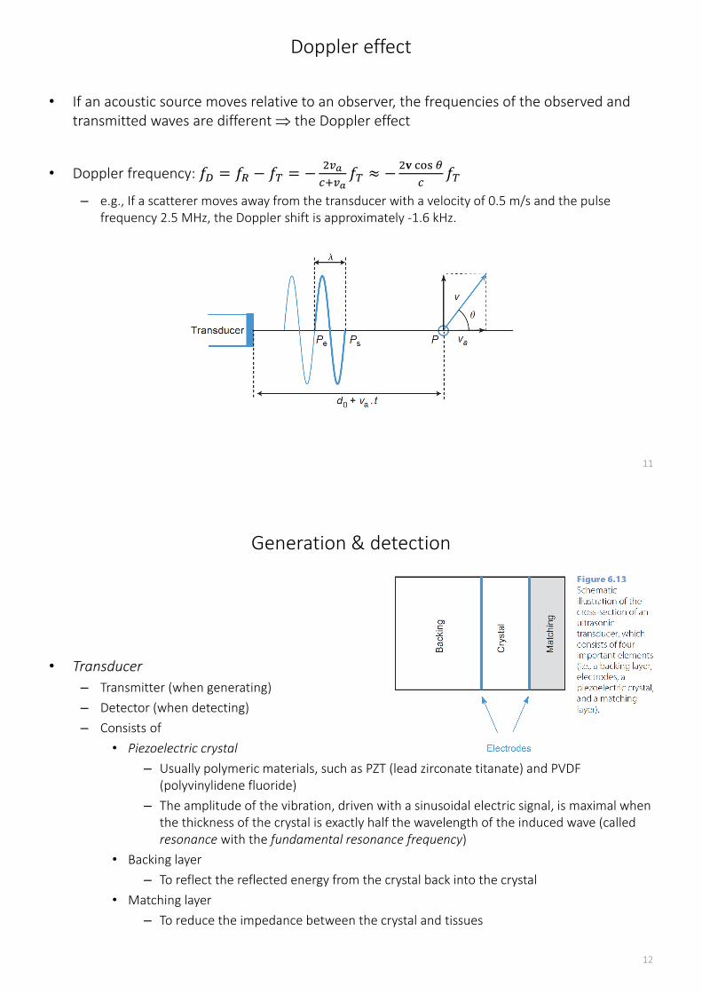
Doppler effect

• If an acoustic source moves relative to an observer, the frequencies of the observed and

transmitted waves are different ⇒ the Doppler effect

• Doppler frequency: �R = �S − � = −�TU�QTU

� ≈ −�W OP? B

��

– e.g., If a scatterer moves away from the transducer with a velocity of 0.5 m/s and the pulse

frequency 2.5 MHz, the Doppler shift is approximately -1.6 kHz.

11

Generation & detection

• Transducer

– Transmitter (when generating)

– Detector (when detecting)

– Consists of

• Piezoelectric crystal

– Usually polymeric materials, such as PZT (lead zirconate titanate) and PVDF

(polyvinylidene fluoride)

– The amplitude of the vibration, driven with a sinusoidal electric signal, is maximal when

the thickness of the crystal is exactly half the wavelength of the induced wave (called

resonance with the fundamental resonance frequency)

• Backing layer

– To reflect the reflected energy from the crystal back into the crystal

• Matching layer

– To reduce the impedance between the crystal and tissues

12

Gray-scale imaging

• A-mode (amplitude) imaging

– Based on the pulse-echo principle

– Measurements of the reflected waves as a function of time

• X =�×∆�

�

– Detected signal ~ MHz range (∴ called RF signal)

• M-mode (motion) imaging

– Repeated A-mode measurements for a moving object

13

• B-mode (brightness) imaging

– Repeated A-mode measurements by translating or tilting the transducer

14

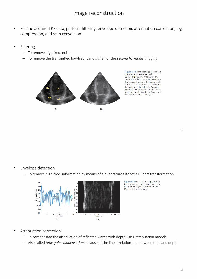
Image reconstruction

• For the acquired RF data, perform filtering, envelope detection, attenuation correction, log-

compression, and scan conversion

• Filtering

– To remove high-freq. noise

– To remove the transmitted low-freq. band signal for the second harmonic imaging

15

• Envelope detection

– To remove high-freq. information by means of a quadrature filter of a Hilbert transformation

16

• Attenuation correction

– To compensate the attenuation of reflected waves with depth using attenuation models

– Also called time gain compensation because of the linear relationship between time and depth

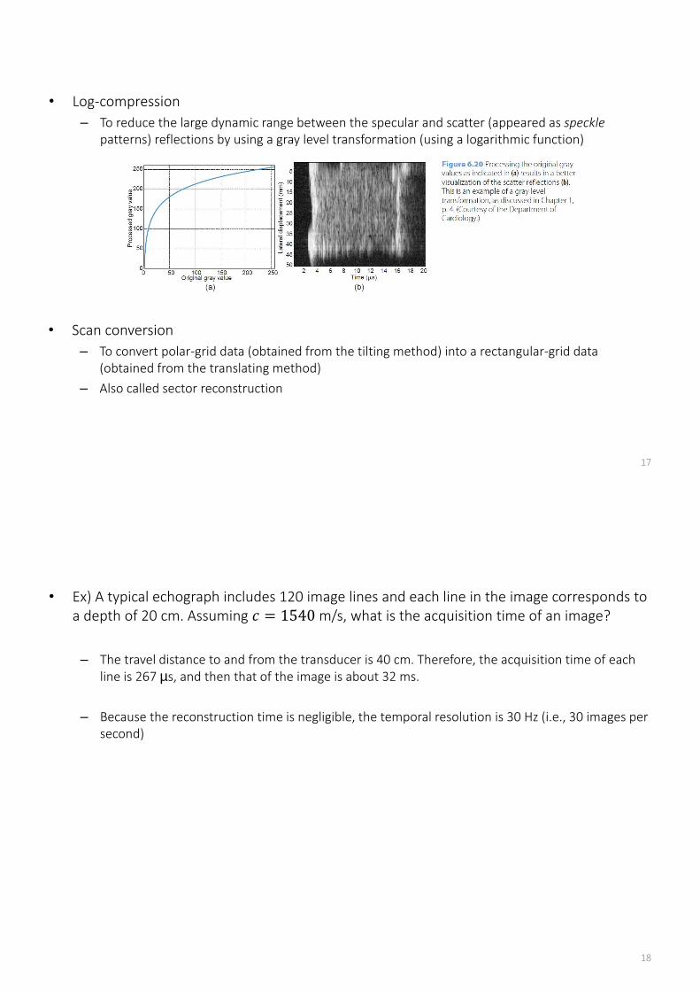
• Log-compression

– To reduce the large dynamic range between the specular and scatter (appeared as speckle

patterns) reflections by using a gray level transformation (using a logarithmic function)

17

• Scan conversion

– To convert polar-grid data (obtained from the tilting method) into a rectangular-grid data

(obtained from the translating method)

– Also called sector reconstruction

• Ex) A typical echograph includes 120 image lines and each line in the image corresponds to

a depth of 20 cm. Assuming � = 1540 m/s, what is the acquisition time of an image?

– The travel distance to and from the transducer is 40 cm. Therefore, the acquisition time of each

line is 267 µs, and then that of the image is about 32 ms.

– Because the reconstruction time is negligible, the temporal resolution is 30 Hz (i.e., 30 images per

second)

18

Doppler imaging

• To visualize velocities of moving tissues

• 3 different data acquisition methods

1) Continuous wave (CW) Doppler

• Two crystal for transmitting continuous sinusoidal wave and detecting in the same

transducer

• Only exception to the pulse-echo principle

• No spatial (i.e., depth) information

2) Pulsed wave (PW) Doppler

• Transmitting pulsed waves at a constant pulse repetition frequency (PRF)

• M-mode acquisition but only one sample per each line at a fixed time (i.e., range gate),

resulting in one specific spatial position

3) Color flow (CF) imaging

• B-mode acquisition but, for each image line, several pulses (3–7) instead of one are

transmitted

• 2D anatomical gray scale image onto where the color velocity information is superimposed

19

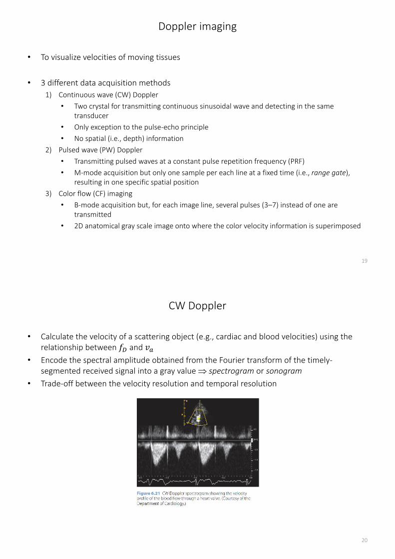
CW Doppler

• Calculate the velocity of a scattering object (e.g., cardiac and blood velocities) using the

relationship between �R and �^• Encode the spectral amplitude obtained from the Fourier transform of the timely-

segmented received signal into a gray value ⇒ spectrogram or sonogram

• Trade-off between the velocity resolution and temporal resolution

20

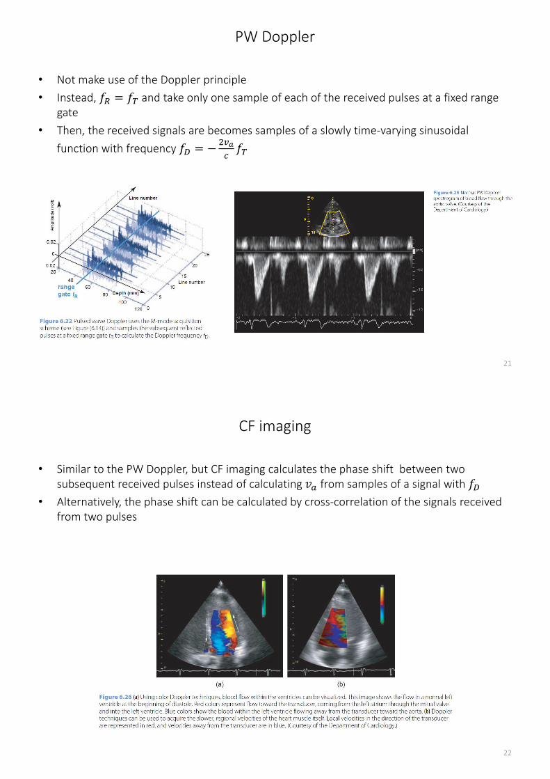
PW Doppler

• Not make use of the Doppler principle

• Instead, �S = � and take only one sample of each of the received pulses at a fixed range

gate

• Then, the received signals are becomes samples of a slowly time-varying sinusoidal

function with frequency �R = −�TU��

21

CF imaging

• Similar to the PW Doppler, but CF imaging calculates the phase shift between two

subsequent received pulses instead of calculating �^ from samples of a signal with �R• Alternatively, the phase shift can be calculated by cross-correlation of the signals received

from two pulses

22

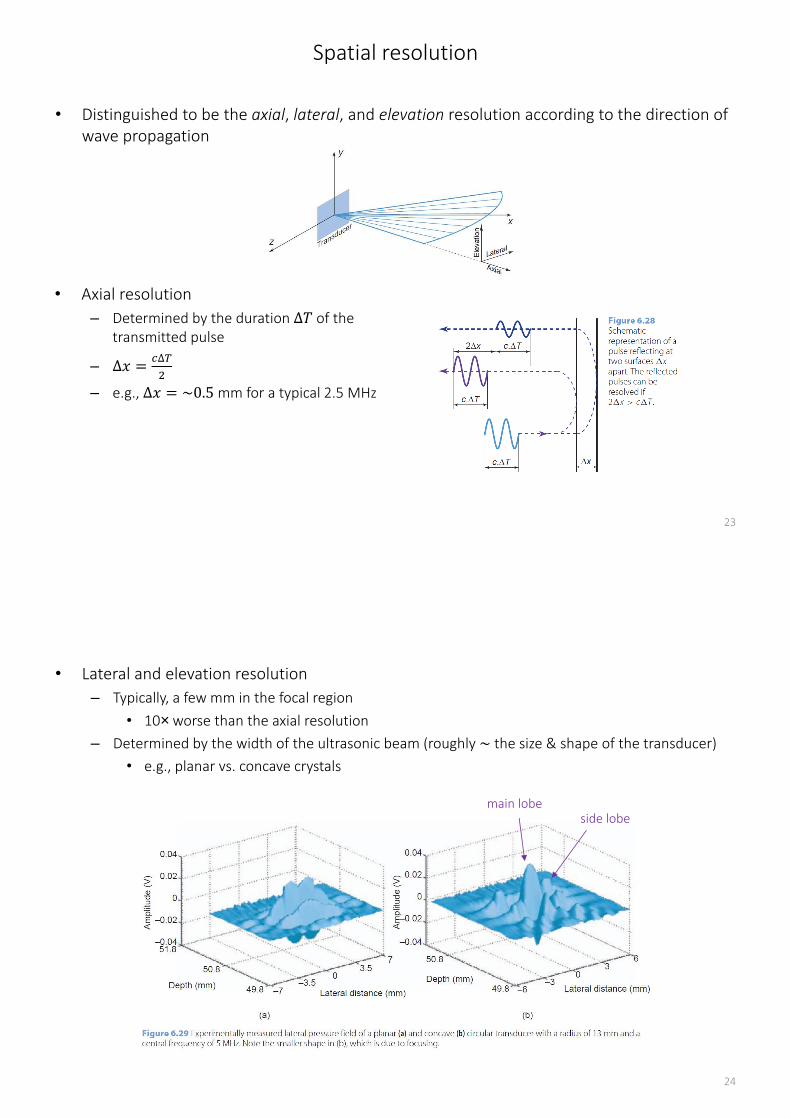
Spatial resolution

• Distinguished to be the axial, lateral, and elevation resolution according to the direction of

wave propagation

23

• Axial resolution

– Determined by the duration ∆M of the

transmitted pulse

– ∆� =�∆

�

– e.g., ∆� = ~0.5 mm for a typical 2.5 MHz

• Lateral and elevation resolution

– Typically, a few mm in the focal region

• 10× worse than the axial resolution

– Determined by the width of the ultrasonic beam (roughly ~ the size & shape of the transducer)

• e.g., planar vs. concave crystals

24

main lobeside lobe

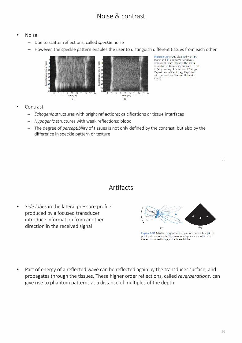
Noise & contrast

• Noise

– Due to scatter reflections, called speckle noise

– However, the speckle pattern enables the user to distinguish different tissues from each other

25

• Contrast

– Echogenic structures with bright reflections: calcifications or tissue interfaces

– Hypogenic structures with weak reflections: blood

– The degree of perceptibility of tissues is not only defined by the contrast, but also by the

difference in speckle pattern or texture

Artifacts

• Side lobes in the lateral pressure profile

produced by a focused transducer

introduce information from another

direction in the received signal

26

• Part of energy of a reflected wave can be reflected again by the transducer surface, and

propagates through the tissues. These higher order reflections, called reverberations, can

give rise to phantom patterns at a distance of multiples of the depth.

27

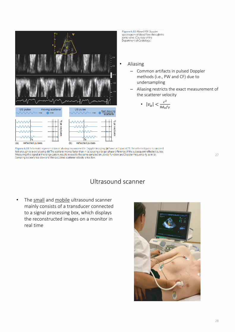
• Aliasing

– Common artifacts in pulsed Doppler

methods (i.e., PW and CF) due to

undersampling

– Aliasing restricts the exact measurement of

the scatterer velocity

• �^ <��

`a%-b

Ultrasound scanner

• The small and mobile ultrasound scanner

mainly consists of a transducer connected

to a signal processing box, which displays

the reconstructed images on a monitor in

real time

28

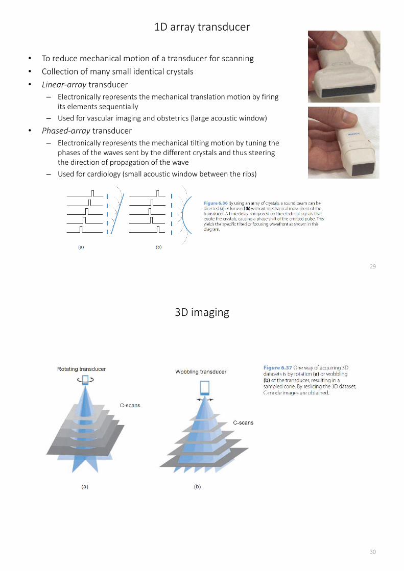
1D array transducer

• To reduce mechanical motion of a transducer for scanning

• Collection of many small identical crystals

• Linear-array transducer

– Electronically represents the mechanical translation motion by firing

its elements sequentially

– Used for vascular imaging and obstetrics (large acoustic window)

• Phased-array transducer

– Electronically represents the mechanical tilting motion by tuning the

phases of the waves sent by the different crystals and thus steering

the direction of propagation of the wave

– Used for cardiology (small acoustic window between the ribs)

29

3D imaging

30

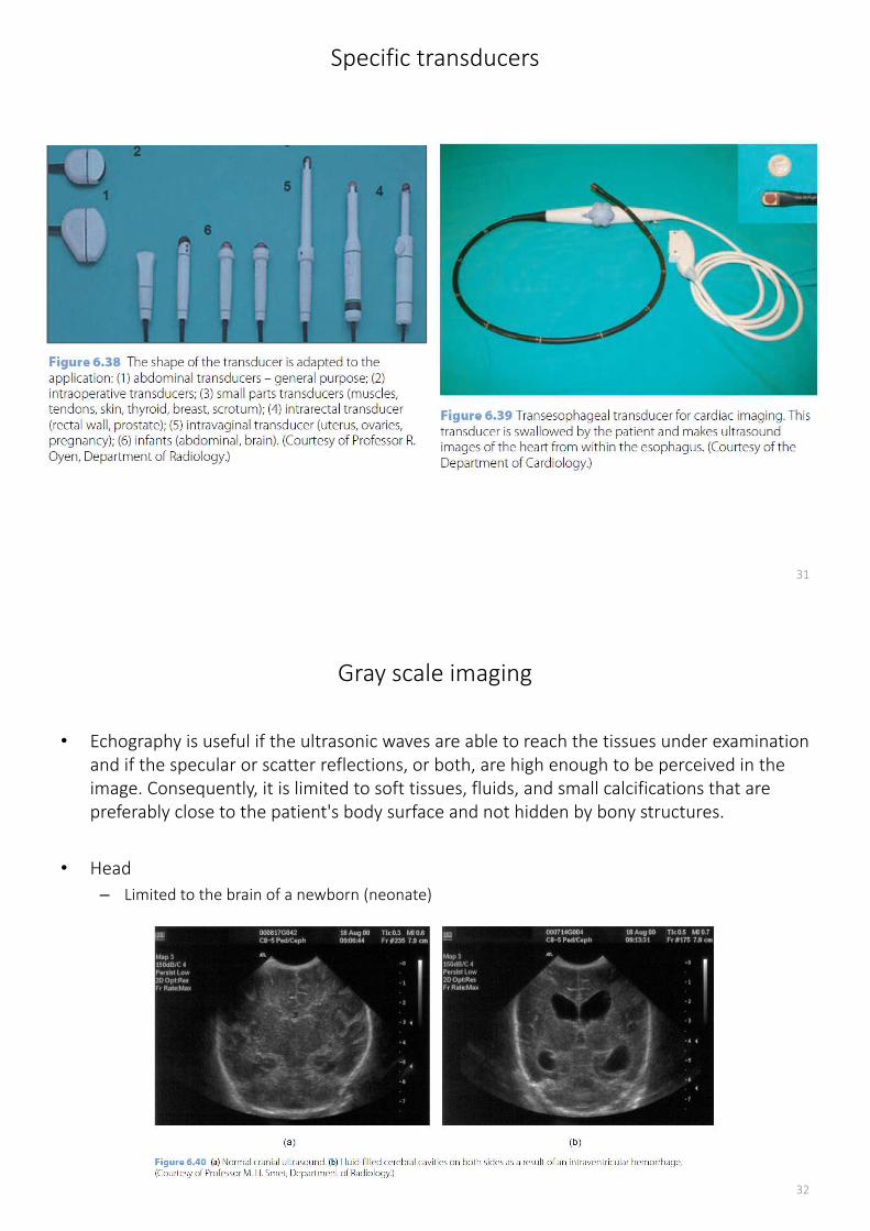
Specific transducers

31

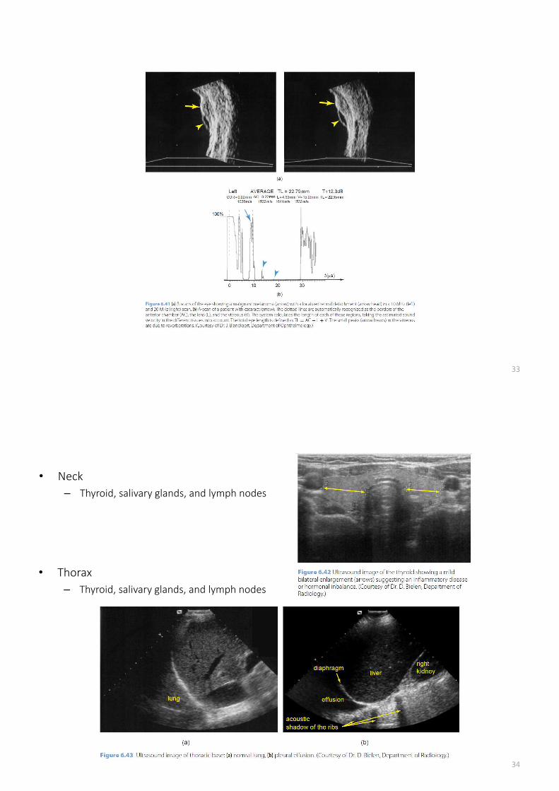
Gray scale imaging

• Echography is useful if the ultrasonic waves are able to reach the tissues under examination

and if the specular or scatter reflections, or both, are high enough to be perceived in the

image. Consequently, it is limited to soft tissues, fluids, and small calcifications that are

preferably close to the patient's body surface and not hidden by bony structures.

• Head

– Limited to the brain of a newborn (neonate)

32

33

• Neck

– Thyroid, salivary glands, and lymph nodes

34

• Thorax

– Thyroid, salivary glands, and lymph nodes

• Breast

– Mostly combined with mammography for

differential diagnosis

35

• Fetus, uterus, and placenta

36

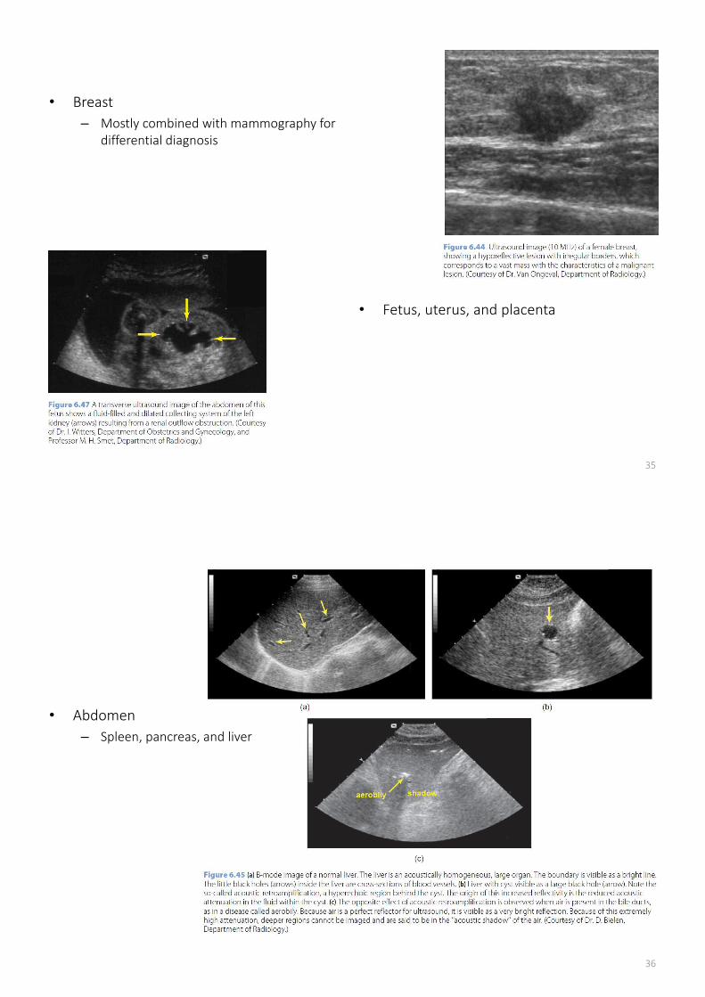
• Abdomen

– Spleen, pancreas, and liver

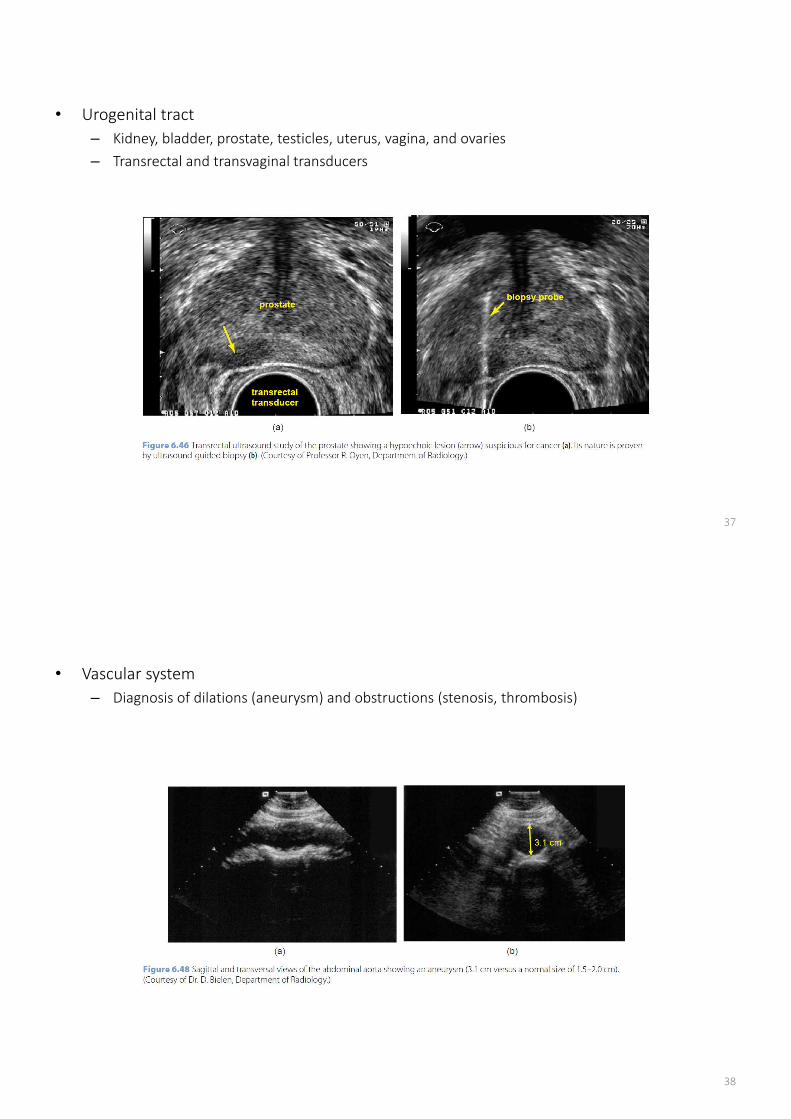
• Urogenital tract

– Kidney, bladder, prostate, testicles, uterus, vagina, and ovaries

– Transrectal and transvaginal transducers

37

• Vascular system

– Diagnosis of dilations (aneurysm) and obstructions (stenosis, thrombosis)

38

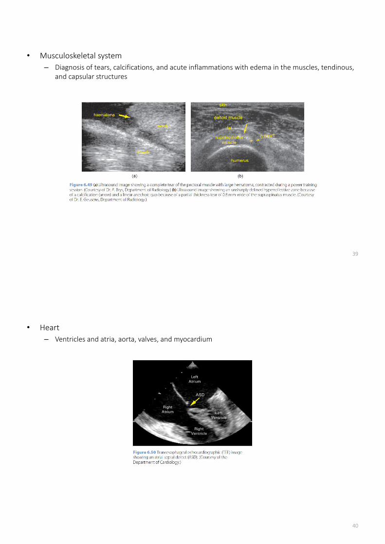
• Musculoskeletal system

– Diagnosis of tears, calcifications, and acute inflammations with edema in the muscles, tendinous,

and capsular structures

39

• Heart

– Ventricles and atria, aorta, valves, and myocardium

40

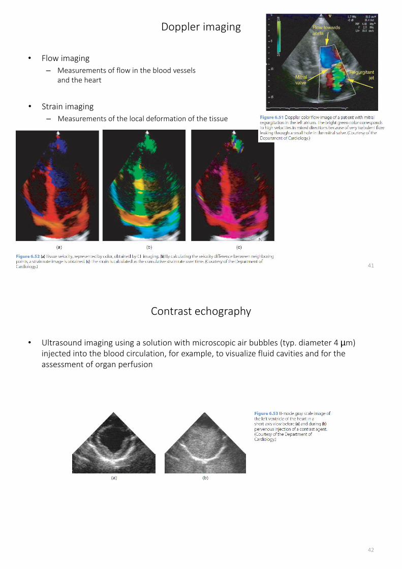
Doppler imaging

• Flow imaging

– Measurements of flow in the blood vessels

and the heart

41

• Strain imaging

– Measurements of the local deformation of the tissue

Contrast echography

• Ultrasound imaging using a solution with microscopic air bubbles (typ. diameter 4 µm)

injected into the blood circulation, for example, to visualize fluid cavities and for the

assessment of organ perfusion

42

Biological effects and safety

• Tissue heating

– Tissue damage due to heat converted from ultrasonic energy

– Monitor the thermal index based on the transmitted power not to exceed a certain threshold

– Heating can be used for ultrasound surgery to burn malignant tissue

• Cavitation

– Tissue damage due to the collapse of bubbles that are formed in areas of low local density

resulting from a negative pressure

– Monitor the mechanical index based on the peak negative pressure not to exceed a certain

threshold

– Cavitation is the basis for lithogripsers, which destroy kidney or bladder stones by means of high-

pressure ultrasound

43