Ultra Short Tenor Yield Curves For

High-Frequency Trading and Blockchain

Settlement

Anton Golub, Lidan Grossmass, and Ser-Huang Poon∗

March 2, 2018

∗Anton Golub (anton.golub@lykke.com) is the co-founder of Lykke Corp, Zurich, Switzerland; Li-

dan Grossmass (lidan.grossmass@hhu.de) is at the Department of Economics, University of Dussel-

dorf, Germany; Ser Huang Poon (ser-huang.poon@mancheter.ac.uk) is at the Alliance Manchester Busi-

ness School, University of Manchester, UK. The funding from Manchester University FinTech Initiative

2017 is gratefully acknowledged. We would also like to thank the participants of the Shanghai FinTech

Conference 2017, AMBS seminar, Eduardo Salazar and Michael Brennan for helpful comments in writ-

ing this paper.

Ultra Short Tenor Yield Curve For

High-Frequency Trading and Blockchain

Settlement

Abstract

Blockchain, based on the distributed ledger technology, provides immediate set-

tlement of transactions of digital assets and direct ownership. Since settlement of

transactions is immediate, the blockchain system requires an ultra short tenor in-

terest rate curve that is always up-to-date. Today, many market-quoted rates are

still accrued at the end of each trading day, typically with one day as the shortest

tenor available. This paper develops an interbank money market model for the

equilibrium interest rate of ultra short tenor and updated at an intraday level with

automated adjustment for the event of a flash crash. Apart from facilitating trades

settlement on blockchain, our research findings are vital for central banks’ efforts

in stabilizing the currencies during flash crashes. We show that during the flash

crash on 15 January 2015 when the Swiss National Bank (SNB) dropped the floor

of CHF 1.2 per EUR, the ultra short CHF interest rates should have been highly

negative to incentivize market makers to provide liquidity during the sharp CHF

appreciation and to neutralize the arbitrage activities that aggravated the crash.

JEL-Classification: G01, G12, G14, G23, C01, C15, C41, C58

Keywords: Blockchain, Intraday Yield Curve, Flash Crash, Duration and Time De-

formation

2

1 Introduction

Flash crashes are typically short-lived but have the potential to undermine confi-

dence in financial markets. Trading today occurs at high speed with traders opening

and closing positions in rapid succession and it is estimated that more than 90% of

currency positions are held for less than 24 hours, and typically only for minutes or

a few hours (Golub et al. (2013)). If only the overnight positions attract interest rate

charges, this means that in practice only a small portion of FX transactions actually

triggers interest payments. In the event of a large intraday selling pressure of a partic-

ular currency, the central bank is helpless against this type of ’flash crash’ (Kirilenko

et al. (2014)), which can potentially lead to permanent economic losses.

Central banks can intervene in financial markets to stabilize their currencies by

buying or selling foreign currency reserves but that often comes at a cost of rapid

expansion or shrinkage of their balance sheets, as well as disruptions in financial

markets and the real economy. Until 2015, the Swiss National Bank (SNB) has ac-

cumulated over 500 billion CHF worth of currency reserves by maintaining a floor on

EUR/CHF, but only to see the market value of those reserves drop by over 60 billion

CHF in a matter of hours when the floor was abandoned on 15 January 2015. In ex-

treme situations, the central bank can drastically change short-term interest rates as

a measure of last resort to protect its currency. Without the ultra short tenor rates,

the central bank can only change the overnight 1-day rate or the base rate. Using the

1-day rate to manage ultra high frequency trading and to counteract flash crashes can

cause disruptions to the financial system and the real economy. In another instance, in

2000 the Turkish Central Bank had to raise daily interest rates to 300% at the height of

the crisis to prevent the currency from collapsing, driving many banks and corpora-

tions into bankruptcy and resulting in over 1 million people losing their jobs (Özatay

(2002)). Today, Brexit and the instability of world political situations are the type of

market conditions that germinate currency volatility, often in the ultra-high frequency

3

space.

Blockchain, or distributed ledger technology, is an infrastructure that allows for

immediate settlement.1 Traditional ways of clearing and settling trades based on cen-

tralized ledgers require batch-based serial processes that often result in multi-day set-

tlement times, along with high costs and operational risks. Since blockchain allows

for immediate settlement of transaction,2 it will pave the way for the development

of the ultra short tenor interest rate market. The yield curve will start with, for ex-

ample, a one-second duration instead of one day, as is currently the case, and extend

outward and converge to the 1-day rate as the tenor approaches 86,400 seconds. An

important effect of fast clearing and settlement is the reduction in costs, counterparty

and liquidity risks. In essence, the blockchain is a universally accessible ledger and a

decentralized notary service that ensures global consensus on completed transactions

and asset ownership. Like the world wide web, the ledger is not controlled by a single

entity but by all market participants. The ’global’ nature of the blockchain allows it to

extend beyond country borders, central bank regulations, traditional trading hours,

and exchanges. This emergent technology has revolutionized the way financial mar-

kets work and more structural changes are to be expected.

The key concerns of policy makers are that systemic financial institutions are not

undermined, market is resilient, and that flash events should ideally not happen nor

produce systemic contagion across markets. However the fragmented nature of FX

trading, anonymised trading accounts, and the automated trading system on these

OTC platforms make monitoring an impossible task for central banks and regula-

tors. Hence the Foreign Exchange Working Group (FXWG) developed the FX Global

Codes to enhance coordinations in an orderly market. Among other things, the codes

relate to market participants’ obligation to avoid the disruptive consequences of their

trading activities (see for example, the execution requirements during periods of poor

1See Peters and Panayi (2016) for a detailed description of how the technology works.2Currently it needs about 10 minutes to update all the ledgers, but the technology is currently being

developed such that settlement would be achieved in milliseconds (see for example McKinsey (2015)).

4

liquidity); governance around algorithmic trades execution, and measures to boost

resilience against the loss of data from public venues; and, in collaboration with sev-

eral industry bodies, how market participants should determine the minimum (or

maximum) point of pricing in a flash event.

In this paper, we derive the implied yield curves for ultra short tenor by using

exchange-rate dynamics and the uncovered interest rate parity (UIP). The UIP pos-

tulates that the interest rate differentials between two currencies should equal the

expected changes of exchange rates. This hypothesis however could not be verified

empirically (see Hansen and Hodrick (1980)), and carry trades tend to be profitable in

practice. Several papers explain this phenomenon by the existence of a time-varying

risk premium that is correlated with the interest differential, while Chaboud and

Wright (2005) showed that the UIP does hold in extremely short durations when in-

terest rates are paid. Based on these research findings, we are able to derive the equi-

librium yield curves from exchange rate changes by appropriate volatility and term

structure models that can filter out the noise at ultra-high frequency. Specifically, the

dynamics of the exchange rate returns are modelled using a time-deformation model

proposed by Engle (2000), in which both returns and stochastic volatility are driven

by the duration process, which is modelled using the log-ACD model of Bauwens and

Giot (2000).

Following the spirit of FXWG’s code, this paper proposes an intraday model for

the very short tenor interest rates based on the exchange rate dynamics, UIP and

the condition of no-arbitrage. Our intraday (or hourly) updated discount curve is

designed for trades settlement on blockchain where transactions are settled in mil-

liseconds. Our findings show that the intraday yield curve update is vital especially

during liquidity blackouts and flash events. We argue that the discount curve used

for settling millisecond transactions on blockchain should have a convincing and well

considered adjustment for flash events. Our time-deformed model is well suited for

capturing real time price discovery in ultra-high-frequency data and information flow.

The outline of the remaining paper is as follows: Section 2 describes how the

5

blockchain functions in financial trading using Lykke, a Swiss FinTech company, to

illustrate its inner-workings, as well as how the ultra short term interest rates would

work in practice. Section 3 develops the ultra short tenor yield curve model using

UIP and a model for FX dynamics. Section 4 examines the empirical application of

the model using a case-study of the Swiss-Franc event on 15 January 2015. Finally,

Section 5 concludes.

2 Blockchain trading and settlement: An example using

Lykke Exchange

Lykke Corp is a FinTech company based in Switzerland that launched its global

marketplace for all asset classes and instruments in 2016, initially using the Colored

Coin protocol of Bitcoin and later ERC20 protocol of the Ethereum.3 Both colored

and ERC20 coins are analogous to a bank note issued and guaranteed by the central

bank or the national currency board. However, these coins are backed by real finan-

cial assets, and technically, can be created without the knowledge of the “issuer” of

the financial assets. The key players here are the trader who agreed to sell and the

trader who agreed to buy. Where applicable, many of these coins are linked to ISIN

(International Securities Identification Number) codes to facilitate book-keeping and

risk management.

Lykke Exchange is organized as a semi-decentralized trading venue. Each on-

boarded client has a "Lykke wallet", which is a digital representation of clients’ assets

on the blockchain. Lykke wallet establishes ownership of assets and is secured and in-

sulated from the Lykke exchange. Matching of transactions is centralized and utilizes

the exchange’s matching engine. When a client’s limit order is matched with another

client’s market order, the exchange initiates an atomic swap of assets in the wallets

of these clients by sending an instruction via an Application Programming Interface

3See “Lykke Exchange: Architecture, First Experiences and Outlook”’, White Paper, 2016.

6

(API) to the blockchain to settle the transactions which is typically completed within

10 minutes.

Lykke Exchange was launched initially for major fiat currencies (USD, EUR, CHF,

JPY, GBP, AUD, CAD), precious metals (XAU, XAG), Bitcoin (BTC), Ether (ETH) and

SolarCoin (SLR), the Lykke coin (shares of Lykke) and two innovative products, viz.

music rights and CO2 certificates. Lykke Exchange limit orders system is price-spread-

time dependent. High-frequency traders will not be able to extract an unfair advan-

tage from the pending limit orders as in the case of a standard price-time queuing sys-

tem. Lykke is open 24/7 for both FX and crypto-currencies, while most other venues

close over the weekend. Generally, all coins received can immediately be reused in a

new trade. Thus trading can be executed as fast as the network connection between

the trader and the exchange permits, normally in the range of 10ms to 100ms.

The blockchain is served by a, yet developing, ultra short tenor interest rate mar-

ket. Interest rate yield curves moves according to demand and supply in real time and

responds to all regulatory interventions, but is expected to converge at the daily level

to the overnight (ON) swap rates. Interest rate payments are accounted for second

by second, thus improving liquidity provision on the blockchain. Each broker has his

own rollover/interbank swap rates connected to an ECN (Electronic Communication

Network) with credit facility, e.g. IC Markets. As an example, a leveraged trading

whereby a trader enters on a margin for a short EUR/USD transaction of 100k USD at

a price of 1.2. If the daily short rollover rate is +0.784983%, then the trader will receive

(100, 000 × 0.00784983)/1.2 = 654.1525 EUR at settlement if the transaction takes one

day to close. The maintenance of margin account and margin calls procedures are the

same as the traditional leverage trading but with a much faster clock cycle.

2.1 Ultra short tenor interest rates

In the past, interest rates for intraday transactions are set to zero for efficiency

grounds. Under normal circumstance, interest rates, even for those at the shorter end

7

of the term structure, are expected to be slow moving while exchange rate fluctu-

ates widely responding to demand, supply and changing expectations. Baglioni and

Monticini (2010) show that this is not the case during liquidity crisis. They provide ev-

idence that the intraday pattern of the Overnight (ON) rate jumped by more than ten

times (from 0.2 bp to 2.2 bp) in the reserve maintenance period from August 8th 2007.4

This is matched by an increase of the liquidity premium and the cost of collateral.

The overnight interbank market actually operates round the clock where all loans

must be repaid at the same time next day. According to Baglioni and Monticini (2010),

a bank short of liquidity say at 9 am has two alternatives: (i) borrow immediately in

the interbank ON market, or (ii) obtain intraday credit from the European Central

Bank (ECB) and borrow later (say at 4 pm) in the ON market. During the period

of high uncertainty, a risk averse bank might have a strict preference for borrowing

early in the ON market, rather than borrowing later, in order to make sure that it has

enough funds to achieve its end-of-day targeted liquidity position. This explains why

a borrowing bank might be ready to pay an implicit interest rate higher than the cost

of central bank daylight credit. This is then the "liquidity premium" on an ON loan

delivered early in the day.

The second explanation for the jump in intraday interest rate is an increase in in-

traday credit from ECB due to a higher cost of collateral. Since ECB does not charge

any fee on intraday credit, the only cost comes from the collateral requirement. A way

to measure the cost of collateral is provided by the Euribor-Eurepo spread: this is the

cost of borrowing eligible securities through a buy and sell back transaction, earning

the Eurepo rate, and funding the deal by borrowing in the interbank market at the

Euribor rate. The average three-month spread goes from 7.6 bp before the liquidity

crisis to 51.6 bp during the crisis due to a higher credit risk perceived by market par-

4The difference between the rate charged on an overnight loan delivered at 9 a.m. and a loan with

the same maturity delivered at 10 a.m. implicitly defines the price [difference] of an hourly loan.

Baglioni and Monticini (2010) use tick-by-tick data for the e-MID interbank market, which was the most

liquid market in the euro area for the exchange of interbank deposits at the time when the research was

conducted.

8

ticipants. This finding highlights that the ability of the central bank to curb the market

price of intraday liquidity during a liquidity crisis is limited, despite the provision of

free (collateralized) daylight overdrafts.

3 Estimating the Yield Curve for Ultra Short Tenor Inter-

est Rates

In this section, we develop a model for the ultra short tenor yield curve using

interest rate parities and the principle of no arbitrage. We also design the econometric

model for estimating the intraday yield curve from tick-by-tick FX data. We begin by

defining the following notation: Let the daily domestic interest rate (in basis points)

at day t be it and the foreign interest rate be i∗t . At the intraday level, let the ultra

short term interest rate be itk(δ) and itk(δ)∗ respectively. This is the interest rate term

structure that the trader faces at the time that the kth trade is executed, i.e. at time tk.

δ is the fraction of a business day that the asset is held and restricted to be less than D,

the entire business day. For δ > D, the conventional interest rate term structure should

be used. For day twithN transactions, the time-grid of transactions tk ∈ {t1, . . . , tN} is

irregularly spaced. Finally, the duration, d, is the time difference at the kth transaction

to the last executed transaction: dtk = tk − tk−1.

For convenience, we shorten the subscripts tk to k, and write the intraday interest

rates at the time of the kth transaction as ik(δ) and ik(δ)∗ respectively and write the

duration at the kth transaction as dk. These intraday interest rates may or may not be

observable. If they are unobservable, they can be derived from the intraday (logged)

spot exchange rates, sk.

3.1 Uncovered Interest Rate Parity

When the intraday interest rate term structure is unavailable or unobservable, we

can derive it from uncovered interest rate parity (UIP). The UIP relation postulates

9

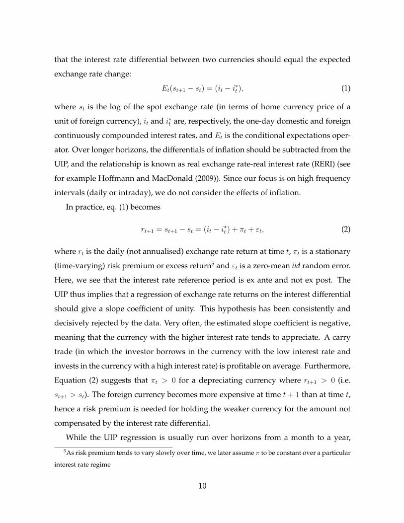
that the interest rate differential between two currencies should equal the expected

exchange rate change:

Et(st+1 − st) = (it − i∗t ), (1)

where st is the log of the spot exchange rate (in terms of home currency price of a

unit of foreign currency), it and i∗t are, respectively, the one-day domestic and foreign

continuously compounded interest rates, and Et is the conditional expectations oper-

ator. Over longer horizons, the differentials of inflation should be subtracted from the

UIP, and the relationship is known as real exchange rate-real interest rate (RERI) (see

for example Hoffmann and MacDonald (2009)). Since our focus is on high frequency

intervals (daily or intraday), we do not consider the effects of inflation.

In practice, eq. (1) becomes

rt+1 = st+1 − st = (it − i∗t ) + πt + εt, (2)

where rt is the daily (not annualised) exchange rate return at time t, πt is a stationary

(time-varying) risk premium or excess return5 and εt is a zero-mean iid random error.

Here, we see that the interest rate reference period is ex ante and not ex post. The

UIP thus implies that a regression of exchange rate returns on the interest differential

should give a slope coefficient of unity. This hypothesis has been consistently and

decisively rejected by the data. Very often, the estimated slope coefficient is negative,

meaning that the currency with the higher interest rate tends to appreciate. A carry

trade (in which the investor borrows in the currency with the low interest rate and

invests in the currency with a high interest rate) is profitable on average. Furthermore,

Equation (2) suggests that πt > 0 for a depreciating currency where rt+1 > 0 (i.e.

st+1 > st). The foreign currency becomes more expensive at time t + 1 than at time t,

hence a risk premium is needed for holding the weaker currency for the amount not

compensated by the interest rate differential.

While the UIP regression is usually run over horizons from a month to a year,

5As risk premium tends to vary slowly over time, we later assume π to be constant over a particular

interest rate regime

10

Lyons and Rose (1995) examine the relationship between interest differentials and

exchange rates at high frequency. They considered pairs of currencies in the now-

defunct European Monetary System (EMS), and found that currencies which were

under attack but in fact stayed within the band actually appreciated intraday. Lyons

and Rose argue that this intraday appreciation is a compensation for the risk of de-

valuation that might have occurred, but did not. Investors can be compensated for

the risk of devaluation only by intraday appreciation, not by interest differentials, as

there are effectively no interest rate differentials intraday at that time.

Similarly, Chaboud and Wright (2005) examine UIP over extremely short hori-

zons.6 An intraday UIP regression over a short period, that spans 17:00 New York

time when interest rate is paid, yielded results in favor of the UIP hypothesis. The

full overnight interest differential that accrues in such a window is offset by a jump

in the exchange rate. Positive results are obtained for relatively large discrete interest

payments accrue on positions held between Wednesday and Thursday, and especially

on the multi-day interest rate differential days in the weekend.

Based on current convention, investor received the interest rate differential dis-

cretely only at the point when a position was rolled over from one day to the next.

The common rollover time is determined by market convention. A position that was

not held open overnight received no interest rate differential because intra-daily inter-

est rates were often assumed to be zero. Today, transactions completed on blockchain

will attract interest rate for the duration that the asset is held, which is a fraction of

the daily rates (for example OIS-swap rates), which themselves may fluctuate intra-

day. However, our problem at hand is that the intraday rate for duration shorter than

a day (say 10 minutes) may not be a fraction of the overnight rate, but is dictated by

the supply and demand for the very short term borrowing/lending at the time.

6Chaboud and Wright (2005) use bilateral Japanese yen, German mark/euro, Swiss franc and pound

sterling 5-min average bid and ask spot exchange rates viz-a-viz the US dollar provided by Olsen and

Associates over the 15-year period 1988-2002 and discarding weekends, defined as the time from 23:00

GMT on Friday to 22:55 GMT on Sunday when there is virtually no foreign exchange trading.

11

3.2 Forecasting irregularly spaced intraday FX returns

To apply the UIP regression in Equation (2) requires a forecast for rt+1 at time t and

hence allows us to project the yield curve at time t for the ultra short tenor. To fully

exploit information contained in tick-by-tick quote or trade data, we adopt the time-

deformed model instead of the classical fixed time interval model. The origin of the

time-deformed model can be traced back to Clark (1973) who uses trading volume as

proxy for volatility, a finding which was later confirmed in Gallant et al. (1992). Later,

Ane and Geman (2000) extend Clark’s model by considering a general time change

process, and conclude that the transaction clock is better represented by number of

trades than volume of trades. The larger the number of trades, the smaller the du-

ration between trades. More recently, Feng et al. (2015) estimated a time-deformed

model for IBM stock returns with latent stochastic volatility using the method of sim-

ulated moments.7

In a similar approach, Engle and Russell (1998) and Engle (2000) model directly

transaction arrival times as stochastic events in the form of joint marked point pro-

cesses. The FX quotes or transaction returns can be modeled as two simultaneous

random processes- durations dk and returns rk, where the joint density can be ex-

pressed as the product of the marginal density of duration and the conditional density

of returns given duration:

f(dk, rk|dk−1, rk−1; θk) = g(dk|dk−1, rk−1; θ1k)q(rk|dk, dk−1, rk−1; θ2k) (3)

where xk = {xk, xk−1, . . . , x1} denotes the past of x and θs are parameters of the con-

ditional densities. To model the durations process, we use the log-ACD model of

Bauwens and Giot (2000), which is the logarithmic version of the ACD model of En-

gle and Russell (1998). The duration between two quotes or transactions is expressed

7Feng et al. (2015)’s choice of MSM (Method of Simulated Moments) is motivated by the analytically

intractable likelihood function. We decided against this model after having difficulty with optimizing

globally over all parameters when the sample includes an extremely large amount of data. The esti-

mated model is very sensitive to the starting values used.

12

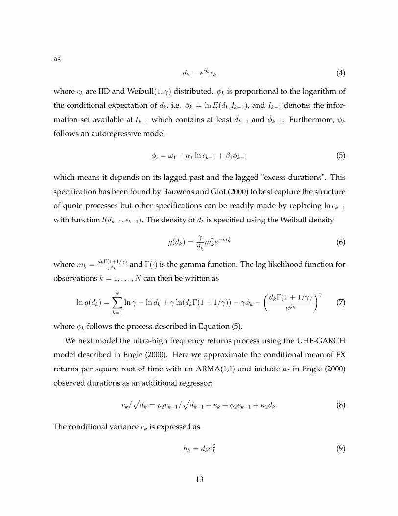
as

dk = eφkεk (4)

where εk are IID and Weibull(1, γ) distributed. φk is proportional to the logarithm of

the conditional expectation of dk, i.e. φk = lnE(dk|Ik−1), and Ik−1 denotes the infor-

mation set available at tk−1 which contains at least dk−1 and φk−1. Furthermore, φk

follows an autoregressive model

φi = ω1 + α1 ln εk−1 + β1φk−1 (5)

which means it depends on its lagged past and the lagged "excess durations". This

specification has been found by Bauwens and Giot (2000) to best capture the structure

of quote processes but other specifications can be readily made by replacing ln εk−1

with function l(dk−1, εk−1). The density of dk is specified using the Weibull density

g(dk) =γ

dkmγke−mγk (6)

where mk = dkΓ(1+1/γ)

eφkand Γ(·) is the gamma function. The log likelihood function for

observations k = 1, . . . , N can then be written as

ln g(dk) =N∑k=1

ln γ − ln dk + γ ln(dkΓ(1 + 1/γ))− γφk −(dkΓ(1 + 1/γ)

eφk

)γ(7)

where φk follows the process described in Equation (5).

We next model the ultra-high frequency returns process using the UHF-GARCH

model described in Engle (2000). Here we approximate the conditional mean of FX

returns per square root of time with an ARMA(1,1) and include as in Engle (2000)

observed durations as an additional regressor:

rk/√dk = ρ2rk−1/

√dk−1 + ek + φ2ek−1 + κ2dk. (8)

The conditional variance rk is expressed as

hk = dkσ2k (9)

13

where σ2k is the conditional volatility per unit of time which can be modelled as a

GARCHX(1,1) process

σ2k = ω2 + α2e

2k−1 + β2σ

2k−1 + γ2d

−1k (10)

in which the conditional variance depends on the reciprocal of duration. The the-

ory concerning duration and volatility is well debated in the literature. According to

market microstructure theory (see Easley and O’Hara (1992)), clusters of return inno-

vations are observed in the market when an unexpected piece of information arrives

producing very frequent transactions with very short durations. In contrast, large du-

ration should have lower volatility and lower adverse selection cost. On the empirical

front, Manganelli (2005) finds that, for heavily traded stocks, volatility has a signifi-

cant and negative impact on duration; low durations follow large volatilities. How-

ever, in an order-driven (instead of pricing-driven) market, when volatility is large,

traders will be encouraged to provide liquidity and hence discouraged to trade im-

mediately. This is because trading during a high volatility episode would incur both

higher cost of the liquidity consumption and higher benefit of the liquidity provision.

This means that a higher volatility should lead to a higher duration. In Equation (10),

exchange rate volatility is a function of duration, dk, whose direction of the impact

will be determined by the sign of γ2.

In the event of a flash crash, we can add an indicator variable Ik to Equation (8) or

(10) that takes a value of 1 for a structural break after a flash event and zero otherwise.

This controls for the effect of the flash event and we assume here that the flash crash

is temporary and its onset is known a priori.

Since the UHF-GARCH model can also be estimated using maximum likelihood,

the overall time-deformed log ACD UHF-GARCH process can be estimated jointly

using the log likelihood:

LL =N∑k=1

[ln g(dk|dk−1, rk−1; θ1) + ln q(rk|dk, dk−1, rk−1; θ2)], (11)

where θ1 = {ω1, α1, β1, γ} and θ2 = {ρ2, φ2, ω2, α2, β2, γ2}

14

3.3 Constructing the ultra short tenor yield curve

To construct the ultra short tenor yield curve8, we estimate the log-ACD UHF-

GARCH model at time tk using the last 1000 quote observations and use the esti-

mated parameters to simulate the next 5000 time-deformed observations. We repeat

the simulations 1000 times, i.e. we construct 1000 projected yield curves and take the

average.9

Using UIP, the ultra short tenor yield curve an investor faces at time t = tk to hold

an asset till time t = tk + tq is

q∑j=1

rk+j = (ik+q − i∗k+q) +

(q∑j=1

δk+j

)π + εk, q = 1, . . . , N (12)

where δk = dkD

is the duration dk expressed as a fraction of a business day, D, both

measured in the same time units (assuming that a business day is 24 hours), and N

is the number of irregularly spaced quotes/observations. π is the daily exchange rate

risk premium for a particular day, which arguably is a function of the volatility and

can potentially be negative or zero as well depending on the relative strength of the

two currencies. We assume π to be constant over a particular interest rate regime and

estimate it using Equation (2) with daily data over the past one year. We also assume

that it is ’constant’ intraday, scaled by intraday duration that the asset is held.

The intraday interest rates, ik+q and i∗k+q, are the unscaled (i.e. not converted to

daily or annual) local and foreign interest rates in basis points charged or paid over

the∑q

j=1 dk+j duration at time tk. If intraday interest rates are constant for day t, then

the net interest differential is simply (ik+q − i∗k+q) =∑q

j=1 δk+j(it − i∗t ), where it and i∗t

8The "yield curve" here denotes market risk-free interest rates, in contrast to Treasury curves, which

are relevant only for sovereign, or Libor, and are not free from credit risks.9The choice of using 1000 in-sample observations for estimations is arbitrary and constitutes for

our dataset of the last 2-3 hours observations. Shortly after the crash on 15 Jan at 10a.m., the last

1000 observations consists of the last 1.5 hours of observations. One could also use for example all

observations in the last hour, etc. Further fine-tuning for optimal in- and out-of-sample sizes could be

made but is out-of-scope of this paper.

15

are the local and foreign daily overnight rates respectively for day t. In the case where

i∗k+q is known, Equation (12) can be used to infer ik+q, and vice versa.

Given q = 1, . . . , N estimated values of ik+q and dk+q, we fit the Nelson-Siegel

model to the time-deformed model-simulated yield curve to produce the fitted intra-

day yield curve10 as follows:

ik+q = b0 + b1[1− exp(−d/τ)]

d/τ+ b2

([1− exp(−d/τ)]

d/τ− exp(−d/τ)

)(13)

where b0, b1, b2 and τ are the fitted parameters.11

According to Nelson and Siegel (1987), b0 is interpreted as the long run levels of

interest rates (the loading is 1, it is a constant that does not decay), b1 is the short-

term component (it starts at 1, and decays monotonically and quickly to 0), b2 is the

medium-term component (it starts at 0, increases, then decays to zero), and τ is the

decay factor: small values produce slow decay and can better fit the curve at long

maturities, while large values produce fast decay and can better fit the curve at short

maturities, τ also governs where b2 achieves its maximum. In order to constrain ik+q to

the overnight rate it when∑q

j=1 dk+j equals one day, we do not estimate b0 but simply

10We use the unscaled intraday yield curve. We can express the rates as daily rates by using ik+q

the scaled (daily) rate for intraday duration∑q

j=1 dk+j (i.e. ik+q = ik+q/∑q

j=1 δk+j). We find however,

due to the large effect of scaling where there are 86400 seconds in a day, it renders most of the yield

curve very flat except for the first six minutes. For ease of reading of the graph, we use the unscaled

interest rates.11In the case when i∗k+q is also unknown, we propose using cross rate parity of two FX returns to help

estimate ik+q . For example, to estimate the intraday yield curve for CHF, both forecasted EURCHF and

USDCHF FX returns can be used to estimate ik+q,CHF :

q∑j=1

rk+j,EURCHF −q∑

j=1

δk+jπEURCHF = (ik+q,EUR − ik+q,CHF ) + εk,EURCHF , q = 1, . . . , N (14)

q∑j=1

rk+j,USDCHF −q∑

j=1

δk+jπUSDCHF = (ik+q,USD − ik+q,CHF ) + εk,USDCHF , q = 1, . . . , N (15)

where ik+q,EUR and ik+q,USD are estimated using daily rates scaled by the intraday durations, i∗k+q =

it/∑q

j=1 dk+j . Expectation Maximization (EM) algorithm can be used to fit the Nelson Siegel curve

using both the estimated ik+q,CHF in (14) and (15).

16

use b0 = it, the 1-day unscaled rate, i.e. the intraday yield curve should converge to

the daily ’long run’ yield, except during flash crashes when the ON rates may be stale.

4 An Empirical Study: Swiss Franc Event, 15 January

2015

On 15 January 2015, SNB announced at 09:30 (local time) the discontinuation of

the minimum exchange rate of CHF 1.20 per euro. At the same time, it lowered the

interest rate on sight deposit account balances by 0.5 percentage points, to -0.75%, and

the target range for the three-month Libor was to change from between -0.75% and

0.25% to between -1.25% and -0.25%. Prior to the SNB’s intervention, the euro has

depreciated considerably against the US dollar and this, in turn, has caused the Swiss

franc to weaken against the US dollar. Hence, the SNB concluded that enforcing and

maintaining the minimum exchange rate for the Swiss franc against the euro is no

longer justified.

The SNB announcement caused a 41% rise in the Swiss franc in 20 minutes. It

retracted over 60% of this move within a further 20 minutes. Automated liquidity

providers withdrew from two-sided market-making and suspended streaming prices

on public and bilateral platforms. Chicago Mercantile Exchange activated a trading

halt in CHF currency futures which further amplified the flash crash. Later, the SNB

stabilised markets by providing liquidity in a price range, giving market participants

the confidence to re-enter the market. Market users initially reverted to more tradi-

tional transaction methods such as voice trading but resumed the use of all method-

ologies once they had made the appropriate adjustments to their e-trading tools.

4.1 Data

We use intraday EURCHF and USDCHF quote data from Olsen for the period 08

-16 January 2015. The data contains tick-by-tick quotes with time stamps in millisec-

17

onds, bid and ask prices and bid and ask volumes. FX trading is 24 hours, hence

we include the overnight period but exclude all weekend quotes (because of too few

observations) which leaves us with seven days of data. For quotes within the same

second, we keep only the last entry of the second (with the largest millisecond) as a

representative observation.12 To compute FX returns, we use the log returns of the

midprice, i.e.

Rk = ln(Askk +Bidk

2)− ln(

Askk−1 +Bidk−1

2)

Tables 1 shows the number of observations for EURCHF and USDCHF respec-

tively, each day before and after ’filtering’ the data (from multiple quotes within a

second) as well as the descriptive statistics of the quote returns and durations. Market

liquidity of USDCHF is higher than that of EURCHF, with significantly more quotes

and much shorter quote durations. With exception of 15 January, the returns of USD-

CHF are also more volatile than EURCHF.

[Table 1 about here.]

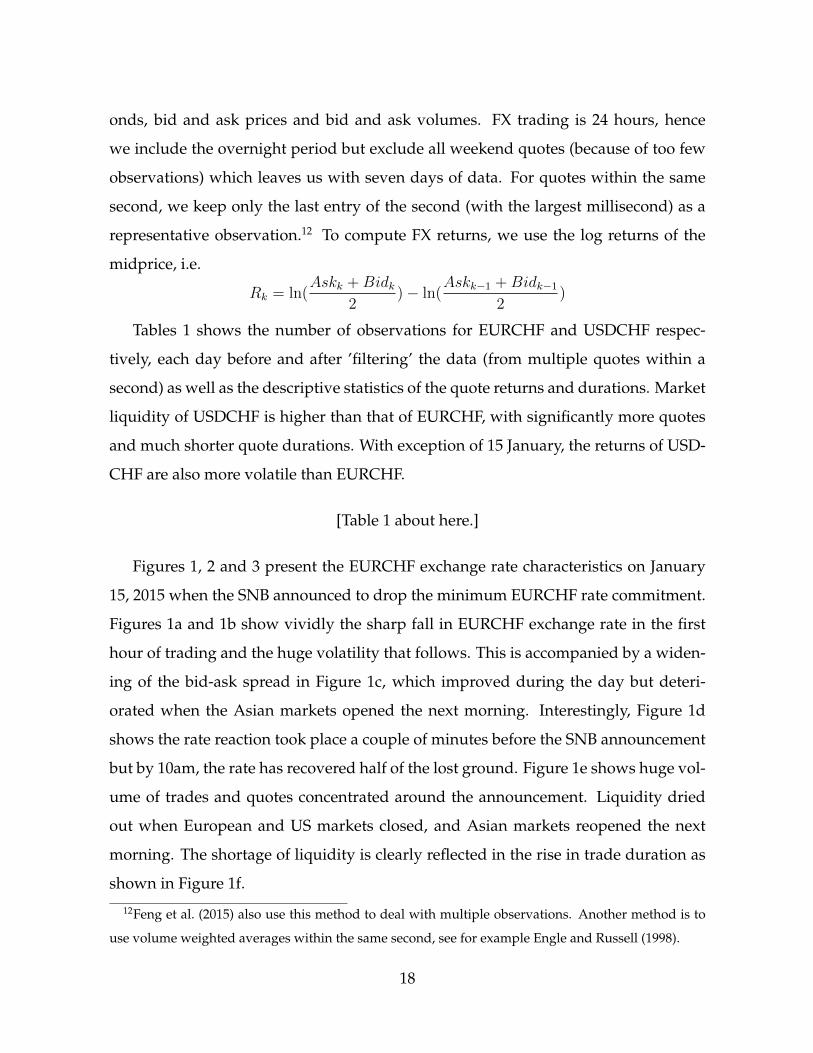
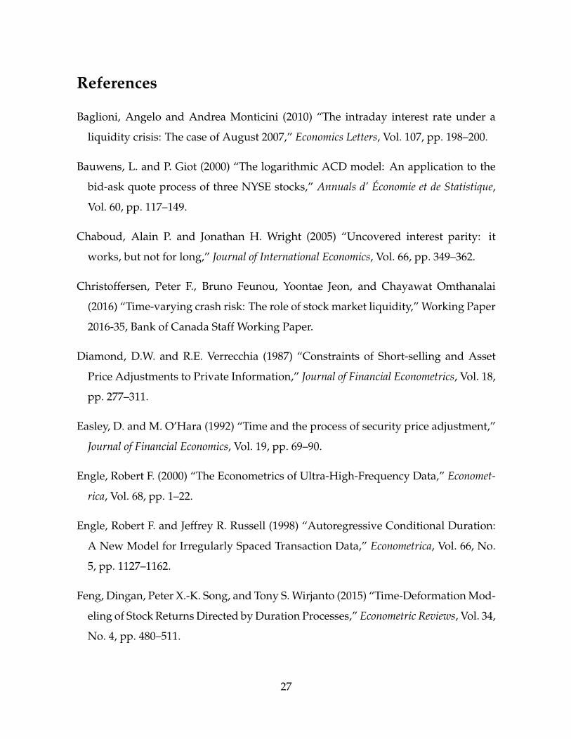
Figures 1, 2 and 3 present the EURCHF exchange rate characteristics on January

15, 2015 when the SNB announced to drop the minimum EURCHF rate commitment.

Figures 1a and 1b show vividly the sharp fall in EURCHF exchange rate in the first

hour of trading and the huge volatility that follows. This is accompanied by a widen-

ing of the bid-ask spread in Figure 1c, which improved during the day but deteri-

orated when the Asian markets opened the next morning. Interestingly, Figure 1d

shows the rate reaction took place a couple of minutes before the SNB announcement

but by 10am, the rate has recovered half of the lost ground. Figure 1e shows huge vol-

ume of trades and quotes concentrated around the announcement. Liquidity dried

out when European and US markets closed, and Asian markets reopened the next

morning. The shortage of liquidity is clearly reflected in the rise in trade duration as

shown in Figure 1f.

12Feng et al. (2015) also use this method to deal with multiple observations. Another method is to

use volume weighted averages within the same second, see for example Engle and Russell (1998).

18

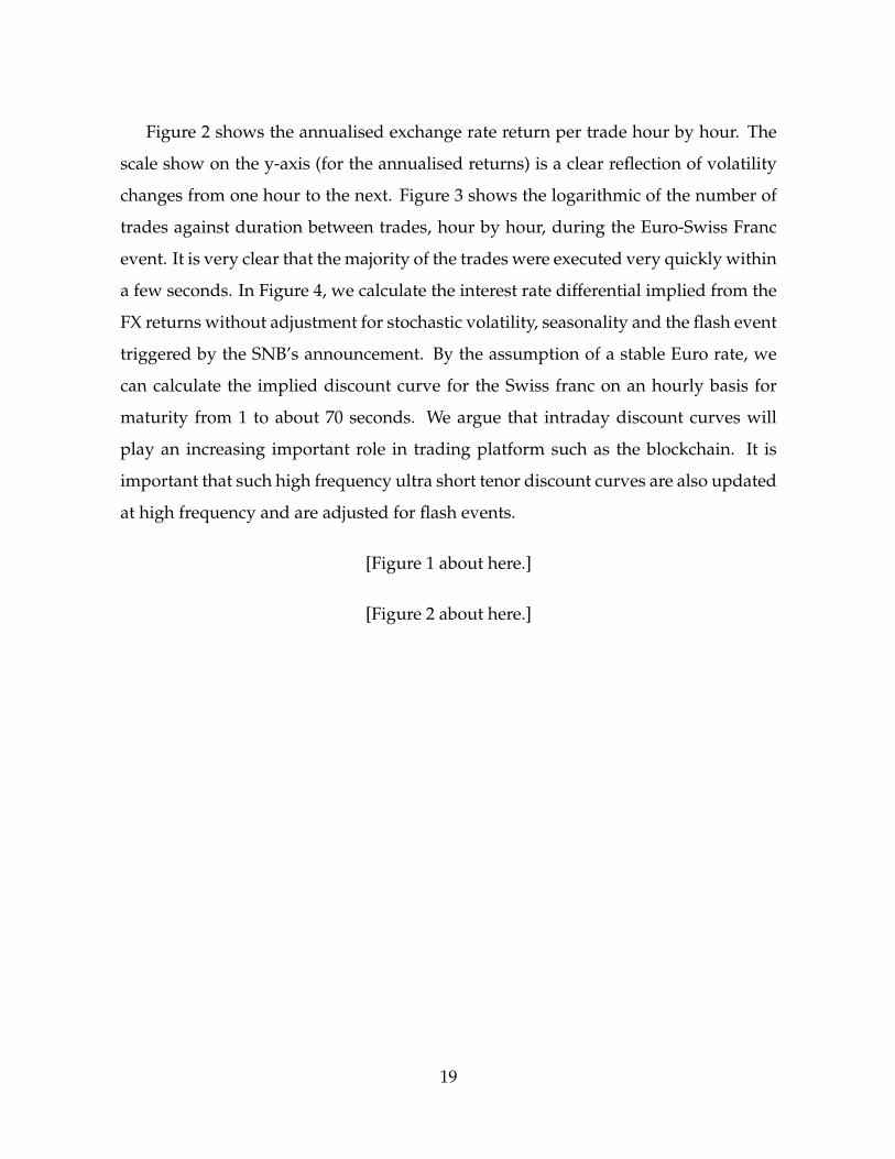
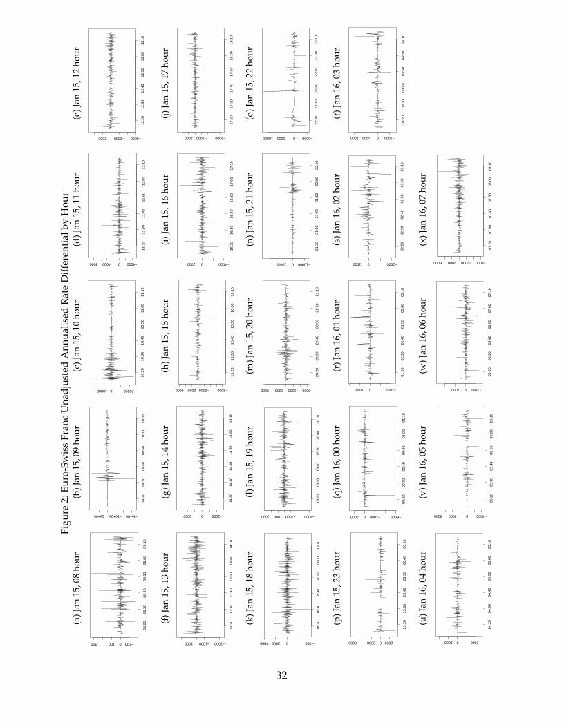
Figure 2 shows the annualised exchange rate return per trade hour by hour. The

scale show on the y-axis (for the annualised returns) is a clear reflection of volatility

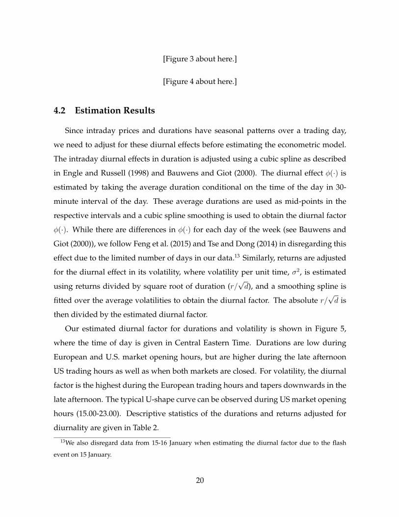
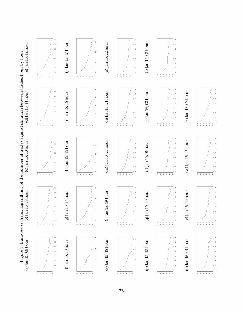
changes from one hour to the next. Figure 3 shows the logarithmic of the number of

trades against duration between trades, hour by hour, during the Euro-Swiss Franc

event. It is very clear that the majority of the trades were executed very quickly within

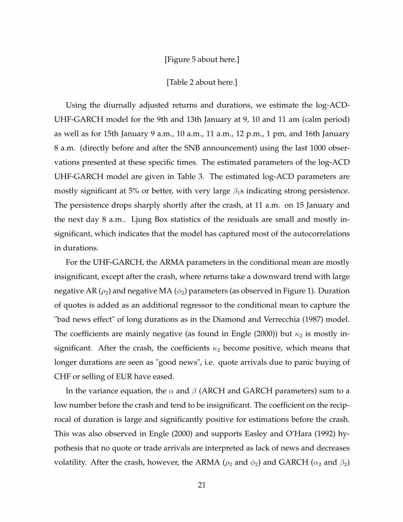
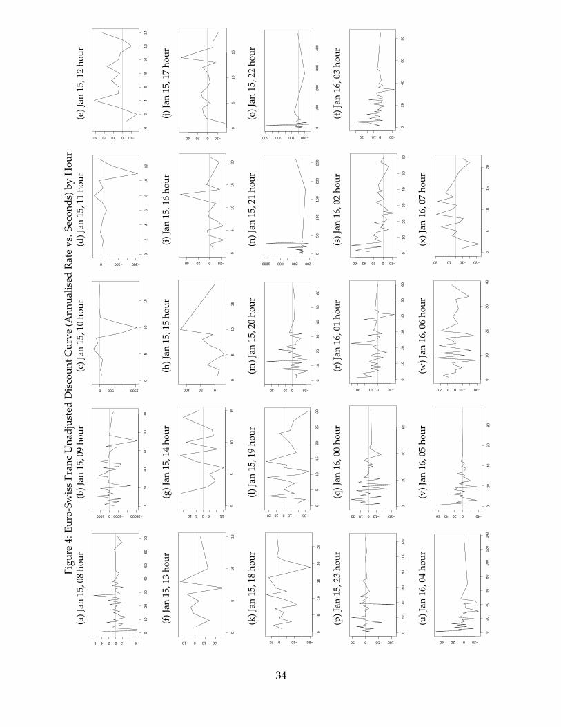
a few seconds. In Figure 4, we calculate the interest rate differential implied from the

FX returns without adjustment for stochastic volatility, seasonality and the flash event

triggered by the SNB’s announcement. By the assumption of a stable Euro rate, we

can calculate the implied discount curve for the Swiss franc on an hourly basis for

maturity from 1 to about 70 seconds. We argue that intraday discount curves will

play an increasing important role in trading platform such as the blockchain. It is

important that such high frequency ultra short tenor discount curves are also updated

at high frequency and are adjusted for flash events.

[Figure 1 about here.]

[Figure 2 about here.]

19

[Figure 3 about here.]

[Figure 4 about here.]

4.2 Estimation Results

Since intraday prices and durations have seasonal patterns over a trading day,

we need to adjust for these diurnal effects before estimating the econometric model.

The intraday diurnal effects in duration is adjusted using a cubic spline as described

in Engle and Russell (1998) and Bauwens and Giot (2000). The diurnal effect φ(·) is

estimated by taking the average duration conditional on the time of the day in 30-

minute interval of the day. These average durations are used as mid-points in the

respective intervals and a cubic spline smoothing is used to obtain the diurnal factor

φ(·). While there are differences in φ(·) for each day of the week (see Bauwens and

Giot (2000)), we follow Feng et al. (2015) and Tse and Dong (2014) in disregarding this

effect due to the limited number of days in our data.13 Similarly, returns are adjusted

for the diurnal effect in its volatility, where volatility per unit time, σ2, is estimated

using returns divided by square root of duration (r/√d), and a smoothing spline is

fitted over the average volatilities to obtain the diurnal factor. The absolute r/√d is

then divided by the estimated diurnal factor.

Our estimated diurnal factor for durations and volatility is shown in Figure 5,

where the time of day is given in Central Eastern Time. Durations are low during

European and U.S. market opening hours, but are higher during the late afternoon

US trading hours as well as when both markets are closed. For volatility, the diurnal

factor is the highest during the European trading hours and tapers downwards in the

late afternoon. The typical U-shape curve can be observed during US market opening

hours (15.00-23.00). Descriptive statistics of the durations and returns adjusted for

diurnality are given in Table 2.

13We also disregard data from 15-16 January when estimating the diurnal factor due to the flash

event on 15 January.

20

[Figure 5 about here.]

[Table 2 about here.]

Using the diurnally adjusted returns and durations, we estimate the log-ACD-

UHF-GARCH model for the 9th and 13th January at 9, 10 and 11 am (calm period)

as well as for 15th January 9 a.m., 10 a.m., 11 a.m., 12 p.m., 1 pm, and 16th January

8 a.m. (directly before and after the SNB announcement) using the last 1000 obser-

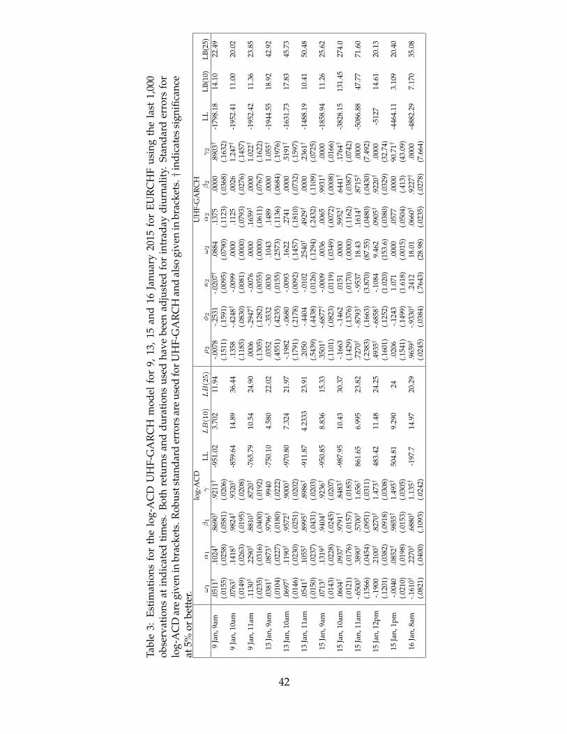
vations presented at these specific times. The estimated parameters of the log-ACD

UHF-GARCH model are given in Table 3. The estimated log-ACD parameters are

mostly significant at 5% or better, with very large β1s indicating strong persistence.

The persistence drops sharply shortly after the crash, at 11 a.m. on 15 January and

the next day 8 a.m.. Ljung Box statistics of the residuals are small and mostly in-

significant, which indicates that the model has captured most of the autocorrelations

in durations.

For the UHF-GARCH, the ARMA parameters in the conditional mean are mostly

insignificant, except after the crash, where returns take a downward trend with large

negative AR (ρ2) and negative MA (φ2) parameters (as observed in Figure 1). Duration

of quotes is added as an additional regressor to the conditional mean to capture the

"bad news effect" of long durations as in the Diamond and Verrecchia (1987) model.

The coefficients are mainly negative (as found in Engle (2000)) but κ2 is mostly in-

significant. After the crash, the coefficients κ2 become positive, which means that

longer durations are seen as "good news", i.e. quote arrivals due to panic buying of

CHF or selling of EUR have eased.

In the variance equation, the α and β (ARCH and GARCH parameters) sum to a

low number before the crash and tend to be insignificant. The coefficient on the recip-

rocal of duration is large and significantly positive for estimations before the crash.

This was also observed in Engle (2000) and supports Easley and O’Hara (1992) hy-

pothesis that no quote or trade arrivals are interpreted as lack of news and decreases

volatility. After the crash, however, the ARMA (ρ2 and φ2) and GARCH (α2 and β2)

21

parameters become very large (summing to more than one) and significant, while

the coefficients on inverse durations (γ2) becomes insignificant. This high estimated

persistence is an artefact of the extreme observations in the sample period. The low

Ljung-Box statistics in the residuals indicates that the UHF-GARCH model has cap-

tured much of the autocorrelation in intraday return.

[Table 3 about here.]

Using only the estimated parameters that are significant, we simulate a horizon of

5000 time-deformed observations starting with the last observation in the sample. The

simulations are repeated 1000 times and then the mean durations (dk) and returns (rk)

are used. The diurnal factors are re-introduced into the mean simulated durations

and returns. We then use the simulated data to estimate the UIP equation (12). To

estimate the exchange rate risk premium (in Equation (2)), we use the daily EURCHF14

and interest rates of the last one year preceeding our dataset and obtain a daily risk

premium estimate for the period of π = 1.746× 10−4.

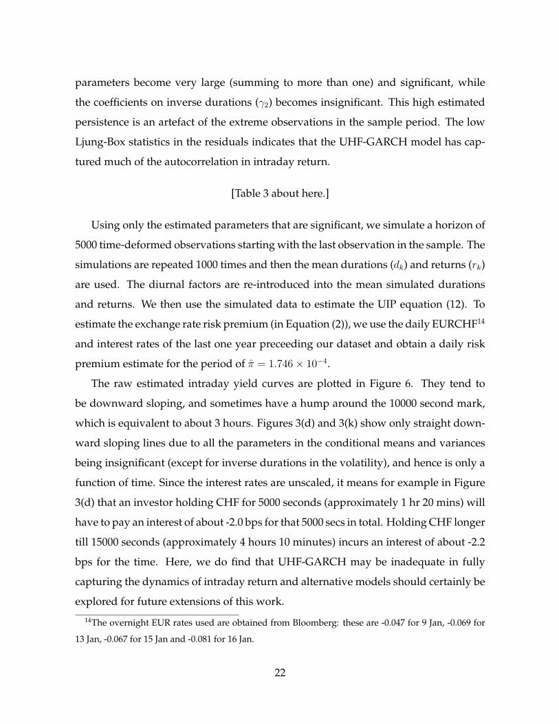
The raw estimated intraday yield curves are plotted in Figure 6. They tend to

be downward sloping, and sometimes have a hump around the 10000 second mark,

which is equivalent to about 3 hours. Figures 3(d) and 3(k) show only straight down-

ward sloping lines due to all the parameters in the conditional means and variances

being insignificant (except for inverse durations in the volatility), and hence is only a

function of time. Since the interest rates are unscaled, it means for example in Figure

3(d) that an investor holding CHF for 5000 seconds (approximately 1 hr 20 mins) will

have to pay an interest of about -2.0 bps for that 5000 secs in total. Holding CHF longer

till 15000 seconds (approximately 4 hours 10 minutes) incurs an interest of about -2.2

bps for the time. Here, we do find that UHF-GARCH may be inadequate in fully

capturing the dynamics of intraday return and alternative models should certainly be

explored for future extensions of this work.

14The overnight EUR rates used are obtained from Bloomberg: these are -0.047 for 9 Jan, -0.069 for

13 Jan, -0.067 for 15 Jan and -0.081 for 16 Jan.

22

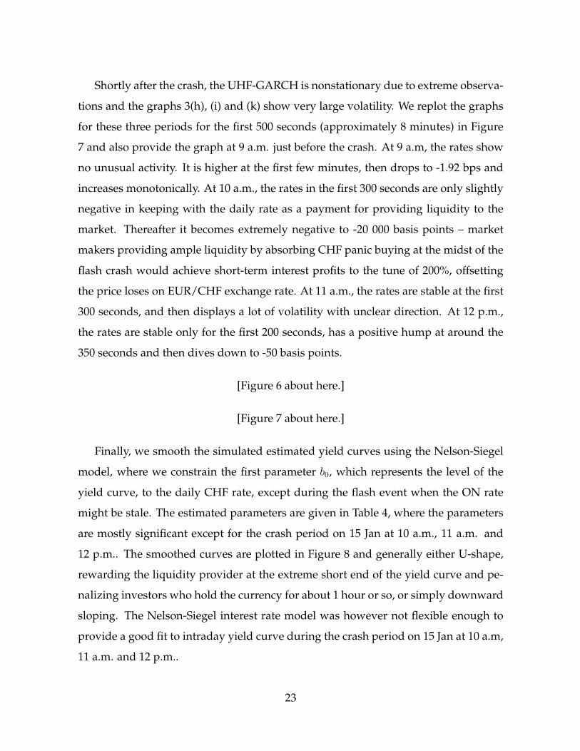
Shortly after the crash, the UHF-GARCH is nonstationary due to extreme observa-

tions and the graphs 3(h), (i) and (k) show very large volatility. We replot the graphs

for these three periods for the first 500 seconds (approximately 8 minutes) in Figure

7 and also provide the graph at 9 a.m. just before the crash. At 9 a.m, the rates show

no unusual activity. It is higher at the first few minutes, then drops to -1.92 bps and

increases monotonically. At 10 a.m., the rates in the first 300 seconds are only slightly

negative in keeping with the daily rate as a payment for providing liquidity to the

market. Thereafter it becomes extremely negative to -20 000 basis points – market

makers providing ample liquidity by absorbing CHF panic buying at the midst of the

flash crash would achieve short-term interest profits to the tune of 200%, offsetting

the price loses on EUR/CHF exchange rate. At 11 a.m., the rates are stable at the first

300 seconds, and then displays a lot of volatility with unclear direction. At 12 p.m.,

the rates are stable only for the first 200 seconds, has a positive hump at around the

350 seconds and then dives down to -50 basis points.

[Figure 6 about here.]

[Figure 7 about here.]

Finally, we smooth the simulated estimated yield curves using the Nelson-Siegel

model, where we constrain the first parameter b0, which represents the level of the

yield curve, to the daily CHF rate, except during the flash event when the ON rate

might be stale. The estimated parameters are given in Table 4, where the parameters

are mostly significant except for the crash period on 15 Jan at 10 a.m., 11 a.m. and

12 p.m.. The smoothed curves are plotted in Figure 8 and generally either U-shape,

rewarding the liquidity provider at the extreme short end of the yield curve and pe-

nalizing investors who hold the currency for about 1 hour or so, or simply downward

sloping. The Nelson-Siegel interest rate model was however not flexible enough to

provide a good fit to intraday yield curve during the crash period on 15 Jan at 10 a.m,

11 a.m. and 12 p.m..

23

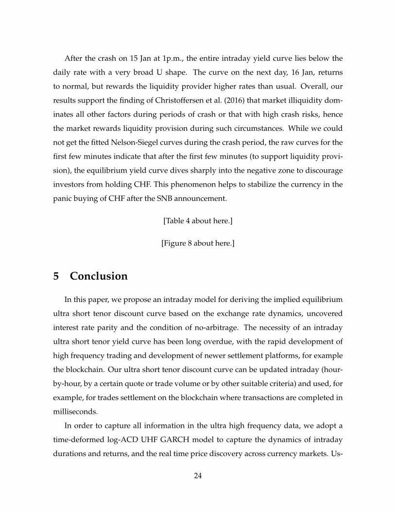
After the crash on 15 Jan at 1p.m., the entire intraday yield curve lies below the

daily rate with a very broad U shape. The curve on the next day, 16 Jan, returns

to normal, but rewards the liquidity provider higher rates than usual. Overall, our

results support the finding of Christoffersen et al. (2016) that market illiquidity dom-

inates all other factors during periods of crash or that with high crash risks, hence

the market rewards liquidity provision during such circumstances. While we could

not get the fitted Nelson-Siegel curves during the crash period, the raw curves for the

first few minutes indicate that after the first few minutes (to support liquidity provi-

sion), the equilibrium yield curve dives sharply into the negative zone to discourage

investors from holding CHF. This phenomenon helps to stabilize the currency in the

panic buying of CHF after the SNB announcement.

[Table 4 about here.]

[Figure 8 about here.]

5 Conclusion

In this paper, we propose an intraday model for deriving the implied equilibrium

ultra short tenor discount curve based on the exchange rate dynamics, uncovered

interest rate parity and the condition of no-arbitrage. The necessity of an intraday

ultra short tenor yield curve has been long overdue, with the rapid development of

high frequency trading and development of newer settlement platforms, for example

the blockchain. Our ultra short tenor discount curve can be updated intraday (hour-

by-hour, by a certain quote or trade volume or by other suitable criteria) and used, for

example, for trades settlement on the blockchain where transactions are completed in

milliseconds.

In order to capture all information in the ultra high frequency data, we adopt a

time-deformed log-ACD UHF GARCH model to capture the dynamics of intraday

durations and returns, and the real time price discovery across currency markets. Us-

24

ing the estimated model, we simulate time-deformed observations for a full range

of ultra short tenor interest rates and construct a yield curve based on UIP. We then

estimate a smoothed Nelson-Siegel yield curve using nonlinear least squares. We

find that the log-ACD models intraday durations effectively but the fit of the UHF-

GARCH model for tick-by-tick quote returns are at times poor using our FX dataset.

We also find that the Nelson-Siegel curve is not flexible enough to obtain smoothed ul-

tra short tenor discount curves during flash crashes, and future work should consider

developing other models for such purpose.

Our findings show that the intraday yield curve update is generally U-shape or

downward sloping, where liquidity provision is rewarded with higher interest rates

in the first few minutes, and holding the currency for an hour or more incurs costs

to the investor. During the crash triggered by the SNB announcement, the first five

minutes of the intraday yield curve is still stable, but after that dives sharply to -

20000 basis points in the first hour after the announcement. This very negative rates

incentivizes liquidity provision, discourages investors from the panic buying of CHF

and should automatically stabilize the currency in the short term before the effect of

the daily interest rate adjustment kicks in at the end of the day. The next day after the

crash, we notice large interest rates at the very short end of the intraday yield curve

to encourage liquidity provision. This supports the hypothesis of Christoffersen et al.

(2016) of market liquidity factor dominating during periods with high crash risks.

This paper is a first novel attempt at introducing an intraday ultra short tenor yield

curve following the FXWG’s code. We derive the intraday yield curves that is consis-

tent with market liquidity provision and discourage ultra short term speculation that

increases crash risks. During periods of shocks, the stabilizing mechanism of intra-

day interest rates become even more critical and lend central banks a useful tool in

managing the stability of their currencies. The flash crash on January 15 saw the EU-

RCHF fall by 40% in seconds. While FX trading venues could trigger circuit breakers

to prevent extreme pricing, the execution system could not function properly because

liquidity providers ceased to provide liquidity during the event. We strongly argue

25

that had such ultra short tenor interest rates adjustments been implemented, many

large swings in currency trades would have been prevented.

26

References

Baglioni, Angelo and Andrea Monticini (2010) “The intraday interest rate under a

liquidity crisis: The case of August 2007,” Economics Letters, Vol. 107, pp. 198–200.

Bauwens, L. and P. Giot (2000) “The logarithmic ACD model: An application to the

bid-ask quote process of three NYSE stocks,” Annuals d’ Économie et de Statistique,

Vol. 60, pp. 117–149.

Chaboud, Alain P. and Jonathan H. Wright (2005) “Uncovered interest parity: it

works, but not for long,” Journal of International Economics, Vol. 66, pp. 349–362.

Christoffersen, Peter F., Bruno Feunou, Yoontae Jeon, and Chayawat Omthanalai

(2016) “Time-varying crash risk: The role of stock market liquidity,” Working Paper

2016-35, Bank of Canada Staff Working Paper.

Diamond, D.W. and R.E. Verrecchia (1987) “Constraints of Short-selling and Asset

Price Adjustments to Private Information,” Journal of Financial Econometrics, Vol. 18,

pp. 277–311.

Easley, D. and M. O’Hara (1992) “Time and the process of security price adjustment,”

Journal of Financial Economics, Vol. 19, pp. 69–90.

Engle, Robert F. (2000) “The Econometrics of Ultra-High-Frequency Data,” Economet-

rica, Vol. 68, pp. 1–22.

Engle, Robert F. and Jeffrey R. Russell (1998) “Autoregressive Conditional Duration:

A New Model for Irregularly Spaced Transaction Data,” Econometrica, Vol. 66, No.

5, pp. 1127–1162.

Feng, Dingan, Peter X.-K. Song, and Tony S. Wirjanto (2015) “Time-Deformation Mod-

eling of Stock Returns Directed by Duration Processes,” Econometric Reviews, Vol. 34,

No. 4, pp. 480–511.

27

Golub, A., A. Dupuis, and R. Olsen (2013) “High Frequency Trading Strategies in

FX Markets,” in David Easley, Marcos López de Prado, and Maureen O’Hara eds.

High-Frequency Trading- New Realities for Traders, Markets and Regulators: Risk Books.

Hansen, L.P. and R.J. Hodrick (1980) “Forward exchange rates as optimal predictors

of future spot rates: an econometric analysis.,” Journal of Political Economy, Vol. 88,

pp. 829–853.

Hoffmann, Mathias and Ronald MacDonald (2009) “Real exchange rates and real in-

terest rate differentials: A present value interpretation,” European Economic Review,

Vol. 53, pp. 952–970.

Kirilenko, Andrei, Albert S. Kyle, Mehrdad Samadi, and Tugkan Tuzun (2014) “The

Flash Crash: High Frequency Trading in an Electronic Market,” working paper, U.S.

Commodity Futures Trading Commission.

Lyons, R.K. and A.K. Rose (1995) “Explaining forward exchange intraday bias,” Jour-

nal of Finance, Vol. 50, pp. 1321–1329.

Manganelli (2005) “Duration, Volume, and the Price impact of trades,” Journal of Fi-

nancial Markets, Vol. 8, pp. 377–399.

McKinsey (2015) “Beyond the Hype: Blockchains in Capital Markets,” Working Pa-

pers on Corporate & Investment Banking 12, McKinsey&Company.

Özatay, Fatih (2002) “Turkey’s 2000-2001 Financial Crisis and the Central Bank’s Pol-

icy in the Aftermath of the Crisis,” working paper, Bank of Albania ’In the second

decade of transition’ Conference.

Peters, Gareth W. and Efstathios Panayi (2016) “Understanding Modern Banking

Ledgers through Blockchain Technologies: Future of Transaction Processing and

Smart Contracts on the Internet of Money,” in P Tasca, T. Aste, L. Pelizzon, and

N. Perony eds. Banking Beyond Banks and Money: Springer.

28

Tse, Yiu-Kuen and Yingjie Dong (2014) “Intraday periodicity adjustments of transac-

tion duration and their effects on high-frequency volatility estimation,” Journal of

Empirical Finance, Vol. 28, pp. 352–361.

29

List of Figures

1 Euro-Swiss Franc Exchange Rate . . . . . . . . . . . . . . . . . . . . . . 312 Euro-Swiss Franc Unadjusted Annualised Rate Differential by Hour . 323 Euro-Swiss Franc: logarithmic of the number of trades against duration

between trades, hour by hour . . . . . . . . . . . . . . . . . . . . . . . . 334 Euro-Swiss Franc Unadjusted Discount Curve (Annualised Rate vs. Sec-

onds) by Hour . . . . . . . . . . . . . . . . . . . . . . . . . . . . . . . . . 345 Diurnal effects in durations and volatility: Black broken lines show the

average time-of-day effect of durations. Red lines show the smootheddiurnal factor using cubic splines. Time of day is given in Central East-ern Time. . . . . . . . . . . . . . . . . . . . . . . . . . . . . . . . . . . . . 35

6 CHF Unadjusted Yield Curves . . . . . . . . . . . . . . . . . . . . . . . 367 CHF Unadjusted Yield Curves just before and after SNB announcement

at the ultra short end tenor. . . . . . . . . . . . . . . . . . . . . . . . . . 378 Estimated CHF Nielsen Siegel Yield Curves . . . . . . . . . . . . . . . . 38

30

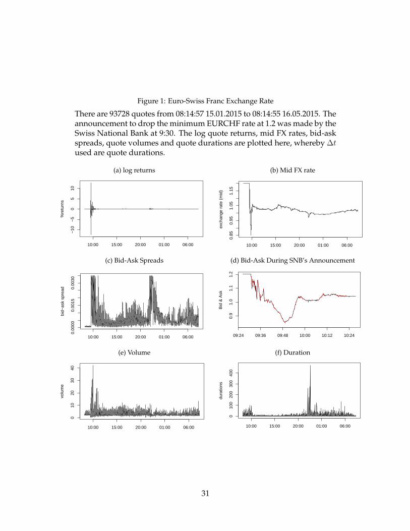
Figure 1: Euro-Swiss Franc Exchange Rate

There are 93728 quotes from 08:14:57 15.01.2015 to 08:14:55 16.05.2015. Theannouncement to drop the minimum EURCHF rate at 1.2 was made by theSwiss National Bank at 9:30. The log quote returns, mid FX rates, bid-askspreads, quote volumes and quote durations are plotted here, whereby ∆tused are quote durations.

(a) log returns

10:00 15:00 20:00 01:00 06:00

−10

−5

05

10

time

%re

turn

s

(b) Mid FX rate

10:00 15:00 20:00 01:00 06:00

0.85

0.95

1.05

1.15

time

exch

ange

rat

e (m

id)

(c) Bid-Ask Spreads

10:00 15:00 20:00 01:00 06:00

0.00

000.

0015

0.00

30

time

bid−

ask

spre

ad

(d) Bid-Ask During SNB’s Announcement

09:24 09:36 09:48 10:00 10:12 10:24

0.9

1.0

1.1

1.2

Bid

& A

sk

(e) Volume

10:00 15:00 20:00 01:00 06:00

010

2030

40

time

volu

me

(f) Duration

10:00 15:00 20:00 01:00 06:00

010

020

030

040

0

time

dura

tions

31

Figu

re2:

Euro

-Sw

iss

Fran

cU

nadj

uste

dA

nnua

lised

Rat

eD

iffer

enti

alby

Hou

r(a

)Jan

15,0

8ho

ur−1000100300

08:2

008

:30

08:4

008

:50

09:0

009

:10

(b)J

an15

,09

hour

−3e+05−1e+051e+05

09:2

009

:30

09:4

009

:50

10:0

010

:10

(c)J

an15

,10

hour

−20000010000

10:2

010

:30

10:4

010

:50

11:0

011

:10

(d)J

an15

,11

hour

−4000040008000

11:2

011

:30

11:4

011

:50

12:0

012

:10

(e)J

an15

,12

hour

−6000−20002000

12:2

012

:30

12:4

012

:50

13:0

013

:10

(f)J

an15

,13

hour

−3000−10001000

13:2

013

:30

13:4

013

:50

14:0

014

:10

(g)J

an15

,14

hour

−200002000

14:2

014

:30

14:4

014

:50

15:0

015

:10

(h)J

an15

,15

hour

−8000−200020006000

15:2

015

:30

15:4

015

:50

16:0

016

:10

(i)J

an15

,16

hour

−400002000

16:2

016

:30

16:4

016

:50

17:0

017

:10

(j)Ja

n15

,17

hour

−8000−20002000

17:2

017

:30

17:4

017

:50

18:0

018

:10

(k)J

an15

,18

hour

−4000020004000

18:2

018

:30

18:4

018

:50

19:0

019

:10

(l)J

an15

,19

hour

−4000−100010003000

19:2

019

:30

19:4

019

:50

20:0

020

:10

(m)J

an15

,20

hour

−3000−100010003000

20:2

020

:30

20:4

020

:50

21:0

021

:10

(n)J

an15

,21

hour

−10000010000

21:2

021

:30

21:4

021

:50

22:0

022

:10

(o)J

an15

,22

hour

−50000500010000

22:2

022

:30

22:4

022

:50

23:0

023

:10

(p)J

an15

,23

hour

−2000020006000

23:2

023

:30

23:4

023

:50

00:0

000

:10

(q)J

an16

,00

hour

−6000−200002000

00:2

000

:30

00:4

000

:50

01:0

001

:10

(r)J

an16

,01

hour

−200001000

01:2

001

:30

01:4

001

:50

02:0

002

:10

(s)J

an16

,02

hour

−200001000

02:2

002

:30

02:4

002

:50

03:0

003

:10

(t)J

an16

,03

hour

−1000010002000

03:2

003

:30

03:4

003

:50

04:0

004

:10

(u)J

an16

,04

hour

−200001000

04:2

004

:30

04:4

004

:50

05:0

005

:10

(v)J

an16

,05

hour

−4000040008000

05:2

005

:30

05:4

005

:50

06:0

006

:10

(w)J

an16

,06

hour

−200002000

06:2

006

:30

06:4

006

:50

07:0

007

:10

(x)J

an16

,07

hour

−6000−200020006000

07:2

007

:30

07:4

007

:50

08:0

008

:10

32

Figu

re3:

Euro

-Sw

iss

Fran

c:lo

gari

thm

icof

the

num

ber

oftr

ades

agai

nstd

urat

ion

betw

een

trad

es,h

our

byho

ur(a

)Jan

15,0

8ho

ur

02

46

810

1214

0246810

(b)J

an15

,09

hour

02

46

810

1214

0246810

(c)J

an15

,10

hour

05

1015

0246810

(d)J

an15

,11

hour

02

46

810

12

0246810

(e)J

an15

,12

hour

02

46

810

1214

0246810

(f)J

an15

,13

hour

05

1015

0246810

(g)J

an15

,14

hour

05

1015

0246810

(h)J

an15

,15

hour

05

1015

0246810

(i)J

an15

,16

hour

05

1015

20

0246810

(j)Ja

n15

,17

hour

05

1015

0246810

(k)J

an15

,18

hour

05

1015

0246810

(l)J

an15

,19

hour

02

46

810

1214

0246810

(m)J

an15

,20

hour

02

46

810

1214

0246810

(n)J

an15

,21

hour

02

46

810

1214

0246810

(o)J

an15

,22

hour

02

46

810

1214

0246810

(p)J

an15

,23

hour

02

46

810

1214

0246810

(q)J

an16

,00

hour

02

46

810

1214

0246810

(r)J

an16

,01

hour

02

46

810

1214

0246810

(s)J

an16

,02

hour

02

46

810

1214

0246810

(t)J

an16

,03

hour

02

46

810

1214

0246810

(u)J

an16

,04

hour

02

46

810

1214

0246810

(v)J

an16

,05

hour

02

46

810

1214

0246810

(w)J

an16

,06

hour

02

46

810

1214

0246810

(x)J

an16

,07

hour

02

46

810

1214

0246810

33

Figu

re4:

Euro

-Sw

iss

Fran

cU

nadj

uste

dD

isco

untC

urve

(Ann

ualis

edR

ate

vs.S

econ

ds)b

yH

our

(a)J

an15

,08

hour

010

2030

4050

6070

−6−20246(b

)Jan

15,0

9ho

ur

020

4060

8010

0

−15000−500005000

(c)J

an15

,10

hour

05

1015

−1500−5000

(d)J

an15

,11

hour

02

46

810

12

−200−1000

(e)J

an15

,12

hour

02

46

810

1214

−100102030

(f)J

an15

,13

hour

05

1015

−20−10010

(g)J

an15

,14

hour

05

1015

−15−50510

(h)J

an15

,15

hour

05

1015

050100

(i)J

an15

,16

hour

05

1015

20

−2002040

(j)Ja

n15

,17

hour

05

1015

−2002040

(k)J

an15

,18

hour

05

1015

2025

−80−40020

(l)J

an15

,19

hour

05

1015

2025

30

−30−1001020

(m)J

an15

,20

hour

010

2030

4050

60

−2001030

(n)J

an15

,21

hour

050

100

150

200

250

−2002006001000

(o)J

an15

,22

hour

010

020

030

040

0

−100100300500

(p)J

an15

,23

hour

020

4060

8010

012

0

−100−50050

(q)J

an16

,00

hour

020

4060

−30−1001020

(r)J

an16

,01

hour

010

2030

4050

60

−2001030(s

)Jan

16,0

2ho

ur

010

2030

4050

60

−200204060

(t)J

an16

,03

hour

020

4060

80

−2001030

(u)J

an16

,04

hour

020

4060

8010

012

014

0

−2002040

(v)J

an16

,05

hour

020

4060

80

−400204060

(w)J

an16

,06

hour

010

2030

40

−30−1001020

(x)J

an16

,07

hour

05

1015

20

−30−101030

34

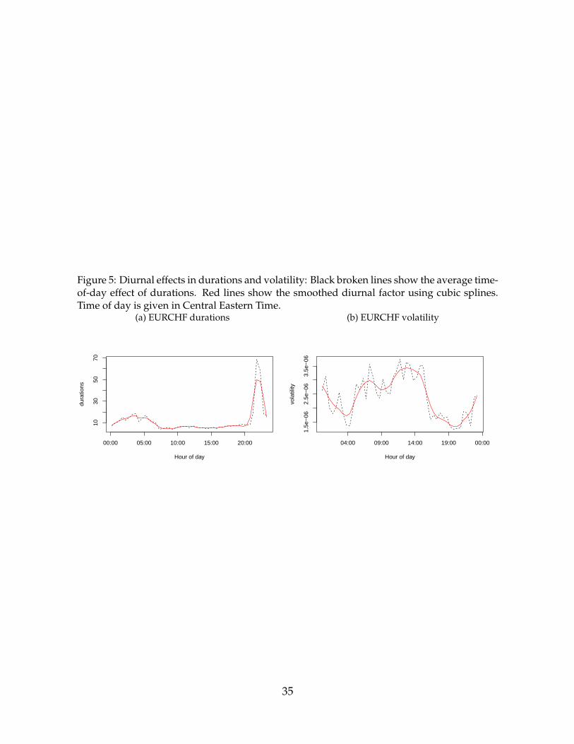
Figure 5: Diurnal effects in durations and volatility: Black broken lines show the average time-of-day effect of durations. Red lines show the smoothed diurnal factor using cubic splines.Time of day is given in Central Eastern Time.

(a) EURCHF durations

00:00 05:00 10:00 15:00 20:00

1030

5070

Hour of day

dura

tions

(b) EURCHF volatility

04:00 09:00 14:00 19:00 00:00

1.5e

−06

2.5e

−06

3.5e

−06

Hour of day

vola

tility

35

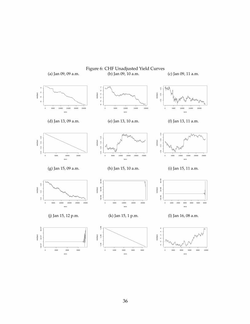
Figure 6: CHF Unadjusted Yield Curves(a) Jan 09, 09 a.m.

0 5000 10000 15000 20000 25000

−8

−6

−4

−2

secs

rate

(bps

)

(b) Jan 09, 10 a.m.

0 5000 10000 15000 20000

−6

−5

−4

−3

−2

−1

secs

rate

(bps

)

(c) Jan 09, 11 a.m.

0 5000 10000 15000 20000

−2.

5−

2.0

−1.

5

secs

rate

(bps

)

(d) Jan 13, 09 a.m.

0 5000 10000 15000

−2.

3−

2.2

−2.

1−

2.0

secs

rate

(bps

)

(e) Jan 13, 10 a.m.

0 5000 10000 15000 20000 25000

−2.

5−

2.0

−1.

5−

1.0

secs

rate

(bps

)

(f) Jan 13, 11 a.m.

0 5000 10000 15000 20000 25000

−2.

6−

2.2

−1.

8−

1.4

secs

rate

(bps

)

(g) Jan 15, 09 a.m.

0 5000 10000 15000 20000 25000

−2.

4−

2.2

−2.

0

secs

rate

(bps

)

(h) Jan 15, 10 a.m.

0 5000 10000 15000 20000

−6e

+98

−3e

+98

0e+

00

secs

rate

(bps

)

(i) Jan 15, 11 a.m.

0 1000 2000 3000 4000 5000 6000

−2e

+48

2e+

486e

+48

secs

rate

(bps

)

(j) Jan 15, 12 p.m.

0 2000 4000 6000

−2e

+27

2e+

276e

+27

secs

rate

(bps

)

(k) Jan 15, 1 p.m.

0 1000 2000 3000 4000

−1.

94−

1.90

−1.

86

secs

rate

(bps

)

(l) Jan 16, 08 a.m.

0 2000 4000 6000 8000 10000

−4

−2

02

46

secs

rate

(bps

)

36

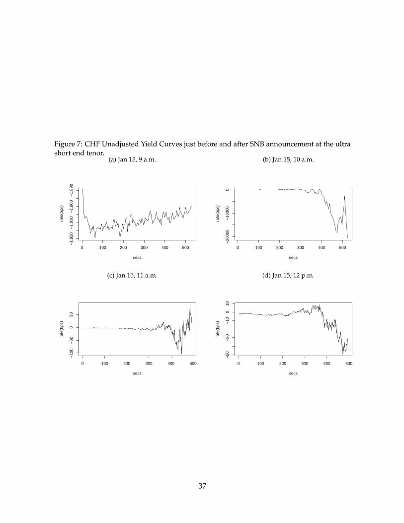
Figure 7: CHF Unadjusted Yield Curves just before and after SNB announcement at the ultrashort end tenor.

(a) Jan 15, 9 a.m.

0 100 200 300 400 500

−1.

920

−1.

910

−1.

900

−1.

890

secs

rate

(bps

)

(b) Jan 15, 10 a.m.

0 100 200 300 400 500

−20

000

−10

000

0

secs

rate

(bps

)

(c) Jan 15, 11 a.m.

0 100 200 300 400 500

−10

0−

500

50

secs

rate

(bps

)

(d) Jan 15, 12 p.m.

0 100 200 300 400 500

−50

−30

−10

010

secs

rate

(bps

)

37

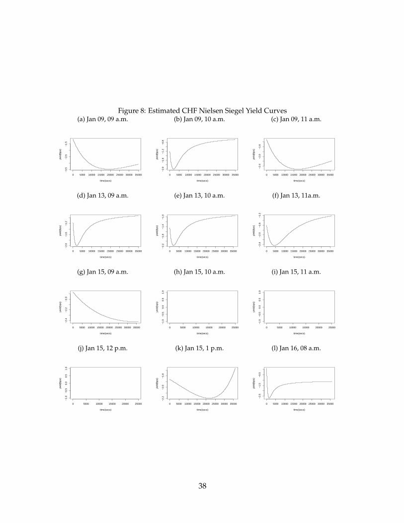
Figure 8: Estimated CHF Nielsen Siegel Yield Curves(a) Jan 09, 09 a.m.

0 5000 10000 15000 20000 25000 30000 35000

−3.

5−

2.5

−1.

5

time(secs)

yiel

d(bp

s)

(b) Jan 09, 10 a.m.

0 5000 10000 15000 20000 25000 30000 35000

−2.

0−

1.6

−1.

2−

0.8

time(secs)

yiel

d(bp

s)

(c) Jan 09, 11 a.m.

0 5000 10000 15000 20000 25000 30000 35000

−2.

4−

2.0

−1.

6

time(secs)

yiel

d(bp

s)

(d) Jan 13, 09 a.m.

0 5000 10000 15000 20000 25000 30000 35000

−2.

0−

1.6

−1.

2

time(secs)

yiel

d(bp

s)

(e) Jan 13, 10 a.m.

0 5000 10000 15000 20000 25000 30000 35000

−2.

2−

1.8

−1.

4−

1.0

time(secs)

yiel

d(bp

s)

(f) Jan 13, 11a.m.

0 5000 10000 15000 20000 25000 30000 35000

−2.

4−

2.0

−1.

6−

1.2

time(secs)

yiel

d(bp

s)

(g) Jan 15, 09 a.m.

0 5000 10000 15000 20000 25000 30000 35000

−2.

4−

2.2

−2.

0

time(secs)

yiel

d(bp

s)

(h) Jan 15, 10 a.m.

0 5000 10000 15000 20000 25000

−1.

0−

0.5

0.0

0.5

1.0

time(secs)

yiel

d(bp

s)

(i) Jan 15, 11 a.m.

0 5000 10000 15000 20000 25000

−1.

0−

0.5

0.0

0.5

1.0

time(secs)

yiel

d(bp

s)

(j) Jan 15, 12 p.m.

0 5000 10000 15000 20000 25000

−1.

0−

0.5

0.0

0.5

1.0

time(secs)

yiel

d(bp

s)

(k) Jan 15, 1 p.m.

0 5000 10000 15000 20000 25000 30000 35000

−2.

2−

2.0

−1.

8

time(secs)

yiel

d(bp

s)

(l) Jan 16, 08 a.m.

0 5000 10000 15000 20000 25000 30000 35000

−2.

5−

1.5

−0.

5

time(secs)

yiel

d(bp

s)

38

List of Tables

1 Descriptive statistics of returns and durations of intraday EURCHF FXdata during the period 08-16 January 2015. . . . . . . . . . . . . . . . . 40

2 Descriptive statistics of diurnally-adjusted returns and durations of EU-RCHF during the period 08-16 January 2015. . . . . . . . . . . . . . . . 41

3 Estimations for the log-ACD UHF-GARCH model for 9, 13, 15 and 16January 2015 for EURCHF using the last 1,000 observations at indicatedtimes. Both returns and durations used have been adjusted for intradaydiurnality. Standard errors for log-ACD are given in brackets. Robuststandard errors are used for UHF-GARCH and also given in brackets.† indicates significance at 5% or better. . . . . . . . . . . . . . . . . . . . 42

4 Nelson Siegel parameters estimated using nonlinear least squares. b0,the long run factor is constrained to the daily CHF O/N rate and notestimated, except during the flash crash period. Standard errors aregiven in brackets. † indicates significance at 5% or better. . . . . . . . . 43

39

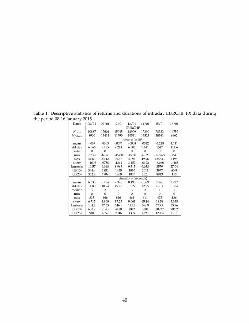
Table 1: Descriptive statistics of returns and durations of intraday EURCHF FX data duringthe period 08-16 January 2015.

Dates 08/01 09/01 12/01 13/01 14/01 15/01 16/01EURCHF

Nraw 10887 17604 15045 12909 17390 78333 14752Nfilter 8900 13414 11790 10541 13523 30361 6962

returns (×105)mean -.007 .0003 -.0071 -.0008 .0012 -6.228 4.141

std.dev 6.566 7.785 7.211 6.508 7.611 1517 111.6median 0 0 0 0 0 0 0

min -62.45 -62.45 -45.80 -45.80 -49.96 -123429 -1541max 41.63 54.12 49.96 49.96 49.96 125843 1198skew -.1649 .0758 .1364 .1450 .0192 -6.060 -.4165

kurtosis 10.57 9.048 8.963 9.315 9.038 3579 27.04LB(10) 344.4 1880 1455 1010 2011 3977 60.9LB(25) 352.4 1909 1468 1057 2020 8913 155

durations (seconds)mean 6.633 5.904 7.326 8.195 6.389 2.845 3.927

std.dev 11.80 10.94 19.02 15.27 12.75 7.614 6.524median 3 2 2 3 2 1 1

min 0 0 0 0 0 0 0max 335 166 816 461 611 473 136skew 6.715 4.900 17.25 9.061 15.44 18.58 5.338

kurtosis 104.3 37.55 546.0 175.3 548.9 765.7 53.96LB(10) 630.2 2548 4410 2812 3304 20237 906.2LB(25) 904 4552 7046 4339 4295 42984 1218

40

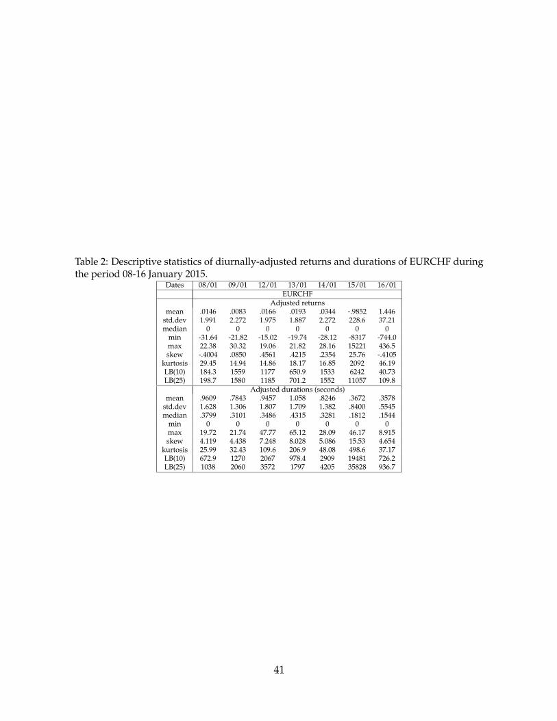
Table 2: Descriptive statistics of diurnally-adjusted returns and durations of EURCHF duringthe period 08-16 January 2015.

Dates 08/01 09/01 12/01 13/01 14/01 15/01 16/01EURCHF

Adjusted returnsmean .0146 .0083 .0166 .0193 .0344 -.9852 1.446

std.dev 1.991 2.272 1.975 1.887 2.272 228.6 37.21median 0 0 0 0 0 0 0

min -31.64 -21.82 -15.02 -19.74 -28.12 -8317 -744.0max 22.38 30.32 19.06 21.82 28.16 15221 436.5skew -.4004 .0850 .4561 .4215 .2354 25.76 -.4105

kurtosis 29.45 14.94 14.86 18.17 16.85 2092 46.19LB(10) 184.3 1559 1177 650.9 1533 6242 40.73LB(25) 198.7 1580 1185 701.2 1552 11057 109.8

Adjusted durations (seconds)mean .9609 .7843 .9457 1.058 .8246 .3672 .3578

std.dev 1.628 1.306 1.807 1.709 1.382 .8400 .5545median .3799 .3101 .3486 .4315 .3281 .1812 .1544

min 0 0 0 0 0 0 0max 19.72 21.74 47.77 65.12 28.09 46.17 8.915skew 4.119 4.438 7.248 8.028 5.086 15.53 4.654

kurtosis 25.99 32.43 109.6 206.9 48.08 498.6 37.17LB(10) 672.9 1270 2067 978.4 2909 19481 726.2LB(25) 1038 2060 3572 1797 4205 35828 936.7

41

Tabl

e3:

Esti

mat

ions

for

the

log-

AC

DU

HF-

GA

RC

Hm

odel

for

9,13

,15

and

16Ja

nuar

y20

15fo

rEU

RC

HF

usin

gth

ela

st1,

000

obse

rvat

ions

atin

dica

ted

tim

es.

Both

retu

rns

and

dura

tion

sus

edha

vebe

enad

just

edfo

rin

trad

aydi

urna

lity.

Stan

dard

erro

rsfo

rlo

g-A

CD

are

give

nin

brac

kets

.Rob

usts

tand

ard

erro

rsar

eus

edfo

rUH

F-G

AR

CH

and

also

give

nin

brac

kets

.†in

dica

tes

sign

ifica

nce

at5%

orbe

tter

.lo

g-A

CD

UH

F-G

AR

CH

ω1

α1

β1

γLL

LB

(10)

LB

(25)

ρ2

φ2

κ2

ω2

α2

β2

γ2

LLLB

(10)

LB(2

5)9

Jan,

9am

.051

1†.1

024†

.869

0†.9

211†

-951

.02

3.70

211

.94

-.007

8-.2

531

-.020

7†.0

884

.137

5.0

000

.890

3†-1

798.

1814

.10

22.4

9(.0

155)

(.025

8)(.0

581)

(.020

6)(.1

511)

(.159

1)(.0

095)

(.079

0)(.1

123)

(.036

8)(.1

632)

9Ja

n,10

am.0

763†

.141

8†.9

824†

.932

0†-8

59.6

414

.89

36.4

4.1

358

-.424

8†-.0

099

.000

0.1

125

.002

61.

247†

-195

2.41

11.0

020

.02

(.014

9)(.0

263)

(.019

5)(.0

208)

(.118

5)(.0

830)

(.008

1)(.0

000)

(.079

3)(.0

276)

(.145

7)9

Jan,

11am

.113

0†.2

290†

.881

0†.8

720†

-765

.79

10.5

424

.90

.000

6-.2

947†

-.007

6.0

000

.165

9†.0

000

1.02

2†-1

952.

4211

.36

23.8

5(.0

235)

(.031

6)(.0

400)

(.019

2)(.1

305)

(.128

2)(.0

055)

(.000

0)(.0

611)

(.076

7)(.1

622)

13Ja

n,9a

m.0

381†

.087

3†.9

796†

.994

0-7

50.1

04.

580

22.0

2.0

352

-.353

2.0

030

.104

3.1

489

.000

01.

055†

-194

4.55

18.9

242

.92

(.010

4)(.0

227)

(.018

0)(.0

222)

(.455

1)(.4

235)

(.015

5)(.2

573)

(.113

6)(.0

684)

(.197

6)13

Jan,

10am

.069

7†.1

190†

.957

2†.9

000†

-970

.80

7.32

421

.97

-.198

2-.0

680

-.009

3.1

622

.274

1.0

000

.519

1†-1

631.

7317

.83

45.7

3(.0

146)

(.023

0)(.0

251)

(.020

2)(.1

791)

(.217

8)(.0

092)

(.145

7)(.1

810)

(.073

2)(.1

597)

13Ja

n,11

am.0

541†

.105

5†.8

995†

.898

6†-9

11.8

74.

2333

23.9

1.2

050

-.440

4-.0

102

.254

0†.4

929†

.000

0.2

361†

-148

8.19

10.4

150

.48

(.015

0)(.0

237)

(.043

1)(.0

203)

(.543

9)(.4

438)

(.012

6)(.1

294)

(.243

2)(.1

109)

(.072

5)15

Jan,

9am

.071

3†.1

319†

.940

4†.9

236†

-950

.85

8.83

615

.33

.350

1†-.6

877†

-.000

9.0

036

.006

5.9

931†

.000

0-1

858.

9411

.26

25.6

2(.0

143)

(.022

8)(.0

245)

(.020

7)(.1

101)

(.082

3)(.0

119)

(.034

9)(.0

072)

(.000

8)(.0

166)

15Ja

n,10

am.0

604†

.093

7†.9

791†

.848

3†-9

87.9

510

.43

30.3

7-.1

663

-.146

2.0

151

.000

0.5

952†

.644

1†.1

764†

-382

8.15

131.

4527

4.0

(.012

1)(.0

176)

(.015

7)(.0

185)

(.142

9)(.1

376)

(.017

0)(.0

000)

(.116

2)(.0

387)

(.074

2)15

Jan,

11am

-.650

0†.3

890†

.570

0†1.

656†

861.

656.

995

23.8

2.7

270†

-.879

3†-.9

537

18.4

3.1

614†

.871

5†.0

000

-508

6.88

47.7

771

.60

(.156

6)(.0

454)

(.095

1)(.0

311)

(.238

3)(.1

663)

(3.8

70)

(87.

55)

(.048

0)(.0

430)

(7.4

92)

15Ja

n,12

pm-.1

900

.210

0†.8

270†

1.47

3†48

3.42

11.4

824

.25

.493

5†-.6

858†

-.108

49.

462

.090

5†.9

220†

.000

0-5

127

14.6

120

.13

(.120

1)(.0

382)

(.091

8)(.0

308)

(.160

1)(.1

252)

(1.0

20)

(153

.6)

(.038

0)(.0

329)

(32.

74)

15Ja

n,1p

m-.0

040

.085

2†.9

855†

1.49

5†50

4.81

9.29

024

.020

6-.1

243

1.07

1.0

000

.057

7.0

000

90.7

1†-4

464.

113.

109

20.4

0(.0

210)

(.019

8)(.0

153)

(.030

5)(.1

541)

(.149

9)(1

.618

)(.0

015)

(.050

4)(.4

13)

(43.

09)

16Ja

n,8a

m-.1

610†

.227

0†.6

880†

1.13

5†-1

97.7

14.9

720

.29

.965

9†-.9

330†

.241

218

.01

.066

0†.9

227†

.000

0-4

882.

297.

170

35.0

8(.0

821)

(.040

0)(.1

093)

(.024

2)(.0

245)

(.038

4)(.7

643)

(28.

98)

(.023

5)(.0

278)

(7.6

64)

42

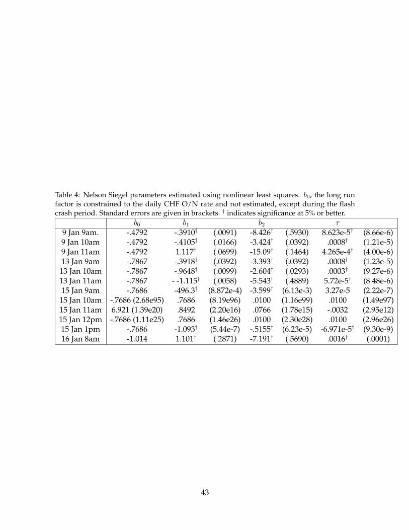
Table 4: Nelson Siegel parameters estimated using nonlinear least squares. b0, the long runfactor is constrained to the daily CHF O/N rate and not estimated, except during the flashcrash period. Standard errors are given in brackets. † indicates significance at 5% or better.

b0 b1 b2 τ9 Jan 9am. -.4792 -.3910† (.0091) -8.426† (.5930) 8.623e-5† (8.66e-6)9 Jan 10am -.4792 -.4105† (.0166) -3.424† (.0392) .0008† (1.21e-5)9 Jan 11am -.4792 1.117† (.0699) -15.09† (.1464) 4.265e-4† (4.00e-6)13 Jan 9am -.7867 -.3918† (.0392) -3.393† (.0392) .0008† (1.23e-5)

13 Jan 10am -.7867 -.9648† (.0099) -2.604† (.0293) .0003† (9.27e-6)13 Jan 11am -.7867 - -1.115† (.0058) -5.543† (.4889) 5.72e-5† (8.48e-6)15 Jan 9am -.7686 -496.3† (8.872e-4) -3.599† (6.13e-3) 3.27e-5 (2.22e-7)

15 Jan 10am -.7686 (2.68e95) .7686 (8.19e96) .0100 (1.16e99) .0100 (1.49e97)15 Jan 11am 6.921 (1.39e20) .8492 (2.20e16) .0766 (1.78e15) -.0032 (2.95e12)15 Jan 12pm -.7686 (1.11e25) .7686 (1.46e26) .0100 (2.30e28) .0100 (2.96e26)15 Jan 1pm -.7686 -1.093† (5.44e-7) -.5155† (6.23e-5) -6.971e-5† (9.30e-9)16 Jan 8am -1.014 1.101† (.2871) -7.191† (.5690) .0016† (.0001)

43