u~ ~1w~
TRANSCRIPT

II III 111111 1111 111111111111 1111 1111 111111 11111111 1111 11111111111
3 1176 00168 7889 I
, I
I .
NASA Technical Memorandum 83123
NASA-TM-8312319810019313
Two-boundary Grid Generation for the Solution of the Three-dimensional Compressible N avier-Stokes Equations
B. E. Smith
May 1981
NJ\5I\ National Aeronautics and Space Administration
Langley Research Center Hampton. Virginia 23665
FOR· REFERENCE -.;: , ............. ,"
JUN 29 1981
L~8i~/t~',', i'~'~12.\
li"\~'~PTryN: \~In~'~\".\
r '''~'''' "" ~ U~ ~1W~' "'" "" ""

LIST OF TABLES . .
LIST OF FIGURES LI ST OF SYMBOLS SUMMARY .... 1. INTRODUCTION. i •
2. ANALYSIS ..
TABLE OF CONTENTS
2.1 Navier-Stokes Equations of Motion.
2.2 Transformed Equations of Motion.
2.3 Definition of a Computational Domain and
Page
. . iii
v ix xv
1
6
7
• • • 10
Transformation Data . . . . 16
2.4 Two-Boundary Grid Generation . . . . 20
2.4.1 Approximate Boundary-Fitted Coordinate Systems Using Tension Spline Functions . 31
2.4.2 Transformation for a Wedge-Cylinder Corner. . 35
2.4.3 Transformation for a Spike-Nosed Body 48
2.5 Initial and Boundary Conditions ..... 61
2.5.1 Boundary Conditions for Supersonic Flow About Wedge-Cylinder Corners. . . . . . . . . . . 64
2.5.2 Boundary Conditions for Supersonic Flow About Spike-Nosed Bodies 68
3. COMPUTATIONAL ASPECTS 69
3.1 Computational Technique.
3.1.1 MacCormack Technique
. • • 71
. . . • 71
3.1.2 MacCormack Time-Split Technique. . . . . . . .. 74
3.2 Application of Vector Processing to the Computational Technique . . . . . . . . . . . . . . . . . . . . . . . 81

3.2.1 Vector Processing Using the CYBER 203 Computer . . . . . . . . . . . . . .
i i
Page
81
3.2.2 Program Organizational and Data Management. 82
4. RESULTS AND DISCUSSION . . . . . .
4.1 Supersonic Corner Flow Using Two-Boundary Grid Generation ........... .
4.1.1 High Resolution Grid Solutions ..
4.2 Supersonic Flow About Spike-Nosed Bodies
4.2.1 One-Half Inch Spike-Nosed Body ..
4.2.2 One and One-Half Inch Spike-Nosed Body.
5. CONCLUS IONS
REFERENCES
. . . .
88
89
108
130
131
144
149
152

Table
2
3
iii
LIST OF TABLES
Page
Data description for an airfoil grid . . . . . . . . .. 36
Data description for an one-half inch spike-nosed body
Data description for a one and one-half inch spike-nosed body .. . . . . . . . . . . . . . . . . . . . . • . .
59
60


v
LIST OF FIGURES
Figure
1. Computational domain
Page
17
2. Boundary mapping from the computational domain to the physical domain 23
3. Grid control function 29
4. Boundary definition for a Kc1nnan-Trefftz airfoil 37
5. Grid for a Karman-Trefftz airfoil obtained with the "two boundary techni que" .. ... 38
6. Three-dimensional corner geometries. . . . . . 39
7. Projection of a wedge onto the x-y plane and cross section of a grid in the y-z plane .. . . . . . 41
8. Grids for wedge-plate and wedge-cylinder corners at x/xL = 1.' . . . . . 44
9. One-hal finch spi ke-nosed body 49
10. One and one-half inch spike-nosed body 50
11. Grid generated with "t\'Io-boundary technique" for a one-half inch spike-nosed body .......... 57
12. Grid generated with the "two-boundary technique" for a one and one-half inch spike-nosed body 58
13.
14.
Flowchart for the Navier-Stokes solver
Vector arrangement in planes
15. Data management for the Navier-Stokes solver
16. Two-dimensional solutions
17. Physical dimensions of corners
18. Three-dimensional corner flow characteristics
19. Flow field description for a rectangular corner
20. Flow field description for a wedge-plate corner
85
86
87
92
93
94
99
100

Figure
21. Flow field description for a 12.20 wedge-plate corner . . . . . . . . . . . . . . . .
22. Flow field description for a plate-cylinder corner. .
23. Flow field description for a 60 wedge-cylinder corner. . . . . . . . . . . . . .
24. Flow field description for a 12.20 wedge-plate
25. Flow field description for an 180 wedge-plate corner . . . . . . . . . . . . . . . . .
26. Flow field description for an 180 wedge-plate corner (high Reynolds number) ....
27. Surface pressure for 180 wedge-plate corner
28. Surface pre~~ure for wedge-plate corners ...
29. Surface pressure for wedge-cylinder corners
30. Hypothetical symmetric corner flow from Ref. 37
31. Flow field solution for a 12.20 wedge-wedge corner . . . . . . . . . . .
32. Line contour plot of density for a 12.20
symmetric corner ........... .
33. Surface distribution of density - two views -12.20 symmetric corner ........ .
34. Surface pressure for a 12.20 symmetric
35.
36.
corner ..
Flow field description for a 12.20 asymmetric corner (12 x 64 x 64 grid-exact boundaries)
Line contour plot of 12.20 asymmetric corner (12 x 64 x 64 grid-exact boundaries) ....
. . .
37. Perspective view of distribution of density for 12.20
asymmetric corner x/xL = .8 (12 x 64 x 64 grid-exact boundaries) ..................... .
. . .
vi
101
102
103
104
105
106
107
109
110
112
115
116
117
118
121
122
123

Fi gu re
38. Surface pressure for a 12.20 asymmetric corner (12 x 64 x 64 grid-exact boundaries) ..... .
39. Surface pressure comparison for grid refinement at Re = 291994/m .............. .
40. Flow field description for a 12.20 asymmetric corner (12 x 64 x 64 grid-approximate boundaries)
41. Line contour plot for a 12.20 asymmetric corner (12 x 64 x 64 grid-approximate boundaries) ...
42. Perspective view of distribution of density for a 12.20 asymmetric corner x/xL = .8 ..... .
· · ·
· · ·
· · ·
· · · 43. Comparison of surface pressure for two-different grids
44. Development of density solution for a one-half inch spike-nosed body ................ .
45. Grid lines for. quantative comparison one-half inch spike-nosed body. . ..... .
46. Density along line one for base case
47. Density along line twenty-nine for base case
48. Density along line fifty-three for base case
49. Comparison of density solution for grid concentration change line = 1.
50. Comparison of density solution for grid concentration
vii
Page
· · 124
· • 125
· 126
· · 127
· · 128
• 129
· 133
· 134
· . 135
· 136
137
138
change line = 29 . . . . . . . . . . . . . . . . . .. 139
51. Comparison of density solution for grid concentration change line = 53 . . . . . .. ...... . . 140
52. Comparison of density solution for outer boundary change 1 ine = 1 ..................... 141
53.
54.
Comparison of density solution for outer boundary change line = 29
Comparison of density solution for outer boundary change line = 53 ....
142
· . 143
viii
Figure
55. Shadowgraphs of an oscillating flow field . . . . . 145
56. Density distribution during one cycle of oscillation for a one and one-half inch spike-nosed body. . . . 147
57. Surface pressure on one and one-half inch spike-nosed body ........ . 148

B
c 00
e
F,G,H
g",h" -+-+.,jo-i ,j ,k
LIST OF SYr1BOLS
parameter governing grid concentration for spike-nosed body grids
intermediate variables used in computing the pressure on a cylinder surface for wedge-cylinder corner meshes
specific heat at constant volume
specific heat at constant pressure
free stream speed of sound
intermediate variables used in computing pressure on a wedge surface for \.,.edge-cyl inder corner meshes
interna 1 energy
vector fluxes for coordinate directions
symbol· for flux vectors in a compact definition of the equations of motion
basis functions for cubic connecting function
second derivatives for tension spline approximation
unit vectors in the physical coordinate system
Jacobian matrix
inverse Jacobian matrix
determinant of inverse Jacobian matrix
magnitude of normal vector on bounding surfaces
coefficient of heat conduction
parameters governing the grid concentration for wedgecyl inder grids
parameters governing the grid concentration for spikenosed body grids
parameter governing the grid concentration for planar intersecting corner grids
ix

-k
L
M
M 00
m,n
N
N p
q
R
R =Re e 00
s
s,t
S
T
parameter governing grid concentration for planar intersecting corner grids
characteristic length
number of points describing the inside boundary for spike-nosed body grids
free stream Mach number
number of points describing boundaries for tension spline approximation
number of points in tension spline approximation
normal direction
pressure
heat conduction vector
components of heat conduct vector
radial direction
cylinder radii for wedge-cylinder grid description
radius of circle describing the outside boundary for spike-nosed body meshes
free stream Reynolds number
parametric variable for an airfoil grid
parametric variables
Sutherland viscosity law constant
four-dimensional array containing state variables and transformation data
temperature
reference temperature for Sutherland viscosity law
time
x

u
u,v,w -u
-v
parametric variable for inner boundary of spike-nosed body meshes
vector of state variables
velocity components in the physical domain
velocity vector
velocity used in computing time step for the finite difference technique
xi
X(),Y(),Z(),} functions relating the computational domain to the x(),y(),z() physical domain
x,y,z
x,y
x,y
-a
y
Yx,Yy'Yz
L'I~,L'ln,L'lZ;:
~t
8
functions relating the computational domain to the physical domain with boundary parameterization and third independent variabl e "connecti ng functi on"
coordinates for the physical domain
symbols for coordinates in the compact definition of the equations of motion
coordinates for the inside boundary of spike-nosed body grids
physical coordinate position in windward direction for the initial solid surface in wedge-cylinder corner grids
physical coordinate in the windward direction for the final grid plane in the wedge-cylinder corner grids
coefficient for pressure damping
ratio of specific heats
directional cosines of the normal vector at a solid wall
constant increments in the computational coordinates
increment in time
angle defining a parametric variable for the outside boundary of spike-nosed grids
angles defining boundaries of wedge cylinder corner grids

p
a
T
c/>X'c/>y'c/>Z
\}Jl,\}J2
Subscripts:
B
W
00
xii
angles defining boundaries of planar intersecting corner grids
intermediate angle for computing pressure boundary condition for wedge-cylinder corner grids
molecular viscosity
reference viscosity in Sutherland viscosity law
bulk viscosity
coordinates in the computational domain
redistributed coordinates relative to the computational domain
density
tension parameter
stress tensor
wedge angle for wedge-cylinder corner grids
angle of rotation for three-dimensional spike-nosed grids
components of viscous dissipation function
intermediate angles for wedge-cylinder grids
boundary value
solid wall value
free stream value

Superscripts:
I
o
Indices:
I,J,K,L
i ,j ,k
Opera tors:
o
a
inside boundary for spike-nosed body grids
outside boundary for spike-nosed body grids
indices used in four-dimensional S array
point indices
boundary indicator
gradient operator
inner product operator
finite difference operators
linear interpolation operator
partial differentiation
xiii


SUMMARY
TWO-BOUNDARY GRID GENERATION FOR THE SOLUTION OF THE THREE-DIMENSIONAL COMPRESSIBLE
NAVIER-STOKES EQUATIONS
Robert Edward Smith
xv
A grid generation technique called the IItwo-boundary technique ll is
developed and applied for the solution of the three-dimensional com
pressible Navier-Stokes equations describing laminar flow. The Navier
Stokes equations are presented relative to a xyz cartesian coordinate
system and are transformed to a ;ns computational coordinate system.
The grid generation technique provides the Jacobian matrix describing
the transformation.
The "two-boundary technique" is based on algebraically defining
two distinct boundaries of a flow domain and joining these boundaries
with a IIconnecting function" which is proposed to be linear or cubic
polynomials. The algebraic boundary representation can be analytical
functions or numerical interpolation functions. Control of the distri
bution of the grid in the physical domain is achieved by embedding "con
trol functions" which redistribute the uniform grid of the computational
domain and concentrate or disperse the grid in the physical domain. The
computer program to solve the Navier-Stokes equations is based on a
MacCormack time-split technique and is specifically designed for the
vector architecture and virtual memory of the CYBER 203 computer. The
program "Navier-Stokes solver" is written in the SL/l language which
allows 32-bit word arithmetic operations and storage. The program can
run with 5 x 10⁴ grid points using only primary memory, and the compu
tational speed is 4 x 10⁻⁵ seconds per grid point per time step.
Using the "two-boundary technique," grids are developed for two
distinctly different flow field problems, and compressible supersonic
laminar flow solutions are obtained using the Navier-Stokes solver.
Grids and solutions are obtained for a family of three-dimensional
corners at Hach number 3.64 and Reynolds numbers 2.92 x 10⁵/m and
3.9 x 10⁶/m. Also, grids are derived for spike-nosed bodies, and solu
tions are obtained at Mach number 3 and Reynolds number 7.87 x 10⁶/m.
Coupled with the Navier-Stokes solver, the "two-boundary technique"
is demonstrated to be viable for grid generation associated with com
puting supersonic laminar flow. The technique is easy to apply and is
applicable to a wide class of geometries. The "two-boundary technique"
can serve as the foundation for generating grids with highly complex
boundaries and yield grid pOint distributions that can capture rapidly
changing variables in a flow field.
xv;

1
1. INTRODUCTION
In recent years, the availability of large scale scientific com-
puter systems has resulted in rapid progress in the field of Computa
tional Fluid Dynamics. There is now the capability to calculate many
complex unsteady two-dimensional and steady three-dimensional flows.
MacCormack and Lomax [1]* summarize the "state of the art" for the
computation of compressible viscous fluid flow. For a heat conducting
compressible fluid acting near body surfaces with large separation
regions or inviscid-viscid interactions, the numerical solution of the
Navier-Stokes equations is the preferred approach [1]. An emerging
problem, however, i~ the generation of grid systems on which solutions
can be obtained when there are complex boundary geometries. This prob
lem is compounded in three dimensions. This study addresses the solu
tion of the three-dimensional compressible Navier-Stokes equations,
the generation of grids, and the solution algorithm-computer relation
ship. The emphasis is placed on grid generation.
An algebraic grid generation technique applicable to the Navier
Stokes equations is developed, and a three-dimensional Navier-Stokes
solver (compressible laminar flow) based on a proven numerical tech
nique (MacCormack time-split algorithm [1-4]) is developed for the CDC
CYBER 203 vector computer [5]. Also, flow visualization techniques have
been developed in conjunction with this research but will not be dis
cussed in detail. In order to evaluate the overall system for computing
viscous compressible flow, and in particular the grid generation *The numbers in brackets indicate references.
technique, grids are determined for a family of three-dimensional
corners and two spi ke-nosed bodi es ..
2
The gri d generation technique is called the "two-boundary tech
nique." It is applicable in two and three dimensions and is a method
ology for direct computation of the physical grid as a function of a
uniform rectangular computational grid. The Jacobian matrix of the
transformation can be obtained by direct analytic differentiation. This
is in contrast to the indirect approach where an elliptic partial dif
ferential equation system is solved for the coordinates of the physical
grid relative to the computational grid, and in which the Jacobian
matrix must be obtained by numerical differentiation. The indirect
approach is popularly known as the ITH4method" [1,6-10]. In the
"two-boundary technique, II two separate non-intersecting boundaries are
defined by means of algebraic functions or numerical interpolation
functions. These functions have as independent variables, coordinates
which are normalized to unity. Another function with an independent
variable defined on the unit interval connects the boundaries.
The "two-boundary technique" is based upon concepts found in the
theory of surface definition [11,12]. Gordon and Hall [13] postulate
the essentials of the technique and emphasize finite element grids.
Also, Eiseman [14-16] uses a form of the technique in generating grids
for multiconnected two-dimensional domains. In this investigation the
"two-boundary technique" is developed and is analyzed for finite differ
ence solutions for fluid flow applications. Low order polynomials
(linear and cubic) are used for connecting functions. For the cubic

3
connecting function, orthogonality can be enforced at the boundaries
through knowledge of the normal derivatives there. Control of the grid
(grid spacing in the physical domain) is achieved by the superposition
onto the independent variables algebraic or transcendental functions
with desirable characteristics. Splines under tension [17-19J are pro
posed for approximate boundary defi nition. The II two-boundary techni que"
is used to algebraically generate grids for a family of three-dimensional
corners and to generate a combined algebraic-numeric grid for spike
nosed bodies. The derivatives composing the Jacobian matrix for the
three-dimensional corners and spike-nosed bodies are presented for
obtaining numerical solutions of the Navier Stokes equations.
The CDC CYBER 203 is a large scale computer with vector processing
architecture and virtual memory. Generally efficiency using a vector
computer increases with increasing vector length, however, considerable
attention must be given to the algorithm-machine architecture relation
and balancing the vector length with practical limits of primary memory.
A MacCormack time-split solution algorithm is programmed for the
CYBER 203 computer and is called the "Navier-Stokes solver." The
MacCormack technique is used because of its robustness and adaptability
to vector processing. Another primary consideration when developing a
"Navier-Stokes solver" on a large complex computer is the capability to
solve a wide class of problems with a minimum of programming changes.
This has been accomplished by programming the complete transformed
equations of motion and storing all nine elements of the Jacobian
matrix of the transformation at each grid point (transformation data).

4
Supplying the transformation data from a grid generation technique and
programming the boundary conditions "for a given problem (separate sub
routine) allows the program be applied to virtually any laminar fluid
flow problem. Since the split MacCormack technique is used, two
dimensional solutions can be obtained without unnecessary computations.
The operator for the third dimension is bypassed. A final important
point relative to the Navier-Stokes solver is that the MacCormack tech
nique is written in the SL/l language [20J and uses the 32-bit arithmetic
option of the CYBER 203. By using 32-bit words, twice the in-core stor
age is available and approximately twice the computational speed is
achieved compared to the use of normal 64-bit words. There are approxi
mately two million words of primary memory and the computational speed
is 4 x 10⁻⁵ seconds per grid point per time step for the 32-bit word
length. For the explicit technique, no significant degeneration in
accuracy is observed using the smaller word size. The Navier-Stokes
solver is independent of the grid generation technique, and the trans
formation data from any technique can be used by the code.
Using the IItwo-boundary technique ll grids are developed for two
distinctly different flow field problems, and compressible supersonic
laminar flow solutions are obtained using the computer program based on
the MacCormack technique. A set of algebraic grid generation equations
are developed using the IItwo-boundary technique ll for a family of three
dimensional corners consisting of wedge-cylinder, plate-cylinder,
approximate wedge-plate, and approximate rectangular corners. It is
also shown that exact grids for planar intersecting corners can be
5
derived with the "two-boundary technique." Corner flow solutions are
obtained on a 20 x 36 x 36 grid and a 12 x 64 x 64 grid. The solutions
obtained on the 12 x 64 x 64 grid are compared with physical experiments
and other numerical experiments. The Mach number used is 3.64 and the
Reynolds number is 2.92 x 10⁵/m and 3.9 x 10⁶/m.
Also, algebraic grids are derived using the "two-boundary technique"
for spike-nosed bodies. In particular, grids for a one-half inch spike
nosed body and a one and one-half inch spike-nosed body are obtained.
Supersonic flow solutions at Mach number 3 and Reynolds number
7.87 x 10⁶/m are obtained about these configurations. Unlike the flows
about the three-dimensional corners, the flow about the spike-nosed
bodies is unsteady. The amplitude of the oscillations about the one-half
inch nose body is quite small, however, the one and one-half inch spike
nosed body flow field oscillates with a large amplitude. The high
amplitude solutions are compared with physical experiments. The flow
fields are two-dimensional axisymmetric, but are solved with a three
dimensional Navier-Stokes solver resulting in considerable savings of
development time for a specialized axisymmetric code.
For flow visualization. a relatively novel approach has been
developed where a color spectrum is used to display a scalar variable
such as density, Mach number, etc •• on a two-dimensional slice of a flow
field. Sequences of pictures can show the history of a developing flow
or a scan of the flow field in a three-dimensional domain. The Diccomed
Digital Display/Film Writer system which is normally used for environ
mental image processing is used for the flow visualization.

6
In summary, the main objectives of this study are the development
of an algebraic grid generation procedure, the development of software
to solve the compressible three-dimensional Navier-Stokes equations on
a vector computer using the results of the grid generation technique,
and the application of the grid generation technique and software to
solve specific supersonic flow problems. The organization is as
follows. In Chapter 2 the three dimensional compressible Navier-Stokes
equations are presented relative to a Cartesian coordinate system and
are transformed to a uniform grid computational coordinate system.
This introduces the information that must be determined by the grid
generation technique. The "two-boundary technique" is developed and
applied to generate grids and Jacobian derivatives for a family of
three-dimensional corners, spike-nosed bodies, and an airfoil configura
tion. In Chapter 3, the MacCormack technique is presented, and its
compatibility with the CYBER 203 is described. In Chapter 4, supersonic
flow solutions about three-dimensional corners and spike-nosed bodies
obtai ned with the "two-boundary technique" and Navi er-Stokes solver
are described.
2. ANALYSIS
This chapter develops the equations of motion and the "two
boundary technique" for grid generation. Grids and boundary conditions
are developed for a family of three-dimensional corners and for spike
nosed bodies. Also, grids are developed for airfoil boundaries using
splines under tension.

7
2.1 Navier-Stokes Equations of Motion
The governing equations which describe the motion of a viscous
compressible heat conducting fluid are the continuity equation, momen
tum equations, and energy equation. These'equations are derived from
the concept of continuum mechanics. The continuum concept and deriva
tion of the Navier-Stokes equations of motion are found in several
references, of which Schlichting [21] is the most notable.
Expressed in symboic form the Navier-Stokes equations of motion
are:
Continuity: .£Q. + 'V at . (pUJ = 0, (2.1a)
Momentum: a(pu) + 'V • (puu at - T) = 0, (2.1b)
Energy: a(pe) + 'V • (peu + q - U • T) 0. (2.1c) at =
The stress tensor, dissipation function, and heat conduction for a
rectangular cartesian coordinate system are:
TXX Txy TXZ
T = Txy Tyy Tyz - stress tensor
TXZ Tyz TZZ
where
T = _p + 21I~ + (.' 2) (au + av + aw) xx ax liB - Jll ax ay dZ'
.. " ~

and
T = _p + 211 aV + (llQ _ Jll2 ) (E.!! + av + aWl yy ay I-' ax ay az
_ (au + av) T xy - II ay ax'
_ (aw + au) TXZ - II ax az'
_ (av + aWl Tyz - II az ay'
<P = X
U . T = <P = y
<P = Z
-aT q = -K-x ax
. -aT q = q = -K-y ay
-aT q= -K-z az
UTxx + VTxy + WTXZ
UT + VT + WT xy yy yz - dissipation
UTXZ + VTyz + WTZZ
- Heat flux vector,
8
function,

9
The viscosity coefficient ~ is a function of temperature and is
adequately approximated by Sutherland's semiempirical equation:
with
The bulk viscosity coefficient ~S is set equal to zero. This is
a reasonable assumption for a monatomic gas where the molecules has no
internal degree of freedom. For a polyatomic gas the bulk viscosity is
not always zero and can be the same order of magnitude as the molecular
viscosity in sound propagation and shock structure. A detailed discus
sion of bulk viscosity is given by Vincenti and Kruger [22].
At this point there are five coupled partial differential equations
and one algebraic equation with eight .unknowns: p, u, v, w, P, e,
T, and ~. In order to have a complete system, there must be two addi
tional equations relating the unknowns. The equation of state is
P = P (p,T),
and for a perfect gas P = pRT and e = CVT where Cv is the specific
heat at constant volumn, and R is the gas constant. For compatible
boundary conditions this system of equations is solvable.

10
2.2 Transformed Equations of Motion
The equations of motion in Section 2.1 are expressed in terms of a
Cartesian coordinate system. If an object is defined in this coordinate
system and a flow is to take place about the object, it is desirable to
perform the computation in a coordinate system which conforms to the
boundaries of the object. There are two primary reasons for wanting the
coordinate system to be boundary-fitted. Boundary-fitted coordinates
afford the ability to apply boundary conditions exactly avoiding inter
polation error, and they minimize the logic that is necessary to apply
boundary conditions. The penalty for these advantages is added com
plexity of the equations of motion. Another consideration is that when
the domain of the flow field is discretized, it is desirable to have
grid points concentrated in certain regions where high rates of change
are likely to occur. For instance, in the boundary layer region more
grid points are necessary to resolve the rapid change in the state
variables. If the cartesian coordinate system where the object is
defined is called the physical domain, the coordinate system relative
to the boundaries of the object is called the computational domain. The
relationship between the physical domain and the computational domain is
a unique single-valued transformation with continuous derivatives such
that if the coordinates in the computational domain are ~, n, ~:
then
~ = ~(x,y,z), n = n(x,y,z), and ~ = ~(x,y,z).

11
Conversely,
where x, y, and z are coordinates in the physical domain. Since
the equations of motion in terms of the Cartesian coordinate system of
the physical domain are advantageously solved in terms of the coordinate
system of the computational domain, the equations must be transformed.
This is accomplished by expressing the derivatives of the state variables
with respect to the xyz components of the physical domain in terms of
the ~ns components of the computational domain as follows:
au ax
av ax
aw ax
au ay
av ay
av az
aw az
=
au a~
av ~
au an
av an
aw an
aw ~
Notice that u, v, and ware the velocities along the x, y,
and z axes in the physical domain.

-.
,(~e xe lle Xe je Xe ~e Ae lle Ae he ""5€ + Ae 1l€ + Ae ~ + ne ""5€ + ne LLe + je Ae) rt = AX~ ne je
\
, (~e Ze lle Ze je ze \ Me 3€ + Me LLe + Me ~ +
~e A'e "e A'e ,e A'e ~e xe "e xe ,e xe) Ae "3€ + Ae lle + Ae ~ + ne 3€ + ne lle + ne ~ rt £/2
(~.!:!l "e ze 'e.!:!l \ rtz d- _ zz, Me ~e ~ Me lle + Me je I + -/
, (~e ze lle ze je ze Me "3€ + Me lle + Me ~ +
~e Ae lle Ae je Ae ~e xe lle xe je xe) Ae "3€+Ae LLe+he ~+ne 3€+ne LLe+ne ~ rt £/2
(~e Ae lle Ae je Ae) AA Ae "3e + Ae lle + J\e je rt2 + d - = ~
I
, (~e ze "e ze ze ze Me ]e + Me TIe + Me 3e +
~e Ae lle Ae je Ae ~e xe lle xe je . xe\ J\e 1e + he LLe + he 3e + ne "3€ + ne Ue + ne je J rt £/2 -
(~e ~ lle ~ je xe) rt __ xx~ \ne ~e + ne lle + ne je 2 + d -
:sawoJaq ~osual ssa~ls a4l saLqe~~eA paw~oJsue~l a4l JO sw~al UI
2L

ze te xe "5e 3€ 3€
I~ te xe ~osua+ ~ap~o puoJas a4I r = lie lie lie -
ze te xe ~ :3e ~.
. (:ie ze lie ze Ie 3€ + Ie lie
:3e ze) + Ie :3e
, (:ie te lie te :3e te) Ie 3e + Ie lie + Ie ~
)f = zb
)f = tb •
'(:ie xe + lie ~ + E ~) )1_ = xb Ie:ie Ie lie Ie:3e - •
put?
:sawoJaq uO~+JnpuoJ +t?a4 a4I
. (:ie te + lie te + E. te ~ ~ lIeze :3e ze\ rt zt \Me:ie Me lie Me:3e + Ae :ie + A€ lie + A€ :3e) = J.
put?
'(:ie ze ~ ~ E. ~ ~ ~ lie El + ~ xe) rt = zXJ. ne ~ + ne lie + ne :3e + Me :ie + Me lie Me:3e
£L

14
is called the Jacobian matrix of the transformation whose elements are
the nine derivatives specifying the" rate of change of the computational
coordinates with respect to the physical coordinates. The equations of
motion (Eq. (2.1)) are in conservation form [3J and can be expressed as
E.!! + aF + aG + aH = a at ax ay az ' (2.2)
where
pu p
puu - T pu xx U = pv F = puv - T xy
pw Puw - T pe xz
peu + q - 4> . x . x
pv pw
puv - Txy puw - TXZ G = pvv - Tyy H = pvw - Tyz
pvw - TXZ pww - TZZ . pev + q -y <P' Y
pew + qz - 4>z
15
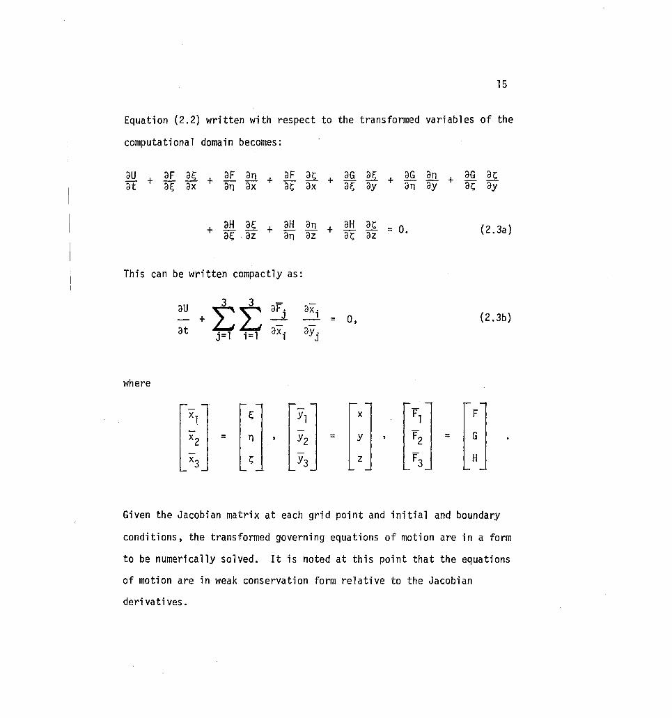
Equation (2.2) written with respect to the transformed variables of the
computational domain becomes:
au + aF a~ + aF E.!l + aF ~ + aG a~ + aG an at ~ ax an ax ~ ax ~ ay an ay
+ aH a~ + aH an + a~ az an az
This can be written compactly as:
3 3
aH az;; = ~ az o.
au + L:L: ax. 1 = 0,
at j=l i=l ay. J
where
xl ~ Yl x
x2 = n Y2 = Y
x3 z;; Y3 z
F,
F2
F3
aG az;; + ~ ay
{2.3a}
(2.3b)
F
= G
H
Given the Jacobian matrix at each grid point and initial and boundary
conditions, the transformed governing equations of motion are in a form
to be numerically solved. It is noted at this point that the equations
of motion are in weak conservation form relative to the Jacobian
derivatives.

16
2.3 Definition of a Computational Domain and Transformation Data
In the previous section the Navier-Stokes equations are transformed
from a Cartesian coordinate system to a computational domain. In so
doing nine additional unknowns, which are the elements of the Jacobian
matrix, are added to the problem. When the finite difference technique
described herein is applied to Equation (2.3), the Jacobian matrix
must be known at each grid point. The objective of a grid generation
technique is to provide the Jacobian matrix which is henceforth called
transformation data. The computational domain is defined in this sec
tion along with the formulas necessary for computing the transformation
data based on known functional relations between the computational domain
and the physical domain. The next three sections concentrate on deter
mining functional relations between the computational and physical
domains. The computational domain is defined to be a rectangular
parallelepiped and a uniform grid is superimposed onto the domain
(Fig. 1) such that:
!::J.E., = constantl ,
!::J.n = constant2,
!::J.7;, = constant3•
(2.4)

17
n
t lin
t
VVVVVLLVVVVV//// VVVVVVVVLLLLL///V VVVVVVVVVVVVVVVC~~
VVVVVVVVVVVVV/VV VVV//VVVVVVVVVVVV~VV
VVVVVVVVVVVVVVVVVV VV VVVVVVV/////////VVV~V~
VVV//VVV/L/VVVVVVVVV V VVVVVVVVV/L//L//VVVVVVVV ////////////////VVVVVVV~~
VVVVV~~~VY ~VV~~VVVVI/ V~~VVVvvvv I/VVVVVVVVV V~VVV~~~~V VVVV~V v ~V~~VV~ VVVVl/V/ vVVVL V V ~TlI~ V V VV
.V -11-
1Ir,
\£.------r,
Fi g . . 1 Computational domain. ~ - .. .-

18
A fUnctional relation between the computational domain and the physical
domain can be expressed as
Further, these functions must map boundaries in the computational
domain onto boundaries in the physical domain such that
(2.5)
where xB' YB and zB define the boundaries of the physical domain
and ~B' nB' and ~B define the boundaries of the computational
domain. The transformation data is composed of the rates of change of
the computational coordinates with respect to the physical coordinates.
If the inverse functional relations
~ = ~(x,y,z), n = n(x,y,z), and ~ = ~(x,y,z) (2.6)
are known, the transformation data can be directly found by differ-
entiation. It is not necessary, however, to know the inverse functional
relations to determine the transformation data. The Jacobian matrix
can be evaluated by differentiating the functional relation (Eq. (2.5)).
That is
r ax a~
ax ax an a~
J-1 = ~ a~
~ ~ an a~
az az az ~ an ~

19
and then
J = Transposed of Cofactor (J-') I J-'I '
-, where IJ I is the Jacobian determinate and J-1 is the inverse
Jacobian matrix.
ax ax ax at,; an as
IJ-'I = ~ ~ ~ at,; an as
az az az ~ an ~
= ax (~ az ~ ~) ax (~ az ~ ~) ~ - - an at,; an as an at,; as as at,;
+ ax (~ az ~ ~) -as at,; an an at,;
and
-, at,; at,; at,; ax ax ax ax ay az a~ an ~
an an an = J = ~ ~ ~ ax ay az at; an as
as as as az az az ax ay az at,; an ~

_(~~ _ ~ OZ) oF; or;; or;; ol;
(~~-~~) ol; on on ol;
-(~~-~~) on 01'; 01'; on
(ox oZ _ ~~) oF; 01'; 01'; oF;
_(ox ~ _ AX OZ) ol; on on ol;
-(~~-~~) aF; ar;; or;; ol;
(~~ _ OX~) ol; on on ol;
20
(2.7)
provided IJ- l I r O.
The transformation data can be pre-evaluated and stored or it can
be computed as needed. The trade off is the additional computation
cost versus the storage cost. For the Navier-Stokes solver discussed
in this study, the transformation data is precomputed and stored for
later use.
2.4 Two-Boundary Grid Generation
A computational domain is postulated by Equation (2.4). It is a
rectangular parallelpiped in three dimensions and a square in two
dimensions. The physical domain is a subdomain of a Cartesian coordi
nate system. A transformation between the physical domain and the com
putational domain is a mathematical relationship mapping one domain
onto the other. Similarly a grid in one domain is mapped onto a grid
in the other domain. When the transformation maps boundaries in the
physical domain onto boundaries in the computational domain the term
"boundary-fitted coordinate system" is used to describe the
transformation.
21
An indirect (differential) approach for finding the relationship
between the computational and physical grids described by Thompson
et al. [6-10] has been highly successful. In this approach the
elliptic system of partial differential equations which must be satis
fied by the mapping between the two domains is numerically solved by an
iterative technique such as Successive-Over-Relaxation (SOR). The
numerical solution is the grid in the physical domain corresponding to
the grid in the computational domain. The transformation data is
obtained by numerical differentiation, and a grid change requires a
new solution of the elliptic system.
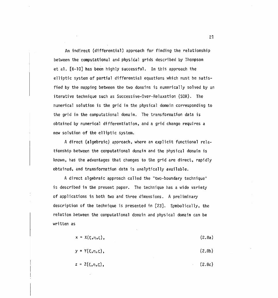
A direct (algebraic) approach, where an explicit functional rela
tionship between the computational domain and the physical domain is
known, has the advantages that changes to the grid are direct, rapidly
obtained, and transformation data is analytically available.
A direct algebraic approach called the IItwo-boundary technique ll
is described in the present paper. The technique has a wide variety
of applications in both two and three dimensions. A preliminary
description of the technique is presented in [23]. Symbolically, the
relation between the computational domain and physical domain can be
written as
x = X(l=;,n,z;),
y = Y(i;,n,z;;),
z = Z(i;,n,z;),
(2.8a)
(2.8b)
(2.8c)

O~~~l,
O~n~l,
O~r;~l.
22
Equation (2.8) is equivalent to Equation (2.5). For a boundary-fitted
relationship between the two domains, boundaries in the computational
domain should map onto boundaries in the physical domain as shown in
Figure 2. For instance, for the boundaries n = 0 and n = 1 in the
computation domain, Equation (2.8) becomes
Xl = X(~,O,r;) = Xl(~,r;),
Yl = y(~,O,r;) = Yl(~,r;),
zl = Z(~,O,r;) = Zl(~,r;),
x2 = X(~,l,r;) = X2(~,r;),
Y2 = y(~,l,r;) = Y2(~,r;),
z2 = Z(~,l,r;) = Z2(~,r;)·
Here, xl(~,r;), X2(~,r;), etc. are boundaries in the physical domain
and, as such, are functions defined only at the boundaries. An approp
riate explicit expression for Equation (2.8) would separate one
variable (n) to be independently varied with parameters dependent on
position and derivatives on the boundaries. Since the boundaries are

X2(F;,r;;)
Y2(F;,r;;)
Z2(F;,r;;) I ,
I / , I /
. I I
I
I : I
I
T) I
Xl (F;,Z;;)
~C I
Yl(~'Z;;) I
Y . ,
~Z Zl (~,Z;;)
Fig. 2 Boundary mapping from the computational domain to the physical domain.
23
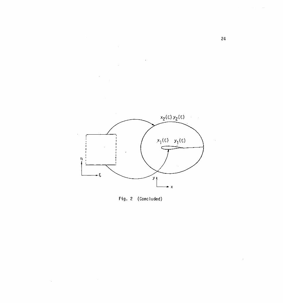
I
I I I
1=, (Concluded) Fig. 2
24
25
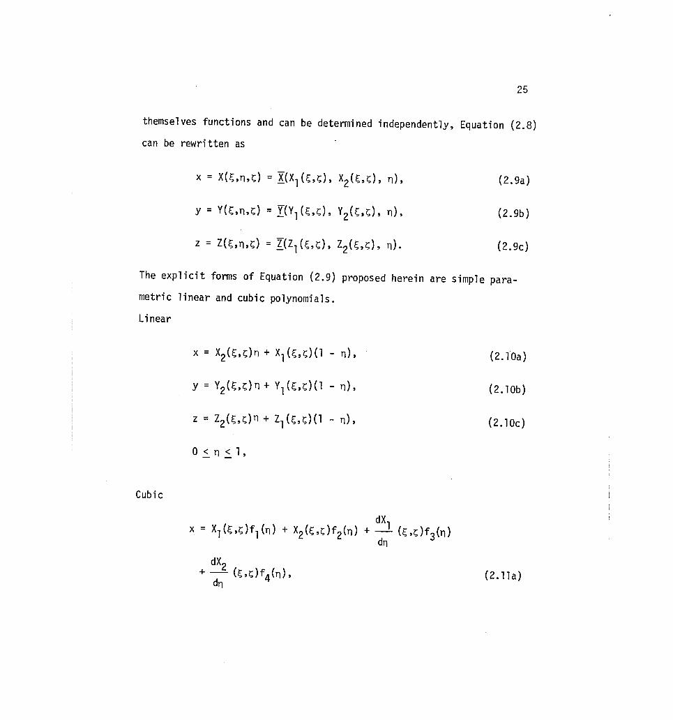
themselves functions and can be determined independently, Equation (2.8)
can be rewritten as
(2.9a)
(2.9b)
(2.9c)
The explicit forms of Equation (2.9) proposed herein are simple para
metric linear and cubic polynomials.
Linear
(2.1Da)
(2.1 Db)
(2. 1 Dc)
Cubic
(2.11a)

26
(2.11b)
(2.11c)
where:
f1 (n) _ 3 2 - 2n - 3n + 1 ,
f2(n) 3 2 = -2n + 3n ,
f3(n) 3 2 = n - 2n + n,
f4(n) 3 2 = n - n ,
A function such as Equation (2.10) or Equation (2.11) is topologically
referred to as a homotopy [24J. Blending-function [llJ is another
name that has been given to such equations for problems in surface
design. Herein, because of the context in which they are used, they
are defined as IIconnecting functions. 1I

27
Applying a cubic connecting function implies that the physical
grid can be forced to be orthogonal" at the boundaries since the deriva-dX dX
tives ~(s,~), ~s,~), etc. can be computed from the cross product n n dXl dXl dYl dY l of the tangential derivatives ~(s,~), ~(s,~), ~(s,~), ~(s,~),
etc. That is,
dX dY --.! (s,Z;) i + --.! (s,~) r dZ R, .,r
+ - (s,~)1< = dn dn dn
+ + j( 1 J
dX dY dZ K ~ (s,~) ~ (s,~) ~ (s,~) R, = 1,2
ds ds ds
dX ~ (s,Z;)
dY --.! (s,d
dZ 2 (s,d
d~ d~ d~
+ + + where i , j, and k are unit vectors and K is the magnitude of the
normal vector. Applying this procedure will force the grid to be
orthogonal at the boundaries but not necessarily anywhere else. For the
linear connecting function, the physical grid will seldom be orthogonal.
Given the connecting function and parametric boundary functions,
a uniform computational grid can be mapped onto the physical domain
forming a physical grid. Concentration of grid points in the n direc
tion is accomplished by choosing a function n = n(n) such that

28
O~n~l, - dTi ( ) o ~ n ~ 1, and dn > 0 Fig. 3 . For example, contracting
the physical grid towards one boundary or the other can be accomplished
by
1\
ekn _ 1
n= ~ ; O~n~l. e - 1
(2.12)
"-
where k is a free parameter whose magnitude dictates the degree of
contraction. Embedding this exponential function in the linear con
necting function, Equation (2.10) becomes:
x = X2{~,~)n + Xl{~,~){l - nL
y = Y2{~,~)n + Yl{~,~){l - Ti)'
z = Z2{~,~)n + Zl{~,~){l n) ,
o < n < 1.
Once the connecting function has been chosen, the remaining prob
lem is the determination of the boundary functions which are independ-
ent of n. For the "two-boundary technique" the approach is to choose
parametric variables sand t associated with the boundaries such
that
xl (~,l;) + Xl (s,t),

1
-11
o
n = ri(l1)
dn > 0 dl1
11
Fig. 3 Grid control function.
29

s. <5<5, mln - - max
t. <t<t . mln - - max
30
The choice of parametric variables can vary from problem to problem.
A relationship between (~,~) and (s,t) is
This is a linear relation which maps the unit interval onto the
parametric variables. Control of the physical grid at the boundaries
is accomplished in the same manner as for the connecting function.
That is,
d~ > 0 d~ ,
~ = ~(r;), ~~ > 0,
Since the connecting function is dependent on the boundary position,
control of the entire grid is accomplished.
2.4.1 Approximate Boundary-Fitted Coordinate Systems
Using Tension Spline Functions
31
It is often the case that boundaries in a physical domain are
described by discrete sets of points. The boundaries may be open or
closed (Fig. 2). An approximate boundary-fitted coordinate system can
be obtained using the IItwo-boundary technique ll and a tension spline
function interpolation to the discrete data defining the boundaries.
Tension splines [17-19] are chosen because standard cubic splines [25]
and other higher ordered interpolation techniques often result in
wiggles in the approximation. Wiggles on a boundary using the IItwo
boundary technique ll propagate into the interior grid. The tension
parameter embedded in the tension spiine interpolation allows control
of the IIcurvednessll of the approximation. A very large magnitude of
the tension parameter corresponds to a linear interpolation whereas a
very small value corresponds to cubic splines. Tension splines can
be applied in two and three dimensions. A two-dimensional example is
presented.
Using the tension spline technique, a point set on boundary one i-n j=m
is defined by {xi 'Yi}i=l and on boundary two by {xj'Yj}j=l.

32
Approximate arc length is used as a parametric independent variable. The
approximate arc length is:
s· = [(x i+1 1
s. = [(Xj +1 J
i = l ... n
j = 1. .. m
s - 0 1 -
o < s. < s - 1 - n
o < s. < s . - J - m
x.)2 + 1/2
(Yi+l _ y. )2] + s. l' 1 1 1"
2 1/2 - Xj ) + (Yj+1 _ y.)2] + s. l' J J-
From the computational coordinate system the unit interval (0 ~ ~ ~ 1)
must be mapped onto each boundary; that is:
s = s(~),
This is accomplished by letting
s = ~sn on boundary one and
s = ~sm on boundary two.

33
The tension spline function is a piecewise continuous set of trans
cendental functions where x and y between the ~ and ~ + 1 points
are defi ned by
II sinh[a( s~+l - s)]
x = 9 (s ~) -:2~'~---';'':''-;''---a sinh[a(s~+l - s~)]
(2.13)
sinh[a(sn+l - s)] y = h" (s ) --;:;-__ ..::.N:.:...!. ___ _
~ a2sinh[ (s~+l - s~)]

s = s(~) = ~,smax'
~ = i on boundary one,
£ = j on boundary two,
a = tension parameter.
The unknowns in these equations are
are second derivatives at the data points
gll(S£) and hll(S£) £=N
{x£'Y£}£=l where
34
(2.14)
which
N = n for
boundary one, N = m for boundary two, and are obtained through enforce
ment of the continuity of the first derivatives at the data points and
the specification of two end conditions. A tridiagonal system of
linear equations results for each set of unknowns. The solution of the
tridiagonal systems yield gll(S£) and h"{s£).
The cubic connecting function (Eq. 2.11), and the exponential
function (Eq. 2.12) provide the relationship between the computational dX£ dY£
domain and the physical domain. The derivatives dn and an- are:
ds
dY.e dX.e = -K-.
dn ds
By defining a grid with constants ~~ and ~n in the computational
domain a corresponding grid is explicitly defined in the physical
domain.
35
An example of a grid about a Karman-Trefftz airfoil is presented
using the spline under tension approximation to the boundaries and a
cubic connecting function. Table 1 contains the data describing the
airfoil boundary and outer boundary. Figure 4 shows the approximation
to the airfoil boundary and Figure 5 shows the grid. A tension parame-
ter value of 2 is used. Transformation data have not been computed
for this example.
2.4.2 Transformation for a Wedge-Cylinder Corner
An application of the two-boundary technique using analytical sur
face functions is a family of three-dimensional corner geometries which
occur in many aerodynamic situations (Fig. 6). Supersonic flow about
these geometries is characterized by strong visid-inviscid interactions
which are adequately analyzed only through the numerical solution of
the Navier-Stokes equations. When solving this system of equations
with a finite difference technique, a grid must be designed to capture
the interactions and allow for accurate application of the boundary
conditions.

Table 1. Data description for an airfoil grid
Ins i de boundary Outside boundary
x ft. y ft. x ft.
. 49950 -.000031 0.0
.49860 -.001400 2.12
.49600 -.002760 3.0
.48620 -.005550 -2.12
.47060 -.008510 0.0
.39010 -.028590 -2.12
.26960 -.029970 -3.0
.12270 -.040790 -2.12 -.03480 -.048450 0.0 -.18750 -.050520 -.32110 -.045590 -.42390 -.0377390 -.48650 -.016530 -.50270 .003820
I I
-.47110 .026640 I -.39690 .048640 I
-.28790 .066100 -.15380 .075290 -.00560 .074530
.14400 .064350
.28230 .04750
.39580 .028260
.47200 .011300
.48710 .006810
.49510 .003040
.49880 .001430
.49950 -.000031
Y ft .
3.0 2.12
. 0.0 -2.12 -3.0 -2.12 0.0 2.12 3.0
I
'...v Q)

37
cC:_eo_O_-Eo:r-°_-e:'-~_-I:r-
Fig. 4 Boundary definition for Karman-Trefftz airfoil.

Fi g. 5 Gri d for Karman-Trefftz ai rfoil obtai ned with the IItwo-boundary techni quell .
w co

39
y
~z
Rectangul ar corner Wedge-plate corner
Plate-cylinder corner Wedge-cylinder corner
Fig. 6 Three-dimensional corner geometries.

40
The "two-boundary technique" is app 1 i ed to the wedge-cyl i nder cor
ner with the aid of Figure 7. The other corner geometries are derived
from the wedge-cylinder definition. The physical domain is the region
enclosed by the circular cylinder with radius rO' an outer surface
defined by the wedge angle and a second cylinder radius, and two planes.
The left plane (wedge surface) is oriented at an angle cp (wedge angle)
with the longitudinal axis of the cylinder but parallel to the vertical
axis. The right plane (symmetry plane) is oriented with angle 82
relative to the vertical axis of the cylinder and includes the longi
tudinal axis. The upstream and downstream boundaries are cross sections
of the region defined by x = Xo and x = xL and are perpendicular to
the longitudinal axis. The "two-boundary technique ll is applied to this
geometry by considering the inside cylinder surface as boundary one and
the outside surface as .boundary two. It is desired that ~, n, and ~
map into the region described above and that
The boundaries are defined by

y
~------------------------------------------------ z
x -----------t ... _ ~
-==============£f =S<pC==JI h
Fig. 7 Projection of wedge onto the x-y plane and cross section of grid in the y-z plane.
41

42
Boundary one:
(2.15a)
(2.15b)
(2.15c)
Boundary two:
(2. 16a)
(2. 16b)
(2.16c)
Where:
e = sin-1 (X(~) tan p) 1 r' a
e = sin-1 (X(~) tan p) 3 r' 1

43
A linear connecting function is used to generate the internal grid.
The function is
z = Z2{~,~)n + Zl(~,~)(l - n),
k2n e - 1
n = ---;----k2
e - 1
(2.l7a)
(2.l7b)
(2.l7c)
(2.l7d)
An exponential function is used on both n and ~ to concentrate the
grid in the corner. Figure 8 shows the grid at x = xL for cor
responding corner surfaces shown in Figure 6. The planar corners are
closely approximated by letting the radii be very large.

I
'I
I
• ~ ~
Rectangular corner 60 wedge-plate corner 12.20 wedge-plate corner
Plate-cylinder corner 60 wedge-cylinder corner 12.20 wedge-cylinder corner
Fig. 8 Grids for wedge-plate and wedge-cylinder corners at x/xL = 1. of::> of::>

45
Information needed for the equations of motion (Eq. (2.3)) is the
transformation data which is obtained from Equation (2.7). The deriva
tives in Equation (2.7) are obtained by analytic differentiation of x,
y, and z (Eq. (2.17)) with respect to ~, n, and s. These deriva-
ti ves are:
ax _ an - °
~ = n ~~ (s,l,s) + (1 - n) ~ (~,O,s)
El.= anY(s,l,s) - ~~ Y(s,o,s) an an
El.--£.l( ) ( ::l£.l( ) as - n as s,l,s + 1 - nJ as s,o,s
az - az ( ) ( -) az ) a[ = n ~ s,l,s + 1 - n ~ (s,O,s
az _ an ( ) an an - an Z s,l,s - an z(s,l,s)
az - az ( ) ( -) az ( ) az = n az s,l,s + 1 - n az s,o,s

\'Ihere
a8 n- (c;,Q,r;;) = -r1
sin[~82 + (1 - ~)81J(1 - rJ _1 a~
az a8 1 at (~,O,r;;) = r 1 cos[~e2 + (1 - ~)81 J[l - U -a~
-az - - J k ~ (~,o,r;;) = r 1 cos[~e2 + (1 - r;;)8 1J[8 2 - 81 ar;;
-
~~ (~, 1 ,r;;) = r 2 sin[~e2 + (1 - ~)83J[82 - 83J ~
46
1
_dr_2 _ l x tan ¢ ~ r 2 d~
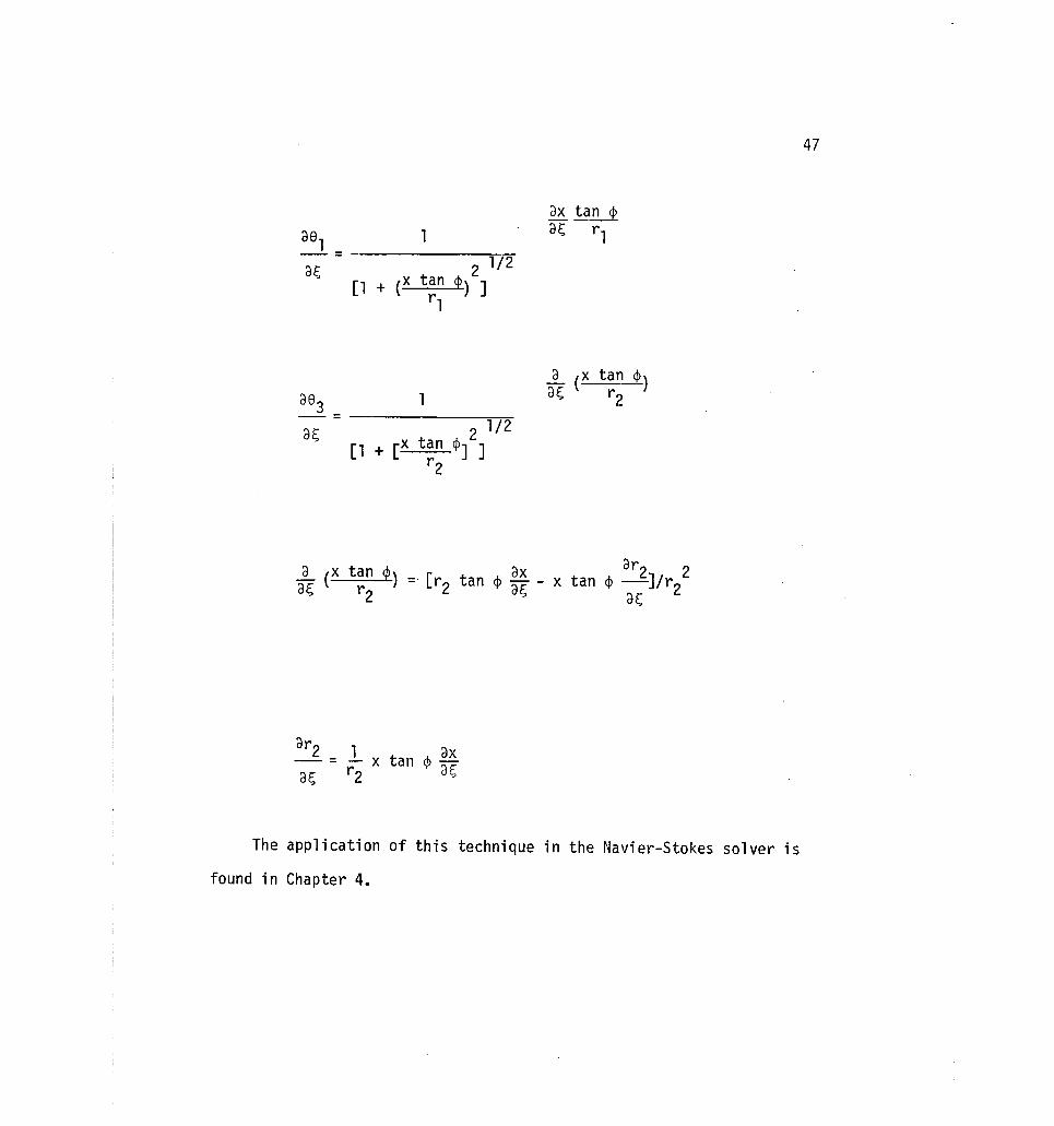
The application of this technique in the Navier-Stokes solver is
found in Chapter 4.
47

48
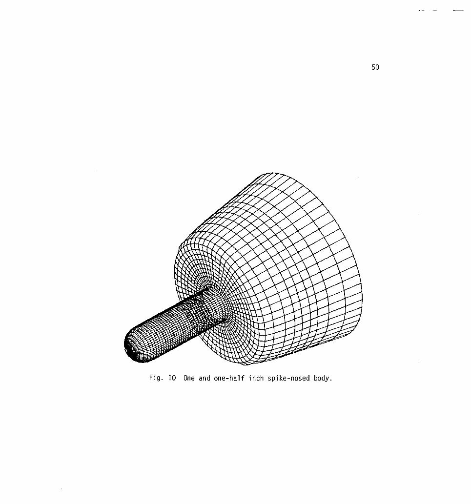
2.4.3 Transformation for a Spike-Nosed Body
The "two-boundary technique" is applied to generate grids about
spike-nosed bodies (Fig. 9 and Fig. 10). Supersonic flow about these
bodies is unsteady and separation occurs in the nose-shoulder region.
Consequently, grids must be concentrated in the nose-shoulder region
and be ~dequately spaced to define the shock and the boundary layer on
top of the shoulder. A linear approximation to the inner boundary and
a circular arc outer boundary are used in the two-boundary technique.
Concentration of the grid is accomplished by superimposing an exponen
tial function onto the connecting function and a combined exponential
and parabolic algebraic function is superimposed onto the parametric
variable along the boundaries. The grid is cast in three-dimensions by
rotating the two-dimensional description about the axis of symmetry.
The inside boundary ;s defined by the set of points
The parametric variable associated with this boundary is accumulated
cord length where
'" tl = 0, and

49
Fig. 9 One-half inch spike-nosed body.
50
Fig. 10 One and one-half inch spike-nosed body.

51
\~ith the parametric variable defined, two data sets are formed. They
are:
A linear approximation to the inside boundary for a spike-nosed body is
accomplished by linear interpolation of the above data sets. The trans
formation data requires the derivatives of the boundary definition with
respect to the parametric variable and the derivative sets are formed
and saved for later use. The derivative sets are:
( dx I M-l
dyI o.=M-l
la' A
t , dto.
a dto.
0.=1 0.=1
where
"I A A "I "I dx xa+l - x a-l dyI = Y a+ 1 - Ya-1 =
A
- t dt " " dt ta+l a-1 ta+1 - t a-l a a
a = 2 . . . . M-l.
The linear interpolation to the point sets can be symbolically written

-= dt
dt (
"I A dy
Li ndy" t'-A a dt
where Lin denotes a linear interpolation.
a=M-1)< .
a=2
The outside (top) boundary is a circular arc defined by
xO = -R cos 0 + ~ o
"0 y = " R sin 8 + Yo.
The physical domain in two dimensions is the region between the
52
inside and outside boundaries. A rectangular region can be mapped onto
the physical domain based on information from the boundaries and a
linear connecting function. The transformation is
""0 I Y = Y n + y (1 - n).

j=m . }k=m Given the computational grid {sJok' nOk
J j=l
where
j=n r. j=m y ok}
J j=l k=l
k=l
the physical grid is
Concentration of the grid near the inside boundary and in the nose-
shoulder region is accomplished by intermediate transformations
ern - 1 n = ---- ,
e k - 1
and
53

54
The parameters ~, ~l' and B govern the concentration of the grid
pcints. The above derivation for the transformation between a computa
tion domain and a physical domain is for a two-dimensional slice of a
flow field. A three-dimensional representation is
(2.l8a)
(2. l8b)
(2.l8c)
The elements of the Jacobian matrix are:
ax = at

A
~ = [COS(~[~max - ¢min] + ¢min)] ~ ,
az a( = 0,
"'-az ax = an an'
az a I;; =
"'-
ax ~'
55

'" "'0 ax - ax = n 3Z dO ae as + (1 _ ~) as az;;
'" a-n dV _ "'0 an "'I frl - Y an - Y an '
~ = - ayo ae a~ + (1 _ n) a? at a~ as n ae as ~ at as ~,
kn an
_ e = k an
eK -
a~ _ ~1 __ ~ - k1
e - 1
axO
1
ae = R sin e,
ayO = ae R cos 8,
(1 + 8s - 8s2)k1 (ekg - 1)(8 - 2Bd
(1 + Bs - Bs2)2
56

--
Fig. 11 Grid generated with the "two-boundary technique" for a one-half inch spike-nosed body.
57

---
Fig. 12 Grid generated with the "two-boundary technique" for a one and one-half inch spike-nosed body.
58

Table 3. Data description for a one and one-half inch spike-nosed body Inside boundary
Pt x y Pt x y Pt x
1 0.0 0.0 21 .01042 .01804 41 .12475 2 .00003 .00109 22 .01138 .01856 42 .12494 . , 3 .00011 .00218 23 .01236 .01903 43 .12500 4 .00026 .00326 24 .01337 .01945 44 .12500 5 .00046 .00433 25 .01440 .01981 45 .12500 6 .00071 .00539 26 .01544 .02012 46 · 12500 7 .00102 .00644 27 .01650 .02038 47 .12506 8 .00138 .00747 , 28 .01757 .02058 48 .12525 9 .00180 .00847 29 .01866 .02072 49 .12556
10 .00227 .00946 30 .01974 .02080 50 .12597 11 .00279 .01042 31 .02083 .02083 51 · 12649 12 .00336 .01135 32 .02163 .02083 52 · 12708 13 .00398 .01225 33 · 12000 .02083 53 · 12774 14 .00464 .01311 34 · 12083 .02083 54 · 12844 15 .00535 .01394 35 · 12156 .02090 55 .12873 16 .00610 .01473 36 .12226 .02108 56 · 12883 17 .00689 .01548 37 .12292 .02139 57 .25000 18 .00772 .01619 38 .12351 .02181 OutSide Boundary
19 .00859 .01685 39 . 12403 . 02232 ~o = .43333 ft . R = .52208 ft •
~2 = .0001 YO = ·.07500 ft .
20 . 00949 .01747 40 · 12444 .02292 kl = 2.2 B = 2
y
.02357
.02428
.02500
.02667
.07417
.07533
.07606
.07676
.07742
.07801
.07853
.07894
.07925
.07944
.07948
.07949
.09929
8f = 69.5°
80 = 8.295°
I
0) o

Pt
1
2
3
4
5
6
7
8
9
10
11
12
13
14
15
16
17
18
19
20
Table 2. Data description for a one-half inch spike-nosed body
Inside Boundary
x y Pt x y Pt x y
0.0 0.0 21 .01042 .01804 41 .04142 .02397 .00003 .00109 22 .01138 .01856 42 .04161 .02428 .00011 .00218 23 .02136 .01903 43 .04167 .02500 .00026 .00326 24 .01337 .01945 44 .04167 .02667 .00046 .00433 25 .01440 .07981 45 .04167 .07417 .00071 .00539 26 .01544 .02012 46 .04167 .07533 .00102 .00644 27 .01650 .02038 47 .04173 .07606 .00138 .00747 28 .01757 .02058 48 .04192 .07676 .00180 .00847 29 .01866 .02072 49 .04223 .07742 .00227 .00946 30 .01974 .02080 50 .04264 .07801 .00279 .01042 31 .02083 .02083 51 .04316 .07853 .00336 .01135 32 .02163 .02083 52 .04375 .07894 .00398 .01225 33 .03666 .02083 53 .04441 .07925 .00464 .01311 34 .03749 .02083 54 .04511 .07944 .00535 .01394 35 .03822 .02090 55 .04550 .07948 .00610 .01473 36 .03892 .02108 56 .04549 .07949 .00689 .01548 37 .03958 .02139 57 .16687 .09929 .00772 .01619 38 .04018 .02181
Outside Boundary .00859 .01685 39 .04070 .02232 Xo = .4333 It. Radius = .52208 It. 01 = 51.550
.00949 .01147 40 .04111 .02292 ~2 = .0001 Yo = .07500 It. Or) = 8.2950 kl = 2.2 B ~ L t.-'
I.D

61
A I (I A I t1= 1 ) ax . A dx
-,,- = L lndx t a , (j7f at a a=2
" at --
Grids generated with this application of the IItwo-boundary technique"
to the bodies shown in Figures 9 and 10 are shown in Figures 11 and 12.
Tables 2 and 3 give the data used to generate the grids. The use of
the grid in the Navier-Stokes solver is discussed in Chapter 4.
2.5 Initial and Boundary Conditions
Initial conditions are free stream conditions except at solid
boundaries where no slip is imposed on the velocity. Free stream con-
ditions are established from the Mach number = Moo, Reynolds num-
ber = Re = Re, characteristic length = L, and free stream tempera-00
ture = T. The speed of sound is 00
62
where y = 1.4 and Cv = 4290 (~)2 ---dl for air which is considered sec· eg a perfect gas. The free stream velocity is
v = 0 , 00
and
w = 0 . 00
The free stream viscosity is
lloo =
-8 3/2 2.27 x 10 Too
Too + 198.6
The free stream density, pressure, and energy are
and

63
No slip boundary conditions are imposed on the velocity at solid
walls. A solid wall is considered to be isothermal and the tempera
ture TW is fixed. The boundary condition on energy is eW = CVTW
The solid wall boundary condition for density = pW is obtained
through a condition on pressure at the wall and the relation of density
to pressure in the equation of state. The wall pressure boundary con
dition is obtained by approximately satisfying the momentum equations
at the wall. Assuming that the gradient of the shear stress is zero
at a solid wall implies that ;~ = 0 where N indicates the normal
direction.
In general, the zero pressure gradient boundary condition at a
solid surface can be enforced given the direction cosines (Yx' yy' yz)
of the normal vector on the surface. Then
an "\ ap\ ax ax aE;
api aE; an
~) ap
= o. (2.19) = (\YyYz) ay ay ay an aN w
an a I:; ap az az ~

2.5.1 Boundary Conditions for Supersonic Flow About
Wedge-Cylinder Corners
64
For wedge-cylinder geometries the transformation between the com
putational domain and the physical domain is given by Equation (2.17).
The upstream boundary conditions at ~ = 0 are the free stream condi
tions. Solid walls occur at n = 0 and s = 0 for ~ > O. For n = 0
the condition ~ = 0 + ~ = 0 where r is the radial direction from aN ar the center line of the cylinder.
~I = ar n=O
ap .£l. + ap az + ay ar az ar
ap ax ax ar = O.
From Equation (2.17)
~ A
= COS(s82 + (1 - ~81) = cos 8 ar
az sin(s82 + (l - ~)el) A
= = sin e ar
ax O. = ar
Therefore,
api ap 9 + ~~ sin A
= ay cos e ar n=O
and
api (~ ~ + ap an + ~~) cos A
= e or n=O o~ oy on oy os oy
(~~+ ~ on + ~~) A
+ sin e o~ az on oZ Os oZ

65
where
_ elements of the Jacobian matrix at n = O.
• at,; at,; Slnce ay = az = 0,
ap an is approximated by the one-sided difference
and, ~~ approximated by the central difference
Then
where
ap P2,k+l - P2,k-l az=
api (3Pl ,k - 4P2,k + P3,k) P2 k 1 - P2 k 1 - = C + ( , + , - ) C2
= 0, ar n=O 2~n 1 2M;
Cl = an cos ay e + an sin A
az e
a I;; A dl;; A
C2 = - cos e + az sin e. ay

66
Consequently, the pressure on the boundary n = 0 is approximated by
_ lln C2 -C (P2k1-P2,k-1L
3llt;; 1 ' +
The normal pressure gradient boundary condition a~1 = 0 for aN 1';=0
the wedge surface of a wedge cylinder corner is
aNP = ap (-sin cp ~) + EE. (an (-sin cp) + aanz cos cp) a a~ ax an ax
+ ~ (~(-sin cp) + ~ cos cp) = 0 at;; ax . az
where the directional cosines are: Yx = sin cp, Yy = 0, Yz = cos cp.
The finite difference approximation for P at I'; = 0 is
P .. 1 = 1 ,J ,
4P .. 2 - P .. 3 l,J, l,J,
3
f1r;, D2 - (P .. 1 2 - P .. 1 2)
3lln D l,J+, l,J- , 1
D3 - (P .. 2 - P. 1 . 2) D l,J, 1- ,J,
1 where,
and
D1 = ~~ (-sin cp) + ~i cos cp,
D2 = ~~ (-sin cp) + ~i cos cp,
D = 3 . a~ -Sln cp -ax .

67
The far field boundary conditions (~= 1, n = 1, ,= 1) are
~I = 0 ~I = 0, and a~ ~=l 'an n=l
aUI = O. The condition ~~ = 0 al;; 1;;=1 ."
implies that there is no change in the state variables with a change
in ~. The approximation is Ui = Ui _l . The condition ~~ = 0 implies
that there is no change in the state variables with a change in y. For
the wedge-cylinder corners, this implies two-dimensional flow on a flat
plate and/or inclined plate. That is:
au = au a~ + ay a~ ay
au a I;; = ~ ay o.
Noting ~ = 0 and applying the finite difference approximation ay
imp 1 i es
a I;;
"* (U j -1 ,k+ 1 - U j -1 ,k -1 ) • ay
au The condition ~ = 0 implies that there is no change in the state
variables at I;; = 1 or that symmetry is imposed. In either case
I;;k = I;;k_1 for this study.

68
2.5.2 Boundary Conditions for Supersonic Flow
About Spike-Nosed Bodies
The transformation between a computational domain and the physical
domain for spike-nosed bodies is given by Equation (2.18). In this
case the solid surface is at n = 0, 0 ~ ~ ~ 1, and 0 S ~ < 1. No
slip conditions are imposed on the velocity and the temperature is
fixed. The pressure is found in a similar manner to that used for the
wedge-cylinder geometries except a less accurate approximation to the
zero pressure gradient is used. In this case a first order approxima-
tion is used and the pressure on the solid boundary is set equal to the
pressure at the grid point next to the boundary. That is:
Pi,l,k = P. 2 k' 1, ,
The density at the boundary is found by the application of the equation
of state using the boundary temperature and computed pressure.
At s = 0, 0 ~ n ~ 1, and 0 ~ ~ ~ 1 a symmetry boundary condi
tion i.s imposed. The three-dimensional grid is obtained by rotating
a two-dimensional slice of the grid about the axis of symmetry. The
1 i ne ~ = 0, o ~ n < 1, and 0 < ~ < 1. is coincident with the line of - -symmetry. The Jacobian matrix (Eq. (2.7)) is singular along this line.
This does not create a problem, however, since the condition is imposed
without using the transformation data from this line. The symmetry
condition is

69
aUI a~ ~=o = 0 or U;,j,l = ~i,j,2'
Free stream boundary conditions are imposed at n = 1, 0 ~ ~ ~ 1,
and 0 < ~ ~ 1. At ~ = 1, 0 ~ n ~ 1, and 0 < ~ ~ 1 a no-change
boundary condition is imposed. That is:
aUI = 0 a~ ~=l
or U. . N = U. . N l' 1 ,J , 1 ,J, -
3. COMPUTATIONAL ASPECTS
The computational requirements for computing a grid and the
Jacobian matrix associated with a grid using the "two-boundary tech
nique" are relatively minimal. It is however, necessary to plot the
grid to visually assure that the desired constraints are satisfied.
Ultimately, this phase of problem solving should be in an interactive
mode with high bandwidth communications between the computer and a
graphics terminal. The transformation data for an acceptable grid can
be stored on a permanent file for later use. An alternate approach is
to program the equations for the Jacobian matrix within a program for
the solution of a flow-field. In this manner only parameters for
the grid generation must be supplied.
The computational requirements for the solution of the three
dimensional Navier-Stokes equations are extreme and tax the capability
of any presently existing computer [1]. The approach taken in this

70
study is to adapt a viable numerical technique to the available large
scale computer. The computer is the STAR-100 or its successor the
CYBER 203. The computer architecture is based on vector processing
with virtual memory storage. In addition to the vector architecture
there are two aspects relative to the computer that have been very
important in this study: (1) the capability of halfword arithmetic
and storage; and (2) the effect of data transfer between secondary
memory and primary memory. Halfword arithmetic has been used almost
exclusively in the computations discussed later allowing for much
larger grids than would be otherwise possible. Frequent transfers of
data from primary memory to secondary memory and back have been
minimized or avoided by' constraining the grid size on which a solution
is attempted. The transfer of data to and from secondary memory is
relatively inefficient and is discouraged by high cost to the user.
Another computational aspect is that the "Navier-Stokes solver"
is relatively general. The application of initial and boundary condi
tions are performed in separate subroutines from the general solution
procedure. Defining a new problem by initial and boundary condition
does not require major programing modifications.
In this chapter the MacCormack time-split algorithm is examined
and vectorized for the CYBER 203 computer. Also, the program organiza
tion and how it relates to the virtual memory is presented.

71
3.1 Computational Technique
The computational technique used in this investigation is the
MacCormack time-split predictor-corrector algorithm [2-4J which was
proposed about 1970 and is a derivative of the MacCormack unsplit pre
dictor corrector algorithm [26J. Both techniques are explicit which
implies that they are time step stability limited [27J. Also, both
techniques are second order accurate, and many investigators have been
highly successful in applying them to a variety of fluid flow simula
tions [1,3,4,28J. An advantage of the MacCormack techniques is that
they are relatively easy to apply to the transformed equations of
motion (Eq. (2.3)). The split operator algorithm has the added
advantage that different time step magnitudes can be used in each
operator. A third hybrid scheme [29J can be applied by subdividing
the operators into implicit and explicit portions. This approach, how
ever, is more complex and the success of its use is somewhat case
dependent [30-31J. The explicit time-split technique has been chosen
for this investigation because of its simplicity and vectorization
characteristics for application on the CYBER 203 computer, however,
both the unsplit and split algorithms are presented herein for contrast
and clarity.
3.1.1 MacCormack Technique
The unsplit algorithm has the following two steps applied to the
transformed equations of motion (Eq. (2.3)).

72
Predictor step:
;-;flu +' Un .. k = l·,J·,k 1 ,J ,
(F. - F. ,) ~i; i + (G. - G. ,) ~~ i + (H. - H. ,) ~~ i 1 1- oX 1 1- oy 1 1- oZ
j,k
i,k
i ,j

Corrector step:
un+1 i,j,k = 1
2" (u~. + U~+~ 1,J,k 1,J,k
~t [{F F } a~. (G _ G.) ~ i + (H. +1 - H.) ~s i J - ~~ i + 1 - i ax 1 + i + 1 1 ay 1 1 Z j,k
- ~~ [(Fj +1 - Fj ) ~~ j + (Gj +1 - Gj ) ~~ j + (Hj +1 - Hj ) ~~ j J. l,k
73
- ~~ [(Fk+1 - Fk) ~~ k + (Gk+1 - Gk) ~~ k + (Hk+1 - Hk) ~i kJ . . )' •
1 ,J

74
This algorithm is applied for a time step by passing through a
data base consisting of the state v'ariab1es (p, pu, pv, pw, pe) and
the transformation data and applying the predictor step. The corrector
step is applied with the output of the predictor step, and the old
state variables in the data base are replaced with the new values.
The algorithm is repeated until a steady state solution is reached or
an otherwise chosen stopping point is reached.
3.1.2 MacCormack Time-Split Technique
The split algorithm consists of a predictor and corrector step
for each coordinate direction. Consequently, a predictor and corrector
step for a coordinate direction is called an operator for that direc-
t ion (i. e. , Ld
• t. (time step)). A time step is completed in 1 rec lon
this algorithm with the application of each operator applied sym-
metrically about the operator for the coordinate direction of primary
flow. That is, for the corner flows studied herein
un+1 i ,j ,k =
n u .. k 1 ,J ,
where

75
For the spike-nosed body flow
where
Each operator is defined by an output state solution Uout for a
given input state solution Uin • Therefore,
where
Predictor step:
in t- tt;. ~ ) t-t;." (G G ) at;. " o - U 1" , J" ,k - -V F i - F i - 1 ax 1 + i - i - 1 ay 1 i,j,k - <,

76
Corrector step:
uout = 1 luin + IT - !1Atf [(F'.+l - F.) a(. i i,j,k 2 ,i,j,k i,j,k us , ax
L (!1t ) = Uout n n i ,j , k
\'/here
Predictor step:
+ (H j - H j -1) ~i jJ i , k

77
Corrector s~:
Uout = 1 u in + IT _ --1l (F F ) an . (
lit [ i,j,k 2 i,j,k i,j,k lin j+l - j ax- J
Lr(lIt r } = uout ~ ~ i,j,k
where
Predictor step:

78
Corrector step:
uout = 1 (u in + IT - ~~ [(Fk+l - Fk) ~xz; k i,j,k 2 i,j,k i,j,k u~ a
The unsplit algorithm requires only one pass through the data base per
time step while the split algorithm requires several passes through the
data base per time step. When the data base exceeds the primary stor
age capacity of the CYBER 203 computer a time penalty is imposed when
data is called from secondary memory. However, a data management pro-
cedure has been implemented to minimize the penalties associated with
the use of secondary memory.
It has been noted that the MacCormack algorithms are second order
accurate. Forward and backward differences are applied such that after
the predictor and corrector steps are completed an effective central
difference approximation is obtained [3J. This is demonstrated with
derivatives of velocity components required in the viscous stress
terms. Consider
au au au a~' an and ~
79
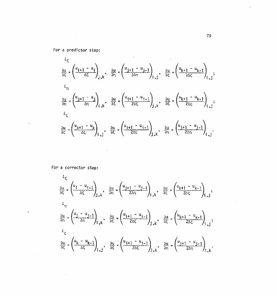
For a predictor step:
Uj _1) , .£!! =(Uk+1 - Uk- 1) ; .. a~ . a6~ . . 1 ,J 1 ,J
Ln
au _ (Uj +1 - Uj ) an - 6n i ,k'
L~
~~ . (Uk+!,- Uk)i,j' ~~. (Ui+~fi~ Ui-1)j,k'
For a corrector step:
~ = (Uk+ 1 - Uk- 1) . a~ 26~ . .'
1 ,J
~ = (Uk+1 - Uk- 1) . a~ 26~ " '
1 ,J

80
The unsplit and split MacCormack algorithms are time step stabil
ity limited, and there is no complete stability analysis to indicate
the maximum allowable time step. A conservative time step employed by
Shang and Hankey [3-4] has been used. This time step is
tJ.t < min [JQl + ~ + ~ + C - tJ.x tJ.y tJ.z
where
c - local speed of sound,
_1_ + _1_ + _1_ tJ.i tJ.y2 tJ.z2 ]
-1
A point that must be considered in the application of the
MacCormack algorithms to viscous compressible flow with strong shock
waves is the inclusion of terms to dampen oscillations in the region of
a shock. A pressure dampening term suggested by MacCormack [31] is
included in the finite difference approximation to the equations of
motion. This term is
-CintJ.tno~ ~~ JV JV JV OUR,
where
au a0R,
R, = 1,2,3

81
3.2 Application of Vector Processing to the Computational Technique
The MacCormack time-split algorithm has been programmed to run on
the CDC STAR-lOa and CYBER 203 computers. The program called the
fJavier-Stokes solver was first written in STAR FORTRAN and is described
by Smith and Pitts [32]. The program has since been written in the
SL/l language [20] where 32-bit arithmetic is used to increase the com
putational speed and incore storage.
3.2.1 Vector Processing Using the CYBER 203 Computer
The CYBER 203 is a vector processing computer capable of achieving
high result rates when a high degree of parallelism is present in the
computation. When an identical operation is to be performed on consecu
tive elements in memory, a vector instruction is issued to perform the
operation. Each vector instruction involves a time penalty, called
vector startup, regardless of the length of the vector. As the length
of the vector increases, the operation becomes more efficient since the
penalty becomes relatively less important.
The CYBER 203 has about one million words of primary memory with
virtual memory architecture. Memory is referred to as pages. The two
page sizes on the CYBER 203 are IIsmallll pages which are 512 64-bit words
and 1I1arge il pages which are 65536 words or 128 small pages. A user can
have access to about 15 large pages in primary memory at anyone time.
The movement of data from secondary memory into primary memory involves
moving pages of data in and out of primary memory. This is called a
IIpage fault ll and involves a startup time and transmission time just as
82
vector operations do. It then becomes important to make the most
efficient use of the data when it is in primary memory in order to
avoid a situation where the machine is spending more time moving pages
of data in and out of primary memory than it is spending on actual
computations. This is often referred to as IIthrashing." Storing the
data for a large data base program, such as a three-dimensional
Navier-Stokes solver, in a conventional manner could very possibly
lead to this situation. If, however, you design an interleaved
data base [33] where the variables that are currently being used are
stored together then it could result in less movement of "pages ll of
data.
A capability of the CYBER 203 architecture is half-word arith
metic. This means that computation can be performed with 32-bit
words and approximately two million 32-bit words can be stored in pri
mary memory. The speed of computation is approximately twice that
achieved with 64-bit operations. A high level programming language
SL/l [20] is used to access the half-word capability. It is shown in
the next chapter that for the MacCormack time-split algorithm 32-bit
arithmetic is quite adequate and the computational speed and primary
storage are approximately doubled as compared to FORTRAN version which
uses 64-bit words.
3.2.2 Program Organization and Data Management
The Navier-Stokes solver is a derivative of a serial FORTRAN
code which operates on the CDC-CYBER 175 and 7600 computers [2-3].

83
Seven of the nine elements of the Jacobian matrix are programmed into
the serial code and some redundant computation is performed to coexist
with available memory. The Navier-Stokes solver is written in SL/l and
maintains the MAIN program logic and time step calculations found in
the serial code (Fig. 13). The operator calculations are redesigned
around the vector architecture of the CYBER 203 computer. Also, all
nine elements of the Jacobian matrix are included in the new code.
Normally it may be thought that vector lengths should be equal to
the total number of grid points and vector operations sweep through the
entire grid with each variable dimensioned to the number of grid points.
However, for the number of variables involved and the large number of
grid points this leads very quickly to the IIthrashingli situation
described earlier •. Instead, vectors are computed in planes in the
~ directions (Fig. 14) with vector lengths approximately equal to the
number of grid points in a plane. Temporary reusable vectors are main
tained for three local planes and a four-dimensional array S(I,L,J,K)
contains the five state variables and nine elements of the metric
coefficient for each grid point.
Forming S(I,L,J,K) is the essence of interleaving the data base.
The index L refers to the 14 variables. The index I refers to the
plane in the ~ direction and the indices J and K refer to the
grid points in a plane. In this manner all variables for each plane
are stored in contiguous locations. Computation proceeds from the
first plane to the last plane for each operator.

84
In order to minimize the sweeps through the data base S(I,L,J,K},
the corrector step for a plane is performed as soon as enough planes of
the predictor step are available (Fig. 15). Consequently for the
application of each operator, there is one sweep through the data base
and five sweeps for a time step.
Within a ~ plane, a vector sweep is from the lower left hand
corner to the upper right hand corner. The exact length, starting
point, and end point of the vector is dependent on the operator and the
direction of the finite differencing. Vector operations include
boundary points where erroneous values are computed during a vector
computation. The boundary condition subroutine is called to compute the
boundary conditions and overwrite the erroneous values.
The transformation data which consist of the nine derivatives of
the computational coordinates with respect to the physical coordinates
at each grid point are computed in a separate program and stored on a
disk file. Once a geometry is established, the transformation data
remains constant. It is read from the disk file by the Navier-Stokes
solver and stored in the S array (L = 6 •.• 14).
Externally the Navier-Stokes solver operates like the serial pro
gram starting with some initial conditions and integrating with the
finite-difference algorithm until "steady state" is reached, or the
program is stopped. A restart capability is included so that a solu
tion can be obtained in several runs with intermediate observation of
the solution.

LZETA lit 2
LETA lit 2
Program 3DVCF
Program Contro 1
LXI lit
LETA lit 2
I DERIVG I
Boundary conditi ons
Preamble
Time step
LZETA lit 2
DERIVH
. Fig. 13 Flowchart for Navier-Stokes solver.
85

I + 1 f --
I r I - 1 ~J-_____ --,
6,1 ."
5,1
4,1 n J
3,1
2,1
1,1
18
12
6
.. "'"
'""
6,2 II'
19
5,2
13
4,2
7
3,2
1
2,2
1,2
6,3 ...
20
5,3
14 4,3
.. 8 3,3 II'
2 2,3
• 1,3
6,4
5,4
4,4
3,4
2,4
1,4 z: K
• 6,5
.. 21
5,5
15 4,5
9
3,5
3 2,5
1,5
• II' 6,6
22
5,6
16 10.
4,6
10
3,6
4 2,6 II'
1,6
Fig. 14 Vector arrangement in planes.
86
17
11
5

L
L
L
L
L
L
L
L
L
L
I Jll
= 1
= " '-
') -- ..J
= 4
= 5
= 6
= 7
= 8
= 9
Inter sto
= p
= pU
= pV = pW
= P
= a~ ax = a~ ay = a~ az = all
ax = 10 = all
ay
Data management
S(N,L,J,K,) leaved rage I
\ S(3,L,J,K) .
S(2,L,J,K)
S(I,L,J,K)
L = 1 • . . . 14
f-.-
f--
f-
L = 11= all az
L = 12 a I;; I - 1 = ax L = 13= a I;;
ay L = 14 =
a I;; az
I;; ___ ~
K
-#
• •
87
Predictor complete
~I
Corrector started
Fi g. 15 Date management for Navier-Stokes solver.

88
4. RESULTS AND DISCUSSION
Assuming that the equations of " motion (Eq. (2.3)) are valid and
that a finite difference technique (MacCormack time-split algorithm) is
used to numerically solve them, the physical grid and its relation to
the computational grid form the foundation for a solution. This chapter
is aimed at establishing the ap'plicability of the "two-boundary tech
nique" for grid generation by obtaining solutions to complex flow
fields using transformation data derived from the technique. Also, the
robustness of the MacCormack technique and the computational capabili
ties of the CYBER 203 computer are demonstrated.
The IItwo-boundary technique" is applied to two distinctly differ
ent supersonic flow problems. In Chapter 2, relationships between the
computational grid and the physical grids for a family of three
dimensional corners and spike-nosed bodies are derived. The derivatives
for the transformation data are also presented. In this chapter the
transformation data and boundary conditions for the flows are applied
in the Navier-Stokes solver. The three-dimensional corner flow
fields are extremely complex with shock-boundary layer interactions and
three-dimensional separation. The grids are concentrated near the solid
boundaries and in the corner. The flow about the spike-nosed bodies is
characterized by a strong bow shock and a highly separated region
between the nose and shoulder. The grid is concentrated in this region,
and the solutions are unsteady. The two flow problems are considered
separately, and the grid characteristics are pointed out.

89
4.1 Supersonic Corner Flow Using Two-Boundary Grid Generation
Supersonic flow about three-dimensional corners occurs in many
high speed aerodynamic situations. Over the years there have been many
experiments to study this flow phenomenon [34-38]. More recently there
have been numerical experiments to compute supersonic flow about three
dimensional corners. Inviscid corr.pressible solutions about planar
three-dimensional corners have been obtained by Kutler, Shanker
et al. [39-40] and Marconi [41]. Inviscid solutions, however, do not
account for the strong inviscid-viscid interactions which occur.
Asymptotic viscous solutions havr. been obtained by Weinberg and
Rubin [42] and Ghia and Davis [43]. These solutions require extensive
assumptions about the flow and also do not adequately describe the
inviscid-viscid interactions.
The solution of the compressible Navier-Stokes equations is the
most conclusive way to compute supersonic flow about three-dimensional
corners, and there are several published solutions. Shang and Hankey [3]
using a time split MacCormack technique for the solution of the Navier
Stokes equations simulated the flow about an asymmetric 150 wedge-plate
corner at Mach number 12.5. This numerical simulation corresponds to
the physical experiment of Cooper and Hankey [38J. For this simulation
the largest computational mesh was 8 x 32 x 36. In a later numerical
study Shang and Hankey [4] computed a turbulent flow about a sym-
metric 9.480 planar corner at Mach number 3.
Hung and MacCormack [44] computed supersonic laminar flow about
a 100 asymmetric planar corner preceded by a rectangular corner. They

90
used a time-split MacCormack technique where the conventional two-step
scheme is used in the Lx operator and in the Ly and Lz operators
in the regions far from the solid boundaries. In the inner regions
the Ly and Lz operators are further split into hyperbolic and
parabolic operators for the inviscid and viscous terms. Later Hung
and MacCormack [45] extended the code for the accelerated technique to
compute turbulent flow, and Horstman and Hung [46] studied several
planar turbulent corner flows.
Most published discussion on supersonic flow about three-dimensional
corners including that mentioned above has dealt with planar intersecting
boundaries. This means that rectangular coordinates or a simple trans
formation have been used. Herein, both planar intersecting and planar
cylinder intersecting corners are discussed. In Chapter 2, Equa-
tion (2.17), derived using the "two-boundary technique," relates a
physical domain with wedge-cylinder boundaries to a computational
domain. A plane-cylinder corner is formed by letting the wedge angle
be zero and planar intersecting corners are approximated by letting the
radii be very large. The transformation data obtained by differen
tiating Equation (2.17) is used in the Navier-Stokes solver along with
the boundary conditions discussed in Chapter 2.
During this investigation many solutions with varying Mach number,
Reynolds number, and grid size have been obtained. Portions of the
following discussion have been presented by the author in [47]. The
initial numerical experiment is the solution of the flow about a rec
tangular corner (Fig. 5a) with a 31 x 31 x 31 grid. The velocity

solution u/uoo at x/xL = .554 where the flow is two-dimensional is
shown in Figure 16 and is compared with that presented by Hung and
MaCCormack [44J. The Mach number is 3 and the Reynolds number is
91
2.78 x 10⁵/m (7 x 10³/ in .). The concentration of the grid based on
Equation (2.17a) has a value of kl = k2 = 3.8. The agreement of the
velocity with that of the reference is good. This initial solution is
obtained on the STAR-100 computer with the FORTRAN version of the
Navier-Stokes solver. The computational rate is 1.5 x 10⁻⁴ seconds per
grid point per time step. The remaining corner flow solutions to be
discussed have been obtained on the CYBER 203 computer and the SL/l
version of the Navier-Stokes solver. The computational rate for the
largest grid used is 4 x 10⁻⁵ seconds per grid point per time step. No
significant degradation of the solutions using the small 32-bit word
size observed.
The next step in this experiment is to obtain the solution of a
family of wedge-cylinder and wedge-plate corner flows using a
20 x 36 x 36 grid. There are three planar corners with 0, 6, and
12.20 wedge angles and three wedge-cylinder corners with the same
wedge angles. Equation (2.17) has been used to define the grids and
transformation data. The physical dimensions of the domain are shown
in Figure 17, and the grid at x/xL = 1 are shown in Figure 7. The
concentration parameter in Equation (2.17a) is 3.8. Two additional
solutions for a planar 180 corner have been obtained--one with the
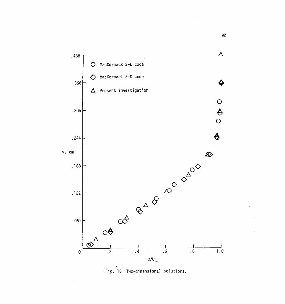
92
·488
() MacCormack 2-D code
<:> MacCormack 3-~ code .366
~ Present investigation
o .305 ~
o
.244
y, cm $
.183 0<:> ~
0 0
.122 is)
~~ <9
.061 ~ O~
~ @
0 .2 .4 .6 .8 1.0
u/U oo
. Fig. 16 Two-dimensional solutions.

93
6.19 cm.
Fig. 17 Physical dimensions of corners.

IV 4
1 Corner shock 2 Internal shock 3 Slip lines 4 Wa 11 shock
4
IV
Fig. 18 Three-dimensional corner flow characteristics.
94

95
Reynolds number used in all other solutions, and the other with a
Reynolds number equal to 3.9 x 10⁶/m (1 x 10⁵/ in .). The physical posi
tion of the right boundary is moved further to the right because the
effects of the shock are too close to the original position. The Mach
number is 3.64 and the Reynolds number except for the one 180 planar
wedge corner is 2.92 x 10⁵/m (7.42 x 10³/ in .). The free stream and
body temperatures are respectively 217 K (390 R) and 607 K (1092 R).
The fluid properties are for air. Solutions are started impulsively
except for the one high Reynolds number solution and are run for
approximately eight characteristic times for a steady state solution.
For the high Reynolds number case, the initial state is that of the
lower Reynolds number solution. A steady state is obtained through
several increments until the higher Reynolds number is reached.
Flow visualization is presented in the form of continuous tone
density distributions and a combination of continuous tones and con
tours for the temperature at x/xl = 0.83. These distributions are
made for this document from color distributions obtained on the Dicomed
Graphics System mentioned in the introduction. Velocity vectors (uxw)
at the first grid point above the flat plate and cylinder surface are
shown to indicate the direction of flow near the base surface.
Velocity vectors (vxw) at x/xL = .83 are shown to indicate the cross
flow velocity field.
The primary observation from this experiment and others is that
the flow is basically conical. Also, the wedge-cylinder flow fields
for the cylinder radius used are very similar to the planar corners

96
for the same wedge angle. For the 0 and 60 wedge angle solutions, the
zones of flow (Fig. 18) described by Charwat and Redekopp [34] are
readily seen (Figs. 19, 20, 21, 22, and 23). That is, for a traverse
plane of a symmetric planar corner, there is Zone I (a region of
conical flow bounded by slip lines and the corner shock), Zone II (a
region of complex flow bounded by slip lines and a strong internal
shock), Zone III (an outer interaction region characterized by a com
pressive fan centered at the triple shock intersection point), and
Zone IV (undisturbed wedge flow). Figure 18 depicts the flow situation
in a symmetric traverse plane. Charwat and Redekopp [34J also concluded
that the flow structure remains qualitatively similar with change in
Mach number for symmetric planar corners, and is distorted without
losing its identity for asymmetric planar corners. The rectangular
corner solution (Fig. 19) shows the zones of flow in a symmetric
pattern. The plate-cylinder corner solution (Fig. 22) is very similar
to the rectangular corner flow. The base surface curvature modifies
the symmetry to some extent, but close to the corner the flow is
almost identical. The temperature distributions for the rectangular
corner and plate-cylinder are very orderly and follow the zones of flow.
As predicted by Charwat and Redokopp [34] the 60 wedge corners
show the zones of flow somewhat distorted (Figs. 20 and 23). Again the
60 wedge-cylinder corner solution is very similar to the 60 planar
corner solution. Also, the 60 corner solutions show two interesting
characteristics that are observed in the larger wedge angle solutions

but not observed for the 00 solutions. The crossflow velocity
separates on the wedge surface about the internal shock.
97
The crossflow velocity separation is observed in all the non~zero
wedge angle cases computed at Reynolds number equal to 2.92 x 10⁵/m
(Figs. 10,21, 23, 24, and 25). The second characteristic is the high
crossflow velocity near the flat plate or cylinder surface under the
internal shock. This phenomenon is observed on all the non-zero wedge
angle solutions.
Cooper and Hankey [38] performed experiments on a 150 asymmetric
planar corner at Mach 12.5. They observed one triple point instead of
the two observed by Charwat and Redekopp [34]. The numberical experi
ment by Shang and Hankey [3J basically confirmed the one triple point
observation. The 12.2 and 180 wedge angle solutions obtained at the
low Reynolds number and described herein appear to show two triple
points although highly distorted. The corner shocks are almost
vertical. The high Reynolds number solution for the 180 wedge angle,
however, indicates that there is only one triple point. In fact, the
high Reynolds number solution is qualitatively very similar to that of
Shang and Hankey [3]. The relevance of Reynolds number is discussed
further at a later point.
Korkegi [48J has described supersonic flow in three-dimensional
corners and associates separation with the shock strength which is a
function of the wedge angle. Both laminar and turbulent corner flow
display the separation phenomenon, however, a larger shock strength is
required to cause separation in a turbulent flow. Korkegi [48]

98
describes three-dimensional separation as a line along which the flow
lifts off a continuous solid surface and three-dimensional reattachment
as a line of flow impingement on a continuous solid surface. Further,
secondary separation can occur when the shock strength is sifficient
for the reverse flow region to separate. The convergence and divergence
of the uxw velocity vectors close to the surface indicate separation
and reattachment. The 0 and 60 wedge angle corner solutions (Figs. 19,
20, 21, and 23) show no strong indication of separation on the plate or
cylinder surfaces. The uxw velocity vectors align themselves with
the direction of the wedge inside the shock and align themselves some
what with shock in the shock region. The 12.20 wedge corner solution
(Figs. 21 and 24) show evidence of convergence of the uxw velocity
vectors or separation, but divergence is not clear.
The 180 wedge corner solution at the lower Reynolds number
(Fig. 25) displays both the convergence and divergence of the uxw
velocity vectors. Figure 26 shows the solution of the 180 wedge corner
at a Reynolds number of 3.9x 10⁶/m (l x 105/in.). The plate surface
pressure (Fig. 27) shows the trough-like pressure variation described
by Korkegi [48J as an indication of secondary separation. The
interesting point about the 180 wedge corner is the effect of
increasing the Reynolds number. Starting with the steady state solu
tion for the low Reynolds number 180 wedge corner solution, the
Reynolds number is gradually increased and a new steady state achieved.
The velocity vectors are rescaled since the velocity is much greater
in magnitude at the same relative position as the low Reynolds number
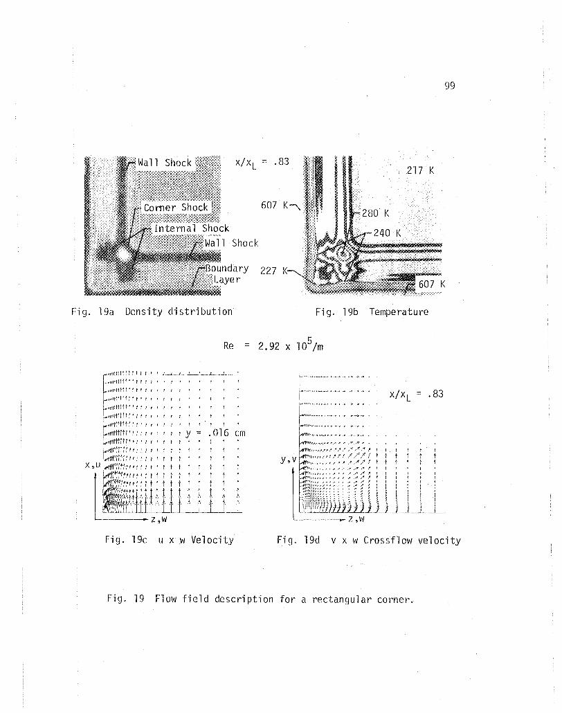
99
.83 217 K
227
Fig. 19a Density distribution Fig. 19b Temperature
tltttllJl!!!! 1 t t .. LL .. J ... _.L L ... 1_ ... L .... .1
",,,,,II!!tll'l! ttl I' "
."""IIltlI11 t ttl I I , , f f x/xL::: .83 ",,,,.tttttttl1: ttl Iff f I I I I
I I I tIt
I I Itt t f
I Itt Y .016 em t t
t X ,u ~tt tt ' ttl Itt t t t t t t t
~.' i I/ttttll ttl t t t t t t t t t
iI 111ft rtf t t t t t t t t t t t t t
· II~mlllijllJll ----z,w
Fig. 19c u x w Velocity Fig. 19d v x w Crossflow velocity
Fig. 19 Flow field description for a rectangular corner.

X/XL::: .83 217 K
275
ce Shock
261
Fig. 20a Density distribution Fig. 20b Temperature
Re :: 2.92 X 10⁵ 1m
I ~!II! II" ! I r t ttl y t
, t
Crossfl ow , t tSeparation
t t
y,v
X/XL::: .83
100
Fig. 20c u X w Velocity Fig. 20d v x w Crossflow velocity
Fig. 20 Flow field description for a 60 wedge-plate corner.

x/ x ::: .83 k L 217 K
311
shock
294 K
Fig. 21a Density distribution Fig. 2lb Temperature
Re ::: 2.92 x 10⁵/m
'Crossflow ,Separation
cm y,v \~
X/XL .83
101
Fig. 21c u X w Velocity Fig. 2ld v X w Crossflow velocity
Fig. 21 Flow field description for a 12.20 wedge-plate corner.

102
Plate Shock X/XL == .83 217 K
Shock
227
Shock
607 K
Fig. 22a Density distribution Fig. 22b Temperature
t t, t t t t
t t t t t t .... _-- ...... - .. x/xL .83 ==
..... -... _----., .. t t t t t t
t t t t t t
t t t
Y ::::
t t t
Fig. 22c u X w Velocity Fig. 22d v X w Crossflow velocity
Fig. 22 Flow field description for a plate-cylinder corner.

X/XL == .83 217 K
273 K K
261 K
607 K
Fig. 23a Density distribution Fig. 23b Temperature
I t
I Itt
t ttl Crossflow I I I I Separati onr--...."r~ ..
~§fffm y,v
'------ Z,w
X/XL == .83
I I I
! I I
Itt I
t /~ / ' , / I
Fig. 23c u X w Velocity Fig. 23d v X w velocity
Fig. 23 Flow field des~ription for a 60 wedge-cylinder corner.
10J

Shock X/XL = .83
217 K
319 K
607 K
Fig. 24a Density distribution Fig. 24b Temperature
Re = 2.92 X 10⁵
/m
Crossflow Separation
y = .016 cm ,!t'f~~"lfrt" I' Ii ;. 1 , tit , ,
t t
• t X,u , .
I
,t t ~\ i' 'I' ,
Y,v , f
I i
'----.... Z,w
X/XL = .83
, , ,
104
Fig. 24c u X w Velocity Fig. 24d v X w Crossflow velocity
Fig. 24 Flow field description for a 12.20 wedge-cylinder corner.

X/XL ::: .83
ock 607
ock 371 K
293 K
Fig. 25a Density distribution
217 K
Fig. 25b Temperature
~~~Y
,~~.~}, •.. ~.?'
. .u.................,... __ ,:~/~;: f;. y,v I ___ "~
Z,w
105
Fig. 25c u X w Velocity Fig. 25d v X w Crossflow velocity
Fig. 25 Flow field description for an 180 wedge-plate corner.

217 K
Shock
347 K
Fig. 26a Density distribution Fig. 26b Temperature
Re ~ 3.9 x 10⁶/m
/ .. / ~~ /"<ri/ /' /' /" .... I'
Y ::: .016 cm '/'/'/"/ ...... f
/'~ , , t t t t t t t t t
t t Y'Vf~~
106
Fig. 26c u x w Velocity Fig. 26d v x w Crossflow velocity
Fig. 26 Flow field description for an 180 wedge-plate corner (high Reynolds number).

4.0
3.6 _
3.2
2.8
2.4
2.0
P 1 ~-
1.6
1.2
.8
c
.4
o
-.4 o .4
Reyno 1 ds n umbe r ::::
3.9 x 10⁶/m (1. x I05/ in )
Reynolds number ::::
2.92 x 10⁵/m (7.42 x 10³/in.)
I I I I I I I " II I I " I I I I II I I I I II II I
.8 z-z 1.2 -w-x
1.6 2.0 2.4
Fi g. 27 Surface pressure for an 180 wedge-p 1 ate corner.
107

108
case. The grid is coarse for defin'ing the boundary layer, but the
solution correlates better with physical experiments than the low
Reynolds number solutions. Only one triple point is observed and
separation, reattachment, and secondary separation are readily seen in
Figure 26 and the surface pressure in Figure 27. Obviously the Reynolds
number is a key parameter in the inviscid-viscid interaction in a three
dimensional corner.
From a qualitative point of view it is apparent that the grids
generated with the "two-boundary technique" perform well for the low
Reynolds number solutions. The surface pressure for the 0, 6, and 12.20
wedge-plate and wedge-cylinder solutions are shown in Figures 28-29.
The surface pressure for the 12.2° wedge-plate corner is later compared
with a solution obtained for the same boundary geometry with a finer
grid.
4.1.1 High Resolution Grid Solutions
It is implied in the above section that more grid points are
needed to resolve the fine structure of supersonic flow about three
dimensional corners at high Reynolds numbers. In this section three
solutions at a high Reynolds number and one at a low Reynolds number
are described where a 12 x 64 x 64 grid is used. The objective of the
section is to present the most highly defined solutions within existing
computational capabilities and further validate the use of the "two
boundary technique." The coordinate transformation presented by Shang
and Hankey [4J is used to compute the solution about a 12.20 symmetric

p 15; -
1.4
1.2
1.0
.8
.6
.4
.2
0
-.2 o
109
6. 6 \ 6.
\ 6. 12.20 Wedge-plate 6.
\ o 60 Wedge-plate 6 o ' Rectangul ar
\ Re = 2.92 x 10⁵/m 6.
\ 6
o \ ~ ~ 6
~ \ °<>.6,
'0.6.-6.-6-6. __ 6. <).'0 '
.2
"<) 6. '<> '6. '<>, ~
DO 0 0'0-0 <>", ""'-.....6 -0-0_ 0" ~
.4
z-z W -x
O-O_.~_
II I I I I I I I I II I I I II II I I
.6 .8 1.0 1.2
Fig. 28 Surface pressure for wedge-plate corners.

no
1.4
1.2
1.0
t::,. 12.2° Wedge-cylinder .8 ~ <> 6° Wedge-cylinder
l::::. 1 0 0° Wedge-cylinder
1 Re::: 2.92 x 10⁵ 1m P .6 1 -- - 1 Pc
\ ~
\ .4
\ , \0 ~ <>00 .2 , 0& D..M~6 .. ~</;
ODD 0.0_ ~\>~ O-O-O~~ .
0 =~O-D
-.2
o .2 .4 .6 z-z .8 1.0
W --x
Fig. 29 Surface pressure for wedge-cylinder corners.

111
wedge-wedge corner (Fig. 30) at Mach 3.64 and Reynolds number
3.9 x 10⁶/m (1 x 10⁵/ in .). The soiution is compared with the experi
mental data obtained by Charwat and Redekopp [34J. Using the Shang-
Hankey transformation which can also be derived with the IItwo-boundary
technique ll and letting one of the wedge angles be zero, the solution of
the flow about a 12.20 asymmetri c wedge corner oj s obta i ned wi th the
12 x 64 x 64 grid. A 12 x 64 x 64 grid is generated using Equation o
(2.17) and a solution is again obtained for the flow about the 12.2
asymmetric corner. The procedure for obtaining solutions at the high
Reynolds number is to first start the solution at a low Reynolds number
and increment to the larger value. The flow conditions are changed on
the upstream plane and are integrated downstream.
The transformation used in [4J is
E;, :: x/xL (3.1a)
n :: 1 ,Q,n [1 + (ek - l)(.l - tan 1 (3.1b) ow) y] k x L
c: :: 1 ,Q,n [1 + (ek - 1)(~ - tan 1 (3.1c) 8) z] . k x L
This transformation can be derived with the "two ... boundary technique ll
where
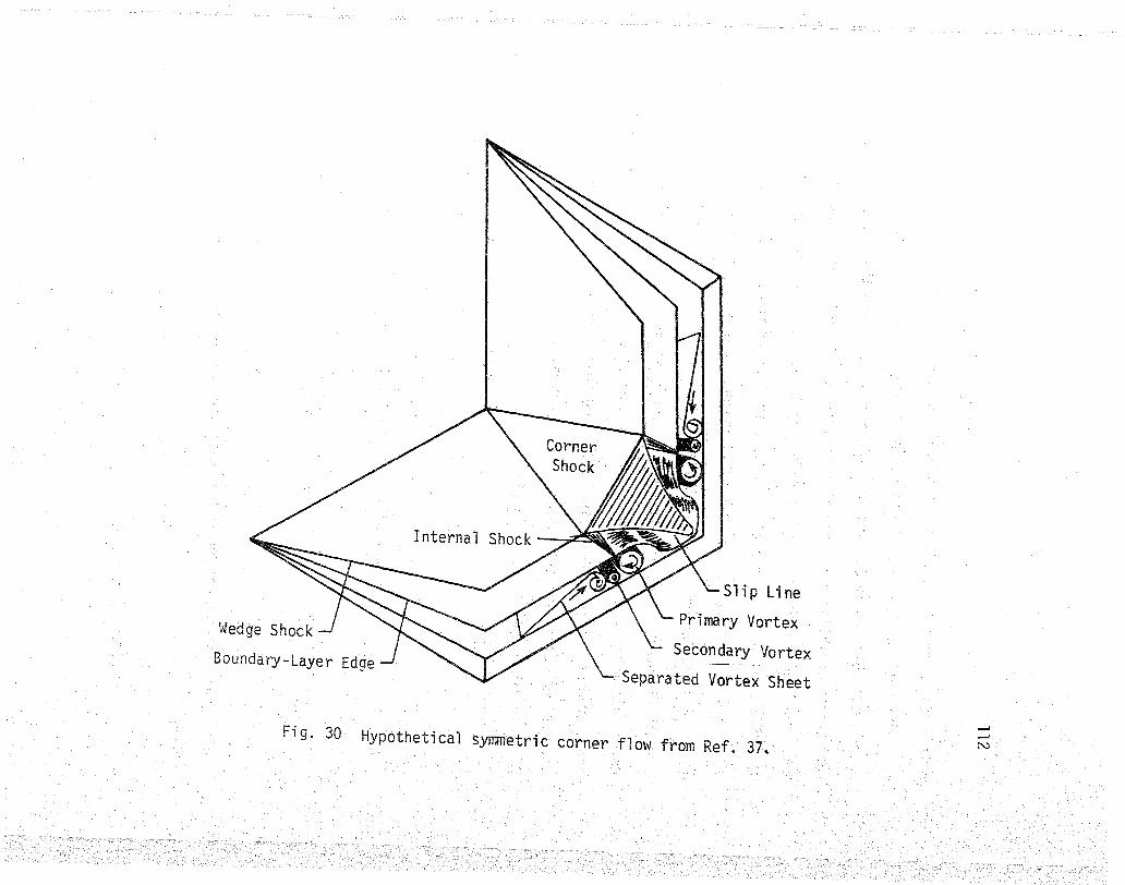
Wedge Shock
Boundary-Layer Edge
Slip Line
Primary Vortex
Secondary Vortex
Separated Vortex Sheet
Fig. 30 Hypothetical symmetric corner flow from Ref. 37, --' --' N

~
- ekL; - 1 L; :: ---.~c.-----'-
ek - 1
Using a linear connecting function and rearranging terms yields
x :: t;, X L
113
(3.2a)
(3.2b)
(3.2c)

114
Equation (3.1) is the inverse of Equation (3.2). This transformation
applies only to corners formed from planar intersecting boundaries, and
the transformation data is derived directly by differentiating ~, n,
and ~ with respect of x, y, and z.
The solution obtained with a 12 x 64 x 64 grid and Equation (3.1)
for a 12.20 symmetric wedge corner is shown in Figure 31-34. The
density and temperature distributions show the zones of flow described
by Charwat and Redekopp [34J. In this solution, the slip lines are
very well defined. The line contour plot (Fig. 32) and the surface
distribution of the density (Fig. 33) also shows the zones of flow and
the rapid change in density associated with the slip lines. The slip
line definition is not ~s apparent for the rectangular corner solution
shown in the previous section. No crossflow separation is observed,
which is the case with the rectangular corner. The position of the
shock structure from [34J is superimposed on the density contour plot
(Fig. 32) and the agreement is good. In [34J the shock structure is
not perfectly symmetric, and only the upper half is used for comparison.
The surface pressure in Figure 34 shows the comparison of the Navier
Stokes solution with Charwat's experiment [34J. The plateau, dip, and
overshoot described by Korkegi [48J occur at nearly the same position.
There is, however, some disagreement in the pressure magnitude. The
Navier-Stokes solution is on the low side. There is pressure dispersion
in Charwat1s data [34J but the pressure magnitude is still larger than
that obtained in the Navier-Stokes solution. Two possible sources for
this difference are (1) the Reynolds number may not be exactly the same

Fig. 31a Density distribution
x x
L.
,,8
Fig. 31b Temperature
6 Re = 3.9 x 101m
115
J Fig. 31c u x w Velocity Fig. 3ld v x w Cross:flm'l Velocity
Fig. 31 Flow field solution for a symmetric 12.20 wedge-wedge corner.

LLLLLll L UJ.L LLU.LU J LLLl J J.J.Lulu JJ.LU u.1LLI J. U .11.Ll ' •. Ll.J.1 J J i iLLUI 1 u. II.! 11J .11 U.U 1 Ll J
o
IJLUJJ.!
o
116
N o M
o


L -1 Pe
1.6
1.4
1.2
1.0
.8
.6
.4
.2
o
Data from Ref. 34 ~/~ Spread, of experimental data
/
0
000 cP b
o Navier-Stokes solution
6 Re = 3.9 x 101m
cP '0 o /
o \ o
\ 0,
00'0-0-0-0-0
-.2 ~LU~~~~~~I~II~I~I~II~I~II~I~I~~II~I~I~II~IJI_~II~I~I~II~I~II~L_LI~II~I~I~II~I~I~"~II o .2 .4 .6 .8 1.0 1.2
z-zW x
Fig. 34 Surface pressure for a 12.20 symmetric corner.
118

119
in the numerical and physical experiments~ or (2) the pressure damping
in the numerical technique may be retarding the pressure magnitude.
The plateau region (Fig. 34) is associated with the relatively low uxw
velocity vectors in Figure 31 and the separated region. The separation
line is under the plateau near the undisturbed flow and reattachment
occurs at the high pressure rise and where there is corresponding large
velocity vectors.
The dip in the pressure curve is associated with secondary separa
tion as described by Korkegi [48J. This secondary separation region is
shown in the density contour plot (Fig. 32) and there are closed con
tour lines which indicate vortical motion as described by Watson [37J.
However, the author has 'not observed vortical motion in the velocity
data.
It is evident that the 12 x 64 x 64 grid derived from Equation
(3.1) allows for the definition of the fine structure of the flow. The
solution obtained with the Navier-Stokes solver is in good comparison
with the corresponding experiment. The possible concentration of more
grid points in the secondary separation region may be desirable but
would not work well with Equation (3.1) because of its exponential
characteristics.
Following the solution for a symmetric planar corner flow, super-
sonic flow about an asymmetric corner is obtained by letting the wedge
angle ~w in Equation (3.1) on the bottom surface be zero. The wedge
angle 8w remains 12.2° and the 12 x '64 x 64 grid for this corner is
generated with Equation (3.1). The Navier-Stokes solver is applied

120
with the transformation startj 5i with a low Reynolds
number and incrementing to 3.9 x 10b/rn. The solution is shown in Fig-
ure 35-38, but is not compared to a physi experiment. The solution
obtained with a grid generated using Equation (2.17) is compared to
this solution.
For the asymmetric corner and the 12 x 64 x 64 grid only one
triple point is observed. However$ the internal shock from the wedge
generates a very similar flow pattern as in the symmetric corner near
the bottom surface. The pattern is, however, closer to the wedge sur
face since there is no corner shock. The crossflow separation is
observed at the high Reynolds number but is relative weak compared to
the lower Reynolds number solutions.
Equation (2.17) is used to'generate a 12 x 64 x 64 grid with the
previously used physicalrlirOOtlstons and contraction parameters
kl = k2 = 2.9. The transformation data for the grid is applied in the
Navier-Stokes solver in the same manner as before. The surface pressure
for the solution at Reynolds number 2.92 x 10⁵/m is shown in Figure 39
and compared with that obtained with the 20 x 36 x 36 grid. The agree
ment is good where the grid is dense and the solution at Reynolds
number 3.9 x l06/m is obtained through a series of increments. This
solution is presented in Figures 40-43. The surface pressure in
Figure 43 is compared to that obtained with the grid defined with
Equation (3.1). Overall the agreement is good. One point that is
noticed, however, is that the shock i.s more smeared in the solution
obtained with the transformation data from Equation (2.17). This is

Fig. 35a Density distribution
xl = .8 xL
607 K
Fig. 35b Temperature
6 Re - 3.9 x 101m
121
Fig. 35c u x w Velocity Fig. 35d v x w Cross flow velocity
Fig. 35 Flow field description for a 12.20 asymmetric corner (12 x 64 x 64 grid-exact boundaries)

y-yw --x .5
.4
.3
.2
. 1
0
1°~~l
6 Re = 3.9 x 101m
=----:-==::
122
I, , " , , , , , I" , , , , , , ,I, , , , "llLlJ..LlLLLllLLLLLLLLLU.llLLLLUlLlulilJ.J...ulllLUJ_LLLLLL.llLL1.lll, , , , , , , , , I
o .1 .2 .3 .4 .5 .6 .7 .8 .9 1.0
x
Fig. 36 Line contour plot of 12.20 asymmetric corner (12 x 64 x 64 grid-exact boundaries).

123
6 Re = 3.9 x 10 /m
Fig. 37 Perspective view of distribution of density for 12.20 asymmetric corner x/xL = .8 (12 x 64 x 64 grid -exact boundaries).

2.2
1.8
1.4
1.0
.6
. 2
-.2 o.
\ o
\ o
\
6 Re = 3.9 x 101m
o
\ 0'
\ o \ c:Fb=DODODDD 0 O .
~ 0'0'0 "'0-0-0-0
1IIIIIIIIIIIIIIIIIIIIIIIIIIIIIUJLWill uJ .2 .4 .6 .8 1.0
Z-Zw x
Fig. 38 Surface pressure for 12.20 asymmetric corner (12 x 64 x 64 grid - exact boundaries).
124

2.2
1.8
1.4
p P .. 1
e
.2
[J 20 x 36 x 36 grid
o 1 2 x 64 x 64 g rid
,~ ~~<>::--D
"'(>0.-. ~O,~
11111111111111111111111111111111.11111111111 -.2~~~~~~~~~~~~~~~~_U-~~
o .2 .4 .6 .8 1.0
Fig. 39
--x
Surface pressure comparison for grid refinement at Re = 2.92 x 10⁵/m.
125

607 K
Fig. 40a Density distribution
Re = 3.9 x 10⁶/m
X,u
, " f r r t t t
:///, /,////,/ ,,1/ /I Itt t t t t
~.,-'fllrttttttt t t t
z,w
126
Fig. 40b Temperature
Fig. 40c u x w Velocity Fig. 40d v x w Crossf10w velocity
Fig. 40 Flow field description for a 12.20 asymmetric corner (12 x 64 x 64 grid - approximate boundaries).
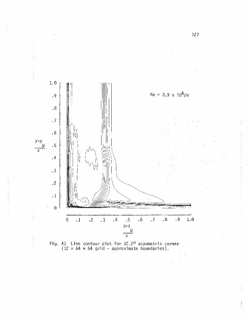
y-y __ tv
x
127
1.0
~ .9 I
~ I I II
.8 Ilili 'II
;11
.7 II 'i[1
.6 III/ III) I·
II .5 II
Q I1I1
.4 i ~
.3
.2
.1
0 s::-------
I I I I I I I I I I I I I I uUDlu.l.llLJ ill-LLLLLLl.LJ.iu.u..1.Ll..LLLu..LU l.J..l..l.l.u..L.I.LU.iu...u.l.LH.LU.D.Ll.DllLuLlluill
o .1 .2 .3 .4 .5 .6 .7 .8 .9 1.0 z-z
H --x
Fi g. 41 Line contour plot for .12 ~2° asymmetri c corner (12 x 64 x 64 grid - approximate boundaries).

128
Re = 3.9 x l06/m
Fig. 42 Perspective view of distribution of density for 12.20 assymmetric corner x/xL = .8 (12 x 64 x 64 grid -approximate boundaries).

129
2.2 0 Eq. 3.1
<> Eq. 2.7
1.8
~ Re = 3.9 x 10⁶/m
1.4 \ P 1.0 --1 Pe
.6 t ~ .2
~6~~~~
-.2 0 .2 .4 .6 .8 1.0
z-zW --x
Fi g. 43 Comparison of surface pressure for two different grids.

130
attributed to the growth of the transverse mesh distribution in the
windward direction. Using Equation' (3.1) there is a very fine grid
upstream and the grid becomes coarser with the expanding flow down
stream. Using Equation (2.17) the grid is coarse upstream and is finer
at the downstream positions.
It is concluded that the "two-boundary technique" in viable for
computing grids about three-dimensional corners where the Navier-Stokes
equations can be applied to compute supersonic flow. It is noted, how
ever, that if only planar intersecting corners are of interest, Equa
tion (2.17) is not the optimal application of the technique. Planar
intersecting corners are approximated using Equation (2.17). Neverthe
less, the "two-boundary.technique" is highly versatile and affords a
great deal of flexibility.
4.2 Supersonic Flow About Spike-Nosed Bodies
Spike-nosed configuration occurs in many supersonic flow situa
tions. Unlike the three-dimensional corner flows that are studied
herein, the flow fields about spike-nosed bodies can be highly unsteady.
The unsteadiness manifests itself as self-sustained oscillations which
have been observed for a wide variety of shear-layer impingement con
figurations [49J. Two spike-nosed bodies are examined in this section:
(1) a body with a small nose length to should height ratio (0.71); and
(2) a body with a large nose length to shoulder height ratio (2.14).
These two configurations have been examined by Shang, Hankey, and
Smith [50J. The first two authors posed the problem and this author

131
applied the IItwo-boundary technique" to generate the grids and obtained
the initial solutions with the Navier-Stokes solver. The emphasis
herein is on the application of the "two-boundary technique" for grid
generation about the spike-nosed bodies. The "two-boundary technique"
has been used to generate grids using a linear approximation to the
body surface, a circular arc outer boundary, and a linear connecting
function. A parabolic algebraic function and an exponential function
are used to concentrate the grid in the nose shoulder region. The
details of the application of the "two-boundary technique" to these
geometries are developed in Chapter 2 along with the derivatives for
the transformation data. The three-dimensional Navier-Stokes solver
is used to obtain the numerical solutions to the flow fields. For
these solutions the z-coordinate direction is the windward direction.
An axisymmetric solution is obtained by the rotation of the grid about
the z-axis and solving the three-dimensional equations of motion. The
argument for this approach rather than developing an axisymmetric
solver is the considerable time savings compared to the programming a
specific code for this problem. These solutions demonstrate the versa
tility of the Navier-Stokes solver.
4.2.1 One-Half-Inch Spike-Nosed Body
The spike-nosed body with the small ratio of nose length to
shoulder height has a nose length of 12.5 mm (0.5 in.) and a shoulder
height of 19.05 mm (0.75 in.). The boundary surface for this body is
shown in Figure 9 and the grid generated with the "two-boundary

132
technique" is shown in Fi gure 11. The data used to generate the gri d
is found in Table 2. Figure 44 shows the density distribution of the
developing flow. A relatively low density region compared to the sur
roundings develops at the top of the nose and later sheds off the
shoulder. After this point only low amplitude oscillations occur in
the nose-shoulder region. Plots of pressure along three lines of the
grid (Fig. 45) are shown after 4000 time steps in Figures 46-48.
Two modifications to the data for generating the grid for the one
half-inch spike-nosed body are performed and the solutions recomputed.
The objectives of the modifications are to assure the validity of the
grid generation technique.
The first modification is a change in the concentration of grid
points. The new grid is obtained by making the constant k = 3 instead
of 2.2 in Table 2. This means that there are fewer grid points to
define the shock in the radial direction and more points near the inner
boundary. Figures 49-51 show the pressure comparison with the original
case at the 4000th time step for the three lines. The second modifica
tion moves the outer boundary closer to the inner boundary concentrating
more points in the shock region. The radius of the circular arc defining
the outer is changed from 13.26 mm (0.522 ft) to 12.55 mm (0.494 ft) and
the constant k is set equal to 1.75 so that the distance of the
nearest grid point to the inner boundary is approximately the same as
that in the original case. Figures 52-54 show the density comparison
with the original case and the first modification. It is seen from the
plots that there is overall good agreement. The differences that exist

133
~ '"Cl 0
..Cl
'"Cl <J.J 1Il 0 c: I
<J.J ~ 'r-0..
('I'") 1Il
...c.: u c:
'r-
4-r--
CO ...c.:
I <J.J s::: 0
S-O
4-
s::: 0
'r-+-> :::I
r--0 1Il
>, +J 'r-1Il s::: OJ
'"Cl
4-0
+-> s::: OJ E 0.. 0
OJ > OJ Cl
o:::t o:::t
O'l 'r-LL.

1
Fig. 45 Grid lines for quantative comparison one-half inch spike-nosed body.
134

135
• 1
. +..l '+-
r-- .01 8 0 8
OJ s:::::
~ .,....
0')
s::::: 0 0 r-- 0 res
OJ 0 U s::::: 0 res +..l V)
0 0 .001
0
o. 1. 2. 3. 4. x 10-5
Dens i ty $ Sl ug/ft. 3
Fig. 46 Density along line one for base case.

136
• 1
..fJ If-
'" O"'l N
OJ C
.01 'r- B C')
c c:J 0 r--co c:J OJ c:J u c co
..fJ c:J (/)
'r-a
c:J
.001
O. 1. 2 . 3. 4. x 10-5
Dens i ty it Sl ug/ft. 3 I
Fig. 47 Density along line twenty-nine for base case.

137
• 1
. +-> 4-
'" M LO
OJ s::
,......
Ol .01 s:: 0 ,...... n:s OJ u s:: n:s
+-> Vl
.r-0
<)
.001
o. 1. 2. x 10-5
Density, Slug/ft. 3
Fig. 48 Density along line fifty-three for base case.

. ...., 4-
...-OJ s::: 'r-..... (j) s::: 0 r-res OJ U c: res ...., Vl
'r-0
0 Base Case
0 New Solution
<) .01 0
{} <)
.001 @
<8
<>
o. l. 2. 3. 4. x 10-5 ,
Density, Sl ug/ft. 3
Fig. 49 Comparison of density solution for grid concentration change line = 1.
138

• ..f..J 4-
.. 0'1 N
(]) s:: 'r-
0'> s:: 0 ,...... co (]) u s:: co
..f..J Vl
'r-0
• 1
.01
.001
o. 1. 2. 3.
Density, Slug/ft.3
o Base Case
<> New Solution
-5 4. x 10
Fig. 50 Comparison of density solution for grid concentration change line = 29.
139

• 1
• 0 ...., Base Case tf-
'" <> New Solution M U')
Q) s:: 'r-
.01" r--
Ol
§ r--ttS
Q) U s::
<) ttS ...., V'I
$ 'r-0
8 .001
<)
o. 1. 2. x 10-5
Density, Slug/ft. 3
Fig. 51 Comparison of density solution for grid concentration change line= 53.
140

. 01
• +l 4-
(]) c:
c::n c: 0 .--to
(]) u .001 c: to +l Vl 'r-0
<> 0
Base Case New Solution
B $
&
<8
~ ______ ~ ______ ~ ________ ~_______J 4. x 10-5 O. 1. 2. 3.
Density, Slug/ft. 3
141
Fig. 52 Comparison of density solution for outer boundary change 1.

. ..f-l 4-
'" (j)
N
OJ s:::
0) s::: 0 ,....... co OJ u s::: co
..f-l V')
'r-a
• 1
00
.01
.001
O. l. 2. 3.
Density, Slug/ft. 3
142
o Base Case
<> New Solution
<0 <) @
8 0
4. x 10-5
Fig. 53 Comparison of density solution for outer boundary change line = 29.

. 4-l I+-
... M 1.0
CU C
''''' 0> c 0 ,.... rt::I
CU U C rt::I 4-l til .,...
0
• 1
.01
.001
0
8
o Base Case 0- New Solution
o. 1. 2. x 10-5
Dens i ty, S1 ug/ft. 3
Fig. 54 Comparison of density solution for outer boundary change line = 53.
143
144
are due to the grid spacing in the shock region and inner boundary
region. The shock is more smeared when there are fewer grid points in
that region and the placing of grids points closer to the inner boundary
affects the accuracy there. No attempt is made here to analyze the low
amplitude oscillation for the one-half-inch spike-nosed body_ It is
seen that the perturbed grids produce good agreement with the original
case and, this is an indication that the grid generation technique is
viable for this application.
4.2.2 One and One-Half-Inch Spike-Nosed Body
The spike-nosed body with the large ratio of nose length to
shoulder height has a nose length of 38.1 mm (1.5 in.) and a shoulder
height of 19.05 mm (0.75' in.). The body surface for this configura
tion is shown in Figure 10 and the grid generated with the "two
boundary technique" is shown in Figure 12. Table 3 contains the data
used to generate the grid. Table 3 is the same as Table 2 except the
nose length is one inch longer and the outside circular arc is longer.
The Navier-Stokes solution for this grid and initial conditions pro
duces high amplitude oscillation. The characteristics of the oscilla
tion can be seen from experimental observation. Figure 55 shows a
sequence of shadowgraph pictures [51J of a spiked-nosed body flow
field in one cycle of oscillation. After the initial transient, the
bow shock interact with the shock from the shoulder near the top of the
shoulder. A strong reverse flow occurs between the shock and the
boundary forci ng the shock to bul ge ou't. Wi th the shock bul ged out,

145
Fig. 55 Shadowgraphs of oscillating flow field.

146
the high energy fluid behind the shpck along with shock is forced
downstream by the outer flow until the bow shock again interacts with
shoulder shock. The cycle r'epeats itself. This phenomena is also
shown by Harney [52J for blunt nosed bodies which is approximated by
the one and one-ha1f-inch spike-nosed body. Widhopf [53J has shown
the oscillating phenomena over indented nose tips while numerically
solving the Navier-Stokes equations. Figure 56 shows a sequence of
density distributions for one cycle taken from the numerical solution.
The phenomenon described above is observed in the numerical solution of
the flow about the one and one-half-inch spike-nose body. The cycle
repeats itself and maintains its form. The oscillation phenomenon is
independent of Reynolds number [50J but is dependent on the speed of
sound which in turn depends on the free stream temperature. The pri
mary frequency is 3100 cycles/sec where the free temperature is 217 K
(290 R). In [51J using a Reynolds number of 7.78 x 10⁶/m and free
stream temperature of 111 K (200 R) a lower primary frequency of
2665 cycles/sec is observed. The pressure at approximately point 29
(Fig. 48) and the observed pressure from an experiment conducted at the
Wright-Patterson Flight Dynamics Laboratory are shown in Figure 57. It
is seen in the figure that the wave form and frequency from the experi
ment and the numerical solution are in good agreement.
The IItwo .. boundary technique" for grid generation has been success
fully applied for two spike-nosed bodies. The Navier-Stokes solver has
produced unsteady numerical solutions for several initial conditions

Fig. 56 Density distribution during one cycle of oscillation for one and one-half inch spike-nosed body_
..p:. '-J

Spike wave form 20 __ ------------------------------------------------~
Computation 10
8 0.. ........ 0..
~ oJiillilililii~'J~;;;;;;;;;;;;;;;;;;;;~::~::======~~~~--~~~ ~ 20 ~ ~ ~ ~
0..
10
o 1 2
Time level
Figure 57.- Surface pressure on one and one-half inch spike-nosed body_
3
+::> OJ

149
with Reynolds numbers up to 7.78 x 10⁶jm. Overall, the solutions that
have been obtained simulate the observed phenomena very well.
5. CONCLUS IONS
An algebraic grid generation technique has been developed and
explored in conjunction with the solution of the compressible three
dimensional Navier-Stokes equations. The technique called the "two
boundary technique" is simple to understand, easy to apply, and has a
high degree of generality for the finite difference solution of complex
flow field problems. The "two-boundary technique" allows direct control
of a grid and direct computation of the Jacobian derivatives.
The viability of the grid generation technique is demonstrated
through the development and application of a Navier-Stokes solver which
operates on the CDC CYBER-203 vector computer. The computer program is
based on a MacCormack time-split technique which is chosen because of
its compatibility with vector computer architecture. The finite differ
ence algorithm is written in the SLjl programming language, and the
32-bit word length arithmetic and storage option is used. This option
doubles the number of grid points that can be used for a given amount
of memory and approximately doubles the computational rate as compared
to the normal 64-bit words. Using SLjl and the halfword option the
computational rate is 4 x 10⁻⁵ seconds per grid point per time step,
and solutions with 5 x 10⁴ grid points can be obtained without using
secondary memory. It is concluded from the numerical experiments
presented in the present study that the 32-bit word length is adequate

150
when solving the Navier-Stokes equations for supersonic laminar flow
using an explicit MacCormack technique.
Complex supersonic flow field solutions are obtained for two dis
tinctly different geometries using the IItwo-boundary technique ll for
grid generation and the Navier-Stokes solver. First, supersonic flow
solutions about a family of three-dimensional corners are obtained . . ,
These flow fields reach a steady state but are characterized by strong
shocks and three-dimensional separation. The Mach number is 3.64,
Reynolds numbers are 2.72 x 10⁵/m and 3.9 x 10⁶/m, and the fluid proper
ties are for air. It is shown that the solutions obtained agree well
with physical experiments and other numerical experiments. Also,
corner flow solutions with 5 x 10⁴ grid points are among the most
refined Navier-Stokes solutions obtained to date. The second flow
situation is supersonic flow about spike-nosed bodies. In this case,
the flow is axisymmetric, unsteady, and characterized by a strong bow
shock and massive separation. The Mach number is 3 and the Renolds
number is 7.78 x 10⁶/m• The numerical solutions show dramatically the
oscillating flow generated by the interaction of the bow shock and
shoulder wall of the body. The surface pressure and oscillation fre-
quency compare very well with corresponding wind tunnel experiments.
The successful numerical solution of the flow fields support the primary
conclusion that the IItwo-boundary technique ll is viable for generating
grids for complex flow field solutions. Also, for the spike-nosed
bodies, considerable development time for a specialized axisymmetric
code is saved.

151
Plans for the use of the "two-boundary technique" include develop
ment of grids with wing-fuselage boundaries, analysis of non-orthogonal
grids, development of additional spike-nosed body grids, and the
development of numerical grid control functions.

152
REFERENCES
1. MacCormack, R. W.; and Lomax, H.: "Numerical Solution of Compressible Viscous Flows." Annual Review Fluid Mechanics, 1979, Vol. 11, pp. 238-316, Annual Reviews, Inc.
2. HacCormack, R. W.; and Paullay, A. J.: "Computationa1 Efficiency Achieved by Time Splitting of Finite Difference Operators. II AIAA paper 72-154, Jan. 1972~
3. Shang, J. S.; and Hankey, W. L.: "Numerica1 Solution of the Navier-Stokes Equations for a Three-Dimensional Corner." AIAA paper 77-169, Los Angeles, CA, also AIAA Journal, Vol. 15, Nov. 1977, pp. 1575-82.
4. Shang, J. S.; Hankey, W. L.; and Petty, J. S.: "Three-Dimensional Supersonic Interacting Turbulent Flow Along a Corner." AIAA 78-1210, Seattle, WA, July 1978.
5. Control Data Corporation: "Contro1 Data CYBER-200 Model 203 Computer Hardware Reference Manua1." Publication Number 60256010, Hay 1979.
6. Thompson, J. F.; Thames, F. C.; and Mastin, C. W.: "Automatic Numerical Generation of Body-Fitted Curvilinear Coordinate Systems for Fields Containing Any Number of Arbitrary TwoDimensional Bodies." Journal of Computational Physics, Vol. 15, July 1974, pp. 299-319.
7. Thames, F. C.; Thompson, J. F.; Mastin, C. W.; and Walker, R. L.: "Numerical Solutions for Viscous and Potential Flow About Arbitrary Two-Dimensional Bodies Using Body-Fitted Coordinate Systems. II Journal of Computational Physics, Vol. 24, 245, July 1977, pp. 245-273.
8. Thompson, J. F.; Thames, F. C.; and Shanks, S. P.: "Use of Numeri ca lly Generated Body-Fitted Coordi nate Sys terns for Sol utions of the Navier-Stokes Equations." Proceeding of AIAA 2nd Computer Fluid Dynamics Conference, Hartford, CT, July 1975.
9. Thompson, J. F.; Thames, F. C.; and Mastin, C. W.: "BoundaryFitted Curvilinear Coordinate Systems for Solution of Partial Differential Equations on Field Containing Any Number of Arbitrary Two-Dimensional Bodies." NASA CR-2739, July 1977.
10. Mastin, C. W.; and Thompson, J. F.:- "Elliptic Systems and Numerical Transformations. II Journal of Mathematical Analysi~ and Applications, Vol. 62, Jan. 1978, pp.152-62.

153
11. Coon, S. A.: "Surfaces for Computer-Aided Design of Space Forms." MAC TR-41 (Contract No. AF-33.( 6000-42859) MIT, June 1967. Available from DOC as AD 663504.
12. Gordon, W. J.: "Free-Form Surface Interpolation Through Curved Networks. II General Motors Research Report (GMR 921), Sept. 1969.
13. Gordon, W. J.; and Hall, C.: "Construction of Curvilinear Coordinate Systems and Applications to Mesh Generation." International Journal for Numerical Methods In Engineerin[, Vol. 7, July 1973, pp. 46l-4iT. -
14. Eiseman, P. R.: "Three-Dimensiona1 Coordinates About Wings." Proceeding of the AIAA 4th Computer Fluid Dynamic Conference, Williamsburg, VA, July 1979.
15. Eiseman, P. R.: "A Multi-Surface r~ethod of Coordinate Generation. II
Journal of Computational Physics, Vol. 33, Oct. 1979, pp. 118-150.
16. Eiseman, P. R.: "Geometric Methods in Computational Fluid Dynami cs. II ICASE Report 80-11, April 1980.
17. Schwiekert, D.: "An Interpolation Curve Using Splines in Tension." Journal of Mathematics and Physics, Vol. 45, Sept. 1966, pp.312-317.
18. Cline, A. K.: "Scal er- and Planar-Valued Curve Fitting Using Splines Under Tension." Communications of the ACM, Vol .. 17, No.4, April 1974, pp. 218-233. - -- -- .
19. Pruess, S.: "Properties of Splines in Tension." Journal of Approximation Theory, Vol. 17, Aug. 1970, pp. 86-96.
20. SL/l Reference Manual, Analysis and Computation Division, NASA Langley Research Center, Hampton, VA.
21. Schlichting, H.: Boundary Layer Theory, McGraw-Hill, 1968.
22. Vincenti, W. G.; Kruger, C. H.: Introduction to Physical Gas Dynamics, John Wiley & Son, Inc., 1965.
23. Smith, R. E.; and Weigel, B. L.: "Ana1ytic and Approximate Boundary Fitted Coordinate Systems for Fluid Flow Similation." AlAA Paper 80-0192, Pasadena, CA, Jan. 1980.
24. Dagundji, J.: Topology, Allyn and Bacon, 1968.
25. Ahlberg, J. H.; Nilson, E. N.; and Walsh, S. L.: The Theory of Splines and Their Applications, Academic Press, Inc., 1967.

26. MacCormack, R. W.: liThe Effect of Viscosity in Hypervelocity Impact Crateri ng. II AIM Paper 69-354, May 1969.
27. Roach, P. J.: IIComputational Fluid Dynamics. 1I Hermosa Pub 1 i shers, 1972.
154
28. Holst, T. L.: IINumerical Solution of Axisymmetric Boattail Flow Fields with Plume Simulators. II AIAA Paper 77-224, Jan. 1977.
29. MacCormack, R. W.: IIAn Efficient Numerical Method for Solving the Time-Dependent Compressible Navier-Stokes Equations at High Reynolds Number.1I Computing in Applied Mechanics, ADM, Vol. 18, New York Society of Mechanical Engineering, June 1973.
30. Shang, J. S.: IIImplicit-Explicit Method for Solving the NavierStokes Equations. 1I AIM Journal, Vol. 16, No.5, May 1978, pp. 495-502. --
31. MacCormack, R. W.; and Baldiwn, B. S.: IIA Numerical Method for Solving the Navier-Stokes Equations with Application to Shock Boundary Layer Interactions. 1I AIAA Paper 75-1, Jan. 1975.
32. Smith, R. L; and Pitts, J. I.: liThe Solution of the ThreeDimensional Compressible Navier-Stokes Equations on a Vector Computer. II Third IMAC International Symposium on Computer Methods for Partial Differential Equations, Lehigh University, PA, June 1979.
33. Lambiotte, J. J.: IIEffects of Virtual Memory on Efficient Solution of Two Model Problems. 1I NASA TM X-35l2, July 1977.
34. Charwat, A. F.; and Redekopp, L. G.: IISupersonic Interference Flow Along the Corner of Intersecting Wedges. 1I Men. RM-4863-PR (Contract No. AF49(638)-1700), RAND Corp., July 1966.
35. Stainback, P. C.: IIAn Experimental Investigation at a Mach Number of 4.95 of Flow in the Vicinity of a 900 Interior Corner Alined with the Free-Stream Velocity.1I NASA TN D-184, Feb. 1960.
36. Stainback, P. C.: "Heat-Transfer Measurements at a Mach Number of 8 in the Vicinity of a 900 Interior Corner Alined with the Free-Stream Velocity. II NASA TN D-2417, Aug. 1964.
37. Watson, R. D.: IIExperimental Study of Sharp- and Blunt-Nose Streamwise Corners at Mach 20. 11 NASA TN D-7398, April 1974.
38. Cooper, J. R.; and Hankey, W. L.: "Flow Field Measurements in an Asymmetric Axial Corner at M = 12.5. 11 AIAA Journal, Vol. 12, Oct. 1974, pp. 1353-1357.

155
39. Kulter, P.: "Numerica1 Solution for the Inviscid Supersonic Flow in the Corner Formed by Two I.ntersecti ng Wedges. II AIM Paper 73-675, Palm Springs, CA, July 1973.
40. Shankar, V.; Anderson, D.; and Kulter, P.: "Numerical Solutions for Supersonic Corner Flow. II Journal of Computational Physics, Vol. 17, Oct. 1975, pp. 160-180.
41. ~1arconi, F.: "Supersonic, Inviscid, Conical Corner F1owfie1ds." AIAA Journal, Vol. 18, Jan. 1980, pp. 78-84.
42. Wei nberg, B.; and Rubi n, S.: "Compress i on Corner Flow. II Journal of Fluid Mechanics, Vol. 56, Part 4, May 1975, pp. 753-774.
43. Ghia, K.; and Davis, R.: i'A Study Compres~;ib1e Potential and Asymptotic Viscous Flows for Corner Regions." AIAA Journal, Vol. 12, March 1974, pp. 355-359.
44. Hung, C.; and MacCormack, R.: "Numerica1 Solution of Supersonic Laminar Flow Over a Three-Dimensional Compression Corner." AIAA Paper 77-694, June 1977.
45. Hung, C.; and MacCormack, R.: "Numerica1 Solution of ThreeDimensional Shock Wave and Turbulent Boundary Layer Interactions." AIAA Journal, Vol. 16, Oct. 1978, pp. 1090-1096.
46. Horstman, C.; and Hung, C.: "Computation of Three-Dimensional Turbulent Separated Flows at Supersonic Speeds." AIAA Paper 79-0002, Jan. 1979.
47. Smith, R. L: "Numerica1 Solutions of the Navier-Stokes Equations for a Family of Three-Dimensional Corner Geometries. II AIAA Paper 80-1349, July 1980.
48. Korkegi, R.: liOn the Structure of Three-Dimensional Shock-Induced Separated Flow Regions." AIAA Journal, Vol. 14, No.5, May 1976, pp. 597-600. --
49. Rockwell, D.; and Nandascher, E.: "Se1f-Sustained Oscillations of Impinging Free Shear Layers. II Annual Review of Fluid Mechanics, Vol. II, 1979, pp. 67-94, Annual Review, Inc.--, Palo Alto, CA.
50. Shang, J. S.; Hankey, W. L.; and Smith, R. L: "Flow Oscillations of Spike-Tipped Bodies." AIAA Paper 80-0068, Jan. 1980.

156
51. Butz, J. S.: "Hypersonic Aircraft Will Face Technical Cost Problems. II Aviation Week Including Space Technology, Vol. 70, No. 25, June 1959, pp. 156-169.
52. Harney, D. J.: "Oscillating Shocks on Spike Nose Tips at Mach 3." AFFDL-TM-79-9-FX, Air Force Flight Dynamics Laboratory, WRAFB, Ohi 0, 1979.
53. Widhopf, G. F.; and Voctoria, K. J.: "Numerical Solution of the Unsteady Navier-Stokes Equations for the Oscillatory Flow Over a Concave Body. II Lecture Notes in Physics, No. 35, June 1974, Springler-Verlag, pp. 431-444.

.--------------...--------------,.-----------------"' 1. Report No. 2. Government Acce5sion No. 3. Recipient's Catalog No"
NASA T~1-83123
4. Title and Subtitle 5. Report Oat!'
Two-Boundary Grid Generation for the Solution of ~_M_a~y~1_9-8-1--------~ the Three-Dimensional Compressible Navier-Stokes 6. Performing Organization Cod" I Equations I
505-31-83-02 ! ~------------------------------------------------_r~~~~~~-----------I
7. Author(s) 8. Performing Organizdtion Report No. ! R. E. Smith
...------------------------------1 10_ Work Unit No. -, I 9. Performing Organization Name and Address
NASA Langley Research Center Hampton, VA 23665
1 I- Contract or Grant No.
~--~---------------------,-----~ 13. Ty~~ Repon~dP~~dCov~~ 12. Sponsoring A~r>cy Name and Address
National Aeronautics and Space Administration Washington, DC 20546
15. Supplementary Notes
Technical Memorandum 14_ Sponsoring Agency Code
This report is a dissertation submitted to Old Dominion University for partial fulfillment of the requirements for the Degree of Doctor of Philosophy in Mechanical Engineering. I r-----~~------------~~----~------------------------------1
16. Abstract A grid generation technique called the "two-boundary technique" ",I
is developed and applied for the solution of the three-dimensional Navier-Stokes equations. The Navier-Stokes equations are transformed from a cartesian coordinate system to a computational coordinate system, and the grid generation technique provided the Jacobian matrix describing the transformation.
The "two-boundary technique" is based on algebraically defining two distinct boundaries of a flo.w domain and joining these boundaries with either a linear or cubic polynomial. Control of the distribution of the I grid is achieved by applying functions to the uniform computational grid , which redistribute the computational independent variables and consequently concentrate or disperse the grid points in the physical domain.
The Navier-Stokes equations are solved using a MacCormack time-split technique. The technique is programed for the CYBER-203 computer in the SLjl language and uses 32-bit word arithmetic. Two distinct flow field problems are solved using the grid generation technique and the NavierStokes solver (computer program). Grids and supersonic laminar flow solutions are obtained for a family of three-dimensional corners and two spike-nosed bodies. The "two-boundary technique" is demonstrated to be viable for grid generation associate with supersonic flow. The technique is easy to apply and is applicable to a wide class of geometries.
17. Key Words (Suggested by Authods))
computational fluids, grid generation, supersonic flow
18. Distribution Statement
Unclassified - Unlimited
Subject Category 64
1 9, S~urity Oassif. (of this reportl
Unclassified 20. Security Classif. (of this page)
Unclassified 21- No. of Pages
172
• For sale by the National Technical Information Service, Springfield. Virginia 22151
A08

End of Document