types of machine learning algorithms - cdn.intechweb.orgcdn.intechweb.org/pdfs/10694.pdf · types...
TRANSCRIPT
Types of Machine Learning Algorithms 19
Types of Machine Learning Algorithms
Taiwo Oladipupo Ayodele
X
Types of Machine Learning Algorithms
Taiwo Oladipupo Ayodele University of Portsmouth
United Kingdom
1. Machine Learning: Algorithms Types
Machine learning algorithms are organized into taxonomy, based on the desired outcome of the algorithm. Common algorithm types include: • Supervised learning --- where the algorithm generates a function that maps inputs
to desired outputs. One standard formulation of the supervised learning task is the classification problem: the learner is required to learn (to approximate the behavior of) a function which maps a vector into one of several classes by looking at several input-output examples of the function. • Unsupervised learning --- which models a set of inputs: labeled examples are not available. • Semi-supervised learning --- which combines both labeled and unlabeled examples to generate an appropriate function or classifier. • Reinforcement learning --- where the algorithm learns a policy of how to act given an observation of the world. Every action has some impact in the environment, and the environment provides feedback that guides the learning algorithm.
• Transduction --- similar to supervised learning, but does not explicitly construct a function: instead, tries to predict new outputs based on training inputs, training outputs, and new inputs. • Learning to learn --- where the algorithm learns its own inductive bias based on previous experience.
The performance and computational analysis of machine learning algorithms is a branch of statistics known as computational learning theory. Machine learning is about designing algorithms that allow a computer to learn. Learning is not necessarily involves consciousness but learning is a matter of finding statistical regularities or other patterns in the data. Thus, many machine learning algorithms will barely resemble how human might approach a learning task. However, learning algorithms can give insight into the relative difficulty of learning in different environments.
3
www.intechopen.com
New Advances in Machine Learning20
1.1 Supervised Learning Approach Supervised learning1
Supervised learning
is fairly common in classification problems because the goal is often to get the computer to learn a classification system that we have created. Digit recognition, once again, is a common example of classification learning. More generally, classification learning is appropriate for any problem where deducing a classification is useful and the classification is easy to determine. In some cases, it might not even be necessary to give pre-determined classifications to every instance of a problem if the agent can work out the classifications for itself. This would be an example of unsupervised learning in a classification context.
2
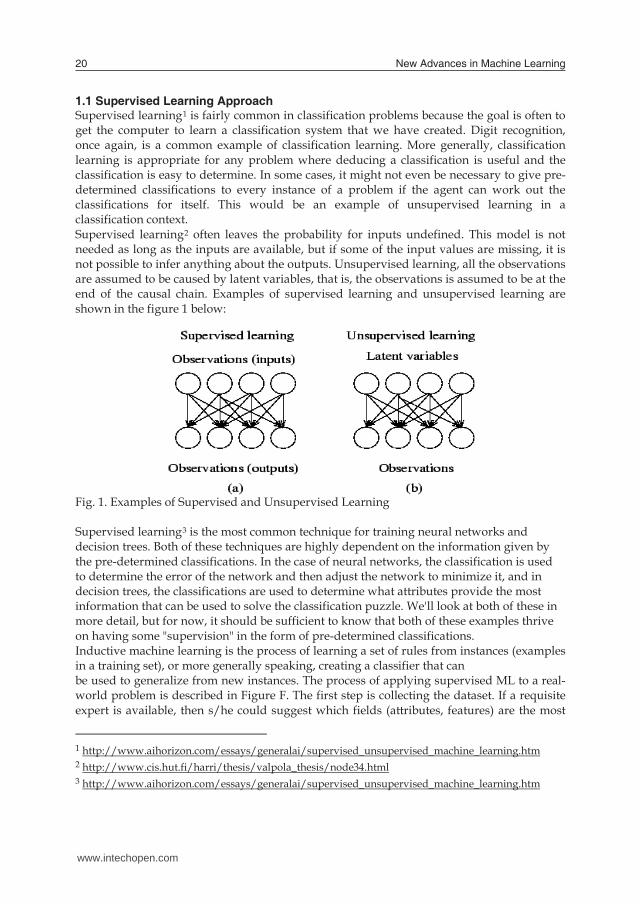
Fig. 1. Examples of Supervised and Unsupervised Learning
often leaves the probability for inputs undefined. This model is not needed as long as the inputs are available, but if some of the input values are missing, it is not possible to infer anything about the outputs. Unsupervised learning, all the observations are assumed to be caused by latent variables, that is, the observations is assumed to be at the end of the causal chain. Examples of supervised learning and unsupervised learning are shown in the figure 1 below:
Supervised learning3
be used to generalize from new instances. The process of applying supervised ML to a real-world problem is described in Figure F. The first step is collecting the dataset. If a requisite expert is available, then s/he could suggest which fields (attributes, features) are the most
is the most common technique for training neural networks and decision trees. Both of these techniques are highly dependent on the information given by the pre-determined classifications. In the case of neural networks, the classification is used to determine the error of the network and then adjust the network to minimize it, and in decision trees, the classifications are used to determine what attributes provide the most information that can be used to solve the classification puzzle. We'll look at both of these in more detail, but for now, it should be sufficient to know that both of these examples thrive on having some "supervision" in the form of pre-determined classifications. Inductive machine learning is the process of learning a set of rules from instances (examples in a training set), or more generally speaking, creating a classifier that can
1 http://www.aihorizon.com/essays/generalai/supervised_unsupervised_machine_learning.htm 2 http://www.cis.hut.fi/harri/thesis/valpola_thesis/node34.html 3 http://www.aihorizon.com/essays/generalai/supervised_unsupervised_machine_learning.htm
informative. If not, then the simplest method is that of “brute-force,” which means measuring everything available in the hope that the right (informative, relevant) features can be isolated. However, a dataset collected by the “brute-force” method is not directly suitable for induction. It contains in most cases noise and missing feature values, and therefore requires significant pre-processing according to Zhang et al (Zhang, 2002). The second step is the data preparation and data pre-processing. Depending on the circumstances, researchers have a number of methods to choose from to handle missing data (Batista, 2003). Hodge et al (Hodge, 2004) , have recently introduced a survey of contemporary techniques for outlier (noise) detection. These researchers have identified the techniques’ advantages and disadvantages. Instance selection is not only used to handle noise but to cope with the infeasibility of learning from very large datasets. Instance selection in these datasets is an optimization problem that attempts to maintain the mining quality while minimizing the sample size. It reduces data and enables a data mining algorithm to function and work effectively with very large datasets. There is a variety of procedures for sampling instances from a large dataset. See figure 2 below. Feature subset selection is the process of identifying and removing as many irrelevant and redundant features as possible (Yu, 2004) . This reduces the dimensionality of the data and enables data mining algorithms to operate faster and more effectively. The fact that many features depend on one another often unduly influences the accuracy of supervised ML classification models. This problem can be addressed by constructing new features from the basic feature set. This technique is called feature construction/transformation. These newly generated features may lead to the creation of more concise and accurate classifiers. In addition, the discovery of meaningful features contributes to better comprehensibility of the produced classifier, and a better understanding of the learned concept.Speech recognition using hidden Markov models and Bayesian networks relies on some elements of supervision as well in order to adjust parameters to, as usual, minimize the error on the given inputs.Notice something important here: in the classification problem, the goal of the learning algorithm is to minimize the error with respect to the given inputs. These inputs, often called the "training set", are the examples from which the agent tries to learn. But learning the training set well is not necessarily the best thing to do. For instance, if I tried to teach you exclusive-or, but only showed you combinations consisting of one true and one false, but never both false or both true, you might learn the rule that the answer is always true. Similarly, with machine learning algorithms, a common problem is over-fitting the data and essentially memorizing the training set rather than learning a more general classification technique. As you might imagine, not all training sets have the inputs classified correctly. This can lead to problems if the algorithm used is powerful enough to memorize even the apparently "special cases" that don't fit the more general principles. This, too, can lead to over fitting, and it is a challenge to find algorithms that are both powerful enough to learn complex functions and robust enough to produce generalisable results.
www.intechopen.com
Types of Machine Learning Algorithms 21
1.1 Supervised Learning Approach Supervised learning1
Supervised learning
is fairly common in classification problems because the goal is often to get the computer to learn a classification system that we have created. Digit recognition, once again, is a common example of classification learning. More generally, classification learning is appropriate for any problem where deducing a classification is useful and the classification is easy to determine. In some cases, it might not even be necessary to give pre-determined classifications to every instance of a problem if the agent can work out the classifications for itself. This would be an example of unsupervised learning in a classification context.
2
Fig. 1. Examples of Supervised and Unsupervised Learning
often leaves the probability for inputs undefined. This model is not needed as long as the inputs are available, but if some of the input values are missing, it is not possible to infer anything about the outputs. Unsupervised learning, all the observations are assumed to be caused by latent variables, that is, the observations is assumed to be at the end of the causal chain. Examples of supervised learning and unsupervised learning are shown in the figure 1 below:
Supervised learning3
be used to generalize from new instances. The process of applying supervised ML to a real-world problem is described in Figure F. The first step is collecting the dataset. If a requisite expert is available, then s/he could suggest which fields (attributes, features) are the most
is the most common technique for training neural networks and decision trees. Both of these techniques are highly dependent on the information given by the pre-determined classifications. In the case of neural networks, the classification is used to determine the error of the network and then adjust the network to minimize it, and in decision trees, the classifications are used to determine what attributes provide the most information that can be used to solve the classification puzzle. We'll look at both of these in more detail, but for now, it should be sufficient to know that both of these examples thrive on having some "supervision" in the form of pre-determined classifications. Inductive machine learning is the process of learning a set of rules from instances (examples in a training set), or more generally speaking, creating a classifier that can
1 http://www.aihorizon.com/essays/generalai/supervised_unsupervised_machine_learning.htm 2 http://www.cis.hut.fi/harri/thesis/valpola_thesis/node34.html 3 http://www.aihorizon.com/essays/generalai/supervised_unsupervised_machine_learning.htm
informative. If not, then the simplest method is that of “brute-force,” which means measuring everything available in the hope that the right (informative, relevant) features can be isolated. However, a dataset collected by the “brute-force” method is not directly suitable for induction. It contains in most cases noise and missing feature values, and therefore requires significant pre-processing according to Zhang et al (Zhang, 2002). The second step is the data preparation and data pre-processing. Depending on the circumstances, researchers have a number of methods to choose from to handle missing data (Batista, 2003). Hodge et al (Hodge, 2004) , have recently introduced a survey of contemporary techniques for outlier (noise) detection. These researchers have identified the techniques’ advantages and disadvantages. Instance selection is not only used to handle noise but to cope with the infeasibility of learning from very large datasets. Instance selection in these datasets is an optimization problem that attempts to maintain the mining quality while minimizing the sample size. It reduces data and enables a data mining algorithm to function and work effectively with very large datasets. There is a variety of procedures for sampling instances from a large dataset. See figure 2 below. Feature subset selection is the process of identifying and removing as many irrelevant and redundant features as possible (Yu, 2004) . This reduces the dimensionality of the data and enables data mining algorithms to operate faster and more effectively. The fact that many features depend on one another often unduly influences the accuracy of supervised ML classification models. This problem can be addressed by constructing new features from the basic feature set. This technique is called feature construction/transformation. These newly generated features may lead to the creation of more concise and accurate classifiers. In addition, the discovery of meaningful features contributes to better comprehensibility of the produced classifier, and a better understanding of the learned concept.Speech recognition using hidden Markov models and Bayesian networks relies on some elements of supervision as well in order to adjust parameters to, as usual, minimize the error on the given inputs.Notice something important here: in the classification problem, the goal of the learning algorithm is to minimize the error with respect to the given inputs. These inputs, often called the "training set", are the examples from which the agent tries to learn. But learning the training set well is not necessarily the best thing to do. For instance, if I tried to teach you exclusive-or, but only showed you combinations consisting of one true and one false, but never both false or both true, you might learn the rule that the answer is always true. Similarly, with machine learning algorithms, a common problem is over-fitting the data and essentially memorizing the training set rather than learning a more general classification technique. As you might imagine, not all training sets have the inputs classified correctly. This can lead to problems if the algorithm used is powerful enough to memorize even the apparently "special cases" that don't fit the more general principles. This, too, can lead to over fitting, and it is a challenge to find algorithms that are both powerful enough to learn complex functions and robust enough to produce generalisable results.
www.intechopen.com
New Advances in Machine Learning22
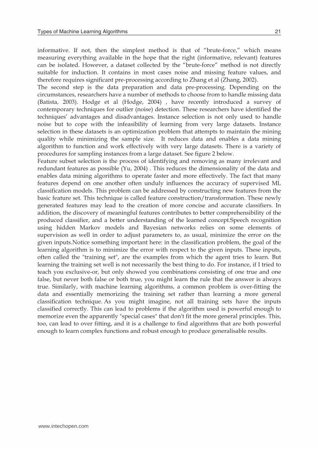
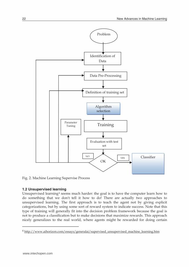
Fig. 2. Machine Learning Supervise Process
1.2 Unsupervised learning Unsupervised learning4
4
seems much harder: the goal is to have the computer learn how to do something that we don't tell it how to do! There are actually two approaches to unsupervised learning. The first approach is to teach the agent not by giving explicit categorizations, but by using some sort of reward system to indicate success. Note that this type of training will generally fit into the decision problem framework because the goal is not to produce a classification but to make decisions that maximize rewards. This approach nicely generalizes to the real world, where agents might be rewarded for doing certain
http://www.aihorizon.com/essays/generalai/supervised_unsupervised_machine_learning.htm
Problem
Identification of Data
Data Pre-Processing
Definition of training set
Algorithm selection
Training
Evaluation with test set
OK Classifier
Parameter Tuning
YES NO
actions and punished for doing others. Often, a form of reinforcement learning can be used for unsupervised learning, where the agent bases its actions on the previous rewards and punishments without necessarily even learning any information about the exact ways that its actions affect the world. In a way, all of this information is unnecessary because by learning a reward function, the agent simply knows what to do without any processing because it knows the exact reward it expects to achieve for each action it could take. This can be extremely beneficial in cases where calculating every possibility is very time consuming (even if all of the transition probabilities between world states were known). On the other hand, it can be very time consuming to learn by, essentially, trial and error. But this kind of learning can be powerful because it assumes no pre-discovered classification of examples. In some cases, for example, our classifications may not be the best possible. One striking exmaple is that the conventional wisdom about the game of backgammon was turned on its head when a series of computer programs (neuro-gammon and TD-gammon) that learned through unsupervised learning became stronger than the best human chess players merely by playing themselves over and over. These programs discovered some principles that surprised the backgammon experts and performed better than backgammon programs trained on pre-classified examples. A second type of unsupervised learning is called clustering. In this type of learning, the goal is not to maximize a utility function, but simply to find similarities in the training data. The assumption is often that the clusters discovered will match reasonably well with an intuitive classification. For instance, clustering individuals based on demographics might result in a clustering of the wealthy in one group and the poor in another. Although the algorithm won't have names to assign to these clusters, it can produce them and then use those clusters to assign new examples into one or the other of the clusters. This is a data-driven approach that can work well when there is sufficient data; for instance, social information filtering algorithms, such as those that Amazon.com use to recommend books, are based on the principle of finding similar groups of people and then assigning new users to groups. In some cases, such as with social information filtering, the information about other members of a cluster (such as what books they read) can be sufficient for the algorithm to produce meaningful results. In other cases, it may be the case that the clusters are merely a useful tool for a human analyst. Unfortunately, even unsupervised learning suffers from the problem of overfitting the training data. There's no silver bullet to avoiding the problem because any algorithm that can learn from its inputs needs to be quite powerful. Unsupervised learning algorithms according to Ghahramani (Ghahramani, 2008) are designed to extract structure from data samples. The quality of a structure is measured by a cost function which is usually minimized to infer optimal parameters characterizing the hidden structure in the data. Reliable and robust inference requires a guarantee that extracted structures are typical for the data source, i.e., similar structures have to be extracted from a second sample set of the same data source. Lack of robustness is known as over fitting from the statistics and the machine learning literature. In this talk I characterize the over fitting phenomenon for a class of histogram clustering models which play a prominent role in information retrieval, linguistic and computer vision applications. Learning algorithms with robustness to sample fluctuations are derived from large deviation results and the maximum entropy principle for the learning process.
www.intechopen.com
Types of Machine Learning Algorithms 23
Fig. 2. Machine Learning Supervise Process
1.2 Unsupervised learning Unsupervised learning4
4
seems much harder: the goal is to have the computer learn how to do something that we don't tell it how to do! There are actually two approaches to unsupervised learning. The first approach is to teach the agent not by giving explicit categorizations, but by using some sort of reward system to indicate success. Note that this type of training will generally fit into the decision problem framework because the goal is not to produce a classification but to make decisions that maximize rewards. This approach nicely generalizes to the real world, where agents might be rewarded for doing certain
http://www.aihorizon.com/essays/generalai/supervised_unsupervised_machine_learning.htm
Problem
Identification of Data
Data Pre-Processing
Definition of training set
Algorithm selection
Training
Evaluation with test set
OK Classifier
Parameter Tuning
YES NO
actions and punished for doing others. Often, a form of reinforcement learning can be used for unsupervised learning, where the agent bases its actions on the previous rewards and punishments without necessarily even learning any information about the exact ways that its actions affect the world. In a way, all of this information is unnecessary because by learning a reward function, the agent simply knows what to do without any processing because it knows the exact reward it expects to achieve for each action it could take. This can be extremely beneficial in cases where calculating every possibility is very time consuming (even if all of the transition probabilities between world states were known). On the other hand, it can be very time consuming to learn by, essentially, trial and error. But this kind of learning can be powerful because it assumes no pre-discovered classification of examples. In some cases, for example, our classifications may not be the best possible. One striking exmaple is that the conventional wisdom about the game of backgammon was turned on its head when a series of computer programs (neuro-gammon and TD-gammon) that learned through unsupervised learning became stronger than the best human chess players merely by playing themselves over and over. These programs discovered some principles that surprised the backgammon experts and performed better than backgammon programs trained on pre-classified examples. A second type of unsupervised learning is called clustering. In this type of learning, the goal is not to maximize a utility function, but simply to find similarities in the training data. The assumption is often that the clusters discovered will match reasonably well with an intuitive classification. For instance, clustering individuals based on demographics might result in a clustering of the wealthy in one group and the poor in another. Although the algorithm won't have names to assign to these clusters, it can produce them and then use those clusters to assign new examples into one or the other of the clusters. This is a data-driven approach that can work well when there is sufficient data; for instance, social information filtering algorithms, such as those that Amazon.com use to recommend books, are based on the principle of finding similar groups of people and then assigning new users to groups. In some cases, such as with social information filtering, the information about other members of a cluster (such as what books they read) can be sufficient for the algorithm to produce meaningful results. In other cases, it may be the case that the clusters are merely a useful tool for a human analyst. Unfortunately, even unsupervised learning suffers from the problem of overfitting the training data. There's no silver bullet to avoiding the problem because any algorithm that can learn from its inputs needs to be quite powerful. Unsupervised learning algorithms according to Ghahramani (Ghahramani, 2008) are designed to extract structure from data samples. The quality of a structure is measured by a cost function which is usually minimized to infer optimal parameters characterizing the hidden structure in the data. Reliable and robust inference requires a guarantee that extracted structures are typical for the data source, i.e., similar structures have to be extracted from a second sample set of the same data source. Lack of robustness is known as over fitting from the statistics and the machine learning literature. In this talk I characterize the over fitting phenomenon for a class of histogram clustering models which play a prominent role in information retrieval, linguistic and computer vision applications. Learning algorithms with robustness to sample fluctuations are derived from large deviation results and the maximum entropy principle for the learning process.
www.intechopen.com
New Advances in Machine Learning24
Unsupervised learning has produced many successes, such as world-champion calibre backgammon programs and even machines capable of driving cars! It can be a powerful technique when there is an easy way to assign values to actions. Clustering can be useful when there is enough data to form clusters (though this turns out to be difficult at times) and especially when additional data about members of a cluster can be used to produce further results due to dependencies in the data. Classification learning is powerful when the classifications are known to be correct (for instance, when dealing with diseases, it's generally straight-forward to determine the design after the fact by an autopsy), or when the classifications are simply arbitrary things that we would like the computer to be able to recognize for us. Classification learning is often necessary when the decisions made by the algorithm will be required as input somewhere else. Otherwise, it wouldn't be easy for whoever requires that input to figure out what it means. Both techniques can be valuable and which one you choose should depend on the circumstances--what kind of problem is being solved, how much time is allotted to solving it (supervised learning or clustering is often faster than reinforcement learning techniques), and whether supervised learning is even possible.
1.3 Algorithm Types In the area of supervised learning which deals much with classification. These are the algorithms types:
• Linear Classifiers Logical Regression Naïve Bayes Classifier Perceptron Support Vector Machine
• Quadratic Classifiers • K-Means Clustering • Boosting • Decision Tree
Random Forest • Neural networks • Bayesian Networks
Linear Classifiers: In machine learning, the goal of classification is to group items that have similar feature values, into groups. Timothy et al (Timothy Jason Shepard, 1998) stated that a linear classifier achieves this by making a classification decision based on the value of the linear combination of the features. If the input feature vector to the classifier is a real vector , then the output score is
where is a real vector of weights and f is a function that converts the dot product of the two vectors into the desired output. The weight vector is learned from a set of labelled training samples. Often f is a simple function that maps all values above a certain threshold to the first class and all other values to the second class. A more complex f might give the probability that an item belongs to a certain class. For a two-class classification problem, one can visualize the operation of a linear classifier as splitting a high-dimensional input space with a hyperplane: all points on one side of the hyper plane are classified as "yes", while the others are classified as "no". A linear classifier is often used in situations where the speed of classification is an issue, since it is often the fastest classifier, especially when is sparse. However, decision trees can be faster. Also, linear classifiers often work very well when the number of dimensions in is large, as in document classification, where each element in is typically the number of counts of a word in a document (see document-term matrix). In such cases, the classifier should be well-regularized.
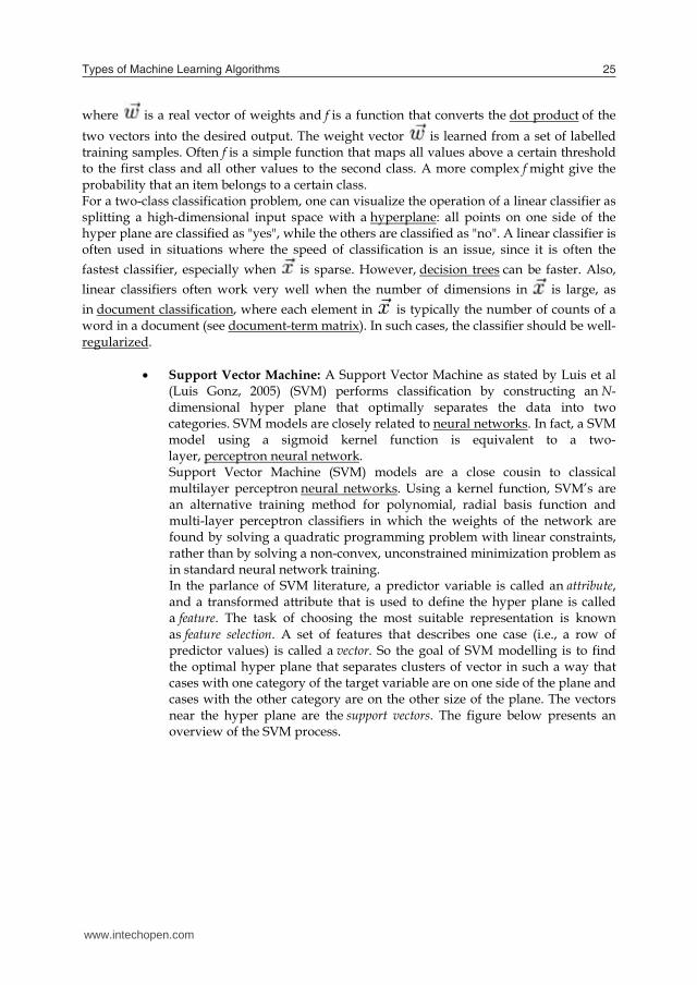
• Support Vector Machine: A Support Vector Machine as stated by Luis et al (Luis Gonz, 2005) (SVM) performs classification by constructing an N-dimensional hyper plane that optimally separates the data into two categories. SVM models are closely related to neural networks. In fact, a SVM model using a sigmoid kernel function is equivalent to a two-layer, perceptron neural network. Support Vector Machine (SVM) models are a close cousin to classical multilayer perceptron neural networks. Using a kernel function, SVM’s are an alternative training method for polynomial, radial basis function and multi-layer perceptron classifiers in which the weights of the network are found by solving a quadratic programming problem with linear constraints, rather than by solving a non-convex, unconstrained minimization problem as in standard neural network training. In the parlance of SVM literature, a predictor variable is called an attribute, and a transformed attribute that is used to define the hyper plane is called a feature. The task of choosing the most suitable representation is known as feature selection. A set of features that describes one case (i.e., a row of predictor values) is called a vector. So the goal of SVM modelling is to find the optimal hyper plane that separates clusters of vector in such a way that cases with one category of the target variable are on one side of the plane and cases with the other category are on the other size of the plane. The vectors near the hyper plane are the support vectors. The figure below presents an overview of the SVM process.
www.intechopen.com
Types of Machine Learning Algorithms 25
Unsupervised learning has produced many successes, such as world-champion calibre backgammon programs and even machines capable of driving cars! It can be a powerful technique when there is an easy way to assign values to actions. Clustering can be useful when there is enough data to form clusters (though this turns out to be difficult at times) and especially when additional data about members of a cluster can be used to produce further results due to dependencies in the data. Classification learning is powerful when the classifications are known to be correct (for instance, when dealing with diseases, it's generally straight-forward to determine the design after the fact by an autopsy), or when the classifications are simply arbitrary things that we would like the computer to be able to recognize for us. Classification learning is often necessary when the decisions made by the algorithm will be required as input somewhere else. Otherwise, it wouldn't be easy for whoever requires that input to figure out what it means. Both techniques can be valuable and which one you choose should depend on the circumstances--what kind of problem is being solved, how much time is allotted to solving it (supervised learning or clustering is often faster than reinforcement learning techniques), and whether supervised learning is even possible.
1.3 Algorithm Types In the area of supervised learning which deals much with classification. These are the algorithms types:
• Linear Classifiers Logical Regression Naïve Bayes Classifier Perceptron Support Vector Machine
• Quadratic Classifiers • K-Means Clustering • Boosting • Decision Tree
Random Forest • Neural networks • Bayesian Networks
Linear Classifiers: In machine learning, the goal of classification is to group items that have similar feature values, into groups. Timothy et al (Timothy Jason Shepard, 1998) stated that a linear classifier achieves this by making a classification decision based on the value of the linear combination of the features. If the input feature vector to the classifier is a real vector , then the output score is
where is a real vector of weights and f is a function that converts the dot product of the two vectors into the desired output. The weight vector is learned from a set of labelled training samples. Often f is a simple function that maps all values above a certain threshold to the first class and all other values to the second class. A more complex f might give the probability that an item belongs to a certain class. For a two-class classification problem, one can visualize the operation of a linear classifier as splitting a high-dimensional input space with a hyperplane: all points on one side of the hyper plane are classified as "yes", while the others are classified as "no". A linear classifier is often used in situations where the speed of classification is an issue, since it is often the fastest classifier, especially when is sparse. However, decision trees can be faster. Also, linear classifiers often work very well when the number of dimensions in is large, as in document classification, where each element in is typically the number of counts of a word in a document (see document-term matrix). In such cases, the classifier should be well-regularized.
• Support Vector Machine: A Support Vector Machine as stated by Luis et al (Luis Gonz, 2005) (SVM) performs classification by constructing an N-dimensional hyper plane that optimally separates the data into two categories. SVM models are closely related to neural networks. In fact, a SVM model using a sigmoid kernel function is equivalent to a two-layer, perceptron neural network. Support Vector Machine (SVM) models are a close cousin to classical multilayer perceptron neural networks. Using a kernel function, SVM’s are an alternative training method for polynomial, radial basis function and multi-layer perceptron classifiers in which the weights of the network are found by solving a quadratic programming problem with linear constraints, rather than by solving a non-convex, unconstrained minimization problem as in standard neural network training. In the parlance of SVM literature, a predictor variable is called an attribute, and a transformed attribute that is used to define the hyper plane is called a feature. The task of choosing the most suitable representation is known as feature selection. A set of features that describes one case (i.e., a row of predictor values) is called a vector. So the goal of SVM modelling is to find the optimal hyper plane that separates clusters of vector in such a way that cases with one category of the target variable are on one side of the plane and cases with the other category are on the other size of the plane. The vectors near the hyper plane are the support vectors. The figure below presents an overview of the SVM process.
www.intechopen.com
New Advances in Machine Learning26
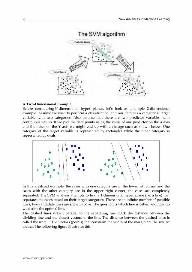
A Two-Dimensional Example Before considering N-dimensional hyper planes, let’s look at a simple 2-dimensional example. Assume we wish to perform a classification, and our data has a categorical target variable with two categories. Also assume that there are two predictor variables with continuous values. If we plot the data points using the value of one predictor on the X axis and the other on the Y axis we might end up with an image such as shown below. One category of the target variable is represented by rectangles while the other category is represented by ovals.
In this idealized example, the cases with one category are in the lower left corner and the cases with the other category are in the upper right corner; the cases are completely separated. The SVM analysis attempts to find a 1-dimensional hyper plane (i.e. a line) that separates the cases based on their target categories. There are an infinite number of possible lines; two candidate lines are shown above. The question is which line is better, and how do we define the optimal line. The dashed lines drawn parallel to the separating line mark the distance between the dividing line and the closest vectors to the line. The distance between the dashed lines is called the margin. The vectors (points) that constrain the width of the margin are the support vectors. The following figure illustrates this.
An SVM analysis (Luis Gonz, 2005) finds the line (or, in general, hyper plane) that is oriented so that the margin between the support vectors is maximized. In the figure above, the line in the right panel is superior to the line in the left panel. If all analyses consisted of two-category target variables with two predictor variables, and the cluster of points could be divided by a straight line, life would be easy. Unfortunately, this is not generally the case, so SVM must deal with (a) more than two predictor variables, (b) separating the points with non-linear curves, (c) handling the cases where clusters cannot be completely separated, and (d) handling classifications with more than two categories. In this chapter, we shall explain three main machine learning techniques with their examples and how they perform in reality. These are:
• K-Means Clustering • Neural Network • Self Organised Map
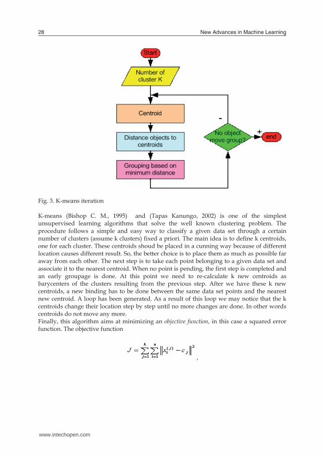
1.3.1 K-Means Clustering The basic step of k-means clustering is uncomplicated. In the beginning we determine number of cluster K and we assume the centre of these clusters. We can take any random objects as the initial centre or the first K objects in sequence can also serve as the initial centre. Then the K means algorithm will do the three steps below until convergence. Iterate until stable (= no object move group):
1. Determine the centre coordinate
2. Determine the distance of each object to the centre
3. Group the object based on minimum distance
The Figure 3 shows a K- means flow diagram
www.intechopen.com

Types of Machine Learning Algorithms 27
A Two-Dimensional Example Before considering N-dimensional hyper planes, let’s look at a simple 2-dimensional example. Assume we wish to perform a classification, and our data has a categorical target variable with two categories. Also assume that there are two predictor variables with continuous values. If we plot the data points using the value of one predictor on the X axis and the other on the Y axis we might end up with an image such as shown below. One category of the target variable is represented by rectangles while the other category is represented by ovals.
In this idealized example, the cases with one category are in the lower left corner and the cases with the other category are in the upper right corner; the cases are completely separated. The SVM analysis attempts to find a 1-dimensional hyper plane (i.e. a line) that separates the cases based on their target categories. There are an infinite number of possible lines; two candidate lines are shown above. The question is which line is better, and how do we define the optimal line. The dashed lines drawn parallel to the separating line mark the distance between the dividing line and the closest vectors to the line. The distance between the dashed lines is called the margin. The vectors (points) that constrain the width of the margin are the support vectors. The following figure illustrates this.
An SVM analysis (Luis Gonz, 2005) finds the line (or, in general, hyper plane) that is oriented so that the margin between the support vectors is maximized. In the figure above, the line in the right panel is superior to the line in the left panel. If all analyses consisted of two-category target variables with two predictor variables, and the cluster of points could be divided by a straight line, life would be easy. Unfortunately, this is not generally the case, so SVM must deal with (a) more than two predictor variables, (b) separating the points with non-linear curves, (c) handling the cases where clusters cannot be completely separated, and (d) handling classifications with more than two categories. In this chapter, we shall explain three main machine learning techniques with their examples and how they perform in reality. These are:
• K-Means Clustering • Neural Network • Self Organised Map
1.3.1 K-Means Clustering The basic step of k-means clustering is uncomplicated. In the beginning we determine number of cluster K and we assume the centre of these clusters. We can take any random objects as the initial centre or the first K objects in sequence can also serve as the initial centre. Then the K means algorithm will do the three steps below until convergence. Iterate until stable (= no object move group):
1. Determine the centre coordinate
2. Determine the distance of each object to the centre
3. Group the object based on minimum distance
The Figure 3 shows a K- means flow diagram
www.intechopen.com
New Advances in Machine Learning28
Fig. 3. K-means iteration K-means (Bishop C. M., 1995) and (Tapas Kanungo, 2002) is one of the simplest unsupervised learning algorithms that solve the well known clustering problem. The procedure follows a simple and easy way to classify a given data set through a certain number of clusters (assume k clusters) fixed a priori. The main idea is to define k centroids, one for each cluster. These centroids shoud be placed in a cunning way because of different location causes different result. So, the better choice is to place them as much as possible far away from each other. The next step is to take each point belonging to a given data set and associate it to the nearest centroid. When no point is pending, the first step is completed and an early groupage is done. At this point we need to re-calculate k new centroids as barycenters of the clusters resulting from the previous step. After we have these k new centroids, a new binding has to be done between the same data set points and the nearest new centroid. A loop has been generated. As a result of this loop we may notice that the k centroids change their location step by step until no more changes are done. In other words centroids do not move any more. Finally, this algorithm aims at minimizing an objective function, in this case a squared error function. The objective function
,
where is a chosen distance measure between a data point and the cluster
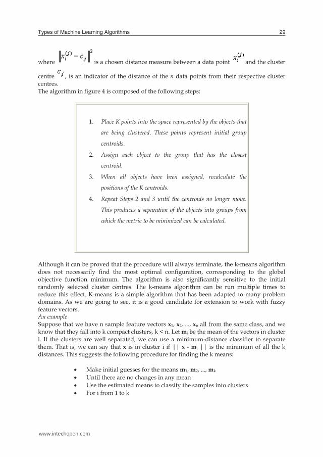
centre , is an indicator of the distance of the n data points from their respective cluster centres. The algorithm in figure 4 is composed of the following steps:
1. Place K points into the space represented by the objects that
are being clustered. These points represent initial group
centroids.
2. Assign each object to the group that has the closest
centroid.
3. When all objects have been assigned, recalculate the
positions of the K centroids.
4. Repeat Steps 2 and 3 until the centroids no longer move.
This produces a separation of the objects into groups from
which the metric to be minimized can be calculated.
Although it can be proved that the procedure will always terminate, the k-means algorithm does not necessarily find the most optimal configuration, corresponding to the global objective function minimum. The algorithm is also significantly sensitive to the initial randomly selected cluster centres. The k-means algorithm can be run multiple times to reduce this effect. K-means is a simple algorithm that has been adapted to many problem domains. As we are going to see, it is a good candidate for extension to work with fuzzy feature vectors. An example Suppose that we have n sample feature vectors x1, x2, ..., xn all from the same class, and we know that they fall into k compact clusters, k < n. Let mi be the mean of the vectors in cluster i. If the clusters are well separated, we can use a minimum-distance classifier to separate them. That is, we can say that x is in cluster i if || x - mi || is the minimum of all the k distances. This suggests the following procedure for finding the k means:
• Make initial guesses for the means m1, m2, ..., mk • Until there are no changes in any mean • Use the estimated means to classify the samples into clusters • For i from 1 to k
www.intechopen.com
Types of Machine Learning Algorithms 29
Fig. 3. K-means iteration K-means (Bishop C. M., 1995) and (Tapas Kanungo, 2002) is one of the simplest unsupervised learning algorithms that solve the well known clustering problem. The procedure follows a simple and easy way to classify a given data set through a certain number of clusters (assume k clusters) fixed a priori. The main idea is to define k centroids, one for each cluster. These centroids shoud be placed in a cunning way because of different location causes different result. So, the better choice is to place them as much as possible far away from each other. The next step is to take each point belonging to a given data set and associate it to the nearest centroid. When no point is pending, the first step is completed and an early groupage is done. At this point we need to re-calculate k new centroids as barycenters of the clusters resulting from the previous step. After we have these k new centroids, a new binding has to be done between the same data set points and the nearest new centroid. A loop has been generated. As a result of this loop we may notice that the k centroids change their location step by step until no more changes are done. In other words centroids do not move any more. Finally, this algorithm aims at minimizing an objective function, in this case a squared error function. The objective function
,
where is a chosen distance measure between a data point and the cluster
centre , is an indicator of the distance of the n data points from their respective cluster centres. The algorithm in figure 4 is composed of the following steps:
1. Place K points into the space represented by the objects that
are being clustered. These points represent initial group
centroids.
2. Assign each object to the group that has the closest
centroid.
3. When all objects have been assigned, recalculate the
positions of the K centroids.
4. Repeat Steps 2 and 3 until the centroids no longer move.
This produces a separation of the objects into groups from
which the metric to be minimized can be calculated.
Although it can be proved that the procedure will always terminate, the k-means algorithm does not necessarily find the most optimal configuration, corresponding to the global objective function minimum. The algorithm is also significantly sensitive to the initial randomly selected cluster centres. The k-means algorithm can be run multiple times to reduce this effect. K-means is a simple algorithm that has been adapted to many problem domains. As we are going to see, it is a good candidate for extension to work with fuzzy feature vectors. An example Suppose that we have n sample feature vectors x1, x2, ..., xn all from the same class, and we know that they fall into k compact clusters, k < n. Let mi be the mean of the vectors in cluster i. If the clusters are well separated, we can use a minimum-distance classifier to separate them. That is, we can say that x is in cluster i if || x - mi || is the minimum of all the k distances. This suggests the following procedure for finding the k means:
• Make initial guesses for the means m1, m2, ..., mk • Until there are no changes in any mean • Use the estimated means to classify the samples into clusters • For i from 1 to k
www.intechopen.com
New Advances in Machine Learning30
• Replace mi with the mean of all of the samples for cluster i
• end_for • end_until
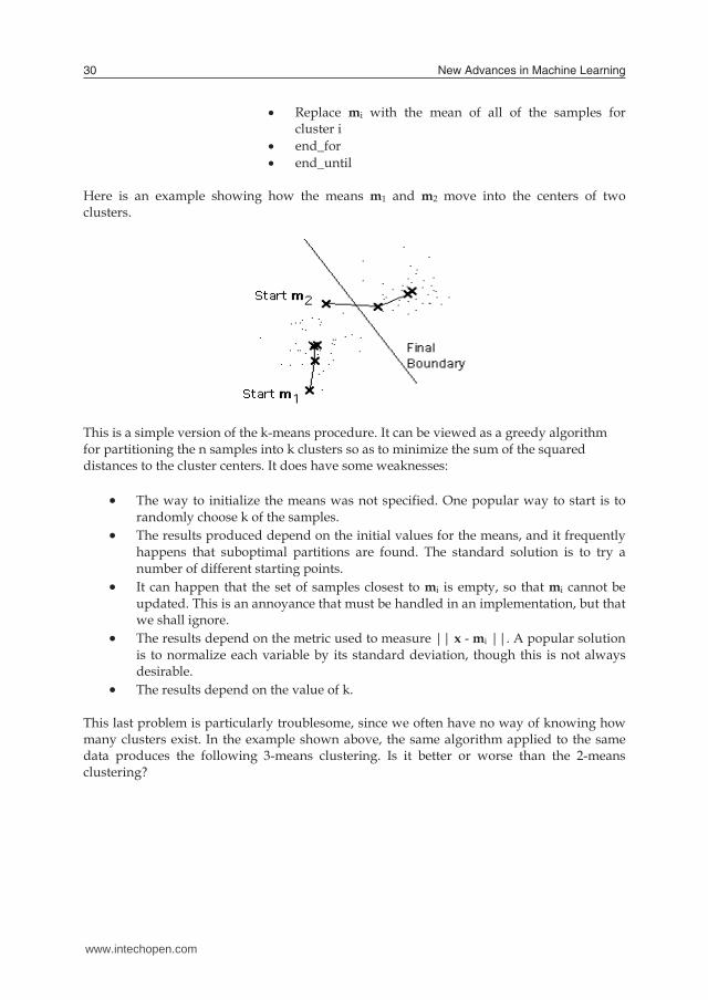
Here is an example showing how the means m1 and m2 move into the centers of two clusters.
This is a simple version of the k-means procedure. It can be viewed as a greedy algorithm for partitioning the n samples into k clusters so as to minimize the sum of the squared distances to the cluster centers. It does have some weaknesses: • The way to initialize the means was not specified. One popular way to start is to
randomly choose k of the samples. • The results produced depend on the initial values for the means, and it frequently happens that suboptimal partitions are found. The standard solution is to try a number of different starting points. • It can happen that the set of samples closest to mi is empty, so that mi cannot be updated. This is an annoyance that must be handled in an implementation, but that we shall ignore. • The results depend on the metric used to measure || x - mi ||. A popular solution is to normalize each variable by its standard deviation, though this is not always desirable. • The results depend on the value of k.
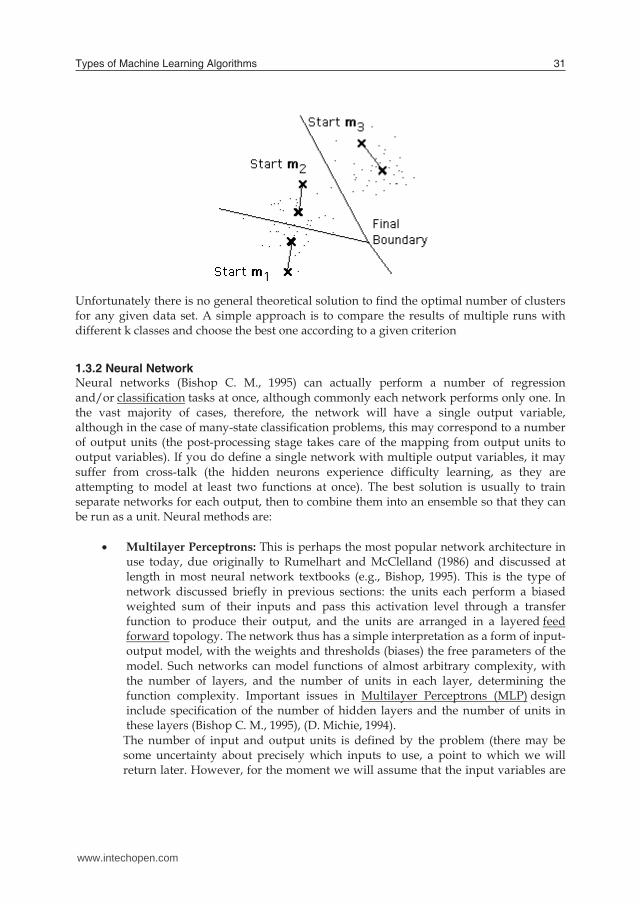
This last problem is particularly troublesome, since we often have no way of knowing how many clusters exist. In the example shown above, the same algorithm applied to the same data produces the following 3-means clustering. Is it better or worse than the 2-means clustering?
Unfortunately there is no general theoretical solution to find the optimal number of clusters for any given data set. A simple approach is to compare the results of multiple runs with different k classes and choose the best one according to a given criterion
1.3.2 Neural Network Neural networks (Bishop C. M., 1995) can actually perform a number of regression and/or classification tasks at once, although commonly each network performs only one. In the vast majority of cases, therefore, the network will have a single output variable, although in the case of many-state classification problems, this may correspond to a number of output units (the post-processing stage takes care of the mapping from output units to output variables). If you do define a single network with multiple output variables, it may suffer from cross-talk (the hidden neurons experience difficulty learning, as they are attempting to model at least two functions at once). The best solution is usually to train separate networks for each output, then to combine them into an ensemble so that they can be run as a unit. Neural methods are:
• Multilayer Perceptrons: This is perhaps the most popular network architecture in use today, due originally to Rumelhart and McClelland (1986) and discussed at length in most neural network textbooks (e.g., Bishop, 1995). This is the type of network discussed briefly in previous sections: the units each perform a biased weighted sum of their inputs and pass this activation level through a transfer function to produce their output, and the units are arranged in a layered feed forward topology. The network thus has a simple interpretation as a form of input-output model, with the weights and thresholds (biases) the free parameters of the model. Such networks can model functions of almost arbitrary complexity, with the number of layers, and the number of units in each layer, determining the function complexity. Important issues in Multilayer Perceptrons (MLP) design include specification of the number of hidden layers and the number of units in these layers (Bishop C. M., 1995), (D. Michie, 1994).
The number of input and output units is defined by the problem (there may be some uncertainty about precisely which inputs to use, a point to which we will return later. However, for the moment we will assume that the input variables are
www.intechopen.com
Types of Machine Learning Algorithms 31
• Replace mi with the mean of all of the samples for cluster i
• end_for • end_until
Here is an example showing how the means m1 and m2 move into the centers of two clusters.
This is a simple version of the k-means procedure. It can be viewed as a greedy algorithm for partitioning the n samples into k clusters so as to minimize the sum of the squared distances to the cluster centers. It does have some weaknesses: • The way to initialize the means was not specified. One popular way to start is to
randomly choose k of the samples. • The results produced depend on the initial values for the means, and it frequently happens that suboptimal partitions are found. The standard solution is to try a number of different starting points. • It can happen that the set of samples closest to mi is empty, so that mi cannot be updated. This is an annoyance that must be handled in an implementation, but that we shall ignore. • The results depend on the metric used to measure || x - mi ||. A popular solution is to normalize each variable by its standard deviation, though this is not always desirable. • The results depend on the value of k.
This last problem is particularly troublesome, since we often have no way of knowing how many clusters exist. In the example shown above, the same algorithm applied to the same data produces the following 3-means clustering. Is it better or worse than the 2-means clustering?
Unfortunately there is no general theoretical solution to find the optimal number of clusters for any given data set. A simple approach is to compare the results of multiple runs with different k classes and choose the best one according to a given criterion
1.3.2 Neural Network Neural networks (Bishop C. M., 1995) can actually perform a number of regression and/or classification tasks at once, although commonly each network performs only one. In the vast majority of cases, therefore, the network will have a single output variable, although in the case of many-state classification problems, this may correspond to a number of output units (the post-processing stage takes care of the mapping from output units to output variables). If you do define a single network with multiple output variables, it may suffer from cross-talk (the hidden neurons experience difficulty learning, as they are attempting to model at least two functions at once). The best solution is usually to train separate networks for each output, then to combine them into an ensemble so that they can be run as a unit. Neural methods are:
• Multilayer Perceptrons: This is perhaps the most popular network architecture in use today, due originally to Rumelhart and McClelland (1986) and discussed at length in most neural network textbooks (e.g., Bishop, 1995). This is the type of network discussed briefly in previous sections: the units each perform a biased weighted sum of their inputs and pass this activation level through a transfer function to produce their output, and the units are arranged in a layered feed forward topology. The network thus has a simple interpretation as a form of input-output model, with the weights and thresholds (biases) the free parameters of the model. Such networks can model functions of almost arbitrary complexity, with the number of layers, and the number of units in each layer, determining the function complexity. Important issues in Multilayer Perceptrons (MLP) design include specification of the number of hidden layers and the number of units in these layers (Bishop C. M., 1995), (D. Michie, 1994).
The number of input and output units is defined by the problem (there may be some uncertainty about precisely which inputs to use, a point to which we will return later. However, for the moment we will assume that the input variables are
www.intechopen.com
New Advances in Machine Learning32
intuitively selected and are all meaningful). The number of hidden units to use is far from clear. As good a starting point as any is to use one hidden layer, with the number of units equal to half the sum of the number of input and output units. Again, we will discuss how to choose a sensible number later.
• Training Multilayer Perceptrons: Once the number of layers, and number of units in each layer, has been selected, the network's weights and thresholds must be set so as to minimize the prediction error made by the network. This is the role of the training algorithms. The historical cases that you have gathered are used to automatically adjust the weights and thresholds in order to minimize this error. This process is equivalent to fitting the model represented by the network to the training data available. The error of a particular configuration of the network can be determined by running all the training cases through the network, comparing the actual output generated with the desired or target outputs. The differences are combined together by an error function to give the network error. The most common error functions are the sum squared error (used for regression problems), where the individual errors of output units on each case are squared and summed together, and the cross entropy functions (used for maximum likelihood classification).
In traditional modeling approaches (e.g., linear modeling) it is possible to algorithmically determine the model configuration that absolutely minimizes this error. The price paid for the greater (non-linear) modeling power of neural networks is that although we can adjust a network to lower its error, we can never be sure that the error could not be lower still.
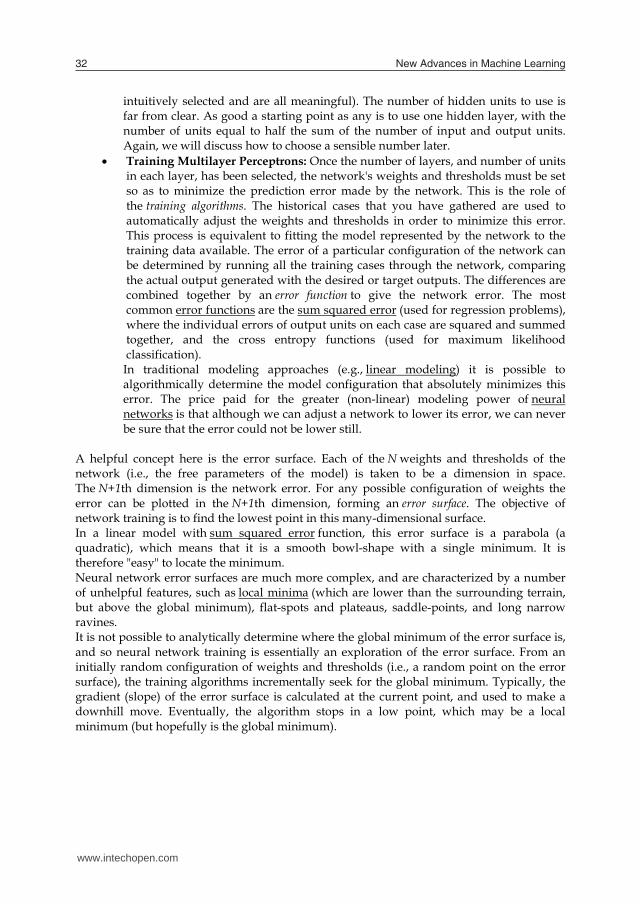
A helpful concept here is the error surface. Each of the N weights and thresholds of the network (i.e., the free parameters of the model) is taken to be a dimension in space. The N+1th dimension is the network error. For any possible configuration of weights the error can be plotted in the N+1th dimension, forming an error surface. The objective of network training is to find the lowest point in this many-dimensional surface. In a linear model with sum squared error function, this error surface is a parabola (a quadratic), which means that it is a smooth bowl-shape with a single minimum. It is therefore "easy" to locate the minimum. Neural network error surfaces are much more complex, and are characterized by a number of unhelpful features, such as local minima (which are lower than the surrounding terrain, but above the global minimum), flat-spots and plateaus, saddle-points, and long narrow ravines. It is not possible to analytically determine where the global minimum of the error surface is, and so neural network training is essentially an exploration of the error surface. From an initially random configuration of weights and thresholds (i.e., a random point on the error surface), the training algorithms incrementally seek for the global minimum. Typically, the gradient (slope) of the error surface is calculated at the current point, and used to make a downhill move. Eventually, the algorithm stops in a low point, which may be a local minimum (but hopefully is the global minimum).
• The Back Propagation Algorithm: The best-known example of a neural network training algorithm is back propagation (Haykin, 19994), (Patterson, 19996), (Fausett, 19994). Modern second-order algorithms such as conjugate gradient descent and Levenberg-Marquardt (see Bishop, 1995; Shepherd, 1997) (both included in ST Neural Networks) are substantially faster (e.g., an order of magnitude faster) for many problems, but back propagation still has advantages in some circumstances, and is the easiest algorithm to understand. We will introduce this now, and discuss the more advanced algorithms later. In back propagation, the gradient vector of the error surface is calculated. This vector points along the line of steepest descent from the current point, so we know that if we move along it a "short" distance, we will decrease the error. A sequence of such moves (slowing as we near the bottom) will eventually find a minimum of some sort. The difficult part is to decide how large the steps should be.
Large steps may converge more quickly, but may also overstep the solution or (if the error surface is very eccentric) go off in the wrong direction. A classic example of this in neural network training is where the algorithm progresses very slowly along a steep, narrow, valley, bouncing from one side across to the other. In contrast, very small steps may go in the correct direction, but they also require a large number of iterations. In practice, the step size is proportional to the slope (so that the algorithm settles down in a minimum) and to a special constant: the learning rate. The correct setting for the learning rate is application-dependent, and is typically chosen by experiment; it may also be time-varying, getting smaller as the algorithm progresses.
The algorithm is also usually modified by inclusion of a momentum term: this encourages movement in a fixed direction, so that if several steps are taken in the same direction, the algorithm "picks up speed", which gives it the ability to (sometimes) escape local minimum, and also to move rapidly over flat spots and plateaus. The algorithm therefore progresses iteratively, through a number of epochs. On each epoch, the training cases are each submitted in turn to the network, and target and actual outputs compared and the error calculated. This error, together with the error surface gradient, is used to adjust the weights, and then the process repeats. The initial network configuration is random, and training stops when a given number of epochs elapses, or when the error reaches an acceptable level, or when the error stops improving (you can select which of these stopping conditions to use).
• Over-learning and Generalization: One major problem with the approach outlined above is that it doesn't actually minimize the error that we are really interested in - which is the expected error the network will make when new cases are submitted to it. In other words, the most desirable property of a network is its ability to generalize to new cases. In reality, the network is trained to minimize the error on the training set, and short of having a perfect and infinitely large training set, this is not the same thing as minimizing the error on the real error surface - the error surface of the underlying and unknown model (Bishop C. M., 1995).
www.intechopen.com
Types of Machine Learning Algorithms 33
intuitively selected and are all meaningful). The number of hidden units to use is far from clear. As good a starting point as any is to use one hidden layer, with the number of units equal to half the sum of the number of input and output units. Again, we will discuss how to choose a sensible number later.
• Training Multilayer Perceptrons: Once the number of layers, and number of units in each layer, has been selected, the network's weights and thresholds must be set so as to minimize the prediction error made by the network. This is the role of the training algorithms. The historical cases that you have gathered are used to automatically adjust the weights and thresholds in order to minimize this error. This process is equivalent to fitting the model represented by the network to the training data available. The error of a particular configuration of the network can be determined by running all the training cases through the network, comparing the actual output generated with the desired or target outputs. The differences are combined together by an error function to give the network error. The most common error functions are the sum squared error (used for regression problems), where the individual errors of output units on each case are squared and summed together, and the cross entropy functions (used for maximum likelihood classification).
In traditional modeling approaches (e.g., linear modeling) it is possible to algorithmically determine the model configuration that absolutely minimizes this error. The price paid for the greater (non-linear) modeling power of neural networks is that although we can adjust a network to lower its error, we can never be sure that the error could not be lower still.
A helpful concept here is the error surface. Each of the N weights and thresholds of the network (i.e., the free parameters of the model) is taken to be a dimension in space. The N+1th dimension is the network error. For any possible configuration of weights the error can be plotted in the N+1th dimension, forming an error surface. The objective of network training is to find the lowest point in this many-dimensional surface. In a linear model with sum squared error function, this error surface is a parabola (a quadratic), which means that it is a smooth bowl-shape with a single minimum. It is therefore "easy" to locate the minimum. Neural network error surfaces are much more complex, and are characterized by a number of unhelpful features, such as local minima (which are lower than the surrounding terrain, but above the global minimum), flat-spots and plateaus, saddle-points, and long narrow ravines. It is not possible to analytically determine where the global minimum of the error surface is, and so neural network training is essentially an exploration of the error surface. From an initially random configuration of weights and thresholds (i.e., a random point on the error surface), the training algorithms incrementally seek for the global minimum. Typically, the gradient (slope) of the error surface is calculated at the current point, and used to make a downhill move. Eventually, the algorithm stops in a low point, which may be a local minimum (but hopefully is the global minimum).
• The Back Propagation Algorithm: The best-known example of a neural network training algorithm is back propagation (Haykin, 19994), (Patterson, 19996), (Fausett, 19994). Modern second-order algorithms such as conjugate gradient descent and Levenberg-Marquardt (see Bishop, 1995; Shepherd, 1997) (both included in ST Neural Networks) are substantially faster (e.g., an order of magnitude faster) for many problems, but back propagation still has advantages in some circumstances, and is the easiest algorithm to understand. We will introduce this now, and discuss the more advanced algorithms later. In back propagation, the gradient vector of the error surface is calculated. This vector points along the line of steepest descent from the current point, so we know that if we move along it a "short" distance, we will decrease the error. A sequence of such moves (slowing as we near the bottom) will eventually find a minimum of some sort. The difficult part is to decide how large the steps should be.
Large steps may converge more quickly, but may also overstep the solution or (if the error surface is very eccentric) go off in the wrong direction. A classic example of this in neural network training is where the algorithm progresses very slowly along a steep, narrow, valley, bouncing from one side across to the other. In contrast, very small steps may go in the correct direction, but they also require a large number of iterations. In practice, the step size is proportional to the slope (so that the algorithm settles down in a minimum) and to a special constant: the learning rate. The correct setting for the learning rate is application-dependent, and is typically chosen by experiment; it may also be time-varying, getting smaller as the algorithm progresses.
The algorithm is also usually modified by inclusion of a momentum term: this encourages movement in a fixed direction, so that if several steps are taken in the same direction, the algorithm "picks up speed", which gives it the ability to (sometimes) escape local minimum, and also to move rapidly over flat spots and plateaus. The algorithm therefore progresses iteratively, through a number of epochs. On each epoch, the training cases are each submitted in turn to the network, and target and actual outputs compared and the error calculated. This error, together with the error surface gradient, is used to adjust the weights, and then the process repeats. The initial network configuration is random, and training stops when a given number of epochs elapses, or when the error reaches an acceptable level, or when the error stops improving (you can select which of these stopping conditions to use).
• Over-learning and Generalization: One major problem with the approach outlined above is that it doesn't actually minimize the error that we are really interested in - which is the expected error the network will make when new cases are submitted to it. In other words, the most desirable property of a network is its ability to generalize to new cases. In reality, the network is trained to minimize the error on the training set, and short of having a perfect and infinitely large training set, this is not the same thing as minimizing the error on the real error surface - the error surface of the underlying and unknown model (Bishop C. M., 1995).
www.intechopen.com
New Advances in Machine Learning34
The most important manifestation of this distinction is the problem of over-learning, or over-fitting. It is easiest to demonstrate this concept using polynomial curve fitting rather than neural networks, but the concept is precisely the same. A polynomial is an equation with terms containing only constants and powers of the variables. For example:
y=2x+3 y=3x2+4x+1
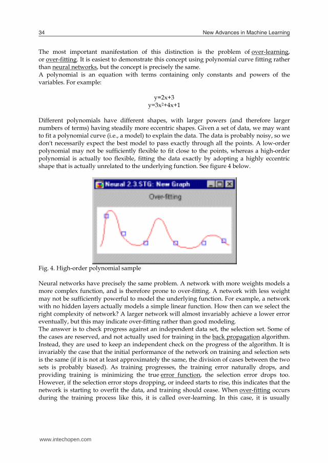
Different polynomials have different shapes, with larger powers (and therefore larger numbers of terms) having steadily more eccentric shapes. Given a set of data, we may want to fit a polynomial curve (i.e., a model) to explain the data. The data is probably noisy, so we don't necessarily expect the best model to pass exactly through all the points. A low-order polynomial may not be sufficiently flexible to fit close to the points, whereas a high-order polynomial is actually too flexible, fitting the data exactly by adopting a highly eccentric shape that is actually unrelated to the underlying function. See figure 4 below.
Fig. 4. High-order polynomial sample
Neural networks have precisely the same problem. A network with more weights models a more complex function, and is therefore prone to over-fitting. A network with less weight may not be sufficiently powerful to model the underlying function. For example, a network with no hidden layers actually models a simple linear function. How then can we select the right complexity of network? A larger network will almost invariably achieve a lower error eventually, but this may indicate over-fitting rather than good modeling. The answer is to check progress against an independent data set, the selection set. Some of the cases are reserved, and not actually used for training in the back propagation algorithm. Instead, they are used to keep an independent check on the progress of the algorithm. It is invariably the case that the initial performance of the network on training and selection sets is the same (if it is not at least approximately the same, the division of cases between the two sets is probably biased). As training progresses, the training error naturally drops, and providing training is minimizing the true error function, the selection error drops too. However, if the selection error stops dropping, or indeed starts to rise, this indicates that the network is starting to overfit the data, and training should cease. When over-fitting occurs during the training process like this, it is called over-learning. In this case, it is usually
advisable to decrease the number of hidden units and/or hidden layers, as the network is over-powerful for the problem at hand. In contrast, if the network is not sufficiently powerful to model the underlying function, over-learning is not likely to occur, and neither training nor selection errors will drop to a satisfactory level. The problems associated with local minima, and decisions over the size of network to use, imply that using a neural network typically involves experimenting with a large number of different networks, probably training each one a number of times (to avoid being fooled by local minima), and observing individual performances. The key guide to performance here is the selection error. However, following the standard scientific precept that, all else being equal, a simple model is always preferable to a complex model, you can also select a smaller network in preference to a larger one with a negligible improvement in selection error. A problem with this approach of repeated experimentation is that the selection set plays a key role in selecting the model, which means that it is actually part of the training process. Its reliability as an independent guide to performance of the model is therefore compromised - with sufficient experiments, you may just hit upon a lucky network that happens to perform well on the selection set. To add confidence in the performance of the final model, it is therefore normal practice (at least where the volume of training data allows it) to reserve a third set of cases - the test set. The final model is tested with the test set data, to ensure that the results on the selection and training set are real, and not artifacts of the training process. Of course, to fulfill this role properly the test set should be used only once - if it is in turn used to adjust and reiterate the training process, it effectively becomes selection data! This division into multiple subsets is very unfortunate, given that we usually have less data than we would ideally desire even for a single subset. We can get around this problem by resampling. Experiments can be conducted using different divisions of the available data into training, selection, and test sets. There are a number of approaches to this subset, including random (monte-carlo) resampling, cross-validation, and bootstrap. If we make design decisions, such as the best configuration of neural network to use, based upon a number of experiments with different subset examples, the results will be much more reliable. We can then either use those experiments solely to guide the decision as to which network types to use, and train such networks from scratch with new samples (this removes any sampling bias); or, we can retain the best networks found during the sampling process, but average their results in an ensemble, which at least mitigates the sampling bias. To summarize, network design (once the input variables have been selected) follows a number of stages:
• Select an initial configuration (typically, one hidden layer with the number of hidden units set to half the sum of the number of input and output units).
• Iteratively conduct a number of experiments with each configuration, retaining the best network (in terms of selection error) found. A number of experiments are required with each configuration to avoid being fooled if training locates a local minimum, and it is also best to resample.
• On each experiment, if under-learning occurs (the network doesn't achieve an acceptable performance level) try adding more neurons to the hidden layer(s). If this doesn't help, try adding an extra hidden layer.
www.intechopen.com
Types of Machine Learning Algorithms 35
The most important manifestation of this distinction is the problem of over-learning, or over-fitting. It is easiest to demonstrate this concept using polynomial curve fitting rather than neural networks, but the concept is precisely the same. A polynomial is an equation with terms containing only constants and powers of the variables. For example:
y=2x+3 y=3x2+4x+1
Different polynomials have different shapes, with larger powers (and therefore larger numbers of terms) having steadily more eccentric shapes. Given a set of data, we may want to fit a polynomial curve (i.e., a model) to explain the data. The data is probably noisy, so we don't necessarily expect the best model to pass exactly through all the points. A low-order polynomial may not be sufficiently flexible to fit close to the points, whereas a high-order polynomial is actually too flexible, fitting the data exactly by adopting a highly eccentric shape that is actually unrelated to the underlying function. See figure 4 below.
Fig. 4. High-order polynomial sample
Neural networks have precisely the same problem. A network with more weights models a more complex function, and is therefore prone to over-fitting. A network with less weight may not be sufficiently powerful to model the underlying function. For example, a network with no hidden layers actually models a simple linear function. How then can we select the right complexity of network? A larger network will almost invariably achieve a lower error eventually, but this may indicate over-fitting rather than good modeling. The answer is to check progress against an independent data set, the selection set. Some of the cases are reserved, and not actually used for training in the back propagation algorithm. Instead, they are used to keep an independent check on the progress of the algorithm. It is invariably the case that the initial performance of the network on training and selection sets is the same (if it is not at least approximately the same, the division of cases between the two sets is probably biased). As training progresses, the training error naturally drops, and providing training is minimizing the true error function, the selection error drops too. However, if the selection error stops dropping, or indeed starts to rise, this indicates that the network is starting to overfit the data, and training should cease. When over-fitting occurs during the training process like this, it is called over-learning. In this case, it is usually
advisable to decrease the number of hidden units and/or hidden layers, as the network is over-powerful for the problem at hand. In contrast, if the network is not sufficiently powerful to model the underlying function, over-learning is not likely to occur, and neither training nor selection errors will drop to a satisfactory level. The problems associated with local minima, and decisions over the size of network to use, imply that using a neural network typically involves experimenting with a large number of different networks, probably training each one a number of times (to avoid being fooled by local minima), and observing individual performances. The key guide to performance here is the selection error. However, following the standard scientific precept that, all else being equal, a simple model is always preferable to a complex model, you can also select a smaller network in preference to a larger one with a negligible improvement in selection error. A problem with this approach of repeated experimentation is that the selection set plays a key role in selecting the model, which means that it is actually part of the training process. Its reliability as an independent guide to performance of the model is therefore compromised - with sufficient experiments, you may just hit upon a lucky network that happens to perform well on the selection set. To add confidence in the performance of the final model, it is therefore normal practice (at least where the volume of training data allows it) to reserve a third set of cases - the test set. The final model is tested with the test set data, to ensure that the results on the selection and training set are real, and not artifacts of the training process. Of course, to fulfill this role properly the test set should be used only once - if it is in turn used to adjust and reiterate the training process, it effectively becomes selection data! This division into multiple subsets is very unfortunate, given that we usually have less data than we would ideally desire even for a single subset. We can get around this problem by resampling. Experiments can be conducted using different divisions of the available data into training, selection, and test sets. There are a number of approaches to this subset, including random (monte-carlo) resampling, cross-validation, and bootstrap. If we make design decisions, such as the best configuration of neural network to use, based upon a number of experiments with different subset examples, the results will be much more reliable. We can then either use those experiments solely to guide the decision as to which network types to use, and train such networks from scratch with new samples (this removes any sampling bias); or, we can retain the best networks found during the sampling process, but average their results in an ensemble, which at least mitigates the sampling bias. To summarize, network design (once the input variables have been selected) follows a number of stages:
• Select an initial configuration (typically, one hidden layer with the number of hidden units set to half the sum of the number of input and output units).
• Iteratively conduct a number of experiments with each configuration, retaining the best network (in terms of selection error) found. A number of experiments are required with each configuration to avoid being fooled if training locates a local minimum, and it is also best to resample.
• On each experiment, if under-learning occurs (the network doesn't achieve an acceptable performance level) try adding more neurons to the hidden layer(s). If this doesn't help, try adding an extra hidden layer.
www.intechopen.com
New Advances in Machine Learning36
• If over-learning occurs (selection error starts to rise) try removing hidden units (and possibly layers).
• Once you have experimentally determined an effective configuration for your networks, resample and generate new networks with that configuration.
• Data Selection: All the above stages rely on a key assumption. Specifically, the
training, verification and test data must be representative of the underlying model (and, further, the three sets must be independently representative). The old computer science adage "garbage in, garbage out" could not apply more strongly than in neural modeling. If training data is not representative, then the model's worth is at best compromised. At worst, it may be useless. It is worth spelling out the kind of problems which can corrupt a training set:
The future is not the past. Training data is typically historical. If circumstances have changed, relationships which held in the past may no longer hold. All eventualities must be covered. A neural network can only learn from cases that are present. If people with incomes over $100,000 per year are a bad credit risk, and your training data includes nobody over $40,000 per year, you cannot expect it to make a correct decision when it encounters one of the previously-unseen cases. Extrapolation is dangerous with any model, but some types of neural network may make particularly poor predictions in such circumstances. A network learns the easiest features it can. A classic (possibly apocryphal) illustration of this is a vision project designed to automatically recognize tanks. A network is trained on a hundred pictures including tanks, and a hundred not. It achieves a perfect 100% score. When tested on new data, it proves hopeless. The reason? The pictures of tanks are taken on dark, rainy days; the pictures without on sunny days. The network learns to distinguish the (trivial matter of) differences in overall light intensity. To work, the network would need training cases including all weather and lighting conditions under which it is expected to operate - not to mention all types of terrain, angles of shot, distances... Unbalanced data sets. Since a network minimizes an overall error, the proportion of types of data in the set is critical. A network trained on a data set with 900 good cases and 100 bad will bias its decision towards good cases, as this allows the algorithm to lower the overall error (which is much more heavily influenced by the good cases). If the representation of good and bad cases is different in the real population, the network's decisions may be wrong. A good example would be disease diagnosis. Perhaps 90% of patients routinely tested are clear of a disease. A network is trained on an available data set with a 90/10 split. It is then used in diagnosis on patients complaining of specific problems, where the likelihood of disease is 50/50. The network will react over-cautiously and fail to recognize disease in some unhealthy patients. In contrast, if trained on the "complainants" data, and then tested on "routine" data, the network may raise a high number of false positives. In such circumstances, the data set may need to be crafted to take account of the distribution of data (e.g., you could replicate the less numerous cases, or remove some of the numerous cases), or the network's decisions modified by the inclusion of a loss matrix (Bishop C. M., 1995). Often, the best approach is to ensure even representation of different cases, then to interpret the network's decisions accordingly.
1.3.3 Self Organised Map Self Organizing Feature Map (SOFM, or Kohonen) networks are used quite differently to the other networks. Whereas all the other networks are designed for supervised learning tasks, SOFM networks are designed primarily for unsupervised learning (Haykin, 19994), (Patterson, 19996), (Fausett, 19994) (Whereas in supervised learning the training data set contains cases featuring input variables together with the associated outputs (and the network must infer a mapping from the inputs to the outputs), in unsupervised learning the training data set contains only input variables. At first glance this may seem strange. Without outputs, what can the network learn? The answer is that the SOFM network attempts to learn the structure of the data. Also Kohonen (Kohonen, 1997) explained one possible use is therefore in exploratory data analysis. The SOFM network can learn to recognize clusters of data, and can also relate similar classes to each other. The user can build up an understanding of the data, which is used to refine the network. As classes of data are recognized, they can be labelled, so that the network becomes capable of classification tasks. SOFM networks can also be used for classification when output classes are immediately available - the advantage in this case is their ability to highlight similarities between classes. A second possible use is in novelty detection. SOFM networks can learn to recognize clusters in the training data, and respond to it. If new data, unlike previous cases, is encountered, the network fails to recognize it and this indicates novelty. A SOFM network has only two layers: the input layer, and an output layer of radial units (also known as the topological map layer). The units in the topological map layer are laid out in space - typically in two dimensions (although ST Neural Networks also supports one-dimensional Kohonen networks). SOFM networks (Patterson, 19996) are trained using an iterative algorithm. Starting with an initially-random set of radial centres, the algorithm gradually adjusts them to reflect the clustering of the training data. At one level, this compares with the sub-sampling and K-Means algorithms used to assign centres in SOM network and indeed the SOFM algorithm can be used to assign centres for these types of networks. However, the algorithm also acts on a different level. The iterative training procedure also arranges the network so that units representing centres close together in the input space are also situated close together on the topological map. You can think of the network's topological layer as a crude two-dimensional grid, which must be folded and distorted into the N-dimensional input space, so as to preserve as far as possible the original structure. Clearly any attempt to represent an N-dimensional space in two dimensions will result in loss of detail; however, the technique can be worthwhile in allowing the user to visualize data which might otherwise be impossible to understand. The basic iterative Kohonen algorithm simply runs through a number of epochs, on each epoch executing each training case and applying the following algorithm: • Select the winning neuron (the one who's centre is nearest to the input case);
• Adjust the winning neuron to be more like the input case (a weighted sum of the old neuron centre and the training case).
The algorithm uses a time-decaying learning rate, which is used to perform the weighted sum and ensures that the alterations become more subtle as the epochs pass. This ensures
www.intechopen.com
Types of Machine Learning Algorithms 37
• If over-learning occurs (selection error starts to rise) try removing hidden units (and possibly layers).
• Once you have experimentally determined an effective configuration for your networks, resample and generate new networks with that configuration.
• Data Selection: All the above stages rely on a key assumption. Specifically, the
training, verification and test data must be representative of the underlying model (and, further, the three sets must be independently representative). The old computer science adage "garbage in, garbage out" could not apply more strongly than in neural modeling. If training data is not representative, then the model's worth is at best compromised. At worst, it may be useless. It is worth spelling out the kind of problems which can corrupt a training set:
The future is not the past. Training data is typically historical. If circumstances have changed, relationships which held in the past may no longer hold. All eventualities must be covered. A neural network can only learn from cases that are present. If people with incomes over $100,000 per year are a bad credit risk, and your training data includes nobody over $40,000 per year, you cannot expect it to make a correct decision when it encounters one of the previously-unseen cases. Extrapolation is dangerous with any model, but some types of neural network may make particularly poor predictions in such circumstances. A network learns the easiest features it can. A classic (possibly apocryphal) illustration of this is a vision project designed to automatically recognize tanks. A network is trained on a hundred pictures including tanks, and a hundred not. It achieves a perfect 100% score. When tested on new data, it proves hopeless. The reason? The pictures of tanks are taken on dark, rainy days; the pictures without on sunny days. The network learns to distinguish the (trivial matter of) differences in overall light intensity. To work, the network would need training cases including all weather and lighting conditions under which it is expected to operate - not to mention all types of terrain, angles of shot, distances... Unbalanced data sets. Since a network minimizes an overall error, the proportion of types of data in the set is critical. A network trained on a data set with 900 good cases and 100 bad will bias its decision towards good cases, as this allows the algorithm to lower the overall error (which is much more heavily influenced by the good cases). If the representation of good and bad cases is different in the real population, the network's decisions may be wrong. A good example would be disease diagnosis. Perhaps 90% of patients routinely tested are clear of a disease. A network is trained on an available data set with a 90/10 split. It is then used in diagnosis on patients complaining of specific problems, where the likelihood of disease is 50/50. The network will react over-cautiously and fail to recognize disease in some unhealthy patients. In contrast, if trained on the "complainants" data, and then tested on "routine" data, the network may raise a high number of false positives. In such circumstances, the data set may need to be crafted to take account of the distribution of data (e.g., you could replicate the less numerous cases, or remove some of the numerous cases), or the network's decisions modified by the inclusion of a loss matrix (Bishop C. M., 1995). Often, the best approach is to ensure even representation of different cases, then to interpret the network's decisions accordingly.
1.3.3 Self Organised Map Self Organizing Feature Map (SOFM, or Kohonen) networks are used quite differently to the other networks. Whereas all the other networks are designed for supervised learning tasks, SOFM networks are designed primarily for unsupervised learning (Haykin, 19994), (Patterson, 19996), (Fausett, 19994) (Whereas in supervised learning the training data set contains cases featuring input variables together with the associated outputs (and the network must infer a mapping from the inputs to the outputs), in unsupervised learning the training data set contains only input variables. At first glance this may seem strange. Without outputs, what can the network learn? The answer is that the SOFM network attempts to learn the structure of the data. Also Kohonen (Kohonen, 1997) explained one possible use is therefore in exploratory data analysis. The SOFM network can learn to recognize clusters of data, and can also relate similar classes to each other. The user can build up an understanding of the data, which is used to refine the network. As classes of data are recognized, they can be labelled, so that the network becomes capable of classification tasks. SOFM networks can also be used for classification when output classes are immediately available - the advantage in this case is their ability to highlight similarities between classes. A second possible use is in novelty detection. SOFM networks can learn to recognize clusters in the training data, and respond to it. If new data, unlike previous cases, is encountered, the network fails to recognize it and this indicates novelty. A SOFM network has only two layers: the input layer, and an output layer of radial units (also known as the topological map layer). The units in the topological map layer are laid out in space - typically in two dimensions (although ST Neural Networks also supports one-dimensional Kohonen networks). SOFM networks (Patterson, 19996) are trained using an iterative algorithm. Starting with an initially-random set of radial centres, the algorithm gradually adjusts them to reflect the clustering of the training data. At one level, this compares with the sub-sampling and K-Means algorithms used to assign centres in SOM network and indeed the SOFM algorithm can be used to assign centres for these types of networks. However, the algorithm also acts on a different level. The iterative training procedure also arranges the network so that units representing centres close together in the input space are also situated close together on the topological map. You can think of the network's topological layer as a crude two-dimensional grid, which must be folded and distorted into the N-dimensional input space, so as to preserve as far as possible the original structure. Clearly any attempt to represent an N-dimensional space in two dimensions will result in loss of detail; however, the technique can be worthwhile in allowing the user to visualize data which might otherwise be impossible to understand. The basic iterative Kohonen algorithm simply runs through a number of epochs, on each epoch executing each training case and applying the following algorithm: • Select the winning neuron (the one who's centre is nearest to the input case);
• Adjust the winning neuron to be more like the input case (a weighted sum of the old neuron centre and the training case).
The algorithm uses a time-decaying learning rate, which is used to perform the weighted sum and ensures that the alterations become more subtle as the epochs pass. This ensures
www.intechopen.com
New Advances in Machine Learning38
that the centres settle down to a compromise representation of the cases which cause that neuron to win. The topological ordering property is achieved by adding the concept of a neighbourhood to the algorithm. The neighbourhood is a set of neurons surrounding the winning neuron. The neighbourhood, like the learning rate, decays over time, so that initially quite a large number of neurons belong to the neighbourhood (perhaps almost the entire topological map); in the latter stages the neighbourhood will be zero (i.e., consists solely of the winning neuron itself). In the Kohonen algorithm, the adjustment of neurons is actually applied not just to the winning neuron, but to all the members of the current neighbourhood. The effect of this neighbourhood update is that initially quite large areas of the network are "dragged towards" training cases - and dragged quite substantially. The network develops a crude topological ordering, with similar cases activating clumps of neurons in the topological map. As epochs pass the learning rate and neighbourhood both decrease, so that finer distinctions within areas of the map can be drawn, ultimately resulting in fine-tuning of individual neurons. Often, training is deliberately conducted in two distinct phases: a relatively short phase with high learning rates and neighbourhood, and a long phase with low learning rate and zero or near-zero neighbourhoods. Once the network has been trained to recognize structure in the data, it can be used as a visualization tool to examine the data. The Win Frequencies Datasheet (counts of the number of times each neuron wins when training cases are executed) can be examined to see if distinct clusters have formed on the map. Individual cases are executed and the topological map observed, to see if some meaning can be assigned to the clusters (this usually involves referring back to the original application area, so that the relationship between clustered cases can be established). Once clusters are identified, neurons in the topological map are labelled to indicate their meaning (sometimes individual cases may be labelled, too). Once the topological map has been built up in this way, new cases can be submitted to the network. If the winning neuron has been labelled with a class name, the network can perform classification. If not, the network is regarded as undecided. SOFM networks also make use of the accept threshold, when performing classification. Since the activation level of a neuron in a SOFM network is the distance of the neuron from the input case, the accept threshold acts as a maximum recognized distance. If the activation of the winning neuron is greater than this distance, the SOFM network is regarded as undecided. Thus, by labelling all neurons and setting the accept threshold appropriately, a SOFM network can act as a novelty detector (it reports undecided only if the input case is sufficiently dissimilar to all radial units). SOFM networks as expressed by Kohonen (Kohonen, 1997) are inspired by some known properties of the brain. The cerebral cortex is actually a large flat sheet (about 0.5m squared; it is folded up into the familiar convoluted shape only for convenience in fitting into the skull!) with known topological properties (for example, the area corresponding to the hand is next to the arm, and a distorted human frame can be topologically mapped out in two dimensions on its surface).
1.4 Grouping Data Using Self Organise Map The first part of a SOM is the data. Above are some examples of 3 dimensional data which are commonly used when experimenting with SOMs. Here the colours are represented in three dimensions (red, blue, and green.) The idea of the self-organizing maps is to project
the n-dimensional data (here it would be colour and would be 3 dimensions) into something that be better understood visually (in this case it would be a 2 dimensional image map).
Fig. 5. Sample Data In this case one would expect the dark blue and the greys to end up near each other on a good map and yellow close to both the red and the green. The second components to SOMs are the weight vectors. Each weight vector has two components to them which I have here attempted to show in the image below. The first part of a weight vector is its data. This is of the same dimensions as the sample vectors and the second part of a weight vector is its natural location. The good thing about colour is that the data can be shown by displaying the color, so in this case the color is the data, and the location is the x,y position of the pixel on the screen.
Fig. 6. 2D Array Weight of Vector
In this example, 2D array of weight vectors was used and would look like figure 5 above. This picture is a skewed view of a grid where you have the n-dimensional array for each weight and each weight has its own unique location in the grid. Weight vectors don’t necessarily have to be arranged in 2 dimensions, a lot of work has been done using SOMs of 1 dimension, but the data part of the weight must be of the same dimensions as the sample vectors.Weights are sometimes referred to as neurons since SOMs are actually neural networks. SOM Algorithm. The way that SOMs go about organizing themselves is by
www.intechopen.com
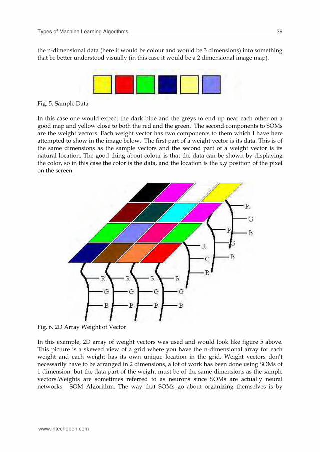
Types of Machine Learning Algorithms 39
that the centres settle down to a compromise representation of the cases which cause that neuron to win. The topological ordering property is achieved by adding the concept of a neighbourhood to the algorithm. The neighbourhood is a set of neurons surrounding the winning neuron. The neighbourhood, like the learning rate, decays over time, so that initially quite a large number of neurons belong to the neighbourhood (perhaps almost the entire topological map); in the latter stages the neighbourhood will be zero (i.e., consists solely of the winning neuron itself). In the Kohonen algorithm, the adjustment of neurons is actually applied not just to the winning neuron, but to all the members of the current neighbourhood. The effect of this neighbourhood update is that initially quite large areas of the network are "dragged towards" training cases - and dragged quite substantially. The network develops a crude topological ordering, with similar cases activating clumps of neurons in the topological map. As epochs pass the learning rate and neighbourhood both decrease, so that finer distinctions within areas of the map can be drawn, ultimately resulting in fine-tuning of individual neurons. Often, training is deliberately conducted in two distinct phases: a relatively short phase with high learning rates and neighbourhood, and a long phase with low learning rate and zero or near-zero neighbourhoods. Once the network has been trained to recognize structure in the data, it can be used as a visualization tool to examine the data. The Win Frequencies Datasheet (counts of the number of times each neuron wins when training cases are executed) can be examined to see if distinct clusters have formed on the map. Individual cases are executed and the topological map observed, to see if some meaning can be assigned to the clusters (this usually involves referring back to the original application area, so that the relationship between clustered cases can be established). Once clusters are identified, neurons in the topological map are labelled to indicate their meaning (sometimes individual cases may be labelled, too). Once the topological map has been built up in this way, new cases can be submitted to the network. If the winning neuron has been labelled with a class name, the network can perform classification. If not, the network is regarded as undecided. SOFM networks also make use of the accept threshold, when performing classification. Since the activation level of a neuron in a SOFM network is the distance of the neuron from the input case, the accept threshold acts as a maximum recognized distance. If the activation of the winning neuron is greater than this distance, the SOFM network is regarded as undecided. Thus, by labelling all neurons and setting the accept threshold appropriately, a SOFM network can act as a novelty detector (it reports undecided only if the input case is sufficiently dissimilar to all radial units). SOFM networks as expressed by Kohonen (Kohonen, 1997) are inspired by some known properties of the brain. The cerebral cortex is actually a large flat sheet (about 0.5m squared; it is folded up into the familiar convoluted shape only for convenience in fitting into the skull!) with known topological properties (for example, the area corresponding to the hand is next to the arm, and a distorted human frame can be topologically mapped out in two dimensions on its surface).
1.4 Grouping Data Using Self Organise Map The first part of a SOM is the data. Above are some examples of 3 dimensional data which are commonly used when experimenting with SOMs. Here the colours are represented in three dimensions (red, blue, and green.) The idea of the self-organizing maps is to project
the n-dimensional data (here it would be colour and would be 3 dimensions) into something that be better understood visually (in this case it would be a 2 dimensional image map).
Fig. 5. Sample Data In this case one would expect the dark blue and the greys to end up near each other on a good map and yellow close to both the red and the green. The second components to SOMs are the weight vectors. Each weight vector has two components to them which I have here attempted to show in the image below. The first part of a weight vector is its data. This is of the same dimensions as the sample vectors and the second part of a weight vector is its natural location. The good thing about colour is that the data can be shown by displaying the color, so in this case the color is the data, and the location is the x,y position of the pixel on the screen.
Fig. 6. 2D Array Weight of Vector
In this example, 2D array of weight vectors was used and would look like figure 5 above. This picture is a skewed view of a grid where you have the n-dimensional array for each weight and each weight has its own unique location in the grid. Weight vectors don’t necessarily have to be arranged in 2 dimensions, a lot of work has been done using SOMs of 1 dimension, but the data part of the weight must be of the same dimensions as the sample vectors.Weights are sometimes referred to as neurons since SOMs are actually neural networks. SOM Algorithm. The way that SOMs go about organizing themselves is by
www.intechopen.com
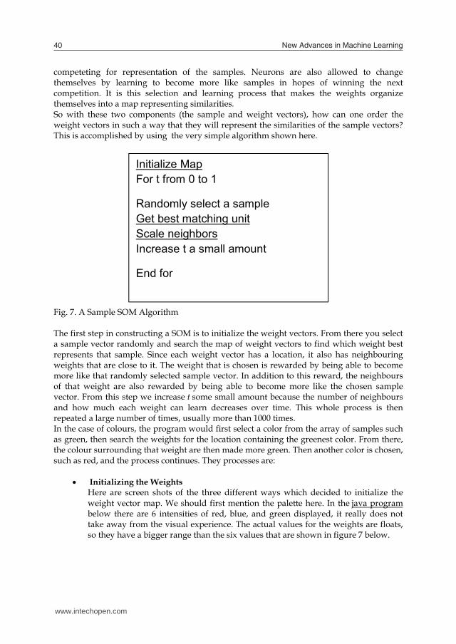
New Advances in Machine Learning40
competeting for representation of the samples. Neurons are also allowed to change themselves by learning to become more like samples in hopes of winning the next competition. It is this selection and learning process that makes the weights organize themselves into a map representing similarities. So with these two components (the sample and weight vectors), how can one order the weight vectors in such a way that they will represent the similarities of the sample vectors? This is accomplished by using the very simple algorithm shown here.
Fig. 7. A Sample SOM Algorithm The first step in constructing a SOM is to initialize the weight vectors. From there you select a sample vector randomly and search the map of weight vectors to find which weight best represents that sample. Since each weight vector has a location, it also has neighbouring weights that are close to it. The weight that is chosen is rewarded by being able to become more like that randomly selected sample vector. In addition to this reward, the neighbours of that weight are also rewarded by being able to become more like the chosen sample vector. From this step we increase t some small amount because the number of neighbours and how much each weight can learn decreases over time. This whole process is then repeated a large number of times, usually more than 1000 times. In the case of colours, the program would first select a color from the array of samples such as green, then search the weights for the location containing the greenest color. From there, the colour surrounding that weight are then made more green. Then another color is chosen, such as red, and the process continues. They processes are:
• Initializing the Weights Here are screen shots of the three different ways which decided to initialize the weight vector map. We should first mention the palette here. In the java program below there are 6 intensities of red, blue, and green displayed, it really does not take away from the visual experience. The actual values for the weights are floats, so they have a bigger range than the six values that are shown in figure 7 below.
Initialize MapFor t from 0 to 1
Randomly select a sampleGet best matching unitScale neighborsIncrease t a small amount
End for
Fig. 8. Weight Values
There are a number of ways to initialize the weight vectors. The first you can see is just give each weight vector random values for its data. A screen of pixels with random red, blue, and green values is shown above on the left. Unfortunately calculating SOMs according to Kohonen (Kohonen, 1997) is very computationally expensive, so there are some variants of initializing the weights so that samples that you know for a fact are not similar start off far away. This way you need less iteration to produce a good map and can save yourself some time. Here we made two other ways to initialize the weights in addition to the random one. This one is just putting red, blue, green, and black at all four corners and having them slowly fade toward the center. This other one is having red, green, and blue equally distant from one another and from the center.
• B. Get Best Matching Unit This is a very simple step, just go through all the weight vectors and calculate the distance from each weight to the chosen sample vector. The weight with the shortest distance is the winner. If there are more than one with the same distance, then the winning weight is chosen randomly among the weights with the shortest distance. There are a number of different ways for determining what distance actually means mathematically. The most common method is to use the Euclidean distance:
www.intechopen.com
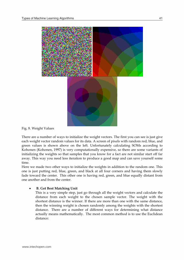
Types of Machine Learning Algorithms 41
competeting for representation of the samples. Neurons are also allowed to change themselves by learning to become more like samples in hopes of winning the next competition. It is this selection and learning process that makes the weights organize themselves into a map representing similarities. So with these two components (the sample and weight vectors), how can one order the weight vectors in such a way that they will represent the similarities of the sample vectors? This is accomplished by using the very simple algorithm shown here.
Fig. 7. A Sample SOM Algorithm The first step in constructing a SOM is to initialize the weight vectors. From there you select a sample vector randomly and search the map of weight vectors to find which weight best represents that sample. Since each weight vector has a location, it also has neighbouring weights that are close to it. The weight that is chosen is rewarded by being able to become more like that randomly selected sample vector. In addition to this reward, the neighbours of that weight are also rewarded by being able to become more like the chosen sample vector. From this step we increase t some small amount because the number of neighbours and how much each weight can learn decreases over time. This whole process is then repeated a large number of times, usually more than 1000 times. In the case of colours, the program would first select a color from the array of samples such as green, then search the weights for the location containing the greenest color. From there, the colour surrounding that weight are then made more green. Then another color is chosen, such as red, and the process continues. They processes are:
• Initializing the Weights Here are screen shots of the three different ways which decided to initialize the weight vector map. We should first mention the palette here. In the java program below there are 6 intensities of red, blue, and green displayed, it really does not take away from the visual experience. The actual values for the weights are floats, so they have a bigger range than the six values that are shown in figure 7 below.
Initialize MapFor t from 0 to 1
Randomly select a sampleGet best matching unitScale neighborsIncrease t a small amount
End for
Fig. 8. Weight Values
There are a number of ways to initialize the weight vectors. The first you can see is just give each weight vector random values for its data. A screen of pixels with random red, blue, and green values is shown above on the left. Unfortunately calculating SOMs according to Kohonen (Kohonen, 1997) is very computationally expensive, so there are some variants of initializing the weights so that samples that you know for a fact are not similar start off far away. This way you need less iteration to produce a good map and can save yourself some time. Here we made two other ways to initialize the weights in addition to the random one. This one is just putting red, blue, green, and black at all four corners and having them slowly fade toward the center. This other one is having red, green, and blue equally distant from one another and from the center.
• B. Get Best Matching Unit This is a very simple step, just go through all the weight vectors and calculate the distance from each weight to the chosen sample vector. The weight with the shortest distance is the winner. If there are more than one with the same distance, then the winning weight is chosen randomly among the weights with the shortest distance. There are a number of different ways for determining what distance actually means mathematically. The most common method is to use the Euclidean distance:
www.intechopen.com
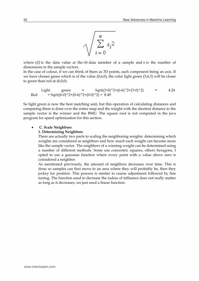
New Advances in Machine Learning42
where x[i] is the data value at the ith data member of a sample and n is the number of dimensions to the sample vectors. In the case of colour, if we can think of them as 3D points, each component being an axis. If we have chosen green which is of the value (0,6,0), the color light green (3,6,3) will be closer to green than red at (6,0,0). Light green = Sqrt((3-0)^2+(6-6)^2+(3-0)^2) = 4.24 Red = Sqrt((6-0)^2+(0-6)^2+(0-0)^2) = 8.49 So light green is now the best matching unit, but this operation of calculating distances and comparing them is done over the entire map and the wieght with the shortest distance to the sample vector is the winner and the BMU. The square root is not computed in the java program for speed optimization for this section.
• C. Scale Neighbors 1. Determining Neighbors There are actually two parts to scaling the neighboring weights: determining which weights are considered as neighbors and how much each weight can become more like the sample vector. The neighbors of a winning weight can be determined using a number of different methods. Some use concentric squares, others hexagons, I opted to use a gaussian function where every point with a value above zero is considered a neighbor. As mentioned previously, the amount of neighbors decreases over time. This is done so samples can first move to an area where they will probably be, then they jockey for position. This process is similar to coarse adjustment followed by fine tuning. The function used to decrease the radius of influence does not really matter as long as it decreases, we just used a linear function.
Fig. 9. A graph of SOM Neighbour’s determination
Figure 8 above shows a plot of the function used. As the time progresses, the base goes towards the centre, so there are less neighbours as time progresses. The initial radius is set really high, some value near the width or height of the map.
2. Learning The second part to scaling the neighbours is the learning function. The winning weight is rewarded with becoming more like the sample vector. The neighbours also become more like the sample vector. An attribute of this learning process is that the farther away the neighbour is from the winning vector, the less it learns. The rate at which the amount a weight can learn decreases and can also be set to whatever you want. I chose to use a gaussian function. This function will return a value ranging between 0 and 1, where each neighbor is then changed using the parametric equation. The new color is:
Current color*(1.-t) + sample vector*t
So in the first iteration, the best matching unit will get a t of 1 for its learning function, so the weight will then come out of this process with the same exact values as the randomly selected sample.
Just as the amount of neighbors a weight has falls off, the amount a weight can learn also decreases with time. On the first iteration, the winning weight becomes the sample vector since t has a full range of from 0 to 1. Then as time progresses, the winning weight becomes slightly more like the sample where the maximum value of t decreases. The rate at which
www.intechopen.com
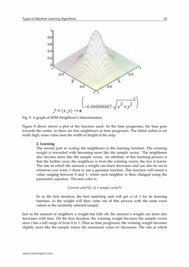
Types of Machine Learning Algorithms 43
where x[i] is the data value at the ith data member of a sample and n is the number of dimensions to the sample vectors. In the case of colour, if we can think of them as 3D points, each component being an axis. If we have chosen green which is of the value (0,6,0), the color light green (3,6,3) will be closer to green than red at (6,0,0). Light green = Sqrt((3-0)^2+(6-6)^2+(3-0)^2) = 4.24 Red = Sqrt((6-0)^2+(0-6)^2+(0-0)^2) = 8.49 So light green is now the best matching unit, but this operation of calculating distances and comparing them is done over the entire map and the wieght with the shortest distance to the sample vector is the winner and the BMU. The square root is not computed in the java program for speed optimization for this section.
• C. Scale Neighbors 1. Determining Neighbors There are actually two parts to scaling the neighboring weights: determining which weights are considered as neighbors and how much each weight can become more like the sample vector. The neighbors of a winning weight can be determined using a number of different methods. Some use concentric squares, others hexagons, I opted to use a gaussian function where every point with a value above zero is considered a neighbor. As mentioned previously, the amount of neighbors decreases over time. This is done so samples can first move to an area where they will probably be, then they jockey for position. This process is similar to coarse adjustment followed by fine tuning. The function used to decrease the radius of influence does not really matter as long as it decreases, we just used a linear function.
Fig. 9. A graph of SOM Neighbour’s determination
Figure 8 above shows a plot of the function used. As the time progresses, the base goes towards the centre, so there are less neighbours as time progresses. The initial radius is set really high, some value near the width or height of the map.
2. Learning The second part to scaling the neighbours is the learning function. The winning weight is rewarded with becoming more like the sample vector. The neighbours also become more like the sample vector. An attribute of this learning process is that the farther away the neighbour is from the winning vector, the less it learns. The rate at which the amount a weight can learn decreases and can also be set to whatever you want. I chose to use a gaussian function. This function will return a value ranging between 0 and 1, where each neighbor is then changed using the parametric equation. The new color is:
Current color*(1.-t) + sample vector*t
So in the first iteration, the best matching unit will get a t of 1 for its learning function, so the weight will then come out of this process with the same exact values as the randomly selected sample.
Just as the amount of neighbors a weight has falls off, the amount a weight can learn also decreases with time. On the first iteration, the winning weight becomes the sample vector since t has a full range of from 0 to 1. Then as time progresses, the winning weight becomes slightly more like the sample where the maximum value of t decreases. The rate at which
www.intechopen.com
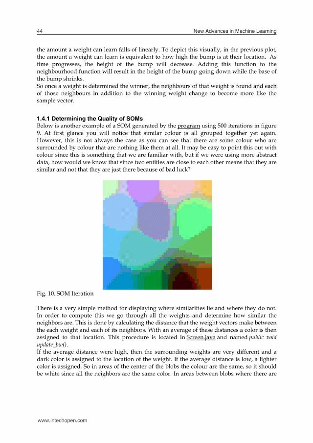
New Advances in Machine Learning44
the amount a weight can learn falls of linearly. To depict this visually, in the previous plot, the amount a weight can learn is equivalent to how high the bump is at their location. As time progresses, the height of the bump will decrease. Adding this function to the neighbourhood function will result in the height of the bump going down while the base of the bump shrinks. So once a weight is determined the winner, the neighbours of that weight is found and each of those neighbours in addition to the winning weight change to become more like the sample vector.
1.4.1 Determining the Quality of SOMs Below is another example of a SOM generated by the program using 500 iterations in figure 9. At first glance you will notice that similar colour is all grouped together yet again. However, this is not always the case as you can see that there are some colour who are surrounded by colour that are nothing like them at all. It may be easy to point this out with colour since this is something that we are familiar with, but if we were using more abstract data, how would we know that since two entities are close to each other means that they are similar and not that they are just there because of bad luck?
Fig. 10. SOM Iteration
There is a very simple method for displaying where similarities lie and where they do not. In order to compute this we go through all the weights and determine how similar the neighbors are. This is done by calculating the distance that the weight vectors make between the each weight and each of its neighbors. With an average of these distances a color is then assigned to that location. This procedure is located in Screen.java and named public void update_bw(). If the average distance were high, then the surrounding weights are very different and a dark color is assigned to the location of the weight. If the average distance is low, a lighter color is assigned. So in areas of the center of the blobs the colour are the same, so it should be white since all the neighbors are the same color. In areas between blobs where there are
similarities it should be not white, but a light grey. Areas where the blobs are physically close to each other, but are not similar at all there should be black. See Figure 8 below
Fig. 11. A sample allocation of Weight in Colour
As shown above, the ravines of black show where the colour may be physically close to each other on the map, but are very different from each other when it comes to the actual values of the weights. Areas where there is a light grey between the blobs represent a true similarity. In the pictures above, in the bottom right there is black surrounded by colour which are not very similar to it. When looking at the black and white similarity SOM, it shows that black is not similar to the other colour because there are lines of black representing no similarity between those two colour. Also in the top corner there is pink and nearby is a light green which are not very near each other in reality, but near each other on the colored SOM. Looking at the black and white SOM, it clearly shows that the two not very similar by having black in between the two colour. With these average distances used to make the black and white map, we can actually assign each SOM a value that determines how good the image represents the similarities of the samples by simply adding these averages.
1.4.2 Advantages and Disadvantages of SOM Self organise map has the following advantages:
• Probably the best thing about SOMs that they are very easy to understand. It’s very simple, if they are close together and there is grey connecting them, then they are similar. If there is a black ravine between them, then they are different. Unlike Multidimensional Scaling or N-land, people can quickly pick up on how to use them in an effective manner.
• Another great thing is that they work very well. As I have shown you they classify data well and then are easily evaluate for their own quality so you can actually calculated how good a map is and how strong the similarities between objects are.
These are the disadvantages:
www.intechopen.com
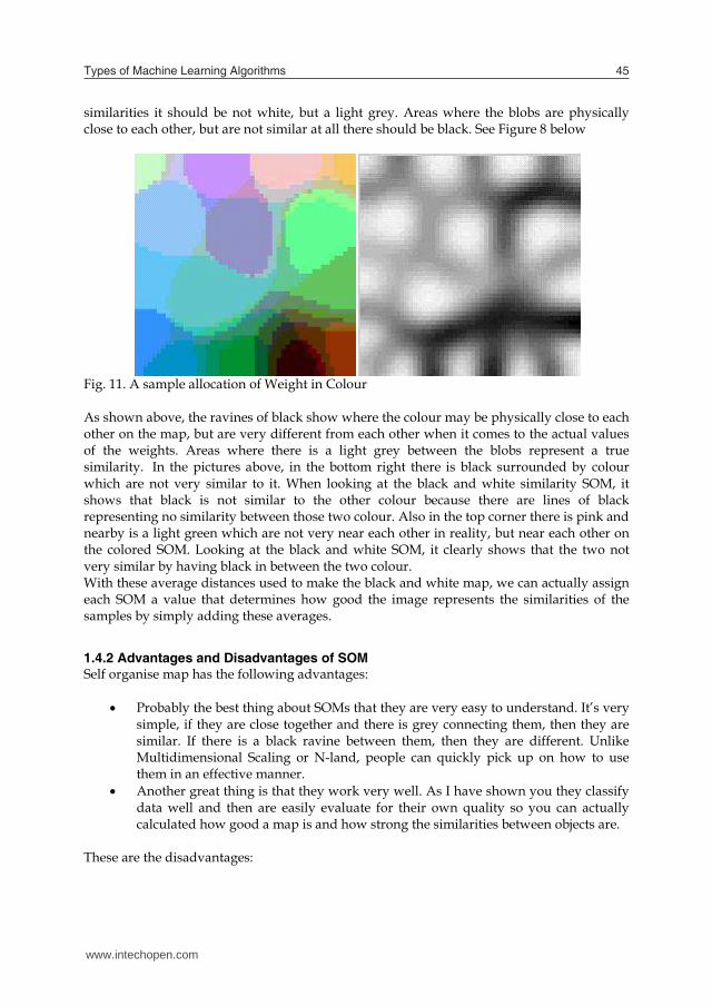
Types of Machine Learning Algorithms 45
the amount a weight can learn falls of linearly. To depict this visually, in the previous plot, the amount a weight can learn is equivalent to how high the bump is at their location. As time progresses, the height of the bump will decrease. Adding this function to the neighbourhood function will result in the height of the bump going down while the base of the bump shrinks. So once a weight is determined the winner, the neighbours of that weight is found and each of those neighbours in addition to the winning weight change to become more like the sample vector.
1.4.1 Determining the Quality of SOMs Below is another example of a SOM generated by the program using 500 iterations in figure 9. At first glance you will notice that similar colour is all grouped together yet again. However, this is not always the case as you can see that there are some colour who are surrounded by colour that are nothing like them at all. It may be easy to point this out with colour since this is something that we are familiar with, but if we were using more abstract data, how would we know that since two entities are close to each other means that they are similar and not that they are just there because of bad luck?
Fig. 10. SOM Iteration
There is a very simple method for displaying where similarities lie and where they do not. In order to compute this we go through all the weights and determine how similar the neighbors are. This is done by calculating the distance that the weight vectors make between the each weight and each of its neighbors. With an average of these distances a color is then assigned to that location. This procedure is located in Screen.java and named public void update_bw(). If the average distance were high, then the surrounding weights are very different and a dark color is assigned to the location of the weight. If the average distance is low, a lighter color is assigned. So in areas of the center of the blobs the colour are the same, so it should be white since all the neighbors are the same color. In areas between blobs where there are
similarities it should be not white, but a light grey. Areas where the blobs are physically close to each other, but are not similar at all there should be black. See Figure 8 below
Fig. 11. A sample allocation of Weight in Colour
As shown above, the ravines of black show where the colour may be physically close to each other on the map, but are very different from each other when it comes to the actual values of the weights. Areas where there is a light grey between the blobs represent a true similarity. In the pictures above, in the bottom right there is black surrounded by colour which are not very similar to it. When looking at the black and white similarity SOM, it shows that black is not similar to the other colour because there are lines of black representing no similarity between those two colour. Also in the top corner there is pink and nearby is a light green which are not very near each other in reality, but near each other on the colored SOM. Looking at the black and white SOM, it clearly shows that the two not very similar by having black in between the two colour. With these average distances used to make the black and white map, we can actually assign each SOM a value that determines how good the image represents the similarities of the samples by simply adding these averages.
1.4.2 Advantages and Disadvantages of SOM Self organise map has the following advantages:
• Probably the best thing about SOMs that they are very easy to understand. It’s very simple, if they are close together and there is grey connecting them, then they are similar. If there is a black ravine between them, then they are different. Unlike Multidimensional Scaling or N-land, people can quickly pick up on how to use them in an effective manner.
• Another great thing is that they work very well. As I have shown you they classify data well and then are easily evaluate for their own quality so you can actually calculated how good a map is and how strong the similarities between objects are.
These are the disadvantages:
www.intechopen.com
New Advances in Machine Learning46
• One major problem with SOMs is getting the right data. Unfortunately you need a value for each dimension of each member of samples in order to generate a map. Sometimes this simply is not possible and often it is very difficult to acquire all of this data so this is a limiting feature to the use of SOMs often referred to as missing data.
• Another problem is that every SOM is different and finds different similarities among the sample vectors. SOMs organize sample data so that in the final product, the samples are usually surrounded by similar samples, however similar samples are not always near each other. If you have a lot of shades of purple, not always will you get one big group with all the purples in that cluster, sometimes the clusters will get split and there will be two groups of purple. Using colour we could tell that those two groups in reality are similar and that they just got split, but with most data, those two clusters will look totally unrelated. So a lot of maps need to be constructed in order to get one final good map.
• The final major problem with SOMs is that they are very computationally expensive which is a major drawback since as the dimensions of the data increases, dimension reduction visualization techniques become more important, but unfortunately then time to compute them also increases. For calculating that black and white similarity map, the more neighbours you use to calculate the distance the better similarity map you will get, but the number of distances the algorithm needs to compute increases exponentially.
2. References
Allix, N. M. (2003, April). Epistemology And Knowledge Management Concepts And Practices. Journal of Knowledge Management Practice .
Alpaydin, E. (2004). Introduction to Machine Learning. Massachusetts, USA: MIT Press. Anderson, J. R. (1995). Learning and Memory. Wiley, New York, USA. Anil Mathur, G. P. (1999). Socialization influences on preparation for later life. Journal of
Marketing Practice: Applied Marketing Science , 5 (6,7,8), 163 - 176. Ashby, W. R. (1960). Design of a Brain, The Origin of Adaptive Behaviour. John Wiley and Son. Batista, G. &. (2003). An Analysis of Four Missing Data Treatment Methods for Suppervised
Learning. Applied Artificial Intelligence , 17, 519-533. Bishop, C. M. (1995). Neural Networks for Pattern Recognition. Oxford, England: Oxford
University Press. Bishop, C. M. (2006). Pattern Recognition and Machine Learning (Information Science and
Statistics). New York, New York: Springer Science and Business Media. Block H, D. (1961). The Perceptron: A Model of Brian Functioning. 34 (1), 123-135. Carling, A. (1992). Introducing Neural Networks . Wilmslow, UK: Sigma Press. D. Michie, D. J. (1994). Machine Learning, Neural and Statistical Classification. Prentice Hall Inc. Fausett, L. (19994). Fundamentals of Neural Networks. New York: Prentice Hall. Forsyth, R. S. (1990). The strange story of the Perceptron. Artificial Intelligence Review , 4 (2),
147-155. Friedberg, R. M. (1958). A learning machine: Part, 1. IBM Journal , 2-13. Ghahramani, Z. (2008). Unsupervised learning algorithms are designed to extract structure
from data. 178, pp. 1-8. IOS Press.
Gillies, D. (1996). Artificial Intelligence and Scientific Method. OUP Oxford. Haykin, S. (19994). Neural Networks: A Comprehensive Foundation. New York: Macmillan
Publishing. Hodge, V. A. (2004). A Survey of Outlier Detection Methodologies. Artificial Intelligence
Review , 22 (2), 85-126. Holland, J. (1980). Adaptive Algorithms for Discovering and Using General Patterns in
Growing Knowledge Bases Policy Analysis and Information Systems. 4 (3). Hunt, E. B. (1966). Experiment in Induction. Ian H. Witten, E. F. (2005). Data Mining Practical Machine Learning and Techniques (Second
edition ed.). Morgan Kaufmann. Jaime G. Carbonell, R. S. (1983). Machine Learning: A Historical and Methodological
Analysis. Association for the Advancement of Artificial Intelligence , 4 (3), 1-10. Kohonen, T. (1997). Self-Organizating Maps. Luis Gonz, l. A. (2005). Unified dual for bi-class SVM approaches. Pattern Recognition , 38
(10), 1772-1774. McCulloch, W. S. (1943). A logical calculus of the ideas immanent in nervous activity. Bull.
Math. Biophysics , 115-133. Mitchell, T. M. (2006). The Discipline of Machine Learning. Machine Learning Department
technical report CMU-ML-06-108, Carnegie Mellon University. Mooney, R. J. (2000). Learning Language in Logic. In L. N. Science, Learning for Semantic
Interpretation: Scaling Up without Dumbing Down (pp. 219-234). Springer Berlin / Heidelberg.
Mostow, D. (1983). Transforming declarative advice into effective procedures: a heuristic search cxamplc In I?. S. Michalski,. Tioga Press.
Nilsson, N. J. (1982). Principles of Artificial Intelligence (Symbolic Computation / Artificial Intelligence). Springer.
Oltean, M. (2005). Evolving Evolutionary Algorithms Using Linear Genetic Programming. 13 (3), 387 - 410 .
Orlitsky, A., Santhanam, N., Viswanathan, K., & Zhang, J. (2005). Convergence of profile based estimators. Proceedings of International Symposium on Information Theory. Proceedings. International Symposium on, pp. 1843 - 1847. Adelaide, Australia: IEEE.
Patterson, D. (19996). Artificial Neural Networks. Singapore: Prentice Hall. R. S. Michalski, T. J. (1983). Learning from Observation: Conceptual Clustering. TIOGA
Publishing Co. Rajesh P. N. Rao, B. A. (2002). Probabilistic Models of the Brain. MIT Press. Rashevsky, N. (1948). Mathematical Biophysics:Physico-Mathematical Foundations of Biology.
Chicago: Univ. of Chicago Press. Richard O. Duda, P. E. (2000). Pattern Classification (2nd Edition ed.). Richard S. Sutton, A. G. (1998). Reinforcement Learning. MIT Press. Ripley, B. (1996). Pattern Recognition and Neural Networks. Cambridge University Press. Rosenblatt, F. (1958). The perceptron: a probabilistic model for information storage and
organization in the brain . Psychological Review , 65 (6), 386-408. Russell, S. J. (2003). Artificial Intelligence: A Modern Approach (2nd Edition ed.). Upper Saddle
River, NJ, NJ, USA: Prentice Hall. Ryszard S. Michalski, J. G. (1955). Machine Learning: An Artificial Intelligence Approach
(Volume I). Morgan Kaufmann .
www.intechopen.com
Types of Machine Learning Algorithms 47
• One major problem with SOMs is getting the right data. Unfortunately you need a value for each dimension of each member of samples in order to generate a map. Sometimes this simply is not possible and often it is very difficult to acquire all of this data so this is a limiting feature to the use of SOMs often referred to as missing data.
• Another problem is that every SOM is different and finds different similarities among the sample vectors. SOMs organize sample data so that in the final product, the samples are usually surrounded by similar samples, however similar samples are not always near each other. If you have a lot of shades of purple, not always will you get one big group with all the purples in that cluster, sometimes the clusters will get split and there will be two groups of purple. Using colour we could tell that those two groups in reality are similar and that they just got split, but with most data, those two clusters will look totally unrelated. So a lot of maps need to be constructed in order to get one final good map.
• The final major problem with SOMs is that they are very computationally expensive which is a major drawback since as the dimensions of the data increases, dimension reduction visualization techniques become more important, but unfortunately then time to compute them also increases. For calculating that black and white similarity map, the more neighbours you use to calculate the distance the better similarity map you will get, but the number of distances the algorithm needs to compute increases exponentially.
2. References
Allix, N. M. (2003, April). Epistemology And Knowledge Management Concepts And Practices. Journal of Knowledge Management Practice .
Alpaydin, E. (2004). Introduction to Machine Learning. Massachusetts, USA: MIT Press. Anderson, J. R. (1995). Learning and Memory. Wiley, New York, USA. Anil Mathur, G. P. (1999). Socialization influences on preparation for later life. Journal of
Marketing Practice: Applied Marketing Science , 5 (6,7,8), 163 - 176. Ashby, W. R. (1960). Design of a Brain, The Origin of Adaptive Behaviour. John Wiley and Son. Batista, G. &. (2003). An Analysis of Four Missing Data Treatment Methods for Suppervised
Learning. Applied Artificial Intelligence , 17, 519-533. Bishop, C. M. (1995). Neural Networks for Pattern Recognition. Oxford, England: Oxford
University Press. Bishop, C. M. (2006). Pattern Recognition and Machine Learning (Information Science and
Statistics). New York, New York: Springer Science and Business Media. Block H, D. (1961). The Perceptron: A Model of Brian Functioning. 34 (1), 123-135. Carling, A. (1992). Introducing Neural Networks . Wilmslow, UK: Sigma Press. D. Michie, D. J. (1994). Machine Learning, Neural and Statistical Classification. Prentice Hall Inc. Fausett, L. (19994). Fundamentals of Neural Networks. New York: Prentice Hall. Forsyth, R. S. (1990). The strange story of the Perceptron. Artificial Intelligence Review , 4 (2),
147-155. Friedberg, R. M. (1958). A learning machine: Part, 1. IBM Journal , 2-13. Ghahramani, Z. (2008). Unsupervised learning algorithms are designed to extract structure
from data. 178, pp. 1-8. IOS Press.
Gillies, D. (1996). Artificial Intelligence and Scientific Method. OUP Oxford. Haykin, S. (19994). Neural Networks: A Comprehensive Foundation. New York: Macmillan
Publishing. Hodge, V. A. (2004). A Survey of Outlier Detection Methodologies. Artificial Intelligence
Review , 22 (2), 85-126. Holland, J. (1980). Adaptive Algorithms for Discovering and Using General Patterns in
Growing Knowledge Bases Policy Analysis and Information Systems. 4 (3). Hunt, E. B. (1966). Experiment in Induction. Ian H. Witten, E. F. (2005). Data Mining Practical Machine Learning and Techniques (Second
edition ed.). Morgan Kaufmann. Jaime G. Carbonell, R. S. (1983). Machine Learning: A Historical and Methodological
Analysis. Association for the Advancement of Artificial Intelligence , 4 (3), 1-10. Kohonen, T. (1997). Self-Organizating Maps. Luis Gonz, l. A. (2005). Unified dual for bi-class SVM approaches. Pattern Recognition , 38
(10), 1772-1774. McCulloch, W. S. (1943). A logical calculus of the ideas immanent in nervous activity. Bull.
Math. Biophysics , 115-133. Mitchell, T. M. (2006). The Discipline of Machine Learning. Machine Learning Department
technical report CMU-ML-06-108, Carnegie Mellon University. Mooney, R. J. (2000). Learning Language in Logic. In L. N. Science, Learning for Semantic
Interpretation: Scaling Up without Dumbing Down (pp. 219-234). Springer Berlin / Heidelberg.
Mostow, D. (1983). Transforming declarative advice into effective procedures: a heuristic search cxamplc In I?. S. Michalski,. Tioga Press.
Nilsson, N. J. (1982). Principles of Artificial Intelligence (Symbolic Computation / Artificial Intelligence). Springer.
Oltean, M. (2005). Evolving Evolutionary Algorithms Using Linear Genetic Programming. 13 (3), 387 - 410 .
Orlitsky, A., Santhanam, N., Viswanathan, K., & Zhang, J. (2005). Convergence of profile based estimators. Proceedings of International Symposium on Information Theory. Proceedings. International Symposium on, pp. 1843 - 1847. Adelaide, Australia: IEEE.
Patterson, D. (19996). Artificial Neural Networks. Singapore: Prentice Hall. R. S. Michalski, T. J. (1983). Learning from Observation: Conceptual Clustering. TIOGA
Publishing Co. Rajesh P. N. Rao, B. A. (2002). Probabilistic Models of the Brain. MIT Press. Rashevsky, N. (1948). Mathematical Biophysics:Physico-Mathematical Foundations of Biology.
Chicago: Univ. of Chicago Press. Richard O. Duda, P. E. (2000). Pattern Classification (2nd Edition ed.). Richard S. Sutton, A. G. (1998). Reinforcement Learning. MIT Press. Ripley, B. (1996). Pattern Recognition and Neural Networks. Cambridge University Press. Rosenblatt, F. (1958). The perceptron: a probabilistic model for information storage and
organization in the brain . Psychological Review , 65 (6), 386-408. Russell, S. J. (2003). Artificial Intelligence: A Modern Approach (2nd Edition ed.). Upper Saddle
River, NJ, NJ, USA: Prentice Hall. Ryszard S. Michalski, J. G. (1955). Machine Learning: An Artificial Intelligence Approach
(Volume I). Morgan Kaufmann .
www.intechopen.com
New Advances in Machine Learning48
Ryszard S. Michalski, J. G. (1955). Machine Learning: An Artificial Intelligence Approach. Selfridge, O. G. (1959). Pandemonium: a paradigm for learning. In The mechanisation of
thought processes. H.M.S.O., London. London. Sleeman, D. H. (1983). Inferring Student Models for Intelligent CAI. Machine Learning. Tioga
Press. Tapas Kanungo, D. M. (2002). A local search approximation algorithm for k-means
clustering. Proceedings of the eighteenth annual symposium on Computational geometry (pp. 10-18). Barcelona, Spain : ACM Press.
Timothy Jason Shepard, P. J. (1998). Decision Fusion Using a Multi-Linear Classifier . In Proceedings of the International Conference on Multisource-Multisensor Information Fusion.
Tom, M. (1997). Machibe Learning. Machine Learning, Tom Mitchell, McGraw Hill, 1997: McGraw Hill.
Trevor Hastie, R. T. (2001). The Elements of Statistical Learning. New york, NY, USA: Springer Science and Business Media.
Widrow, B. W. (2007). Adaptive Inverse Control: A Signal Processing Approach. Wiley-IEEE Press.
Y. Chali, S. R. (2009). Complex Question Answering: Unsupervised Learning Approaches and Experiments. Journal of Artificial Intelligent Research , 1-47.
Yu, L. L. (2004, October). Efficient feature Selection via Analysis of Relevance and Redundacy. JMLR , 1205-1224.
Zhang, S. Z. (2002). Data Preparation for Data Mining. Applied Artificial Intelligence. 17, 375 - 381.
www.intechopen.com
New Advances in Machine LearningEdited by Yagang Zhang
ISBN 978-953-307-034-6Hard cover, 366 pagesPublisher InTechPublished online 01, February, 2010Published in print edition February, 2010
InTech EuropeUniversity Campus STeP Ri Slavka Krautzeka 83/A 51000 Rijeka, Croatia Phone: +385 (51) 770 447 Fax: +385 (51) 686 166www.intechopen.com
InTech ChinaUnit 405, Office Block, Hotel Equatorial Shanghai No.65, Yan An Road (West), Shanghai, 200040, China
Phone: +86-21-62489820 Fax: +86-21-62489821
The purpose of this book is to provide an up-to-date and systematical introduction to the principles andalgorithms of machine learning. The definition of learning is broad enough to include most tasks that wecommonly call “learning” tasks, as we use the word in daily life. It is also broad enough to encompasscomputers that improve from experience in quite straightforward ways. The book will be of interest to industrialengineers and scientists as well as academics who wish to pursue machine learning. The book is intended forboth graduate and postgraduate students in fields such as computer science, cybernetics, system sciences,engineering, statistics, and social sciences, and as a reference for software professionals and practitioners.The wide scope of the book provides a good introduction to many approaches of machine learning, and it isalso the source of useful bibliographical information.
How to referenceIn order to correctly reference this scholarly work, feel free to copy and paste the following:
Taiwo Oladipupo Ayodele (2010). Types of Machine Learning Algorithms, New Advances in Machine Learning,Yagang Zhang (Ed.), ISBN: 978-953-307-034-6, InTech, Available from:http://www.intechopen.com/books/new-advances-in-machine-learning/types-of-machine-learning-algorithms