tutorial on seismic interferometry - school of geosciences

TP

K

etaoaoittgtc

©

G1

EOPHYSICS, VOL. 75, NO. 5 �SEPTEMBER-OCTOBER 2010�; P. 75A211–75A227, 10 FIGS.0.1190/1.3463440

utorial on seismic interferometry:art 2 — Underlying theory and new advances

ees Wapenaar1, Evert Slob1, Roel Snieder2, and Andrew Curtis3

esoiltatttihtste

ABSTRACT

In the 1990s, the method of time-reversed acoustics was devel-oped. This method exploits the fact that the acoustic wave equa-tion for a lossless medium is invariant for time reversal. When ul-trasonic responses recorded by piezoelectric transducers are re-versed in time and fed simultaneously as source signals to thetransducers, they focus at the position of the original source, evenwhen the medium is very complex. In seismic interferometry thetime-reversed responses are not physically sent into the earth, butthey are convolved with other measured responses. The effect isessentially the same: The time-reversed signals focus and createa virtual source which radiates waves into the medium that aresubsequently recorded by receivers. A mathematical derivation,based on reciprocity theory, formalizes this principle: The cross-correlation of responses at two receivers, integrated over differ-

amtbs

R

oa

Septeme Netheo, U.S.

l: andre

e in the a

75A211

Downloaded 15 Sep 2010 to 129.215.6.61. Redistribution subject to S

nt sources, gives the Green’s function emitted by a virtualource at the position of one of the receivers and observed by thether receiver. This Green’s function representation for seismicnterferometry is based on the assumption that the medium isossless and nonmoving. Recent developments, circumventinghese assumptions, include interferometric representations forttenuating and/or moving media, as well as unified representa-ions for waves and diffusion phenomena, bending waves, quan-um mechanical scattering, potential fields, elastodynamic, elec-romagnetic, poroelastic, and electroseismic waves. Significantmprovements in the quality of the retrieved Green’s functionsave been obtained with interferometry by deconvolution. Arace-by-trace deconvolution process compensates for complexource functions and the attenuation of the medium. Interferome-ry by multidimensional deconvolution also compensates for theffects of one-sided and/or irregular illumination.

INTRODUCTION

In Part 1, we discussed the basic principles of seismic interferom-try �also known as Green’s function retrieval4� using mainly heuris-ic arguments. In Part 2, we continue our discussion, starting with annalysis of the relation between seismic interferometry and the fieldf time-reversed acoustics, pioneered by Fink �1992, 1997�. Thisnalysis includes a heuristic discussion of the virtual-source methodf Bakulin and Calvert �2004, 2006� and a review of an elegant phys-cal derivation by Derode et al. �2003a, b� of Green’s function re-rieval by crosscorrelation.After that, we review exact Green’s func-ion representations for seismic interferometry in arbitrary inhomo-eneous, anisotropic lossless solids �Wapenaar, 2004� and discusshe approximations that lead to the commonly used expressions. Weonclude with an overview of recent and new advances, including

Manuscript received by the Editor 30 November 2009; published online 141Delft University of Technology, Department of Geotechnology, Delft, Th2Colorado School of Mines, Center for Wave Phenomena, Golden, Colorad3University of Edinburgh, School of GeoSciences, Edinburgh, U.K. E-mai2010 Society of Exploration Geophysicists.All rights reserved.4By “Green’s function,” we mean the response of an impulsive point sourc

pproaches that account for attenuating and/or nonreciprocal media,ethods for obtaining virtual receivers or virtual reflectors, the rela-

ionship with imaging theory, and, last but not least, interferometryy deconvolution. The discussion of each of these advances is neces-arily brief, but we include many references for further reading.

INTERFEROMETRY AND TIME-REVERSEDACOUSTICS

eview of time-reversed acoustics

In the early 1990s, Mathias Fink and coworkers at the Universityf Paris VII initiated a new field of research called time-reversedcoustics �Fink, 1992, 1997; Derode et al., 1995; Draeger and Fink,

ber 2010.rlands. E-mail: [email protected]; [email protected]. E-mail: [email protected]@ed.ac.uk.

ctual medium rather than in a background medium.

EG license or copyright; see Terms of Use at http://segdl.org/

1fio

wrztt2�u0euitTdstssrur

pohtfnpbeos

ptojHtttarfi

nvcofeca

oesueoia

vCttomw

A

a

b

F1dtc

75A212 Wapenaar et al.

999; Fink and Prada, 2001�. Here, we briefly review this researcheld; in the next sections, we discuss the links with seismic interfer-metry.

Time-reversed acoustics makes use of the fact that the acousticave equation for a lossless acoustic medium is invariant under time

eversal �because it only contains even-order time derivatives, i.e.,eroth and second order�. This means that when u�x,t� is a solution,hen u�x,�t� is a solution as well. Figure 1 illustrates the principle inhe context of an ultrasonic experiment �Derode et al., 1995; Fink,006�. A piezoelectric source at A in Figure 1a emits a short pulseduration of 1 �s� that propagates through a highly scattering medi-m �a set of 2000 randomly distributed steel rods with a diameter of.8 mm�. The transmitted wavefield is received by an array of piezo-lectric transducers at B. The received traces �three are shown in Fig-re 1a� exhibit a long coda ��200 �s� because of multiple scatter-ng between the rods. Next, the traces are reversed in time and simul-aneously fed as source signals to the transducers at B �Figure 1b�.his time-reversed wavefield propagates through the scattering me-ium and focuses at the position of the original source. Figure 1chows the received signal at the original source position; the dura-ion is of the same order as the original signal ��1 �s�. Figure 1dhows beam profiles around the source position �amplitudes mea-ured along the x-axis denoted in Figure 1b�. The narrow beam is theesult of this experiment �back propagation via the scattering medi-m�, whereas the wide beam was obtained when the steel rods wereemoved.

The resolution is impressive; at the time, the stability of this ex-eriment amazed many researchers. From a numerical experiment,ne might expect such good reconstruction; however, when wavesave scattered by tens to hundreds of scatterers in a real experiment,he fact that the wavefield refocuses at the original source point isascinating. Snieder and Scales �1998� have analyzed this phenome-on in detail. In their analysis, they compare wave scattering witharticle scattering. They show for their model that, whereas particlesehave chaotically after having encountered typically eight scatter-rs, waves remain stable after 30 or more scatterers. The instabilityf particle scattering is explained by the fact that particles follow aingle trajectory.Asmall disturbance in initial conditions or scatterer

0

–5

–10

–15

–20

–25–3 –2 –1

10.5

0–0.5–1

–50 –25

Distance fro

Tim

Am

plitu

de(d

B)

Nor

mal

ized

ampl

itude

A

B

B

(First step)

(Second step)

x-axis

)

)

c)

d)

igure 1. Time-reversed acoustics in a strongly scattering random me995; Fink, 2006�. �a� The source at A emits a short pulse that propagom medium. The scattered waves are recorded by the array at B. �b�he time-reversed signals, which, after back propagation through the rus at A. �c� The back-propagated response at A. �d� Beam profiles aro


ositions causes the particle to follow a completely different trajec-ory after only a few encounters with the scatterers. Waves, on thether hand, have a finite wavelength and travel along all possible tra-ectories, visiting all of the scatterers in all possible combinations.ence, a small perturbation in initial conditions or scatterer posi-

ions has a much less dramatic effect for wave scattering than for par-icle scattering. Consequently, wave-propagation experimentshrough a strongly scattering medium have a high degree of repeat-bility. Combined with the invariance of the wave equation for timeeversal, this explains the excellent reproduction of the source wave-eld after back propagation through the scattering medium.As a historical side note, the idea of emitting time-reversed sig-

als into a system was proposed and implemented in the 1960s �Par-ulescu, 1961, 1995�. This was a single-channel method, aiming toompress a complicated response at a detector �for example, in ancean waveguide� into a single pulse. The method was proposed as aast alternative to digital crosscorrelation, which, with the comput-rs at that time, cost on the order of 10 days’ computation time perorrelation for signal lengths typically considered in underwatercoustics �Stewart et al., 1965�.

Snieder et al. �2002� and Grêt et al. �2006� exploit the repeatabilityf acoustic experiments in a method they call coda wave interferom-try �here, interferometry is used in the classical sense�. Because thecattering coda is repeatable when an experiment is carried out twicender the same circumstances, any change in the coda between twoxperiments can be attributed to changes in the medium. As a resultf the relatively long duration of the coda, minor time-lapse changesn, for example, the background velocity can be monitored with highccuracy by coda wave interferometry.

Apart from repeatability, another important aspect of time-re-ersed acoustics is its potential to image beyond the diffraction limit.onsider again the time-reversal experiment in Figure 1. An impor-

ant effect of the scattering medium between the source at A and theransducer array at B is a widening of the effective aperture angle. Inther words, waves that arrive at each receiver include energy from auch wider range of take-off angles from the source location thanould be the case without scatterers. A consequence is that time-re-

versal experiments in strongly scattering mediahave so-called superresolution properties �deRosny and Fink, 2002; Lerosey et al., 2007�. Ha-nafy et al. �2009� and Cao et al. �2008� used thisproperty in a seismic time-reversal method to lo-cate trapped miners accurately after a mine col-lapse.

An essential condition for the stability andhigh-resolution aspects of time-reversed acous-tics is that the time-reversed waves propagatethrough the same physical medium as in the for-ward experiment. Here, we see a link betweentime-reversed acoustics and seismic interferome-try. Instead of doing a real reverse-time experi-ment, in seismic interferometry one convolvesforward and time-reversed responses. Becauseboth responses are measured in one and the samephysical medium, seismic interferometry hassimilar stability and high-resolution properties astime-reversed acoustics. This link is made moreexplicit in the next two sections.

Finally, note that time-reversed acousticsshould be distinguished from reverse time migra-

2 3

25 50

ce (cm)

Derode et al.,ough the ran-ray at B emitsmedium, fo-

.

0 1m sour

e (µs)

dium �ates thrThe arandomund A


tawmmtttvoa

V

as

aoqt2xGvatxrarTpvewsli

Tvxssem�

taCdF

grsfmsdt11hcsbt�aimic

tWsvGor

toCGmqhR

ic interfW less wh

Fagssb

Tutorial on interferometry: Part 2 75A213

ion �RTM�, such as proposed by McMechan �1982, 1983�, Baysal etl. �1983�, Whitmore �1983�, and Gajewski and Tessmer �2005�, inhich time-reversed waves are propagated numerically through aacromodel. No matter how much detail one puts into a macro-odel, a result such as the one illustrated in Figure 1 can only be ob-

ained when the same physical medium is used in the forward as inhe reverse-time experiment. Time-reversed acoustics and reverseime migration serve different purposes. The field of RTM has ad-anced significantly during the last few years, and contractors andil companies are now applying the method routinely for depth im-ging �Etgen et al., 2009; Zhang and Sun, 2009; Clapp et al., 2010�.

irtual-source method

The method of time-reversed acoustics inspired Rodney Calvertnd Andrey Bakulin at Shell to develop what they call the virtual-ource method �Bakulin and Calvert, 2004, 2006�5.

In essence, their virtual-source method is an elegant data-drivenlternative for model-driven redatuming, similar to Schuster’s meth-ds discussed in Part 1 �we point out the differences later�. For an ac-uisition configuration with sources at the surface and receivers inhe subsurface — for example, in a near-horizontal borehole �Figure� — the reflection response is described as u�xB,xS

�i�,t��G�xB,

S�i�,t��s�t�, where s�t� is the source wavelet and G�xB,xS

�i�,t� thereen’s function, describing propagation from a point source at xS

�i�

ia a target below the borehole to a receiver at xB in the borehole �wedopt the notation of Part 1; the asterisk denotes temporal convolu-ion�. The downgoing wavefield observed by a downhole receiver atA is given by u�xA,xS

�i�,t��G�xA,xS�i�,t��s�t�. Using source-receiver

eciprocity, i.e., u�xA,xS�i�,t��u�xS

�i�,xA,t�, this can also be interpreteds the response of a downhole source at xA, observed by an array ofeceivers xS

�i� after propagation through the complex overburden.his response is comparable with the response of the ultrasonic ex-eriment in Figure 1a. Hence, if all traces u�xS

�i�,xA,t� would be re-ersed in time and fed simultaneously as source signals to the sourc-s at xS

�i�, similar as in Figure 1b, the back-propagating wavefieldould focus at xA. Instead of doing this physically, the time-reversed

ignals are convolved with the reflection responses and subsequent-y summed over the different source positions at the surface accord-ng to

C�xB,xA,t��i

u�xB,xS�i�,t��u�xA,xS

�i�,�t� . �1�

he correlation function C�xB,xA,t� is interpreted as the response of airtual downhole source at xA, measured by a downhole receiver atB; hence, C�xB,xA,t��G�xB,xA,t��Ss�t�. The wavelet of the virtualource, Ss�t�, is the autocorrelation of the wavelet s�t� of the realources at the acquisition surface. Similar to Schuster’s methods,quation 1 can be seen as a form of source redatuming, using aeasured version of the redatuming operator, i.e., u�xA,xS

�i�,�t�G�xA,xS

�i�,�t��s��t�.Whereas in Schuster’s methods the emphasis is on aspects such as

ransforming multiples into primaries, enlarging the illuminationrea, and interpolating missing traces, the emphasis of Bakulin andalvert’s virtual-source method is on eliminating the propagationistortions of the complex inhomogeneous overburden. Similar toigure 1, where the time-reversed complex signals at B back propa-

5Recall from part 1 that creating a virtual source is the essence of all seismhen it refers to Bakulin and Calvert’s method, we mention this explicitly �un


ate through the strongly scattering medium and focus to a short-du-ation pulse at A, in Bakulin and Calvert’s method the sources at theurface are focused to a virtual source in the borehole, compensatingor a complex overburden. Similar to the time-reversed acousticsethod, the focusing occurs with a time-reversed measured re-

ponse; hence, the redatuming takes place in the same physical me-ium as the one in which the data were measured. This distinguisheshe virtual-source method from classical redatuming �Berryhill,979, 1984� and the common-focal-point �CFP� method �Berkhout,997; Berkhout and Verschuur, 2001�. Each of these methodologiesas its own applications and hence its own right of existence. Classi-al redatuming and the CFP method are applied to data acquired byources and receivers at the surface, using as operators either model-ased Green’s functions �redatuming� or dynamic focusing opera-ors that are aimed to converge iteratively to the Green’s functionsCFPmethod�. The virtual-source method uses sources at the surfacend receivers in a borehole that directly measure the operators. Thedea of using measured Green’s functions as redatuming operators

ay seem simple with hindsight, but the consequences are far reach-ng. Bakulin et al. �2007� give an impressive overview of the appli-ations in imaging and reservoir monitoring.

A new method for wavelet estimation has been proposed as an in-eresting corollary of the virtual-source method �Behura, 2007�.

hen the virtual source coincides with a real source at xA, the re-ponse at xB from the real source is given by G�xB,xA,t��s�t�. Theirtual-source response, obtained by equation 1, is given by�xB,xA,t��Ss�t�, with Ss�t��s�t��s��t�. Hence, deconvolutionf the virtual-source response by the actual response gives the �time-eversed� wavelet.

Last but not least, we remark that an important difference of equa-ion 1 with the previously discussed expressions for seismic interfer-metry in Part 1 is the single-sidedness of the correlation function�xB,xA,t��G�xB,xA,t��Ss�t� �there is no time-reversed term�xB,xA,�t��. Moreover, this correlation function is only approxi-ately proportional to the causal Green’s function. These are conse-

uences of the anisotropic illumination of the receivers in the bore-ole, which are primarily illuminated from above. In the “Acousticepresentation” section, we revisit the approximations of one-sided

erometry methods; hence, we use the term virtual source when appropriate.en it is clear from the context�.

Complexoverburden

Simplermiddleoverburden

Target

Well

xS( i )

u (xA ,xS( i ) , t )

xA (Virtual source)

xB

G(xB ,xA , t )

u (xB ,xS( i ) , t )

igure 2. Basic principle of the virtual-source method of Bakulinnd Calvert �2004, 2006�. Receivers in a borehole record the down-oing wavefield through the complex overburden and the reflectedignal from the deeper target. Crosscorrelation and summing overource locations give the reflection response of a virtual source in theorehole, free of overburden distortions.


iis

Da

amcaaslHt

apaG

sfca�at�a

wxrowtF

ofitc

Ttatmtxt

t

Wtxctdw“

dGamddlr

Ffosnmfg


llumination and indicate various improvements. The most effectivemprovement is discussed in the “Interferometry by multidimen-ional deconvolution” section.

erivation of seismic interferometry from time-reversedcoustics

The virtual-source method, although very elegant, is an intuitivepplication of time-reversed acoustics. Derode et al. �2003a, b� showore precisely how the principle of Green’s function retrieval by

rosscorrelation in open systems can be derived from time-reversedcoustics. Their derivation is based entirely on physical argumentsnd shows that Green’s function retrieval �which is equivalent toeismic interferometry�, holds for arbitrarily inhomogeneous loss-ess media, including highly scattering media as shown in Figure 1.ere, we briefly review their arguments, but we replace their nota-

ion by that used in Part 1.Consider a lossless arbitrary inhomogeneous acoustic medium inhomogeneous embedding. In this configuration, we define two

oints with coordinate vectors xA and xB. Our aim is to show that thecoustic response at xB from an impulsive source at xA �i.e., thereen’s function G�xB,xA,t�� can be obtained by crosscorrelating ob-

'x

x

x

xA

G(x,xA , t )

xA 'x

G(x',x, t )

G(x,xA ,– t )

a)

b)

x

xA xBG (xB ,xA , t )

G (xA ,x, t )G (xB ,x , t)

c)

igure 3. Derivation of Green’s function retrieval, using argumentsrom time-reversed acoustics �Derode et al., 2003a, b�. �a� Responsef a source at xA, observed at any x �the ray represents the full re-ponse, including primary and multiple scattering due to inhomoge-eities�. �b� The time-reversed responses are emitted back into theedium. �c� The response of a virtual source at xA can be obtained

rom the crosscorrelation of observations at two receivers and inte-ration along the sources.


ervations of wavefields at xA and xB due to sources on a closed sur-ace �D in the homogeneous embedding. The derivation starts byonsidering another experiment: an impulsive source at t�0 at xA

nd receivers at x on �D �Figure 3a�. The response at any point x onD is denoted by G�x,xA,t�. Imagine that we record this response forll x on �D, reverse the time axis, and simultaneously feed theseime-reversed functions G�x,xA,�t� to sources at all positions x onD �Figure 3b�. The superposition principle states that the wavefieldt any point x� inside �D due to these sources on �D is given by

�2�

here � denotes “proportional to.” According to equation 2, G�x�,,t� propagates the source function G�x,xA,�t� from x to x� and theesult is integrated over all sources on �D. Because of the invariancef the acoustic wave equation for time-reversal, we know that theavefield u�x�,t� must focus at x��xA and t�0. This property is

he basis of time-reversed acoustics and explains why the focusing inigure 1 occurs.Derode et al. �2003a, b� go one step further in their interpretation

f equation 2. Because u�x�,t� focuses for x��xA at t�0, the wave-eld u�x�,t� for arbitrary x� and t can be seen as the response of a vir-

ual source at xA and t�0. This virtual-source response, however,onsists of a causal part and an acausal part, according to

u�x�,t��G�x�,xA,t��G�x�,xA,�t� . �3�

his expression is explained as follows: The wavefield generated byhe acausal sources on �D first propagates to all x� where it gives ancausal contribution; next, it focuses in xA at t�0. Finally, becausehe energy focused at that point is not extracted from the system, it

ust propagate outward again to all x�, giving the causal contribu-ion. The propagation paths from x� to xA are the same as those fromA to x� but are traveled in the opposite direction, which explains theime-symmetric form of u�x�,t�.

Combining equations 2 and 3, applying source-receiver reciproci-y to G�x,xA,�t� in equation 2, and setting x��xB yields

G�xB,xA,t��G�xB,xA,�t�

��D

G�xB,x,t��G�xA,x,�t�d2x . �4�

e recognize the now well-known form of an interferometric rela-ion with, on the left-hand side, the Green’s function between xA andB plus its time-reversed version and, on the right-hand side, cross-orrelations of wavefield observations at xA and xB, integrated alonghe sources at x on �D �Figure 3c�. The right-hand side can be re-uced to a single crosscorrelation of noise observations in a similaray as discussed in Part 1 �we briefly review this later in the section

Acoustic representation”�.Note that equation 4 holds for an arbitrarily inhomogeneous me-

ium inside �D; hence, the reconstructed Green’s function�xB,xA,t� contains the ballistic wave �i.e., the direct wave� as well

s the coda resulting from multiple scattering in the inhomogeneousedium. In itself, this is not new because equation 13 in Part 1 is also

erived for inhomogeneous media. However, equation 4 is derivedirectly from the principle of time-reversed acoustics, so it now fol-ows that seismic interferometry has the same favorable stability andesolution properties as time-reversed acoustics. Sens-Schönfelder


ap2vttsw

hmse

3ti8rltoindtc

E

GcPltttd

ws�

os

sawr

�Ttv

tjtlmtrs

Tpm

Gb

t�dlassGs

G

I

p


nd Wegler �2006� and Brenguier et al. �2008b� exploit the stabilityroperties by applying coda wave interferometry �Snieder et al.,002� to Green’s functions obtained by crosscorrelating noise obser-ations at different seismometers on a volcano. With this method,hey can measure velocity variations with an accuracy of 0.1% with aemporal resolution of a single day. Brenguier et al. �2008a� use aimilar method to monitor changes in seismic velocity associatedith earthquakes near Parkfield, California.The derivation of Derode et al. �2003a, b� that we have reviewed

ere is entirely based on elegant physical arguments, but it is notathematically exact. In the next section, we derive exact expres-

ions and show the approximations that need to be made to arrive atquation 4.

GREEN’S FUNCTION REPRESENTATIONS FORSEISMIC INTERFEROMETRY

Equations 13 and 14 in Part 1 express the reflection response of aD inhomogeneous medium in terms of crosscorrelations of theransmission responses of that medium. We derived these relationsn 2002 as a generalization of Claerbout’s 1D expressions �equationsand 12 in Part 1�. The derivation was based on a reciprocity theo-

em of the correlation type for one-way wavefields. To establish aink with the independently upcoming field of Green’s function re-rieval, in 2004 we derived the equivalent of these relations in termsf Green’s functions for full wavefields �Wapenaar, 2004�. The start-ng point was the Rayleigh-Betti reciprocity theorem for elastody-amic wavefields. Apart from establishing the mentioned link, thiserivation has the additional advantage that the inherent approxima-ions of the one-way reciprocity theorem of the correlation type areircumvented �or at least postponed to a later stage in the derivation�.

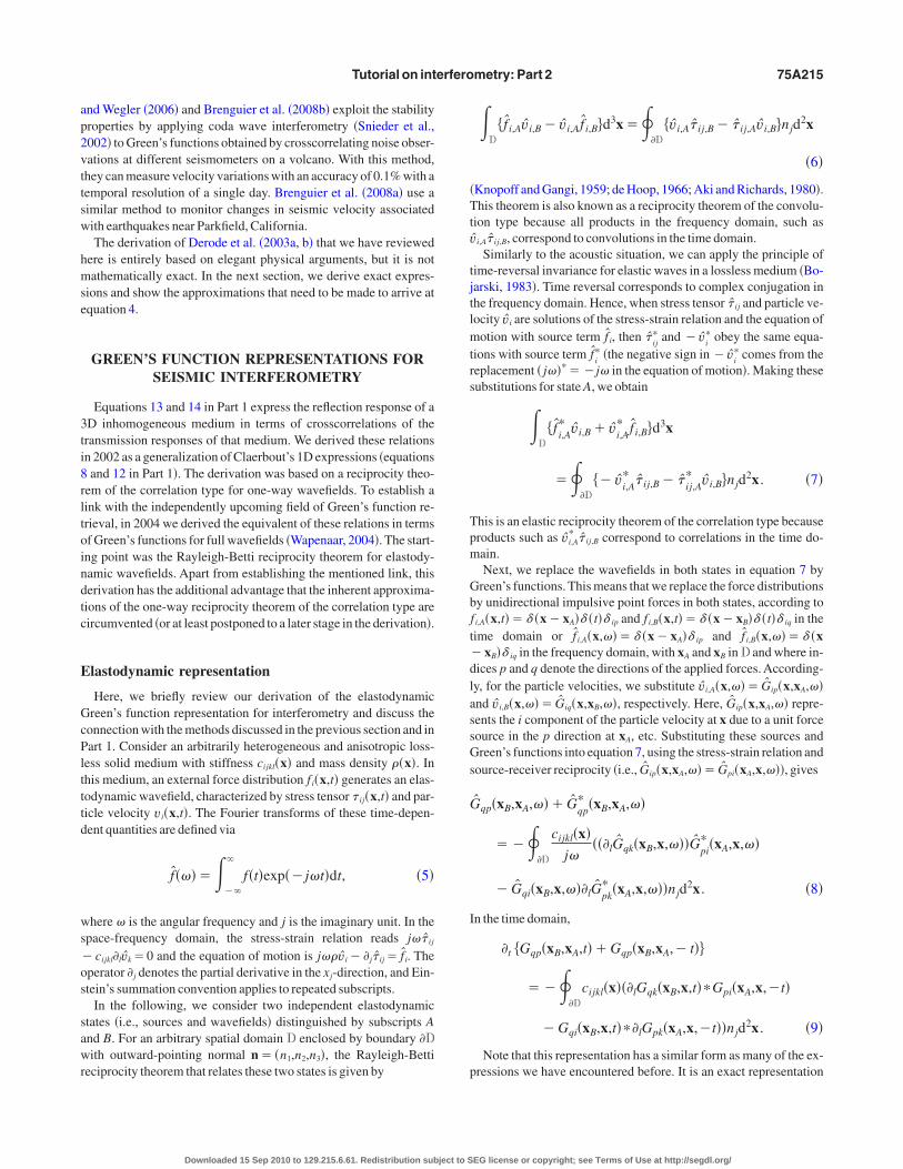
lastodynamic representation

Here, we briefly review our derivation of the elastodynamicreen’s function representation for interferometry and discuss the

onnection with the methods discussed in the previous section and inart 1. Consider an arbitrarily heterogeneous and anisotropic loss-

ess solid medium with stiffness cijkl�x� and mass density ��x�. Inhis medium, an external force distribution f i�x,t� generates an elas-odynamic wavefield, characterized by stress tensor � ij�x,t� and par-icle velocity vi�x,t�. The Fourier transforms of these time-depen-ent quantities are defined via

f��

�

f�t�exp��j�t�dt, �5�

here � is the angular frequency and j is the imaginary unit. In thepace-frequency domain, the stress-strain relation reads j�� ij

cijkl�lvk�0 and the equation of motion is j��vi��j� ij� f i. Theperator �j denotes the partial derivative in the xj-direction, and Ein-tein’s summation convention applies to repeated subscripts.

In the following, we consider two independent elastodynamictates �i.e., sources and wavefields� distinguished by subscripts And B. For an arbitrary spatial domain D enclosed by boundary �Dith outward-pointing normal n� �n1,n2,n3�, the Rayleigh-Betti

eciprocity theorem that relates these two states is given by


�D

� f i,Avi,B� vi,Af i,Bd3x��D

�vi,A� ij,B� � ij,Avi,Bnjd2x

�6�

Knopoff and Gangi, 1959; de Hoop, 1966; Aki and Richards, 1980�.his theorem is also known as a reciprocity theorem of the convolu-

ion type because all products in the frequency domain, such asˆ i,A� ij,B, correspond to convolutions in the time domain.

Similarly to the acoustic situation, we can apply the principle ofime-reversal invariance for elastic waves in a lossless medium �Bo-arski, 1983�. Time reversal corresponds to complex conjugation inhe frequency domain. Hence, when stress tensor � ij and particle ve-ocity vi are solutions of the stress-strain relation and the equation of

otion with source term f i, then �ij* and � v

i* obey the same equa-

ions with source term fi* �the negative sign in � v

i* comes from the

eplacement � j��*��j� in the equation of motion�. Making theseubstitutions for state A, we obtain

�D

� fi,A* vi,B� vi,A

* f i,Bd3x

��D

�� vi,A* � ij,B� �

ij,A* vi,Bnjd

2x . �7�

his is an elastic reciprocity theorem of the correlation type becauseroducts such as vi,A

* � ij,B correspond to correlations in the time do-ain.Next, we replace the wavefields in both states in equation 7 by

reen’s functions. This means that we replace the force distributionsy unidirectional impulsive point forces in both states, according to

f i,A�x,t�� x�xA�� t�� ip and f i,B�x,t�� x�xB�� t�� iq in theime domain or f i,A�x,�� x�xA�� ip and f i,B�x,�� x

xB�� iq in the frequency domain, with xA and xB in D and where in-ices p and q denote the directions of the applied forces. According-y, for the particle velocities, we substitute vi,A�x,�� Gip�x,xA,��nd vi,B�x,�� Giq�x,xB,��, respectively. Here, Gip�x,xA,�� repre-ents the i component of the particle velocity at x due to a unit forceource in the p direction at xA, etc. Substituting these sources andreen’s functions into equation 7, using the stress-strain relation and

ource-receiver reciprocity �i.e., Gip�x,xA,�� Gpi�xA,x,��, gives

ˆqp�xB,xA,�� G

qp* �xB,xA,��

��D

cijkl�x�j�

��lGqk�xB,x,��Gpi* �xA,x,��

� Gqi�xB,x,��lGpk* �xA,x,��njd

2x . �8�

n the time domain,

�t �Gqp�xB,xA,t��Gqp�xB,xA,� t�

��D

cijkl�x��lGqk�xB,x,t��Gpi�xA,x,�t�

�Gqi�xB,x,t��lGpk�xA,x,�t��njd2x . �9�

Note that this representation has a similar form as many of the ex-ressions we have encountered before. It is an exact representation


fvvfatbtbmoife

hww�cadfsstamcvsv

scdaa

hhampGtuBcso

wctlttrdfo

sstt2fistslfama4toaapboHs

�toc1

FapI�bmasG


or the Green’s function between xA and xB plus its time-reversedersion, expressed in terms of crosscorrelations of wavefield obser-ations at xA and xB, integrated along the sources at x on �D. It holdsor an arbitrarily inhomogeneous anisotropic medium �inside as wells outside �D�, and the closed boundary �D containing the sources ofhe Green’s functions may have any shape. When a part �D0 of theoundary is a stress-free surface, as in Figure 4, then the integrand ofhe right-hand side of equation 7 is zero on �D0. Consequently, theoundary integral in equation 9 need only be evaluated over the re-aining part �D1 �meaning that sources can be restricted to that part

f the boundary�. Note that equation 9 still holds in the limiting casen which xA and xB lie at the free surface. In that case, the Green’sunctions on the left-hand side have a traction source at xA �Wap-naar and Fokkema, 2006�.

An important difference with earlier expressions is that the right-and side of representation 9 contains a combination of two terms,here each of the terms is a crosscorrelation of Green’s functionsith different types of sources at x �e.g., the operator �l in

lGqk�xB,x,t� is a differentiation with respect to xl, which changes theharacter of the source at x of this Green’s function�. For modelingpplications, this is not a problem because any type of source can beefined in modeling. Van Manen et al. �2006, 2007� use equation 9or what they call interferometric modeling. They model the re-ponse of different types of sources on a boundary and save the re-ponses for all possible receiver positions in the volume enclosed byhe boundary. Next, they apply equation 9 to obtain the responses ofll possible source positions in that volume. Hence, for the cost ofodeling responses of sources on a boundary �and calculating many

rosscorrelations�, they obtain responses of sources throughout aolume. This approach can be very useful for nonlinear inversionchemes, where, in each iteration, Green’s functions for sources in aolume are required.

The requirement of correlating responses of different types ofources makes equation 9 in its present form less practical for appli-ation in seismic interferometry. This is particularly true for passiveata, where one must rely on the availability of natural sources. Toccommodate this situation, equation 9 can be modified �Wapenaarnd Fokkema, 2006�. Here, we only indicate the main steps. Using a

�D0

x�D1

xA xBGqp (xB ,xA , t )

igure 4. Configuration for elastodynamic Green’s function retriev-l �the rays represent the full response, including primary and multi-le scattering as well as mode conversion due to inhomogeneities�.n this configuration, a part of the closed boundary is a free surface�D0�, so sources are only required on the remaining part of theoundary ��D1�. The shallow sources �say, above the dashed line� areainly responsible for retrieving the surface waves and the direct

nd shallowly refracted waves in Gqp�xB,xA,t�, whereas the deeperources mainly contribute to the retrieval of the reflected waves in

�x ,x ,t�.
qp B A

igh-frequency approximation, assuming the medium outside �D isomogeneous and isotropic, the sources can be decomposed into P-nd S-wave sources and their derivatives in the direction of the nor-al on �D. These derivatives can be approximated, leading to a sim-

lified version of equation 9 in which only crosscorrelations ofreen’s functions with the same source type occur. This approxima-

ion is accurate when �D is a sphere with large radius. It can also besed for arbitrary surfaces �D but at the expense of amplitude errors.ecause the approximation does not affect the phase, it is usuallyonsidered acceptable for seismic interferometry. Finally, when theources are mutually uncorrelated noise sources for P- and S-wavesn �D, equation 9 reduces to

�Gqp�xB,xA,t��Gqp�xB,xA,�t��SN�t�

�2

�cPvq�xB,t��vp�xA,�t��, �10�

here vp�xA,t� and vq�xB,t� are the p and q components of the parti-le velocity of the noise responses at xA and xB, respectively; SN�t� ishe autocorrelation of the noise; and cP is the P-wave propagation ve-ocity of the homogeneous medium outside �D. For the configura-ion of Figure 4, the Green’s function Gqp�xB,xA,t� retrieved by equa-ion 10 contains the surface waves between xA and xB as well as theeflected and refracted waves, assuming the noise sources are wellistributed over the source boundary �D1 in the half-space below theree surface. In practice, equation 10 is used either for surface-waver for reflected-wave interferometry.

For surface-wave interferometry, the sources at and close to theurface typically give the most relevant contributions — say, theources above the dashed line in Figure 4. In our earlier, more intui-ive discussions on direct-wave interferometry in Part 1, we considerhe fundamental surface-wave mode as an approximate solution of aD wave equation in the horizontal plane and argue that the Green’sunction of this fundamental mode can be extracted by crosscorrelat-ng ambient noise. Equation 10 is a corollary of the exact 3D repre-entation 9 and thus accounts not only for the fundamental mode ofhe direct surface wave but also for higher-order modes as well as forcattered surface waves. Halliday and Curtis �2008� carefully ana-yze the contributions of the different sources to the retrieval of sur-ace waves. They show that when only sources at the surface arevailable, there is strong spurious interference between higherodes and the fundamental mode, whereas the presence of sources

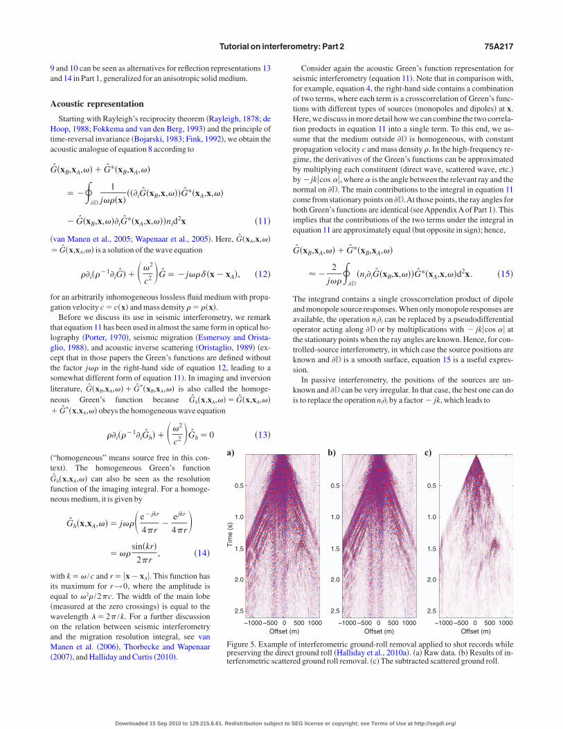
t depth �between the free surface and, say, the dashed line in Figure� enables the correct recovery of all modes independently. Never-heless, they show that it is possible to obtain the latter result usingnly surface sources if modes are separated before crosscorrelation,re correlated separately, and are reassembled thereafter. Kimmannd Trampert �2010� show that the spurious interference is also sup-ressed when the surface sources are very far away or organized in aand. Halliday and Curtis �2009b� analyze the requirements in termsf source distribution for the retrieval of scattered surface waves.alliday et al. �2010a� use the acquired insights to remove scattered

urface waves �ground roll� from seismic shot records �Figure 5�.For reflected-wave interferometry, the deeper situated sources

typically those below the dashed line in Figure 4� give the main con-ributions. This is in agreement with our discussion on the retrievalf the 3D reflection response from transmission data, for which weonsider a configuration with sources in the lower half-space �Figure2, Part 1�. For this configuration, Green’s function representations


9a

A

Hta

G

�

�

fg

tlgctsln�

�tGfn

wie�woaM�

sfotHtspgbbncbie

G

Taaottks

ki


and 10 can be seen as alternatives for reflection representations 13nd 14 in Part 1, generalized for an anisotropic solid medium.

coustic representation

Starting with Rayleigh’s reciprocity theorem �Rayleigh, 1878; deoop, 1988; Fokkema and van den Berg, 1993� and the principle of

ime-reversal invariance �Bojarski, 1983; Fink, 1992�, we obtain thecoustic analogue of equation 8 according to

ˆ �xB,xA,�� G*�xB,xA,��

��D

1

j��x��iG�xB,x,��G*�xA,x,��

� G�xB,x,��iG*�xA,x,��nid2x �11�

van Manen et al., 2005; Wapenaar et al., 2005�. Here, G�xA,x,��G�x,xA,�� is a solution of the wave equation

��i��1�iG��2

c2 G��j�� x�xA�, �12�

or an arbitrarily inhomogeneous lossless fluid medium with propa-ation velocity c�c�x� and mass density � ��x�.Before we discuss its use in seismic interferometry, we remark

hat equation 11 has been used in almost the same form in optical ho-ography �Porter, 1970�, seismic migration �Esmersoy and Orista-lio, 1988�, and acoustic inverse scattering �Oristaglio, 1989� �ex-ept that in those papers the Green’s functions are defined withouthe factor j�� in the right-hand side of equation 12, leading to aomewhat different form of equation 11�. In imaging and inversioniterature, G�xB,xA,�� G*�xB,xA,�� is also called the homoge-eous Green’s function because Gh�x,xA,�� G�x,xA,��

G*�x,xA,�� obeys the homogeneous wave equation

��i��1�iGh��2

c2 Gh�0 �13�

“homogeneous” means source free in this con-ext�. The homogeneous Green’s functionˆ

h�x,xA,�� can also be seen as the resolutionunction of the imaging integral. For a homoge-eous medium, it is given by

Gh�x,xA,�� j�� e�jkr

4�r�

e jkr

4�r

��sin�kr�

2�r, �14�

ith k�� /c and r� �x�xA�. This function hasts maximum for r→0, where the amplitude isqual to �2� /2�c. The width of the main lobemeasured at the zero crossings� is equal to theavelength �2� /k. For a further discussionn the relation between seismic interferometrynd the migration resolution integral, see vananen et al. �2006�, Thorbecke and Wapenaar

2007�, and Halliday and Curtis �2010�.

0.5

1.0

1.5

2.0

2.5

–1000 –50O

Tim

e(s

)

a)

Figure 5. Exapreserving theterferometric


Consider again the acoustic Green’s function representation foreismic interferometry �equation 11�. Note that in comparison with,or example, equation 4, the right-hand side contains a combinationf two terms, where each term is a crosscorrelation of Green’s func-ions with different types of sources �monopoles and dipoles� at x.ere, we discuss in more detail how we can combine the two correla-

ion products in equation 11 into a single term. To this end, we as-ume that the medium outside �D is homogeneous, with constantropagation velocity c and mass density �. In the high-frequency re-ime, the derivatives of the Green’s functions can be approximatedy multiplying each constituent �direct wave, scattered wave, etc.�y �jk�cos �, where is the angle between the relevant ray and theormal on �D. The main contributions to the integral in equation 11ome from stationary points on �D.At those points, the ray angles foroth Green’s functions are identical �see Appendix A of Part 1�. Thismplies that the contributions of the two terms under the integral inquation 11 are approximately equal �but opposite in sign�; hence,


��2

j��

�D�ni�iG�xB,x,��G*�xA,x,��d2x . �15�

he integrand contains a single crosscorrelation product of dipolend monopole source responses. When only monopole responses arevailable, the operation ni�i can be replaced by a pseudodifferentialperator acting along �D or by multiplications with � jk�cos � athe stationary points when the ray angles are known. Hence, for con-rolled-source interferometry, in which case the source positions arenown and �D is a smooth surface, equation 15 is a useful expres-ion.

In passive interferometry, the positions of the sources are un-nown and �D can be very irregular. In that case, the best one can dos to replace the operation ni�i by a factor � jk, which leads to

500 1000)

0.5

1.0

1.5

2.0

2.5

–1000 –500 0 500 1000Offset (m)

0.5

1.0

1.5

2.0

2.5

–1000 –500 0 500 1000Offset (m)

b) c)

f interferometric ground-roll removal applied to shot records whileground roll �Halliday et al., 2010a�. �a� Raw data. �b� Results of in-d ground roll removal. �c� The subtracted scattered ground roll.

0 0ffset (m

mple odirect

scattere


G

Tstsbpeo

G

we

almtRsweiw

coFihasc

fioiwsaa�tra

C

�

R1tt

jfitofieisg�df

tecbetetob�pt

f

M

gtMrishrS

v�alaf



�2

�c�

�DG�xB,x,��G*�xA,x,��d2x . �16�

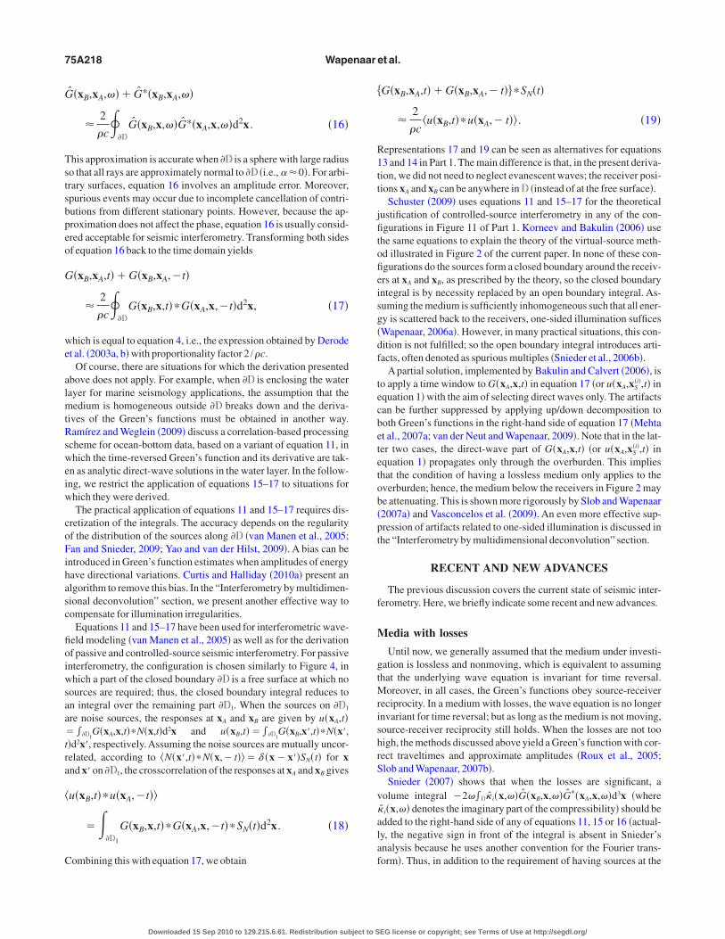
his approximation is accurate when �D is a sphere with large radiuso that all rays are approximately normal to �D �i.e., �0�. For arbi-rary surfaces, equation 16 involves an amplitude error. Moreover,purious events may occur due to incomplete cancellation of contri-utions from different stationary points. However, because the ap-roximation does not affect the phase, equation 16 is usually consid-red acceptable for seismic interferometry. Transforming both sidesf equation 16 back to the time domain yields

�xB,xA,t��G�xB,xA,�t�

�2

�c�

�DG�xB,x,t��G�xA,x,�t�d2x, �17�

hich is equal to equation 4, i.e., the expression obtained by Derodet al. �2003a, b� with proportionality factor 2 /�c.

Of course, there are situations for which the derivation presentedbove does not apply. For example, when �D is enclosing the waterayer for marine seismology applications, the assumption that the

edium is homogeneous outside �D breaks down and the deriva-ives of the Green’s functions must be obtained in another way.amírez and Weglein �2009� discuss a correlation-based processing

cheme for ocean-bottom data, based on a variant of equation 11, inhich the time-reversed Green’s function and its derivative are tak-

n as analytic direct-wave solutions in the water layer. In the follow-ng, we restrict the application of equations 15–17 to situations forhich they were derived.The practical application of equations 11 and 15–17 requires dis-

retization of the integrals. The accuracy depends on the regularityf the distribution of the sources along �D �van Manen et al., 2005;an and Snieder, 2009; Yao and van der Hilst, 2009�. A bias can be

ntroduced in Green’s function estimates when amplitudes of energyave directional variations. Curtis and Halliday �2010a� present anlgorithm to remove this bias. In the “Interferometry by multidimen-ional deconvolution” section, we present another effective way toompensate for illumination irregularities.

Equations 11 and 15–17 have been used for interferometric wave-eld modeling �van Manen et al., 2005� as well as for the derivationf passive and controlled-source seismic interferometry. For passiventerferometry, the configuration is chosen similarly to Figure 4, inhich a part of the closed boundary �D is a free surface at which no

ources are required; thus, the closed boundary integral reduces ton integral over the remaining part �D1. When the sources on �D1

re noise sources, the responses at xA and xB are given by u�xA,t��D1

G�xA,x,t��N�x,t�d2x and u�xB,t��D1G�xB,x�,t��N�x�,

�d2x�, respectively. Assuming the noise sources are mutually uncor-elated, according to N�x�,t��N�x,�t�� x�x��SN�t� for xnd x� on �D1, the crosscorrelation of the responses at xA and xB gives

u�xB,t��u�xA,�t��

��D1

G�xB,x,t��G�xA,x,�t��SN�t�d2x . �18�

ombining this with equation 17, we obtain


G�xB,xA,t��G�xB,xA,� t��SN�t�

�2

�cu�xB,t��u�xA,� t�� . �19�

epresentations 17 and 19 can be seen as alternatives for equations3 and 14 in Part 1. The main difference is that, in the present deriva-ion, we did not need to neglect evanescent waves; the receiver posi-ions xA and xB can be anywhere in D �instead of at the free surface�.

Schuster �2009� uses equations 11 and 15–17 for the theoreticalustification of controlled-source interferometry in any of the con-gurations in Figure 11 of Part 1. Korneev and Bakulin �2006� use

he same equations to explain the theory of the virtual-source meth-d illustrated in Figure 2 of the current paper. In none of these con-gurations do the sources form a closed boundary around the receiv-rs at xA and xB, as prescribed by the theory, so the closed boundaryntegral is by necessity replaced by an open boundary integral. As-uming the medium is sufficiently inhomogeneous such that all ener-y is scattered back to the receivers, one-sided illumination sufficesWapenaar, 2006a�. However, in many practical situations, this con-ition is not fulfilled; so the open boundary integral introduces arti-acts, often denoted as spurious multiples �Snieder et al., 2006b�.

Apartial solution, implemented by Bakulin and Calvert �2006�, iso apply a time window to G�xA,x,t� in equation 17 �or u�xA,xS

�i�,t� inquation 1� with the aim of selecting direct waves only. The artifactsan be further suppressed by applying up/down decomposition tooth Green’s functions in the right-hand side of equation 17 �Mehtat al., 2007a; van der Neut and Wapenaar, 2009�. Note that in the lat-er two cases, the direct-wave part of G�xA,x,t� �or u�xA,xS

�i�,t� inquation 1� propagates only through the overburden. This implieshat the condition of having a lossless medium only applies to theverburden; hence, the medium below the receivers in Figure 2 maye attenuating. This is shown more rigorously by Slob and Wapenaar2007a� and Vasconcelos et al. �2009�. An even more effective sup-ression of artifacts related to one-sided illumination is discussed inhe “Interferometry by multidimensional deconvolution” section.

RECENT AND NEW ADVANCES

The previous discussion covers the current state of seismic inter-erometry. Here, we briefly indicate some recent and new advances.

edia with losses

Until now, we generally assumed that the medium under investi-ation is lossless and nonmoving, which is equivalent to assuminghat the underlying wave equation is invariant for time reversal.

oreover, in all cases, the Green’s functions obey source-receivereciprocity. In a medium with losses, the wave equation is no longernvariant for time reversal; but as long as the medium is not moving,ource-receiver reciprocity still holds. When the losses are not tooigh, the methods discussed above yield a Green’s function with cor-ect traveltimes and approximate amplitudes �Roux et al., 2005;lob and Wapenaar, 2007b�.Snieder �2007� shows that when the losses are significant, a

olume integral �2��D� i�x,��G�xB,x,��G*�xA,x,��d3x �whereˆ i�x,�� denotes the imaginary part of the compressibility� should bedded to the right-hand side of any of equations 11, 15 or 16 �actual-y, the negative sign in front of the integral is absent in Snieder’snalysis because he uses another convention for the Fourier trans-orm�. Thus, in addition to the requirement of having sources at the


boeifba�

vHlafdt

N

vsi1Gmmshadrmms

a2cmiosi

U

c

woufmu�c

Wipe

wtfiaanmtlu

�tt

Nf�tfioGsal

Fmrxwwgp


oundary �D �as in Figures 3c and 4�, sources are required through-ut the domain D. When these sources are uncorrelated noise sourc-s, the final expression for Green’s function retrieval again has a sim-lar form as equation 19. This volume integral approach to Green’sunction retrieval is not restricted to acoustic waves in lossy mediaut also applies to electromagnetic waves in conductive media �Slobnd Wapenaar, 2007a� as well as to pure diffusion phenomenaSnieder, 2006�.

In most practical situations, sources are not available throughout aolume. Interferometry by crossconvolution �Slob et al., 2007a;alliday and Curtis, 2009b� is another approach that accounts for

osses. Draganov et al. �2010� compensate for losses with an inversettenuation filter. By doing this adaptively �aiming to minimize arti-acts�, they estimate the attenuation parameters. The methodologyiscussed in the “Interferometry by multidimensional deconvolu-ion” section also accounts very effectively for losses.

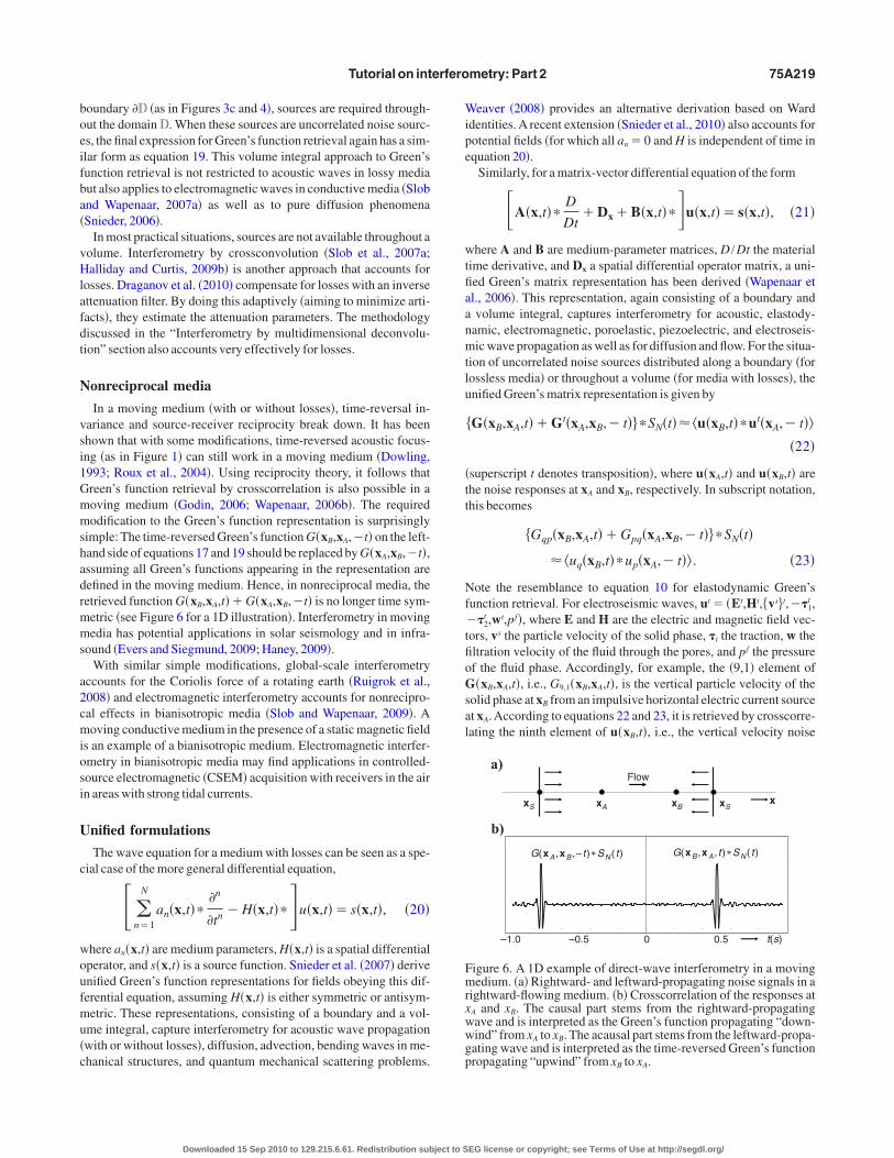
onreciprocal media

In a moving medium �with or without losses�, time-reversal in-ariance and source-receiver reciprocity break down. It has beenhown that with some modifications, time-reversed acoustic focus-ng �as in Figure 1� can still work in a moving medium �Dowling,993; Roux et al., 2004�. Using reciprocity theory, it follows thatreen’s function retrieval by crosscorrelation is also possible in aoving medium �Godin, 2006; Wapenaar, 2006b�. The requiredodification to the Green’s function representation is surprisingly

imple: The time-reversed Green’s function G�xB,xA,�t� on the left-and side of equations 17 and 19 should be replaced by G�xA,xB,�t�,ssuming all Green’s functions appearing in the representation areefined in the moving medium. Hence, in nonreciprocal media, theetrieved function G�xB,xA,t��G�xA,xB,�t� is no longer time sym-etric �see Figure 6 for a 1D illustration�. Interferometry in movingedia has potential applications in solar seismology and in infra-

ound �Evers and Siegmund, 2009; Haney, 2009�.With similar simple modifications, global-scale interferometry

ccounts for the Coriolis force of a rotating earth �Ruigrok et al.,008� and electromagnetic interferometry accounts for nonrecipro-al effects in bianisotropic media �Slob and Wapenaar, 2009�. Aoving conductive medium in the presence of a static magnetic field

s an example of a bianisotropic medium. Electromagnetic interfer-metry in bianisotropic media may find applications in controlled-ource electromagnetic �CSEM� acquisition with receivers in the airn areas with strong tidal currents.

nified formulations

The wave equation for a medium with losses can be seen as a spe-ial case of the more general differential equation,

� �n�1

N

an�x,t��n

�tn �H�x,t��u�x,t��s�x,t�, �20�

here an�x,t� are medium parameters, H�x,t� is a spatial differentialperator, and s�x,t� is a source function. Snieder et al. �2007� derivenified Green’s function representations for fields obeying this dif-erential equation, assuming H�x,t� is either symmetric or antisym-etric. These representations, consisting of a boundary and a vol-

me integral, capture interferometry for acoustic wave propagationwith or without losses�, diffusion, advection, bending waves in me-hanical structures, and quantum mechanical scattering problems.


eaver �2008� provides an alternative derivation based on Warddentities. A recent extension �Snieder et al., 2010� also accounts forotential fields �for which all an�0 and H is independent of time inquation 20�.

Similarly, for a matrix-vector differential equation of the form

�A�x,t��D

Dt�Dx�B�x,t��u�x,t��s�x,t�, �21�

here A and B are medium-parameter matrices, D /Dt the materialime derivative, and Dx a spatial differential operator matrix, a uni-ed Green’s matrix representation has been derived �Wapenaar etl., 2006�. This representation, again consisting of a boundary andvolume integral, captures interferometry for acoustic, elastody-

amic, electromagnetic, poroelastic, piezoelectric, and electroseis-ic wave propagation as well as for diffusion and flow. For the situa-

ion of uncorrelated noise sources distributed along a boundary �forossless media� or throughout a volume �for media with losses�, thenified Green’s matrix representation is given by

�G�xB,xA,t��Gt�xA,xB,� t��SN�t��u�xB,t��ut�xA,� t��

�22�

superscript t denotes transposition�, where u�xA,t� and u�xB,t� arehe noise responses at xA and xB, respectively. In subscript notation,his becomes

�Gqp�xB,xA,t��Gpq�xA,xB,� t��SN�t�

�uq�xB,t��up�xA,� t�� . �23�

ote the resemblance to equation 10 for elastodynamic Green’sunction retrieval. For electroseismic waves, ut� �Et,Ht,�vst,��1

t ,�2

t ,wt,pf�, where E and H are the electric and magnetic field vec-ors, vs the particle velocity of the solid phase, �i the traction, w theltration velocity of the fluid through the pores, and pf the pressuref the fluid phase. Accordingly, for example, the �9,1� element of�xB,xA,t�, i.e., G9,1�xB,xA,t�, is the vertical particle velocity of the

olid phase at xB from an impulsive horizontal electric current sourcet xA.According to equations 22 and 23, it is retrieved by crosscorre-ating the ninth element of u�xB,t�, i.e., the vertical velocity noise

−1 −0.8 −0.6 −0.4 −0.2 0 0.2 0.4 0.6 0.8 1−10

−5

0

5

10

15

20

Flow

–1.0 –0.5 0 0.5 t(s)

xS xA xB xSx

G(xA ,xB ,– t )�SN ( t ) G(xB ,xA , t )�SN ( t )

a)

b)

igure 6. A 1D example of direct-wave interferometry in a movingedium. �a� Rightward- and leftward-propagating noise signals in a

ightward-flowing medium. �b� Crosscorrelation of the responses atA and xB. The causal part stems from the rightward-propagatingave and is interpreted as the Green’s function propagating “down-ind” from xA to xB. The acausal part stems from the leftward-propa-ating wave and is interpreted as the time-reversed Green’s functionropagating “upwind” from x to x .
B A

fittR

R

CscN

wot

tlrptifshIatom

V

tsae

icTrAvpspisd

2mtttccorla

�btaTwsficsoi

swfcai

Ftsvcop

Fsa


eld at xB with the first element of u�xA,t� being the horizontal elec-ric noise field at xA �Figure 7�. For a further discussion on elec-roseismic interferometry, including numerical examples, see deidder et al. �2009�.

elation with the generalized optical theorem

It has recently been recognized �Snieder et al., 2008; Halliday andurtis, 2009a� that the frequency-domain Green’s function repre-

entation for seismic interferometry resembles the generalized opti-al theorem �Heisenberg, 1943; Glauber and Schomaker, 1953;ewton, 1976; Marston, 2001�, given by

�1

2j�f�kA,kB�� f *�kB,kA��

k

4�� f�k,kB�f *�k,kA�d� ,

�24�

here f�kA,kB� is the far-field angle-dependent scattering amplitudef a finite scatterer �Figure 8�, including all linear and nonlinear in-eractions of the wavefield with the scatterer.

The optical theorem has a form similar to interferometry represen-ation 16 for acoustic waves. The analysis of this resemblance hased to new insights in interferometry as well as in scattering theo-ems. Snieder et al. �2008� use the generalized optical theorem to ex-lain the cancellation of specific spurious arrivals in Green’s func-ion extraction. Halliday and Curtis �2009a� show that the general-zed optical theorem can be derived from the interferometric Green’sunction representation and use this to derive an optical theorem forurface waves in layered elastic media. Snieder et al. �2009b� discussow the scattering amplitude can be derived from field fluctuations.n other related work, Halliday and Curtis �2009b� and Wapenaar etl. �2010� show that the Born approximation is an insufficient modelo explain all aspects of seismic interferometry, even for the situationf a single point scatterer, and use this insight to derive improvedodels for the scattering amplitude of a point scatterer.

irtual receivers, reflectors, and imaging

Until now, we have discussed seismic interferometry as a methodhat retrieves the response of a virtual source by crosscorrelating re-ponses at two receivers. Using reciprocity, it is also possible to cre-te a virtual receiver by crosscorrelating the responses of two sourc-s. Curtis et al. �2009� use this principle to turn earthquake sources

3svE1

Controlled transient sources

Uncorrelated noise sources

1e

J 3sv

G9,1(xB ,xA , t )

igure 7. Principle of electroseismic interferometry for controlledransient sources at the surface or uncorrelated noise sources in theubsurface. In this example, the vertical component of the particleelocity of the solid phase is crosscorrelated with the horizontalomponent of the electric field, yielding the electroseismic responsef a horizontal electric current source observed by a vertical geo-hone.


nto virtual seismometers with which real seismograms can be re-orded, located noninvasively deep within the earth’s subsurface.hey argue that this methodology has the potential to improve the

esolution of imaging the earth’s interior by earthquake seismology.n earthquake source acts like a double couple; so by reciprocity, theirtual receiver acts like a strainmeter, a device that is not easily im-lemented by a physical instrument. In a similar way, microseismicources near a reservoir could be turned into virtual receivers to im-rove the resolution of reservoir imaging �Figure 9�. Note that imag-ng using virtual receivers requires knowledge of the position of theources, but recording seismograms on the virtual seismometersoes not.

Another variant is the virtual reflector method �Poletto and Farina,008; Poletto and Wapenaar, 2009�. This method creates new seis-ic signals by processing real seismic responses of impulsive or

ransient sources. Under proper recording coverage conditions, thisechnique obtains seismograms as if there were an ideal reflector athe position of the receivers �or sources�. The algorithm consists ofonvolution of the recorded traces, followed by integration of therossconvolved signals along the receivers �or sources�. Similar tother interferometry methods, the virtual reflector method does notequire information on the propagation velocity of the medium. Po-etto and Farina �2010� illustrate the method with synthetic marinend real borehole data.

Curtis �2009�, Schuster �2009, chapter 8�, and Curtis and Halliday2010b� discuss source-receiver interferometry. This method com-ines the virtual-source and the virtual-receiver methodologies andhus involves a double integration over sources and receivers. It cre-tes the response of a virtual source observed by a virtual receiver.his method is related to prestack redatuming �Berryhill, 1984�, inhich sources and receivers are repositioned from the acquisition

urface to a new datum plane in the subsurface, using one-way wave-eld extrapolation operators based on a macromodel. In source-re-eiver interferometry, the operators are replaced by measured re-ponses — for example, in VSPs. Hence, source-receiver interfer-metry can be seen as the data-driven variant of prestack redatum-ng.

Note, however, that in general the measured responses used inource-receiver interferometry are full wavefields rather than one-ay operators. Therefore, the application of source-receiver inter-

erometry is not restricted to data-driven prestack redatuming, but itan be used for other applications as well. For example, Halliday etl. �2010b� show that the elastodynamic version of source-receivernterferometry can be seen as a generalization of a method that turns

kB kA

igure 8. The generalized optical theorem for the angle-dependentcattering amplitude f�kA,kB� �Heisenberg, 1943� has a similar forms the Green’s function representation for seismic interferometry.


PvicAtrmPptHnml

i�lwtr

T

mhcB�ap2scsrfipettt2

�sfopsu

ssc

G

w2wtigtrts

I

Grc

Attwtfsuudd

Fmoslsf


Pand PS data into SS data, previously proposed by Grechka and Ts-ankin �2002� and Grechka and Dewangan �2003�. In a similar fash-on, the internal multiple prediction method of Jakubowicz �1998�an be derived as a special case of source-receiver interferometry.lso, the surface-wave-removal methods of Dong et al. �2006�, Cur-

is et al. �2006�, and Halliday et al. �2007, 2010a� require physicallyecorded and interferometrically constructed Green’s function esti-ates between the locations of an active source and active receiver.reviously, the interferometric estimate was obtained by having tolace a receiver beside every source and turning the former into a vir-ual source �or vice versa, using virtual-receiver interferometry�.owever, by using source-receiver interferometry, this becomes un-ecessary because the interferometric wavefield estimate can beade between real source and real receiver directly �Curtis and Hal-

iday, 2010b�.Similar double integrals appear in the acoustic inverse scattering

maging formulation of Oristaglio �1989�. Halliday and Curtis2010� derive explicitly a generalized version of Oristaglio’s formu-ation from a version of source-receiver interferometry for a mediumith scattering perturbations. The derivation was possible because

his form of interferometry is the first to combine active sources andeceivers, similar to geometries used for imaging.

ime-lapse seismic interferometry

As a consequence of the stability of time-reversed acoustics, seis-ic interferometry has large potential for time-lapse methods. We

ave indicated the use of passive interferometry for monitoringhanges in volcanic interiors �Sens-Schönfelder and Wegler, 2006;renguier et al., 2008b�. Using the same principles, Brenguier et al.

2008a� monitor postseismic relaxation along the San Andreas faultt Parkfield, California, U.S.A., and Ohmi et al. �2008� monitor tem-oral variations of the crustal structure in the source region of the007 Noto Hanto earhquake in central Japan. Kraeva et al. �2009�how a relation between seasonal variations of ambient noise cross-orrelations and remote microseismic activity related to oceantorms, and Haney �2009� reports on time-dependent effects in cor-elations of infrasound that arise from time-varying temperatureelds and temperature inversion layers in the atmosphere. The inter-retation in all these methods is based on measuring the time shift inither the direct wave or the coda wave of the Green’s functions re-rieved by interferometry. These time shifts give information abouthe average velocity change between the receivers, which can be fur-her regionalized by tomographic inversion �Brenguier et al.,008b�.

In the field of controlled-source interferometry, Bakulin et al.2007� and Mehta et al. �2008� discuss the potential of the virtual-ource method for time-lapse reservoir monitoring. They exploit theact that virtual-source data are obtained from permanent downholer ocean-bottom-cable receivers and hence have a high degree of re-eatability. Because virtual-source data represent reflection re-ponses, local time-lapse changes in these data can be reliably attrib-ted to local changes in the reservoir.

To better quantify the time-lapse changes in the data obtained byeismic interferometry, the interferometric Green’s function repre-entation �equation 11� has been modified to account for time-lapsehanges according to



��D

1

j��x��iG�xB,x,��G*�xA,x,��

� G�xB,x,��iG*�xA,x,��nid2x

� j��D

��x,��G�xB,x,��G*�xA,x,��d3x, �25�

ith ��x,�� x,�� *�x,�� Vasconcelos and Snieder,008a; Douma, 2009; Vasconcelos et al., 2009�. Here, the quantitiesith/without a bar refer to the reference/monitor state �for simplici-

y, we assume that time-lapse changes occur only in the compress-bility�. The equivalent theory for source-receiver interferometry isiven in Halliday and Curtis �2010�. Equation 25 and its generaliza-ion for other wave types �Wapenaar, 2007� provides a basis for de-iving local time-lapse changes of the medium parameters from in-erferometric time-lapse data. This is the subject of ongoing re-earch.

nterferometry by deconvolution and crosscoherence

In the previous treatment of interferometry, we focused onreen’s function extraction by crosscorrelation. Time reversal cor-

esponds to complex conjugation in the frequency domain, so therosscorrelation is, in the frequency domain, given by

C�xB,xA,�� u�xB,��u*�xA,�� . �26�

ccording to expression 19, the crosscorrelation does not just givehe superposition of the Green’s function and its time-reversed coun-erpart because the left-hand side of that expression is convolvedith the autocorrelation of the noise that excites the field fluctua-

ions. This means that equation 26 gives the product of the Green’sunction and the power spectrum SN�� of the noise. The powerpectrum thus leaves an imprint on the extracted Green’s functionnless it is properly accounted for. This imprint can be eliminated bysing deconvolution instead of crosscorrelation. In the frequencyomain, deconvolution corresponds to spectral division; hence, theeconvolution approach consists of replacing expression 26 by

x

Complexoverburden

Simplermiddleoverburden

Target

u (x ,xA , t )

xB

u (x ,xB , t )

x A (Virtual receiver)

G (xA ,x t )B ,

igure 9. Using reciprocity, Bakulin and Calvert’s virtual-sourceethod �Figure 2� can be reformulated into a virtual receiver meth-

d. Receivers at the surface record the direct and the reflection re-ponses of microseismic sources above a deeper target. Crosscorre-ation and summing over receiver locations gives the reflection re-ponse at a virtual receiver at the position of a microseismic source,ree of overburden distortions.


Wot

wda

tlbTtsd

Ferhp

wxi2pesw

n

T

DvthtT

c

tprr�

ctg

wpdtl

wwat2cSel2

opc�od

wmAsamg

Trah�amt


D�xB,xA,��u�xB,��u�xA,��

. �27�

hen u�xA,�� is small, this spectral division is unstable. In practice,ne needs to regularize the deconvolution. The simplest way to dohis is to use the following water-level regularization:

D�xB,xA,��u�xB,��u*�xA,��u�xA,��2��2 , �28�

here �2 is a stabilization parameter. When �2�0, expression 28 re-uces to equation 27; for �2� � u�xA,��2, equation 28 corresponds toscaled version of the correlation defined in expression 26.A significant difference between crosscorrelation and deconvolu-

ion is that crosscorrelation gives the Green’s function but deconvo-ution does not. This raises the question, what wave state is retrievedy deconvolving field measurements recorded at different points?here is a simple proof that the wave states obtained by crosscorrela-

ion, deconvolution, and regularized deconvolution all satisfy theame equation as the real system does �Snieder et al., 2006a�. Let usenote the field equation of the system by

L�x,��u�x,��0. �29�

or the acoustic wave equation in a constant-density medium, forxample, the operator L is given by L�x,��2��2 /c2�x�. Theight-hand side of expression 29 equals zero, so this expressionolds for source-free regions, which is the case at the receivers. Ap-lying L to equation 27 with xB replaced by x gives

L�x,��D�x,xA,�� L�x,�� u�x,��u�xA,��

�

1

u�xA,��L�x,��u�x,��0, �30�

here in the second identity we used that L�x,�� acts on the-coordinates only and where the field equation 29 is used in the lastdentity. The same reasoning applies to the correlation of expression6 and the regularized deconvolution in expression 28. All of theserocedures thus produce a wave state that satisfies the same wavequation as the original system does. For the correlation, this wavetate is the Green’s function; but for the deconvolution, a differentave state is obtained.To understand which wave state is extracted by deconvolution, we

ote that

D�xA,xA,��u�xA,��u�xA,��

�1. �31�

his corresponds, in the time domain, to

D�xA,xA,t�� t� . �32�

econvolution thus gives a wave state that, for t�0, vanishes at theirtual-source location xA. This means that the wavefield vanishes athat location, and hence, the phrase “clamped boundary condition”as been used �Vasconcelos and Snieder, 2008a�. Deconvolutionhus gives a wave state where the field vanishes at one point in space.his wave state is, in general, not equal to the Green’s function.Despite this strange boundary condition, interferometry by de-

onvolution has a distinct advantage for attenuating media. Consider


he example of Figure 1a of Part 1 of this tutorial where a plane waveropagates along a line from a source at xS to receivers at xA and xB,espectively. For a homogeneous attenuating medium, the fieldecorded at xA equals u�xA,�� G�xA,xS,��N��exp�� xA

xS��exp��jk�xA�xS��N��, where � is an attenuation coeffi-ient and N�� is the source spectrum.Asimilar expression holds forhe field at xB. The correlation of the fields recorded at xA and xB isiven by

C�xB,xA,��e�� xA�xB�2xS�e�jk�xB�xA�SN��, �33�

ith SN�� N��2. This field has the same phase as the field thatropagates from xA to xB, but the attenuation is incorrect because itepends on the source location xS, which is, of course, not related tohe field that propagates between xA and xB. In contrast, the deconvo-ution of the recorded fields satisfies

D�xB,xA,��e�� xB�xA�e�jk�xB�xA�� G�xB,xA,��,

�34�

hich does correctly account for the phase and the amplitude andhich does not depend on N��. This property of the deconvolution

pproach for 1D systems has been used to extract the velocity and at-enuation in the near surface �Trampert et al., 1993; Mehta et al.,007b� and to determine the structural response of buildings from in-oherent ground motion �Snieder and Şafak, 2006; Thompson andnieder, 2006; Kohler et al., 2007�. The deconvolution method hasven been used to detect changes in the near-surface shear-wave ve-ocity during shaking caused by an earthquake �Sawazaki et al.,009�.

The application of deconvolution interferometry changes whenne can separate the wavefield into an unperturbed wave u0 and aerturbation uS �Vasconcelos and Snieder, 2008b�. Such a separationan be achieved by time gating when impulsive shots are usedBakulin et al., 2007; Mehta et al., 2007a�, by using array methods,r by using four-component data. In this case, one can define a neweconvolution,

D��xB,xA,��uS�xB,��u0�xA,��

, �35�

hich gives an estimate of the perturbed Green’s function GS. Thisodified deconvolution method has been used to illuminate the Sanndreas fault from the side using drill-bit noise �Figure 10� and for

ubsalt imaging from below using internal multiples �Vasconcelos etl., 2008�. A comparison of crosscorrelation, deconvolution, andultidimensional deconvolution �presented in the next section� is

iven by Snieder et al. �2009a�.Amethod related to deconvolution is crosscoherence, defined as

H�xB,xA,��u�xB,��u�xB,��

u*�xA,��u�xA,��

. �36�

he crosscoherence can be seen as a spectrally normalized crosscor-elation or as a variant of deconvolution that is symmetric in u�xA,��nd u�xB,��. This method of combining data is proposed by Aki inis seminal papers on retrieving surface waves from microtremors1957, 1965�. It has been used extensively in engineering �Bendatnd Piersol, 2000� in the extraction of response functions and is com-only used to determine shallow shear velocity from ground vibra-

ions, e.g., Chávez-García and Luzón �2005�. Note that the reason-


icold

I

nd�scn

vt

witteGSpshbssn1

wts

wibont

cua

w

a

NttatwswtCcw

pemGtvsmsts

F�bifartep


ng leading to equation 30 is not applicable to the crosscoherence be-ause of the presence of the normalized spectrum in the denominatorf expression 36. Hence, the crosscoherence does not necessarilyead to a wave state that satisfies the same equation as the real systemoes.

nterferometry by multidimensional deconvolution

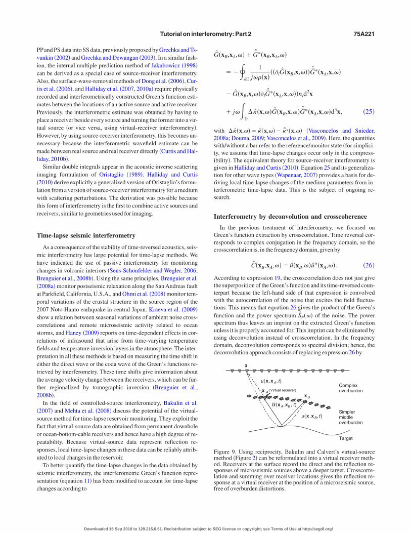
Interferometry by multidimensional deconvolution �MDD� is theatural extension of interferometry by deconvolution to two or threeimensions. It has been proposed for controlled-source dataSchuster and Zhou, 2006; Wapenaar et al., 2008a� as well as for pas-ive data �Wapenaar et al., 2008b�. Here, we discuss the principle forontrolled-source data and briefly indicate the modifications foroise data.

Consider again Figure 2, which we initially used to introduce theirtual-source method of Bakulin and Calvert �2004�. We expresshe upgoing wavefield at xB as

u��xB,xS�i�,t��G�xB,xA,t��u��xA,xS

�i�,t�dxA, �37�

here the plus and minus superscripts refer to downgoing and upgo-ng waves, respectively. Note that the integration takes place alonghe receivers at xA in the borehole. This convolutional data represen-ation is valid in media with or without losses. However, unlikequation 1, which is an explicit but approximate expression for thereen’s function G�xB,xA,t� �convolved with the autocorrelation

s�t� of the source wavelet�, equation 37 is an implicit but exact ex-ression for G�xB,xA,t� �with G�xB,xA,t� being the reflection re-ponse of the medium below the receiver level with a homogeneousalf-space above it �Wapenaar, Slob, et al., 2008��. Equation 37 cane solved by MDD, assuming responses are available for manyource positions xS

�i�. In that case, equation 37 holds for each sourceeparately. In the frequency domain, the resulting set of simulta-eous equations can be represented in matrix notation �Berkhout,982� according to

U��GU�, �38�

here the � j,i� element of U� is given by u��xA�j�,xS

�i�,��, etc. Equa-ion 38 can be solved for G, e.g., via weighted least-squares inver-ion �Menke, 1989�, according to

G� U�W�U�†�U�W�U�†��2I��1, �39�

here the dagger denotes transposition and complex conjugation, Ws a diagonal weighting matrix, I is the identity matrix, and �2 is a sta-ilization parameter. Equation 39 is the multidimensional extensionf equation 28. Applying this equation for each frequency compo-ent and transforming the result to the time domain accomplishes in-erferometry by MDD.

To get more insight into equation 37 and its solution by MDD, weonvolve both sides with the time-reversed downgoing wavefield��xA�,xS

�i�,�t� and sum over the source positions xS�i� �van der Neut et

l., 2010�. This gives

C�xB,xA� ,t��G�xB,xA,t�� xA,xA� ,t�dxA, �40�

ith


C�xB,xA� ,t��i

u��xB,xS�i�,t��u��xA� ,xS

�i�,� t� �41�

nd

� �xA,xA� ,t��i

u��xA,xS�i�,t��u��xA� ,xS

�i�,� t� . �42�

ote that, according to equation 41, C�xB,xA�,t� is nearly identical tohe correlation function of equation 1; hence, equation 41 representshe virtual-source method of Bakulin and Calvert �2004, 2006� butpplied to decomposed wavefields �Mehta et al., 2007a�. Accordingo equation 42, � �xA,xA�,t� contains the correlation of the incidentavefields. We call this the point-spread function. For equidistant

ources and a homogeneous overburden, the point-spread functionill approach � �xA,xA�,t�� xA�xA��Ss�t� �with xA and xA� both in

he borehole�. Hence, for this situation, equation 40 reduces to�xB,xA�,t��G�xB,xA�,t��Ss�t�, meaning that for this situation, theorrelation method gives the correct Green’s function, convolvedith Ss�t�.For the situation of an irregular source distribution and/or a com-

lex overburden, the point-spread function can become a complicat-d function of space and time. Equation 40 shows that the correlationethod �i.e., Bakulin and Calvert’s virtual-source method� gives thereen’s function, distorted by the point-spread function. These dis-

ortions manifest themselves as an irregular radiation pattern of theirtual source and artifacts �spurious multiples� related to the one-ided illumination. The true Green’s function follows by multidi-ensionally deconvolving the correlation function by the point-

pread function. Van der Neut and Bakulin �2009� demonstrate thathis indeed improves the radiation pattern of the virtual source anduppresses the artifacts.

Note that MDD can be carried out without knowing the source po-

0

1

2

3

4–3 –2 –1 0 1

Distance from SAF (km)

Dep

th(k

m)

SAFOD Interferometric image

4 32 1

a

b

c

?

?

?

safz

igure 10. Images of the San Andreas Fault Observatory at depthSAFOD�.An image from deconvolution interferometry using drill-it noise �Vasconcelos and Snieder, 2008b� is superimposed on anmage obtained from surface seismic data and microseismic eventsrom the San Andreas fault zone �SAFZ�, measured at the surfacend in the pilot hole �Chavarria et al., 2003�. Event 2 is a prominenteflector, consistent with the surface trace of the SAF. Event 3 is in-erpreted to be a blind fault at Parkfield. Events 1 and 4 are interpret-d to be artifacts, possibly because of drillstring multiples and im-roperly handled converted-wave modes.


sftuTdssbwfzi�

4�

tWv

ua2dbsia1�Cidp

apbrtsiavp

efoeiciaF

sr

ltnst

ttdTDpaap

A

—

A

A

A

B

—

B

B

B

B

B

—

B

B

—

B

B

B

C


itions and the medium parameters �similar to crosscorrelation inter-erometry� and without making assumptions about the regularity ofhe source positions xS

�i� and the attenuation parameters of the medi-m �the latter properties are unique for the deconvolution approach�.he application of equations 41 and 42 requires decomposition intoowngoing and upgoing waves and hence the availability of pres-ure and particle velocity data. The retrievable source-receiver off-et range by MDD is limited by the highest velocity in the domainetween the sources and the receivers. The available spatial band-idth in the recorded data may not always be sufficient to retrieve

ull-range offsets. This is likely to occur in alternating velocityones. It also occurs in areas where velocities decrease with increas-ng depth, which is the usual situation for electromagnetic wavesSlob, 2009�.

For the situation of uncorrelated noise sources, equations 41 and2 would need to be replaced by C�xB,xA�,t�� u��xB,t��u��xA�,

t�� and � �xA,xA�,t�� u��xA,t��u��xA�,�t��, analogous to equa-ion 19. For a further discussion of MDD applied to passive data, see

apenaar et al. �2008b�; van Groenestijn and Verschuur �2009�; andan der Neut et al. �2010�.

The MDD principle is not entirely new. For example, it has beensed for multiple elimination from ocean bottom data �Wapenaarnd Verschuur, 1996; Amundsen, 1999; Holvik and Amundsen,005�. Like the 1D deconvolution method of Snieder et al. �2006a�iscussed above, this can be seen as a methodology that changes theoundary conditions of the system; it transforms the response of theubsurface, including the reflecting ocean bottom and water surface,nto the response of a subsurface without these reflecting bound-ries. In hindsight, this methodology appears to be an extension of aD deconvolution approach proposed by Riley and Claerbout1976�. Slob et al. �2007b� apply MDD to up/down decomposedSEM data �Amundsen et al., 2006� and demonstrate the insensitiv-

ty to dissipation as well as the effect of changing the boundary con-itions: The effect of the air wave, a notorious problem in CSEMrospecting, is largely suppressed.

Interferometry by MDD is, from a theoretical point of view, moreccurate than the crosscorrelation approach; however, the involvedrocessing is less attractive because it is not a trace-by-trace processut involves inversion of large matrices. Moreover, in most cases itequires decomposition into downgoing and upgoing fields. Never-heless, the fact that interferometry by MDD corrects for an irregularource distribution, suppresses spurious multiples due to one-sidedllumination, improves the radiation pattern of the virtual source,nd accounts for dissipation makes it a worthwhile method to be in-estigated as an alternative to interferometry by crosscorrelation forassive and controlled-source data applications.

CONCLUSIONS

In Part 1, we discussed the basic principles of seismic interferom-try in a heuristic way. In this second part, we have discussed inter-erometry in a more formal way. First, we reviewed the methodologyf time-reversed acoustics, pioneered by Mathias Fink and cowork-rs, and used physical arguments ofArnaud Derode to derive seismicnterferometry from the principle of time-reversed acoustics. Weontinued with a mathematical derivation based on general reciproc-ty theory leading to exact Green’s function representations, whichre the basis for controlled-source as well as passive interferometry.inally, we discussed generalizations and variations of these repre-


entations and showed that those generalizations form the basis for aich variety of new applications.

The fact that seismic interferometry leads to new responses direct-y from measured data has stirred a lot of enthusiasm and coopera-ion between researchers in seismology, acoustics, and electromag-etic prospecting in the past decennium. We believe we have onlyeen the start and expect to see many new developments and applica-ions in different fields in the years to come.

ACKNOWLEDGMENTS

This work is supported by the Netherlands Research Centre for In-egrated Solid Earth Science �ISES�, the Dutch Technology Founda-ion �STW� �grant DCB.7913�, and the U. S. National Science Foun-ation �NSF� �grant EAS-0609595�. We thank associate editor Svenreitel and reviewers Dirk-Jan van Manen, Matt Haney, and Huubouma for their valuable comments and suggestions, which im-roved this paper. We are grateful to Mathias Fink, David Halliday,nd Ivan Vasconcelos for permission to show the time-reversedcoustics experiment, the interferometric ground-roll removal ex-eriment, and the interferometric SAF image, respectively.

REFERENCES

ki, K., 1957, Space and time spectra of stationary stochastic waves, withspecial reference to micro-tremors: Bulletin of the Earthquake ResearchInstitute, 35, 415–457.—–, 1965, A note on the use of microseisms in determining the shallowstructures of the earth’s crust: Geophysics, 30, 665–666.

ki, K., and P. G. Richards, 1980, Quantitative seismology, vol. 1: W. H.Freeman & Co.

mundsen L., 1999, Elimination of free surface-related multiples withoutneed of the source wavelet: 69th Annual International Meeting, SEG, Ex-pandedAbstracts, 1064–1067.

mundsen, L., L. Løseth, R. Mittet, S. Ellingsrud, and B. Ursin, 2006, De-composition of electromagnetic fields into upgoing and downgoing com-ponents: Geophysics, 71, no. 5, G211–G223.

akulin, A., and R. Calvert, 2004, Virtual source: New method for imagingand 4D below complex overburden: 74th Annual International Meeting,SEG, ExpandedAbstracts, 2477–2480.—–, 2006, The virtual source method: Theory and case study: Geophysics,71, no. 4, SI139–SI150.

akulin, A., A. Mateeva, K. Mehta, P. Jorgensen, J. Ferrandis, I. Sinha Her-hold, and J. Lopez, 2007, Virtual source applications to imaging and reser-voir monitoring: The Leading Edge, 26, 732–740.

aysal, E., D. D. Kosloff, and J. W. C. Sherwood, 1983, Reverse time migra-tion: Geophysics, 48, 1514–1524.

ehura, J., 2007, Virtual real source: 77th Annual International Meeting,SEG, ExpandedAbstracts, 2693–2697.

endat, J. S., and A. G. Piersol, 2000, Random data: Analysis & measure-ment procedures: John Wiley & Sons, Inc.

erkhout, A. J., 1982, Seismic migration: Imaging of acoustic energy bywave field extrapolation: Elsevier Scientific Publ. Co., Inc.—–, 1997, Pushing the limits of seismic imaging, Part I: Prestack migra-tion in terms of double dynamic focusing: Geophysics, 62, 937–954.

erkhout, A. J., and D. J. Verschuur, 2001, Seismic imaging beyond depthmigration: Geophysics, 66, 1895–1912.

erryhill, J. R., 1979, Wave-equation datuming: Geophysics, 44, 1329–1344.—–, 1984, Wave-equation datuming before stack: Geophysics, 49, 2064–2066.

ojarski, N. N., 1983, Generalized reaction principles and reciprocity theo-rems for the wave equations, and the relationship between the time-ad-vanced and time-retarded fields: Journal of the Acoustical Society ofAmerica, 74, 281–285.

renguier, F., M. Campillo, C. Hadziioannou, N. M. Shapiro, R. M. Nadeau,and E. Larose, 2008a, Postseismic relaxation along the San Andreas faultat Parkfield from continuous seismological observations: Science, 321,1478–1480.

renguier, F., N. M. Shapiro, M. Campillo, V. Ferrazzini, Z. Duputel, O.Coutant, and A. Nercessian, 2008b, Towards forecasting volcanic erup-tions using seismic noise: Nature Geoscience, 1, 126–130.

ao, W., G. T. Schuster, G. Zhan, S. M. Hanafy, and C. Boonyasiriwat, 2008,


C

C

C

C

C

C

—

C

d

—

d

D

D

D

d

D

D

D

D

D

E

E

E

F

F

——

F

F

G

G

G

G

G

G

H

—

—

—

H

H

H

H

H

H

H

J

K

K

K

K

K

L

M

M

—

M

M

M

MN

O

O


Demonstration of super-resolution and super-stacking properties of timereversal mirrors in locating seismic sources: 78th Annual InternationalMeeting, SEG, ExpandedAbstracts, 3018–3022.

havarria, J. A., P. Malin, R. D. Catchings, and E. Shalev, 2003, Alook insidethe San Andreas fault at Parkfield through vertical seismic profiling: Sci-ence, 302, 1746–1748.

hávez-García, F. J., and F. Luzón, 2005, On the correlation of seismic mi-crotremors: Journal of Geophysical Research, 110, B11313-1–B11313-12.

lapp, R. G., H. Fu, and O. Lindtjorn, 2010, Selecting the right hardware forreverse time migration: The Leading Edge, 29, 48–58.

urtis, A., 2009, Source-receiver seismic interferometry: 79th Annual Inter-national Meeting, SEG, ExpandedAbstracts, 3655–3659.

urtis, A., P. Gerstoft, H. Sato, R. Snieder, and K. Wapenaar, 2006, Seismicinterferometry — Turning noise into signal: The Leading Edge, 25,1082–1092.

urtis, A., and D. Halliday, 2010a, Directional balancing for seismic andgeneral wavefield interferometry: Geophysics, 75, no. 1, SA1–SA14.—–, 2010b, Source-receiver wavefield interferometry: Physical Review E,81, 046601.

urtis, A., H. Nicolson, D. Halliday, J. Trampert, and B. Baptie, 2009, Virtu-al seismometers in the subsurface of the earth from seismic interferometry:Nature Geoscience, 2, 700–704.

e Hoop, A. T., 1966, An elastodynamic reciprocity theorem for linear, vis-coelastic media: Applied Scientific Research, 16, 39–45.—–, 1988, Time-domain reciprocity theorems for acoustic wave fields influids with relaxation: Journal of the Acoustical Society of America, 84,1877–1882.

e Ridder, S. A. L., E. Slob, and K. Wapenaar, 2009, Interferometric seismo-electric Green’s function representations: Geophysical Journal Interna-tional, 178, 1289–1304.

erode, A., E. Larose, M. Campillo, and M. Fink, 2003a, How to estimate theGreen’s function of a heterogeneous medium between two passive sen-sors? Application to acoustic waves: Applied Physics Letters, 83,3054–3056.

erode, A., E. Larose, M. Tanter, J. de Rosny, A. Tourin, M. Campillo, andM. Fink, 2003b, Recovering the Green’s function from field-field correla-tions in an open scattering medium �L�: Journal of the Acoustical SocietyofAmerica, 113, 2973–2976.

erode, A., P. Roux, and M. Fink, 1995, Robust acoustic time reversal withhigh-order multiple scattering: Physical Review Letters, 75, 4206–4209.

e Rosny, J., and M. Fink, 2002, Overcoming the diffraction limit in wavephysics using a time-reversal mirror and a novel acoustic sink: PhysicalReview Letters, 89, 124301-1–124301-4.

ong, S., R. He, and G. T. Schuster, 2006, Interferometric prediction andleast squares subtraction of surface waves: 76th Annual InternationalMeeting, SEG, ExpandedAbstracts, 2783–2786.

ouma, H., 2009, Generalized representation theorems for acoustic wave-fields in perturbed media: Geophysical Journal International, 179,319–332.

owling, D. R., 1993, Phase-conjugate array focusing in a moving medium:Journal of theAcoustical Society ofAmerica, 94, 1716–1718.

raeger, C., and M. Fink, 1999, One-channel time-reversal in chaotic cavi-ties: Theoretical limits: Journal of the Acoustical Society of America, 105,611–617.

raganov, D., R. Ghose, E. Ruigrok, J. Thorbecke, and K. Wapenaar, 2010,Seismic interferometry, intrinsic losses, and Q-estimation: GeophysicalProspecting, 58, 361–373.

smersoy, C., and M. Oristaglio, 1988, Reverse-time wave-field extrapola-tion, imaging, and inversion: Geophysics, 53, 920–931.

tgen, J., S. H. Gray, and Y. Zhang, 2009, An overview of depth imaging inexploration geophysics: Geophysics, 74, no. 6, WCA5–WCA17.

vers, L. G., and P. Siegmund, 2009, Infrasonic signature of the 2009 majorsudden stratospheric warming: Geophysical Research Letters, 36,L23808-1–L23808-6.

an, Y., and R. Snieder, 2009, Required source distribution for interferome-try of waves and diffusive fields: Geophysical Journal International, 179,1232–1244.

ink, M., 1992, Time-reversal of ultrasonic fields: Basic principles: IEEETransactions on Ultrasonics, Ferroelectrics, and Frequency Control, 39,555–566.—–, 1997, Time reversed acoustics: Physics Today, 50, 34–40.—–, 2006, Time-reversal acoustics in complex environments: Geophys-ics, 71, no. 4, SI151–SI164.

ink, M., and C. Prada, 2001, Acoustic time-reversal mirrors: Inverse Prob-lems, 17, R1–R38.

okkema, J. T., and P. M. van den Berg, 1993, Seismic applications of acous-tic reciprocity: Elsevier Scientific Publ. Co., Inc.

ajewski, D., and E. Tessmer, 2005, Reverse modelling for seismic eventcharacterization: Geophysical Journal International, 163, 276–284.

lauber, R., and V. Schomaker, 1953, The theory of electron diffraction:Physical Review, 89, 667–671.


odin, O. A., 2006, Recovering the acoustic Green’s function from ambientnoise cross correlation in an inhomogeneous moving medium: PhysicalReview Letters, 97, 054301-1–054301-4.

rechka, V., and P. Dewangan, 2003, Generation and processing of pseudo-shear-wave data: Theory and case study: Geophysics, 68, 1807–1816.

rechka, V., and I. Tsvankin, 2002, PP�PS�SS: Geophysics, 67, 1961–1971.

rêt, A., R. Snieder, and J. Scales, 2006, Time-lapse monitoring of rockproperties with coda wave interferometry: Journal of Geophysical Re-search, 111, B03305-1–B03305-11.

alliday, D., and A. Curtis, 2008, Seismic interferometry, surface waves andsource distribution: Geophysical Journal International, 175, 1067–1087.—–, 2009a, Generalized optical theorem for surface waves and layeredmedia: Physical Review E, 79, 056603.—–, 2009b, Seismic interferometry of scattered surface waves in attenua-tive media: Geophysical Journal International, 178, 419–446.—–, 2010, An interferometric theory of source-receiver scattering and im-aging: Geophysics, 75, this issue.

alliday, D. F., A. Curtis, J. O.A. Robertsson, and D.-J. van Manen, 2007, In-terferometric surface-wave isolation and removal: Geophysics, 72, no. 5,A69–A73.

alliday, D., A. Curtis, P. Vermeer, C. L. Strobbia, A. Glushchenko, D.-J.van Manen, and J. Robertsson, 2010a, Interferometric ground-roll remov-al: Attenuation of scattered surface waves in single-sensor data: Geophys-ics, 75, no. 2, SA15–SA25.

alliday, D., A. Curtis, and K. Wapenaar, 2010b, Generalized PP�PS�SS from seismic interferometry: 80th Annual International Meeting,SEG, ExpandedAbstracts, 4029–4033.

anafy, S. M., W. Cao, K. McCarter, and G. T. Schuster, 2009, Using super-stacking and super-resolution properties of time-reversal mirrors to locatetrapped miners: The Leading Edge, 28, 302–307.

aney, M. M., 2009, Infrasonic ambient noise interferometry from correla-tions of microbaroms: Geophysical Research Letters, 36, L19808-1–L19808-5.

eisenberg, W., 1943, Die “beobachtbaren Größen” in der Theorie der El-ementarteilchen: Zeitschrift für Physik, 120, 513–538.

olvik, E., and L. Amundsen, 2005, Elimination of the overburden responsefrom multicomponent source and receiver seismic data, with source desig-nature and decomposition into PP-, PS-, SP-, and SS-wave responses:Geophysics, 70, no. 2, S43–S59.

akubowicz, H., 1998, Wave equation prediction and removal of interbedmultiples: 68th Annual International Meeting, SEG, Expanded Abstracts,1527–1530.

imman, W. P., and J. Trampert, 2010, Approximations in seismic interfer-ometry and their effects on surface waves: Geophysical Journal Interna-tional, 182, 461–476.

nopoff, L., and A. F. Gangi, 1959, Seismic reciprocity: Geophysics, 24,681–691.

ohler, M. D., T. H. Heaton, and S. C. Bradford, 2007, Propagating waves inthe steel, moment-frame Factor building recorded during earthquakes:Bulletin of the Seismological Society ofAmerica, 97, 1334–1345.

orneev, V., and A. Bakulin, 2006, On the fundamentals of the virtual sourcemethod: Geophysics, 71, no. 3, A13-A17.

raeva, N., V. Pinsky, and A. Hofstetter, 2009, Seasonal variations of crosscorrelations of seismic noise in Israel: Journal of Seismology, 13, 73–87.

erosey, G., J. de Rosny, A. Tourin, and M. Fink, 2007, Focusing beyond thediffraction limit with far-field time reversal: Science, 315, 1120–1122.arston, P. L., 2001, Generalized optical theorem for scatterers having inver-sion symmetry: Applications to acoustic backscattering: Journal of theAcoustical Society ofAmerica, 109, 1291–1295.cMechan, G. A., 1982, Determination of source parameters by wavefieldextrapolation: Geophysical Journal of the Royal Astronomical Society,71, 613–628.—–, 1983, Migration by extrapolation of time-dependent boundary val-ues: Geophysical Prospecting, 31, 413–420.ehta, K., A. Bakulin, J. Sheiman, R. Calvert, and R. Snieder, 2007a, Im-proving the virtual source method by wavefield separation: Geophysics,72, no. 4, V79–V86.ehta, K., J. L. Sheiman, R. Snieder, and R. Calvert, 2008, Strengthening thevirtual-source method for time-lapse monitoring: Geophysics, 73, no. 3,S73–S80.ehta, K., R. Snieder, and V. Graizer, 2007b, Extraction of near-surfaceproperties for a lossy layered medium using the propagator matrix: Geo-physical Journal International, 169, 271–280.enke, W., 1989, Geophysical data analysis:Academic Press Inc..ewton, R. G., 1976, Optical theorem and beyond: American Journal ofPhysics, 44, 639–642.

hmi, S., K. Hirahara, H. Wada, and K. Ito, 2008, Temporal variations ofcrustal structure in the source region of the 2007 Noto Hanto earthquake,central Japan, with passive image interferometry: Earth, Planets andSpace, 60, 1069–1074.

ristaglio, M. L., 1989, An inverse scattering formula that uses all the data:


P

—

P

—

P

P

R

R

R

R

R

R

S

SS

S

S

S

S

—

—

S

S

—

S

S

S

S

S

S

S

S

S

S

S

T

T

T

v

v

v

v

v

v

—

V

—

V

V

W

—

—

—

W

W

W

—


Inverse Problems, 5, 1097–1105.arvulescu, A., 1961, Signal detection in a multipath medium by M.E.S.S.processing: Journal of theAcoustical Society ofAmerica, 33, 1674.—–, 1995, Matched-signal �“MESS”� processing by the ocean: Journal oftheAcoustical Society ofAmerica, 98, 943–960.

oletto, F., and B. Farina, 2008, Seismic virtual reflector — Synthesis andcomposition of virtual wavefields: 78th Annual International Meeting,SEG, ExpandedAbstracts, 1367–1371.—–, 2010, Synthesis and composition of virtual reflector �VR� signals:Geophysics, 75, no. 4, SA45–SA59.

oletto, F., and K. Wapenaar, 2009, Virtual reflector representation theorem�acoustic medium�: Journal of the Acoustical Society of America, 125, no.4, EL111–EL116.

orter, R. P., 1970, Diffraction-limited, scalar image formation with holo-grams of arbitrary shape: Journal of the Optical Society of America, 60,1051–1059.

amírez, A. C., and A. B. Weglein, 2009, Green’s theorem as a comprehen-sive framework for data reconstruction, regularization, wavefield separa-tion, seismic interferometry, and wavelet estimation: A tutorial: Geophys-ics, 74, no. 6, W35–W62.

ayleigh, J. W. S., 1878, The theory of sound, vol. 2: Dover Publications,Inc., �Reprint 1945�.

iley, D. C., and J. F. Claerbout, 1976, 2-D multiple reflections: Geophysics,41, 592–620.

oux, P., W. A. Kuperman, W. S. Hodgkiss, H. C. Song, T. Akal, and M.Stevenson, 2004, A nonreciprocal implementation of time reversal in theocean: Journal of theAcoustical Society ofAmerica, 116, 1009–1015.

oux, P., K. G. Sabra, W. A. Kuperman, and A. Roux, 2005, Ambient noisecross correlation in free space: Theoretical approach: Journal of theAcoustical Society ofAmerica, 117, 79–84.

uigrok, E., D. Draganov, and K. Wapenaar, 2008, Global-scale seismic in-terferometry: Theory and numerical examples: Geophysical Prospecting,56, 395–417.

awazaki, K., H. Sato, H. Nakahara, and T. Nishimura, 2009, Time-lapsechanges of seismic velocity in the shallow ground caused by strong groundmotion shock of the 2000 Western-Tottori earthquake, Japan, as revealedfrom coda deconvolution analysis: Bulletin of the Seismological SocietyofAmerica, 99, 352–366.

chuster, G. T., 2009, Seismic interferometry: Cambridge University Press.chuster, G. T., and M. Zhou, 2006, A theoretical overview of model-basedand correlation-based redatuming methods: Geophysics, 71, no. 4, SI103–SI110.

ens-Schönfelder, C., and U. Wegler, 2006, Passive image interferometryand seasonal variations of seismic velocities at Merapi volcano, Indonesia:Geophysical Research Letters, 33, L21302-1–L21302-5.

lob, E., 2009, Interferometry by deconvolution of multicomponent multi-offset GPR data: IEEE Transactions on Geoscience and Remote Sensing,47, 828–838.

lob, E., D. Draganov, and K. Wapenaar, 2007a, Interferometric electromag-netic Green’s functions representations using propagation invariants:Geophysical Journal International, 169, 60–80.

lob, E., and K. Wapenaar, 2007a, Electromagnetic Green’s functions re-trieval by cross-correlation and cross-convolution in media with losses:Geophysical Research Letters, 34, L05307-1–L05307-5.—–, 2007b, GPR without a source: Cross-correlation and cross-convolu-tion methods: IEEE Transactions on Geoscience and Remote Sensing, 45,2501–2510.—–, 2009, Retrieving the Green’s function from cross correlation in a bi-anisotropic medium: Progress in Electromagnetics Research �PIER�, 93,255–274.

lob, E., K. Wapenaar, and R. Snieder, 2007b, Interferometry in dissipativemedia: Addressing the shallow sea problem for seabed logging applica-tions: 77thAnnual International Meeting, SEG, ExpandedAbstracts, 559–563.

nieder, R., 2006, Retrieving the Green’s function of the diffusion equationfrom the response to a random forcing: Physical Review E, 74, 046620-1–046620-4.—–, 2007, Extracting the Green’s function of attenuating acoustic mediafrom uncorrelated waves: Journal of the Acoustical Society of America,121, 2637–2643.

nieder, R., A. Grêt, H. Douma, and J. Scales, 2002, Coda wave interferome-try for estimating nonlinear behavior in seismic velocity: Science, 295,2253–2255.

nieder, R., M. Miyazawa, E. Slob, I. Vasconcelos, and K. Wapenaar, 2009a,A comparison of strategies for seismic interferometry: Surveys in Geo-physics, 30, 503–523.

nieder, R., and E. Şafak, 2006, Extracting the building response using seis-mic interferometry: Theory and application to the Millikan Library in Pas-adena, California: Bulletin of the Seismological Society of America, 96,586–598.

nieder, R., F. J. Sánchez-Sesma, and K. Wapenaar, 2009b, Field fluctua-tions, imaging with backscattered waves, a generalized energy theorem,


and the optical theorem: SIAM Journal on Imaging Sciences, 2, 763–776.nieder, R. K., and J. A. Scales, 1998, Time-reversed imaging as a diagnosticof wave and particle chaos: Physical Review E, 58, 5668–5675.

nieder, R., J. Sheiman, and R. Calvert, 2006a, Equivalence of the virtual-source method and wave-field deconvolution in seismic interferometry:Physical Review E, 73, 066620-1–066620-9.

nieder, R., E. Slob, and K. Wapenaar, 2010, Lagrangian Green’s functionextraction, with applications to potential fields, diffusion, and acousticwaves: New Journal of Physics, 12, 063013-1–063013-24.

nieder, R., K. van Wijk, M. Haney, and R. Calvert, 2008, Cancellation ofspurious arrivals in Green’s function extraction and the generalized opticaltheorem: Physical Review E, 78, 036606.

nieder, R., K. Wapenaar, and K. Larner, 2006b, Spurious multiples in seis-mic interferometry of primaries: Geophysics, 71, no. 4, SI111–SI124.

nieder, R., K. Wapenaar, and U. Wegler, 2007, Unified Green’s function re-trieval by cross-correlation: Connection with energy principles: PhysicalReview E, 75, 036103-1–036103-14.

tewart, J. L., W. B. Allen, R. M. Zarnowitz, and M. K. Brandon, 1965, Pseu-dorandom signal-correlation methods of underwater acoustic research I:Principles: Journal of theAcoustical Society ofAmerica, 37, 1079–1090.

hompson, D., and R. Snieder, 2006, Seismic anisotropy of a building: TheLeading Edge, 25, 1093.

horbecke, J., and K. Wapenaar, 2007, On the relation between seismic inter-ferometry and the migration resolution function: Geophysics, 72, no. 6,T61–T66.

rampert, J., M. Cara, and M. Frogneux, 1993, SH propagator matrix and QSestimates from borehole- and surface-recorded earthquake data: Geophys-ical Journal International, 112, 290–299.

an der Neut, J., and A. Bakulin, 2009, Estimating and correcting the ampli-tude radiation pattern of a virtual source: Geophysics, 74, no. 2, SI27–SI36.

an der Neut, J., E. Ruigrok, D. Draganov, and K. Wapenaar, 2010, Retriev-ing the earth’s reflection response by multi-dimensional deconvolution ofambient seismic noise: 72nd Conference & Technical Exhibition, EAGE,ExtendedAbstracts, P406.

an der Neut, J., and K. Wapenaar, 2009, Controlled-source elastodynamicinterferometry by cross-correlation of decomposed wavefields: 71st Con-ference & Technical Exhibition, EAGE, ExtendedAbstracts, X044.

an Groenestijn, G. J. A., and D. J. Verschuur, 2009, Estimation of primariesby sparse inversion from passive seismic data: 79th Annual InternationalMeeting, SEG, ExpandedAbstracts, 1597–1601.

an Manen, D.-J., A. Curtis, and J. O. A. Robertsson, 2006, Interferometricmodeling of wave propagation in inhomogeneous elastic media using timereversal and reciprocity: Geophysics, 71, no. 4, SI41–SI60.

an Manen, D.-J., J. O. A. Robertsson, and A. Curtis, 2005, Modeling ofwave propagation in inhomogeneous media: Physical Review Letters, 94,164301-1–164301-4.—–, 2007, Exact wave field simulation for finite-volume scattering prob-lems: Journal of theAcoustical Society ofAmerica, 122, EL115–EL121.

asconcelos, I., and R. Snieder, 2008a, Interferometry by deconvolution,Part 1: Theory for acoustic waves and numerical examples: Geophysics,73, no. 3, S115–S128.—–, 2008b, Interferometry by deconvolution, Part 2: Theory for elasticwaves and application to drill-bit seismic imaging: Geophysics, 73, no. 3,S129–S141.

asconcelos, I., R. Snieder, and H. Douma, 2009, Representation theoremsand Green’s function retrieval for scattering in acoustic media: PhysicalReview E, 80, 036605-1–036605-14.

asconcelos, I., R. Snieder, and B. Hornby, 2008, Imaging internal multiplesfrom subsalt VSP data — Examples of target-oriented interferometry:Geophysics, 73, no. 4, S157–S168.apenaar, K., 2004, Retrieving the elastodynamic Green’s function of an ar-bitrary inhomogeneous medium by cross correlation: Physical ReviewLetters, 93, 254301-1–254301-4.—–, 2006a, Green’s function retrieval by cross-correlation in case of one-sided illumination: Geophysical Research Letters, 33, L19304-1–L19304-6.—–, 2006b, Nonreciprocal Green’s function retrieval by cross correlation:Journal of theAcoustical Society ofAmerica, 120, EL7–EL13.—–, 2007, General representations for wavefield modeling and inversionin geophysics: Geophysics, 72, no. 5, SM5–SM17.apenaar, K., and J. Fokkema, 2006, Green’s function representations forseismic interferometry: Geophysics, 71, no. 4, SI33–SI46.apenaar, K., J. Fokkema, and R. Snieder, 2005, Retrieving the Green’sfunction in an open system by cross-correlation: A comparison of ap-proaches �L�: Journal of the Acoustical Society of America, 118,2783–2786.apenaar, K., E. Slob, and R. Snieder, 2006, Unified Green’s function re-trieval by cross correlation: Physical Review Letters, 97, 234301-1–234301-4.—–, 2008a, Seismic and electromagnetic controlled-source interferometryin dissipative media: Geophysical Prospecting, 56, 419–434.


—

W

W

W

W

Y

Z


—–, 2010, On seismic interferometry, the generalized optical theorem andthe scattering matrix of a point scatterer: Geophysics, 75, no. 3, SA27–SA35.apenaar, K., J. van der Neut, and E. Ruigrok, 2008b, Passive seismic inter-ferometry by multidimensional deconvolution: Geophysics, 73, no. 6,A51–A56.apenaar, C. P. A., and D. J. Verschuur, 1996, Processing of ocean bottomdata: Delft University of Technology Dolphin project, 6.1–6.24 �http://geodus1.ta.tudelft.nl/PrivatePages/C.P.A.Wapenaar/Daylight2/DELP_96G.pdf�.
eaver, R. L., 2008, Ward identities and the retrieval of Green’s functions in

the correlations of a diffuse wave field: Wave Motion, 45, 596–604.hitmore, N. D., 1983, Iterative depth migration by backward time propaga-tion: 53rd Annual International Meeting, SEG, Expanded Abstracts,382–385.

ao, H., and R. D. van der Hilst, 2009, Analysis of ambient noise energy dis-tribution and phase velocity bias in ambient noise tomography, with appli-cation to SE Tibet: Geophysical Journal International, 179, 1113–1132.

hang, Y., and J. Sun, 2009, Practical issues in reverse time migration: Trueamplitude gathers, noise removal and harmonic source encoding: FirstBreak, 27, no. 1, 53–59.


tutorial on seismic interferometry - school of geosciences

Documents