turbulence-plankton interactions: a new...

THINKING BEYOND THE DATA

Turbulence-plankton interactions: a new cartoonPeter A. Jumars1, John H. Trowbridge2, Emmanuel Boss1 & Lee Karp-Boss1

1 School of Marine Sciences, University of Maine, Orono, ME, USA

2 Applied Ocean Physics & Engineering Department, Woods Hole Oceanographic Institution, Woods Hole, MA, USA

Introduction

Marine life concentrates in two turbulent boundary lay-

ers, one just under the sea surface and one just over the

sea bed. How turbulence affects marine life is a key,

basic research question that also has high relevance in

predicting effects of climate change. Global warming can

be expected to increase mean upper-ocean stratification

via temperature gradients and thereby suppress global-

ocean, mean turbulence intensity. At the same time,

however, it will increase turbulence intensity locally and

intermittently through more energetic storm events. That

Keywords

Plankton; shear; turbulence; vortex; vorticity.

Correspondence

Peter A. Jumars, Darling Marine Center,

University of Maine, 193 Clark’s Cove Road,

Walpole, ME 04573, USA.

E-mail: [email protected]

Dedicated to Ramon Margalef, who has

aroused greater curiosity about how

turbulence affects plankton than anyone else.

Accepted: 4 February 2009

doi:10.1111/j.1439-0485.2009.00288.x

Abstract

Climate change redistributes turbulence in both space and time, adding

urgency to understanding of turbulence effects. Many analytic and analog mod-

els used to simulate and assess effects of turbulence on plankton rely on simple

Couette flow. There shear rates are constant and spatially uniform, and hence

so is vorticity. Over the last decade, however, turbulence research within fluid

dynamics has focused on the structure of dissipative vortices in space and time.

Vorticity gradients, finite net diffusion of vorticity and small radii of curvature

of streamlines are ubiquitous features of turbulent vortices at dissipation scales

but are explicitly excluded from simple, steady Couette flows. All of these flow

components contribute instabilities that cause rotation of particles and so are

important to simulate in future laboratory devices designed to assess effects of

turbulence on nutrient uptake, particle coagulation, motility and predator-prey

encounter in the plankton. The Burgers vortex retains these signature features

of turbulence and provides a simplified ‘‘cartoon’’ of vortex structure and

dynamics that nevertheless obeys the Navier-Stokes equations. Moreover, this

idealization closely resembles many dissipative vortices observed in both the

laboratory and the field as well as in direct numerical simulations of turbu-

lence. It is simple enough to allow both simulation in numerical models and

fabrication of analog devices that selectively reproduce its features. Exercise of

such numerical and analog models promises additional insights into mechan-

isms of turbulence effects on passive trajectories and local accumulations of

both living and nonliving particles, into solute exchange with living and non-

living particles and into more subtle influences on sensory processes and swim-

ming trajectories of plankton, including demersal organisms and settling larvae

in turbulent bottom boundary layers. The literature on biological consequences

of vortical turbulence has focused primarily on the smallest, Kolmogorov-scale

vortices of length scale g. Theoretical dissipation spectra and direct numerical

simulation, however, indicate that typical dissipative vortices with radii of 7gto 8g, peak azimuthal speeds of order 1 cm s)1 and lifetimes of order 10 s or

longer (and much longer for moderate pelagic turbulence intensities) deserve

new attention in studies of biological effects of turbulence.

Marine Ecology. ISSN 0173-9565

Marine Ecology 30 (2009) 133–150 ª 2009 Blackwell Verlag GmbH 133

turbulence has strong effects on marine community

structure has not been doubted since Margalef’s seminal

descriptions of its consequences for phytoplankton com-

munity structure (Margalef 1978; Margalef et al. 1979),

but achieving a better understanding of mechanisms

underlying these effects has suddenly become more

urgent.

Turbulence in the upper ocean stems from shear stres-

ses applied by wind; conversely, turbulence in the bottom

boundary layer arises from friction with the sea bed.

Turbulence spans broad size spectra, from the integral

scale, with inertial eddies comparable in size to the ‘con-

tainer’ (e.g. mixed-layer depth or bottom boundary-layer

thickness), to much smaller dissipative eddies of scales on

the order of millimeters, where kinetic energy is lost

quickly to friction in the form of viscosity. Maximal tur-

bulent velocities are associated with the largest eddies,

and plankton by its definition moves along in them.

Under high surface wind stresses, the largest and fastest

of such eddies span the entire upper mixed layer and

move phytoplankton cells across this layer’s full spectrum

of light intensities. One major consequence for phyto-

plankton is rapid, repeated transit through the full range

of irradiances within the upper mixed layer. On this mac-

roscopic scale that extends from the largest, most ener-

getic eddies to scales at which dissipation begins to

become important, flow and particle interact very little,

and advective translation is the clear mechanism account-

ing for the large irradiance and pressure changes that the

true plankton experiences.

We treat the opposite end of the turbulence spec-

trum, the dissipation scales experienced by individual

phytoplankton cells, other biota and suspended particles

in general, as relative motion of fluid and particle.

Large, high-kinetic-energy (integral) scales and dissipa-

tion scales of turbulence are reasonably distinct (e.g.

Gargett 1997; her Fig. 8). Concepts, models and mea-

surements of turbulent motions at dissipative scales

have evolved profoundly over the last two decades, par-

ticularly through attention to vorticity (Saffman 1992;

Davidson 2004; Wu et al. 2006). Paradoxically, however,

this substantial advance in the understanding of the

physics of turbulence – despite many convincing empir-

ical demonstrations of turbulence effects on plankton –

has resulted in a substantial lag in the understanding

of mechanisms, magnitudes and consequences of those

effects. The reason for the lag is that on the scale of

an individual phytoplankter, flow and particle interact

intimately, with abundant feedbacks, and mechanisms

are subtle. These mechanisms and feedbacks surely

underlie some of the strong patterns on display in

Margalef’s mandala (Margalef 1978; Margalef et al.

1979).

We must make plain at the outset that we use the term

‘particle’ to mean a small object in the solid phase. No

small mischief has been caused in the aquatic literature

through ambiguity of fluid dynamicists’ shorthand in

referring to an infinitesimally small parcel of fluid as a

‘particle.’ Confusion is further amplified by referring to

the trajectories of such parcels as ‘particle paths’ and by

the fact that visualization of what are really parcel paths

is often through multiple exposures or frames of small,

neutrally buoyant particles seeded into the moving fluid.

The train toward increased physical understanding of

turbulence has moved along on two complementary, par-

allel tracks, and analogous, parallel approaches have

yielded greater understanding of the biological effects of

turbulence. One approach includes and dissects the full

complexity of turbulence through statistical analysis and

summary, whereas the other deals in idealized simplifica-

tions that illuminate signature processes or mechanisms

of turbulence. Each has advantages and disadvantages,

and progress is most rapid when both tracks are followed,

with frequent or at least occasional cross-fertilization. If

both approaches are working correctly, each must be

compatible with the same, accurate direct numerical sim-

ulations (DNS) of turbulence. The advantages of idealiza-

tions are succinctly encapsulated by Davidson (2004,

p. 302) and underlie the title of our article: ‘...one might

speculate that, in the decades to come, deterministic car-

toons will play an increasingly important role, if only

because they allow us to tap into our highly developed

intuition as to the behaviour of individual vortices. We

do not have the same intuitive relationship to the statisti-

cal theories, which in any event are plagued by the curse

of the closure problem.’ In this paper we attempt to

implement this advantage while in no way questioning

the value of the parallel statistical approach; we reach

repeatedly onto the statistical track and especially into

unifying DNS results to find realistic parameter values for

our proposed cartoon.

Analog simulations aimed at testing for biological

effects have also followed these two tracks. Those who

seek to reproduce statistical properties of turbulence rely

primarily on tanks that use flow past (static or oscillating)

grids or paddles to mimic field conditions over a selected

range of scales, and carry out tests for biological effects

by placing organisms in tanks very much like those used

to study turbulence itself. The flow history experienced by

each cell in such a tank differs, but averaging over indi-

vidual cells (that each integrate over both space and time)

achieves empirical estimates of the magnitudes of turbu-

lence effects at a population level. Laboratory flow tanks

inevitably entail compromises in scaling of their represen-

tations of field conditions, and turbulence tanks are no

exceptions (Nowell & Jumars 1987; Peters & Redondo

Turbulence-plankton interactions: a new cartoon Jumars, Trowbridge, Boss & Karp-Boss

134 Marine Ecology 30 (2009) 133–150 ª 2009 Blackwell Verlag GmbH

1997; Sanford 1997). Nevertheless, measurements in well-

simulated turbulence are probably the best experimental

means to test for the existence and magnitude of ecologi-

cally important turbulence effects at population levels and

have achieved notable elegance in experimental imple-

mentation (e.g. Warnaars & Hondzo 2006).

Nagging questions in experimental design, exacerbated

by the intermittency of turbulence, however, are

whether cells respond cumulatively or acutely to flow

effects or to durations of effects above a threshold level.

Bulk assays alone cannot identify underlying mecha-

nisms of effects on individuals. Also problematic in lab-

oratory turbulence tanks are both strong gradients in

dissipation rates with distance from the structure that

sheds vortices (grid or paddle) and artifacts from direct

physical contact of cells with that structure and with

container walls. Nevertheless, individual particles now

can be tracked long and frequently enough to generate

useful statistics, e.g. on particle–particle encounter rates

(Hill et al. 1992) and on net vertical velocities of slightly

positively or negatively buoyant particles (Friedman &

Katz 2002; Ruiz et al. 2004). Results have important

implications, respectively, for coagulative termination of

phytoplankton blooms (e.g. Tisalius & Kuylenstierna

1996) and for the potential of slight, physiologically

controlled buoyancy changes to greatly accelerate net

vertical velocities of cells in turbulence beyond values

expected from Stokes settling (or rising) calculations –

toward 25% of urms, the root mean square turbulent

velocity (Friedman & Katz 2002). Progress is clearly

being made along this statistical track in understanding

effects of turbulence on plankton and will undoubtedly

continue.

Here we focus on the parallel track of studies that

attempt to look at simplified components or ‘cartoons’ of

turbulence. Recent progress along this track in the physics

of turbulence suggests new approaches in understanding

biological effects, but we begin with a little background

on development of the even more simplified models of

turbulence in whose contexts biological oceanographers

now study turbulence effects on plankton. This brief

review allows us to develop salient differences in the new

cartoon.

Background

Roles that fluid motions play in transport of solutes to

and away from cells and aggregates are fundamental

issues in biological and chemical oceanography. Various

approaches dating back to Munk & Riley’s (1952) seminal

assessment have indicated that passive sinking, active

swimming and ambient fluid motions each enhance fluxes

of solutes to or from cells in a turbulent sea when cells

exceed a few tens of micrometers in radius. The primary

mechanism is erosion or distortion of the diffusive chem-

ical boundary layer created by the cell’s uptake and

release of solutes. Straining of the concentration field pro-

duces subregions of both steeper and shallower chemical

gradients, but this straining typically increases net diffu-

sive fluxes at the whole-cell scale (raises the Sherwood

number; Karp-Boss et al. 1996). Apt analogies, because

they share identical governing equations, are with electri-

cal conduction and ‘short circuits’ (Murray & Jumars

2002).

Two spatial scales have figured most prominently in

analyses of potential effects of small-scale motions on

plankton, the Kolmogorov scale, g [L], and the Batchelor

microscale, gb [L] defined as:

g ¼ m 3

e

� �1=4

ð1Þ

and

gb ¼mD2

e

� �1=4

ð2Þ

Here e [L2ÆT )3] represents the spatially and temporally

averaged rate of turbulent dissipation of kinetic energy, m[L2ÆT)1] is the kinematic viscosity and D [L2ÆT)1] is the

molecular diffusion coefficient of the solute molecule in

question. We employ the unusual notation (overbar) for

mean dissipation rate because we will later argue that phy-

toplankton and other suspended and swimming organisms

are most affected by larger, local dissipation rates (eloc),

which we will attempt to quantify. Because we rely in part

on scaling arguments, upon first introduction of each

parameter we use the physics convention of indicating its

primary dimensions in square brackets. The first parame-

ter, g, estimates the diameter of the smallest vortices that

turbulence can support in the face of viscosity, whereas gb

estimates the scale of the smallest solute concentration

gradient that fluid motion will support in the face of

molecular diffusion. Both are scaling arguments, so the

right side of each carries an implicit constant that has to

be estimated from data (Gargett 1997), but the leading

coefficients are often omitted (as above) for simplicity.

Mixed-layer turbulent dissipation rates typically range

between approximately 10)5 and 10)9 m2Æs)3, kinematic

viscosity is within a factor of two of 10)6 m2Æs)1, and D

is generally one or two times 10)9 m2Æs)1 for small solute

molecules such as nitrate, giving ranges of 0.6–6 mm for

g and 18–180 lm for gb. We extend the ‘typical’ upper

mixed layer range for dissipation rates an order of magni-

tude upward from our prior review (Karp-Boss et al.

1996) based on recent measurements that succeeded in

Jumars, Trowbridge, Boss & Karp-Boss Turbulence-plankton interactions: a new cartoon


dissecting wave from turbulent motions (Gerbi et al.

2008, 2009). Diatoms are roughly 5–1000 lm long as

individual cells and chains, and in still water at steady

state have chemical boundary layers (concentration devia-

tion of >10% from background) extending (for a spheri-

cal cell), 10 cell radii from the cell’s center (Karp-Boss

et al. 1996). Thus, from equations (1) and (2), large, indi-

vidual cells and even longer chains and larger colonies

clearly can experience consequences of shear- and vortici-

ty-generated gradients in both relative velocity (cell versus

surrounding fluid) and dissolved nutrient concentration.

Large, motile dinoflagellates themselves can produce suffi-

cient flow past their surfaces to enhance solute fluxes over

magnitudes that would hold in the absence of their swim-

ming, but shear impedes this process (Karp-Boss et al.

1996, 2000; Durham et al. 2009). Colonial flagellates

also can enhance net supply of nutrients by producing

relative fluid motion when ambient flows are weak (Solari

et al. 2006), but again turbulence may interfere, in this

case by rapidly altering pressure distributions around the

colony.

We focus on phytoplankton because of its central role

in biological oceanography, but turbulent dissipation is

also of interest in many other contexts. Those other con-

texts greatly expand the dissipation rates of potential

interest (cf. Thorpe 2007), from the lowest values in mid

waters of deep oceans (10)10 m2Æs)3) to maxima in surf

zones and tidal channels (10)1 m2Æs)3). We do not extend

our analysis to these ranges, but the methods we present

can be used to do so. We do briefly touch upon bottom

boundary layers because of their relative simplicity and

rich history of study. In shallow waters the upper mixed

layer and bottom boundary layer can be one and the

same, with surface or bottom effects dominating in

inverse proportion to distance from those respective

boundaries.

Many experimental tests of flow effects on phytoplank-

ton have been based on the seminal review and analysis

by Lazier & Mann (1989), who noted that phytoplankton

cells are generally smaller than the diameters of the small-

est coherent vortices of dissipating turbulence, g. They

argued from a characteristic profile of velocity in one

dimension that viscosity will rapidly produce a roughly

linear velocity gradient (thus constant shear and vorticity)

over the scale of �1 mm, so that phytoplankton (and

much smaller bacteria) spend most of their time in sim-

ple shear flows. The basis of this argument is well

founded for laminar flows whose velocities vary in a sin-

gle dimension; just as concentration profiles in one

dimension approach linearity in steady state through dif-

fusion of mass (governed in rate by the diffusion coeffi-

cient, D), velocity profiles in one dimension approach

linearity in steady state through diffusion of momentum

(governed in rate by the diffusion coefficient for momen-

tum, or kinematic viscosity, m). This assessment or ‘car-

toon’ has formed the basis for numerous experimental

studies of ‘turbulence’ effects on plankton in simple

Couette flows (e.g. Thomas & Gibson 1990; Latz et al.

1994; Shimeta et al. 1995; Karp-Boss & Jumars 1998).

This linear gradient in velocity was coupled by Lazier &

Mann (1989) with their more subtle assessments that the

level of shear (steepness of the velocity gradient) varies

randomly in time within a range specified by a universally

observed spectrum of shear energy density and that the

direction of the shear in homogeneous turbulence varies

randomly over all three spatial dimensions.

Perhaps the most useful measure of scientific under-

standing is the capacity to make and verify interesting

alternative predictions (i.e. predictions not already gener-

ally accepted to be true or false). Prediction has come

through engineering models for simple, engineered flows,

primarily steady, laminar shears that fit Lazier & Mann’s

(1989) summary of the phytoplankter’s environment very

well. Predictions have used analytic models of trajectories

and rotation rates (Jeffery 1922) and semi-empirical esti-

mates of flux enhancements of nutrients, based on empir-

ical relationships between Sherwood and Peclet numbers

(reviewed by Karp-Boss et al. 1996) and, sometimes,

numerical models (Pahlow et al. 1997). That important

insights have been gained is undeniable, yet some key

aspects of turbulence have gone missing in the linear-

shear cartoon. It is time for the next step in complexity

toward greater realism.

Vortical motion

Textbook-level understanding of millimeter to centimeter

scales of turbulent flows has diverged rapidly from the

suggestion that typical flow at the scale of a phytoplankter

comprises steady shear and constant vorticity. Instead, the

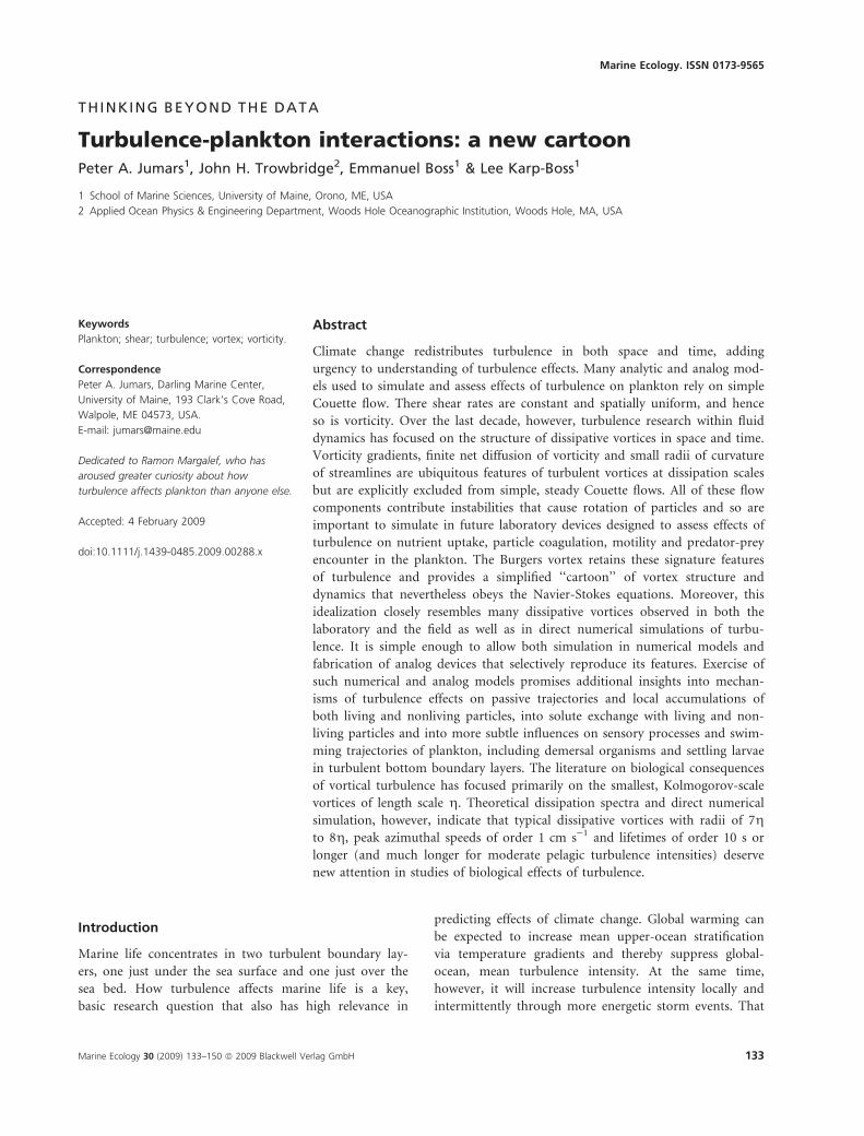
idea that a turbulent flow is a writhing tangle of vortex

‘worms’ better describes results of observations and DNS

(Fig. 1). Fluid dynamicists now dare to define turbulence

rather than continue to diagnose it from a syndrome of

characteristics: irregularity, diffusivity, large Reynolds

numbers, three-dimensional vorticity fluctuations, dissipa-

tion, and adherence to continuum mechanics (cf. Tennekes

& Lumley 1972). Davidson (2004, p. 53) has defined

hydrodynamic turbulence in an incompressible fluid as ‘a

spatially complex distribution of vorticity which advects

itself in a chaotic manner in accordance with (2.31)

[reproduced below as equation (3)]. The vorticity field is

random in both space and time, and exhibits a wide and

continuous distribution of length and time scales.’ Wu

et al. (2006, p. 106) attribute an even simpler definition of

turbulence to Bradshaw: ‘randomly stretched vortices.’



Vorticity, vortices and stretching (straining) are essential

components of the new fluid dynamics ‘cartoon.’

Reynolds numbers are dimensionless and have the gen-

eral form of a speed (u) times a length scale (l) times a

fluid density (q), all divided by a dynamic viscosity (l).

The two fluid properties are often combined into a kine-

matic viscosity, m = l ⁄ q, reducing the number of terms

to three: ul ⁄ m. Variety in Reynolds numbers (Re) is limit-

less and depends on choice of length and speed scales.

A generally useful body Re for particle motion chooses

particle radius as the length scale and relative speed of the

particle to that of the far-field surrounding fluid as the

speed scale. We later will also introduce two more

Reynolds numbers specific to vortices. Re can be inter-

preted generally as the ratio between inertial and viscous

forces within a specific flow. Higher Re implies greater

turbulence intensity.

Before we introduce additional equations, we should

comment on notation. Vorticity, x, is a vector quantity,

but only magnitude and not direction of rotation in iso-

tropic turbulence is important to our arguments, and at

dissipation scales in intense, isotropic turbulence there is

no bias of one direction of rotation over the other.

Therefore, we largely avoid the added distraction of

vector notation, with the single exception of Fig. 2, where

direction determines sign. There and elsewhere, we com-

pletely arbitrarily show velocity profiles for counterclock-

wise-rotating vortices (looking at them from the top),

which by the right-hand convention makes vorticity posi-

tive. Half the vortices in isotropic turbulence will oppose

that direction of rotation; we work far below the scale

where Coriolis effects become significant.

Evaluation of turbulence effects on organisms clearly

has not reached the new, vorticity-focused, textbook-level

understanding of turbulence. Steady, Couette flow by

design is one dimensional, with constant shear orthogonal

to the driving surface(s). Toward the goal of simplicity in

representation and analysis, vorticity is constrained to be

parallel to the driving surface(s). The vorticity equation

(where both x and u are vectors) can be written as

DxDt¼ x � rð Þuþ mr2x: ð3Þ

It is sound practice to start with a simplified mathemat-

ical basis, make sure that everything works, and interpret

those results and their limitations before moving toward

the realism and added complexity of fully 3D solutions

and time variation. For turbulence, however, the path

must be followed into 3D because in 2D the first term on

the right of equation (3) equals zero, so only viscous

forces (through diffusion of vorticity via the second term

on the right) can alter vorticity in a 2D flow. In 2D, signa-

ture features of turbulence at dissipation scales thus are

missing: Vortex stretching cannot occur, and any vorticity

is confined to the axis orthogonal to the two dimensions

of the system that are explicitly modeled. In steady

Couette flow, vorticity shows no net diffusion because it is

constant throughout; both terms on the right are exactly

zero. In and near real vortices, however, vorticity diffuses

down gradients. Couette flow can produce realistic views

neither of the deformations that vortical flows produce in

both chemical boundary layers and plumes nor of transla-

tion, rotation and deformation of cells and chains caused

by fluid motion in and near vortices.

By definition, vortices are coherent fluid motions in

the two dimensions perpendicular to their axes rather

than random or chaotic fluctuations in all three spatial

dimensions. Vortical stirring can bring reactants together

in ways that random fluctuations cannot (Crimaldi et al.

2006), with abundant ecological consequences (e.g.

Crimaldi & Browning 2004). The high shear and diffusing

vorticity between a dissipative eddy and its surrounding

medium are likely to have profound effects on small

organisms. The question that we pursue here is how to

select and utilize a physical cartoon of dissipative-scale

vortices to improve understanding of turbulence effects

on those organisms.

748η

748η

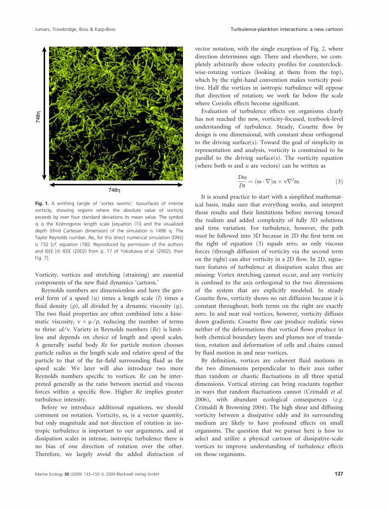
Fig. 1. A writhing tangle of ‘vortex worms’: Isosurfaces of intense

vorticity, showing regions where the absolute value of vorticity

exceeds by over four standard deviations its mean value. The symbol

g is the Kolmogorov length scale [equation (1)] and the visualized

depth (third Cartesian dimension) of the simulation is 1496 g. The

Taylor Reynolds number, Rek for this direct numerical simulation (DNS)

is 732 [cf. equation (18)]. Reproduced by permission of the authors

and IEEE [ª IEEE (2002) from p. 17 of Yokokawa et al. (2002), their

Fig. 7].



Axial symmetry is appropriate for the simplest vortex

cartoon. The natural coordinate system is z for distance

along axis, r for distance perpendicular to that axis and hfor angular (azimuthal) position about the axis. Before we

consider realistic vortex structures at dissipation scales,

we work through a succession of vortex cartoons of

increasing complexity, a line vortex, a Rankine combined

vortex, the intuitive but complex ‘bathtub vortex’ and

one simplified viscous vortex. The simplest vortices are

inviscid. In the absence of viscosity, the second term on

the right of equation (3) equals zero, so only vortex

stretching (or its opposite) can alter vorticity. Inviscid

vortices provide useful contrasts with vortices that are

substantially affected by viscosity.

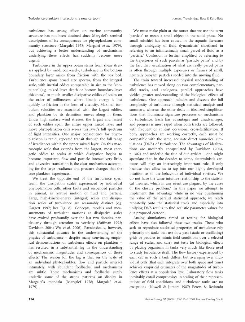
Our first vortex cartoon is the idealized line vortex

(e.g. Batchelor 1967), in which both axial and radial

velocity components are zero, axial vorticity is concen-

trated in a singularity at the origin (r = 0), and azi-

(A)

(B)

(C)

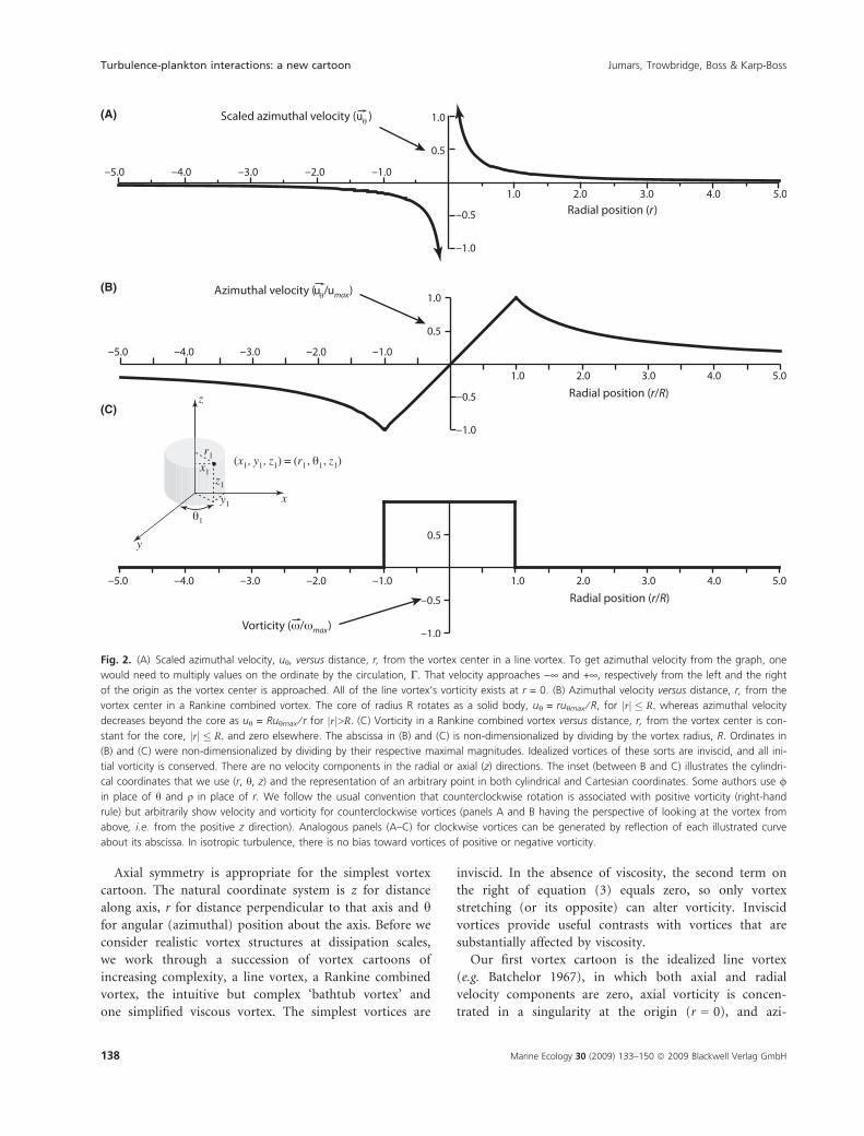
Fig. 2. (A) Scaled azimuthal velocity, uh, versus distance, r, from the vortex center in a line vortex. To get azimuthal velocity from the graph, one

would need to multiply values on the ordinate by the circulation, C. That velocity approaches )¥ and +¥, respectively from the left and the right

of the origin as the vortex center is approached. All of the line vortex’s vorticity exists at r = 0. (B) Azimuthal velocity versus distance, r, from the

vortex center in a Rankine combined vortex. The core of radius R rotates as a solid body, uh = ruhmax ⁄ R, for rj j � R; whereas azimuthal velocity

decreases beyond the core as uh = Ruhmax ⁄ r for rj j>R: (C) Vorticity in a Rankine combined vortex versus distance, r, from the vortex center is con-

stant for the core, rj j � R; and zero elsewhere. The abscissa in (B) and (C) is non-dimensionalized by dividing by the vortex radius, R. Ordinates in

(B) and (C) were non-dimensionalized by dividing by their respective maximal magnitudes. Idealized vortices of these sorts are inviscid, and all ini-

tial vorticity is conserved. There are no velocity components in the radial or axial (z) directions. The inset (between B and C) illustrates the cylindri-

cal coordinates that we use (r, h, z) and the representation of an arbitrary point in both cylindrical and Cartesian coordinates. Some authors use /

in place of h and q in place of r. We follow the usual convention that counterclockwise rotation is associated with positive vorticity (right-hand

rule) but arbitrarily show velocity and vorticity for counterclockwise vortices (panels A and B having the perspective of looking at the vortex from

above, i.e. from the positive z direction). Analogous panels (A–C) for clockwise vortices can be generated by reflection of each illustrated curve

about its abscissa. In isotropic turbulence, there is no bias toward vortices of positive or negative vorticity.



muthal velocity, uh (Fig. 2A), is given by C ⁄ (2pr), where

C [L2ÆT)1] is vortex strength or circulation, defined for-

mally as the line integral around a closed path sur-

rounding the origin in the r–h plane. [Acheson (1990)

provides a highly accessible introduction to the concept

of circulation and its application.] Viscous terms in the

equation of motion are identically zero for r > 0 in the

idealized line vortex.

Our second vortex cartoon is the Rankine combined

vortex, so named because the central core behaves very

differently from the outer flow field (Fig. 2B, C). Flow

again is exclusively azimuthal. Velocity increases linearly

from the center of the vortex to a maximum, uhmax, at

the outer edge of the core (defined as r = R). The region

r < R lacks shear. In this core, all motion is as though in

solid-body rotation, i.e. as if the water and everything

suspended in it were frozen and spinning literally like a

top. Vorticity in the core therefore is constant and falls

abruptly to zero beyond R, where azimuthal velocity falls

off as uhmax ⁄ r. Tornadoes and dust devils often approxi-

mate this structure. As they left Kansas, Dorothy and

Toto remained at a constant distance from and in fixed

orientation to each other, while each was spun around to

face each compass point exactly once in each complete

rotation of the tornado. This kind of vortex also has rele-

vance to plankton and the larger scales of turbulence,

whose statistics generated by DNS can be surprisingly well

simulated by invoking a spectrum of inertial-scale, ran-

domly oriented, Rankine vortices (He et al. 1999). The

combined Rankine vortex requires that the fluid be invis-

cid, so that the second term on the right of equation (3)

equals zero. Inviscid vortices are useful as simpler end

members to contrast with flows that are substantially

affected by viscosity.

Our third vortex cartoon, perhaps the most familiar

but also the most complex in this series of three, forms

when a large tub of water drains through a relatively

small opening in its bottom in the presence of system

rotation at angular velocity X [T)1]. (If the tub is fixed

to the rotating earth, then X is the local vertical compo-

nent of the angular velocity of the earth; if the tub is

fixed to a rotating laboratory table, then X is the angular

velocity of the table). At large scale (ffiffiffiffiffiffiffiffiffim=X

psmall com-

pared with the water depth and tub radius), inward radial

velocity toward the drain is confined primarily to a rela-

tively thin ‘Ekman’ layer of thicknessffiffiffiffiffiffiffiffiffim=X

pover the tub

bottom, and vertical velocity is confined primarily to the

narrow core of the vortex (Andersen et al. 2003). Outside

of the vortex core and away from the tub boundaries, vis-

cosity is again unimportant, and azimuthal velocity uh is

given approximately by X r + C ⁄ r, where the vortex

strength C is given in this case by FffiffiffiffiffiffiffiffiffiX=m

p �p; with F

[L3ÆT)1] being the volume flow rate exiting the tub

(Andersen et al. 2003). Vertical flow produced by gravity

is providing the vortex stretching. Where Xr is small, as

in a common bathtub, uh is approximately C ⁄ r, so its

profile with r resembles that of a line vortex (Fig. 2A). In

a bathtub vortex, the radial pressure gradient is apparent

as a depression of steeply increasing depth toward the

vortex center.

We introduce this relatively complex vortex because it

connects a commonly experienced flow with the other-

wise abstract idea of vortex stretching as a means to

accelerate azimuthal flow. It also dramatically visualizes

the otherwise nearly invisible role of pressure in vortical

flow at small scale. Lower-than-ambient pressure along

the axis is common to all small vortices but is blatantly

obvious only in the bathtub vortex. Whether its vorticity

is positive or negative – even for a weakly spinning, vis-

cous vortex – careful examination of the water surface

will reveal a dimple where a vortex axis intersects the

water surface. Low pressure provides the centripetal forces

that keep the fluid from following a straight path. The

spinning liquid itself exerts the centrifugal forces that

dynamically maintain this same negative pressure, and the

overall dynamic stability of net forces in the spinning

fluid underlies the clear prevalence of vortices in turbu-

lence (Fig. 1).

The presence of viscosity

Viscosity destroys singularities and local steepness in one-

dimensional velocity gradients. The simplest viscous vor-

tex can be described as a desingularization of a line vortex

(Lamb 1932; Batchelor 1967), and is termed the

Lamb–Oseen vortex by Saffman (1992), who gives analytic

solutions for the resultant, circular velocity and vorticity

fields. These solutions are consistent with the Navier–

Stokes equations. Viscous diffusion acts quickly on small

scales to move uh as a function of r toward Gaussian

shape. For an initial circulation, C0, concentrated at the

origin (Saffman 1992, p. 253):

uh ¼C

2pr¼ C0

2pr1� e�r2=4mt� �

; ð4Þ

xz ¼C0

4prmte�r2=4mt ; ð5Þ

C ¼ C0 1� e�r2=4mt� �

: ð6Þ

Here t is time. To be perfectly clear, Lamb–Oseen and

line vortices are identical and do have a singularity at

r = 0, t = 0, before viscosity has had time to act, but vis-



cosity will erase the singularity in less than a millisecond.

Small, axisymmetric vortices that lack any driving forces

to keep them spinning differently will spin down toward

this shape under the influence of viscosity no matter

whether they begin as line vortices, Rankine vortices or

something more complex. Their characteristic Gaussian

shape in radial velocity and vorticity profiles results from

the way that momentum and vorticity diffuse away from

axial regions of high values in a cylindrical geometry.

Two vortical structures have emerged repeatedly from

both very accurate DNS of turbulence and model simplifi-

cations. Both are consistent with the Navier–Stokes equa-

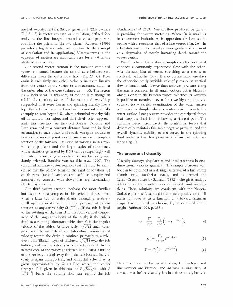
tions. The first is the Burgers (1948) vortex (Fig. 3) that

accommodates extensional straining along its axis of vor-

ticity and for realistic conditions satisfies the Navier–

Stokes equations. The opposite pattern of straining (one

compressional strain rate and orthogonal extensional

straining along the other two axes) appears to be even

more common (Davidson 2004) and produces vortex

sheets. They are unstable, however (as evidenced by the

dominance of vortices over sheets in Fig. 1), and tend to

roll up and evolve into something approximating the sec-

ond kind of vortex, the Lundgren (1982) stretched-spiral

vortex, for which asymptotic solutions are available (Pullin

& Saffman 1998). For diagrams of the bursting and folding

steps, see Davidson (2004, p. 207). Furthermore, the Lund-

gren stretched-spiral vortex decays asymptotically toward

the structure of the Burgers vortex (Pullin & Saffman

1998), justifying our focus here on the latter as a simplify-

ing cartoon. Prevailing structures in turbulence clearly are

elongate vortices (axial length >> radius, Fig. 1).

Views regarding the applicability of the Burgers (1948)

vortex have changed remarkably through DNS. Not long

ago (e.g. Acheson 1990) this Navier–Stokes solution was

considered a curiosity because no obvious spatial and

velocity scales emerged with it. Hatakeyama & Kambe

(1997), however, found that an ensemble of Burgers vor-

tices with random orientations and strengths provides an

accurate description of longitudinal structure functions

observed in laboratory measurements and DNS of homo-

geneous, isotropic turbulence at dissipative scales, pro-

vided that a realistic probability density function for

vortex strengths is incorporated in the calculation. In

spite of limitations pointed out by He et al. (1999), the

random Burgers vortex model thus is a potentially useful

idealization for studying interactions between turbulence

and plankton at dissipative scales.

In a steady Burgers vortex, viscous dissipation continu-

ously removes kinetic energy from the flow, but velocities

remain constant because a constant, local, axial strain at

rate, cloc [T)1], continuously accelerates the fluid azi-

muthally. [Note that Davidson (2004]) and some other

authors use a ⁄ 2 in place of cloc; we reserve a for the

dimensionless Kolmogorov constant.] Through continu-

ity, inward radial flow supports this axial straining.

Inward advection of vorticity and of azimuthal momen-

tum by this flow balances their outward diffusion. In a

steady Burgers vortex,

rB ¼ffiffiffiffiffiffiffi2mcloc

s; ð7Þ

cloc ¼2mr2

B

ð8Þ

(Davidson 2004). Axial vorticity, tangential velocity and

local dissipation rates show characteristic shapes as func-

tions of non-dimensional radius, br ¼ r=rB (He et al. 1999;

Fig. 4 herein):

uh ¼C

2prB

1� e�br 2

br !

; ð9Þ

xz ¼C

pr2B

e�br 2

; ð10Þ

ur ¼ �clocr; ð11Þ

uz ¼ clocz: ð12Þ

Fig. 3. Cartoon of a steady Burgers (1948) vortex. Constant tensile

straining at rate cloc would accelerate the rotation (conserving vortici-

ty) by thinning the vortex (reducing its radius) if outward diffusion of

vorticity did not counterbalance this effect. Vorticity remains steady

because its constant diffusion outward is counterbalanced exactly by

the combination of inward advection and vortex stretching. Modified

from Acheson (1990, p. 188) and Davidson (2004, p. 249).



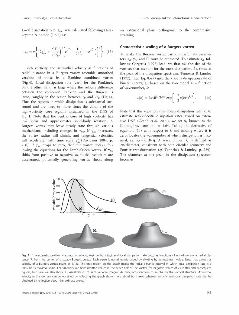
Local dissipation rate, eloc , was calculated following Hata-

keyama & Kambe (1997) as:

eloc ¼ m 12c2loc þ

Cpr2

B

� �2

e�br 2 � 1br 21� e�br 2� �� 2

( ): ð13Þ

Both vorticity and azimuthal velocity as functions of

radial distance in a Burgers vortex resemble smoothed

versions of those in a Rankine combined vortex

(Fig 4). Local dissipation rate (zero for the Rankine),

on the other hand, is large where the velocity difference

between the combined Rankine and the Burgers is

large, roughly in the region between rB and 2rB (Fig 4).

Thus the regions in which dissipation is substantial sur-

round and are three or more times the volume of the

high-vorticity core regions visualized in the DNS of

Fig. 1. Note that the central core of high vorticity has

low shear and approximates solid-body rotation. A

Burgers vortex may leave steady state through various

mechanisms, including changes in cloc. If cloc increases,

the vortex radius will shrink, and tangential velocities

will accelerate, with time scale c�1loc (Davidson 2004, p.

250). If cloc drops to zero, then the vortex decays, fol-

lowing the equations for the Lamb–Oseen vortex. If cloc

shifts from positive to negative, azimuthal velocities are

decelerated, potentially generating vortex sheets along

an extensional plane orthogonal to the compressive

straining.

Characteristic scaling of a Burgers vortex

To make the Burgers vortex cartoon useful, its parame-

ters, rB, cloc and C, must be estimated. To estimate rB, fol-

lowing Gargett’s (1997) lead, we first ask the size of the

vortices that account for the most dissipation, i.e. those at

the peak of the dissipation spectrum. Tennekes & Lumley

(1972), their Eq. 8.4.7) give the viscous dissipation rate of

kinetic energy, em, based on the Pao model as a function

of wavenumber, k:

em kð Þ ¼ 2ame2=3k1=3 exp � 3

2a kgð Þ4=3

� : ð14Þ

Note that this equation uses mean dissipation rate, e, to

estimate scale-specific dissipation rates. Based on exten-

sive DNS (Gotoh et al. 2002), we set a, known as the

Kolmogorov constant, at 1.64. Taking the derivative of

equation (14) with respect to k and finding where it is

zero, locates the wavenumber at which dissipation is max-

imal, i.e. kd = 0.18 ⁄ g. A wavenumber, k, is defined as

2p ⁄ diameter, consistent with both circular geometry and

Fourier transformation (cf. Tennekes & Lumley, p. 259).

The diameter at the peak in the dissipation spectrum

becomes

Fig. 4. Characteristic profiles of azimuthal velocity (uh), vorticity (xz), and local dissipation rate (xloc) as functions of non-dimensional radial dis-

tance, br, from the center of a steady Burgers vortex. Each curve is non-dimensionalized by dividing by its maximum value. Note that azimuthal

velocity of a Burgers vortex peaks at 1.12br. The gray region on the graph marks the radial distance interval in which local dissipation rate is ‡50% of its maximal value. For simplicity we have omitted values in the other half of the vortex (for negative values of br ) in this and subsequent

figures, but here we also show 3D visualizations of each variable (magnitude only, not direction) to emphasize the vortical structure. Azimuthal

velocity in this domain can be obtained by reflecting the graph shown here about both axes, whereas vorticity and local dissipation rate can be

obtained by reflection about the ordinate alone.



d ¼ 11pg: ð15Þ

The corresponding radius, a more useful measure of

distance for our subsequent purposes, is 17.5g. By

integrating equation (14) with respect to k, we also cal-

culate that 90% of dissipation occurs in the eddy

radius range of 2.7g to 58g. One-half of the dissipa-

tion is associated with vortices >8.1g in radius. Because

equation (14) and most other distributions that we will

treat are asymmetric, we choose to use median rather

than mean values as being ‘typical’; although 8.1g is

not a median radius, it applies a similarly tail-insensi-

tive method to deal with the asymmetry of equation

(14). Once rB is determined (d ⁄ 2), equation (8) reveals

the local strain rate, cloc , required to maintain a Burg-

ers vortex of that radius in steady state. The path to Cestimates is a bit more circuitous.

Taylor (1921) introduced k, later named the Taylor

microscale, as an intermediate spatial scale at which dissi-

pation rate, kinetic energy of the flow, and viscosity all

interact:

e ¼ 15mu2

rms

k2 ; ð16Þ

k ¼ffiffiffiffiffiffiffiffi15me

rurms ð17Þ

(e.g. Frisch 1995; Eq. 2.28 and 5.10). It falls between

dissipation and integral length scales. To connect Taylor’s

derivation with equations (16) and (17), we make use of

the equality of e and mxixi, where xi is the ith compo-

nent of vorticity (e.g. Frisch 1995, p. 21), in Frisch’s

expression for k. The length and velocity scales, in turn,

can be used to form a Taylor Reynolds number,

Rek ¼urmsk

m; ð18Þ

that further characterizes flow at this intermediate scale

where inertial energy is spilling into the dissipation spec-

trum. Kolmogorov (1941) hypothesized that small-scale

turbulence statistics depend on e and m alone, but –

because of intermittency – these two parameters have

proven insufficient to determine urms (Frisch 1995). That

is, the same e can result from flows that vary in intermit-

tency and hence in urms. We therefore need a way to

choose an appropriate urms.

Direct numerical simulations have revealed statistical

regularities that aid in estimating the remaining Burgers

vortex parameter and use the quantities in equations

(16)–(18). Hatakeyama & Kambe (1997) sought to

analyze the distribution of vortex Reynolds numbers, ReC,

defined as

ReC ¼Cm: ð19Þ

They assumed for isotropic turbulence that mean strain

rate

c ¼ urms

2k; and ð20Þ

C ¼ 2prBurms ð21Þ

Consequently, the mean value for the fraction is

ReCffiffiffiffiffiffiffiRekp ¼ 4p: ð22Þ

Hatakeyama & Kambe (1997) found that equation (22)

fits the central tendency for previously published DNS

very well, supporting our use of equation (21) to estimate

C. They used DNS results further to characterize the dis-

tribution of ReC about this mean tendency and proposed

that the ReC has a probability density function,

PReC ReCð Þ,given by

PReC ReCð Þ ¼ C 3

2Re2

C exp �CReCð Þ; ð23Þ

where, in order to conform to equation (22),

C ¼ 3

4pffiffiffiffiffiffiffiRekp : ð24Þ

The expression for C in note [21] of Hatakeyama &

Kambe (1997) contains a typographical error that has

been corrected here. The expected or mean value of ReC

based on the model distribution is 4pRek1 ⁄ 2, as per equa-

tion (22). Ninety percent of ReC values would fall

between 0.27 and 2.1 times that mean value, however,

and the same proportional range from its mean would be

expected for C [equation (19)]. The most frequent

(modal) ReC and C are two-thirds of their respective

mean values, whereas the medians are 0.89 times the

means.

He et al. (1999) adopted the Hatakeyama & Kambe

(1997) distribution of ReC and further proposed, based on

previously published DNS, that the dimensionless Burgers

radius, er ¼ rB=g, has a probability density, PCB, given by

PCBerBð Þ ¼ Eer 2

B exp �er 0:7B

�: ð25Þ

E in turn is a normalization constant given by



E�1 ¼Z þ1

0

er 2B exp �er 0:7

B ÞderB:

ð26Þ

The expected value (mean) of rB based on this

approach is approximately, 8.5g and the median is 7.1g,

both remarkably close to the median-like value of 8.1gobtained from the dissipation spectrum. Good correspon-

dence of these two approaches in identifying a ‘typical’

Burgers vortex radius gives some confidence that the

choice is a good one, and each approach also permits

examination of the broader spectrum of dissipation-scale

vortices. Ninety percent of Burgers vortex radii under

equation (25) fall between 1.8g and 20g.

We first estimate the parameters of the Burgers vortex

in the simplest and longest-studied kind of boundary

layer, i.e. the boundary layer produced by steady, horizon-

tally uniform, unidirectional (in the mean) flow over wall

or sea floor of uniform roughness, a so-called ‘wall layer.’

In a crude way, a bottom boundary layer is kinematically

similar to an upside-down upper mixed layer. It is simpler

in some ways because the geometry of the sediment-water

interface evolves more slowly than the air–sea interface.

The presence of the more-or-less rigid wall, however, cre-

ates some important differences. Following the normal

convention, we use positive x for the downstream direc-

tion, y for the cross-stream dimension and z for the verti-

cal dimension, and u, v and w for the respective velocity

components. Here we will use u, v and w explicitly to refer

to the fluctuating components of velocity (elsewhere often

denoted with an apostrophe). We follow the usual con-

vention of z being positive upward from the sea bed. Vor-

ticity is generated at the sea bed in the y direction and has

the same direction of rotation as would a bicycle tire roll-

ing downstream over the sea bed. In proximity to the wall,

turbulent vortices retain some of this bias toward rotating

about a cross-stream axis, and vertical velocities are sup-

pressed by the low-permeability wall.

As a specific example, we consider the wall layer of an

unstratified bottom boundary layer. The ensemble-aver-

aged dissipation is approximately (e.g. Thorpe 2007, p. 86)

e ¼ u3�

jz; ð27Þ

where u� is the shear velocity and j . 0.41 is von

Karman’s constant. Shear velocity is estimated from verti-

cal profiles of horizontal velocity (e.g. Gross & Nowell

1983). Following Monin & Yaglom (1971, p. 280), stan-

dard deviations of the velocity components are

u2 �1=2

; v2 �1=2

; w2 �1=2

h i’ 2:3; 1:7; 0:9½ �u�; ð28Þ

so that

urms ’1

32:32 þ 1:72 þ 0:92 �� 1=2

u� ’ 1:7u�: ð29Þ

For m = 10)6 m2Æs)1, u� = 10)2 mÆs)1 (a value near the

critical erosion threshold for many unconsolidated sedi-

ments) and z = 2.5 m, equation (27) yields

e ¼9.8 · 10)7 m2Æs)3. Further, g = 1.0 · 10)3 m [equa-

tion (1)], rB . 7.1 mm [7.1g, median of equation (25)],

urms . 1.7 · 10)2 mÆs)1 [equation (29)], k . 6.7 ·10)2 m [equation (17)] and Rek . 1.1 · 103 [equation

(18)]. The remaining Burgers parameters become

cloc = 3.9 · 10)2 s)1 [equation (8)] and C = 7.6 ·10)4 m2Æs)1 [equation (21)]. Using median values of the

proposed distribution [equation (23)], one finds

ReC . 3.8 · 102. With these values, the Burgers vortex

solution [equation (9)–(13)] gives max (uh) . 1.1 cmÆs)1,

max (eloc) . 2.1e and max (xz) . 4.8 s)1.

Estimation of the Burgers vortex parameters in an

upper mixed layer can be complicated by the interaction

of gravity waves with turbulent motions. Such interac-

tions have been the subject of extensive research. Here we

use simplified results based on recent field measurements

and scaling arguments to provide quantitative estimates

of the relevant scales; the results do not account explicitly

for quasi-coherent processes such as Langmuir circula-

tions (e.g. Thorpe 2007), although these processes are

likely incorporated in the empirical results.

Significant wave height, Hs [m] is the vertical peak-to-

trough distance. When waves break, motions within this

region (with the interface z = 0 defined as the midpoint

between peak and trough and increasing depth being con-

sidered positive z) are very time- and location-dependent.

The region from the wave trough to a depth of order

10Hs is called the wave-affected surface layer. Unlike the

classic wall model, where turbulent kinetic energy comes

entirely from vertical shear, in this region turbulent

kinetic energy derives primarily from downward transport

of kinetic energy injected by waves breaking above (Gerbi

et al. 2009, their Fig. 1). In the wave-affected surface

layer, mean dissipation rate can be written

e ¼ 0:3Gtu

3�Hs

z2; ð30Þ

where Hs is the significant wave height and Gt is a dimen-

sionless parameter that expresses the ratio between u3� and

the energy flux from the wind to the waves, which ranges

between approximately 90 and 250 for all but extremely

young seas (Terray et al. 1996). Gerbi et al. (2009) found

that a value of 168 provided the best fit of their observa-

tions to the scaling of Terray et al. (1996). Terray et al.

(1996), Drennan et al. (1996), Feddersen et al. (2007),

Jones & Monismith (2008), and Gerbi et al. (2009)



showed that equation (30) describes near-surface dissipa-

tion in a variety of field measurements. Burchard (2001)

showed that an appropriately modified, two-equation tur-

bulence model [equation (30) for the wave-affected layer

and equation (27) for the layer below it] reproduces the

observed dissipation structure. Gerbi et al. (2009) found

field measurements of velocity variance in the wave-

affected surface layer to be consistent with

q3 ¼ Kez; ð31Þ

where q2 ¼ 1=2ð Þ u2 þ m2 þ w2 �

is the turbulent kinetic

energy per unit of mass and K is an empirical constant

with a median value of approximately 1.34. Measure-

ments of w2 reported by Gerbi et al. (2009) are consistent

with those of D’Asaro (2001) and Tseng & D’Asaro

(2004). It follows from the above expression and the defi-

nitions of q2 and urms that in the wave-affected surface

layer

urms ¼2

3

� �1=2

Kezð Þ1=3: ð32Þ

Terray et al. (1996) estimated that the wave-affected

surface layer is bounded by

0:6 � z

Hs� 0:3jGt : ð33Þ

The upper bound is obtained by equating the expressions

for dissipation in the wave-affected surface layer and wall

layer. Depth of the transition varies with time since onset

of wind and peaks at intermediate wave age, when it can

be as large as 25Hs (Terray et al. 1996, their Fig. 8).

We use the Gerbi et al. (2009) results to produce a

sample calculation. We emphasize that these results are

by no means extreme and are limited to significant wave

heights of about 1 m or less at the Martha’s Vineyard

Cabled Observatory (MVCO) off the coast of Massachu-

setts, USA, during October 2003, in waters about 15 m

deep. Data are available online at http://www.whoi.edu/

mvco/data/oceandata.html. From the temperature and

salinity, we estimate a kinematic viscosity of about

1.14 · 10)6 m2Æs)1. Gerbi et al. (2009, their Fig. 6)

observed several episodes when e in the wave-affected

layer reached 10)5 m2Æs)3. From equation (32), we obtain

an estimate of urms = 2.6 cmÆs)1. Values of urms this large

are supported by both the measurements of Gerbi et al.

(2009) and estimates from float data by Tseng & D’Asaro

(2004) for the open-ocean North Pacific in the same sea-

son (October–November, when kinematic viscosities,

dominated by temperature, were also similar). During this

season, mixed-layer depth is gradually increasing, and

stratification plays no large role in dynamics near the air–

water interface. We estimate median rB [7.1g from equa-

tion (1)] to be 4.4 mm and k [equation (17)] to be

3.4 cm. Strain rate [equation (8)] for a steady Burgers

vortex of this radius is 0.12 s)1 and circulation,

C = 7.2 · 10)4 m2Æs)1 [equation (21)]. With these values,

the Burgers vortex solution [equation (9)–(13)] gives

max (uh) . 1.7 cmÆs)1, max (eloc) . 1.4 e and max

(xz) . 12 s)1.

How long does this typical Burgers vortex last? To gain

some idea, we calculate its decay by noting that a vortex

with identical azimuthal velocity and axial vorticity can

be produced by viscous decay from a line vortex that has

initial circulation, C0, equal to the steady value of C for

the Burgers vortex in question (Davidson 2004, Problem

5.3, p. 291). This equivalence is most easily demonstrated

by noting that the Burgers equations for azimuthal veloc-

ity and axial vorticity can be recovered by substituting

the quantity r2B

�4m ¼ c�1

loc

�2 for t in equations (4) and (5)

(representing an e-folding time, i.e. the time to decay to

1 ⁄ e or about 0.37 times the initial value). This necessary

correspondence allows calculation of decay dynamics

under the scenario of a steady Burgers vortex for which

strain rate, cloc, goes instantaneously to zero (Fig. 5A–C).

We set initial (time-zero) circulation at

C0 = 7.6 · 10)4 m2Æs)1 and find [equation (4)] that it

takes 4.3 s to decay to the azimuthal velocity profile of

our typical Burgers vortex. We observe that a natural

time scale for decay of a Burgers vortex, sd, once straining

has stopped is the inverse of the strain rate that is needed

to keep it in steady state, i.e. sd = 1 ⁄ cloc = 8.5 s for the

upper mixed-layer example. Because we have deliberately

chosen very energetic upper mixed-layer turbulence, this

time is unusually short. For the bottom boundary-layer

example sd is substantially longer (26 s) because median

rB is somewhat larger.

All these values are remarkably larger than intuition

might suggest from working at the Kolmogorov scale

[equation (1)]. For explicit comparison, the Kolmogorov

time scale, sg, and velocity scale, ug, for this upper

mixed-layer example are:

sg ¼me

� �1=2

¼ 0:34 s; ð34Þ

ug ¼ með Þ1=4¼ 1:8 mm � s�1: ð35Þ

Better intuition comes from inspection of equation (8).

The time scale for decay is proportional to the square of

the vortex radius and inversely proportional to twice the

kinematic viscosity. This observation helps to explain why

eddies of the size at the mode of equation (14) are sub-



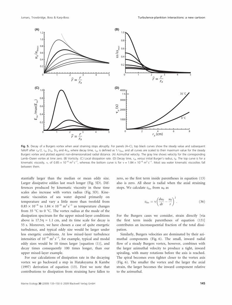
stantially larger than the median or mean eddy size.

Larger dissipative eddies last much longer (Fig. 5D). Dif-

ferences produced by kinematic viscosity in these time

scales also increase with vortex radius (Fig. 5D). Kine-

matic viscosities of sea water depend primarily on

temperature and vary a little more than twofold from

0.85 · 10)6 to 1.84 · 10)6 m2Æs)1 as temperature changes

from 35 �C to 0 �C. The vortex radius at the mode of the

dissipation spectrum for the upper mixed-layer conditions

above is 17.5g = 1.1 cm, and its time scale for decay is

55 s. Moreover, we have chosen a case of quite energetic

turbulence, and typical eddy size would be larger under

less energetic conditions. At low mixed-layer turbulence

intensities of 10)9 m2Æs)3, for example, typical and modal

eddy sizes would be 10 times larger [equation (1)], and

decay times consequently 100 times longer, than our

upper mixed-layer example.

For our calculations of dissipation rate in the decaying

vortex we go backward a step in Hatakeyama & Kambe

(1997) derivation of equation (13). First we note that

contributions to dissipation from straining have fallen to

zero, so the first term inside parentheses in equation (13)

also is zero. All shear is radial when the axial straining

stops. We calculate eloc from uh as

eloc ¼ mduh

dr� uh

r

� �2

: ð36Þ

For the Burgers cases we consider, strain directly [via

the first term inside parentheses of equation (13)]

contributes an inconsequential fraction of the total dissi-

pation.

Similarly, Burgers velocities are dominated by their azi-

muthal components (Fig. 6). The small, inward radial

flow of a steady Burgers vortex, however, combines with

the larger azimuthal velocity to produce a tight, inward

spiraling, with many rotations before the axis is reached.

The spiral becomes even tighter closer to the vortex axis

(Fig. 6). The smaller the vortex and the larger the axial

strain, the larger becomes the inward component relative

to the azimuthal.

(A) (B)

(C) (D)

Fig. 5. Decay of a Burgers vortex when axial straining stops abruptly. For panels (A–C), top black curves show the steady value and subsequent

falloff after sd ⁄ 2, sd, 2sd, 3sd and 4sd, where decay time, sd, is defined as 1 ⁄ cloc, and all curves are scaled to their maximum value for the steady

Burgers vortex and plotted against non-dimensionalized radial distance. (A) Azimuthal velocity. The gray line shows velocity for the corresponding

Lamb–Oseen vortex at time zero. (B) Vorticity. (C) Local dissipation rate. (D) Decay time, sd, versus initial Burger’s radius, rB. The top curve is for a

kinematic viscosity, m, of 0.85 · 10)6 m2Æs)1, whereas the bottom curve is for m = 1.84 · 10)6 m2Æs)1. Most sea water kinematic viscosities fall

between them.



Some caveats are in order. Myopic focus on a single

eddy diameter and velocity scale is unwise, which is why

we present the spectral formula for dissipation and prob-

ability density functions for vortex radius and circulation.

Vortices also clearly interact with each other in important

ways, as even casual examination of Fig. 1 attests. Adja-

cent, counter-rotating vortices will translate together, and

may join to form a single, toroidal vortex, analogous to a

smoke ring in air (e.g. Thorpe 2007; his Fig. 1.9). The

pair will have lower shear between them than would exist

at the same radius from a single vortex of comparable

size and velocity, and they will pull water between them

as they migrate. Co-rotating vortices move in orbits

around each other and may coalesce to form a larger vor-

tex, but – until they do – they will have greater shear

between them than would exist at comparable radial dis-

tance from a single vortex of similar size and rotation

rate. Deformations of groups of smaller vortices by larger

ones that entwine them are evident in Fig. 1; multiple-

vortex interactions are present in much variety and will

cause local and ephemeral extremes in strain rates, shear

and dissipation. Somewhat paradoxically, these complica-

tions remove some of the early objections to Burgers vor-

tices as representations of realistic physical entities. In the

context of DNS, continued growth of velocity in the

radial and axial directions implied by equations (11) and

(12) is cut off by the action of instabilities in the form of

higher velocities imposed by neighboring vortices (Fig. 1).

All of these interactions will affect vortex lifetimes and

create extensive variation in local vorticities and dissipa-

tion rates. The cartoon of a single vortex of a given size

and velocity is simply a logical place to start to examine

vortex interactions with plankton. It should continue to

be complemented by studies of building complexity and

by studies along the statistical track.

Planktonic interactions with the cartoon vortex

Because we began with the simpler structure of a bottom

boundary layer, we also begin with a brief interpretation

of turbulence effects there. Settling larvae of limited

swimming capabilities are known to exploit suppressed

vertical velocities by swimming downward upon detection

of settling cues (e.g. Hadfield & Koehl 2004). Here we

suggest that they also exploit near-sea bed vortices of

characteristic scale and orientation. Grunbaum &

Strathmann (2003) have shown that changing offsets of

centers of buoyancy and centers of gravity during devel-

opment can bias larvae into either updrafts (favorable for

dispersal in early larval states) or downdrafts (favorable

for settlement). Regions of vortices in particular orienta-

tions both in the pelagic realm and near the bottom are

those updrafts and downdrafts, respectively. Another pos-

sibility in interpreting benthic organism form and func-

tion is that scales of benthic suspension feeders or their

feeding appendages may be matched to characteristic vor-

tex radii and tuned to vortex velocities.

In terms of phytoplankton in steady, uniaxial shear,

elongate and discoidal cells spend most of their time

aligned parallel to the velocity vectors. They tumble with

predictable frequency (Jeffery 1922), and these tumbles are

key in shedding diffusive boundary layers and contributing

to nutrient uptake (Pahlow et al. 1997). Based on our prior

experience with Jeffery orbits in Couette flow and in partic-

ular with our experience in unsteady Couette flows where

there are diffusion gradients of shear and vorticity (Fig. 7),

and thus where both velocity and vorticity change with

time at any particular location, we predict that non-spheri-

cal particles in the region between one and two Burgers

radii from the axis will tumble much more often than in a

steady, linear shear. Inward radial flow into steady Burgers

vortices and into Burgers vortices whose axial strain rates

are accelerating is also of relevance in moving the cells

themselves into different portions of the vortex. Clearly the

Burgers vortex is a more accurate cartoon of natural turbu-

lence than is Couette flow.

In atmospheric sciences, it is generally accepted that

isotropic turbulence can act size selectively to increase

droplet–droplet collision rates, to increase droplet fall

velocities and to produce particle distributions that are

nonrandom in space (e.g. Ghosh et al. 2005). A relevant

criterion is the Stokes number, Stk, the non-dimensional

ratio of the time that it takes a particle to respond to a

change in fluid flow velocity relative to the time scale

over which fluid velocity itself changes, so Stk << 1 indi-

cates that particles will follow streamlines closely; at small

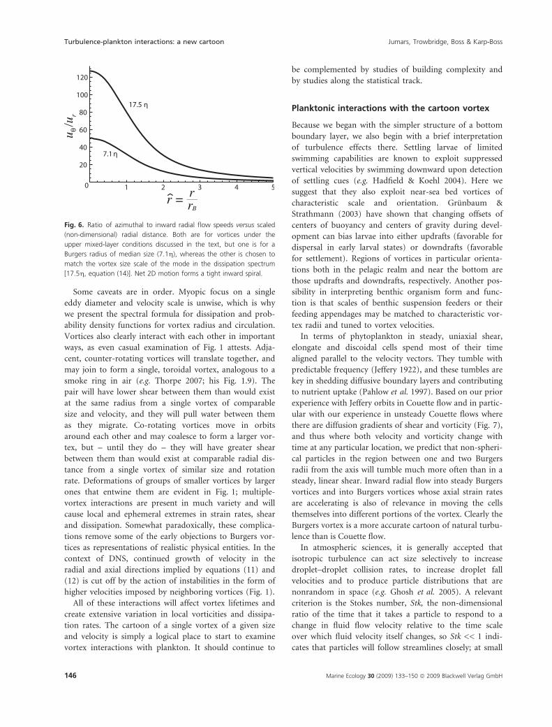
Fig. 6. Ratio of azimuthal to inward radial flow speeds versus scaled

(non-dimensional) radial distance. Both are for vortices under the

upper mixed-layer conditions discussed in the text, but one is for a

Burgers radius of median size (7.1g), whereas the other is chosen to

match the vortex size scale of the mode in the dissipation spectrum

[17.5g, equation (14)]. Net 2D motion forms a tight inward spiral.



Stk, fluid motion controls particle motion. Particle–flow

interaction will be strongest for Stk near unity. Stk >> 1,

on the other hand, indicates that the particle will move

through a vortex before it can respond to the local fluid

motion; at large Stk, particle motion dominates over fluid

motion. Centrifuging of negatively buoyant water droplets

for Stk near unity increases their fall velocities and con-

tributes to droplet growth (collision of smaller droplets)

through two mechanisms. It lowers particle abundance in

vortices and raises particle concentrations outside them.

Because collision rates go up non-linearly with droplet

concentration (i.e. with concentration squared), locally

increased concentrations raise encounter and coagulation

rates. Response of particles to turbulent fluctuations also

generally increases particle relative velocities and thus

encounter rates over those that would occur in still air

from differential deposition alone (Vaillancourt & Yau

2000; Bosse et al. 2006; Ghosh et al. 2005).

In aquatic particle dynamics, where the ratio of particle

to fluid densities is generally smaller, the contribution of

isotropic turbulence to non-random particle redistribu-

tion has been more controversial since the spotlight put

on this issue by Squires & Yamazaki (1995). In a steady

Burgers vortex, azimuthal velocity is so much larger than

the inward radial flow (Fig. 6) that particles with Stk

above a critical value will tend to find a stable radius at

which to orbit the axis, although vortex orientation with

respect to the gravitational vector matters when the parti-

cles are not neutrally buoyant (Marcu et al. 1995). At

even higher Stk, particles have sufficient inertia to be

expelled from the vortex (Ijzermans & Hagmeijer 2006).

Particles with small Stokes numbers, on the other hand,

are concentrated in the strain-dominated regions of the

flow (Bec et al. 2006;. Even neutrally buoyant spheres of

non-zero Stokes number apparently can move differen-

tially from the surrounding flow (Tallapragada & Ross

2008), although this topic remains controversial.

Much of the controversy stems from the oversimplifica-

tion of particles in the modeling done for some of these

studies that makes them ‘point particles’ that have finite

mass but infinitesimal size and no explicit shape. This

simplification cannot capture interactions of particle with

ambient flow accurately, particularly when particle sizes

approach or even exceed g (cf. Hill et al. 1992). Rarely

are all the unsteady terms, especially the wake history

terms, included in calculating particle trajectories. For

large phytoplankton cells and chains, wake history terms

can be particularly important, and their inclusion would

increase Stk for the cells (Koehl et al. 2003). The ultimate

reason for these simplifications is computational; DNS is

difficult, and realistic incorporation of particle material

properties and geometries and interactions with the flow

in DNS is still forbidding in terms of the numbers of

computations needed for realistic simulation.

Gopalan et al. (2008) put phytoplankton into isotropic

turbulence. They presented a video during the 2008

Ocean Sciences Meeting in Orlando, FL, USA, of a vortex

being stretched ()c increasing in absolute value), with

phytoplankton being concentrated along its axis in the

process. The underlying mechanism has not been clearly

(A) (B)

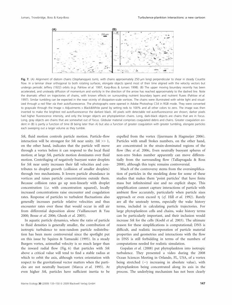
Fig. 7. (A) Alignment of diatom chains (Stephanopyxis turris, with chains approximately 250 lm long) perpendicular to shear in steady Couette

flow. In a laminar shear orthogonal to both rotating surfaces, elongate objects spend most of their time aligned with the velocity vectors but

undergo periodic Jeffery (1922) orbits (e.g. Pahlow et al. 1997; Karp-Boss & Jumars 1998). (B) The upper moving boundary recently has been

accelerated, and unsteady diffusion of momentum and vorticity in the direction of the arrow has reached approximately to the dashed line. Note

the dramatic effect on trajectories of chains, with known effects on surrounding nutrient boundary layers and nutrient fluxes (Pahlow et al.

1997). Similar tumbling can be expected in the near vicinity of dissipation-scale vortices. The chains were illuminated with white light and visual-

ized through a red filter via their autofluorescence. The photographs were opened in Adobe Photoshop CS4 in RGB mode. They were converted

to grayscale through the Image > Adjustments > Black&White panel by setting reds to 100% and all other colors to zero. The image was then

inverted to make the brightest red autofluorescence the darkest black. All pixels with detectable red autofluorescence are shown; darker pixels

had higher fluorescence intensity, and only the longer objects are phytoplankton chains. Long, dark-black objects are chains that are in focus.

Long, gray objects are chains that are somewhat out of focus. Globular material comprises coagulated debris and chains. Greater coagulation evi-

dent in (B) is partly a function of time (B being later than A) but also a function of greater coagulation with greater tumbling, elongate particles

each sweeping out a larger volume as they tumble.



identified. For positively buoyant cells, centripetal acceler-

ation might account for this concentration, or it might be

due to the strain mechanism identified by Bec et al.

(2006), or both. Shape effects also undoubtedly affect

phytoplankton trajectories in and near vortices.

Velocities of a centimeter per second and dimensions

of one to a few centimeters are also relevant to the swim-

ming and settling dynamics of small plankton, at least up

to the scales of fishes preying on copepods. That is, the

vortex radii we calculate are comparable to detection dis-

tances of copepods by fishes (e.g. Viitasalo et al. 1998),

and azimuthal velocities are comparable to or larger than

copepod cruising and sinking speeds but not as large as

copepod escape velocities (Buskey et al. 2002; Kiørboe

2008). Interaction with vortices is sure to affect the tran-

sition from ballistic to diffusive trajectories of plankton

(Kiørboe & Visser 2005); swimming tracks cannot be

independent of streamlines. Vortices quite obviously pre-

vent organisms from swimming straight through their

diameters or other secants unless swimming speeds

greatly exceed flow speeds encountered in the vortex.

Turbulence affects encounter of both inanimate particles

and organisms (e.g. Hill et al. 1992; Visser & MacKenzie

1998), so it should not be surprising that dissipative vor-

tices also have an effect.

Feasibility of numerical and analog testing

Although more complex than simple, linear shear, a

Burgers vortex is well within current numerical modeling

capabilities, so a logical way to proceed in testing effects

on passive particles such as diatoms is to embed realisti-

cally shaped and mechanically behaved model diatoms

and diatom chains in numerical models of a Burgers vor-

tex. Specifically, such objects can be embedded through

immersed boundary methods (Peskin 2002) and seeded

in various positions and orientations in and near the vor-

tex. Such numerical experiments can be used to isolate

particular regions of the vortex and parameter combina-

tions that lead to interesting tumbling behaviors, for

example, or to local concentrations of phytoplankton.

With numerical predictions in hand, it becomes much

more feasible to conduct experiments in analog devices.

Small devices already have been built to allow production

of a vortex between two parallel and synchronously rotat-

ing, circular plates. By drawing fluid through holes in the

two respective centers of those plates, vortex stretching

can be achieved (Petitjeans 2003). With commercially

available software (e.g. comsol, Burlington, MA, USA), it

is also now feasible to design small chambers a few centi-

meters long in which particular combinations of shear,

vorticity and streamline curvature duplicate selected com-

ponents of vortical flow. Indeed, such experiments have

already been done at slightly smaller scale and lower Re

(Marcos & Stocker 2006).

Conclusions

Our simple calculations in the context of the new cartoon

have changed the way that we think about turbulence by

expanding possibilities for what we conceive as mechanistic

turbulence effects over what we could imagine with the

Lazier & Mann (1989) simplification. In a bottom bound-

ary-layer setting, fish that exceed vortex diameters in length

can exploit vortices that they do not themselves generate to

gain energetic advantage in swimming (Liao et al. 2003).

Detecting a vortex, its axial orientation and its direction of

rotation are more difficult tasks for organisms smaller than

the vortex, but if resources, predators and prey are non-

randomly distributed with respect to vortex coordinates,

selection is likely to have found cues that lead individuals

toward enhanced resources and away from enhanced risks.

It would indeed be surprising if a copepod did not know its

way around the ubiquitous features that are dissipative vor-

tices (Fig. 1 herein; Fig. 4 of Yamazaki 1993).

Acknowledgements

This research was supported by collaborative U.S.

National Science Foundation grant (OCE-0724744) to

Jumars and Karp-Boss. We thank Lisa Fauci, Hidekatsu

Yamazaki, and the formal reviewers and editors for con-

structive comments on an earlier draft.

References

Acheson D.J. (1990) Elementary Fluid Mechanics. Oxford Uni-

versity Press, Oxford.

Andersen A., Bohr T., Stenum B., Rasmussen J.J., Lautrup B.

(2003) Anatomy of a bathtub vortex. Physical Review Letters

91, 104502-1–104502-4. doi: 10.1103/PhysRevLett.91.104502

Batchelor G.K. (1967) An Introduction to Fluid Dynamics.

Cambridge University Press, Cambridge.

Bec J., Biferale L., Boffetta G., Celani A., Cencini M., Lanotte

A., Musacchio S., Toschi F. (2006) Acceleration statistics of

heavy particles in turbulence. Journal of Fluid Mechanics,

550, 349–358.

Bosse T., Kleiser L, Meiburg E. (2006) Small particles in

homogeneous turbulence: settling velocity enhancement by

two-way coupling. Physics of Fluids, 18, 02712.

Burchard H. (2001) Simulating the wave-enhanced layer

under breaking surface waves with two-equation turbulence

models. Journal of Physical Oceanography, 31, 3133–3145.

Burgers J.M. (1948) A mathematical model illustrating the

theory of turbulence. Advances in Applied Mechanics, 1,

171–199.



Buskey E.J., Lenz P.H., Hartline D.K. (2002) Escape behavior

of planktonic copepods in response to hydrodynamic distur-

bances: high speed video analysis. Marine Ecology Progress

Series, 235, 135–146.

Crimaldi J.P., Browning H.S. (2004) A proposed mechanism

for turbulent enhancement of broadcast spawning efficiency.

Journal of Marine Systems, 49, 3–18.

Crimaldi J.P., Hartford J.R., Weiss J.B. (2006) Reaction

enhancement of point sources due to vortex stirring. Physi-

cal Review E, 74, 016307.

D’Asaro E. (2001) Turbulent vertical kinetic energy in the ocean

mixed layer. Journal of Physical Oceanography, 31, 3530–3537.

Davidson P.A. (2004) Turbulence: An Introduction for Scientists

and Engineers. Oxford University Press, Oxford.

Drennan W.M., Donelan M.A., Terray E.A., Katsaros K.B.

(1996) Ocean turbulence dissipation measurements in

SWADE. Journal of Physical Oceanography, 26, 808–815.

Durham W.M., Kessler J.O., Stocker R. (2009) Disruption of

vertical motility by shear triggers formation of thin phyto-

plankton layers. Science, 323, 1067–1070.

Feddersen F., Trowbridge J.H., Williams A.J. III (2007) Verti-

cal structure of dissipation in the nearshore. Journal of Phys-

ical Oceanography, 37, 1764–1777.

Friedman P.D., Katz J. (2002) Mean rise rate of droplets in

isotropic turbulence. Physics of Fluids, 14, 3059–3073.

Frisch U. (1995) Turbulence. Cambridge University Press,

Cambridge.

Gargett A.E. (1997) ‘Theories’ and techniques for observing

turbulence in the ocean euphotic zone. Scientia Marina, 61

(Suppl. 1), 25–45.

Gerbi G.P., Trowbridge J.H., Edson J.B., Plueddemann A.J.,

Terray E.A., Fredericks J.J. (2008) Measurements of momen-

tum and heat transfer across the air-sea interface. Journal of

Physical Oceanography, 38, 1054–1072.

Gerbi G.P., Trowbridge J.H., Terray E.A., Plueddemann A.J.,

Kukulka T. (2009) Observations of turbulence in the ocean

surface boundary layer: energetics and transport. Journal of

Physical Oceanography, doi: 10.1175/2008Jp04044.1, in press.

Ghosh S., Davilla J., Hunt J.C.R., Srdic A., Fernando H.J.S.,

Jonas P.R. (2005) How turbulence enhances coalescence of

settling particles with applications to rain in clouds. Proceed-

ings of the Royal Society of London. Series A: Mathematical

and Physical Sciences, 461, 3059–3088.

Gopalan B., Malkiel E., Karp-Boss L., Sheng J., Katz J. (2008)

Diffusion of particles in isotropic turbulence using high

speed digital holographic cinematography. Ocean Sciences

Meeting abstract http://www.sgmeet.com/aslo/orlando2008/

viewabstract2.asp?AbstractID=3210.

Gotoh T., Fukayama D., Nakano T. (2002) Velocity field statis-

tics in homogeneous steady turbulence obtained using a

high-resolution direct numerical simulation. Physics of

Fluids, 14, 1065–1081.

Gross T.F., Nowell A.R.M. (1983) Mean flow and turbulence

scaling in a tidal boundary layer. Continental Shelf Research,

2, 109–126.

Grunbaum D., Strathmann R.R. (2003) Form, performance

and trade-offs in swimming and stability of armed larvae.

Journal of Marine Research, 61, 659–691.

Hadfield M.G., Koehl M.A.R. (2004) Rapid behavioral

responses of an invertebrate larva to dissolved settlement

cue. Biological Bulletin, 207, 28–43.

Hatakeyama N., Kambe T. (1997) Statistical laws of random

strained vortices in turbulence. Physical Review Letters, 79,

1257–1260.

He G., Doolen G.D., Chen S. (1999) Calculation of longitudi-

nal and transverse velocity structure functions using a vortex

model of isotropic turbulence. Physics of Fluids, 11,

3743–3748.

Hill P.S., Nowell A.R.M., Jumars P.A. (1992) Encounter rate

by turbulent shear of particles similar in diameter to the

Kolmogorov scale. Journal of Marine Research, 50, 643–668.

Ijzermans R.H.A., Hagmeijer R. (2006) Accumulation of heavy

particles in a bounded vortex flow. In: Balachandar S.,

Prosperetti A. (Eds), IUTAM Symposium on Computational

Approaches to Multiphase Flow. Springer, Netherlands:

75–85.

Jeffery G. B. (1922) The motion of ellipsoidal particles

immersed in a viscous fluid. Proceedings of the Royal Society

of London. Series A: Mathematical and Physical Sciences, 102,

161–179.

Jones N. L., Monismith S.G. (2008) The influence of whitecap-

ping waves on the vertical structure of turbulence in a shal-

low estuarine environment. Journal of Physical

Oceanography, 38, 1563–1580.

Karp-Boss L., Jumars P.A. (1998) Motion of diatom chains

in steady shear. Limnology and Oceanography, 43,

1767–1773.

Karp-Boss L., Boss E., Jumars P.A. (1996) Nutrient fluxes to

planktonic osmotrophs in the presence of fluid motion.

Oceanography and Marine Biology, An Annual Review, 34,

71–107.

Karp-Boss L., Boss E., Jumars P.A. (2000) Effects of shear on

swimming by dinoflagellate individuals and chains. Limnol-

ogy and Oceanography, 45, 1594–1602.

Kiørboe T. (2008) A Mechanistic Approach to Zooplankton

Ecology. Princeton University Press, Princeton.

Kiørboe T., Visser A.W. (2005) Plankton motility patterns and

encounter rates. Oecologia, 148, 538–546.

Koehl M.A.R., Jumars P.A., Karp-Boss L. (2003) Algal physics.

In: Norton T.A. (Ed.), Out of the Past. British Phycological

Association, Belfast: 115–130.

Kolmogorov A.N. (1941) Dissipation of energy in a locally iso-

tropic turbulence. Doklady Akademii Nauk SSSR, 32,

16–18.(English translation in Proceedings of the Royal Soci-

ety of London A 434: 15-17, 1991)

Lamb H. (1932) Hydrodynamics. Cambridge University Press,

Cambridge.

Latz M.I., Case J.F., Gran R.L. (1994) Excitation of biolumi-

nescence by laminar fluid shear associated with simple Cou-

ette flow. Limnology and Oceanography, 39, 1424–1439.



Lazier J.R.N., Mann K.H. (1989) Turbulence and diffusive lay-

ers around small organisms. Deep-Sea Research, 36,

1721–1733.

Liao J.C., Beal D.N., Lauder G.V., Triantalyllou M.S. (2003)

The Karman gait: novel body kinematics of rainbow trout

swimming in a vortex street. Journal of Experimental Biology,

206, 1059–1073.

Lundgren T.S. (1982) Strained spiral vortex model for turbu-

lent fine structure. Physics of Fluids, 25, 2193–2203.

Marcos Stocker R. (2006) Microorganisms in vortices: a mi-

crofluidic setup. Limnology and Oceanography: Methods, 4,

392–398.

Marcu B., Meiburg E., Newton P.K. (1995) Dynamics of heavy

particles in a Burgers vortex. Physics of Fluids, 7, 400–410.

Margalef R. (1978) Life-forms of phytoplankton as survival

alternative in an unstable environment. Oceanologica Acta,

1, 493–509.

Margalef R., Estrada M., Blasco D. (1979) Functional morphol-

ogy of organisms involved in red tides, as adapted to decay-

ing turbulence. In: Taylor D., Selinger H. (Eds), Toxic

Dinoflagellate Blooms. Elsevier, New York: 89–94.

Monin A.S., Yaglom A.M. (1971) Statistical Fluid Mechanics,

Vol. 1, MIT Press, Cambridge, MA.

Munk W.H., Riley G.A. (1952) Absorption of nutrients by

aquatic plants. Journal of Marine Research, 11, 215–240.

Murray J.L.S., Jumars P.A. (2002) Clonal fitness of bacteria

predicted by analog modeling. BioScience, 52, 343–355.

Nowell A.R.M., Jumars P.A. (1987) Flumes: theoretical and

experimental considerations for simulation of benthic envi-

ronments. Oceanography and Marine Biology, An Annual

Review, 25, 91–112.

Pahlow M., Riebesell U., Wolf-Gladrow D.A. (1997) Impact of

cell shape and chain formation on nutrient acquisition by

marine diatoms. Limnology and Oceanography, 42,

1660–1672.

Peskin C.S. (2002) The immersed boundary method. Acta

Numerica, 11, 479–517.

Peters F., Redondo J.M. (1997) Turbulence generation and

measurement: application to studies on plankton. Scientia

Marina, 61 (Suppl. 1), 205–228.

Petitjeans P. (2003) Stretching of a vortical structure: filaments

of vorticity. Europhysics News, 34, 20–23.

Pullin D.I., Saffman P.G. (1998) Vortex dynamics in turbu-

lence. Annual Review of Fluid Dynamics, 30, 31–51.

Ruiz J., Macıas D., Peters F. (2004) Turbulence increases the

average settling velocity of phytoplankton cells. Proceedings

of the National Academy of Sciences of the USA, 101,

17720–17724.

Saffman P.G. (1992) Vortex Dynamics. Cambridge University

Press, Cambridge.

Sanford L.P. (1997) Turbulent mixing in experimental

ecosystem studies. Marine Ecology Progress Series, 161,

265–293.

Shimeta J., Jumars P.A., Lessard E.J. (1995) Influences of

turbulence on suspension feeding by planktonic protozoa;

experiments in laminar shear fields. Limnology and Oceanog-

raphy, 40, 845–859.

Solari C.A., Ganguly S., Kessler J.O., Michod R.E., Goldstein

R.E. (2006) Multicellularity and the functional interdepen-

dence of motility and molecular transport. Proceedings of the

National Academy of Sciences of the USA, 103, 1353–1358.

Squires K.D., Yamazaki H. (1995) Preferential concentration of

marine particles in isotropic turbulence. Deep-Sea Research,

42, 1989–2004.

Tallapragada P, Ross S.D. (2008) Particle segregation by Stokes

number for small neutrally buoyant spheres in a fluid.

arXiv:0801.3489v2 [nlin.CD] 12 Mar 2008.

Taylor G.I. (1921) Diffusion by continuous movements. Pro-

ceedings of the London Mathematical Society, 20, 196–211.

Tennekes H., Lumley J.L. (1972) A First Course in Turbulence.

MIT Press, Cambridge, MA.

Terray E.A., Donelan M.A., Agrawal Y.C., Drennan W.M.,

Kahma K.K., Williams A.J., Hwang P.A., Kitaigorodskii S.A.

(1996) Estimates of kinetic energy dissipation under break-

ing waves. Journal of Physical Oceanography, 26, 792–807.

Thomas W.H., Gibson C.H. (1990) Quantified small-scale tur-

bulence inhibits a red tide dinoflagellate, Gonyaulax polyedra

Stein. Deep-Sea Research, 37, 1583–1593.

Thorpe S.A. (2007) Introduction to Ocean Turbulence. Cam-

bridge University Press, Cambridge.

Tisalius P., Kuylenstierna B. (1996) Growth and decline of a

diatom spring bloom [sic., punctuation missing] phyto-

plankton species composition, formation of marine snow

and the role of heterotrophic dinoflagellates. Journal of

Plankton Research, 181, 133–155.

Tseng R.S., D’Asaro E. (2004) Measurements of turbulent

vertical kinetic energy in the ocean mixed layer from

Lagrangian floats. Journal of Physical Oceanography, 34,

1984–1990.

Vaillancourt P.A., Yau M.K. (2000) Review of particle-turbu-

lence interactions and consequences for cloud physics. Bulle-

tin of the American Meteorological Society, 81, 285–298.

Viitasalo M., Kiørboe T., Flinkman J., Pedersen L., Visser A.

(1998) Predation vulnerability of planktonic copepods: con-

sequences of predator foraging strategies and prey sensory

abilities. Marine Ecology Progress Series, 175, 129–142.

Visser A.W., MacKenzie B.R. (1998) Turbulence-induced con-

tact rates of plankton: the question of scale. Marine Ecology

Progress Series, 166, 307–310.

Warnaars T.A., Hondzo M. (2006) Small-scale fluid motion

mediates growth and nutrient uptake of Selenastrum capri-

cornutum. Freshwater Biology, 51, 999–1015.

Wu J.-Z., Ma H.-Y., Zhou M.-D. (2006) Vorticity and Vortex

Dynamics. Springer, Berlin.

Yamazaki H. (1993) Lagrangian study of planktonic organisms:

perspectives. Bulletin of Marine Science, 53, 265–278.

Yokokawa M., Itakura K., Uno A., Ishihara T., Kaneda Y.

(2002) 16.4-Tflops Direct Numerical Simulation of Turbulence

by a Fourier Spectral Method on the Earth Simulator.

SC2002, Baltimore, MD.0-7695-1524-X ⁄ 02



turbulence-plankton interactions: a new...

Documents