Rt Scanner

True 3D measurements for enhanced reservoir quantification

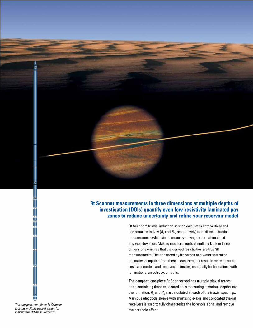
Rt Scanner* triaxial induction service calculates both vertical and horizontal resistivity (Rv and Rh, respectively) from direct induction measurements while simultaneously solving for formation dip at any well deviation. Making measurements at multiple DOIs in three dimensions ensures that the derived resistivities are true 3D measurements. The enhanced hydrocarbon and water saturation estimates computed from these measurements result in more accurate reservoir models and reserves estimates, especially for formations with laminations, anisotropy, or faults.

The compact, one-piece Rt Scanner tool has multiple triaxial arrays, each containing three collocated coils measuring at various depths into the formation. Rv and Rh are calculated at each of the triaxial spacings. A unique electrode sleeve with short single-axis and collocated triaxial receivers is used to fully characterize the borehole signal and remove the borehole effect.

Rt Scanner measurements in three dimensions at multiple depths of investigation (DOIs) quantify even low-resistivity laminated pay

zones to reduce uncertainty and refine your reservoir model

The compact, one-piece Rt Scanner tool has multiple triaxial arrays for making true 3D measurements.

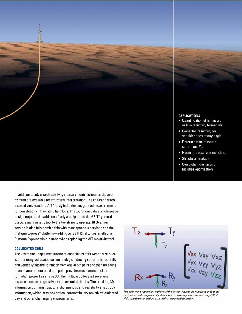
The collocated transmitter and one of the several collocated receivers (left) of the Rt Scanner tool independently obtain tensor resistivity measurements (right) that yield valuable information, especially in laminated formations.

In addition to advanced resistivity measurements, formation dip and azimuth are available for structural interpretation. The Rt Scanner tool also delivers standard AIT* array induction imager tool measurements for correlation with existing field logs. The tool’s innovative single-piece design requires the addition of only a caliper and the GPIT* general purpose inclinometry tool to the toolstring to operate. Rt Scanner service is also fully combinable with most openhole services and the Platform Express* platform—adding only 7 ft [2 m] to the length of a Platform Express triple-combo when replacing the AIT resistivity tool.

COLLOCATED COILS

The key to the unique measurement capabilities of Rt Scanner service is proprietary collocated coil technology. Inducing currents horizontally and vertically into the formation from one depth point and then receiving them at another mutual depth point provides measurement of the formation properties in true 3D. The multiple collocated receivers also measure at progressively deeper radial depths. The resulting 3D information contains structural dip, azimuth, and resistivity anisotropy information, which provides critical contrast in low-resistivity laminated pay and other challenging environments.

APPLICATIONS■ Quantification of laminated

or low-resistivity formations■ Corrected resistivity for

shoulder beds at any angle■ Determination of water

saturation, Sw

■ Geometric reservoir modeling■ Structural analysis■ Completion design and

facilities optimization

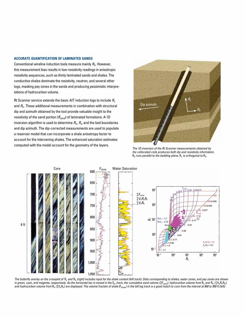
ACCURATE QUANTIFICATION OF LAMINATED SANDS

Conventional wireline induction tools measure mainly Rh. However, this measurement bias results in low-resistivity readings in anisotropic resistivity sequences, such as thinly laminated sands and shales. The conductive shales dominate the resistivity, neutron, and several other logs, masking pay zones in the sands and producing pessimistic interpre-tations of hydrocarbon volume.

Rt Scanner service extends the basic AIT induction logs to include Rv and Rh. These additional measurements in combination with structural dip and azimuth obtained by the tool provide valuable insight to the resistivity of the sand portion (Rsand) of laminated formations. A 1D inversion algorithm is used to determine Rh, Rv, and the bed boundaries and dip azimuth. The dip-corrected measurements are used to populate a reservoir model that can incorporate a shale anisotropy factor to account for the intervening shales. The enhanced saturation estimates computed with the model account for the geometry of the layers.

The 1D inversion of the Rt Scanner measurements obtained by the collocated coils produces both dip and resistivity information.Rh runs parallel to the bedding plane, Rv is orthogonal to Rh.

600

650

700

750

800

850

900

950

1,000

1,050

10–1

10–1 100 101

Rh

102 103

100

102

103

Core Fshale Water Saturation

R v 101

Fshale

Sw(RvRh) = 0.4Sw(Rh) = 0.87

∑Fsand

∑VhRvRh

∑VhRh

6 ft

Fshale

Rshv = 3.2Rshh = 0.56

Sw

Rsand

The butterfly overlay on the crossplot of Rv and Rh (right) includes input for the shale content (left track). Data corresponding to shales, water zones, and pay zones are shown in green, cyan, and magenta, respectively. As the horizontal bar is moved in the Sw track, the cumulative sand volume (∑Fsand), hydrocarbon volume from Rv and Rh (∑VhRvRh), and hydrocarbon volume from Rh (∑VhRh) are displayed. The volume fraction of shale (Fshale) in the left log track is a good match to core from the interval at 850 to 950 ft (left).

Dip azimuthRv

Rh

X,770

X,810

X,830

X,850

X,870

X,890

X,910

X,930

X,950

X,970

X,890

Y,010

Y,030

Y,050

Y,070

Y,090

Y,110

Y,130

X,790

Flowmeter Sw

Dry-WeightFraction

Depth,ft

Density 39-in Array Rh

ohm.m0.2 200

39-in Array Rv

ohm.m0.2 200

AIT 90 in

ohm.m0.2 200

ft3/ft3 g/cm31.65 2.65

Neutron Porosity

ft3/ft30.6 0

Total Sw

ft3/ft31 0

deg0 90

1 0

Shale

Sand

Density-NeutronCrossover

ELAN* Sw

FMI True DIP

Quality [4,12]Quality [12,120]

deg0 90

Triaxial AIT True DIPQuality [4,12]Quality [12,120]

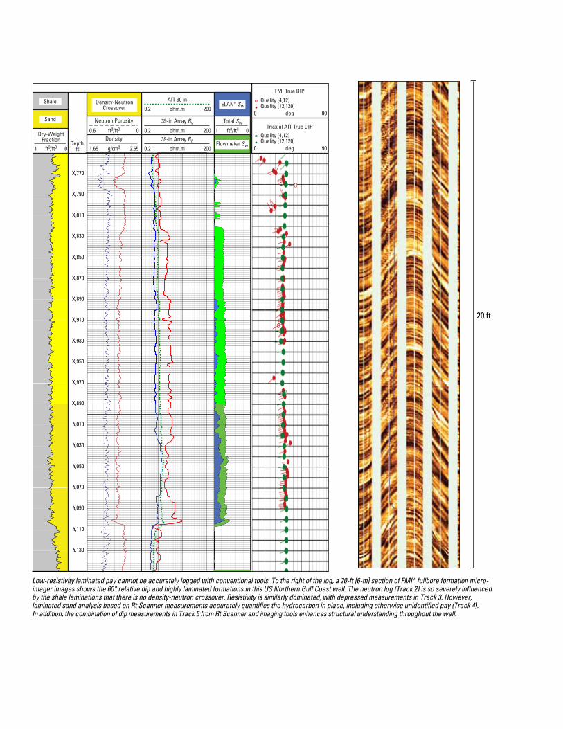
Low-resistivity laminated pay cannot be accurately logged with conventional tools. To the right of the log, a 20-ft [6-m] section of FMI* fullbore formation micro- imager images shows the 60° relative dip and highly laminated formations in this US Northern Gulf Coast well. The neutron log (Track 2) is so severely influenced by the shale laminations that there is no density-neutron crossover. Resistivity is similarly dominated, with depressed measurements in Track 3. However, laminated sand analysis based on Rt Scanner measurements accurately quantifies the hydrocarbon in place, including otherwise unidentified pay (Track 4). In addition, the combination of dip measurements in Track 5 from Rt Scanner and imaging tools enhances structural understanding throughout the well.

X,770

X,810

X,830

X,850

X,870

X,890

X,910

X,930

X,950

X,970

X,890

Y,010

Y,030

Y,050

Y,070

Y,090

Y,110

Y,130

X,790

Flowmeter Sw

Dry-WeightFraction

Depth,ft

Density 39-in Array Rh

ohm.m0.2 200

39-in Array Rv

ohm.m0.2 200

AIT 90 in

ohm.m0.2 200

ft3/ft3 g/cm31.65 2.65

Neutron Porosity

ft3/ft30.6 0

Total Sw

ft3/ft31 0

deg0 90

1 0

Shale

Sand

Density-NeutronCrossover

ELAN* Sw

FMI True DIP

Quality [4,12]Quality [12,120]

deg0 90

Triaxial AIT True DIPQuality [4,12]Quality [12,120]

20 ft

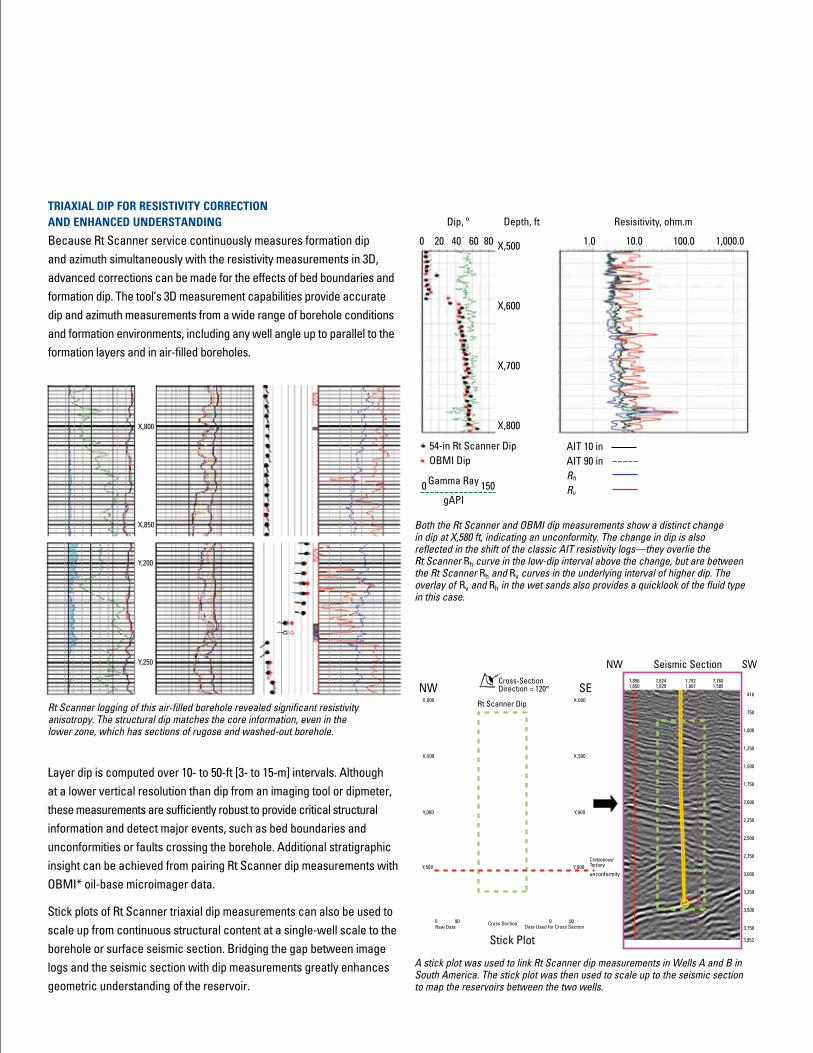
Both the Rt Scanner and OBMI dip measurements show a distinct change in dip at X,580 ft, indicating an unconformity. The change in dip is also reflected in the shift of the classic AIT resistivity logs—they overlie the Rt Scanner Rh curve in the low-dip interval above the change, but are between the Rt Scanner Rh and Rv curves in the underlying interval of higher dip. The overlay of Rv and Rh in the wet sands also provides a quicklook of the fluid type in this case.

Dip, º Depth, ft Resisitivity, ohm.m

0 20 40 60 80 X,500

X,600

X,700

X,800

1.0 10.0 100.0 1,000.0

54-in Rt Scanner Dip OBMI Dip

AIT 10 inAIT 90 inRh

Rv0 150

Gamma Ray

gAPI

TRIAXIAL DIP FOR RESISTIVITY CORRECTION AND ENHANCED UNDERSTANDING

Because Rt Scanner service continuously measures formation dip and azimuth simultaneously with the resistivity measurements in 3D, advanced corrections can be made for the effects of bed boundaries and formation dip. The tool’s 3D measurement capabilities provide accurate dip and azimuth measurements from a wide range of borehole conditions and formation environments, including any well angle up to parallel to the formation layers and in air-filled boreholes.

X,800

X,850

Y,200

Y,250

Rt Scanner logging of this air-filled borehole revealed significant resistivity anisotropy. The structural dip matches the core information, even in the lower zone, which has sections of rugose and washed-out borehole.

Layer dip is computed over 10- to 50-ft [3- to 15-m] intervals. Although at a lower vertical resolution than dip from an imaging tool or dipmeter, these measurements are sufficiently robust to provide critical structural information and detect major events, such as bed boundaries and unconformities or faults crossing the borehole. Additional stratigraphic insight can be achieved from pairing Rt Scanner dip measurements with OBMI* oil-base microimager data.

Stick plots of Rt Scanner triaxial dip measurements can also be used to scale up from continuous structural content at a single-well scale to the borehole or surface seismic section. Bridging the gap between image logs and the seismic section with dip measurements greatly enhances geometric understanding of the reservoir.

Rt Scanner Dip

Seismic SectionNW SW

X,000

X,500

Y,000

Y,500

X,000

X,500

Y,000

Y,500unconformity

7,8241,629

7,7921,607

7,7601,585

7,8561,650

416

750

1,000

1,250

1,500

1,750

2,000

2,250

2,500

2,750

3,000

3,250

3,500

3,750

3,952Stick Plot

NW SECross-SectionDirection = 120°

Raw Data0 90 0 90Cross Section

Data Used for Cross Section

Cretaceous/Tertiary

A stick plot was used to link Rt Scanner dip measurements in Wells A and B in South America. The stick plot was then used to scale up to the seismic section to map the reservoirs between the two wells.

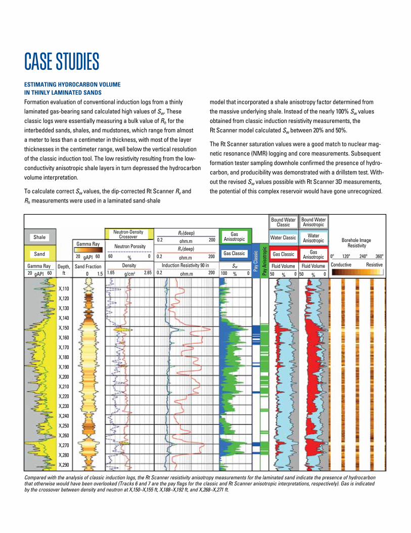
CASE STUDIESESTIMATING HYDROCARbON VOLUME IN THINLY LAMINATED SANDS

Formation evaluation of conventional induction logs from a thinly laminated gas-bearing sand calculated high values of Sw. These classic logs were essentially measuring a bulk value of Rh for the interbedded sands, shales, and mudstones, which range from almost a meter to less than a centimeter in thickness, with most of the layer thicknesses in the centimeter range, well below the vertical resolution of the classic induction tool. The low resistivity resulting from the low-conductivity anisotropic shale layers in turn depressed the hydrocarbon volume interpretation.

To calculate correct Sw values, the dip-corrected Rt Scanner Rv and Rh measurements were used in a laminated sand-shale

model that incorporated a shale anisotropy factor determined from the massive underlying shale. Instead of the nearly 100% Sw values obtained from classic induction resistivity measurements, the Rt Scanner model calculated Sw between 20% and 50%.

The Rt Scanner saturation values were a good match to nuclear mag-netic resonance (NMR) logging and core measurements. Subsequent formation tester sampling downhole confirmed the presence of hydro-carbon, and producibility was demonstrated with a drillstem test. With-out the revised Sw values possible with Rt Scanner 3D measurements, the potential of this complex reservoir would have gone unrecognized.

Shale

Sand

Gamma RaygAPI20 60

Depth,ft

Gamma Ray

gAPI20 60

Sand Fraction0 1.5

Neutron-Density Crossover

Neutron Porosity

60 0%Density

1.65 2.65g/cm3

Rh (deep)0.2 200ohm.m

0.2 200ohm.m

0.2 200ohm.m

Rv (deep)

Induction Resistivity 90 in

Gas Anisotropic

Gas Classic

%100 0Sw Pa

y Clas

sic

Pay A

nisot

ropic

Bound WaterClassic

Water Classic

Gas Classic

%50 0Fluid Volume

Bound WaterAnisotropic

Water Anisotropic

Gas Anisotropic

%50 0

Fluid Volume

0º 120º 240º 360º

Conductive Resistive

Borehole ImageResistivity

X,110

X,120

X,130

X,140

X,150

X,160

X,170

X,180

X,190

X,200

X,210

X,220

X,230

X,240

X,250

X,260

X,270

X,280

X,290

Compared with the analysis of classic induction logs, the Rt Scanner resistivity anisotropy measurements for the laminated sand indicate the presence of hydrocarbon that otherwise would have been overlooked (Tracks 6 and 7 are the pay flags for the classic and Rt Scanner anisotropic interpretations, respectively). Gas is indicated by the crossover between density and neutron at X,150–X,155 ft, X,188–X,192 ft, and X,268–X,271 ft.

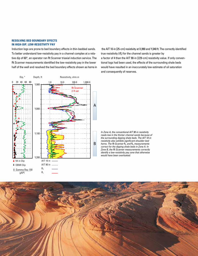
RESOLVING bED bOUNDARY EFFECTS IN HIGH-DIP, LOw-RESISTIVITY PAY

Induction logs are prone to bed boundary effects in thin-bedded sands. To better understand low-resistivity pay in a channel complex at a rela-tive dip of 60°, an operator ran Rt Scanner triaxial induction service. The Rt Scanner measurements identified the low-resistivity pay in the lower half of the well and resolved the bed boundary effects shown as horns in

the AIT 10-in [25-cm] resistivity at X,990 and Y,040 ft. The correctly identified true resistivity (Rt) for the channel sands is greater by a factor of 4 than the AIT 90-in [229-cm] resistivity value. If only conven-tional logs had been used, the effects of the surrounding shale beds would have resulted in an inaccurately low estimate of oil saturation and consequently of reserves.

Dip, º Depth, ft

0 20 40 60 80 1.0Y,900

Y,000

Y,100

Y,200

10.0 100.0

Rt Scanner2-ft set

1,000.0

Resisitivity, ohm.m

54-in Dip

OBMI Dip

0 150

Gamma RaygAPI

AIT 10 inAIT 90 inRh

Rv

A

B

In Zone A, the conventional AIT 90-in resistivity reads low in the thicker channel sands because of the surrounding dipping shale beds. The AIT 10-in resistivity also exhibits significant shoulder-bed horns. The Rt Scanner Rv and Rh measurements correct for the dipping shale beds in Zone A. In Zone B, the Rt Scanner measurements correctly identify a low-resistivity pay zone that otherwise would have been overlooked.

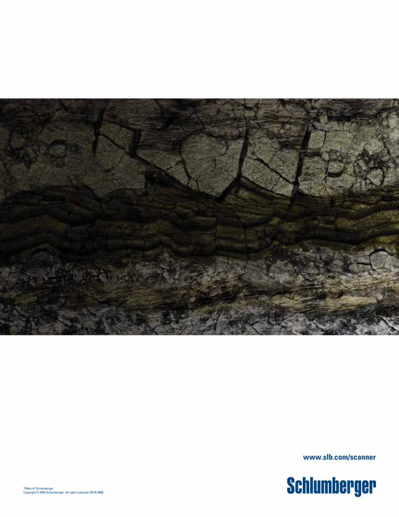
DRILLING A SUCCESSFUL DEEPwATER SIDETRACk IN THIN-bEDDED SANDS

Low-resistivity thin-bedded sands intercalated with shale layers were insufficiently characterized by conventional logs for placing a sidetrack in turbidite deposits offshore West Africa. Additional complications were the possible deformation of bedding by nearby salt deposits and that the seismic data was often doubtful because of the depth and seismic resolution.

To better understand this challenging situation, Schlumberger recommended dip angle measurements at multiple DOIs around the borehole well. The OBMI2* integrated dual oil-base microimagers and Rt Scanner triaxial induction service were run because they can obtain accurate images and measurements of low-resistivity formations drilled with oil-base mud. The OBMI2 tool recorded dip data around the borehole wall at a DOI of approximately 3.5 in [8.9 cm], and the Rt Scanner tool obtained far-field, radially variant dip measurements at DOIs of 39, 54, and 72 in [0.99, 13.7, and 1.8 m]. The Rt Scanner 3D dip measure-ment was also insensitive to any borehole irregularities, which were expected in this heterogeneous depositional environment.

Schlumberger Data & Consulting Services (DCS) introduced a improved approach to structural dip computation that integrated the two dip measurements. The first step was determining the level of confidence for the Rt Scanner dips with respect to borehole resistivity image dips from a known formation. The structural dip values were also compared with the vertical seismic profile to improve the view away from the borehole and better display large-scale variations in the deposits. The conventional averaging method was also used to compute another set of dip values for comparison.

The DCS analysis found that that as the DOI increases, the average dip decreases. The same bedding nature was also observed in the VSP data. Averaging the four sets of dip data achieved a more realistic structural dip value that could be used to improve reservoir modeling. With this information, the operator was able to drill a successful sidetrack.

New concept of computing structural dip

Formation

3.5 in39 in

54 in72 in

Bore

hole

�lle

d w

ith d

rillin

g m

ud

Rt Scanner

OBMI2

The new DCS concept for structural dip computation integrates dip measurements obtained at various DOIs. The green dots represent OBMI2 dips, and the red dots represent Rt Scanner multiarray dips. The green dotted line is a horizontal plane fitting the four-dip measurement.

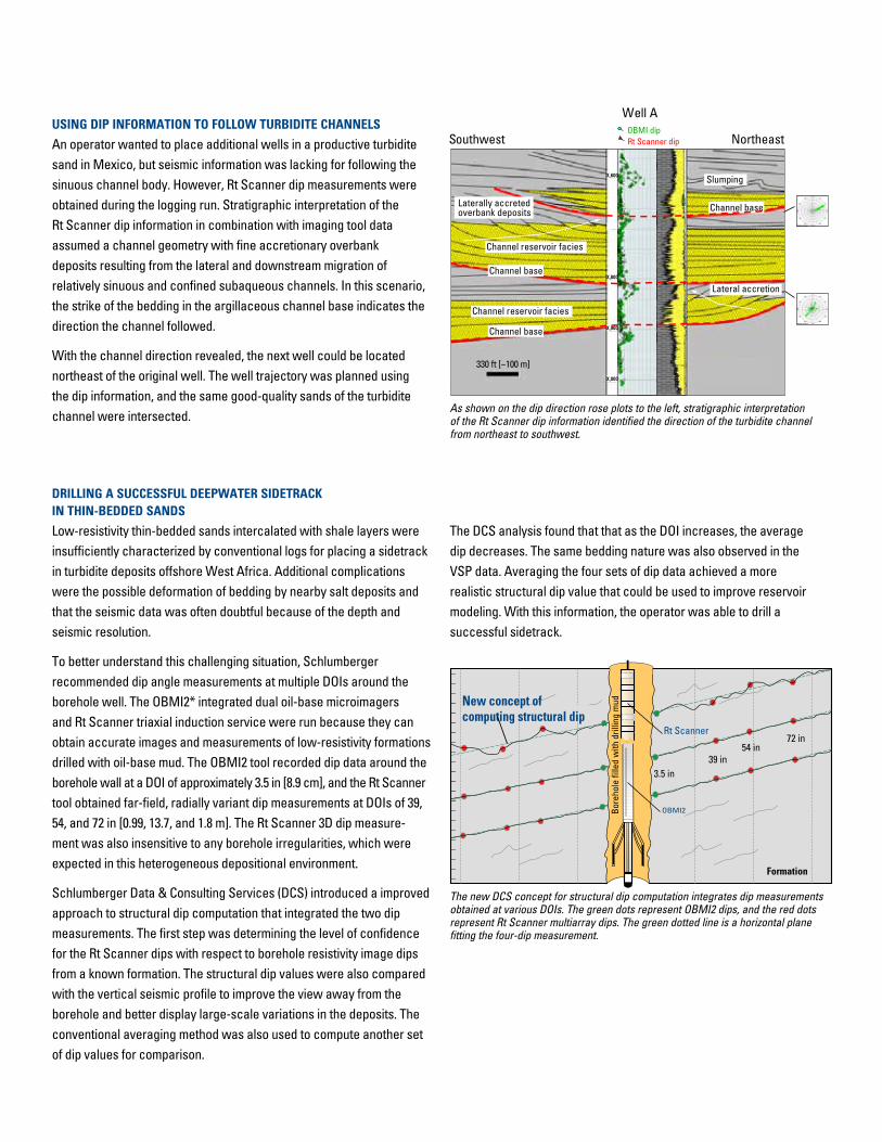
As shown on the dip direction rose plots to the left, stratigraphic interpretation of the Rt Scanner dip information identified the direction of the turbidite channel from northeast to southwest.

USING DIP INFORMATION TO FOLLOw TURbIDITE CHANNELS

An operator wanted to place additional wells in a productive turbidite sand in Mexico, but seismic information was lacking for following the sinuous channel body. However, Rt Scanner dip measurements were obtained during the logging run. Stratigraphic interpretation of the Rt Scanner dip information in combination with imaging tool data assumed a channel geometry with fine accretionary overbank deposits resulting from the lateral and downstream migration of relatively sinuous and confined subaqueous channels. In this scenario, the strike of the bedding in the argillaceous channel base indicates the direction the channel followed.

With the channel direction revealed, the next well could be located northeast of the original well. The well trajectory was planned using the dip information, and the same good-quality sands of the turbidite channel were intersected.

13/13/20073/13/2007

Well A

NortheastSouthwestOBMI dipRt Scanner dip

Lateral accretion

Channel reservoir facies

Channel reservoir facies

330 ft [~100 m]

X,600

X,800

X,000

X,900

Channel base

Channel base

Channel base

Slumping

Laterally accretedoverbank deposits

Specifications†

Output Rv, Rh, AIT logs, spontaneous potential, dip, azimuth

Max. logging speed 3,600 ft/h [1,097 m/h]Combinability Platform Express platform and most openhole servicesMax. temperature 302 degF [150 degC]Max. pressure 20,000 psi [137,895 kPa]

Bore hole size—min. 6 in [15.24 cm]Borehole size—max. 20 in [50.8 cm]Outside diameter 3.875 in [9.84 cm]Length‡ 19.6 ft [5.97 m]Weight 404 lbm [183 kg]Max. tension‡ 25,000 lbf [11,205 N]Max. compression§ 6,000 lbf [26,689 N] † A standoff is mandatory with this service ‡ GPIT tool is required to be run in combination § Limits derived at 302 degF and 0 psi

www.slb.com/scanner

*Mark of SchlumbergerCopyright © 2009 Schlumberger. All rights reserved. 09-FE-0008