tree-based batch mode reinforcement learning · tree-based batch mode reinforcement learning damien...
TRANSCRIPT
Journal of Machine Learning Research 6 (2005) 503–556 Submitted 11/03; Revised 4/04; Published 4/05
Tree-Based Batch Mode Reinforcement Learning
Damien Ernst [email protected]
Pierre Geurts [email protected]
Louis Wehenkel [email protected]
Department of Electrical Engineering and Computer ScienceInstitut Montefiore, University of LiegeSart-Tilman B28B4000 Liege, Belgium
Editor: Michael L. Littman
AbstractReinforcement learning aims to determine an optimal control policy from interaction with a systemor from observations gathered from a system. In batch mode, it can be achieved by approximatingthe so-calledQ-function based on a set of four-tuples(xt ,ut , rt ,xt+1) wherext denotes the sys-tem state at timet, ut the control action taken,rt the instantaneous reward obtained andxt+1 thesuccessor state of the system, and by determining the control policy from this Q-function. TheQ-function approximation may be obtained from the limit of a sequence of (batch mode) super-vised learning problems. Within this framework we describethe use of several classical tree-basedsupervised learning methods (CART, Kd-tree, tree bagging)and two newly proposed ensemble al-gorithms, namelyextremelyandtotally randomized trees. We study their performances on severalexamples and find that the ensemble methods based on regression trees perform well in extractingrelevant information about the optimal control policy fromsets of four-tuples. In particular, the to-tally randomized trees give good results while ensuring theconvergence of the sequence, whereasby relaxing the convergence constraint even better accuracy results are provided by the extremelyrandomized trees.
Keywords: batch mode reinforcement learning, regression trees, ensemble methods, supervisedlearning, fitted value iteration, optimal control
1. Introduction
Research in reinforcement learning (RL) aims at designing algorithms by which autonomous agentscan learn to behave in some appropriate fashion in some environment, from their interaction withthis environment or from observations gathered from the environment (see e.g. Kaelbling et al.(1996) or Sutton and Barto (1998) for a broad overview). The standard RL protocol considers aperformance agent operating in discrete time, observing at timet the environment statext , taking anactionut , and receiving back information from the environment (the next statext+1 and the instan-taneous rewardrt). After some finite time, the experience the agent has gathered from interactionwith the environment may thus be represented by a set of four-tuples(xt ,ut , rt ,xt+1).
In on-line learning the performance agent is also the learning agent whichat each time step canrevise its control policy with the objective of converging as quickly as possible to an optimal controlpolicy. In this paper we consider batch mode learning, where the learning agent is in principle notdirectly interacting with the system but receives only a set of four-tuples and is asked to determine
c©2005 Damien Ernst, Pierre Geurts and Louis Wehenkel.

ERNST, GEURTS AND WEHENKEL
from this set a control policy which is as close as possible to an optimal policy.Inspired by theon-lineQ-learning paradigm (Watkins, 1989), we will approach this batch mode learning problemby computing from the set of four-tuples an approximation of the so-calledQ-function defined onthe state-action space and by deriving from this latter function the control policy.
When the state and action spaces are finite and small enough, theQ-function can be representedin tabular form, and its approximation (in batch and in on-line mode) as well as thecontrol policyderivation are straightforward. However, when dealing with continuousor very large discrete stateand/or action spaces, theQ-function cannot be represented anymore by a table with one entry foreach state-action pair. Moreover, in the context of reinforcement learning an approximation of theQ-function all over the state-action space must be determined from finite and generally very sparsesets of four-tuples.
To overcome this generalization problem, a particularly attractive frameworkis the one used byOrmoneit and Sen (2002) which applies the idea of fitted value iteration (Gordon, 1999) to kernel-based reinforcement learning, and reformulates theQ-function determination problem as a sequenceof kernel-based regression problems. Actually, this framework makes it possible to take full advan-tage in the context of reinforcement learning of the generalization capabilities of any regressionalgorithm, and this contrary to stochastic approximation algorithms (Sutton, 1988; Tsitsiklis, 1994)which can only use parametric function approximators (for example, linear combinations of featurevectors or neural networks). In the rest of this paper we will call this framework thefitted Q iterationalgorithmso as to stress the fact that it allows to fit (using a set of four-tuples) any(parametric ornon-parametric) approximation architecture to theQ-function.
The fittedQ iteration algorithm is a batch mode reinforcement learning algorithm which yieldsan approximation of theQ-function corresponding to an infinite horizon optimal control problemwith discounted rewards, by iteratively extending the optimization horizon (Ernst et al., 2003):
• At the first iteration it produces an approximation of aQ1-function corresponding to a 1-stepoptimization. Since the trueQ1-function is the conditional expectation of the instantaneousreward given the state-action pair (i.e.,Q1(x,u) = E[rt |xt = x,ut = u]), an approximation ofit can be constructed by applying a (batch mode) regression algorithm to a training set whoseinputs are the pairs(xt ,ut) and whose target output values are the instantaneous rewardsrt
(i.e.,q1,t = rt).
• The Nth iteration derives (using a batch mode regression algorithm) an approximation of aQN-function corresponding to anN-step optimization horizon. The training set at this stepis obtained by merely refreshing the output values of the training set of the previous step byusing the “value iteration” based on the approximateQN-function returned at the previousstep (i.e.,qN,t = rt + γmaxuQN−1(xt+1,u), whereγ ∈ [0,1) is the discount factor).
Ormoneit and Sen (2002) have studied the theoretical convergence andconsistency properties ofthis algorithm when combined with kernel-based regressors. In this paper, we study within thisframework the empirical properties and performances of several tree-based regression algorithmson several applications. Just like kernel-based methods, tree-based methods are non-parametricand offer a great modeling flexibility, which is a paramount characteristic for the framework to besuccessful since the regression algorithm must be able to model anyQN-function of the sequence,functions which are a priori totally unpredictable in shape. But, from a practical point of view thesetree-based methods have a priori some additional advantages, such as their high computational
504
TREE-BASED BATCH MODE REINFORCEMENTLEARNING
efficiency and scalability to high-dimensional spaces, their fully autonomouscharacter, and theirrecognized robustness to irrelevant variables, outliers, and noise.
In addition to good accuracy when trained with finite sets of four-tuples, one desirable feature ofthe regression method used in the context of the fittedQ iteration algorithm is to ensure convergenceof the sequence. We will analyze under which conditions the tree-based methods share this propertyand also what is the relation between convergence and quality of approximation. In particular, wewill see that ensembles of totally randomized trees (i.e., trees built by selecting their splits randomly)can be adapted to ensure the convergence of the sequence while leadingto good approximationperformances. On the other hand, another tree-based algorithm named extremely randomized trees(Geurts et al., 2004), will be found to perform consistently better than totallyrandomized trees eventhough it does not strictly ensure the convergence of the sequence ofQ-function approximations.
The remainder of this paper is organized as follows. In Section 2, we formalize the reinforce-ment learning problem considered here and recall some classical resultsfrom optimal control theoryupon which the approach is based. In Section 3 we present thefitted Q iteration algorithmand inSection 4 we describe the different tree-based regression methods considered in our empirical tests.Section 5 is dedicated to the experiments where we apply the fittedQ iteration algorithm used withtree-based methods to several control problems with continuous state spaces and evaluate its perfor-mances in a wide range of conditions. Section 6 concludes and also provides our main directions forfurther research. Three appendices collect relevant details about algorithms, mathematical proofsand benchmark control problems.
2. Problem Formulation and Dynamic Programming
We consider a time-invariant stochastic system in discrete time for which a closed loop stationarycontrol policy1 must be chosen in order to maximize an expected discounted return over an infinitetime horizon. We formulate hereafter the batch mode reinforcement learning problem in this contextand we restate some classical results stemming from Bellman’s dynamic programming approach tooptimal control theory (introduced in Bellman, 1957) and from which the fittedQ iteration algorithmtakes its roots.
2.1 Batch Mode Reinforcement Learning Problem Formulation
Let us consider a system having adiscrete-time dynamicsdescribed by
xt+1 = f (xt ,ut ,wt) t = 0,1, · · · , (1)
where for allt, the statext is an element of the state spaceX, the actionut is an element of the actionspaceU and the random disturbancewt an element of the disturbance spaceW. The disturbancewt
is generated by the time-invariant conditional probability distributionPw(w|x,u).2
To the transition fromt to t + 1 is associated an instantaneousreward signal rt = r(xt ,ut ,wt)wherer(x,u,w) is the reward function supposed to be bounded by some constantBr .
Let µ(·) : X → U denote a stationary control policy andJµ∞ denote the expected return ob-
tained over an infinite time horizon when the system is controlled using this policy (i.e., when
1. Indeed, in terms of optimality this restricted family of control policies is as good as the broader set of all non-anticipating (and possibly time-variant) control policies.
2. In other words, the probabilityP(wt = w|xt = x,ut = u) of occurrence ofwt = w given that the current statext andthe current controlut arex andu respectively, is equal toPw(w|x,u),∀t = 0,1, · · · .
505
ERNST, GEURTS AND WEHENKEL
ut = µ(xt),∀t). For a given initial conditionx0 = x, Jµ∞ is defined by
Jµ∞(x) = lim
N→∞Ewt
t=0,1,··· ,N−1
[N−1
∑t=0
γtr(xt ,µ(xt),wt)|x0 = x], (2)
whereγ is a discount factor (0≤ γ < 1) that weights short-term rewards more than long-term ones,and where the conditional expectation is taken over all trajectories starting with the initial condi-tion x0 = x. Our objective is to find an optimal stationary policyµ∗, i.e. a stationary policy thatmaximizesJµ
∞ for all x.The existence of an optimal stationary closed loop policy is a classical resultfrom dynamic
programming theory. It could be determined in principle by solving the Bellman equation (seebelow, Eqn (6)) given the knowledge of the system dynamics and rewardfunction. However, the soleinformation that we assume available to solve the problem is the one obtained from the observationof a certain number of one-step system transitions (fromt to t +1). Each system transition providesthe knowledge of a new four-tuple(xt ,ut , rt ,xt+1) of information. Since, except for very specialconditions, it is not possible to determine exactly an optimal control policy froma finite sample ofsuch transitions, we aim at computing an approximation of such aµ∗ from a set
F = {(xlt ,u
lt , r
lt ,x
lt+1), l = 1, · · · ,#F }
of such four-tuples.We do not make any particular assumptions on the way the set of four-tuplesis generated. It
could be generated by gathering the four-tuples corresponding to one single trajectory (or episode)as well as by considering several independently generated one or multi-step episodes.
We call this problem thebatch modereinforcement learning problem because the algorithm isallowed to use a set of transitions of arbitrary size to produce its control policy in a single step. Incontrast, anon-linealgorithm would produce a sequence of policies corresponding to a sequence offour-tuples.
2.2 Results from Dynamic Programming Theory
For a temporal horizon ofN steps, let us denote by
πN(t,x) ∈U, t ∈ {0, · · · ,N−1};x∈ X
a (possibly time-varying)N-step control policy (i.e.,ut = πN(t,xt) ), and by
JπNN (x) = E
wtt=0,1,··· ,N−1
[N−1
∑t=0
γtr(xt ,πN(t,xt),wt)|x0 = x] (3)
its expected return overN steps. AnN-step optimal policyπ∗N is a policy which among all possiblesuch policies maximizesJπN
N for anyx. Notice that under mild conditions (see e.g. Hernandez-Lermaand Lasserre, 1996, for the detailed conditions) such a policy always does indeed exist although itis not necessarily unique.
Our algorithm exploits the following classical results from dynamic programmingtheory (Bell-man, 1957):
506

TREE-BASED BATCH MODE REINFORCEMENTLEARNING
1. The sequence ofQN-functions defined onX×U by
Q0(x,u) ≡ 0 (4)
QN(x,u) = (HQN−1)(x,u), ∀N > 0, (5)
converges (in infinity norm) to theQ-function, defined as the (unique) solution of the Bellmanequation:
Q(x,u) = (HQ)(x,u) (6)
whereH is an operator mapping any functionK : X×U → R and defined as follows:3
(HK)(x,u) = Ew[r(x,u,w)+ γmax
u′∈UK( f (x,u,w),u′)]. (7)
Uniqueness of solution of Eqn (6) as well as convergence of the sequence ofQN-functionsto this solution are direct consequences of the fixed point theorem and ofthe fact thatH is acontraction mapping.
2. The sequence of policies defined by the two conditions4
π∗N(0,x) = argmaxu′∈U
QN(x,u′),∀N > 0 (8)
π∗N(t +1,x) = π∗N−1(t,x),∀N > 1, t ∈ {0, . . . ,N−2} (9)
areN-step optimal policies, and their expected returns overN steps are given by
Jπ∗NN (x) = max
u∈UQN(x,u).
3. A policy µ∗ that satisfiesµ∗(x) = argmax
u∈UQ(x,u) (10)
is an optimal stationary policy for the infinite horizon case and the expected return ofµ∗N(x).=
π∗N(0,x) converges to the expected return ofµ∗:
limN→∞
Jµ∗N∞ (x) = Jµ∗
∞ (x) ∀x∈ X. (11)
We have also limN→∞ Jπ∗NN (x) = Jµ∗
∞ (x) ∀x∈ X.
Equation (5) defines the so-calledvalue iteration algorithm5 providing a way to determine iter-atively a sequence of functions converging to theQ-function and hence of policies whose returnconverges to that of an optimal stationary policy, assuming that the system dynamics, the rewardfunction and the noise distribution are known. As we will see in the next section, it suggests also away to determine approximations of theseQN-functions and policies from a sampleF .
3. The expectation is computed by usingP(w) = Pw(w|x,u).4. Actually this definition does not necessarily yield a unique policy, but anypolicy which satisfies these conditions is
appropriate.
5. Strictly, the term “value iteration” refers to the computation of thevaluefunctionJµ∗∞ and corresponds to the iteration
Jπ∗NN = max
u∈UEw[r(x,u,w)+ γJ
π∗N−1N−1( f (x,u,w))],∀N > 0 rather than Eqn (5).
507

ERNST, GEURTS AND WEHENKEL
3. Fitted Q Iteration Algorithm
In this section, we introduce the fittedQ iteration algorithm which computes from a set of four-tuples an approximation of the optimal stationary policy.
3.1 The Algorithm
A tabular version of the fittedQ iteration algorithm is given in Figure 1. At each step this algorithmmay use the full set of four-tuples gathered from observation of the system together with the functioncomputed at the previous step to determine a new training set which is used by asupervised learning(regression) method to compute the next function of the sequence. It produces a sequence ofQN-functions, approximations of theQN-functions defined by Eqn (5).
Inputs: a set of four-tuplesF and a regression algorithm.Initialization:SetN to 0 .Let QN be a function equal to zero everywhere onX×U .Iterations:Repeat until stopping conditions are reached
- N← N+1 .
- Build the training setT S = {(i l ,ol ), l = 1, · · · ,#F } based on the the functionQN−1 and onthe full set of four-tuplesF :
i l = (xlt ,u
lt) , (12)
ol = r lt + γmax
u∈UQN−1(x
lt+1,u) . (13)
- Use the regression algorithm to induce fromT S the functionQN(x,u).
Figure 1: FittedQ iteration algorithm
Notice that at the first iteration the fittedQ iteration algorithm is used in order to produce anapproximation of the expected rewardQ1(x,u) = Ew[r(x,u,w)]. Therefore, the considered trainingset uses input/output pairs (denoted(i l ,ol )) where the inputs are the state-action pairs and the outputsthe observed rewards. In the subsequent iterations, only the output values of these input/output pairsare updated using the value iteration based on theQN-function produced at the preceding step andinformation about the reward and the successor state reached in each tuple.
It is important to realize that the successive calls to the supervised learningalgorithm are totallyindependent. Hence, at each step it is possible to adapt the resolution (orcomplexity) of the learnedmodel so as to reach the best bias/variance tradeoff at this step, given the available sample.
3.2 Algorithm Motivation
To motivate the algorithm, let us first consider the deterministic case. In this case the system dy-namics and the reward signal depend only on the state and action at timet. In other words we have
508

TREE-BASED BATCH MODE REINFORCEMENTLEARNING
xt+1 = f (xt ,ut) andrt = r(xt ,ut) and Eqn (5) may be rewritten
QN(x,u) = r(x,u)+ γmaxu′∈U
QN−1( f (x,u),u′). (14)
If we suppose that the functionQN−1 is known, we can use this latter equation and the set of four-tuplesF in order to determine the value ofQN for the state-action pairs(xl
t ,ult), l = 1,2, · · · ,#F .
We have indeedQN(xlt ,u
lt) = r l
t + γmaxu′∈U
QN−1(xlt+1,u
′), sincexlt+1 = f (xl
t ,ult) andr l
t = r(xlt ,u
lt).
We can thus build a training setT S = {((xlt ,u
lt),QN(xl
t ,ult)), l = 1, · · · ,#F } and use a regression
algorithm in order to generalize this information to any unseen state-action pairor, stated in anotherway, tofit a function approximator to this training set in order to get an approximationQN of QN overthe whole state-action space. If we substituteQN for QN we can, by applying the same reasoning,determine iterativelyQN+1, QN+2, etc.
In the stochastic case, the evaluation of the right hand side of Eqn (14) for some four-tuples(xt ,ut , rt ,xt+1) is no longer equal toQN(xt ,ut) but rather is the realization of a random variablewhose expectation isQN(xt ,ut). Nevertheless, since a regression algorithm usually6 seeks an ap-proximation of the conditional expectation of the output variable given the inputs, its applicationto the training setT S will still provide an approximation ofQN(x,u) over the whole state-actionspace.
3.3 Stopping Conditions
The stopping conditions are required to decide at which iteration (i.e., for which value ofN) theprocess can be stopped. A simple way to stop the process is to define a priori a maximum numberof iterations. This can be done for example by noting that for a sequence of optimal policiesµ∗N, anerror bound on the sub-optimality in terms of number of iterations is given by thefollowing equation
‖Jµ∗N∞ −Jµ∗∞ ‖∞ ≤ 2
γNBr
(1− γ)2 . (15)
Given the value ofBr and a desired level of accuracy, one can then fix the maximum number ofiterations by computing the minimum value ofN such that the right hand side of this equation issmaller than the tolerance fixed.7
Another possibility would be to stop the iterative process when the distance betweenQN andQN−1 drops below a certain value. Unfortunately, for some supervised learning algorithms there isno guarantee that the sequence ofQN-functions actually converges and hence this kind of conver-gence criterion does not necessarily make sense in practice.
3.4 Control Policy Derivation
When the stopping conditions - whatever they are - are reached, the finalcontrol policy, seen as anapproximation of the optimal stationary closed loop control policy is derived by
µ∗N(x) = argmaxu∈U
QN(x,u). (16)
6. This is true in the case of least squares regression, i.e. in the vast majority of regression methods.7. Equation (15) gives an upper bound on the suboptimality ofµ∗N and not ofµ∗N. By exploiting this upper bound
to determine a maximum number of iterations, we assume implicitly that ˆµ∗N is a good approximation ofµ∗N (that
‖Jµ∗N∞ −Jµ∗N∞ ‖∞ is small).
509
ERNST, GEURTS AND WEHENKEL
When the action space is discrete, it is possible to compute the valueQN(x,u) for each valueof u and then find the maximum. Nevertheless, in our experiments we have sometimes adopteda different approach to handle discrete action spaces. It consists of splitting the training samplesaccording to the value ofu and of building the approximationQN(x,u) by separately calling foreach value ofu∈U the regression method on the corresponding subsample. In other words,eachsuch model is induced from the subset of four-tuples whose value of theaction isu, i.e.
Fu = {(xt ,ut , rt ,xt+1) ∈ F |ut = u}.
At the end, the action at some pointx of the state space is computed by applying to this state eachmodelQN(x,u),u∈U and looking for the value ofu yielding the highest value.
When the action space is continuous, it may be difficult to compute the maximum especiallybecause we can not make any a priori assumption about the shape of theQ-function (e.g. convex-ity). However, taking into account particularities of the models learned by a particular supervisedlearning method, it may be more or less easy to compute this value (see Section 4.5for the case oftree-based models).
3.5 Convergence of the FittedQ Iteration Algorithm
The fittedQ iteration algorithm is said to converge if there exists a functionQ : X×U → R suchthat∀ε > 0 there exists an∈ N such that:
‖QN− Q‖∞ < ε ∀N > n.
Convergence may be ensured if we use a supervised learning method which given a sampleT S ={(i1,o1), . . . ,(i#T S ,o#T S )} produces at each call the model (proof in Appendix B):
f (i) =#T S
∑l=1
kT S (i l , i)∗ol, (17)
with the kernelkT S (i l , i) being the same from one call to the other within the fittedQ iterationalgorithm8 and satisfying the normalizing condition:
#T S
∑l=1
|kT S (i l , i)|= 1, ∀i. (18)
Supervised learning methods satisfying these conditions are for example thek-nearest-neighborsmethod, partition and multi-partition methods, locally weighted averaging, linear, and multi-linearinterpolation. They are collectively referred to as kernel-based methods(see Gordon, 1999; Or-moneit and Sen, 2002).
3.6 Related Work
As stated in the Introduction, the idea of trying to approximate theQ-function from a set of four-tuples by solving a sequence of supervised learning problems may alreadybe found in Ormoneit and
8. This is true when the kernel does not depend on the output values of the training sample and when the supervisedlearning method is deterministic.
510

TREE-BASED BATCH MODE REINFORCEMENTLEARNING
Sen (2002). This work however focuses on kernel-based methods for which it provides convergenceand consistency proofs, as well as a bias-variance characterization.While in our formulation stateand action spaces are handled in a symmetric way and may both be continuous or discrete, in theirwork Ormoneit and Sen consider only discrete action spaces and use a separate kernel for each valueof the action.
The work of Ormoneit and Sen is related to earlier work aimed to solve large-scale dynamic pro-gramming problems (see for example Bellman et al., 1973; Gordon, 1995b; Tsitsiklis and Van Roy,1996; Rust, 1997). The main difference is that in these works the variouselements that composethe optimal control problem are supposed to be known. We gave the namefitted Q iterationto ouralgorithm given in Figure 1 to emphasize that it is a reinforcement learning version of thefittedvalue iterationalgorithm whose description may be found in Gordon (1999). Both algorithms arequite similar except that Gordon supposes that a complete generative model isavailable,9 which isa rather strong restriction with respect to the assumptions of the present paper.
In his work, Gordon characterizes a class of supervised learning methods referred to as averagersthat lead to convergence of his algorithm. These averagers are in fact aparticular family of kernelsas considered by Ormoneit and Sen. In Boyan and Moore (1995), serious convergence problemsthat may plague the fitted value iteration algorithm when used with polynomial regression, back-propagation, or locally weighted regression are shown and these also apply to the reinforcementlearning context. In their paper, Boyan and Moore propose also a way toovercome this problemby relying on some kind of Monte-Carlo simulations. In Gordon (1995a) andSingh et al. (1995)on-line versions of the fitted value iteration algorithm used with averagers are presented.
In Moore and Atkeson (1993) and Ernst (2003), several reinforcement learning algorithmsclosely related to the fittedQ iteration algorithm are given. These algorithms, known as model-based algorithms, build explicitly from the set of observations a finite MarkovDecision Process(MDP) whose solution is then used to adjust the parameters of the approximation architecture usedto represent theQ-function. When the states of the MDP correspond to a finite partition of theoriginal state space, it can be shown that these methods are strictly equivalent to using the fittedQiteration algorithm with a regression method which consists of simply averaging the output valuesof the training samples belonging to a given cell of the partition.
In Boyan (2002), the Least-Squares Temporal-Difference (LSTD) algorithm is proposed. Thisalgorithm uses linear approximation architectures and learns the expected return of a policy. It issimilar to the fittedQ iteration algorithm combined with linear regression techniques on problemsfor which the action space is composed of a single element. Lagoudakis and Parr (2003a) intro-duce the Least-Squares Policy Iteration (LSPI) which is an extension of LSTD to control problems.The model-based algorithms in Ernst (2003) that consider representative states as approximationarchitecture may equally be seen as an extension of LSTD to control problems.
Finally, we would like to mention some recent works based on the idea of reductions of rein-forcement learning to supervised learning (classification or regression) with various assumptionsconcerning the available a priori knowledge (see e.g. Kakade and Langford, 2002; Langford andZadrozny, 2004, and the references therein). For example, assumingthat a generative model isavailable,10 an approach to solve the optimal control problem by reformulating it as a sequence of
9. Gordon supposes that the functionsf (·, ·, ·), r(·, ·, ·), andPw(·|·, ·) are known and considers training sets composed of
elements of the type(x,maxu∈U
Ew[r(x,u,w)+ γJ
π∗N−1N−1( f (x,u,w))]).
10. A generative model allows simulating the effect of any action on the system at any starting point; this is less restrictivethan thecompletegenerative model assumption of Gordon (footnote 9, page 511).
511

ERNST, GEURTS AND WEHENKEL
standard supervised classification problems has been developed (see Lagoudakis and Parr, 2003b;Bagnell et al., 2003), taking its roots from the policy iteration algorithm, another classical dynamicprogramming algorithm. Within this “reductionist” framework, the fittedQ iteration algorithm canbe considered as areductionof reinforcement learning to a sequence of regression tasks, inspiredbythe value iteration algorithm and usable in the rather broad context where theavailable informationis given in the form of a set of four-tuples. Thisbatch modecontext incorporates indeed both theon-line context (since one can always store data gathered on-line, at least for a finite time interval) aswell as the generative context (since one can always use the generative model to generate a sampleof four-tuples) as particular cases.
4. Tree-Based Methods
We will consider in our experiments five different tree-based methods all based on the same top-down approach as in the classical tree induction algorithm. Some of these methods will producefrom the training set a model composed of onesingleregression tree while the others build anen-sembleof regression trees. We characterize first the models that will be produced by these tree-basedmethods and then explain how the different tree-based methods generate these models. Finally, wewill consider some specific aspects related to the use of tree-based methods with the fittedQ itera-tion algorithm.
4.1 Characterization of the Models Produced
A regression tree partitions the input space into several regions and determines a constant predictionin each region of the partition by averaging the output values of the elements of the training setT S
which belong to this region. LetS(i) be the function that assigns to an inputi (i.e., a state-action pair)the region of the partition it belongs to. A regression tree produces a modelthat can be describedby Eqn (17) with the kernel defined by the expression:
kT S (i l , i) =IS(i)(i
l )
∑(a,b)∈T S IS(i)(a)(19)
whereIB(·) denotes the characteristic function of the regionB (IB(i) = 1 if i ∈ B and 0 otherwise).When a tree-based method builds an ensemble of regression trees, the model it produces av-
erages the predictions of the different regression trees to make a final prediction. Suppose that atree-based ensemble method producesp regression trees and gets as input a training setT S . LetT Sm
11 be the training set used to build themth regression tree (and therefore themth partition) andSm(i) be the function that assigns to eachi the region of themth partition it belongs to. The modelproduced by the tree-based method may also be described by Eqn (17) withthe kernel defined nowby the expression:
kT S (i l , i) =1p
p
∑m=1
ISm(i)(il )
∑(a,b)∈T SmISm(i)(a)
. (20)
It should also be noticed that kernels (19) and (20) satisfy the normalizingcondition (18).
11. These subsets may be obtained in different ways from the original training set, e.g. by sampling with or withoutreplacement, but we can assume that each element ofT Sm is also an element ofT S .
512

TREE-BASED BATCH MODE REINFORCEMENTLEARNING
4.2 The Different Tree-Based Algorithms
All the tree induction algorithms that we consider are top-down in the sense that they create theirpartition by starting with a single subset and progressively refining it by splitting its subsets intopieces. The tree-based algorithms that we consider differ by the number of regression trees theybuild (one or an ensemble), the way they grow a tree from a training set (i.e.,the way the differenttests inside the tree are chosen) and, in the case of methods that produce an ensemble of regressiontrees, also the way they derive from the original training setT S the training setT Sm they use tobuild a particular tree. They all consider binary splits of the type[i j < t], i.e. “if i j smaller thant goleft else go right” wherei j represents thejth input (or jth attribute) of the input vectori. In whatfollows the split variablest andi j are referred to as the cut-point and the cut-direction (or attribute)of the split (or test)[i j < t].
We now describe the tree-based regression algorithms used in this paper.
4.2.1 KD-TREE
In this method the regression tree is built from the training set by choosing thecut-point at the localmedian of the cut-direction so that the tree partitions the local training set into twosubsets of thesame cardinality. The cut-directions alternate from one node to the other: if the direction of cut isi j for the parent node, it is equal toi j+1 for the two children nodes ifj +1 < n with n the numberof possible cut-directions andi1 otherwise. A node is a leaf (i.e., is not partitioned) if the trainingsample corresponding to this node contains less thannmin tuples. In this method the tree structure isindependent of the output values of the training sample, i.e. it does not change from one iteration toanother of the fittedQ iteration algorithm.
4.2.2 PRUNED CART TREE
The classical CART algorithm is used to grow completely the tree from the training set (Breimanet al., 1984). This algorithm selects at a node the test (i.e., the cut-direction and cut-point) thatmaximizes the average variance reduction of the output variable (see Eqn (25) in Appendix A). Thetree is pruned according to the cost-complexity pruning algorithm with error estimate by ten-foldcross validation. Because of the score maximization and the post-pruning, the tree structure dependson the output values of the training sample; hence, it may change from one iteration to another.
4.2.3 TREE BAGGING
We refer here to the standard algorithm published by Breiman (1996). An ensemble ofM trees isbuilt. Each tree of the ensemble is grown from a training set by first creatinga bootstrap replica(random sampling with replacement of the same number of elements) of the training set and thenbuilding an unpruned CART tree using that replica. Compared to the PrunedCART Tree algorithm,Tree Bagging often improves dramatically the accuracy of the model produced by reducing itsvariance but increases the computing times significantly. Note that during the tree building we alsostop splitting a node if the number of training samples in this node is less thannmin. This algorithmhas therefore two parameters, the numberM of trees to build and the value ofnmin.
513

ERNST, GEURTS AND WEHENKEL
One single
regression tree is built
An ensemble of
regression trees is built
Testsdo dependon the output
values (o) of the(i,o) ∈ T SCART
Tree Bagging
Extra-Trees
Testsdo not dependon the output
values (o) of the(i,o) ∈ T SKd-Tree Totally Randomized Trees
Table 1: Main characteristics of the different tree-based algorithms usedin the experiments.
4.2.4 EXTRA-TREES
Besides Tree Bagging, several other methods to build tree ensembles havebeen proposed that oftenimprove the accuracy with respect to Tree Bagging (e.g. Random Forests, Breiman, 2001). Inthis paper, we evaluate our recently developed algorithm that we call “Extra-Trees”, for extremelyrandomized trees (Geurts et al., 2004). Like Tree Bagging, this algorithm works by building several(M) trees. However, contrary to Tree Bagging which uses the standard CART algorithm to derivethe trees from a bootstrap sample, in the case of Extra-Trees, each tree isbuilt from the completeoriginal training set. To determine a test at a node, this algorithm selectsK cut-directions at randomand for each cut-direction, a cut-point at random. It then computes a score for each of theK tests andchooses among theseK tests the one that maximizes the score. Again, the algorithm stops splittinga node when the number of elements in this node is less than a parameternmin. Three parameters areassociated to this algorithm: the numberM of trees to build, the numberK of candidate tests at eachnode and the minimal leaf sizenmin. The detailed tree building procedure is given in Appendix A.
4.2.5 TOTALLY RANDOMIZED TREES
Totally Randomized Trees corresponds to the case of Extra-Trees whenthe parameterK is chosenequal to one. Indeed, in this case the tests at the different nodes are chosen totally randomly andindependently from the output values of the elements of the training set. Actually, this algorithm isequivalent to an algorithm that would build the tree structure totally at randomwithout even lookingat the training set and then use the training set only to remove the tests that leadto empty branchesand decide when to stop the development of a branch (Geurts et al., 2004). This algorithm cantherefore be degenerated in the context of the usage that we make of it in this paper by freezing thetree structure after the first iteration, just as the Kd-Trees.
4.2.6 DISCUSSION
Table 1 classifies the different tree-based algorithms considered according to two criteria: whetherthey build one single or an ensemble of regression trees and whether the tests computed in the treesdepend on the output values of the elements of the training set. We will see in theexperiments thatthese two criteria often characterize the results obtained.
Concerning the value of parameterM (the number of trees to be built) we will use the samevalue for Tree Bagging, Extra-Trees and Totally Randomized Trees andset it equal to 50 (except inSection 5.3.6 where we will assess its influence on the solution computed).
514

TREE-BASED BATCH MODE REINFORCEMENTLEARNING
For the Extra-Trees, experiments in Geurts et al. (2004) have shown that a good default value forthe parameterK in regression is actually the dimension of the input space. In all our experiments,K will be set to this default value.
While pruning generally improves significantly the accuracy of single regression trees, in thecontext of ensemble methods it is commonly admitted that unpruned trees are better. This is sug-gested from the bias/variance tradeoff, more specifically because pruning reduces variance but in-creases bias and since ensemble methods reduce very much the variance without increasing toomuch bias, there is often no need for pruning trees in the context of ensemble methods. However, inhigh-noise conditions, pruning may be useful even with ensemble methods. Therefore, we will usea cross-validation approach to automatically determine the value ofnmin in the context of ensemblemethods. In this case, pruning is carried out by selecting at random two thirds of the elements ofT S , using the particular ensemble method with this smaller training set and determining for whichvalue ofnmin the ensemble minimizes the square error over the last third of the elements. Then,the ensemble method is run again on the whole training set using this value ofnmin to produce thefinal model. In our experiments, the resulting algorithm will have the same name as the originalensemble method preceded by the termPruned(e.g. Pruned Tree Bagging). The same approachwill also be used to prune Kd-Trees.
4.3 Convergence of the FittedQ Iteration Algorithm
Since the models produced by the tree-based methods may be described by an expression of the type(17) with the kernelkT S (i l , i) satisfying the normalizing condition (18), convergence of the fittedQiteration algorithm can be ensured if the kernelkT S (i l , i) remains the same from one iteration to theother. This latter condition is satisfied when the tree structures remain unchanged throughout thedifferent iterations.
For the Kd-Tree algorithm which selects tests independently of the output values of the elementsof the training set, it can be readily seen that it will produce at each iterationthe same tree structureif the minimum number of elements to split a leaf (nmin) is kept constant. This also implies that thetree structure has just to be built at the first iteration and that in the subsequent iterations, only thevalues of the terminal leaves have to be refreshed. Refreshment may be done by propagating all theelements of the new training set in the tree structure and associating to a terminalleaf the averageoutput value of the elements having reached this leaf.
For the totally randomized trees, the tests do not depend either on the output values of theelements of the training set but the algorithm being non-deterministic, it will not produce the sametree structures at each call even if the training set and the minimum number of elements (nmin) tosplit a leaf are kept constant. However, since the tree structures are independent from the output, itis not necessary to refresh them from one iteration to the other. Hence, inour experiments, we willbuild the set of totally randomized trees only at the first iteration and then only refresh predictionsat terminal nodes at subsequent iterations. The tree structures are therefore kept constant from oneiteration to the other and this will ensure convergence.
4.4 No Divergence to Infinity
We say that the sequence of functionsQN diverges to infinity if limN→∞‖QN‖∞→ ∞.
With the tree-based methods considered in this paper, such divergence toinfinity is impossiblesince we can guarantee that, even for the tree-based methods for which the tests chosen in the tree
515

ERNST, GEURTS AND WEHENKEL
depend on the output values (o) of the input-output pairs ((i,o)), the sequence ofQN-functionsremains bounded. Indeed, the prediction value of a leaf being the average value of the outputs of theelements of the training set that correspond to this leaf, we have‖QN(x,u)‖∞≤Br +γ‖QN−1(x,u)‖∞whereBr is the bound of the rewards. And, sinceQ0(x,u) = 0 everywhere, we therefore have‖QN(x,u)‖∞ ≤ Br
1−γ ∀N ∈ N.However, we have observed in our experiments that for some other supervised learning meth-
ods, divergence to infinity problems were plaguing the fittedQ iteration algorithm (Section 5.3.3);such problems have already been highlighted in the context of approximate dynamic programming(Boyan and Moore, 1995).
4.5 Computation ofmaxu∈UQN(x,u) when u Continuous
In the case of a single regression tree,QN(x,u) is a piecewise-constant function of its argumentu,when fixing the state valuex. Thus, to determine max
u∈UQN(x,u), it is sufficient to compute the value
of QN(x,u) for a finite number of values ofU , one in each hyperrectangle delimited by the valuesof discretization thresholds found in the tree.
The same argument can be extended to ensembles of regression trees. However, in this case, thenumber of discretization thresholds might be much higher and this resolution scheme might becomecomputationally inefficient.
5. Experiments
Before discussing our simulation results, we first give an overview of our test problems, of thetype of experiments carried out and of the different metrics used to assess the performances of thealgorithms.
5.1 Overview
We consider five different problems, and for each of them we use the fitted Q iteration algorithmwith the tree-based methods described in Section 4 and assess their ability to extract from differentsets of four-tuples information about the optimal control policy.
5.1.1 TEST PROBLEMS
The first problem, referred to as the “Left or Right” control problem, has a one-dimensional statespace and a stochastic dynamics. Performances of tree-based methods are illustrated and comparedwith grid-based methods.
Next we consider the “Car on the Hill” test problem. Here we compare our algorithms indepth with other methods (k-nearest-neighbors, grid-based methods, a gradient version of the on-line Q-learning algorithm) in terms of accuracy and convergence properties. We also discuss CPUconsiderations, analyze the influence of the number of trees built on the solution, and the effect ofirrelevant state variables and continuous action spaces.
The third problem is the “Acrobot Swing Up” control problem. It is a four-dimensional and de-terministic control problem. While in the first two problems the four-tuples are generated randomlyprior to learning, here we consider the case where the estimate ofµ∗ deduced from the availablefour-tuples is used to generate new four-tuples.
516

TREE-BASED BATCH MODE REINFORCEMENTLEARNING
The two last problems (“Bicycle Balancing” and “Bicycle Balancing and Riding”) are treatedtogether since they differ only in their reward function. They have a stochastic dynamics, a seven-dimensional state space and a two-dimensional control space. Here we look at the capability of ourmethod to handle rather challenging problems.
5.1.2 METRICS TOASSESSPERFORMANCES OF THEALGORITHMS
In our experiments, we will use the fittedQ iteration algorithm with several types of supervisedlearning methods as well as other algorithms likeQ-learning or Watkin’sQ(λ) with various ap-proximation architectures. To rank performances of the various algorithms, we need to define somemetrics to measure the quality of the solution they produce. Hereafter we review the different met-rics considered in this paper.Expected return of a policy. To measure the quality of a solution given by a RL algorithm, we canuse the stationary policy it produces, compute the expected return of this stationary policy and saythat the higher this expected return is, the better the RL algorithm performs. Rather than computingthe expected return for one single initial state, we define in our examples a set of initial states namedXi , chosen independently from the set of four-tuplesF , and compute the average expected return ofthe stationary policy over this set of initial states. This metric is referred to as the scoreof a policyand is the most frequently used one in the examples. Ifµ is the policy, its score is defined by:
score ofµ=∑x∈Xi Jµ
∞(x)#Xi (21)
To evaluate this expression, we estimate, for every initial statex∈ Xi , Jµ∞(x) by Monte-Carlo sim-
ulations. If the control problem is deterministic, one simulation is enough to estimateJµ∞(x). If the
control problem is stochastic, several simulations are carried out. For the“Left or Right” controlproblem, 100,000 simulations are considered. For the “Bicycle Balancing” and “Bicycle Balancingand Riding” problems, whose dynamics is less stochastic and Monte-Carlo simulations computa-tionally more demanding, 10 simulations are done. For the sake of compactness, thescore of µisrepresented in the figures byJµ
∞.Fulfillment of a specific task. The score of a policy assesses the quality of a policy through itsexpected return. In the “Bicycle Balancing” control problem, we also assess the quality of a policythrough its ability to avoid crashing the bicycle during a certain period of time. Similarly, for the“Bicycle Balancing and Riding” control problem, we consider a criterion ofthe type “How oftendoes the policy manage to drive the bicycle, within a certain period of time, to a goal ?”.Bellman residual. While the two previous metrics were relying on the policy produced by theRL algorithm, the metric described here relies on the approximateQ-function computed by theRL algorithm. For a given functionQ and a given state-action pair(x,u), the Bellman residual isdefined to be the difference between the two sides of the Bellman equation (Baird, 1995), theQ-function being the only function leading to a zero Bellman residual for everystate-action pair. Inour simulation, to estimate the quality of a functionQ, we exploit the Bellman residual concept byassociating toQ the mean square of the Bellman residual over the setXi ×U , value that will bereferred to as theBellman residual ofQ. We have
Bellman residual ofQ =∑(x,u)∈Xi×U(Q(x,u)− (HQ)(x,u))2
#(Xi×U). (22)
517
ERNST, GEURTS AND WEHENKEL
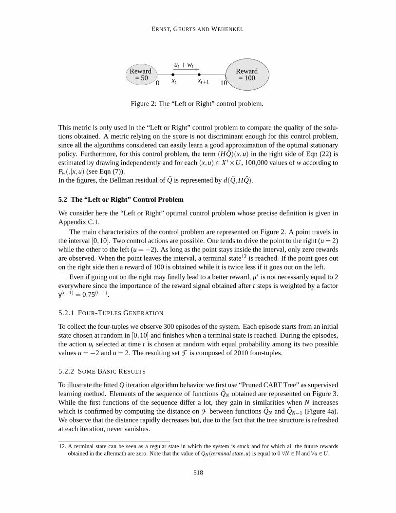
xt
ut +wtRewardReward
xt+1= 100= 50
0 10
Figure 2: The “Left or Right” control problem.
This metric is only used in the “Left or Right” control problem to compare the quality of the solu-tions obtained. A metric relying on the score is not discriminant enough for thiscontrol problem,since all the algorithms considered can easily learn a good approximation of the optimal stationarypolicy. Furthermore, for this control problem, the term(HQ)(x,u) in the right side of Eqn (22) isestimated by drawing independently and for each(x,u) ∈ Xi×U , 100,000 values ofw according toPw(.|x,u) (see Eqn (7)).In the figures, the Bellman residual ofQ is represented byd(Q,HQ).
5.2 The “Left or Right” Control Problem
We consider here the “Left or Right” optimal control problem whose precise definition is given inAppendix C.1.
The main characteristics of the control problem are represented on Figure 2. A point travels inthe interval[0,10]. Two control actions are possible. One tends to drive the point to the right(u= 2)while the other to the left (u =−2). As long as the point stays inside the interval, only zero rewardsare observed. When the point leaves the interval, a terminal state12 is reached. If the point goes outon the right side then a reward of 100 is obtained while it is twice less if it goes out on the left.
Even if going out on the right may finally lead to a better reward,µ∗ is not necessarily equal to 2everywhere since the importance of the reward signal obtained aftert steps is weighted by a factorγ(t−1) = 0.75(t−1).
5.2.1 FOUR-TUPLESGENERATION
To collect the four-tuples we observe 300 episodes of the system. Each episode starts from an initialstate chosen at random in[0,10] and finishes when a terminal state is reached. During the episodes,the actionut selected at timet is chosen at random with equal probability among its two possiblevaluesu =−2 andu = 2. The resulting setF is composed of 2010 four-tuples.
5.2.2 SOME BASIC RESULTS
To illustrate the fittedQ iteration algorithm behavior we first use “Pruned CART Tree” as supervisedlearning method. Elements of the sequence of functionsQN obtained are represented on Figure 3.While the first functions of the sequence differ a lot, they gain in similarities when N increaseswhich is confirmed by computing the distance onF between functionsQN andQN−1 (Figure 4a).We observe that the distance rapidly decreases but, due to the fact that the tree structure is refreshedat each iteration, never vanishes.
12. A terminal state can be seen as a regular state in which the system is stuckand for which all the future rewardsobtained in the aftermath are zero. Note that the value ofQN(terminal state,u) is equal to 0∀N ∈ N and∀u∈U .
518
TREE-BASED BATCH MODE REINFORCEMENTLEARNING
100.
75.
50.
25.
0.0
0.0 2.5 7.55. 10. x
Q1(x,−2)
Q1(x,2)
Q1100.
75.
50.
25.
0.0
0.0 2.5 7.55. 10. x
Q2
Q2(x,−2)
Q2(x,2)
0.0 2.5 7.55. 10. x
Q3
Q3(x,−2)
Q3(x,2)
100.
75.
50.
25.
0.0
0.0 2.5 7.55. 10. x
100.
75.
50.
25.
0.0
Q4(x,−2)
Q4(x,2)
Q4
0.0 2.5 7.55. 10. x
100.
75.
50.
25.
0.0
Q5
Q5(x,2)
Q5(x,−2)
0.0 2.5 7.55. 10. x
100.
75.
50.
25.
0.0
Q10
Q10(x,−2)
Q10(x,2)
Figure 3: Representation ofQN for different values ofN. The setF is composed of 2010 elements and thesupervised learning method used is Pruned CART Tree.
2 3 4 6 7 8 9 105
35.
30.
25.
20.
15.
10.
5.
0.0
N
d(QN,
QN−1)
1 2 3 4 5 6 7 8 9 10N
58.
60.
62.
64.
Jµ∗N∞
1 2 3 4 5 6 7 8 9 100.0
2.5
5.
7.5
10.
12.5
N
d(QN,
HQN)
(a) d(QN,QN−1) =∑#F
l=1(QN(xlt ,u
lt )−QN−1(x
lt ,u
lt ))
2
#F
(b) Jµ∗N∞ =
∑Xi Jµ∗N∞ (x)
#Xi
(c) d(QN,HQN) =∑Xi×U (QN(x,u)−(HQN)(x,u))2
#(Xi×U)
Figure 4: Figure (a) represents the distance betweenQN andQN−1. Figure (b) provides the average returnobtained by the policy ˆµ∗N while starting from an element ofXi . Figure (c) represents the Bellmanresidual ofQN.
519

ERNST, GEURTS AND WEHENKEL
From the functionQN we can determine the policy ˆµN. Statesx for whichQN(x,2)≥ QN(x,−2)correspond to a value of ˆµN(x) = 2 while µN(x) = −2 if QN(x,2) < QN(x,−2). For example, ˆµ∗10consists of choosingu = −2 on the interval[0,2.7[ andu = 2 on [2.7,10]. To associate a score toeach policyµ∗N, we define a set of statesXi = {0,1,2, · · · ,10}, evaluateJµN
∞ (x) for each element ofthis set and average the values obtained. The evolution of the score of ˆµ∗N with N is drawn on Figure4b. We observe that the score first increases rapidly to become finally almost constant for values ofN greater than 5.
In order to assess the quality of the functionsQN computed, we have computed the Bellmanresidual of theseQN-functions. We observe in Figure 4c that even if the Bellman residual tendstodecrease whenN increases, it does not vanish even for large values ofN. By observing Table 2, onecan however see that by using 6251 four-tuples (1000 episodes) rather than 2010 (300 episodes),the Bellman residual further decreases.
5.2.3 INFLUENCE OF THETREE-BASED METHOD
When dealing with such a system for which the dynamics is highly stochastic, pruning is necessary,even for tree-based methods producing an ensemble of regression trees. Figure 5 thus represents theQN-functions for different values ofN with the pruned version of the Extra-Trees. By comparingthis figure with Figure 3, we observe that the averaging of several treesproduces smoother functionsthan single regression trees.
By way of illustration, we have also used the Extra-Trees algorithm with fully developed trees(i.e.,nmin = 2) and computed theQ10-function with the fittedQ iteration using the same set of four-tuples as in the previous section. This function is represented in Figure 6. As fully grown trees areable to match perfectly the output in the training set, they also catch the noise andthis explains thechaotic nature of the resulting approximation.
Table 2 gathers the Bellman residuals ofQ10 obtained when using different tree-based methodsand this for different sets of four-tuples. Tree-based ensemble methods produce smaller Bellmanresiduals and among these methods, Extra-Trees behaves the best. We can also observe that for anyof the tree-based methods used, the Bellman residual decreases with the size of F .
Note that here, the policies produced by the different tree-based algorithms offer quite similarscores. For example, the score is 64.30 when Pruned CART Tree is applied to the 2010 four-tupleset and it does not differ from more than one percent with any of the other methods. We will seethat the main reason behind this, is the simplicity of the optimal control problem considered and thesmall dimensionality of the state space.
5.2.4 FITTED Q ITERATION AND BASIS FUNCTION METHODS
We now assess performances of the fittedQ iteration algorithm when combined with basis functionmethods. Basis function methods suppose a relation of the type
o =nbBasis
∑j=1
c jφ j(i) (23)
between the input and the output wherec j ∈ R and where the basis functionsφ j(i) are defined onthe input space and take their values onR. These basis functions form the approximation architec-
520
TREE-BASED BATCH MODE REINFORCEMENTLEARNING
100.
75.
50.
25.
0.0
0.0 2.5 7.55. 10. x
Q1
Q1(x,−2)
Q1(x,2)
100.
75.
50.
25.
0.0
0.0 2.5 7.55. 10. x
Q2
Q2(x,2)
Q2(x,−2)
0.0 2.5 7.55. 10. x
Q3100.
75.
50.
25.
0.0
Q3(x,−2)
Q3(x,2)
0.0 2.5 7.55. 10. x
100.
75.
50.
25.
0.0
Q4
Q4(x,2)
Q4(x,−2)
0.0 2.5 7.55. 10. x
100.
75.
50.
25.
0.0
Q5
Q5(x,−2)
Q5(x,2)
0.0 2.5 7.55. 10. x
100.
75.
50.
25.
0.0
Q10
Q10(x,−2)
Q10(x,2)
Figure 5: Representation ofQN for different values ofN. The setF is composed of 2010 elements and thesupervised learning method used is the Pruned Extra-Trees.
0.0 2.5 7.55. 10. x
100.
75.
50.
25.
0.0
Q10
Q10(x,−2)
Q10(x,2)
Figure 6: Representation ofQ10 when Extra-Trees is used with no pruning
Tree-basedmethod
#F
720 2010 6251Pruned CART Tree 2.62 1.96 1.29
Pruned Kd-Tree 1.94 1.31 0.76Pruned Tree Bagging 1.61 0.79 0.67Pruned Extra-Trees 1.29 0.60 0.49
Pruned Tot. Rand. Trees1.55 0.72 0.59
Table 2: Bellman residual ofQ10. Three differentsets of four-tuples are used. These setshave been generated by considering 100,300 and 1000 episodes and are composedrespectively of 720, 2010 and 6251 four-tuples.
ture. The training set is used to determine the values of the differentc j by solving the followingminimization problem:13
13. This minimization problem can be solved by building the(#T S× nbBasis) Y matrix with Yl j = φ j (i l ). If YTYis invertible, then the minimization problem has a unique solutionc = (c1,c2, · · · ,cnbBasis) given by the followingexpression:c = (YTY)−1YTb with b∈ R
#T S such thatbl = ol . In order to overcome the possible problem of non-invertibility of YTY that occurs when solution of (24) is not unique, we have added toYTY the strictly definite positivematrixδI , whereδ is a small positive constant, before inverting it. The value ofc used in our experiments as solutionof (24) is therefore equal to(YTY +δI)−1YTb whereδ has been chosen equal to 0.001.
521
ERNST, GEURTS AND WEHENKEL
Extra-Trees0.0
0.5
1.
1.5
2.
2.5
Gridsize
d(Q10,
HQ10)
10 20 30 40
piecewise-linear grid
piecewise-constant grid
0.0 2.5 5. 7.5 10.
0.0
25.
50.
75.
100.
Q10
x
Q10(x,2)
Q10(x,−2)
0.0 2.5 5. 7.5 10.
0.0
25.
50.
75.
100.
Q10
x
Q10(x,2)
Q10(x,−2)
(a) Bellman residual ofQ10
(b) Q10 computedwhen using a 28
piecewise-constantgrid as approx. arch.
(c) Q10 computed whenusing a 7 piecewise-linear
grid as approx. arch.
Figure 7: FittedQ iteration with basis function methods. Two different typesof approximation architecturesare considered: piecewise-constant and piecewise-lineargrids. 300 episodes are used to generateF .
argmin(c1,c2,··· ,cnbBasis)∈RnbBasis
#T S
∑l=1
(nbBasis
∑j=1
c jφ j(il )−ol )2
. (24)
We consider two different sets of basis functionsφ j . The first set is defined by partitioning thestate space into a grid and by considering one basis function for each gridcell, equal to the indicatorfunction of this cell. This leads to piecewise constantQ-functions. The other type is defined bypartitioning the state space into a grid, triangulating every element of the grid and considering thatQ(x,u) = ∑v∈Vertices(x)W(x,v)Q(v,u) whereVertices(x) is the set of vertices of the hypertrianglexbelongs to andW(x,v) is the barycentric coordinate ofx that corresponds tov. This leads to a set ofoverlapping piecewise linear basis functions, and yields a piecewise linearand continuous model.In this paper, these approximation architectures are respectively referred to aspiecewise-constantgrid andpiecewise-linear grid. The reader can refer to Ernst (2003) for more information.
To assess performances of fittedQ iteration combined with piecewise-constant and piecewise-linear grids as approximation architectures, we have used several grid resolutions to partition theinterval [0,10] (a 5 grid, a 6 grid,· · · , a 50 grid). For each grid, we have used fittedQ iterationwith each of the two types of approximation architectures and computedQ10. The Bellman resid-uals obtained by the differentQ10-functions are represented on Figure 7a. We can see that basisfunction methods with piecewise-constant grids perform systematically worse than Extra-Trees, thetree-based method that produces the lowest Bellman residual. This type of approximation archi-tecture leads to the lowest Bellman residual for a 28 grid and the corresponding Q10-function issketched in Figure 7b. Basis function methods with piecewise-linear grids reach their lowest Bell-man residual for a 7 grid, Bellman residual that is smaller than the one obtainedby Extra-Trees.The corresponding smootherQ10-function is drawn on Figure 7b.
Even if piecewise-linear grids were able to produce on this example better results than the tree-based methods, it should however be noted that it has been achieved by tuning the grid resolutionand that this resolution strongly influences the quality of the solution. We will see below that, as the
522

TREE-BASED BATCH MODE REINFORCEMENTLEARNING
state space dimensionality increases, piecewise-constant or piecewise-linear grids do not competeanymore with tree-based methods. Furthermore, we will also observe that piecewise-linear gridsmay lead to divergence to infinity of the fittedQ iteration algorithm (see Section 5.3.3).
5.3 The “Car on the Hill” Control Problem
We consider here the “Car on the Hill” optimal control problem whose precise definition is given inAppendix C.2.
A car modeled by a point mass is traveling on a hill (the shape of which is givenby the func-tion Hill (p) of Figure 8b). The actionu acts directly on the acceleration of the car (Eqn (31),Appendix C) and can only assume two extreme values (full acceleration (u = 4) or full deceleration(u =−4)). The control problem objective is roughly to bring the car in a minimum time to the topof the hill (p = 1 in Figure 8b) while preventing the positionp of the car to become smaller than−1 and its speeds to go outside the interval[−3,3]. This problem has a (continuous) state space ofdimension two (the positionp and the speeds of the car) represented on Figure 8a.
Note that by exploiting the particular structure of the system dynamics and the reward functionof this optimal control problem, it is possible to determine with a reasonable amount of computationthe exact value ofJµ∗
∞ (Q) for any statex (state-action pair(x,u)).14
3.
2.
1.
0.0
−1.
−2.
−3.
−1. −.5 0.0 0.5 1.
s
p
p
u
−0.2
0.2
0.4
−1. −.5 0.0 0.5 1.
Resistance
mg
Hill (p)
(a)X \{terminal state} (b)Representation ofHill (p) (shape of the hill) and
of the different forces applied to the car.
Figure 8: The “Car on the Hill” control problem.
5.3.1 SOME BASIC RESULTS
To generate the four-tuples we consider episodes starting from the same initial state correspondingto the car stopped at the bottom of the hill (i.e.,(p,s) = (−0.5,0) ) and stopping when the car leavesthe region represented on Figure 8a (i.e., when a terminal state is reached). In each episode, theactionut at each time step is chosen with equal probability among its two possible valuesu = −4andu= 4. We consider 1000 episodes. The corresponding setF is composed of 58090 four-tuples.Note that during these 1000 episodes the rewardr(xt ,ut ,wt) = 1 (corresponding to an arrival of thecar at the top of the hill with a speed comprised in[−3,3]) has been observed only 18 times.
14. To computeJµ∗∞ (x), we determine by successive trials the smallest value ofk for which one of the two following
conditions is satisfied (i) at least one sequence of actions of lengthk leads to a reward equal to 1 whenx0 = x (ii) all
523
ERNST, GEURTS AND WEHENKEL
3.
2.
1.
0.0
−1.
−2.
−3.
−1. −.5 0.0 0.5 1.
s
p
3.
2.
1.
0.0
−1.
−2.
−3.
−1. −.5 0.0 0.5 1.
s
p
3.
2.
1.
0.0
−1.
−2.
−3.
−1. −.5 0.0 0.5 1.
s
p
(a) argmaxu∈U
Q1(x,u) (b) argmaxu∈U
Q5(x,u) (c) argmaxu∈U
Q10(x,u)
3.
2.
1.
0.0
−1.
−2.
−3.
−1. −.5 0.0 0.5 1.
s
p
3.
2.
1.
0.0
−1.
−2.
−3.
−1. −.5 0.0 0.5 1.
s
p
3.
2.
1.
0.0
−1.
−2.
−3.
−1. −.5 0.0 0.5 1.
s
p
(d) argmaxu∈U
Q20(x,u) (e) argmaxu∈U
Q50(x,u) (f) Trajectory
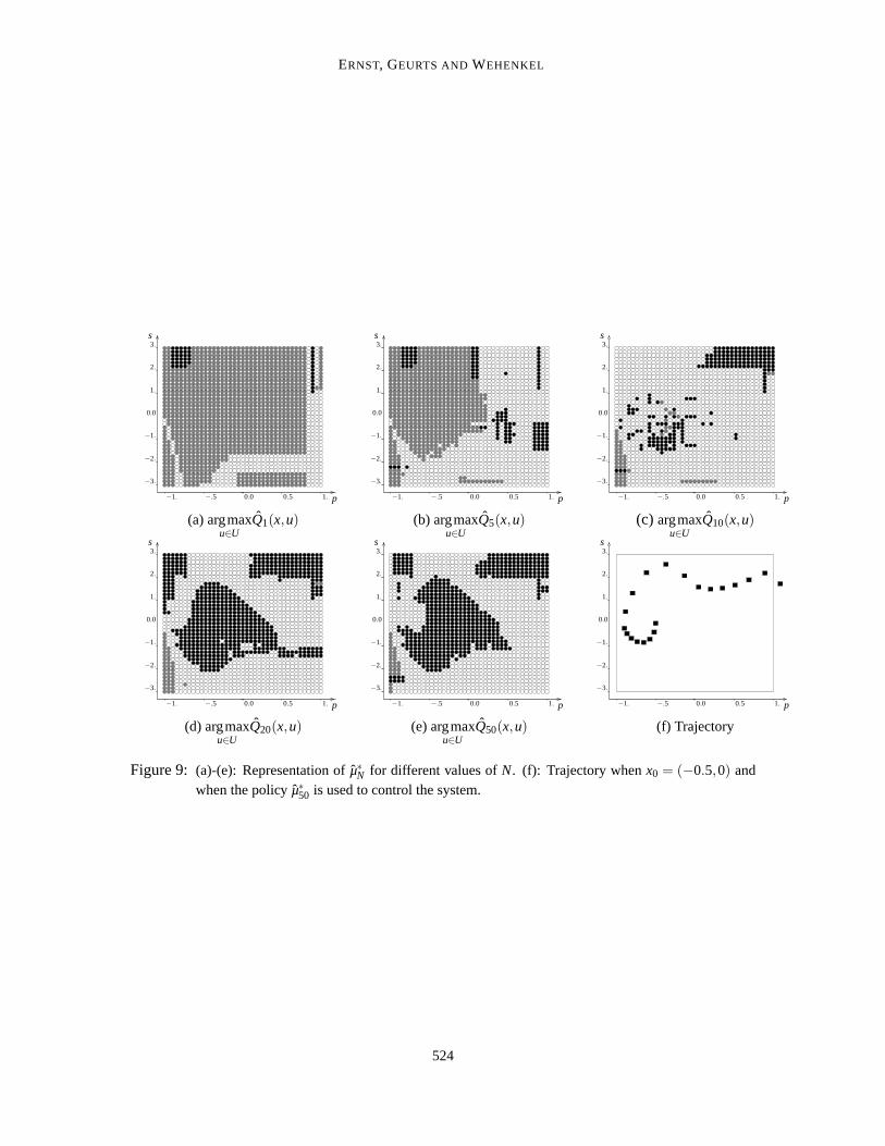
Figure 9: (a)-(e): Representation of ˆµ∗N for different values ofN. (f): Trajectory whenx0 = (−0.5,0) andwhen the policy ˆµ∗50 is used to control the system.
524
TREE-BASED BATCH MODE REINFORCEMENTLEARNING
N
QN−1)d(QN,
10 20 30 40 500.0
0.001
0.002
0.003
0.004
0.005
0.006
N
Jµ∗N∞
0.0
0.1
0.2
0.3
−0.1
−0.2
−0.3
−0.4
10 20 30 40 50
0.25
0.2
0.15
0.1
0.05
0.010 20 30 40 50N
d(QN,Q)
d(QN,HQN)
d(QN, .)
(a) d(QN,QN−1) =∑#F
l=1(QN(xlt ,u
lt )−QN−1(x
lt ,u
lt ))
2
#F
(b) Jµ∗N∞ =
∑Xi Jµ∗N∞ (x)
#Xi
(c) d(QN,F) =∑Xi×U (QN(x,u)−F(x,u))2
#(Xi×U)
F = QorHQN
Figure 10: Figure (a) represents the distance betweenQN andQN−1. Figure (b) provides the average returnobtained by the policy ˆµ∗N while starting from an element ofXi . Figure (c) represents the distancebetweenQN andQ as well as the Bellman residual ofQN as a function ofN (distance betweenQN andHQN).
We first use Tree Bagging as the supervised learning method. As the actionspace is binary, weagain model the functionsQN(x,−4) andQN(x,4) by two ensembles of 50 trees each, andnmin = 2.The policy µ∗1 so obtained is represented on Figure 9a. Black bullets represent states for whichQ1(x,−4) > Q1(x,4), white bullets states for whichQ1(x,−4) < Q1(x,4) and grey bullets states forwhich Q1(x,−4) = Q1(x,4). Successive policies ˆµ∗N for increasingN are given on Figures 9b-9e.
On Figure 9f, we have represented the trajectory obtained when starting from (s, p) = (−0.5,0)and using the policy ˆµ∗50 to control the system. Since, for this particular state the computation ofJµ∗
∞
gives the same value asJµ∗50∞ , the trajectory drawn is actually an optimal one.
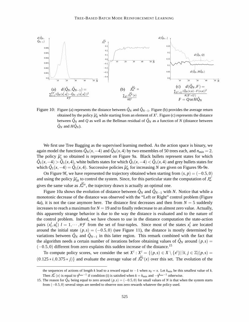
Figure 10a shows the evolution of distance betweenQN andQN−1 with N. Notice that while amonotonic decrease of the distance was observed with the “Left or Right” control problem (Figure4a), it is not the case anymore here. The distance first decreases andthen fromN = 5 suddenlyincreases to reach a maximum forN = 19 and to finally redecrease to an almost zero value. Actually,this apparently strange behavior is due to the way the distance is evaluated and to the nature ofthe control problem. Indeed, we have chosen to use in the distance computation the state-actionpairs (xl
t ,ult) l = 1, · · · ,#F from the set of four-tuples. Since most of the statesxl
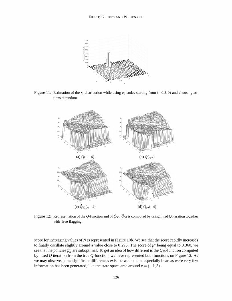
t are locatedaround the initial state(p,s) = (−0.5,0) (see Figure 11), the distance is mostly determined byvariations betweenQN and QN−1 in this latter region. This remark combined with the fact thatthe algorithm needs a certain number of iterations before obtaining values ofQN around(p,s) =(−0.5,0) different from zero explains this sudden increase of the distance.15
To compute policy scores, we consider the setXi : Xi = {(p,s) ∈ X \ {xt}|∃i, j ∈ Z|(p,s) =
(0.125∗ i,0.375∗ j)} and evaluate the average value ofJµ∗N∞ (x) over this set. The evolution of the
the sequences of actions of lengthk lead to a reward equal to−1 whenx0 = x. Let kmin be this smallest value ofk.ThenJµ∗
∞ (x) is equal toγkmin−1 if condition (i) is satisfied whenk = kmin and−γkmin−1 otherwise.15. The reason forQN being equal to zero around(p,s) = (−0.5,0) for small values ofN is that when the system starts
from (−0.5,0) several steps are needed to observe non zero rewards whatever thepolicy used.
525
ERNST, GEURTS AND WEHENKEL
−1−0.5
00.5
1
−3
−2
−1
0
1
2
30
0.005
0.01
0.015
0.02
0.025
0.03
0.035
0.04
ps
Fre
quen
cy o
f vis
it of
a ti
le
Figure 11: Estimation of thext distribution while using episodes starting from(−0.5,0) and choosing ac-tions at random.
−1
−0.5
0
0.5
1
−3
−2
−1
0
1
2
3
−1
−0.5
0
0.5
1
−1
−0.5
0
0.5
1
−3
−2
−1
0
1
2
3
−1
−0.5
0
0.5
1
(a)Q(.,−4) (b) Q(.,4)
−1
−0.5
0
0.5
1
−3
−2
−1
0
1
2
3
−1
−0.5
0
0.5
1
−1
−0.5
0
0.5
1
−3
−2
−1
0
1
2
3
−1
−0.5
0
0.5
1
(c) Q50(.,−4) (d) Q50(.,4)
Figure 12: Representation of theQ-function and ofQ50. Q50 is computed by using fittedQ iteration togetherwith Tree Bagging.
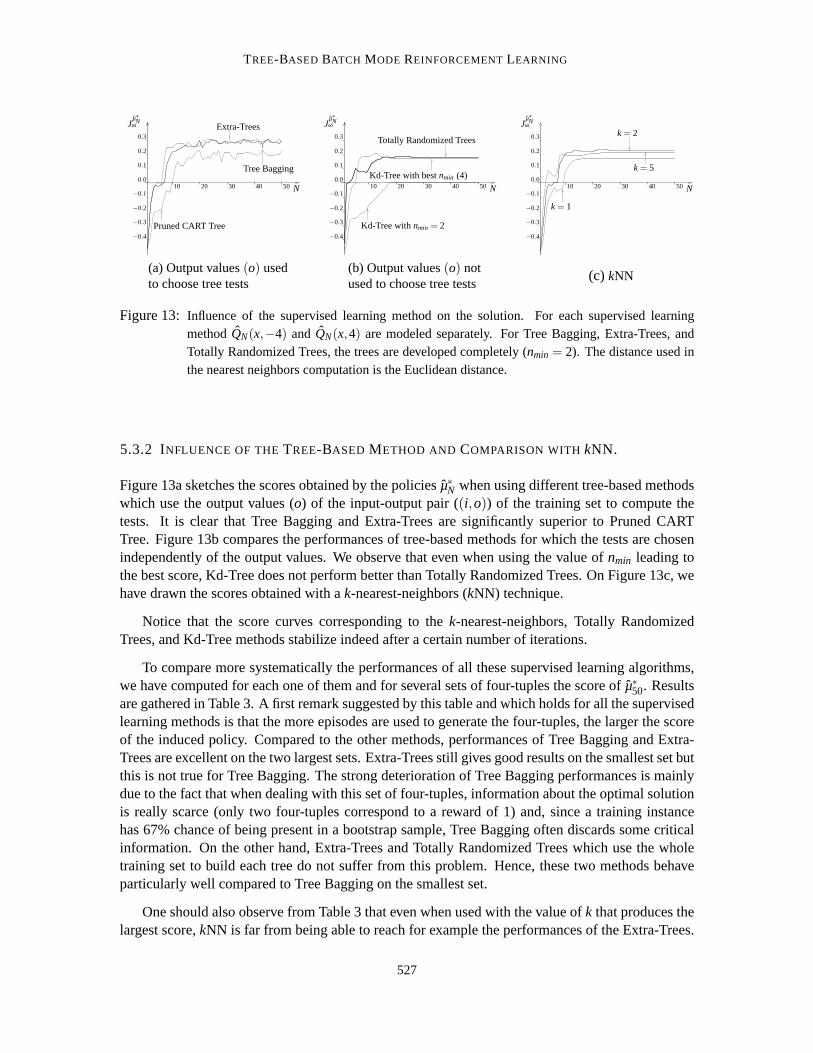
score for increasing values ofN is represented in Figure 10b. We see that the score rapidly increasesto finally oscillate slightly around a value close to 0.295. The score ofµ∗ being equal to 0.360, wesee that the policies ˆµ∗N are suboptimal. To get an idea of how different is theQ50-function computedby fittedQ iteration from the trueQ-function, we have represented both functions on Figure 12. Aswe may observe, some significant differences exist between them, especially in areas were very fewinformation has been generated, like the state space area aroundx = (−1,3).
526
TREE-BASED BATCH MODE REINFORCEMENTLEARNING
N
0.3
0.2
0.1
0.010 20 30 40 50
Jµ∗N∞
Tree Bagging
Pruned CART Tree
Extra-Trees
−0.1
−0.2
−0.3
−0.4
N
0.3
0.2
0.1
0.010 20 30 40 50
Jµ∗N∞
Kd-Tree with bestnmin (4)
Kd-Tree withnmin = 2
Totally Randomized Trees
−0.1
−0.2
−0.3
−0.4
N
0.3
0.2
0.1
0.010 20 30 40 50
Jµ∗N∞
k = 2
k = 5
k = 1
−0.1
−0.2
−0.3
−0.4
(a) Output values(o) usedto choose tree tests
(b) Output values(o) notused to choose tree tests
(c) kNN
Figure 13: Influence of the supervised learning method on the solution.For each supervised learningmethodQN(x,−4) and QN(x,4) are modeled separately. For Tree Bagging, Extra-Trees, andTotally Randomized Trees, the trees are developed completely (nmin = 2). The distance used inthe nearest neighbors computation is the Euclidean distance.
5.3.2 INFLUENCE OF THETREE-BASED METHOD AND COMPARISON WITH kNN.
Figure 13a sketches the scores obtained by the policies ˆµ∗N when using different tree-based methodswhich use the output values (o) of the input-output pair ((i,o)) of the training set to compute thetests. It is clear that Tree Bagging and Extra-Trees are significantly superior to Pruned CARTTree. Figure 13b compares the performances of tree-based methods for which the tests are chosenindependently of the output values. We observe that even when using thevalue ofnmin leading tothe best score, Kd-Tree does not perform better than Totally Randomized Trees. On Figure 13c, wehave drawn the scores obtained with ak-nearest-neighbors (kNN) technique.
Notice that the score curves corresponding to thek-nearest-neighbors, Totally RandomizedTrees, and Kd-Tree methods stabilize indeed after a certain number of iterations.
To compare more systematically the performances of all these supervised learning algorithms,we have computed for each one of them and for several sets of four-tuples the score of ˆµ∗50. Resultsare gathered in Table 3. A first remark suggested by this table and which holds for all the supervisedlearning methods is that the more episodes are used to generate the four-tuples, the larger the scoreof the induced policy. Compared to the other methods, performances of Tree Bagging and Extra-Trees are excellent on the two largest sets. Extra-Trees still gives good results on the smallest set butthis is not true for Tree Bagging. The strong deterioration of Tree Bagging performances is mainlydue to the fact that when dealing with this set of four-tuples, information about the optimal solutionis really scarce (only two four-tuples correspond to a reward of 1) and, since a training instancehas 67% chance of being present in a bootstrap sample, Tree Bagging often discards some criticalinformation. On the other hand, Extra-Trees and Totally Randomized Treeswhich use the wholetraining set to build each tree do not suffer from this problem. Hence, these two methods behaveparticularly well compared to Tree Bagging on the smallest set.
One should also observe from Table 3 that even when used with the value of k that produces thelargest score,kNN is far from being able to reach for example the performances of the Extra-Trees.
527
ERNST, GEURTS AND WEHENKEL
Supervised learningmethod
Nb of episodes usedto generateF
1000 300 100Kd-Tree (Bestnmin) 0.17 0.16 -0.06Pruned CART Tree 0.23 0.13 -0.26
Tree Bagging 0.30 0.24 -0.09Extra-Trees 0.29 0.25 0.12
Totally Randomized Trees 0.18 0.14 0.11kNN (Bestk) 0.23 0.18 0.02
Table 3:Score ofµ∗50 for different set of four-tuples and supervised learning methods.
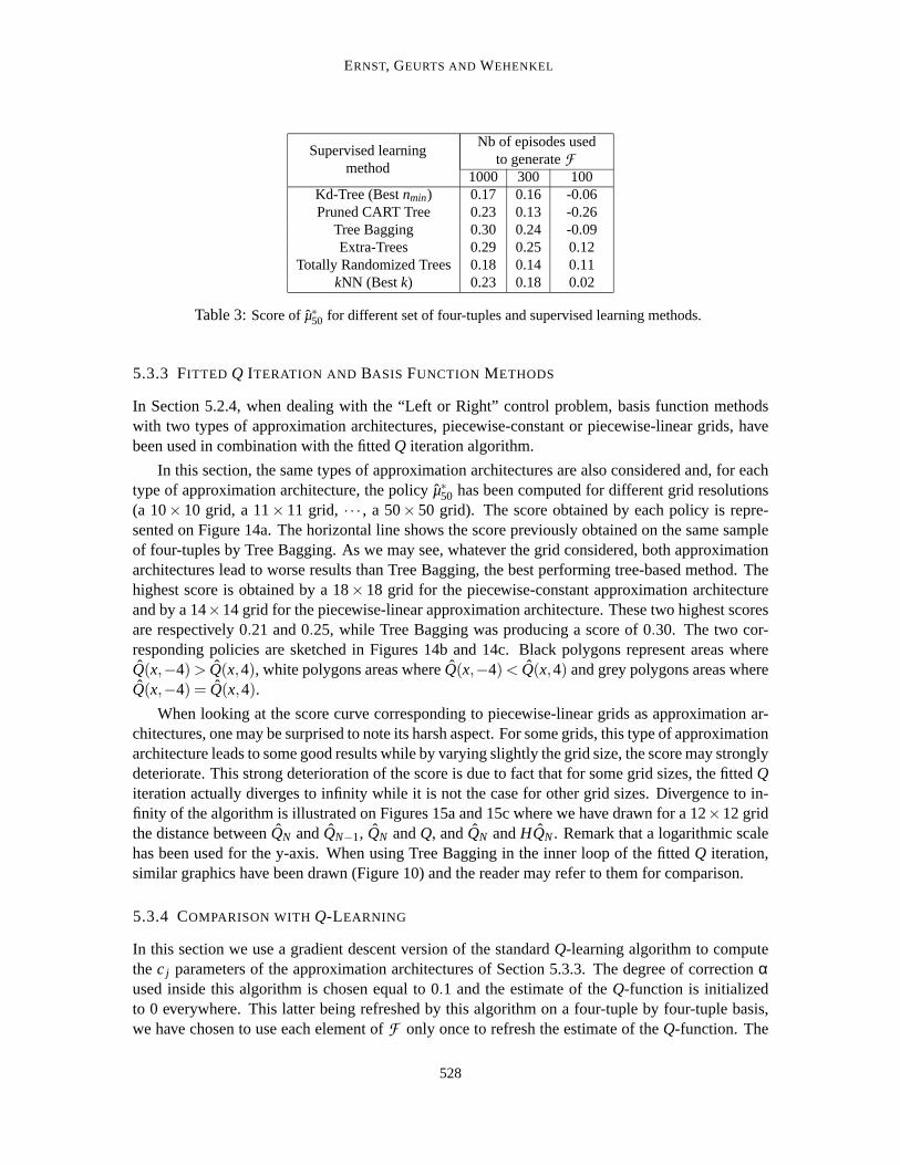
5.3.3 FITTED Q ITERATION AND BASIS FUNCTION METHODS
In Section 5.2.4, when dealing with the “Left or Right” control problem, basisfunction methodswith two types of approximation architectures, piecewise-constant or piecewise-linear grids, havebeen used in combination with the fittedQ iteration algorithm.
In this section, the same types of approximation architectures are also considered and, for eachtype of approximation architecture, the policy ˆµ∗50 has been computed for different grid resolutions(a 10×10 grid, a 11×11 grid, · · · , a 50×50 grid). The score obtained by each policy is repre-sented on Figure 14a. The horizontal line shows the score previously obtained on the same sampleof four-tuples by Tree Bagging. As we may see, whatever the grid considered, both approximationarchitectures lead to worse results than Tree Bagging, the best performing tree-based method. Thehighest score is obtained by a 18×18 grid for the piecewise-constant approximation architectureand by a 14×14 grid for the piecewise-linear approximation architecture. These two highest scoresare respectively 0.21 and 0.25, while Tree Bagging was producing a score of 0.30. The two cor-responding policies are sketched in Figures 14b and 14c. Black polygons represent areas whereQ(x,−4) > Q(x,4), white polygons areas whereQ(x,−4) < Q(x,4) and grey polygons areas whereQ(x,−4) = Q(x,4).
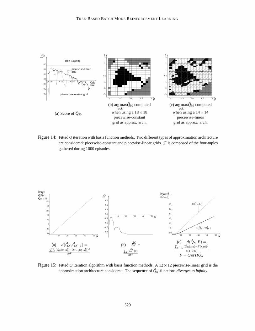
When looking at the score curve corresponding to piecewise-linear grids as approximation ar-chitectures, one may be surprised to note its harsh aspect. For some grids,this type of approximationarchitecture leads to some good results while by varying slightly the grid size, the score may stronglydeteriorate. This strong deterioration of the score is due to fact that for some grid sizes, the fittedQiteration actually diverges to infinity while it is not the case for other grid sizes. Divergence to in-finity of the algorithm is illustrated on Figures 15a and 15c where we have drawn for a 12×12 gridthe distance betweenQN andQN−1, QN andQ, andQN andHQN. Remark that a logarithmic scalehas been used for the y-axis. When using Tree Bagging in the inner loop of the fittedQ iteration,similar graphics have been drawn (Figure 10) and the reader may refer tothem for comparison.
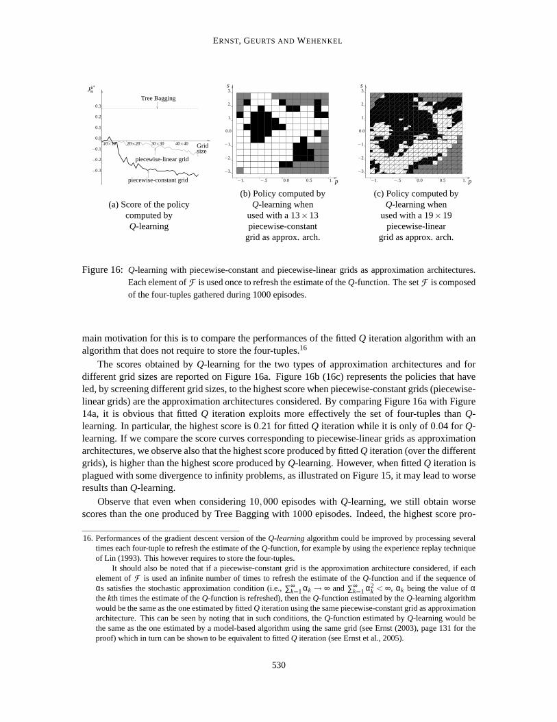
5.3.4 COMPARISON WITH Q-LEARNING
In this section we use a gradient descent version of the standardQ-learning algorithm to computethec j parameters of the approximation architectures of Section 5.3.3. The degreeof correctionαused inside this algorithm is chosen equal to 0.1 and the estimate of theQ-function is initializedto 0 everywhere. This latter being refreshed by this algorithm on a four-tuple by four-tuple basis,we have chosen to use each element ofF only once to refresh the estimate of theQ-function. The
528
TREE-BASED BATCH MODE REINFORCEMENTLEARNING
Gridsize
10×10 20×20 30×30 40×40
−0.3
−0.2
−0.1
0.0
0.1
0.2
0.3
Tree Bagging
Jµ∗50∞
gridpiecewise-linear
piecewise-constant grid
3.
2.
1.
0.0
−1.
−2.
−3.
−1. −.5 0.0 0.5 1.
s
p
3.
2.
1.
0.0
−1.
−2.
−3.
−1. −.5 0.0 0.5 1.
s
p
(a) Score ofQ50
(b) argmaxu∈U
Q50 computed
when using a 18×18piecewise-constant
grid as approx. arch.
(c) argmaxu∈U
Q50 computed
when using a 14×14piecewise-linear
grid as approx. arch.
Figure 14: FittedQ iteration with basis function methods. Two different typesof approximation architectureare considered: piecewise-constant and piecewise-lineargrids.F is composed of the four-tuplesgathered during 1000 episodes.
10 20 30 40 500.0
2.5
5.
7.5
10.
12.5
15.
17.5
N
log10(d(QN,
QN−1))
N
Jµ∗N∞
0.0
0.1
0.2
0.3
−0.1
−0.2
−0.3
−0.4
10 20 30 40 50
10 20 30 40 500.0
5.
10.
15.
20.
25.
30.
log10(d(QN, .))
N
d(QN,Q)
d(QN,HQN)
(a) d(QN,QN−1) =∑#F
l=1(QN(xlt ,u
lt )−QN−1(x
lt ,u
lt ))
2
#F
(b) Jµ∗N∞ =
∑Xi Jµ∗N∞ (x)
#Xi
(c) d(QN,F) =∑Xi×U (QN(x,u)−F(x,u))2
#(Xi×U)
F = QorHQN
Figure 15: FittedQ iteration algorithm with basis function methods. A 12×12 piecewise-linear grid is theapproximation architecture considered. The sequence ofQN-functionsdiverges to infinity.
529
ERNST, GEURTS AND WEHENKEL
Gridsize
10×10 20×20 30×30 40×40
−0.3
−0.2
−0.1
0.0
0.1
0.2
0.3
Tree Bagging
Jµ∗∞
piecewise-constant grid
piecewise-linear grid
3.
2.
1.
0.0
−1.
−2.
−3.
−1. −.5 0.0 0.5 1.
s
p
3.
2.
1.
0.0
−1.
−2.
−3.
−1. −.5 0.0 0.5 1.
s
p
(a) Score of the policycomputed byQ-learning
(b) Policy computed byQ-learning when
used with a 13×13piecewise-constant
grid as approx. arch.
(c) Policy computed byQ-learning when
used with a 19×19piecewise-linear
grid as approx. arch.
Figure 16: Q-learning with piecewise-constant and piecewise-linear grids as approximation architectures.Each element ofF is used once to refresh the estimate of theQ-function. The setF is composedof the four-tuples gathered during 1000 episodes.
main motivation for this is to compare the performances of the fittedQ iteration algorithm with analgorithm that does not require to store the four-tuples.16
The scores obtained byQ-learning for the two types of approximation architectures and fordifferent grid sizes are reported on Figure 16a. Figure 16b (16c) represents the policies that haveled, by screening different grid sizes, to the highest score when piecewise-constant grids (piecewise-linear grids) are the approximation architectures considered. By comparing Figure 16a with Figure14a, it is obvious that fittedQ iteration exploits more effectively the set of four-tuples thanQ-learning. In particular, the highest score is 0.21 for fittedQ iteration while it is only of 0.04 for Q-learning. If we compare the score curves corresponding to piecewise-linear grids as approximationarchitectures, we observe also that the highest score produced by fitted Q iteration (over the differentgrids), is higher than the highest score produced byQ-learning. However, when fittedQ iteration isplagued with some divergence to infinity problems, as illustrated on Figure 15,it may lead to worseresults thanQ-learning.
Observe that even when considering 10,000 episodes withQ-learning, we still obtain worsescores than the one produced by Tree Bagging with 1000 episodes. Indeed, the highest score pro-
16. Performances of the gradient descent version of theQ-learningalgorithm could be improved by processing severaltimes each four-tuple to refresh the estimate of theQ-function, for example by using the experience replay techniqueof Lin (1993). This however requires to store the four-tuples.
It should also be noted that if a piecewise-constant grid is the approximation architecture considered, if eachelement ofF is used an infinite number of times to refresh the estimate of theQ-function and if the sequence ofαs satisfies the stochastic approximation condition (i.e.,∑∞
k=1 αk→ ∞ and∑∞k=1 α2
k < ∞, αk being the value ofαthekth times the estimate of theQ-function is refreshed), then theQ-function estimated by theQ-learning algorithmwould be the same as the one estimated by fittedQ iteration using the same piecewise-constant grid as approximationarchitecture. This can be seen by noting that in such conditions, theQ-function estimated byQ-learning would bethe same as the one estimated by a model-based algorithm using the same grid(see Ernst (2003), page 131 for theproof) which in turn can be shown to be equivalent to fittedQ iteration (see Ernst et al., 2005).
530
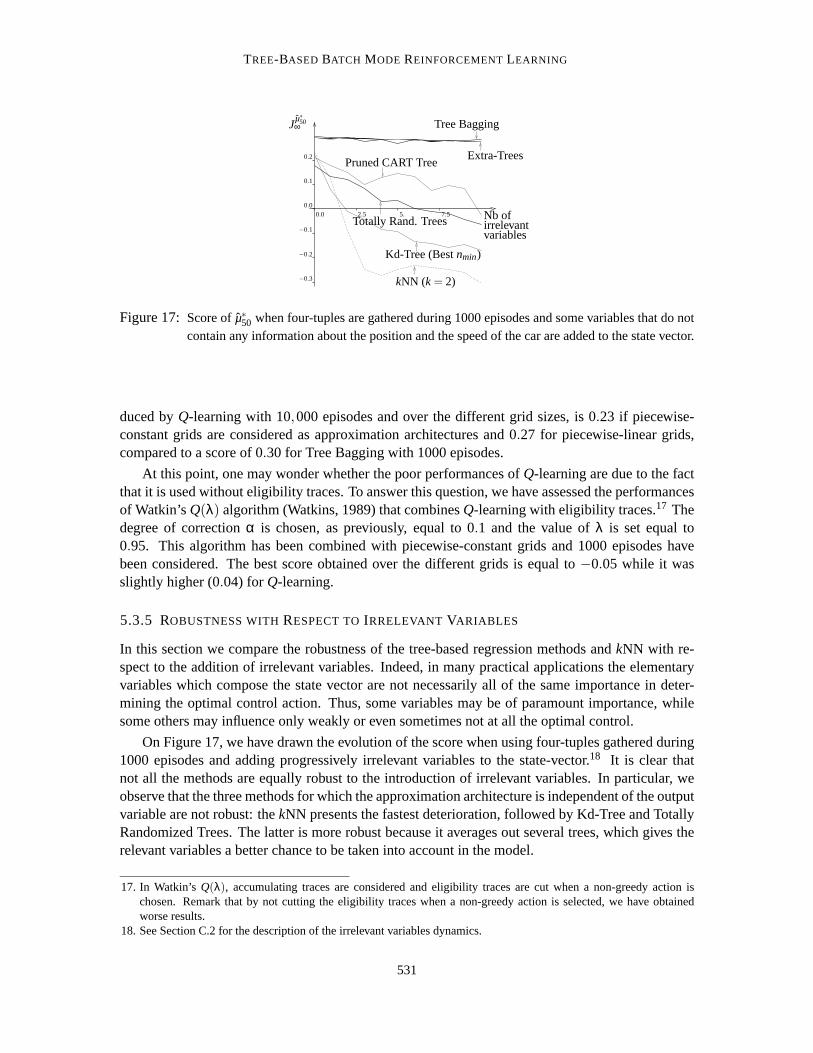
TREE-BASED BATCH MODE REINFORCEMENTLEARNING
0.2
0.1
0.00.0 2.5 5. 7.5
Jµ∗50∞
kNN (k = 2)
Kd-Tree (Bestnmin)
Pruned CART Tree
Tree Bagging
Extra-Trees
Totally Rand. Trees Nb ofirrelevantvariables
−0.1
−0.2
−0.3
Figure 17: Score ofµ∗50 when four-tuples are gathered during 1000 episodes and somevariables that do notcontain any information about the position and the speed of the car are added to the state vector.
duced byQ-learning with 10,000 episodes and over the different grid sizes, is 0.23 if piecewise-constant grids are considered as approximation architectures and 0.27 for piecewise-linear grids,compared to a score of 0.30 for Tree Bagging with 1000 episodes.
At this point, one may wonder whether the poor performances ofQ-learning are due to the factthat it is used without eligibility traces. To answer this question, we have assessed the performancesof Watkin’sQ(λ) algorithm (Watkins, 1989) that combinesQ-learning with eligibility traces.17 Thedegree of correctionα is chosen, as previously, equal to 0.1 and the value ofλ is set equal to0.95. This algorithm has been combined with piecewise-constant grids and 1000 episodes havebeen considered. The best score obtained over the different grids isequal to−0.05 while it wasslightly higher (0.04) forQ-learning.
5.3.5 ROBUSTNESS WITHRESPECT TOIRRELEVANT VARIABLES
In this section we compare the robustness of the tree-based regression methods andkNN with re-spect to the addition of irrelevant variables. Indeed, in many practical applications the elementaryvariables which compose the state vector are not necessarily all of the sameimportance in deter-mining the optimal control action. Thus, some variables may be of paramount importance, whilesome others may influence only weakly or even sometimes not at all the optimal control.
On Figure 17, we have drawn the evolution of the score when using four-tuples gathered during1000 episodes and adding progressively irrelevant variables to the state-vector.18 It is clear thatnot all the methods are equally robust to the introduction of irrelevant variables. In particular, weobserve that the three methods for which the approximation architecture is independent of the outputvariable are not robust: thekNN presents the fastest deterioration, followed by Kd-Tree and TotallyRandomized Trees. The latter is more robust because it averages out several trees, which gives therelevant variables a better chance to be taken into account in the model.
17. In Watkin’sQ(λ), accumulating traces are considered and eligibility traces are cut when a non-greedy action ischosen. Remark that by not cutting the eligibility traces when a non-greedyaction is selected, we have obtainedworse results.
18. See Section C.2 for the description of the irrelevant variables dynamics.
531

ERNST, GEURTS AND WEHENKEL
On the other hand, the methods which take into account the output variables intheir approxima-tion architecture are all significantly more robust than the former ones. Among them, Tree Baggingand Extra-Trees which are based on the averaging of several trees are almost totally immune, sinceeven with 10 irrelevant variables (leading to the a 12-dimensional input space) their score decreaseis almost insignificant.
This experiment shows that the regression tree based ensemble methods which adapt their kernelto the output variable may have a strong advantage in terms of robustness over methods with a kernelwhich is independent of the output, even if these latter have nicer convergence properties.
5.3.6 INFLUENCE OF THENUMBER OF REGRESSIONTREES IN AN ENSEMBLE
In this paper, we have chosen to build ensembles of regression trees composed of 50 trees (M = 50,Section 4.2), a number of elements which, according to our simulations, is largeenough to ensurethat accuracy of the models produced could not be improved significantly by increasing it. In orderto highlight the influence ofM on the quality of the solution obtained, we have drawn on Figure18, for the different regression tree based ensemble methods, the qualityof the solution obtainedas a function ofM. We observe that the score grows rapidly withM, especially with Extra-Treesand Tree Bagging in which cases a value ofM = 10 would have been sufficient to obtain a goodsolution.
Note that since the CPU times required to compute the solution grow linearly with the numberof trees built, computational requirements of the regression tree based ensemble methods could beadjusted by choosing a value ofM.
302010 40
0.25
0.2
0.15
0.1
0.05
0.0
−0.1
−0.05
Jµ∗50∞ Tree Bagging
built (M)Nb of trees
Totally Randomized Trees
Extra-Trees
Figure 18: Evolution of the score of ˆµ∗50 with the number of trees built.F is composed of the four-tuplesgathered during 300 episodes.
5.3.7 CAR ON THE HILL WITH CONTINUOUS ACTION SPACE
To illustrate the use of the fittedQ iteration algorithm with continuous action spaces we considerhereU = [−4,4] rather than{−4,4}. We use one-step episodes with(x0,u0) drawn at random withuniform probability inX×U to generate a setF of 50,000 four-tuples and use Tree Bagging with 50trees as supervised learning method. We have approximated the maximization over the continuousaction space needed during the training sample refreshment step (see Eqn(13), Figure 1) by anexhaustive search overu∈ {−4,−3, · · · ,3,4}. The policyµ∗50 thus obtained by our algorithm after
532

TREE-BASED BATCH MODE REINFORCEMENTLEARNING
3.
2.
1.
0.0
−1.
−2.
−3.
−1. −.5 0.0 0.5 1.
s
p
0.35
0.3
0.25
0.2
0.1
1 model built
Continuous action space
Discrete action space
2 models built (1 for each value of u)
0.15
Nb offour-tuples
10000 20000 30000 40000
Jµ∗50∞
(a) Representation of ˆµ∗50 (b) Influence of #F on the score of the policy ˆµ∗50
Figure 19: Car on the Hill with continuous action space. Tree Bagging isused on one-step episodes with(x0,u0) drawn at random inX×U are used to generate the four-tuples.
50 iterations is represented on Figure 19a, where black bullets are used torepresent statesx forwhich µ∗50(x) is negative, white ones when ˆµ∗50(x) is positive. The size of a bullet is proportional tothe absolute value of the control signal|µ∗50(x)|. We see that the control policy obtained is not farfrom a “bang-bang” policy.
To compare these results with those obtained in similar conditions with a discrete action space,we have made two additional experiments, where the action space is restrictedagain to the extremevalues, i.e.u∈ {−4,4}. The two variants differ in the way theQN-functions are modeled. Namely,in the first case one single model is learned whereu is included in the input variables whereas in thesecond case one model is learned per possible value ofu, i.e. one model forQN(x,−4) and one forQN(x,4). All experiments are carried out for an increasing number of samples anda fixed numberof iterations (N = 50) and bagged trees (M = 50). The three curves of Figure 19b show the resultingscores. The two upper curves correspond to the score of the policy ˆµ∗50 obtained when considering adiscrete action spaceU = {−4,4}. We observe that both curves are close to each other and dominatethe “Continuous action space” scores. Obviously the discrete approachis favored because of the“bang-bang” nature of the problem; nevertheless, the continuous actionspace approach is able toprovide results of comparable quality.19
5.3.8 COMPUTATIONAL COMPLEXITY AND CPU TIME CONSIDERATIONS
Table 4 gathers the CPU times required by the fittedQ iteration algorithm to carry out 50 iterations(i.e., to computeQ50(x,u)) for different types of supervised learning methods and different sets F .We have also given in the same table the repartition of the CPU times between the twotasks thealgorithm has to perform, namely the task which consists of building the training sets (evaluationof Eqns (12) and (13) for alll ∈ {1,2, · · · ,#F }) and the task which consists of building the modelsfrom the training sets. These two tasks are referred to hereafter respectively as the “Training Set
19. The bang-bang nature was also observed in Smart and Kaelbling (2000), where continuous and a discrete actionspaces are treated on the “Car on the Hill” problem, with qualitatively the sameresults.
533

ERNST, GEURTS AND WEHENKEL
Building” (TSB) task and the “Model Building” (MB) task. When Kd-Tree or Totally RandomizedTrees are used, each tree structure is frozen after the first iteration and only the value of its terminalnodes are refreshed. The supervised learning technique referredto in the table as “kNN smart” is asmart implementation the fittedQ iteration algorithm when used withkNN in the sense that theknearest neighbors ofxl
t+1 are determined only once and not recomputed at each subsequent iterationof the algorithm.
Supervisedlearning
algorithm
CPU times consumed by the Models Building (MB)and Training Sets Building (TSB) tasks
#F = 5000 #F = 10000 #F = 20000MB TSB Total MB TSB Total MB TSB Total
Kd-Tree (nmin=4) 0.01 0.39 0.40 0.04 0.91 0.95 0.06 2.05 2.11Pruned CART Tree16.6 0.3 16.9 42.4 0.8 43.2 95.7 1.6 97.3
Tree Bagging 97.8 54.0 151.8 219.7 142.3 362.0 474.4 333.7 808.1Extra-Trees 24.6 55.5 80.1 51.0 145.8 196.8 105.72 337.48 443.2
Totally Rand. Trees 0.4 67.8 68.2 0.8 165.3 166.2 1.7 407.5 409.2kNN 0.0 1032.2 1032.2 0.0 4096.2 4096.2 0.0 16537.7 16537.7
kNN smart 0.0 21.0 21.0 0.0 83.0 83.0 0.0 332.4 332.4
Table 4: CPU times (in seconds on a Pentium-IV, 2.4GHz, 1GB, Linux) required to computeQ50. For eachof the supervised learning methodQN(x,−4) andQN(x,4) have been modeled separately. 50 treesare used with Tree Bagging, Extra-Trees and Totally Randomized Trees and the value ofk for kNNis 2.
By analyzing the table, the following remarks apply:
• CPU times required to build the training sets are non negligible with respect to CPUtimes forbuilding the models (except for Pruned CART Tree which produces only one single regressiontree). In the case of Extra-Trees, Totally Randomized Trees andkNN, training set update is eventhe dominant task in terms of CPU times.
• Kd-Tree is (by far) the fastest method, even faster than Pruned CART Tree which produces alsoone single tree. This is due to the fact that the MB task is really inexpensive.Indeed, it justrequires building one single tree structure at the first iteration and refresh its terminal nodes inthe aftermath.
• Concerning Pruned CART Tree, it may be noticed that tree pruning by ten-fold cross validationrequires to build in total eleven trees which explains why the CPU times for building 50 treeswith Tree Bagging is about five times greater than the CPU times required for Pruned CARTTree.
• The MB task is about four times faster with Extra-Trees than with Tree Bagging, because Extra-Trees only computes a small number (K) of test scores, while CART searches for an optimalthreshold for each input variable. Note that the trees produced by the Extra-Trees algorithmare slightly more complex, which explains why the TSB task is slightly more time consuming.On the two largest training sets, Extra-Trees leads to almost 50 % less CPU timesthan TreeBagging.
534

TREE-BASED BATCH MODE REINFORCEMENTLEARNING
• The MB task for Totally Randomized Trees is much faster than the MB task for Extra-Trees,mainly because the totally randomized tree structures are built only at the firstiteration. Notethat, when totally randomized trees are built at the first iteration, branch development is notstopped when the elements of the local training set have the same value, because it can notbe assumed that these elements would still have the same value in subsequent iterations. Thisalso implies that totally randomized trees are more complex than trees built by Extra-Trees andexplains why the TSB task with Totally Randomized Trees is more time consuming.
• Full kNN is the slowest method. However, its smart implementation is almost 50 times (thenumber of iterations realized by the algorithm) faster than the naive one. In the present case, it iseven faster than the methods based on regression trees ensembles. However, as its computationalcomplexity (in both implementations) is quadratic with respect to the size of the training setwhile it is only slightly super-linear for tree-based methods, its advantage quickly vanishes whenthe training set size increases.
5.4 The “Acrobot Swing Up” Control Problem
M1g
u
M2g
L1
θ2
L2
θ1
Figure 20: Representation of the Acrobot.
We consider here the “Acrobot Swing Up” control problem whose precise definition is given inAppendix C.3.
The Acrobot is a two-link underactuated robot, depicted in Figure 20. Thesecond joint appliesa torque (represented byu), while the first joint does not. The system has four continuous statevariables: two joint positions (θ1 andθ2) and two joint velocities (θ1 andθ2). This system has beenextensively studied by control engineers (e.g. Spong, 1994) as well as machine learning researchers(e.g. Yoshimoto et al., 1999).
We have stated this control problem so that the optimal stationary policy bringsthe Acrobotquickly into a specified neighborhood of its unstable inverted position, and ideally as close as pos-sible to this latter position. Thus, the reward signal is equal to zero except when this neighborhoodis reached, in which case it is positive (see Eqn (44) in Appendix C.3). The torqueu can only taketwo values:−5 and 5.
535

ERNST, GEURTS AND WEHENKEL
5.4.1 FOUR-TUPLESGENERATION
To generate the four-tuples we have considered 2000 episodes startingfrom an initial state chosen atrandom in{(θ1,θ2, θ1, θ2)∈R
4| θ1∈ [−π+1,π−1],θ2 = θ1 = θ2 = 0} and finishing whent = 100or earlier if the terminal state is reached before.20
Two types of strategies are used here to control the system, leading to two different sets of four-tuples. The first one is the same as in the previous examples: at each instantthe system is controlledby using a policy that selects actions fully at random. The second strategy however interleaves thesequence of four-tuples generation with the computation of an approximateQ-function from thefour-tuples already generated and uses a policy that exploits thisQ-function to control the systemwhile generating additional four-tuples. More precisely, it generates thefour-tuples according to thefollowing procedure:21
• Initialize Q to zero everywhere andF to the empty set;
• Repeat 20 times:
– use anε-greedy policy fromQ to generate 100 episodes and add the resulting four-tuplesto F ;
– use the fittedQ iteration algorithm to build a new approximationQN from F and setQto QN.
whereε = 0.1 and where the fittedQ iteration algorithm is combined with the Extra-Trees (nmin = 2,K = 5, M = 50) algorithm and iterates 100 times.
The random policy strategy produces a set of four-tuples composed of193,237 elements while154,345 four-tuples compose the set corresponding to theε-greedy policy.
Note that since the states(θ1,θ2, θ1, θ2) and(θ1 +2k1π,θ2 +2k2π, θ1, θ2) k1,k2 ∈ Z are equiv-alent from a physical point of view, we have, before using the four-tuples as input of the fittedQiteration algorithm, added or subtracted to the values ofθ1 andθ2 a multiple of 2π to guarantee thatthese values belong to the interval[−π,π]. A similar transformation is also carried out on each state(θ1,θ2, θ1, θ2) before it is used as input of a policy ˆµ∗N(x).
5.4.2 SIMULATION RESULTS
First, we consider the set of four-tuples gathered when using theε-greedy policy to control thesystem. We have represented on Figure 21 the evolution of the Acrobot starting with zero speed ina downward position and being controlled by the policy ˆµ100 when the fittedQ iteration algorithm isused with Extra-Trees. As we observe, the control policy computed manages to bring the Acrobotclose to its unstable equilibrium position.
In order to attribute a score to a policy ˆµN, we define a set
Xi = {(θ1,θ2, θ1, θ2) ∈ R4|θ1 ∈ {−2,−1.9, · · · ,2},θ2θ1 = θ2 = 0},
evaluateJµN∞ (x) for each elementx of this set and average the values obtained. The evolution of
the score of ˆµ∗N with N for different tree-based methods is drawn on Figure 22. Extra-Treesgives
20. We say that a terminal state is reached when the Acrobot has reached the target neighborhood of the unstable equi-librium set.
21. The ε-greedy policy chooses with probability 1− ε the control actionut at random in the set{u ∈ U |u =argmaxu∈U Q(xt ,u)}) and with probabilityε at random inU .
536
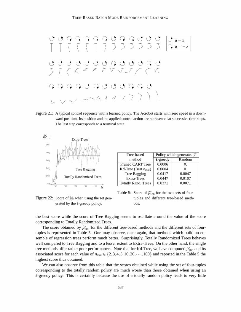
TREE-BASED BATCH MODE REINFORCEMENTLEARNING
u = 5u =−5
Figure 21: A typical control sequence with a learned policy. The Acrobot starts with zero speed in a down-ward position. Its position and the applied control action are represented at successive time steps.The last step corresponds to a terminal state.
10 30 50 70 90
0.02
0.02
0.03
0.04
0.05
0.0
Jµ∗N∞
N
Tree Bagging
Extra-Trees
Totally Randomized Trees
Figure 22: Score ofµ∗N when using the set gen-erated by theε-greedy policy.
Tree-basedmethod
Policy which generatesFε-greedy Random
Pruned CART Tree 0.0006 0.Kd-Tree (Bestnmin) 0.0004 0.
Tree Bagging 0.0417 0.0047Extra-Trees 0.0447 0.0107
Totally Rand. Trees 0.0371 0.0071
Table 5: Score ofµ∗100 for the two sets of four-tuples and different tree-based meth-ods.
the best score while the score of Tree Bagging seems to oscillate around thevalue of the scorecorresponding to Totally Randomized Trees.
The score obtained by ˆµ∗100 for the different tree-based methods and the different sets of four-tuples is represented in Table 5. One may observe, once again, that methods which build an en-semble of regression trees perform much better. Surprisingly, Totally Randomized Trees behaveswell compared to Tree Bagging and to a lesser extent to Extra-Trees. On the other hand, the singletree methods offer rather poor performances. Note that for Kd-Tree,we have computed ˆµ∗100 and itsassociated score for each value ofnmin∈ {2,3,4,5,10,20, · · · ,100} and reported in the Table 5 thehighest score thus obtained.
We can also observe from this table that the scores obtained while using the set of four-tuplescorresponding to the totally random policy are much worse than those obtained when using anε-greedy policy. This is certainly because the use of a totally random policy leads to very little
537
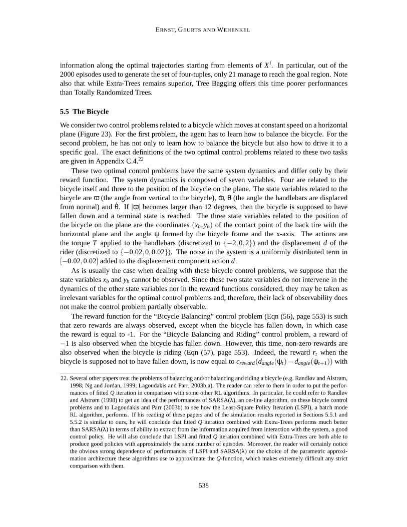
ERNST, GEURTS AND WEHENKEL
information along the optimal trajectories starting from elements ofXi . In particular, out of the2000 episodes used to generate the set of four-tuples, only 21 manage toreach the goal region. Notealso that while Extra-Trees remains superior, Tree Bagging offers this timepoorer performancesthan Totally Randomized Trees.
5.5 The Bicycle
We consider two control problems related to a bicycle which moves at constant speed on a horizontalplane (Figure 23). For the first problem, the agent has to learn how to balance the bicycle. For thesecond problem, he has not only to learn how to balance the bicycle but alsohow to drive it to aspecific goal. The exact definitions of the two optimal control problems related to these two tasksare given in Appendix C.4.22
These two optimal control problems have the same system dynamics and differonly by theirreward function. The system dynamics is composed of seven variables. Four are related to thebicycle itself and three to the position of the bicycle on the plane. The state variables related to thebicycle areω (the angle from vertical to the bicycle),ω, θ (the angle the handlebars are displacedfrom normal) andθ. If |ω| becomes larger than 12 degrees, then the bicycle is supposed to havefallen down and a terminal state is reached. The three state variables relatedto the position ofthe bicycle on the plane are the coordinates(xb,yb) of the contact point of the back tire with thehorizontal plane and the angleψ formed by the bicycle frame and the x-axis. The actions arethe torqueT applied to the handlebars (discretized to{−2,0,2}) and the displacementd of therider (discretized to{−0.02,0,0.02}). The noise in the system is a uniformly distributed term in[−0.02,0.02] added to the displacement component actiond.
As is usually the case when dealing with these bicycle control problems, we suppose that thestate variablesxb andyb cannot be observed. Since these two state variables do not intervene in thedynamics of the other state variables nor in the reward functions considered, they may be taken asirrelevant variables for the optimal control problems and, therefore, their lack of observability doesnot make the control problem partially observable.
The reward function for the “Bicycle Balancing” control problem (Eqn (56), page 553) is suchthat zero rewards are always observed, except when the bicycle has fallen down, in which casethe reward is equal to -1. For the “Bicycle Balancing and Riding” control problem, a reward of−1 is also observed when the bicycle has fallen down. However, this time, non-zero rewards arealso observed when the bicycle is riding (Eqn (57), page 553). Indeed, the rewardrt when thebicycle is supposed not to have fallen down, is now equal tocreward(dangle(ψt)−dangle(ψt+1)) with
22. Several other papers treat the problems of balancing and/or balancing and riding a bicycle (e.g. Randløv and Alstrøm,1998; Ng and Jordan, 1999; Lagoudakis and Parr, 2003b,a). Thereader can refer to them in order to put the perfor-mances of fittedQ iteration in comparison with some other RL algorithms. In particular, he couldrefer to Randløvand Alstrøm (1998) to get an idea of the performances of SARSA(λ), an on-line algorithm, on these bicycle controlproblems and to Lagoudakis and Parr (2003b) to see how the Least-Square Policy Iteration (LSPI), a batch modeRL algorithm, performs. If his reading of these papers and of the simulation results reported in Sections 5.5.1 and5.5.2 is similar to ours, he will conclude that fittedQ iteration combined with Extra-Trees performs much betterthan SARSA(λ) in terms of ability to extract from the information acquired from interaction with the system, a goodcontrol policy. He will also conclude that LSPI and fittedQ iteration combined with Extra-Trees are both able toproduce good policies with approximately the same number of episodes. Moreover, the reader will certainly noticethe obvious strong dependence of performances of LSPI and SARSA(λ) on the choice of the parametric approxi-mation architecture these algorithms use to approximate theQ-function, which makes extremely difficult any strictcomparison with them.
538
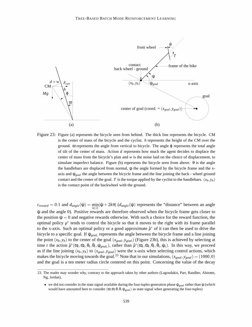
TREE-BASED BATCH MODE REINFORCEMENTLEARNING
ϕh
d+w FcenCM
ω
Mg
x-axis
ψ
ψgoal
contact
θ
T
front wheel
back wheel - ground
goal
(xb,yb)
frame of the bike
center of goal (coord. =(xgoal,ygoal))
(a) (b)
Figure 23: Figure (a) represents the bicycle seen from behind. The thick line represents the bicycle. CMis the center of mass of the bicycle and the cyclist.h represents the height of the CM over theground. ω represents the angle from vertical to bicycle. The angleϕ represents the total angleof tilt of the center of mass. Actiond represents how much the agent decides to displace thecenter of mass from the bicycle’s plan andw is the noise laid on the choice of displacement, tosimulate imperfect balance. Figure (b) represents the bicycle seen from above.θ is the anglethe handlebars are displaced from normal,ψ the angle formed by the bicycle frame and the x-axis andψgoal the angle between the bicycle frame and the line joining the back - wheel groundcontact and the center of the goal.T is the torque applied by the cyclist to the handlebars.(xb,yb)
is the contact point of the backwheel with the ground.
creward = 0.1 anddangle(ψ) = mink∈Z
|ψ + 2kπ| (dangle(ψ) represents the “distance” between an angle
ψ and the angle 0). Positive rewards are therefore observed when the bicycle frame gets closer tothe positionψ = 0 and negative rewards otherwise. With such a choice for the reward function, theoptimal policyµ∗ tends to control the bicycle so that it moves to the right with its frame parallelto the x-axis. Such an optimal policy or a good approximate ˆµ∗ of it can then be used to drive thebicycle to a specific goal. Ifψgoalt represents the angle between the bicycle frame and a line joiningthe point(xb,yb) to the center of the goal(xgoal,ygoal) (Figure 23b), this is achieved by selecting attime t the actionµ∗(ωt , ωt ,θt , θt ,ψgoalt ), rather than ˆµ∗(ωt , ωt ,θt , θt ,ψt). In this way, we proceedas if the line joining(xb,yb) to (xgoal,ygoal) were the x-axis when selecting control actions, whichmakes the bicycle moving towards the goal.23 Note that in our simulations,(xgoal,ygoal) = (1000,0)and the goal is a ten meter radius circle centered on this point. Concerning thevalue of the decay
23. The reader may wonder why, contrary to the approach taken by other authors (Lagoudakis, Parr, Randløv, Alstrøm,Ng, Jordan),
• we did not consider in the state signal available during the four-tuples generation phaseψgoal rather thanψ (whichwould have amounted here to consider(ω, ω,θ, θ,ψgoal) as state signal when generating the four-tuples)
539
ERNST, GEURTS AND WEHENKEL
factorγ, it has been chosen for both problems equal to 0.98. The influence ofγ andcreward on thetrajectories for the “Bicycle Balancing and Riding” control problem will be discussed later.
All episodes used to generate the four-tuples start from a state selected at random in
{(ω, ω,θ, θ,xb,yb,ψ) ∈ R7|ψ ∈ [−π,π]andω = ω = θ = θ = xb = yb = 0},
and end when a terminal state is reached, i.e. when the bicycle is supposed tohave fallen down. Thepolicy considered during the four-tuples generation phase is a policy thatselects at each instant anaction at random inU .
For both optimal control problems, the setXi considered for the score computation (Section5.1.2) is:
Xi = {(ω, ω,θ, θ,xb,yb,ψ) ∈ R7|ψ ∈ {−π,−3π
4, · · · ,π}andω = ω = θ = θ = xb = yb = 0}.
Sinceψ andψ+2kπ (k∈Z) are equivalent from a physical point of view, in our simulations wehave modified each value ofψ observed by a factor 2kπ in order to guarantee that it always belongsto [−π,π].
5.5.1 THE “B ICYCLE BALANCING ” CONTROL PROBLEM
To generate the four-tuples, we have considered 1000 episodes. Thecorresponding setF is com-posed of 97,969 four-tuples. First, we discuss the results obtained by Extra-Trees (nmin = 4, K = 7,M = 50)24 and then we assess the performances of the other tree-based methods.
Figure 24a represents the evolution of the score of the policies ˆµ∗N with N when using Extra-Trees. To assess the quality of a policyµ, we use also another criterion than the score. For thiscriterion, we simulate for eachx0 ∈ Xi ten times the system with the policyµ, leading to a total of90 trajectories. If no terminal state has been reached beforet = 50,000, that is if the policy was ableto avoid crashing the bicycle during 500 seconds (the discretization time step is0.01 second), we saythat the trajectory has been successful. On Figure 24c we have represented for the different policiesµ∗N the number of successful trajectories among the 90 simulated. Remark that if from N = 60the score remains really close to zero, polices ˆµ∗60 and µ∗70 do not produce as yet any successfultrajectories, meaning that the bicycle crashes for large values oft even if these are smaller than
• the reward function for the bicycle balancing and riding control problem does not give directly information aboutthe direction to the goal (which would have led here to observe att + 1 the rewardcreward(dangle(ψgoalt )−dangle(ψgoalt+1))).
We did not choose to proceed like this becauseψgoalt+1 depends not only onψgoalt andθt but also onxbt andybt .Therefore, since we suppose that the coordinates of the back tire cannot be observed, the optimal control problemswould have been partially observable if we had replacedψ by ψgoal in the state signal and the reward function.Although in our simulations this does not make much difference sinceψ ' ψgoal during the four-tuples generationphases, we prefer to stick with fully observable systems in this paper.
24. When considering ensemble methods (Extra-Trees, Totally Randomized Trees, Tree Bagging) we always keep con-stant the value of these parameters. Since we are not dealing with a highly stochastic system, as for the case of the“Left or Right” control problem, we decided not to rely on the pruned version of these algorithms. However, wefound out that by developing the trees fully (nmin = 2), variance was still high. Therefore, we decided to use a largervalue fornmin. This value is equal to 4 and was leading to a good bias-variance tradeoff. Concerning the value ofK = 7, it is equal to the dimension of the input space, that is the dimension of the state signal(ω, ω,θ, θ,ψ) plus thedimension of the action space.
540

TREE-BASED BATCH MODE REINFORCEMENTLEARNING
Tree-based methodControl problem
BicycleBalancing
BicycleBalancing and Riding
Pruned CART Tree -0.02736 -0.03022Kd-Tree (Bestnmin∈ {2,3,4,5,10,20, · · · ,100}) -0.02729 -0.10865
Tree Bagging (nmin = 4, M = 50) 0 0.00062Extra-Trees (nmin = 4, K = 7, M = 50 ) 0 0.00157
Totally Randomized Trees (nmin = 4, M = 50) -0.00537 -0.01628
Table 6: Score ofµ∗300 for the “Balancing” and “Balancing and Riding” problems. Different tree-basedmethods are considered, with a 1000 episode based set of four-tuples.
50,000. Figure 24b gives an idea of the trajectories of the bicycle on the horizontal plane whenstarting from the different elements ofXi and being controlled by ˆµ∗300.
To assess the influence of the number of four-tuples on the quality of the policy computed, wehave drawn on Figure 24d the number of successful trajectories when different number of episodesare used to generateF . As one may see, by using Extra-Trees, from 300 episodes (' 10,000four-tuples) only successful trajectories are observed. Tree Bagging and Totally Randomized Treesperform less well. It should be noted that Kd-Tree and Pruned CART Tree were not able to pro-duce any successful trajectories, even for the largest set of four-tuples. Furthermore, the fact thatwe obtained some successful trajectories with Totally Randomized Trees is only because we havemodified the algorithm to avoid selection of tests according toψ, a state variable that plays for this“Bicycle Balancing” control problem the role of an irrelevant variable (ψ does not intervene in thereward function and does not influence the dynamics ofω, ω, θ, θ) (see also Section 5.3.5). Notethat the scores obtained by ˆµ∗300 for the different tree-based methods when considering the 97,969four-tuples are reported in the second column of Table 6.
5.5.2 THE “B ICYCLE BALANCING AND RIDING” CONTROL PROBLEM
To generate the four-tuples, we considered 1000 episodes that led to a set F composed of 97,241elements. First, we study the performances of Extra-Trees (nmin = 4, K = 7, M = 50). Figure 25arepresents the evolution of the score of ˆµ∗N with N. The final value of the score (score of ˆµ∗300) isequal to 0.00157.
As mentioned earlier, with the reward function chosen, the policy computed byour algorithmshould be able to drive the bicycle to the right, parallel to the x-axis, provided that the policy is agood approximation of the optimal policy. To assess this ability, we have simulated, for eachx0∈Xi ,the system with the policy ˆµ∗300 and have represented on Figure 25b the different trajectories of theback tire. As one may see, the policy tends indeed to drive the bicycle to the right, parallel to thex-axis. The slight shift that exists between the trajectories and the x-axis (the shift is less than 10degrees) could be reduced if more four-tuples were used as input of the fittedQ iteration algorithm.
Now, if rather than using the policy ˆµ∗300 with the state signal(ω, ω,θ, θ,ψ) we consider the statesignal (ω, ω,θ, θ,ψgoal), whereψgoal is the angle between the bicycle frame and the line joining(xb,yb) with (xgoal,ygoal), we indeed observe that the trajectories converge to the goal (see Figure25c). Under such conditions, by simulating from eachx0 ∈ Xi ten times the system over 50,000time steps, leading to a total of 90 trajectories, we observed that every trajectory managed to reach
541
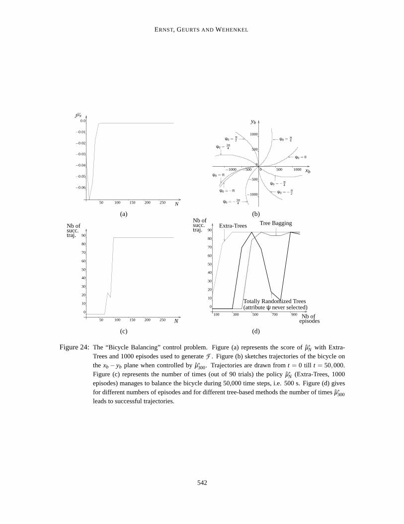
ERNST, GEURTS AND WEHENKEL
−0.06
−0.05
−0.04
−0.03
0.0
−0.01
−0.02
N
Jµ∗N
10050 150 200 250
−1000 −500 500 1000
−500
0
500
1000
−1000
xbψ0 = π
ψ0 =−π
yb
ψ0 =− π4
ψ0 =− π2
ψ0 = π4
ψ0 = 0
ψ0 =− 3π4
ψ0 = π2
ψ0 = 3π4
0
(a) (b)
10050 150 200 250
0
10
20
30
40
50
60
70
80
90
N
succ.Nb of
traj.
Totally Randomized Trees(attributeψ never selected)
100 300 500 700 900
0
10
20
30
40
50
60
70
80
90
Nb of
Nb ofepisodes
Extra-Trees Tree Baggingsucc.traj.
(c) (d)
Figure 24: The “Bicycle Balancing” control problem. Figure (a) represents the score of ˆµ∗N with Extra-Trees and 1000 episodes used to generateF . Figure (b) sketches trajectories of the bicycle onthe xb− yb plane when controlled by ˆµ∗300. Trajectories are drawn fromt = 0 till t = 50,000.Figure (c) represents the number of times (out of 90 trials) the policy µ∗N (Extra-Trees, 1000episodes) manages to balance the bicycle during 50,000 timesteps, i.e. 500 s. Figure (d) givesfor different numbers of episodes and for different tree-based methods the number of times ˆµ∗300
leads to successful trajectories.
542

TREE-BASED BATCH MODE REINFORCEMENTLEARNING
a 2 meter neighborhood of(xgoal,ygoal). Furthermore, every trajectory was able to reach the goal inless that 47,000 time steps. Note that, since the bicycle rides at constant speedv = 10
3.6 ' 2.77ms−1
and since the time discretization step is 0.01s, the bicycle does not have to cover a distance of morethat 1278mbefore reaching the goal while starting from any element ofXi .
It is clear that these good performances in terms of the policy ability to drive the bicycle to thegoal depend on the choice of the reward function. For example, if the sameexperience is repeatedwith creward chosen equal to 1 rather than 0.1 in the reward function, the trajectories lead rapidlyto a terminal state. This can be explained by the fact that, in this case, the largepositive rewardsobtained for moving the frame of the bicycle parallel to the x-axis lead to a control policy thatmodifies too rapidly the bicycle riding direction which tends to destabilize it. If now, the coefficientcreward is taken smaller than 0.1, the bicycle tends to turn more slowly and to take more time toreach the goal. This is illustrated on Figure 25d where a trajectory corresponding tocreward = 0.01is drawn together with a trajectory corresponding tocreward = 0.1. On this figure, we may alsoclearly observe that after leaving the goal, the control policies tend to drive again the bicycle to it.It should be noticed that the policy corresponding tocreward = 0.1 manages at each loop to bringthe bicycle back to the goal while it is not the case with the policy corresponding to creward = 0.01.Note that the coefficientγ influences also the trajectories obtained. For example, by takingγ = 0.95instead ofγ = 0.98, the bicycle crashes rapidly. This is due to the fact that a smaller value ofγ tendsto increase the importance of short-term rewards over long-term ones, which favors actions that turnrapidly the bicycle frame, even if they may eventually lead to a fall of the bicycle.
Rather than relying only on the score to assess the performances of a policy, let us now associateto a policy a value that depends on its ability to drive the bicycle to the goal within acertain timeinterval, when(ω, ω,θ, θ,ψgoal) is the state signal considered. To do so, we simulate from eachx0∈Xi ten times the system over 50,000 time steps and count the number of times the goal has beenreached. Figure 25e represents the “number of successful trajectories” obtained by ˆµ∗N for differentvalues ofN. Observe that 150 iterations of fittedQ iteration are needed before starting to observesome successful trajectories. Observe also that the “number of successful trajectories” sometimesdrops whenN increases, contrary to intuition. These drops are however not observed on the scorevalues (e.g. forN = 230, all 90 trajectories are successful and the score is equal to 0.00156, whilefor N = 240, the number of successful trajectories drops to 62 but the score increases to 0.00179).Additional simulations have shown that these sudden drops tend to disappear when using morefour-tuples.
Figure 25f illustrates the influence of the size ofF on the number of successful trajectories whenfitted Q iteration is combined with Extra-Trees. As expected, the number of successful trajectoriestends to increase with the number of episodes considered in the four-tuplesgeneration process.It should be noted that the other tree-based methods considered in this paper did not manage toproduce successful trajectories when only 1000 episodes are used togenerate the four-tuples. Thedifferent scores obtained by ˆµ∗300 when 1000 episodes are considered and for the different tree-basedmethods are gathered in Table 6, page 541. Using this score metric, Extra-Trees is the methodperforming the best, which is in agreement with the “number of successful trajectories” metric,followed successively by Tree Bagging, Totally Randomized Trees, Pruned CART Tree and Kd-Tree.
543
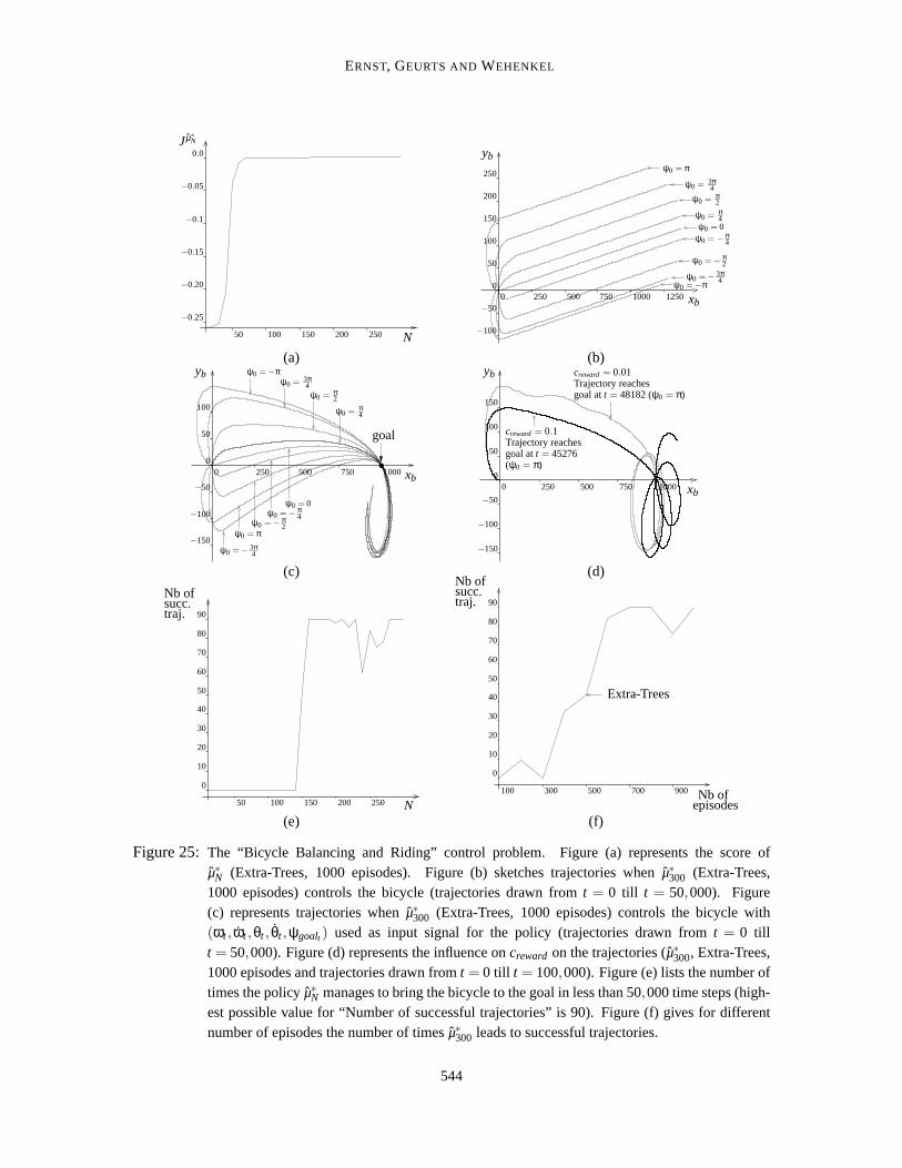
ERNST, GEURTS AND WEHENKEL
100 150 200 250
−0.25
−0.20
−0.15
−0.1
−0.05
0.0
N
Jµ∗N
50 −100
−50
0
50
100
150
200
250
0 250 500 750 1000 1250xb
ybψ0 = π
ψ0 = 3π4
ψ0 = π2
ψ0 = π4
ψ0 = 0ψ0 =− π
4
ψ0 =− π2
ψ0 =− 3π4ψ0 =−π
(a) (b)
goal
yb
0 250 500 750 1000
−100
−50
0
50
100
xb
−150ψ0 =− 3π
4
ψ0 = π
ψ0 =− π4
ψ0 =− π2
ψ0 = 0
ψ0 = π4
ψ0 = π2
ψ0 = 3π4
ψ0 =−π
0 250 500 750 1000
−150
−100
50
100
150
yb
xb
creward = 0.01Trajectory reachesgoal att = 48182 (ψ0 = π)
creward = 0.1Trajectory reaches
(ψ0 = π)goal att = 45276
0
−50
(c) (d)
10050 150 200 250
0
10
20
30
40
50
60
70
80
90
N
Nb ofsucc.traj.
100 300 500 700 900
0
10
20
30
40
50
60
70
80
90
Nb of
Nb ofepisodes
Extra-Trees
succ.traj.
(e) (f)
Figure 25: The “Bicycle Balancing and Riding” control problem. Figure(a) represents the score ofµ∗N (Extra-Trees, 1000 episodes). Figure (b) sketches trajectories when ˆµ∗300 (Extra-Trees,1000 episodes) controls the bicycle (trajectories drawn from t = 0 till t = 50,000). Figure(c) represents trajectories when ˆµ∗300 (Extra-Trees, 1000 episodes) controls the bicycle with(ωt , ωt ,θt , θt ,ψgoalt ) used as input signal for the policy (trajectories drawn fromt = 0 tillt = 50,000). Figure (d) represents the influence oncreward on the trajectories (ˆµ∗300, Extra-Trees,1000 episodes and trajectories drawn fromt = 0 till t = 100,000). Figure (e) lists the number oftimes the policy ˆµ∗N manages to bring the bicycle to the goal in less than 50,000 time steps (high-est possible value for “Number of successful trajectories”is 90). Figure (f) gives for differentnumber of episodes the number of times ˆµ∗300 leads to successful trajectories.
544
TREE-BASED BATCH MODE REINFORCEMENTLEARNING
5.6 Conclusion of the Experiments
We discuss in this section the main conclusions that may be drawn from the simulation resultspreviously reported.
5.6.1 INFLUENCE OF THETREE-BASED METHODS
Let us analyze the results of our experiments in the light of the classification given in Table 1.
Single trees vs ensembles of trees.Whatever the set of four-tuples used, the top score has alwaysbeen reached by a method building an ensemble of regression trees, and furthermore, the larger thestate space, the better these regression tree ensemble methods behave compared to methods buildingonly one single tree. These results are in agreement with previous work in reinforcement learningwhich suggests that multi-partitioning of the state space is leading to better function approxima-tors than single partitioning.25 They are also in agreement with the evaluation of these ensemblealgorithms on many standard supervised learning problems (classification and regression), wheretree-based ensemble methods typically significantly outperform single trees (Geurts et al., 2004).
However, from the viewpoint of computational requirements, we found that ensemble methodsare clearly more demanding, both in terms of computing times and memory requirements for thestorage of models.
Kernel-based vs non kernel-based methods.Among the single tree methods, Pruned CARTTree, which adapts the tree structure to the output variable, offers typically the same performancesas Kd-Tree, except in the case of irrelevant variables where it is significantly more robust. Amongthe tree-based ensemble methods, Extra-Trees outperforms Totally Randomized Trees in all cases.On the other hand, Tree Bagging is generally better than the Totally Randomized Trees, exceptwhen dealing with very small numbers of samples, where the bootstrap resampling appears to bepenalizing. These experiments thus show that tree-based methods that adapt their structure to thenew output at each iteration usually provide better results than methods that do not (that we namekernel-based). Furthermore, the non kernel-based tree-based algorithms are much more robust tothe presence of irrelevant variables thanks to their ability to filter out tests involving these variables.
A drawback of non kernel-based methods is that they do not guarantee convergence. However,with the Extra-Trees algorithm, even if the sequence was not converging,the policy quality wasoscillating only moderately around a stable value and even when at its lowest, itwas still superiorto the one obtained by the kernel-based methods ensuring the convergence of the algorithm. Fur-thermore, if really required, convergence to a stable approximation may always be provided in anad hoc fashion, for example by freezing the tree structures after a certain number of iterations andthen only refreshing predictions at terminal nodes.
5.6.2 PARAMETRIC VERSUSNON-PARAMETRIC SUPERVISEDLEARNING METHOD
FittedQ iteration has been used in our experiments with non-parametric supervised learning meth-ods (kNN, tree-based methods) and parametric supervised learning methods (basis function methodswith piecewise-constant or piecewise-linear grids as approximation architectures).
25. See e.g. Sutton (1996); Sutton and Barto (1998), where the authors show that by overlaying several shifted tilingsof the state space (type of approximation architecture known as CMACs),good function approximators could beobtained.
545

ERNST, GEURTS AND WEHENKEL
It has been shown that the parametric supervised learning methods, compared to the non-parametric ones, were not performing well. The main reason is the difficulty toselect a priori theshape of the parametric approximation architecture that may lead to some good results. It shouldalso be stressed that divergence to infinity of the fittedQ iteration has sometimes been observedwhen piecewise-linear grids were the approximation architectures considered.
5.6.3 FITTED Q ITERATION VERSUSON-L INE ALGORITHMS
An advantage of fittedQ iteration over on-line algorithms is that it can be combined with some non-parametric function approximators, shown to be really efficient to generalize the information. Wehave also compared the performances of fittedQ iteration andQ-learning for some a priori givenparametric approximation architectures. In this context, we found out that when the approximationarchitecture used was chosen so as to avoid serious convergence problems of the fittedQ iterationalgorithm, then this latter was also performing much better thanQ-learning on the same architecture.
6. Conclusions and Future Work
In this paper, we have considered a batch mode approach to reinforcement learning, which consistsof reformulating the reinforcement learaning problem as a sequence of standard supervised learningproblems. After introducing thefitted Q iteration algorithmwhich formalizes this framework, wehave studied the properties and performances of the algorithm when combined with three classicaltree-based methods (Kd-Trees, CART Trees, Tree Bagging) and two newly proposed tree-basedensemble methods namely Extra-Trees and Totally Randomized Trees.
Compared with grid-based methods on low-dimensional problems, as well as with kNN andsingle tree-based methods in higher dimensions, we found out that the fittedQ iteration algorithmwas giving excellent results when combined with any one of the consideredtree-based ensemblemethods (Extra-Trees, Tree Bagging and Totally Randomized Trees). Onthe different cases studied,Extra-Treeswas the supervised learning method able to extract at best information froma set of four-tuples. It is also faster than Tree Bagging and was performing significantlybetter than this latteralgorithm, especially on the higher dimensional problems and on low-dimensional problems withsmall sample sizes. We also found out that fittedQ iteration combined with tree-based methodswas performing much better thanQ-learning combined with piecewise-constant or piecewise-lineargrids.
Since Extra-Trees and Tree Bagging, the two best performing supervised learning algorithms,readjust their approximation architecture to the output variable at each iteration, they do not en-sure the convergence of the fittedQ iteration algorithm. However, and contrary to many parametricapproximation schemes, they do not lead to divergence to infinity problems. The convergence prop-erty is satisfied by theTotally Randomized Treesbecause their set of trees is frozen at the beginningof the iteration. They perform however less well than Extra-Trees and Tree Bagging, especially inthe presence of irrelevant variables. They are nevertheless better than some other methods that alsoensure the convergence of the sequence, likekNN kernel methods and piecewise-constant grids, interms of performances as well as scalability to large numbers of variables and four-tuples. Withinthis context, it would be worth to study versions of Extra-Trees and Tree Bagging which wouldfreeze their trees at some stage of the iteration process, and thus recover the convergence property.
From a theoretical point of view, it would certainly be very interesting to further study the con-sistency of the fittedQ iteration algorithm, in order to determine general conditions under which the
546
TREE-BASED BATCH MODE REINFORCEMENTLEARNING
algorithm converges to an optimal policy when the number of four-tuples collected grows to infinity.With this in mind, one could possibly seek inspiration in the work of Ormoneit and Sen (2002) andOrmoneit and Glynn (2002), who provide consistency conditions for kernel-based supervised learn-ing methods within the context of fittedQ iteration, and also in some of the material published in thesupervised learning literature (e.g. Lin and Jeon, 2002; Breiman, 2000). More specifically, furtherinvestigation in order to characterize ensembles of regression trees with respect to consistency isparticularly wishful, because of their good practical performances.
In this paper, the score associated to a test node of a tree was the relativevariance reduction.Several authors who adapted regression trees in other ways to reinforcement learning have sug-gested the use of other score criteria for example based on the violation of the Markov assumption(McCallum, 1996; Uther and Veloso, 1998) or on the combination of several error terms like thesupervised, the Bellman, and the advantage error terms (Wang and Diettrich, 1999). Investigatingthe effect of such score measures within the fittedQ iteration framework is another interesting topicof research.
While the fittedQ iteration algorithm used with tree-based ensemble methods reveals itself tobe very effective to extract relevant information from a set of four-tuples, it has nevertheless onedrawback: with increasing number of four-tuples, it involves a superlinear increase in computingtime and a linear increase in memory requirements. Although our algorithms offera very goodaccuracy/efficiency tradeoff, we believe that further research should explore different ways to try toimprove the computational efficiency and the memory usage, by introducing algorithm modifica-tions specific to the reinforcement learning context.
Acknowledgments
Damien Ernst and Pierre Geurts gratefully acknowledge the financial support of the Belgian Na-tional Fund of Scientific Research (FNRS). The authors thank the action editor Michael Littmanand the three anonymous reviewers for their many suggestions for improvingthe quality of themanuscript. They are also very grateful to Bruno Scherrer for reviewing an earlier version of thiswork, to Mania Pavella for her helpful comments and to Michail Lagoudakis for pointing out rele-vant information about the bicycle control problems.
Appendix A. Extra-Trees Induction Algorithm
The procedure used by the Extra-Trees algorithm to build a tree from a training set is described inFigure 26. This algorithm has two parameters:nmin, the minimum number of elements required tosplit a node andK, the maximum number of cut-directions evaluated at each node. IfK = 1 thenat each test node the cut-direction and the cut-point are chosen totally at random. If in additionthe condition (iii) is dropped, then the tree structure is completely independentof the output valuesfound in theT S , and the algorithm generatesTotally Randomized Trees.The score measure used is the relative variance reduction. In other words, if T S l (resp. T S r )denotes the subset of cases fromT S such that[i j < t] (resp. [i j ≥ t]), then the Score is defined asfollows:
Score([i j < t],T S) =var(o|T S)− #T S l
#T Svar(o|T S l )− #T S r
#T Svar(o|T S r)
var(o|T S), (25)
547

ERNST, GEURTS AND WEHENKEL
Build a tree(T S )Input: a training setT S
Output: a treeT;
• If
(i) #T S < nmin, or
(ii) all input variables are constant inT S , or
(iii) the output variable is constant over theT S ,
return a leaf labeled by the average value1#T S ∑l ol .
• Otherwise:
1. Let [i j < t j ] = Find a test(T S).
2. SplitT S into T S l andT S r according to the test[i j < t].
3. Build Tl = Build a tree(T S l ) andTr = Build a tree(T S r) from these subsets;
4. Create a node with the test[i j < t j ], attachTl andTr as left and right subtrees of thisnode and return the resulting tree.
Find a test(T S )Input: a training setT S
Output: a test[i j < t j ]:
1. SelectK inputs,{i1, ..., iK}, at random, without replacement, among all (non constant) inputvariables.
2. Fork going from 1 toK:
(a) Compute the maximal and minimal value ofik in T S , denoted respectivelyiT Sk,min and
iT Sk,max.
(b) Draw a discretization thresholdtk uniformly in ]iT Sk,min, i
T Sk,max]
(c) Compute the scoreSk = Score([ik < tk],T S)
3. Return a test[i j < t j ] such thatSj = maxk=1,...,K Sk.
Figure 26: Procedure used by the Extra-Trees algorithm to build a tree. The Totally RandomizedTreesalgorithm is obtained from this algorithm by settingK = 1 and by dropping thestopping condition (iii).
548

TREE-BASED BATCH MODE REINFORCEMENTLEARNING
wherevar(o|X ) is the variance of the outputo in the training setX .
Appendix B. Convergence of the Sequence ofQN-Functions
Theorem 1 If the fitted Q iteration algorithm is combined with a supervised learning method whichproduces a model of the type (17) with the kernel kT S being the same from one iteration to the otherand satisfying the normalizing condition (18), then the sequence ofQN-functions converges.
Proof The proof is adapted in a straightforward way from Ormoneit and Sen (2002) to the fact thatthe kernelkT S((x
lt ,u
lt),(x,u)) may not be decomposed here into the productk′(xl
t ,x)δ(ult ,u).
Let us first observe that in such conditions, the sequence of functionscomputed by the fittedQiteration algorithm is determined by the recursive equation:
QN(x,u) =#F
∑l=1
kT S ((xlt ,u
lt),(x,u))[r l
t + γmaxu′∈U
QN−1(xlt+1,u
′)], ∀N > 0 (26)
with Q0(x,u) = 0 ∀(x,u) ∈ X×U . Equation (26) may be rewritten:
QN = HQN−1 (27)
whereH is an operator mapping any functionK : X×U → R and defined as follows:
(HK)(x,u) =#F
∑l=1
kT S ((xlt ,u
lt),(x,u))[r l
t + γmaxu′∈U
K(xlt+1,u
′)]. (28)
This operator is a contraction on the Banach space of functions defined over X×U and the supre-mum norm. Indeed, we have:
‖HK− HK‖∞ = γ max(x,u)∈X×U
|#F
∑l=1
kT S ((xlt ,u
lt),(x,u))[max
u′∈UK(xl
t+1,u′)−max
u′∈UK(xl
t+1,u′)]|
≤ γ max(x,u)∈X×U
|[#F
∑l=1
kT S((xlt ,u
lt),(x,u))max
u′∈U[K(xl
t+1,u′)−K(xl
t+1,u′)]|
≤ γ max(x,u)∈X×U
|K(x,u)−K(x,u)|
= γ‖K−K‖∞
< ‖K−K‖∞.
By virtue of the fixed-point theorem (Luenberger, 1969) the sequence converges, independentlyof the initial conditions, to the functionQ : X×U → R which is unique solution of the equationQ = HQ.
Appendix C. Definition of the Benchmark Optimal Control Probl ems
We define in this section the different optimal control problems used in our experiments. Simulators,additional documentation and sets of four-tuples are available upon request.
549

ERNST, GEURTS AND WEHENKEL
C.1 The “Left or Right” Control Problem
System dynamics:
xt+1 = xt +ut +wt
wherew is drawn according the standard (zero mean, unit variance) Gaussian distribution.If xt+1 is such that|xt+1|> 10 or|xt+1|< 0 then a terminal state is reached.State space:The state spaceX is composed of{x∈ R|x∈ [0,10]} and of a terminal state.Action space:The action spaceU = {−2,2}.Reward function: The reward functionr(x,u,w) is defined through the following expression:
r(xt ,ut ,wt) =
0 if xt+1 ∈ [0,10]
50 if xt+1 < 0
100 if xt+1 > 10.
(29)
Decay factor: The decay factorγ is equal to 0.75.
C.2 The “Car on the Hill” Control Problem
System dynamics:The system has a continuous-time dynamics described by these two differentialequations:
p = s (30)
s =u
m(1+Hill ′(p)2)− gHill ′(p)
1+Hill ′(p)2 −s2Hill ′(p)Hill ′′(p)
1+Hill ′(p)2 (31)
wheremandg are parameters equal respectively to 1 and 9.81 and whereHill (p) is a function ofpdefined by the following expression:
Hill (p) =
p2 + p if p < 0p√
1+5p2if p≥ 0.
(32)
The discrete-time dynamics is obtained by discretizing the time with the time betweent andt + 1chosen equal to 0.100s.If pt+1 andst+1 are such that|pt+1|> 1 or |st+1|> 3 then a terminal state is reached.State space:The state spaceX is composed of{(p,s) ∈ R
2| |p| ≤ 1and|s| ≤ 3} and of a terminalstate.X \{terminal state} is represented on Figure 8a.Action space:The action spaceU = {−4,4}.Reward function: The reward functionr(x,u) is defined through the following expression:
r(xt ,ut) =
−1 if pt+1 <−1 or |st+1|> 3
1 if pt+1 > 1 and |st+1| ≤ 3
0 otherwise.
(33)
Decay factor: The decay factorγ has been chosen equal to 0.95.Integration: The dynamical system is integrated by using an Euler method with a 0.001s integra-tion time step.
550

TREE-BASED BATCH MODE REINFORCEMENTLEARNING
Remark: This “Car on the Hill” problem is similar to the one found in Moore and Atkeson (1995)
except that the term− s2Hill ′(p)Hill ′′(p)1+Hill ′(p)2 is not neglected here in the system dynamics.
Variants of the control problem: In our experiments, we have also considered two other variantsof this problem:
• The “Car on the Hill” with irrelevant variables:some irrelevant variables are added to thestate vector. The value of an irrelevant variable at timet is determined by drawing at randoma number in[−2,2] with a uniform probability (used in Section 5.3.5).
• The “Car on the Hill” with continuous action space:the action space is not yet discreteanymore. It is continuous and equal to[−4,4] (used in Section 5.3.7).
C.3 The “Acrobot Swing Up” Control Problem
System dynamics:The system has a continuous-time dynamics described by these two second-order differential equations (taken from Yoshimoto et al., 1999):
d11θ1 +d12θ2 +c1 +φ1 = −µ1θ1 (34)
d12θ1 +d22θ2 +c2 +φ2 = u−µ2θ2 (35)
(36)
where
d11 = M1L21 +M2(L
21 +L2
2 +2L1L2cos(θ2)) (37)
d22 = M2L22 (38)
d12 = M2(L22 +L1L2cos(θ2)) (39)
c1 = −M2L1L2θ2(2θ1 + θ2sin(θ2)) (40)
c2 = M2L1L2θ12sin(θ2) (41)
φ1 = (M1L1 +M2L1)gsin(θ1)+M2L2gsin(θ1 +θ2) (42)
φ2 = M2L2gsin(θ1 +θ2). (43)
M1 (M2), L1 (L2) andµ1 (µ2) are the mass, length, and friction, respectively, of the first (second)link. θ1 is the angle of the first link from a downward position andθ2 is the angle of the secondlink from the direction of the first link (Figure 20).θ1 andθ2 are the angular velocities of the firstand second links, respectively. The system has four continuous state variablesx = (θ1,θ2, θ1, θ2).The physical parameters have been chosen equal toM1 = M2 = 1.0, L1 = L2 = 1.0, µ1 = µ2 = 0.01,g = 9.81.The discrete-time dynamics is obtained by discretizing the time with the time betweent andt + 1chosen equal to 0.100s.Let us denote byO the set composed of the statesx = ((2∗k+1)∗π,0,0,0) k∈ Z and byd(x,O)the value min
o∈O‖x−o‖.
If xt+1 is such thatd(xt+1,O) < 1 then a terminal state is reached.State space:The state space is composed of{x∈ R
4|d(x,O)≥ 1} and of a terminal state.Action space:The action spaceU = {−5,5}.
551
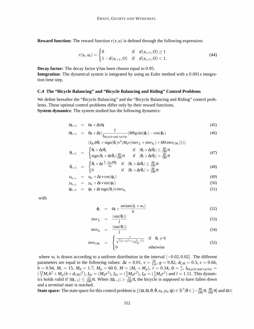
ERNST, GEURTS AND WEHENKEL
Reward function: The reward functionr(x,u) is defined through the following expression:
r(xt ,ut) =
{
0 if d(xt+1,O)≥ 1
1−d(xt+1,O) if d(xt+1,O) < 1.(44)
Decay factor: The decay factorγ has been chosen equal to 0.95.Integration: The dynamical system is integrated by using an Euler method with a 0.001s integra-tion time step.
C.4 The “Bicycle Balancing” and “Bicycle Balancing and Riding” Control Problems
We define hereafter the “Bicycle Balancing” and the “Bicycle Balancing and Riding” control prob-lems. These optimal control problems differ only by their reward functions.System dynamics: The system studied has the following dynamics:
ωt+1 = ωt +∆tωt (45)
ωt+1 = ωt +∆t(1
Ibicycle and cyclist(Mhgsin(ϕt)−cos(ϕt) (46)
(Idcσθt +sign(θt)v2(Mdr(invr ft + invrbt )+MhinvrCMt ))))
θt+1 =
{
θt +∆tθt if |θt +∆tθt | ≤ 80180π
sign(θt +∆tθt)80180π if |θt +∆tθt |> 80
180π(47)
θt+1 =
{
θt +∆t T−IdvσωtIdl
if |θt +∆tθt | ≤ 80180π
0 if |θt +∆tθt |> 80180π
(48)
xbt+1 = xbt +∆t vcos(ψt) (49)
ybt+1 = ybt +∆t vsin(ψt) (50)
ψt+1 = ψt +∆t sign(θt)v invrbt (51)
with
ϕt = ωt +arctan(dt +wt)
h(52)
invr ft =|sin(θt)|
l(53)
invrbt =| tan(θt)|
l(54)
invrCMt =
1√((l−c)2+( 1
invrbt)2)
if θt 6= 0
0 otherwise(55)
wherewt is drawn according to a uniform distribution in the interval[−0.02,0.02]. The differentparameters are equal to the following values:∆t = 0.01, v = 10
3.6, g = 9.82, dCM = 0.3, c = 0.66,h = 0.94, Mc = 15, Md = 1.7, Mp = 60.0, M = (Mc + Mp), r = 0.34, σ = v
r , Ibicycle and cyclist=(13
3 Mch2 +Mp(h+dCM)2), Idc = (Mdr2), Idv = (32Mdr2), Idl = (1
2Mdr2) andl = 1.11. This dynam-ics holds valid if|ωt+1| ≤ 12
180π. When|ωt+1| > 12180π, the bicycle is supposed to have fallen down
and aterminal stateis reached.State space:The state space for this control problem is{(ω, ω,θ, θ,xb,yb,ψ)∈R
7|θ∈ [− 80180π,
80180π] andω∈
552
TREE-BASED BATCH MODE REINFORCEMENTLEARNING
[− 12180π,
12180π]} plus aterminal state.
Action space:The action spaceU = {(d,T) ∈ {−0.02,0,0.02}×{−2,0,2}}. U is composed of 9elements.Reward functions: The reward function for the “Bicycle Balancing” control problem is definedhereafter:
r(xt ,ut ,wt) =
{
−1 if |ωt+1|> 12180π
0 otherwise.(56)
The reward function for “Bicycle Balancing and Riding” control problemis:
r(xt ,ut ,wt) =
{
−1 if |ωt+1|> 12180π
creward(dangle(ψt)−dangle(ψt+1)) otherwise(57)
wherecreward = 0.1 anddangle : R→ R such thatdangle(ψ) = mink∈Z
|ψ+2kπ|.Decay factor: The decay factorγ is equal to 0.98.Remark: The bicycle dynamics is based on the one found in Randløv and Alstrøm (1998) and intheir corresponding simulator available athttp://www.nbi.dk/∼randlov/bike.html.
References
D. Bagnell, S. Kakade, A. Y. Ng, and J. Schneider. Policy search by dynamic programming. InProceedings of Neural Information Processing Systems, 2003.
L. C. Baird. Residual algorithms: reinforcement learning with function approximation. In ArmandPrieditis and Stuart Russell, editors,Machine Learning: Proceedings of the Twelfth InternationalConference, pages 9–12, San Francisco, CA, July 1995. Morgan Kaufman.
R. Bellman.Dynamic Programming. Princeton University Press, 1957.
R. Bellman, R. Kalaba, and B. Kotkin. Polynomial approximation - a new computational techniquein dynamic programming: allocation processes.Mathematical Computation, 17:155–161, 1973.
J. A. Boyan. Technical update: least-squares temporal difference learning. Machine Learning, 49(2-3):233–246, 2002.
J. A. Boyan and A. W. Moore. Generalization in reinforcement learning:safely approximating thevalue function.Advances in Neural Information Processing Systems, 7:369–376, 1995.
L. Breiman. Bagging predictors.Machine Learning, 24(2):123–140, 1996.
L. Breiman. Some infinity theory for predictor ensembles. Technical Report 577, University ofCalifornia, Department of Statistics, 2000.
L. Breiman. Random forests.Machine Learning, 45(1):5–32, 2001.
L. Breiman, J. H. Friedman, R. A. Olsen, and C. J. Stone.Classification and Regression Trees.Wadsworth International (California), 1984.
553

ERNST, GEURTS AND WEHENKEL
D. Ernst. Near Optimal Closed-Loop Control. Application to Electric Power Systems. PhD thesis,University of Liege, Belgium, March 2003.
D. Ernst, P. Geurts, and L. Wehenkel. Iteratively extending time horizon reinforcement learning. InN. Lavra, L. Gamberger, and L. Todorovski, editors,Proceedings of the 14th European Confer-ence on Machine Learning, pages 96–107, Dubrovnik, Croatia, September 2003. Springer-VerlagHeidelberg.
D. Ernst, M. Glavic, P. Geurts, and L. Wehenkel. Approximate value iteration in the reinforce-ment learning context. Application to electrical power system control.To appear in IntelligentAutomation and Soft Computing, 2005.
P. Geurts, D. Ernst, and L. Wehenkel. Extremely randomized trees. Submitted, 2004.
G. J. Gordon. Online fitted reinforcement learning. InVFA workshop at ML-95, 1995a.
G. J. Gordon. Stable function approximation in dynamic programming. InProceedings of theTwelfth International Conference on Machine Learning, pages 261–268, San Francisco, CA,1995b. Morgan Kaufmann.
G. J. Gordon.Approximate Solutions to Markov Decision Processes. PhD thesis, Carnegie MellonUniversity, June 1999.
O. Hernandez-Lerma and B. Lasserre.Discrete-Time Markov Control Processes. Springer, New-York, 1996.
L. P. Kaelbling, M. L. Littman, and A. W. Moore. Reinforcement learning: asurvey. Journal ofArtificial Intelligence Research, 4:237–285, 1996.
S. Kakade and J. Langford. Approximately optimal approximate reinforcement learning. InPro-ceedings of the Nineteenth International Conference on Machine Learning, pages 267–274, 2002.
M. G. Lagoudakis and R. Parr. Least-squares policy iteration.Journal of Machine Learning Re-search, 4:1107–1149, 2003a.
M. G. Lagoudakis and R. Parr. Reinforcement learning as classification: leveraging modern classi-fiers. InProceedings of ICML 2003, pages 424–431, 2003b.
J. Langford and B. Zadrozny. Reducing T-step reinforcement learning to classification. Submitted,2004.
L. J. Lin. Reinforcement Learning for Robots Using Neural Networks. PhD thesis, Carnegie MellonUniversity, Pittsburgh, USA, 1993.
Y. Lin and Y. Jeon. Random forests and adaptive nearest neighbors. Technical Report 1005, De-partment of Statistics, University of Wisconsin, 2002.
D. G. Luenberger.Optimization by Vector Space Methods. Wiley, N.Y., 1969.
A. K. McCallum. Reinforcement Learning with Selective Perception and Hidden State. PhD thesis,University of Rochester, Rochester, New-York, 1996.
554

TREE-BASED BATCH MODE REINFORCEMENTLEARNING
A. W. Moore and C. G. Atkeson. Prioritized sweeping: reinforcement learning with less data andless real time.Machine Learning, 13:103–130, 1993.
A. W. Moore and C. G. Atkeson. The parti-game algorithm for variable resolution reinforcementlearning in multidimensional state-spaces.Machine Learning, 21(3):199–233, 1995.
A. Y. Ng and M. Jordan. PEGASUS: a policy search method for large MDPs and POMDPs. InProceedings of the Sixteenth Conference on Uncertainty in Artificial Intelligence, pages 406–415, 1999.
D. Ormoneit and P. Glynn. Kernel-based reinforcement learning in average-cost problems.IEEETransactions on Automatic Control, 47(10):1624–1636, 2002.
D. Ormoneit and S. Sen. Kernel-based reinforcement learning.Machine Learning, 49(2-3):161–178, 2002.
J. Randløv and P. Alstrøm. Learning to drive a bicycle using reinforcement learning and shaping.In Proceedings of the Fifteenth International Conference on Machine Learning, pages 463–471,San Francisco, CA, USA, 1998. Morgan Kaufmann Publishers Inc.
J. Rust. Using randomization to break the curse of dimensionality.Econometrica, 65(3):487–516,1997.
S. P. Singh, T. Jaakkola, and M. I. Jordan. Reinforcement learning with soft state aggregation. InG. Tesauro, D. S. Touretzky, and T. Leen, editors,Advances in Neural Information ProcessingSystems : Proceedings of the 1994 Conference, pages 359–368, Cambridge, MA, 1995. MITpress.
W. D. Smart and L. P. Kaelbling. Practical reinforcement learning in continuous spaces. InPro-ceedings of the Sixteenth International Conference on Machine Learning, pages 903–910, 2000.
M. W. Spong. Swing up control of the Acrobot. In1994 IEEE International Conference on Roboticsand Automation, pages 2356–2361, San Diego, CA, May 1994.
R. S. Sutton. Learning to predict by the method of temporal differences.Machine Learning, 3(1):9–44, 1988.
R. S. Sutton. Generalization in reinforcement learning: successful examples using sparse coarsecoding.Advances in Neural Information Processing Systems, 8:1038–1044, 1996.
R. S. Sutton and A. G. Barto.Reinforcement Learning, an Introduction. MIT Press, 1998.
J. N. Tsitsiklis. Asynchronous stochastic approximation andQ-learning.Machine Learning, 16(3):185–202, 1994.
J. N. Tsitsiklis and B. Van Roy. Feature-based methods for large-scale dynamic programming.Machine Learning, 22:59–94, 1996.
W. T. B. Uther and M. M. Veloso. Tree based discretization for continuous state space reinforcementlearning. InProceedings of AAAI-98, pages 769–774, 1998.
555

ERNST, GEURTS AND WEHENKEL
X. Wang and T. G. Diettrich. Efficient value function approximation using regression trees. InPro-ceedings of IJCAI-99 Workshop on Statistical Machine Learning for Large-Scale Optimization,Stockholm, Sweden, 1999.
C. J. C. H. Watkins.Learning from Delayed Rewards. PhD thesis, Cambridge University, Cam-bridge, England, 1989.
J. Yoshimoto, S. Ishii, and M. Sato. Application of reinforcement learning tobalancing Acrobot.In Proceedings of the 1999 IEEE International Conference on Systems, Man and Cybernetics,pages 516–521, 1999.
556