1

Transparency, Price Informativeness, Stock Return Synchronicity: Theory and Evidence1

Sudipto Dasgupta∗

Jie Gan+

Ning Gao#

This paper argues that, contrary to the conventional wisdom, stock return synchronicity (or R2) can increase when transparency improves. In a simple model, we show that, in more transparent environments, stock prices should be more informative about future events. Consequently, when the events actually happen in the future, there should be less “surprise”, i.e., there is less new information impounded into the stock price. Thus a more informative stock price today means higher return synchronicity in the future. We find empirical support for our theoretical predictions in three settings, namely firm age, seasoned equity issues, and listing of ADRs.

JEL Classification Code: G14, G39

Keywords: Stock return synchronicity, R2, Firm-specific return variation, Informativeness of stock prices, Transparency, Seasoned equity offering, Cross listing.

1 We thank Utpal Bhattacharya, Michael Brennan, Kalok Chan, Craig Doidge, Art Durnev, Robert Engle, Li Jin, Ernst Maug, Stewart Myers, Wei Jiang, Anil Makhija, Bill Megginson, Randall Morck, Mark Seasholes, Jeremy Stein, Martin Walker, Bernard Yeung and participants at the 2006 Financial Intermediation Research Society Conference and the 2006 WFA Conference for helpful comments and discussions. We are grateful to Hendrik Bessembinder (the editor) and two anonymous referees for their comments and suggestions which greatly improved the paper. ∗ Department of Finance, Hong Kong University of Science and Technology, Clear Water Bay, Kowloon, Hong Kong. Email: dasgupta@ust.hk. + Department of Finance, Hong Kong University of Science and Technology, Clear Water Bay, Kowloon, Hong Kong. Email: jgan@ust.hk. # The Manchester Accounting and Finance Group, Manchester Business School, the University of Manchester, Booth Street West, Manchester, M15 6PB, United Kingdom. Email: ning.gao@mbs.ac.uk.

2

Transparency, Price Informativeness, Stock Return Synchronicity: Theory and Evidence

Abstract

This paper argues that, contrary to the conventional wisdom, stock return synchronicity (or R2) can increase when transparency improves. In a simple model, we show that, in more transparent environments, stock prices should be more informative about future events. Consequently, when the events actually happen in the future, there should be less “surprise”, i.e., there is less new information impounded into the stock price. Thus a more informative stock price today means higher return synchronicity in the future. We find empirical support for our theoretical predictions in three settings, namely firm age, seasoned equity issues, and listing of ADRs.

JEL Classification Code: G14, G39

Keywords: Stock return synchronicity (R2), return synchronicity, Informativeness of stock

prices, Transparency, Seasoned equity offering, Cross listing.

3

I. Introduction Financial economists generally agree that in efficient markets, stock prices change to

reflect available information – either firm-specific or market-wide. Recent literature has

addressed the question of how a firm’s information environment (disclosure policy, analyst

following) or its institutional environment (property rights protection, quality of government,

legal origin) can affect the relative importance of firm-specific as opposed to market wide factors

(Jin and Myers (2006), Piotroski and Roulstone (2003), Chan and Hameed (2006), and Morck,

Yeung and Yu (2000)). This literature has taken the perspective that if the firm’s environment

causes stock prices to aggregate more firm-specific information, market factors should explain a

smaller proportion of the variation in stock returns. In other words, the stock return synchronicity

or R2 from a standard market model regression should be lower.

This perspective, while intuitive, is at odds with another equally intuitive implication of

market efficiency. In efficient markets, stock prices respond only to announcements that are not

already anticipated by the market. When the information environment surrounding a firm

improves and more firm-specific information is available, market participants are also able to

improve their predictions about the occurrence of future firm-specific events. As a result,

prevailing stock prices are likely to already “factor in” the likelihood of occurrence of these

events. When the events actually happen in the future, the market will not react to such news,

since there is little “surprise”. In other words, more informative stock prices today should be

associated with less firm-specific variation in stock prices in the future. Therefore, the return

synchronicity should be higher.

In this paper, we present a simple model to illustrate the point that a more transparent

information environment can lead to higher, rather than lower, stock return synchronicity. This is

because, for a more transparent firm, there is already more information available to market

participants, reducing the “surprise” from future announcements. In our model, we distinguish

between two types of firm-specific information. One pertains to time-varying firm

characteristics, reflecting the current state of the firm, such as next quarter’s earnings. The other

is time-invariant, such as managerial quality. 2 Stock return synchronicity can increase

2 Strictly speaking all firm characteristics are time varying in the very long run. Here we refer to those characteristics that do not change frequently or do not change much over time (so that they do not affect valuation significantly) as “time-invariant.”

4

subsequent to an improvement in transparency through disclosure of both types of information.

First, greater transparency can lead to early disclosure of time-variant information. This can

happen around major events such as seasoned equity issues (SEOs) or cross-listings, during

which a big chunk of information about future events is revealed. Thus when future events

actually happen, there is less “surprise” and hence less additional information to be incorporated

in the stock price, resulting in a higher return synchronicity.3 While the positive effect of greater

transparency on return synchronicity is most significant in the case of a one-time lumpy

disclosure, we show that it also holds in the more general setting with regular, early disclosure of

information. In particular, we show that in a dynamic setting, if at the beginning of every period,

outsiders get to know (one period ahead of time) some of the information that otherwise would

come out at the end of the period, the return synchronicity is actually higher.

The second channel through which greater transparency increases stock return

synchronicity is due to learning about time-invariant firm-specific characteristics, such as

managerial quality. In particular, better disclosure allows market participants to learn about time-

invariant firm fundamentals with greater precision (e.g., in the extreme case where the

fundaments are completely known, there is no new learning). Therefore, with more disclosure,

the priors about these fundamentals will be revised less drastically as new information comes in.

As a result, there will be less firm-specific variation in stock prices, i.e., the return synchronicity

will be higher.

We present three pieces of empirical evidence consistent with our model’s predictions.

We first provide evidence of learning about time-invariant firm-specific information. The idea is

that, as a firm becomes older, the market learns more about its time-invariant characteristics, e.g.,

the firm’s intrinsic quality. Therefore, return synchronicity should be higher for older firms,

since more of the (time-invariant) firm-specific information is already reflected in the stock

price. This prediction is strongly supported by the data.

Second and third, we exploit the fact that the effect of greater transparency on stock

return synchronicity is likely to be especially clear when the disclosure is “lumpy”, in the sense

that the market receives a big chunk of information relevant for future cash flows. Therefore, we

3 Shiller (1981) notes theoretically that if dividend news arrives in a lumpy and infrequent way, stock price volatility becomes lower. If much of the dividend news reflects firm specific information, one would also expect return synchronicity to become higher.

5

focus on seasoned equity offerings (SEOs) and cross-listings in the U.S.4 It is well known that

both events are associated with significant amounts of information disclosure and market

scrutiny (see e.g., Almazan et al. (2002) for SEO, and Lang et al. (2003) for ADR listings). Our

model suggests a dynamic response of return synchronicity to an improvement in the information

environment. At the time when new information is disclosed and impounded into stock prices,

the firm-specific return variation will increase, as suggested by conventional wisdom. However,

since a big chunk of relevant information is already reflected in stock prices, we would expect

the firm-specific return variation of SEO and cross-listed firms to be subsequently lower. This

dynamic response of the firm-specific return variation around seasoned equity issues and cross-

listing events is the main focus of our empirical exercise and we find strong support for it in the

data.5

Overall, in this paper, we make two contributions to the literature. First, we address the

literature on transparency, informativeness of stock prices, and stock return synchronicity by

arguing that a more transparent firm can have a higher return synchronicity, contrary to the

conventional wisdom. Therefore, our paper highlights that it is important to understand the

nature of information disclosure in trying to interpret any particular association (or its absence)

between transparency and stock return synchronicity. Second, we add to the growing literature

on information disclosure around security issuance events such as SEOs or ADRs by showing

that stock price synchronicity changes in a way that is consistent with lumpy information

disclosure associated with these events.

The rest of the paper is organized as follows. Section II reviews related literature. Section

III presents the model. Section IV reports the empirical findings and Section V concludes.

II. Related Literature A. Stock Return Synchronicity (R2)

A recent literature has documented a link between the synchronicity of stock returns and

the informativeness of stock prices at the country level. Morck, Yeung and Yu (2000) (MYY

(2000) hereafter) first report that, in economies where property rights are not well protected, 4 While firms can list their shares in the US exchanges either through ADRs or through direct listings, the literature sometimes uses the two terms “cross listings” and “ADR listings” interchangeably (see e.g., Lang, Lins, and Miller, 2003). In the rest of this paper, we follow this convention, except when we discuss our sample. 5 A common concern about the empirical identification of the SEO/ADR effects is the potential self-selection of SEO and ADR listings. We discuss later how our empirical specification addresses this issue.

6

synchronicity of stock returns – measured by a market model R2 – is significantly higher. The

authors argue that weaker property rights discourage informed arbitrage activity based on private

information, and stock prices are driven more by political events and rumors. In a recent paper,

Jin and Myers (2006) examine the link between measures of corporate transparency and return

synchronicity. They argue that in a more transparent environment, proportionately more firm-

specific information is revealed to outside investors. As a result, market-wide information

explains a smaller proportion of the overall return variation, resulting in a lower return

synchronicity.

Others have investigated whether results at the country level carry over to the firm level.

They find mixed results. On the one hand, Durnev, Morck, Yeung and Zarowin (2003) find that

higher firm-specific stock price variation is associated with higher information content about

future earnings. On the other hand, Piotroski and Roulstone (2004) find that return synchronicity

increases with analyst coverage. They interpret this as evidence that analysts specialize by

industry, and, as a result of greater analyst coverage, more industry-wide and market-wide

information gets impounded in stock prices. Using data from emerging markets, Chan and

Hameed (2006) report that greater analyst coverage increases return synchronicity. Barberis et al.

(2005) find that inclusion in (deletion from) the S&P 500 index, which presumably increases

(decreases) firm-level transparency, increases (decreases) a stock’s return synchronicity.

Given these inconsistencies, it is useful to review the determinants of the market model

return synchronicity. Consider a simple regression of firm return on market return. In this case, 2

22R xx

xx

SSSRSST S SSE

ββ

= =+

. Thus, an increase in return synchronicity can come from three

sources: (1) an increase in market-wide return variation (Sxx), ceteris paribus; (2) a decrease in

the “idiosyncratic return variation (SSE)”, ceteris paribus; (3) an increase in beta (β), or the

stock’s co-movement with the market, ceteris paribus. The results in MYY (2000) for country-

level R2 could be primarily attributable to higher market-wide return volatility associated with

weaker property rights protection (which discourages information acquisition and creates more

space for noise trading); those in Jin and Myers (2006) are attributable to lower idiosyncratic

return variation in countries with poor transparency.

Note that at the country level, as the aggregated beta is exactly 1 by definition, the

country level studies have generally associated a lower average R2 with either a higher firm-

7

specific return variation, or lower aggregate market volatility. This, however, is not the case at

the firm level. The mixed results on R2 at the firm level can be reconciled by this beta effect: S&P additions (Barberis et al. (2005)) or more analyst coverage (Piotroski and Roulstone (2004),

Chan and Hameed (2006)) lead to an increased co-movement with market and thus the beta.

Barberis et al. (2005), for example, argue that when making portfolio decisions, investors group

assets into categories (such as small-cap stocks, value stocks), and allocate funds at the level of

these categories. Additions into the S&P 500 may move the stock into a category with more

popularity with investors, with a resultant increase in beta and R2. Likewise, as analysts help to

impound more market-wide information into the stock price, the stock return exhibits higher co-

movement with the market, resulting in higher beta and return synchronicity. This highlights a

need to control for the beta effect in firm-level studies of R2 when one is primarily interested in

how the information environment affects the idiosyncratic return variation.

B. Information Revelation and the Informativeness of Stock Prices The idea that a more transparent firm has stock prices that are more informative about

future events is not new. Fishman and Hagerty (1989), for example, present a model in which

firm disclosure increases the informativeness of stock prices about future cash flows, which in

turn enhance the resource allocation efficiency. Gelb and Zarowin (2002) empirically find that

better disclosure policies are associated with stock prices that are more informative about future

earnings changes.6 In an interesting paper, Bhattacharya et al. (2000) find that shares in the

Mexican Stock Exchange react very little to the announcement of company news. This is not

because firms listed in the stock exchange in Mexico are more transparent, but rather because,

due to insider trading, the superior information of insiders is already incorporated in stock prices,

so there is little surprise on announcement.

Several recent papers have made an association between the informativeness of stock

prices as measured by stock return synchronicity and the efficiency of resource allocation. For

example, Durnev, Morck and Yeung (2004) and Wurgler (2000) find that higher firm-specific

6 Lang and Lundholm (1996) examine the relation between firms’ disclosure policies, analyst following, and the accuracy of analysts’ forecasts. They find that within a particular industry, firms that are more forthcoming in their disclosure policies have larger analyst following, more accurate analyst earning forecasts, less dispersion about individual analyst forecasts, and less volatility of forecast revisions. While they do not directly address the issue of informativeness of stock prices, their results suggest that future outcomes are easier to predict when firms are more transparent.

8

return variation enhances investment efficiency. Chen, Goldstein and Jiang (2004) use return

synchronicity as a measure of private information incorporated in the stock prices and find that

investment responds more to stock prices when the stock return synchronicity is lower.

III. Disclosure, Transparency and Stock Return Synchronicity:

Theory In this section, we present the arguments about how new disclosure and improvement in

transparency affect return synchronicity. To facilitate comparison, we frame the arguments in the

context of a model developed in a recent paper by Jin and Myers (2006).

As in Jin and Myers (2006), we assume that the firm’s cash flow generating process is,

(1) tt XKC 0= where 0K is initial investment, and tX is the sum of three independent shocks to the

firm’s cash flow: (2) tttt fX ,2,1 θθ ++= .

Here, tf captures market factors that are observed by all; t,1θ and t,2θ are firm-specific

shocks. Outsiders only observe t,1θ , whereas insiders observe both t,1θ and t,2θ . As in Jin and

Myers (2006), we assume that tf , t,1θ and t,2θ are all stationary AR(1) processes with the same

AR(1) parameter φ , where 01 >> φ :

(3) 101 ++ ++= ttt fff εφ

(4) 1,1,10,11,1 ++ ++= ttt ξφθθθ and

(5) 1,2,20,21,2 ++ ++= ttt ξφθθθ .

Let )(

)( ,2,1

t

tt

fVarVar θθ

κ+

= denote the ratio of firm-specific to market variance in cash flows. Also

9

following Jin and Myers (2006), let)()(

)(

,2,1

,1

tt

t

VarVarVar

θθθ

η+

= , the proportion of the variance of

the firm-specific component that is due to the part that is observable to the outsiders. A higherη

is associated with better firm transparency.

The “intrinsic value” of the firm from the point of view of investors at any point of time t

is the present value of future cash flows conditional on their information set tI :

(6) }),...,|(),|({)( 21 rICEICEPVIK tttttt ++=

where the discounting is done at the risk-free rate r.

Outside shareholders can seize control of the firm through collective action and manage

the firm on their own. The value of the firm under the outsider shareholders’ management is

tKα where 1<α . This sets the ex-dividend market value of the firm (i.e. its value to outside

investors) at

(7) ( ) ( )ext t t tV I K Iα= ⋅ .

We have 11( | ) ( | )( )1

extex t t t

t tE Y I E V IV I

r++ +

=+

, where 1+tY is the dividend at 1+t . Jin and Myers

(2006) show (Jin and Myers (2006), Proposition 3) that the equilibrium dividend is a constant

fraction α of the investor’ conditional expectation of cash flow:

(8) * ( | ) tY E C I tτ τα τ= ∀ ≥ .

We now depart from Jin and Myers (2006) by assuming that there is a change in the

firm’s disclosure policy and the firm becomes more transparent. Specifically, we consider two

different types of changes in disclosure policy: one is related to time-variant firm-specific

information; the other concerns time-invariant information about firm characteristics.

10

A. Disclosure of Time-Variant Information

A.1. Lumpy (One-Time) Information Disclosure

During SEOs or ADR listings, the firm becomes more transparent in the sense that a big

chunk of information comes out that otherwise would have come out later, or perhaps not at all.

To model this type of disclosure, we assume that the market learns, at time 0t , of 10 +tδ where

(9.1) a)

0 0 0

'1, 1 1, 1 1 t t tξ ξ δ+ + += +

(9.2) b) 0)|( 11,1'

00 =++ ttE δξ .

The interpretation is as follows. Equations (9.1) and (9.2) imply that the market learns

one period ahead of time some information that is relevant for the 10 +t cash flow innovation.

We call this information disclosure “lumpy” because this is a one-time early disclosure of

information that reduces the variance of the cash flow shock at 10 +t , so that the quantum of

information revealed at 0t exceeds that at any other subsequent point of time. A major event

such as the listing of ADRs is likely to be associated with revelation of information relevant for

firm-specific events that could affect future cash flows. This information, however, should be

less relevant for events that occur further into the future. For simplicity of exposition, we make

the extreme assumption that the information revealed at disclosure affects only the cash flow

shock one period later, i.e. it is relevant for events that occur one period later only.

Denote 0

0

'1, 1

1, 1

( )1.

( )t

t

VarVar

ξσ

ξ+

+

= < This parameter measures how much information is revealed early

regarding the cash flow shock one period later – the lower is σ , the less is the residual

uncertainty regarding the innovation that is revealed at 10 +t , i.e., the greater is the information

content of the disclosure at 0t .

We are now ready to compare the effect of the change in disclosure policy at 0t on stock

return synchronicity.

11

Proposition 1(a).

(i) The proportion of the realized variation in period 0t (i.e. between 0t and 10 +t )

explained by market factors is higher for a firm that experience an improvement in

disclosure at 0t than one that does not.

(ii) The proportion of realized variation explained by market factors for period 0 1t − is

less for a firm that experiences an improvement in disclosure policy than one that

does not.

Proof: (Appendix I)

Lumpy information disclosure consists of a one-time early disclosure of new information

that otherwise would have been revealed later. When the information is revealed and impounded

into stock prices, the return synchronicity will decrease. However, the return synchronicity will

increase subsequently – there is less information content to later announcements since part of the

information is already impounded in the stock price.

A.2. Regular Early Disclosure of Information

One notion of transparency is simply that news is announced in a timely manner, so that

the surprise component from future events is lower. To formalize this notion of transparency, we

assume that at the beginning of every period, there is some disclosure that reduces the variance

of the cash flow shock revealed to the public at the end of the period. More formally, we assume

(10.1) tttt allfor a) 1'

1,11,1 +++ += δξξ

(10.2) .0)|( b) 1'

1 =++ ttE δξ

and

(10.3) .1)()(

c)1

'1 <=+

+ σξξ

t

t

VarVar

We then have the following:

12

Proposition 1(b). Suppose the risk-free rate is strictly positive, and the transparency improves

in the sense that every period, some 1+tδ is revealed to outsiders, where 1+tδ satisfies equations

(10.1) - (10.3). Then the stock return synchronicity every period is strictly higher than that of an

otherwise identical firm that does not experience an improvement in transparency.

Proof: (Appendix I).

The result that the return synchronicity actually increases in this case may be somewhat

surprising. Each period, some of the information affecting the cash flow innovation is disclosed

early and reduces the subsequent “surprise”; however, a new piece of information relevant for

the cash flow innovation still one period later is revealed at the end of the period. Why do these

two effects not wash each other out completely? The reason is that the information revealed at

the end of the period regarding the cash flow innovation still one period later is discounted

relative to the information revealed at the beginning of the period, since the former is relevant for

a more distant cash flow. Thus, the return synchronicity is higher.7

B. Disclosure of Time-invariant Information about Firm Characteristics We next show that disclosure that conveys information about time-invariant firm

characteristics such as managerial ability can also raise return synchronicity. The intuition is that

if managerial ability has to be inferred – for example, on the basis of observable cash flows –

then the value of the firm will fluctuate more due to observable cash flow shocks, compared to a

situation where managerial quality is already known to the market on account of greater

transparency and disclosure. Consequently, the proportion of the overall variation in returns that

is explained by market factors will be lower for a less transparent firm.8 Unlike the case of a one-

time early disclosure of information that would have come out later, the effect of this type of

disclosure on return synchronicity is likely to be more durable.

To formally demonstrate how the return synchronicity can increase, assume that θ1,0 in

7 See Peng and Xiong (2006), page 577, for a very similar result illustrating the effect of early arrival of information and discounting. 8 West (1988) considers a very general framework that has a similar implication. Suppose that I1 and I2 are two information sets and I1 is a subset of I2. West shows that the forecast of the present discounted value of dividends will be revised more often if the forecast is made on the basis of I1 rather than I2.

13

equation (4) represents some firm-specific characteristic (such as managerial quality). The true

value of θ1,0 is not known to the market , which only knows that it is drawn from some

distribution. Moreover, define the information set It to include the entire history of the

realizations of (ft, θ1,t). We the have the following:

Proposition 2. Fix a history ( ) ttf tt ≤′′′ :, ,1θ up to time t. The proportion of the realized

variation explained by the market factor in period t will be higher if θ1,0 is revealed to the market

at any time prior to t than if it is not.

Proof: (Appendix I).

To summarize, the nature of disclosure associated with an improvement in transparency

can take different forms. As in Jin and Myers (2006), it can take the form of more firm-specific

information being revealed to outsiders on a regular basis, in which case the return synchronicity

will decrease. Alternatively and as we show in this section, it can also be associated with either

early disclosure of time-varying firm specific information, or disclosure of time-invariant

information about firm characteristics, which may cause return synchronicity to increase. In

particular, for lumpy information disclosure, return synchronicity will first decrease when new

information is impounded in stock prices, but increase subsequently. This dynamic behavior of

return synchronicity around lumpy disclosure events is what we attempt to capture in our

empirical analysis in the subsequent section.

IV. Empirical Evidence This section provides evidence consistent with the theory outlined above, in three

different settings. The first explores the effect of variation in the information environment as

proxied by firm age. The other two correspond to discrete changes in the information

environment due to seasoned equity offerings and cross listings.

Since the theory is about return variation that can be explained by the market factors

(holding total return variation constant), in our empirical exercises we (inversely) measure stock

return synchronicity using log(1- R2). The advantage of this measure is that it is equivalent to

firm-specific return variation or the log of “Sum of Squares of Errors” (SSE) (LSSE hereafter)

14

when log of total return variation (SST) is controlled for. 9 Results based on R2 as a measure of

return synchronicity are qualitatively the same and are not reported for brevity.

A. Stock Return Synchronicity and Firm Age We now examine the relation between R2 and firm age to provide evidence of learning

about time-invariant firm-specific information. As a firm becomes older, the market learns more

about time-invariant firm characteristics, e.g., the firm’s intrinsic quality. Thus stock return

synchronicity should be higher for older firms.

We first examine the relation between R2 and firm age by estimating the following basic

model:

(11) 2, , , ,log(1 ) Age Firm Controls ,i t i t i t i t i tR α β γ η δ ε− = + + + + +

where i indexes firms and t indexes years. The dependent variable is based on R2 estimated from

a market model (see Appendix II for details), and, as discussed earlier, is equivalent to firm

specific return variation (LSSE). Age is the firm age since IPO. Firm Controls include those

commonly used in the literature, namely, firm size (defined as the natural logarithm of assets),

Market-to-book (defined as the ratio of market value of equity plus the book value of debt over

total assets), leverage (defined as book value of long-term debt over total assets), return on assets

(defined as operating income before depreciation over total assets), as well as beta. iη are firm

fixed effects which controls for time-invariant unobserved firm characteristics. tδ are year fixed

effects which control for macro economic changes. In all regressions, we control for the log of

the total variation of the firm’s stock return. Since information disclosed during IPO can still

affect R2 in the years immediately after the IPO year, we require that firm-years in our sample

are at least three years after the IPO year.

Table 1 presents the summary statistics of the main variables. Consistent with learning

about time-invariant information, older firms tend to have significantly higher R2 (lower LSSE)

than do younger firms, both in terms of the mean and the median (significant at the 1% levels).

9 This comes from a direct transformation from R2 (a ratio variable) to SSE (a level variable). In particular, log (1- R2) = log(SSE) – log (SST), where SST is total variation.

15

Older firms tend to be bigger, more leveraged, and more profitable. They have lower beta and

lower Q.

[Insert Table 1 here]

The regression results are reported in column (1) in Panel A of Table 2. Consistent with

our univariate analysis, firm age is associated with significantly higher R2 (and thus lower LSSE),

at the 1% levels, reflecting learning about the time-invariant information. Market-to-book and

leverage have negative (positive) effects on R2 (LSSE), whereas higher beta, larger size and

higher profitability increases R2 at the 1% level.

[Insert Table 2 here]

One potential alternative explanation of our results is that the standard market model is

not the correct asset pricing model for firm-level returns. For example, our measure of R2 does

not include industry-wide return variation. Thus it is possible that our age effect is driven by a

time-varying industry effect. Therefore, we follow Roll (1988), Piotroski and Roulstone (2004),

and Durnev et al. (2003, 2004) by adding industry returns in the standard market model regression.

The results remain qualitatively unchanged (column (2) in Panel A of Table 2). To further address

the concern that our age effects are simply picking up missing risk factors, we estimate R2 based

on Fama-French three-factor model and a four-factor (including momentum) model and include

the firm-specific factor loadings as independent variables in our regressions (see Appendix II for

details on the construction of these variables). Inclusion of additional risk factors do not change

the age effect on return synchronicity (columns (3) and (4) of Panel A in Table 2).

Another alternative interpretation of the age effect is that firm fundamentals are more

stable and, therefore, co-move more for older companies. Indeed, if the fundamentals of older

firms co-move more either with market or industry, then one would observe a higher R2 even

without “learning.” We thus follow MYY (2000) and Durnev et al. (2004) to control for ROA

co-movement within three-digit SIC code (see Appendix II for details). The coefficient on

idiosyncratic ROA movement is significantly positive, consistent with the conjecture that with

16

greater fundamentals co-movements, stock prices also tends to co-move more (columns (5)-(8)

in Panel A of Table 2). However, our age effects remain unchanged.

In Panel B of Table 2, we examine whether some additional firm characteristics, other

than those commonly used in the literature, might drive the age effect. One such firm

characteristic is diversification. Older firms tend to be larger and more diversified sectorally.

Thus they are more like portfolios and it is well known that diversified portfolios are much more

correlated than individual stocks with broad market indices. Indeed as shown in columns (1)-(4)

in Panel B of Table 1, diversified firms are older and tend to have lower firm-specific return

volatility (both differences significant at the 1% level). To ensure that we do not simply pick up a

diversification effect, we control for whether or not the firms has multiple segments as reported

in COMPUSTAT.10 As shown in columns (1)-(4) in Panel B of Table 2, Diversification is

significantly associated with higher R2 or low LSSE (at the 5% level).11 However, diversification

does not drive out our age effect.12 Finally, since diversified firms tend to be more mature and

stable, we further add idiosyncratic ROA movement in the estimation (columns (5)-(8) of Panel

B in Table 2). Our age effects remain qualitatively unchanged. Both diversification and

idiosyncratic ROA movement effects are significant, suggesting that they each have independent

influence on return synchronicity.

In addition to our analysis of the age effect on return synchronicity, there is evidence that

the information content of news announcements is lower for older firms. Dubinsky and Johannes

(2006) develop a numerical method to extract a measure of the “surprise” content from the

earnings announcements using options-implied earnings jump volatility. In particular, two

options expiring right before and after the announcement dates are used. From the implied

volatility of both options one can back out the volatility attributable to the jump on earnings

announcement. Based on a sample of firms that have liquid option trading for 1998-2004, one

can regress option-implied earnings jump volatility on age and a set of controls. As plotted in

10 The results are robust to some other standard diversification measures in the literature, including the number of segments and Hirfindahl indices based on segment sales and assets, both in terms of the signs of coefficient estimates and their statistical significance (unreported). 11 We note that adding the diversification measure results in a reduced sample size. This is because our initial sample starts from 1976, whereas COMPUSTAT segment information is available only after 1979. 12 When we include an interaction term between diversification and age, this interaction is not significant, suggesting that the age effect does not vary across diversified and single-segment firms. In the interest of brevity, this result is not reported but is available upon request.

17

Figure 1, the option implied earnings jump volatility is strongly (negatively) related to firm age,

implying that the new information content is larger for younger firms.13

[Insert Figure 1 here]

B. Stock Return Synchronicity (R2) and Seasoned Equity Offerings (SEOs) As discussed earlier, our point about the dynamic effect of the information environment

on return synchronicity is best illustrated in cases where the information disclosure is lumpy.

One such setting is seasoned equity offerings (SEOs). SEOs are infrequent events that attract

market attention and scrutiny, resulting in disclosure of a substantial chunk of new information.

Most U.S. equity issuers choose a traditional market offering as a method of issuing seasoned

equity.14 Typically, the issuer goes through a process of book building and road shows much as

in an initial public offering. During the road show, the issuing firm explains to potential investors

the changes in the company – for example, why it is raising funds now – and thus reveals

considerable new firm-specific information.15 In addition, underwriters are likely to produce

information as part of their “due diligence”. The information may also be generated by new

investors if the process of equity issuance temporarily makes the stock more liquid.

B.1. Empirical Specification

To capture the inter-temporal response of R2 around SEOs, we pursue a specification that

imposes very little structure on the response dynamics. Specifically, we include dummy variables

for the year of SEO, for 1 and 2 years after SEO, as well as for the years immediately prior to

SEO. These variables should identify the response function of R2 to the passage of time around

SEO. In particular, we estimate the following model on a panel of CRSP firms during 1976-2004

(see Appendix II for details on sample construction): 13 We thank Wei Jiang and Mike Johannes for providing us the chart based on their project that analyzes the information property of the Dubinsky and Johaness (2006) measure. 14 In the US, especially after 1997, many issuers can now also choose to do accelerated offerings rather than traditional marketed offerings. These include accelerated book building (where they only do a one or two day road show or, more often, just a conference call the day before the offering) and block trades, which are similar to sealed bid auctions. However, the traditional method is almost always followed for large offerings. 15 At the time of information revelation, it is also possible the managers may have incentives to increase earnings before and around the time of securities issues (Teoh, Welch and Wong, 1998a and b), which may reduce firm-specific return volatility. Thus earnings smoothing would bias against our results, by raising R2 prior to ADR or SEO events.

18

(12) 2

, , i,t ,log(1 ) (SEO has occured k periods earlier) Firm Controlsi t k i t i t i tk

R α β γ η δ ε− = + + + + +∑

For the dummy variables indicating SEO has occurred k periods earlier”, k e {-1,0,+1}, where k=

-1 denotes 1-2 years prior to SEO, k=0 denotes the year of SEO, and k=+1 denotes 1-2 years

after SEO. Firm controls consist of the same set of variables as in Table 2, namely betas, size,

leverage, ROA, and Market-to-book. iη and tδ are firm and year fixed effects, respectively.

Τhe βk’s are the coefficients of interest and we test the following hypotheses. Hypothesis

1 derives directly from the first part of Proposition (1a). Hypothesis 2 derives from the second

part of Proposition (1a).16

Hypothesis 1. To the extent that there is lumpy and early information disclosed at or before the

SEO, R2 should be higher subsequent to the offering. That is, βk < 0 for some k>0.

Hypothesis 2. To the extent that lumpy information is disclosed prior to or at the SEO, the R2

would be lower at the time of disclosure. That is, we expect βk > 0 for some k ≤ 0.

One concern about empirical identification of the SEO effects is the potential self-

selection of SEOs. That is, SEOs are not randomly assigned; there might be unobserved firm

characteristics that simultaneously affect the SEO decisions and return synchronicity. In this

paper, we explicitly address this concern in three ways. First, we are not relying on a simple

regression of R2 on an SEO dummy. Rather we focus on a non-monotonic dynamic response of

return synchronicity to the SEO. For the self-selection argument to work, it has to be the case

that certain SEO-related firm characteristics can influence R2 in both positive and negative

directions and that such influences change over time in the exactly same way as our proposed

dynamics in SEO effects. This, however, is by no means obvious.

16 We note that in the context of SEOs the relative importance of time-invariant information disclosure may not be significant as in some other contexts such as cross-listings (which will be discussed later) or IPOs. Therefore we do not expect the effect of information disclosure to persist. Indeed, when we experiment with alternative specifications with longer horizons, we do not find any significant effects beyond two years.

19

Second, we include firm-fixed effects in all our estimations. This “within-variation”

specification effectively tracks the same firm before and after its SEO. Thus, to the extent that

some time-invariant firm characteristics affect the SEO decisions, these are completely

controlled for. Moreover, we include in our regressions (time-varying) firm-level control

variables that could potentially affect return synchronicity and SEO decisions, such as size,

profitability, Market-to-book, and leverage.

B.2. Results

Panel C of Table 1 presents the summary statistics of our sample. Compared to non-SEO

firm-years, SEO firm-years differ in almost all firm characteristics, suggesting that firm

characteristics need to be controlled for in our later analysis.

Table 3 reports the regression results. Column (1) in Table 3 is a naïve regression of 1-R2

on a dummy variable indicating 1-2 years immediately after a SEO. The coefficient on the post-

SEO dummy is significantly negative at the 1% level. That is, contrary to the conventional

wisdom, SEO (and presumably greater transparency) is associated with less firm-specific return

variation in the years immediately after the offering.

[Insert Table 3 here]

While the above result is consistent with our conjecture that, when the lumpy information

is disclosed, there is less surprise afterwards, the specification does not consider the possible

inter-temporal effects of lumpy disclosure. Therefore, in columns (2)-(5) of Table 3, we

introduce the dynamic response of R2 as specified in Equation (12). Consistent with Hypotheses

1 and 2, R2 is lower prior to SEO, and increases subsequently (significant at the 10% level or

above). The impacts of other firm control variables are similar to those in Table 2.

We plot the R2 dynamics in Figure 2 (Panel A), which reflects point estimates in column

(3) of Table 3 based on industry-augmented market model. We start with the R2 during “normal”

times (non-SEO firm years), which is 0.17. Coefficients βk translates into R2 that are about one

percentage point lower before an SEO and one percentage point higher during SEO year and

one-to-two years afterwards.

20

[Insert Figure 2 here]

C. Firm-Specific Return Variation and Cross Listings We now explore the dynamic response to another lumpy information disclosure event,

namely ADR listings. We use a very similar specification to the one for SEOs. ADR listings are

likely to be bigger information events than SEOs, as the listing firms need to, in addition to the

usual disclosure, comply with SEC regulations which typically require more disclosure than

exchanges in their home countries. Thus the effects of ADR listings are likely to happen earlier,

starting as soon as the firms begin to prepare disclosure and accounts for the listings, and last

longer. This is because, first, the lumpier disclosure may remove more uncertainty about time-

invariant attributes such as managerial ability, and second, the disclosure environment

subsequent to ADR listing may change to one that involves continued early regular disclosure.

Then according to our Proposition 1(b) and Proposition 2, the return synchronicity may continue

to be higher. However, exactly how long the positive ADR effect lasts is an empirical matter.

Thus we estimate the following model:

(13) 2

, , i,t ,log(1 ) ADR listing occured k periods ago Firm Controls .i t k i t i t i tk

R α β γ η δ ε− = + + + + +∑

For the dummy variables indicating ADR listing had occurred k periods earlier, we consider k= -

2, -1, 0, +1 and +2. In particular, k=-2 and k=-1 correspond to years 3–4 and 1-2 before listing,

k=0 corresponds to the year of listing, and k=+1 to +4 correspond to years 1-3, 4-6, 7-9, and

more than 10 years after listing. Firm controls consist of the same set of variables as in Equation

(12), namely betas (home beta and U.S. beta), size, leverage, ROA, and Market-to-book. We

address the concern of self-selection of ADR listings in a similar manner to the SEOs. In

particular, we focus on the non-monotonic dynamic response of return synchronicity to the ADR

listing. iη are firm-fixed effects which control for time-invariant firm characteristics that might

have affected the ADR decisions. tδ are year fixed effects.

Table 4 provides the descriptive statistics for our sample. Compared to non-ADR firm-

years, in ADR firm-years (i.e. a year in which an international firm has an active ADR), firms

21

tend to have significantly higher R2, larger size, higher Market-to-book, and higher leverage (at

the 1% levels).17 Interestingly, the ADR firm-years tend to have lower profitability measured by

ROA in mean but not in median. Since in ADR firm-years, firms on average are more levered,

the lower ROA in mean could be due to higher leverage.

[Insert Table 4 here]

Multivariate analysis is presented in Table 5. 18 Again Column (1) of Table 5 is a naïve

regression of 1-R2 on the ADR dummy indicating whether or not the firm has an ADR listing. It

shows that ADR listing (and presumably greater transparency) is associated with significantly

less firm-specific information in the stock prices (at the 1% level), contrary to the conventional

wisdom.19 Column (2) of Table 5 examines the dynamic responses of R2. Consistent with our

model’s predictions, ADRs are associated with a persistent drop in firm specific information in

stock prices (i.e., higher R2) in the years after the listings. The coefficients on dummies

indicating years prior to the ADR listings are significantly positive (at the 1% level), implying

that more firm-specific information is impounded in the stock prices at the time of disclosure.

The coefficients on other control variables are similar to those in Table 3. 20

[Insert Table 5 here]

17 We note that LSSE does not differ significantly across the two groups. This is not surprising since meaningful comparison of LSSE can only be made when the total return variation is controlled for. 18 Here we do not use Fama-French three-factor model or a four-factor model, since there is evidence in the asset pricing literature that the size and book-to-market factors do not work very well for at least some international stocks (e.g., European or Japanese stocks). 19 We note that this result is quite different from a contemporaneous paper by Fernandes and Ferreira (2008). The differences could be due to methodological differences: Fernandes and Ferreira (2008) measure return synchronicity using log

2

21 R

R− (which is log SSE

SST SSE− ) and they do not control for total return variation (SST). In this case, even if a variable (X) does not affect SSE, it is possible to have a significant coefficient for this variable in the regression due

to its correlation with SST. This is because 1

/ / ,( )

log SSESST SSEd SST

dSSE dX dSST dXdX SSE SST SSE SST SSE

− = −− −

which

is not zero even if dSSE / dX = 0. 20 We note that some firms may cross list in countries other than the U.S. Thus our non-ADR sample may contain firms which cross-listed outside the US. To the extent that some of such cross listings are from weak law country to countries with better disclosure requirements, our results could be weakened. As a robustness check, we drop cross listings outside the US from the control sample. The results (unreported) remain qualitatively the same and are available upon request.

22

We now examine how the interplay between institutional factors and improved

information disclosure affect the return synchronicity dynamics. For share prices to reflect

information, arbitrageurs need to expend resources uncovering proprietary information about the

firm (Grossman (1976), and Shleifer and Vishny (1997)). Such arbitrage activity, as argued by

MYY (2000), may be economically unattractive in countries with poor protection of property

rights due to the influence of unpredictable political events and uncertainty about the

arbitrageurs’ ability to keep their trading profits. On the other hand, recent literature on

international corporate governance finds that firms’ incentives to disclose information and

improve transparency are weaker without developed institutions. These considerations suggest

that the dynamics of return synchronicity surrounding the listing of ADRs are likely to be

strongest for firms from countries with strong institutions.

We divide the sample into firms from countries with better institutional development and

those without, based on the good-government index constructed by Kaufmann, Kraay and

Mastruzzi (2004) (KKM (2004) hereafter).21 Specifically, we define countries with a score above

zero, the median of the scores for the good-government index in KKM’s (2004) sample, as those

with developed institutions, and countries with a score below zero as without. Among 782 cross-

listed firms, 685 are from countries with good institutional support. Results in columns (3) and

(4) of Table 5 show that, consistent with our conjecture, the dynamic effects of ADR listings in

columns (2) are driven by firms in countries with developed institutions. A chow test indicates

that the difference between the two groups of countries is significant at the 1% level.

Panel B of Figure 2 shows the R2 dynamics based on point estimates in column (2) of

Table 5. We start with the R2 during “normal” times (non-ADR firm-years), which is 0.189. R2 is

approximately four percentage points lower before ADR events and four percentage points

higher afterwards. Such an effect is larger than in the case of SEO events, reflecting the more

“lumpy” nature of information disclosure around ADR listings.

So far the findings correspond well with the implications of our model concerning

changes in firm-specific return variation in response to a change in the information environment.

We provide three pieces of evidence. First, we find that, consistent with learning about time-

21 KKM (2004) provide six indicators on institutional environment. Using the alternative indicators does not alter our results, which is not surprising since the correlations between any two indicators are over 70%. The indicators are available after 1996. Since institutional environment changes very slowly, for observations before 1996, we use the value in 1996.

23

invariant information, return synchronicity is strongly positively related to age. Second and third,

exploiting settings with lumpy information disclosure during SEO and ADR events, we find a

dynamic response of return synchronicity to lumpy information disclosure. In particular, while at

the time of information disclosure return synchronicity is lower, reflecting greater firm-specific

information impounded in the stock prices, return synchronicity after the disclosure (and thus

with greater transparency) is significantly higher.

One remaining concern is that, since SEO or ADR events can be related to other

significant corporate events, it is possible that information disclosures surrounding these events,

rather than SEO or ADR events themselves, lead to observed changes in return synchronicity. It

is worth noting that while this hypothesis changes the interpretation of our results, it does not

refute our main point that there is a dynamic pattern in return synchronicity surrounding

information disclosure and that such a dynamic change is inconsistent with the conventional

wisdom. Moreover, the timing of these other events has to be exactly the same as SEO/ADR

events; otherwise we would not be able to observe the dynamic pattern around the latter. In fact,

as we discuss earlier, this is a strength of our empirical design – it is much less likely for a

predicted dynamic pattern (i.e., increased pre-event SSE and decreased post-event SSE) to arise

spuriously. In an effort to distinguish between changes in return synchronicity due to other

corporate events and changes due to SEO/ADR events, we control for large changes in assets, as

well as their interactions with the SEO/ADR related dummies, given that significant corporate

events are typically associated major changes in asset size. It turns out that these interaction

terms are generally not significant and that our main results remain. In the interest of brevity we

do not report these results but they are available upon request.

V. Conclusion

Existing literature has taken the perspective that if a firm’s information environment

causes stock prices to reflect more firm-specific information, market factors should explain a

smaller proportion of the variation in stock returns.

This paper broaches, theoretically and empirically, another perspective: that stock prices

respond only to announcements that are not already anticipated by the market. When the

information environment of a firm improves and more firm-specific information is available,

24

market participants are able to improve their predictions about the occurrence of future firm-

specific events. As a result, the surprise components of stock returns will be lower when the

events are actually disclosed, and the return synchronicity will be higher.

Our empirical evidence is drawn from three different settings. First, consistent with

learning about time-invariant information, return synchronicity is significantly higher for older

firms. Second and third, exploiting settings with disclosure of substantial information about the

firm, namely seasoned equity issues and ADR listings, we find dynamic responses of return

synchronicity that are consistent with lumpy and early disclosure of information relevant for

future events, as well as disclosure of information pertinent to time-invariant firm attributes that

are relevant for future cash flows. In particular, return synchronicity decreases prior to these

events, and increases subsequently.

Overall, we make two contributions to the literature. First, by showing both theoretically

and empirically that stock return synchronicity can increase with improved firm transparency, we

highlight the importance of understanding the nature of information discovery and the dynamics

of response of stock return synchronicity to changes in information environment. Second, our

analysis adds to the growing body of literature on information disclosure around security

issuance events.

25

References

Almazan, A., J. Suarez, and S. Titman. “Capital Structure and Transparency.” Working paper, University of Texas at Austin(2002). Barberis, N., A. Shleifer, and J. Wurgler. “Comovement.” Journal of Financial Economics, 75(2005), 283-317. Bhattacharya, U., H. Daouk, B. Jorgenson, and C. H. Kehr. “When an Event is Not an Event: The Curious Case of an Emerging Market.”Journal of Financial Economics, 55(2000), 69-101. Campbell, J. Y., M. Lettau, B. G. Malkiel, and Y. Xu. “Have Individual Stocks Become More Volatile? An Empirical Exploration of Idiosyncratic Risk.” Journal of Finance, 56(2001), 1-43. Chan, K., and A. Hameed. “Stock Price Synchronicity and Analyst Coverage in Emerging markets.” Journal of Financial Economics, 80(2006), 115-147. Chen, Q., I. Goldstein, and W. Jiang. “Price Informativeness and Investment Sensitivity to Stock Prices.” Working Paper, Duke University, University of Pennsylvania and Clumbia University(2005). Doidge, C., G. A. Karolyi, and R. M., Stulz. “Why Are Foreign Firms Listed in the U.S. Worth More?” Journal of Financial Economics, 71(2004), 205-238. Dubinsky, A., and M. Johannes. “Earnings Announcements and Equity Options.” Working paper, Columbia University(2006). Durnev, A., R. Morck, and B. Yeung. “Value-Enhancing Capital Budgeting and Firm-Specific Stock Return Variation.” Journal of Finance, 59(2004), 65-105. Durnev, A., R. Morck, B. Yeung, and P. Zarowin. “Does Greater firm-specific Return Variation Mean More or Less Informed Stock Pricing?” Journal of Accounting Research, 41(2003), 797-836. Fernandes, N., and M. Ferreira. “Does International Cross-Listing Really Improve the Information Environment?” Journal of Financial Economics, 88(2008), 216-244. Fishman, M. J. and K. M. Hagerty, 1989. Disclosure Decisions by Firms and the Competition for Price Efficiency. Journal of Finance 44, 633-646. Fulghieri, P., and D. Lukin. “Information Production, Dilution Costs, and Optimal

26

Security Design.” Journal of Financial Economics, 61(2001), 3-42. Gelb, D.S., and P. Zarowin. “Corporate Disclosure Policy and the Informativeness of Stock Prices.” Review of Accounting Studies, 7(2002), 33-52. Grossman, S. J. “On the Efficiency of Competitive Stock Markets Where Trades Have Diverse Information.” Journal of Finance, 31(1976), 573-85. Jin, L., and S. Myers. “R2 Around the World: New Theory and New Tests.” Journal of Financial Economics, 79(2006), 257-292. Kaufmann, D., A. Kraay, and M. Mastruzzi. “Governance Matters III: Governance Indicators for 1996-2002.” Working Paper, World Bank Policy Research(2003). Lang, M. H., and R. J .Lundholm. “Corporate Disclosure Policy and Analyst Behavior.” The Accounting Review, 71(1996), 467-492. Lang, M. H., K. V. Lins, and D. P. Miller. “ADRs, Analysts, and Accuracy: Does Cross Listing in the U.S. Improve a Firm’s Information Environment and Increase market Value?” Journal of Accounting Research, 41(2003), 317-45. Morck, R., B. Yeung, and W. Yu. “The Information Content of Stock Markets: Why Do Emerging Markets Have Synchronous Stock Price Movements?” Journal of Financial Economics, 58(2000), 215-260. Myers, S. “Outside Equity.” Journal of Finance, 55(2000), 1005-1037. Peng, L., and W. Xiong. “Investor Attention, Overconfidence and category Learning.” Journal of Financial Economics, 80(2006), 563-602. Piotroski, J. D., and D. T. Roulstone. “The Influence of Analysts, Institutional Investors and Insiders on the Incorporation of market, Industry and firm-specific Information into Stock Prices.” Accounting Review, 79(2004), 1119-51. Roll, R. “R2.” Journal of Finance, 43(1988), 541-566. Shiller, R.J. “Do Stock Prices Move Too Much to Be Justified by Subsequent Changes in Dividends?” American Economic Review, 71(1981), 421-436. Shleifer, A., and R. W. Vishny. “A Survey of Corporate Governance.” Journal of Finance, 52(1997), 737-83. Teoh, S., I. Welch, and T.J. Wong. “Earnings Management and the Long-Term Under-Performance of Initial Public Offering.” Journal of Finance, 53(1998a), 1935-1974.

27

Teoh, S., I. Welch, and T.J., Wong. “Earnings Management and the Long-Term Under-performance of Seasoned Equity Offerings.” Journal of Financial Economics, 50(1998b), 63-99. West, K. “Dividend Innovations and Stock Price Volatility.” Econometrica, 56(1988), 36-61. Wurgler, J. “Financial Markets and the Allocation of Capital.” Journal of Financial Economics, 58(2000), 187-214.

28

Appendix I: Proofs Proof of Proposition 1(a).

At 0t , the investors’ information set is 0 0 0 01, 1{ , , }t t t tI f θ δ +≡ , whereas for any

0tt t≠ ,

1,{ , }t t tI f θ≡

From (2)-(5), we can write

(A-1) 101 ++ ++= ttt XXX λφ

where 0,20,100 θθ ++= fX and 1,21,111 ++++ ++= tttt ξξελ . Step 1. We can write

100001001 )( +++ ⋅++=++= ttttt KXKXKXXKC λφλφ , and for arbitrary 1≥k )...()...1( 1

11000

120 +

−−++

−+ +++++⋅++++= t

kktktt

kkkt KXKXKC λφφλλφφφφ .

Notice that ktktktkt ++++ ++= ,2,1 ξξελ . For 0tt = and 1=k , we have

1,211,1'

11 00000 +++++ +++= ttttt ξδξελ .

Thus 11

00001 00000 11),|( +

−++ ++⋅

−−

= tk

tk

k

ttkt KXKXKCCE δφφφφδ

and

(A-2) 11

00,2

,10001,1 0000000)

1(

11),,|( +

−++ +

−+++⋅

−−

= tk

ttk

k

tttkt KfKXKfCE δφφ

θθφ

φφδθ

where we use the fact that, for any t,

(A-3) 2,01( | )

1t t t tE X I fθ

θφ

= + +−

.

For any other 0t t> ,

(A-4) 00,2

,100,1 )1

(1

1),|( KfXKfCE ttk

k

ttkt φθ

θφφφθ

−+++⋅

−−

=+ .

29

Step 2. The intrinsic value of the firm to the investors at 0t is:

(A-5)

0 0

0 0 0 0

0 0

1, 11

2,00 0 0 0 01,

( | )( , , )

(1 )1 (

1 1 1 1 1

t k tt t t t k

k

t t

E C IK f

rK X K X K f

r r r

θ δ

θφφ θφ φ φ φ

∞+

+=

=+

= ⋅ − ⋅ + + +− − + − + −

∑

0

0 0 0

01

2,00 0 0 01, 1

)1

(1 ) ( ) .(1 ) 1 1 1

t

t t t

Kr

K X r K Kfr r r r

δφ φ

θφ θ δφ φ φ φ

+

+

+− + −

+= + + + +

+ − + − − + −

Similarly, for any 0 1t t≠ − ,

(A-6) )1

(1)1(

)1()( 0,21,11

00011 φ

θθ

φφ

φ −++

−++

−++

= ++++ tttt fr

Krr

rXKIK .

Thus, for 0 1t t≠ − , using (A-3), we have

(A-7) 2,00 0 01 1 1 1 1 1, 1

(1 ) (1 )( ) ( | ) ( ).(1 ) 1 1t t t t t t

K X r K rK I E C I fr r r

θθ

φ φ φ+ + + + + +

+ ++ = + + +

+ − + − −

Step 3.

Denote by tr the realized return in period t. From (7) and (8),

1)(

)|()( 1111 −+

= ++++

tt

ttttt IK

ICEIKr

ααα

.

Substituting from (A-6), and (A-7), for 0 0and 1t t t t≠ ≠ − ,

(A-8)

2,0 2,00 01 1, 1 1,

2,00 0 01,

(1 ) ( ) ( )1 1 1 1 ,

(1 ) ( )(1 ) 1 1

t t t t

t

t t

r K Kf fr rr

K X r K fr r r

θ θφθ θφ φ φ φ

θφ θφ φ φ

+ ++

+ + − + ++ − − + − −=

++ + +

+ − + − −

whereas for 0tt = , using (A-5) and (A-7), we have

30

(A-9) 0 0 0 0 0

0 0 0

2,0 2,00 0 01 1, 1 1, 1

2,00 0 0 01, 1

(1 ) ( ) ( )1 1 1 1 1

(1 ) ( )(1 ) 1 1 1

t t t t t

t

t t t

r K K Kf fr r rr

K X r K Kfr r r r

θ θφθ θ δφ φ φ φ φ

θφ θ δφ φ φ φ

+ + +

+

++ + − + + −

+ − − + − − + −=+

+ + + + ⋅+ − + − − + −

and for 0 1,t t= − using (A-5) and (A-7), we have

(A-10) 0 0 0 0 0

0

0 0

2,0 2,00 0 01, 1 1 1, 1

12,00 0 0

1 1, 1

(1 ) ( ) ( )1 1 1 1 1

(1 ) ( )(1 ) 1 1

t t t t t

t

t t

K r K Kf fr r rr

K X r K fr r r

θ θφθ δ θφ φ φ φ φ

θφ θφ φ φ

+ − −

−

− −

++ + + ⋅ − + +

+ − − + − + − −=+

+ + ++ − + − −

.

Consider (A-9) first. We can write the right-hand-side as

10,2

,10

0

000)

1()1(

++−

++++

+

tttfrrX

rδ

φθ

θφ

α , where

0 0 0 0 0

0 0 0

0 0 0 0 0

0

2,0 2,00 0 1, 1 1 1, 1

2,01, 1

2,0 2,00 1 1, 1 1, 1

0 0 1 1,0 1,

(1 ) ( ) (1 )( )1 1

( )1

(1 ) (1 )( ) (1 )1 1

(1 ) (1 )(

t t t t t

t t t

t t t t t

t t

X r r f r r f

f

X r r f f r

X r r f

θ θα φ θ δ θ

φ φθ

φ θ δφ

θ φθφ θ φθ δ

φ φε θ ξ

+ + +

+

+ + +

+

= − + − + + − + + + +− −

− + + −−

= − + + + − + − + − − +− −

= − + + + + + +0 0

0 0

1 2,0 1

'1 1, 1

) (1 )

(1 )( ).t

t t

r

r

θ δ

ε ξ+ +

+ +

+ − +

= + +

Thus,

10,2

,10

1,1'

1

000

00

0

)1

()1(

))(1(

+

++

+−

++++

+++=

ttt

ttt

fr

rXr

rrδ

φθ

θφ

ξε.

Hence, the proportion of the return variation explained by market factor is

31

(A-11)

0

0

00 0

0

0 0 0 0

0 0 0 0

12''

1, 11 1. 1

1

'1, 1 1, 1 1, 1 2, 1

1, 1 1, 1 2, 1 1

( ) 1( )( ) ( )

1( )

1( ) ( ) ( ) ( )

1( ) ( ) ( ) ( )

1 1 .1 1

tt

tt t

t

t t t t

t t t t

VarR

VarVar VarVar

Var Var Var VarVar Var Var Var

εξε ξε

ξ ξ ξ ξξ ξ ξ ε

σ η κ ηκ

+

++ +

+

+ + + +

+ + + +

= =+

+

=+

+ ⋅ ⋅+

= >+ ⋅ ⋅ +

Next, consider (A-10). Proceeding exactly similarly,

0

0 0

11

2,001 1, 1

,(1 ) ( )

1

t

t t

r rX r f

r

αθ

φ θφ

−

− −

= ++

+ + +−

where

0 0 0 0

0 0 0

0 0 0 0 0

0 0 0

2,0 2,01 0 1 1, 1 1,

2,01 1 1, 1

0 1 1, 1, 1 2,0 1

1, 1

(1 ) ( ) (1 )( )1 1

( )1

(1 ) (1 )( )

(1 )( ) .

t t t t

t t t

t t t t t

t t t

X r r f r f

f

X r r f f

r

θ θα φ θ θ

φ φθ

δ φ θφ

φ θ φθ θ δ

ε ξ δ

− −

+ − −

− − +

+

= − + − + + + + + +− −

+ − + +−

= − + + + − + − + +

= + + +

Thus 0 0 0

0

0 0

1, 11

2,001 1, 1

(1 )( ).

(1 ) ( )1

t t tt

t t

rr r

X r fr

ε ξ δθ

φ θφ

+−

− −

+ + += +

++ + +

−

Hence,

(A-12)

0

0

0 0 0

0 0

0 0

22

1 2 21, 1

1, 12

(1 ) ( )(1 ) ( ) (1 ) ( ) ( )

1( ) ( )11( ) (1 ) ( )

1 .1

tt

t t t

t t

t t

r VarR

r Var r Var Var

Var VarVar r Var

εε ξ δ

ξ δε ε

ηκ

−+

+

+=

+ + + +

=+ + ⋅

+

<+

32

Finally, proceeding as above, for any 0 0or 1t t t t≠ ≠ − - or equivalently, for any t for a firm that

does not experience a disclosure event - we have

(A-13) )

1(

)1())(1(

0,2,1

0

1,11

φθ

θφ

ξε

−+++

+++

+= ++

tt

ttt

fr

rXr

rr

so that

(A-14) 2 11tR

η κ=

+ ⋅.

Comparing (A-11), (A-12) and (A-14), the results follow. (Q.E.D)

Proof of Proposition 1(b).

Here, the information set of the outsiders at the beginning of every period t is { }1,1, += tttt fI δθ .

Following steps similar to step 1 in the proof of Proposition 1(a), we get

11

00,2

,10001,1 )1

(1

1),,|( +−

++ +−

+++⋅−−

= tk

ttk

k

tttkt KfKXKfCE δφφ

θθφ

φφδθ

Hence,

φδ

φθ

θφ

φφ −+

+−

++−+

+−++

= +

rKf

rK

rrrXKIK t

tttt 1)

1(

1)1()1()( 100,2

,1000

and

φδ

φθ

φφφ −+

+−

++−++

+−++

=+ +

rK

fr

rKrr

rXKICEIK t

tttttt 1)

1(

1)1(

)1()1(

)|()( 100,2,1

000 .

Proceeding exactly as before, we get

33

.)

1(

)1())(1(

10,2

,10

2'

11

+

+++

+−

++++

++++=

ttt

tttt

fr

rXr

rrδ

φθ

θφ

δξε

Hence,

( ) )()()()1()()1(

2'

112

12

2

+++

+

++++

=ttt

tt VarVarVarr

VarrR

δξεε

.)()var()1()()1()()1(

)()1(

212

12

12

12

++++

+

++−++++

=tttt

t

VarrVarrVarrVarr

δδξεε

Since )()( 21 ++ = tt VarVar δδ , it follows that )()(

)(

11

12

++

+

+>

tt

tt VarVar

VarR

ξεε

, which is the return

synchronicity for a firm with no early information disclosure.

(Q.E.D)

Proof of Proposition 2. When the true value of θ1,0 is already revealed, the analysis of Proposition 1(a) applies, and the realized return is given by equation (A-13). Suppose θ1,0 is not revealed, but the market at each t updates its expectation about θ1,0 from the realized values of θ1,t for ' .t t≤ Let the posterior mean estimate of θ1,0 at t be 1,0 1,0( | ) t

tE Iθ θ= . Conditional on the information set It (which now includes the entire history of the realizations of (ft, θ1,t)), the expected value of 0,20,100 θθ ++= fX computed with respected to the posterior

distribution of θ1,0 is 0 0 1,0 2,0( ) tX t f θ θ= + + . Proceeding exactly as in the proof of Proposition 1(a), we get:

(A-15)

11,0 1,0 1 1, 1

2,001,

(1 ) ( ) (1 )( )1

( )(1 ) ( )1

t tt t

t

t t

r rrr rX t r f

r

θ θ ε ξφ

θφ θ

φ

++ +

+− + + +

+ −= ++

+ + +−

.

The result therefore follows immediately from a comparison of equations (A-13) and (A-15), because conditional on It, 1

1,0tθ + is a random variable whose value will depend on the realization of

θ1,t+1; hence, it has a positive variance. (Q.E.D.)

34

Appendix II: Data Construction

A.1. Computation of R2 (or LSSE) R2 is first computed based on the method proposed in MYY (2000). For the empirical

analysis of the U.S. CRSP firms in Sections IV.A. and IV.B., we run the following model using

weekly returns for each firm in each year:

(A-16) ,it i i m t itr a b r ε= + +

where i, t index firms and weeks, respectively. ,m tr is the U.S. market index return defined as the

value-weighted returns of all CRSP firms. To mitigate the thin-trading problem, we follow Jin

and Myers (2006) and estimate the model using weekly returns (Wednesday close to Wednesday

close). LSSE is log of the Sum of Squared Errors from the regressions. Since the regressions are

run for each firm in each year, our estimates of market beta and R2 (or LSSE) are annual

variables for each firm.

For each firm in each year, we also estimate its R2 or LSSE from the Fama-French three

factor model and a four factor model with momentum. In particular:

(A-17) ittitifttmiiftit SMBbHMLbrrbarr ε+++−+=− ,3,2,,1 )(

and

(A-18) ittititifttmiiftit UMDbSMBbHMLbrrbarr ε++++−+=− ,4,3,2,,1 )(

where i, t index firms and weeks, respectively. tmr , is the U.S. market index return defined as the

value-weighted returns of all CRSP firms. ftr is the one-month treasury bill rate. We get the daily

returns on HLM, SMB and UMD (momentum) from Kenneth French’s website and convert them

to weekly returns (Wednesday close to Wednesday close). Again the regressions are run for each

firm in each year, our estimates of factor loadings, as well as R2 (and LSSE) are annual variables

for each firm.

For the empirical analysis in Section IV.C. involving international firms, we estimate the

following model based on weekly returns (again Wednesday close to Wednesday close):

35

(A-19) 1, , 1, , ,[ ]it i i m jt i US t j t itr a b r b r e ε= + + + +

where i, j, t index firms, countries, and weeks, respectively. ,m jtr is the local market index return

defined as the value-weighted returns of all Datastream companies available for that country. 22

,US tr is the U.S. market return, which is computed from CRSP; ,j te is the rate of change in the

exchange rate per U.S. dollar, which is obtained from Datastream and, in cases where it is

missing in Datastream, from Reuters. The expression tjtUS er ,, + translates U.S. stock market

returns into local currency returns.

A.2. Estimating Fundamental Co-movement Following Durnev et al. (2004), we estimate fundamental (ROA) co-movement using the

following model:

(A-20) , , , 1, , , 2, , , , ,i j t i j i j m t i j j t i j tROA a b ROA b ROA e= + + +

i, j, m, t index firm, industry, market and year respectively. We define ROA as net income plus

interest expense and depreciation over total assets. Industries are defined based on 3-digit SIC

code (2-digit SIC code gives very similar results). Both Market and Industry ROAs are value-

weighted averages excluding the firm in question. We estimate the regression for each firm in

each year using the previous 6 years of data (including the current year). The log of SSE from

regression (A-20) is the idiosyncratic ROA movement, which we use as additional control in

Table 2.

A.3. The SEO Sample Our initial SEO sample is retrieved from the SDC Global New Issue database. To ensure

significant information disclosure, we require the issue size exceed 10 million and be at least 5%

of the issuer’s market value of equity. We exclude right issues because they are issued to existing

shareholders and the disclosure of information would not be as intense as a public offering. We

also exclude Units, shares of beneficial interest, primes and scores, closed-end fund, and REIT’s.

This procedure gives us 7,523 SEOs in the first instance.

22 Jin and Myers (2005) require a minimum of 25 stocks. All the countries in our study have over 25 stocks except Zimbabwe, which has 16 stocks.

36

We classify firm-years into SEO firm-years and non-SEO firm-years. To ensure that we

do not pick up the informational effects of other confounding events, we further drop from our

entire sample firm-years that are within three years before and after another SEO by the same

firm, within three years after its IPO, or within three years after it changes the listing stock

exchange. The SEO firm-years are defined as those firm-years that are within 2 years before or

after an SEO event. The remaining are non-SEO firm-years. Thus our final sample is a panel of

12,015 firms and 89,010 firm-years, of which 2,354 firms have SEO events and 8,377 are SEO

firm-years.

A.4. The ADR Sample We start with all firms covered by the Worldscope database for the period 1980-2004.

For a firm-year to be included in our sample we require valid information to estimate the market

model in Equation (A-19). We also require the firm to have relevant accounting information, the

shareholders’ equity above zero, an asset size more than USD 10 million (to make firms across

countries comparable in size – see e.g., Doidge et al. (2004)), and at least 30 weeks of return data

in Datastream for a given year (to ensure reliable estimate of return synchronicity – see MYY

(2000), and Jin and Myers (2006)). We compute firm age according to the base date provided by

Datastream. To avoid potentially contaminating effects of information disclosure at the time of

IPO, we require the firm age to be at least four years. Consequently, we have a sample of 20,544

firms with 153,572 firm-years.

To identify cross-listed firm in the U.S., it is useful to recognize that there are two ways

for a non-U.S. firm to be listed in the U.S. One is through an ADR program; the other is to

directly list shares in the U.S. stock market. There are no readily available databases that provide

systematic information on the identity of the cross-listed firms or the starting and ending dates of

the listings. Researchers have explored different data sources to identify cross listings (e.g.,

Reese and Weisbach (2002), and Lang, Lins and Miller (2003)). In this paper, we follow the

approach in these previous studies.

In particular, we identify directly listed non-U.S. firms by first checking, for firms with

return data in CRSP, their “countries of incorporation” in COMPUSTAT (COMPUSTAT

variable FIC). If the firm is not incorporated in the U.S. and if the company name is not marked

with “ADR,” it is a direct listing. We then determine the effective listing dates and the

37

termination dates based on the beginning and ending dates of return data in CRSP. We identify

583 directly listed firms, of which 378 have active listings at the end of 2004.

To identify ADR listings, we start with the information provided by major ADR sponsor

institutions, namely, Bank of New York, Citibank and JP Morgan that provide a database of

ADR listings. Firms may list different types of ADRs which are subject to different levels of

disclosure requirement. Level II and level III ADRs are listed in the stock exchanges (NYSE,

Nasdaq, AMEX), have the most strict disclosure requirement, and are subject to the closest

public scrutiny (Lang, Lins and Miller (2003), and Doidge (2004)). Therefore, all else equal, the

improvement in firm transparency should be more significant for Level II and III ADRs than for

lower level ADRs, namely Level I and 144A/Regulation S ADRs. To preserve the power of our

tests, we follow Lang, Lins and Miller (2003) and include only Levels II and III ADRs in our

sample. Moreover, as pointed out by Reese and Weisbach (2002) and Lang, Lins and Miller

(2003), the legal and informational implications of these ADRs and direct listings are essentially

the same.

Firms may list multiple ADRs at the same time and terminate their listings. If a firm has

multiple ADR programs, we consider the highest level of ADR. When an ADR program is

terminated, the ADR sponsor institutions remove these inactive programs from their database.

Therefore, there is a survivorship bias in reported ADRs in the sponsoring banks’ databases. To

correct this bias, we check, for each firm with return data in CRSP, the country of incorporation

in COMPUSTAT. ADR firms have countries of incorporation outside the U.S. and are marked

with “ADR” at the end of the COMPUSTAT company name. The beginning and ending dates of

the return time series in CRSP are then taken as the effective listing and termination dates,

respectively. This search yields 102 additional inactive Level II & III ADRs. Thus we have in

total 507 firms with active ADRs at the end of year 2004 and 102 inactive ADR firms.

As pointed by Reese and Weisbach (2002), not every cross-listing firm can be matched in

Worldscope.23 Out of our 1192 cross-listed firms, 782 have information in Worldscope. Thus we

have 782 cross-listed firms from 41 countries/regions, of which 442 are ADR firms and 340 are

directly listing firms.

23 Indeed, since there is not any reliable (i.e., consistently non-missing) common identifier between CRSP (or COMPUSTAT) and Worldscope, we need to manually merge many of our cross listing firms with Worldscope, based on company name, country of incorporation, and, if necessary, assets or sales.

38

2

3

4

5

6

7

8

9

10

0 2 4 6 8 10 12 14 16 18 20 22 24 26 28 30 32 34 36 38 40

IPO Age

Opt

ion-

Impl

ied

Earn

ings

Jum

p V

ol (%

Implied Earnings Jump Vol 95% Confidence

Figure 1. Age and Option-implied Earnings Jump Volatility (US Sample) Sample period: 1998-2004. Control for ln(MV) and M/B, standard errors adjust for clustering at the firm level.

39

Figure 2. R2 Dynamics Around SEO and ADR Panel A. R2 dynamics around SEO

0.10.110.120.130.140.150.160.170.180.19

0.2

Pre 1-2 Years Non-SOEYears

SOE Year Post 1-2 Years

SEO

R2

Panel B. R2 dynamics around ADR

0

0.05

0.1

0.15

0.2

0.25

Pre 3-4Years

Pre 1-2Years

Non-ADRYears

Post 1-3Years

Post 4-6Years

ADR

R2

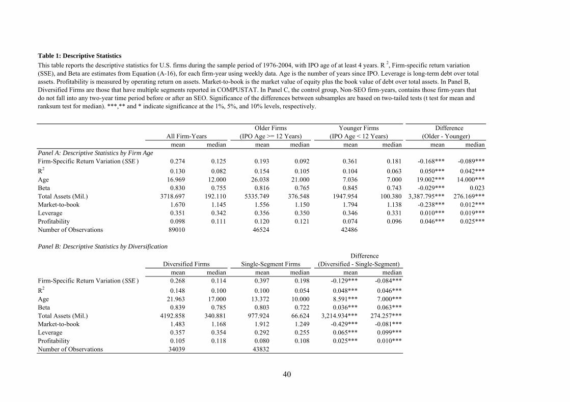
mean median mean median mean median mean medianPanel A: Descriptive Statistics by Firm AgeFirm-Specific Return Variation (SSE ) 0.274 0.125 0.193 0.092 0.361 0.181 -0.168*** -0.089***R2 0.130 0.082 0.154 0.105 0.104 0.063 0.050*** 0.042***Age 16.969 12.000 26.038 21.000 7.036 7.000 19.002*** 14.000***Beta 0.830 0.755 0.816 0.765 0.845 0.743 -0.029*** 0.023Total Assets (Mil.) 3718.697 192.110 5335.749 376.548 1947.954 100.380 3,387.795*** 276.169***Market-to-book 1.670 1.145 1.556 1.150 1.794 1.138 -0.238*** 0.012***Leverage 0.351 0.342 0.356 0.350 0.346 0.331 0.010*** 0.019***Profitability 0.098 0.111 0.120 0.121 0.074 0.096 0.046*** 0.025***Number of Observations 89010 46524 42486

Panel B: Descriptive Statistics by Diversification

mean median mean median mean medianFirm-Specific Return Variation (SSE ) 0.268 0.114 0.397 0.198 -0.129*** -0.084***R2 0.148 0.100 0.100 0.054 0.048*** 0.046***Age 21.963 17.000 13.372 10.000 8.591*** 7.000***Beta 0.839 0.785 0.803 0.722 0.036*** 0.063***Total Assets (Mil.) 4192.858 340.881 977.924 66.624 3,214.934*** 274.257***Market-to-book 1.483 1.168 1.912 1.249 -0.429*** -0.081***Leverage 0.357 0.354 0.292 0.255 0.065*** 0.099***Profitability 0.105 0.118 0.080 0.108 0.025*** 0.010***Number of Observations 34039 43832

All Firm-YearsOlder Firms

(IPO Age >= 12 Years)Younger Firms

(IPO Age < 12 Years) Difference

(Older - Younger)

Difference (Diversified - Single-Segment)Diversified Firms Single-Segment Firms

Table 1: Descriptive StatisticsThis table reports the descriptive statistics for U.S. firms during the sample period of 1976-2004, with IPO age of at least 4 years. R 2, Firm-specific return variation (SSE), and Beta are estimates from Equation (A-16), for each firm-year using weekly data. Age is the number of years since IPO. Leverage is long-term debt over total assets. Profitability is measured by operating return on assets. Market-to-book is the market value of equity plus the book value of debt over total assets. In Panel B, Diversified Firms are those that have multiple segments reported in COMPUSTAT. In Panel C, the control group, Non-SEO firm-years, contains those firm-years that do not fall into any two-year time period before or after an SEO. Significance of the differences between subsamples are based on two-tailed tests (t test for mean and ranksum test for median). ***,** and * indicate significance at the 1%, 5%, and 10% levels, respectively.

40

Table 1. Descriptive Statistics (Continued)

mean median mean median mean median mean median mean median mean medianFirm-Specific Return Variation (SSE ) 0.274 0.125 0.278 0.123 0.231 0.138 -0.046* 0.0145*** 0.235 0.139 -0.043 0.015***R2 0.130 0.082 0.127 0.078 0.156 0.119 0.029*** 0.041*** 0.175 0.139 0.048*** 0.061***Age 16.969 12.000 16.920 12.000 18.038 12.000 1.118*** 0.000*** 16.699 12.000 -0.221 0.000***Beta 0.830 0.755 0.802 0.731 1.054 0.955 0.251*** 0.224*** 1.146 1.076 0.343*** 0.345***Total Assets (Mil.) 3718.697 192.110 3799.463 177.195 2780 325.504 -1019.789** 148.309*** 3138.474 397.202 -660.989 220.007***Market-to-book 1.670 1.145 1.657 1.134 1.876 1.263 0.218*** 0.128*** 1.692 1.254 0.034 0.119***Leverage ratio 0.351 0.342 0.351 0.341 0.368 0.372 0.017*** 0.030*** 0.339 0.333 -0.011** -0.008**Profitability 0.098 0.111 0.098 0.110 0.099 0.120 0.001 0.009*** 0.082 0.110 -0.016*** -0.000***Number of Observations 89010 80633 4604 3773

0-2 Years Before SEO

1-2 Years After SEO

Panel C. Descriptive Statistics of the SEO sample vs. the Non-SEO sample

All Firm-YearsNon-SEO Firm-

Years Difference

(Before SEO - Non-SEO) Difference

(After SEO - Non-SEO)

41

Standard Market Model

Industry-Augmented

Market Model FF Three-

Factor ModelFF Three Factors plus Momentum

Standard Market Model

Industry-Augmented

Market Model FF Three-

Factor ModelFF Three Factors plus

Momentum (1) (2) (3) (4) (5) (6) (7) (8)

Panel A: Basic ModelLog(Age) -0.040*** -0.018** -0.026*** -0.029*** -0.044*** -0.023*** -0.023*** -0.025***

(0.005) (0.007) (0.006) (0.006) (0.005) (0.007) (0.007) (0.007) Market-to-book 0.003 0 0 0.002** -0.001 0 -0.001 0.001

(0.002) (0.001) (0.001) (0.001) (0.001) (0.001) (0.002) (0.001) Beta (Market factor) -0.089*** -0.091*** -0.030*** -0.020*** -0.107*** -0.084*** -0.028*** -0.017**

(0.012) (0.003) (0.011) (0.007) (0.005) (0.005) (0.011) (0.007) Beta (Industry return) -0.152*** -0.119***

(0.007) (0.008) Beta (High-minus-low factor) 0.024*** 0.021*** 0.025*** 0.021***

(0.003) (0.002) (0.002) (0.002) Beta (Small-minus-big factor) 0.001 -0.001 -0.002 -0.002

(0.004) (0.003) (0.004) (0.003) Beta (Momentum factor) 0.004 0.004

(0.003) (0.003) Log of total volatility 0.932*** 0.990*** 0.872*** 0.861*** 0.947*** 0.923*** 0.873*** 0.861***

(0.011) (0.008) (0.012) (0.008) (0.008) (0.008) (0.012) (0.009) Log(Assets) -0.030*** -0.036*** -0.048*** -0.053*** -0.021*** -0.037*** -0.044*** -0.050***

(0.004) (0.003) (0.003) (0.003) (0.002) (0.003) (0.003) (0.003) Profitability -0.018 -0.015 -0.013 -0.023*** -0.003 -0.003 -0.01 -0.022***

(0.013) (0.009) (0.011) (0.008) (0.009) (0.012) (0.013) (0.009) Leverage 0.051*** 0.055*** 0.067*** 0.074*** 0.051*** 0.070*** 0.073*** 0.079***

(0.007) (0.009) (0.007) (0.008) (0.007) (0.009) (0.008) (0.008) Idiosyncratic ROA movement 0.003*** 0.003*** 0.003*** 0.003***

(0.001) (0.001) (0.001) (0.001) Constant 13.142*** 3.944*** 3.668*** 3.642*** 13.188*** 3.804*** 3.657*** 3.624***

(0.035) (0.041) (0.045) (0.036) (0.030) (0.038) (0.047) (0.038) Observations 89010 88133 88979 88968 73156 73094 73146 73137Number of Firms 12015 11934 12011 12011 9806 9803 9804 9804R-squared 0.94 0.89 0.91 0.91 0.94 0.90 0.91 0.91

Controlling for ROA comovement

Table 2: Age and R2

This table estimates the effect of firm age on R2 as follows: R2and Beta are estimated from a market model (Equation A-16) in columns (1) and (5); from an industry-augmented market model in columns (2) and (6); and Fama-French (FF) three- factor and a four-factor model with momentum (Equations A-17 and A-18) in columns (3), (4), (7), and (8). Age is the number of years since the inclusion in CRSP. Size is the log of market value of assets. Leverage is long-term debt over total assets. Profitability is measured by operating return on assets. Market-to-book is the market value of equity plus book value of debt over total assets. Total volatility is the standard deviation of weekly return over one year. Diversification indicates whether the firm has multiple COMPUSTAT segments reported. Standard errors are clustered at the firm level and are in parenthesis. ***, ** and * indicate significance at the 1%, 5%, and 10% levels, respectively.

2, , , ,log(1 ) Age Firm Controls ,i t i t i t i t i tR α β γ η δ ε− = + + + + +

42

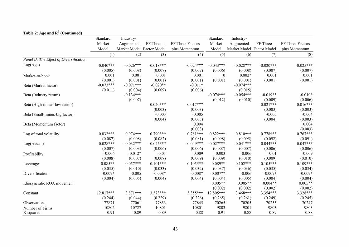
Table 2: Age and R2 (Continued)Standard Market Model

Industry-Augmented

Market Model FF Three-

Factor ModelFF Three Factors plus Momentum

Standard Market Model

Industry-Augmented

Market Model FF Three-

Factor ModelFF Three Factors plus Momentum

(1) (2) (3) (4) (5) (6) (7) (8)Panel B: The Effect of DiversificationLog(Age) -0.040*** -0.026*** -0.018*** -0.024*** -0.043*** -0.028*** -0.020*** -0.025***

(0.005) (0.008) (0.007) (0.007) (0.006) (0.008) (0.007) (0.007) Market-to-book 0.001 0.001 0.001 0.001 0 0.002* 0.001 0.001

(0.001) (0.001) (0.001) (0.001) (0.001) (0.001) (0.001) (0.001) Beta (Market factor) -0.073*** -0.071*** -0.020** -0.011* -0.074***

(0.011) (0.004) (0.009) (0.006) (0.015) Beta (Industry return) -0.134*** -0.074*** -0.054*** -0.019** -0.010*

(0.007) (0.012) (0.010) (0.009) (0.006) Beta (High-minus-low factor) 0.020*** 0.017*** 0.021*** 0.016***

(0.003) (0.003) (0.003) (0.003) Beta (Small-minus-big factor) -0.003 -0.005 -0.005 -0.004

(0.004) (0.003) (0.004) (0.003) Beta (Momentum factor) 0.004 0.004

(0.003) (0.003) Log of total volatility 0.832*** 0.974*** 0.790*** 0.781*** 0.822*** 0.810*** 0.778*** 0.767***

(0.087) (0.008) (0.082) (0.081) (0.098) (0.095) (0.092) (0.091) Log(Assets) -0.028*** -0.032*** -0.045*** -0.049*** -0.027*** -0.041*** -0.044*** -0.047***

(0.007) (0.003) (0.006) (0.006) (0.007) (0.007) (0.006) (0.006) Profitability -0.006 -0.012* -0.01 -0.009 -0.003 -0.006 -0.01 -0.009

(0.008) (0.007) (0.008) (0.009) (0.009) (0.010) (0.009) (0.010) Leverage 0.085** 0.057*** 0.101*** 0.105*** 0.089** 0.102*** 0.105*** 0.109***

(0.035) (0.010) (0.033) (0.032) (0.037) (0.036) (0.035) (0.034) Diversification -0.007* -0.005 -0.008* -0.008* -0.007** -0.006 -0.007* -0.007*

(0.004) (0.005) (0.004) (0.004) (0.004) (0.005) (0.004) (0.004) Idiosyncratic ROA movement 0.005** 0.005** 0.004** 0.005**

(0.002) (0.002) (0.002) (0.002) Constant 12.817*** 3.871*** 3.373*** 3.355*** 12.805*** 3.468*** 3.354*** 3.328***

(0.244) (0.044) (0.229) (0.226) (0.265) (0.261) (0.249) (0.245) Observations 77871 77061 77853 77845 70265 70205 70253 70247Number of Firms 10802 10727 10801 10801 9803 9801 9803 9803R-squared 0.91 0.89 0.89 0.88 0.91 0.88 0.89 0.88

43

Industry augmented

market modelFF Three-Factor

ModelFF Three Factors plus Momentum

(1) (2) (3) (4) (5)1-2 years prior to SEO 0.006 0.011** 0.012*** 0.009**

(0.004) (0.005) (0.004) (0.005) Year of SEO 0.002 0.003 -0.013* -0.007 -0.005

(0.004) (0.005) (0.008) (0.005) (0.006) 1-2 years subsequent to SEO -0.011*** -0.010*** -0.012** -0.012*** -0.016***

(0.004) (0.004) (0.005) (0.004) (0.004) Beta (Market factor) -0.089*** -0.089*** -0.091*** -0.030*** -0.020***

(0.012) (0.012) (0.003) (0.011) (0.007) Beta (High-minus-low factor) 0.024*** 0.021***

(0.003) (0.002) Beta (Small-minus-big factor) 0.001 -0.001

(0.004) (0.003) Beta (Momentum factor) 0.004

(0.003) Beta (Industry return) -0.152***

(0.007) Log of total volatility 0.932*** 0.932*** 0.991*** 0.873*** 0.862***

(0.010) (0.010) (0.008) (0.012) (0.008) Market-to-book 0.002 0.002 0 0 0.002**

(0.002) (0.002) (0.001) (0.001) (0.001) Log(Age) -0.040*** -0.040*** -0.018*** -0.027*** -0.030***

(0.005) (0.005) (0.007) (0.006) (0.006) Log(Assets) -0.029*** -0.029*** -0.035*** -0.047*** -0.052***

(0.004) (0.004) (0.003) (0.003) (0.003) Profitability -0.019 -0.019 -0.015 -0.013 -0.023***

(0.013) (0.013) (0.009) (0.011) (0.008) Leverage 0.050*** 0.050*** 0.053*** 0.066*** 0.073***

(0.007) (0.007) (0.009) (0.008) (0.008) Constant 13.141*** 13.141*** 3.942*** 3.666*** 3.641***

(0.035) (0.035) (0.042) (0.045) (0.036) Observations 89010 89010 88133 88979 88968Number of permno 12015 12015 11934 12011 12011R-squared 0.94 0.94 0.89 0.91 0.91

Standard Market Model

Table 3. The Dynamic Response of R2 to SEOsThis table reports the dynamics of R2 in response to SEOs from the model below:

R2 and Beta are estimated from a market model (Equation A-16) in columns (1) and (2); from an industry-augmented market model in column (3); from Fama and French (FF) three-factor and a four- factor model with momentum (Equations A-17 and A-18) in columns (4) and (5). Age is the number of years since the inclusion in CRSP. Size is the log of market assets. Leverage is long-term debt over total assets. Profitability is measured by the return on assets. Market-to-book is the market value of equity plus book value of debt over total assets. Total Volatility is the standard deviation of weekly return over a year. Standard error are clustered at the firm level and are in the parenthesis. ***, ** and * indicate significance at 1%, 5%, and 10% levels, respectively.

2, , i,t ,log(1 ) (SEO has occured k periods earlier) Firm Controlsi t k i t i t i t

kR α β γ η δ ε− = + + + + +∑

44

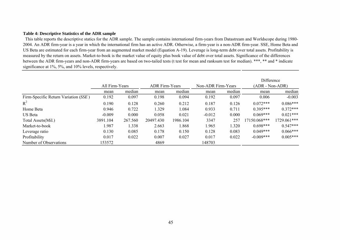
mean median mean median mean median mean medianFirm-Specific Return Variation (SSE ) 0.192 0.097 0.198 0.094 0.192 0.097 0.006 -0.003R2 0.190 0.128 0.260 0.212 0.187 0.126 0.072*** 0.086***Home Beta 0.946 0.722 1.329 1.084 0.933 0.711 0.395*** 0.372***US Beta -0.009 0.000 0.058 0.021 -0.012 0.000 0.069*** 0.021***Total Assets(Mil.) 3891.104 267.560 20497.430 1986.104 3347 257 17150.068*** 1729.061***Market-to-book 1.987 1.338 2.663 1.868 1.965 1.320 0.698*** 0.547***Leverage ratio 0.130 0.085 0.178 0.150 0.128 0.083 0.049*** 0.066***Profitability 0.017 0.022 0.007 0.027 0.017 0.022 -0.009*** 0.005***Number of Observations 153572 4869 148703

Difference (ADR - Non-ADR)All Firm-Years ADR Firm-Years Non-ADR Firm-Years

Table 4: Descriptive Statistics of the ADR sample This table reports the descriptive statics for the ADR sample. The sample contains international firm-years from Datastream and Worldscope during 1980-2004. An ADR firm-year is a year in which the international firm has an active ADR. Otherwise, a firm-year is a non-ADR firm-year. SSE, Home Beta and US Beta are estimated for each firm-year from an augmented market model (Equation A-19). Leverage is long-term debt over total assets. Profitability is measured by the return on assets. Market-to-book is the market value of equity plus book value of debt over total assets. Significance of the differences between the ADR firm-years and non-ADR firm-years are based on two-tailed tests (t test for mean and ranksum test for median). ***, ** and * indicate significance at 1%, 5%, and 10% levels, respectively.

45

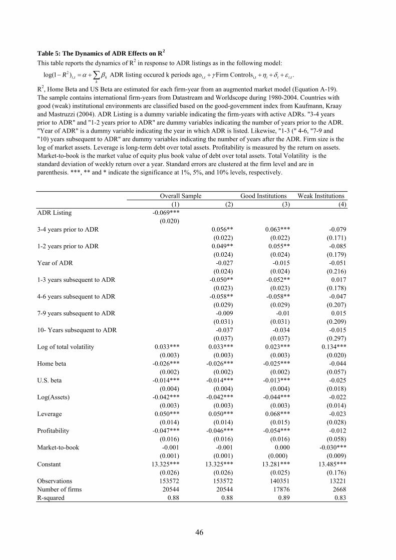
Good Institutions Weak Institutions(1) (2) (3) (4)

ADR Listing -0.069***(0.020)

3-4 years prior to ADR 0.056** 0.063*** -0.079(0.022) (0.022) (0.171)

1-2 years prior to ADR 0.049** 0.055** -0.085(0.024) (0.024) (0.179)

Year of ADR -0.027 -0.015 -0.051(0.024) (0.024) (0.216)

1-3 years subsequent to ADR -0.050** -0.052** 0.017(0.023) (0.023) (0.178)

4-6 years subsequent to ADR -0.058** -0.058** -0.047(0.029) (0.029) (0.207)

7-9 years subsequent to ADR -0.009 -0.01 0.015(0.031) (0.031) (0.209)

10- Years subsequent to ADR -0.037 -0.034 -0.015(0.037) (0.037) (0.297)

Log of total volatility 0.033*** 0.033*** 0.023*** 0.134***(0.003) (0.003) (0.003) (0.020)

Home beta -0.026*** -0.026*** -0.025*** -0.044(0.002) (0.002) (0.002) (0.057)

U.S. beta -0.014*** -0.014*** -0.013*** -0.025(0.004) (0.004) (0.004) (0.018)

Log(Assets) -0.042*** -0.042*** -0.044*** -0.022(0.003) (0.003) (0.003) (0.014)

Leverage 0.050*** 0.050*** 0.068*** -0.023(0.014) (0.014) (0.015) (0.028)

Profitability -0.047*** -0.046*** -0.054*** -0.012(0.016) (0.016) (0.016) (0.058)

Market-to-book -0.001 -0.001 0.000 -0.030***(0.001) (0.001) (0.000) (0.009)

Constant 13.325*** 13.325*** 13.281*** 13.485***(0.026) (0.026) (0.025) (0.176)

Observations 153572 153572 140351 13221Number of firms 20544 20544 17876 2668R-squared 0.88 0.88 0.89 0.83

Overall Sample

Table 5: The Dynamics of ADR Effects on R2

This table reports the dynamics of R2 in response to ADR listings as in the following model:

R2, Home Beta and US Beta are estimated for each firm-year from an augmented market model (Equation A-19). The sample contains international firm-years from Datastream and Worldscope during 1980-2004. Countries with good (weak) institutional environments are classified based on the good-government index from Kaufmann, Kraay and Mastruzzi (2004). ADR Listing is a dummy variable indicating the firm-years with active ADRs. "3-4 years prior to ADR" and "1-2 years prior to ADR" are dummy variables indicating the number of years prior to the ADR. "Year of ADR" is a dummy variable indicating the year in which ADR is listed. Likewise, "1-3 (" 4-6, "7-9 and "10) years subsequent to ADR" are dummy variables indicating the number of years after the ADR. Firm size is the log of market assets. Leverage is long-term debt over total assets. Profitability is measured by the return on assets. Market-to-book is the market value of equity plus book value of debt over total assets. Total Volatility is the standard deviation of weekly return over a year. Standard errors are clustered at the firm level and are in parenthesis. ***, ** and * indicate the significance at 1%, 5%, and 10% levels, respectively.

2, , i,t ,log(1 ) ADR listing occured k periods ago Firm Controls .i t k i t i t i t

kR α β γ η δ ε− = + + + + +∑

46