Dr. MCR HRDIAP

Training Program on

Spreadsheet Applications

Dr. MCRHRD Institute of Andhra Pradesh

Dr. MCR HRDIAP

Trademark Acknowledgement

All Products are registered trademarks of their respective organization. All software used is

for training purpose only.

This book has been specially designed for imparting ICT Education to Government officials

working in various departments in the Government of Andhra Pradesh.

Dr. MCRHRD IAP, Hyderabad designed and developed this courseware in English on

“Computer Fundamentals & Office Applications”. Copyright © Dr. MCRHRD IAP Hyderabad

2013. All Rights reserved.

No part of this publication may be reproduced, stored in retrieval, system, or transmitted in

any form, or by any means, electronic, mechanical, photocopying, recording or otherwise,

without the prior written permission of the publisher.

Dr. MCR HRDIAP

CONTENT

Introduction 1

1.1 Spreadsheets 1

1.2 Interface Elements 2

1.3 Data Entry in Excel 5

1.4 File Tab 9

1.5 Home Tab 12

1.6 Insert Tab 14

1.7 Page Layout Tab 15

1.8 Formulas Tab 15

1.9 Data Tab 18

1.10 Review Tab 19

1.11 View Tab 19

Functions in Excel 22

2.1 Enter Functions 22

2.2 Text Functions 23

2.3 Date Functions 23

2.4 PMT Function 23

2.5 Logical Function If 23

2.6 VLookUp 24

2.7 Formula Referencing in Excel 25

More Options on Data 27

3.1 Deleting options 27

3.2 Find and Replace 27

3.3 Conditional Formatting 27

3.4 Data Validation 28

3.5 Sort 29

3.6 Filter 29

3.7 Insert Subtotals in Excel 2010 Worksheets 30

3.8 Naming a Cell Range 30

3.9 Freeze Panes 32

3.10 Paste Special 34

Charts and Pivot Table 36

4.1 Charts 36

4.2 Pivot Table 38

Dr. MCR HRDIAP

What – If- Analysis and Macros 41

5.1 Scenario Manager 41

5.2 Goal Seek 43

5.3 Macros 44

Printing in Excel 47

6.1 Printing 47

6.2 Change Page Orientation 50

6.3 Print Titles 52

6.4 Insert a Break 54

Dr. MCR HRDIAP

1

INTRODUCTION

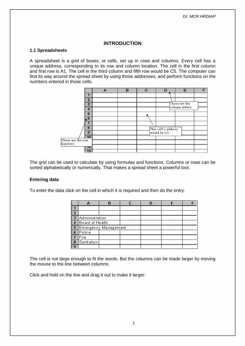
1.1 Spreadsheets

A spreadsheet is a grid of boxes, or cells, set up in rows and columns. Every cell has a unique address, corresponding to its row and column location. The cell in the first column and first row is A1. The cell in the third column and fifth row would be C5. The computer can find its way around the spread sheet by using those addresses, and perform functions on the numbers entered in those cells.

The grid can be used to calculate by using formulas and functions. Columns or rows can be sorted alphabetically or numerically. That makes a spread sheet a powerful tool.

Entering data

To enter the data click on the cell in which it is required and then do the entry.

The cell is not large enough to fit the words. But the columns can be made larger by moving the mouse to the line between columns.

Click and hold on the line and drag it out to make it larger:

Dr. MCR HRDIAP

2

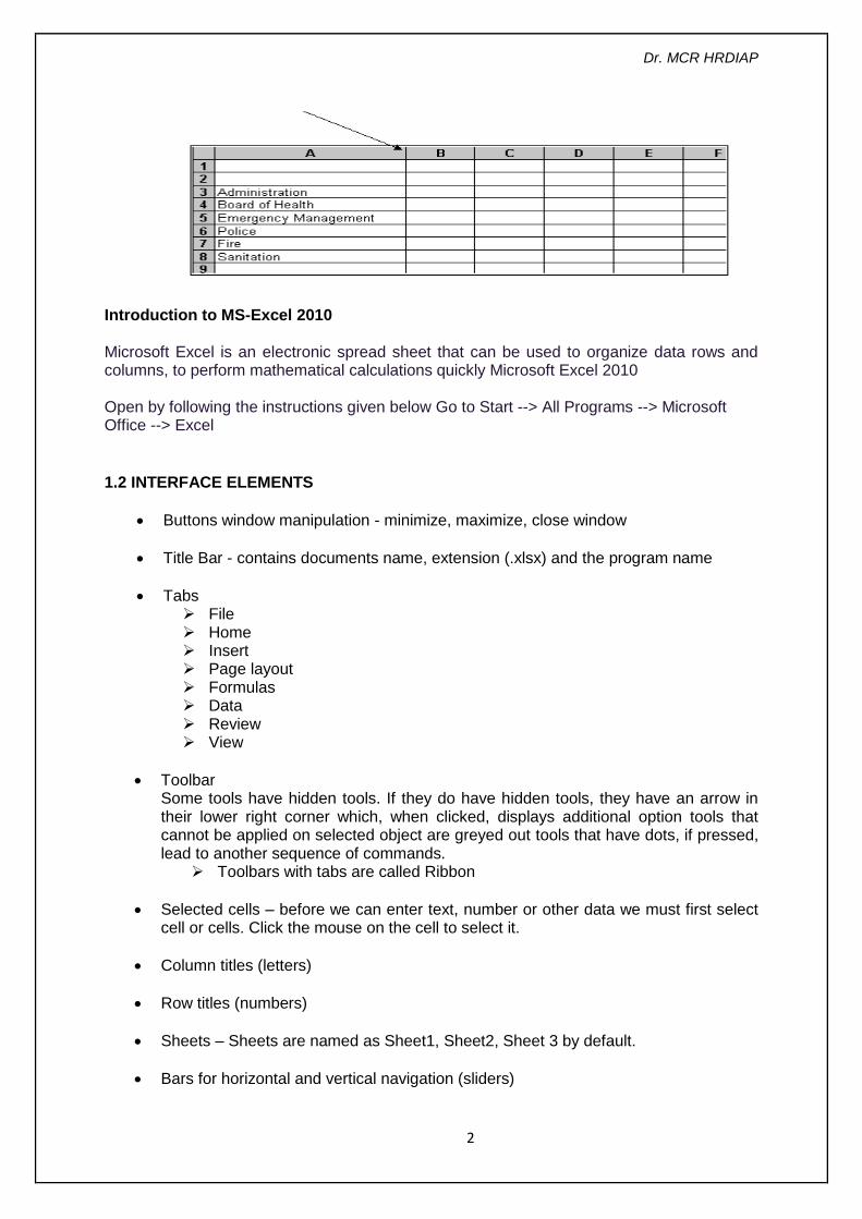
Introduction to MS-Excel 2010

Microsoft Excel is an electronic spread sheet that can be used to organize data rows and columns, to perform mathematical calculations quickly Microsoft Excel 2010

Open by following the instructions given below Go to Start --> All Programs --> Microsoft Office --> Excel

1.2 INTERFACE ELEMENTS

Buttons window manipulation - minimize, maximize, close window

Title Bar - contains documents name, extension (.xlsx) and the program name

Tabs File Home Insert Page layout Formulas Data Review View

Toolbar Some tools have hidden tools. If they do have hidden tools, they have an arrow in their lower right corner which, when clicked, displays additional option tools that cannot be applied on selected object are greyed out tools that have dots, if pressed, lead to another sequence of commands.

Toolbars with tabs are called Ribbon

Selected cells – before we can enter text, number or other data we must first select cell or cells. Click the mouse on the cell to select it.

Column titles (letters)

Row titles (numbers)

Sheets – Sheets are named as Sheet1, Sheet2, Sheet 3 by default.

Bars for horizontal and vertical navigation (sliders)

Dr. MCR HRDIAP

3

Status bar - displays information about some special functions of Microsoft Excel

Bar for formulas

Spread sheet: File in MS Excel, consisting of worksheets (3 by default)

Worksheet: consists of a large number of columns and rows that form a table Cell - the basic element in Excel, data entry (text, number, formula) Cell address: the column letter and row number, e.g. A1, C7, F25 Selecting cells - press left mouse button on the cell in order to select it

The Title Bar

On the Title bar, Microsoft Excel displays the name of the workbook, which is currently in use.

The Ribbon

In Microsoft Excel 2010, we use the Ribbon to issue commands.

The Ribbon is located near the top of the Excel window.

At the top of the Ribbon are several tabs;

Clicking a tab displays several related command groups.

Within each group are related command buttons.

Buttons are clicked to issue commands or to access menus and dialog boxes.

A dialog box launcher is found in the bottom-right corner of a group.

Click the dialog box launcher, a dialog box makes additional commands available.

Dr. MCR HRDIAP

4

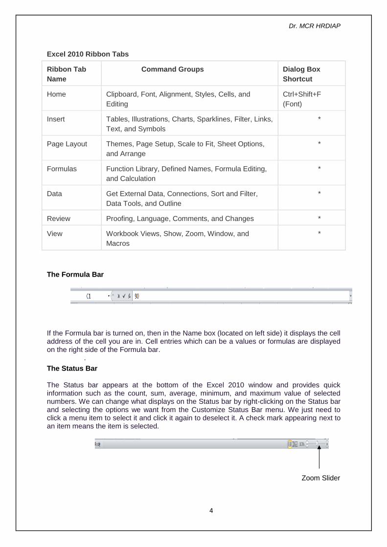
Excel 2010 Ribbon Tabs

Ribbon Tab

Name

Command Groups Dialog Box

Shortcut

Home Clipboard, Font, Alignment, Styles, Cells, and

Editing

Ctrl+Shift+F

(Font)

Insert Tables, Illustrations, Charts, Sparklines, Filter, Links,

Text, and Symbols

*

Page Layout Themes, Page Setup, Scale to Fit, Sheet Options,

and Arrange

*

Formulas Function Library, Defined Names, Formula Editing,

and Calculation

*

Data Get External Data, Connections, Sort and Filter,

Data Tools, and Outline

*

Review Proofing, Language, Comments, and Changes *

View Workbook Views, Show, Zoom, Window, and

Macros

*

The Formula Bar

If the Formula bar is turned on, then in the Name box (located on left side) it displays the cell address of the cell you are in. Cell entries which can be a values or formulas are displayed on the right side of the Formula bar.

.

The Status Bar

The Status bar appears at the bottom of the Excel 2010 window and provides quick information such as the count, sum, average, minimum, and maximum value of selected numbers. We can change what displays on the Status bar by right-clicking on the Status bar and selecting the options we want from the Customize Status Bar menu. We just need to click a menu item to select it and click it again to deselect it. A check mark appearing next to an item means the item is selected.

Zoom Slider

Dr. MCR HRDIAP

5

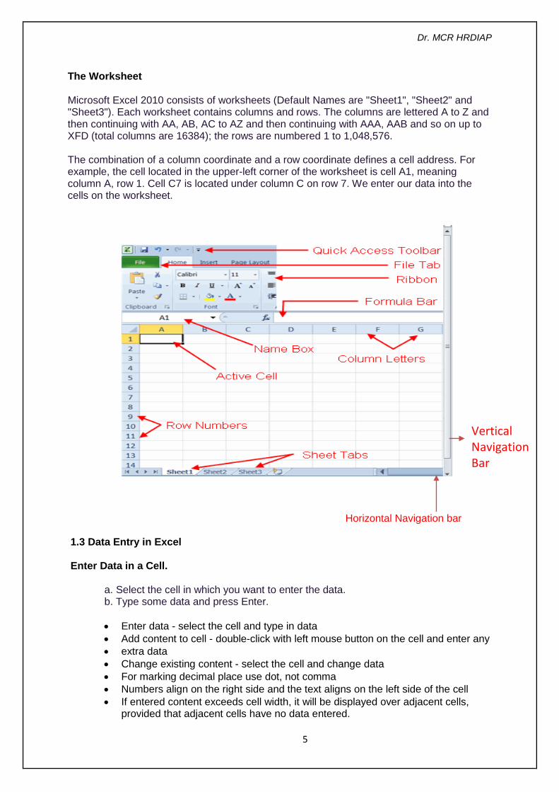
The Worksheet

Microsoft Excel 2010 consists of worksheets (Default Names are "Sheet1", "Sheet2" and "Sheet3"). Each worksheet contains columns and rows. The columns are lettered A to Z and then continuing with AA, AB, AC to AZ and then continuing with AAA, AAB and so on up to XFD (total columns are 16384); the rows are numbered 1 to 1,048,576. The combination of a column coordinate and a row coordinate defines a cell address. For example, the cell located in the upper-left corner of the worksheet is cell A1, meaning column A, row 1. Cell C7 is located under column C on row 7. We enter our data into the cells on the worksheet.

Horizontal Navigation bar

1.3 Data Entry in Excel

Enter Data in a Cell.

a. Select the cell in which you want to enter the data. b. Type some data and press Enter.

Enter data - select the cell and type in data

Add content to cell - double-click with left mouse button on the cell and enter any

extra data

Change existing content - select the cell and change data

For marking decimal place use dot, not comma

Numbers align on the right side and the text aligns on the left side of the cell

If entered content exceeds cell width, it will be displayed over adjacent cells, provided that adjacent cells have no data entered.

Vertical Navigation Bar

Dr. MCR HRDIAP

6

To move to another cell: you can use TAB key, keys with arrow on the keyboard, or left mouse button

Select a range of cells:

Select the first cell in the range, press and hold left mouse button, move the mouse to the last cell and release left button.

Or

Select the first cell in the range, press and hold the Shift key, select the last cell in range and release the Shift key

Select a row or column: press the mouse button on the row number or column letter

Select several adjacent rows: press the left mouse button on the row number, press and hold left mouse button, move the mouse to the last row and release the left button (or use Shift key, while Shift key is pressed select first then last row then release the Shift key)

Select several nonadjacent cells, rows and columns: press left mouse button on the row number in order to select it, press and hold Ctrl key, select other rows and then release Ctrl key

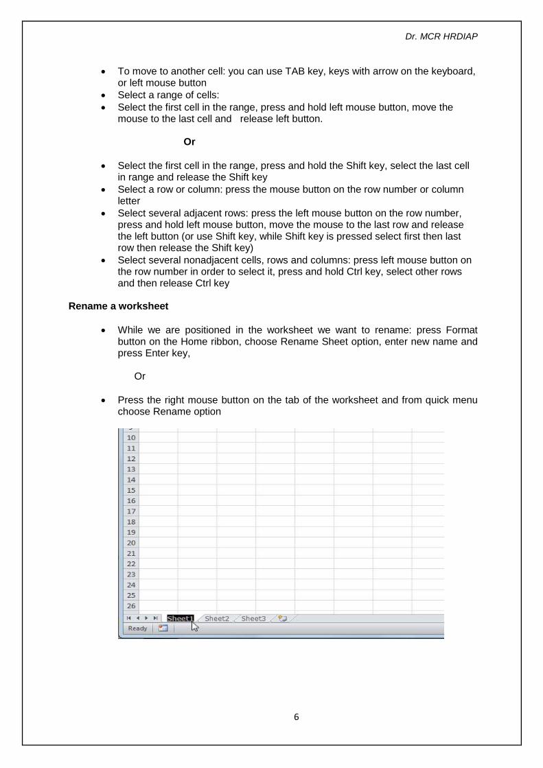
Rename a worksheet

While we are positioned in the worksheet we want to rename: press Format button on the Home ribbon, choose Rename Sheet option, enter new name and press Enter key,

Or

Press the right mouse button on the tab of the worksheet and from quick menu choose Rename option

Dr. MCR HRDIAP

7

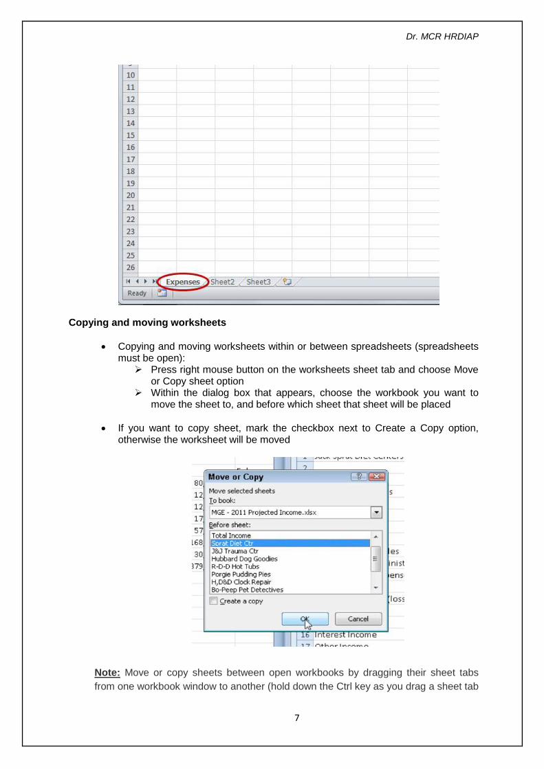
Copying and moving worksheets

Copying and moving worksheets within or between spreadsheets (spreadsheets must be open):

Press right mouse button on the worksheets sheet tab and choose Move or Copy sheet option

Within the dialog box that appears, choose the workbook you want to move the sheet to, and before which sheet that sheet will be placed

If you want to copy sheet, mark the checkbox next to Create a Copy option, otherwise the worksheet will be moved

Note: Move or copy sheets between open workbooks by dragging their sheet tabs

from one workbook window to another (hold down the Ctrl key as you drag a sheet tab

Dr. MCR HRDIAP

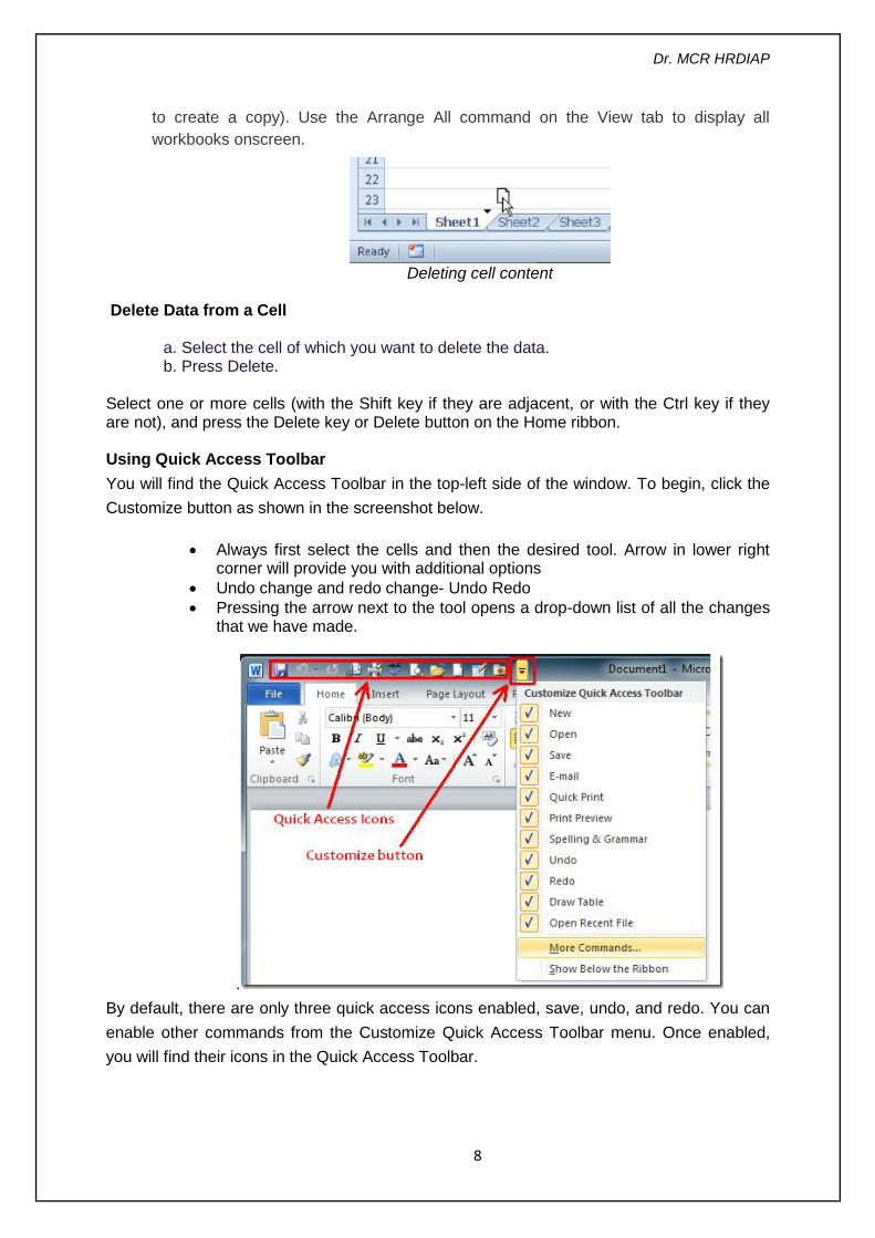
8

to create a copy). Use the Arrange All command on the View tab to display all

workbooks onscreen.

Deleting cell content

Delete Data from a Cell

a. Select the cell of which you want to delete the data. b. Press Delete.

Select one or more cells (with the Shift key if they are adjacent, or with the Ctrl key if they are not), and press the Delete key or Delete button on the Home ribbon.

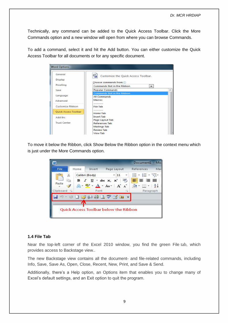
Using Quick Access Toolbar

You will find the Quick Access Toolbar in the top-left side of the window. To begin, click the

Customize button as shown in the screenshot below.

Always first select the cells and then the desired tool. Arrow in lower right corner will provide you with additional options

Undo change and redo change- Undo Redo

Pressing the arrow next to the tool opens a drop-down list of all the changes that we have made.

.

By default, there are only three quick access icons enabled, save, undo, and redo. You can

enable other commands from the Customize Quick Access Toolbar menu. Once enabled,

you will find their icons in the Quick Access Toolbar.

Dr. MCR HRDIAP

9

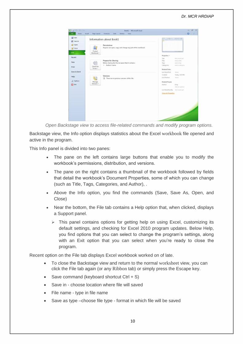
Technically, any command can be added to the Quick Access Toolbar. Click the More

Commands option and a new window will open from where you can browse Commands.

To add a command, select it and hit the Add button. You can either customize the Quick

Access Toolbar for all documents or for any specific document.

To move it below the Ribbon, click Show Below the Ribbon option in the context menu which

is just under the More Commands option.

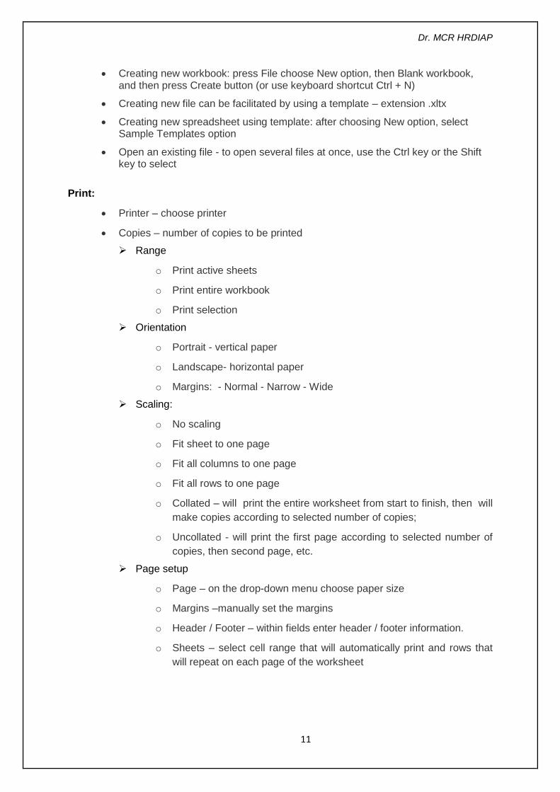
1.4 File Tab

Near the top-left corner of the Excel 2010 window, you find the green File tab, which

provides access to Backstage view..

The new Backstage view contains all the document- and file-related commands, including

Info, Save, Save As, Open, Close, Recent, New, Print, and Save & Send.

Additionally, there’s a Help option, an Options item that enables you to change many of

Excel’s default settings, and an Exit option to quit the program.

Dr. MCR HRDIAP

10

Open Backstage view to access file-related commands and modify program options.

Backstage view, the Info option displays statistics about the Excel workbook file opened and

active in the program.

This Info panel is divided into two panes:

The pane on the left contains large buttons that enable you to modify the

workbook’s permissions, distribution, and versions.

The pane on the right contains a thumbnail of the workbook followed by fields

that detail the workbook’s Document Properties, some of which you can change

(such as Title, Tags, Categories, and Author), .

Above the Info option, you find the commands (Save, Save As, Open, and

Close)

Near the bottom, the File tab contains a Help option that, when clicked, displays

a Support panel.

This panel contains options for getting help on using Excel, customizing its

default settings, and checking for Excel 2010 program updates. Below Help,

you find options that you can select to change the program’s settings, along

with an Exit option that you can select when you’re ready to close the

program.

Recent option on the File tab displays Excel workbook worked on of late.

To close the Backstage view and return to the normal worksheet view, you can

click the File tab again (or any Ribbon tab) or simply press the Escape key.

Save command (keyboard shortcut Ctrl + S)

Save in - choose location where file will saved

File name - type in file name

Save as type –choose file type - format in which file will be saved

Dr. MCR HRDIAP

11

Creating new workbook: press File choose New option, then Blank workbook, and then press Create button (or use keyboard shortcut Ctrl + N)

Creating new file can be facilitated by using a template – extension .xltx

Creating new spreadsheet using template: after choosing New option, select Sample Templates option

Open an existing file - to open several files at once, use the Ctrl key or the Shift key to select

Print:

Printer – choose printer

Copies – number of copies to be printed

Range

o Print active sheets

o Print entire workbook

o Print selection

Orientation

o Portrait - vertical paper

o Landscape- horizontal paper

o Margins: - Normal - Narrow - Wide

Scaling:

o No scaling

o Fit sheet to one page

o Fit all columns to one page

o Fit all rows to one page

o Collated – will print the entire worksheet from start to finish, then will

make copies according to selected number of copies;

o Uncollated - will print the first page according to selected number of

copies, then second page, etc.

Page setup

o Page – on the drop-down menu choose paper size

o Margins –manually set the margins

o Header / Footer – within fields enter header / footer information.

o Sheets – select cell range that will automatically print and rows that

will repeat on each page of the worksheet

Dr. MCR HRDIAP

12

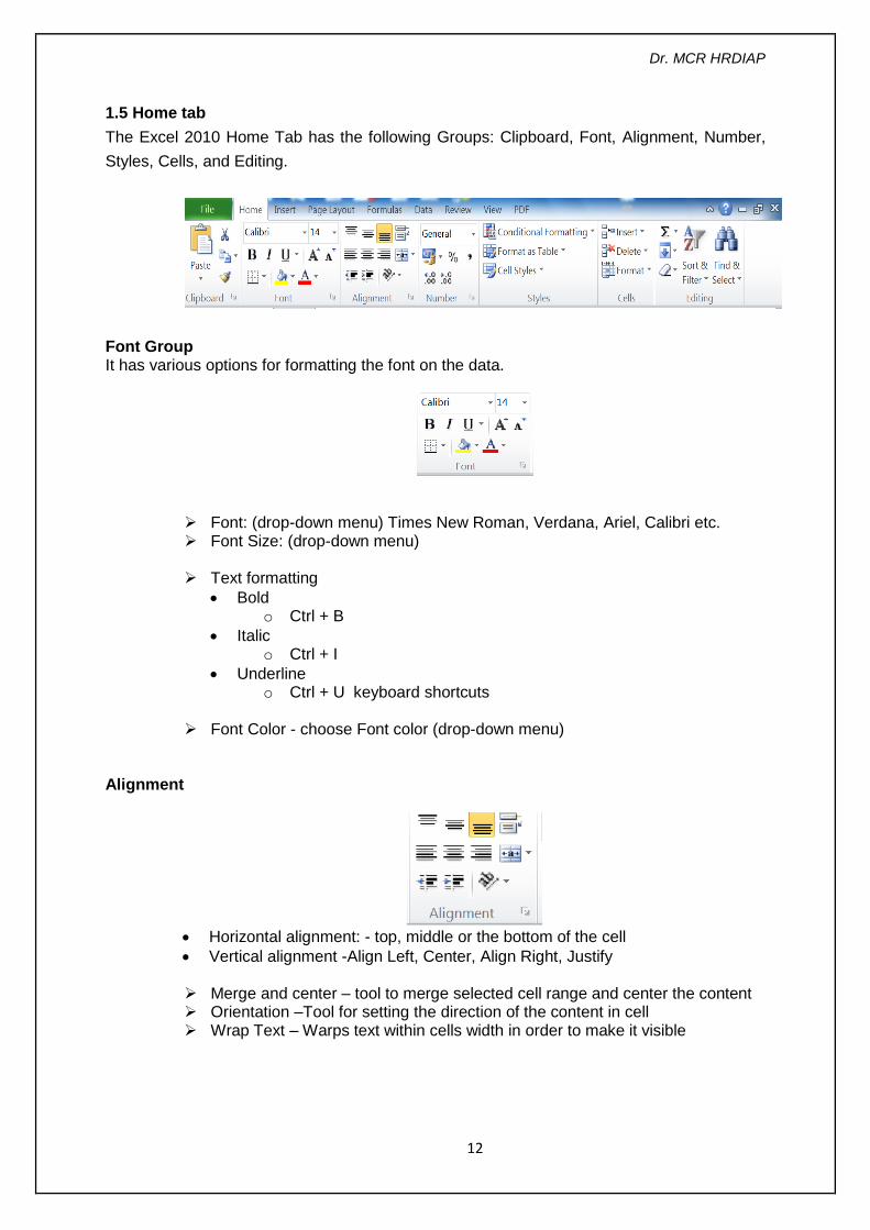
1.5 Home tab

The Excel 2010 Home Tab has the following Groups: Clipboard, Font, Alignment, Number,

Styles, Cells, and Editing.

Font Group It has various options for formatting the font on the data.

Font: (drop-down menu) Times New Roman, Verdana, Ariel, Calibri etc. Font Size: (drop-down menu) Text formatting

Bold o Ctrl + B

Italic o Ctrl + I

Underline o Ctrl + U keyboard shortcuts

Font Color - choose Font color (drop-down menu)

Alignment

Horizontal alignment: - top, middle or the bottom of the cell

Vertical alignment -Align Left, Center, Align Right, Justify

Merge and center – tool to merge selected cell range and center the content Orientation –Tool for setting the direction of the content in cell Wrap Text – Warps text within cells width in order to make it visible

Dr. MCR HRDIAP

13

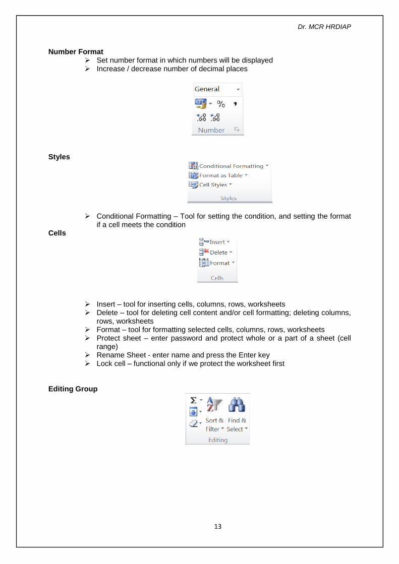
Number Format Set number format in which numbers will be displayed Increase / decrease number of decimal places

Styles

Conditional Formatting – Tool for setting the condition, and setting the format if a cell meets the condition

Cells

Insert – tool for inserting cells, columns, rows, worksheets Delete – tool for deleting cell content and/or cell formatting; deleting columns,

rows, worksheets Format – tool for formatting selected cells, columns, rows, worksheets Protect sheet – enter password and protect whole or a part of a sheet (cell

range) Rename Sheet - enter name and press the Enter key Lock cell – functional only if we protect the worksheet first

Editing Group

Dr. MCR HRDIAP

14

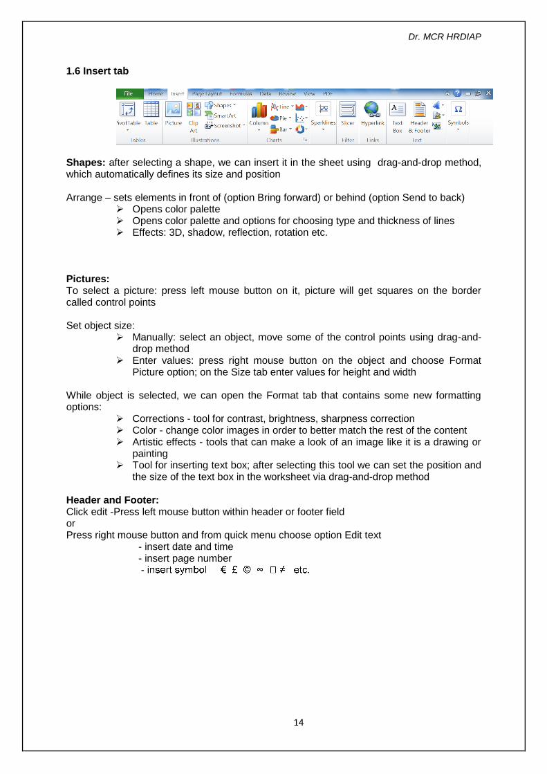
1.6 Insert tab

Shapes: after selecting a shape, we can insert it in the sheet using drag-and-drop method, which automatically defines its size and position

Arrange – sets elements in front of (option Bring forward) or behind (option Send to back)

Opens color palette Opens color palette and options for choosing type and thickness of lines Effects: 3D, shadow, reflection, rotation etc.

Pictures: To select a picture: press left mouse button on it, picture will get squares on the border called control points

Set object size:

Manually: select an object, move some of the control points using drag-and-drop method

Enter values: press right mouse button on the object and choose Format Picture option; on the Size tab enter values for height and width

While object is selected, we can open the Format tab that contains some new formatting options:

Corrections - tool for contrast, brightness, sharpness correction Color - change color images in order to better match the rest of the content Artistic effects - tools that can make a look of an image like it is a drawing or

painting Tool for inserting text box; after selecting this tool we can set the position and

the size of the text box in the worksheet via drag-and-drop method

Header and Footer: Click edit -Press left mouse button within header or footer field or Press right mouse button and from quick menu choose option Edit text

- insert date and time - insert page number

- i

Dr. MCR HRDIAP

15

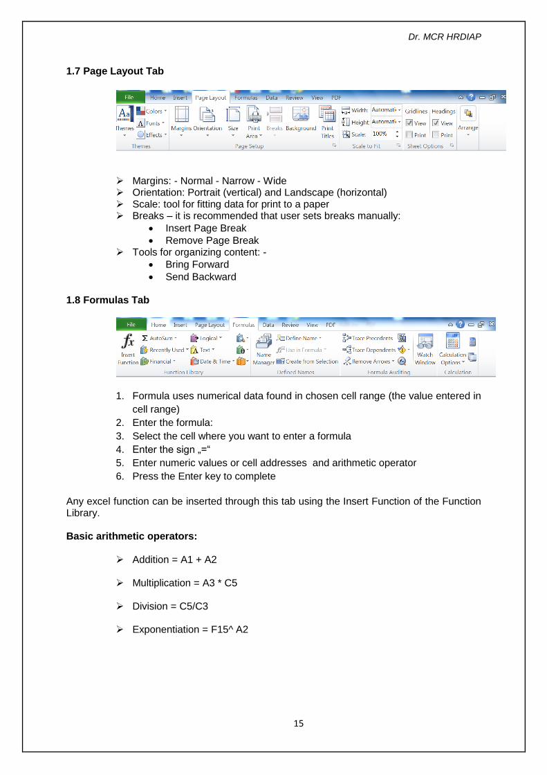
1.7 Page Layout Tab

Margins: - Normal - Narrow - Wide Orientation: Portrait (vertical) and Landscape (horizontal) Scale: tool for fitting data for print to a paper Breaks – it is recommended that user sets breaks manually:

Insert Page Break

Remove Page Break Tools for organizing content: -

Bring Forward

Send Backward 1.8 Formulas Tab

1. Formula uses numerical data found in chosen cell range (the value entered in

cell range)

2. Enter the formula:

3. Select the cell where you want to enter a formula

4. Enter the sign „=“

5. Enter numeric values or cell addresses and arithmetic operator

6. Press the Enter key to complete

Any excel function can be inserted through this tab using the Insert Function of the Function Library.

Basic arithmetic operators:

Addition = A1 + A2 Multiplication = A3 * C5 Division = C5/C3 Exponentiation = F15^ A2

Dr. MCR HRDIAP

16

Calculation order

Microsoft Excel follows the mathematical order of calculation operations.

Formulas can be seen in the formula bar when cell that contains formula is selected

or if we position cursor with double click in the cell that contains formula (this way formula will be visible in cell to, and can be edited in a cell to).

Cell that contains formula and cursor is not positioned in that particular cell, will

display formula result.

Function Library

There are hundreds of functions in Excel, but only some will be useful for the kind of

data we work with.

To explore functions is in the Function Library on the Formulas tab. Here you may

search and select Excel functions based on categories such

as Financial, Logical, Text, Date & Time, and more.

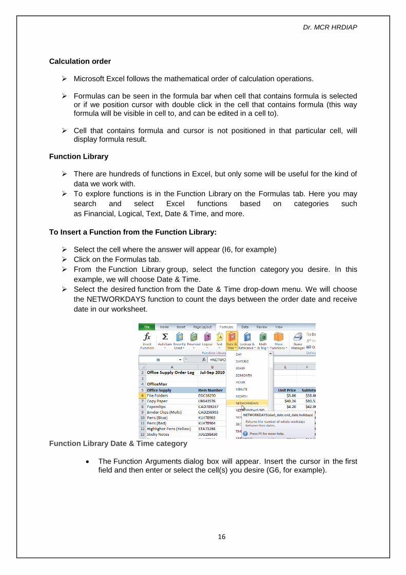
To Insert a Function from the Function Library:

Select the cell where the answer will appear (I6, for example)

Click on the Formulas tab.

From the Function Library group, select the function category you desire. In this

example, we will choose Date & Time.

Select the desired function from the Date & Time drop-down menu. We will choose

the NETWORKDAYS function to count the days between the order date and receive

date in our worksheet.

Function Library Date & Time category

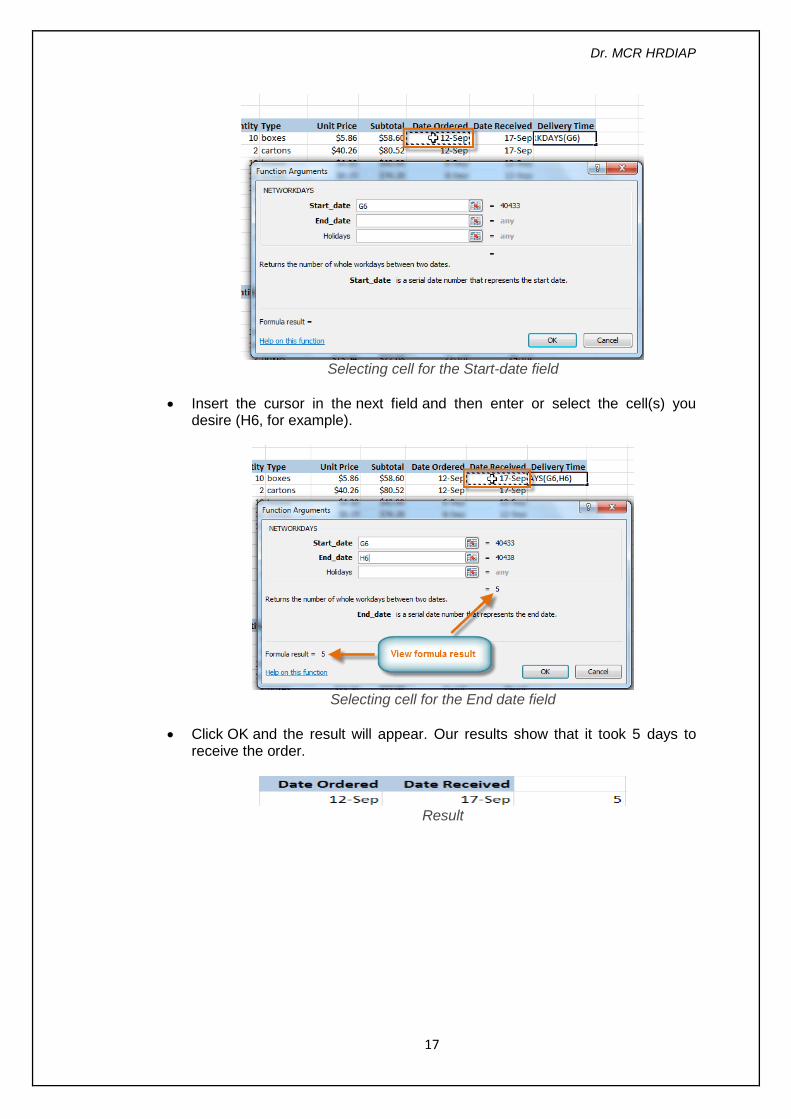
The Function Arguments dialog box will appear. Insert the cursor in the first field and then enter or select the cell(s) you desire (G6, for example).

Dr. MCR HRDIAP

17

Selecting cell for the Start-date field

Insert the cursor in the next field and then enter or select the cell(s) you desire (H6, for example).

Selecting cell for the End date field

Click OK and the result will appear. Our results show that it took 5 days to receive the order.

Result

Dr. MCR HRDIAP

18

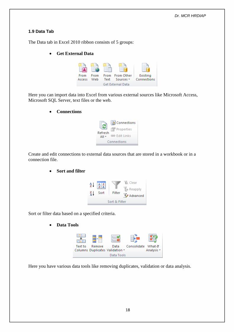
1.9 Data Tab

The Data tab in Excel 2010 ribbon consists of 5 groups:

Get External Data

Here you can import data into Excel from various external sources like Microsoft Access,

Microsoft SQL Server, text files or the web.

Connections

Create and edit connections to external data sources that are stored in a workbook or in a

connection file.

Sort and filter

Sort or filter data based on a specified criteria.

Data Tools

Here you have various data tools like removing duplicates, validation or data analysis.

Dr. MCR HRDIAP

19

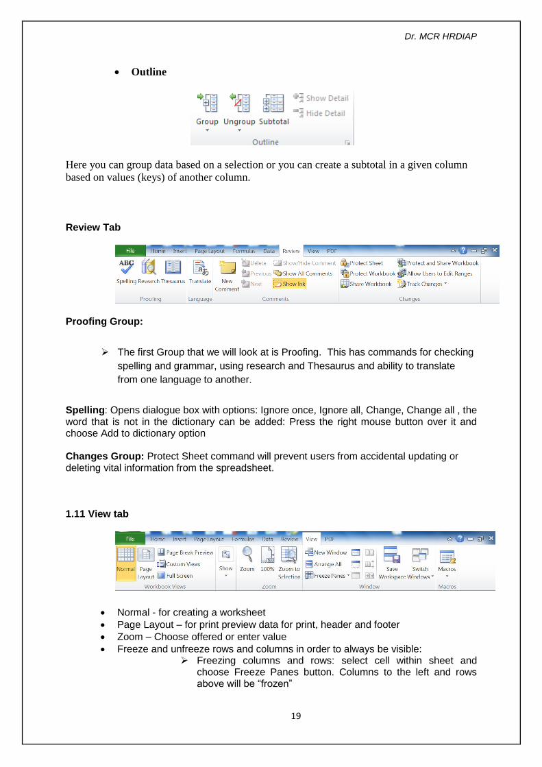
Outline

Here you can group data based on a selection or you can create a subtotal in a given column

based on values (keys) of another column.

Review Tab

Proofing Group:

The first Group that we will look at is Proofing. This has commands for checking

spelling and grammar, using research and Thesaurus and ability to translate

from one language to another.

Spelling: Opens dialogue box with options: Ignore once, Ignore all, Change, Change all , the word that is not in the dictionary can be added: Press the right mouse button over it and choose Add to dictionary option

Changes Group: Protect Sheet command will prevent users from accidental updating or deleting vital information from the spreadsheet.

1.11 View tab

Normal - for creating a worksheet

Page Layout – for print preview data for print, header and footer

Zoom – Choose offered or enter value

Freeze and unfreeze rows and columns in order to always be visible: Freezing columns and rows: select cell within sheet and

choose Freeze Panes button. Columns to the left and rows above will be “frozen”

Dr. MCR HRDIAP

20

Freezing top row: choose Freeze Panes button and choose freeze top row

Freezing first column: choose Freeze Panes button and choose freeze first column

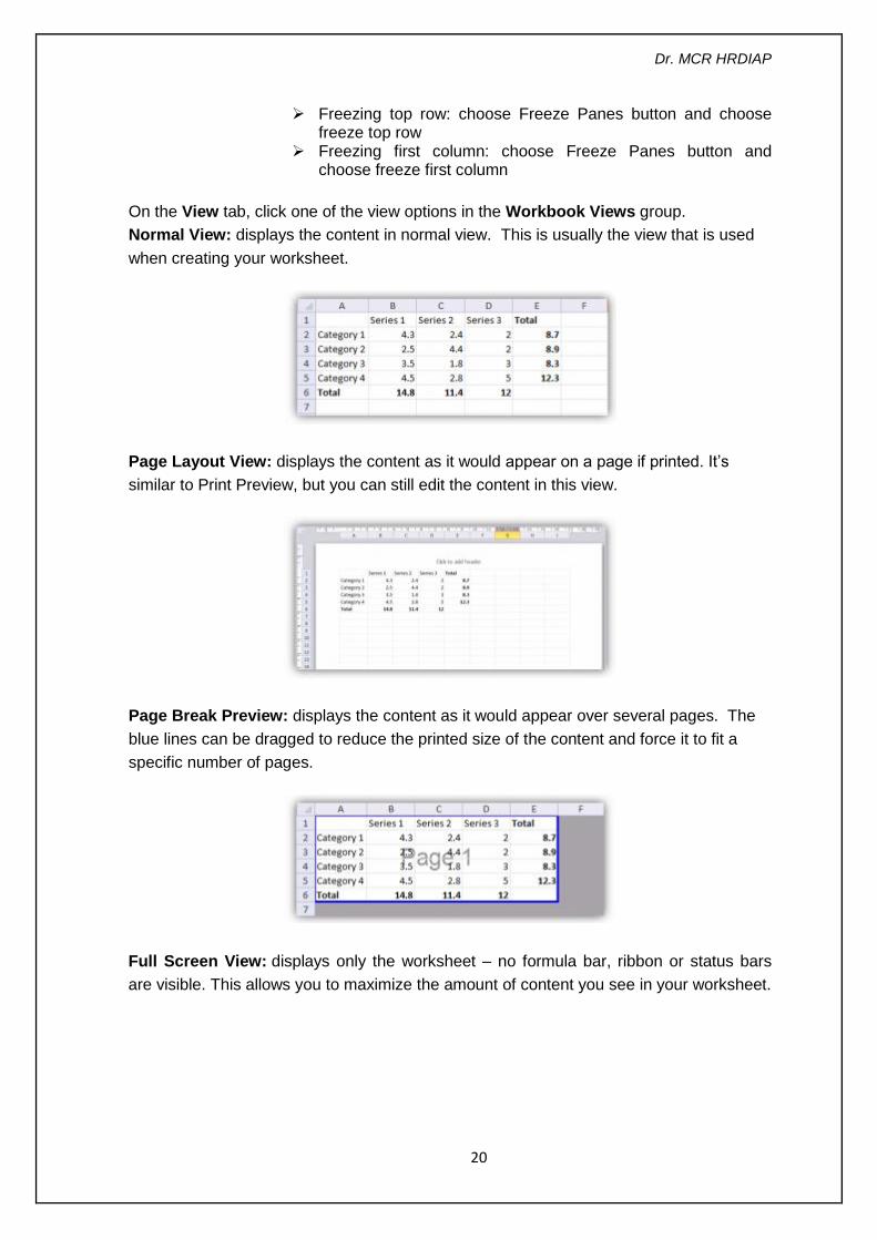
On the View tab, click one of the view options in the Workbook Views group.

Normal View: displays the content in normal view. This is usually the view that is used

when creating your worksheet.

Page Layout View: displays the content as it would appear on a page if printed. It’s

similar to Print Preview, but you can still edit the content in this view.

Page Break Preview: displays the content as it would appear over several pages. The

blue lines can be dragged to reduce the printed size of the content and force it to fit a

specific number of pages.

Full Screen View: displays only the worksheet – no formula bar, ribbon or status bars

are visible. This allows you to maximize the amount of content you see in your worksheet.

Dr. MCR HRDIAP

21

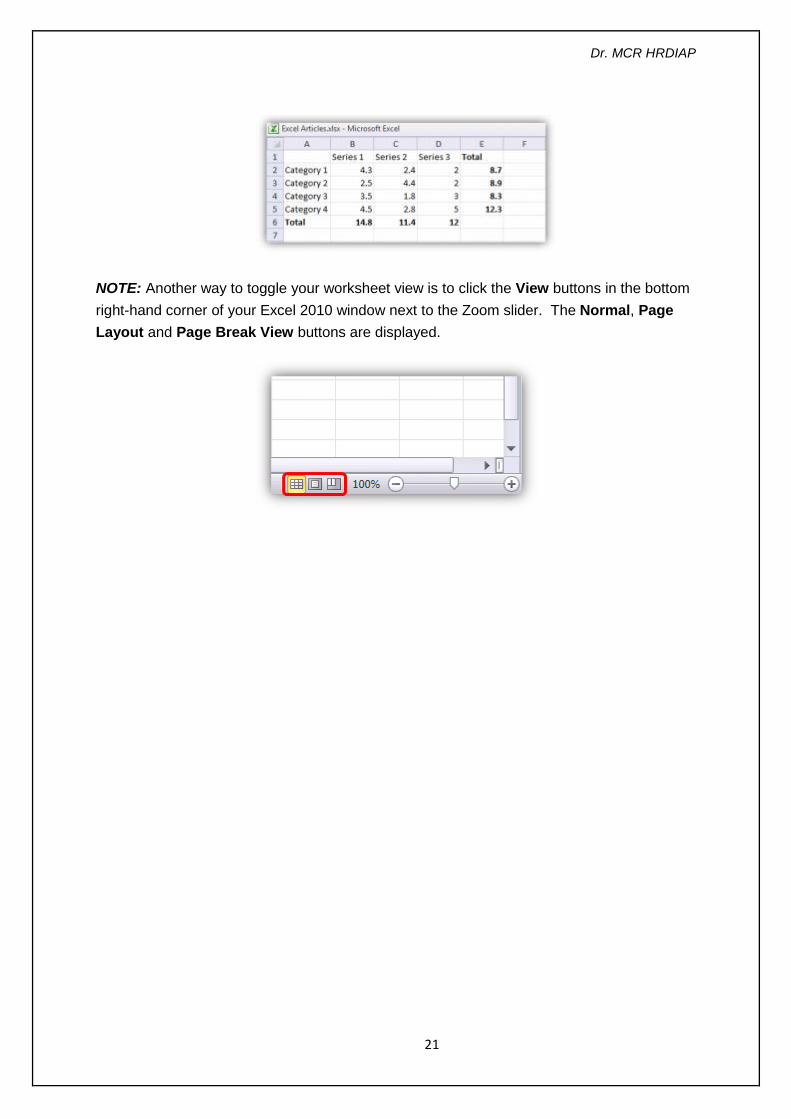
NOTE: Another way to toggle your worksheet view is to click the View buttons in the bottom

right-hand corner of your Excel 2010 window next to the Zoom slider. The Normal, Page

Layout and Page Break View buttons are displayed.

Dr. MCR HRDIAP

22

FUNCTIONS IN EXCEL 2.1 Enter function:

Select cell range Click on the function via menu shown on the right with ∑ Autosum in Editing

group under Home Tab. Or Select the cell in which you want to enter function value Enter symbol “=“ Enter function manually (e.g. “sum“), and cell range to which function will

apply. Most often used functions: =Sum(cell range)

adding the numbers in selected cells =Average(cell range)

finds medium number =Min(cell range)

finds the smallest value

=Max(cell range)

finds biggest value

=Count(cell range)

counts the number of records (only non-blank cells with numeric value)

=Counta(cell range)

counts the number of records (only non-blank cells with both alphabets and numeric value)

=Round(cell reference, nos. of decimal places)

This function rounds off the number upto given number of decimal places =SMALL(array, i) and

=LARGE(array, i)

This function SMALL returns the i-th smallest value from a given data set and the function LARGE returns the k-th largest from a given data set. You can use these two functions to estimate the relative standing of a particular value in a set of values. Where ‘array’ is the required argument and it is the numerical data set from which you want to find the k-th smallest value and the k-th largest value respectively. ‘i’ is also a required argument and it is the position in the data set or the array to be returned.

Dr. MCR HRDIAP

23

=RANK(number,ref,order)

Number: is the number whose rank you want to find. Ref: is an array of or a reference to a list of numbers. Non-numeric values in the array or the reference are ignored. Order: is a number specifying how to rank number.

2.2 Text functions =lower(Cell reference)

Converts the text into lower case

=upper(cell reference)

Converts the text into upper case

=len(cell reference)

Returns the number of characters the text contains

=concatenate(cell address1, cell address2, cell address3)

Combines the values of two or more cells

2.3 Date functions =today()

Inserts today’s date =now()

Inserts current date and time

2.4 PMT function

Excel 2010's PMT function calculates the periodic payment for an annuity, assuming a stream of equal payments and a constant rate of interest. The PMT function uses the following syntax:

=PMT(rate,nper,pv,[fv],[type])

As with the other common financial functions, rate is the interest rate per period, nper is the number of periods, pv is the present value or the amount the future payments are worth presently, fv is the future value or cash balance that you want after the last payment is made (Excel assumes a future value of zero when you omit this optional argument as you would when calculating loan payments), and type is the value 0 for payments made at the end of the period or the value 1 for payments made at the beginning of the period (if you omit the optional type argument, Excel assumes that the payment is made at the end of the period)

2.5 Logical function if

= logical function that compares the values in cells with some expression or a value.

Depending on the result we define the appropriate action

Syntax:

IF(logical _condition; value_if_true; value_if_false)

logical function checks if condition is met, and returns true or false

Dr. MCR HRDIAP

24

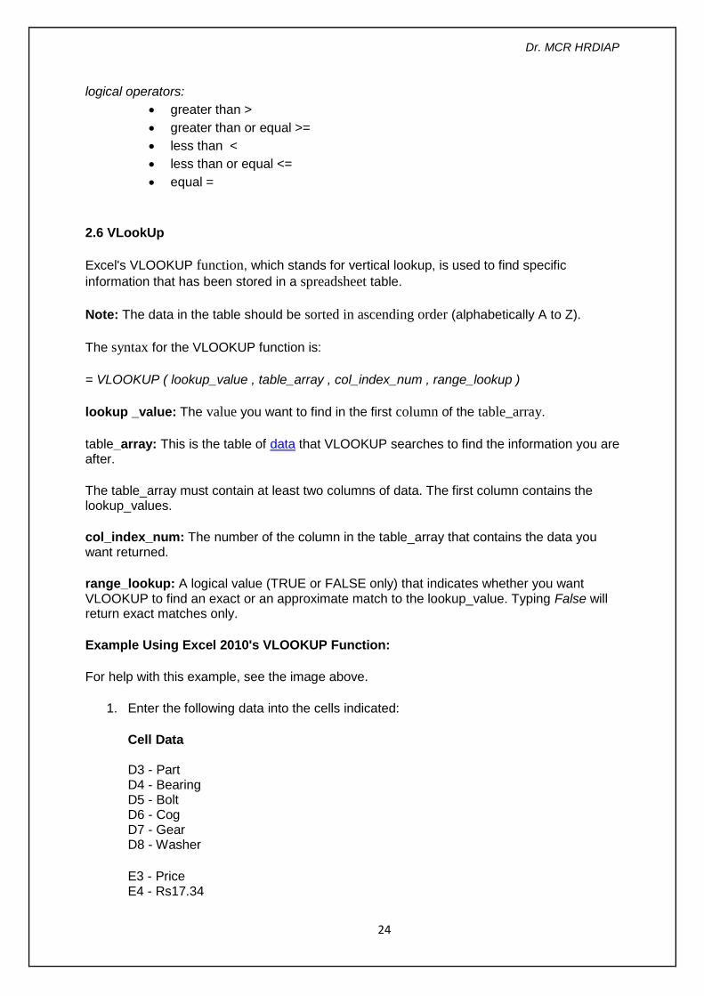
logical operators:

greater than >

greater than or equal >=

less than <

less than or equal <=

equal =

2.6 VLookUp

Excel's VLOOKUP function, which stands for vertical lookup, is used to find specific

information that has been stored in a spreadsheet table.

Note: The data in the table should be sorted in ascending order (alphabetically A to Z).

The syntax for the VLOOKUP function is:

= VLOOKUP ( lookup_value , table_array , col_index_num , range_lookup )

lookup _value: The value you want to find in the first column of the table_array.

table_array: This is the table of data that VLOOKUP searches to find the information you are after.

The table_array must contain at least two columns of data. The first column contains the lookup_values.

col_index_num: The number of the column in the table_array that contains the data you want returned.

range_lookup: A logical value (TRUE or FALSE only) that indicates whether you want VLOOKUP to find an exact or an approximate match to the lookup_value. Typing False will return exact matches only.

Example Using Excel 2010's VLOOKUP Function:

For help with this example, see the image above.

1. Enter the following data into the cells indicated:

Cell Data D3 - Part D4 - Bearing D5 - Bolt D6 - Cog D7 - Gear D8 - Washer

E3 - Price E4 - Rs17.34

Dr. MCR HRDIAP

25

E5 - Rs18.54 E6 - Rs20.21 E7 - Rs23.56 E8 - Rs11.43

2. Click on cell D1 and type the word Bolt. This is the part we are trying to price.

3. Click on cell E2 - the location where the results - in this case, the price of a bolt - will be displayed.

4. Click on the Formulas tab.

5. Choose Lookup & Reference from the ribbon to open the function drop down list.

6. Click on VLOOKUP in the list to bring up the function's dialog box.

7. In the dialog box, click on the Lookup _value line.

8. Click on cell D1 in the spreadsheet to tell VLOOKUP that we are looking for the price of bolts.

9. In the dialog box, click on the Table_array line.

10. Drag select cells D4 to E8 in the spreadsheet to enter that range into the dialog box.

The table_array is the table of data that VLOOKUP searches for the lookup_value specified in cell D1.

11. In the dialog box, click on the Col_index_num line.

12. Type the number 2 to indicate that the data we want returned is in column 2 of the table_array.

13. In the dialog box, click on the Range_lookup line.

14. Type the word False to indicate that we want an exact match for our requested data.

15. Click OK.

16. In cell D1 of the spreadsheet, type the word bolt.

17. The value Rs18.54 should appear in cell E1 displaying the price of a bolt as indicated in the table_array.

18. When you click on cell E1, the complete function = VLOOKUP ( D1 , D4:E8 , 2 , FALSE ) appears in the formula bar above the worksheet.

2.7 Formula referencing in Excel

Relative cell referencing

When formula is copied with AutoFill and formula have relative cell references, cell

references are going to adapt, for example:

If we use auto fill to copy following formula: =C5+B5 formula will change to: =C6+B6,

=C7+B7 etc.

Dr. MCR HRDIAP

26

Absolute cell referencing

If, in a formula, cell is referenced absolutely then applying autofill tool will result in:

=$C$5+B5, =$C$5+B6, =$C$5+B7 etc.

You can change selected cell reference from relative to absolute and vice versa using F4 key

Dr. MCR HRDIAP

27

MORE OPTIONS ON DATA 3.1 Deleting options

Clear All Clear Contents Clear Formats

3.2 Find & Replace

Find: enter a word or phrase and press Find button Replace:- Find What – field to enter word we search; Replace With - field to enter word that we want to use as replacement Format Painter - copy formatting from one part of the text to another Click on ?’ symbol to get Help in MS Excel or F1 on the keyboard

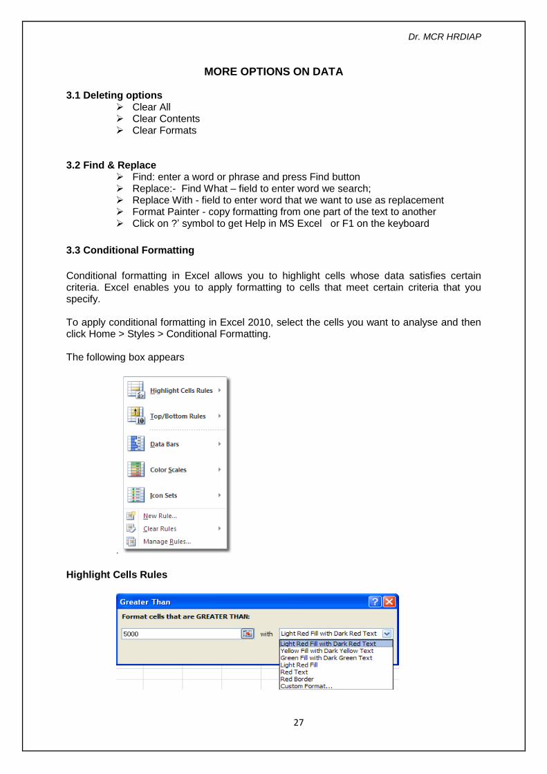
3.3 Conditional Formatting

Conditional formatting in Excel allows you to highlight cells whose data satisfies certain criteria. Excel enables you to apply formatting to cells that meet certain criteria that you specify.

To apply conditional formatting in Excel 2010, select the cells you want to analyse and then click Home > Styles > Conditional Formatting.

The following box appears

.

Highlight Cells Rules

Dr. MCR HRDIAP

28

3.4 Data Validation

Data validation is a feature available in Microsoft Excel. It allows you to do the following:

Make a list of the entries that restricts the values allowed in a cell. Create a prompt message explaining the kind of data allowed in a cell. Create messages that appear when incorrect data has been entered. Check for incorrect entries by using the Auditing toolbar. Set a range of numeric values that can be entered in a cell. Determine if an entry is valid based on calculation in another cell.

Make a List of Entries Allowed in the Cell You can make a list of the entries you will accept for a cell on a worksheet. You can then restrict the cell to accept only entries taken from the list by using the data validation feature. To create a drop-down list and restrict values in the cell to these entries, follow these steps:

1. Select cell A1. 2. On the Data menu, click Validation. 3. On the Settings tab, click List in the Allow drop-down list. 4. By default, the Ignore blank and In-cell Dropdown check boxes are selected. Do

not change them. 5. In the Source box, type a,b,c. Click OK.

NOTES: You can also enter a named range or cell reference if it contains a list of values. Both must be preceded by an equal sign. There is a 255 character limitation for this dialog.

Cell A1 now has a drop-down list next to it and you can use this list to select the value to enter in the cell.

Click the drop-down list and then click any item it contains.

This value will be entered in the cell.

NOTE: You can manually enter "a", "b", or "c", (without quotation marks) in the cell; you do not have to select these from the list. If you try to manually enter anything other these values, a stop message appears and you are unable to keep the value in this cell. Your only options are Retry or Cancel.

Set a Range of Numeric Values That Can Be Entered in a Cell You can place limits on the data that can be entered in a cell, you can set minimums and maximums or check for the effect an entry might have on another cell.

1. Select cell A5. 2. On the Data menu, click Validation and click the Settings tab. 3. In the Allow list, click Whole number. 4. In the Data list, click between. 5. In the Minimum box, enter 1. 6. In the Maximum box, enter 10.

NOTE: You can use cell references for Steps 5 and 6 to specify cells that contain the minimum and maximum values.

Dr. MCR HRDIAP

29

7. Click OK. 8. Enter the value 3 in cell A5. The value is entered without error. 9. Enter the value 33 in cell A5.

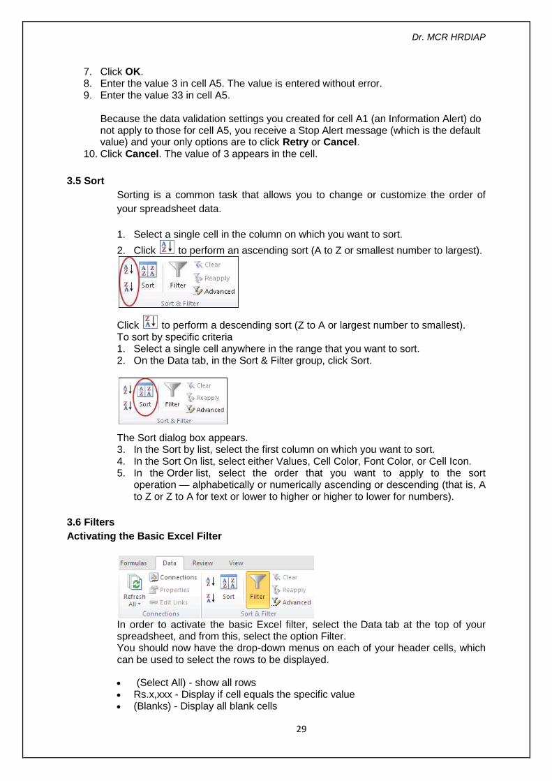
Because the data validation settings you created for cell A1 (an Information Alert) do not apply to those for cell A5, you receive a Stop Alert message (which is the default value) and your only options are to click Retry or Cancel.

10. Click Cancel. The value of 3 appears in the cell.

3.5 Sort

Sorting is a common task that allows you to change or customize the order of

your spreadsheet data.

1. Select a single cell in the column on which you want to sort.

2. Click to perform an ascending sort (A to Z or smallest number to largest).

Click to perform a descending sort (Z to A or largest number to smallest). To sort by specific criteria 1. Select a single cell anywhere in the range that you want to sort. 2. On the Data tab, in the Sort & Filter group, click Sort.

The Sort dialog box appears. 3. In the Sort by list, select the first column on which you want to sort. 4. In the Sort On list, select either Values, Cell Color, Font Color, or Cell Icon. 5. In the Order list, select the order that you want to apply to the sort

operation — alphabetically or numerically ascending or descending (that is, A to Z or Z to A for text or lower to higher or higher to lower for numbers).

3.6 Filters

Activating the Basic Excel Filter

In order to activate the basic Excel filter, select the Data tab at the top of your spreadsheet, and from this, select the option Filter. You should now have the drop-down menus on each of your header cells, which can be used to select the rows to be displayed.

(Select All) - show all rows Rs.x,xxx - Display if cell equals the specific value (Blanks) - Display all blank cells

Dr. MCR HRDIAP

30

The user can untick the values in rows that are not to be displayed.

Removing the Excel Filter To remove the filter simply select the Data tab at the top of your spreadsheet, and from within this, click on the Filter option.

3.7 Insert Subtotals in an Excel 2010 Worksheet

You can use Excel 2010's Subtotals feature to subtotal data in a sorted list. To subtotal a list, you first sort the list on the field for which you want the subtotals, and then you designate the field that contains the values you want summed — these don't have to be the same fields in the list.

. Steps to add subtotals to a list in a worksheet:

Sort the list on the field for which you want subtotals inserted. Click the Subtotal button in the Outline group on the Data tab.

The Subtotal dialog box appears.

Use the Subtotal dialog box to specify the options for the subtotals.

1. Select the field for which the subtotals are to be calculated in the At Each

Change In drop-down list.

2. Specify the type of totals you want to insert in the Use Function drop-down list.

3. Select the check boxes for the field(s) you want to total in the Add Subtotal To

list box.

4. Click OK.

Excel adds the subtotals to the worksheet.

3.8 Naming a Cell Range Assign a descriptive name to a cell or range in Excel 2010 to help make formulas in your

worksheets much easier to understand and maintain. Range names make it easier for you to

remember the purpose of a formula, rather than using obscure cell references. For example, the formula =SUM(Qtr2Sales) is much more intuitive than =SUM(C5:C12). In this example, you would assign the name Qtr2Sales to the range C5:C12 in the worksheet.

To name a cell or range, follow these steps:

1. Select the cell or cell range that you want to name. You also can select non- contiguous cells (press Ctrl as you select each cell or range).

Dr. MCR HRDIAP

31

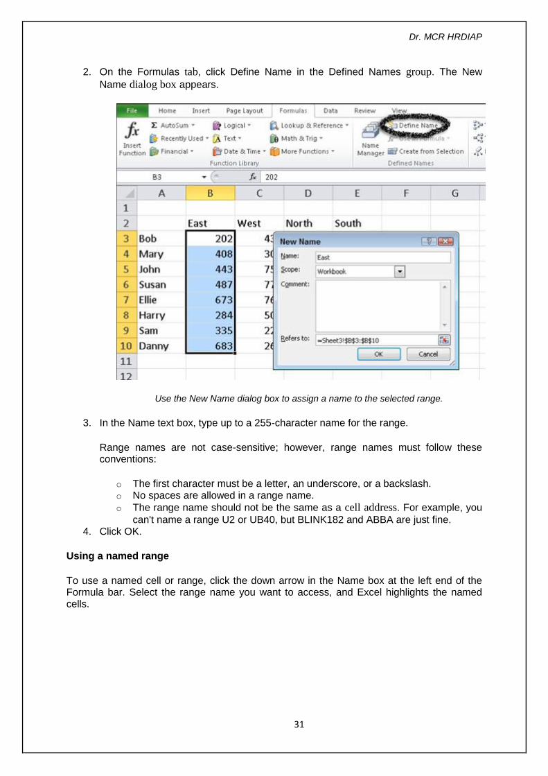
2. On the Formulas tab, click Define Name in the Defined Names group. The New

Name dialog box appears.

Use the New Name dialog box to assign a name to the selected range.

3. In the Name text box, type up to a 255-character name for the range.

Range names are not case-sensitive; however, range names must follow these conventions:

o The first character must be a letter, an underscore, or a backslash. o No spaces are allowed in a range name.

o The range name should not be the same as a cell address. For example, you

can't name a range U2 or UB40, but BLINK182 and ABBA are just fine. 4. Click OK.

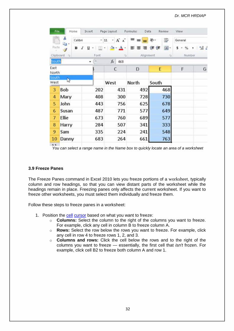
Using a named range

To use a named cell or range, click the down arrow in the Name box at the left end of the Formula bar. Select the range name you want to access, and Excel highlights the named cells.

Dr. MCR HRDIAP

32

You can select a range name in the Name box to quickly locate an area of a worksheet

3.9 Freeze Panes

The Freeze Panes command in Excel 2010 lets you freeze portions of a worksheet, typically

column and row headings, so that you can view distant parts of the worksheet while the headings remain in place. Freezing panes only affects the current worksheet. If you want to freeze other worksheets, you must select them individually and freeze them.

Follow these steps to freeze panes in a worksheet:

1. Position the cell cursor based on what you want to freeze: o Columns: Select the column to the right of the columns you want to freeze.

For example, click any cell in column B to freeze column A. o Rows: Select the row below the rows you want to freeze. For example, click

any cell in row 4 to freeze rows 1, 2, and 3. o Columns and rows: Click the cell below the rows and to the right of the

columns you want to freeze — essentially, the first cell that isn't frozen. For example, click cell B2 to freeze both column A and row 1.

Dr. MCR HRDIAP

33

Cells above and to the left of the current cell will be frozen.

2. In the Window group of the View tab, choose Freeze Panes→Freeze Panes.

A thin black line separates the sections. As you scroll down and to the right, notice that the columns above and rows to the left of the cell cursor remain fixed.

Keep titles visible by freezing the panes.

Normally when you press Ctrl+Home, Excel takes you to cell A1. However, when Freeze Panes is active, pressing Ctrl+Home takes you to the cell just below and to the right of the column headings. You can still use your arrow keys or click your mouse to access frozen cells.

3. In the Window group of the View tab, choose Freeze Panes→Unfreeze Panes to unlock the fixed rows and columns.

Dr. MCR HRDIAP

34

You can click the Freeze Top Row or Freeze First Column command in the Freeze Panes drop-down menu to freeze just the top row or first column in the worksheet, without regard to the position of the cell cursor in the worksheet.

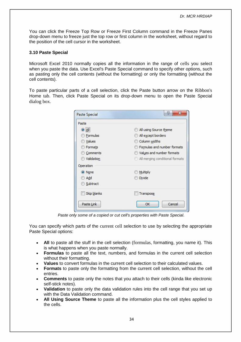
3.10 Paste Special

Microsoft Excel 2010 normally copies all the information in the range of cells you select

when you paste the data. Use Excel's Paste Special command to specify other options, such as pasting only the cell contents (without the formatting) or only the formatting (without the cell contents).

To paste particular parts of a cell selection, click the Paste button arrow on the Ribbon's

Home tab. Then, click Paste Special on its drop-down menu to open the Paste Special

dialog box.

Paste only some of a copied or cut cell's properties with Paste Special.

You can specify which parts of the current cell selection to use by selecting the appropriate

Paste Special options:

All to paste all the stuff in the cell selection (formulas, formatting, you name it). This

is what happens when you paste normally. Formulas to paste all the text, numbers, and formulas in the current cell selection

without their formatting. Values to convert formulas in the current cell selection to their calculated values. Formats to paste only the formatting from the current cell selection, without the cell

entries. Comments to paste only the notes that you attach to their cells (kinda like electronic

self-stick notes). Validation to paste only the data validation rules into the cell range that you set up

with the Data Validation command. All Using Source Theme to paste all the information plus the cell styles applied to

the cells.

Dr. MCR HRDIAP

35

All Except Borders to paste all the stuff in the cell selection without copying any borders you use there.

Column Widths to apply the column widths of the cells copied to the Clipboard to the columns where the cells are pasted.

Formulas and Number Formats to include the number formats assigned to the pasted values and formulas.

Values and Number Formats to convert formulas to their calculated values and include the number formats you assigned to all the copied or cut values.

All Merging Conditional Formats to paste conditional formatting into the cell range.

When you paste, you can also perform some simple math calculations based on the value(s) in the copied or cut cell(s) and the value in the target cell(s):

None: Excel performs no operation between the data entries you cut or copy to the Clipboard and the data entries in the cell range where you paste. This is the default setting.

Add: Excel adds the values you cut or copy to the Clipboard to the values in the cell range where you paste.

Subtract: Excel subtracts the values you cut or copy to the Clipboard from the values in the cell range where you paste.

Multiply: Excel multiplies the values you cut or copy to the Clipboard by the values in the cell range where you paste.

Divide: Excel divides the values you cut or copy to the Clipboard by the values in the cell range where you paste.

Finally, at the bottom of the Paste Special dialog box, you have a few other options:

Skip Blanks: Select this check box when you want Excel to paste only from the cells that aren't empty.

Transpose: Select this check box when you want Excel to change the orientation of the pasted entries. For example, if the original cells' entries run down the rows of a

single column of the worksheet, the transposed pasted entries will run across the

columns of a single row. Paste Link: Click this button when you want to establish a link between the copies

you're pasting and the original entries. That way, changes to the original cells automatically update in the pasted copies.

Dr. MCR HRDIAP

36

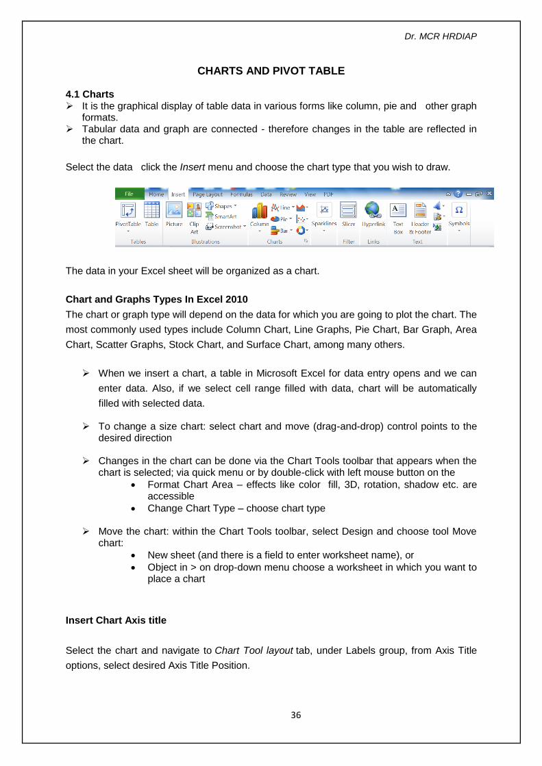
CHARTS AND PIVOT TABLE

4.1 Charts It is the graphical display of table data in various forms like column, pie and other graph

formats. Tabular data and graph are connected - therefore changes in the table are reflected in

the chart.

Select the data click the Insert menu and choose the chart type that you wish to draw.

The data in your Excel sheet will be organized as a chart.

Chart and Graphs Types In Excel 2010

The chart or graph type will depend on the data for which you are going to plot the chart. The

most commonly used types include Column Chart, Line Graphs, Pie Chart, Bar Graph, Area

Chart, Scatter Graphs, Stock Chart, and Surface Chart, among many others.

When we insert a chart, a table in Microsoft Excel for data entry opens and we can

enter data. Also, if we select cell range filled with data, chart will be automatically

filled with selected data.

To change a size chart: select chart and move (drag-and-drop) control points to the desired direction

Changes in the chart can be done via the Chart Tools toolbar that appears when the chart is selected; via quick menu or by double-click with left mouse button on the

Format Chart Area – effects like color fill, 3D, rotation, shadow etc. are accessible

Change Chart Type – choose chart type

Move the chart: within the Chart Tools toolbar, select Design and choose tool Move chart:

New sheet (and there is a field to enter worksheet name), or

Object in > on drop-down menu choose a worksheet in which you want to place a chart

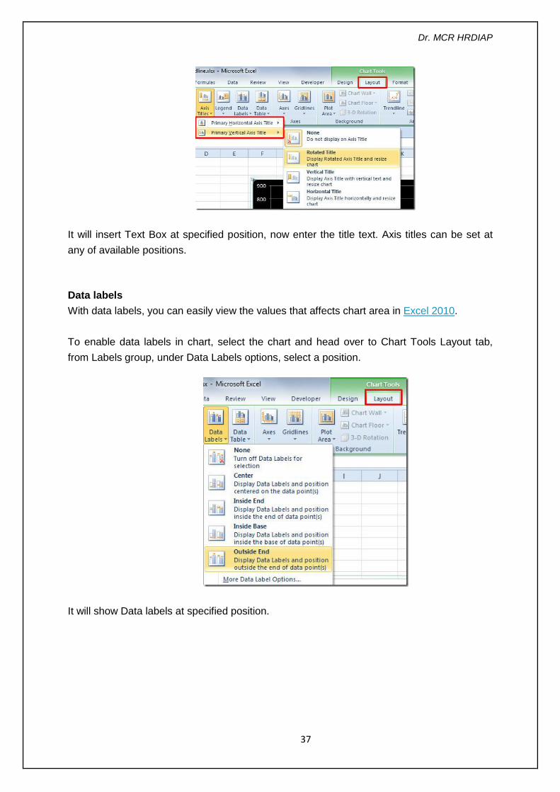
Insert Chart Axis title

Select the chart and navigate to Chart Tool layout tab, under Labels group, from Axis Title

options, select desired Axis Title Position.

Dr. MCR HRDIAP

37

It will insert Text Box at specified position, now enter the title text. Axis titles can be set at

any of available positions.

Data labels

With data labels, you can easily view the values that affects chart area in Excel 2010.

To enable data labels in chart, select the chart and head over to Chart Tools Layout tab,

from Labels group, under Data Labels options, select a position.

It will show Data labels at specified position.

Dr. MCR HRDIAP

38

4.2 Pivot Tables

A pivot table is a special type of summary table that's unique to Excel. Pivot tables are great

for summarizing values in a table because they do their magic without making you create

formulas to perform the calculations. Pivot tables also let you play around with the

arrangement of the summarized data. It's this capability of changing the arrangement of the summarized data on the fly simply by rotating row and column headings that gives the pivot table its name.

Follow these steps to create a pivot table:

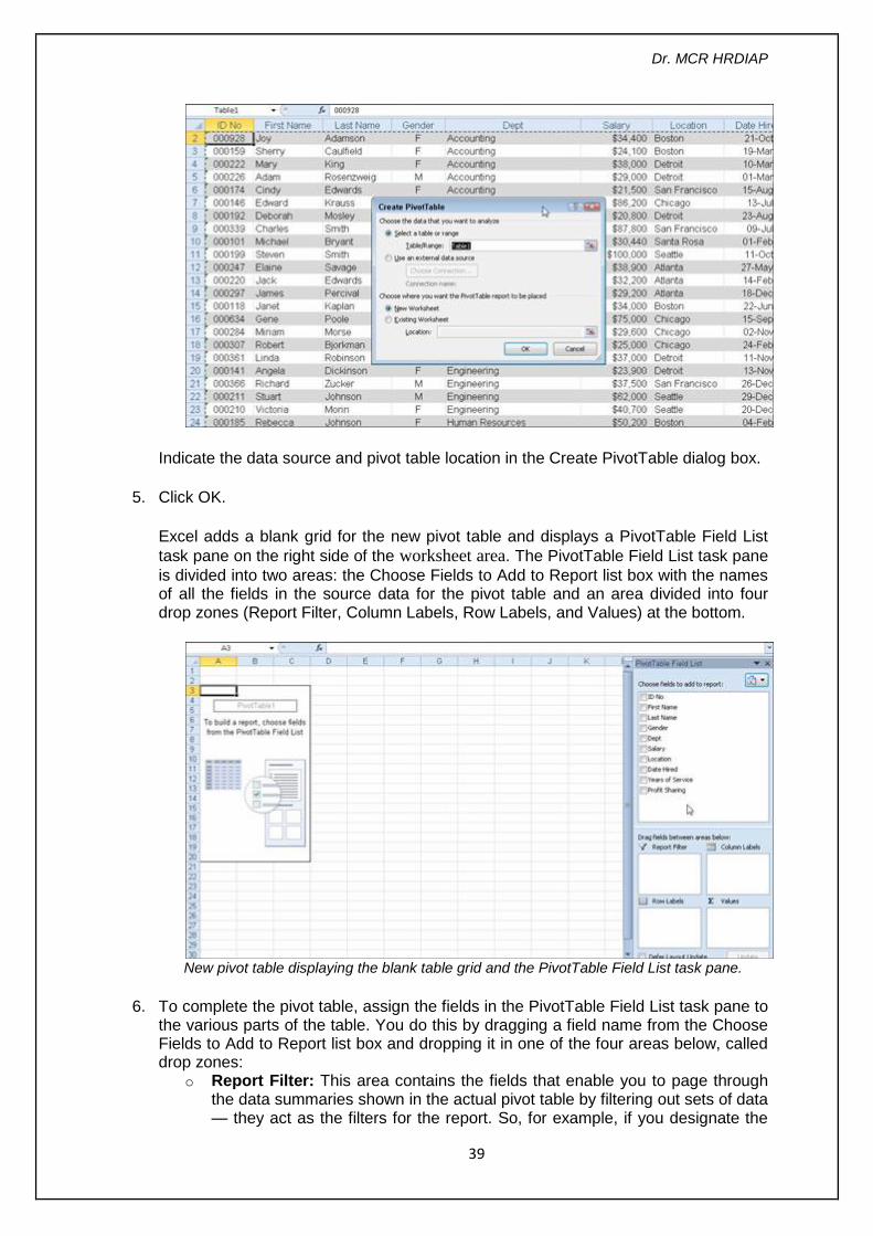
1. Open the worksheet that contains the table you want summarized by pivot table and

select any cell in the table.

Ensure that the table has no blank rows or columns and that each column has a header.

2. Click the PivotTable button in the Tables group on the Insert tab.

Click the top portion of the button; if you click the arrow, click PivotTable in the drop-

down menu. Excel opens the Create PivotTable dialog box and selects all the table

data, as indicated by a marquee around the cell range.

3. If necessary, adjust the range in the Table/Range text box under the Select a Table or Range option button.

If the data source for your pivot table is an external database table created with a separate program, such as Access, click the Use an External Data Source option button, click the Choose Connection button, and then click the name of the connection in the Existing Connections dialog box.

4. Select the location for the pivot table.

By default, Excel builds the pivot table on a new worksheet it adds to the workbook.

If you want the pivot table to appear on the same worksheet, click the Existing Worksheet option button and then indicate the location of the first cell of the new table in the Location text box.

Dr. MCR HRDIAP

39

Indicate the data source and pivot table location in the Create PivotTable dialog box.

5. Click OK.

Excel adds a blank grid for the new pivot table and displays a PivotTable Field List

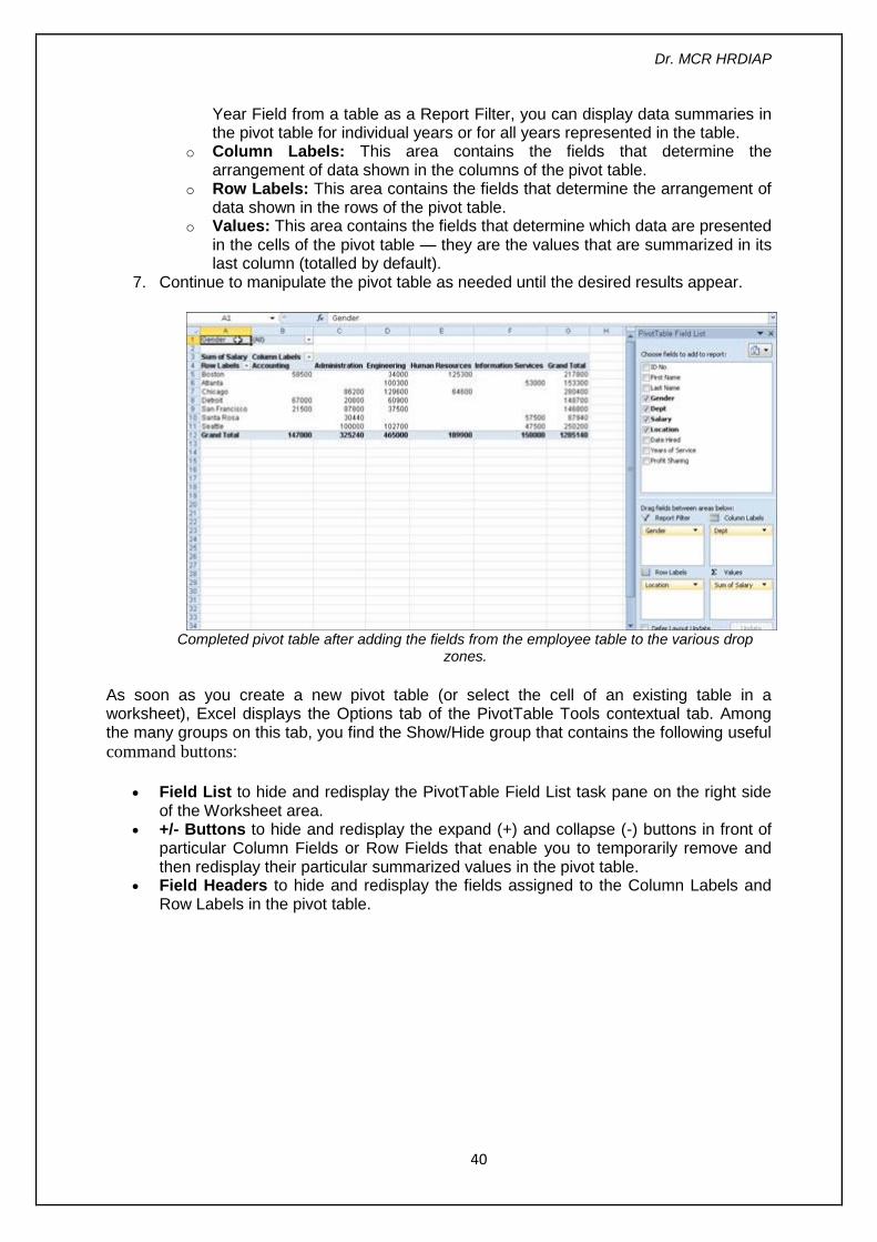
task pane on the right side of the worksheet area. The PivotTable Field List task pane

is divided into two areas: the Choose Fields to Add to Report list box with the names of all the fields in the source data for the pivot table and an area divided into four drop zones (Report Filter, Column Labels, Row Labels, and Values) at the bottom.

New pivot table displaying the blank table grid and the PivotTable Field List task pane.

6. To complete the pivot table, assign the fields in the PivotTable Field List task pane to the various parts of the table. You do this by dragging a field name from the Choose Fields to Add to Report list box and dropping it in one of the four areas below, called drop zones:

o Report Filter: This area contains the fields that enable you to page through the data summaries shown in the actual pivot table by filtering out sets of data — they act as the filters for the report. So, for example, if you designate the

Dr. MCR HRDIAP

40

Year Field from a table as a Report Filter, you can display data summaries in the pivot table for individual years or for all years represented in the table.

o Column Labels: This area contains the fields that determine the arrangement of data shown in the columns of the pivot table.

o Row Labels: This area contains the fields that determine the arrangement of data shown in the rows of the pivot table.

o Values: This area contains the fields that determine which data are presented in the cells of the pivot table — they are the values that are summarized in its last column (totalled by default).

7. Continue to manipulate the pivot table as needed until the desired results appear.

Completed pivot table after adding the fields from the employee table to the various drop zones.

As soon as you create a new pivot table (or select the cell of an existing table in a worksheet), Excel displays the Options tab of the PivotTable Tools contextual tab. Among the many groups on this tab, you find the Show/Hide group that contains the following useful

command buttons:

Field List to hide and redisplay the PivotTable Field List task pane on the right side of the Worksheet area.

+/- Buttons to hide and redisplay the expand (+) and collapse (-) buttons in front of particular Column Fields or Row Fields that enable you to temporarily remove and then redisplay their particular summarized values in the pivot table.

Field Headers to hide and redisplay the fields assigned to the Column Labels and Row Labels in the pivot table.

Dr. MCR HRDIAP

41

WHAT-IF-ANALYSIS AND MACROS

5.1 Scenario Manager

Excel 2010's Scenario Manager enables you to create and save sets of different input values that produce different calculated results as named scenarios (such as Best Case, Worst Case, and Most Likely Case). The key to creating the various scenarios for a table is to

identify the various cells in the data whose values can vary in each scenario. You then select

these cells (known as changing cells) in the worksheet before you open the Scenario

Manager dialog box.

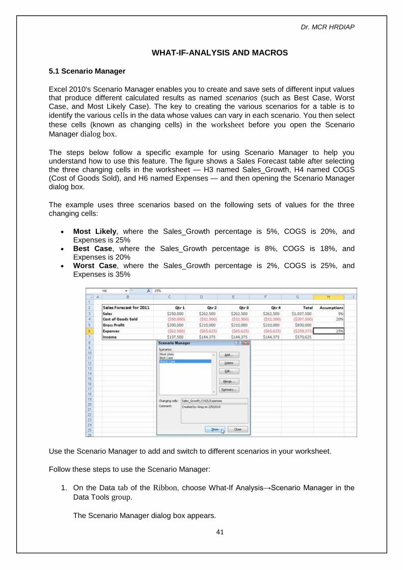
The steps below follow a specific example for using Scenario Manager to help you understand how to use this feature. The figure shows a Sales Forecast table after selecting the three changing cells in the worksheet — H3 named Sales_Growth, H4 named COGS (Cost of Goods Sold), and H6 named Expenses — and then opening the Scenario Manager dialog box.

The example uses three scenarios based on the following sets of values for the three changing cells:

Most Likely, where the Sales_Growth percentage is 5%, COGS is 20%, and Expenses is 25%

Best Case, where the Sales_Growth percentage is 8%, COGS is 18%, and Expenses is 20%

Worst Case, where the Sales_Growth percentage is 2%, COGS is 25%, and Expenses is 35%

Use the Scenario Manager to add and switch to different scenarios in your worksheet.

Follow these steps to use the Scenario Manager:

1. On the Data tab of the Ribbon, choose What-If Analysis→Scenario Manager in the

Data Tools group.

The Scenario Manager dialog box appears.

Dr. MCR HRDIAP

42

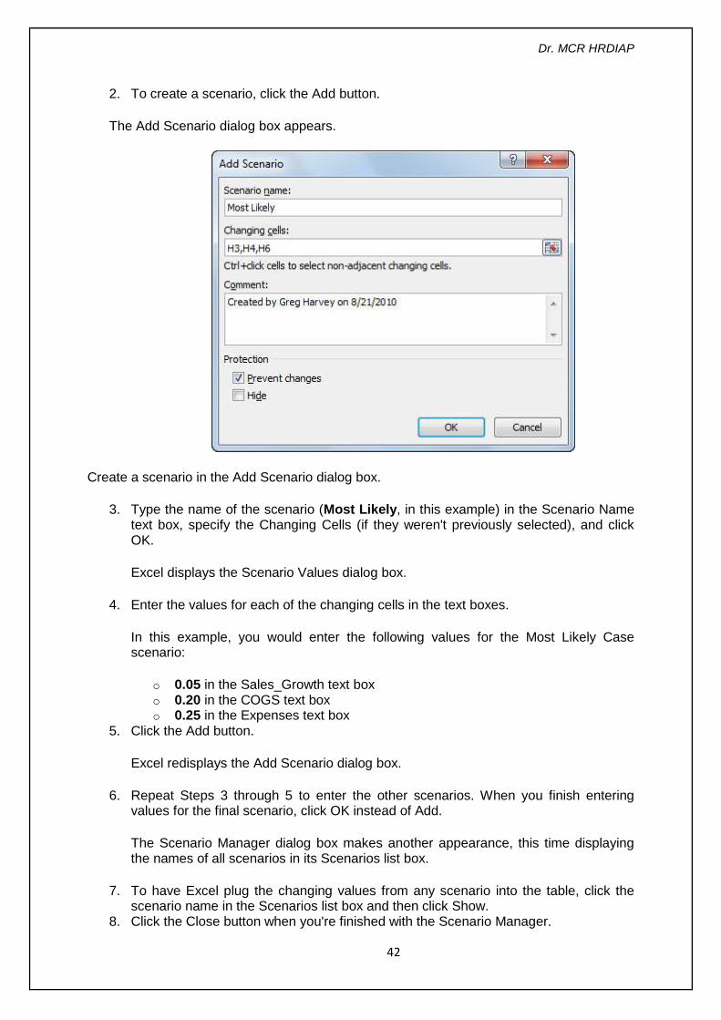
2. To create a scenario, click the Add button.

The Add Scenario dialog box appears.

Create a scenario in the Add Scenario dialog box.

3. Type the name of the scenario (Most Likely, in this example) in the Scenario Name text box, specify the Changing Cells (if they weren't previously selected), and click OK.

Excel displays the Scenario Values dialog box.

4. Enter the values for each of the changing cells in the text boxes.

In this example, you would enter the following values for the Most Likely Case scenario:

o 0.05 in the Sales_Growth text box o 0.20 in the COGS text box o 0.25 in the Expenses text box

5. Click the Add button.

Excel redisplays the Add Scenario dialog box.

6. Repeat Steps 3 through 5 to enter the other scenarios. When you finish entering values for the final scenario, click OK instead of Add.

The Scenario Manager dialog box makes another appearance, this time displaying the names of all scenarios in its Scenarios list box.

7. To have Excel plug the changing values from any scenario into the table, click the scenario name in the Scenarios list box and then click Show.

8. Click the Close button when you're finished with the Scenario Manager.

Dr. MCR HRDIAP

43

After adding the various scenarios for a table in your worksheet, don't forget to save the

workbook. That way, you'll have access to the various scenarios each time you open the

workbook in Excel by opening the Scenario Manager, selecting the scenario name, and clicking the Show button.

5.2 Goal Seek

The Goal Seek feature in Excel 2010 is a what-if analysis tool that enables you to find the

input values needed to achieve a goal or objective. To use Goal Seek, you select the cell

containing the formula that will return the result you're seeking and then indicate the target

value you want the formula to return and the location of the input value that Excel can change to reach the target.

The steps below follow a specific example for using Goal Seek to help you better understand how to use this feature. Refer to the figures for guidance. To use Goal Seek to find out how much sales must increase to return a net income of $300,000 in the first quarter, follow these steps:

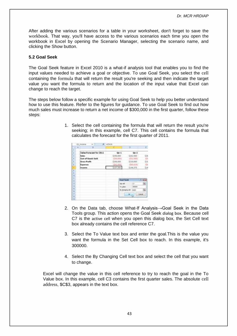
1. Select the cell containing the formula that will return the result you're seeking; in this example, cell C7. This cell contains the formula that calculates the forecast for the first quarter of 2011.

2. On the Data tab, choose What-If Analysis→Goal Seek in the Data Tools group. This action opens the Goal Seek dialog box. Because cell

C7 is the active cell when you open this dialog box, the Set Cell text

box already contains the cell reference C7.

3. Select the To Value text box and enter the goal.This is the value you

want the formula in the Set Cell box to reach. In this example, it's

300000.

4. Select the By Changing Cell text box and select the cell that you want

to change.

Excel will change the value in this cell reference to try to reach the goal in the To

Value box. In this example, cell C3 contains the first quarter sales. The absolute cell

address, $C$3, appears in the text box.

Dr. MCR HRDIAP

44

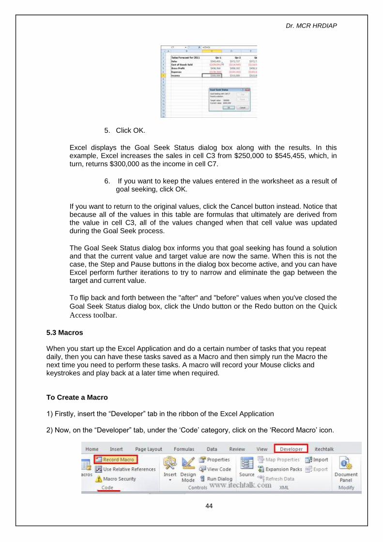
5. Click OK.

Excel displays the Goal Seek Status dialog box along with the results. In this example, Excel increases the sales in cell C3 from $250,000 to $545,455, which, in turn, returns $300,000 as the income in cell C7.

6. If you want to keep the values entered in the worksheet as a result of goal seeking, click OK.

If you want to return to the original values, click the Cancel button instead. Notice that because all of the values in this table are formulas that ultimately are derived from the value in cell C3, all of the values changed when that cell value was updated during the Goal Seek process.

The Goal Seek Status dialog box informs you that goal seeking has found a solution and that the current value and target value are now the same. When this is not the case, the Step and Pause buttons in the dialog box become active, and you can have Excel perform further iterations to try to narrow and eliminate the gap between the target and current value.

To flip back and forth between the "after" and "before" values when you've closed the

Goal Seek Status dialog box, click the Undo button or the Redo button on the Quick

Access toolbar.

5.3 Macros

When you start up the Excel Application and do a certain number of tasks that you repeat daily, then you can have these tasks saved as a Macro and then simply run the Macro the next time you need to perform these tasks. A macro will record your Mouse clicks and keystrokes and play back at a later time when required. To Create a Macro 1) Firstly, insert the “Developer” tab in the ribbon of the Excel Application 2) Now, on the “Developer” tab, under the ‘Code’ category, click on the ‘Record Macro’ icon.

Dr. MCR HRDIAP

45

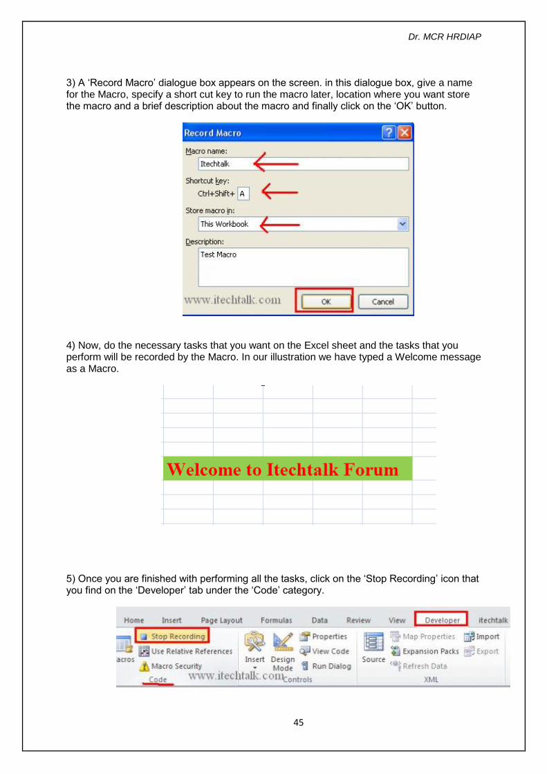
3) A ‘Record Macro’ dialogue box appears on the screen. in this dialogue box, give a name for the Macro, specify a short cut key to run the macro later, location where you want store the macro and a brief description about the macro and finally click on the ‘OK’ button.

4) Now, do the necessary tasks that you want on the Excel sheet and the tasks that you perform will be recorded by the Macro. In our illustration we have typed a Welcome message as a Macro.

5) Once you are finished with performing all the tasks, click on the ‘Stop Recording’ icon that you find on the ‘Developer’ tab under the ‘Code’ category.

Dr. MCR HRDIAP

46

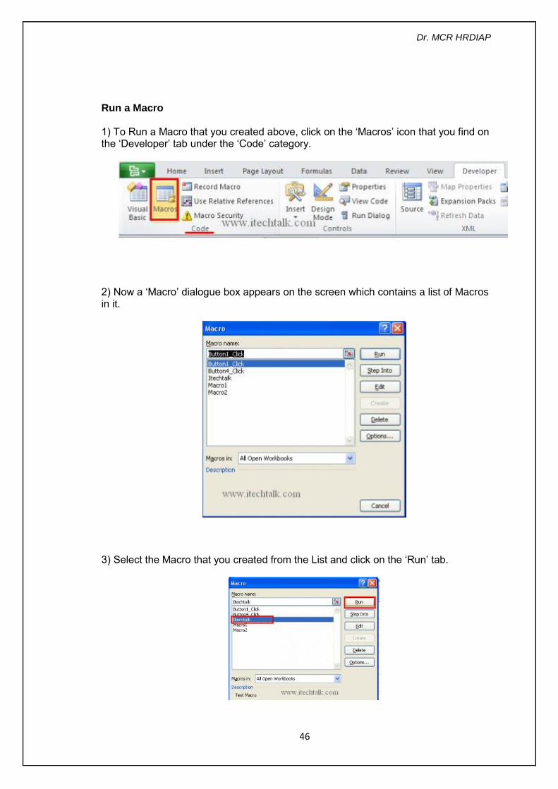
Run a Macro 1) To Run a Macro that you created above, click on the ‘Macros’ icon that you find on the ‘Developer’ tab under the ‘Code’ category.

2) Now a ‘Macro’ dialogue box appears on the screen which contains a list of Macros in it.

3) Select the Macro that you created from the List and click on the ‘Run’ tab.

Dr. MCR HRDIAP

47

PRINTING IN EXCEL

6.1 Printing Print worksheets, workbooks, and selections of cells. Prepare for printing by modifying page orientation, scale, margins, Print Titles, and page breaks.

Print Pane:

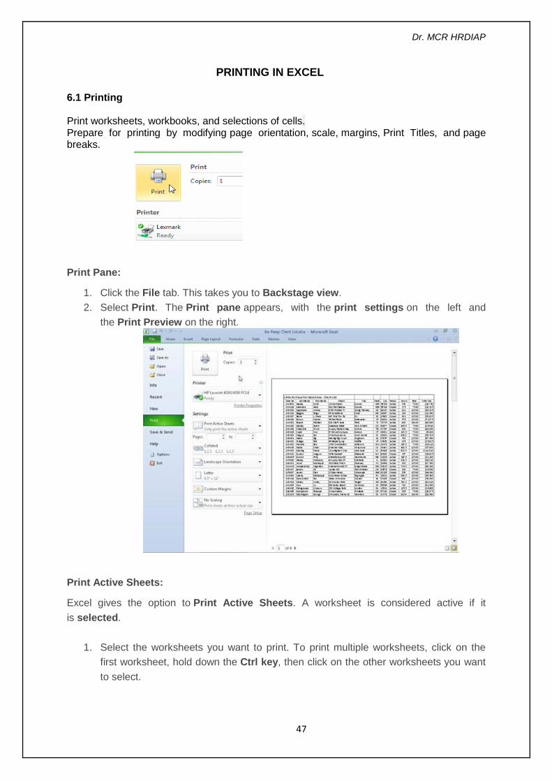
1. Click the File tab. This takes you to Backstage view.

2. Select Print. The Print pane appears, with the print settings on the left and

the Print Preview on the right.

Print Active Sheets:

Excel gives the option to Print Active Sheets. A worksheet is considered active if it

is selected.

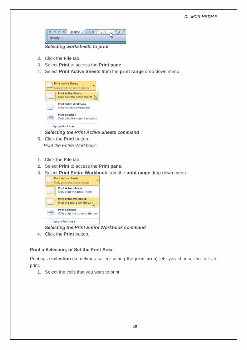
1. Select the worksheets you want to print. To print multiple worksheets, click on the

first worksheet, hold down the Ctrl key, then click on the other worksheets you want

to select.

Dr. MCR HRDIAP

48

Selecting worksheets to print

2. Click the File tab.

3. Select Print to access the Print pane.

4. Select Print Active Sheets from the print range drop-down menu.

Selecting the Print Active Sheets command

5. Click the Print button.

Print the Entire Workbook:

1. Click the File tab.

2. Select Print to access the Print pane.

3. Select Print Entire Workbook from the print range drop-down menu.

Selecting the Print Entire Workbook command

4. Click the Print button.

Print a Selection, or Set the Print Area:

Printing a selection (sometimes called setting the print area) lets you choose the cells to

print.

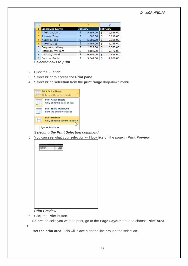
1. Select the cells that you want to print.

Dr. MCR HRDIAP

49

Selected cells to print

2. Click the File tab.

3. Select Print to access the Print pane.

4. Select Print Selection from the print range drop-down menu.

Selecting the Print Selection command

5. You can see what your selection will look like on the page in Print Preview.

Print Preview

6. Click the Print button.

Select the cells you want to print, go to the Page Layout tab, and choose Print Area-

>

set the print area. This will place a dotted line around the selection.

Dr. MCR HRDIAP

50

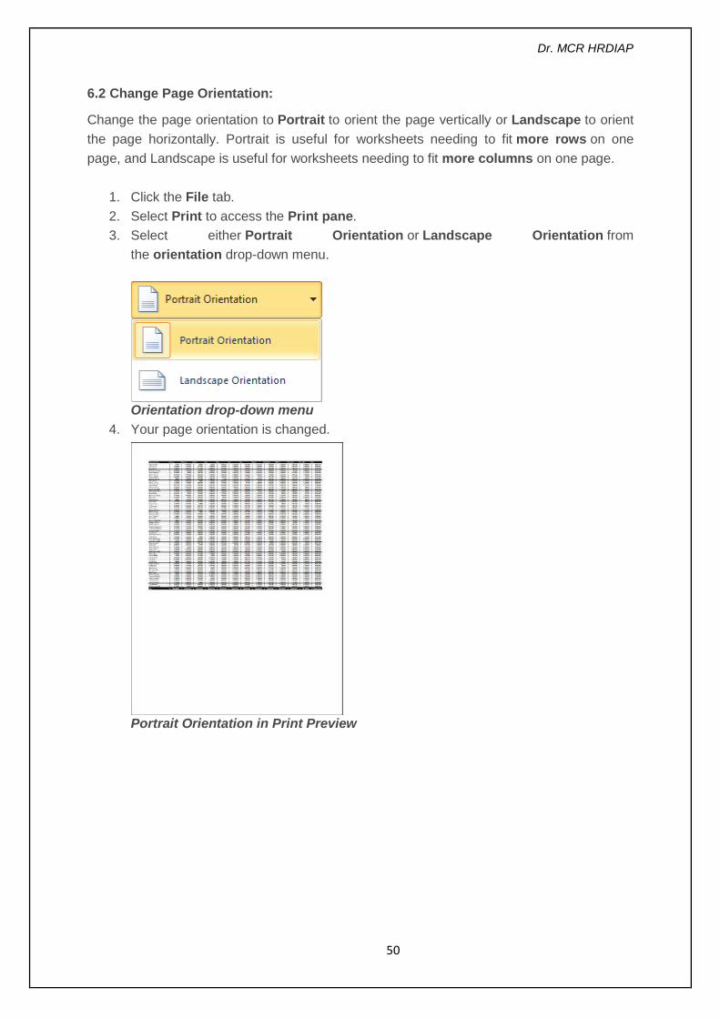
6.2 Change Page Orientation:

Change the page orientation to Portrait to orient the page vertically or Landscape to orient

the page horizontally. Portrait is useful for worksheets needing to fit more rows on one

page, and Landscape is useful for worksheets needing to fit more columns on one page.

1. Click the File tab.

2. Select Print to access the Print pane.

3. Select either Portrait Orientation or Landscape Orientation from

the orientation drop-down menu.

Orientation drop-down menu

4. Your page orientation is changed.

Portrait Orientation in Print Preview

Dr. MCR HRDIAP

51

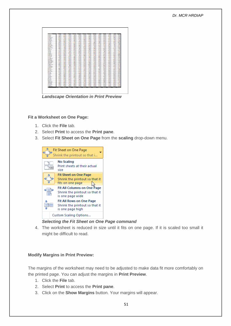
Landscape Orientation in Print Preview

Fit a Worksheet on One Page:

1. Click the File tab.

2. Select Print to access the Print pane.

3. Select Fit Sheet on One Page from the scaling drop-down menu.

Selecting the Fit Sheet on One Page command

4. The worksheet is reduced in size until it fits on one page. If it is scaled too small it

might be difficult to read.

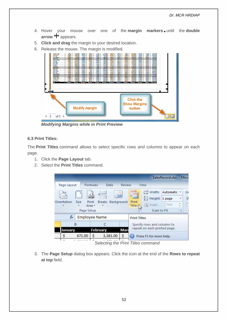
Modify Margins in Print Preview:

The margins of the worksheet may need to be adjusted to make data fit more comfortably on

the printed page. You can adjust the margins in Print Preview.

1. Click the File tab.

2. Select Print to access the Print pane.

3. Click on the Show Margins button. Your margins will appear.

Dr. MCR HRDIAP

52

4. Hover your mouse over one of the margin markers until the double

arrow appears.

5. Click and drag the margin to your desired location.

6. Release the mouse. The margin is modified.

Modifying Margins while in Print Preview

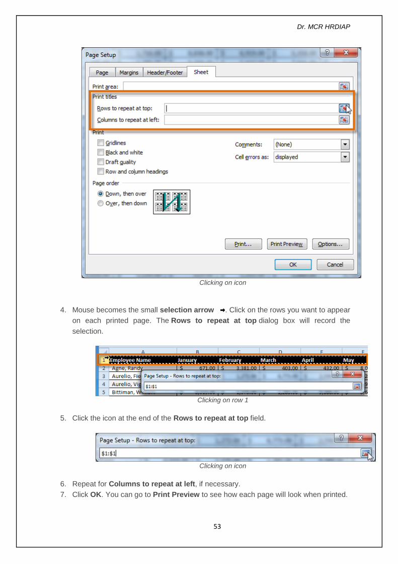
6.3 Print Titles:

The Print Titles command allows to select specific rows and columns to appear on each

page.

1. Click the Page Layout tab.

2. Select the Print Titles command.

Selecting the Print Titles command

3. The Page Setup dialog box appears. Click the icon at the end of the Rows to repeat

at top field.

Dr. MCR HRDIAP

53

Clicking on icon

4. Mouse becomes the small selection arrow . Click on the rows you want to appear

on each printed page. The Rows to repeat at top dialog box will record the

selection.

Clicking on row 1

5. Click the icon at the end of the Rows to repeat at top field.

Clicking on icon

6. Repeat for Columns to repeat at left, if necessary.

7. Click OK. You can go to Print Preview to see how each page will look when printed.

Dr. MCR HRDIAP

54

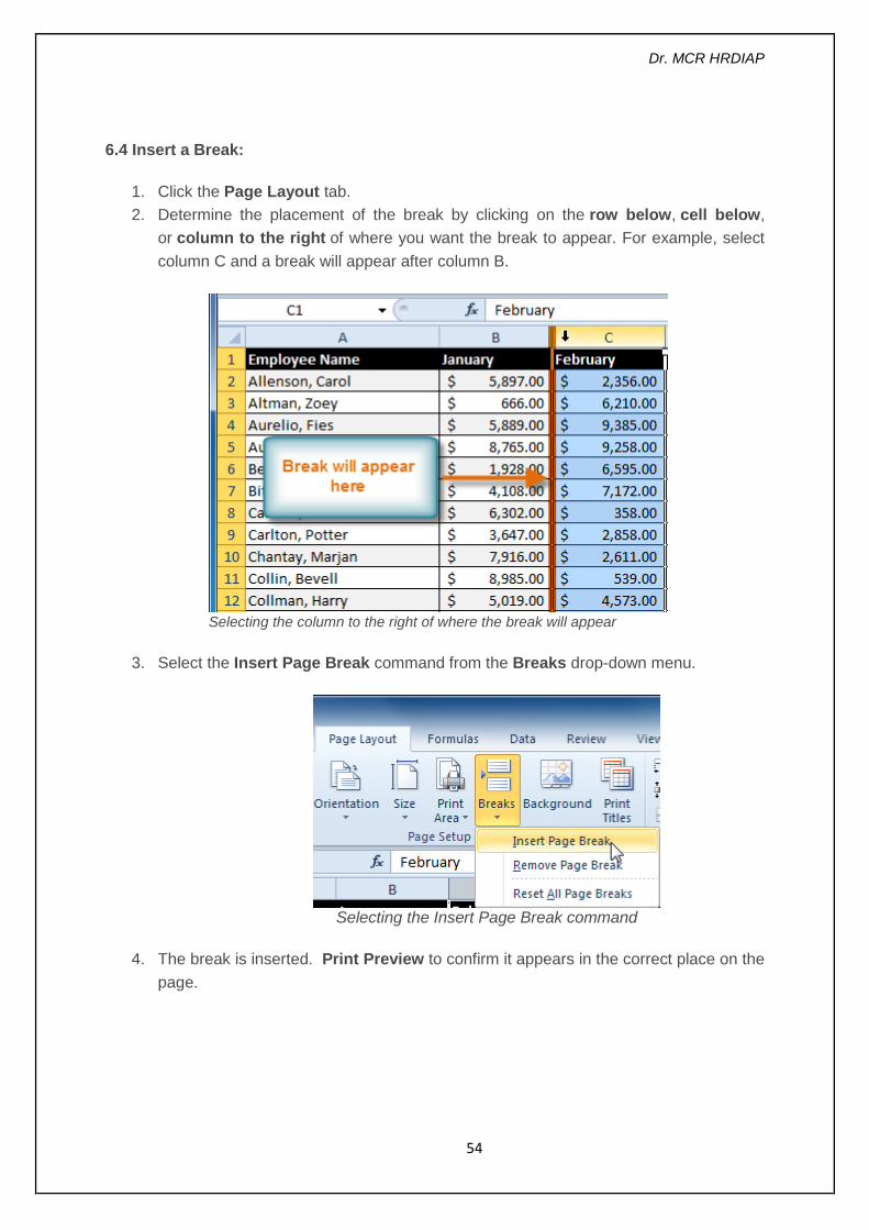
6.4 Insert a Break:

1. Click the Page Layout tab.

2. Determine the placement of the break by clicking on the row below, cell below,

or column to the right of where you want the break to appear. For example, select

column C and a break will appear after column B.

Selecting the column to the right of where the break will appear

3. Select the Insert Page Break command from the Breaks drop-down menu.

Selecting the Insert Page Break command

4. The break is inserted. Print Preview to confirm it appears in the correct place on the

page.

Dr. MCR HRDIAP

55

Dr. MCR HRDIAP

1