trace finite element methods for pdes on surfaces · trace finite element methods for pdes on...
TRANSCRIPT
Trace Finite Element Methods for PDEs on Surfaces
Maxim A. Olshanskii and Arnold Reusken
Institut für Geometrie und Praktische Mathematik Templergraben 55, 52062 Aachen, Germany
Maxim A. OlshanskiiDepartment of Mathematics, University of Houston, Houston, Texas 77204-3008, USA e-mail: [email protected]
Arnold ReuskenInstitut für Geometrie und Praktische Mathematik, RWTH Aachen University, D-52056 Aachen, Germany,e-mail: [email protected]
N O
V E
M B
E R
2
0 1
6
P R
E P
R I N
T
4 6
0
Trace Finite Element Methods for PDEs onSurfaces
Maxim A. Olshanskii and Arnold Reusken
Abstract In this paper we consider a class of unfitted finite element methods fordiscretization of partial differential equations on surfaces. In this class of methodsknown as the Trace Finite Element Method (TraceFEM), restrictions or traces ofbackground surface-independent finite element functions are used to approximatethe solution of a PDE on a surface. We treat equations on steady and time-dependent(evolving) surfaces. Higher order TraceFEM is explained in detail. We review theerror analysis and algebraic properties of the method. The paper navigates throughthe known variants of the TraceFEM and the literature on the subject.
1 Introduction
Consider the Laplace–Beltrami equation on a smooth closed surface Γ ,
−∆Γ u+u = f on Γ . (1)
Here ∆Γ is the Laplace–Beltrami operator on Γ . Equation (1) is an example of sur-face PDE, and it will serve as a model problem to explain the main principles ofthe TraceFEM. In this introduction we start with a brief review of the P1 TraceFEMfor (1), in which we explain the key ideas of this method. In this review paper thisbasic P1 finite element method applied to the model problem (1) on a stationary sur-face Γ will be extended to a general TraceFE methodology, including higher order
Maxim A. OlshanskiiDepartment of Mathematics, University of Houston, Houston, Texas 77204-3008, USA e-mail:[email protected]
Arnold ReuskenInstitut fur Geometrie und Praktische Mathematik, RWTH Aachen University, D-52056 Aachen,Germany e-mail: [email protected]
1
2 Maxim A. Olshanskii and Arnold Reusken
elements and surface approximations, time-dependent surfaces, adaptive methods,coupled problems, etc.
The main motivation for the development of the TraceFEM is the challenge ofbuilding an accurate and computationally efficient numerical method for surfacePDEs that avoids a triangulation of Γ or any other fitting of a mesh to the surface Γ .The method turns out to be particularly useful for problems with evolving surfaces inwhich the surface is implicitly given by a level set function. To discretize the partialdifferential equation on Γ , TraceFEM uses a surface independent background meshon a fixed bulk domain Ω ⊂R3, such that Γ ⊂Ω . The main concept of the method isto introduce a finite element space based on a volume triangulation (e.g., tetrahedraltessellation) of Ω , and to use traces of functions from this bulk finite element spaceon (an approximation of) Γ . The resulting trace space is used to define a finiteelement method for (1).
As an example, we consider the P1 TraceFEM for (1). Let Th be a consistentshape regular tetrahedral tessellation of Ω ⊂ R3 and let V bulk
h denote the standardFE space of continuous piecewise P1 functions w.r.t. Th. Assume Γ is given by thezero level of a C2 level set function φ , i.e., Γ = x ∈ Ω : φ(x) = 0. Consider theLagrangian interpolant φh ∈V bulk
h of φ and set
Γh := x ∈Ω : φh(x) = 0. (2)
Now we have an implicitly defined Γh, which is a polygonal approximation ofΓ . This Γh is a closed surface that can be partitioned in planar triangular segments:Γh =
⋃K∈Fh
K, where Fh is the set of all surface triangles. The bulk triangulation
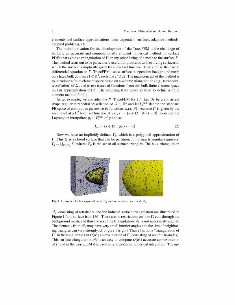
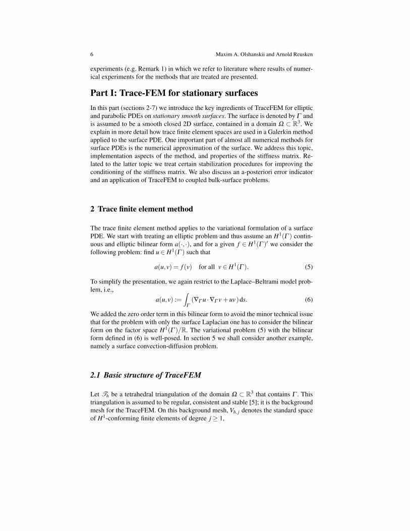
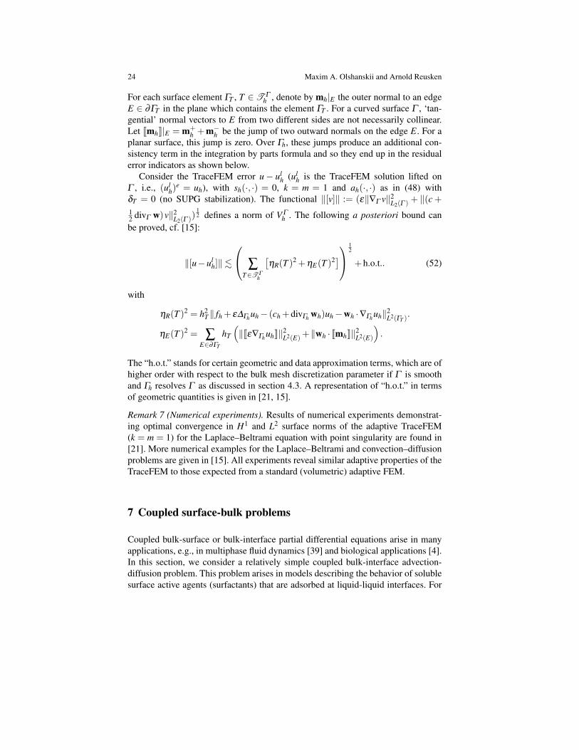
Fig. 1 Example of a background mesh Th and induced surface mesh Fh.
Th, consisting of tetrahedra and the induced surface triangulation are illustrated inFigure 1 for a surface from [56]. There are no restrictions on how Γh cuts through thebackground mesh, and thus the resulting triangulation Fh is not necessarily regular.The elements from Fh may have very small interior angles and the size of neighbor-ing triangles can vary strongly, cf. Figure 1 (right). Thus Γh is not a “triangulation ofΓ ” in the usual sense (an O(h2) approximation of Γ , consisting of regular triangles).This surface triangulation Fh is an easy to compute O(h2) accurate approximationof Γ and in the TraceFEM it is used only to perform numerical integration. The ap-

Trace Finite Element Methods for PDEs on Surfaces 3
proximation properties of the method entirely depend on the volumetric tetrahedralmesh Th. The latter is a fundamental property of the TraceFEM, as will be explainedin more detail in the remainder of this article.
As starting point for the finite element method we use a weak formulation of (1):Find u ∈ H1(Γ ) such that
∫Γ
uv+∇Γ u ·∇Γ v ds =∫
Γf v ds for all v ∈ H1(Γ ). Here
∇Γ is the tangential gradient on Γ . In the TraceFEM, in the weak formulation onereplaces Γ by Γh and instead of H1(Γh) uses the space of traces on Γh of all functionsfrom the bulk finite element space. The Galerkin formulation of (1) then reads: Finduh ∈V bulk
h such that∫Γh
uhvh +∇Γhuh ·∇Γhvh dsh =∫
Γh
fhvh dsh for all vh ∈Vbulk
h . (3)
Here fh is a suitable approximation of f on Γh. In the space of traces on Γh, VΓh :=
vh ∈ H1(Γh) |vh = vbulkh |Γh , vbulk
h ∈ V bulkh , the solution of (3) is unique. In other
words, although in general there are multiple functions uh ∈ V bulkh that satisfy (3),
the corresponding uh|Γh is unique. Furthermore, under reasonable assumptions thefollowing optimal error bound holds:
‖ue−uh‖L2(Γh)+h‖∇Γh(u
e−uh)‖L2(Γh)≤ ch2‖u‖H2(Γ ), (4)
where ue is a suitable extension of the solution to (1) off the surface Γ and h denotesthe mesh size of the outer triangulation Th. The constant c depends only on theshape regularity of Th and is independent of how the surface Γh cuts through thebackground mesh. This robustness property is extremely important for extendingthe method to time-dependent surfaces. It allows to keep the same background meshwhile the surface evolves through the bulk domain. One thus avoids unnecessarymesh fitting and mesh reconstruction.
A rigorous convergence analysis from which the result (4) follows will be givenfurther on (section 4). Here we already mention two interesting properties of theinduced surface triangulations which shed some light on why the method performsoptimally for such shape irregular surface meshes as illustrated in Figure 1. Theseproperties are the following: (i) If the background triangulation Th satisfies the min-imum angle condition, then the surface triangulation satisfies the maximum anglecondition [55]; (ii) Any element from Fh shares at least one vertex with a full sizeshape regular triangle from Fh [21].
For the matrix-vector representation of the TraceFEM one uses the nodal basisof the bulk finite element space V bulk
h rather than trying to construct a basis in VΓh .
This leads to singular or badly conditioned mass and stiffness matrices. In recentyears stabilizations have been developed which are easy to implement and result inmatrices with acceptable condition numbers. This linear algebra topic is treated issection 3.
In Part II of this article we explain how the ideas of the TraceFEM outlinedabove extend to the case of evolving surfaces. For such problems the method uses aspace–time framework, and the trial and test finite element spaces consist of tracesof standard volumetric elements on the space–time manifold. This manifold results

4 Maxim A. Olshanskii and Arnold Reusken
from the evolution of the surface. The method stays essentially Eulerian as a surfaceis not tracked by a mesh. Results of numerical tests show that the method applies,without any modifications and without stability restrictions on mesh or time stepsizes, to PDEs on surfaces undergoing topological changes. We believe that this isa unique property of TraceFEM among the state-of-the-art surface finite elementmethods.
1.1 Other surface Finite Element Methods
We briefly comment on other approaches known in the literature for solving PDEson surfaces. A detailed overview of different finite element techniques for surfacePDEs is given in [26]. The study of FEM for PDEs on general surfaces can betraced back to the paper of Dziuk [23]. In that paper, the Laplace–Beltrami equationis considered on a stationary surface Γ approximated by a regular family Γh ofconsistent triangulations. It is assumed that all vertices in the triangulations lie onΓ . The finite element space then consists of scalar functions that are continuous onΓh and linear on each triangle in the triangulation. The method is extended fromlinear to higher order finite elements in [19]. An adaptive finite element version ofthe method based on linear finite elements and suitable a posteriori error estimatorsare treated in [20]. More recently, Elliott and co-workers [24, 27, 30] developed andanalyzed an extension of the method of Dziuk for evolving surfaces. This surfacefinite element method is based on a Lagrangian tracking of the surface evolution.The surface Γ (t) is approximated by an evolving triangulated surface Γh(t). It isassumed that all vertices in the triangulation lie on Γ (t) and a given bulk velocityfield transports the vertices as material points (in the ALE variant of the method thetangential component of the transport velocity can be modified to assure a better dis-tribution of the vertices). The finite element space then consists of scalar functionsthat are continuous on Γh(t) and for each fixed t they are linear on each triangle inthe triangulation Γh(t). Only recently a higher order evolving surface FEM has beenstudied in [45]. If a surface undergoes strong deformations, topological changes, oris defined implicitly, e.g., as the zero level of a level set function, then numericalmethods based on such a Lagrangian approach have certain disadvantages.
In order to avoid remeshing and make full use of the implicit definition of thesurface as the zero of a level set function, it was first proposed in [3] to extend thepartial differential equation from the surface to a set of positive Lebesgue mea-sure in R3. The resulting PDE is then solved in one dimension higher but can besolved on a mesh that is unaligned to the surface. Such an extension approach isstudied in [2, 37, 69, 70] for finite difference approximations, also for PDEs onmoving surfaces. The extension approach can also be combined with finite elementmethods, see [6, 25, 58]. Another related method, which embeds a surface problemin a Cartesian bulk problem, is the closest point method of Ruuth and co-authors[48, 65, 61]. The method is based on using the closest point operator to extend theproblem from the surface to a small neighborhood of the surface, where standard
Trace Finite Element Methods for PDEs on Surfaces 5
Cartesian finite differences are used to discretize differential operators. The surfacePDE is then embedded and discretized in the neighborhood. Implementation re-quires the knowledge or calculation of the closest point on the surface for a givenpoint in the neighborhood. We are not aware of a finite element variant of the closestpoint method. Error analysis is also not known. The methods based on embeddinga surface PDE in a bulk PDE are known to have certain issues such as the need ofartificial boundary conditions and difficulties in handling geometrical singularities,see, e.g., the discussion in [37].
The TraceFEM that we consider in this article, or very closely related methods,are also called CutFEM in the literature, e.g. [9, 10, 11, 12]. Such CutFE techniqueshave originally been developed as unfitted finite element methods for interface prob-lems, cf. the recent overview paper [8]. In such a method applied to a model Poissoninterface problem one uses a standard finite element space on the whole domain andthen “cuts” the functions from this space at the interface, which is equivalent to tak-ing the trace of these functions on one of the subdomains (which are separated by theinterface). In our TraceFEM one also uses a “cut” of finite element functions fromthe bulk space, but now one cuts of the parts on both sides of the surface/interfaceand only keeps the part on the surface/interface. This explains why such trace tech-niques are also called Cut-FEM.
1.2 Structure of the article
The remainder of this article is divided into two parts. In the first part (sections 2-7)we treat different aspects of the TraceFEM for stationary elliptic PDEs on a station-ary surface. As model problem we consider the Laplace–Beltrami equation (1). Insection 2 we give a detailed explanation of the TraceFEM and also consider a higherorder isoparametric variant of the method. In section 3 important aspects related tothe matrix-vector representation of the discrete problem are treated. In particularseveral stabilization techniques are explained and compared. A discretization erroranalysis of TraceFEM is reviewed in section 4. Optimal (higher order) discretizationerror bounds are presented in that section. In section 5 we briefly treat a stabilizedvariant of TraceFEM that is suitable for convection dominated surface PDEs. Aresidual based a posteriori error indicator for the TraceFEM is explained in sec-tion 6. In the final section 7 of Part I the Trace- or Cut-FEM is applied for thediscretization of a coupled bulk-interface mass transport model.
In the second part (sections 8-11) we treat different aspects of the TraceFEM forparabolic PDEs on an evolving surface. In section 8 well-posedness of a space–timeweak formulation for a class of surface transport problems is studied. A space–timevariant of TraceFEM is explained in section 9 and some main results on stabilityand discretization errors for the method are treated in section 10. A few recentlydeveloped variants of the space–time TraceFEM are briefly addressed in section 11.
In view of the length of this article we decided not to present any results of nu-merical experiments. At the end of several sections we added remarks on numerical
6 Maxim A. Olshanskii and Arnold Reusken
experiments (e.g. Remark 1) in which we refer to literature where results of numer-ical experiments for the methods that are treated are presented.
Part I: Trace-FEM for stationary surfacesIn this part (sections 2-7) we introduce the key ingredients of TraceFEM for ellipticand parabolic PDEs on stationary smooth surfaces. The surface is denoted by Γ andis assumed to be a smooth closed 2D surface, contained in a domain Ω ⊂ R3. Weexplain in more detail how trace finite element spaces are used in a Galerkin methodapplied to the surface PDE. One important part of almost all numerical methods forsurface PDEs is the numerical approximation of the surface. We address this topic,implementation aspects of the method, and properties of the stiffness matrix. Re-lated to the latter topic we treat certain stabilization procedures for improving theconditioning of the stiffness matrix. We also discuss an a-posteriori error indicatorand an application of TraceFEM to coupled bulk-surface problems.
2 Trace finite element method
The trace finite element method applies to the variational formulation of a surfacePDE. We start with treating an elliptic problem and thus assume an H1(Γ ) contin-uous and elliptic bilinear form a(·, ·), and for a given f ∈ H1(Γ )′ we consider thefollowing problem: find u ∈ H1(Γ ) such that
a(u,v) = f (v) for all v ∈ H1(Γ ). (5)
To simplify the presentation, we again restrict to the Laplace–Beltrami model prob-lem, i.e.,
a(u,v) :=∫
Γ
(∇Γ u ·∇Γ v +uv)ds. (6)
We added the zero order term in this bilinear form to avoid the minor technical issuethat for the problem with only the surface Laplacian one has to consider the bilinearform on the factor space H1(Γ )/R. The variational problem (5) with the bilinearform defined in (6) is well-posed. In section 5 we shall consider another example,namely a surface convection-diffusion problem.
2.1 Basic structure of TraceFEM
Let Th be a tetrahedral triangulation of the domain Ω ⊂ R3 that contains Γ . Thistriangulation is assumed to be regular, consistent and stable [5]; it is the backgroundmesh for the TraceFEM. On this background mesh, Vh, j denotes the standard spaceof H1-conforming finite elements of degree j ≥ 1,
Trace Finite Element Methods for PDEs on Surfaces 7
Vh, j := vh ∈C(Ω) |vh|T ∈P j for all T ∈Th . (7)
The nodal interpolation operator in Vh, j is denoted by I j. We need an approximationΓh of Γ . Possible constructions of Γh and precise conditions that Γh has to satisfyfor the error analysis will be discussed later. For the definition of the method, it issufficient to assume that Γh is a Lipschitz surface without boundary. The active set oftetrahedra T Γ
h ⊂Th is defined by T Γh = T ∈Th : meas2(Γh∩T )> 0. If Γh∩T
consists of a face F of T , we include in T Γh only one of the two tetrahedra which
have this F as their intersection. The domain formed by the tetrahedra from T Γh
is denoted further by ωh. In the TraceFEM, only background degrees of freedomcorresponding to the tetrahedra from T Γ
h contribute to algebraic systems. Givena bulk (background) FE space of degree m, V bulk
h = Vh,m, the corresponding tracespace is
VΓh := vh|Γh : vh ∈V bulk
h . (8)
The trace space is a subspace of H1(Γh). On H1(Γh) one defines the finite elementbilinear form,
ah(u,v) :=∫
Γh
(∇Γhu ·∇Γhv+uv)dsh.
The form is coercive on H1(Γh), i.e. ah(uh,uh) ≥ ‖uh‖2L2(Γh)
holds. This guarantees
that the TraceFEM has a unique solution in VΓh . However, in TraceFEM formula-
tions we prefer to use the background space V bulkh rather than VΓ
h , cf. (3), (9) andfurther examples in this paper. There are several reasons for this choice. First ofall, in some versions of the method the volume information from trace elementsin ωh is used; secondly, for implementation one uses nodal basis functions fromV bulk
h to represent elements of VΓh ; thirdly, VΓ
h depends on the position of Γ , whileV bulk
h does not; and finally, the properties of V bulkh largely determine the properties
of the method. The trace space VΓh turns out to be convenient for the analysis of
the method. Thus, the basic form of the TraceFEM for the discretization of (6) is asfollows: Find uh ∈V bulk
h such that
ah(uh,vh) =∫
Γh
fhvh dsh for all vh ∈V bulkh . (9)
Here fh denotes an approximation of the data f on Γh. The construction of fh willbe discussed later, cf. Remark 4. Clearly, in (9) only the finite element functionsuh,vh ∈V bulk
h play a role which have at least one T ∈T Γh in their support.
2.2 Surface approximation and isoparametric TraceFEM
One major ingredient in the TraceFEM (as in many other numerical methods for sur-face PDEs) is a construction of the surface approximation Γh. Several methods fornumerical surface representation and approximation are known, cf. [26]. In this pa-

8 Maxim A. Olshanskii and Arnold Reusken
per we focus on the level set method for surface representation. As it is well-knownfrom the literature, the level set technique is a very popular method for surface rep-resentation, in particular for handling evolving surfaces.
Assume that the surface Γ is the zero level of a smooth level set function φ , i.e.,
Γ = x ∈Ω : φ(x) = 0. (10)
This level set function is not necessarily close to a signed distance function, but hasthe usual properties of a level set function: ‖∇φ(x)‖ ∼ 1, ‖D2φ(x)‖ ≤ c for all x ina neighborhood U of Γ . Assume that a finite element approximation φh ∈Vh,k of thefunction φ is available. If φ is sufficiently smooth, and one takes φh = Ik(φ), thenthe estimate
‖φ −φh‖L∞(U)+h‖∇(φ −φh)‖L∞(U) ≤ chk+1 (11)
defines the accuracy of the geometry approximation by φh. If φ is not known andφh is given, for example, as the solution to the level set equation, then an estimateas in (11) with some k ≥ 1 is often assumed in the error analysis of the TraceFEM.In section 4 we explain how the accuracy of the geometry recovery influences thediscretization error of the method. From the analysis we shall see that setting m = kfor the polynomial degree in background FE space and the discrete level set functionis the most natural choice.
The zero level of the finite element function φh (implicitly) characterizes an in-terface approximation Γh:
Γh = x ∈Ω : φh(x) = 0. (12)
With the exception of the linear case, k = 1, the numerical integration over Γh givenimplicitly in (12) is a non-trivial problem. One approach to the numerical integra-tion is based on an approximation of Γh within each T ∈T Γ
h by elementary shapes.Sub-triangulations or octree Cartesian meshes are commonly used for these pur-poses. On each elementary shape a standard quadrature rule is applied. The ap-proach is popular in combination with higher order XFEM, see, e.g., [1, 50, 22],and the level set method [49, 43]. Although numerically stable, the numerical in-tegration based on sub-partitioning may significantly increase the computationalcomplexity of a higher order finite element method. Numerical integration overimplicitly defined domains is a topic of current research, and in several recent pa-pers [51, 66, 32, 59, 44] techniques were developed that have optimal computationalcomplexity. Among those, the moment–fitting method from [51] can be appliedon 3D simplexes and, in the case of space–time methods, on 4D simplexes. Themethod, however, is rather involved and the weights computed by the fitting proce-dure are not necessarily positive. As a computationally efficient alternative, we willtreat below a higher order isoparamatric TraceFEM, which avoids the integrationover a zero level of φh.
The general framework of this paper, in particular the error analysis presented insection 4, provides an optimally accurate higher order method for PDEs on surfaces
Trace Finite Element Methods for PDEs on Surfaces 9
both for the isoparametric approach and for approaches that make use of a suitableintegration procedure on implicitly defined domain as in (12).
For piecewise linear polynomials a computationally efficient representation isstraightforward. To exploit this property, we introduce the piecewise linear nodalinterpolation of φh, which is denoted by φ lin
h = I1φh. Obviously, we have φ linh = φh
if k = 1. Furthermore, φ linh (xi) = φh(xi) at all vertices xi in the triangulation Th. A
lower order geometry approximation of the interface, which is very easy to deter-mine, is the zero level of this function:
Γlin := x ∈Ω | φ lin
h (x) = 0.
In most papers on finite element methods for surface PDEs the surface approxima-tion Γh = Γ lin is used. This surface approximation is piecewise planar, consistingof triangles and quadrilaterals. The latter can be subdivided into triangles. Hencequadrature on Γ lin can be reduced to quadrature on triangles, which is simple andcomputationally very efficient.
Recently in [46] a computationally efficient higher order surface approximationmethod has been introduced based on an isoparametric mapping. The approach from[46] can be used to derive an efficient higher order TraceFEM. We review the mainsteps below, while further technical details and analysis can be found in [34]. Weneed some further notation. All elements in the triangulation Th which are cut byΓ lin are collected in the set T Γlin
h := T ∈ Th | T ∩Γ lin 6= /0. The correspondingdomain is ω lin
h := x ∈ T | T ∈ T Γlinh . We introduce a mapping Ψ on ω lin
h withthe property Ψ(Γ lin) = Γ , which is defined as follows. Set G := ∇φ , and definea function d : ω lin
h → R such that d(x) is the smallest in absolute value numbersatisfying
φ(x+d(x)G(x)) = φlinh (x) for x ∈ ω
linh . (13)
For h sufficiently small the relation in (13) defines a unique d(x). Given the functiondG we define:
Ψ(x) := x+d(x)G(x), x ∈ ωlinh . (14)
From φ(Ψ(x)
)= φ lin
h (x) is follows that φ(Ψ(x)
)= 0 iff φ lin
h (x) = 0, and thusΨ(Γ lin) = Γ holds. In general, e.g., if φ is not explicitly known, the mapping Ψ
is not computable. We introduce an easy way to construct an accurate computableapproximation of Ψ , which is based on φh rather than on φ .
We define the polynomial extension ET : P(T )→P(R3) so that for v ∈ Vh,kwe have (ET v)|T = v|T , T ∈ T Γlin . For a search direction Gh ≈ G one needs asufficiently accurate approximation of ∇φ . One natural choice is
Gh = ∇φh,
but there are also other options. Given Gh we define a function dh : T Γlinh → R,
|dh| ≤ δ , with δ > 0 sufficiently small, as follows: dh(x) is the in absolute valuesmallest number such that

10 Maxim A. Olshanskii and Arnold Reusken
ET φh(x+dh(x)Gh(x)) = φlinh (x), for x ∈ T ∈T Γlin
h .
In the same spirit as above, corresponding to dh we define
Ψh(x) := x+dh(x)Gh(x), for x ∈ T ∈T Γlinh ,
which is an approximation of the mapping Ψ in (14). For any fixed x ∈ T Γlinh the
value Ψh(x) is easy to compute. The mapping Ψh may be discontinuous across facesand is not yet an isoparametric mapping. To derive an isoparametric mapping, de-noted by Θh below, one can use a simple projection Ph to map the transformation Ψhinto the continuous finite element space. For example, one may define Ph by averag-ing in a finite element node x, which requires only computing Ph(x) for all elementssharing x. This results in
Θh := PhΨh ∈ [Vh,k]3.
Based on this transformation one defines
Γh :=Θh(Γlin) = x ∈Ω : φ
linh(Θ−1h (x)
)= 0. (15)
The finite element mapping Θh is completely characterized by its values at the finiteelement nodes. These values can be determined in a computationally very efficientway. From this it follows that for Γh as in (15) we have a computationally efficientrepresentation. One can show that if (11) holds then for both Γh defined in (12) or(15) one gets (here and in the remainder the constant hidden in . does not dependon how Γ or Γh intersects the triangulation Th):
dist(Γh,Γ ) = maxx∈Γh
dist(x,Γ ). hk+1. (16)
For Γh defined in (15), however, we have a computationally efficient higher ordersurface approximation for all k ≥ 1. To allow an efficient quadrature in the Trace-FEM on Γh, one also has to transform the background finite element spaces Vh,m withthe same transformation Θh, as is standard in isoparametric finite element mehods.In this isoparametric TraceFEM, we apply the local transformation Θh to the spaceVh,m:
Vh,Θ = vh Θ−1h | vh ∈ (Vh,m)|ω lin
h= (vh Θ
−1h )|
Θh(ωlinh ) | vh ∈Vh,m . (17)
The isoparametric TraceFEM discretization now reads, compare to (9): Find uh ∈Vh,Θ such that∫
Γh
∇Γhuh ·∇Γhvh +uhvh dsh =∫
Γh
fhvh dsh for all vh ∈Vh,Θ , (18)
with Γh :=Θh(Γlin). Again, the method in (18) can be reformulated in terms of the
surface independent space V bulkh , see (19).
Trace Finite Element Methods for PDEs on Surfaces 11
To balance the geometric and approximation errors, it is natural to take m = k,i.e., the same degree of polynomials is used in the approximation φh of φ and in theapproximation uh of u. The isoparamatric TraceFEM is analyzed in [34] and optimalorder discretization error bounds are derived.
2.3 Implementation
We comment on an efficient implementation of the isoparamatric TraceFEM. Theintegrals in (18) can be evaluated based on numerical integration rules with respectto Γ lin and the transformation Θh. We illustrate this for the Laplacian part in thebilinear form. With uh = uh Θh, vh = vh Θh ∈V bulk
h :=Vh,m, there holds∫Γh
∇Γhuh ·∇Γhvh dsh =∫
Γ linPh(DΘh)
−T∇uh · Ph(DΘh)
−T∇vh JΓ dsh, (19)
where Ph = I− nhnTh is the tangential projection, nh = N/‖N‖ is the unit-normal
on Γh, N = (DΘh)−T nh, nh = ∇φ lin
h /‖∇φ linh ‖ is the normal with respect to Γ lin, and
JΓ = det(DΦh)‖N‖. This means that one only needs an accurate integration withrespect to the low order geometry Γ lin and the explicitly available mesh transforma-tion Θh ∈ [Vh,k]
3. The terms occuring in the integral on the right-hand side in (19)are polynomial functions on each triange element of Γ lin.
We emphasize that taking Vh,Θ in place of Vh,m in (18) is important. For Vh,mit is not clear how an efficient implementation can be realized. In that case oneneeds to integrate over ΓT := Γ lin ∩T (derivatives of) the function uh Θh, whereuh is piecewise polynomial on T ∈ Th. Due to the transformation Θh ∈ [Vh,k]
3 thefunction uh Θh has in general not more than only Lipschitz snoothness on ΓT .Hence an efficient and accurate quadrature becomes a difficult issue.
Remark 1 (Numerical experiments). Results of numerical experiments with theTraceFEM for P1 finite elements (m = 1) and a piecewise linear surface approxima-tion (k = 1) are given in [54]. Results for the higher order isoparametric TraceFEMare given in [34]. In that paper, results of numerical experiments with that methodfor 1≤ k = m≤ 5 are presented which confirm the optimal high order convergence.
3 Matrix-vector representation and stabilizations
The matrix-vector representation of the discrete problem in the TraceFEM dependson the choice of a basis (or frame) in the trace finite element space. The most nat-ural choice is to use the nodal basis of the outer space Vh,m for representation ofelements in the trace space VΓ
h . This choice has been used in almost all papers onTraceFEM. It, however, has some consequences. Firstly, in general the restrictions toΓh of the outer nodal basis functions on T Γ
h are not linear independent. Hence, these
12 Maxim A. Olshanskii and Arnold Reusken
functions only form a frame and not a basis of the trace finite element space, andthe corresponding mass matrix is singular. Often, however, the kernel of the massmatrix can be identified and is only one dimensional. Secondly, if one considersthe scaled mass matrix on the space orthogonal to its kernel, the spectral conditionnumber is typically not uniformly bounded with respect to h, but shows an O(h−2)growth. Clearly, this is different from the standard uniform boundedness propertyof mass matrices in finite element discretizations. Thirdly, both for the mass andstiffness matrix there is a dependence of the condition numbers on the location ofthe approximate interface Γh with respect to the outer triangulation. In certain “badintersection cases” the condition numbers can blow up. A numerical illustration ofsome of these effects is given in [52]. Results of numerical experiments indicatethat for scaled mass and stiffness matrices condition numbers become very large ifhigher order trace finite elements are used.
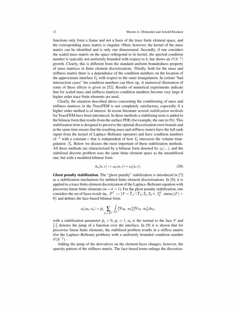
Clearly, the situation described above concerning the conditioning of mass andstiffness matrices in the TraceFEM is not completely satisfactory, especially if ahigher order method is of interest. In recent literature several stabilization methodsfor TraceFEM have been introduced. In these methods a stabilizing term is added tothe bilinear form that results from the surface PDE (for example, the one in (9)). Thisstabilization term is designed to preserve the optimal discretization error bounds andat the same time ensure that the resulting mass and stiffness matrix have the full rank(apart from the kernel of Laplace–Beltrami operator) and have condition numbersch−2 with a constant c that is independent of how Γh intersects the volume trian-gulation Th. Below we discuss the most important of these stabilization methods.All these methods are characterized by a bilinear form denoted by sh(·, ·), and thestabilized discrete problem uses the same finite element space as the unstabilizedone, but with a modified bilinear form
Ah(u,v) := ah(u,v)+ sh(u,v). (20)
Ghost penalty stabilization. The “ghost penalty” stabilization is introduced in [7]as a stabilization mechanism for unfitted finite element discretizations. In [9], it isapplied to a trace finite element discretization of the Laplace–Beltrami equation withpiecewise linear finite elements (m = k = 1). For the ghost penalty stabilization, oneconsiders the set of faces inside ωh, FΓ := F = T a∩T b;Ta,Tb ∈T Γ
h ,meas2(F)>0 and defines the face-based bilinear form
sh(uh,vh) = ρs ∑F∈FΓ
∫F[[∇uh ·nh]][[∇vh ·nh]]dsh,
with a stabilization parameter ρs > 0, ρs ' 1, nh is the normal to the face F and[[·]] denotes the jump of a function over the interface. In [9] it is shown that forpiecewise linear finite elements, the stabilized problem results in a stiffess matrix(for the Laplace–Beltrami problem) with a uniformly bounded condition numberO(h−2).
Adding the jump of the derivatives on the element-faces changes, however, thesparsity pattern of the stiffness matrix. The face-based terms enlarge the discretiza-
Trace Finite Element Methods for PDEs on Surfaces 13
tion stencils. To our knowledge, there is no higher order version of the ghost penaltymethod for surface PDEs which provides a uniform bound on the condition number.Full gradient surface stabilization. The “full gradient” stabilization is a methodwhich does not rely on face-based terms and keeps the sparsity pattern intact. It wasintroduced in [18, 63]. The bilinear form which describes this stabilization is
sh(uh,vh) :=∫
Γh
∇uh ·nh ∇vh ·nh dsh, (21)
where nh denotes the normal to Γh. Thus, we get Ah(uh,vh) =∫
Γh(∇uh ·∇vh +
uhvh)dsh, which explains the name of the method. The stabilization is very easyto implement.
For the case of linear finite elements, it is shown in [63] that one has a uniformcondition number bound O(h−2). For the case of higher order TraceFEM (m >1), full gradient stabilization does not result in a uniform bound on the conditionnumber, cf. [63, Remark 6.5].Full gradient volume stabilization. Another “full gradient” stabilization was intro-duced in [11]. It uses the full gradient in the volume instead of only on the surface.The stabilization bilinear form is
sh(uh,vh) = ρs
∫ΩΓ
Θ
∇uh ·∇vhdx,
with a stabilization parameter ρs > 0, ρs' h. For Γh =Γ lin the domain ΩΓΘ
is just theunion of tetrahedra intersected by Γh. For application to an isoparametric TraceFEMas treated in section 2.2 one should use the transformed domain ΩΓ
Θ:= Θh(ω
linh ).
This method is easy to implement as its bilinear form is provided by most finiteelement codes. Using the analysis from [11, 34] it can be shown that a uniform con-dition number bound O(h−2) holds not only for linear finite elements but also forthe higher order isoparametric TraceFEM. However, the stabilization is not “suffi-ciently consistent”, in the sense that for the stabilized method one does not have theoptimal order discretization bound for m > 1.Normal derivative volume stabilization. In the lowest-order case m = 1, all threestabilization methods discussed above result in a discretization which has a dis-cretization error of optimal order and a stiffness matrix with a uniform O(h−2)condition number bound. However, none of these methods has both properties alsofor m > 1. We now discuss a recently introduced stabilization method [34], whichdoes have both properties for arbitrary m≥ 1. Its bilinear form is given by
sh(uh,vh) := ρs
∫ΩΓ
Θ
nh ·∇uh nh ·∇vh dx, (22)
with ρs > 0 and nh the normal to Γh, which can easily be determined. This is a naturalvariant of the full gradient stabilizations treated above. As in the full gradient surfacestabilization only normal derivatives are added, but this time (as in the full gradientvolume stabilization) in the volume ΩΓ
Θ. The implementation of this stabilization
14 Maxim A. Olshanskii and Arnold Reusken
term is fairly simple as it fits well into the structure of many finite element codes. Itcan be shown, see [34], that using this stabilization in the isoparametric TraceFEMone obtains, for arbitrary m = k ≥ 1, optimal order discretization bounds, and theresulting stiffness matrix has a spectral condition number ch−2, where the constantc does not depend on the position of the surface approximation Γh in the triangula-tion Th. For these results to hold, one can take the scaling paremater ρs from thefollowing (very large) parameter range:
h . ρs . h−1. (23)
Results of numerical experiments with illustrate the dependence of discretizationerrors and condition numbers on ρs are given in [34].
4 Discretization error analysis
In this section we present a general framework in which both optimal order dis-cretization bounds can be established and the conditioning of the resulting stiffnessmatrix can be analyzed. Our exposition follows the papers [63, 34]. In this frame-work we need certain ingredients such as approximation error bounds for the finiteelement spaces, consistency estimates for the geometric error and certain fundamen-tal properties of the stabilization. The required results are scattered in the literatureand can be found in many papers, some of which we refer to below.
For the discretization we need an approximation Γh of Γ . We do not specify aparticular construction for Γh at this point, but only assume certain properties intro-duced in section 4.1 below. This Γh may, for example, be constructed via a mappingΘh as section 2.2, i.e., Γh =Θh(Γ
lin) or it may be characterized as the zero level of a(higher order) level set function φh, cf. (12). In the latter case, to perform quadratureon Γh one does not use any special transformation but applies a “direct” procedure,e.g., a subpartioning technique or the moment-fitting method. This difference (directaccess to Γh or access via Θh) has to be taken into account in the definition of thetrace spaces. We want to present an analysis which covers both cases and thereforewe introduce a local bijective mapping Φh, which is either Φh =Θh (Γh is accessedvia transformation Θh), cf. (17), or Φh = id (direct access to Γh) and define
Vh,Φ := (vh Φ−1h )|ΩΓ
Φ
| vh ∈Vh,m ,
where ΩΓΦ
is the domain formed by all (transformed) tetrahedra that are intersectedby Γh.
We consider the bilinear form Ah from (20) with a general symmetric positivesemidefinite bilinear form sh(·, ·). Examples of sh(·, ·) are sh ≡ 0 (no stabilization)and the ones discussed in section 3. The discrete problem is as follows: Find uh ∈Vh,Φ such that
Ah(uh,vh) =∫
Γh
fhvh dsh for all vh ∈Vh,Φ . (24)
Trace Finite Element Methods for PDEs on Surfaces 15
In the sections below we present a general framework for discretization error anal-ysis of this method and outline main results. Furthermore the conditioning of theresulting stiffness matrix is studied.
4.1 Preliminaries
We collect some notation and results that we need in the error analysis. We alwaysassume that Γ is sufficiently smooth without specifying the regularity of Γ . Thesigned distance function to Γ is denoted by d, with d negative in the interior of Γ .On Uδ := x ∈ R3 : |d(x)|< δ , with δ > 0 sufficiently small, we define
n(x) = ∇d(x), H(x) = D2d(x), P(x) = I−n(x)n(x)T , (25)p(x) = x−d(x)n(x), ve(x) = v(p(x)) for v defined on Γ . (26)
The eigenvalues of H(x) are denoted by κ1(x),κ2(x) and 0. Note that ve is simply theconstant extension of v (given on Γ ) along the normals n. The tangential derivativecan be written as ∇Γ g(x)=P(x)∇g(x) for x∈Γ . We assume δ0 > 0 to be sufficientlysmall such that on Uδ0 the decomposition
x = p(x)+d(x)n(x)
is unique for all x ∈Uδ0 . In the remainder we only consider Uδ with 0 < δ ≤ δ0. Inthe analysis we use basic transformation formulas (see, e.g.,[20]). For example:
∇ue(x) = (I−d(x)H(x))∇Γ u(p(x)) a.e on Uδ0 , u ∈ H1(Γ ). (27)
Sobolev norms of ue on Uδ are related to corresponding norms on Γ . Such resultsare known in the literature, e.g. [23, 20]. We will use the following result:
Lemma 1. For δ > 0 sufficiently small the following holds. For all u ∈ Hm(Γ ):
‖Dµ ue‖L2(Uδ )≤ c√
δ‖u‖Hm(Γ ), |µ|= m≥ 0, (28)
with a constant c independent of δ and u.
4.2 Assumptions on surface approximation Γh
We already discussed some properties of Γh defined in (12) and (15). In this sectionwe formulate more precisely the properties of a generic discrete surface Γh requiredin the error analysis.
The surface approximation Γh is assumed to be a closed connected Lipschitzmanifold. It can be partitioned as follows:
16 Maxim A. Olshanskii and Arnold Reusken
Γh =⋃
T∈T Γh
ΓT , ΓT := Γh∩T.
The unit normal (pointing outward from the interior of Γh) is denoted by nh(x), andis defined a.e. on Γh. The first assumption is rather mild.
Assumption 1 (A1) We assume that there is a constant c0 independent of h suchfor the domain ωh we have
ωh ⊂Uδ , with δ = c0h≤ δ0. (29)
(A2) We assume that for each T ∈T Γh the local surface section ΓT consists of simply
connected parts Γ(i)
T , i = 1, . . . p, and ‖nh(x)−nh(y)‖ ≤ c1h holds for x,y∈Γ(i)
T , i =1, . . . p. The number p and constant c1 are uniformly bounded w.r.t. h and T ∈Th.
Remark 2. The condition (A1) essentially means that dist(Γh,Γ )≤ c0h holds, whichis a very mild condition on the accuracy of Γh as an approximation of Γ . The condi-tion ensures that the local triangulation T Γ
h has sufficient resolution for represent-ing the surface Γ approximately. The condition (A2) allows multiple intersections(namely p) of Γh with one tetrahedron T ∈T Γ
h , and requires a (mild) control on thenormals of the surface approximation. We discuss three situations in which Assump-tion 1 is satisfied. For the case Γh = Γ and with h sufficiently small both conditionsin Assumption 1 hold. If Γh is a shape-regular triangulation, consisting of triangleswith diameter O(h) and vertices on Γ , then for h sufficiently small both conditionsare also satisfied. Finally, consider the case in which Γ is the zero level of a smoothlevel set function φ , and φh is a finite element approximation of φ on the triangula-tion Th. If φh satisfies (11) with k = 1 and Γh is the zero level of φh, see (12), thenthe conditions (A1)–(A2) are satisfied, provided h is sufficiently small.
For the analysis of the approximation error in the TraceFEM one only needsAssumption 1. For this analysis, the following result is important.
Lemma 2. Let (A2) in Assumption 1 be satisfied. There exist constants c, h0 > 0,independent of how Γh intersects T Γ
h , and with c independent of h, such that forh≤ h0 the following holds. For all T ∈T Γ
h and all v ∈ H1(T ):
‖v‖2L2(ΓT )
≤ c(h−1
T ‖v‖2L2(T )+hT‖∇v‖2
L2(T )
), (30)
with hT := diam(T ).
The inequality (30) was introduced in [40], where one also finds a proof under asomewhat more restrictive assumption. Under various (similar) assumptions, a proofof the estimate in (30) or of very closely related ones is found in [41, 63, 14]. Forderiving higher order consistency bounds for the geometric error we need a furthermore restrictive assumption introduced below.
Assumption 2 Assume that Γh ⊂Uδ0 and that the projection p : Γh→ Γ is a bijec-tion. We assume that the following holds, for a k ≥ 1:

Trace Finite Element Methods for PDEs on Surfaces 17
‖d‖L∞(Γh) ≤ chk+1, (31)
‖n−nh‖L∞(Γh) ≤ chk. (32)
Clearly, if Γh = Γ there is no geometric error, i.e. (31)–(32) are fulfilled withk = ∞. If Γh is defined as in (12), and (11) holds, then the conditions (31)–(32) aresatisfied with the same k as in (11). In [19] another method for constructing poly-nomial approximations to Γ is presented that satisfies the conditions (31)–(32) (cf.Proposition 2.3 in [19]). In that method the exact distance function to Γ is needed.Another method, which does not need information about the exact distance function,is introduced in [36]. A further alternative is the method presented in section 2.2,for which it also can be shown that the conditions (31)–(32) are satisfied.
The surface measures on Γ and Γh are related through the identity
µhdsh(x) = ds(p(x)), for x ∈ Γh. (33)
If Assumption 2 is satisfied the estimate
‖1−µh‖∞,Γh . hk+1 (34)
holds, cf. [20, 63].
4.3 Strang Lemma
In the error analysis of the method we also need the following larger (infinite di-mensional) space:
Vreg,h := v ∈ H1(ΩΓΦ ) : v|Γh ∈ H1(Γh) ⊃Vh,Φ ,
on which the bilinear form Ah(·, ·) is well-defined. The natural (semi-)norms that weuse in the analysis are
‖u‖2h := ‖u‖2
a + sh(u,u), ‖u‖2a := ah(u,u), u ∈Vreg,h. (35)
Remark 3. On VΓh,Φ the semi-norm ‖ · ‖a defines a norm. Therefore, for a solution
uh ∈Vh,Φ of the discrete problem (24), the trace uh|Γh ∈VΓh,Φ is unique. The unique-
ness of uh ∈ Vh,Φ depends on the stabilization term and will be addressed in Re-mark 6 below.
The following Strang Lemma is the basis for the error analysis. This basic resultis used in almost all error analysis of TraceFEM and can be found in many papers.Its proof is elementary.
Lemma 3. Let u ∈ H10 (Γ ) be the unique solutions of (6) with the extension ue ∈
Vreg,h and let uh ∈Vh,Φ be a solution of (24). Then we have the discretization errorbound
18 Maxim A. Olshanskii and Arnold Reusken
‖ue−uh‖h ≤ 2 minvh∈Vh,Φ
‖ue− vh‖h + supwh∈Vh,Φ
|Ah(ue,wh)−∫
Γhfhwh dsh|
‖wh‖h. (36)
4.4 Approximation error bounds
In the approximation error analysis one derives bounds for the first term on theright-hand side in (36). Concerning the quality of the approximation Γh ∼ Γ oneneeds only Assumption 1. Given the mapping Φh, we define the (isoparametric)interpolation Ik
Φ: C(ΩΓ
Φ)→Vh,Φ given by (Ik
Φv)Φh = Ik(vΦh). We assume that
the following optimal interpolation error bound holds for all 0≤ j ≤ m+1:
‖v− IkΦ v‖H l(Φh(T )) . hm+ j−l‖v‖Hk+1(Φh(T )) for all v ∈ Hm+1(Φh(T )), T ∈Th.
(37)Note that this is an interpolation estimate on the outer shape regular triangulationTh. For Φh = id this interpolation bound holds due to standard finite element theory.For Φh = Θh the bound follows from the theory on isoparametric finite elements,cf. [47, 34]. Combining this with the trace estimate of Lemma 2 and the estimate‖ve‖Hm+1(ΩΓ
Φ) . h
12 ‖v‖Hm+1(Γ ) for all v ∈ Hm+1(Γ ), which follows from (28), we
obtain the result in the following lemma.
Lemma 4. For the space Vh,Φ we have the approximation error estimate
minvh∈Vh,Φ
(‖ve− vh‖L2(Γh)
+h‖∇(ve− vh)‖L2(Γh)
)≤ ‖ve− Im
Φ ve‖L2(Γh)+h‖∇(ve− Im
Φ ve)‖L2(Γh). hm+1‖v‖Hm+1(Γ )
(38)
for all v∈Hm+1(Γ ). Here ve denotes the constant extension of v in normal direction.
Finally we obtain an optimal order bound for the approximation term in theStrang Lemma by combining the result in the previous lemma with an appropri-ate assumption on the stabilization bilinear form.
Lemma 5. Assume that the stabilization satisfies
sh(w,w). h−3‖w‖2L2(ΩΓ
Φ)+h−1‖∇w‖2
L2(ΩΓΦ)
for all w ∈Vreg,h. (39)
Then it holds
minvh∈Vh,Φ
‖ue− vh‖h . hm‖u‖Hm+1(Γ ) for all u ∈ Hm+1(Γ ).
Proof. Take u ∈ Hm+1(Γ ) and vh := ImΦ
ue. From Lemma 4 we get ‖ue− vh‖a .hm‖u‖Hm+1(Γ ). From the assumption (39) combined with the results in (37) we get
sh(ue− vh,ue− vh)12 . hm‖u‖Hm+1(Γ ), which completes the proof.

Trace Finite Element Methods for PDEs on Surfaces 19
4.5 Consistency error bounds
In the consistency analysis, the geometric error is treated, and for obtaining optimalorder bounds we need Assumption 2. One has to quantify the accuracy of the dataextension fh. With µh from (33) we set δ f := fh−µh f e on Γh.
Lemma 6. Let u∈H1(Γ ) be the solution of (6). Assume that the data error satisfies‖δ f ‖L2(Γh)
. hk+1‖ f‖L2(Γ ) and the stabilization satisfies
supwh∈Vh,Φ
sh(ue,wh)
‖wh‖h. hl‖ f‖L2(Γ ) for some l ≥ 0. (40)
Then the following holds:
supwh∈Vh,Φ
|Ah(ue,wh)−∫
Γhfhwh dsh|
‖wh‖h. (hl +hk+1)‖ f‖L2(Γ ).
Proof. We use the splitting
|Ah(ue,wh)−∫
Γh
fhwh dsh| ≤ |ah(ue,wh)−∫
Γh
fhwhdsh|+ |sh(ue,wh)|.
The first term has been treated in many papers. A rather general result, in which oneneeds Assumption 2 and the bound on the data error, is given in [63], Lemma 5.5.The analysis yields
supwh∈Vh,Φ
|ah(ue,wh)−∫
Γhfhwh dsh|
‖wh‖h. hk+1‖ f‖L2(Γ ).
We use assumption (40) to bound the second term.
Remark 4. We comment on the data error ‖δ f ‖L2(Γh). If we assume f to be defined
in a neighborhood Uδ0 of Γ one can then use
fh(x) = f (x). (41)
Using Assumption 2, (34) and a Taylor expansion we get ‖ f − µh f e‖L2(Γh)≤
chk+1‖ f‖H1,∞(Uδ0). Hence, a data error bound ‖δ f ‖L2(Γh)
≤ chk+1‖ f‖L2(Γ ) holds with
c = c( f ) = c‖ f‖H1,∞(Uδ0)‖ f‖−1
L2(Γ )and a constant c independent of f . Thus, in prob-
lems with smooth data, f ∈ H1,∞(Uδ0), the extension defined in (41) satisfies thecondition on the data error in Lemma 6.
20 Maxim A. Olshanskii and Arnold Reusken
4.6 TraceFEM error bound and conditions on sh(·, ·)
As a corollary of the results in the sections 4.3–4.5 we obtain the following maintheorem on the error of TraceFEM.
Theorem 1. Let u ∈ Hm+1(Γ ) be the solution of (6) and uh ∈ Vh,Φ a solution of(24). Let the Assumptions 1 and 2 be satisfied and assume that the data error bound‖δ f ‖L2(Γh)
. hk+1‖ f‖L2(Γ ) holds. Furthermore, the stabilization should satisfy theconditions (39), (40). Then the following a priori error estimate holds:
‖ue−uh‖h . hm‖u‖Hm+1(Γ )+(hl +hk+1)‖ f‖L2(Γ ), (42)
where m is the polynomial degree of the background FE space, k+ 1 is the orderof surface approximation from Assumption 2, see also (11), and l is the degree ofconsistency of the stabilization term, see (40).
Remark 5. Optimal order error bounds in the L2-norm are also known in the liter-ature for the stabilized TraceFEM and for the original variant without stabilizationwith m = k = 1, [9, 54]. For the higher order case with Φh = id and sh ≡ 0, theoptimal order estimate
‖ue−uh‖L2(Γh). hm+1‖u‖Hm+1(Γ )+hk+1‖ f‖L2(Γ )
is derived in [63]. We expect that the analysis can be extended to the isoparametricvariant of the TraceFEM, but this has not been done, yet.
The conditions (39) and (40) on the stabilization allow an optimal order dis-cretization error bound. Clearly these conditions are satisfied for sh(·, ·)≡ 0. Belowwe introduce a third condition, which has a different nature. This condition allowsa uniform O(h−2) condition number bound for the stiffness matrix. The latter ma-trix is the representation of Ah(·, ·) in terms of standard nodal basis functions on thebackground mesh T Γ
h . The following theorem is proved in [34].
Theorem 2. Assume that the stabilization satisfies (39) and that
ah(uh,uh)+ sh(uh,uh)& h−1‖uh‖2L2(ΩΓ
Φ)
for all uh ∈Vh,Φ . (43)
Then, the spectral condition number of the stiffness matrix corresponding to Ah(·, ·)is bounded by ch−2, with a constant c independent of h and of the location of Γh inthe triangulation Th.
Remark 6. From Theorem 2 it follows that if the stabilization satisfies (39) and (43)then the stiffness matrix has full rank and thus the discrete problem (24) has a uniquesolution.
We summarize the assumptions on the stabilization term sh used to derive The-orem 1 (optimal discretization error bound) and Theorem 2 (condition numberbound):

Trace Finite Element Methods for PDEs on Surfaces 21
sh(w,w). h−3‖w‖2L2(ΩΓ
Φ)+h−1‖∇w‖2
L2(ΩΓΦ)
for all w ∈Vreg,h, (44a)
supwh∈Vh,Φ
sh(ue,wh)
‖wh‖h. hl‖ f‖L2(Γ ), with l ≥ 0, (44b)
ah(uh,uh)+ sh(uh,uh)& h−1‖uh‖2L2(ΩΓ
Φ)
for all uh ∈Vh,Φ . (44c)
In [34] these conditions are studied for various stabilizations. It is shown that form = k = 1 all four stabilization methods discussed in section 3 satisfy these threeconditions with l = 2. Hence, these methods lead to optimal first order discretiza-tion error bounds and uniform O(h−2) condition number bounds. For higher orderelements and geometry recovery, m = k ≥ 2, however, only the normal derivativevolume stabilization satisfies these conditions with l = k+1.
5 Stabilized TraceFEM for surface convection–diffusionequations
Assume we are given a smooth vector field w everywhere tangential to the surfaceΓ . Another model problem of interest is the surface advection-diffusion equation,
ut +w ·∇Γ u+(divΓ w)u− ε∆Γ u = 0 on Γ . (45)
In section 8 we shall consider equations modelling the conservation of a scalar quan-tity u with a diffusive flux on an evolving surface Γ (t), which is passively advectedby a velocity field w. The equation (45) represents a particular case of this problem,namely when w ·n = 0 holds, meaning that the surface is stationary. Approximationof ut by a finite difference results in the elliptic surface PDE:
−ε∆Γ u+w ·∇Γ u+(c+divΓ w)u = f on Γ . (46)
We make the following regularity assumptions on the data: f ∈ L2(Γ ), c = c(x) ∈L∞(Γ ), w ∈ H1,∞(Γ )3. Integration by parts over Γ and using w · n = 0 leads us tothe weak formulation (5) with
a(u,v) :=∫
Γ
(ε∇Γ u ·∇Γ v− (w ·∇Γ v)u+ cuv)ds.
Note that for c = 0 the source term in (46) should satisfy the zero mean constraint∫Γ
f ds = 0. For well-posedness of the variational formulation in H1(Γ ) it is suffi-cient to assume
c+12
divΓ w≥ c0 > 0 on Γ . (47)
For given extensions wh, ch, and fh off the surface to a suitable neighborhood, theformulation of the TraceFEM or isoparametric TraceFEM is similar to the one for

22 Maxim A. Olshanskii and Arnold Reusken
the Laplace–Beltrami equation. However, as in the usual Galerkin finite elementmethod for convection–diffusion equations on a planar domain, for the case ofstrongly dominating convection the method would be prone to instabilities if themesh is not sufficiently fine. To handle the case of dominating convection, a SUPGtype stabilized TraceFEM was introduced and analyzed in [57]. The stabilized for-mulation reads: Find uh ∈V bulk
h such that
∫Γh
(ε∇Γhuh ·∇Γhvh − (wh ·∇Γhvh)uh + ch uhvh)dsh
+ ∑T∈T Γ
h
δT
∫ΓT
(− ε∆Γhuh +wh ·∇Γhuh +(ch +divΓh wh)uh
)wh ·∇Γhvh dsh
=∫
Γh
fhvh dsh + ∑T∈T Γ
h
δT
∫ΓT
fh(wh ·∇Γhvh)dsh ∀ vh ∈V bulkh . (48)
The analysis of (48) was carried out in [57] for the lowest order method, k = m = 1.Both analysis and numerical experiments in [57] and [15] revealed that the proper-ties of the stabilized formulation (48) remarkably resemble those of the well-studiedSUPG method for planar case. In particular, the stabilization parameters δT may bedesigned following the standard arguments, see, e.g., [64], based on mesh Pecletnumbers for background tetrahedra and independent of how Γh cuts through themesh. One particular choice resulting from the analysis is
δT =
δ0hT
‖wh‖L∞(ΓT )if PeT > 1,
δ1h2T
εif PeT ≤ 1,
and δT = minδT ,c−1, (49)
with PeT :=hT‖wh‖L∞(ΓT )
2ε, the usual background tetrahedral mesh size hT , and
some given positive constants δ0,δ1 ≥ 0.Define δ (x) = δT for x ∈ ΓT . The discretization error of the trace SUPG method
(48) can be estimated in the following mesh-dependent norm:
‖u‖∗ :=(
ε
∫Γh
|∇Γhu|2 ds+∫
Γh
δ (x)|wh ·∇Γhu|2 ds+∫
Γh
c |u|2 ds) 1
2. (50)
With the further assumption divΓ w = 0, the following error estimate is proved in[57]:
‖ue−uh‖∗ . h(h1/2 + ε
1/2 + c12maxh+
h√ε + cmin
+h3√
ε
)(‖u‖H2(Γ )+‖ f‖L2(Γ )),
with cmin := ess infx∈Γ c(x) and cmax := ess supx∈Γ c(x).
Trace Finite Element Methods for PDEs on Surfaces 23
The SUPG stabilization can be combined with any of the algebraic stabilizationsdescribed in section 4. Note that the ghost penalty stabilization is often sufficientto stabilize a finite element method for the convection dominated problems andthen the SUPG method is not needed. On the other hand, SUPG stabilization doesnot change the stiffness matrix fill-in and can be used for higher-order trace finiteelements.
6 A posteriori error estimates and adaptivity
In finite element methods, a posteriori error estimates play a central role in provid-ing a finite element user with reliable local error indicators. Given elementwise in-dicators of the discretization error one may consider certain mesh adaptation strate-gies. This is a well established approach for problems where the solution behavesdifferently in different parts of the domain, e.g. the solution has local singulari-ties. Such a technique is also useful for the numerical solution of PDEs defined onsurfaces, where the local behaviour of the solution may depend on physical modelparameters as well as on the surface geometry.
A posteriori error estimates for the TraceFEM have been derived for the Laplace–Beltrami problem in [21] and for the convection–diffusion problem on a stationarysurface in [15]. In both papers, only the case of k = m = 1 was treated (paper [15]dealt with trilinear background elements on octree meshes) and only residual typeerror indicators have been studied. One important conclusion of these studies is thatreliable and efficient residual error indicators can be based on background meshcharacteristics. More precisely, for the TraceFEM solution of the Laplace–Beltramiproblem (9) one can define a family of elementwise error indicators
ηp(T ) =Cp
(|ΓT |1/2−1/ph2/p
T ‖ fh +∆Γhuh‖L2(T )
+ ∑E⊂∂ΓT
|E|1/2−1/ph1/pT ‖J∇ΓhuhK‖L2(E)
), p ∈ [2,∞], (51)
for each T ∈ T Γh . Here hT is the diameter of the outer tetrahedron T . In [21], for
p < ∞, reliability up to geometric terms is shown of the corresponding a posterioriestimator that is obtained by suitably summing these local contributions over themesh. Numerical experiments with surface solutions experiencing point singulari-ties confirm the reliability and efficiency of the error indicators for any 2 ≤ p ≤ ∞.Employing a simple refinement strategy based on ηp(T ) for the TraceFEM wasfound to provide optimal-order convergence in the H1 and L2 surface norms, andthe choice of p in (51) had essentially no effect on the observed error decrease evenwith respect to constants. This is another example of the important principle that theproperties of the TraceFEM are driven by the properties of the background elements.
Below we set p = 2, i.e., only the properties of the background meshes are takeninto account, and formulate a result for the case of a convection–diffusion problem.
24 Maxim A. Olshanskii and Arnold Reusken
For each surface element ΓT , T ∈ T Γh , denote by mh|E the outer normal to an edge
E ∈ ∂ΓT in the plane which contains the element ΓT . For a curved surface Γ , ‘tan-gential’ normal vectors to E from two different sides are not necessarily collinear.Let JmhK|E = m+
h +m−h be the jump of two outward normals on the edge E. For aplanar surface, this jump is zero. Over Γh, these jumps produce an additional con-sistency term in the integration by parts formula and so they end up in the residualerror indicators as shown below.
Consider the TraceFEM error u− ulh (ul
h is the TraceFEM solution lifted onΓ , i.e., (ul
h)e = uh), with sh(·, ·) = 0, k = m = 1 and ah(·, ·) as in (48) with
δT = 0 (no SUPG stabilization). The functional ‖[v]‖ := (ε‖∇Γ v‖2L2(Γ ) + ‖(c +
12 divΓ w)v‖2
L2(Γ ))12 defines a norm of VΓ
h . The following a posteriori bound canbe proved, cf. [15]:
‖[u−ulh]‖.
∑T∈T Γ
h
[ηR(T )2 +ηE(T )2] 1
2
+h.o.t.. (52)
with
ηR(T )2 = h2T‖ fh + ε∆Γhuh− (ch +divΓh wh)uh−wh ·∇Γhuh‖2
L2(ΓT ).
ηE(T )2 = ∑E∈∂ΓT
hT
(‖Jε∇ΓhuhK‖2
L2(E)+‖wh · JmhK‖2L2(E)
).
The “h.o.t.” stands for certain geometric and data approximation terms, which are ofhigher order with respect to the bulk mesh discretization parameter if Γ is smoothand Γh resolves Γ as discussed in section 4.3. A representation of “h.o.t.” in termsof geometric quantities is given in [21, 15].
Remark 7 (Numerical experiments). Results of numerical experiments demonstrat-ing optimal convergence in H1 and L2 surface norms of the adaptive TraceFEM(k = m = 1) for the Laplace–Beltrami equation with point singularity are found in[21]. More numerical examples for the Laplace–Beltrami and convection–diffusionproblems are given in [15]. All experiments reveal similar adaptive properties of theTraceFEM to those expected from a standard (volumetric) adaptive FEM.
7 Coupled surface-bulk problems
Coupled bulk-surface or bulk-interface partial differential equations arise in manyapplications, e.g., in multiphase fluid dynamics [39] and biological applications [4].In this section, we consider a relatively simple coupled bulk-interface advection-diffusion problem. This problem arises in models describing the behavior of solublesurface active agents (surfactants) that are adsorbed at liquid-liquid interfaces. For
Trace Finite Element Methods for PDEs on Surfaces 25
a discussion of physical phenomena related to soluble surfactants in two-phase in-compressible flows we refer to the literature, e.g., [39, 62, 17, 68].
Systems of partial differential equations that couple bulk domain effects with in-terface (or surface) effects pose challenges both for the mathematical analysis ofequations and the development of numerical methods. These challenges grow ifphenomena occur at different physical scales, the coupling is nonlinear or the in-terface is evolving in time. To our knowledge, the analysis of numerical methodsfor coupled bulk-surface (convection-)diffusion has been addressed in the literatureonly very recently. In fact, problems related to the one addressed in this section havebeen considered only in [12, 29, 38]. In these references finite element methods forcoupled bulk-surface partial differential equations are proposed and analyzed. In[12, 29] a stationary diffusion problem on a bulk domain is linearly coupled witha stationary diffusion equation on the boundary of this domain. A key differencebetween the methods in [12] and [29] is that in the latter boundary fitted finite el-ements are used, whereas in the former unfitted finite elements are applied. Bothpapers include error analyses of these methods. In the recent paper [13] a similarcoupled surface-bulk system is treated with a different approach, based on the im-mersed boundary method. In that paper an evolving surface is considered, but onlyspatially two-dimensional problems are treated and no theoretical error analysis isgiven. The TraceFEM that we treat in this section is the one presented in [38]. Werestrict to stationary problems and a linear coupling beteen a surface/interface PDEand convection–diffusion equations in the two adjacent subdomains. The results ob-tained are a starting point for research on other classes of problems, e.g., with anevolving interface.
In the finite element method that we propose, we use the trace technique pre-sented in section 2.1 for discretization of a convection–diffusion equation on thestationary interface. We also apply the trace technique for the discretization of thePDEs in the two bulk domains. In the literature such trace techniques on bulk do-mains are usually called cut finite element methods, cf., e.g., [12] and section 1.1. Aswe will see below in section 7.2, we can use one underlying standard finite elementspace, on a triangulation which is not fitted to the interface, for the discretization ofboth the interface and bulk PDE. This leads to a conceptually very simple approachfor treating such coupled problems, in particular for applications with an evolvinginterface.
The results in the remainder of this section are essentially taken from [38]. Werestrict to a presentation of the key points and refer to [38] for further information.
7.1 Coupled bulk-interface mass transport model
We outline the physical background of the coupled bulk-interface model that wetreat. Consider a two-phase incompressible flow system in which two immisciblefluids occupy subdomains Ωi(t), i = 1,2, of a given domain Ω ⊂ R3. The outwardpointing normal from Ω1 into Ω2 is denoted by n, w(x, t), x ∈ Ω , t ∈ [0,T ] is the

26 Maxim A. Olshanskii and Arnold Reusken
fluid velocity. The sharp interface between the two fluids is denoted by Γ (t). Theinterface is passively advected with the flow. Consider a surfactant that is solublein both phases and can be adsorbed and desorbed at the interface. The surfactantvolume concentration is denoted by u, ui = u|Ωi , i = 1,2. The surfactant area con-centration on Γ is denoted by v. Change of the surfactant concentration happens dueto convection by the velocity field w, diffusive fluxes in Ωi, a diffusive flux on Γ
and fluxes coming from adsorption and desorption. The net flux (per surface area)due to adsorption/desorption between Ωi and Γ is denoted by ji,a− ji,d . The conser-vation of mass in a control volume results in the following system of coupled bulk-interface convection–diffusion equations, where we use dimensionless variables andu denotes the material derivative of u:
ui− εi∆ui = 0 in Ωi(t), i = 1,2,v+(divΓ w)v− εΓ ∆Γ v =−K[εn ·∇u]Γ on Γ (t),
(−1)iεin ·∇ui = ji,a− ji,d on Γ (t), i = 1,2.
Here K is a strictly positive constant and εi, εΓ are the diffusion constants. A stan-dard constitutive relation for modeling the adsorption/desorption is as follows:
ji,a− ji,d = ki,agi(v)ui− ki,d fi(v), on Γ ,
with ki,a, ki,d positive coefficients. Basic choices for g, f are the following g(v) =1, f (v) = v (Henry), g(v) = 1− v
v∞, f (v) = v (Langmuir). Further options are
given in [62]. The resulting model is often used in the literature for describing sur-factant behavior, e.g. [28, 68, 13].
We consider a further simplification of this model and restrict to the Henry con-stitutive law g(v)= 1, assume Γ to be stationary, i.e., w ·n= 0 on Γ and ∂u
∂ t =∂v∂ t = 0.
After a suitable transformation, which reduces the number of parameters, one ob-tains the following stationary model problem:
−εi∆ui +w ·∇ui = fi in Ωi, i = 1,2,−εΓ ∆Γ v+w ·∇Γ v+K[εn ·∇u]Γ = g on Γ ,
(−1)iεin ·∇ui = ui−qiv on Γ , i = 1,2,nΩ ·∇u2 = 0 on ∂Ω ,
with qi =ki,d
k1,a + k2,a∈ [0,1].
(53)
The data fi and g must satisfy the consistency condition
K(∫
Ω1
f1 dx+∫
Ω2
f2 dx)+∫
Γ
gds = 0. (54)
Well-posed weak formulation. As a basis for the TraceFEM we briefly discuss awell-posed weak formulation of the model bulk-surface model problem (53). Weintroduce some further notation. For u ∈ H1(Ω1 ∪Ω2) we also write u = (u1,u2)
Trace Finite Element Methods for PDEs on Surfaces 27
with ui = u|Ωi ∈ H1(Ωi). We use the following scalar products:
( f ,g)ω :=∫
ω
f gdx, ‖ f‖2ω := ( f , f )ω , ω ∈ Ω ,Ωi,Γ ,
(∇u,∇w)Ω1∪Ω2 := ∑i=1,2
∫Ωi
∇ui ·∇wi dx, u,w ∈ H1(Ω1∪Ω2).
In the original (dimensional) variables a natural condition is conservation of totalmass, i.e. (u1,1)Ω1 +(u2,1)Ω2 +(v,1)Γ = m0, with m0 > 0 the initial total mass.Due to the transformation of variables we obtain the corresponding natural gaugecondition
K(1+ r)(u1,1)Ω1 +K(1+1r)(u2,1)Ω2 +(v,1)Γ = 0, r =
k2,a
k1,a. (55)
Define the product spaces
V = H1(Ω1∪Ω2)×H1(Γ ), ‖(u,v)‖V =(‖u‖2
1,Ω1∪Ω2+‖v‖2
1,Γ) 1
2 ,
V = (u,v) ∈ V : (u,v) satisfies (55).
To obtain the weak formulation, we multiply the bulk and surface equation in(53) by test functions from V, integrate by parts and use interface and boundaryconditions. The resulting weak formulation reads: Find (u,v) ∈ V such that for all(η ,ζ ) ∈ V:
a((u,v);(η ,ζ )) = ( f1,η1)Ω1 +( f2,η2)Ω2 +(g,ζ )Γ , (56)a((u,v);(η ,ζ )) := (ε∇u,∇η)Ω1∪Ω2 +(w ·∇u,η)Ω1∪Ω2 + εΓ (∇Γ v,∇Γ ζ )Γ
+(w ·∇Γ v,ζ )Γ +2
∑i=1
(ui−qiv,ηi−Kζ )Γ .
In [38] the following well-posedness result is proved.
Theorem 3. For any fi ∈ L2(Ωi), i = 1,2, g ∈ L2(Γ ) such that (54) holds, there ex-ists a unique solution (u,v) ∈ V of (56). This solution satisfies the a-priori estimate
‖(u,v)‖V ≤C‖( f1, f2,g)‖V′ ≤ c(‖ f1‖Ω1 +‖ f2‖Ω2 +‖g‖Γ ),
with constants C,c independent of fi, g and q1,q2 ∈ [0,1].
7.2 Trace Finite Element Method
In this section we explain a TraceFEM for the discretization of the problem (56).We assume an interface approximation based on the level set function as in (10),(11), (12), i.e., for the interface approximation we take:

28 Maxim A. Olshanskii and Arnold Reusken
Γh = x ∈Ω : φh(x) = 0, with φh ∈Vh,k. (57)
Note that for k = 1 (linear FE approximation φh of φ ) this Γh is easy to compute,but for k > 1 the (approximate) reconstruction of Γh is a non-trivial problem, cf. thediscussion in section 2.2. Furthermore we introduce the bulk subdomain approxi-mations
Ω1,h := x ∈Ω : φh(x)< 0, Ω2,h := x ∈Ω : φh(x)> 0.
From (11) and properties of φ it follows that dist(Γh,Γ )≤ chk+1 holds, cf. (16). Weuse the standard space of all continuous piecewise polynomial functions of degreem ≥ 1 with respect to a shape regular triangulation Th on Ω , cf. (7): V bulk
h := Vh,m.We now define three trace spaces of finite element functions:
VΓh := v ∈C(Γh) : v = w|Γh for some w ∈V bulk
h ,Vi,h := v ∈C(Ωi,h) : v = w|Ωi,h for some w ∈V bulk
h , i = 1,2.
We need the spaces VΩ ,h = V1,h×V2,h and Vh = VΩ ,h×VΓh ⊂ H1(Ω1,h ∪Ω2,h)×
H1(Γh). The space VΩ ,h is studied in many papers on the so-called cut finite elementmethod or XFEM [40, 41, 16, 31]. The trace space VΓ
h is the surface trace spacetreated in section 2.1.
We consider the finite element bilinear form on Vh ×Vh, which results fromthe bilinear form of the differential problem using integration by parts in advectionterms and further replacing Ωi by Ωi,h and Γ by Γh:
ah((u,v);(η ,ζ )) =2
∑i=1
εi(∇u,∇η)Ωi,h +
12
[(wh ·∇u,η)Ωi,h − (wh ·∇η ,u)Ωi,h
]+ εΓ (∇Γhv,∇Γhζ )Γh +
12[(wh ·∇Γhv,ζ )Γh − (wh ·∇Γh ζ ,v)Γh
]+
2
∑i=1
(ui−qiv,ηi−Kζ )Γh .
In this formulation we use the same quantities as in (56), but with Ωi, Γ replacedby Ωi,h and Γh, respectively. Let gh ∈ L2(Γh), fh ∈ L2(Ω) be given and satisfyK( fh,1)Ω +(gh,1)Γh = 0. As discrete gauge condition we introduce, cf. (55),
K(1+ r)(uh,1)Ω1,h +K(1+1r)(uh,1)Ω2,h +(vh,1)Γh = 0, r =
k2,a
k1,a.
Furthermore, define
Vh,α := (η ,ζ ) ∈ Vh : α1(η ,1)Ω1,h +α2(η ,1)Ω2,h +(ζ ,1)Γh = 0,
for arbitrary (but fixed) α1,α2 ≥ 0, and Vh := Vh,α , with α1 = K(1 + r), α2 =
K(1+ 1r ). The TraceFEM is as follows: Find (uh,vh) ∈ Vh such that
Trace Finite Element Methods for PDEs on Surfaces 29
ah((uh,vh);(η ,ζ )) = ( fh,η)Ω +(gh,ζ )Γh for all (η ,ζ ) ∈ Vh. (58)
Discretization error analysis. In [38] an error analysis of the TraceFEM (58) isgiven. Below we give a main result and discuss the key ingredients of the analysis.In the finite element space we use the norm given by
‖(η ,ζ )‖2Vh
:= ‖η‖2H1(Ω1,h∪Ω2,h)
+‖ζ‖2H1(Γh)
, (η ,ζ ) ∈ H1(Ω1,h∪Ω2,h)×H1(Γh).
We need smooth extension ue of u and ve of v. For the latter we take the constantextension along normals as in (26) and ue is taken as follows. We denote by Ei alinear bounded extension operator Hk+1(Ωi)→ Hk+1(R3). For a piecewise smoothfunction u ∈ Hk+1(Ω1 ∪Ω2), we denote by ue its “transformation” to a piecewisesmooth function ue ∈ Hk+1(Ω1,h∪Ω2,h) defined by
ue =
E1(u|Ω1) in Ω1,hE2(u|Ω2) in Ω2,h.
The main discretization error estimate is given in the next theorem.Theorem 4. Let the solution (u,v) ∈ V of (56) be sufficiently smooth. For the finiteelement solution (uh,vh) ∈ Vh of (58) the following error estimate holds:
‖(ue−uh,ve− vh)‖Vh . hm(‖u‖Hm+1(Ω)+‖v‖Hm+1(Γ )
)+hk(‖ f‖Ω +‖g‖Γ
), (59)
where m is the degree of the finite element polynomials and k the geometry approx-imation order defined in (57).
An optimal order L2-norm estimate is also given in [38]. We outline the key ingre-dients used in the proof of Theorem 4.
A continuity estimate is straightforward: There is a constant c independent of hsuch that
ah((u,v);(η ,ζ ))≤ c‖(u,v)‖Vh‖(η ,ζ )‖Vh (60)
for all (u,v),(η ,ζ ) ∈ H1(Ω1,h∪Ω2,h)×H1(Γh). A discrete inf-sup stability resultcan be derived along the same lines as for the continuous problem: For any q1,q2 ∈[0,1], there exists α such that
inf(u,v)∈Vh
sup(η ,ζ )∈Vh,α
ah((u,v);(η ,ζ ))
‖(u,v)‖Vh‖(η ,ζ )‖Vh
≥Cst > 0, (61)
with a positive constant Cst independent of h and of q1,q2 ∈ [0,1].For the analysis of the consistency error (geometry approximation) we need to
be able to compare functions on the subdomains Ωi and the interface Γ to their cor-responding approximations on Ωi,h and Γh. For this one needs a “suitable” bijectionΦh : Ω → Ω with the property Φh(Ωi,h) = Ωi. Such a mapping is constructed in[38]. It has the smoothness properties Φh ∈ H1,∞(Ω)3, Φh ∈ H1,∞(Γh)
3. Further-more, for h sufficiently small the estimates
30 Maxim A. Olshanskii and Arnold Reusken
‖id−Φh‖L∞(Ω)+h‖I−DΦh‖L∞(Ω)+h‖1−det(DΦh)‖L∞(Ω) ≤ chk+1 (62)
hold, where DΦh is the Jacobian matrix. This mapping is crucial in the analysis ofthe consistency error. The function ui Φh defines an extension of ui ∈ H1(Ωi) touex
i ∈H1(Ωi,h), which has (even for ui ∈Hm(Ωi) with m> 1) only the (low) smooth-ness property H1,∞(Ωi,h). This is not sufficient for getting higher order interpolationestimates. One can, however, show that u Φh is close to the smooth extension ue,introduced above, in the following sense:
‖uΦh−ue‖Ωi,h ≤ chk+1‖u‖H1(Ωi), (63)
‖(∇u)Φh−∇ue‖Ωi,h ≤ chk+1‖u‖H2(Ωi), (64)
‖uΦh−ue‖Γh ≤ chk+1‖u‖H2(Ωi), (65)
for i = 1,2, and for all u ∈ H2(Ωi).Now let (u,v) ∈ V be the solution of the weak formulation (56) and (uh,vh) ∈ Vh
the discrete solution of (58), with suitable data extension (cf. [38]) fh and gh. We usea compact notation U := (u,v) = (u1,u2,v) for the solution of (56), and similarlyUe = (ue,ve), Uh := (uh,vh) ∈ Vh for the solution of (58), Θ = (η ,ζ ) ∈ H1(Ω1,h∪Ω2,h)×H1(Γh). We then get the following approximate Galerkin relation:
ah(Ue−Uh;Θh) = Fh(Θh) := ah(Ue;Θh)−a(U ;Θh Φ−1h ) for all Θh ∈Vh. (66)
Using the properties (62), (63)-(65) of the mapping Θh and techniques very similarto the ones used in the consistency error analysis in secion 4.5 one can show that,provided the solution (u,v) of (56) has smoothness u ∈ H2(Ω1 ∪Ω2), v ∈ H2(Γ ),the following holds:
|Fh(Θ)| ≤ chk(‖ f‖Ω +‖g‖Γ
)(‖η‖H1(Ω1,h∪Ω2,h)
+‖ζ‖H1(Γh)
)for all Θ = (η ,ζ ) ∈ H1(Ω1,h∪Ω2,h)×H1(Γh).
Using this consistency error bound, the continuity result (60), the stability esti-mate (61) and suitable interpolation error bounds, one can apply a standard StrangLemma and derive an error bound as in (59).
Remark 8 (Numerical experiments). In [38] results of an experiment for the methodexplained above with m= k = 1 (linear finite elements and piecewise linear interfaceapproximation) are presented which confirm the optimal first order convergence inan H1-norm and optimal second order convergence in the L2-norm.
Part II: Trace-FEM for evolving surfacesPartial differential equations posed on evolving surfaces appear in a number of ap-plications such as two-phase incompressible flows (surfactant transport on the inter-

Trace Finite Element Methods for PDEs on Surfaces 31
face) and flow and transport phenomena in biomembranes. Recently, several numer-ical approaches for handling such type of problems have been introduced, cf. [26].In this part we consider a class of parabolic transport problems on smoothly evolv-ing surfaces and treat the TraceFEM for this class of problems.
8 Weak formulation of PDEs on evolving surfaces
We consider a class of scalar transport problems that is studied in many papers onsurface PDEs. The setting is as follows. Consider a surface Γ (t) passively advectedby a given smooth velocity field w=w(x, t), i.e. the normal velocity of Γ (t) is givenby w ·n, with n the unit normal on Γ (t). We assume that for all t ∈ [0,T ], Γ (t) is ahypersurface that is closed (∂Γ = /0), connected, oriented, and contained in a fixeddomain Ω ⊂ Rd , d = 2,3. We consider d = 3, but all results have analogs for thecase d = 2. The surface convection–diffusion equation that we consider is given by:
u+(divΓ w)u− εd∆Γ u = f on Γ (t), t ∈ (0,T ], (67)
with a prescribed source term f = f (x, t) and homogeneous initial condition u(x,0)=0 for x ∈Γ0 :=Γ (0). Here u denotes the advective material derivative. Furthermore,note that if w ·n= 0 (as assumed in section 5) we have u= ∂u
∂ t +w ·∇Γ u on a station-ary Γ , cf. (45). The equation (67), with f ≡ 0 and a nonzero initial condition, is astandard model for diffusive transport on a surface, with Fick’s law for the diffusivefluxes, cf. e.g. [39].
Different weak formulations of (67) are known in the literature. For describingthese we first introduce some further notation. The space–time manifold is denotedby
S =⋃
t∈(0,T )Γ (t)×t, S ⊂ R4.
We make the smoothness assumptions ‖w‖L∞(S ) < ∞, ‖divΓw‖L∞(S ) < ∞. HeredivΓ = divΓ (t) denotes the tangential divergence on Γ (t), t ∈ (0,T ). The standardH1-Sobolev spaces on Γ (t) and S are denoted by H1(Γ (t)) and H1(S ). In [24] thefollowing weak formulation is studied: determine u ∈ H1(S ) such that u(·,0) = u0and for t ∈ (0,T ), a.e.:∫
Γ (t)uv+uvdivΓw+ εd∇Γ u ·∇Γ vds = 0 for all v ∈ H1(Γ (t)). (68)
Well-posedness of this weak formulation is proved in [24], assuming u(x,0) ∈H1(Γ (0)). This formulation is the basis for the evolving surface finite elementmethod, developed in a series of papers by Dziuk-Elliott starting from [24]. Thismethod is a Lagrangian method where standard surface finite element spaces de-fined on an approximation of Γ (0) are “transported” using a discrete approximationwh(·, t) of w(·, t) and then used for a Galerkin discretization of (68). The space–time
32 Maxim A. Olshanskii and Arnold Reusken
TraceFEM is a Eulerian method that is based on a different weak formulation, thatwe now introduce.
Due to the identity∫ T
0
∫Γ (t)
f (s, t)dsdt =∫
Sf (s)(1+(w ·n)2)−
12 ds, (69)
the scalar product (v,w)0 =∫ T
0∫
Γ (t) vwdsdt induces a norm that is equivalent to thestandard norm on L2(S ). For our purposes, it is more convenient to consider the(·, ·)0 inner product on L2(S ). Let ∇Γ = ∇Γ (t) denote the tangential gradient forΓ (t) and introduce the Hilbert space
H = v ∈ L2(S ) : ‖∇Γ v‖L2(S ) < ∞, (u,v)H = (u,v)0 +(∇Γ u,∇Γ v)0.
We consider the material derivative u of u ∈ H as a distribution on S :
〈u,φ〉=−∫ T
0
∫Γ (t)
uφ +uφ divΓwdsdt for all φ ∈C10(S ).
In [56] it is shown that C10(S ) is dense in H. If u can be extended to a bounded
linear functional on H, then u ∈ H ′ and 〈u,v〉= u(v) for v ∈ H. Define the space
W = u ∈ H : u ∈ H ′ , with ‖u‖2W := ‖u‖2
H +‖u‖2H ′ .
In [56] properties of H and W are analyzed. Both spaces are Hilbert spaces andsmooth functions are dense in H and W . Furthermore, functions from W have well-defined traces in L2(Γ (t)) for t ∈ [0,T ], a.e.. Define
W := v ∈W : v(·,0) = 0 on Γ0 .
We introduce the symmetric bilinear form
a(u,v) = εd(∇Γ u,∇Γ v)0 +(divΓwu,v)0, u,v ∈ H,
which is continuous: a(u,v)≤ (εd +α∞)‖u‖H‖v‖H , with α∞ := ‖divΓw‖L∞(S ). The
weak space–time formulation of (67) reads: Find u ∈
W such that
〈u,v〉+a(u,v) = ( f ,v)0 for all v ∈ H. (70)
Well-posedness of (70) follows from the following lemma derived in [56].
Lemma 7. The following properties of the bilinear form 〈u,v〉+a(u,v) hold.
a) Continuity: | 〈u,v〉+a(u,v)| ≤ (1+ εd +α∞)‖u‖W‖v‖H for all u ∈W, v ∈ H.b) Inf-sup stability:
inf06=u∈
W
sup06=v∈H
〈u,v〉+a(u,v)‖u‖W‖v‖H
≥ cs > 0. (71)
Trace Finite Element Methods for PDEs on Surfaces 33
c) The kernel of the adjoint mapping is trivial: If 〈u,v〉+a(u,v) = 0 holds for allu ∈
W , then v = 0.
As a consequence of Lemma 7 one obtains:
Theorem 5. For any f ∈ L2(S ), the problem (70) has a unique solution u∈
W . Thissolution satisfies the a-priori estimate
‖u‖W ≤ c−1s ‖ f‖0.
Note that the weak formulation (70) is on the whole space–time manifold S . Asa starting point for a finite element Galerkin discretization this may seem not veryattractive, because we have a globally coupled space–time problem. However, weshall see how the space–time TraceFEM leads to a time-stepping algorithm, whereonly a 2D surface problem is solved on each time step.
9 Space-time TraceFEM
We take a partitioning of the time interval: 0= t0 < t1 < .. . < tN = T , with a uniformtime step ∆ t = T/N. The assumption of a uniform time step is made to simplify thepresentation, but is not essential. A time interval is denoted by In := (tn−1, tn]. Con-sider the partitioning of the space–time volume domain Q = Ω × (0,T ]⊂R3+1 intotime slabs Qn := Ω × In. The variational formulation in (70) forms the basis for thespace–time TraceFEM that we present in this section. The basic idea is the same asfor the TraceFEM explained in section 2: Per time slab, we use a standard space–time finite element space on a fixed outer triangulation (which is the tensor productof Th× In) and then take the trace on an approximation of the space–time surfaceS n. This trace space is used in a standard DG in time – CG in space approach ap-plied to (70). We first present the method without using any surface approximation,and then address questions related to replacing the exact space–time surface by anapproximate one.Basic form of space–time TraceFEM. Corresponding to each time interval In :=(tn−1, tn] we assume a given shape regular tetrahedral triangulation Tn of the spatialdomain Ω . The corresponding spatial mesh size parameter is denoted by h. ThenQh =
⋃n=1,...,N
Tn×In is a subdivision of Q into space–time prismatic nonintersecting
elements. We call Qh a space–time triangulation of Q. Note that this triangulationis not necessarily fitted to the surface S . We allow Tn to vary with n (in practice,during time integration one may wish to adapt the space triangulation) and so theelements of Qh may not match at t = tn.
For any n ∈ 1, . . . ,N, let Vn, j be the finite element space of continuous piece-wise polynomials of degree j on Tn, cf. (7). We define the bulk space–time finiteelement space:

34 Maxim A. Olshanskii and Arnold Reusken
W`,m := v(x, t) =`
∑k=0
tkφk(x) on every Qn, with φk ∈Vn, j, 0≤ k ≤ `.
This is a standard space–time finite element space on Qh, with piecewise polynomi-als that are continuous in space and discontinuous in time. For the well-posednessresult and error analysis we define the surface finite element space as the space oftraces of functions from W bulk
h =W`,m on S :
WSh := w : S → R : w = v|S , v ∈W bulk
h .
In addition to a(·, ·), we define on WS`,m the following bilinear forms:
d(u,v) =N
∑n=1
dn(u,v), dn(u,v) = ([u]n−1,vn−1+ )tn−1 , 〈u,v〉b =
N
∑n=1〈un,vn〉 ,
and
〈uh,vh〉b =N
∑n=1
∫ tn
tn−1
∫Γ (t)
(∂uh
∂ t+w ·∇uh)vhdsdt.
The basic form of the space–time TraceFEM is a discontinuous Galerkin method:Find uh ∈W bulk
h :=W`,m such that
〈uh,vh〉b +a(uh,vh)+d(uh,vh) = ( f ,vh)0 for all vh ∈W bulkh . (72)
As usual in time-DG methods, the initial condition for uh(·,0) is treated in a weaksense. Obviously the method can be implemented with a time marching strategy.For the implementation of the method one needs an approach to approximate theintegrals over S n. This question is briefly addressed below. Before we come tothat, we first introduce a variant of the method in (72).Variant of space–time TraceFEM with stabilization. We first explain a discretemass conservation property of the scheme (72). We consider the case that (67) is de-rived from mass conservation of a scalar quantity with a diffusive flux on Γ (t).The original problem then has a nonzero initial condition u0 and a source termf ≡ 0. The solution u of the original problem has the mass conservation propertyu(t) :=
∫Γ (t) uds =
∫Γ (0) u0 ds for all t ∈ [0,T ]. After a suitable transformation one
obtains the equation (67) with a zero initial condition u0 = 0 and a right hand-sidef which has the zero average property
∫Γ (t) f ds = 0 for all t ∈ [0,T ]. The solu-
tion u of (67) then has the “shifted” mass conservation property u(t) = 0 for allt ∈ [0,T ]. Taking suitable test functions in the discrete problem (72) we obtain thatthe discrete solution uh has the following (weak) mass conservation property, withuh(t) :=
∫Γ (t) uh ds:
uh,−(tn) = 0 and∫ tn
tn−1
uh(t)dt = 0, n = 1,2, . . .N. (73)
Trace Finite Element Methods for PDEs on Surfaces 35
Although (73) holds, uh(t) 6= 0 may occur for tn−1 ≤ t < tn. We introduce a consis-tent stabilizing term involving the quantity uh(t). More precisely, define
aσ (u,v) := a(u,v)+σ
∫ T
0u(t)v(t)dt, σ ≥ 0. (74)
Instead of (72) we consider the stabilized version: Find uh ∈W bulkh such that
〈uh,vh〉b +aσ (uh,vh)+d(uh,vh) = ( f ,vh)0 for all vh ∈W bulkh . (75)
Taking σ > 0 we expect both a stabilizing effect and an improved discrete massconservation property. We will explain in section 10 why the stabilizing term isimportant for deriving ellipticity of the bilinear form, which is a key ingredient inthe error analysis.Approximation of the space–time surface and matrix-vector representation.Two main implementation issues are the approximation, per time slab, of the space–time integrals in the bilinear form 〈uh,vh〉b + aσ (uh,vh) and the representation ofthe finite element trace functions in WS
h . One possiblity to approximate the inte-grals, is to make use of the formula (69), converting space–time integrals to surfaceintegrals over S n, and then to approximate S n by a “discrete” surface S n
h . Thisis done locally, i.e. time slab per time slab. In the context of level set methods, wetypically have an (accurate) approximation φh(x, t) ∈W`,k, of the level set functionφ(x, t), t ∈ In. For the surface approximation S n
h one can then take the zero level ofφh, i.e., we use the space–time analog of (12):
S nh = (x, t) ∈Ω × In : φh(x, t) = 0. (76)
It is not clear how to represent this surface approximation in a computationally ef-ficient way in the higher order case `≥ 2 or k ≥ 2. This approximation, however iseasy to compute for ` = k = 1. Then φh is a bilinear (in x and t) finite element ap-proximation of the level set function φ(x, t). Within each space–time prism the zerolevel of φh ∈W1,1 can be represented as a union of tetrahedra, cf. [33], and standardquadrature formulas can be used. Results of numerical experiments with this treat-ment of integrals over S n
h are reported in [33, 35, 56]. To reduce the “geometricerror”, it may be efficient to use φh ∈W1,1 on a finer space–time mesh than the oneused in the approximation uh of u, e.g., one additional refinement of the given outerspace–time mesh. Clearly, using this surface approximation, the discretization errorcan be at most second order. So far, only this type of bilinear space–time surfaceapproximation has been implemented and tested. A higher order surface approxi-mation method, for example an extension of the isoparametric TraceFEM treated insection 2.2 to a space–time setting, has not been developed, yet.
For the representation of the finite element functions in WSh it is natural to use
traces of the standard nodal basis functions in the volume space–time finite elementspace W`,m. As in the case of TraceFEM on stationary surfaces, these trace functionsin general form (only) a frame in WS
h . A finite element surface solution is repre-sented as a linear combination of the elements from this frame. Linear systems re-
36 Maxim A. Olshanskii and Arnold Reusken
sulting in every time step may have more than one solution, but every solution yieldsthe same trace function, which is the unique solution of (75) in WS
h . If ` = k = 1,∆ t ∼ h and ‖w‖L∞(S n) = O(1), then the number of tetrahedra T ∈ Tn that are in-tersected by Γ (t), t ∈ In, is of the order O(h−2). Hence, per time step the linearsystems have O(h−2) unknowns, which is the same complexity as a discretized spa-tially two-dimensional problem. Note that although we derived the method in R3+1,due to the time stepping and the trace operation, the resulting algebraic problemshave two-dimensional complexity. Since the algebraic problems have a complexityof (only) O(h−2) it may be efficient to use a sparse direct solver for computing thediscrete solution. Stabilization procedures, as presented in section 3 for a stationarysurface, and further linear algebra aspects of the space–time TraceFEM have notbeen studied so far.
The stabilization term in (74) does not cause significant additional computationalwork, as explained in [53].
10 Stability and error analysis of space–time TraceFEM
We outline a framework for the error analysis of the space–time TraceFEM, furtherdetails are found in [53]. Stability of the method and error bounds are derived withrespect to the energy norm:
|||u|||h :=
(max
n=1,...,N‖un−‖2
tn +N
∑n=1‖[u]n−1‖2
tn−1+‖u‖2
H
) 12
.
Using test functions in (75) that are restrictions of uh ∈WSh for time interval [0, tn]
and zero for t > tn one can derive the following stability result for the bilinear formof the space–time TraceFEM.
Theorem 6. Assume σ ≥ εd2 max
t∈[0,T ]cF (t)|Γ (t)| , where cF(t) is the Poincare–Friedrichs
constant for Γ (t). Then the following inf-sup estimate holds:
infuh∈WS
h
supvh∈WS
h
〈uh,vh〉b +aσ (uh,vh)+d(u,v)|||vh|||h|||uh|||h
≥ cs > 0. (77)
The well-posedness of (75) in the space of traces and the stability estimate|||uh|||h ≤ c−1
s ‖ f‖0 for the solution uh ∈WSh readily follow from Theorem 6.
The following observation, which is standard in the theory of discontinuousGalerkin methods, simplifies the discretization error analysis. Denote by S n onetime slab of the space–time manifold, S n := ∪t∈InΓ (t)×t, introduce the follow-ing subspaces of H:
Hn := v ∈ H : v = 0 on S \S n ,
Trace Finite Element Methods for PDEs on Surfaces 37
and define the spaces
Wn = v ∈ Hn : v ∈ H ′n , ‖v‖2Wn = ‖v‖
2H +‖v‖2
H ′n,
W b :=⊕Nn=1Wn, with norm ‖v‖2
W b =N
∑n=1‖v‖2
Wn . (78)
One can show that the bilinear form on the left hand side of (75) is well defined onW b×W b. Moreover, the unique solution of (70) is also the unique solution of thefollowing variational problem in the broken space W b: Find u ∈W b such that
〈u,v〉b +a(u,v)+d(u,v) = ( f ,v)0 for all v ∈W b. (79)
For this time-discontinuous weak formulation an inf-sup stability result as in (77)with WS
h replaced by W b can be derived. A simplification of the error analysiscomes from the observation that our space–time TraceFEM (without geometry ap-proximation) can be treated as a conforming Galerkin FEM for the variational prob-lem (79).
As usual, for the error analysis one needs continuity of the TraceFEM bilinearform and of the adjoint bilinear form. By standard arguments one shows the follow-ing results:
| 〈e,v〉b +aσ (e,v)+d(e,v)| ≤ c|||v|||h(‖e‖W b +N−1
∑n=0‖[e]n‖tn), (80)
| 〈e,v〉b +aσ (e,v)+d(e,v)| ≤ c|||e|||h(‖v‖W b +N−1
∑n=1‖[v]n‖tn +‖v‖T ), (81)
for any e,v ∈W b, with constants c independent of e,v,h,N.Extension of functions defined on S . Similar to the case of stationary manifolds,approximation properties of the trace space WS
h completely rely on approximationproperties of the outer space W`,m. To exploit the latter, we need a suitable extensionprocedure for smooth functions on the space–time manifold S to a neighborhoodof S . For a function u ∈ H2(S ) we need an extension ue ∈ H2(Oh(S )), whereOh(S ) is an h-neighborhood in R4 that contains the space–time manifold S . Asuitable extension ue can be constructed by extending u along the spatial normaldirection to Γ (t) for every t ∈ [0,T ]. We assume S to be a three-dimensional C3-manifold in R4. The following result is proved in [53]:
‖ue‖2Hm(Oδ (S )) ≤ cδ‖u‖2
Hm(S ) for all u ∈ Hm(S ), m = 0,1,2. (82)
withOδ (S ) = x := (x, t) ∈ R3+1 : dist(x,Γ (t))< δ .
Interpolation and error bounds. Recall that the local space–time triangulationQS
h consists of cylindrical elements that are intersected by S . The domain formedby these prisms is denoted by QS . For K ∈ QS
h , the nonempty intersections are

38 Maxim A. Olshanskii and Arnold Reusken
denoted by SK = K∩S . Let
Ih : C(QS )→W`,m|QS
be the nodal interpolation operator. Since the triangulation may vary from time-slabto time-slab, the interpolant is in general discontinuous between the time-slabs.
The key ingredients for proving interpolation bounds are the result in (82) withδ ∼ h, which allows to control volumetric norms by the corresponding surfacenorms, and an elementwise trace inequality, which is the 4D analog of (30). As-suming ∆ t ∼ h, this trace inequality is as follows:
‖v‖2L2(SK)
≤ c(h−1‖v‖2L2(K)+h‖v‖2
H1(K)) for all v ∈ H1(K), K ∈QSh , (83)
with a constant c, depending only on the shape regularity of the tetrahedral triangu-lations Tn and the smoothness of S . The trace inequality (83) is proved in [53] withone further technical assumption, which is always satisfied if the mesh sufficientlyresolves S .
Applying the ‘extend–interpolate–pull back’ argument as in section 4.4 oneproves the following approximation bounds for ` = k = 1 and ∆ t ∼ h and suffi-ciently smooth u defined on S :
N
∑n=1‖u− Ihue‖2
Hk(S n)≤ ch2(2−k)‖u‖2
H2(S ), k = 0,1,
‖u− (Ihue)−‖tn ≤ ch2‖u‖H2(Γ (tn)), n = 1, . . . ,N,
‖u− (Ihue)+‖tn ≤ ch2‖u‖H2(Γ (tn)), n = 0, . . . ,N−1.
(84)
The constants c are independent of u,h,N. To extend the approximation bounds in(84) to higher order space–time finite elements (` > 1, m > 1) we need an estimateas in (82) for higher order Sobolev norms. We expect such estimates to be true, butdid not work out the details, yet.
Now the inf-sup inequality (77), the Galerkin orthogonality for the TraceFEM(72) (recall that it is a conforming method for the auxiliary broken formulation (79)),combined with the continuity and approximation results in (80) and (84) imply thefollowing convergence result.
Theorem 7. Let u be the solution of (70) and assume u ∈ H2(S ), u ∈ H2(Γ (t))for all t ∈ [0,T ]. Let uh ∈Wh be the solution of the discrete problem (75) with astabilization parameter σ as in Theorem 6. The following error bound holds:
|||u−uh|||h ≤ ch(‖u‖H2(S )+ supt∈[0,T ]
‖u‖H2(Γ (t))), ∆ t ∼ h.
The error estimate in Theorem 7 assumes that all integrals in (72) over the space–time manifold are computed exactly. This assumption has been made in [53] tosimplify the analysis, but it obviously is not a realistic assumption. In practice anapproximation of S is used, as discussed in section 9. Taking this surface approx-

Trace Finite Element Methods for PDEs on Surfaces 39
imation into account in the analysis, would naturally involve estimates of a consis-tency term as in Strang’s lemma in section 4.3. We expect that with similar toolsas used for the case of a stationary surface, suitable estimates can be derived. Suchresults, however, are not available, yet.
Denote also by ‖ · ‖−1 the norm dual to the H10 (S ) norm with respect to the
L2-duality. The next theorem gives an O(h2)-convergence estimate for the linearspace–time TraceFEM.
Theorem 8. Assume that S is sufficiently smooth and that the assumptions of The-orem 7 are satisfied. Then the following error estimate holds:
‖u−uh‖−1 ≤ ch2(‖u‖H2(S )+ supt∈[0,T ]
‖u‖H2(Γ (t))).
The proof uses the Aubin-Nitsche duality argument and invokes the Galerkin or-thogonality, the continuity result in (81) and the error estimate from Theorem 7. Asis usual in the Aubin-Nitsche duality argument, one needs a regularity result for theproblem dual to (70). The required regularity result is proved in [53].
Note that O(h2) convergence was derived in a norm weaker than the commonlyconsidered L2 norm. The reason is that the proof uses isotropic polynomial inter-polation error bounds on 4D space–time elements, see (84). Naturally, such boundscall for isotropic space–time H2-regularity bounds for the solution. For parabolicproblems, however, such regularity is more restrictive than in an elliptic case, sincethe solution is generally less regular in time than in space. We were able to overcomethis by measuring the error in the weaker ‖ · ‖−1-norm.
Remark 9 (Numerical experiments). Results of numerical experiments with the lin-ear space–time TraceFEM (i.e., bilinear space–time finite elements and bilinearinterpolation of the level set function for the space–time surface approximation)are given in [33, 35, 56]. These results confirm the optimal first order H1 errorbound given in Theorem 7 and also show optimal second order convergence in theL∞(L2(Γ (t))) norm. The theory on well-posedness of the continous problem andon the discretization error analysis is applicable only to problems with a smoothspace–time surface, i.e, topological changes in Γ (t) are not allowed. Surfaces withtopological changes can be handled very easily with a level set technique and alsothe space–time TraceFEM can be directly applied to such a problem. In [35] resultsof the space–time TraceFEM applied to a problem with a topological change (“col-lision of two spheres”) are presented. These results illustrate that this method is veryrobust and yields stable results even for large mesh size (h and ∆ t) and in cases withtopological singularities.
11 Variants of TraceFEM on evolving surfaces
Several other possibilities to extend the TraceFEM to evolving surfaces are knownin the literature. A combination of the TraceFEM and the narrow-band FEM was
40 Maxim A. Olshanskii and Arnold Reusken
suggested in [18], a characteristic-Galerkin TraceFEM was studied in [42] and ahybrid, FD in time – TraceFEM in space, variant was recently proposed in [60].Here we review these methods and available analysis. Throughout this section, un
denotes an approximation to u(tn) for the time nodes 0 = t0 < · · ·< tN = T .The trace–narrow-band FEM by Deckelnick et al. [18] is based on the level set
description of the surface evolution. In this method, one assumes an approximationto Γ (t) at each time node tn given by Γ n
h = x ∈ R3 : φh(tn,x) = 0 and defines theh-width narrow strip around Γ n
h ,
Oh(Γn
h ) = x ∈ R3 : |φh(tn,x)|< h.
The finite element level set function φh is assumed sufficiently regular and has to sat-isfy |∇φh(tn,x)| ≥ c> 0 in a neighborhood of Γ n
h . The trace–narrow-band FEM ben-efits from the observation that for a test function η constant along material pathes,i.e. η = 0, the transport–diffusion equation (67) yields the integral identity
ddt
∫Γ (t)
uη ds+ εd
∫Γ (t)
∇Γ u ·∇Γ η ds =∫
Γ (t)f η ds t ∈ (0,T ]. (85)
One can extend any given time independent ψ : Oh(Γn
h )→ R along characteristicsbackward in time in such a way that the extended function η satisfies η = 0, η |t=tn =ψ . This motivates the approximation of the time derivative of the surface integral onthe left-hand side of (85) by the difference
ddt
∫Γ (t)
uη ds≈ 1∆ t
(∫Γ (tn)
uψ ds−∫
Γ (tn−1)uψ(·+we
∆ t)ds), ∆ t = tn− tn−1.
To make use of this approximation in the finite element setting one has to define a FEtest function in a neighborhood of Γ (tn). Trace finite element background functionsdo not suffice, since x+we∆ t may lie out of the strip of tetrahedra intersected byΓ (tn). This forces one to consider background FE functions which have nonemptyintersection of their support with the narrow strip Oh(Γ
nh ) rather than with Γ n
h . Thisleads to the following finite element formulation: Find un
h ∈V bulkh satisfying
1∆ t
(∫Γ n
h
unhψh ds−
∫Γ
n−1h
un−1h ψh(·+we
∆ t)ds)
+ εd
∫Oh(Γ
nh )
∇unh ·∇ψh|det(∇φh(tn,x))|ds =
∫Γ n
h
f nh ψh ds
for all ψh ∈V bulkh . It can be shown [18], that the diffusion term is O(h2)-consistent.
One can also show that the method is conservative so that it preserves mass in thecase of an advection-diffusion conservation law. The condition x+we∆ t ∈Oh(Γ
nh ),
x ∈ Γ nh implies a Courant type restriction on ∆ t. Numerical experiments indicate an
O(∆ t + h2) accuracy of the method for cases with a smoothly deforming surface,but no rigorous error analysis of the method is available so far.
Trace Finite Element Methods for PDEs on Surfaces 41
In an Eulerian description of surface evolution, one typically has no explicit ac-cess to trajectories of material points on the surface. However, one may try to recon-struct these numerically based on the velocity field w or its approximation in Ω . Inparticular, to approximate u(x) at x ∈ Γ n
h one can use a semi-Lagrangian method tointegrate numerically back in time along the characteristic passing through x. Doingthis for a time interval [tn−1, tn] one finds a point y in a neighborhood of Γ
n−1h . Due
to discretization errors y /∈ Γn−1
h , in general. Hence, one uses the closest point pro-jection on Γ
n−1h to define the relevant data at y. This approach to approximate the
material derivative in (67) combined with a P1 TraceFEM to handle the diffusionterms has been studied in [42]. It is proved that for ∆ t ∼ h this method has firstorder convergence in the energy norm. Due to the well-known stability propertiesof semi-Lagrangian methods, the characteristic-TraceFEM does not need additionalstabilization for problems with dominating transport.
Yet another variant of the TraceFEM for evolving surfaces was recently proposedin [60]. The main motivation for the method presented in that paper was to avoidspace–time elements or any reconstruction of the space–time manifold. To outlinethe main idea, assume that the surface is defined implicitly as the zero level of asmooth level set function φ on Ω × (0,T ): Γ (t) = x ∈ R3 : φ(t,x) = 0, such that|∇φ | ≥ c0 > 0 in a suitable neighborhood of S . One can consider ue such that ue = uon S and ∇ue ·∇φ = 0 in the neighborhood of S . Note that ue is smooth once φ
and u are both smooth. With same notation u for the solution of the surface PDE(67) and its extension, one obtains the following equivalent formulation of (67),
∂u∂ t
+w ·∇u+(divΓ w)u− εd∆Γ u = f on Γ (t),
∇u ·∇φ = 0 in O(Γ (t)).t ∈ (0,T ]. (86)
Here O(Γ (t)) is a R3 neighborhood of Γ (t) for any fixed t ∈ (0,T ]. Assuming Γ (tn)lies in the neighborhood of Γ (tn−1), where ue(tn−1) is defined, one may discretize(86) in time using, for example, the implicit Euler method:
un−ue(tn−1)
∆ t+wn ·∇un +(divΓ wn)un− εd∆Γ un = f n on Γ (tn), (87)
∆ t = tn − tn−1. Now one applies the TraceFEM to discretize (87) in space: Findun
h ∈VΓh satisfying∫
Γ nh
(1
∆ tun
hvh− (wnh ·∇vh)un
h
)dsh + εd
∫Γ n
h
∇unh ·∇vh dsh
=∫
Γ nh
(1
∆ tue,n−1
h + f n)
vh dsh
(88)
for all vh ∈VΓh . Here ue,n−1
h is a suitable extension of un−1h from Γ
n−1h to the surface
neighborhood, O(Γ n−1h ), such that Γ n
h ⊂ O(Γ n−1h ). This is not a Courant condition
on ∆ t, but rather a condition on a width of a strip surrounding the surface, where the

42 Maxim A. Olshanskii and Arnold Reusken
extension of the finite element solution is performed. A numerical extension proce-dure, uk
h→ ue,kh , and the identity (88) define the fully discrete numerical method. To
find a suitable extension, one can consider a numerical solver for hyperbolic systemsand apply it to the second equation in (86). Numerical results from [60] suggest thatthe Fast Marching Method [67] is suitable for building suitable extensions in narrowbands of tetrahedra containing Γh, but other (higher order) numerical methods canbe also used.
A potential advantage of the hybrid TraceFEM is that the TraceFEM for a PDEon a steady surface and a hyperbolic solver, e.g., FMM, are used in a modular way.This makes the implementation straightforward in a standard finite element soft-ware. This variant also decouples the application of a spatial TraceFEM from thenumerical integration in time. The accuracy of the latter can be increased usingstandard finite differences, while to increase the accuracy in space one can considerisoparametric TraceFEM from section 2.2. In a series of numerical experiments us-ing the BDF2 scheme in time and trace P1 finite elements for spatial discretization,the method demonstrated a second order convergence in space–time and the abilityto handle a surface with topological changes. Stability and convergence analysis ofthe method is currently an open problem.
Acknowledgements. The authors acknowledge the contributions of A. Chernyshen-ko, A. Demlow, J. Grande, S. Gross, C. Lehrenfeld, and X. Xu to the research topicstreated in this article.
References
1. A. Abedian, J. Parvizian, A. Duester, H. Khademyzadeh, and E. Rank. Performance of dif-ferent integration schemes in facing discontinuities in the finite cell method. InternationalJournal of Computational Methods, 10(03):1350002, 2013.
2. D. Adalsteinsson and J. A. Sethian. Transport and diffusion of material quantities on propa-gating interfaces via level set methods. J. Comput. Phys., 185:271–288, 2003.
3. M. Bertalmıo, L.-T. Cheng, S. Osher, and G. Sapiro. Variational problems and partial dif-ferential equations on implicit surfaces. Journal of Computational Physics, 174(2):759–780,2001.
4. A. Bonito, R. Nochetto, and M. Pauletti. Dynamics of biomembranes: effect of the bulk fluid.Math. Model. Nat. Phenom., 6:25–43, 2011.
5. D. Braess. Finite Elements: Theory, Fast Solvers, and Applications in Solid Mechanics, 3dedition. Cambridge University Press, 2007.
6. M. Burger. Finite element approximation of elliptic partial differential equations on implicitsurfaces. Computing and Visualization in Science, 12(3):87–100, 2009.
7. E. Burman. Ghost penalty. Comptes Rendus Mathematique, 348:1217–1220, 2010.8. E. Burman, S. Claus, P. Hansbo, M. G. Larson, and A. Massing. Cutfem: Discretizing ge-
ometry and partial differential equations. International Journal for Numerical Methods inEngineering, 104(7):472–501, 2015.
9. E. Burman, P. Hansbo, and M. G. Larson. A stabilized cut finite element method for par-tial differential equations on surfaces: The Laplace–Beltrami operator. Computer Methods inApplied Mechanics and Engineering, 285:188–207, 2015.

Trace Finite Element Methods for PDEs on Surfaces 43
10. E. Burman, P. Hansbo, M. G. Larson, and A. Massing. A cut discontinuous Galerkin methodfor the Laplace–Beltrami operator. IMA Journal of Numerical Analysis, page drv068, 2016.
11. E. Burman, P. Hansbo, M. G. Larson, A. Massing, and S. Zahedi. Full gradient stabi-lized cut finite element methods for surface partial differential equations. arXiv preprintarXiv:1602.01512, 2016.
12. E. Burman, P. Hansbo, M. G. Larson, and S. Zahedi. Cut finite element methods for coupledbulk–surface problems. Numerische Mathematik, 133(2):203–231, 2016.
13. K.-Y. Chen and M.-C. Lai. A conservative scheme for solving coupled surface–bulkconvection–diffusion equations with an application to interfacial flows with soluble surfac-tant. J. Comp. Phys., 257:1–18, 2014.
14. A. Y. Chernyshenko and M. A. Olshanskii. Non-degenerate Eulerian finite element methodfor solving PDEs on surfaces. Russian Journal of Numerical Analysis and MathematicalModelling, 28(2):101–124, 2013.
15. A. Y. Chernyshenko and M. A. Olshanskii. An adaptive octree finite element method for PDEsposed on surfaces. Computer Methods in Applied Mechanics and Engineering, 291:146–172,2015.
16. J. Chessa and T. Belytschko. An extended finite element method for two-phase fluids. ASMEJournal of Applied Mechanics, 70:10–17, 2003.
17. R. Clift, J. Grace, and M. Weber. Bubbles, Drops and Particles. Dover, Mineola, 2005.18. K. Deckelnick, C. M. Elliott, and T. Ranner. Unfitted finite element methods using bulk
meshes for surface partial differential equations. SIAM Journal on Numerical Analysis,52(4):2137–2162, 2014.
19. A. Demlow. Higher-order finite element methods and pointwise error estimates for ellipticproblems on surfaces. SIAM J. Numer. Anal., 47:805–827, 2009.
20. A. Demlow and G. Dziuk. An adaptive finite element method for the Laplace-Beltrami oper-ator on implicitly defined surfaces. SIAM J. Numer. Anal., 45:421–442, 2007.
21. A. Demlow and M. A. Olshanskii. An adaptive surface finite element method based on volumemeshes. SIAM J. Numer. Anal., 50:1624–1647, 2012.
22. K. Dreau, N. Chevaugeon, and N. Moes. Studied X-FEM enrichment to handle materialinterfaces with higher order finite element. Computer Methods in Applied Mechanics andEngineering, 199(29):1922–1936, 2010.
23. G. Dziuk. Finite elements for the Beltrami operator on arbitrary surfaces. In S. Hildebrandtand R. Leis, editors, Partial differential equations and calculus of variations, volume 1357 ofLecture Notes in Mathematics, pages 142–155. Springer, 1988.
24. G. Dziuk and C. Elliott. Finite elements on evolving surfaces. IMA J. Numer. Anal., 27:262–292, 2007.
25. G. Dziuk and C. Elliott. An Eulerian approach to transport and diffusion on evolving implicitsurfaces. Comput. Vis. Sci., 13:17–28, 2010.
26. G. Dziuk and C. M. Elliott. Finite element methods for surface PDEs. Acta Numerica, 22:289–396, 2013.
27. G. Dziuk and C. M. Elliott. l2-estimates for the evolving surface finite element method. Math-ematics of Computation, 82:1–24, 2013.
28. C. Eggleton and K. Stebe. An adsorption-desorption-controlled surfactant on a deformingdroplet. Journal of colloid and interface science, 208:68–80, 1998.
29. C. Elliott and T. Ranner. Finite element analysis for a coupled bulk–surface partial differentialequation. IMA J. Numer. Anal., 33:377–402, 2013.
30. C. M. Elliott and C. Venkataraman. Error analysis for an ALE evolving surface finite elementmethod. Numerical Methods for Partial Differential Equations, 31(2):459–499, 2015.
31. T. Fries and T. Belytschko. The generalized/extended finite element method: An overview ofthe method and its applications. Int. J. Num. Meth. Eng., 84:253–304, 2010.
32. T.-P. Fries and S. Omerovic. Higher-order accurate integration of implicit geometries. Inter-national Journal for Numerical Methods in Engineering, 2015.
33. J. Grande. Eulerian finite element methods for parabolic equations on moving surfaces. SIAMJournal on Scientific Computing, 36(2):B248–B271, 2014.
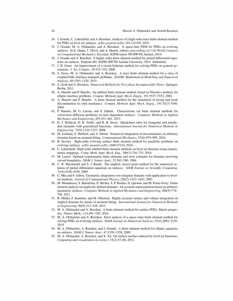
44 Maxim A. Olshanskii and Arnold Reusken
34. J. Grande, C. Lehrenfeld, and A. Reusken. Analysis of a high order trace finite element methodfor PDEs on level set surfaces. arXiv preprint arXiv:1611.01100, 2016.
35. J. Grande, M. A. Olshanskii, and A. Reusken. A space-time FEM for PDEs on evolvingsurfaces. In E. Onate, J. Oliver, and A. Huerta, editors, proceedings of 11th World Congresson Computational Mechanics. Eccomas. IGPM report 386 RWTH Aachen, 2014.
36. J. Grande and A. Reusken. A higher order finite element method for partial differential equa-tions on surfaces. Preprint 401, IGPM, RWTH Aachen University, 2014. Submitted.
37. J. B. Greer. An improvement of a recent Eulerian method for solving PDEs on general ge-ometries. J. Sci. Comput., 29:321–352, 2008.
38. S. Gross, M. A. Olshanskii, and A. Reusken. A trace finite element method for a class ofcoupled bulk–interface transport problems. ESAIM: Mathematical Modelling and NumericalAnalysis, 49:1303–1330, 2015.
39. S. Groß and A. Reusken. Numerical Methods for Two-phase Incompressible Flows. Springer,Berlin, 2011.
40. A. Hansbo and P. Hansbo. An unfitted finite element method, based on Nitsche’s method, forelliptic interface problems. Comput. Methods Appl. Mech. Engrg., 191:5537–5552, 2002.
41. A. Hansbo and P. Hansbo. A finite element method for the simulation of strong and weakdiscontinuities in solid mechanics. Comput. Methods Appl. Mech. Engrg., 193:3523–3540,2004.
42. P. Hansbo, M. G. Larson, and S. Zahedi. Characteristic cut finite element methods forconvection–diffusion problems on time dependent surfaces. Computer Methods in AppliedMechanics and Engineering, 293:431–461, 2015.
43. D. J. Holdych, D. R. Noble, and R. B. Secor. Quadrature rules for triangular and tetrahe-dral elements with generalized functions. International Journal for Numerical Methods inEngineering, 73(9):1310–1327, 2008.
44. M. Joulaian, S. Hubrich, and A. Duster. Numerical integration of discontinuities on arbitrarydomains based on moment fitting. Computational Mechanics, 57(6):979–999, 2016.
45. B. Kovacs. High-order evolving surface finite element method for parabolic problems onevolving surfaces. arXiv preprint arXiv:1606.07234, 2016.
46. C. Lehrenfeld. High order unfitted finite element methods on level set domains using isopara-metric mappings. Comp. Meth. Appl. Mech. Eng., 300(1):716–733, 2016.
47. M. Lenoir. Optimal isoparametric finite elements and error estimates for domains involvingcurved boundaries. SIAM J. Numer. Anal., 23:562–580, 1986.
48. C. B. Macdonald and S. J. Ruuth. The implicit closest point method for the numerical so-lution of partial differential equations on surfaces. SIAM Journal on Scientific Computing,31(6):4330–4350, 2009.
49. C. Min and F. Gibou. Geometric integration over irregular domains with application to level-set methods. Journal of Computational Physics, 226(2):1432–1443, 2007.
50. M. Moumnassi, S. Belouettar, E. Bechet, S. P. Bordas, D. Quoirin, and M. Potier-Ferry. Finiteelement analysis on implicitly defined domains: An accurate representation based on arbitraryparametric surfaces. Computer Methods in Applied Mechanics and Engineering, 200(5):774–796, 2011.
51. B. Muller, F. Kummer, and M. Oberlack. Highly accurate surface and volume integration onimplicit domains by means of moment-fitting. International Journal for Numerical Methodsin Engineering, 96(8):512–528, 2013.
52. M. A. Olshanskii and A. Reusken. A finite element method for surface PDEs: Matrix proper-ties. Numer. Math., 114:491–520, 2010.
53. M. A. Olshanskii and A. Reusken. Error analysis of a space–time finite element method forsolving PDEs on evolving surfaces. SIAM Journal on Numerical Analysis, 52(4):2092–2120,2014.
54. M. A. Olshanskii, A. Reusken, and J. Grande. A finite element method for elliptic equationson surfaces. SIAM J. Numer. Anal., 47:3339–3358, 2009.
55. M. A. Olshanskii, A. Reusken, and X. Xu. On surface meshes induced by level set functions.Computing and visualization in science, 15(2):53–60, 2012.

Trace Finite Element Methods for PDEs on Surfaces 45
56. M. A. Olshanskii, A. Reusken, and X. Xu. An Eulerian space–time finite element method fordiffusion problems on evolving surfaces. SIAM J. Numer. Anal., 52:1354–1377, 2014.
57. M. A. Olshanskii, A. Reusken, and X. Xu. A stabilized finite element method for advection-diffusion equations on surfaces. IMA J. of Numer. Anal., 34:732–758, 2014.
58. M. A. Olshanskii and D. Safin. A narrow-band unfitted finite element method for elliptic PDEsposed on surfaces. Mathematics of Computation, 85(300):1549–1570, 2016.
59. M. A. Olshanskii and D. Safin. Numerical integration over implicitly defined domains forhigher order unfitted finite element methods. Lobachevskii Journal of Mathematics, 37:582–596, 2016.
60. M. A. Olshanskii and X. Xu. A trace finite element method for PDEs on evolving surfaces.arXiv preprint arXiv:1610.05831, 2016.
61. A. Petras and S. Ruuth. PDEs on moving surfaces via the closest point method and a modifiedgrid based particle method. Journal of Computational Physics, 312:139–156, 2016.
62. F. Ravera, M. Ferrari, and L. Liggieri. Adsorption and partition of surfactants in liquid-liquidsystems. Advances in Colloid and Interface Science, 88:129–177, 2000.
63. A. Reusken. Analysis of trace finite element methods for surface partial differential equations.IMA Journal of Numerical Analysis, 35(4):1568–1590, 2015.
64. H.-G. Roos, M. Stynes, and L. Tobiska. Numerical Methods for Singularly Perturbed Differ-ential Equations — Convection-Diffusion and Flow Problems, volume 24 of Springer Seriesin Computational Mathematics. Springer-Verlag, Berlin, second edition, 2008.
65. S. J. Ruuth and B. Merriman. A simple embedding method for solving partial differentialequations on surfaces. Journal of Computational Physics, 227(3):1943–1961, 2008.
66. R. Saye. High-order quadrature methods for implicitly defined surfaces and volumes in hy-perrectangles. SIAM Journal on Scientific Computing, 37(2):A993–A1019, 2015.
67. J. A. Sethian. A fast marching level set method for monotonically advancing fronts. Proceed-ings of the National Academy of Sciences, 93(4):1591–1595, 1996.
68. S. Tasoglu, U. Demirci, and M. Muradoglu. The effect of soluble surfactant on the transientmotion of a buoyancy-driven bubble. Physics of fluids, 20:040805–1, 2008.
69. J.-J. Xu, Z. Li, J. Lowengrub, and H. Zhao. A level-set method for interfacial flows withsurfactant. Journal of Computational Physics, 212(2):590–616, 2006.
70. J.-J. Xu and H.-K. Zhao. An Eulerian formulation for solving partial differential equationsalong a moving interface. Journal of Scientific Computing, 19:573–594, 2003.