toxicological review of trichloroethylene appendix c · toxicological review of trichloroethylene...
TRANSCRIPT
EPA/635/R-09/011F www.epa.gov/iris
TOXICOLOGICAL REVIEW
OF
TRICHLOROETHYLENE
APPENDIX C
(CAS No. 79-01-6)
In Support of Summary Information on the Integrated Risk Information System (IRIS)
September 2011
C-1
C. META-ANALYSIS OF CANCER RESULTS FROM
EPIDEMIOLOGICAL STUDIES
C.1. METHODOLOGY
An initial review of the epidemiological studies indicated some evidence for associations
between TCE exposure and NHL and cancers of the kidney and liver (see Section 4.1). To
investigate further these possible associations, we performed meta-analyses of the
epidemiological study results for these three cancer types. There was suggestive evidence for
some other cancer types, as well; however, fewer TCE studies reported RR estimates for these
other site-specific cancers, and meta-analysis was not attempted for these cancer types (see
Section 4.1). In addition, at the request of our Science Advisory Board (SAB, 2011), we
conducted a meta-analysis of lung cancer in the TCE cohort studies to address the issue of
smoking as a possible confounder in the kidney cancer studies (see Section 4.4.2.3).
Meta-analysis provides a systematic way to combine study results for a given effect
across multiple (sufficiently similar) studies. The resulting summary (weighted average)
estimate is a quantitatively objective way of reflecting results from multiple studies, rather than
relying on a single study, for instance. Combining the results of smaller studies to obtain a
summary estimate also increases the statistical power to observe an effect, if one exists.
Furthermore, meta-analyses typically are accompanied by other analyses of the epidemiological
studies, including analyses of publication bias and investigations of possible factors responsible
for any heterogeneity across studies.
Given the diverse nature of the epidemiological studies for TCE, random-effects models
were used for the primary analyses, and fixed-effect analyses were conducted for comparison.
Both approaches combine study results (in this case, RR estimates) weighted by the inverse
variance; however, they differ in their underlying assumptions about what the study results
represent and how the variances are calculated. For a random-effects model, it is assumed that
there is true heterogeneity across studies and that both between-study and within-study
components of variation need to be taken into account; this was done using the methodology of
DerSimonian and Laird (1986). For a fixed-effect model, it is assumed that the studies are all
essentially measuring the same thing and all of the variance is within-study variance; thus, for
the fixed-effect model, the RR estimate from each study is simply weighted by the inverse of the
(within-study) variance of the estimate.
Studies for the meta-analyses were selected as described in Appendix B, Section B.2.9.
Because each of the cancer types being evaluated is considered rare in the populations being
studied (all have lifetime risks <10%, and all but lung cancer have lifetime risks <3%), the
different measures of RR (e.g., ORs, risk ratios, and rate ratios) are good approximations of each
C-2
other (Rothman and Greenland, 1998) and are included together as RR estimates in the meta-
analyses. (In addition, the meta-analyses of lung cancer and liver cancer comprised only cohort
studies and, thus, no ORs were included in those analyses.) The general approach for selecting
RR estimates was to select the reported RR estimate that best reflected an RR for TCE exposure
vs. no TCE exposure (overall effect). When multiple estimates were available for the same study
based on different subcohorts with different inclusion criteria, the preference for overall
exposure was to select the RR estimate that represented the largest population in the study, while
trying to minimize the likelihood of TCE exposure misclassification. A subcohort with more
restrictive inclusion criteria was selected if the basis was to reduce exposure misclassification
(e.g., including only subjects with more probable TCE exposure), but not if the basis was to
reflect subjects with greater exposure (e.g., routine vs. any exposure).
When available, RR estimates from internal analyses were selected over standardized
incidence or mortality ratios (SIRs, SMRs) and adjusted RR estimates were generally selected
over crude estimates. Incidence estimates would normally be preferred to mortality estimates;
however, for the two studies providing both incidence and mortality results, incidence
ascertainment was for a substantially shorter period of time than mortality follow-up, so the
endpoint with the greater number of cases was used to reflect the results that had better case
ascertainment. Furthermore, RR estimates based on exposure estimates that discounted an
appropriate lag time prior to disease onset were typically preferred over estimates based on
unlagged exposures, although few studies reported lagged results.
For separate analyses, an RR estimate for the highest exposure group was selected from
studies that presented results for different exposure groups. Exposure groups based on some
measure of cumulative exposure were preferred, if available; however, duration was often the
sole exposure metric used.
Sensitivity analyses were generally done to investigate the impact of alternate selection
choices, as well as to estimate the impact of study findings that were not reported. Specific
selection choices are described in the following subsections detailing the actual analyses.
The meta-analysis calculations are based on (natural) logarithm-transformed values.
Thus, each RR estimate was transformed to its natural logarithm (referred to here as ―log RR,‖
the conventional terminology in epidemiology), and either an estimate of the SE of the log RR
was obtained, from which to estimate the variance for the weights, or an estimate of the variance
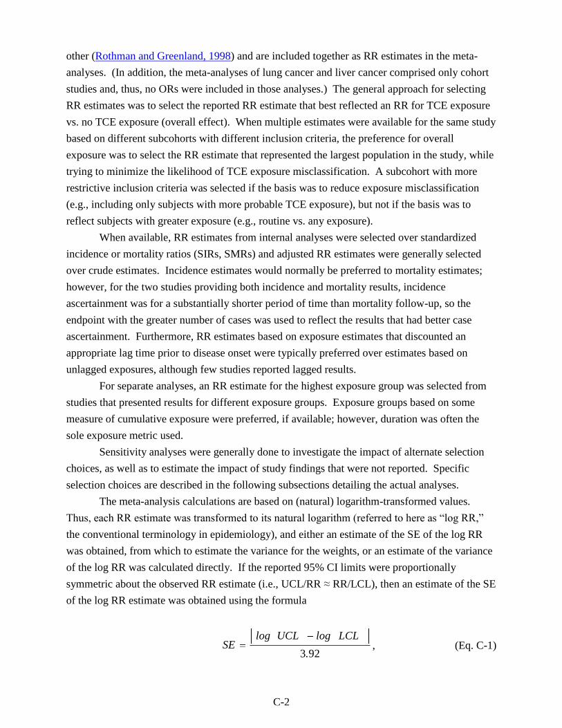
of the log RR was calculated directly. If the reported 95% CI limits were proportionally
symmetric about the observed RR estimate (i.e., UCL/RR ≈ RR/LCL), then an estimate of the SE
of the log RR estimate was obtained using the formula
3 92
log UCL log LCLSE
., (Eq. C-1)
C-3
where UCL is the upper confidence limit and LCL is the lower confidence limit (for 90% CIs,
the divisor is 3.29) (Rothman and Greenland, 1998). In all of the TCE cohort studies reporting
SMRs or SIRs as the overall RR estimates, reported CIs were calculated assuming the number of
deaths (or cases) is approximately Poisson distributed. In such cases, the CIs are not
proportionally symmetric about the RR estimate (unless the number of deaths is fairly large), and
the SE of the log RR estimate was estimated as the inverse of the square root of the observed
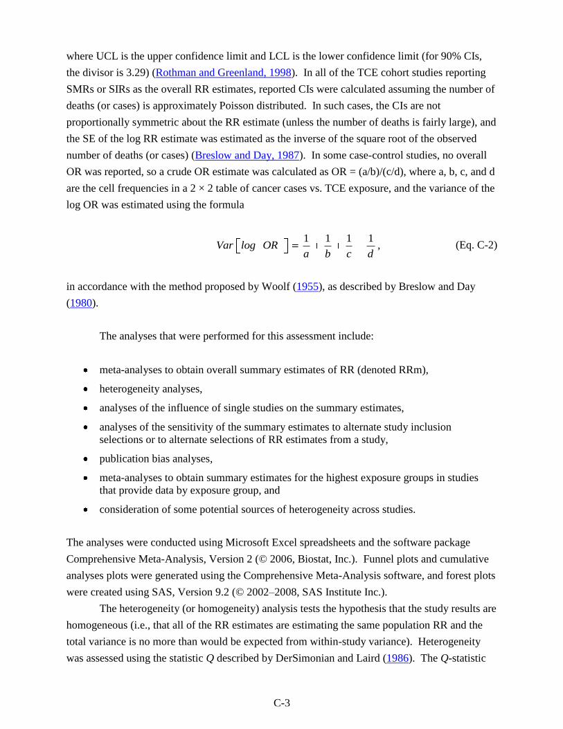
number of deaths (or cases) (Breslow and Day, 1987). In some case-control studies, no overall
OR was reported, so a crude OR estimate was calculated as OR = (a/b)/(c/d), where a, b, c, and d
are the cell frequencies in a 2 × 2 table of cancer cases vs. TCE exposure, and the variance of the
log OR was estimated using the formula
1 1 1 1
Var log OR ,a b c d
(Eq. C-2)
in accordance with the method proposed by Woolf (1955), as described by Breslow and Day
(1980).
The analyses that were performed for this assessment include:
meta-analyses to obtain overall summary estimates of RR (denoted RRm),
heterogeneity analyses,
analyses of the influence of single studies on the summary estimates,
analyses of the sensitivity of the summary estimates to alternate study inclusion
selections or to alternate selections of RR estimates from a study,
publication bias analyses,
meta-analyses to obtain summary estimates for the highest exposure groups in studies
that provide data by exposure group, and
consideration of some potential sources of heterogeneity across studies.
The analyses were conducted using Microsoft Excel spreadsheets and the software package
Comprehensive Meta-Analysis, Version 2 (© 2006, Biostat, Inc.). Funnel plots and cumulative
analyses plots were generated using the Comprehensive Meta-Analysis software, and forest plots
were created using SAS, Version 9.2 (© 2002–2008, SAS Institute Inc.).
The heterogeneity (or homogeneity) analysis tests the hypothesis that the study results are
homogeneous (i.e., that all of the RR estimates are estimating the same population RR and the
total variance is no more than would be expected from within-study variance). Heterogeneity
was assessed using the statistic Q described by DerSimonian and Laird (1986). The Q-statistic
C-4
represents the sum of the weighted squared differences between the summary RR estimate
(obtained under the null hypothesis [i.e., using a fixed-effect model]) and the RR estimate from
each study, and, under the null hypothesis, Q approximately follows a χ2 distribution with
degrees of freedom equal to the number of studies minus one. However, this test can be under-
powered when the number of studies is small, and it is only a significance test (i.e., it is not very
informative about the extent of any heterogeneity). Therefore, the I2 value (Higgins et al., 2003)
was also considered. I2 = 100% × (Q – df)/Q, where Q is the Q-statistic and df is the degrees of
freedom, as described above. This value estimates the percentage of variation that is due to
study heterogeneity. Typically, I2 values of 25, 50, and 75% are considered low, moderate, and
high amounts of heterogeneity, respectively. For a negative value of (Q – df), I2 is set to 0%,
indicating no observable heterogeneity.
Subgroup analyses were sometimes conducted to examine whether or not the combined
RR estimate varied significantly between different types of studies (e.g., case-control vs. cohort
studies). In such subgroup analyses of categorical variables (e.g., study design), ANOVA was
used to determine if there was significant heterogeneity between the subgroups. Applying
ANOVA to meta-analyses with two subgroups (df = 1), Qbetween subgroups = Qoverall – (Qsubgroup1 +
Qsubgroup2) = z-value2, where Qoverall is the Q-statistic calculated across all of the studies and
Qsubgroup1 and Qsubgroup2 are the Q-statistics calculated within each subgroup.
Publication bias is a systematic error that occurs if statistically significant studies are
more likely to be submitted and published than nonsignificant studies. Studies are more likely to
be statistically significant if they have large effect sizes (in this case, RR estimates); thus, an
upward bias would result in a meta-analysis if the available published studies have higher effect
sizes than the full set of studies that were actually conducted. One feature of publication bias is
that smaller studies tend to have larger effect sizes than larger studies, since smaller studies need
larger effect sizes in order to be statistically significant. Thus, many of the techniques used to
analyze publication bias examine whether or not effect size is associated with study size.
Methods used to investigate potential publication bias for this assessment included funnel plots,
which plot effect size vs. study size (actually, SE vs. log RR here); the ―trim and fill‖ procedure
of Duval and Tweedie (2000), which imputes the ―missing‖ studies in a funnel plot (i.e., the
studies needed to counterbalance an asymmetry in the funnel plot resulting from an ostensible
publication bias) and recalculates a summary effect size with these studies present; forest plots
(arrays of RRs and CIs by study) sorted by precision (i.e., SE) to see if effect size shifts with
study size; Begg and Mazumdar rank correlation test (Begg and Mazumdar, 1994), which
examines the correlation between effect size estimates and their variances after standardizing the
effect sizes to stabilize the variances; Egger‘s linear regression test (Egger et al., 1997), which
tests the significance of the bias reflected in the intercept of a regression of effect size/SE on
1/SE; and cumulative meta-analyses after sorting by precision to assess the impact on the
summary effect size estimate of progressively adding the smaller studies.
C-5
C.2. META-ANALYSIS FOR NHL
C.2.1. Overall Effect of TCE Exposure
C.2.1.1. Selection of RR Estimates
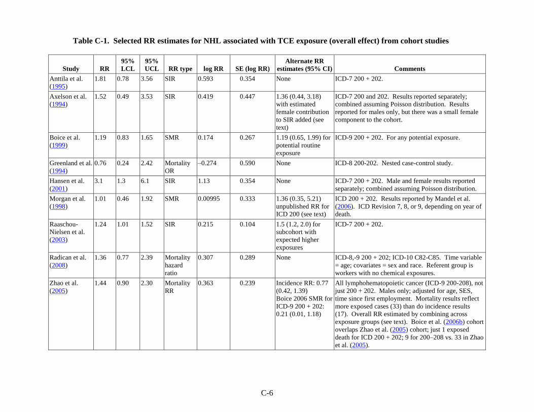
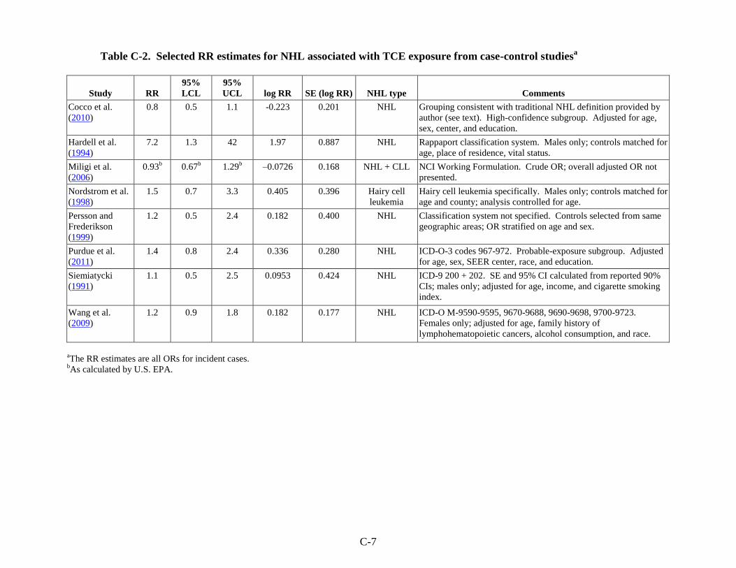
The selected RR estimates for NHL associated with TCE exposure from the selected
epidemiological studies are presented in Table C-1 for cohort studies and in Table C-2 for case-
control studies. Some of the more recent case-control studies classified NHLs along the lines of
the recent World Health Organization/Revised European-American Classification of Lymphoid
Neoplasms (WHO/REAL) classification system (Harris et al., 2000), which recognizes
lymphocytic leukemias and multiple myelomas (plasma cell myelomas) as (non-Hodgkin)
lymphomas; however, most of the available TCE studies reported NHL results according to the
International Classification of Diseases (ICD), Revisions 7, 8, and 9, using a traditional
definition of NHL that excluded lymphocytic leukemias and multiple myelomas and focused on
ICD-7, -8, -9 codes 200 + 202. For consistency of endpoint in the NHL meta-analyses, RR
estimates for ICD 200 + 202 were selected, wherever possible; otherwise, estimates for the
classification(s) best approximating this traditional definition of NHL were selected. In addition,
many of the studies provided RR estimates only for males and females combined, and we are not
aware of any basis for a sex difference in the effects of TCE on NHL risk; thus, wherever
possible, RR estimates for males and females combined were used. The only study of much size
(in terms of number of NHL cancer cases) that provided results separately by sex was Raaschou-
Nielsen et al. (2003). This study reports an insignificantly higher SIR for females (1.4, 95% CI:
0.73, 2.34) than for males (1.2, 95% CI: 0.98, 1.52).
C-6
Table C-1. Selected RR estimates for NHL associated with TCE exposure (overall effect) from cohort studies
Study RR
95%
LCL
95%
UCL RR type log RR SE (log RR)
Alternate RR
estimates (95% CI) Comments
Anttila et al.
(1995)
1.81 0.78 3.56 SIR 0.593 0.354 None ICD-7 200 + 202.
Axelson et al.
(1994)
1.52 0.49 3.53 SIR 0.419 0.447 1.36 (0.44, 3.18)
with estimated
female contribution
to SIR added (see
text)
ICD-7 200 and 202. Results reported separately;
combined assuming Poisson distribution. Results
reported for males only, but there was a small female
component to the cohort.
Boice et al.
(1999)
1.19 0.83 1.65 SMR 0.174 0.267 1.19 (0.65, 1.99) for
potential routine
exposure
ICD-9 200 + 202. For any potential exposure.
Greenland et al.
(1994)
0.76 0.24 2.42 Mortality
OR
–0.274 0.590 None ICD-8 200-202. Nested case-control study.
Hansen et al.
(2001)
3.1 1.3 6.1 SIR 1.13 0.354 None ICD-7 200 + 202. Male and female results reported
separately; combined assuming Poisson distribution.
Morgan et al.
(1998)
1.01 0.46 1.92 SMR 0.00995 0.333 1.36 (0.35, 5.21)
unpublished RR for
ICD 200 (see text)
ICD 200 + 202. Results reported by Mandel et al.
(2006). ICD Revision 7, 8, or 9, depending on year of
death.
Raaschou-
Nielsen et al.
(2003)
1.24 1.01 1.52 SIR 0.215 0.104 1.5 (1.2, 2.0) for
subcohort with
expected higher
exposures
ICD-7 200 + 202.
Radican et al.
(2008)
1.36 0.77 2.39 Mortality
hazard
ratio
0.307 0.289 None ICD-8,-9 200 + 202; ICD-10 C82-C85. Time variable
= age; covariates = sex and race. Referent group is
workers with no chemical exposures.
Zhao et al.
(2005)
1.44 0.90 2.30 Mortality
RR
0.363 0.239 Incidence RR: 0.77
(0.42, 1.39)
Boice 2006 SMR for
ICD-9 200 + 202:
0.21 (0.01, 1.18)
All lymphohematopoietic cancer (ICD-9 200-208), not
just 200 + 202. Males only; adjusted for age, SES,
time since first employment. Mortality results reflect
more exposed cases (33) than do incidence results
(17). Overall RR estimated by combining across
exposure groups (see text). Boice et al. (2006b) cohort
overlaps Zhao et al. (2005) cohort; just 1 exposed
death for ICD 200 + 202; 9 for 200–208 vs. 33 in Zhao
et al. (2005).
C-7
Table C-2. Selected RR estimates for NHL associated with TCE exposure from case-control studiesa
Study RR
95%
LCL
95%
UCL log RR SE (log RR) NHL type Comments
Cocco et al.
(2010)
0.8 0.5 1.1 -0.223 0.201 NHL Grouping consistent with traditional NHL definition provided by
author (see text). High-confidence subgroup. Adjusted for age,
sex, center, and education.
Hardell et al.
(1994)
7.2 1.3 42 1.97 0.887 NHL Rappaport classification system. Males only; controls matched for
age, place of residence, vital status.
Miligi et al.
(2006)
0.93b
0.67b 1.29
b –0.0726 0.168 NHL + CLL NCI Working Formulation. Crude OR; overall adjusted OR not
presented.
Nordstrom et al.
(1998)
1.5 0.7 3.3 0.405 0.396 Hairy cell
leukemia
Hairy cell leukemia specifically. Males only; controls matched for
age and county; analysis controlled for age.
Persson and
Frederikson
(1999)
1.2 0.5 2.4 0.182 0.400 NHL Classification system not specified. Controls selected from same
geographic areas; OR stratified on age and sex.
Purdue et al.
(2011)
1.4 0.8 2.4 0.336 0.280 NHL ICD-O-3 codes 967-972. Probable-exposure subgroup. Adjusted
for age, sex, SEER center, race, and education.
Siemiatycki
(1991)
1.1 0.5 2.5 0.0953 0.424 NHL ICD-9 200 + 202. SE and 95% CI calculated from reported 90%
CIs; males only; adjusted for age, income, and cigarette smoking
index.
Wang et al.
(2009)
1.2 0.9 1.8 0.182 0.177 NHL ICD-O M-9590-9595, 9670-9688, 9690-9698, 9700-9723.
Females only; adjusted for age, family history of
lymphohematopoietic cancers, alcohol consumption, and race.
aThe RR estimates are all ORs for incident cases.
bAs calculated by U.S. EPA.
C-8
Most of the selections in Tables C-1 and C-2 should be self-evident, but some are
discussed in more detail here, in the order the studies are presented in the tables. For Axelson et
al. (1994), in which a small subcohort of females was studied but only results for the larger male
subcohort were reported, the reported male-only results were used in the primary analysis;
however, an attempt was made to estimate the female contribution to an overall RR estimate for
both sexes and its impact on the meta-analysis. Axelson et al. (1994) reported that there were no
cases of NHL observed in females, but the expected number was not presented. To estimate the
expected number, the expected number for males was multiplied by the ratio of female-to-male
person-years in the study and by the ratio of female-to-male age-adjusted incidence rates for
NHL.4 The male results and the estimated female contribution were then combined into an RR
estimate for both sexes assuming a Poisson distribution, and this alternate RR estimate for the
Axelson et al. (1994) study was used in a sensitivity analysis.
For Boice et al. (1999), results for ―any potential exposure‖ were selected for the primary
analysis, because this exposure category was considered to best represent overall TCE exposure,
and results for ―potential routine exposure,‖ which was characterized as reflecting workers
assumed to have received more cumulative exposure, were used in a sensitivity analysis.
The Greenland et al. (1994) study is a case-control study nested within a worker cohort,
and we treat it here as a cohort study (see Appendix B, Section B.2.9.1). Greenland et al. (1994)
report results only for all lymphomas, including Hodgkin lymphoma (ICD-8 201).
For Morgan et al. (1998), the reported results did not allow for the combination of
ICD 200 and 202, so the SMR estimate for the combined 200 + 202 grouping was taken from the
meta-analysis paper of Mandel et al. (2006), who included one of the investigators from the
Morgan et al. (1998) study. RR estimates for overall TCE exposure from internal analyses of the
Morgan et al. (1998) cohort data were available from an unpublished report (EHS, 1997) (the
published paper only presented the internal analyses results for exposure subgroups), but only for
ICD 200; from these, the RR estimate from the Cox model that included age and sex was
selected, because those are the variables deemed to be important in the published paper (Morgan
et al., 1998). Although the results from internal analyses are generally preferred, in this case, the
SMR estimate was used in the primary analysis and the internal analysis RR estimate was used in
a sensitivity analysis because the latter estimate represented an appreciably smaller number of
deaths (3, based on ICD 200 only) than the SMR estimate (9, based on ICD 200 + 202).
4Person-years for men and women <79 years were obtained from Axelson et al. (1994): 23516.5 and 3691.5,
respectively. Lifetime age-adjusted incidence rates for NHL for men and women were obtained from the National
Cancer Institute‘s 2000-2004 SEER-17 (Surveillance Epidemiology and End Results from 17 geographical areas)
database (http://seer.cancer.gov/statfacts/html/nhl.html): 23.2/100,000 and 16.3/100,000, respectively. The
calculation for estimating the expected number of cases in females in the cohort assumes that the males and females
have similar TCE exposures and that the relative distributions of age-related incidence risk for the males and
females in the Swedish cohort are adequately represented by the ratios of person-years and U.S. lifetime incidence
rates used in the calculation.
C-9
For Raaschou-Nielsen et al. (2003), results for the full cohort were used for the primary
analysis and results for the subcohort with expected higher exposure levels (≥1-year duration of
employment and year of 1st employment before 1980) were used in a sensitivity analysis.
Raaschou-Nielsen et al. (2003), in their Table 3, also present overall results for NHL with a lag
time of 20 years; however, they use a definition of lag that is different from a lagged exposure in
which exposures prior to disease onset are discounted and it is not clear what their lag time
actually represents5, thus these results were not used in any of the meta-analyses for NHL.
For Radican et al. (2008), the Cox model hazard ratio from the 2000 follow-up was used.
In the Radican et al. (2008) Cox regressions, age was the time variable, and sex and race were
covariates. It should also be noted that the referent group is composed of workers with no
chemical exposures, not just no exposure to TCE.
For Zhao et al. (2005), RR estimates were only reported for ICD-9 200–208 (all
lymphohematopoietic cancers), and not for 200 + 202 alone. Given that other studies have not
reported associations between leukemias and TCE exposure, combining all lymphohematopoietic
cancers would dilute any NHL effect, and the Zhao et al. (2005) results are expected to be an
underestimate of any TCE effect on NHL alone. Another complication with the Zhao et al.
(2005) study is that no results for an overall TCE effect are reported. We were unable to obtain
any overall estimates from the study authors, so, as a best estimate, the results across the
―medium‖ and ―high‖ exposure groups were combined, under assumptions of group
independence, even though the exposure groups are not independent (the ―low‖ exposure group
was the referent group in both cases). Zhao et al. (2005) present RR estimates for both incidence
and mortality; however, the time frame for the incidence accrual is smaller than the time frame
for mortality accrual and fewer exposed incident cases (17) were obtained than deaths (33).
Thus, because better case ascertainment occurred for mortality than for incidence, the mortality
results were used for the primary analysis, and the incidence results were used in a sensitivity
analysis. A sensitivity analysis was also done using results from Boice et al. (2006b) in place of
the Zhao et al. (2005) RR estimate. The cohorts for these studies overlap, so they are not
independent studies and should not be included in the meta-analysis concurrently. Boice et al.
(2006b) report an RR estimate for an overall TCE effect for NHL alone; however, it is based on
far fewer cases (1 death in ICD-9 200 + 202; 9 deaths for 200–208) and is an SMR rather than an
internal analysis RR estimate, so the Zhao et al. (2005) estimates are preferred for the primary
analysis.
For the case-control studies, the main issue was the NHL classifications. Cocco et al.
(2010) present results for NHLs classified according to the WHO/REAL classification system
(i.e., including lymphocytic leukemias and multiple myelomas). For this meta-analysis, we were
able to obtain results for a grouping of lymphomas generally consistent with the traditional
5In their Methods section, Raaschou-Nielsen et al. (2003) define their lag period as the period ―from the date of first
employment to the start of follow-up for cancer‖.
C-10
definition of NHL (T-cell lymphomas and B-cell lymphomas, excluding Hodgkin lymphomas,
CLLs, multiple myelomas, and unspecified lymphomas) from Dr. Cocco (personal
communication from Pierluigi Cocco, University of Cagliari, Italy, to Cheryl Scott, U.S. EPA,
19 March 2011; see Section 4.6.1.2). The results used in the meta-analyses are for the high-
confidence subgroup, which included workers with jobs with a ―certain‖ probability of exposure
and >90% of workers exposed (5.5% of cases).
Hardell et al. (1994) used the Rappaport classification system, which, according to
Weisenburger (1992) is consistent with the traditional definition of NHL.
Miligi et al. (2006) include CLLs in their NHL results, consistent with the current
WHO/REAL classification. Also, Miligi et al. (2006) do not report an overall adjusted RR
estimate, so a crude estimate of the OR was calculated for the two TCE exposure categories
together vs. no TCE exposure.
The Nordstrom et al. (1998) study was a case-control study of hairy cell leukemias, so
only results for hairy cell leukemia were reported. Hairy cell leukemias are a subgroup of NHLs
under current classification systems, but they were not included in the traditional definition of
NHL.
Persson and Frederikson (1999) did not report the classification system used.
According to Schenk et al.(2009), Purdue et al. (2011) used ICD-O-3 codes 967-972,
which are generally consistent with the traditional definition of NHL. The results used in the
meta-analyses are for the probable-exposure subgroup, which includes workers with at least one
job assigned an exposure probability of ≥50% (3.8% of cases).
According to Zhang et al. (2004), Wang et al. (2009) used ICD-O-2 codes M-9590-9595,
9670-9688, 9690-9698, 9700-9723, which are consistent with the traditional definition of NHL
(i.e., ICD-7, -8, -9 codes 200 + 202).
No alternate RR estimates were considered for any of the case-control studies of NHL.
For the Cocco et al. (2010) and Purdue et al. (2011) studies, the RR estimates used are for a
higher confidence subgroup. No overall results for the full studies were presented to use as
alternative estimates. Results for lower confidence subgroups were presented separately, but no
attempt was made to combine the results across confidence groups because these results were not
independent, as they relied on the same referent groups.
An alternate analysis was done including only the studies for which RR estimates for the
traditional definition of NHL were available. In this analysis, Miligi et al. (2006), Nordstrom et
al.(1998), Persson and Frederikson (1999), and Greenland et al. (1994) were omitted and the
Boice et al. (2006b) cohort study was used instead of Zhao et al. (2005).
C.2.1.2. Results of Meta-Analyses
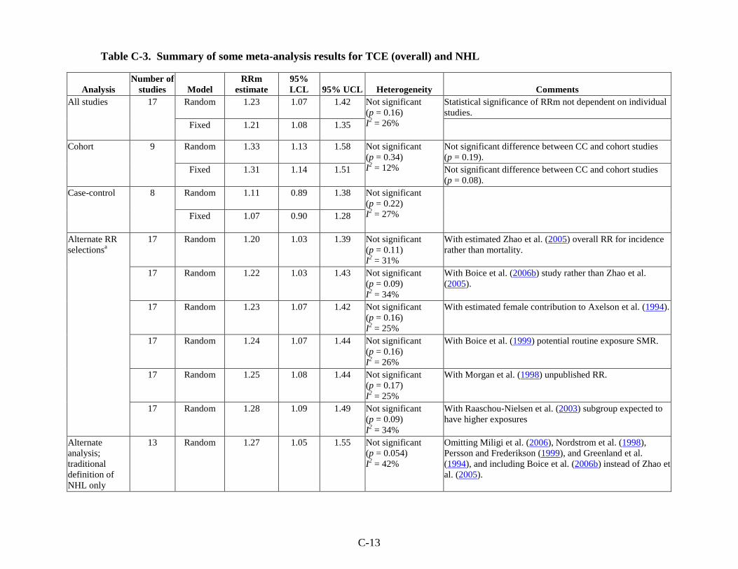
Results from some of the meta-analyses that were conducted on the epidemiological
studies of TCE and NHL are summarized in Table C-3. The summary estimate (RRm) from the
C-11
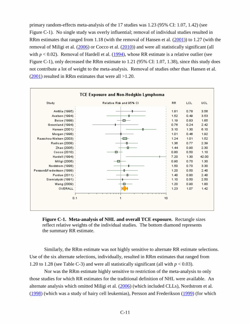
primary random-effects meta-analysis of the 17 studies was 1.23 (95% CI: 1.07, 1.42) (see
Figure C-1). No single study was overly influential; removal of individual studies resulted in
RRm estimates that ranged from 1.18 (with the removal of Hansen et al. (2001)) to 1.27 (with the
removal of Miligi et al. (2006) or Cocco et al. (2010)) and were all statistically significant (all
with p < 0.02). Removal of Hardell et al. (1994), whose RR estimate is a relative outlier (see
Figure C-1), only decreased the RRm estimate to 1.21 (95% CI: 1.07, 1.38), since this study does
not contribute a lot of weight to the meta-analysis. Removal of studies other than Hansen et al.
(2001) resulted in RRm estimates that were all >1.20.
Figure C-1. Meta-analysis of NHL and overall TCE exposure. Rectangle sizes
reflect relative weights of the individual studies. The bottom diamond represents
the summary RR estimate.
Similarly, the RRm estimate was not highly sensitive to alternate RR estimate selections.
Use of the six alternate selections, individually, resulted in RRm estimates that ranged from
1.20 to 1.28 (see Table C-3) and were all statistically significant (all with p < 0.03).
Nor was the RRm estimate highly sensitive to restriction of the meta-analysis to only
those studies for which RR estimates for the traditional definition of NHL were available. An
alternate analysis which omitted Miligi et al. (2006) (which included CLLs), Nordstrom et al.
(1998) (which was a study of hairy cell leukemias), Persson and Frederikson (1999) (for which
C-12
the classification system not specified), and Greenland et al. (1994) (which included Hodgkin
lymphomas) and which included Boice et al. (2006b) instead of Zhao et al. (2005) (which
included all lymphohematopoietic cancers) yielded an RRm estimate of 1.27 (95% CI: 1.05,
1.55).
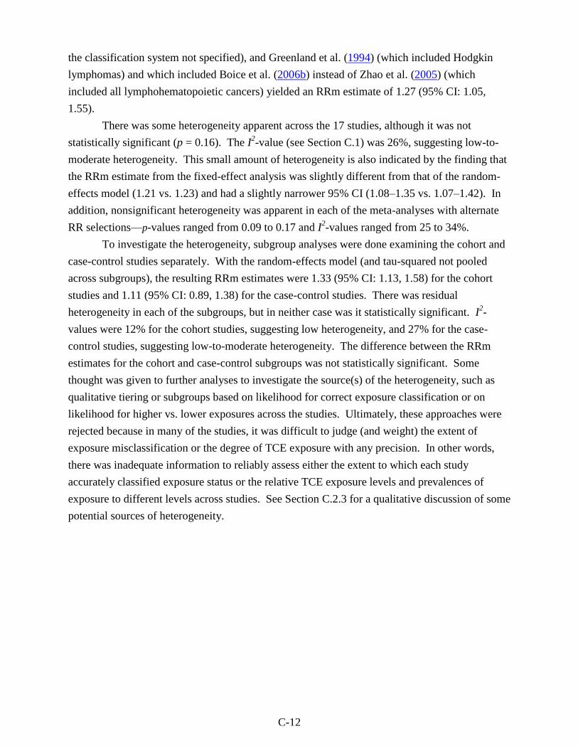
There was some heterogeneity apparent across the 17 studies, although it was not
statistically significant (p = 0.16). The I2-value (see Section C.1) was 26%, suggesting low-to-
moderate heterogeneity. This small amount of heterogeneity is also indicated by the finding that
the RRm estimate from the fixed-effect analysis was slightly different from that of the random-
effects model (1.21 vs. 1.23) and had a slightly narrower 95% CI (1.08–1.35 vs. 1.07–1.42). In
addition, nonsignificant heterogeneity was apparent in each of the meta-analyses with alternate
RR selections—p-values ranged from 0.09 to 0.17 and I2-values ranged from 25 to 34%.
To investigate the heterogeneity, subgroup analyses were done examining the cohort and
case-control studies separately. With the random-effects model (and tau-squared not pooled
across subgroups), the resulting RRm estimates were 1.33 (95% CI: 1.13, 1.58) for the cohort
studies and 1.11 (95% CI: 0.89, 1.38) for the case-control studies. There was residual
heterogeneity in each of the subgroups, but in neither case was it statistically significant. I2-
values were 12% for the cohort studies, suggesting low heterogeneity, and 27% for the case-
control studies, suggesting low-to-moderate heterogeneity. The difference between the RRm
estimates for the cohort and case-control subgroups was not statistically significant. Some
thought was given to further analyses to investigate the source(s) of the heterogeneity, such as
qualitative tiering or subgroups based on likelihood for correct exposure classification or on
likelihood for higher vs. lower exposures across the studies. Ultimately, these approaches were
rejected because in many of the studies, it was difficult to judge (and weight) the extent of
exposure misclassification or the degree of TCE exposure with any precision. In other words,
there was inadequate information to reliably assess either the extent to which each study
accurately classified exposure status or the relative TCE exposure levels and prevalences of
exposure to different levels across studies. See Section C.2.3 for a qualitative discussion of some
potential sources of heterogeneity.
C-13
Table C-3. Summary of some meta-analysis results for TCE (overall) and NHL
Analysis
Number of
studies Model
RRm
estimate
95%
LCL 95% UCL Heterogeneity Comments
All studies
17 Random 1.23 1.07 1.42 Not significant
(p = 0.16)
I2 = 26%
Statistical significance of RRm not dependent on individual
studies.
Fixed 1.21 1.08 1.35
Cohort
9 Random 1.33 1.13 1.58 Not significant
(p = 0.34)
I2 = 12%
Not significant difference between CC and cohort studies
(p = 0.19).
Fixed 1.31 1.14 1.51 Not significant difference between CC and cohort studies
(p = 0.08).
Case-control
8 Random
1.11 0.89 1.38 Not significant
(p = 0.22)
I2 = 27%
Fixed
1.07 0.90 1.28
Alternate RR
selectionsa
17 Random 1.20 1.03 1.39 Not significant
(p = 0.11)
I2 = 31%
With estimated Zhao et al. (2005) overall RR for incidence
rather than mortality.
17 Random 1.22 1.03 1.43 Not significant
(p = 0.09)
I2 = 34%
With Boice et al. (2006b) study rather than Zhao et al.
(2005).
17 Random 1.23 1.07 1.42 Not significant
(p = 0.16)
I2 = 25%
With estimated female contribution to Axelson et al. (1994).
17 Random 1.24 1.07 1.44 Not significant
(p = 0.16)
I2 = 26%
With Boice et al. (1999) potential routine exposure SMR.
17 Random 1.25 1.08 1.44 Not significant
(p = 0.17)
I2 = 25%
With Morgan et al. (1998) unpublished RR.
17 Random 1.28 1.09 1.49 Not significant
(p = 0.09)
I2 = 34%
With Raaschou-Nielsen et al. (2003) subgroup expected to
have higher exposures
Alternate
analysis;
traditional
definition of
NHL only
13 Random 1.27 1.05 1.55 Not significant
(p = 0.054)
I2 = 42%
Omitting Miligi et al. (2006), Nordstrom et al. (1998),
Persson and Frederikson (1999), and Greenland et al.
(1994), and including Boice et al. (2006b) instead of Zhao et
al. (2005).
C-14
TableC-3. Summary of some meta-analysis results for TCE (overall) and NHL (continued)
Analysis
Number of
studies Model
RRm
estimate
95%
LCL 95% UCL Heterogeneity Comments
Highest
exposure groups
13 Random 1.43 1.13 1.82 Not significant
(p = 0.30)
I2 = 14%
Statistical significance not dependent on single study.
See Table C-5 for results with alternate RR selections.
Fixed 1.43 1.16 1.75
aChanging the primary analysis by one alternate RR each time; more details on alternate RR estimates in text.
C-15
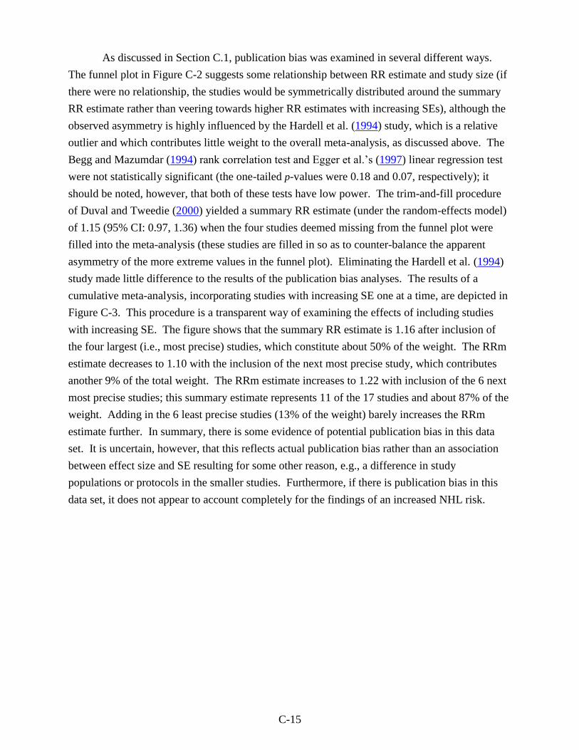
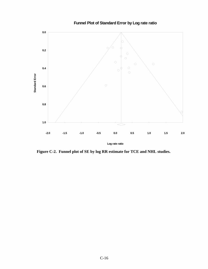
As discussed in Section C.1, publication bias was examined in several different ways.
The funnel plot in Figure C-2 suggests some relationship between RR estimate and study size (if
there were no relationship, the studies would be symmetrically distributed around the summary
RR estimate rather than veering towards higher RR estimates with increasing SEs), although the
observed asymmetry is highly influenced by the Hardell et al. (1994) study, which is a relative
outlier and which contributes little weight to the overall meta-analysis, as discussed above. The
Begg and Mazumdar (1994) rank correlation test and Egger et al.‘s (1997) linear regression test
were not statistically significant (the one-tailed p-values were 0.18 and 0.07, respectively); it
should be noted, however, that both of these tests have low power. The trim-and-fill procedure
of Duval and Tweedie (2000) yielded a summary RR estimate (under the random-effects model)
of 1.15 (95% CI: 0.97, 1.36) when the four studies deemed missing from the funnel plot were
filled into the meta-analysis (these studies are filled in so as to counter-balance the apparent
asymmetry of the more extreme values in the funnel plot). Eliminating the Hardell et al. (1994)
study made little difference to the results of the publication bias analyses. The results of a
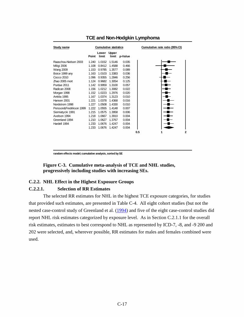
cumulative meta-analysis, incorporating studies with increasing SE one at a time, are depicted in
Figure C-3. This procedure is a transparent way of examining the effects of including studies
with increasing SE. The figure shows that the summary RR estimate is 1.16 after inclusion of
the four largest (i.e., most precise) studies, which constitute about 50% of the weight. The RRm
estimate decreases to 1.10 with the inclusion of the next most precise study, which contributes
another 9% of the total weight. The RRm estimate increases to 1.22 with inclusion of the 6 next
most precise studies; this summary estimate represents 11 of the 17 studies and about 87% of the
weight. Adding in the 6 least precise studies (13% of the weight) barely increases the RRm
estimate further. In summary, there is some evidence of potential publication bias in this data
set. It is uncertain, however, that this reflects actual publication bias rather than an association
between effect size and SE resulting for some other reason, e.g., a difference in study
populations or protocols in the smaller studies. Furthermore, if there is publication bias in this
data set, it does not appear to account completely for the findings of an increased NHL risk.
C-16
Figure C-2. Funnel plot of SE by log RR estimate for TCE and NHL studies.
-2.0 -1.5 -1.0 -0.5 0.0 0.5 1.0 1.5 2.0
0.0
0.2
0.4
0.6
0.8
1.0
Sta
nd
ard
Err
or
Log rate ratio
Funnel Plot of Standard Error by Log rate ratio
C-17
Figure C-3. Cumulative meta-analysis of TCE and NHL studies,
progressively including studies with increasing SEs.
C.2.2. NHL Effect in the Highest Exposure Groups
C.2.2.1. Selection of RR Estimates
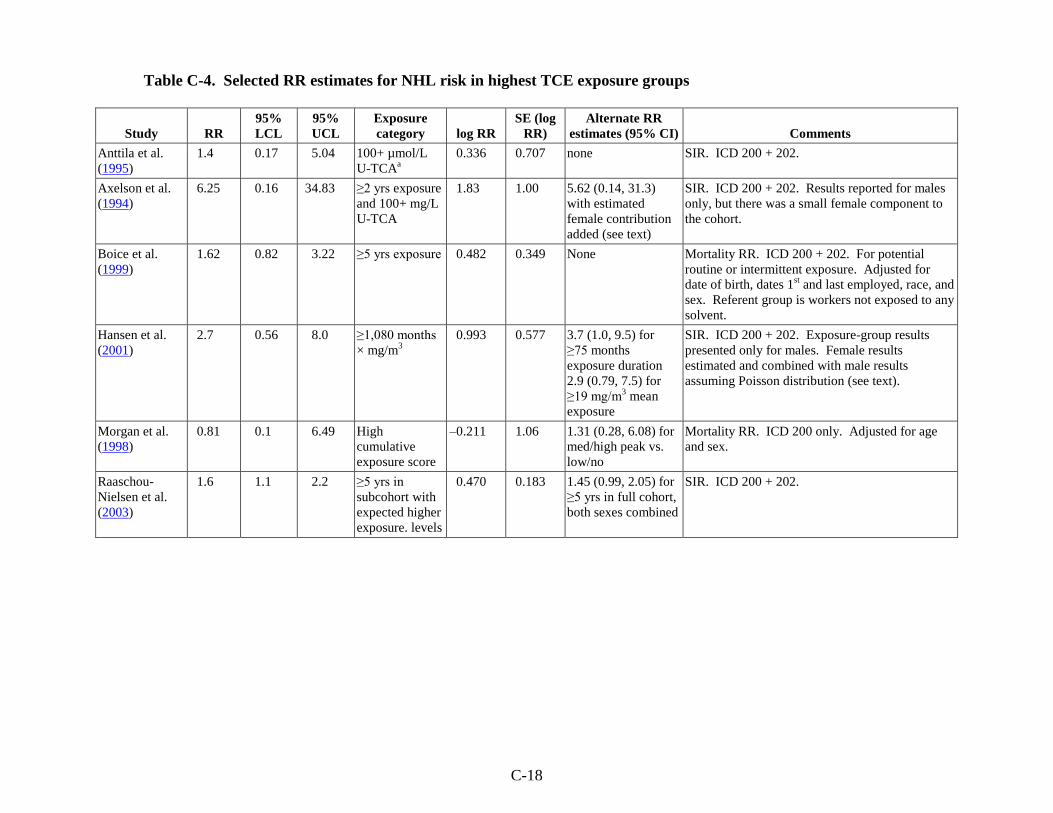
The selected RR estimates for NHL in the highest TCE exposure categories, for studies
that provided such estimates, are presented in Table C-4. All eight cohort studies (but not the
nested case-control study of Greenland et al. (1994) and five of the eight case-control studies did
report NHL risk estimates categorized by exposure level. As in Section C.2.1.1 for the overall
risk estimates, estimates to best correspond to NHL as represented by ICD-7, -8, and -9 200 and
202 were selected, and, wherever possible, RR estimates for males and females combined were
used.
Study name Cumulative statistics Cumulative rate ratio (95% CI)
Lower Upper Point limit limit p-Value
Raaschou-Nielsen 2003 1.240 1.0152 1.5146 0.035
Miligi 2006 1.108 0.8412 1.4588 0.466
Wang 2009 1.153 0.9785 1.3577 0.089
Boice 1999 any 1.163 1.0103 1.3383 0.036
Cocco 2010 1.096 0.9355 1.2846 0.256
Zhao 2005 mort 1.124 0.9682 1.3054 0.125
Purdue 2011 1.142 0.9959 1.3100 0.057
Radican 2008 1.156 1.0212 1.3082 0.022
Morgan 1998 1.152 1.0223 1.2976 0.020
Anttila 1995 1.167 1.0374 1.3123 0.010
Hansen 2001 1.221 1.0378 1.4368 0.016
Nordstrom 1998 1.227 1.0508 1.4330 0.010
Persson&Fredrikson 1999 1.222 1.0555 1.4148 0.007
Siemiatycki 1991 1.215 1.0575 1.3958 0.006
Axelson 1994 1.218 1.0667 1.3910 0.004
Greenland 1994 1.210 1.0627 1.3767 0.004
Hardell 1994 1.233 1.0676 1.4247 0.004
1.233 1.0676 1.4247 0.004
0.5 1 2
TCE and Non-Hodgkin Lymphoma
random effects model; cumulative analysis, sorted by SE
C-18
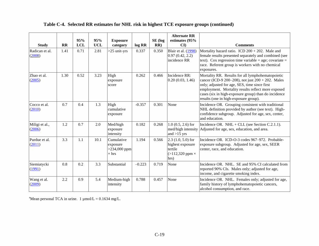
Table C-4. Selected RR estimates for NHL risk in highest TCE exposure groups
Study RR
95%
LCL
95%
UCL
Exposure
category log RR
SE (log
RR)
Alternate RR
estimates (95% CI) Comments
Anttila et al.
(1995)
1.4 0.17 5.04 100+ µmol/L
U-TCAa
0.336 0.707 none SIR. ICD 200 + 202.
Axelson et al.
(1994)
6.25 0.16 34.83 ≥2 yrs exposure
and 100+ mg/L
U-TCA
1.83 1.00 5.62 (0.14, 31.3)
with estimated
female contribution
added (see text)
SIR. ICD 200 + 202. Results reported for males
only, but there was a small female component to
the cohort.
Boice et al.
(1999)
1.62 0.82 3.22 ≥5 yrs exposure 0.482 0.349 None Mortality RR. ICD 200 + 202. For potential
routine or intermittent exposure. Adjusted for
date of birth, dates 1st and last employed, race, and
sex. Referent group is workers not exposed to any
solvent.
Hansen et al.
(2001)
2.7 0.56 8.0 ≥1,080 months
× mg/m3
0.993 0.577 3.7 (1.0, 9.5) for
≥75 months
exposure duration
2.9 (0.79, 7.5) for
≥19 mg/m3 mean
exposure
SIR. ICD 200 + 202. Exposure-group results
presented only for males. Female results
estimated and combined with male results
assuming Poisson distribution (see text).
Morgan et al.
(1998)
0.81 0.1 6.49 High
cumulative
exposure score
–0.211 1.06 1.31 (0.28, 6.08) for
med/high peak vs.
low/no
Mortality RR. ICD 200 only. Adjusted for age
and sex.
Raaschou-
Nielsen et al.
(2003)
1.6 1.1 2.2 ≥5 yrs in
subcohort with
expected higher
exposure. levels
0.470 0.183 1.45 (0.99, 2.05) for
≥5 yrs in full cohort,
both sexes combined
SIR. ICD 200 + 202.
C-19
Table C-4. Selected RR estimates for NHL risk in highest TCE exposure groups (continued)
Study RR
95%
LCL
95%
UCL
Exposure
category log RR
SE (log
RR)
Alternate RR
estimates (95%
CI) Comments
Radican et al.
(2008)
1.41 0.71 2.81 >25 unit-yrs 0.337 0.350 Blair et al. (1998)
0.97 (0.42, 2.2)
incidence RR
Mortality hazard ratio. ICD 200 + 202. Male and
female results presented separately and combined (see
text). Cox regression time variable = age; covariate =
race. Referent group is workers with no chemical
exposures.
Zhao et al.
(2005)
1.30 0.52 3.23 High
exposure
score
0.262 0.466 Incidence RR:
0.20 (0.03, 1.46)
Mortality RR. Results for all lymphohematopoietic
cancer (ICD-9 200–208), not just 200 + 202. Males
only; adjusted for age, SES, time since first
employment. Mortality results reflect more exposed
cases (six in high-exposure group) than do incidence
results (one in high-exposure group).
Cocco et al.
(2010)
0.7 0.4 1.3 High
cumulative
exposure
-0.357 0.301 None Incidence OR. Grouping consistent with traditional
NHL definition provided by author (see text). High-
confidence subgroup. Adjusted for age, sex, center,
and education.
Miligi et al.,
(2006)
1.2 0.7 2.0 Med/high
exposure
intensity
0.182 0.268 1.0 (0.5, 2.6) for
med/high intensity
and >15 yrs
Incidence OR. NHL + CLL (see Section C.2.1.1).
Adjusted for age, sex, education, and area.
Purdue et al.
(2011)
3.3 1.1 10.1 Cumulative
exposure
>234,000 ppm
× hrs
1.194 0.566 2.3 (1.0, 5.0) for
highest exposure
tertile
(>112,320 ppm ×
hrs)
Incidence OR. ICD-O-3 codes 967–972. Probable-
exposure subgroup. Adjusted for age, sex, SEER
center, race, and education.
Siemiatycki
(1991)
0.8 0.2 3.3 Substantial –0.223 0.719 None Incidence OR. NHL. SE and 95% CI calculated from
reported 90% CIs. Males only; adjusted for age,
income, and cigarette smoking index.
Wang et al.
(2009)
2.2 0.9 5.4 Medium-high
intensity
0.788 0.457 None Incidence OR. NHL. Females only; adjusted for age,
family history of lymphohematopoietic cancers,
alcohol consumption, and race.
aMean personal TCA in urine. 1 µmol/L = 0.1634 mg/L.
C-20
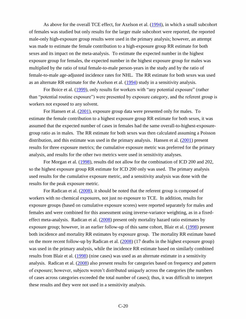
As above for the overall TCE effect, for Axelson et al. (1994), in which a small subcohort
of females was studied but only results for the larger male subcohort were reported, the reported
male-only high-exposure group results were used in the primary analysis; however, an attempt
was made to estimate the female contribution to a high-exposure group RR estimate for both
sexes and its impact on the meta-analysis. To estimate the expected number in the highest
exposure group for females, the expected number in the highest exposure group for males was
multiplied by the ratio of total female-to-male person-years in the study and by the ratio of
female-to-male age-adjusted incidence rates for NHL. The RR estimate for both sexes was used
as an alternate RR estimate for the Axelson et al. (1994) study in a sensitivity analysis.
For Boice et al. (1999), only results for workers with ―any potential exposure‖ (rather
than ―potential routine exposure‖) were presented by exposure category, and the referent group is
workers not exposed to any solvent.
For Hansen et al. (2001), exposure group data were presented only for males. To
estimate the female contribution to a highest exposure group RR estimate for both sexes, it was
assumed that the expected number of cases in females had the same overall-to-highest-exposure-
group ratio as in males. The RR estimate for both sexes was then calculated assuming a Poisson
distribution, and this estimate was used in the primary analysis. Hansen et al. (2001) present
results for three exposure metrics; the cumulative exposure metric was preferred for the primary
analysis, and results for the other two metrics were used in sensitivity analyses.
For Morgan et al. (1998), results did not allow for the combination of ICD 200 and 202,
so the highest exposure group RR estimate for ICD 200 only was used. The primary analysis
used results for the cumulative exposure metric, and a sensitivity analysis was done with the
results for the peak exposure metric.
For Radican et al. (2008), it should be noted that the referent group is composed of
workers with no chemical exposures, not just no exposure to TCE. In addition, results for
exposure groups (based on cumulative exposure scores) were reported separately for males and
females and were combined for this assessment using inverse-variance weighting, as in a fixed-
effect meta-analysis. Radican et al. (2008) present only mortality hazard ratio estimates by
exposure group; however, in an earlier follow-up of this same cohort, Blair et al. (1998) present
both incidence and mortality RR estimates by exposure group. The mortality RR estimate based
on the more recent follow-up by Radican et al. (2008) (17 deaths in the highest exposure group)
was used in the primary analysis, while the incidence RR estimate based on similarly combined
results from Blair et al. (1998) (nine cases) was used as an alternate estimate in a sensitivity
analysis. Radican et al. (2008) also present results for categories based on frequency and pattern
of exposure; however, subjects weren‘t distributed uniquely across the categories (the numbers
of cases across categories exceeded the total number of cases); thus, it was difficult to interpret
these results and they were not used in a sensitivity analysis.
C-21
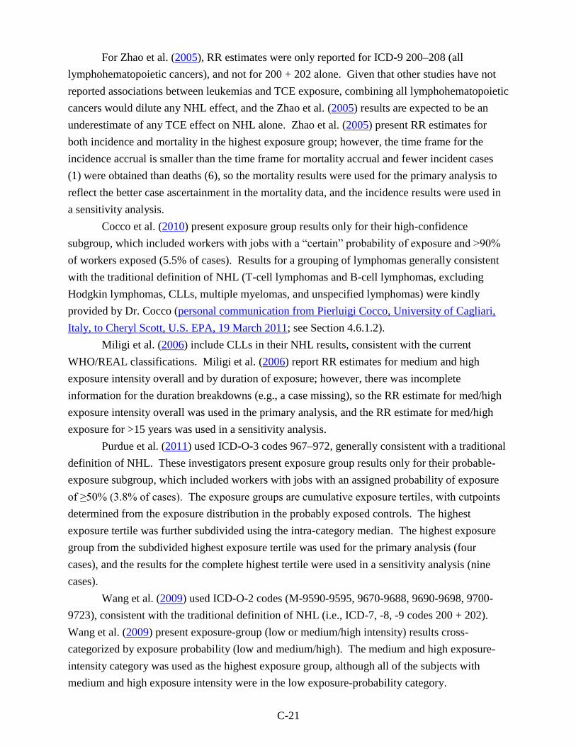
For Zhao et al. (2005), RR estimates were only reported for ICD-9 200–208 (all
lymphohematopoietic cancers), and not for 200 + 202 alone. Given that other studies have not
reported associations between leukemias and TCE exposure, combining all lymphohematopoietic
cancers would dilute any NHL effect, and the Zhao et al. (2005) results are expected to be an
underestimate of any TCE effect on NHL alone. Zhao et al. (2005) present RR estimates for
both incidence and mortality in the highest exposure group; however, the time frame for the
incidence accrual is smaller than the time frame for mortality accrual and fewer incident cases
(1) were obtained than deaths (6), so the mortality results were used for the primary analysis to
reflect the better case ascertainment in the mortality data, and the incidence results were used in
a sensitivity analysis.
Cocco et al. (2010) present exposure group results only for their high-confidence
subgroup, which included workers with jobs with a ―certain‖ probability of exposure and >90%
of workers exposed (5.5% of cases). Results for a grouping of lymphomas generally consistent
with the traditional definition of NHL (T-cell lymphomas and B-cell lymphomas, excluding
Hodgkin lymphomas, CLLs, multiple myelomas, and unspecified lymphomas) were kindly
provided by Dr. Cocco (personal communication from Pierluigi Cocco, University of Cagliari,
Italy, to Cheryl Scott, U.S. EPA, 19 March 2011; see Section 4.6.1.2).
Miligi et al. (2006) include CLLs in their NHL results, consistent with the current
WHO/REAL classifications. Miligi et al. (2006) report RR estimates for medium and high
exposure intensity overall and by duration of exposure; however, there was incomplete
information for the duration breakdowns (e.g., a case missing), so the RR estimate for med/high
exposure intensity overall was used in the primary analysis, and the RR estimate for med/high
exposure for >15 years was used in a sensitivity analysis.
Purdue et al. (2011) used ICD-O-3 codes 967–972, generally consistent with a traditional
definition of NHL. These investigators present exposure group results only for their probable-
exposure subgroup, which included workers with jobs with an assigned probability of exposure
of ≥50% (3.8% of cases). The exposure groups are cumulative exposure tertiles, with cutpoints
determined from the exposure distribution in the probably exposed controls. The highest
exposure tertile was further subdivided using the intra-category median. The highest exposure
group from the subdivided highest exposure tertile was used for the primary analysis (four
cases), and the results for the complete highest tertile were used in a sensitivity analysis (nine
cases).
Wang et al. (2009) used ICD-O-2 codes (M-9590-9595, 9670-9688, 9690-9698, 9700-
9723), consistent with the traditional definition of NHL (i.e., ICD-7, -8, -9 codes 200 + 202).
Wang et al. (2009) present exposure-group (low or medium/high intensity) results cross-
categorized by exposure probability (low and medium/high). The medium and high exposure-
intensity category was used as the highest exposure group, although all of the subjects with
medium and high exposure intensity were in the low exposure-probability category.
C-22
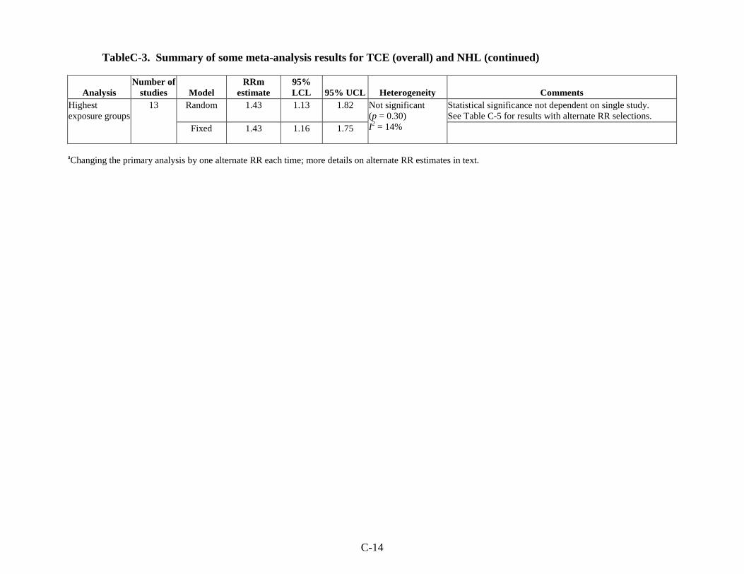
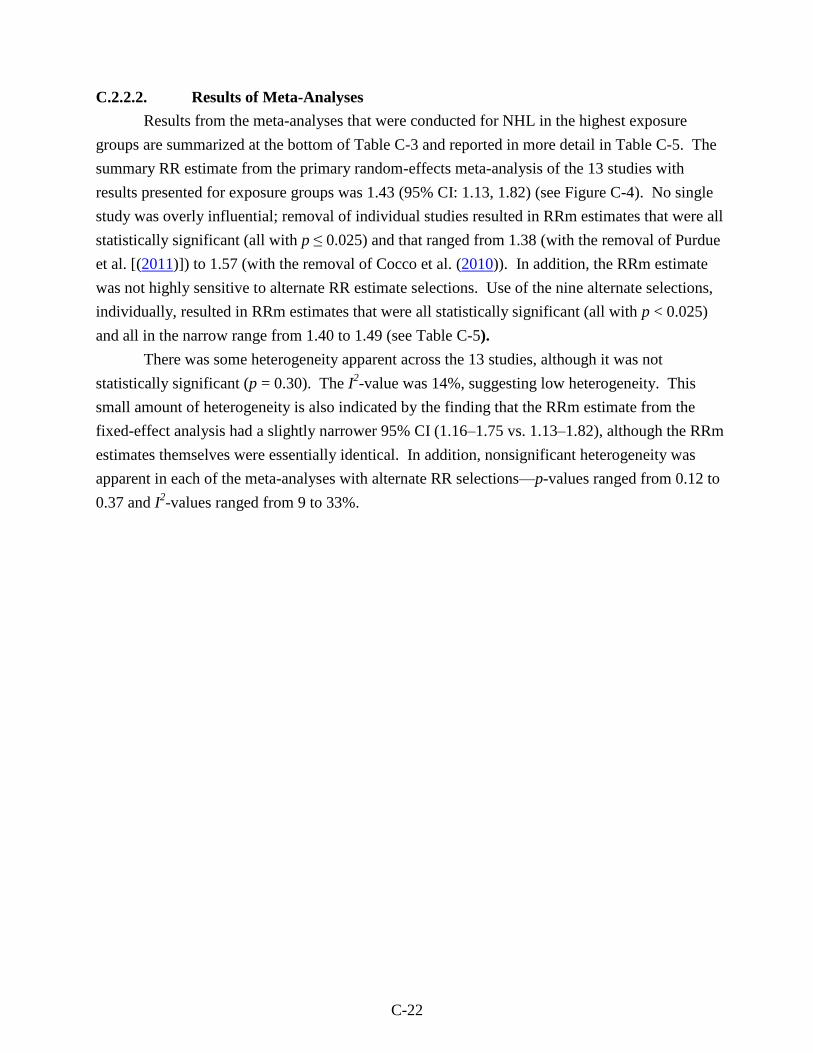
C.2.2.2. Results of Meta-Analyses
Results from the meta-analyses that were conducted for NHL in the highest exposure
groups are summarized at the bottom of Table C-3 and reported in more detail in Table C-5. The
summary RR estimate from the primary random-effects meta-analysis of the 13 studies with
results presented for exposure groups was 1.43 (95% CI: 1.13, 1.82) (see Figure C-4). No single
study was overly influential; removal of individual studies resulted in RRm estimates that were all
statistically significant (all with p ≤ 0.025) and that ranged from 1.38 (with the removal of Purdue
et al. [(2011)]) to 1.57 (with the removal of Cocco et al. (2010)). In addition, the RRm estimate
was not highly sensitive to alternate RR estimate selections. Use of the nine alternate selections,
individually, resulted in RRm estimates that were all statistically significant (all with p < 0.025)
and all in the narrow range from 1.40 to 1.49 (see Table C-5).
There was some heterogeneity apparent across the 13 studies, although it was not
statistically significant (p = 0.30). The I2-value was 14%, suggesting low heterogeneity. This
small amount of heterogeneity is also indicated by the finding that the RRm estimate from the
fixed-effect analysis had a slightly narrower 95% CI (1.16–1.75 vs. 1.13–1.82), although the RRm
estimates themselves were essentially identical. In addition, nonsignificant heterogeneity was
apparent in each of the meta-analyses with alternate RR selections—p-values ranged from 0.12 to
0.37 and I2-values ranged from 9 to 33%.
C-23
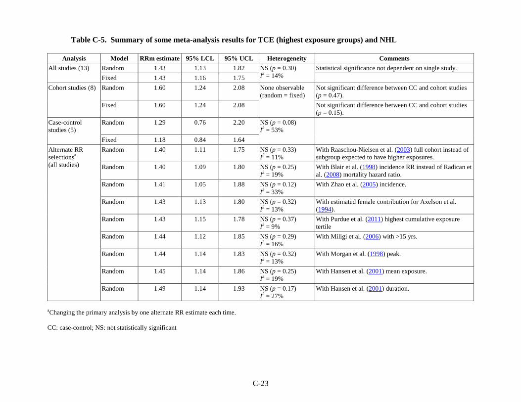
Table C-5. Summary of some meta-analysis results for TCE (highest exposure groups) and NHL
Analysis Model RRm estimate 95% LCL 95% UCL Heterogeneity Comments
All studies (13) Random 1.43 1.13 1.82 NS (p = 0.30)
I2 = 14%
Statistical significance not dependent on single study.
Fixed 1.43 1.16 1.75
Cohort studies (8) Random 1.60 1.24 2.08 None observable
(random = fixed)
Not significant difference between CC and cohort studies
(p = 0.47).
Fixed 1.60 1.24 2.08 Not significant difference between CC and cohort studies
(p = 0.15).
Case-control
studies (5)
Random
1.29 0.76 2.20 NS (p = 0.08)
I2 = 53%
Fixed 1.18 0.84 1.64
Alternate RR
selectionsa
(all studies)
Random 1.40 1.11 1.75 NS (p = 0.33)
I2 = 11%
With Raaschou-Nielsen et al. (2003) full cohort instead of
subgroup expected to have higher exposures.
Random 1.40 1.09 1.80 NS (p = 0.25)
I2 = 19%
With Blair et al. (1998) incidence RR instead of Radican et
al. (2008) mortality hazard ratio.
Random 1.41 1.05 1.88 NS (p = 0.12)
I2 = 33%
With Zhao et al. (2005) incidence.
Random 1.43 1.13 1.80 NS (p = 0.32)
I2 = 13%
With estimated female contribution for Axelson et al.
(1994).
Random 1.43 1.15 1.78 NS (p = 0.37)
I2 = 9%
With Purdue et al. (2011) highest cumulative exposure
tertile
Random 1.44 1.12 1.85 NS (p = 0.29)
I2 = 16%
With Miligi et al. (2006) with >15 yrs.
Random 1.44 1.14 1.83 NS (p = 0.32)
I2 = 13%
With Morgan et al. (1998) peak.
Random 1.45 1.14 1.86 NS (p = 0.25)
I2 = 19%
With Hansen et al. (2001) mean exposure.
Random 1.49 1.14 1.93 NS (p = 0.17)
I2 = 27%
With Hansen et al. (2001) duration.
aChanging the primary analysis by one alternate RR estimate each time.
CC: case-control; NS: not statistically significant
C-24
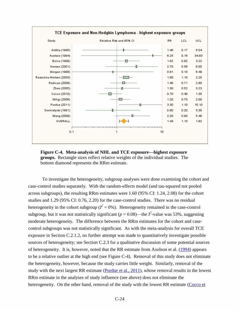
Figure C-4. Meta-analysis of NHL and TCE exposure—highest exposure
groups. Rectangle sizes reflect relative weights of the individual studies. The
bottom diamond represents the RRm estimate.
To investigate the heterogeneity, subgroup analyses were done examining the cohort and
case-control studies separately. With the random-effects model (and tau-squared not pooled
across subgroups), the resulting RRm estimates were 1.60 (95% CI: 1.24, 2.08) for the cohort
studies and 1.29 (95% CI: 0.76, 2.20) for the case-control studies. There was no residual
heterogeneity in the cohort subgroup (I2 = 0%). Heterogeneity remained in the case-control
subgroup, but it was not statistically significant (p = 0.08)—the I2-value was 53%, suggesting
moderate heterogeneity. The difference between the RRm estimates for the cohort and case-
control subgroups was not statistically significant. As with the meta-analysis for overall TCE
exposure in Section C.2.1.2, no further attempt was made to quantitatively investigate possible
sources of heterogeneity; see Section C.2.3 for a qualitative discussion of some potential sources
of heterogeneity. It is, however, noted that the RR estimate from Axelson et al. (1994) appears
to be a relative outlier at the high end (see Figure C-4). Removal of this study does not eliminate
the heterogeneity, however, because the study carries little weight. Similarly, removal of the
study with the next largest RR estimate (Purdue et al., 2011), whose removal results in the lowest
RRm estimate in the analyses of study influence (see above) does not eliminate the
heterogeneity. On the other hand, removal of the study with the lowest RR estimate (Cocco et
C-25
al., 2010), which also has a substantial amount of weight and whose removal results in the
highest RRm estimate in the analyses of study influence (see above), eliminates all of the
heterogeneity. This suggests that the result from Cocco et al. (2010) for the highest exposure
group might be an outlier, but it is unclear what about the study might account for this result
being inordinately low.
C.2.3. Discussion of NHL Meta-Analysis Results
The meta-analyses of the overall effect of TCE exposure on NHL suggest a small,
statistically significant increase in risk. The summary estimate from the primary random-effects
meta-analysis of the 17 studies was 1.23 (95% CI: 1.07, 1.42). This result was not overly
influenced by any single study, nor was it overly sensitive to individual RR estimate selections or
to restricting the analysis to only those studies for which RR estimates based on the traditional
definition of NHL were available, and in all of the influence and sensitivity analyses, the RRm
estimate was statistically significantly increased. Thus, the finding of an increased risk of NHL
associated with TCE exposure, though the increased risk is not large in magnitude, is robust.
There is some evidence of potential publication bias in this data set; however, it is
uncertain that this is actually publication bias rather than an association between SE and effect
size resulting for some other reason (e.g., a difference in study populations or protocols in the
smaller studies). Furthermore, if there is publication bias in this data set, it does not appear to
account completely for the finding of an increased NHL risk. For example, using the trim-and-
fill procedure of Duval and Tweedie (2000) to impute the values from the four ‗missing‘ studies
that would balance the funnel plot yields an RRm estimate of 1.15 (95% CI: 0.97, 1.36).
Although there was some heterogeneity across the 17 studies, it was not statistically
significant (p = 0.16). The I2-value was 26%, suggesting low-to-moderate heterogeneity.
Similarly, when subgroup analyses were done of cohort and case-control studies separately, there
was some observable heterogeneity in each of the subgroups, but it was not statistically
significant in either case. I2-values were 12% for the cohort studies, suggesting low
heterogeneity, and 27% for the case-control studies, suggesting low-to-moderate heterogeneity.
In the subgroup analyses, the increased risk of NHL was strengthened in the cohort study
analysis and nearly eliminated in the case-control study analysis, although the subgroup RRm
estimates were not statistically significantly different. Study design itself is unlikely to be an
underlying cause of heterogeneity and, to the extent that it may explain some of the differences
across studies, is more probably a surrogate for some other difference(s) across studies that may
be associated with study design. Furthermore, other potential sources of heterogeneity may be
masked by the broad study design subgroupings. The true source(s) of heterogeneity across
these studies is an uncertainty. As discussed above, further quantitative investigations of
heterogeneity were ruled out because of database limitations. A qualitative discussion of some
potential sources of heterogeneity follows.
C-26
Study differences in exposure assessment approach, exposure prevalence, average
exposure intensity, and NHL classification are possible sources of heterogeneity. Many studies
included TCE assignment from information on job and task exposures, e.g., a JEM (Radican et
al., 2008; Boice et al., 2006b; Miligi et al., 2006; Zhao et al., 2005; Boice et al., 1999; Morgan et
al., 1998; Siemiatycki, 1991); (Purdue et al., 2011; Cocco et al., 2010; Wang et al., 2009), or
from an exposure biomarker in either breath or urine (Hansen et al., 2001; Anttila et al., 1995;
Axelson et al., 1994). Three case-control studies relied on self-reported exposure to TCE
(Persson and Fredrikson, 1999; Nordström et al., 1998; Hardell et al., 1994). Misclassification is
possible with all exposure assessment approaches. No information is available to judge the
degree of possible misclassification bias associated with a particular exposure assessment
approach; it is quite possible that in some cohort studies, in which past exposure is inferred from
various data sources, exposure misclassification may be as great as in population-based or
hospital-based case-control studies. Approaches based upon JEMs can provide order-of-
magnitude estimates that are useful for distinguishing groups of workers with large differences in
exposure; however, smaller differences usually cannot be reliably distinguished (NRC, 2006).
Biomonitoring can provide information on potential TCE exposure in an individual, but the
biomarkers used aren't necessarily specific for TCE and they reflect only recent exposures.
General population studies have special problems in evaluating exposure, because the
subjects could have worked in any job or setting that is present within the population (NRC,
2006; 't Mannetje et al., 2002; McGuire et al., 1998; Nelson et al., 1994; Copeland et al., 1977).
Low exposure prevalence in the case-control studies may be another source of heterogeneity.
Prevalence of TCE exposure among cases in the case-control studies was low, ranging from 3 in
Siemiatycki (1991) to 13% in Wang et al. (2009). However, prevalence of high TCE exposure in
these case-control studies was even rarer—3% of all cases in Miligi et al. (2006), 2% in Wang et
al. (2009) and Cocco et al. (2010) (high-confidence assessments; personal communication from
Pierluigi Cocco, University of Cagliari, Italy, to Cheryl Scott, U.S. EPA, 19 March 2011; see
Section 4.6.1.2), 1% (with probable exposure) in Purdue et al. (2011), and <1% in Siemiatycki
(1991). Low exposure prevalence may be one of the underlying characteristics differentiating
the case-control and cohort studies and explaining some of the heterogeneity across the studies.
Study differences in NHL groupings and in NHL classification schemes are another
potential source of heterogeneity in the meta-analysis, although restricting the meta-analysis to
only those studies for which RR estimates based on the traditional NHL definition were available
did not eliminate all heterogeneity. All studies included a broad but sometimes slightly different
group of lymphosarcoma, reticulum-cell sarcoma, and other lymphoid tissue neoplasms, with the
exception of the Nordstrom et al. (1998) case-control study, which examined hairy cell leukemia,
now considered a (non-Hodgkin) lymphoma, and the Zhao et al. (2005) cohort study, which
reported only results for all lymphohematopoietic cancers, including nonlymphoid types.
Persson and Fredrikson (1999) do not identify the classification system for defining NHL, and
C-27
Hardell et al. (1994) define NHL using the Rappaport classification system. Miligi et al. (2006)
used the NCI Working Formulation and also considered CLLs as (non-Hodgkin) lymphomas.
Cocco et al. (2010) used the WHO/REAL classification system, which reclassifies lymphocytic
leukemias and NHLs as lymphomas of B-cell or T-cell origin and considers CLLs and multiple
myelomas as (non-Hodgkin) lymphomas; however, results were obtained generally consistent
with the traditional NHL definition from Dr. Cocco, although lymphomas not otherwise
specified were excluded. Wang et al. (2009) defined NHL using ICD-O-2 codes (M-9590-9595,
9670-9688, 9690-9698, 9700-9723), which is consistent with the traditional definition of NHL
(i.e., ICD-7, -8, -9 codes 200 + 202). Purdue et al. (2011) used ICD-O-3 codes 967–972, which
is generally consistent with the traditional definition of NHL, although this grouping doesn‘t
include the malignant lymphomas of unspecified type coded as M-9590-9599. The cohort
studies [except for Zhao et al. (2005)] and the case-control study of Siemiatycki (1991) have
some consistency in coding NHL, with NHL defined as lymphosarcoma and reticulum-cell
sarcoma (ICD code 200) and other lymphoid tissue neoplasms (ICD 202) using the ICD
Revisions 7, 8, or 9. Revisions 7 and 8 are essentially the same with respect to NHL; under
Revision 9, the definition of NHL was broadened to include some neoplasms previously
classified as Hodgkin lymphomas (Banks, 1992).
Thirteen of the 17 studies categorized results by exposure level. Different exposure
metrics were used, and the purpose of combining results across the different highest exposure
groups was not to estimate an RRm associated with some level of exposure, but rather to see the
impacts of combining RR estimates that should be less affected by exposure misclassification.
In other words, the highest exposure category is more likely to represent a greater differential
TCE exposure compared to people in the referent group than the exposure differential for the
overall (typically any vs. none) exposure comparison. Thus, if TCE exposure increases the risk
of NHL, the effects should be more apparent in the highest exposure groups. Indeed, the RRm
estimate from the primary meta-analysis of the highest exposure group results was 1.43 (95% CI:
1.13, 1.82), which is greater than the RRm estimate of 1.23 (95% CI: 1.07, 1.42) from the overall
exposure analysis. The statistical significance of the increased RR estimate for the highest
exposure groups was not dependent on any single study, nor was it sensitive to individual RR
estimate selections. The robustness of this finding lends substantial support to a conclusion that
TCE exposure increases the risk of NHL.
Although there was some heterogeneity apparent across the 13 highest-exposure-group
studies, it was not statistically significant (p = 0.30). The I2-value was 14%, suggesting low
heterogeneity. When subgroup analyses were done examining the cohort and case-control
studies separately, there was no residual heterogeneity in the cohort subgroup (I2 = 0%).
Heterogeneity remained in the case-control subgroup, but it was not statistically significant
(p = 0.08)—the I2-value was 53%, suggesting moderate heterogeneity. In the subgroup analyses,
the increased risk of NHL was strengthened in the cohort study analysis and reduced in the case-
C-28
control study analysis, although the subgroup RRm estimates were not statistically significantly
different. As with the meta-analysis for overall TCE exposure discussed above, no further
attempt was made to quantitatively investigate potential sources of heterogeneity. It is, however,
noted that removal of the Cocco et al. (2010) study, whose removal had the greatest impact in the
analyses of study influence (RRm = 1.57, 95% CI: 1.27, 1.95), eliminates all of the
heterogeneity, suggesting that the RR estimate for the highest exposure group from that study is
a relative outlier.
C.3. META-ANALYSIS FOR KIDNEY CANCER
C.3.1. Overall Effect of TCE Exposure
C.3.1.1. Selection of RR Estimates
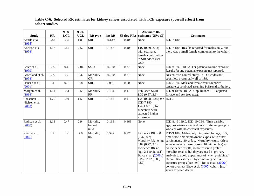
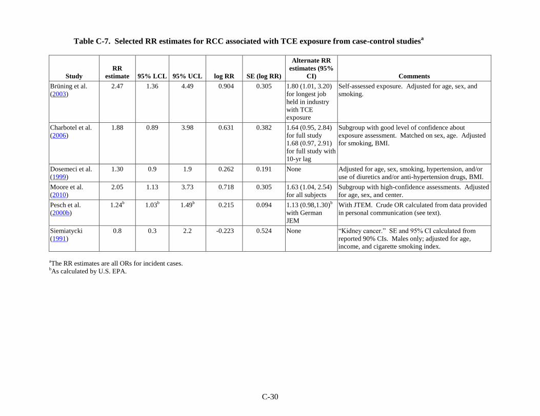
The selected RR estimates for kidney cancer associated with TCE exposure from the
epidemiological studies are presented in Table C-6 for cohort studies and in Table C-7 for case-
control studies. The majority of the cohort studies reported results for all kidney cancers,
including cancers of the renal pelvis and ureter (i.e., ICD-7 180; ICD-8 and -9 189.0–189.2;
ICD-10 C64–C66), whereas the majority of the case-control studies focused on RCC, which
comprises roughly 85% of kidney cancers. Where both all kidney cancer and RCC were
reported, the primary analysis used the results for RCC, because RCC and the other forms of
kidney cancer are very different cancer types and it seemed preferable not to combine them; the
results for all kidney cancers were then used in a sensitivity analysis. The preference for the
RRC results alone is supported by the results in rodent cancer bioassays, where TCE-associated
rat kidney tumors are observed in the renal tubular cells (Section 4.4.5), and in metabolism
studies, where the focus of studies for the GSH conjugation pathway (considered the primary
metabolic pathway for kidney toxicity) is in renal cortical and tubular cells (Sections 3.3.3.3 and
4.4.6).
C-29
Table C-6. Selected RR estimates for kidney cancer associated with TCE exposure (overall effect) from
cohort studies
Study RR
95%
LCL
95%
UCL RR type log RR SE (log RR)
Alternate RR
estimates (95% CI) Comments
Anttila et al.
(1995)
0.87 0.32 1.89 SIR -0.139 0.408 None ICD-7 180.
Axelson et al.
(1994)
1.16 0.42 2.52 SIR 0.148 0.408 1.07 (0.39, 2.33)
with estimated
female contribution
to SIR added (see
text)
ICD-7 180. Results reported for males only, but
there was a small female component to the cohort.
Boice et al.
(1999)
0.99 0.4 2.04 SMR -0.010 0.378 None ICD-9 189.0–189.2. For potential routine exposure.
Results for any potential exposure not reported.
Greenland et al.
(1994)
0.99 0.30 3.32 Mortality
OR
-0.010 0.613 None Nested case-control study. ICD-8 codes not
specified, presumably all of 189.
Hansen et al.
(2001)
1.1 0.3 2.8 SIR 0.095 0.500 None ICD-7 180. Male and female results reported
separately; combined assuming Poisson distribution.
Morgan et al.
(1998)
1.14 0.51 2.58 Mortality
RR
0.134 0.415 Published SMR
1.32 (0.57, 2.6)
ICD-9 189.0–189.2. Unpublished RR, adjusted
for age and sex (see text).
Raaschou-
Nielsen et al.
(2003)
1.20 0.94 1.50 SIR 0.182 0.115 1.20 (0.98, 1.46) for
ICD-7 180
1.4 (1.0, 1.8) for
subcohort with
expected higher
exposures
RCC.
Radican et al.
(2008)
1.18 0.47 2.94 Mortality
hazard
ratio
0.166 0.468 None ICD-8, -9 189.0, ICD-10 C64. Time variable =
age; covariates = sex and race. Referent group is
workers with no chemical exposures.
Zhao et al.
(2005)
1.7 0.38 7.9 Mortality
RR
0.542 0.775 Incidence RR: 2.0
(0.47, 8.2)
Mortality RR no lag:
0.89 (0.22, 3.6)
Incidence RR no
lag : 2.1 (0.56, 8.1)
Boice et al. (2006b)
SMR: 2.22 (0.89,
4.57)
ICD-9 189. Males only. Adjusted for age, SES,
time since first employment, exposure to other
carcinogens. 20-yr lag. Mortality results reflect
same number exposed cases (10 with no lag) as
do incidence results, so no reason to prefer
mortality results, but they are used in primary
analysis to avoid appearance of ―cherry-picking.‖
Overall RR estimated by combining across
exposure groups (see text). Boice et al. (2006b)
cohort overlaps Zhao et al. (2005) cohort; just
seven exposed deaths.
C-30
Table C-7. Selected RR estimates for RCC associated with TCE exposure from case-control studiesa
Study
RR
estimate 95% LCL 95% UCL log RR SE (log RR)
Alternate RR
estimates (95%
CI) Comments
Brüning et al.
(2003)
2.47 1.36 4.49 0.904 0.305 1.80 (1.01, 3.20)
for longest job
held in industry
with TCE
exposure
Self-assessed exposure. Adjusted for age, sex, and
smoking.
Charbotel et al.
(2006)
1.88 0.89 3.98 0.631 0.382 1.64 (0.95, 2.84)
for full study
1.68 (0.97, 2.91)
for full study with
10-yr lag
Subgroup with good level of confidence about
exposure assessment. Matched on sex, age. Adjusted
for smoking, BMI.
Dosemeci et al.
(1999)
1.30 0.9 1.9 0.262 0.191 None Adjusted for age, sex, smoking, hypertension, and/or
use of diuretics and/or anti-hypertension drugs, BMI.
Moore et al.
(2010)
2.05 1.13 3.73 0.718 0.305 1.63 (1.04, 2.54)
for all subjects
Subgroup with high-confidence assessments. Adjusted
for age, sex, and center.
Pesch et al.
(2000b)
1.24b 1.03
b 1.49
b 0.215 0.094 1.13 (0.98,1.30)
b
with German
JEM
With JTEM. Crude OR calculated from data provided
in personal communication (see text).
Siemiatycki
(1991)
0.8 0.3 2.2 -0.223 0.524 None ―Kidney cancer.‖ SE and 95% CI calculated from
reported 90% CIs. Males only; adjusted for age,
income, and cigarette smoking index.
aThe RR estimates are all ORs for incident cases.
bAs calculated by U.S. EPA.
C-31
As for NHL, many of the studies provided RR estimates only for males and females
combined, and we are not aware of any basis for a sex difference in the effects of TCE on kidney
cancer risk; thus, wherever possible, RR estimates for males and females combined were used.
Of the three larger (in terms of number of cases) studies that did provide results separately by
sex, Dosemeci et al. (1999) suggest that there may be a sex difference for TCE exposure and
RCC (OR = 1.04 [95% CI: 0.6, 1.7] in males and 1.96 [95% CI: 1.0, 4.0] in females), while
Raaschou-Nielsen et al. (2003) report the same SIR (1.2) for both sexes and crude ORs
calculated from data from the Pesch et al. (2000b) study (provided in a personal communication
from Beate Pesch, Forschungsinstitut für Arbeitsmedizin [BGFA], to Cheryl Scott, U.S. EPA,
21 February 2008) are 1.28 for males and 1.23 for females. Radican et al. (2008) and Hansen et
al. (2001) also present some results by sex, but both of these studies have too few cases to be
informative about a sex difference for kidney cancer.
Most of the selections in Tables C-6 and C-7 should be self-evident, but some are
discussed in more detail here, in the order the studies are presented in the tables. For Axelson et
al. (1994), in which a small subcohort of females was studied but only results for the larger male
subcohort were reported, the reported male-only results were used in the primary analysis;
however, as for NHL, an attempt was made to estimate the female contribution to an overall RR
estimate for both sexes and its impact on the meta-analysis. Axelson et al. (1994) reported
neither the observed nor the expected number of kidney cancer cases for females. It was
assumed that none was observed. To estimate the expected number, the expected number for
males was multiplied by the ratio of female-to-male person-years in the study and by the ratio of
female-to-male age-adjusted incidence rates for kidney cancer.6 The male results and the
estimated female contribution were then combined into an RR estimate for both sexes assuming
a Poisson distribution, and this alternate RR estimate for the Axelson et al. (1994) study was
used in a sensitivity analysis.
For Boice et al. (1999), only results for ―potential routine exposure‖ were reported for
kidney cancer. Boice et al. (1999) report in general that the SMRs for workers with any potential
exposure ―were similar to those for workers with daily potential exposure.‖
In their published paper, Morgan et al. (1998) present only SMRs for overall TCE
exposure, although the results from internal analyses are presented for exposure subgroups. RR
estimates for overall TCE exposure from the internal analyses of the Morgan et al. (1998) cohort
data were available from an unpublished report (EHS, 1997); from these, the RR estimate from
6Person-years for men and women <79 years were obtained from Axelson et al. (1994): 23516.5 and 3691.5,
respectively. Lifetime age-adjusted incidence rates for cancer of the kidney and renal pelvis for men and women
were obtained from the National Cancer Institute‘s 2000–2004 SEER-17 (Surveillance Epidemiology and End
Results from 17 geographical locations) database (http://seer.cancer.gov/statfacts/html/kidrp.html): 17.8/100,000
and 8.8/100,000, respectively. The calculation for estimating the expected number of cases in females in the cohort
assumes that the males and females have similar TCE exposures and that the relative distributions of age-related
incidence risk for the males and females in the Swedish cohort are adequately represented by the ratios of person-
years and U.S. lifetime incidence rates used in the calculation.
C-32
the Cox model that included age and sex was selected, because those are the variables deemed to
be important in the published paper. The internal analysis RR estimate was preferred for the
primary analysis, and the published SMR result was used in a sensitivity analysis.
Raaschou-Nielsen et al. (2003) reported results for RCC and renal pelvis/ureter
separately. As discussed above, RCC estimates were used in the primary analysis, and the
results for both kidney cancer categories were combined (across sexes as well), assuming a
Poisson distribution, and used in a sensitivity analysis. In another sensitivity analysis, results for
RCC from the subcohort with expected higher exposure levels (≥1-year duration of employment
and year of 1st employment before 1980) were used. Raaschou-Nielsen et al. (2003), in their
Table 3, also present the overall results for RCC and for renal pelvis/ureter cancer with a lag time
of 20 years; however, they use a definition of lag that is different from a lagged exposure in
which exposures prior to disease onset are discounted and it is not clear what their lag time
actually represents7; thus, as for NHL, these results were not used in any of the meta-analyses for
kidney cancer.
For Radican et al. (2008), the Cox model hazard ratio from the 2000 follow-up was used.
In the Radican et al. (2008) Cox regressions, age was the time variable, and sex and race were
covariates. It should also be noted that the referent group is composed of workers with no
chemical exposures, not just no exposure to TCE.
For Zhao et al. (2005), no results for an overall TCE effect are reported. We were unable
to obtain any overall estimates from the study authors, so, as a best estimate, as was done for
NHL, the results across the ―medium‖ and ―high‖ exposure groups were combined, under
assumptions of group independence, even though the exposure groups are not independent (the
―low‖ exposure group was the referent group in both cases). Unlike for NHL, adjustment for
exposure to other carcinogens made a considerable difference, so Zhao et al. (2005) also present
kidney results with this additional adjustment, with and without a 20-year lag. Estimates of RR
with this additional adjustment were selected over those without. In addition, a 20-year lag
seemed reasonable for kidney cancer, so the lagged estimates were preferred to the unlagged;
unlagged estimates were used in sensitivity analyses. Zhao et al. (2005) present RR estimates for
both incidence and mortality. Unlike for NHL, the number of exposed incident cases (10 with no
lag) was identical to the number of deaths, so there was no reason to prefer the mortality results
over the incidence results. (In fact, there were more exposed incident cases [10 vs. 7] after
lagging.) However, the mortality results, which yield a lower RR estimate, were selected for the
primary analysis to avoid any appearance of ―cherry-picking,‖ and incidence RR estimates were
used in sensitivity analyses. A sensitivity analysis was also done using results from Boice et al.
(2006b) in place of the Zhao et al. (2005) RR estimate. The cohorts for these studies overlap, so
they are not independent studies and should not be included in the meta-analysis concurrently.
7In their Methods section, Raaschou-Nielsen et al. (2003) define their lag period as the period ―from the date of first
employment to the start of follow-up for cancer‖.
C-33
Boice et al. (2006b) report results for an overall TCE effect for kidney cancer; however, the
results are SMR estimates rather than internal comparisons and are based on fewer exposed
deaths (7), so either Zhao et al. (2005) estimate is preferred over the Boice et al. (2006b)
estimate.
Regarding the case-control studies, for Brüning et al. (2003), the results based on self-
assessed exposure were preferred because, although TCE exposure was probably under-
ascertained with this measure, there were greater concerns about the result based on the alternate
measure reported—longest-held job in an industry with TCE exposure. Even though this study
was conducted in the Arnsberg region of Germany, an area with high prevalence of exposure to
TCE, the exposure prevalence in both cases (87%) and controls (79%) seemed inordinately high,
and this for not just any job in an industry with TCE exposure, but for the longest-held job.
Furthermore, Table V of Brüning et al. (2003), which presents this result, states that the result is
for longest-held job in industries with TCE or tetrachloroethylene exposure. Additionally, some
of the industries with exposure to TCE presented in Table V have many jobs that would not
entail TCE exposure (e.g., white-collar workers), so the assessment based on industry alone
likely has substantial misclassification. Both of these—inclusion of tetrachloroethylene and
exposure assessment by industry—could result in overstating TCE exposure prevalence. Results
based on the longest-held-job measure were used in a sensitivity analysis.
For Charbotel et al. (2006), results from the analysis that considered ―only job periods
with a good level of confidence for TCE exposure assessment‖ [Table 7 of Charbotel et al.
(2006)] were preferred, as these estimates would presumably be less influenced by exposure
misclassification. Estimates from the full study analysis were used in a sensitivity analysis.
Results for exposure with a 10-year lag are also provided in an unpublished report (Charbotel et
al., 2005); however, lagged results are presented only for the full study and, thus, were similarly
used in a sensitivity analysis.
Likewise, for Moore et al. (2010), results from the analysis that considered high-
confidence assessments only were preferred. Here, the definition of TCE exposure was
restricted to jobs classified as having probable or certain exposure (i.e., at least 40% of workers
with that job were expected to be exposed), so these estimates should be less influenced by
exposure misclassification. The RR estimate from the analysis of all subjects was used in a
sensitivity analysis.
For Pesch et al. (2000b), TCE results were presented for two different exposure
assessments. Estimates using the JTEM approach were preferred because they seemed to
represent a more comprehensive exposure assessment (see Appendix B, Section B.2.4); estimates
based on the JEM approach were used in a sensitivity analysis. Furthermore, results were
presented only by exposure category, with no overall RR estimate reported. Case and control
numbers for the different exposure categories were kindly provided by Dr. Pesch (personal
communication from Beate Pesch, BGFA, to Cheryl Scott, U.S. EPA, 21 February 2008), and we
C-34
calculated crude overall ORs for males and females combined for each exposure assessment
approach.
C.3.1.2. Results of Meta-Analyses
Results from some of the meta-analyses that were conducted on the epidemiological
studies of TCE and kidney cancer are summarized in Table C-8. The summary estimate from the
primary random-effects meta-analysis of the 15 studies was 1.27 (95% CI: 1.13, 1.43) (see
Figure C-5). As shown in Figure C-5, the analysis was dominated by two (contributing over
65% of the weight) or three (about 75% of the weight) large studies. No single study was overly
influential; removal of individual studies resulted in RRm estimates that were all statistically
significant (all with p < 0.005) and that ranged from 1.24 (with the removal of (Brüning et al.,
2003)] to 1.30 (with the removal of Raaschou-Nielsen et al. (2003)).
Similarly, the RRm estimate was not highly sensitive to alternate RR estimate selections.
Use of the 13 alternate selections, individually, resulted in RRm estimates that were all
statistically significant (all with p < 0.0005) and that ranged from 1.21 to 1.32 (see Table C-8).
In fact, as can be seen in Table C-8, all but two of the alternates had negligible impact. The
Zhao et al. (2005), Axelson et al. (1994), Morgan et al. (1998), Brüning et al. (2003), Charbotel
et al. (2006), and Moore et al. (2010) original values and alternate selections were associated
with very little weight and, thus, had little influence in the RRm. The Raaschou-Nielsen et al.
(2003) all-kidney-cancer value carried more weight, but the alternate RR estimate was identical
to the original, although with a narrower CI, and thus did not alter the RRm. Only the Raaschou-
Nielsen et al. (2003) high-exposure-subcohort alternate and the Pesch et al. (2000b) alternate
(with the JEM exposure assessment approach instead of the JTEM approach) had much impact,
resulting in RRm estimates of 1.32 (95% CI: 1.17, 1.49) and 1.21 (95% CI: 1.09, 1.34),
respectively. As noted above, the JTEM approach is preferred; thus, the lower RRm estimate
obtained with the JEM alternate is considered clearly inferior. The JEM approach takes jobs into
account but not tasks; thus, it is expected to have greater potential for exposure misclassification.
Indeed, a comparison of exposure prevalences for the two approaches suggests that the JEM
approach is less discriminating about exposure; 42% of cases were defined as TCE-exposed
under the JEM approach, but only 18% of cases were exposed under the JTEM approach. On the
other hand, the higher RRm estimate obtained with the Raaschou-Nielsen et al. (2003) high-
exposure-subcohort alternate is consistent with an expectation that the subgroup has higher
exposures and less exposure misclassification.
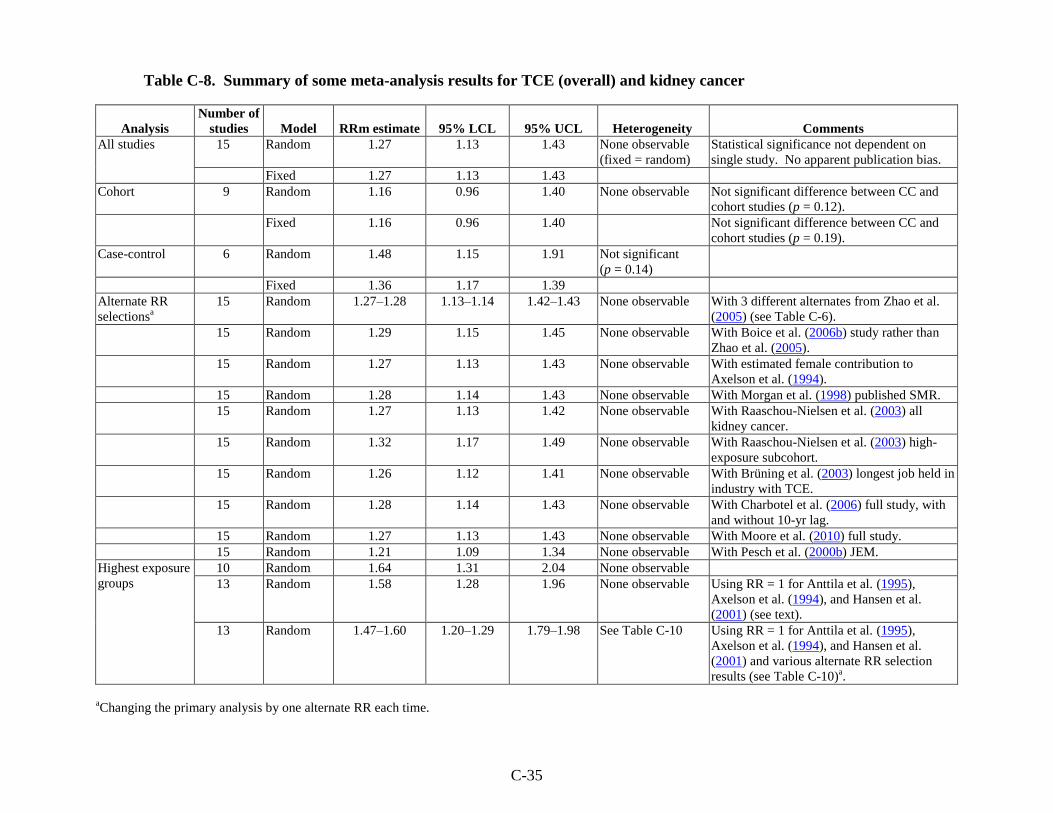
C-35
Table C-8. Summary of some meta-analysis results for TCE (overall) and kidney cancer
Analysis
Number of
studies Model RRm estimate 95% LCL 95% UCL Heterogeneity Comments
All studies 15 Random 1.27 1.13 1.43 None observable
(fixed = random)
Statistical significance not dependent on
single study. No apparent publication bias.
Fixed 1.27 1.13 1.43
Cohort 9 Random 1.16 0.96 1.40 None observable Not significant difference between CC and
cohort studies (p = 0.12).
Fixed 1.16 0.96 1.40 Not significant difference between CC and
cohort studies (p = 0.19).
Case-control 6 Random 1.48 1.15 1.91 Not significant
(p = 0.14)
Fixed 1.36 1.17 1.39
Alternate RR
selectionsa
15 Random 1.27–1.28 1.13–1.14 1.42–1.43 None observable With 3 different alternates from Zhao et al.
(2005) (see Table C-6).
15 Random 1.29 1.15 1.45 None observable With Boice et al. (2006b) study rather than
Zhao et al. (2005).
15 Random 1.27 1.13 1.43 None observable With estimated female contribution to
Axelson et al. (1994).
15 Random 1.28 1.14 1.43 None observable With Morgan et al. (1998) published SMR.
15 Random 1.27 1.13 1.42 None observable With Raaschou-Nielsen et al. (2003) all
kidney cancer.
15 Random 1.32 1.17 1.49 None observable With Raaschou-Nielsen et al. (2003) high-
exposure subcohort.
15 Random 1.26 1.12 1.41 None observable With Brüning et al. (2003) longest job held in
industry with TCE.
15 Random 1.28 1.14 1.43 None observable With Charbotel et al. (2006) full study, with
and without 10-yr lag.
15 Random 1.27 1.13 1.43 None observable With Moore et al. (2010) full study.
15 Random 1.21 1.09 1.34 None observable With Pesch et al. (2000b) JEM.
Highest exposure
groups
10 Random 1.64 1.31 2.04 None observable
13 Random 1.58 1.28 1.96 None observable Using RR = 1 for Anttila et al. (1995),
Axelson et al. (1994), and Hansen et al.
(2001) (see text).
13 Random 1.47–1.60 1.20–1.29 1.79–1.98 See Table C-10 Using RR = 1 for Anttila et al. (1995),
Axelson et al. (1994), and Hansen et al.
(2001) and various alternate RR selection
results (see Table C-10)a.
aChanging the primary analysis by one alternate RR each time.
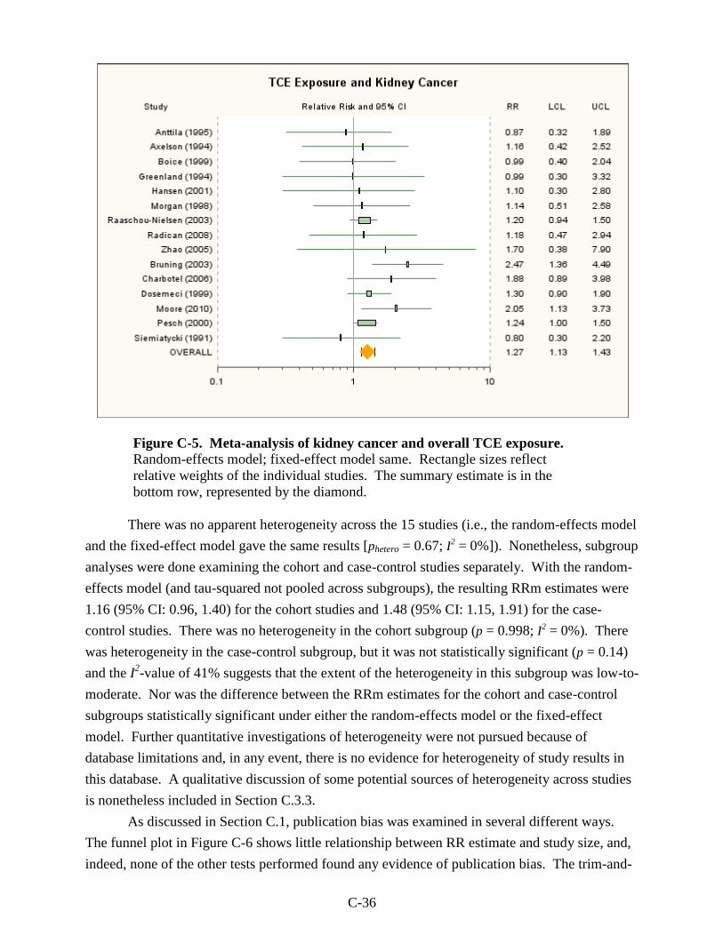
C-36
Figure C-5. Meta-analysis of kidney cancer and overall TCE exposure.
Random-effects model; fixed-effect model same. Rectangle sizes reflect
relative weights of the individual studies. The summary estimate is in the
bottom row, represented by the diamond.
There was no apparent heterogeneity across the 15 studies (i.e., the random-effects model
and the fixed-effect model gave the same results [phetero = 0.67; I2 = 0%]). Nonetheless, subgroup
analyses were done examining the cohort and case-control studies separately. With the random-
effects model (and tau-squared not pooled across subgroups), the resulting RRm estimates were
1.16 (95% CI: 0.96, 1.40) for the cohort studies and 1.48 (95% CI: 1.15, 1.91) for the case-
control studies. There was no heterogeneity in the cohort subgroup (p = 0.998; I2 = 0%). There
was heterogeneity in the case-control subgroup, but it was not statistically significant (p = 0.14)
and the I2-value of 41% suggests that the extent of the heterogeneity in this subgroup was low-to-
moderate. Nor was the difference between the RRm estimates for the cohort and case-control
subgroups statistically significant under either the random-effects model or the fixed-effect
model. Further quantitative investigations of heterogeneity were not pursued because of
database limitations and, in any event, there is no evidence for heterogeneity of study results in
this database. A qualitative discussion of some potential sources of heterogeneity across studies
is nonetheless included in Section C.3.3.
As discussed in Section C.1, publication bias was examined in several different ways.
The funnel plot in Figure C-6 shows little relationship between RR estimate and study size, and,
indeed, none of the other tests performed found any evidence of publication bias. The trim-and-
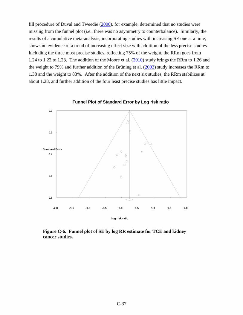
C-37
fill procedure of Duval and Tweedie (2000), for example, determined that no studies were
missing from the funnel plot (i.e., there was no asymmetry to counterbalance). Similarly, the
results of a cumulative meta-analysis, incorporating studies with increasing SE one at a time,
shows no evidence of a trend of increasing effect size with addition of the less precise studies.
Including the three most precise studies, reflecting 75% of the weight, the RRm goes from
1.24 to 1.22 to 1.23. The addition of the Moore et al. (2010) study brings the RRm to 1.26 and
the weight to 79% and further addition of the Brüning et al. (2003) study increases the RRm to
1.38 and the weight to 83%. After the addition of the next six studies, the RRm stabilizes at
about 1.28, and further addition of the four least precise studies has little impact.
Figure C-6. Funnel plot of SE by log RR estimate for TCE and kidney
cancer studies.
-2.0 -1.5 -1.0 -0.5 0.0 0.5 1.0 1.5 2.0
0.0
0.2
0.4
0.6
0.8
Standard Error
Log risk ratio
Funnel Plot of Standard Error by Log risk ratio
C-38
C.3.2. Kidney Cancer Effect in the Highest Exposure Groups
C.3.2.1. Selection of RR Estimates
The selected RR estimates for kidney cancer in the highest TCE exposure categories, for
studies that provided such estimates, are presented in Table C-9. Five of the nine cohort studies
and five of the six case-control studies reported kidney cancer risk estimates categorized by
exposure level. As in Section C.3.1.1 for the overall risk estimates, estimates for RCC were
preferentially selected when presented, and, wherever possible, RR estimates for males and
females combined were used.
Three of the nine cohort studies (Hansen et al., 2001; Anttila et al., 1995; Axelson et al.,
1994) did not report kidney cancer risk estimates categorized by exposure level even though
these same studies reported such estimates for selected other cancer sites. To address this
reporting bias, attempts were made to obtain the results from the primary investigators, and,
failing that, an alternate analysis was performed in which null estimates (RR = 1.0) were
included for all three studies. This alternate analysis was then used as the main analysis, e.g., the
basis of comparison for the sensitivity analyses. For the SE (of the log RR) estimates for these
null estimates, SE estimates from other sites for which highest-exposure-group results were
available were used. For Anttila et al.(1995), the SE estimate for liver cancer in the highest
exposure group was used, because liver cancer and kidney cancer had similar numbers of cases
in the overall study (5 and 6, respectively). For Axelson et al. (1994), the SE estimate for NHL
in the highest exposure group was used, because NHL and kidney cancer had similar numbers of
cases in the overall study (5 and 6, respectively). For Hansen et al. (2001), the SE estimate for
NHL in the highest exposure group was used, because NHL was the only cancer site of interest
in this assessment for which highest-exposure-group results were available.
For Boice et al. (1999), only results for workers with ―any potential exposure‖ (rather
than ―potential routine exposure‖) were presented by exposure category, and the referent group is
workers not exposed to any solvent.
For Morgan et al. (1998), the primary analysis used results for the cumulative exposure
metric, and a sensitivity analysis was done with the results for the peak exposure metric.
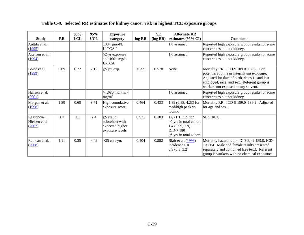
C-39
Table C-9. Selected RR estimates for kidney cancer risk in highest TCE exposure groups
Study RR
95%
LCL
95%
UCL
Exposure
category log RR
SE
(log RR)
Alternate RR
estimates (95% CI) Comments
Anttila et al.
(1995)
100+ µmol/L
U-TCA a
1.0 assumed Reported high exposure group results for some
cancer sites but not kidney.
Axelson et al.
(1994)
≥2-yr exposure
and 100+ mg/L
U-TCA
1.0 assumed Reported high exposure group results for some
cancer sites but not kidney.
Boice et al.
(1999)
0.69 0.22 2.12 ≥5 yrs exp –0.371 0.578 None Mortality RR. ICD-9 189.0–189.2. For
potential routine or intermittent exposure.
Adjusted for date of birth, dates 1st and last
employed, race, and sex. Referent group is
workers not exposed to any solvent.
Hansen et al.
(2001)
≥1,080 months ×
mg/m3
1.0 assumed Reported high exposure group results for some
cancer sites but not kidney.
Morgan et al.
(1998)
1.59 0.68 3.71 High cumulative
exposure score
0.464 0.433 1.89 (0.85, 4.23) for
med/high peak vs.
low/no
Mortality RR. ICD-9 189.0–189.2. Adjusted
for age and sex.
Raaschou-
Nielsen et al.
(2003)
1.7 1.1 2.4 ≥5 yrs in
subcohort with
expected higher
exposure levels
0.531 0.183 1.6 (1.1, 2.2) for
≥5 yrs in total cohort
1.4 (0.99, 1.9)
ICD-7 180
≥5 yrs in total cohort
SIR. RCC.
Radican et al.
(2008)
1.11 0.35 3.49 >25 unit-yrs 0.104 0.582 Blair et al. (1998)
incidence RR
0.9 (0.3, 3.2)
Mortality hazard ratio. ICD-8, -9 189.0, ICD-
10 C64. Male and female results presented
separately and combined (see text). Referent
group is workers with no chemical exposures.
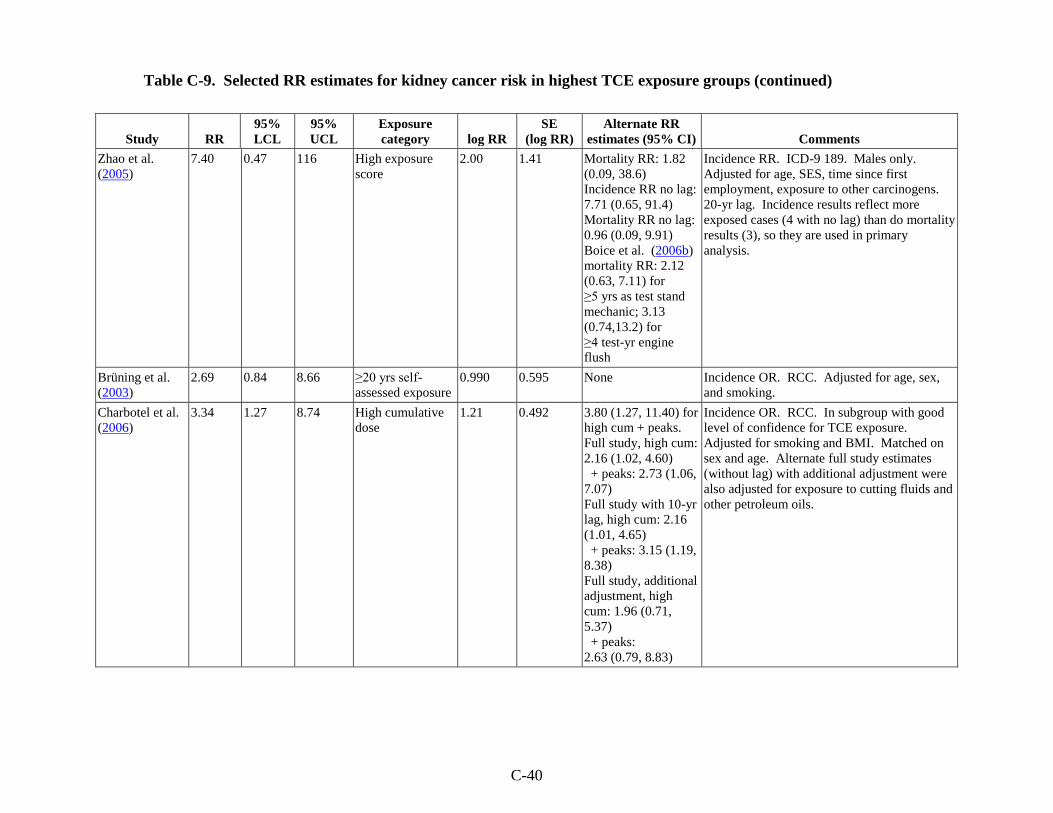
C-40
Table C-9. Selected RR estimates for kidney cancer risk in highest TCE exposure groups (continued)
Study RR
95%
LCL
95%
UCL
Exposure
category log RR
SE
(log RR)
Alternate RR
estimates (95% CI) Comments
Zhao et al.
(2005)
7.40 0.47 116 High exposure
score
2.00 1.41 Mortality RR: 1.82
(0.09, 38.6)
Incidence RR no lag:
7.71 (0.65, 91.4)
Mortality RR no lag:
0.96 (0.09, 9.91)
Boice et al. (2006b)
mortality RR: 2.12
(0.63, 7.11) for
≥5 yrs as test stand
mechanic; 3.13
(0.74,13.2) for
≥4 test-yr engine
flush
Incidence RR. ICD-9 189. Males only.
Adjusted for age, SES, time since first
employment, exposure to other carcinogens.
20-yr lag. Incidence results reflect more
exposed cases (4 with no lag) than do mortality
results (3), so they are used in primary
analysis.
Brüning et al.
(2003)
2.69 0.84 8.66 ≥20 yrs self-
assessed exposure
0.990 0.595 None Incidence OR. RCC. Adjusted for age, sex,
and smoking.
Charbotel et al.
(2006)
3.34 1.27 8.74 High cumulative
dose
1.21 0.492 3.80 (1.27, 11.40) for
high cum + peaks.
Full study, high cum:
2.16 (1.02, 4.60)
+ peaks: 2.73 (1.06,
7.07)
Full study with 10-yr
lag, high cum: 2.16
(1.01, 4.65)
+ peaks: 3.15 (1.19,
8.38)
Full study, additional
adjustment, high
cum: 1.96 (0.71,
5.37)
+ peaks:
2.63 (0.79, 8.83)
Incidence OR. RCC. In subgroup with good
level of confidence for TCE exposure.
Adjusted for smoking and BMI. Matched on
sex and age. Alternate full study estimates
(without lag) with additional adjustment were
also adjusted for exposure to cutting fluids and
other petroleum oils.
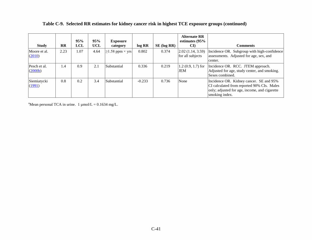
C-41
Table C-9. Selected RR estimates for kidney cancer risk in highest TCE exposure groups (continued)
Study RR
95%
LCL
95%
UCL
Exposure
category log RR SE (log RR)
Alternate RR
estimates (95%
CI) Comments
Moore et al.
(2010)
2.23 1.07 4.64 ≥1.58 ppm × yrs 0.802 0.374 2.02 (1.14, 3.59)
for all subjects
Incidence OR. Subgroup with high-confidence
assessments. Adjusted for age, sex, and
center.
Pesch et al.
(2000b)
1.4 0.9 2.1 Substantial 0.336 0.219 1.2 (0.9, 1.7) for
JEM
Incidence OR. RCC. JTEM approach.
Adjusted for age, study center, and smoking.
Sexes combined.
Siemiatycki
(1991)
0.8 0.2 3.4 Substantial -0.233 0.736 None Incidence OR. Kidney cancer. SE and 95%
CI calculated from reported 90% CIs. Males
only; adjusted for age, income, and cigarette
smoking index.
aMean personal TCA in urine. 1 µmol/L = 0.1634 mg/L.
C-42
For Raaschou-Nielsen et al. (2003), results for RCC in the highest duration subgroup
from the subcohort with expected higher exposure levels (≥1-year duration of employment and
year of 1st employment before 1980) were preferred for the highest-exposure-group analyses.
Results for RCC in the highest duration subgroup from the whole cohort were combined across
sexes, assuming a Poisson distribution, and used in a sensitivity analysis. Also, for the whole
cohort, results for RCC and renal pelvis/ureter cancers in the highest duration group were
combined (across sexes as well), assuming a Poisson distribution, and used in an additional
sensitivity analysis.
For Radican et al. (2008), it should be noted that the referent group is workers with no
chemical exposures, not just no TCE exposure. In addition, results for exposure groups (based
on cumulative exposure scores) were reported separately for males and females and were
combined for this assessment using inverse-variance weighting, as in a fixed-effect meta-
analysis. Radican et al. (2008) present only mortality hazard ratio estimates by exposure group;
however, in an earlier follow-up of this same cohort, Blair et al. (1998) present both incidence
and mortality RR estimates by exposure group. The mortality RR estimate based on the more
recent follow-up by Radican et al. (2008) (six deaths in the highest exposure group) was used in
the primary analysis, while the incidence RR estimate based on similarly combined results from
Blair et al. (1998) (four cases) was used as an alternate estimate in a sensitivity analysis.
Radican et al. (2008) also present results for categories based on frequency and pattern of
exposure; however, subjects weren‘t distributed uniquely across the categories (the numbers of
cases across categories exceeded the total number of cases); thus, it was difficult to interpret
these results and they were not used in a sensitivity analysis.
Zhao et al. (2005) present kidney cancer RR estimates adjusted for exposure to other
carcinogens, because, unlike for NHL, this adjustment made a considerable difference.
Estimates of RR with this additional adjustment were selected over those without. Furthermore,
the kidney results were presented with and without a 20-year lag. A 20-year lag seemed
reasonable for kidney cancer, so the lagged estimates were preferred to the unlagged; unlagged
estimates were used in sensitivity analyses. In addition, the incidence results reflect more cases
(4 with no lag) in the highest exposure group than do the mortality results (3), so the incidence
result (with the 20-year lag) was used for the primary analysis, and the unlagged incidence result
and the mortality results were used in a sensitivity analysis. Sensitivity analyses were also done
using results from Boice et al. (2006b) in place of the Zhao et al. (2005) RR estimate. The
cohorts for these studies overlap, so they are not independent studies. Boice et al. (2006b) report
mortality RR estimates for kidney cancer by years worked as a test stand mechanic, a job with
potential TCE exposure, and by a measure that weighted years with potential exposure from
engine flushing by the number of flushes each year. No results were presented for a third metric,
years worked with potential exposure to any TCE, because the Cox proportional hazards model
C-43
did not converge. The Boice et al. (2006b) estimates are adjusted for years of birth and hire and
for hydrazine exposure.
For Charbotel et al. (2006), results from the analysis that considered ―only job periods
with a good level of confidence for TCE exposure assessment‖ [Table 7 of Charbotel et al.
(2006)] were preferred, as these estimates would presumably be less influenced by exposure
misclassification. Additionally, the high cumulative dose results were preferred, but the results
for high cumulative dose + peaks were included in a sensitivity analysis. Exposure group results
with a 10-year lag are provided in an unpublished report (Charbotel et al., 2005); however,
lagged results are presented only for the full study and, thus, were used in sensitivity analyses.
Estimates from the full study analysis (without the lag) that were further adjusted for exposure to
cutting fluids and other petroleum oils were also used in sensitivity analyses.
Similarly, for Moore et al. (2010), results from the analysis that considered high-
confidence assessments only were preferred. Here the definition of TCE exposure was restricted
to jobs classified as having probable or certain exposure (i.e., at least 40% of workers with that
job were expected to be exposed), so these estimates should be less influenced by exposure
misclassification. Estimates from the analysis of all subjects were used in a sensitivity analysis.
The highest exposure group was reported as ≥1.58 ppm × years; however, this value is not based
on continuous exposure estimates but rather calculated from midpoints of estimated ranges
corresponding to categorical groups, i.e., cumulative exposure = categorical intensity weight
(ppm) × categorical frequency weight × duration (years).
For Pesch et al. (2000b), TCE results were presented for two different exposure
assessments. As discussed above, estimates using the JTEM approach were preferred because
they seemed to represent a more comprehensive exposure assessment; estimates based on the
JEM approach were used in a sensitivity analysis.
C.3.2.2. Results of Meta-Analyses
Results from the meta-analyses that were conducted for kidney cancer in the highest
exposure groups are summarized at the bottom of Table C-8 and reported in more detail in
Table C-10. The RRm estimate from the random-effects meta-analysis of the 10 studies with
results presented for exposure groups was 1.64 (95% CI: 1.31, 2.04). The RRm estimate from
the primary random-effects meta-analysis with null RR estimates (i.e., 1.0) included for Anttila
et al. (1995), Axelson et al. (1994), and Hansen et al. (2001) to address reporting bias (see above)
was 1.58 (95% CI: 1.28, 1.96) (see Figure C-7). The inclusion of these three additional studies
contributed just over 7% of the total weight. As with the overall kidney cancer meta-analyses,
the meta-analyses of the highest exposure groups were dominated by two studies (Raaschou-
Nielsen et al., 2003; Pesch et al., 2000b), which provided about 60% of the weight. No single
study was overly influential; removal of individual studies resulted in RRm estimates that were
C-44
all statistically significant (all with p < 0.005) and that ranged from 1.52 [with the removal of
Raaschou-Nielsen et al. (2003)] to 1.64 [with the removal of Pesch et al. (2000b)].
Similarly, the RRm estimate was not highly sensitive to alternate RR estimate selections.
Use of the 18 alternate selections, individually, resulted in RRm estimates that were all
statistically significant (all with p < 0.0005) and that ranged from 1.47 to 1.60, with all but two
of the alternate selections yielding RRm estimates in the narrow range of 1.54–1.60 (see
Table C-10). The lowest RRm estimates, 1.47 in both cases, were obtained when the alternate
selections involved the two large studies. One of the alternate selections was for Raaschou-
Nielsen et al. (2003), with a highest-exposure-group estimate for all kidney cancer in the total
cohort, rather than RCC in the subcohort expected to have higher exposure levels. The latter
value is strongly preferred because, as discussed above, the subcohort is likely to have less
exposure misclassification. Furthermore, RCC is very different from other types of kidney
cancer, and TCE, if an etiological factor, may not be etiologically associated with all kidney
cancers, so using the broad category may dilute a true association with RCC, if one exists. The
other alternate selection with a considerable impact on the RRm estimate was for Pesch et al.
(2000b), with the highest exposure group result based on the JEM exposure assessment
approach, rather than the JTEM approach. As discussed above, the JTEM approach is preferred
because it seemed to be a more comprehensive and discriminating approach, taking actual job
tasks into account, rather than just larger job categories. Thus, although results with these
alternate selections are presented for comprehensiveness and transparency, the primary analysis
is believed to reflect better the potential association between kidney cancer (in particular, RCC)
and TCE exposure.
Other than a negligible amount of heterogeneity observed in the sensitivity analysis with
the Pesch et al. (2000b) JEM alternate discussed above (I2 = 0.64%), there was no observable
heterogeneity across the studies for any of the meta-analyses conducted with the highest
exposure groups, including those in which RR values for Anttila et al.(1995), Axelson et al.
(1994), and Hansen et al. (2001) were assumed. No subgroup analyses (e.g., cohort vs. case-
control studies) were done with the highest exposure group results.
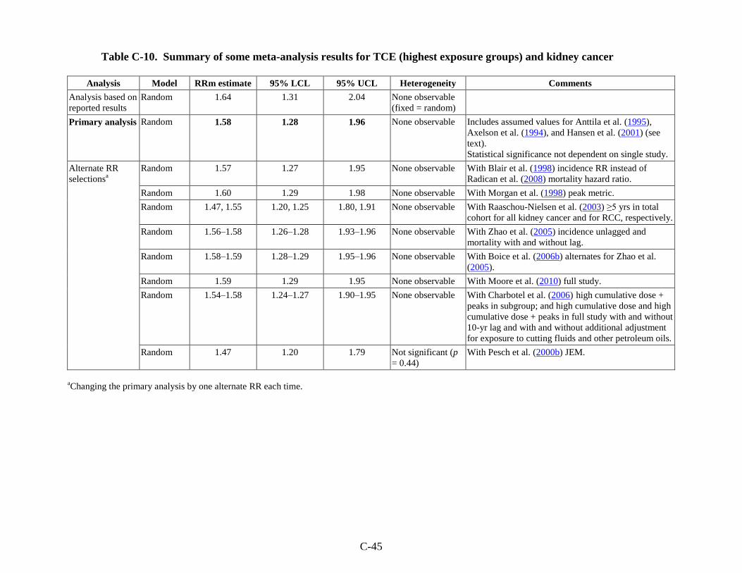
C-45
Table C-10. Summary of some meta-analysis results for TCE (highest exposure groups) and kidney cancer
Analysis Model RRm estimate 95% LCL 95% UCL Heterogeneity Comments
Analysis based on
reported results
Random 1.64 1.31 2.04 None observable
(fixed = random)
Primary analysis Random 1.58 1.28 1.96 None observable
Includes assumed values for Anttila et al. (1995),
Axelson et al. (1994), and Hansen et al. (2001) (see
text).
Statistical significance not dependent on single study.
Alternate RR
selectionsa
Random 1.57 1.27 1.95 None observable With Blair et al. (1998) incidence RR instead of
Radican et al. (2008) mortality hazard ratio.
Random 1.60 1.29 1.98 None observable With Morgan et al. (1998) peak metric.
Random 1.47, 1.55 1.20, 1.25 1.80, 1.91 None observable With Raaschou-Nielsen et al. (2003) ≥5 yrs in total
cohort for all kidney cancer and for RCC, respectively.
Random 1.56–1.58 1.26–1.28 1.93–1.96 None observable With Zhao et al. (2005) incidence unlagged and
mortality with and without lag.
Random 1.58–1.59 1.28–1.29 1.95–1.96 None observable With Boice et al. (2006b) alternates for Zhao et al.
(2005).
Random 1.59 1.29 1.95 None observable With Moore et al. (2010) full study.
Random 1.54–1.58 1.24–1.27 1.90–1.95 None observable With Charbotel et al. (2006) high cumulative dose +
peaks in subgroup; and high cumulative dose and high
cumulative dose + peaks in full study with and without
10-yr lag and with and without additional adjustment
for exposure to cutting fluids and other petroleum oils.
Random 1.47 1.20 1.79 Not significant (p
= 0.44)
With Pesch et al. (2000b) JEM.
aChanging the primary analysis by one alternate RR each time.
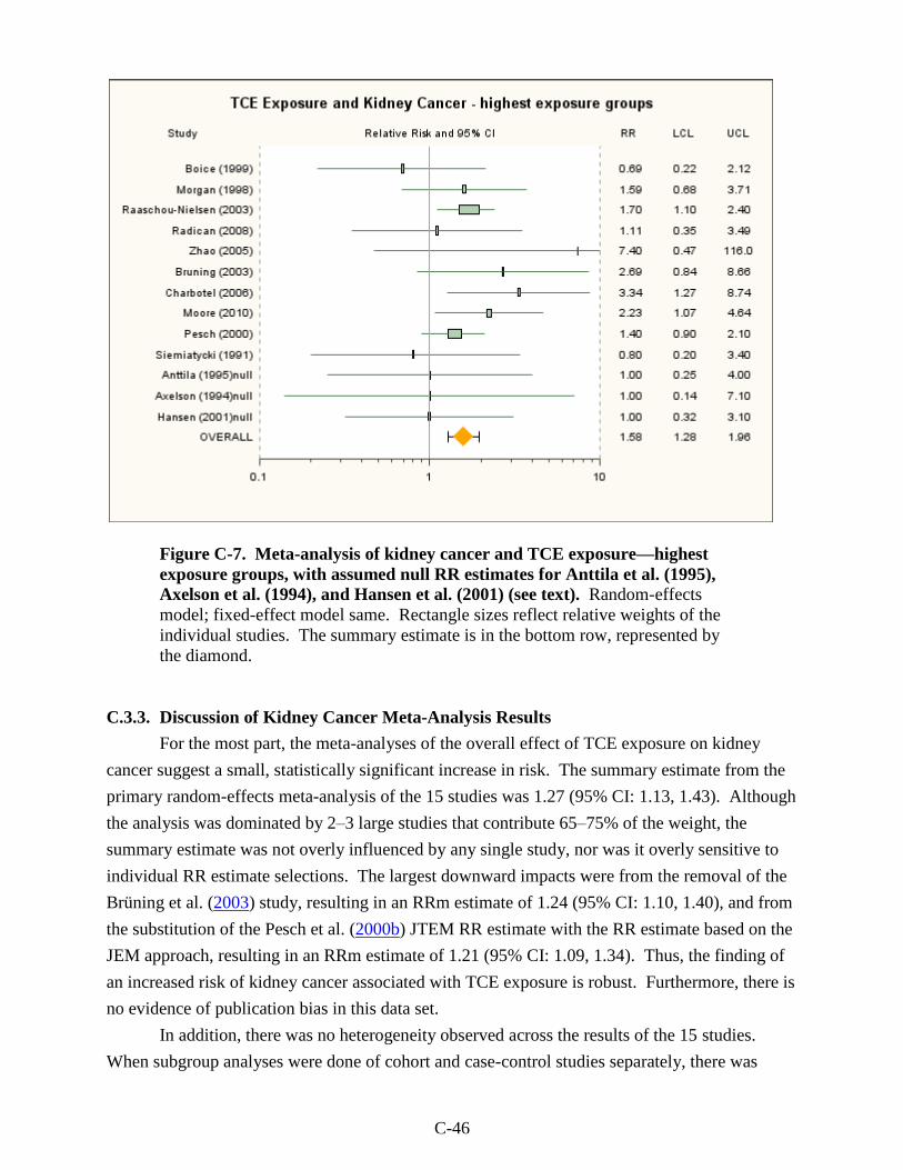
C-46
Figure C-7. Meta-analysis of kidney cancer and TCE exposure—highest
exposure groups, with assumed null RR estimates for Anttila et al. (1995),
Axelson et al. (1994), and Hansen et al. (2001) (see text). Random-effects
model; fixed-effect model same. Rectangle sizes reflect relative weights of the
individual studies. The summary estimate is in the bottom row, represented by
the diamond.
C.3.3. Discussion of Kidney Cancer Meta-Analysis Results
For the most part, the meta-analyses of the overall effect of TCE exposure on kidney
cancer suggest a small, statistically significant increase in risk. The summary estimate from the
primary random-effects meta-analysis of the 15 studies was 1.27 (95% CI: 1.13, 1.43). Although
the analysis was dominated by 2–3 large studies that contribute 65–75% of the weight, the
summary estimate was not overly influenced by any single study, nor was it overly sensitive to
individual RR estimate selections. The largest downward impacts were from the removal of the
Brüning et al. (2003) study, resulting in an RRm estimate of 1.24 (95% CI: 1.10, 1.40), and from
the substitution of the Pesch et al. (2000b) JTEM RR estimate with the RR estimate based on the
JEM approach, resulting in an RRm estimate of 1.21 (95% CI: 1.09, 1.34). Thus, the finding of
an increased risk of kidney cancer associated with TCE exposure is robust. Furthermore, there is
no evidence of publication bias in this data set.
In addition, there was no heterogeneity observed across the results of the 15 studies.
When subgroup analyses were done of cohort and case-control studies separately, there was
C-47
some observable heterogeneity among the case-control studies, but it was not statistically
significant (p = 0.14) and the I2-value of 41% suggested the extent of the heterogeneity was low-
to-moderate. The increased risk of kidney cancer was strengthened in the case-control study
analysis and weakened in the cohort study analysis, but the difference between the two RRm
estimates was not statistically significant. One difference between the case-control and cohort
studies is that the case-control studies were of RCC and almost all of the cohort studies were of
all kidney cancers, including renal pelvis. As discussed above, RCC is very different from other
types of kidney cancer, and TCE, if an etiological factor, may not be etiologically associated
with all kidney cancers, so using the broad category may dilute a true association with RCC, if
one exists.
With respect to the nonsignificant heterogeneity in the six case-control studies, these
studies differ in TCE exposure potential to the underlying population from which case and
control subjects were identified, and this may be a source of some heterogeneity. Prevalence of
exposure to TCE among cases in these studies was 27% in Charbotel et al. (2006) (for high-
level-of-confidence jobs), 18% in Brüning et al. (2003) (for self-assessed exposure), 18% in
Pesch et al. (2000b), 13% in Dosemeci et al. (1999), 3.6% in Moore et al. (2010) (for high-
confidence jobs), and 1% in Siemiatycki (1991). Both Brüning et al. (2003) and Charbotel et al.
(2006) are studies designed specifically to assess RCC and TCE exposure. These studies were
carried out in geographical areas with both a high prevalence and a high degree of TCE
exposure. Some information is provided in these and accompanying papers to describe the
nature of exposure, making it possible to estimate the order of magnitude of exposure, even
though there were no direct measurements (Fevotte et al., 2006; Brüning et al., 2003; Cherrie et
al., 2001). The Charbotel et al. (2006) study was carried out in the Arve Valley region in France,
where TCE exposure was through metal-degreasing activity in small shops involved in the
manufacturing of screws and precision metal parts (Fevotte et al., 2006). Industrial hygiene data
from shops in this area indicated high intensity TCE exposures of ≥100 ppm, particularly from
exposures from hot degreasing processes. Considering exposure only from the jobs with a high
level of confidence about exposure, 18% of exposed cases were identified with high cumulative
exposure to TCE. The source population in the Brüning et al. (2003) study includes the
Arnsberg region in Germany, which also has a high prevalence of TCE exposure. A large
number of small companies used TCE in metal degreasing in small workrooms. Subjects in this
study also described neurological symptoms previously associated with higher TCE intensities.
While subjects in the Brüning et al. (2003) study had potential high TCE exposure intensity,
average TCE exposure in this study is considered lower than that in the Charbotel et al. (2006)
study because the base population was enlarged beyond the Arnsberg region to areas which did
not have the same focus of industry.
Siemiatycki (1991), Dosemeci et al. (1999), and Pesch et al. (2000b) are population-
based studies. Sources of exposure to TCE and other chlorinated solvents are much less well
C-48
defined in these studies, and most subjects identified with TCE exposure probably had minimal
contact; estimated average concentrations to exposed subjects were of about 10 ppm or less
(NRC, 2006). Pesch et al. (2000b) includes the Arnsberg area and four other regions. Neither
Dosemeci et al. (1999) nor Siemiatycki (1991) describe the nature of the TCE exposure. TCE
exposure potential in these two studies is likely lower than in the other studies and closer to
background. Furthermore, the use of generic job-exposure-matrices for exposure assessment in
these studies may result in a greater potential for exposure misclassification bias.
Moore et al. (2010) is a hospital-based study which identified subjects from four Eastern
and Central European countries with high kidney cancer rates (Czech Republic, Poland, Russia,
and Romania). In their exposure assessment, Moore et al. (2010) accounted for the likelihood of
TCE exposure, defined as possible, probable, or definite exposure. This likely increased
exposure potential in their subgroup of high-confidence TCE assessments, which was restricted
to subjects with probable or definite exposure. Although their semi-quantitative exposure
assessment most probably improved exposure rankings, TCE exposure potential is likely lower
in their study than in Brüning et al. (2003) and Charbotel et al. (2006), given the many jobs and
industries included.
Ten of the 15 studies categorized results by exposure level. Three other studies reported
results for other cancer sites by exposure level, but not kidney cancer; thus, to address this
reporting bias, null values (i.e., RR estimates of 1.0) were used for these studies. Different
exposure metrics were used in the various studies, and the purpose of combining results across
the different highest exposure groups was not to estimate an RRm associated with some level of
exposure, but rather to see the impacts of combining RR estimates that should be less affected by
exposure misclassification. In other words, the highest exposure category is more likely to
represent a greater differential TCE exposure compared to people in the referent group than the
exposure differential for the overall (typically any vs. none) exposure comparison. Thus, if TCE
exposure increases the risk of kidney cancer, the effects should be more apparent in the highest
exposure groups. Indeed, the RRm estimate from the primary meta-analysis of the highest
exposure group results was 1.58 (95% CI: 1.28, 1.96), which is greater than the RRm estimate of
1.27 (95% CI: 1.13, 1.43) from the overall exposure analysis. This result for the highest
exposure groups was not overly influenced by any single study, nor was it overly sensitive to
individual RR estimate selections. Heterogeneity was not observed in any of the analyses, with
the exception of some negligible heterogeneity (I2 = 0.64%) in one sensitivity analysis. The
robustness of this finding lends substantial support to a conclusion that TCE exposure increases
the risk of kidney cancer.
C-49
C.4. META-ANALYSIS FOR LIVER CANCER
C.4.1. Overall Effect of TCE Exposure
C.4.1.1. Selection of RR Estimates
The selected RR estimates for liver cancer associated with TCE exposure from the
epidemiological studies are presented in Table C-11. There were no case-control studies for
liver cancer and TCE exposure that were selected for inclusion in the meta-analysis (see
Appendix B, Section B.2.9), so all of the relevant studies are cohort studies. All of the studies
reported results for liver cancers plus cancers of the gall bladder and extrahepatic biliary
passages (i.e., ICD-7 155.0 + 155.2; ICD-8 and -9 155 + 156). Three of the studies also report
results for liver cancer alone (ICD-7 155.0; ICD-8 and -9 155). For the primary analysis, results
for cancers of the liver, gall bladder, and biliary passages combined were selected, for the sake of
consistency, since these were reported in all of the studies. An alternate analysis was also done
using results for liver cancer alone for the three studies that reported them and the combined liver
cancer results for the remainder of the studies.
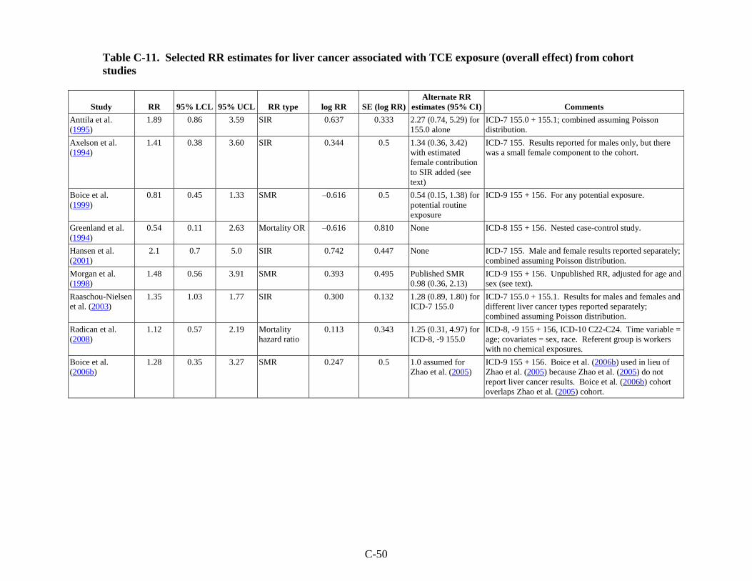
C-50
Table C-11. Selected RR estimates for liver cancer associated with TCE exposure (overall effect) from cohort
studies
Study RR 95% LCL 95% UCL RR type log RR SE (log RR)
Alternate RR
estimates (95% CI) Comments
Anttila et al.
(1995)
1.89 0.86 3.59 SIR 0.637 0.333 2.27 (0.74, 5.29) for
155.0 alone
ICD-7 155.0 + 155.1; combined assuming Poisson
distribution.
Axelson et al.
(1994)
1.41 0.38 3.60 SIR 0.344 0.5 1.34 (0.36, 3.42)
with estimated
female contribution
to SIR added (see
text)
ICD-7 155. Results reported for males only, but there
was a small female component to the cohort.
Boice et al.
(1999)
0.81 0.45 1.33 SMR –0.616 0.5 0.54 (0.15, 1.38) for
potential routine
exposure
ICD-9 155 + 156. For any potential exposure.
Greenland et al.
(1994)
0.54 0.11 2.63 Mortality OR –0.616 0.810 None ICD-8 155 + 156. Nested case-control study.
Hansen et al.
(2001)
2.1 0.7 5.0 SIR 0.742 0.447 None ICD-7 155. Male and female results reported separately;
combined assuming Poisson distribution.
Morgan et al.
(1998)
1.48 0.56 3.91 SMR 0.393 0.495 Published SMR
0.98 (0.36, 2.13)
ICD-9 155 + 156. Unpublished RR, adjusted for age and
sex (see text).
Raaschou-Nielsen
et al. (2003)
1.35 1.03 1.77 SIR 0.300 0.132 1.28 (0.89, 1.80) for
ICD-7 155.0
ICD-7 155.0 + 155.1. Results for males and females and
different liver cancer types reported separately;
combined assuming Poisson distribution.
Radican et al.
(2008)
1.12 0.57 2.19 Mortality
hazard ratio
0.113 0.343 1.25 (0.31, 4.97) for
ICD-8, -9 155.0
ICD-8, -9 155 + 156, ICD-10 C22-C24. Time variable =
age; covariates = sex, race. Referent group is workers
with no chemical exposures.
Boice et al.
(2006b)
1.28 0.35 3.27 SMR 0.247 0.5 1.0 assumed for
Zhao et al. (2005)
ICD-9 155 + 156. Boice et al. (2006b) used in lieu of
Zhao et al. (2005) because Zhao et al. (2005) do not
report liver cancer results. Boice et al. (2006b) cohort
overlaps Zhao et al. (2005) cohort.
C-51
As for NHL and kidney cancer, many of the studies provided RR estimates only for
males and females combined, and we are not aware of any basis for a sex difference in the
effects of TCE on liver cancer risk; thus, wherever possible, RR estimates for males and females
combined were used. The only study of much size (in terms of number of liver cancer cases)
that provided results separately by sex was Raaschou-Nielsen et al. (2003). The results of this
study suggest that liver cancer risk in females might be slightly higher than the risk in males, but
the number of female cases is small (primary liver cancer SIR: males 1.1 [95% CI: 0.74, 1.64;
27 cases], females 2.8 [95% CI: 1.13, 5.80; 7 cases]; gallbladder and biliary passage cancers SIR:
males 1.1 [95% CI: 0.61, 1.87; 14 cases]; females 2.8 [1.28, 5.34; 9 cases]). Radican et al.
(2008) report hazard ratios for liver/biliary passage cancers combined of 1.36 (95% CI: 0.59,
3.11; 28 deaths) for males and 0.74 (95% CI: 0.18, 2.97; 3 deaths) for females, but these results
are based on fewer cases, especially in females.
Most of the selections in Table C-11 should be self-evident, but some are discussed in
more detail here, in the order the studies are presented in the table. For Axelson et al. (1994), in
which a small subcohort of females was studied but only results for the larger male subcohort
were reported, the reported male-only results were used in the primary analysis; however, as for
NHL and kidney cancer, an attempt was made to estimate the female contribution to an overall
RR estimate for both sexes and its impact on the meta-analysis. Axelson et al. (1994) reported
that there were no cases of liver cancer observed in females, but the expected number was not
presented. To estimate the expected number, the expected number for males was multiplied by
the ratio of female-to-male person-years in the study and by the ratio of female-to-male age-
adjusted incidence rates for liver cancer.8 The male results and the estimated female contribution
were then combined into an RR estimate for both sexes assuming a Poisson distribution, and this
alternate RR estimate for the Axelson et al. (1994) study was used in a sensitivity analysis.
For Boice et al. (1999), results for ―any potential exposure‖ were selected for the primary
analysis, because this exposure category was considered to best represent overall TCE exposure,
and results for ―potential routine exposure,‖ which was characterized as reflecting workers
assumed to have received more cumulative exposure, were used in a sensitivity analysis. To
estimate the SE (log RR) for the primary RR selection, it was assumed that the number of
exposed cases (deaths) was 15. The actual number was not presented, but 15 was the number
that allowed us to reproduce the reported CIs. The number suggested by exposure level in Boice
8Person-years for men and women <79 years were obtained from Axelson et al. (1994): 23,516.5 and 3,691.5,
respectively. Lifetime age-adjusted incidence rates for liver cancer for men and women were obtained from the
National Cancer Institute‘s 2000-2004 SEER-17 (Surveillance Epidemiology and End Results from 17 geographical
areas) database (http://seer.cancer.gov/statfacts/html/livibd.html): 9.5/100,000 and 3.4/100,000, respectively. The
calculation for estimating the expected number of cases in females in the cohort assumes that the males and females
have similar TCE exposures and that the relative distributions of age-related incidence risk for the males and
females in the Swedish cohort are adequately represented by the ratios of person-years and lifetime U.S. incidence
rates used in the calculation.
C-52
et al. (1999) Table 9 is 13; however, it may be that exposure level data were not available for all
of the cases.
In their published paper, Morgan et al. (1998) present only SMRs for overall TCE
exposure, although the results from internal analyses are presented for exposure subgroups. RR
estimates for overall TCE exposure from the internal analyses of the Morgan et al. (1998) cohort
data were available from an unpublished report (EHS, 1997); from these, the RR estimate from
the Cox model that included age and sex was selected, because those are the variables deemed to
be important in the published paper. The internal analysis RR estimate was preferred for the
primary analysis, and the published SMR result was used in a sensitivity analysis.
Raaschou-Nielsen et al. (2003) reported results for primary liver cancer (ICD-7 155.0),
gallbladder and biliary passage cancers (ICD-7 155.1), and unspecified liver cancers (ICD-7 156)
separately. As discussed above, RR estimates for cancers of the liver, gall bladder, and biliary
passages combined were preferred for the primary analysis; thus, the results for primary liver
cancer and gallbladder/biliary passage cancers were combined (across sexes as well), assuming a
Poisson distribution. The results for primary liver cancer only (similarly combined across sexes)
were used in an alternate analysis. The results for unspecified liver cancers (ICD-7 156) were
not included in any analyses because, under the ICD-7 coding, 156 can include secondary liver
cancers. Raaschou-Nielsen et al. (2003), in their Table 3, also present overall results for primary
liver cancer and gallbladder/biliary passage cancers with a lag time of 20 years; however, they
use a definition of lag that is different from a lagged exposure in which exposures prior to
disease onset are discounted and it is not clear what their lag time actually represents9, thus, as
for NHL and kidney cancer, these results were not used in any of the meta-analyses for liver
cancer. In addition, results for the subcohort with expected higher exposure levels were not
provided for liver cancer, so no alternate analysis was done based on the subcohort.
For Radican et al. (2008), the Cox model hazard ratio from the 2000 follow-up was used.
In the Radican et al. (2008) Cox regressions, age was the time variable, and sex and race were
covariates. It should also be noted that the referent group is composed of workers with no
chemical exposures, not just no exposure to TCE.
Zhao et al. (2005) did not present RR estimates for liver cancer; thus, results from Boice
et al. (2006b) were used in the primary analysis. The cohorts for these studies overlap, so they
are not independent studies. Zhao et al. (2005), however, was our preferred study for NHL and
kidney cancer results; thus, in a sensitivity analysis, a null value (RR = 1.0) was assumed for
Zhao et al. (2005) to address the potential reporting bias. The SE estimate for kidney cancer
(incidence with 0 lag) was used as the SE for the liver cancer. (It is not certain that there was a
reporting bias in this case. In the ―Methods‖ section of their paper, Zhao et al. [(2005) list the
9In their Methods section, Raaschou-Nielsen et al. (2003) define their lag period as the period ―from the date of first
employment to the start of follow-up for cancer‖.
C-53
cancer sites examined in the cohort, and liver was not listed; it is not clear if the list of sites was
determined a priori or post hoc.)
Also, on the issue of potential reporting bias, the Siemiatycki (1991) study should be
mentioned. This study was a case-control study for multiple cancer sites, but only the more
common sites, in order to have greater statistical power. Thus, NHL and kidney cancer results
were available, but not liver cancer results. Because no liver results were presented for any of
the chemicals, this is not a case of reporting bias.
C.4.1.2. Results of Meta-Analyses
Results from some of the meta-analyses that were conducted on the epidemiological
studies of TCE and liver cancer are summarized in Table C-12. The RRm from the primary
random-effects meta-analysis of the nine studies was 1.29 (95% CI: 1.07, 1.56) (see Figure C-8).
As shown in Figure C-8, the analysis was dominated by one large study (contributing about 53%
of the weight). That large study was critical in terms of the statistical significance of the RRm
estimate. Without the large Raaschou-Nielsen et al. (2003) study, the RRm estimate decreases
somewhat and is no longer statistically significant (RRm = 1.22; 95% CI: 0.93, 1.61). No other
single study was overly influential; removal of any of the other individual studies resulted in
RRm estimates that were all statistically significant (all with p ≤0.03) and that ranged from 1.24
[with the removal of Anttila et al. (1995)] to 1.39 [with the removal of Boice et al. (1999)].
As discussed in Section C.4.1.1, all of the nine studies presented results for liver and gall
bladder/biliary passage cancers combined, and these results were the basis for the primary
analysis discussed above. An alternate analysis was performed substituting, simultaneously,
results for liver cancer alone for the three studies for which these were available. The RRm
estimate from this analysis was slightly lower than the one based entirely on results from the
combined cancer categories and was just short of statistical significance (1.25; 95% CI: 0.99,
1.57). This result was driven by the fact that the RR estimate from the large Raaschou-Nielsen et
al. (2003) study decreased from 1.35 for liver and gall bladder/biliary passage cancers combined
to 1.28 for liver cancer alone.
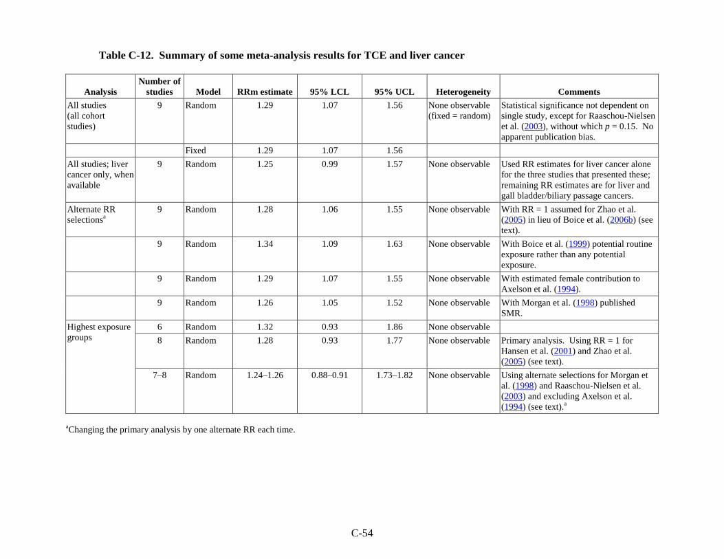
C-54
Table C-12. Summary of some meta-analysis results for TCE and liver cancer
Analysis
Number of
studies Model RRm estimate 95% LCL 95% UCL Heterogeneity Comments
All studies
(all cohort
studies)
9 Random 1.29 1.07 1.56 None observable
(fixed = random)
Statistical significance not dependent on
single study, except for Raaschou-Nielsen
et al. (2003), without which p = 0.15. No
apparent publication bias.
Fixed 1.29 1.07 1.56
All studies; liver
cancer only, when
available
9 Random 1.25 0.99 1.57 None observable Used RR estimates for liver cancer alone
for the three studies that presented these;
remaining RR estimates are for liver and
gall bladder/biliary passage cancers.
Alternate RR
selectionsa
9 Random 1.28 1.06 1.55 None observable With RR = 1 assumed for Zhao et al.
(2005) in lieu of Boice et al. (2006b) (see
text).
9 Random 1.34 1.09 1.63 None observable With Boice et al. (1999) potential routine
exposure rather than any potential
exposure.
9 Random 1.29 1.07 1.55 None observable With estimated female contribution to
Axelson et al. (1994).
9 Random 1.26 1.05 1.52 None observable With Morgan et al. (1998) published
SMR.
Highest exposure
groups
6 Random 1.32 0.93 1.86 None observable
8 Random 1.28 0.93 1.77 None observable Primary analysis. Using RR = 1 for
Hansen et al. (2001) and Zhao et al.
(2005) (see text).
7–8 Random 1.24–1.26 0.88–0.91 1.73–1.82 None observable Using alternate selections for Morgan et
al. (1998) and Raaschou-Nielsen et al.
(2003) and excluding Axelson et al.
(1994) (see text).a
aChanging the primary analysis by one alternate RR each time.
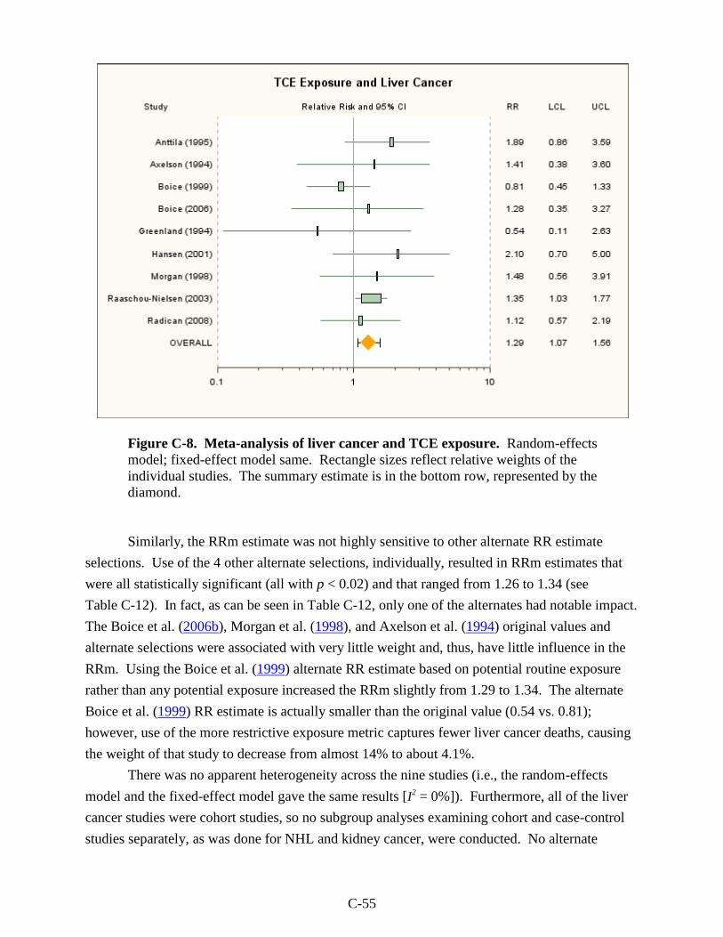
C-55
Figure C-8. Meta-analysis of liver cancer and TCE exposure. Random-effects
model; fixed-effect model same. Rectangle sizes reflect relative weights of the
individual studies. The summary estimate is in the bottom row, represented by the
diamond.
Similarly, the RRm estimate was not highly sensitive to other alternate RR estimate
selections. Use of the 4 other alternate selections, individually, resulted in RRm estimates that
were all statistically significant (all with p < 0.02) and that ranged from 1.26 to 1.34 (see
Table C-12). In fact, as can be seen in Table C-12, only one of the alternates had notable impact.
The Boice et al. (2006b), Morgan et al. (1998), and Axelson et al. (1994) original values and
alternate selections were associated with very little weight and, thus, have little influence in the
RRm. Using the Boice et al. (1999) alternate RR estimate based on potential routine exposure
rather than any potential exposure increased the RRm slightly from 1.29 to 1.34. The alternate
Boice et al. (1999) RR estimate is actually smaller than the original value (0.54 vs. 0.81);
however, use of the more restrictive exposure metric captures fewer liver cancer deaths, causing
the weight of that study to decrease from almost 14% to about 4.1%.
There was no apparent heterogeneity across the nine studies (i.e., the random-effects
model and the fixed-effect model gave the same results [I2 = 0%]). Furthermore, all of the liver
cancer studies were cohort studies, so no subgroup analyses examining cohort and case-control
studies separately, as was done for NHL and kidney cancer, were conducted. No alternate
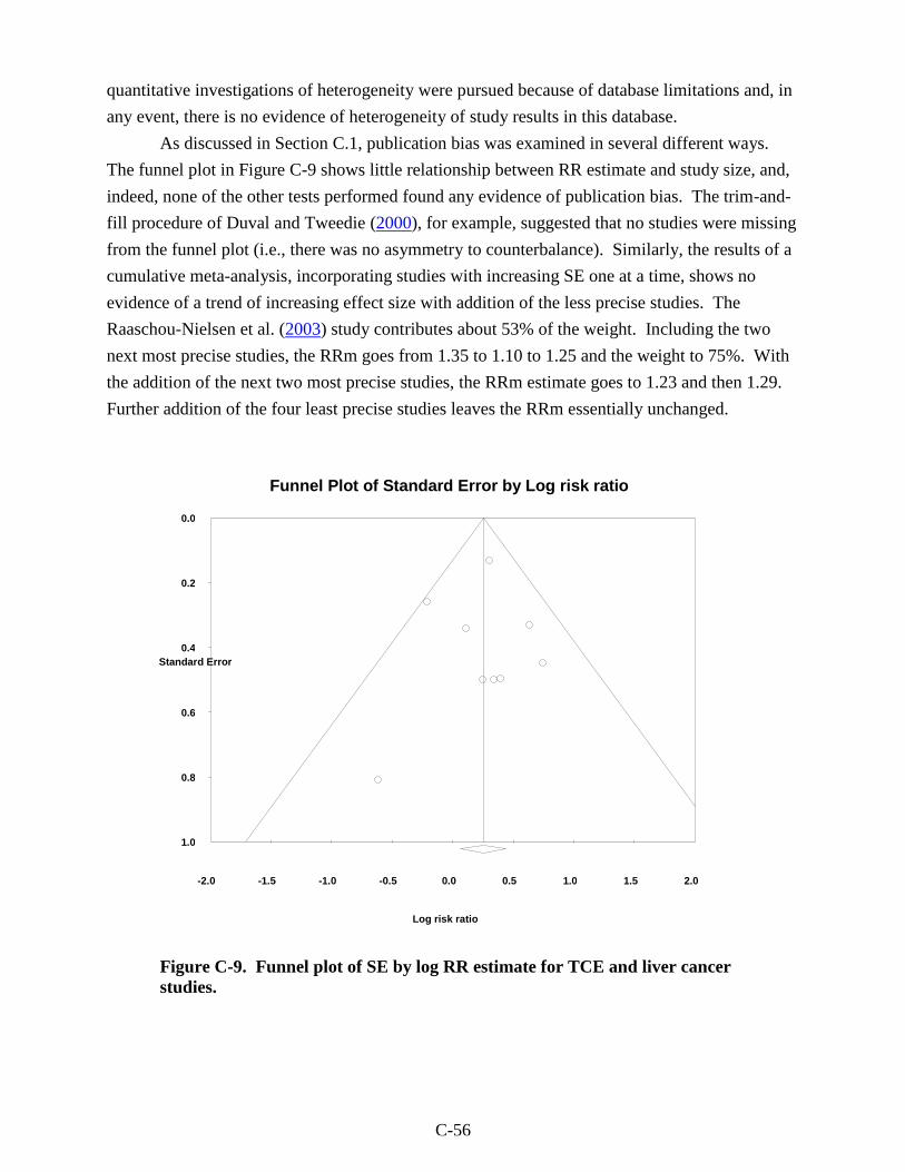
C-56
quantitative investigations of heterogeneity were pursued because of database limitations and, in
any event, there is no evidence of heterogeneity of study results in this database.
As discussed in Section C.1, publication bias was examined in several different ways.
The funnel plot in Figure C-9 shows little relationship between RR estimate and study size, and,
indeed, none of the other tests performed found any evidence of publication bias. The trim-and-
fill procedure of Duval and Tweedie (2000), for example, suggested that no studies were missing
from the funnel plot (i.e., there was no asymmetry to counterbalance). Similarly, the results of a
cumulative meta-analysis, incorporating studies with increasing SE one at a time, shows no
evidence of a trend of increasing effect size with addition of the less precise studies. The
Raaschou-Nielsen et al. (2003) study contributes about 53% of the weight. Including the two
next most precise studies, the RRm goes from 1.35 to 1.10 to 1.25 and the weight to 75%. With
the addition of the next two most precise studies, the RRm estimate goes to 1.23 and then 1.29.
Further addition of the four least precise studies leaves the RRm essentially unchanged.
Figure C-9. Funnel plot of SE by log RR estimate for TCE and liver cancer
studies.
-2.0 -1.5 -1.0 -0.5 0.0 0.5 1.0 1.5 2.0
0.0
0.2
0.4
0.6
0.8
1.0
Standard Error
Log risk ratio
Funnel Plot of Standard Error by Log risk ratio
C-57
C.4.2. Liver Cancer Effect in the Highest Exposure Groups
C.4.2.1. Selection of RR Estimates
The selected RR estimates for liver cancer in the highest TCE exposure categories, for
studies that provided such estimates, are presented in Table C-13. Six of the nine cohort studies
reported liver cancer risk estimates categorized by exposure level. As in Section C.4.1.1 for the
overall risk estimates, estimates for cancers of the liver and gall bladder/biliary passages
combined were preferentially selected, when presented, for the sake of consistency, and,
wherever possible, RR estimates for males and females combined were used.
Two of the nine cohort studies (Zhao et al., 2005; Hansen et al., 2001) did not report liver
cancer risk estimates categorized by exposure level, even though these same studies reported
such estimates for selected other cancer sites. To address this reporting bias (as discussed above,
Zhao et al. (2005) did not present any liver results, and it is not clear if this was actual reporting
bias or an a priori decision not to examine liver cancer in the cohort), attempts were made to
obtain the results from the primary investigators, and, failing that, alternate analyses were
performed in which null estimates (RR = 1.0) were included for both studies. This alternate
analysis was then used as the main analysis, e.g., the basis of comparison for the sensitivity
analyses. For the SE (of the log RR) estimates for the null estimates, SE estimates from other
sites for which highest-exposure-group results were available were used. For Hansen et al.
(2001), the SE estimate for NHL in the highest exposure group was used, because NHL was the
only cancer site of interest in this assessment for which highest-exposure-group results were
available. For Zhao et al. (2005), the SE estimate for kidney cancer in the highest exposure
group (incidence with 0 lag) was used. (Note that Boice et al. (2006b), who studied a cohort that
overlapped that of Zhao et al. (2005), also did not present liver cancer results by exposure level.)
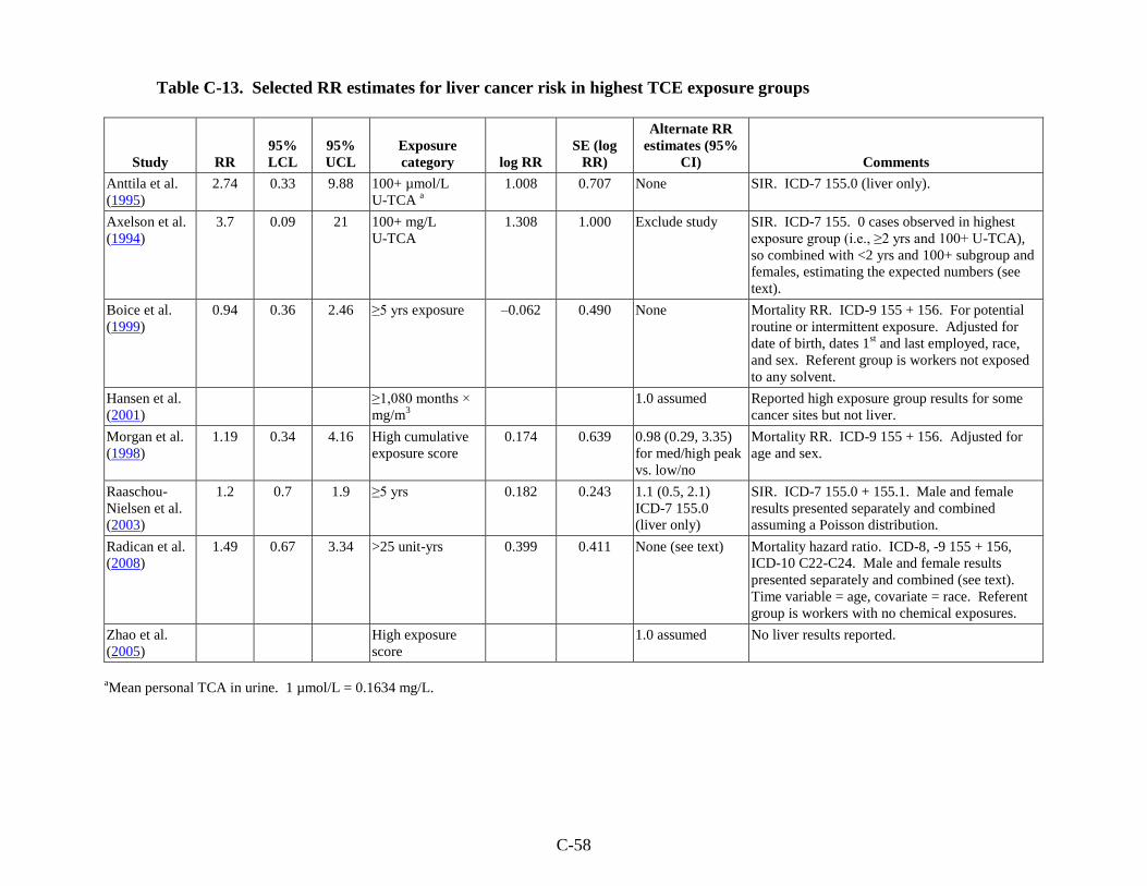
C-58
Table C-13. Selected RR estimates for liver cancer risk in highest TCE exposure groups
Study RR
95%
LCL
95%
UCL
Exposure
category log RR
SE (log
RR)
Alternate RR
estimates (95%
CI) Comments
Anttila et al.
(1995)
2.74 0.33 9.88 100+ µmol/L
U-TCA a
1.008 0.707 None SIR. ICD-7 155.0 (liver only).
Axelson et al.
(1994)
3.7 0.09 21 100+ mg/L
U-TCA
1.308 1.000 Exclude study SIR. ICD-7 155. 0 cases observed in highest
exposure group (i.e., ≥2 yrs and 100+ U-TCA),
so combined with <2 yrs and 100+ subgroup and
females, estimating the expected numbers (see
text).
Boice et al.
(1999)
0.94 0.36 2.46 ≥5 yrs exposure –0.062 0.490 None Mortality RR. ICD-9 155 + 156. For potential
routine or intermittent exposure. Adjusted for
date of birth, dates 1st and last employed, race,
and sex. Referent group is workers not exposed
to any solvent.
Hansen et al.
(2001)
≥1,080 months ×
mg/m3
1.0 assumed Reported high exposure group results for some
cancer sites but not liver.
Morgan et al.
(1998)
1.19 0.34 4.16 High cumulative
exposure score
0.174 0.639 0.98 (0.29, 3.35)
for med/high peak
vs. low/no
Mortality RR. ICD-9 155 + 156. Adjusted for
age and sex.
Raaschou-
Nielsen et al.
(2003)
1.2 0.7 1.9 ≥5 yrs 0.182 0.243 1.1 (0.5, 2.1)
ICD-7 155.0
(liver only)
SIR. ICD-7 155.0 + 155.1. Male and female
results presented separately and combined
assuming a Poisson distribution.
Radican et al.
(2008)
1.49 0.67 3.34 >25 unit-yrs 0.399 0.411 None (see text) Mortality hazard ratio. ICD-8, -9 155 + 156,
ICD-10 C22-C24. Male and female results
presented separately and combined (see text).
Time variable = age, covariate = race. Referent
group is workers with no chemical exposures.
Zhao et al.
(2005)
High exposure
score
1.0 assumed No liver results reported.
aMean personal TCA in urine. 1 µmol/L = 0.1634 mg/L.
C-59
For Axelson et al. (1994), there were no liver cancer cases in the highest exposure group
(≥2 years and 100+ mean U-TCA level), so no log RR and SE (log RR) estimates were available
for the meta-analysis. Instead, the <2 and ≥2 years results were combined, assuming expected
numbers of cases were proportional to person-years, and 100+ U-TCA (with any exposure
duration) was used as the highest exposure category. The female contribution to the expected
number was also estimated, again assuming proportionality to person-years, and adjusting for the
difference between female and male age-adjusted liver cancer incidence rates. The estimated RR
and SE values for the combined exposure times and sexes were used in the primary analysis. In
an alternate analysis, the Axelson et al. (1994) study was excluded altogether, because we
estimated that <0.2 cases were expected in the highest exposure category, suggesting that the
study had low power to detect an effect in the highest exposure group and would contribute little
weight to the meta-analysis.
For Boice et al. (1999), only results for workers with ―any potential exposure‖ were
presented by exposure category, and the referent group is workers not exposed to any solvent.
For Morgan et al. (1998), the primary analysis used results for the cumulative exposure metric,
and a sensitivity analysis was done with the results for the peak exposure metric. For Raaschou-
Nielsen et al. (2003), unlike for NHL and RCC, liver cancer results for the subcohort with
expected higher exposure levels were not presented, so the only highest-exposure-group results
were for duration of employment in the total cohort. Results for cancers of the liver and gall
bladder/biliary passages combined were used for the primary analysis and results for liver cancer
alone in a sensitivity analysis.
For Radican et al. (2008), it should be noted that the referent group is workers with no
chemical exposures, not just no TCE exposure. Furthermore, results for exposure groups (based
on cumulative exposure scores) were reported separately for males and females and were
combined for this assessment using inverse-variance weighting, as in a fixed-effect meta-
analysis. In addition to results for biliary passage and liver cancer combined, Radican et al.
(2008) present results for liver only by exposure group; however, there were no liver cancer
deaths in females and the number expected was not reported, so no alternate analysis for the
highest exposure groups with an RR estimate from Radican et al. (2008) for liver cancer only
was conducted. Radican et al. (2008) present only mortality hazard ratio estimates by exposure
group; however, in an earlier follow-up of this same cohort, Blair et al. (1998) present both
incidence and mortality RR estimates by exposure group. As with the Radican et al. (2008) liver
cancer only results, however, there were no incident cases for females in the highest exposure
group in Blair et al. (1998) (and the expected number was not reported). Additionally, there
were more biliary passage/liver cancer deaths (31) in Radican et al. (2008) than incident cases
(13) in Blair et al. (1998) overall and in the highest exposure group (14 vs. 4). Thus, we elected
to use only the Radican et al. (2008) mortality results from this cohort and not to include an
alternate analysis based on incidence results from the earlier follow-up. Radican et al. (2008)
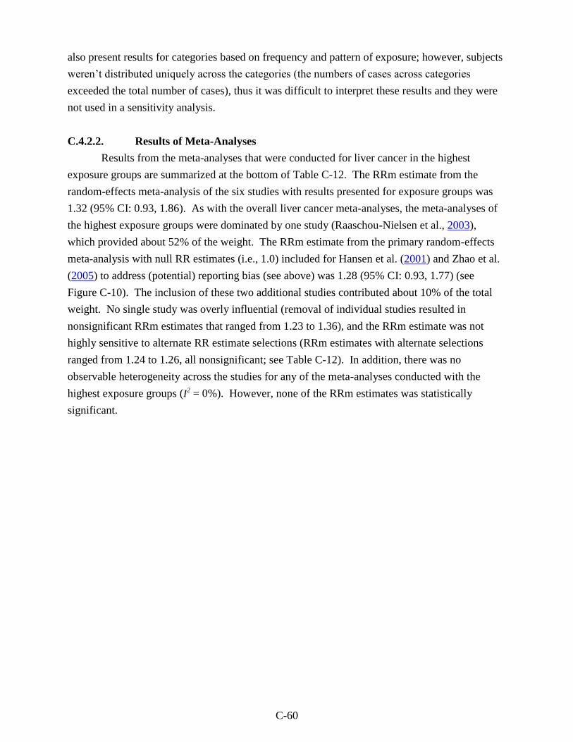
C-60
also present results for categories based on frequency and pattern of exposure; however, subjects
weren‘t distributed uniquely across the categories (the numbers of cases across categories
exceeded the total number of cases), thus it was difficult to interpret these results and they were
not used in a sensitivity analysis.
C.4.2.2. Results of Meta-Analyses
Results from the meta-analyses that were conducted for liver cancer in the highest
exposure groups are summarized at the bottom of Table C-12. The RRm estimate from the
random-effects meta-analysis of the six studies with results presented for exposure groups was
1.32 (95% CI: 0.93, 1.86). As with the overall liver cancer meta-analyses, the meta-analyses of
the highest exposure groups were dominated by one study (Raaschou-Nielsen et al., 2003),
which provided about 52% of the weight. The RRm estimate from the primary random-effects
meta-analysis with null RR estimates (i.e., 1.0) included for Hansen et al. (2001) and Zhao et al.
(2005) to address (potential) reporting bias (see above) was 1.28 (95% CI: 0.93, 1.77) (see
Figure C-10). The inclusion of these two additional studies contributed about 10% of the total
weight. No single study was overly influential (removal of individual studies resulted in
nonsignificant RRm estimates that ranged from 1.23 to 1.36), and the RRm estimate was not
highly sensitive to alternate RR estimate selections (RRm estimates with alternate selections
ranged from 1.24 to 1.26, all nonsignificant; see Table C-12). In addition, there was no
observable heterogeneity across the studies for any of the meta-analyses conducted with the
highest exposure groups (I2 = 0%). However, none of the RRm estimates was statistically
significant.
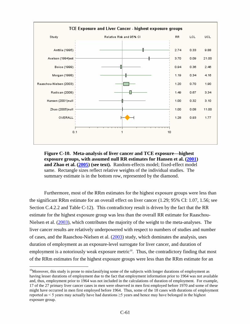
C-61
Figure C-10. Meta-analysis of liver cancer and TCE exposure—highest
exposure groups, with assumed null RR estimates for Hansen et al. (2001)
and Zhao et al. (2005) (see text). Random-effects model; fixed-effect model
same. Rectangle sizes reflect relative weights of the individual studies. The
summary estimate is in the bottom row, represented by the diamond.
Furthermore, most of the RRm estimates for the highest exposure groups were less than
the significant RRm estimate for an overall effect on liver cancer (1.29; 95% CI: 1.07, 1.56; see
Section C.4.2.2 and Table C-12). This contradictory result is driven by the fact that the RR
estimate for the highest exposure group was less than the overall RR estimate for Raaschou-
Nielsen et al. (2003), which contributes the majority of the weight to the meta-analyses. The
liver cancer results are relatively underpowered with respect to numbers of studies and number
of cases, and the Raaschou-Nielsen et al. (2003) study, which dominates the analysis, uses
duration of employment as an exposure-level surrogate for liver cancer, and duration of
employment is a notoriously weak exposure metric10. Thus, the contradictory finding that most
of the RRm estimates for the highest exposure groups were less than the RRm estimate for an
10
Moreover, this study is prone to misclassifying some of the subjects with longer durations of employment as
having lesser durations of employment due to the fact that employment information prior to 1964 was not available
and, thus, employment prior to 1964 was not included in the calculations of duration of employment. For example,
17 of the 27 primary liver cancer cases in men were observed in men first employed before 1970 and some of these
might have occurred in men first employed before 1964. Thus, some of the 18 cases with durations of employment
reported as < 5 years may actually have had durations ≥5 years and hence may have belonged in the highest
exposure group.
C-62
overall effect does not rule out an effect of TCE on liver cancer; however, it certainly does not
provide additional support for such an effect.
C.4.3. Discussion of Liver Cancer Meta-Analysis Results
For the most part, the meta-analyses of the overall effect of TCE exposure on liver (and
gall bladder/biliary passages) cancer suggest a small, statistically significant increase in risk.
The summary estimate from the primary random-effects meta-analysis of the nine (all cohort)
studies was 1.29 (95% CI: 1.07, 1.56). The analysis was dominated by one large study that
contributed about 53% of the weight. When this study was removed, the RRm estimate
decreased somewhat and was no longer statistically significant (RRm = 1.22; 95% CI: 0.93,
1.61). The summary estimate was not overly influenced by any other single study, nor was it
overly sensitive to individual RR estimate selections. The next largest downward impacts were
from the removal of the Anttila et al. (1995) study, resulting in an RRm estimate of 1.24
(95% CI: 1.02, 1.51), and from the substitution of the Morgan et al. (1998) unpublished RR
estimate (EHS, 1997) with the published SMR estimate (Morgan et al., 1998), resulting in an
RRm estimate of 1.26 (95% CI: 1.05, 1.52). Substituting the RR estimates for liver/gall
bladder/biliary passage cancers with those of liver cancer alone for the three studies that
provided these results yielded an RRm estimate of 1.25 (95% CI: 0.99, 1.57). There was no
evidence of publication bias in this data set, and there was no observable heterogeneity across the
study results.
Six of the nine studies provided liver cancer results by exposure level. Two other studies
reported results for other cancer sites by exposure level, but not liver cancer; thus, to address this
reporting bias, null values (i.e., RR estimates of 1.0) were used for these studies. Different
exposure metrics were used in the various studies, and the purpose of combining results across
the different highest exposure groups was not to estimate an RRm associated with some level of
exposure, but rather to see the impacts of combining RR estimates that should be less affected by
exposure misclassification. In other words, the highest exposure category is more likely to
represent a greater differential TCE exposure compared to people in the referent group than the
exposure differential for the overall (typically any vs. none) exposure comparison. Thus, if TCE
exposure increases the risk of liver cancer, the effects should be more apparent in the highest
exposure groups. However, the RRm estimate from the primary meta-analysis of the highest
exposure group results (and most of the RRm estimates from the sensitivity analyses) was less
than the RRm estimate from the overall exposure analysis. This anomalous result is driven by
the fact that for Raaschou-Nielsen et al. (2003), which contributes the majority of the weight to
the meta-analyses, the RR estimate for the highest exposure group, although >1, was less than
the overall RR estimate.
Thus, while there is the suggestion of an increased risk for liver cancer associated with
TCE exposure, the statistical significance of the overall summary estimate is dependent on one
C-63
study, which provides the majority of the weight in the meta-analyses. Removal of this study
yields an RRm estimate that is decreased somewhat but is still >1; however, it becomes
nonsignificant (p = 0.15). Furthermore, meta-analysis results for the highest exposure groups
yielded generally lower RRm estimates than for an overall effect. These results do not rule out
an effect of TCE on liver cancer, because the liver cancer results are relatively underpowered
with respect to numbers of studies and number of cases and the overwhelming study in terms of
weight uses the weak exposure surrogate of duration of employment for categorizing exposure
level; however, at present, there is only modest support for such an effect.
C.5. META-ANALYSIS FOR LUNG CANCER
C.5.1. Overall Effect of TCE Exposure
C.5.1.1. Selection of RR Estimates
Although there was no general indication of an increased risk of lung cancer associated
with TCE exposure in the epidemiologic literature, the Science Advisory Board recommended a
meta-analysis for lung cancer to more exhaustively examine the issue of smoking as a possible
confounder in the kidney cancer studies (SAB, 2011). Only the cohort studies were considered
for the meta-analysis because these provide a consistent group of studies to compare RRm
estimates for kidney cancer to those for lung cancer and the cohort studies are the studies of
concern for potential confounding since the kidney cancer results from these studies were not
adjusted for smoking. The selected RR estimates for lung cancer from the nine cohort studies
are presented in Table C-14. All of the studies, with the possible exception of Greenland et al.
(1994), reported cancers of the lung and bronchus combined. Some also included cancer of the
trachea; however, this is a rare tumor (<0.1% of tumors) (Macchiarini, 2006) and so its inclusion
is negligible.
As for NHL and kidney and liver cancer, many of the studies provided RR estimates only
for males and females combined, and we are not aware of any basis for a sex difference in the
effects of TCE on lung cancer risk; thus, wherever possible, RR estimates for males and females
combined were used. The only two studies of much size (in terms of number of lung cancer
cases) that provided results separately by sex were Raaschou-Nielsen et al. (2003) and Radican
et al. (2008). The results from Raaschou-Nielsen et al. (2003) suggest that lung cancer RR in
females might be slightly higher than the RR in males (SIR: males 1.4 [95% CI: 1.3, 1.5;
559 cases], females 1.9 [95% CI: 1.5, 2.4; 73 cases]), but the difference narrows when a 20-year
lag is taken into account (males 1.4 [95% CI: 1.2, 1.6; 202 cases], females 1.6 [95% CI: 1.0, 2.3;
26 cases]). Radican et al. (2008) report hazard ratios for lung cancer of 0.91 (95% CI: 0.67,
1.24; 155 deaths) for males and 0.53 (95% CI: 0.27, 1.07; 11 deaths) for females, but these
results are based on fewer cases, especially in females.
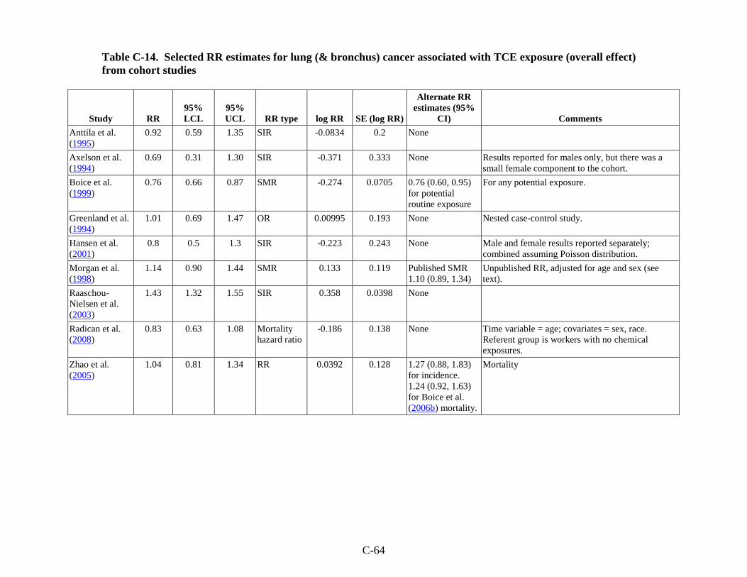
C-64
Table C-14. Selected RR estimates for lung (& bronchus) cancer associated with TCE exposure (overall effect)
from cohort studies
Study RR
95%
LCL
95%
UCL RR type log RR SE (log RR)
Alternate RR
estimates (95%
CI) Comments
Anttila et al.
(1995)
0.92 0.59 1.35 SIR -0.0834 0.2 None
Axelson et al.
(1994)
0.69 0.31 1.30 SIR -0.371 0.333 None Results reported for males only, but there was a
small female component to the cohort.
Boice et al.
(1999)
0.76 0.66 0.87 SMR -0.274 0.0705 0.76 (0.60, 0.95)
for potential
routine exposure
For any potential exposure.
Greenland et al.
(1994)
1.01 0.69 1.47 OR 0.00995 0.193 None Nested case-control study.
Hansen et al.
(2001)
0.8 0.5 1.3 SIR -0.223 0.243 None Male and female results reported separately;
combined assuming Poisson distribution.
Morgan et al.
(1998)
1.14 0.90 1.44 SMR 0.133 0.119 Published SMR
1.10 (0.89, 1.34)
Unpublished RR, adjusted for age and sex (see
text).
Raaschou-
Nielsen et al.
(2003)
1.43 1.32 1.55 SIR 0.358 0.0398 None
Radican et al.
(2008)
0.83 0.63 1.08 Mortality
hazard ratio
-0.186 0.138 None Time variable = age; covariates = sex, race.
Referent group is workers with no chemical
exposures.
Zhao et al.
(2005)
1.04 0.81 1.34 RR 0.0392 0.128 1.27 (0.88, 1.83)
for incidence.
1.24 (0.92, 1.63)
for Boice et al.
(2006b) mortality.
Mortality
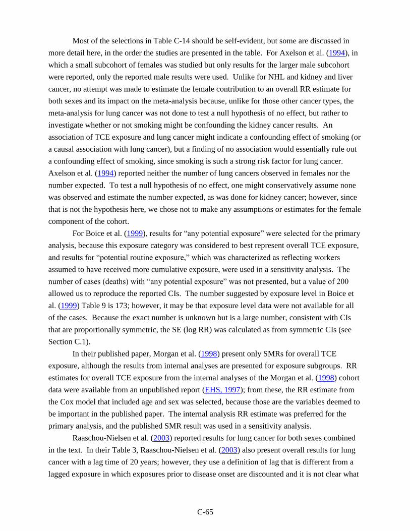
C-65
Most of the selections in Table C-14 should be self-evident, but some are discussed in
more detail here, in the order the studies are presented in the table. For Axelson et al. (1994), in
which a small subcohort of females was studied but only results for the larger male subcohort
were reported, only the reported male results were used. Unlike for NHL and kidney and liver
cancer, no attempt was made to estimate the female contribution to an overall RR estimate for
both sexes and its impact on the meta-analysis because, unlike for those other cancer types, the
meta-analysis for lung cancer was not done to test a null hypothesis of no effect, but rather to
investigate whether or not smoking might be confounding the kidney cancer results. An
association of TCE exposure and lung cancer might indicate a confounding effect of smoking (or
a causal association with lung cancer), but a finding of no association would essentially rule out
a confounding effect of smoking, since smoking is such a strong risk factor for lung cancer.
Axelson et al. (1994) reported neither the number of lung cancers observed in females nor the
number expected. To test a null hypothesis of no effect, one might conservatively assume none
was observed and estimate the number expected, as was done for kidney cancer; however, since
that is not the hypothesis here, we chose not to make any assumptions or estimates for the female
component of the cohort.
For Boice et al. (1999), results for ―any potential exposure‖ were selected for the primary
analysis, because this exposure category was considered to best represent overall TCE exposure,
and results for ―potential routine exposure,‖ which was characterized as reflecting workers
assumed to have received more cumulative exposure, were used in a sensitivity analysis. The
number of cases (deaths) with ―any potential exposure‖ was not presented, but a value of 200
allowed us to reproduce the reported CIs. The number suggested by exposure level in Boice et
al. (1999) Table 9 is 173; however, it may be that exposure level data were not available for all
of the cases. Because the exact number is unknown but is a large number, consistent with CIs
that are proportionally symmetric, the SE (log RR) was calculated as from symmetric CIs (see
Section C.1).
In their published paper, Morgan et al. (1998) present only SMRs for overall TCE
exposure, although the results from internal analyses are presented for exposure subgroups. RR
estimates for overall TCE exposure from the internal analyses of the Morgan et al. (1998) cohort
data were available from an unpublished report (EHS, 1997); from these, the RR estimate from
the Cox model that included age and sex was selected, because those are the variables deemed to
be important in the published paper. The internal analysis RR estimate was preferred for the
primary analysis, and the published SMR result was used in a sensitivity analysis.
Raaschou-Nielsen et al. (2003) reported results for lung cancer for both sexes combined
in the text. In their Table 3, Raaschou-Nielsen et al. (2003) also present overall results for lung
cancer with a lag time of 20 years; however, they use a definition of lag that is different from a
lagged exposure in which exposures prior to disease onset are discounted and it is not clear what
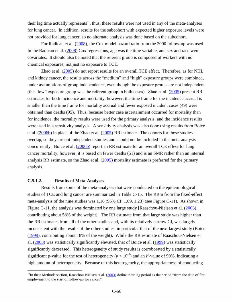
C-66
their lag time actually represents11, thus, these results were not used in any of the meta-analyses
for lung cancer. In addition, results for the subcohort with expected higher exposure levels were
not provided for lung cancer, so no alternate analysis was done based on the subcohort.
For Radican et al. (2008), the Cox model hazard ratio from the 2000 follow-up was used.
In the Radican et al. (2008) Cox regressions, age was the time variable, and sex and race were
covariates. It should also be noted that the referent group is composed of workers with no
chemical exposures, not just no exposure to TCE.
Zhao et al. (2005) do not report results for an overall TCE effect. Therefore, as for NHL
and kidney cancer, the results across the ―medium‖ and ―high‖ exposure groups were combined,
under assumptions of group independence, even though the exposure groups are not independent
(the ―low‖ exposure group was the referent group in both cases). Zhao et al. (2005) present RR
estimates for both incidence and mortality; however, the time frame for the incidence accrual is
smaller than the time frame for mortality accrual and fewer exposed incident cases (49) were
obtained than deaths (95). Thus, because better case ascertainment occurred for mortality than
for incidence, the mortality results were used for the primary analysis, and the incidence results
were used in a sensitivity analysis. A sensitivity analysis was also done using results from Boice
et al. (2006b) in place of the Zhao et al. (2005) RR estimate. The cohorts for these studies
overlap, so they are not independent studies and should not be included in the meta-analysis
concurrently. Boice et al. (2006b) report an RR estimate for an overall TCE effect for lung
cancer mortality; however, it is based on fewer deaths (51) and is an SMR rather than an internal
analysis RR estimate, so the Zhao et al. (2005) mortality estimate is preferred for the primary
analysis.
C.5.1.2. Results of Meta-Analyses
Results from some of the meta-analyses that were conducted on the epidemiological
studies of TCE and lung cancer are summarized in Table C-15. The RRm from the fixed-effect
meta-analysis of the nine studies was 1.16 (95% CI: 1.09, 1.23) (see Figure C-11). As shown in
Figure C-11, the analysis was dominated by one large study [Raaschou-Nielsen et al. (2003),
contributing about 58% of the weight]. The RR estimate from that large study was higher than
the RR estimates from all of the other studies and, with its relatively narrow CI, was largely
inconsistent with the results of the other studies, in particular that of the next largest study (Boice
(1999), contributing about 18% of the weight). While the RR estimate of Raaschou-Nielsen et
al. (2003) was statistically significantly elevated, that of Boice et al. (1999) was statistically
significantly decreased. This heterogeneity of study results is corroborated by a statistically
significant p-value for the test of heterogeneity (p < 10-8
) and an I2-value of 90%, indicating a
high amount of heterogeneity. Because of this heterogeneity, the appropriateness of conducting
11
In their Methods section, Raaschou-Nielsen et al. (2003) define their lag period as the period ―from the date of first
employment to the start of follow-up for cancer‖.
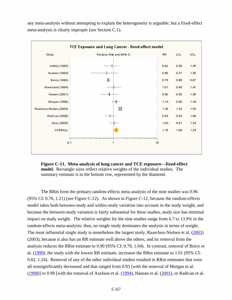
C-67
any meta-analysis without attempting to explain the heterogeneity is arguable, but a fixed-effect
meta-analysis is clearly improper (see Section C.1).
Figure C-11. Meta-analysis of lung cancer and TCE exposure—fixed-effect
model. Rectangle sizes reflect relative weights of the individual studies. The
summary estimate is in the bottom row, represented by the diamond.
The RRm from the primary random-effects meta-analysis of the nine studies was 0.96
(95% CI: 0.76, 1.21) (see Figure C-12). As shown in Figure C-12, because the random-effects
model takes both between-study and within-study variation into account in the study weight, and
because the between-study variation is fairly substantial for these studies, study size has minimal
impact on study weight. The relative weights for the nine studies range from 6.7 to 13.9% in the
random-effects meta-analysis; thus, no single study dominates the analysis in terms of weight.
The most influential single study is nonetheless the largest study, Raaschou-Nielsen et al. (2003)
(2003), because it also has an RR estimate well above the others, and its removal from the
analysis reduces the RRm estimate to 0.90 (95% CI: 0.79, 1.04). In contrast, removal of Boice et
al. (1999), the study with the lowest RR estimate, increases the RRm estimate to 1.01 (95% CI:
0.82, 1.24). Removal of any of the other individual studies resulted in RRm estimates that were
all nonsignificantly decreased and that ranged from 0.93 [with the removal of Morgan et al.
(1998)] to 0.98 [with the removal of Axelson et al. (1994), Hansen et al. (2001), or Radican et al.
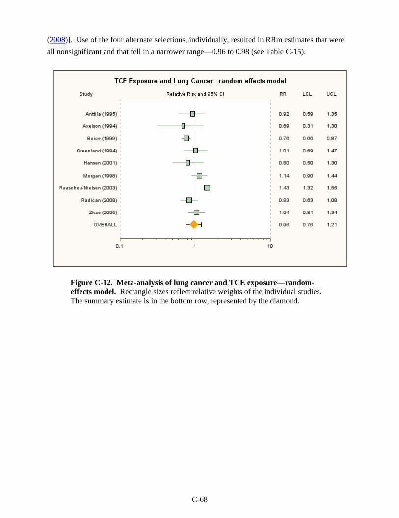
C-68
(2008)]. Use of the four alternate selections, individually, resulted in RRm estimates that were
all nonsignificant and that fell in a narrower range—0.96 to 0.98 (see Table C-15).
Figure C-12. Meta-analysis of lung cancer and TCE exposure—random-
effects model. Rectangle sizes reflect relative weights of the individual studies.
The summary estimate is in the bottom row, represented by the diamond.
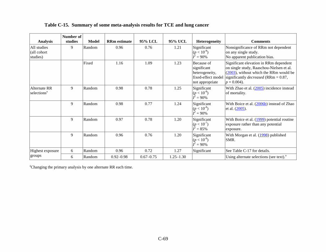
C-69
Table C-15. Summary of some meta-analysis results for TCE and lung cancer
Analysis
Number of
studies Model RRm estimate 95% LCL 95% UCL Heterogeneity Comments
All studies
(all cohort
studies)
9 Random 0.96 0.76 1.21 Significant
(p < 10-8
)
I2 = 90%
Nonsignificance of RRm not dependent
on any single study.
No apparent publication bias.
Fixed 1.16 1.09 1.23 Because of
significant
heterogeneity,
fixed-effect model
not appropriate
Significant elevation in RRm dependent
on single study, Raaschou-Nielsen et al.
(2003), without which the RRm would be
significantly decreased (RRm = 0.87,
p = 0.004).
Alternate RR
selectionsa
9 Random 0.98 0.78 1.25 Significant
(p < 10-8
)
I2 = 90%
With Zhao et al. (2005) incidence instead
of mortality.
9 Random 0.98 0.77 1.24 Significant
(p < 10-8
)
I2 = 90%
With Boice et al. (2006b) instead of Zhao
et al. (2005).
9 Random 0.97 0.78 1.20 Significant
(p < 10-7
)
I2 = 85%
With Boice et al. (1999) potential routine
exposure rather than any potential
exposure.
9 Random 0.96 0.76 1.20 Significant
(p < 10-8
)
I2 = 90%
With Morgan et al. (1998) published
SMR.
Highest exposure
groups
6 Random 0.96 0.72 1.27 Significant See Table C-17 for details.
6 Random 0.92–0.98 0.67–0.75 1.25–1.30 Using alternate selections (see text).a
aChanging the primary analysis by one alternate RR each time.
C-70
As discussed above, there was significant heterogeneity across the nine studies. All of
the lung cancer studies were cohort studies, so no subgroup analyses examining cohort and case-
control studies separately, as was done for NHL and kidney cancer, were conducted. In addition,
no alternate quantitative investigations of heterogeneity were pursued because our goal here was
to investigate lung cancer risks as an indication of possible confounding of the kidney cancer
results by smoking, not to do an all-encompassing meta-analysis of lung cancer. The majority of
the studies have nonsignificant RR estimates for lung cancer that fall near or <1. The relative
outliers are the significantly increased RR estimate from Raaschou-Nielsen et al. (2003) and the
significantly decreased RR estimate from Boice et al. (1999). The Raaschou-Nielsen et al.
(2003) study considered a lot of different job titles and the RR estimate could reflect a TCE
effect or exposure to other chemicals that are lung carcinogens. Alternatively, because the study
is an SMR study of largely blue-collar workers and the comparison population is the general
Danish population, the elevated RR estimate could reflect small differences in smoking rates
between those two populations. However, if the observed increase is attributable to smoking, it‘s
not enough of an effect to explain the increased RR estimate for RCC in the same study because
smoking is a much stronger risk factor for lung cancer than for RCC, whereas the increased RR
estimate for lung cancer in the study was relatively small (Raaschou-Nielsen et al., 2003); see
also Section 4.4.2.3). It is unclear why the Boice et al. (1999) study reports a significantly
decreased RR estimate. In any event, there is no increase in the RRm estimate for all nine
studies from the random-effects model, suggesting that there is no confounding of the overall
RRm for kidney cancer by smoking, in particular for the cohort studies.
As discussed in Section C.1, publication bias was examined in several different ways, and
there is no indication of publication bias for these lung cancer studies (results not shown). If
anything, the relationship between study size and RR estimate is the opposite of what would be
expected if publication bias were occurring because the one large study is the only study with a
significantly increased RR estimate and incorporating studies with increasing SE one at a time,
generally shows a decrease in effect size with addition of the less precise studies.
C.5.2. Lung Cancer Effect in the Highest Exposure Groups
C.5.2.1. Selection of RR Estimates
The selected RR estimates for lung cancer in the highest TCE exposure categories, for
studies that provided such estimates, are presented in Table C-16. Six of the nine cohort studies
reported lung cancer risk estimates categorized by exposure level. As in Section C.5.1.1 for the
overall risk estimates, RR estimates for males and females combined were used, wherever
possible.
Three of the nine cohort studies (Axelson et al., 1994); (Hansen et al., 2001); (Zhao et al.,
2005) did not report lung cancer risk estimates categorized by exposure level, even though these
same studies reported such estimates for selected other cancer sites. Unlike for the other cancer
C-71
types, we did not attempt to address the issue of unreported results by including RR estimates of
1 for the missing estimates. This is because, as discussed in Section C.5.1.1 above with respect
to estimate a female contribution to the Axelson et al. (1994) study, unlike for the other cancer
types, we are not testing a null hypothesis of no effect for lung cancer but rather investigating
whether smoking might be a confounder in the kidney cancer studies. Thus, we would not want
to bias the RRm estimate toward 1 in this case by including estimates of 1 for missing RR
values.
For Boice et al. (1999), only results for workers with ―any potential exposure‖ were
presented by exposure category, and the referent group is workers not exposed to any solvent.
For Morgan et al. (1998), the primary analysis used results for the cumulative exposure
metric, and a sensitivity analysis was done with the results for the peak exposure metric.
For Raaschou-Nielsen et al. (2003), unlike for NHL and RCC, lung cancer results for the
subcohort with expected higher exposure levels were not presented, so the only highest-
exposure-group results were for duration of employment in the total cohort. Results for males
and females combined were estimated assuming a Poisson distribution.
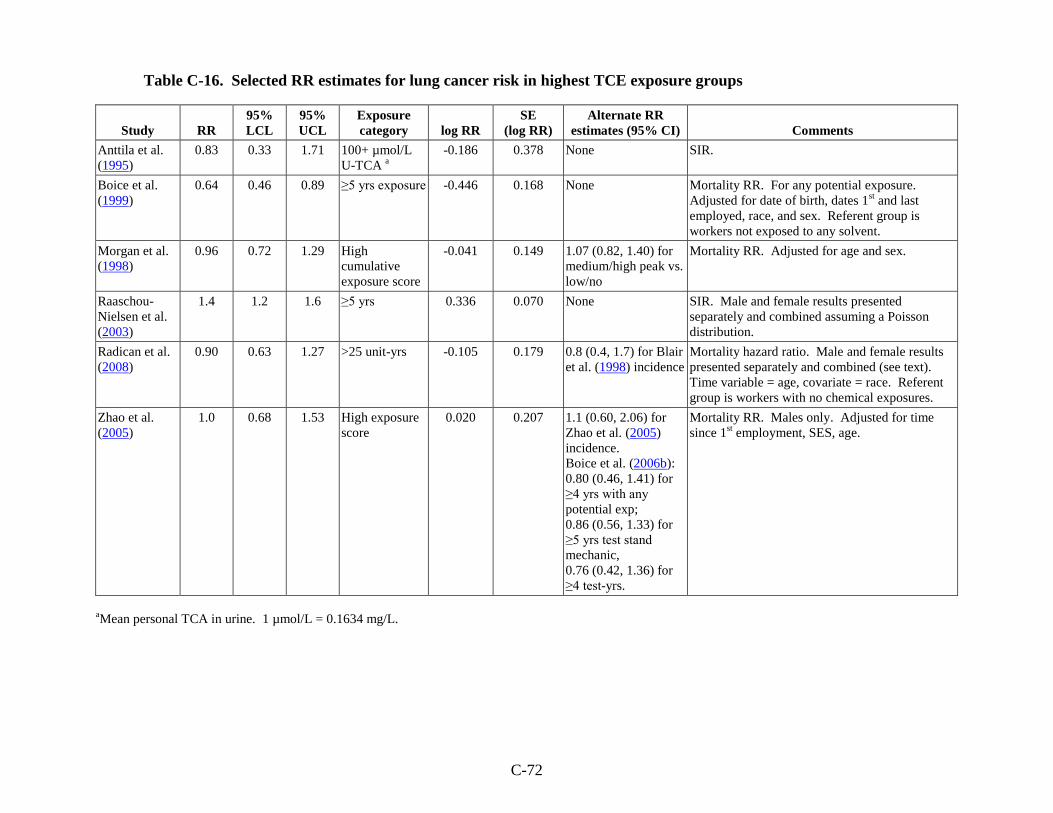
C-72
Table C-16. Selected RR estimates for lung cancer risk in highest TCE exposure groups
Study RR
95%
LCL
95%
UCL
Exposure
category log RR
SE
(log RR)
Alternate RR
estimates (95% CI) Comments
Anttila et al.
(1995)
0.83 0.33 1.71 100+ µmol/L
U-TCA a
-0.186 0.378 None SIR.
Boice et al.
(1999)
0.64 0.46 0.89 ≥5 yrs exposure -0.446 0.168 None Mortality RR. For any potential exposure.
Adjusted for date of birth, dates 1st and last
employed, race, and sex. Referent group is
workers not exposed to any solvent.
Morgan et al.
(1998)
0.96 0.72 1.29 High
cumulative
exposure score
-0.041 0.149 1.07 (0.82, 1.40) for
medium/high peak vs.
low/no
Mortality RR. Adjusted for age and sex.
Raaschou-
Nielsen et al.
(2003)
1.4 1.2 1.6 ≥5 yrs 0.336 0.070 None SIR. Male and female results presented
separately and combined assuming a Poisson
distribution.
Radican et al.
(2008)
0.90 0.63 1.27 >25 unit-yrs -0.105 0.179 0.8 (0.4, 1.7) for Blair
et al. (1998) incidence
Mortality hazard ratio. Male and female results
presented separately and combined (see text).
Time variable = age, covariate = race. Referent
group is workers with no chemical exposures.
Zhao et al.
(2005)
1.0 0.68 1.53 High exposure
score
0.020 0.207 1.1 (0.60, 2.06) for
Zhao et al. (2005)
incidence.
Boice et al. (2006b):
0.80 (0.46, 1.41) for
≥4 yrs with any
potential exp;
0.86 (0.56, 1.33) for
≥5 yrs test stand
mechanic,
0.76 (0.42, 1.36) for
≥4 test-yrs.
Mortality RR. Males only. Adjusted for time
since 1st employment, SES, age.
aMean personal TCA in urine. 1 µmol/L = 0.1634 mg/L.

C-73
For Radican et al. (2008), it should be noted that the referent group is workers with no
chemical exposures, not just no TCE exposure. Furthermore, results for exposure groups (based
on cumulative exposure scores) were reported separately for males and females and were
combined for this assessment using inverse-variance weighting, as in a fixed-effect meta-
analysis. Radican et al. (2008) present only mortality hazard ratio estimates by exposure group;
however, in an earlier follow-up of this same cohort, Blair et al. (1998) present both incidence
and mortality RR estimates by exposure group. There were no incident cases for females in the
highest exposure group in Blair et al. (1998) (and the expected number was not reported); thus,
for the same reasons we didn‘t use RR estimates of 1 for unreported RR estimates in the Axelson
et al. (1994), Hansen et al. (2001), and Zhao et al. (2005) studies discussed above, the male-only
results were used for the RR estimate without attempting to approximate a contribution to the RR
estimate from the females in the cohort. Radican et al. (2008) also present results for categories
based on frequency and pattern of exposure; however, subjects weren‘t distributed uniquely
across the categories (the numbers of cases across categories exceeded the total number of
cases); thus, it was difficult to interpret these results and they were not used in a sensitivity
analysis.
Unlike for kidney cancer, Zhao et al. (2005) present lung cancer RR estimates only for
unlagged exposures. The mortality results reflect more cases (33) in the highest exposure group
than do the incidence results (14), so the mortality RR estimate was used for the primary
analysis, and the incidence estimate was used in a sensitivity analysis. Sensitivity analyses were
also done using results from Boice et al. (2006b) in place of the Zhao et al. (2005) RR estimate.
The cohorts for these studies overlap, so they are not independent studies. Boice et al. (2006b)
report mortality RR estimates for lung cancer by years worked with any potential exposure, years
worked as a test stand mechanic, a job with potential TCE exposure, and by a measure that
weighted years with potential exposure from engine flushing by the number of flushes each year.
The Boice et al. (2006b) estimates are adjusted for years of birth and hire and for hydrazine
exposure.
C.5.2.2. Results of Meta-Analyses
Results from the meta-analyses that were conducted for lung cancer in the highest
exposure groups are summarized at the bottom of Table C-15 and reported in more detail in
Table C-17. The RRm estimate from the random-effects meta-analysis of the six studies with
results presented for exposure groups was 0.96 (95% CI: 0.72, 1.27). As with the overall results
for lung cancer, the highest-exposure-group results exhibited significant heterogeneity, with the
largest study (Raaschou-Nielsen et al., 2003) having a statistically significantly increased RR
estimate and the next largest (Boice et al., 1999) having a statistically significantly decreased RR
estimate (see Figure C-13). The remaining four studies all had nonsignificant RR estimates
closer to 1. Nonsignificance of the RRm estimate was not dependent on any single study,
C-74
although removing Raaschou-Nielsen et al. (2003) decreased the RRm estimate to 0.86 and
removing Boice et al. (1999) increased the RRm estimate to 1.07. The RRm estimate was not
highly sensitive to alternate RR estimate selections. Use of the six alternate selections,
individually, resulted in RRm estimates that were all nonsignificant and that ranged from 0.92 to
0.98 (see Table C-17). As with the primary analysis, significant heterogeneity was observed for
all of the meta-analyses with alternate selections (see Table C-17).
The RRm estimate from the primary analysis of the highest exposure groups was the
same as that for the overall TCE analysis (0.96), indicating no evidence of an exposure-response
relationship and confirming the absence of evidence of an increased risk of lung cancer
associated with TCE exposure from these studies as a whole.
C.5.3. Discussion of Lung Cancer Meta-Analysis Results
Significant heterogeneity was observed in the lung cancer results (for both overall TCE
exposure and for the highest exposure groups) from the different studies, and there was no clear
explanation for the source(s) of the heterogeneity, as discussed in Section C.5.1.2. Nonetheless,
we conducted (random-effects) meta-analyses of the lung cancer results with the goal of
addressing the question of whether or not there was evidence of an association between TCE
exposure and lung cancer that might suggest that smoking could be confounding the kidney
cancer results, in particular in the cohort studies, which did not adjust for smoking.
Both the overall and highest-exposure-group analyses yielded nonsignificant RRm
estimates of 0.96 for lung cancer. Influence analyses and sensitivity analyses using alternate RR
estimate selection for various studies similarly found no evidence of an association between TCE
exposure and lung cancer from these studies as a whole. This finding suggests that there is no
confounding of the overall RRm for kidney cancer by smoking, in particular from the cohort
studies (see Section 4.4.2.3 for a more comprehensive discussion of the issue of potential
confounding of the kidney cancer results by smoking).
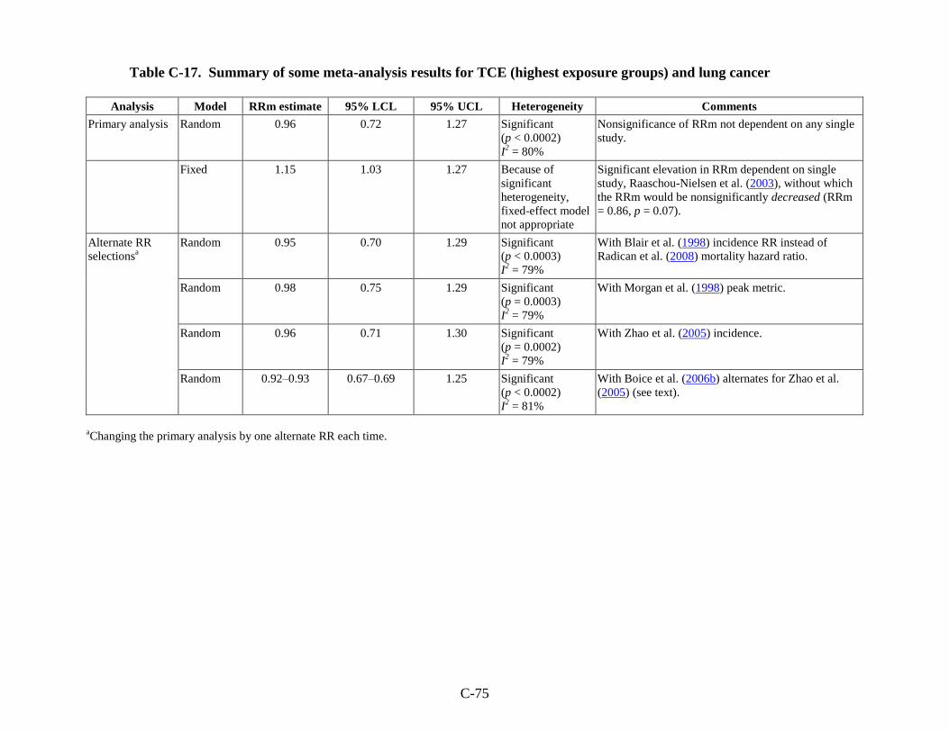
C-75
Table C-17. Summary of some meta-analysis results for TCE (highest exposure groups) and lung cancer
Analysis Model RRm estimate 95% LCL 95% UCL Heterogeneity Comments
Primary analysis Random 0.96 0.72 1.27 Significant
(p < 0.0002)
I2 = 80%
Nonsignificance of RRm not dependent on any single
study.
Fixed 1.15 1.03 1.27 Because of
significant
heterogeneity,
fixed-effect model
not appropriate
Significant elevation in RRm dependent on single
study, Raaschou-Nielsen et al. (2003), without which
the RRm would be nonsignificantly decreased (RRm
= 0.86, p = 0.07).
Alternate RR
selectionsa
Random 0.95 0.70 1.29 Significant
(p < 0.0003)
I2 = 79%
With Blair et al. (1998) incidence RR instead of
Radican et al. (2008) mortality hazard ratio.
Random 0.98 0.75 1.29 Significant
(p = 0.0003)
I2 = 79%
With Morgan et al. (1998) peak metric.
Random 0.96 0.71 1.30 Significant
(p = 0.0002)
I2 = 79%
With Zhao et al. (2005) incidence.
Random 0.92–0.93 0.67–0.69 1.25 Significant
(p < 0.0002)
I2 = 81%
With Boice et al. (2006b) alternates for Zhao et al.
(2005) (see text).
aChanging the primary analysis by one alternate RR each time.
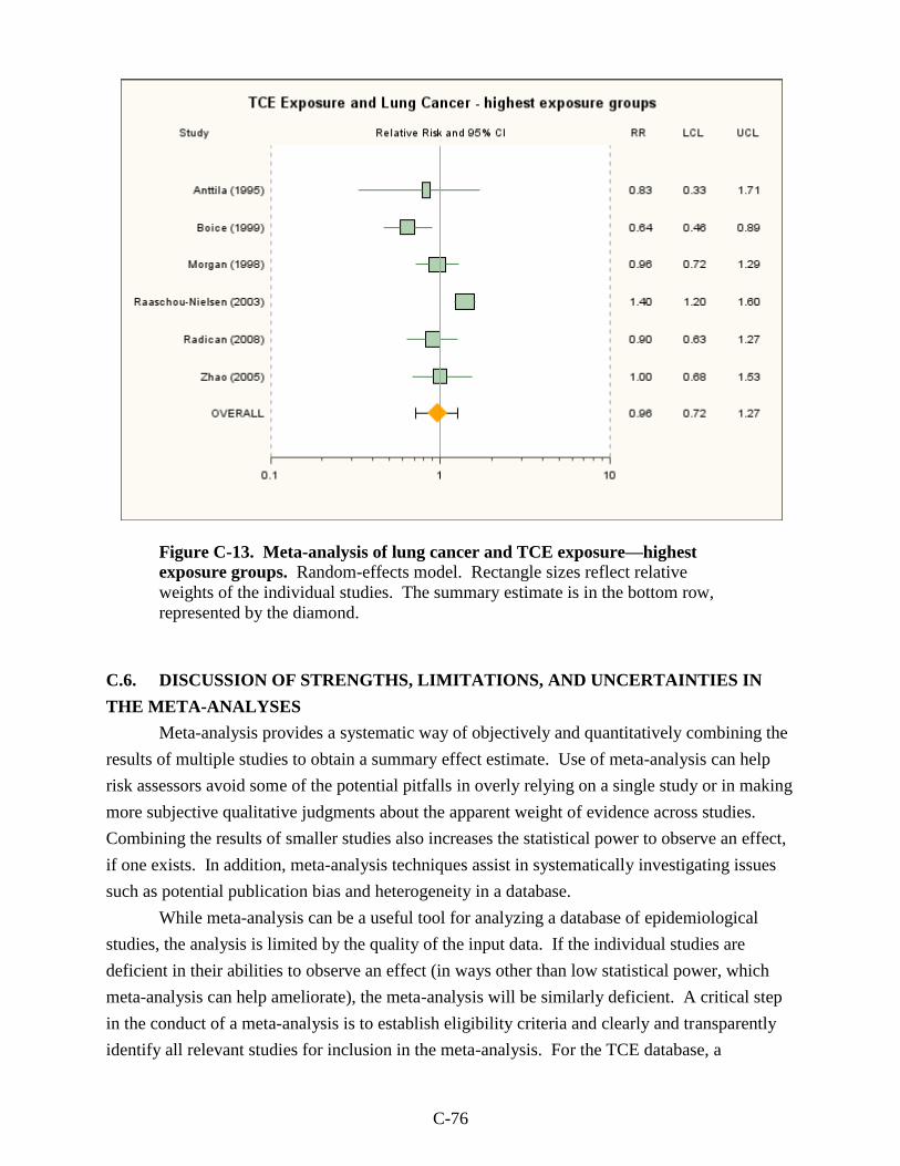
C-76
Figure C-13. Meta-analysis of lung cancer and TCE exposure—highest
exposure groups. Random-effects model. Rectangle sizes reflect relative
weights of the individual studies. The summary estimate is in the bottom row,
represented by the diamond.
C.6. DISCUSSION OF STRENGTHS, LIMITATIONS, AND UNCERTAINTIES IN
THE META-ANALYSES
Meta-analysis provides a systematic way of objectively and quantitatively combining the
results of multiple studies to obtain a summary effect estimate. Use of meta-analysis can help
risk assessors avoid some of the potential pitfalls in overly relying on a single study or in making
more subjective qualitative judgments about the apparent weight of evidence across studies.
Combining the results of smaller studies also increases the statistical power to observe an effect,
if one exists. In addition, meta-analysis techniques assist in systematically investigating issues
such as potential publication bias and heterogeneity in a database.
While meta-analysis can be a useful tool for analyzing a database of epidemiological
studies, the analysis is limited by the quality of the input data. If the individual studies are
deficient in their abilities to observe an effect (in ways other than low statistical power, which
meta-analysis can help ameliorate), the meta-analysis will be similarly deficient. A critical step
in the conduct of a meta-analysis is to establish eligibility criteria and clearly and transparently
identify all relevant studies for inclusion in the meta-analysis. For the TCE database, a
C-77
comprehensive qualitative review of available studies was conducted and eligible studies were
identified, as described in Appendix B, Section B.2.9.
Identifying all relevant studies may be hampered if publication bias has occurred.
Publication bias is a systematic error that can arise if statistically significant studies are more
likely to be published than nonsignificant studies. This can result in an upward bias on the effect
size measure (i.e., the RR estimate). To address this concern, potential publication bias was
investigated for the databases for which meta-analyses were undertaken. For the studies of
kidney cancer and liver cancer, there was no evidence of publication bias. For the studies of
NHL, there was some evidence of potential publication bias. It is uncertain whether this reflects
actual publication bias or rather an association between SE and effect size (as discussed in
Section C.1, a feature of publication bias is that smaller studies tend to have larger effect sizes)
resulting for some other reason, e.g., a difference in study populations or protocols in the smaller
studies. Furthermore, if there is publication bias in this data set, it may be creating an upward
bias on the RR estimate, but this bias does not appear to account completely for the finding of an
increased NHL risk (see Section C.2.1.2).
Another concern in meta-analyses is heterogeneity across studies. Random-effects
models were used for the primary meta-analyses in this assessment because of the diverse nature
of the individual studies. When there is no heterogeneity across the study results, the random-
effects model will give the same result as a fixed-effect model. When there is heterogeneity, the
random-effects model estimates the between-study variance. Thus, when there is heterogeneity,
the random-effects model will generate wider CIs and be more ―conservative‖ than a fixed-effect
model. However, if there is substantial heterogeneity, it may be inappropriate to combine the
studies at all. In cases of significant heterogeneity, it is important to try to investigate the
potential sources of the heterogeneity.
For the studies of kidney and liver cancer, there was no apparent heterogeneity across the
study results (i.e., random- and fixed-effects models gave identical summary estimates). For the
NHL studies, there was heterogeneity, but it was not statistically significant (p = 0.16). The
I2-value was 26%, suggesting low-to-moderate heterogeneity. When subgroup analyses were
done for the cohort and case-control studies separately, there was some heterogeneity in both
groups, but in neither case was it statistically significant. Further attempts to quantitatively
investigate the heterogeneity were not pursued because of limitations in the database. The
sources of heterogeneity are an uncertainty in the database of studies of TCE and NHL. Some
potential sources of heterogeneity, which are discussed qualitatively in Section C.2.3, include
differences in exposure assessment or in the intensity or prevalence of TCE exposures in the
study population and differences in NHL classification.
The joint occurrence of heterogeneity and potential publication bias in the database of
studies of TCE and NHL raises special concerns. Because of the heterogeneity, a random-effects
model should be used if these studies are to be combined; yet, the random-effects model gives
C-78
relatively large weight to small studies, which could exacerbate the potential impacts of
publication bias. For the NHL studies, the summary RR estimates from the random-effects and
fixed-effect models are not very different (RRm = 1.23 [95% CI: 1.07, 1.42] and 1.21 [95% CI:
1.08, 1.35], respectively); however, the CI for the fixed-effect estimate does not reflect the
between-study variance and is, thus, overly narrow.
Heterogeneity was statistically significant for the lung cancer studies (p < 10-8
) and the
I2-value was 90%, indicating that the amount of heterogeneity was high. Nonetheless, (random-
effects) meta-analyses were conducted for the purpose of investigating the potential for smoking
to be confounding the kidney cancer results (see Sections C.5 and 4.4.2.3).
C.7. CONCLUSIONS
The strongest finding from the meta-analyses was for TCE and kidney cancer. The
summary estimate from the primary random-effects meta-analysis of the 15 studies was
RRm = 1.27 (95% CI: 1.13, 1.43). There was no apparent heterogeneity across the study results
(i.e., fixed-effect model gave same summary estimate), and there was no evidence of potential
publication bias. The summary estimate was robust across influence and sensitivity analyses; the
estimate was not markedly influenced by any single study, nor was it overly sensitive to
individual RR estimate selections. The findings from the meta-analyses of the highest exposure
groups for the studies that provided kidney cancer results categorized by exposure level were
similarly robust. The summary estimate was RRm = 1.58 (95% CI: 1.28, 1.96) for the 13 studies
included in the analysis. There was no apparent heterogeneity in the highest-exposure-group
results, and the estimate was not markedly influenced by any single study, nor was it overly
sensitive to individual RR estimate selections. In sum, these robust results support a conclusion
that TCE exposure increases the risk of kidney cancer.
The meta-analyses of the overall effect of TCE exposure on NHL also suggest a small,
statistically significant increase in risk. The summary estimate from the primary random-effects
meta-analysis of the 17 studies was 1.23 (95% CI: 1.07, 1.42). This result was not overly
influenced by any single study, nor was it overly sensitive to individual RR estimate selections.
There is some evidence of potential publication bias in the NHL study data set; however, it is
uncertain that this is actually publication bias rather than an association between SE and effect
size resulting for some other reason, e.g., a difference in study populations or protocols in the
smaller studies. Furthermore, if there is publication bias, it does not appear to account
completely for the findings of an increased NHL risk. There was some heterogeneity across the
results of the 17 studies, but it was not statistically significant (p = 0.16). The I2-value was 26%,
suggesting low-to-moderate heterogeneity. The source(s) of this heterogeneity remains an
uncertainty. The summary estimate from the meta-analysis of the highest exposure groups for
the 13 studies which provided NHL results categorized by exposure level was RRm = 1.43
(95% CI: 1.13, 1.82). The statistical significance of the increased RR estimate for the highest
C-79
exposure groups was not dependent on any single study, nor was it sensitive to individual RR
estimate selections. Although there was some heterogeneity across the 13 highest-exposure-
group studies, it was not statistically significant (p = 0.30) and the I2-value was 14%, suggesting
that the amount of heterogeneity was low. Furthermore, the heterogeneity is dependent on a
single study, Cocco et al. (2010), suggesting that the RR estimate for the highest exposure group
from that study is a relative outlier. Overall, the robustness of the finding of an increased NHL
risk for the highest exposure groups strengthens the more moderate evidence from the meta-
analyses for overall effect.
The meta-analyses of the overall effect of TCE exposure on liver (and gall bladder/biliary
passages) cancer also suggest a small, statistically significant increase in risk, but the study
database is more limited. The summary estimate from the primary random-effects meta-analysis
of the nine (all cohort) studies was 1.29 (95% CI: 1.07, 1.56). The analysis was dominated by
one large study that contributed about 53% of the weight. When this study was removed, the
RRm estimate decreased somewhat and was less precise (RRm = 1.22; 95% CI: 0.93, 1.61). The
summary estimate was not overly influenced by any other single study, nor was it overly
sensitive to individual RR estimate selections. There was no evidence of publication bias in this
data set, and there was no observable heterogeneity across the study results. However, the
findings from the meta-analyses of the highest exposure groups for the studies that provided liver
cancer results categorized by exposure level do not add support to the overall effect findings.
The summary estimate was RRm = 1.28 (95% CI: 0.93, 1.77) for the eight studies included in the
analysis, which is slightly lower than the summary estimate for the overall effect. This
contradictory result is driven by the fact that the RR estimate for the highest exposure group in
the individual study which contributes the majority of the weight to the meta-analyses, although
>1, was less than the overall RR estimate for the same study. In sum, these results do not rule
out an effect of TCE on liver cancer, because the liver cancer results are relatively underpowered
with respect to numbers of studies and number of cases and the overwhelming study in terms of
weight uses the weak exposure surrogate of duration of employment for categorizing exposure
level; however, at present, there is only modest support for an increased risk of liver cancer.
Meta-analyses were also conducted for lung cancer with the goal of addressing the question of
whether or not there was evidence of an association between TCE exposure and lung cancer that
might suggest that smoking could be confounding the kidney cancer results, in particular in the
cohort studies, which did not adjust for smoking. Both the overall and highest-exposure-group
random-effects meta-analyses yielded a nonsignificant RRm estimate of 0.96 for lung cancer.
Influence analyses and sensitivity analyses using alternate RR estimate selection for various
studies similarly found no evidence of an association between TCE exposure and lung cancer
from these studies as a whole. This finding suggests that there is no confounding of the overall
RRm for kidney cancer by smoking (see Section 4.4.2.3 for a more comprehensive discussion of
the issue of potential confounding of the kidney cancer results by smoking).