TOWARDS MICROSTRUCTURE BASED TISSUE PERFUSIONRECONSTRUCTION FROM CT USING MULTISCALE MODELING

E. Rohan1, V. Lukes2, A. Jonasova2, O. Bublık2

1 NTIS, Faculty of Applied Sciences, University of West Bohemia , Pilsen, Czech Republic;(rohan@kme.zcu.cz)

2 Department of Mechanics, Faculty of Applied Sciences, University of West Bohemia ,Pilsen, Czech Republic;

Abstract. The paper deals with modeling of blood perfusion and simulation of dynamicCT investigation. The flow can be characterized at several scales for which different mod-els are used. We focus on two levels: flow in larger branching vessels is described using asimple “1D” model based of the Bernoulli equation. This model is coupled through pointsources/sinks with a “0D” model describing multicompartment flows in tissue parenchyma.We propose also a model of homogenized layer which can better reflect arrangement of themicrovessels; the homogenization approach will be used to describe flows in the parenchymaby a two-scale model which provides the effective parameters dependent on the microstruc-ture. The research is motivated by modeling liver perfusion which should enable an improvedanalysis of CT scans. For this purpose we describe a dynamic transport of the contrast fluidat levels of the “1D” and “0D” models, so that time-space distribution of the so-called tissuedensity can be computed and compared with the measured data obtained form the CT.

Keywords: Tissue perfusion, Multicompartment flow model, Porous materials, Dynamictransport equations, Homogenization.

1. Introduction

Problem of tissue perfusion reconstruction is quite challenging for the biomechanicaland biomedical research. It is desirable to find accurately parts of the tissue with an insuffi-cient blood supply, to localize anomalies in the blood micro-circulation and to quantify locallythe perfusion efficiency. Such information is need namely to asses physiological functionalityof the brain tissue and trends to pathologies. For the liver segmentation, it is important toidentify parts of the whole organ which are supplied with blood by a selected vein branch.Our effort is to improve modeling techniques for processing the standard CT investigations.

Blucher Mechanical Engineering ProceedingsMay 2014, vol. 1 , num. 1www.proceedings.blucher.com.br/evento/10wccm

Microstructurally-oriented and computationally efficient models allow for simulations of tis-sue perfusion and transport of the contrast fluid whose instantaneous volume concentration inthe parenchyma corresponds to the density registered by the CT. To cope with the complex-ity of the perfusion trees, we use a combination of 3D and 1D fluid dynamics for large andmedium vessels, respectively, whereas Darcy flow “0D” models are used to describe bloodredistribution in the parenchyma and smaller vessels. In this paper we present a simplifiedmodel where only a 1D model is employed to describe flow on the branching medium vessels.

We developed several multiscale and multicompartment models based on homoge-nization [8,10,11];they involve effective parameters computed using solutions of local ”mi-croscopic” problems in RVEs where the geometry and topology of different vessels is spec-ified; each compartment is associated with one pressure field, their local differences revealthe amount of the tissue perfusion. To describe the hierarchical arrangement of the perfusedtissue, we proposed a model of homogenized perfusion in the 3-compartment medium consti-tuted by several transversely periodic layers with dual porosities [9].Thus, a 3D volume canbe replaced by a number of 2D ”homogenized layers” coupled by conditions governing thefluid exchange between them. The 1D flow model on the branching vessel network is coupledwith the homogenized 0D flow model of the tissue perfusion by a non-compound solving pro-cedure - the sheared data (pressures and fluxes) are being exchanged between the two modelson point and line interfaces defined in the 3D domain. Once the perfusion fields are computed,the tracer redistribution can be simulated using a transport model. The local tracer concentra-tions in different compartments are averaged to obtain the density maps comparable with theCT outputs.

The paper is organized, as follows: First, in Section 2 we explain conception of a hi-erarchical flow model in the context of the liver perfusion simulation. For modeling at thewhole organ level we use a lumped model with multiple sectors and ad hoc defined perme-abilities and perfusion parameters, as discussed in Section 2.1. In Section 3 we report on thetwo-scale model of homogenized perfused layer; it is outlined how this model can be usedto describe perfusion of liver lobules at the lowermost level where the blood is transportedbetween the portal and hepatic veins. In Section 4 we describe a model of the transport of thetracer through the branching network of portal and hepatic veins

2. Hierarchical model of perfusion

The simulation of blood perfusion in tissues like liver or brain belongs to problems thatnecessitate a sort of multiscale modeling to be used, cf. [4];the term “multiscale” is employedin a slightly different manner than in [5],where the “geometrical multiscale” modeling was in-troduced in the context of the cardiovascular system. Obviously, the difficulty of the problemconsists in the nature of the flow on branching structures incorporating blood vessels of verydifferent diameters. For instance, the blood is conveyed to the liver by the portal vein with itsdiameter of D=1.3 cm. At the tissue parenchyma level, the blood channels are formed in thelobular hexagonal structures with the characteristic size of 1.5 mm, so that the sinus throughwhich the blood flows from the portal to the hepatic compartments is formed by microvesselswith the diameter of about d=10 µm. Moreover the scale change characterized by the ratiod/D = 0.001 is continuous, the perfusion trees have several hierarchies distinguished by the

number of “new” branches and reduced vessel diameters.The model which we develop should allow also for simulation of the transport of the

contrast fluid (the tracer) during the dynamic perfusion test. The aim is to provide a computa-tional feedback which would enable to analyze more accurately the CT scans obtained fromthe standard dynamic perfusion test of a patient, cf. [7].Nowadays the methods based on thedeconvolution, or maximum slope techniques provide some characteristics like the blood flow,blood volume, transition times and others for each voxel of the tissue, cf. [6].Our approachshould provide an alternative and more detailed interpretation of the measured CT scans. Theproposed strategy is based on the following tasks:

• to describe all involved hierarchies of the perfusion trees including the parenchyma bysuitable models involving few undetermined parameters;

• to reconstruct the organ (liver) shape and the blood vessels geometries up to a certainhierarchy using the image segmentation techniques (based on the CT “static” data);

• to tune (by solving some optimization problems) selected parameters of the parenchymamodel (like permeability), so that the simulated dynamic CT test is as close as possibleto the measured data.

Such a “tuned” model would enable to analyze the blood flow in particular compartments andto predict effects of intended medical treatment, like resection of a part of the tissue.

The proposed strategy contains several hurdles; on one hand the model should reflectthe microstructure and fit the complex geometry of the perfusion trees, on the other hand itshould be parameterized just using not too many parameters to prevent ill conditioning of the“tuning” step involving simulations of the steady blood flow and the dynamic tracer transport.For this purpose, the tuning parameters must reflect some important features of the perfusionsystem.

In this paper we describe a simplified model on which we test the modeling of theperfusion and tracer transport. It consists of the following parts:

1. The “inlet” and “outlet” trees which (in the case of the liver) described the portal andhepatic veins, respectively. These trees are formed by pipes and junctions representingthe branching. For simplicity we consider incompressible, inviscid steady 1D flow, asdescribed in Section 2.2.

2. The parenchyma “0D” model is constituted by equations governing a multicompartmentDarcy flow in a 3D porous medium involving a pressure field associated with eachcompartment. Thus, at any point of the organ domain Ω ⊂ R3 several (at least two)different pressure values are defined which are associated with different compartments,see Section 2.1. There are point sources and sinks defined in Ω where the “1D” treesare connected to the “0D” model. It is worth noting that our definition of a “0D” modelis different from the one used in [5]

We intend to describe the blood flow in the parenchyma using a more accurate model basedon homogenization of the tissue microstructure. In Section 3 we report on a model which canbe adapted to describe flows at the level of lobules forming a periodic structure.

2.1. Macroscopic lumped modeling of parenchyma

We approximate the perfusion at the level of tissue parenchyma using a lumped “macro-scopic” model describing parallel flows in multiple compartments, cf. [2].The model involvespressures pii, i = 1, . . . , i which must satisfy the following equations:

∇ · wi +∑

j

J ij = f i , i = 1, . . . , i in Ω ,

wi = −Ki∇pi ,

J ij = Gi

j(pi − pj) ,

(1)

where Ki is the local permeability of the i-th compartment network and Gij is the perfusion

coefficient related to compartments i, j, so that J ij describes the amount of fluid which flows

from i to j (drainage flux; obviously J ji = −J i

j ) and f i is the local source/sink flux of thei-th compartment. Equations (1) are supplemented by the non-penetration conditions,

n · wi = −n · Ki∇pi = 0 , i = 1, . . . , i . (2)

In our numerical tests we considered just two compartments, i = 2. The local source/sinkfunctions for each compartment is defined using the Dirac distributions, see (4). They estab-lish the interface between the “0D” and “1D” models, as explained below.

2.2. Flow on branching networks

Let T (J jj`ee) a branching tree formed by pipes `e and junctions J j . By J0 wedenote the input junction, whereas the terminal branches end by junctions Jk through whichthey are connected with the parenchyma. Any junction J j = e of T joins several vessels(pipes) `e, although the input and terminal junctions are just one-element sets. Further by nwe denote the number of all terminal junctions.

The simplest possible model of flow on T is presented by the following n+1 equations

1

2ρw2

0 + p0 =1

2ρw2

k + pk , k = 1, 2, . . . , n

A0w0 =n∑k

Akwk ,(3)

where (3)1 are the Bernoulli equations and (3)2 is the mass conservation; by Ak we denote thecross-sections of terminal and input branches, i.e. of the associated vessels (we use a modelwith constant cross-sections along each vessel which is a relevant simplifying assumptionwith no effect on the contrast fluid transport, as will be explained in Section 4). Now theproblem is to compute the input pressure p0 and the terminal velocities wkk, k = 1, . . . , n

for a given input velocity w0 and terminal pressures pkk.Although this model neglects the dissipation and may lead to unaccurate results in

general, in this paper we use it just for its simplicity, since the main focus is in modeling theparenchyma perfusion. Anyway, it can be extended by some energy loss terms related to thetree geometry.

2.3. Coupled “1D” – “0D” model

The “1D” model is coupled with the “0D” model through the terminal junctions whichspecify the sources and sinks f i for all the considered compartments. For the i-th compartmentsaturated by the tree T we define

f i(x) =n∑

k=1

δ(x− xk)Akwk ,

pi(xk) = pk ,

(4)

where δ(x− xk) is the Dirac distribution at point xk ∈ Ω which is associated with the terminaljunction k. Condition (4)2 couples the pressures at the terminal junctions of the “1D” modelwith the pressure fields in Ω. In practice, we use an approximation of δ(x− xk) which is basedupon the finite element discretization.

We conclude by a simple iterative algorithm used to compute the perfusion pressureand velocity fields. Since there are two trees T , as illustrated in Fig. 5, we shall label thecorresponding solutions by indices P and H, denoting quantities associated with the portaland hepatic veins. For given values wP

0 and pH0 , i.e. the velocity in the portal (inlet) vein

and the pressure in hepatic (outlet) vein, the computation proceeds by repeating the followingsteps:

1. Set all interface velocities and pressures to zero, namely pPk = 0 and wH

k = 0. Seti = 0 and τ = 1/N , for a given N ∈ N.

2. For the new iteration i := i+ 1, update wP0 := miniτ, 1wP

0 and pH0 := miniτ, 1pH

0 .

3. Solve (3) on trees T P and T H , so that(wP

0 , pPk )7→(pP

0 , wPk ), for the portal vein,

and(pH

0 , wHk )7→(wH

0 , pHk ), for the hepatic vein.

4. Solve (1)-(2) in Ω, so that(wP

k , pHk )7→(pP

k , wHk )

and (pi(x),wi(x)) is com-puted for a.a. x ∈ Ω.

5. Use the conditions (4) to update the interface variables for the next iteration i+ 1.

6. Go to step 2, unless a steady state is obtained.

3. Model of perfusion homogenized double-porous layers

Our aim is to develop a microstructurally-oriented and computationally efficient mod-eling tool which will allow for simulations of tissue perfusion. Here we focus on modellingthe tissue parenchyma. At the level of small vessels and microvessels, the perfusion can bedescribed using the Darcy flow in double porous structure consisting of 3 compartments: twomutually disconnected channels (small arteries and veins) and the matrix (microvessels andcapillaries), represented as the dual porosity, where the permeability is decreasing with thescale parameter – the size of the microstructure.

We use techniques based on the asymptotic analysis by the periodic unfolding method[3] and treat a specific microstructure topology which gives rise to several macroscopic pres-sure fields, like in [14],cf. [10], satisfying specific homogenized equations. The layer-wise

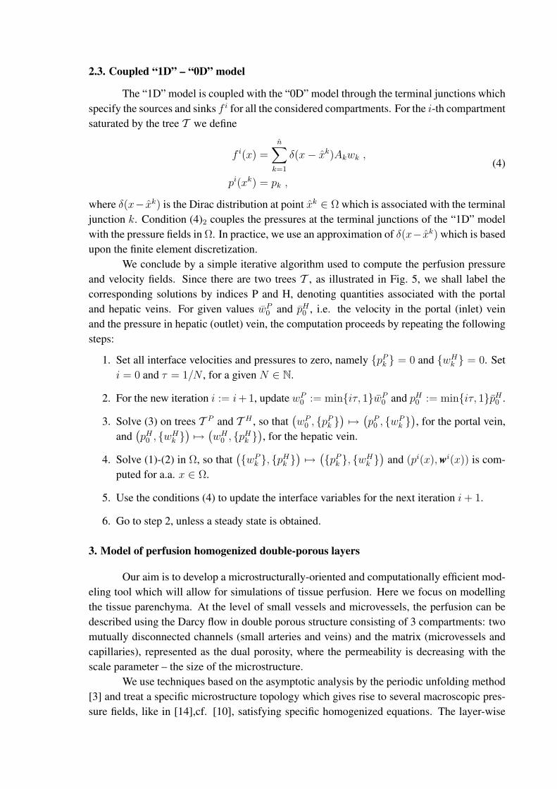
Figure 1. A periodic structure of the layer with the highlighted reference cell comprising twochannel systems A and B.

decomposition is a new feature in the context of homogenized models, up to our knowledge.A 3D layered structure occupying domain ΩH ⊂ R3 can be replaced by a finite number of 2D”homogenized layers” Γ0 ⊂ R2 coupled by conditions governing the fluid exchange betweenthem, as proposed in [12].

3.1. Macroscopic equation for single layer

The homogenized problem for pressures pA and pB, associated with two channels Aand B, describes 2D parallel flows in homogenized layer Γ0 ⊂ R2, cf. [14].Each channelsystem forms a connected domain (so, we assume at least a small co-lateralization of vesselsin the perfusion tree).

3.1.1 Microstructure and the reference cell.

The periodic microstructure is generated by the reference periodic cell, Y = Ξ × Iz,where Ξ =]0, 1[2, Iz =]− 1/2, 1/2[, with the decomposition Y = YA ∪ YB ∪ YM into 3 non-overlapping parts. Subdomains YA, YB represent the channels A and B, respectively, whereasYM represents the dual porosity (a network of capillaries). The structure is periodic w.r.t.coordinates y′ := (y1, y2) (this establishes the notion of the Y-periodicity which is refered tobelow), the transversal coordinate is denoted by z. The upper and lower boundary segments∂+Y = Ξ× z+ and ∂−Y = Ξ× z− with z± = ±1/2 are defined, whereby

∂±Y = ∂+Y ∪ ∂−Y and ∂±YD = ∂±Y ∩ ∂YD , (5)

for D = A,B,M . The channels have inlet / outlet branches entering through the layer facesΓ+ and Γ−. The inlet / outlet “surfaces” Ak

D ∈ ∂±YD are labeled with indices k ∈ JD

(obviously, AkD ∩ Al

D = δkl). For instance, in Fig. 1 each of the two depicted channels A, Bhas three such surfaces.

3.1.2 Macroscopic equations.

Two coupled “macroscopic” equations (one for A and one for B) involve the follow-ing homogenized coefficients: permeabilities (Kab)

A,B of the channels, the transmission Gand drainage (Sa)A,B,k (for channel branches k ∈ JD) coefficients. They govern the fluidredistribution between the two channel systems A and B.

Perfusion in the homogenized layer occupying the domain Γ0 is governed by twoequations, each per one channel system (in the paper the summation convention applies forindices a, b ∈ 1, 2 of the coordinates x′ = (x1, x2))

− ∂

∂xa

[KA

ab

∂

∂xb

p0,A +∑k∈JA

SA,ka gk

A

]+ G

(p0,A − p0,B

)= chAgA −FA+g+ −FA−g− in Γ0 ,

− ∂

∂xa

[KB

ab

∂

∂xb

p0,B +∑k∈JB

SB,ka gk

B

]+ G

(p0,B − p0,A

)= chB gB −FB+g+ −FB−g− in Γ0 ,

(6)

where fluxes g+/−, gD and gkD must be given such that the following solvability conditions

hold: ∑k∈JD

|AkD|gk

D = 0, D = A,B ,

∑D=A,B

∫Γ0

(1

hgD + FD+g+ + FD−g−

)= 0 .

(7)

Above FA+/−, chA are constants (the summation w.r.t. repeated indices a, b applies). Theterm G

(pA − pB

), evaluated at point x′ ∈ Γ0, expresses the amount of fluid (blood) perfused

through the matrix (the dual porosity) between sectors A and B. The details are reported in[9].

A problem involving (6) and (7) is supplemented by boundary conditions on ∂Γ0 rep-resenting the “side” boundary of the layer after the problem dimension has been reduced from3D to 2D. As the result of homogenization, the original “no-flow” (Neumann type) conditionin 3D is replaced by the following condition

naKAab

∂

∂xb

p0,A = na

∑k∈JA

SA,ka gk

A . (8)

3.1.3 Microscopic problems.

The homogenized coefficients are evaluated using the characteristic responses (alsocalled the “corrector basis functions”) which solve microscopic problems defined in subsec-tors YD, D = A,B,M of the decomposed cell Y . By ∂#Y ⊂ ∂Y we denote the “periodic”boundary of Y . There are four groups of the microscopic problems.

1st micro-problem. Find πbD (Y-periodic functions in y1, y2) such that for b = 1, 2 and

the two channels D = A,B

−∇hy · K · ∇h

y

(πb

D + yb

)= 0 in YD ,

n · K · ∇hy

(πb

D + yb

)= 0 on ∂YD \ ∂#YD ,

(9)

where K = (Kij) is the permeability in the channel D.The solution to (9) is the characteristic response of the pressure in channel YD for the

imposed “unit” pressure gradient, whereby no flow through the external boundary ∂YD\∂#YD

is admitted. Corrector functions πbD determine KD

ab, see [9].2nd micro-problem. Find pg,D (Y-periodic functions in y1, y2) such that for D = A,B

and given gkD, k ∈ JD,

−∇hy · K∇h

ypg,D = 0 in YD ,

n · K∇hyp

g,D = h−1gkD on Ak , k ∈ JD .

(10)

For solvability of (10), fluxes gkD must satisfy (7)1. Solution pg,D presents the pressure

response in channel YD to external prescribed fluxes gkD. The characteristic response to “unit”

fluxes are given by corrector functions γkD which satisfy the decomposition

pg,D =∑k∈JD

γkDg

kD , (11)

and determine coefficients SD,ka . For more details on computing γk

D and SD,ka we refer the

reader to [9].3rd micro-problem. Find ηA (Y-periodic function in y1, y2) such that

∇hy · κ∇h

yηA = 0 in YM ,

ηA = 1 on ∂YA ∩ ∂YM ,

ηA = 0 on ∂YB ∩ ∂YM ,

n · κ · ∇hyηA = 0 on ∂±YM ,

(12)

where κ = (κij) is the permeability in the dual porosity YM . Thus, for a given scale ε0, the“true” permeability is ε2

0κ.The solution of (12), i.e. the pressure in the dual porosity, is the characteristic response

to the unit pressure prescribed on walls of YA, whereas zero pressure is prescribed on walls ofYB. No flux is admitted through the external face ∂±YM . Corrector function ηA is employedto compute the homogenized coefficient G, see [9].

4th micro-problem. Find γ+/− (Y-periodic functions in y1, y2) such that

∇hy · κ∇h

yγ+/− = 0 in YM

γ+ = γ− = 0 on ∂MYA ∪ ∂MYB,

n+/− · κ∇hyγ

+/− = 1/h on ∂+/−YM ,

n−/+ · κ∇hyγ

+/− = 0 on ∂−/+YM ,

(13)

g1,εA g2,ε

A g3,εA

g1,εB g2,ε

B g3,εB

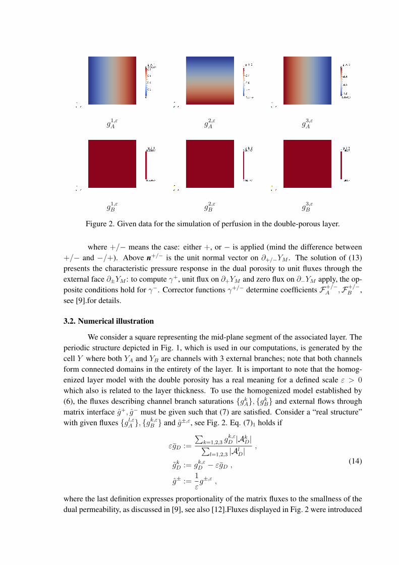
Figure 2. Given data for the simulation of perfusion in the double-porous layer.

where +/− means the case: either +, or − is applied (mind the difference between+/− and −/+). Above n+/− is the unit normal vector on ∂+/−YM . The solution of (13)presents the characteristic pressure response in the dual porosity to unit fluxes through theexternal face ∂±YM : to compute γ+, unit flux on ∂+YM and zero flux on ∂−YM apply, the op-posite conditions hold for γ−. Corrector functions γ+/− determine coefficients F+/−

A ,F+/−B ,

see [9].for details.

3.2. Numerical illustration

We consider a square representing the mid-plane segment of the associated layer. Theperiodic structure depicted in Fig. 1, which is used in our computations, is generated by thecell Y where both YA and YB are channels with 3 external branches; note that both channelsform connected domains in the entirety of the layer. It is important to note that the homog-enized layer model with the double porosity has a real meaning for a defined scale ε > 0

which also is related to the layer thickness. To use the homogenized model established by(6), the fluxes describing channel branch saturations gk

A, gkB and external flows through

matrix interface g+, g− must be given such that (7) are satisfied. Consider a “real structure”with given fluxes gl,ε

A , gk,εB and g±,ε, see Fig. 2. Eq. (7)1 holds if

εgD :=

∑k=1,2,3 g

k,εD |Ak

D|∑l=1,2,3 |Al

D|,

gkD := gk,ε

D − εgD ,

g± :=1

εg±,ε ,

(14)

where the last definition expresses proportionality of the matrix fluxes to the smallness of thedual permeability, as discussed in [9], see also [12].Fluxes displayed in Fig. 2 were introduced

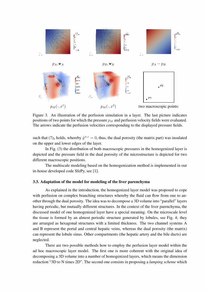
pA,wA pB,wB pA − pB

pM(·, x1) pM(·, x2) two macroscopic points:

Figure 3. An illustration of the perfusion simulation in a layer. The last picture indicatespositions of two points for which the pressure pM and perfusion velocity fields were evaluated.The arrows indicate the perfusion velocities corresponding to the displayed pressure fields.

such that (7)2 holds, whereby g±,ε = 0, thus, the dual porosity (the matrix part) was insulatedon the upper and lower edges of the layer.

In Fig. (3) the distribution of both macroscopic pressures in the homogenized layer isdepicted and the pressure field in the dual porosity of the microstructure is depicted for twodifferent macroscopic positions.

The multiscale modeling based on the homogenization method is implemented in ourin-house developed code SfePy, see [1].

3.3. Adaptation of the model for modeling of the liver parenchyma

As explained in the introduction, the homogenized layer model was proposed to copewith perfusion on complex branching structures whereby the fluid can flow from one to an-other through the dual porosity. The idea was to decompose a 3D volume into “parallel” layershaving periodic, but mutually different structures. In the context of the liver parenchyma, thediscussed model of one homogenized layer have a special meaning. On the microscale levelthe tissue is formed by an almost periodic structure generated by lobules, see Fig. 4; theyare arranged as hexagonal structures with a limited thickness. The two channel systems Aand B represent the portal and central hepatic veins, whereas the dual porosity (the matrix)can represent the lobule sinus. Other compartments (the hepatic artery and the bile ducts) areneglected.

There are two possible methods how to employ the perfusion layer model within thead hoc macroscopic layer model. The first one is more coherent with the original idea ofdecomposing a 3D volume into a number of homogenized layers, which means the dimensionreduction “3D to N times 2D”. The second one consists in proposing a lumping scheme which

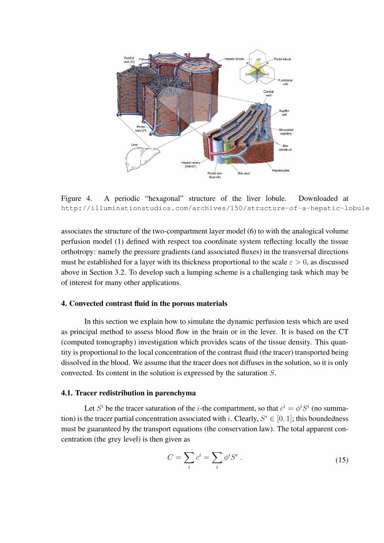
Figure 4. A periodic “hexagonal” structure of the liver lobule. Downloaded athttp://illuminationstudios.com/archives/150/structure-of-a-hepatic-lobule

associates the structure of the two-compartment layer model (6) to with the analogical volumeperfusion model (1) defined with respect toa coordinate system reflecting locally the tissueorthotropy: namely the pressure gradients (and associated fluxes) in the transversal directionsmust be established for a layer with its thickness proportional to the scale ε > 0, as discussedabove in Section 3.2. To develop such a lumping scheme is a challenging task which may beof interest for many other applications.

4. Convected contrast fluid in the porous materials

In this section we explain how to simulate the dynamic perfusion tests which are usedas principal method to assess blood flow in the brain or in the lever. It is based on the CT(computed tomography) investigation which provides scans of the tissue density. This quan-tity is proportional to the local concentration of the contrast fluid (the tracer) transported beingdissolved in the blood. We assume that the tracer does not diffuses in the solution, so it is onlyconvected. Its content in the solution is expressed by the saturation S.

4.1. Tracer redistribution in parenchyma

Let Si be the tracer saturation of the i-the compartment, so that ci = φiSi (no summa-tion) is the tracer partial concentration associated with i. Clearly, Si ∈ [0, 1]; this boundednessmust be guaranteed by the transport equations (the conservation law). The total apparent con-centration (the grey level) is then given as

C =∑

i

ci =∑

i

φiSi . (15)

The local conservation in a domain ω ⊂ Ω for the i-th compartment is expressed, as follows:∫ω

φi∂Si

∂t+

∫∂ω

wi · nSidΓ +∑

j

∫ω

Zij(S)J i

j =

∫ω

Sinfi+ +

∫ω

Sif i− , (16)

where Sin is the external source saturation, f i+ > 0 is the positive part (flow-in) of f i (f i

− isthe out-flow, vice versa) and the Z switches:

Zij(S) =

Si if J i

j > 0 ,Sj if J i

j ≤ 0 .(17)

From (16) we deduce the following problem: given wii and pii, for a given initial condi-tions Si(t = 0, x)i = Si

0(x)i given in Ω, find Si(t, x)i such that

φi∂Si

∂t+∇ · (Siwi) +

∑j

Zij(S)J i

j = Sinfi+ + Sif i

− x ∈ Ω, t > 0 , i = 1, . . . i ,

Sj given on ∂j−Ω(wj) ,

(18)

where ∂j−Ω(wj) = x ∈ ∂Ω| wj · n < 0Instead of the switch Z we may introduce corresponding index sets:

I i+ = j 6= i| J i

j > 0 , I i− = j 6= i| J i

j ≤ 0 . (19)

Further, by introducing the “true mean velocities” vi = (φi)−1wi, we can rewrite (18)1, asfollows:

φDviSi

Dt+ Si∇ · wi +

∑j∈Ii

−

SjJ ij +

∑j∈Ii

+

SiJ ij = Sinf

i+ + Sif i

− , (20)

where DviSi

Dtis the material derivative w.r.t. to vi.

4.2. Transport on branching network

We consider a branching network consisting of pipes and junctions. For such structurewe can derive the transport (advection) equations. Let ` =]x0, x1[, x0, x1 ∈ R be a pipe.Thus, by x we refer to the axial coordinate along the oriented(!) pipe with the end-pointsx0, x1, while by X ∈ R3 we mean the spatial positions associated with x. We consider avelocity w(x) and cross-section A(x) given at any x ∈ `, which satisfy the mass conservation(By Q we denote the flux in the pipe.)

∂x(wA) = ∂xQ = 0 , x ∈ `. (21)

Positivity of the convection velocity w is established in the context of the orientation of thepipe, i.e. T =

∫ x1

x01/w(x) dx is the transition time of the steady flow in the pipe.

It is now easy to derive the following equation for transport of the tracer, where S(x, t)

is the local instantaneous saturation; possible forms of the same equation are:

∂t(AS) + ∂x(wAS) = 0 ,

or

A(x)∂tS(x, t) +Q∂xS(x, t) = 0 ,

or

∂tS(x, t) + w(x)∂xS(x, t) = 0 , x ∈ `.

(22)

At the pipe ends we consider the boundary conditions:

S(x0, t) = S0(t) given for Q > 0 ,

S(x1, t) = S1(t) given for Q ≤ 0 .(23)

Transition times. We consider given saturations S0(t) and S1(t) at the end-points of pipe`e, see (23). Eq. (22)3 can be written using the material derivative as

Dw S(x, t)

D t= 0 , x ∈ `e , (24)

hence S(x1, t1) = S(x0, t0) where the transition time Te = t1 − t0 is Te =∫ x1

x0(w(x))−1dx.

Mixing and transport through junctions. We consider junctions (Xj, J j) connecting pipes`kk∈Jj , where Xj ∈ R3 is the j-th junction spatial position and J j is the set of indices ofpipes connected at the junction. At any junction, a unique saturation Sj is computed using anobvious conservation law. The mean junction saturation Sj satisfies∑

e∈Jj+

SeAevje + Sj

∑e∈Jj

−

Aevje = 0 ,

where

vje = +we if e ends at junction j ,vj

e = −we if e begins at junction j ,J j

+ = e ∈ J j| ve ≥ 0 ,J j− = e ∈ J j| ve < 0 ,

(25)

so that velocities we in pipes `e define ve depending on the oriented network topology. Wecan call J j

+ the index set of sources and J j− the index set of sinks.

Assembling equations of the transport on the network Due to (24) and knowledge of thetransition times, the state of the transport is described by the junction saturations Sj(t)j .Equations of the model are assembled, as follows:

1. For `e with a given we define the source junction i = i(e), such that e ∈ J−, i.e. vie < 0.

It means, that S(x, t) for x ∈ `e is driven by Si(t).

2. The sink junction j of the pipe e, where e ∈ J+, is associated with the general formequation (25), where Se(t) := Si(t− Te), where i = i(e).

3. Let a junction j is coupled directly with junctions k+e e with e ∈ J j (we consider two

junctions (k+e , k

−e ), i.e. “source-sink” couple, for each junction. The junction equation

at time t is

Sj(t)∑e∈Jj

−

Aevje +

∑e∈Jj

+

AevjeS

ke(t− Te) = 0 . (26)

The junction equations (26) can be evaluated for discretized time interval, i.e. fort ∈ tnn where tn = t0 +n∆t. Obviously, for a given Te, the saturation at tn−Te ∈ [tp, tp+1]

is approximated using the average of values at tp and tp+1 .

5. Numerical examples

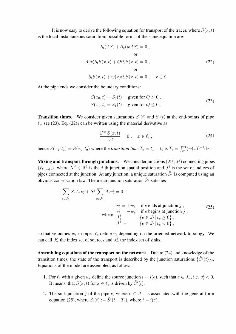
Preliminary testing of the above described multiscale modeling approach was per-formed for a simplified model of pig liver, Fig. 5 (left); domain Ω is the cube into whichtwo perfusion trees handled by the “1D” model penetrate; they are described schematically inFig. 5(right), whereby the lengths and average diameters of the main hepatic veins and theirsegments listed in Table 1 are based on a sonography examination of an experimental pigdone at the Faculty of Medicine in Pilsen, Charles University in Prague. Effects of the hepaticartery were not considered in the present example.

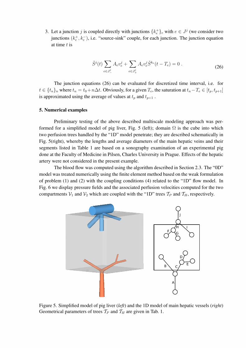
The blood flow was computed using the algorithm described in Section 2.3. The “0D”model was treated numerically using the finite element method based on the weak formulationof problem (1) and (2) with the coupling conditions (4) related to the “1D” flow model. InFig. 6 we display pressure fields and the associated perfusion velocities computed for the twocompartments V1 and V2 which are coupled with the “1D” trees TP and TH , respectively.

Figure 5. Simplified model of pig liver (left) and the 1D model of main hepatic vessels (right)Geometrical parameters of trees TP and TH are given in Tab. 1.

Flow in V1 Flow in V2

Figure 6. Perfusion velocities in parallel sectors V1 (top left) and V2 (top right) connectedwith the “1D” trees TP and TH , respectively, see Fig. 5. The associated pressure differencesindicate blood filtration in the capillary system, i.e flux between the two sectors.

0 0.5 1 1.5 2 2.50

0.2

0.4

0.6

0.8

time

Sin

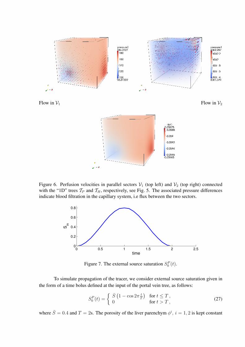
Figure 7. The external source saturation SP0 (t).

To simulate propagation of the tracer, we consider external source saturation given inthe form of a time bolus defined at the input of the portal vein tree, as follows:

SP0 (t) =

S(1− cos 2π t

T

)for t ≤ T ,

0 for t > T ,(27)

where S = 0.4 and T = 2s. The porosity of the liver parenchym φi, i = 1, 2 is kept constant

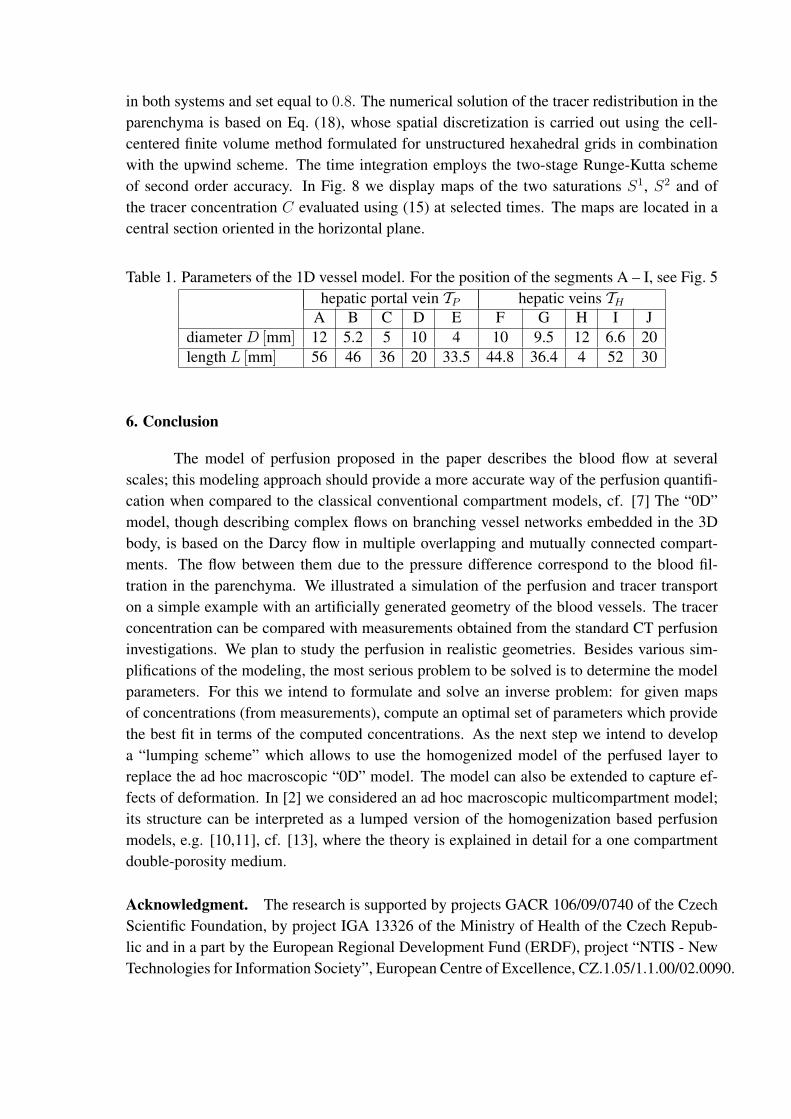
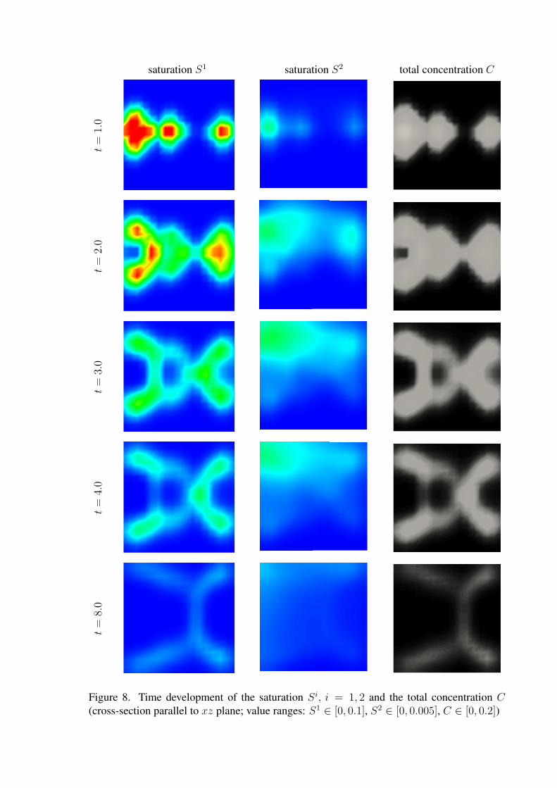
in both systems and set equal to 0.8. The numerical solution of the tracer redistribution in theparenchyma is based on Eq. (18), whose spatial discretization is carried out using the cell-centered finite volume method formulated for unstructured hexahedral grids in combinationwith the upwind scheme. The time integration employs the two-stage Runge-Kutta schemeof second order accuracy. In Fig. 8 we display maps of the two saturations S1, S2 and ofthe tracer concentration C evaluated using (15) at selected times. The maps are located in acentral section oriented in the horizontal plane.

Table 1. Parameters of the 1D vessel model. For the position of the segments A – I, see Fig. 5hepatic portal vein TP hepatic veins TH

A B C D E F G H I Jdiameter D [mm] 12 5.2 5 10 4 10 9.5 12 6.6 20length L [mm] 56 46 36 20 33.5 44.8 36.4 4 52 30

6. Conclusion

The model of perfusion proposed in the paper describes the blood flow at severalscales; this modeling approach should provide a more accurate way of the perfusion quantifi-cation when compared to the classical conventional compartment models, cf. [7] The “0D”model, though describing complex flows on branching vessel networks embedded in the 3Dbody, is based on the Darcy flow in multiple overlapping and mutually connected compart-ments. The flow between them due to the pressure difference correspond to the blood fil-tration in the parenchyma. We illustrated a simulation of the perfusion and tracer transporton a simple example with an artificially generated geometry of the blood vessels. The tracerconcentration can be compared with measurements obtained from the standard CT perfusioninvestigations. We plan to study the perfusion in realistic geometries. Besides various sim-plifications of the modeling, the most serious problem to be solved is to determine the modelparameters. For this we intend to formulate and solve an inverse problem: for given mapsof concentrations (from measurements), compute an optimal set of parameters which providethe best fit in terms of the computed concentrations. As the next step we intend to developa “lumping scheme” which allows to use the homogenized model of the perfused layer toreplace the ad hoc macroscopic “0D” model. The model can also be extended to capture ef-fects of deformation. In [2] we considered an ad hoc macroscopic multicompartment model;its structure can be interpreted as a lumped version of the homogenization based perfusionmodels, e.g. [10,11], cf. [13], where the theory is explained in detail for a one compartmentdouble-porosity medium.

Acknowledgment. The research is supported by projects GACR 106/09/0740 of the CzechScientific Foundation, by project IGA 13326 of the Ministry of Health of the Czech Repub-lic and in a part by the European Regional Development Fund (ERDF), project “NTIS - NewTechnologies for Information Society”, European Centre of Excellence, CZ.1.05/1.1.00/02.0090.

saturation S1 saturation S2 total concentration C

t=

1.0

t=

2.0

t=

3.0

t=

4.0

t=

8.0

Figure 8. Time development of the saturation Si, i = 1, 2 and the total concentration C(cross-section parallel to xz plane; value ranges: S1 ∈ [0, 0.1], S2 ∈ [0, 0.005], C ∈ [0, 0.2])

7. REFERENCES

[1] R. Cimrman and et al. Software, finite element code and applications. SfePy home page.,2011. http://sfepy.org.

[2] R. Cimrman and E. Rohan. On modelling the parallel diffusion flow in deforming porousmedia. Math. and Computers in Simulation, 76:34–43, 2007.

[3] D. Cioranescu, A. Damlamian, and G. Griso. The periodic unfolding method in homog-enization. SIAM Journal on Mathematical Analysis, 40(4):1585–1620, 2008.

[4] C. D’Angelo. Multiscale 1D-3D models for tissue perfusion and applications. In Proc.of the 8th.World Congress on Computational Mechanics (WCCM8), 2008. Venice, Italy.

[5] L. Formaggia, A. Quarteroni, and A. Veneziani. Cardiovascular Mathematics: Modelingand Simulation of the Circulatory System. Springer, 2009.

[6] T.S. Koh, C.K.M. Tan, L.H.D. Cheong, and C.C.T. Lim. Cerebral perfusion map-ping using a robust and efficient method for deconvolution analysis of dynamic contrast-enhanced images. NeuroImage, 32:643–653, 2006.

[7] R. Materne, B. E. Van Beers, A. M. Smith, I. Leconte, J. Jamart, J.-P. Dehoux, A. Keyeux,and Y. Horsmans. Non-invasive quantification of liver perfusion with dynamic computedtomography and a dual-input one-compartmental model. Clinical Science, 99:517–525,2000.

[8] E. Rohan. Homogenization approach to the multi-compartment model of perfusion. Proc.Appl. Math. Mech., 6:79–82, 2006.

[9] E. Rohan. Homogenization of the perfusion problem in a layered double-porous mediumwith hierarchical structure. 2010. Submitted.

[10] E. Rohan and R. Cimrman. Two-scale modelling of tissue perfusion problem usinghomogenization of dual prous media. Int. Jour. for Multiscale Comput. Engrg., 8:81–102, 2010.

[11] E. Rohan and R. Cimrman. Multiscale FE simulation of diffusion-deformation processesin homogenized dual-porous media. Math. Comp. Simul., 2011. In Press.

[12] E. Rohan and V. Lukes. Modeling tissue perfusion using a homogenized model withlayer-wise decomposition. In F. Breitenecker I. Troch, editor, Proc. of the MATHMOD2012 Conf. TU Vienna, 2012.

[13] E. Rohan, S. Naili, R. Cimrman, and T. Lemaire. Multiscale modeling of a fluid saturatedmedium with double porosity: Relevance to the compact bone. Jour. Mech. Phys. Solids,60:857—881, 2012.

[14] R.E. Showalter and D.B. Visarraga. Double-diffusion models from a highly heteroge-neous medium. Journal of Mathematical Analysis and Applications, 295:191–210, 2004.