Towards Automating Precision Irrigation: Deep Learning to Infer LocalSoil Moisture Conditions from Synthetic Aerial Agricultural Images

David Tseng∗,1 David Wang∗,1 Carolyn Chen,1 Lauren Miller,1 William Song,1

Joshua Viers,2 Stavros Vougioukas,3 Stefano Carpin,4 Juan Aparicio Ojea,5 Ken Goldberg1,6

Abstract— Recent advances in unmanned aerial vehiclessuggest that collecting aerial agricultural images can be cost-efficient, which can subsequently support automated precisionirrigation. To study the potential for machine learning to learnlocal soil moisture conditions directly from such images, wedeveloped a very fast, linear discrete-time simulation of plantgrowth based on the Richards equation. We use the simulatorto generate large datasets of synthetic aerial images of avineyard with known moisture conditions and then compareseven methods for inferring moisture conditions from images,in which the "uncorrelated plant" methods look at individualplants and the "correlated field" methods look at the entirevineyard: 1) constant prediction baseline, 2) linear SupportVector Machines (SVM), 3) Random Forests UncorrelatedPlant (RFUP), 4) Random Forests Correlated Field (RFCF),5) two-layer Neural Networks (NN), 6) Deep ConvolutionalNeural Networks Uncorrelated Plant (CNNUP), and 7) DeepConvolutional Neural Networks Correlated Field (CNNCF).Experiments on held-out test images show that a globally-connected CNN performs best with normalized mean absoluteerror of 3.4%. Sensitivity experiments suggest that learnedglobal CNNs are robust to injected noise in both the simulatorand generated images as well as in the size of the trainingsets. In simulation, we compare the agricultural standard offlood irrigation to a proportional precision irrigation controllerusing the output of the global CNN and find that the lat-ter can reduce water consumption by up to 52% and isalso robust to errors in irrigation level, location, and timing.The first-order plant simulator and datasets are available athttps://github.com/BerkeleyAutomation/RAPID.

I. INTRODUCTION

An estimated 75% of freshwater is used in agriculture,but only between 5% and 30% of this irrigation is absorbedby plants [34]. Environmental scientists predict that waterscarcity will be a major issue in the coming decades [35].

In precision agriculture, measurements determine the statusof individual plants to modify irrigation and other farmresources accordingly [24]. Recent advances in robotics canfacilitate precision irrigation with devices that interact withthe plants and irrigation pipelines directly [7, 11] or monitorconditions such as soil moisture [27]. Others take advantageof recent advances in unmanned aerial vehicles (UAVs) [10,

The AUTOLab at UC Berkeley (automation.berkeley.edu).1EECS, UC Berkeley, {davidtseng, dmwang,carolyn.chen, william.song, goldberg}@berkeley.edu,lauren.mohr.miller@gmail.com; 2Center for Watershed Sciences,UC Merced, jviers@ucmerced.edu; 3Biological and AgriculturalEngineering, UC Davis, svougioukas@ucdavis.edu; 4Schoolof Engineering, UC Merced, scarpin@ucmerced.edu; 5SiemensCorporation, Corporate Technology, juan.aparicio@siemens.com;6IEOR, UC Berkeley.* These authors contributed equally to the paper.

Fig. 1: Top left: Moisture dissipation pattern. Top right: Syntheticaerial image generated by the simulator. We use the simulator togenerate 1,200 examples to form a training dataset, and we usesupport vector machines, random forests, and convolutional neuralnetworks to infer moisture dissipation patterns from images. Bottomleft: Example of a test image. Bottom right: Moisture dissipationpredicted by the CNN.

37]. Under the NSF National Robotics Initiative (NRI), theRobot Assisted Precision Irrigation Delivery (RAPID) projectinvestigates how co-robotic devices can be used to adjustirrigation emitters. Prior work in this project has involveddeveloping robotic tools to adjust emitters [4, 5, 11] androuting algorithms for mobile robots [31, 32].

In precision irrigation, soil moisture conditions determinethe amount of irrigation needed. To the best of our knowledge,there are no publicly available datasets with pairs of aerialimages and local soil moisture conditions at the plant level.In this paper, we explore machine learning methods tolearn mappings between images and soil moisture dissipationpatterns and how the learned models could control precisionirrigation at the plant level. An overview is shown in Fig.1. We study this problem in simulation as a first stepto explore the potential of machine learning for precisionirrigation before undertaking extremely costly physical fieldexperiments. We present a first-order simulator that modelsthe local soil moisture at each plant over time using a discrete-time, linear approximation of the Richards equation [33] forsoil water flow. One major benefit of this first-order simulatoris its speed, which allows us to quickly generate datasets ofvineyard images based on different soil moisture dissipationpatterns. We perform experiments with seven methods to learn

the inverse mapping from images to soil moisture dissipationpatterns, in which the "uncorrelated plant" methods lookat individual plants and the "correlated field" methods lookat the entire vineyard: 1) constant prediction baseline, 2)linear Support Vector Machines (SVM), 3) Random ForestsUncorrelated Plant (RFUP), 4) Random Forests CorrelatedField (RFCF), 5) two-layer Neural Networks (NN), 6) DeepConvolutional Neural Networks Uncorrelated Plant (CNNUP),and 7) Deep Convolutional Neural Networks Correlated Field(CNNCF). We analyze the robustness of these models byconducting sensitivity experiments, exposing the learningmethods to limited numbers of training examples and injectingtwo types of noise: simulation noise, where we perturb thesimulator dynamics, and image noise, where we perturb thegenerated aerial images. We also implement a proportionalprecision irrigation controller in simulation using the learnedmodels.

This paper makes the following contributions:1) A novel first-order agricultural simulator that uses a

discrete-time, linear approximation of the Richardsequation for soil moisture dissipation.

2) A labeled dataset for supervised learning, in which theexamples are pairs of soil moisture dissipation patternsand the generated synthetic aerial images, containing1200 training examples and 200 test examples.

3) Experiments comparing seven machine learning meth-ods that are able to learn inverse models from aerial im-ages to the underlying soil moisture dissipation patternsand experiments with a proportional precision irrigationcontroller using the learned globally-connected CNN.

II. RELATED WORK

A. Agricultural Simulators

Several crop simulators have been published in the agricul-tural community. WOFOST [8], DSSAT [19], and MONICA[26] simulate aggregate crop statistics such as yield based onparameters such as weather and location. Other simulatorsprovide similar information for specific crops, like SUNFLO[6] for sunflowers and MaizSim [38] for corn. Such simulatorsprovide accurate estimates by modeling plant biology and theenvironment but generally output aggregate crop statistics overentire vineyards rather than on a per-plant basis, which cannotbe used to generate labeled data for a precision irrigationmodel. While our first-order simulator does not explicitlymodel physical processes at the level of plant biology, suchas in [22], it provides reasonable simulated aerial images ofa field of crops, given local soil moisture dissipation ratesat each of the plants. A comparison between the simulatoroutput and a real vineyard is shown in Fig. 2.

B. Agricultural Image Datasets

To the best of our knowledge, large-scale, public datasetsof paired aerial field images and corresponding local soilconditions for individual plants do not exist. Of the existingagricultural image datasets, many are tailored to classificationand segmentation experiments. Söderkvist published a datasetof leaves from Swedish trees [29], Wu et al. published the

Fig. 2: Example of (left) a true aerial image of a vineyard ofSymphony grapes in Cowell Ranch of Snelling, CA and (right) asynthetic aerial image generated by the first-order simulator. Thereis inherent heterogeneity of plant growth in both.Flavia dataset of leaves from 33 plant species [36], andKumar et al. published a combined dataset of high-resolutionleaves from the Smithsonian collection and images takenfrom mobile phones in the field [21]. These labeled datasetsare used for plant species identification. Recently, Haug etal. [16] published a labeled dataset of aerial field imagesfor the purpose of segmentation and crop/weed classification.Hassan-Esfahani et al. took aerial images of fields using aUAV [13–15] as part of the AggieAir™ project led by CalCoopmans and Alfonso Torres Rua. They also made local soilmoisture measurements to create a dataset with 184 points,demonstrating the potential to collect a larger dataset. In thispaper, we generate a dataset that consists of 1,400 syntheticaerial images of a vineyard and corresponding local soilmoisture conditions at each plant.

C. Machine Learning in Agriculture

There exist previous applications of machine learning inagricultural settings to learn soil moisture conditions. Schmitzet al. [28] used neural networks to learn the relationshipbetween irrigation and soil moisture profiles for drip irrigationto optimize soil moisture. Möller et al. [25] utilized visual andthermal images of crops from a Forward-Looking InfraredRadar (FLIR) thermal imaging system to estimate crop waterstress index (CWSI) [18]. Hassan-Esfahani et al. estimatedtopsoil moisture profiles using Relevance Vector Machines,Multilayer Perceptrons, and Bayesian Neural Networks andmultiple types of images collected using a UAV [13–15] inthe AggieAir™ project. Other applications involve SVMs orRVMs to estimate soil parameters using a variety of datasuch as weather data and crop physiological characteristicsinstead of aerial images [2, 3, 39]. In this paper, we present anend-to-end simulation system that generates synthetic aerialimages and learns mappings from the images to local soilmoisture conditions using both previously used techniquesas well as deep CNN’s. We also evaluate the effectivenessof precision irrigation controllers using the learned models,which can be more efficient than traditional methods such asflood irrigation. For example, Mateos et al. [23] compareddrip irrigation and furrow irrigation, a type of flood irrigation,in cotton crops and used up to 46% less water with the formerstrategy.

III. PROBLEM STATEMENT AND ASSUMPTIONS

Our goal is to learn a model that takes a synthetic RGBaerial image as input and outputs predictions of soil moisture

dissipation patterns. We first address the forward problem:given soil moisture dissipation patterns, rapidly generate asynthetic 320×320 RGB image of a vineyard containing pplants at t days after the plants are planted, given d ∈ Rp,the local soil moisture dissipation rate at each of the plants.

Here, we present modeling assumptions for the designof the simulator and for the prediction of soil moisturedissipation patterns. For the growth of each plant in thevineyard, we use the model of one-dimensional vertical waterflow to simulate the dynamics of water flow in soil. This canbe expressed with the following nonlinear partial differentialequation, which is the basis of the well-known Richardsequation [33]:

∂ s∂ t

=−∂q∂ z−S(h),

where s is the volumetric water content in the soil (cm3 ofwater per cm3 of soil), t is the time (days), ∂q

∂ z is a term thatdescribes the flow of soil water as a result of differences insoil water potential, and S(h) is a term that describes the soilwater extraction by plant roots (cm3 of water per cm3 of soilper day). In this paper, we refer to s as a measure of soilmoisture. In the simulator, we approximate this differentialequation using the following discrete linear update equation,which is why we refer to the simulator as being first-order:

st = st−1 +∆st , where ∆st =−(r−at)−U(t).

Here, r is the soil drainage rate, at is the irrigation rateapplied during day t, and U(t) is the rate at which plantwater uptake occurs during day t. In relation to the Richardsequation, we approximate − ∂q

∂ z with at − r, the rate at whichwater becomes available for use during day t, and we alsohave S(h) = U(t). Under optimal moisture conditions, thefollowing equation for U(t) holds [9]:

U(t) = R(t) ·Tp(t),

where R(t) is a factor related to root length density at time t,and Tp(t) is potential transpiration rate (cm per day) that isdriven by weather. In the first-order simulator, we assume thefollowing remain constant over time for a particular plant: R(t)(water uptake capacity due to root size does not change asthe plant grows), Tp(t) (weather does not change significantlyto cause variation in daily plant water transpiration), andr (the local soil drainage rate does not vary). Thus, in thesimulator, U(t) is also constant over time, and we simplywrite U . Under these assumptions, our discrete-time linearupdate equation can be written as follows:

st = st−1 +at − (r+U) = st−1 +at −d.

We define d = r+U to be the moisture dissipation rate, whichis a measure of local water loss, e.g., due to soil drainage,uptake by the plant, evaporation, etc. We attempt to learn dfrom the images. We also assume linear plant growth, whereeach plant grows a constant f new leaves on day t if st > 0.The simulator is described in further detail in Section IV-A.

The first objective is to use the simulator to generate adataset containing pairs of ground-truth local soil moisture

dissipation rates of the plants d and the resulting image x. Wedefine d(i) and x(i) to be the soil moisture dissipation ratesand corresponding image, respectively, for the i-th examplein the training dataset for i = 1 to Ntrain. Using the sameprocess, we generate a test dataset containing Ntest examples.

The next objective is to learn the inverse model Hθ∗ fromthe images {x(i)}Ntrain

i=1 to the local soil moisture dissipationrates {d(i)}Ntrain

i=1 of the plants in the images, where Hrepresents the model, θ represents the parameters of H, andHθ (x) represents the predicted soil moisture dissipation ratesgiven by model Hθ on input image x. Ultimately, we seekto find θ ∗ ∈Θ, where Θ represents the space of parametersθ , such that the expected loss L over all possible simulatedimages that can result from the process described in SectionIV-B is minimized, i.e.,

θ∗ = argmin

θ∈Θ

E[L(d,Hθ (x))].

We want to minimize the mean squared error loss function:

L(d,Hθ (x)) =1p

p∑j=1

(d j−Hθ (x) j))2 .

Since it is difficult to minimize the expected loss, we seek θ ∗

that minimizes the loss over our generated training dataset,

θ∗ = argmin

θ∈Θ

Ntrain∑i=1

L(d(i),Hθ (x(i))).

IV. FIRST-ORDER PLANT SIMULATOR

A. Discrete Time Simulator

We define a vineyard of length l and width w. We assumen columns of plants uniformly spaced across the vineyardand m individual plants uniformly spaced within each columnfor a total of mn individual plants.

The simulator generates aerial images of the vineyard atdiscrete timesteps (days), based on the following parametersand inputs.• d ∈ Rmn is a vector of local soil moisture dissipation

rates for each of the plants, measuring the rate of waterloss due to a combination of soil drainage and uptakeby the plant itself. These rates do not vary over time.

• a(t) ∈Rmn is a vector of applied irrigation rates for eachplant on day t for t = 1,2, . . . .

In this model, the primary factor for determining plantgrowth is soil moisture. Letting s(t) ∈ Rmn denote a vectorof local soil moistures for each of the plants during day t,these vectors are initialized and updated as follows, alwaysensuring that the soil moisture is non-negative:

s(0) = 1 (IV.1)

s(t) = max(s(t−1)+a(t)−d,0) for t = 1,2, . . . (IV.2)

In each timestep, the visible growth of the plant dependson the current soil moisture value. If the soil moisture ispositive, a fixed number of leaves f is added to each plant.The location of the new leaves are sampled from a multivariate

Fig. 3: (left) We show the soil moisture dissipation rate map of thevineyard generated using the process described in Section IV-B. Redindicates higher dissipation rates, and blue indicates lower rates. Aconstant irrigation rate is applied at each time step, and we showthe aerial image generated by the simulator in subsequent imagesat timesteps 5, 10, and 15, respectively. Note that only the imagesfrom the 10th timestep are used in the training and test datasets.

normal distribution with a mean at the center of the plant anda covariance matrix proportional to the current soil moisture.If the soil moisture is 0, then the plant is considered under-watered, no leaves are added, and the existing leaves arecolored by a shade of yellow.

For experiments, we use the following simulator parametervalues: l = 100 and w = 100 for the vineyard dimensions,m = 20 and n = 10 for the number of plants, and f = 7 forthe number of leaves added per plant in each timestep. Fig.3 shows an example of the simulation output.

B. Dataset Generation

To generate the dataset, we apply a constant irrigation rateof 0.5 to every plant at each timestep, and we generate anindependent soil moisture dissipation map for each example.To simulate variability in soil moisture dissipation rates dueto variations in soil, elevation, sun, and wind, we generatedissipation rates for each example in the dataset accordingto the following process:

1) Choose the number of areas k of high dissipation rateuniformly at random between 2, 3, and 4.

2) We model each of the areas of high dissipation rate asa multivariate normal distribution. In the vineyard oflength l and width w, we choose the center µ(i) ∈ R2

for each of the k areas of high dissipation rate uniformlyat random.

3) We randomize a diagonal covariance matrix, Σ(i), foreach distribution. We assume independence betweenthe two directions and select standard deviations inboth directions uniformly at random in ranges definedby minσx , maxσx , minσy , and maxσy ,

4) After defining these areas of high dissipation rate, wetake a linear combination of the distributions to obtaina density de(x,y) of effective dissipation rate over theentire vineyard, i.e.

de(x,y) =k∑

i=1

c · exp

− (x−µ(i)1 )2

2Σ(i)1,1

2−

(y−µ(i)2 )2

2Σ(i)2,2

2

.

We use c = 0.4 as a scaling factor so that eachmultivariate normal distribution attains a maximumvalue of c. We normalize so that the local soil moisturedissipation rate of a plant at location (x,y) in thevineyard is d(x,y) = min(de(x,y),1).

For each example in the dataset, we use the process outlinedabove to generate the soil moisture dissipation map, and we

run the simulator to obtain the corresponding aerial image. Forthe ranges of standard deviations in the multivariate normaldistributions, we use minσx = 10, maxσx = 40, minσy = 10,and maxσy = 40. Based on visual inspection, we decided touse the generated aerial image at timestep 10 because, at thispoint, the image appears most representative of true imagesof vineyards. We generated 1,200 independent examples forthe training set and 200 independent examples for the test set,which took 3 seconds per example on a machine with an Inteli7 Core Processor and 16 GB of RAM. The leftmost imagein Fig. 3 shows an example generated from this process.

V. LEARNING THE INVERSE MODEL

We consider seven methods of learning the inverse modelHθ : 1) constant prediction baseline, 2) linear Support VectorMachines (SVM), 3) Random Forests Uncorrelated Plant(RFUP), 4) Random Forests Correlated Field (RFCF), 5)two-layer Neural Networks (NN), 6) Deep ConvolutionalNeural Networks Uncorrelated Plant (CNNUP), and 7) DeepConvolutional Neural Networks Correlated Field (CNNCF).Each method produces a candidate inverse model thattakes in a simulated aerial image as input and outputs thecorresponding estimated moisture dissipation rates, and eachcandidate inverse model has its own separate set of parameters.In addition, for each method, we use the same training setto tune the model’s parameters and the same testing set toevaluate the metrics described in Section VI-A. We alsorandomly split the initial training dataset into a training setwith 1,000 examples and a validation set with 200 examplesin our methods to tune hyperparameters.

We evaluated two variants of some of our methods,comparing learning dissipation rates for the entire vineyardsimultaneously vs. learning rates for individual plants. Forthe "uncorrelated" methods, which look at the vineyard ona plant-by-plant basis and predict moisture dissipation ratesfor each plant independently from neighboring plants, thesimulated images were preprocessed by cropping individualplants from the original vineyard images. On the other hand,the "correlated" methods look at the entire image of thevineyard and output a vector of 200 dissipation rates.

A. Constant Prediction Baseline

As a baseline for comparison, this method produces amodel that outputs a constant prediction c, the mean of allof the moisture dissipation rates in the training set.

B. Linear Support Vector Machine Regression (SVM)

We trained 200 linear support vector machine (SVM)regressors using the RGB values of the images as features,where each SVM learns the moisture dissipation rate at aparticular plant location. This was implemented using scikit-learn. Since the number of features is significantly greaterthan the number of training examples, the dimensionality isalready high, and using more complex kernels would imposeadditional computation time. Thus, we use a linear kernelinstead of a radial basis function (RBF) kernel [17].

Fig. 4: The CNN architectures for the methods described in Sec. V-F and V-G. (a) The CNN Uncorrelated Plant Method. Each individualplant image is cropped from the original simulated vineyard image and is input to the above CNN. (b) The CNN Correlated Field Method.The simulated vineyard image is input to the above CNN, and the moisture dissipation rates for all 200 plants are estimated together.

C. Random Forest Uncorrelated Plant Method (RFUP)

In this method, we look at images of individual plants witha random forest, using the image RGB values as features.The simulated images are preprocessed using the croppingmethod mentioned in the beginning of Section V before beinggiven to a RF as input. The RF was implemented with 10decision trees using scikit-learn with a maximum depth of20, and parameters were determined using the validation set.

D. Random Forest Correlated Field Method (RFCF)

This method is similar to that of Section V-C, exceptthe RF trains on images of the entire vineyard. The RFimplementation is the same as the one described in SectionV-C.

E. Two-Layer Neural Network (NN)

We implemented a two-layer feed-forward NN to serve ascomparison with the convolutional NN architectures describedin Sections V-F and V-G. It is also similar to the architectureused by [14] in the AggieAir™ project, but not directlycomparable. In this method, aerial images are preprocessedusing the cropping process described earlier. The RGB valuesof the cropped plant images are provided as input into theNN, which consists of a hidden layer with 4096 units, ReLUactivations [12], and an output layer with a single nodecontaining the moisture dissipation prediction. The estimateddissipation rates for individual plant images are concatenatedtogether to form an output with 200 predictions. In thisTensorFlow [1] implementation, we perform training withdropout [30] of probability 0.25 for regularization, Kingma etal.’s Adam [20] optimization with an initial learning rate of1×10−3, and 40 epochs of learning. We use the validationset to tune hyperparameters.

F. CNN Uncorrelated Plant Method (CNNUP)

In this method, the images are cropped and provided asinput to a CNN, similar to Section V-E. The CNN architectureused in this method is illustrated in Fig. 4a. The CNNwas implemented using TensorFlow [1], the initial learningrate for the Adam algorithm was set to 1× 10−3, and weused mini-batches of 25 images, which were values that weobserved lead to relatively quick convergence. We optimizedthe parameters θ in the CNN by applying Adam algorithmand used ReLU activation, dropout of probability 0.25, andtraining for 40 epochs. We use our CNN’s performance onthe validation set to tune hyperparameters.

G. CNN Correlated Field Method (CNNCF)

This method is similar to the CNN Uncorrelated PlantMethod in Sec. V-F, except that the whole image is used asinput. The architecture used for this method is described inFig 4b. Compared to the architecture used in V-F, CNNCFuses an additional convolutional layer and max pool layer,since the input is larger. The implementation and optimizationare the same, but we use an initial learning rate 1×10−4 andtrain for 30 epochs.

Method Q1 Mean M Q3 TrainingTime (s)

Const. Prediction 0.082 0.177 0.162 0.246 N/ASVM 0.015 0.038 0.030 0.053 4141RFUP 0.030 0.071 0.060 0.101 578RFCF 0.047 0.109 0.094 0.152 655

Two-Layer NN 0.037 0.086 0.075 0.119 243CNNUP 0.021 0.054 0.044 0.077 538CNNCF 0.012 0.034 0.027 0.047 603

TABLE I: Results from applying each method to the test dataset.We report the following statistics over all absolute value predictionerrors in the test dataset: 25th percentile (Q1), mean, median (M),and 75th percentile (Q3). We also report the training time (s) foreach of the methods on a machine with an Intel Core i7-6850kProcessor and three Nvidia Titan X Pascal GPU’s.

VI. EXPERIMENTS

A. Evaluation Metrics

We use the median absolute error as our main evaluationmetric because of its interpretability as the normalizedprediction error. We define the absolute error for a singlemoisture dissipation rate as |d j−H(x) j|, where H(x) j is theestimated moisture dissipation rate of plant j in input imagex, and d j is the actual dissipation rate of plant j. We reportthe median, since our distributions of absolute value errorstend to be skewed; in the simulator, plants with higher soilmoisture dissipation rates have less variability in appearancethan plants with lower dissipation rates. As a result, all modelstend to have higher absolute error when predicting higherdissipation rates. We report the interquartile range of theabsolute errors of all moisture dissipation rates in the test setto show the distribution.

B. Estimating Moisture Dissipation Rates in the Test Dataset

We evaluated the performance of each method on the testdataset. Each method was trained on the same training andvalidation set, with no added noise. Table I lists the resultingmedian and mean, as well as the first and third quartiles, ofthe absolute errors in the test dataset. We found that CNNCF

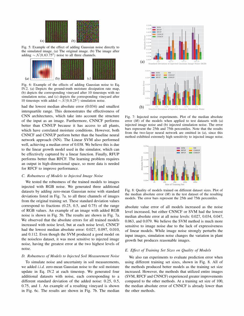
Fig. 5: Example of the effect of adding Gaussian noise directly tothe simulated image. (a) The original image. (b) The image afteradding ∼N (0,63.752) noise to all three channels.

Fig. 6: Example of the effects of adding Gaussian noise to Eq.IV.2. (a) Depicts the ground-truth moisture dissipation rate map,(b) depicts the corresponding vineyard after 10 timesteps with nosimulation noise, and (c) depicts the corresponding vineyard after10 timesteps with added ∼N (0,0.252) simulation noise.

had the lowest median absolute error (0.034) and smallestinterquartile range. This demonstrates the effectiveness ofCNN architectures, which take into account the structureof the input as an image. Furthermore, CNNCF performsbetter than CNNUP because it has access to all plants,which have correlated moisture conditions. However, bothCNNCF and CNNUP perform better than the baseline neuralnetwork approach (NN). The Linear SVM also performedwell, achieving a median error of 0.038. We believe this is dueto the linear growth model used in the simulator, which canbe effectively captured by a linear function. Finally, RFUPperforms better than RFCF. The learning problem requiresan output in high-dimensional space, so more data is neededfor RFCF to improve performance.

C. Robustness of Models to Injected Image Noise

We tested the robustness of the trained models to imagesinjected with RGB noise. We generated three additionaldatasets by adding zero-mean Gaussian noise with standarddeviations listed in Fig. 7a. to all three channels of imagesfrom the original training set. These standard deviation valuescorrespond to fractions (0.25, 0.5, and 0.75) of the rangeof RGB values. An example of an image with added RGBnoise is shown in Fig. 5b. The results are shown in Fig. 7a.We observed that the absolute errors for all trained modelsincreased with noise level, but at each noise level, CNNCFhad the lowest median absolute error: 0.027, 0.097, 0.010,and 0.112. Even though the SVM produced a good model onthe noiseless dataset, it was most sensitive to injected imagenoise, having the greatest error at the two highest levels ofnoise.

D. Robustness of Models to Injected Soil Measurement Noise

To simulate noise and uncertainty in soil measurements,we added i.i.d. zero-mean Gaussian noise to the soil moistureupdate in Eq. IV.2 at each timestep. We generated fouradditional datasets with noise, each corresponding to adifferent standard deviation of the added noise: 0.25, 0.5,0.75, and 1. An example of a resulting vineyard is shownin Fig. 6c. The results are shown in Fig. 7b. The median

(a)

(b)

Fig. 7: Injected noise experiments. Plot of the median absoluteerror (M) of the models when applied to test datasets with (a)injected image noise and (b) injected simulation noise. The errorbars represent the 25th and 75th percentiles. Note that the resultsfrom the two-layer neural network are omitted in (a), since thismethod exhibited extremely high sensitivity to injected image noise.

25 100 400 1000 2000Size of Training Set

0.00

0.05

0.10

0.15

0.20

0.25

Absolute Error

SVMRFUPRFCF

NNCNNUPCNNCF

Fig. 8: Quality of models trained on different dataset sizes. Plot ofthe median absolute error (M) in the test dataset of the resultingmodels. The error bars represent the 25th and 75th percentiles.

absolute value error of all models increased as the noiselevel increased, but either CNNCF or SVM had the lowestmedian absolute error at all noise levels: 0.027, 0.034, 0.047,0.063, and 0.079. We believe the SVM method is much moresensitive to image noise due to the lack of expressivenessof linear models. While image noise strongly perturbs theinput images, simulation noise changes the variation in plantgrowth but produces reasonable images.

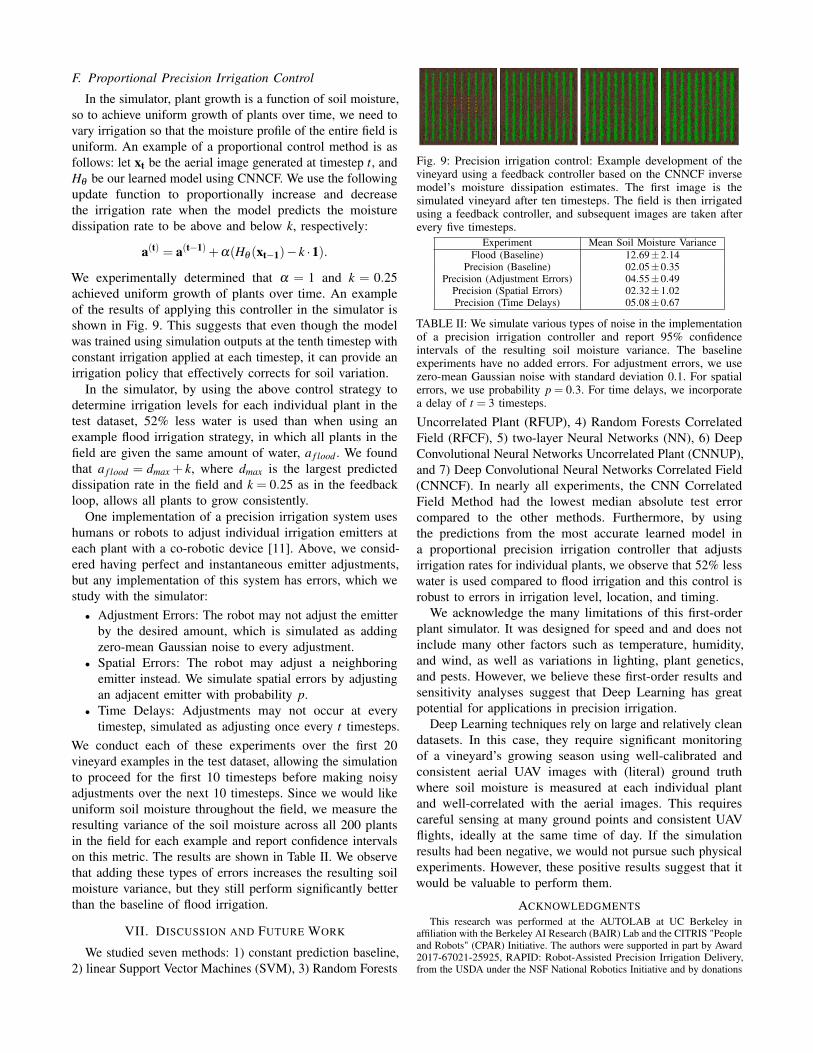
E. Effect of Training Set Sizes on Quality of Models

We also ran experiments to evaluate prediction error whenusing different training set sizes, shown in Fig. 8. All ofthe methods produced better models as the training set sizeincreased. However, the methods that utilized entire images(SVM, RFCF and CNNCF) experienced greater improvementscompared to the other methods. At a training set size of 100,the median absolute error of CNNCF is already lower thanthe other methods.

F. Proportional Precision Irrigation Control

In the simulator, plant growth is a function of soil moisture,so to achieve uniform growth of plants over time, we need tovary irrigation so that the moisture profile of the entire field isuniform. An example of a proportional control method is asfollows: let xt be the aerial image generated at timestep t, andHθ be our learned model using CNNCF. We use the followingupdate function to proportionally increase and decreasethe irrigation rate when the model predicts the moisturedissipation rate to be above and below k, respectively:

a(t) = a(t−1)+α(Hθ (xt−1)− k ·1).

We experimentally determined that α = 1 and k = 0.25achieved uniform growth of plants over time. An exampleof the results of applying this controller in the simulator isshown in Fig. 9. This suggests that even though the modelwas trained using simulation outputs at the tenth timestep withconstant irrigation applied at each timestep, it can provide anirrigation policy that effectively corrects for soil variation.

In the simulator, by using the above control strategy todetermine irrigation levels for each individual plant in thetest dataset, 52% less water is used than when using anexample flood irrigation strategy, in which all plants in thefield are given the same amount of water, a f lood . We foundthat a f lood = dmax + k, where dmax is the largest predicteddissipation rate in the field and k = 0.25 as in the feedbackloop, allows all plants to grow consistently.

One implementation of a precision irrigation system useshumans or robots to adjust individual irrigation emitters ateach plant with a co-robotic device [11]. Above, we consid-ered having perfect and instantaneous emitter adjustments,but any implementation of this system has errors, which westudy with the simulator:• Adjustment Errors: The robot may not adjust the emitter

by the desired amount, which is simulated as addingzero-mean Gaussian noise to every adjustment.

• Spatial Errors: The robot may adjust a neighboringemitter instead. We simulate spatial errors by adjustingan adjacent emitter with probability p.

• Time Delays: Adjustments may not occur at everytimestep, simulated as adjusting once every t timesteps.

We conduct each of these experiments over the first 20vineyard examples in the test dataset, allowing the simulationto proceed for the first 10 timesteps before making noisyadjustments over the next 10 timesteps. Since we would likeuniform soil moisture throughout the field, we measure theresulting variance of the soil moisture across all 200 plantsin the field for each example and report confidence intervalson this metric. The results are shown in Table II. We observethat adding these types of errors increases the resulting soilmoisture variance, but they still perform significantly betterthan the baseline of flood irrigation.

VII. DISCUSSION AND FUTURE WORK

We studied seven methods: 1) constant prediction baseline,2) linear Support Vector Machines (SVM), 3) Random Forests

Fig. 9: Precision irrigation control: Example development of thevineyard using a feedback controller based on the CNNCF inversemodel’s moisture dissipation estimates. The first image is thesimulated vineyard after ten timesteps. The field is then irrigatedusing a feedback controller, and subsequent images are taken afterevery five timesteps.

Experiment Mean Soil Moisture VarianceFlood (Baseline) 12.69±2.14

Precision (Baseline) 02.05±0.35Precision (Adjustment Errors) 04.55±0.49

Precision (Spatial Errors) 02.32±1.02Precision (Time Delays) 05.08±0.67

TABLE II: We simulate various types of noise in the implementationof a precision irrigation controller and report 95% confidenceintervals of the resulting soil moisture variance. The baselineexperiments have no added errors. For adjustment errors, we usezero-mean Gaussian noise with standard deviation 0.1. For spatialerrors, we use probability p = 0.3. For time delays, we incorporatea delay of t = 3 timesteps.

Uncorrelated Plant (RFUP), 4) Random Forests CorrelatedField (RFCF), 5) two-layer Neural Networks (NN), 6) DeepConvolutional Neural Networks Uncorrelated Plant (CNNUP),and 7) Deep Convolutional Neural Networks Correlated Field(CNNCF). In nearly all experiments, the CNN CorrelatedField Method had the lowest median absolute test errorcompared to the other methods. Furthermore, by usingthe predictions from the most accurate learned model ina proportional precision irrigation controller that adjustsirrigation rates for individual plants, we observe that 52% lesswater is used compared to flood irrigation and this control isrobust to errors in irrigation level, location, and timing.

We acknowledge the many limitations of this first-orderplant simulator. It was designed for speed and and does notinclude many other factors such as temperature, humidity,and wind, as well as variations in lighting, plant genetics,and pests. However, we believe these first-order results andsensitivity analyses suggest that Deep Learning has greatpotential for applications in precision irrigation.

Deep Learning techniques rely on large and relatively cleandatasets. In this case, they require significant monitoringof a vineyard’s growing season using well-calibrated andconsistent aerial UAV images with (literal) ground truthwhere soil moisture is measured at each individual plantand well-correlated with the aerial images. This requirescareful sensing at many ground points and consistent UAVflights, ideally at the same time of day. If the simulationresults had been negative, we would not pursue such physicalexperiments. However, these positive results suggest that itwould be valuable to perform them.

ACKNOWLEDGMENTSThis research was performed at the AUTOLAB at UC Berkeley in

affiliation with the Berkeley AI Research (BAIR) Lab and the CITRIS "Peopleand Robots" (CPAR) Initiative. The authors were supported in part by Award2017-67021-25925, RAPID: Robot-Assisted Precision Irrigation Delivery,from the USDA under the NSF National Robotics Initiative and by donations

from Siemens, Google, Honda, Intel, Comcast, Cisco, Autodesk, AmazonRobotics, Toyota Research Institute, ABB, Samsung, Knapp, and Loccioni.Any opinions, findings, and conclusions or recommendations expressed inthis material are those of the author(s) and do not necessarily reflect the viewsof the Sponsors. We thank our colleagues who provided helpful feedback andsuggestions, in particular Ron Berenstein, Steve McKinley, Roy Fox, NateArmstrong, Andrew Lee, Martin Sehr, and especially Luis Sanchez, MimarAlsina, and the E. & J. Gallo Winery for vineyard photos and discussions.

REFERENCES[1] M. Abadi, A. Agarwal, P. Barham, E. Brevdo, Z. Chen, C. Citro,

G. S. Corrado, A. Davis, J. Dean, M. Devin, et al., “Tensorflow:Large-scale machine learning on heterogeneous distributed systems”,arXiv preprint arXiv:1603.04467, 2016.

[2] S. Ahmad, A. Kalra, and H. Stephen, “Estimating soil moisture usingremote sensing data: A machine learning approach”, Advances inWater Resources, vol. 33, no. 1, pp. 69–80, 2010.

[3] R. Bachour, W. R. Walker, A. M. Ticlavilca, M. McKee, and I.Maslova, “Estimation of spatially distributed evapotranspiration usingremote sensing and a relevance vector machine”, Journal of Irrigationand Drainage Engineering, vol. 140, no. 8, p. 04 014 029, 2014.

[4] R. Berenstein, R. Fox, S. McKinley, S. Carpin, and K. Goldberg,“Robustly adjusting indoor drip irrigation emitters with the toyota hsrrobot”, in ICRA, IEEE, 2018.

[5] R. Berenstein, A. Wallach, P. E. Moudio, P. Cuellar, and K. Goldberg,“An open-access passive modular tool changing system for mobilemanipulation robots”, in CASE, IEEE, 2018.

[6] P. Casadebaig, L. Guilioni, J. Lecoeur, A. Christophe, L. Champolivier,and P. Debaeke, “Sunflo, a model to simulate genotype-specificperformance of the sunflower crop in contrasting environments”,Agricultural and forest meteorology, vol. 151, no. 2, pp. 163–178,2011.

[7] J. Das, G. Cross, C. Qu, A. Makineni, P. Tokekar, Y. Mulgaonkar, andV. Kumar, “Devices, systems, and methods for automated monitoringenabling precision agriculture”, in CASE, IEEE, 2015, pp. 462–469.

[8] C. v. Diepen, J. Wolf, H. v. Keulen, and C. Rappoldt, “Wofost: Asimulation model of crop production”, Soil use and management, vol.5, no. 1, pp. 16–24, 1989.

[9] R. Feddes, P. Kabat, P. Van Bakel, J. Bronswijk, and J. Halbertsma,“Modelling soil water dynamics in the unsaturated zone—state of theart”, Journal of Hydrology, vol. 100, no. 1-3, pp. 69–111, 1988.

[10] J. Gago, C. Douthe, R. Coopman, P. Gallego, M. Ribas-Carbo, J.Flexas, J. Escalona, and H. Medrano, “Uavs challenge to assess waterstress for sustainable agriculture”, Agricultural Water Management,vol. 153, pp. 9–19, 2015.

[11] D. V. Gealy, S. McKinley, M. Guo, L. Miller, S. Vougioukas, J. Viers,S. Carpin, and K. Goldberg, “Date: A handheld co-robotic devicefor automated tuning of emitters to enable precision irrigation”, inCASE, IEEE, 2016, pp. 922–927.

[12] X. Glorot, A. Bordes, and Y. Bengio, “Deep sparse rectifier neuralnetworks”, in AISTATS, 2011, pp. 315–323.

[13] L. Hassan-Esfahani, A. Torres-Rua, A. Jensen, and M. McKee,“Assessment of surface soil moisture using high-resolution multi-spectral imagery and artificial neural networks”, Remote Sensing, vol.7, no. 3, pp. 2627–2646, 2015.

[14] L. Hassan-Esfahani, A. Torres-Rua, A. Jensen, and M. Mckee, “Spatialroot zone soil water content estimation in agricultural lands usingbayesian-based artificial neural networks and high-resolution visual,nir, and thermal imagery”, Irrigation and Drainage, vol. 66, no. 2,pp. 273–288, 2017.

[15] L. Hassan-Esfahani, A. Torres-Rua, A. M. Ticlavilca, A. Jensen, andM. McKee, “Topsoil moisture estimation for precision agricultureusing unmmaned aerial vehicle multispectral imagery”, in IGARSS,IEEE, 2014, pp. 3263–3266.

[16] S. Haug and J. Ostermann, “A crop/weed field image dataset for theevaluation of computer vision based precision agriculture tasks.”, inECCV Workshops (4), 2014, pp. 105–116.

[17] C.-W. Hsu, C.-C. Chang, C.-J. Lin, et al., “A practical guide tosupport vector classification”, 2003.

[18] R. D. Jackson, S. Idso, R. Reginato, and P. Pinter, “Canopytemperature as a crop water stress indicator”, Water resources research,vol. 17, no. 4, pp. 1133–1138, 1981.

[19] J. Jones, G. Tsuji, G. Hoogenboom, L. Hunt, P. Thornton, P. Wilkens,D. Imamura, W. Bowen, and U. Singh, “Decision support systemfor agrotechnology transfer: Dssat v3”, in Understanding options foragricultural production, Springer, 1998, pp. 157–177.

[20] D. Kingma and J. Ba, “Adam: A method for stochastic optimization”,arXiv preprint arXiv:1412.6980, 2014.

[21] N. Kumar, P. N. Belhumeur, A. Biswas, D. W. Jacobs, W. J. Kress,I. C. Lopez, and J. V. Soares, “Leafsnap: A computer vision systemfor automatic plant species identification”, in Computer Vision–ECCV,Springer, 2012, pp. 502–516.

[22] Y. Lin, M. Kang, and J. Hua, “Fitting a functional structural plantmodel based on global sensitivity analysis”, in CASE, IEEE, 2012,pp. 790–795.

[23] L. Mateos, J. Berengena, F. Orgaz, J. Diz, and E. Fereres, “Acomparison between drip and furrow irrigation in cotton at twolevels of water supply”, Agricultural water management, vol. 19, no.4, pp. 313–324, 1991.

[24] A. McBratney, B. Whelan, T. Ancev, and J. Bouma, “Future directionsof precision agriculture”, Precision agriculture, vol. 6, no. 1, pp. 7–23,2005.

[25] M. Möller, V. Alchanatis, Y. Cohen, M. Meron, J. Tsipris, A. Naor,V. Ostrovsky, M. Sprintsin, and S. Cohen, “Use of thermal and visibleimagery for estimating crop water status of irrigated grapevine”,Journal of experimental botany, vol. 58, no. 4, pp. 827–838, 2007.

[26] C. Nendel, “Monica: A simulation model for nitrogen and carbondynamics in agro-ecosystems”, in Novel Measurement and AssessmentTools for Monitoring and Management of Land and Water Resourcesin Agricultural Landscapes of Central Asia, Springer, 2014, pp. 389–405.

[27] Z. Qiu, J. Mao, and Y. He, “The design of field information detectionsystem based on microcomputer”, in CASE, IEEE, 2006, pp. 156–160.

[28] G. H. Schmitz, N. Schütze, and U. Petersohn, “New strategy foroptimizing water application under trickle irrigation”, Journal ofirrigation and drainage engineering, vol. 128, no. 5, pp. 287–297,2002.

[29] O. Söderkvist, Computer vision classification of leaves from swedishtrees, 2001.

[30] N. Srivastava, G. E. Hinton, A. Krizhevsky, I. Sutskever, and R.Salakhutdinov, “Dropout: A simple way to prevent neural networksfrom overfitting.”, Journal of Machine Learning Research, vol. 15,no. 1, pp. 1929–1958, 2014.

[31] T. C. Thayer, S. Vougioukas, K. Goldberg, and S. Carpin, “Multi-robot routing algorithms for robots operating in vineyards”, in CASE,IEEE, 2018.

[32] ——, “Routing algorithms for robot assisted precision irrigation”, inICRA, IEEE, 2018.

[33] J. Van Dam, J. Huygen, J. Wesseling, R. Feddes, P. Kabat, P. VanWalsum, P. Groenendijk, and C. Van Diepen, “Theory of swap version2.0; simulation of water flow, solute transport and plant growth inthe soil-water-atmosphere-plant environment”, DLO Winand StaringCentre [etc.], Tech. Rep., 1997.

[34] J. S. Wallace and P. J. Gregory, “Water resources and their use in foodproduction systems”, Aquatic Sciences-Research Across Boundaries,vol. 64, no. 4, pp. 363–375, 2002.

[35] J. Wallace, “Increasing agricultural water use efficiency to meet futurefood production”, Agriculture, ecosystems & environment, vol. 82,no. 1, pp. 105–119, 2000.

[36] S. G. Wu, F. S. Bao, E. Y. Xu, Y.-X. Wang, Y.-F. Chang, andQ.-L. Xiang, “A leaf recognition algorithm for plant classificationusing probabilistic neural network”, in ISSPIT, IEEE, 2007, pp. 11–16.

[37] H. Xiang and L. Tian, “Development of a low-cost agricultural remotesensing system based on an autonomous unmanned aerial vehicle(uav)”, Biosystems engineering, vol. 108, no. 2, pp. 174–190, 2011.

[38] Y. Yang, D. Fleisher, D. Timlin, B. Quebedeaux, and V. Reddy,“Evaluating the maizsim model in simulating potential corn growth.”,in The 2008 Joint Annual Meeting.

[39] B. Zaman, M. McKee, and C. M. Neale, “Fusion of remotely senseddata for soil moisture estimation using relevance vector and supportvector machines”, International journal of remote sensing, vol. 33,no. 20, pp. 6516–6552, 2012.