topology-regularized universal vector autoregression … error or extreme weather conditions, which...
TRANSCRIPT

Topology-regularized universal vector autoregression
for traffic forecasting in large urban areas
Florin Schimbinschia, Luis Moreira-Matiasb, Vinh Xuan Nguyena, JamesBaileya
aUniversity of Melbourne, Victoria, AustraliabNEC Laboratories Europe, Heidelberg, Germany
Abstract
Autonomous vehicles are soon to become ubiquitous in large urban areas,encompassing cities, suburbs and vast highway networks. In turn, this willbring new challenges to the existing traffic management expert systems. Con-currently, urban development is causing growth, thus changing the networkstructures. As such, a new generation of adaptive algorithms are needed, onesthat learn in real-time, capture the multivariate nonlinear spatio-temporaldependencies and are easily adaptable to new data (e.g. weather or crowd-sourced data) and changes in network structure, without having to retrainand/or redeploy the entire system.
We propose learning Topology-Regularized Universal Vector Autoregres-sion (TRU-VAR) and examplify deployment with of state-of-the-art functionapproximators. Our expert system produces reliable forecasts in large urbanareas and is best described as scalable, versatile and accurate. By introduc-ing constraints via a topology-designed adjacency matrix (TDAM), we si-multaneusly reduce computational complexity while improving accuracy bycapturing the non-linear spatio-temporal dependencies between timeseries.The strength of our method also resides in its redundancy through modu-larity and adaptability via the TDAM, which can be altered even while thesystem is deployed. The large-scale network-wide empirical evaluations ontwo qualitatively and quantitatively different datasets show that our methodscales well and can be trained efficiently with low generalization error.
Email addresses: [email protected] (Florin Schimbinschi),[email protected] (Luis Moreira-Matias), [email protected] (VinhXuan Nguyen), [email protected] (James Bailey)
Preprint submitted to Expert Systems with Applications April 25, 2017

We also provide a broad review of the literature and illustrate the com-plex dependencies at intersections and discuss the issues of data broadcastedby road network sensors. The lowest prediction error was observed for TRU-VAR, which outperforms ARIMA in all cases and the equivalent univariatepredictors in almost all cases for both datasets. We conclude that forecast-ing accuracy is heavily influenced by the TDAM, which should be tailoredspecifically for each dataset and network type. Further improvements arepossible based on including additional data in the model, such as readingsfrom different metrics.
Keywords: topology regularized universal vector autoregression,multivariate timeseries forecasting, spatiotemporal autocorrelation, trafficprediction, big data, structural risk minimization
1. Introduction
Expert systems are at the forefront of intelligent computing and ‘softArtificial Intelligence (soft AI)’. Typically, they are seamlessly integrated incomplete business solutions, making them part of the core value. In thecurrent work we propose a system for large-area traffic forecasting, in thecontext of the challenges imposed by rapidly growing urban mobility net-works, which we outline in the following paragraphs. Our solution relies onthe formulation of a powerful inference system which is combined with ex-pert domain knowledge of the network topology, and that can be seamlesslyintegrated with a control schema.
Fully autonomous traffic implies an omniscient AI which is comprised oftwo expert sytems, since it has to be able to both perceive and efficientlycontrol traffic in real time. This implies the observation of both the networkstate and the entities on the network. Therefore, sensing (perception) canbe done via (i) passive sensors (e.g. induction loops, traffic cameras, radar)or (ii) mobile ones (e.g. Global Positioning Systems (GPS), Bluetooth, Ra-dio Frequency Identification (RFID)). While the crowdsourced data frommoving sensors (ii) can provide high-granularity data to fill accurate Origin-Destination (O-D) matrices, their penetration rate is still scarce to scale up(Moreira-Matias et al., 2016).
Forecasting traffic is a function of control as well, since changing trafficrules or providing route recommendations can have an impact on the networkload. However, there are factors that are not a function of control, such as
2

human error or extreme weather conditions, which are the actual unforeseencauses of congestion. Therefore, during the transition to fully autonomoustraffic control, there will be an even greater need for accurate predictions.There are also many possible intelligent applications such as a personalizedcopilots making real time route suggestions based on users preferences andtraffic conditions, economical parking metering, agile car pooling services,all of these paving the way towards fully autonomous self driving cars. Notsurprisingly, the work in simulation by Au et al. (2015) has shown that semi-autonomous intersection management can greatly decrease traffic delay inmixed traffic conditions (no autonomy, regular or adaptive cruise control,or full autonomy). This is possible by linking cars in a semi-autonomousway, thus solving the congestion ‘wave’ problem, if most of the vehicles aresemi-autonomous.
Traffic prediction will therefore become paramount as urban populationis growing and autonomous vehicles will become ubiquitous for both personaland public transport as well as for industrial automation. Currently, one mayargue that automatic traffic might be a self-defeating process. A commonscenario might be in the case when the recommendations from a predictionexpert system are identical for all users in the network. In this case, new con-gestions can and will be created (most vehicles take the same route), which inturn invalidate the forecasts. This is evidently caused by poor control policiesor a lack of adequate infrastructure. Fortunately, simple solutions for both ofthese issues exist, here we refer the reader to two references for each potentialissue. Çolak et al. (2016) formulate the control problem as a collective traveltime savings optimization problem, under a centralized routing scheme. Dif-ferent quantified levels of social good (vs greedy individual) are tweaked inorder to achieve significant collective benefits. A simple (but more sociallychallenging) way to overcome the infrastructure problem is recommendationsfor car pooling as suggested by Guidotti et al. (2016).
Concerning the traffic prediction literature, most research effort is focusedon motorways and freeways (Ko et al., 2016; Su et al., 2016; Ahn et al., 2015;Hong et al., 2015; Asif et al., 2014; Lippi et al., 2013; Lv et al., 2009; Wanget al., 2008; Zheng et al., 2006; Wu et al., 2004; Stathopoulos & Karlaftis,2003), while other methods are only evaluated on certain weekdays and /or at particular times of the day (Su et al., 2016; Wu et al., 2016). Thesemethods usually deploy univariate statistical models that do not take intoconsideration all the properties that can lead to satisfactory generalizationaccuracy in the context of growth and automation in urban areas, namely:
3

Table 1: Comparison of TRU-VAR properties with state of the art traffic fore-casting methods. Properties that couldn’t be clearly defined as either present orabsent were marked with ‘∼’.
PropertySTARIMA1 DeepNN2 VSSVR3 STRE4 GBLS5
TRU-
VAR6
1) Online learning ∼ ∼
2) Nonlinear representation
3) Low complexity ∼
4) Topological constraints ∼
4) Non-static spatio-temporal ∼
5) Infrastructure versatility ∼ ∼
6) Easy to (re)deploy
7) Customizable design matrix ∼ ∼ ∼
7) Distinct model per series
7) Transferable cross-series ∼ ∼
8) Adaptable to multi-metrics ∼ ∼
1) real-time (online) learning; 2) model nonlinearity in the spatio-temporaldomain; 3) low computation complexity and scalability to large networks;4) contextual spatio-temporal multivariable regression via topological con-straints; 5) versatility towards a broad set of infrastructure types (urban,suburban, freeways); 6) adaptation to changes in network structure, withoutfull-network redeployment; 7) redundancy and customization for each seriesand adjacency matrix; 8) encoding time or using multi-metric data.
In the current work we address these issues and propose a multivariatetraffic forecasting method that can capture spatio-temporal correlations, isredundant (fault tolerant) through modularity, adaptable (trivial to redeploy)to changing topologies of the network via its modular topology-designed ad-jacency matrix (TDAM). Our method can be efficiently deployed over largenetworks of broad road type variety with low prediction error and thereforegeneralizes well across scopes and applications. We also show (Figure 12) thatour method can predict within reasonable accuracy even up to two hours inthe future – the error increases linearly and the increase rate depends on thefunction approximator, the TDAM and the quality of the data. We providea comparison with state of the art methods in Table 1 according to proper-ties that we believe are essential to the next generation of intelligent expertsystems for traffic forecasting:
4
Our contributions are as follows: (i) We propose learning Topology-Reg-ularized Universal Vector Autoregression (TRU-VAR), a novel method thatcan absorb spatio-temporal dependences between multiple sensor stations;(ii) The extension of TRU-VAR to nonlinear universal function approxima-tors over the existing state of the art machine learning algorithms, resultingin an exhaustive comparison; (iii) Evaluations performed on two large scalereal world datasets, one of which is novel; (iv) Comprehensive coverage ofthe literature, and an exploratory analysis considering data quality, prepro-cessing and possible heuristics for choosing the topology-designed adjacencymatrix (TDAM).
Our conclusions are: TRU-VAR shows promising results, scales well andis easily deployable with new sensor installations; careful choice of the ad-jacency matrix is necessary according to the type of dataset used; high res-olution data (temporal as well as spatial) is essential; missing data shouldbe marked in order to distinguish it from real congestion events; given thatthe methods show quite different results on the two datasets we argue thata public set of large-scale benchmark datasets should be made available fortesting the prediction performance of novel methods.
2. Related work
Traffic forecasting methodologies can be challenging to characterize andcompare due to the lack of a common set of benchmarks. Despite the numer-ous methods that have been developed, there is yet none that is modular,design-flexible and adaptable to growing networks and changing scopes. Thescope (e.g. freeway, arterial or city) and application can differ across meth-ods. Therefore, it is not trivial to assess the overall performance of differentapproaches when the datasets and metrics differ. Often, subsets of the net-work are used for evaluating performance as opposed to the general case ofnetwork-wide prediction, which includes highways as well as suburban andurban regions. Furthermore, off-peak times and weekends are also sometimesexcluded. For critical reviews of the literature we point the reader to (Ohet al., 2015; Vlahogianni et al., 2014; Van Lint & Van Hinsbergen, 2012;
1 Kamarianakis & Prastacos (2005) 2 Lv et al. (2015) 3 Xu et al. (2015) 4 Wu et al.(2016) 5 Salamanis et al. (2016) 6 Nonliearity dependent on the function approxima-tor. Careful design of the topological adjacency matrix is essential and requires domainknowledge in order to define the appropriate heuristics.
5

Vlahogianni et al., 2004; Smith et al., 2002; Smith & Demetsky, 1997).Traffic metric types for sensor loops and floating car data: When
it comes to metrics, speed, density and flow can be used as target predictionmetrics. Flow (or volume) is the number of vehicles passing though a sensorper time unit (usually aggregated in 1, 5 or 15 minute intervals). Densityis the number of vehicles per kilometre. It was shown (Clark, 2003) thatmulti-metric predictors can result in lower prediction error. That is, varietyof input data metrics is beneficial. As to the metric being predicted, someauthors argue that flow is more important due to its stability (Levin & Tsao,1980) while others (Dougherty & Cobbett, 1997) have found that traffic con-ditions are best described using flow and density as opposed to speed, asoutput metric. Nevertheless, there is a large amount of work where speedis predicted, as opposed to flow or density (Salamanis et al., 2016; Fuscoet al., 2015; Mitrovic et al., 2015; Asif et al., 2014; Kamarianakis et al., 2012;Park et al., 2011; Lee et al., 2007; Dougherty & Cobbett, 1997). This datacan come from either loop sensors (two are needed) or floating car data suchas that collected from mobile phones, GPS navigators, etc. For the trafficassignment problem (balancing load on the network), density is a more ap-propriate metric as opposed to flow, according to the recent work in (Kachroo& Sastry, 2016). The authors make the observation that vehicles travel witha speed which is consistent with the traffic density as opposed to flow. Forthe current work we therefore use only flow data for both the independentand dependent target variables, since there were no other metrics readilyavailable for the two datasets. We would have adopted a multi-metric ap-proach (e.g. using speed and density data as additional input metrics) hadwe been able to acquire such data. However, the extension is trivial and weaim to show this in future work.
2.1. Traffic prediction methods
A comparison between parametric and non-parametric methods for singlepoint traffic flow forecasting based on theoretical foundations (Smith et al.,2002) argues that parametric methods are more time consuming while non-parametric methods are better suited to stochastic data. An empirical studywith similar objectives (Karlaftis & Vlahogianni, 2011) provides a compari-son of neural networks methods with statistical methods. The authors sug-gest a possible synergy in three areas: core model development, analysis oflarge data sets and causality investigation. While we focus on short-term
6

forecasting, it is evident that forecast accuracy degrades with a larger pre-diction horizons. We show that the prediction error increases linearly forour method in Figure 12 on page 35. The rate of increase depends on thefunction approximator that is being used and the design of the topology ma-trix. For long-term forecasting (larger prediction horizons – Sec. 3, page 14),continuous state-space models such as Kalman filters (Wang et al., 2008) orrecurrent neural networks (RNN) (Dia, 2001) have outperformed traditional‘memoryless’ methods.
Parametric methods: Prediction of traffic flow using linear regressionmodels was deployed in (Low, 1972; Jensen & Nielsen, 1973; Rice & Van Zwet,2004) while non-linear ones were applied in (Högberg, 1976). ARIMA (Boxet al., 2015, ch. 3-5) are parametric linear models extensively used in timeseries forecasting that incorporate the unobserved (hidden) variables via theMA (moving average) component. Seasonal ARIMA (SARIMA) models canbe used where seasonal effects are suspected or when the availability of datais a constraint, according to the work in (Kumar & Vanajakshi, 2015). ARI-MAX use additional exogenous data. In (Williams, 2001) data from upstreamtraffic sensors was used for predicting traffic using ARIMAX models. Theresults outperformed the simpler ARIMA models at the cost doubling thecomputational complexity and decreased robustness to missing data. Trafficstate estimation with Kalman filters was evaluated on freeways (Xie et al.,2007; Wang et al., 2008) in combination with other methods such as discretewavelet transforms in order to compensate for noisy data.
Non-parametric methods: One of the first applications of the K Near-est Neighbours (KNN) algorithm for short-term traffic forecasting was in(Clark, 2003). KNNs have also been applied to highway incident detection(Lv et al., 2009). The latter research made use of historical accident dataand sensor loop data, representing conditions between normal and hazardoustraffic. Hybrid multi-metric k-nearest neighbor regression (HMMKNN) wasproposed for multi-source data fusion in (Hong et al., 2015) using upstreamand downstream links.
A Support Vector Regression (SVR) model was applied to travel timeprediction (Wu et al., 2004) on highways. It was compared only with a naivepredictor. Online SVRs with a gaussian kernel were deployed for continu-ous traffic flow prediction and learning in (Zeng et al., 2008). The methodoutperformed a simple neural network with one hidden layer. However, itis important to note that the neural network was trained on historical av-erages, which is not equivalent to training on online streaming data. Under
7

non-recurring atypical traffic flow conditions, online SVRs have been shownto outperform other methods (Castro-Neto et al., 2009). SVRs with RadialBasis Function (RBF) kernels showed a marginal improvement over Feed-forward Neural Networks (FFNN) (also known as Multilayer Perceptrons -MLP) and exponential smoothing (Asif et al., 2014). The predictions weredone independently for each link, thus spatial information was not leveraged.The authors clustered links according to the prediction error using K-meansand Self-Organizing Maps (SOM).
Neural networks have been extensively evaluated for short-term real-timetraffic prediction (Clark et al., 1993; Blue et al., 1994; Dougherty & Cobbett,1997; Dia, 2001; Lee et al., 2007; Park et al., 2011; Fusco et al., 2015). Acomparison of neural networks and ARIMA in an urban setting found only aslight difference in their performance (Clark et al., 1993). Feed forward neu-ral networks were also used to predict flow, occupancy and speed (Dougherty& Cobbett, 1997). While prediction of flow and occupancy was satisfactory,prediction of speed showed less prospects. In (Park et al., 2011) a neuralnetwork was used for simultaneous forecasting at multiple points along acommuter’s route. Multiple FFNNs were deployed (one per station) in (Leeet al., 2007) with input data from the same day, the previous week and datafrom neighbouring links. The weekday was also added as an input in theform of a binary vector. This provided better spatial and temporal contextto the network, thus reducing forecasting error. Time information in theform of time of day and day of week was used as additional information fortraffic prediction using FFNNs in (Çetiner et al., 2010) also resulting in im-proved performance. Recurrent neural networks (RNN) demonstrated betterforecasting performance (Dia, 2001) at larger prediction horizons comparedto FFNNs, mostly due to their ability to model the unobserved variablesin a continuous state space. The performance was superior when the datawas aggregated into 5 minute bins (90-94%) versus 10 minutes (84%) and 15minutes (80%). Bayesian networks were also deployed for traffic flow predic-tion (Castillo et al., 2008). No empirical comparison with other methods wasprovided.
It is important to consider that as the number of parameters increase withroad network complexity and size, the parsimony of non-parametric methodsbecomes more evident (Domingos, 2012).
Hybrid Methods: Existing short-term traffic forecasting systems werereviewed under a Probabilistic Graphical Model (PGM) framework in (Lippiet al., 2013). The authors also propose coupling SARIMA with either SVRs
8

(best under congestion) and Kalman filters (best overall). This work as-sumes statistical independence of links. Hybrid ARIMA and FFNNs (Zhang,2003) were also applied to univariate time series forecasting. The residualsof a suboptimal ARIMA model were used as training data for a FFNN.No evaluations on traffic flow data was provided. A hybrid SARIMA andcell transmission model for multivariate traffic prediction was evaluated in(Szeto et al., 2009). Comparisons with other univariate or multivariate mod-els were not provided. Generalized Autoregressive Conditional Heteroskedas-ticity (GARCH) and ARIMA were combined in (Chen et al., 2011). The hy-brid model did not show any advantages over the standard ARIMA, althoughthe authors argued that the method captured the traffic characteristics morecomprehensively.
An online adaptive Kalman filter was combined with a FFNN via a fuzzyrule based system (FRBS) (Stathopoulos et al., 2008) where the FRBS pa-rameters were optimized using Meta heuristics. The combined forecasts werebetter than the separate models. Functional nonparametric regression (FNR)was coupled with functional data analysis (FDA) in (Su et al., 2016) for longterm traffic forecasting on one day and one week ahead horizons. Trafficstate vectors were selected based on lag autocorrelation and used as predic-tor data for various types of kernels. The distance function for the kernelswas computed using functional principal component analysis. The methodoutperformed SARIMA, FFNNs and SVRs on the selected benchmark, basedon a subset of weekdays (Monday, Wednesday, Friday and Saturday) for asingle expressway section. Genetic algorithms (GA) were used in (Abdulhaiet al., 2002; Vlahogianni et al., 2005) to optimize neural network architecturestructure. In (Abdulhai et al., 2002) it was applied to the structure of time-delayed neural network while in (Vlahogianni et al., 2005) the GAs were usedto optimize the number of units in the hidden layer. The optimised versionreached the same performance as a predefined one with less neurons.
2.2. Topology and spatio-temporal correlations in traffic prediction
There are various methods that model the spatial domain as opposedto solely the temporal one. The approaches can be characterised based onthe number of timeseries used as inputs and outputs for a prediction model.Regarding the inputs, the models can be either single-series (univariate) ormulti-series (multivariable). In the latter case additional contemporary datacan be used and the selection can be based on either topology (if known)or learned. Further categorization can be defined based on the importance
9

of each relevant road – static or dynamic (since the dependency structurechanges – see Fig. 10). According to the outputs, the algorithms can be singletask, in which case one predictor is learned for each station and multi-task inwhich case parameters are coupled and predictions are made simultaneouslyat all stations.
Single task & multi-series: Most common among the multi-seriesmethods is to take into consideration the upstream highway links. Kalmanfilters using additional data from upstream sensors have been found to be su-perior to simple univariate ARIMA models (Stathopoulos & Karlaftis, 2003).Data from only five sequential locations along a major 3 lane per directionarterial on the periphery was used (distance between sensors varied between250 and 2500 meters). The authors also conclude that short-term traffic flowprediction at urban arterials is more challenging than on freeways. A similarconclusion is drawn in (Vlahogianni et al., 2005).
Markov random fields (MRF) were deployed to capture dependencies be-tween adjacent sensor loops via a heat map of the spatio-temporal domain(Ko et al., 2016). Focus was on the dependencies between the query locationand the first and second upstream link connections on freeways with degreehigher than one. Such upstream bifurcations were referred to as ‘cones’.Data between the ‘cones’ and the query was not considered. The authorsquantized data into twelve levels. The weights for the spatial parameterswere reestimated monthly. In more complex networks such as urban areas,these weights can change during the course of one day. Similarly, dependen-cies on the cliques are estimated in (Ahn et al., 2015) using either multiplelinear regression and SVRs, the latter resulting in better accuracy. No com-parisons were made with other methods. Multivariate Adaptive RegressionSplines (MARS) were used for selecting the relevant links’ data and SVRs asthe predictor component in (Xu et al., 2015). The method was evaluated ona subarea and compared to AR, MARS, SVRs, SARIMA and ST-BMARS(spatio-temporal Bayesian MARS) showing promising results. An interestingapproach was the work in (Mitrovic et al., 2015) where the core idea was tominimize execution time by transferring learned representations (on a subsetof links) to the overall network. A low dimensional network representationwas learned via matrix decomposition and this subset of links was used toextrapolate predictions over the entire network. The computations were spedup 10 times at the expense of increasing error by 3%.
Spatio-temporal random effects (STRE) was proposed in (Wu et al.,2016). The algorithm reduced computational complexity over spatio-temporal
10

kalman filter (STKF). Data around a query point was selected and weightedusing a fixed precomputed set of rules, depending on the relative position(e.g. upstream, downstream, perpendicular, opposite lane, etc). Trainingwas done using 5 minute resolution data from Tuesdays, Wednesdays andThursdays. Only data from 6a.m. to 9p.m. (peak hour) was considered.Predictions were made on a group of query points from two separate areas(mall area and non mall area). The authors hypothesized that the mall areacould have had more chaotic traffic patterns. STRE had lower error relativeto ARIMA, STARIMA and FFNNs except for one case, the westbound non-mall area. It is important to note that the FFNNs were trained in univariate,one networok per station mode. Furthermore, it is also not clear whether theprediction results were for out of sample data. Similar work making useof sensor location data, spatio-temporal random fields (STRF) followed byGaussian process regressors were proposed in (Liebig et al., 2016) for routeplanning.
FFNNs and Radial Basis Function Networks (RBFNs) were combinedinto the Bayesian Combined Neural Network (BCNN) (Zheng et al., 2006)model for traffic flow prediction on a 15 minute resolution highway dataset.Data from the immediate and two links upstream sensors as well as down-stream sensors was used as input to both networks. The predictions werecombined linearly and weighted according to the spread of the error in previ-ous time steps on all relevant links. The combined model was better than theindividual predictors, however the RMSE was not reported nor any compar-isons with other baseline methods given. Bayesian networks with SARIMAas an a priori estimator (BN-SARIMA) and FFNNs as well as NonlinearAutoRegressive neural network with eXogenous inputs (NARX) were com-pared in (Fusco et al., 2015) for floating car data. The learning architecturesused data from the output and conditioning links and predictions were singletask. The results were marginally different for a subsection of reliable data.For network-wide forecasting on both 5 and 15 minute intervals, NARX andFFNNs were better than BN-SARIMA.
Multi-task & multi-series: Spatio-Temporal ARIMA (STARIMA)(Kamarianakis & Prastacos, 2005) were perhaps the first successful trafficforecasting models that focused on the spatio-temporal correlation struc-ture. However, the spatial correlations were fixed, depending solely on thedistances between links. We empirically show in Figure 10 (Page 29) that thespatial correlations can change during the course of a day. STARIMA com-pensate for non-stationarity by differencing using the previous day values
11

which can bias the estimated autoregression parameters (traffic behaviourcan be considerably different e.g. Monday vs. Sunday). A study on autocor-relation on spatio-temporal data (Cheng et al., 2012) concludes that ARIMAbased models assume a globally stationary spatio-temporal autocorrelationstructure and thus are insufficient at capturing the changing importance be-tween prediction tasks. The work in (Min et al., 2009) addresses this problemusing Dynamic Turn Ratio Prediction (DTRP) to update the normally staticmatrix containing the structural information of the road network. Under thehypothesis that the physical distance between road sections (tasks) does notaccurately describe the importance of each task, a VARMA (Lütkepohl, 2005)model is refined by Min & Wynter (2011) to include dependency among ob-servations from neighbouring locations by means of several spatial correlationmatrices (as many as the number of lags). In one matrix, only related tasksare non-zero. The authors do not explicitly define task relatedness, how-ever most likely all upstream connections are selected. Further sparsity isintroduced by removing upstream links, under the hypothesis that such linksare unlikely to influence traffic at the query task, given the average travelspeed for that location and time of day. There could be one such matrixfor peak times and one for off-peak times, depending on the design choice.Another ARIMA inspired algorithm (Kamarianakis et al., 2012) makes use ofa parametric, space-time autoregressive threshold algorithm for forecastingvelocity. The equations are independent and incorporate the MA (movingaverage) and a neighbourhood component that adds information from sen-sors in close proximity, based on the Least Absolute Shrinkage and SelectionOperator (LASSO) (Tibshirani, 1996).
Building up on the previously mentioned work and avoiding the poten-tially problematic thresholds used to to identify the discrete set of regimes,a Graph Based Lag STARIMA (GBLS) (Salamanis et al., 2016) model wastrained using speed data from GPS sensors, with the goal of travel time pre-diction. Unlike the previous work, the graph structure was initially refinedusing a breadth-first search based on degree (number of hops). For the se-lected connections, spatial weights were computed and used in the STARIMAmodel. The weight matrix for each lag was fixed and contained the inverse ofthe lag-sums Pearson correlations between relevant roads. Finally, the modeltook into consideration the current speed on the road, the previous two speedvalues and the average speed of the top 10 ranked relevant roads. The intro-duced sparsity reduced computational complexity. However, from our ownexperiments we have observed that the correlations are typically nonlinear,
12

which implies that this measure is not appropriate for ranking. The dataused was only for the same day of the week for both training and testingfor the two datasets. GBLS was compared with univariate KNNs, RandomForests (RF), SVRs and Compressed SVRs. No comparison with FFNNswere made. The behaviour of the proposed algorithm was very different overthe two datasets, however the proposed method had lower prediction errorthen the benchmarks. It is also not clear whether the parameters were cou-pled or not. One could argue that this class of methods do not follow thelaw of parsimony (Occam‘s razor) – there are too many design choices, as-sumptions and parameters. Recently FFNNs with many hidden layers (deeplearning) have been applied to network wide traffic prediction on highwaydata (Lv et al., 2015). While neural network based models were able to learnthe nonlinear spatio-temporal correlations, this type of approach – as wellas the similar linear STARIMA class of models (Kamarianakis et al., 2012;Min & Wynter, 2011; Min et al., 2009; Kamarianakis & Prastacos, 2005)– does not explicitly leverage the topological structure. Hence it is likelythat prediction error can be further reduced by leveraging this informationexplicitly. Conversely to the aforementioned work, in Topological Vector Au-toregression (TRU-VAR), the relative importance of the related timeseries isadjusted automatically, also accounting for the contextual time.
In summary, the following observations can help improve traffic predic-tion performance: (1) nonlinearity is important for explaining traffic be-haviour; (2) leveraging the topological structure could result in lower errors;(3) the system should be flexible to changes in the adjacency matrix design;(4) static spatio-temporal models are not appropriate for complex urbanroads; (5) simplicity (Occam’s razor) is to be preferred in general (Domin-gos, 2012); (6) multi-metric data can increase accuracy, speed data is to beavoided as a target metric (Clark, 2003); (7) for certain models, explicitlyencoding time can decrease error; (8) crowdsourced data from vehicles canhelp reduce sensor noise and provide redundancy to missing data; (9) con-tinuous state-space models are more adequate at capturing complex patternsand therefore making predictions due to the highly dynamic nature of driverbehaviour.
Considering all of the above, in the next section we introduce the theo-retical underpinnings of TRU-VAR. We start with the extension of VAR totopological constraints, continue the generalization with examples of functionapproximators according to state of the art prediction models and concludewith the fitting process.
13

3. Topological vector autoregression with universal function ap-
proximators
Traffic prediction in large urban areas can be formulated as a multi-variate timeseries forecasting problem. Vector AutoRegression (VAR) is anatural choice for such problems. Since in this particular case we are alsoprovided with the precise location of each sensor station where volume (flow)recordings are made, we leverage the topological structure and use it as priorinformation in order to constrain the number of parameters that are to beestimated. In effect this reduces the computational complexity and improvesaccuracy over simple univariate forecasting methods, while learning in realtime the spatio-temporal correlations between the contemporary timeseries.
From a high level perspective our idea is simple: we assume that fora particular prediction station (timeseries) it is beneficial to use data fromstations in close proximity (contemporary), however we exclude stations thatare distant. This induces sparsity since we do not have to use the data fromall other sensor stations, while capturing the spatio-temporal dynamics. Weprovide empirical arguments in an exploratory analysis of what the distanceheuristics can be defined as in Section 4 where we also show that the spatio-temporal correlations change throughout the day.
Given a multivariate timeseries dataset X ∈ RT×S with T non i.i.d. ob-
servations over S series, we denote xs∆t =
[
1 xst xs
t−1 . . . xst−∆
]⊤
as thepredictor vector for sensor s consisting of the past observations of length ∆.The corresponding response variable yst+h = xs
t+h is the value to be predictedh time steps ahead. Prediction can then be modelled as follows:
yst+h = f(xs∆t,θ
s) + ǫst+h where ǫ ∈ N (0, σ) (1)
The prediction horizon h indicates how far in the future predictions aremade. For short-term forecasting this is typically the immediate time step(e.g. h = 1) in the future. The first element of the input vectors is set to 1to indicate the intercept constant. In the time series forecasting literature ∆is more commonly known as the lag or the number of previous observationsfrom the past that are used to make predictions. For neural networks thisis sometimes referred to as the receptive field. To satisfy the assumptionthat µǫ = 0 and normally distributed, we later discuss differencing. If fis the dot product, then Eq. 1 describes an autoregressive model (AR(∆))of order ∆. AR models operate under the assumption that the errors arenot autocorrelated. However, the errors are still unbiased even if they are
14

autocorrelated. ARIMA models also incorporate a Moving average (MA).These are identical with the difference that predictions are made based onthe past prediction errors es
∆t where es = ys − ys. It is possible to write anystationary AR(∆) model as an MA(∞) model.
3.1. Topology Regularized Universal Vector Autoregression
In multivariable regression models, additional data can be used for thepredictor data such as contemporary data and / or an encoding of the timeof day z∆t. Any other source of relevant data, such as weather data, can alsobe used as input.
Vector AutoRegression (VAR) models (Hamilton, 1994, ch. 11) are ageneralization of univariate autoregressive models for forecasting multiplecontemporary timeseries. We refer the reader to (Athanasopoulos et al.,2012) for a discussion on VARs in contrast to VARMAs. VARs are not aclosed class when the data is aggregated over time like VARMAs are. How-ever, VARs have been found to be often good approximations to VARMAs,provided that the lag is sufficiently large (Lütkepohl, 2005). We start with atwo dimensional VAR(1) with one lag, where θ (Eq. 1) is the vector contain-ing the autoregressive parameters consisting of θijt which weight the externalspatio-temporal autoregressive variables, specifically the influence of the t-thlag of series xj on series xi:
y1t+h = θ10 + θ11t x1t + θ12t x2
t + . . .+ θ1St xSt + ǫ1t+h
y2t+h = θ20 + θ21t x1t + θ22t x2
t + . . .+ θ2St xSt + ǫ2t+h
(2)
It becomes evident from the above equations that the required numberof parameters to be estimated increases quadratically with the number oftimeseries. Furthermore, if more lags are added, the computational com-plexity becomes O((s × l)2). Therefore, introducing sparsity is both ben-eficial (Eq. 3) and necessary since it introduces constraints on the numberparameters that are to be estimated. Sparsity refers to reducing the numbercontemporary time series (and therefore parameters to be estimated) thatare relevant for a query location. Since the topological structure of roadnetworks is known, introducing such priors is intuitive since the relevanceof contemporary timeseries does vary. We therefore introduce sparse topol-ogy regularization for vector autoregression (TRU-VAR) based on the roadgeometry via a topology-designed adjacency matrix A ∈ 0, 1. If G is the
15

graph describing road connections, then we denote G1(i) to be the set of allfirst order graph connections with node i, then:
aij =
1, i = j;
0, j 6∈ G1(i);
1, j ∈ G1(i).
Evidently, we could have also opted to select higher order degrees e.g.G2(i), for designing the topological adjacency matrix, however in urban set-tings the number of such neighbours can increase exponentially as the degreeincreases. However, the matrix could be heuristically adapted according tothe number of first order connections, in the case of highways where the de-gree of a node can be low. Other means of defining A can be used such asranking based on correlation of the timeseries. However, we show in Figure 9(plotted using Google Maps) that correlation does not necessarily correspondto the relevant topology. In contrast, in our case the relevant importancesare learned through fitting the model parameters, thus capturing the spatio-temporal dynamics. We introduce the sparsity terms and write in generalform:
yst+h = θs0 +S∑
k=1
ask θskt xkt + ǫst+h (3)
We can then generalize the previous equation for one series to multiple lags:
yst+h = θs0 +S∑
k=1
ask∆∑
δ=0
θskt−δ xkt−δ + ǫst+h (4)
Finally we write in compact form and generalize for any function approxi-mator:
yst+h = θs⊤xs∆t ⊙ [(as)
×∆] + ǫst+h
yst+h = f
(
xs∆t ⊙ [(as)
×∆],θs
)
+ ǫst+h
(5)
For convenience, we can stack the inputs (predictor data) into a matrixwith N = T − ∆ rows and M = ∆ columns Xs ∈ R
N×M and the outputs
16

(response data) into the vector ys ∈ RN . We denote the lag constructed ma-
trices for all series as X =[
X1 X2 . . . XS]
and Y =[
y1 y2 . . . yS]
.Finally, we define As =
[
(as)×∆
]
and A =[
A1 A2 . . . AS]
.
ys = f
(
Xs ⊙ As,θs
)
+ ǫs (6)
Note that from here on the Hadamard product with the sparsity inducingmatrix A is omitted for brevity.
3.2. Structural Risk Minimization
We assume that there is a joint probability distribution P (x, y) over Xs
and ys which allows us to model uncertainty in predictions. The risk cannotbe computed in general since the distribution P (x, y) is unknown. The em-pirical risk is an approximation computed by averaging the loss function Lon the training set. In Structural Risk Minimization (SRM) (Vapnik, 1999) apenalty Ω is added. Then, the learning algorithm defined by SRM consists insolving an optimization problem where the goal is to find the optimal fittingparameters θs that minimize the following objective:
θs = argminθs
(
L(
f(Xs,θs),ys)
+ λsΩ(θs))
(7)
For regression, under the assumption of normally distributed errors, themean squared error (MSE) or quadratic loss is commonly used since it is sym-metric and continuous. Thus, in least squares minimizing the MSE (Eq. 8)results in minimizing the variance of an unbiased estimator. As opposedto other applications, in our problem setting it is desirable to put a heav-ier weight on larger errors since this maximizes the information gain for thelearner (Chai & Draxler, 2014). We take this opportunity to mention thatwe report the RMSE since it is linked to the loss function, however we alsoreport the MAPE which is specific to traffic forecasting literature. For a com-prehensive discussion on predictive accuracy measures we refer the reader to(Diebold & Mariano, 2012).
L(y,y) =1
N
N∑
n=1
(yn − yn)2 = ‖y − y‖2 (8)
17

3.3. Regularized Least Squares
Since our data consists of previous observations in time it is possiblethat these could have a varying degree of importance to our predictions,and furthermore these could be different for each data stream. Using thequadratic error we arrive at the least squares formulation in Eq. 9 where Ω isa penalty on the complexity of the loss function which places bounds on thevector space norm. Since the choice of the model can be arbitrary, we canuse regularization to improve the generalization error of the learned model.With a lack of bounds on the real error these parameters are tuned using thesurrogate error from a validation dataset or using cross-validation.
For a negative log likelihood loss function, the Maximum a Posteriori(MAP) solution to linear regression leads to regularized solutions, wherethe prior distribution acts as the regularizer. Thus, a Gaussian prior on θ
regularizes the L2 norm of θ while a Laplace prior regularizes the L1 norm (seeMurphy, 2012, ch. 5-9). ElasticNet (Zou & Hastie, 2005) is a combination ofL1 and L2 regularization which enforces sparsity on groups of columns such asthe ones we have in X where a parameter α balances the two lambdas of thetwo norms. In effect, ElasticNet generalizes both L1 and L2 regularization.We experiment with both regularization methods.
S∑
s=1
minθ1,...,θS
‖f(Xs,θ)− y‖2 + λ2‖θ‖2 + λ1‖θ‖1 (9)
3.4. The function approximator model
Having defined the optimization problem, loss function and regularizationprior types for one timeseries we can now consider the function approximationmodel f s, starting with the simple linear models.
Linear least squares. If the combination of features is linear in the parameterspace θ, then the regression model is linear. Typically the error ǫ is assumedto be normally distributed. Any non-linear transformation φ(x) of the inputdata X such as a polynomial combination of features thus still results ina linear model. In our experiments we use a simple linear combination offeatures (φ(x) = x) for linear least squares (LLS):
f(X,θ) =M∑
m=1
θmφ(x)m (10)
18

By replacing f with Eq. 10 in Eq. 9, and setting λ1 = 0, the parametersθs can be found analytically for ridge regression using the normal equation:
θ = (X⊤X + λ2I)−1X⊤y (11)
For ordinary least squares (OLS) where regularization is absent we cansimply set λ2 = 0. It is important to note that the solution is only welldefined if the columns of X are linearly independent e.g. X has full columnrank and (X⊤X)−1 exists. Furthermore, closed form solutions (offline / batchlearning) are more accurate than online learning since if the solution exists weare guaranteed to converge to the global optimum, while for online methodsthere is no such guarantee. In real world scenarios however, data comes instreams and offline learning is not a practical option. Real-time learning isessential to incident prediction (Moreira-Matias & Alesiani, 2015). Then, θcan be transferred to an online learner as an initialization where the learningcan continue using an online method such as stochastic gradient descent(SGD).
Kernel least squares. Kernel methods such as support vector regression (SVR)(Smola & Vapnik, 1997; Suykens & Vandewalle, 1999) rely precisely on non-linear transformations of the input data, usually into higher dimensionalreproducing kernel Hilbert space (RKHS), where the transformed data φ(x)allows for lower generalization error by finding a better model hypothesis.In our experiments we use a linear kernel for the support vector regression(SVR) or kernel least squares (KLS).
φ : K(x,x′) = 〈φ(x), φ(x′)〉 (12)
Using the kernel the model can be expressed as a kernel expansion whereα(n) ∈ R are the expansion coefficients. This transforms the model to:
f(x, K) =N∑
n=1
α(n)K(xn, x) (13)
Which in turn can be formulated as kernel ridge regression:
φ(θ) = argminφ(θ)
‖y − φ(X)φ(θ)‖2 + λ‖φ(θ)‖2 (14)
In practice this implies computing the dot product of the transformedinput matrix which is very memory intensive. Instead, in our experiments
19

we use L-BFGS (Nocedal & Wright, 2006) for ridge or SPARSA (Wrightet al., 2009) for LASSO.
Nonlinear least squares. Multi layer perceptrons with one hidden layer are aform of non-linear regression. Such models with a finite set of hidden sigmoidactivation functions are universal function approximators (Cybenko, 1989).The simplest form can be defined using a single hidden layer model with Hunits, using a sigmoid activation function φ(x) = 1/(1 + e−x) The model isreminiscent of nested kernels:
f(X,Θ) =H∑
h=1
θhφ
( M∑
m=1
θmφ(x)m
)
(15)
For non-linear least squares there is no closed form solution since thederivatives are functions of both the independent variable and the parame-ters. Such problems can be solved using gradient descent. After specifyinginitial values for θ (which can also come from an offline learner), the parame-ters are found iteratively through successive approximation. Multiple passesare done through the dataset. In one pass, mini-batches or single examplesare shown and the parameters are adjusted slightly (according to a learningrate) in order to minimize the loss.
In conclusion we note that once the TDAM is defined, TRU-VAR cantherefore be generalized to any type of function approximator. The modu-larity and flexibility results in low computational complexity thus resultingin scalable fitting of nonlinear models which capture the spatio-temporal cor-relations. This also provides redundance and versatility towards a broad setof road network types covering urban, suburban and freeways. Finally whenthe network structure changes the TDAM can be adjusted partially, whichdoes not require redeployment of the entire prediction system.
4. An exploratory analysis of traffic data
In this section we discuss data. We make observations and apply thefindings in the experimental section. We consider aspects such as trends,seasonality, outliers, stationarity, variable (sensor station) interdependencyand data quality. We show that there are specific dependencies betweensensors (Fig. 8) which also change as a function of time (Fig. 10).
20

4.1. Datasets
The VicRoads dataset (Schimbinschi et al., 2015) was recorded over 6years in the City of Melbourne, Australia and consists of volume readingsfrom 1084 sensors covering both urban and suburban areas as well as free-ways. The frequency of recordings is 15 minutes (96 readings over 24 hours).Coverage area depicted in Figure 1a.
(a) Melbourne roads with availabletraffic data are highlighted in either redor blue according to direction.
-123 -122.8 -122.6 -122.4 -122.2 -122 -121.8 -121.6 -121.4
37.4
37.6
37.8
38
38.2
38.4
(b) PeMS station points are markedwith a dot.
Figure 1: Schematic illustration of the sensor location for both datasets.
The California Freeway Performance Measurement System (PeMS) dataset(Varaiya, 2001) (Fig. 1b) has been extensively used in the literature and con-sists of volume readings taken every 5 minutes from a network of 117 sensorsover 8 months in the year 2013. As it can be seen from Figure 1b it consistsof mostly freeway commuting and thus does not capture the complexities ofinner city commuting.
We further describe the two datasets with an emphasis on VicRoads,since it is a new dataset and PeMS is well known and more studied in theliterature (Lv et al., 2015; Lippi et al., 2013, and others).
4.2. VicRoads data quality and congestion events
21

Figure 2: Sensors above the 95(black) and 99 (red) quantile afterdiscarding missing data, road sec-tions with many congestion events.
Datasets recording traffic volume(flow) consist of positive integers in orig-inal format. There is no explicit distinc-tion made (no lables) between conges-tion and missing data. Intuitively, vol-ume is close to zero when traffic slowsdown and zero when it completely stops.While it is certainly possible to have zerovolume in a period of 5 or 15 minutes, itis highly unlikely that this can happenin practice and very unlikely to happenfor an entire day. We proceed to markthe missing data by assuming that if thetotal volume for one day is zero (no cars have passed through the sensor in24 hours) then it does not correspond to a congestion event.
We therefore use this information to discard the marked days only fromthe test set. This is important, since it allows the learner to identify conges-tions. Considering that in real scenarios these sensors can break down weaim to emphasize robustness towards such events or congestion and as suchdo not replace the missing values with averages or use any other method ofinferring the missing values.
Following this operation we can observe (Fig. 3) that these sensors havenot all been installed at the same time. Furthermore, we can also observenetwork-wide missing data (vertical lines). We do not take into considerationsporadic 0 readings since these could correspond to sudden traffic conges-tion, although it is still highly unlikely. However, we could have consideredheuristic rules where for example, 4 consecutive readings would correspondto sensor failure (or road works) since it is very unlikely that no cars wouldpass within one hour through a section, even in congestion conditions. Wehave not taken this approach in the current work.
After marking the missing data, we further compute the remaining num-ber of 0-valued recordings for each sensor and plot in Figure 2 the roads abovethe 0.95 (black) and 0.99 (red) quantile on the map. It is quite probable thatthe error on these particular sensors will be higher than others, since half thedata can be available for these sensor stations.
22

4.3. Seasonality, Trends, Cycles and Dependencies
It is trivial to relate to daily traffic patterns, especially peak hours. Thesepatters are mostly stable and are a function of location and day of the week.These flows vary along the different spatio-temporal seasonalities of driversbehaviour. We adopt an initial explorative approach towards determiningthe statistical properties of the multivariate timeseries. We did not performa Box-Cox transformation since upon inspection there was no evidence ofchanging variance. Furthermore, upon visual inspection of the series it wasevident that the data is non-stationary as the volume moves up and down asa function of the time of the day.
Figure 4 depicts the summary statistics plotted per time bin in one day,where the left figure corresponds to a typical suburban region while the rightone corresponds to a highway off-ramp. The right one is typical for a roadwith high outbound traffic in the evening peak hours when people commuteback home. Comparing these two locations allows us to get insights towardsthe dynamics of the different types of traffic within the network. Theirlocation is also shown on the map in Figure 7.
4.4. Autocorrelation profiles
Figure 5 depicts the autocorrelation profiles of the corresponding trafficflow time series for 2 different sensors from the VicRoads dataset. Their
1 366 731 1096 1461 1826 2033Day
100
200
300
400
500
600
700
800
900
1000
Se
nso
r ID
0 50 70% missing
0
50
100
% m
issin
g
Figure 3: Black pixels indicate days with no readings.
23

1 2 3 4 5 6 7 8 9 10 11 12 13 14 15 16 17 18 19 20 21 22 23 00Time (Hour)
0
50
100
150
200
250
Volu
me
Sensor 123 - Hourly Volume Distribution
Mean95% QuantileMean + StdMean - Std
(a) Sensor 123
1 2 3 4 5 6 7 8 9 10 11 12 13 14 15 16 17 18 19 20 21 22 23 00
Time (Hour)
-50
0
50
100
150
200
250
Vo
lum
e
Sensor 4 - Hourly Volume Distribution
Mean
Mean+Std
Mean-Std
95% Quantile
0.5% Quantile
(b) Sensor 4
Figure 4: The daily summary statistics differ for each road segment (VicRoads).
location on the map is shown in Figure 7. We chose a lag correspondingto 4 days to observe any seasonal or cyclic patterns left in the signal, aftersubtracting the seasonal component or differencing.
0 200 400 600 800 1000
Lags
-0.8
-0.6
-0.4
-0.2
0
0.2
0.4
0.6
0.8
1
Corr
ela
tion
Autocorrelation - Sensor 123
Original
CMSD
Differenced
(a) Sensor 123 - Suburb
0 200 400 600 800 1000
Lags
-0.6
-0.4
-0.2
0
0.2
0.4
0.6
0.8
1
Corr
ela
tion
Autocorrelation - Sensor 4
Original
CMSD
Differenced
(b) Sensor 4 - Highway off ramp
Figure 5: Autocorrelation plot for 400 lags. Differencing removes seasonalitypatterns. Daily seasonality is clearly observable.
24

We estimate the seasonal component for each series by computing theminute / hourly averages, separately for each day of the week, for each series.In order to compute the averages we convert the time series to a tensormatrix. Xµ ∈ R
S×D×H where S = 1084 is the number of road segmentsD = 7 is the number of days in a week and H = 96 is the 15 minute averagenumber of observations made in one day. We then convert the matrix back toa timeseries and we subtract this from the original time series, obtaining thecontextual mean seasonally differenced (CMSD) timeseries. This operation isnormally performed using a moving average. However, this way we can arriveat a more precise estimation, also as a function of the day of the week. Wealso differentiate each sensor‘s timeseries and plot the autocorrelation againfor these two sensors. This method removes most of the seasonal patterns inthe data.
It can be observed from Figure 5 that while these operations largely re-moves the seasonality, it is quite likely that the seasonal or trend / cycliccomponents could come from the (non) linear interactions with the neigh-bouring roads. This suggests that using proximity data is more likely tolead to increased accuracy. We further inspect the overall autocorrelationover the entire network. Hence we plot the autocorrelation for all sensorsfor 96 lags on the same type of data transformations. It is observable fromFigure 6d that the seasonal components are removed for almost the entirenetwork data.
4.5. Intersection correlations
While we have considered the statistical properties of each individual roadsection we further examine the information carried between road sections,since most roads are highly dependent on the connected or neighbouringroads. In Figure 7 the roads with the same direction as the query road (solidblack) are marked as black and the opposite direction are marked as reddashed lines. It is important to point out that this might not be entirelyaccurate and depends on the convention used when marking direction (e.g.1 is always road heading north or west).
From Figure 8a we can observe high correlation between the red dottedsegments and the black target road (123) - implying a correlation between(apparently) opposite traffic directions, which is unlikely. For prediction,this is not crucial since we select all connected sections. However, our majorpoint is that there are complex dependencies at intersections. It is important
25
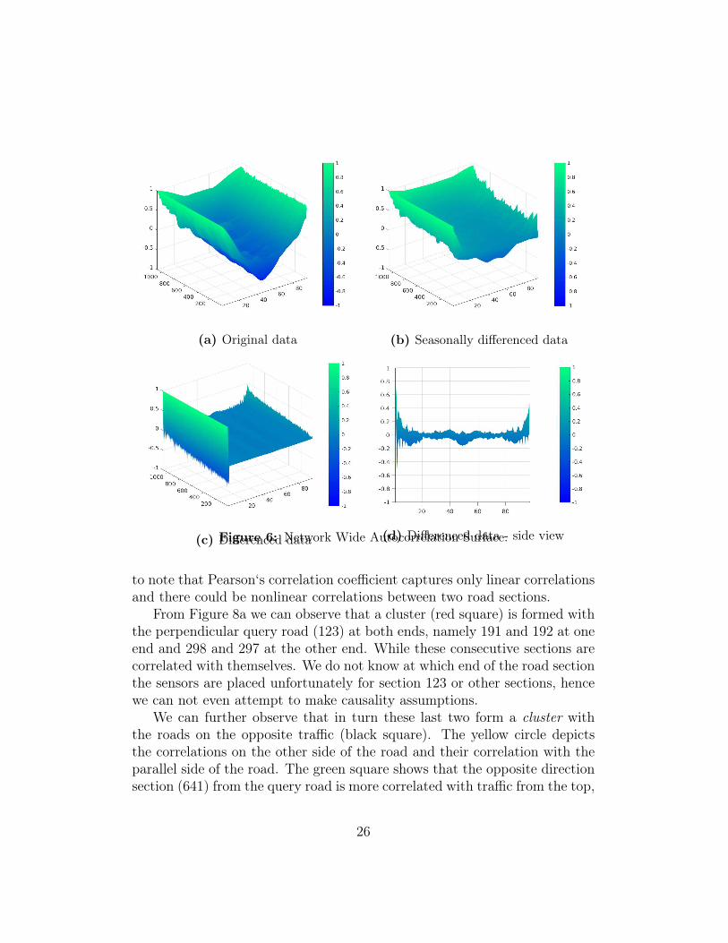
(a) Original data (b) Seasonally differenced data
(c) Differenced data (d) Differenced data - side viewFigure 6: Network Wide Autocorrelation Surface.
to note that Pearson‘s correlation coefficient captures only linear correlationsand there could be nonlinear correlations between two road sections.
From Figure 8a we can observe that a cluster (red square) is formed withthe perpendicular query road (123) at both ends, namely 191 and 192 at oneend and 298 and 297 at the other end. While these consecutive sections arecorrelated with themselves. We do not know at which end of the road sectionthe sensors are placed unfortunately for section 123 or other sections, hencewe can not even attempt to make causality assumptions.
We can further observe that in turn these last two form a cluster withthe roads on the opposite traffic (black square). The yellow circle depictsthe correlations on the other side of the road and their correlation with theparallel side of the road. The green square shows that the opposite directionsection (641) from the query road is more correlated with traffic from the top,
26

145.03 145.035 145.04 145.045 145.05 145.055
-37.875
-37.87
-37.865
-37.86
-37.855
Sensor 123 - Connected roads and correlations with S123
122 [0.89]
191 [0.9]
192 [0.94]
297 [0.91]
298 [0.93]
640 [0.69]
641 [0.77]
642 [0.77]
708 [0.75]
709 [0.83]
804 [0.86]
805 [0.88]
(a) Sensor 123 - directly connected roads
145.05 145.052 145.054 145.056 145.058 145.06 145.062 145.064 145.066
-37.866
-37.864
-37.862
-37.86
-37.858
-37.856
-37.854
-37.852
Sensor 4 - Adjacent roads according to mean euclidean distance
240 [0.76]
753 [0.62]
241 [0.91]
752 [0.42]
730 [0.57]
239 [0.79]
754 [0.48]
215 [0.77]
731 [0.43]
296 [0.73]
806 [0.63]
522 [0.62]295 [0.73]
(b) Sensor 4 - nearest via euclidean dis-tance
Figure 7: Road sections are marked for either direction (unreliable).
(a) Sensor 123 (b) Sensor 4
Figure 8: Correlation matrix for two different road sections
bottom and left side. Upon even more careful inspection, these correlationsreveal the behaviour of traffic despite the fact that we are unaware of theactual direction of traffic – we are looking at an undirected graph.
Conversely, in Figure 8b we can observe that there are clusters formedfor the other road segments while segment 4 is only slightly correlated withsection 241. Nevertheless, there are still weak correlations even at this rel-
27

atively isolated location. Figure 7 shows that it is not necessary for a roadsection to have direct adjacent road sections. However, the traffic volume onthis road is still influenced by the nearby on and off ramps. Hence, we plotin Figure 7b the closest road sections using the euclidean distance. Recentwork optimize only for individual series forecasting and hence does not takeproximity data into consideration towards making predictions (Lippi et al.,2013), an observation also made by the authors. It is evident that there aredependencies between sensors in a traffic network, especially at intersectionsas we show in Figure 8.
Thus far we have observed proximity operators based on direct adjacentconnections or euclidean distance. We use the correlation as a metric forselecting road sections as opposed to using the map coordinates for eachsensor. In Figure 9 we show that the top most correlated roads for these twosensors are not necessarily in the immediate neighbourhood. Therefore, thisis not a reliable means of selecting additional relevant data for the predictors,since it is quite unlikely that there are dependencies between road sectionsthat are far apart. Perhaps a better way of selection is to compute thecross-correlation over a fixed window interval, which accounts for shifts inthe traffic signal.
145 145.02 145.04 145.06 145.08 145.1 145.12
-37.91
-37.9
-37.89
-37.88
-37.87
-37.86
-37.85
-37.84
-37.83
-37.82
-37.81
Sensor 123 - Highest ranked sensors according to correlation
851 [0.96]
1024 [0.96]
6 [0.96]
852 [0.95]
(a) Sensor 123
144.96 144.98 145 145.02 145.04 145.06 145.08 145.1
-37.88
-37.86
-37.84
-37.82
-37.8
-37.78
Sensor 4 - Highest ranked sensors according to correlation
241 [0.91]
255 [0.89]254 [0.89]
242 [0.88]
(b) Sensor 4
Figure 9: Ranked road sections by correlation. Query is solid black. The highestranked are shown in dotted black. There is a large distance between the query andthe highest correlated over the entire dataset.
The correlations for all sensors in one area are shown in Figure 8. Clearly,
28

the road section 123 has much more correlated traffic than the off highwayramp (section 4). This is due to the fact that the ramp has no actual con-nected roads and we selected these roads using the euclidean distance matrix.The implications are evident: there is valuable information carried within theneighbourhood of each query road section where predictions are to be made.
Previous research has shown that separating prediction on working andnon-working (weekends) days can improve performance if independent pre-dictors are deployed separately for weekends or each day of the week. Addi-tionally, both a larger temporal context through a larger lag and includingproximity data can increase prediction accuracy (Schimbinschi et al., 2015).
4.6. Pair-wise correlations with query station as a function of time
We further investigate whether the interactions depicted in Figure 8change during the day. In the following figure we can observe that theseindeed change. There is an overall pattern, however most importantly thereare deviations from the standard pattern such as the sudden spikes at 4 amfor the blue sensor station and the spike at 6pm for the green sensor station.
12AM
1AM
2AM
3AM
4AM
5AM
6AM
7AM
8AM
9AM
10AM
11AM
12PM
1PM
2PM
3PM
4PM
5PM
6PM
7PM
8PM
9PM
10PM
11PM
0.1
0.2
0.3
0.4
0.5
0.6
0.7
0.8
Co
rre
latio
n
Sensor 123 topological Pearson correlations @ time of day
122
124
191
192
297
298
640
641
642
708
709
804
805
Figure 10: Sensor 123 correlation at time of day with neighboring sensors
5. Results and discussion
In this section we evaluate the network wide prediction performance forthe two datasets and compare univariate methods to Topology Regularized
29

Vector Autoregression (TRU-VAR) generalized to state of the art functionapproximators. In all experiments we only report the error of ex-ante pointforecasts, in other words, no information that would not be available at thetime of prediction was used in any of the experiments.
5.1. Experimental setup
For all experiments the data was split sequentially into 70% training 15%validation and 15% testing. Preparation of data is discussed in Section 4. Inthe case of ARIMA, the models were fit on the training plus validation data.The regularization parameters and the fitting of the ARIMA (using the fore-cast package in R (Hyndman et al., 2007)) were found independently for eachsensor station. The MLPs are trained using the gauss-newton approximationfor bayesian L2 regularized backpropagation (Foresee & Hagan, 1997). In thecase of the LLS and SVR we use L-BFGS (Nocedal & Wright, 2006, ch. 9)for ridge and SPARSA (Wright et al., 2009) for LASSO regularization.
As a follow-up on the observations made in Figure 8a and Figure 8b wepropose learning Topology Regularized Universal Vector Autoregression byinducing sparsity in the VAR model, in effect including only relevant datafrom the nearby roads to each autoregressor. However, not all road sectionshave direct connections. For the VicRoads dataset, we only use data fromthe directly connected roads, if the road section has direct connections. InFigure 7b the nearest roads for road section 4 are plotted, however thereare no directly connected roads, a case where no additional data is added.In this case, the topological adjacency matrix can be refined according toother heuristics for selecting relevant roads, as discussed in Section 3. PeMSis very sparse given the area covered, we take the closest K = 6 roads asadditional data, computed using the graph adjacency matrix from the mapGPS coordinate of each sensor. We empirically selected K based on the outof sample (test set) mean RMSE using univariate OLS fitting.
We set a naive baseline using the CMSD as specified in Section 4, whichis the average specific to the time of day, sensor and day of the week. Wefurthermore compare these methods with ARIMA which is also an intuitivebaseline. Note that we do not provide comparisons with VAR since this wouldbe computationally prohibitive, expecially for the VicRoads dataset wherethe input space would have almost 10k (∆ = 10 × 1084) dimensions, justfor one vector. We do not perform direct comparisons with recent methods(Ko et al., 2016; Salamanis et al., 2016; Wu et al., 2016; Ahn et al., 2015;Fusco et al., 2015; Lv et al., 2015; Xu et al., 2015) since: 1) this would
30

be computationally prohibitive – in the original articles, most authors donot perform network-wide experiments and we have a dataset with 1000+sensor stations; 2) these methods do not have the properties described inthe introduction (Table 1 on 4); 3) we aim for a direct comparison over theunivariate equivalent of the function approximator used within TRU-VAR.
Univariate models and TRU-VAR are compared via the average RMSEand MAPE for both datasets.
5.2. Choosing the lag order
We train a linear TRU-VAR over increasing lag windows ∆ ∈ 1, 2, 3, 5 . . . , 31and plot the validation set RMSE and computation time, towards makingan empirical choice for the lag value. A larger lag decreases prediction error,while putting a heavier load on processing time. As a tradeoff we set ∆ = 10and use the same lag value for the VicRoads dataset.
1 3 5 7 9 11 13 15 17 19 21 23 25 27 29 31
Lag
5
5.1
5.2
5.3
5.4
5.5
5.6
5.7
5.8
5.9
6
6.1
6.2
RM
SE
Error
1 3 5 7 9 11 13 15 17 19 21 23 25 27 29 31
Lag
0
10
20
30
40
50
60
Tim
e (
seconds)
Speed
Figure 11: RMSE and prediction time as a function of lag (PeMS).
Using this procedure we aim to get an estimate of the out of sample error.We also mention that using this lag value the error on the test set is lower formodels with the same lag value as oppossed to the ARIMA forecasts wherethe lags were selected automatically for each timeseries based on the AIC.It is however likely that if optimizing the lag values in the same way forTRU-VAR, the error could be further lowered.
5.3. TRU-VAR vs. Univariate
It can be observed from Table 2 that TRU-VAR outperformed the uni-variate methods in all cases except for SVR-L1.
31

Table 2: VicRoads dataset - Average RMSETopology regularized universal vector autoregression (TRU-VAR)outperforms univariate models for all f except SVR-L1.
f(x) OLS LLS-L1 LLS-L2 SVR-L1 SVR-L2 MLP-L2
Univariate 24.11 24.13 24.37 24.94 24.51 22.09
± 15.4 ± 15.4 ± 15.5 ± 15.9 ± 15.9 ± 15.6
TRU-VAR 22.64 23.14 22.93 26.68 22.78 21.36
± 15.6 ± 15.7 ± 15.4 ± 18.5 ± 15.1 ± 15.3
Baselines CMSD: 35.29 ± 29.0 ARIMA: 24.32 ± 15.6
Table 3: VicRoads dataset - Average MAPE Topology regularized universalvector autoregression (TRU-VAR)outperforms univariate models for all f except SVR-L1.
f(x) OLS LLS-L1 LLS-L2 SVR-L1 SVR-L2 MLP-L2
Univariate 26.94 27.14 28.42 28.22 27.56 21.27
± 12.4 ± 12.6 ± 14.2 ± 14.6 ± 14.6 ± 8.5
TRU-VAR 22.96 24.53 24.16 31.91 24.28 21.03
± 9.9 ± 13.8 ± 12.5 ± 26.3 ± 13.7 ± 11.7
Baselines CMSD: 32.86 ± 53.4 ARIMA: 27.91 ± 13.4
For PeMS there are usually just two adjacent sensors (upstream anddownstream) which can contribute to the traffic volume. We were unableto pinpoint the start and end location of the road section covered by thesensor station unlike VicRoads. Since we only had the GPS coordinates ofstations themselves, we defined the TDAM based on the euclidean distance tothe query sensor station. This usually resulted in includin the sensor stationson the opposite direction of traffic. While this helps in the case of VicRoads,for freeways the traffic is strictly separated between traffic directions, henceit is not relevant and adds unecessary complexity. However, it is interestingthat we were able to lower the prediction error by defining the adjacencymatrix based on the K roads furtherest apart from the prediction location
32

for the OLS and MLP. The results are shown in Table 4 in the last row. Fromthe same table it can be seen that for higher temporal resolutions such asin the case of PeMS, the lowest errors are recorded via OLS and MLP whileARIMA, LLS and SVR show higher error.
Table 4: PeMS dataset - Average RMSETopology regularized universal vector autoregression (TRU-VAR)outperforms univariate models for all f except LLS-L1.
f(x) OLS LLS-L1 LLS-L2 SVR-L1 SVR-L2 MLP-L2
Univariate 4.61 4.64 4.97 5.20 4.72 4.55
± 2.1 ± 2.0 ± 2.4 ± 2.6 ± 2.0 ± 2.0
TRU-VAR 4.53 4.64 4.92 5.03 4.70 4.45
± 2.0 ± 2.1 ± 2.5 ± 2.7 ± 2.0 ± 1.9
Baselines CMSD: 5.16 ± 3.1 ARIMA: 4.67 ± 1.7
Table 5: PeMS dataset - Average MAPETopology regularized universal vector autoregression (TRU-VAR)outperforms univariate models for all f except LLS-L1.
f(x) OLS LLS-L1 LLS-L2 SVR-L1 SVR-L2 MLP-L2
Univariate 37.77 38.37 45.12 42.80 38.53 37.48
± 9.4 ± 11.0 ± 15.9 ± 20.4 ± 13.5 ± 9.8
TRU-VAR 36.95 38.37 41.59 39.74 37.69 37.42
± 10.3 ± 12.5 ± 14.7 ± 14.5 ± 12.3 ± 12.6
Baselines CMSD: 41.9 ± 19.2 ARIMA: 38.09 ± 15.76
5.4. Long-term forecasting: increasing the prediction horizon
In the previous section we shoed that TRU-VAR outperforms univariatemethods across different machine learning function approximation models.We now ask if this holds for larger prediction horizons for to up to twohours. Consequently, we compare the prediction performance of TRU-VAR
33

and univariate models with the two best performing models from the previ-ous section (OLS and MLP). The experiment is identical to the one in theprevious section, with the exception that now, instead of predicting at theimmediate step in the future (e.g. h = 1) we set the target variable to befurther in time. In other words, methods are idential data split is identical,input data is the same while the target variable changes.
Therefore, in the following section we show how the overall network errorrises as the prediction horizon is increased to up to two hours. We now referthe reader to Eq. 1 on page 14 for the definition of the prediction horizon.The horizon temporal resolution for t+h where h = 1 was initially 5 minutesfor PeMS and 15 minutes for VicRoads which correspond to the temporalresolution of the dataset.
Instead of predicting the volume of traffic at t+1 (for all series) we insteadtrain and subsequently evaluate the prediction error at horizons for up totwo hours. For PeMS, which has a resolution of 5 minutes per observationwe plot the error for eight 5-minute distanced horizons and then add 15-minute horizons up to two hours (we skip a few horizons) – this is visible inFigure 12a. For VicRoads the resolution is 15 minutes thus we only plot 8forecasts to reach the two hour goal (Figure 12b). Therefore, to evaluate allhorizons for up to two hours we require to fit h ∈ 1, 2, . . . , 8 models forVicRoads and h ∈ 1, 2, . . . , 24 for PeMS. However, for PeMS we skip a fewevaluations and take h ∈ 1, 2, 3, . . . , 8 ∪ 9, 12, . . . , 24.
Results are displayed in Figure 12 where the network-mean RMSE isdepicted with solid lines and the standard deviation with dotted lines as anindication of the network-spread of the error. It is evident that it is morechallenging to make predictions further in time, and it can be seen that theerror increases linearly as the prediction horizon is increased.
From both figures we can observe that TRU-VAR MLP predicts with thelowest error even as the forecasting horizon is increased, while the Univari-ate MLP (one simple neural network per timeseries) is the worst for bothdatasets. As the prediction horizon is moved further ahead in time not onlythe mean RMSE increases, but the spread of the error over the network alsoincreases. For PeMS the error increases by approximately 36% when thehorizon is moved from five minutes to two hours (for TRU-VAR MLP) whilefor VicRoads, the error increases by 97%. This is to be expected for a muchlarger network, with a more complex topology, a greater variety of road typesand a lower temporal resolution.
Overall, the error spread appears to be much more stable for PeMS and
34

5 10 15 20 25 30 35 40 45 60 75 90 105 120
Horizon (minutes)
2
4
6
8
10
12
14
RM
SE
(vehic
les)
TRU-VAR MLP
TRU-VAR OLS
Univariate MLP
Univariate OLS
(a) PeMS
15 30 45 60 75 90 105 120
Horizon (minutes)
0
20
40
60
80
100
120
RM
SE
(vehic
les)
TRU-VAR MLP
TRU-VAR OLS
Univariate MLP
Univariate OLS
(b) VicRoads
Figure 12: Behavior of error when prediction horizon is increased. µ RMSE withsolid lines and spread of µ ± σ RMSE with dotted lines. Lower is better, errorincreases linearly with the prediction horizon.
the OLS approximators. This is for two reasons: 1) VicRoads has 10 timesmore sensor stations, which can cause a much larger error spread; 2) for theMLP experiments we trained the neural networks using first order gradientmethods which was faster, however less stable than when using bayesianregularization as in the previous experiments in Table 2.
6. Conclusions and future work
In the current article we defined necessary properties for large scale net-work wide traffic forecasting in the context of growing urban road networksand (semi)autonomous vehicles. We performed a broad review of the litera-ture and after drawing conclusions, we discussed data quality, preprocessingand provided suggestions for defining a topology-designed adjacency matrix(TDAM).
We consequently proposed topology-regularized universal vector autore-gression (TRU-VAR). We compared the network-wide prediction error ofthe univariate and TRU-VAR prediction models over two quantitatively andqualitatively different datasets. TRU-VAR outperforms the CMSD baselineand ARIMA in all cases and the regularized univariate models in almost allcases. For VicRoads, which has high spatial but relatively lower temporal
35

resolution, TRU-VAR outperformed the univariate method in all cases ex-cept for SVR-L1. For the PeMS dataset, TRU-VAR showed lower error inall cases except for LLS-L1. From the prediction horizon experiments (Fig-ure 12) we concluded that the TRU-VAR MLP approximator has the lowesterror even when the forecast horizon is increased up to two hours, for bothdatasets.
PeMS was easier to predict and the RMSE is lower than for VicRoads.We would like to remind the reader that approximately half of the sensorstations in the VicRoads dataset can have more than 50% data missing. Wedid not remove these from the model. This evidently increases the overallerror. At the same time, the PeMS dataset has higher temporal resolution(5 vs 15 minutes) however it is much smaller and has 10 times less sensorstations. With continuous state-space models and accounting for the spatialsparsity (large distance between sensor stations on highways causes shifts inthe signals) the error could be further decreased.
We conclude that the TDAM is a key component to our proposed trafficforecasting expert system since it has a great impact on prediction accuracyand should be tailored to the type of road network using expert domainknowledge heuristics. Therefore, the weak points of our method also residein its strengths, namely: the design of the topological adjacency matrix isvery important and is subject to domain knowledge; the model customiza-tion flexibility allows for a large search space of possibilities which can beoverwhelming to fine-tune, if required. When designing the adjacency matrixfor the VicRoads dataset, we could have opted to rank the most correlatedconnected ones and select the top K ranked ones, in this way having anequal number of additional streams for each prediction point. For the roadswithout direct connections, this would require computing the distance to theclosest roads based on the euclidean distance and performing a correlationranking. This could further increase accuracy since for some sensors (for ex-ample highway off ramps) there are no directly connected roads, hence simpleregression is performed. An alternative would have been to select second or-der connections for the stations with a low graph node degree, such that ofhighway off ramps. We leave this for future work, also aiming to investigatecontinuous state space models, multi-metric data and other multi-task learn-ing architectures. Moreover, we also aim to show that including temporalfeatures and adding multi-metric data (such as vehicle-crowdsourced data)can further increase prediction performance.
Finally, we would like to point out that our method can be trained online,
36

can have a nonlinear reporesentation, has a low complexity due to the topo-logical constraints, is non-static and robust towards changes (data sourcesor structure) thus scales well, is efficient and easy to redeploy. Given thatthe error increases linearly within reasonable bounds (Fig. 12) for up to twohours, our method may be useful in other contexts and applications otherthan road traffic, such as natural disaster prevention (e.g. river flood fore-casting), telecommunications (e.g. antenna load forecasts), networking (e.g.forecasts for routing), finance to name a few. In general, the method can beapplied to any type of dataset consisting of multivariate timeseries, where theconstraints are known a priori or can be inferred from the data to constructthe topology matrix.
References
Abdulhai, B., Porwal, H., & Recker, W. (2002). Short-term traffic flowprediction using neuro-genetic algorithms. ITS Journal-Intelligent Trans-portation Systems Journal , 7 , 3–41.
Ahn, J. Y., Ko, E., & Kim, E. (2015). Predicting spatiotemporal traffic flowbased on support vector regression and bayesian classifier. In Big Data andCloud Computing (BDCloud), 2015 IEEE Fifth International Conferenceon (pp. 125–130). IEEE.
Asif, M. T., Dauwels, J., Goh, C. Y., Oran, A., Fathi, E., Xu, M., Dhanya,M. M., Mitrovic, N., & Jaillet, P. (2014). Spatiotemporal patterns in large-scale traffic speed prediction. IEEE Transactions on Intelligent Trans-portation Systems, 15 , 794–804.
Athanasopoulos, G., Poskitt, D., & Vahid, F. (2012). Two canonical varmaforms: Scalar component models vis-à-vis the echelon form. EconometricReviews , 31 , 60–83.
Au, T.-C., Zhang, S., & Stone, P. (2015). Autonomous intersection manage-ment for semi-autonomous vehicles. Handbook of Transportation. Rout-ledge, Taylor & Francis Group, .
Blue, V., List, G. F., & Embrechts, M. J. (1994). Neural net freeway traveltime estimation. In Intelligent Engineering Systems through Artificial Neu-ral Networks (Conference: 1994: Saint Louis, Mo.). Proceedings. Vol. 4 .
37

Box, G. E., Jenkins, G. M., Reinsel, G. C., & Ljung, G. M. (2015). Timeseries analysis: forecasting and control . John Wiley & Sons.
Castillo, E., Menéndez, J. M., & Sánchez-Cambronero, S. (2008). Predict-ing traffic flow using bayesian networks. Transportation Research Part B:Methodological , 42 , 482–509.
Castro-Neto, M., Jeong, Y.-S., Jeong, M.-K., & Han, L. D. (2009). Online-svr for short-term traffic flow prediction under typical and atypical trafficconditions. Expert systems with applications, 36 , 6164–6173.
Çetiner, B. G., Sari, M., & Borat, O. (2010). A neural network based traffic-flow prediction model. Mathematical and Computational Applications, 15 ,269–278.
Chai, T., & Draxler, R. R. (2014). Root mean square error (rmse) or meanabsolute error (mae)?–arguments against avoiding rmse in the literature.Geoscientific Model Development , 7 , 1247–1250.
Chen, C., Hu, J., Meng, Q., & Zhang, Y. (2011). Short-time traffic flow pre-diction with arima-garch model. In Intelligent Vehicles Symposium (IV),2011 IEEE (pp. 607–612). IEEE.
Cheng, T., Haworth, J., & Wang, J. (2012). Spatio-temporal autocorrelationof road network data. Journal of Geographical Systems, 14 , 389–413.
Clark, S. (2003). Traffic prediction using multivariate nonparametric regres-sion. Journal of transportation engineering , 129 , 161–168.
Clark, S. D., Dougherty, M. S., & Kirby, H. R. (1993). The use of neuralnetworks and time series models for short term traffic forecasting: a com-parative study. In Transportation Planning Methods. Proceedings Of Semi-nar D Held At The Ptrc European Transport, Highways And Planning 21stSummer Annual Meeting (September 13-17, 1993), Umist. Volume P363 .
Çolak, S., Lima, A., & González, M. C. (2016). Understanding congestedtravel in urban areas. Nature communications, 7 .
Cybenko, G. (1989). Approximation by superpositions of a sigmoidal func-tion. Mathematics of control, signals and systems, 2 , 303–314.
38

Dia, H. (2001). An object-oriented neural network approach to short-termtraffic forecasting. European Journal of Operational Research, 131 , 253–261.
Diebold, F. X., & Mariano, R. S. (2012). Comparing predictive accuracy.Journal of Business & economic statistics, .
Domingos, P. (2012). A few useful things to know about machine learning.Communications of the ACM , 55 , 78–87.
Dougherty, M. S., & Cobbett, M. R. (1997). Short-term inter-urban trafficforecasts using neural networks. International journal of forecasting , 13 ,21–31.
Foresee, F. D., & Hagan, M. T. (1997). Gauss-newton approximation tobayesian learning. In Neural Networks, 1997., International Conferenceon (pp. 1930–1935). IEEE volume 3.
Fusco, G., Colombaroni, C., Comelli, L., & Isaenko, N. (2015). Short-termtraffic predictions on large urban traffic networks: applications of network-based machine learning models and dynamic traffic assignment models. InModels and Technologies for Intelligent Transportation Systems (MT-ITS),2015 International Conference on (pp. 93–101). IEEE.
Guidotti, R., Nanni, M., Rinzivillo, S., Pedreschi, D., & Giannotti, F. (2016).Never drive alone: Boosting carpooling with network analysis. InformationSystems , .
Hamilton, J. D. (1994). Time series analysis volume 2. Princeton universitypress Princeton.
Högberg, P. (1976). Estimation of parameters in models for traffic prediction:a non-linear regression approach. Transportation Research, 10 , 263–265.
Hong, H., Huang, W., Xing, X., Zhou, X., Lu, H., Bian, K., & Xie, K.(2015). Hybrid multi-metric k-nearest neighbor regression for traffic flowprediction. In 2015 IEEE 18th International Conference on IntelligentTransportation Systems (pp. 2262–2267). IEEE.
Hyndman, R. J., Khandakar, Y. et al. (2007). Automatic time series for fore-casting: the forecast package for R. Technical Report Monash University,Department of Econometrics and Business Statistics.
39

Jensen, T., & Nielsen, S. (1973). Calibrating a gravity model and estimatingits parameters using traffic volume counts. In 5th Conference of Universi-ties’ Transport Study Groups, University College, London.
Kachroo, P., & Sastry, S. (2016). Traffic assignment using a density-basedtravel-time function for intelligent transportation systems. IEEE Transac-tions on Intelligent Transportation Systems, 17 , 1438–1447.
Kamarianakis, Y., & Prastacos, P. (2005). Space–time modeling of trafficflow. Computers & Geosciences, 31 , 119–133.
Kamarianakis, Y., Shen, W., & Wynter, L. (2012). Real-time road trafficforecasting using regime-switching space-time models and adaptive lasso.Applied Stochastic Models in Business and Industry , 28 , 297–315.
Karlaftis, M. G., & Vlahogianni, E. I. (2011). Statistical methods versusneural networks in transportation research: Differences, similarities andsome insights. Transportation Research Part C: Emerging Technologies,19 , 387–399.
Ko, E., Ahn, J., & Kim, E. Y. (2016). 3d markov process for traffic flowprediction in real-time. Sensors , 16 , 147.
Kumar, S. V., & Vanajakshi, L. (2015). Short-term traffic flow predictionusing seasonal arima model with limited input data. European TransportResearch Review , 7 , 1–9.
Lee, E.-M., Kim, J.-H., & Yoon, W.-S. (2007). Traffic speed predictionunder weekday, time, and neighboring links’ speed: back propagation neu-ral network approach. In Advanced Intelligent Computing Theories andApplications. With Aspects of Theoretical and Methodological Issues (pp.626–635). Springer.
Levin, M., & Tsao, Y.-D. (1980). On forecasting freeway occupancies andvolumes (abridgment). Transportation Research Record , .
Liebig, T., Piatkowski, N., Bockermann, C., & Morik, K. (2016). Dynamicroute planning with real-time traffic predictions. Information Systems, .
Lippi, M., Bertini, M., & Frasconi, P. (2013). Short-term traffic flow forecast-ing: An experimental comparison of time-series analysis and supervised
40

learning. Intelligent Transportation Systems, IEEE Transactions on, 14 ,871–882.
Low, D. E. (1972). A new approach to transportation systems modeling.Traffic quarterly , 26 .
Lütkepohl, H. (2005). New introduction to multiple time series analysis.Springer Science & Business Media.
Lv, Y., Duan, Y., Kang, W., Li, Z., & Wang, F.-Y. (2015). Traffic flow predic-tion with big data: A deep learning approach. Intelligent TransportationSystems, IEEE Transactions on, 16 , 865–873.
Lv, Y., Tang, S., & Zhao, H. (2009). Real-time highway traffic accidentprediction based on the k-nearest neighbor method. In 2009 InternationalConference on Measuring Technology and Mechatronics Automation (pp.547–550). IEEE volume 3.
Min, W., & Wynter, L. (2011). Real-time road traffic prediction with spatio-temporal correlations. Transportation Research Part C: Emerging Tech-nologies , 19 , 606–616.
Min, X., Hu, J., Chen, Q., Zhang, T., & Zhang, Y. (2009). Short-termtraffic flow forecasting of urban network based on dynamic starima model.In 2009 12th International IEEE Conference on Intelligent TransportationSystems (pp. 1–6). IEEE.
Mitrovic, N., Asif, M. T., Dauwels, J., & Jaillet, P. (2015). Low-dimensionalmodels for compressed sensing and prediction of large-scale traffic data.IEEE Transactions on Intelligent Transportation Systems, 16 , 2949–2954.
Moreira-Matias, L., & Alesiani, F. (2015). Drift3flow: Freeway-incident pre-diction using real-time learning. In 2015 IEEE 18th International Confer-ence on Intelligent Transportation Systems (pp. 566–571). IEEE.
Moreira-Matias, L., Gama, J., Ferreira, M., Mendes-Moreira, J., & Damas,L. (2016). Time-evolving od matrix estimation using high-speed gps datastreams. Expert Systems With Applications, 44 , 275–288.
Murphy, K. P. (2012). Machine learning: a probabilistic perspective.
41

Nocedal, J., & Wright, S. (2006). Numerical optimization. Springer Science& Business Media.
Oh, S., Byon, Y.-J., Jang, K., & Yeo, H. (2015). Short-term travel-timeprediction on highway: a review of the data-driven approach. TransportReviews , 35 , 4–32.
Park, J., Li, D., Murphey, Y. L., Kristinsson, J., McGee, R., Kuang, M., &Phillips, T. (2011). Real time vehicle speed prediction using a neural net-work traffic model. In Neural Networks (IJCNN), The 2011 InternationalJoint Conference on (pp. 2991–2996). IEEE.
Rice, J., & Van Zwet, E. (2004). A simple and effective method for predictingtravel times on freeways. IEEE Transactions on Intelligent TransportationSystems , 5 , 200–207.
Salamanis, A., Kehagias, D. D., Filelis-Papadopoulos, C. K., Tzovaras, D.,& Gravvanis, G. A. (2016). Managing spatial graph dependencies in largevolumes of traffic data for travel-time prediction. IEEE Transactions onIntelligent Transportation Systems, 17 , 1678–1687.
Schimbinschi, F., Nguyen, X. V., Bailey, J., Leckie, C., Vu, H., & Kotagiri, R.(2015). Traffic forecasting in complex urban networks: Leveraging big dataand machine learning. In Big Data (Big Data), 2015 IEEE InternationalConference on (pp. 1019–1024). IEEE.
Smith, B. L., & Demetsky, M. J. (1997). Traffic flow forecasting: comparisonof modeling approaches. Journal of transportation engineering , 123 , 261–266.
Smith, B. L., Williams, B. M., & Oswald, R. K. (2002). Comparison ofparametric and nonparametric models for traffic flow forecasting. Trans-portation Research Part C: Emerging Technologies , 10 , 303–321.
Smola, A., & Vapnik, V. (1997). Support vector regression machines. Ad-vances in neural information processing systems, 9 , 155–161.
Stathopoulos, A., Dimitriou, L., & Tsekeris, T. (2008). Fuzzy modelingapproach for combined forecasting of urban traffic flow. Computer-AidedCivil and Infrastructure Engineering , 23 , 521–535.
42

Stathopoulos, A., & Karlaftis, M. G. (2003). A multivariate state spaceapproach for urban traffic flow modeling and prediction. TransportationResearch Part C: Emerging Technologies, 11 , 121–135.
Su, F., Dong, H., Jia, L., Qin, Y., & Tian, Z. (2016). Long-term forecastingoriented to urban expressway traffic situation. Advances in MechanicalEngineering , 8 , 1687814016628397.
Suykens, J. A., & Vandewalle, J. (1999). Least squares support vector ma-chine classifiers. Neural processing letters, 9 , 293–300.
Szeto, W., Ghosh, B., Basu, B., & O’Mahony, M. (2009). Multivariate traf-fic forecasting technique using cell transmission model and sarima model.Journal of Transportation Engineering , 135 , 658–667.
Tibshirani, R. (1996). Regression shrinkage and selection via the lasso. Jour-nal of the Royal Statistical Society. Series B (Methodological), (pp. 267–288).
Van Lint, J., & Van Hinsbergen, C. (2012). Short-term traffic and travel timeprediction models. Artificial Intelligence Applications to Critical Trans-portation Issues, 22 , 22–41.
Vapnik, V. N. (1999). An overview of statistical learning theory. IEEEtransactions on neural networks, 10 , 988–999.
Varaiya, P. P. (2001). Freeway performance measurement system: Final re-port . Citeseer.
Vlahogianni, E. I., Golias, J. C., & Karlaftis, M. G. (2004). Short-term trafficforecasting: Overview of objectives and methods. Transport reviews , 24 ,533–557.
Vlahogianni, E. I., Karlaftis, M. G., & Golias, J. C. (2005). Optimized andmeta-optimized neural networks for short-term traffic flow prediction: agenetic approach. Transportation Research Part C: Emerging Technologies,13 , 211–234.
Vlahogianni, E. I., Karlaftis, M. G., & Golias, J. C. (2014). Short-term trafficforecasting: Where we are and where we’re going. Transportation ResearchPart C: Emerging Technologies, 43 , 3–19.
43

Wang, Y., Papageorgiou, M., & Messmer, A. (2008). Real-time freeway trafficstate estimation based on extended kalman filter: Adaptive capabilities andreal data testing. Transportation Research Part A: Policy and Practice,42 , 1340–1358.
Williams, B. (2001). Multivariate vehicular traffic flow prediction: evalua-tion of arimax modeling. Transportation Research Record: Journal of theTransportation Research Board , (pp. 194–200).
Wright, S. J., Nowak, R. D., & Figueiredo, M. A. (2009). Sparse reconstruc-tion by separable approximation. IEEE Transactions on Signal Processing ,57 , 2479–2493.
Wu, C.-H., Ho, J.-M., & Lee, D.-T. (2004). Travel-time prediction withsupport vector regression. IEEE transactions on intelligent transportationsystems , 5 , 276–281.
Wu, Y.-J., Chen, F., Lu, C.-T., & Yang, S. (2016). Urban traffic flow predic-tion using a spatio-temporal random effects model. Journal of IntelligentTransportation Systems, 20 , 282–293.
Xie, Y., Zhang, Y., & Ye, Z. (2007). Short-term traffic volume forecastingusing kalman filter with discrete wavelet decomposition. Computer-AidedCivil and Infrastructure Engineering , 22 , 326–334.
Xu, Y., Chen, H., Kong, Q.-J., Zhai, X., & Liu, Y. (2015). Urban traffic flowprediction: a spatio-temporal variable selection-based approach. Journalof Advanced Transportation, .
Zeng, D., Xu, J., Gu, J., Liu, L., & Xu, G. (2008). Short term traffic flowprediction based on online learning svr. In Power Electronics and Intelli-gent Transportation System, 2008. PEITS’08. Workshop on (pp. 616–620).IEEE.
Zhang, G. P. (2003). Time series forecasting using a hybrid arima and neuralnetwork model. Neurocomputing , 50 , 159–175.
Zheng, W., Lee, D.-H., & Shi, Q. (2006). Short-term freeway traffic flowprediction: Bayesian combined neural network approach. Journal of trans-portation engineering , 132 , 114–121.
44

Zou, H., & Hastie, T. (2005). Regularization and variable selection via theelastic net. Journal of the Royal Statistical Society: Series B (StatisticalMethodology), 67 , 301–320.
45