Topics in Fourier Analysis:

DFT&FFT,Wavelets, Laplace Transform

by Peter J. Olver

University of Minnesota

1. Introduction.

In addition to their inestimable importance in mathematics and its applications,Fourier series also serve as the entry point into the wonderful world of Fourier analy-sis and its wide-ranging extensions and generalizations. An entire industry is devoted tofurther developing the theory and enlarging the scope of applications of Fourier–inspiredmethods. New directions in Fourier analysis continue to be discovered and exploited ina broad range of physical, mathematical, engineering, chemical, biological, financial, andother systems. In this chapter, we will concentrate on four of the most important variants:discrete Fourier sums leading to the Fast Fourier Transform (FFT); the modern theoryof wavelets; the Fourier transform; and, finally, its cousin, the Laplace transform. In ad-dition, more general types of eigenfunction expansions associated with partial differentialequations in higher dimensions will appear in the following chapters.

Modern digital media, such as CD’s, DVD’s and MP3’s, are based on discrete data,not continuous functions. One typically samples an analog signal at equally spaced timeintervals, and then works exclusively with the resulting discrete (digital) data. The asso-ciated discrete Fourier representation re-expresses the data in terms of sampled complexexponentials; it can, in fact, be handled by finite-dimensional vector space methods, andso, technically, belongs back in the linear algebra portion of this text. However, the insightgained from the classical continuous Fourier theory proves to be essential in understand-ing and analyzing its discrete digital counterpart. An important application of discreteFourier sums is in signal and image processing. Basic data compression and noise removalalgorithms are applied to the sample’s discrete Fourier coefficients, acting on the obser-vation that noise tends to accumulate in the high frequency Fourier modes, while mostimportant features are concentrated at low frequencies. The first Section 2 develops thebasic Fourier theory in this discrete setting, culminating in the Fast Fourier Transform(FFT), which produces an efficient numerical algorithm for passing between a signal andits discrete Fourier coefficients.

One of the inherent limitations of classical Fourier methods, both continuous anddiscrete, is that they are not well adapted to localized data. (In physics, this lack oflocalization is the basis of the Heisenberg Uncertainty Principle.) As a result, Fourier-basedsignal processing algorithms tend to be inaccurate and/or inefficient when confrontinghighly localized signals or images. In the second section, we introduce the modern theoryof wavelets, which is a recent extension of Fourier analysis that more naturally incorporatesmultiple scales and localization. Wavelets are playing an increasingly dominant role in

10/3/17 1 c© 2017 Peter J. Olver

many modern applications; for instance, the new JPEG digital image compression formatis based on wavelets, as are the computerized FBI fingerprint data used in law enforcementin the United States.

The Laplace transform is a basic tool in engineering applications. To mathematicians,the Fourier transform is the more fundamental of the two, while the Laplace transformis viewed as a certain real specialization. Both transforms change differentiation intomultiplication, thereby converting linear differential equations into algebraic equations.The Fourier transform is primarily used for solving boundary value problems on the realline, while initial value problems, particularly those involving discontinuous forcing terms,are effectively handled by the Laplace transform.

2. Discrete Fourier Analysis and the Fast Fourier Transform.

In modern digital media — audio, still images or video — continuous signals aresampled at discrete time intervals before being processed. Fourier analysis decomposes thesampled signal into its fundamental periodic constituents — sines and cosines, or, moreconveniently, complex exponentials. The crucial fact, upon which all of modern signalprocessing is based, is that the sampled complex exponentials form an orthogonal basis.The section introduces the Discrete Fourier Transform, and concludes with an introductionto the Fast Fourier Transform, an efficient algorithm for computing the discrete Fourierrepresentation and reconstructing the signal from its Fourier coefficients.

We will concentrate on the one-dimensional version here. Let f(x) be a functionrepresenting the signal, defined on an interval a ≤ x ≤ b. Our computer can only store itsmeasured values at a finite number of sample points a ≤ x0 < x1 < · · · < xn ≤ b. In thesimplest and, by far, the most common case, the sample points are equally spaced, and so

xj = a+ j h, j = 0, . . . , n, where h =b− a

nindicates the sample rate. In signal processing applications, x represents time instead ofspace, and the xj are the times at which we sample the signal f(x). Sample rates can bevery high, e.g., every 10–20 milliseconds in current speech recognition systems.

For simplicity, we adopt the “standard” interval of 0 ≤ x ≤ 2π, and the n equallyspaced sample points†

x0 = 0, x1 =2π

n, x2 =

4π

n, . . . xj =

2j π

n, . . . xn−1 =

2(n− 1)π

n. (2.1)

(Signals defined on other intervals can be handled by simply rescaling the interval to havelength 2π.) Sampling a (complex-valued) signal or function f(x) produces the sample

vector

f =(f0, f1, . . . , fn−1

)T=(f(x0), f(x1), . . . , f(xn−1)

)T,

where

fj = f(xj) = f

(2j π

n

). (2.2)

† We will find it convenient to omit the final sample point xn = 2π from consideration.

10/3/17 2 c© 2017 Peter J. Olver

1 2 3 4 5 6

-1

-0.5

0.5

1

1 2 3 4 5 6

-1

-0.5

0.5

1

1 2 3 4 5 6

-1

-0.5

0.5

1

1 2 3 4 5 6

-1

-0.5

0.5

1

1 2 3 4 5 6

-1

-0.5

0.5

1

1 2 3 4 5 6

-1

-0.5

0.5

1

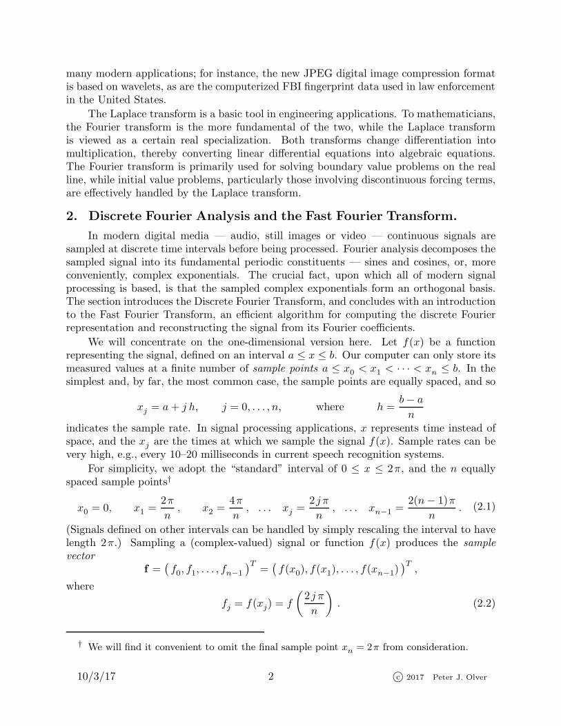
Figure 1. Sampling e− i x and e7 ix on n = 8 sample points.

Sampling cannot distinguish between functions that have the same values at all of thesample points — from the sampler’s point of view they are identical. For example, theperiodic complex exponential function

f(x) = e inx = cosnx+ i sinnx

has sampled values

fj = f

(2j π

n

)= exp

(in

2j π

n

)= e2j π i = 1 for all j = 0, . . . , n− 1,

and hence is indistinguishable from the constant function c(x) ≡ 1 — both lead to the

same sample vector ( 1, 1, . . . , 1 )T. This has the important implication that sampling at n

equally spaced sample points cannot detect periodic signals of frequency n. More generally,the two complex exponential signals

e i (k+n)x and e i kx

are also indistinguishable when sampled. This has the important consequence that weneed only use the first n periodic complex exponential functions

f0(x) = 1, f1(x) = e ix, f2(x) = e2 ix, . . . fn−1(x) = e(n−1) ix, (2.3)

in order to represent any 2π periodic sampled signal. In particular, exponentials e− i kx of“negative” frequency can all be converted into positive versions, namely e i (n−k)x, by thesame sampling argument. For example,

e− ix = cosx− i sinx and e(n−1) ix = cos(n− 1) x+ i sin(n− 1) x

have identical values on the sample points (2.1). However, off of the sample points, theyare quite different; the former is slowly varying, while the latter represents a high frequencyoscillation. In Figure 1, we compare e− ix and e7 ix when there are n = 8 sample values,indicated by the dots on the graphs. The top row compares the real parts, cosx and cos 7x,while the bottom row compares the imaginary parts, sinx and − sin 7x. Note that bothfunctions have the same pattern of sample values, even though their overall behavior isstrikingly different.

10/3/17 3 c© 2017 Peter J. Olver

This effect is commonly referred to as aliasing†. If you view a moving particle undera stroboscopic light that flashes only eight times, you would be unable to determine whichof the two graphs the particle was following. Aliasing is the cause of a well-known artifactin movies: spoked wheels can appear to be rotating backwards when our brain interpretsthe discretization of the high frequency forward motion imposed by the frames of thefilm as an equivalently discretized low frequency motion in reverse. Aliasing also hasimportant implications for the design of music CD’s. We must sample an audio signal ata sufficiently high rate that all audible frequencies can be adequately represented. In fact,human appreciation of music also relies on inaudible high frequency tones, and so a muchhigher sample rate is actually used in commercial CD design. But the sample rate that wasselected remains controversial; hi fi aficionados complain that it was not set high enoughto fully reproduce the musical quality of an analog LP record!

The discrete Fourier representation decomposes a sampled function f(x) into a linearcombination of complex exponentials. Since we cannot distinguish sampled exponentialsof frequency higher than n, we only need consider a finite linear combination

f(x) ∼ p(x) = c0 + c1 eix + c2 e

2 i x + · · · + cn−1 e(n−1) i x =

n−1∑

k=0

ck ei kx (2.4)

of the first n exponentials (2.3). The symbol ∼ in (2.4) means that the function f(x) andthe sum p(x) agree on the sample points:

f(xj) = p(xj), j = 0, . . . , n− 1. (2.5)

Therefore, p(x) can be viewed as a (complex-valued) interpolating trigonometric polynomial

of degree ≤ n− 1 for the sample data fj = f(xj).

Remark : If f(x) is real, then p(x) is also real on the sample points, but may very wellbe complex-valued in between. To avoid this unsatisfying state of affairs, we will usuallydiscard its imaginary component, and regard the real part of p(x) as “the” interpolatingtrigonometric polynomial. On the other hand, sticking with a purely real constructionunnecessarily complicates the analysis, and so we will retain the complex exponential form(2.4) of the discrete Fourier sum.

Since we are working in the finite-dimensional vector space Cn throughout, we mayreformulate the discrete Fourier series in vectorial form. Sampling the basic exponentials(2.3) produces the complex vectors

ωk =(e i kx0 , e i kx1 , e ikx2 , . . . , e ikxn−1

)T

=(1, e2kπ i /n, e4kπ i /n, . . . , e2(n−1)kπ i /n

)T,

k = 0, . . . , n− 1. (2.6)

† In computer graphics, the term “aliasing” is used in a much broader sense that covers avariety of artifacts introduced by discretization — particularly, the jagged appearance of linesand smooth curves on a digital monitor.

10/3/17 4 c© 2017 Peter J. Olver

The interpolation conditions (2.5) can be recast in the equivalent vector form

f = c0 ω0 + c1 ω1 + · · · + cn−1 ωn−1. (2.7)

In other words, to compute the discrete Fourier coefficients c0, . . . , cn−1 of f , all we needto do is rewrite its sample vector f as a linear combination of the sampled exponentialvectors ω0, . . . ,ωn−1.

Now, as with continuous Fourier series, the absolutely crucial property is the orthonor-mality of the basis elements ω0, . . . ,ωn−1. Were it not for the power of orthogonality,Fourier analysis might have remained a mere mathematical curiosity, rather than today’sindispensable tool.

Proposition 2.1. The sampled exponential vectors ω0, . . . ,ωn−1 form an orthonor-

mal basis of Cn with respect to the inner product

〈 f ; g 〉 =1

n

n−1∑

j=0

fj gj =1

n

n−1∑

j=0

f(xj) g(xj) , f , g ∈ Cn. (2.8)

Remark : The inner product (2.8) is a rescaled version of the standard Hermitian dotproduct between complex vectors. We can interpret the inner product between the samplevectors f , g as the average of the sampled values of the product signal f(x) g(x).

Remark : As usual, orthogonality is no accident. Just as the complex exponentialsare eigenfunctions for a self-adjoint boundary value problem, so their discrete sampledcounterparts are eigenvectors for a self-adjoint matrix eigenvalue problem. Here, though,to keep the discussion on track, we shall outline a direct proof.

Proof : The crux of the matter relies on properties of the remarkable complex numbers

ζn = e2π i /n = cos2π

n+ i sin

2π

n, where n = 1, 2, 3, . . . . (2.9)

Particular cases include

ζ2 = −1, ζ3 = − 12+

√32

i , ζ4 = i , and ζ8 =√22

+√22

i . (2.10)

The nth power of ζn is

ζnn =(e2π i /n

)n = e2π i = 1,

and hence ζn is one of the complex nth roots of unity : ζn = n√1. There are, in fact, n

different complex nth roots of 1, including 1 itself, namely the powers of ζn:

ζkn = e2 k π i /n = cos2 k π

n+ i sin

2 k π

n, k = 0, . . . , n− 1. (2.11)

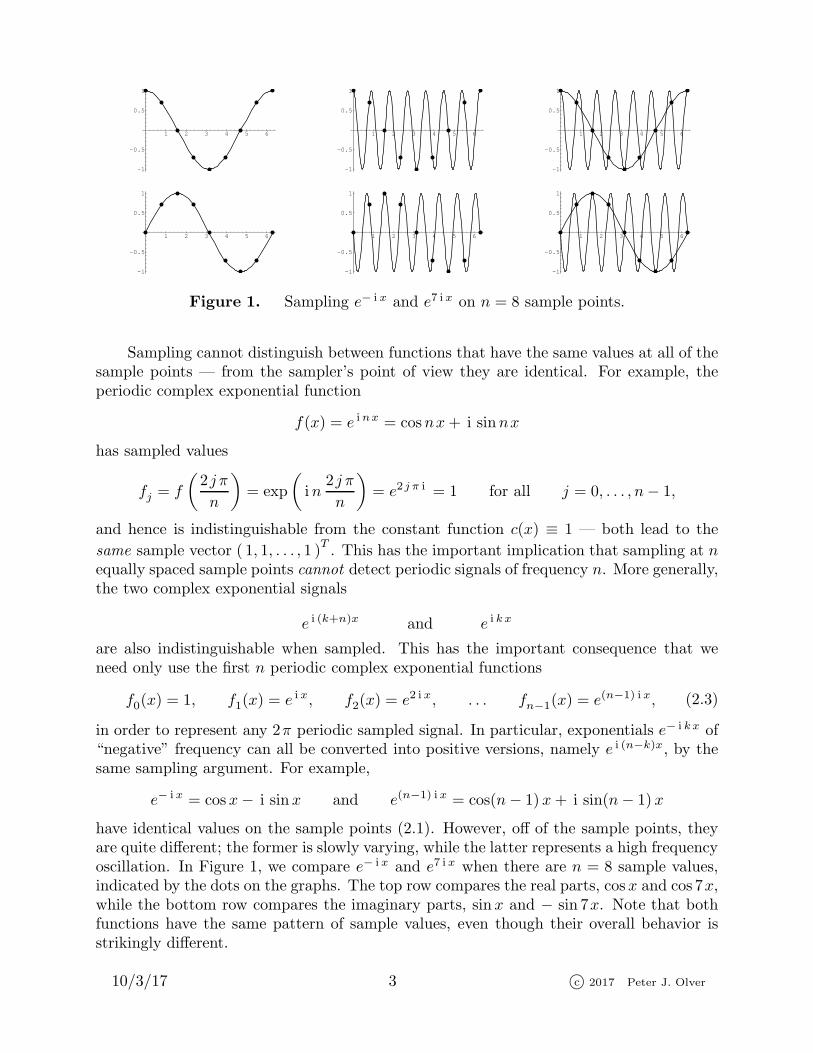
Since it generates all the others, ζn is known as the primitive nth root of unity . Geometri-cally, the nth roots (2.11) lie on the vertices of a regular unit n–gon in the complex plane;

10/3/17 5 c© 2017 Peter J. Olver

ζ05 = 1

ζ5

ζ25

ζ35

ζ45

Figure 2. The Fifth Roots of Unity.

see Figure 2. The primitive root ζn is the first vertex we encounter as we go around then–gon in a counterclockwise direction, starting at 1. Continuing around, the other rootsappear in their natural order ζ2n, ζ

3n, . . . , ζ

n−1n , and finishing back at ζnn = 1. The complex

conjugate of ζn is the “last” nth root

e−2π i /n = ζn =1

ζn= ζn−1

n = e2(n−1)π i /n. (2.12)

The complex numbers (2.11) are a complete set of roots of the polynomial zn − 1,which can therefore be factored:

zn − 1 = (z − 1)(z − ζn)(z − ζ2n) · · · (z − ζn−1n ).

On the other hand, elementary algebra provides us with the real factorization

zn − 1 = (z − 1)(1 + z + z2 + · · · + zn−1).

Comparing the two, we conclude that

1 + z + z2 + · · · + zn−1 = (z − ζn)(z − ζ2n) · · · (z − ζn−1n ).

Substituting z = ζkn into both sides of this identity, we deduce the useful formula

1 + ζkn + ζ2kn + · · · + ζ(n−1)kn =

{n, k = 0,

0, 0 < k < n.(2.13)

Since ζn+kn = ζkn, this formula can easily be extended to general integers k; the sum is

equal to n if n evenly divides k and is 0 otherwise.

Now, let us apply what we’ve learned to prove Proposition 2.1. First, in view of (2.11),the sampled exponential vectors (2.6) can all be written in terms of the nth roots of unity:

ωk =(1, ζkn, ζ

2kn , ζ3kn , . . . , ζ(n−1)k

n

)T, k = 0, . . . , n− 1. (2.14)

Therefore, applying (2.12, 13), we conclude that

〈ωk ;ωl 〉 =1

n

n−1∑

j=0

ζj kn ζjln =1

n

n−1∑

j=0

ζj(k−l)n =

{1, k = l,

0, k 6= l,0 ≤ k, l < n,

10/3/17 6 c© 2017 Peter J. Olver

which establishes orthonormality of the sampled exponential vectors. Q.E.D.

Orthonormality of the basis vectors implies that we can immediately compute theFourier coefficients in the discrete Fourier sum (2.4) by taking inner products:

ck = 〈 f ;ωk 〉 =1

n

n−1∑

j=0

fj e i kxj =1

n

n−1∑

j=0

fj e− i kxj =

1

n

n−1∑

j=0

ζ−j kn fj . (2.15)

In other words, the discrete Fourier coefficient ck is obtained by averaging the sampled val-ues of the product function f(x) e− i kx. The passage from a signal to its Fourier coefficientsis known as the Discrete Fourier Transform or DFT for short. The reverse procedure ofreconstructing a signal from its discrete Fourier coefficients via the sum (2.4) (or (2.7)) isknown as the Inverse Discrete Fourier Transform or IDFT. The Discrete Fourier Transformand its inverse define mutually inverse linear transformations on the space Cn.

Example 2.2. If n = 4, then ζ4 = i . The corresponding sampled exponentialvectors

ω0 =

1111

, ω1 =

1i−1− i

, ω2 =

1−11−1

, ω3 =

1− i−1i

,

form an orthonormal basis of C4 with respect to the averaged Hermitian dot product

〈v ;w 〉 = 14

(v0 w0 + v1 w1 + v2 w2 + v3 w3

), where v =

v0v1v2v3

, w =

w0

w1

w2

w3

.

Given the sampled function values

f0 = f(0), f1 = f(

12π), f2 = f(π), f3 = f

(32π),

we construct the discrete Fourier representation

f = c0 ω0 + c1 ω1 + c2 ω2 + c3 ω3, (2.16)

where

c0 = 〈 f ;ω0 〉 = 14(f0 + f1 + f2 + f3), c1 = 〈 f ;ω1 〉 = 1

4(f0 − i f1 − f2 + i f3),

c2 = 〈 f ;ω2 〉 = 14 (f0 − f1 + f2 − f3), c3 = 〈 f ;ω3 〉 = 1

4 (f0 + i f1 − f2 − i f3).

We interpret this decomposition as the complex exponential interpolant

f(x) ∼ p(x) = c0 + c1 eix + c2 e

2 ix + c3 e3 ix

that agrees with f(x) on the sample points.

For instance, iff(x) = 2πx− x2,

thenf0 = 0., f1 = 7.4022, f2 = 9.8696, f3 = 7.4022,

10/3/17 7 c© 2017 Peter J. Olver

1 2 3 4 5 6

2

4

6

8

10

1 2 3 4 5 6

2

4

6

8

10

1 2 3 4 5 6

2

4

6

8

10

1 2 3 4 5 6

2

4

6

8

10

1 2 3 4 5 6

2

4

6

8

10

1 2 3 4 5 6

2

4

6

8

10

Figure 3. The Discrete Fourier Representation of x2 − 2πx.

and hence

c0 = 6.1685, c1 = −2.4674, c2 = −1.2337, c3 = −2.4674.

Therefore, the interpolating trigonometric polynomial is given by the real part of

p(x) = 6.1685− 2.4674 e ix − 1.2337 e2 ix − 2.4674 e3 ix, (2.17)

namely,

Re p(x) = 6.1685− 2.4674 cosx− 1.2337 cos 2x− 2.4674 cos 3x. (2.18)

In Figure 3 we compare the function, with the interpolation points indicated, and discreteFourier representations (2.18) for both n = 4 and n = 16 points. The resulting graphs pointout a significant difficulty with the Discrete Fourier Transform as developed so far. Whilethe trigonometric polynomials do indeed correctly match the sampled function values, theirpronounced oscillatory behavior makes them completely unsuitable for interpolation awayfrom the sample points.

However, this difficulty can be rectified by being a little more clever. The problem isthat we have not been paying sufficient attention to the frequencies that are represented inthe Fourier sum. Indeed, the graphs in Figure 3 might remind you of our earlier observationthat, due to aliasing, low and high frequency exponentials can have the same sample data,but differ wildly in between the sample points. While the first half of the summands in(2.4) represent relatively low frequencies, the second half do not, and can be replaced byequivalent lower frequency, and hence less oscillatory exponentials. Namely, if 0 < k ≤ 1

2n,

then e− i kx and e i (n−k)x have the same sample values, but the former is of lower frequencythan the latter. Thus, for interpolatory purposes, we should replace the second half of thesummands in the Fourier sum (2.4) by their low frequency alternatives. If n = 2m+ 1 isodd, then we take

p(x) = c−m e− imx+ · · · +c−1 e− i x+c0+c1 e

ix+ · · · +cm e imx =

m∑

k=−m

ck ei kx (2.19)

10/3/17 8 c© 2017 Peter J. Olver

1 2 3 4 5 6

2

4

6

8

10

1 2 3 4 5 6

2

4

6

8

10

1 2 3 4 5 6

2

4

6

8

10

1 2 3 4 5 6

2

4

6

8

10

1 2 3 4 5 6

2

4

6

8

10

1 2 3 4 5 6

2

4

6

8

10

Figure 4. The Low Frequency Discrete Fourier Representation of x2 − 2πx.

as the equivalent low frequency interpolant. If n = 2m is even — which is the mostcommon case occurring in applications — then

p(x) = c−m e− imx+ · · · +c−1 e− ix+c0+c1 e

ix+ · · · +cm−1 ei (m−1)x =

m−1∑

k=−m

ck ei kx

(2.20)will be our choice. (It is a matter of personal taste whether to use e− imx or e imx torepresent the highest frequency term.) In both cases, the Fourier coefficients with negativeindices are the same as their high frequency alternatives:

c−k = cn−k = 〈 f ;ωn−k 〉 = 〈 f ;ω−k 〉, (2.21)

where ω−k = ωn−k is the sample vector for e− i kx ∼ e i (n−k)x.

Returning to the previous example, for interpolating purposes, we should replace(2.17) by the equivalent low frequency interpolant

p (x) = −1.2337 e−2 ix − 2.4674 e− ix + 6.1685− 2.4674 e ix, (2.22)

with real partRe p (x) = 6.1685− 4.9348 cosx− 1.2337 cos 2x.

Graphs of the n = 4 and 16 low frequency trigonometric interpolants can be seen in Fig-ure 4. Thus, by utilizing only the lowest frequency exponentials, we successfully suppressthe aliasing artifacts, resulting in a quite reasonable trigonometric interpolant to the givenfunction.

Remark : The low frequency version also serves to unravel the reality of the Fourierrepresentation of a real function f(x). Since ω−k = ωk, formula (2.21) implies thatc−k = ck, and so the common frequency terms

c−k e− i kx + ck e

i kx = ak cos kx+ bk sin kx

add up to a real trigonometric function. Therefore, the odd n interpolant (2.19) is a realtrigonometric polynomial, whereas in the even version (2.20) only the highest frequencyterm c−m e− imx produces a complex term — which is, in fact, 0 on the sample points.

10/3/17 9 c© 2017 Peter J. Olver

1 2 3 4 5 6

1

2

3

4

5

6

7

The Original Signal

1 2 3 4 5 6

1

2

3

4

5

6

7

The Noisy Signal

1 2 3 4 5 6

1

2

3

4

5

6

7

The Denoised Signal

1 2 3 4 5 6

1

2

3

4

5

6

7

Comparison of the Two

Figure 5. Denoising a Signal.

Compression and Noise Removal

In a typical experimental signal, noise primarily affects the high frequency modes,while the authentic features tend to appear in the low frequencies. Think of the hiss andstatic you hear on an AM radio station or a low quality audio recording. Thus, a verysimple, but effective, method for denoising a corrupted signal is to decompose it into itsFourier modes, as in (2.4), and then discard the high frequency constituents. A similaridea underlies the Dolby©T recording system used on most movie soundtracks: duringthe recording process, the high frequency modes are artificially boosted, so that scalingthem back when showing the movie in the theater has the effect of eliminating much ofthe extraneous noise. The one design issue is the specification of a cut-off between lowand high frequency, that is, between signal and noise. This choice will depend upon theproperties of the measured signal, and is left to the discretion of the signal processor.

A correct implementation of the denoising procedure is facilitated by using the una-liased forms (2.19, 20) of the trigonometric interpolant, in which the low frequency sum-mands only appear when | k | is small. In this version, to eliminate high frequency compo-nents, we replace the full summation by

ql(x) =

l∑

k=− l

ck ei kx, (2.23)

where l < 12 (n + 1) specifies the selected cut-off frequency between signal and noise. The

2 l + 1 ≪ n low frequency Fourier modes retained in (2.23) will, in favorable situations,capture the essential features of the original signal while simultaneously eliminating thehigh frequency noise.

In Figure 5 we display a sample signal followed by the same signal corrupted by addingin random noise. We use n = 29 = 512 sample points in the discrete Fourier representation,

10/3/17 10 c© 2017 Peter J. Olver

1 2 3 4 5 6

1

2

3

4

5

6

7

The Original Signal

1 2 3 4 5 6

1

2

3

4

5

6

7

Moderate Compression

1 2 3 4 5 6

1

2

3

4

5

6

7

High Compression

Figure 6. Compressing a Signal.

and to remove the noise, we retain only the 2 l + 1 = 11 lowest frequency modes. In otherwords, instead of all n = 512 Fourier coefficients c−256, . . . , c−1, c0, c1, . . . , c255, we onlycompute the 11 lowest order ones c−5, . . . , c5. Summing up just those 11 exponentialsproduces the denoised signal q(x) = c−5 e

−5 ix + · · ·+ c5 e5 ix. To compare, we plot both

the original signal and the denoised version on the same graph. In this case, the maximaldeviation is less than .15 over the entire interval [0, 2π ].

The same idea underlies many data compression algorithms for audio recordings, digi-tal images and, particularly, video. The goal is efficient storage and/or transmission of thesignal. As before, we expect all the important features to be contained in the low frequencyconstituents, and so discarding the high frequency terms will, in favorable situations, notlead to any noticeable degradation of the signal or image. Thus, to compress a signal(and, simultaneously, remove high frequency noise), we retain only its low frequency dis-crete Fourier coefficients. The signal is reconstructed by summing the associated truncateddiscrete Fourier series (2.23). A mathematical justification of Fourier-based compressionalgorithms relies on the fact that the Fourier coefficients of smooth functions tend rapidlyto zero — the smoother the function, the faster the decay rate. Thus, the small highfrequency Fourier coefficients will be of negligible importance.

In Figure 6, the same signal is compressed by retaining, respectively, 2 l + 1 = 21and 2 l + 1 = 7 Fourier coefficients only instead of all n = 512 that would be required forcomplete accuracy. For the case of moderate compression, the maximal deviation betweenthe signal and the compressed version is less than 1.5 × 10−4 over the entire interval,while even the highly compressed version deviates at most .05 from the original signal. Ofcourse, the lack of any fine scale features in this particular signal means that a very highcompression can be achieved — the more complicated or detailed the original signal, themore Fourier modes need to be retained for accurate reproduction.

The Fast Fourier Transform

While one may admire an algorithm for its intrinsic beauty, in the real world, thebottom line is always efficiency of implementation: the less total computation, the fasterthe processing, and hence the more extensive the range of applications. Orthogonality isthe first and most important feature of many practical linear algebra algorithms, and is thecritical feature of Fourier analysis. Still, even the power of orthogonality reaches its limitswhen it comes to dealing with truly large scale problems such as three-dimensional medicalimaging or video processing. In the early 1960’s, James Cooley and John Tukey, [4],

10/3/17 11 c© 2017 Peter J. Olver

discovered† a much more efficient approach to the Discrete Fourier Transform, exploitingthe rather special structure of the sampled exponential vectors. The resulting algorithm isknown as the Fast Fourier Transform, often abbreviated FFT, and its discovery launchedthe modern revolution in digital signal and data processing, [2, 3].

In general, computing all the discrete Fourier coefficients (2.15) of an n times sampledsignal requires a total of n2 complex multiplications and n2 − n complex additions. Notealso that each complex addition

z + w = (x+ i y) + (u+ i v) = (x+ u) + i (y + v) (2.24)

generally requires two real additions, while each complex multiplication

zw = (x+ i y)(u+ i v) = (xu− y v) + i (xv + yu) (2.25)

requires 4 real multiplications and 2 real additions, or, by employing the alternative formula

xv + yu = (x+ y)(u+ v)− xu− y v (2.26)

for the imaginary part, 3 real multiplications and 5 real additions. (The choice of formula(2.25) or (2.26) will depend upon the processor’s relative speeds of multiplication and ad-dition.) Similarly, given the Fourier coefficients c0, . . . , cn−1, reconstruction of the sampledsignal via (2.4) requires n2−n complex multiplications and n2−n complex additions. As aresult, both computations become quite labor intensive for large n. Extending these ideasto multi-dimensional data only exacerbates the problem.

In order to explain the method without undue complication, we return to the original,aliased form of the discrete Fourier representation (2.4). (Once one understands how theFFT works, one can easily adapt the algorithm to the low frequency version (2.20).) Theseminal observation is that if the number of sample points

n = 2m

is even, then the primitive mth root of unity ζm = m√1 equals the square of the primitive

nth root:

ζm = ζ2n.

We use this fact to split the summation (2.15) for the order n discrete Fourier coefficients

† In fact, the key ideas can be found in Gauss’ hand computations in the early 1800’s, but hisinsight was not fully appreciated until modern computers arrived on the scene.

10/3/17 12 c© 2017 Peter J. Olver

into two parts, collecting together the even and the odd powers of ζkn:

ck =1

n

(f0 + f1 ζ

−kn + f2 ζ

−2kn + · · · + fn−1 ζ

−(n−1)kn

)

=1

n

(f0 + f2 ζ

−2kn + f4 ζ

−4kn + · · · + f2m−2 ζ

−(2m−2)kn

)+

+ ζ−kn

1

n

(f1 + f3 ζ

−2kn + f5 ζ

−4kn + · · · + f2m−1 ζ

−(2m−2)kn

)

=1

2

{1

m

(f0 + f2 ζ

−km + f4 ζ

−2km + · · · + f2m−2 ζ

−(m−1)km

)}+

+ζ−kn

2

{1

m

(f1 + f3 ζ

−km + f5 ζ

−2km + · · · + f2m−1 ζ

−(m−1)km

)}.

(2.27)

Now, observe that the expressions in braces are the order m Fourier coefficients for thesample data

fe =(f0, f2, f4, . . . , f2m−2

)T=(f(x0), f(x2), f(x4), . . . , f(x2m−2)

)T,

fo =(f1, f3, f5, . . . , f2m−1

)T=(f(x1), f(x3), f(x5), . . . , f(x2m−1)

)T.

(2.28)

Note that fe is obtained by sampling f(x) on the even sample points x2j , while fo isobtained by sampling the same function f(x), but now at the odd sample points x2j+1. Inother words, we are splitting the original sampled signal into two “half-sampled” signalsobtained by sampling on every other point. The even and odd Fourier coefficients are

cek =1

m

(f0 + f2 ζ

−km + f4 ζ

−2km + · · · + f2m−2 ζ

−(m−1)km

),

cok =1

m

(f1 + f3 ζ

−km + f5 ζ

−2km + · · · + f2m−1 ζ

−(m−1)km

),

k = 0, . . . , m−1. (2.29)

Since they contain just m data values, both the even and odd samples require only mdistinct Fourier coefficients, and we adopt the identification

cek+m = cek, cok+m = cok, k = 0, . . . , m− 1. (2.30)

Therefore, the order n = 2m discrete Fourier coefficients (2.27) can be constructed from apair of order m discrete Fourier coefficients via

ck = 12

(cek + ζ−k

n cok), k = 0, . . . , n− 1. (2.31)

Now if m = 2 l is also even, then we can play the same game on the order m Fouriercoefficients (2.29), reconstructing each of them from a pair of order l discrete Fouriercoefficients — obtained by sampling the signal at every fourth point. If n = 2r is a powerof 2, then this game can be played all the way back to the start, beginning with the trivialorder 1 discrete Fourier representation, which just samples the function at a single point.The result is the desired algorithm. After some rearrangement of the basic steps, we arriveat the Fast Fourier Transform, which we now present in its final form.

We begin with a sampled signal on n = 2r sample points. To efficiently programthe Fast Fourier Transform, it helps to write out each index 0 ≤ j < 2r in its binary (as

10/3/17 13 c© 2017 Peter J. Olver

opposed to decimal) representation

j = jr−1 jr−2 . . . j2 j1 j0, where jν = 0 or 1; (2.32)

the notation is shorthand for its r digit binary expansion

j = j0 + 2j1 + 4j2 + 8j3 + · · · + 2r−1 jr−1.

We then define the bit reversal map

ρ(jr−1 jr−2 . . . j2 j1 j0) = j0 j1 j2 . . . jr−2 jr−1. (2.33)

For instance, if r = 5, and j = 13, with 5 digit binary representation 01101, then ρ(j) = 22has the reversed binary representation 10110. Note especially that the bit reversal mapρ = ρr depends upon the original choice of r = log2 n.

Secondly, for each 0 ≤ k < r, define the maps

αk(j) = jr−1 . . . jk+1 0 jk−1 . . . j0,

βk(j) = jr−1 . . . jk+1 1 jk−1 . . . j0 = αk(j) + 2k,for j = jr−1 jr−2 . . . j1 j0.

(2.34)In other words, αk(j) sets the kth binary digit of j to 0, while βk(j) sets it to 1. In thepreceding example, α2(13) = 9, with binary form 01001, while β2(13) = 13 with binaryform 01101. The bit operations (2.33, 34) are especially easy to implement on modernbinary computers.

Given a sampled signal f0, . . . , fn−1, its discrete Fourier coefficients c0, . . . , cn−1 arecomputed by the following iterative algorithm:

c(0)j = fρ(j), c

(k+1)j = 1

2

(c(k)αk(j)

+ ζ−j2k+1 c

(k)βk(j)

),

j = 0, . . . , n− 1,

k = 0, . . . , r − 1,(2.35)

in which ζ2k+1 is the primitive 2k+1 root of unity. The final output of the iterative proce-dure, namely

cj = c(r)j , j = 0, . . . , n− 1, (2.36)

are the discrete Fourier coefficients of our signal. The preprocessing step of the algorithm,

where we define c(0)j , produces a more convenient rearrangement of the sample values. The

subsequent steps successively combine the Fourier coefficients of the appropriate even andodd sampled subsignals together, reproducing (2.27) in a different notation. The followingexample should help make the overall process clearer.

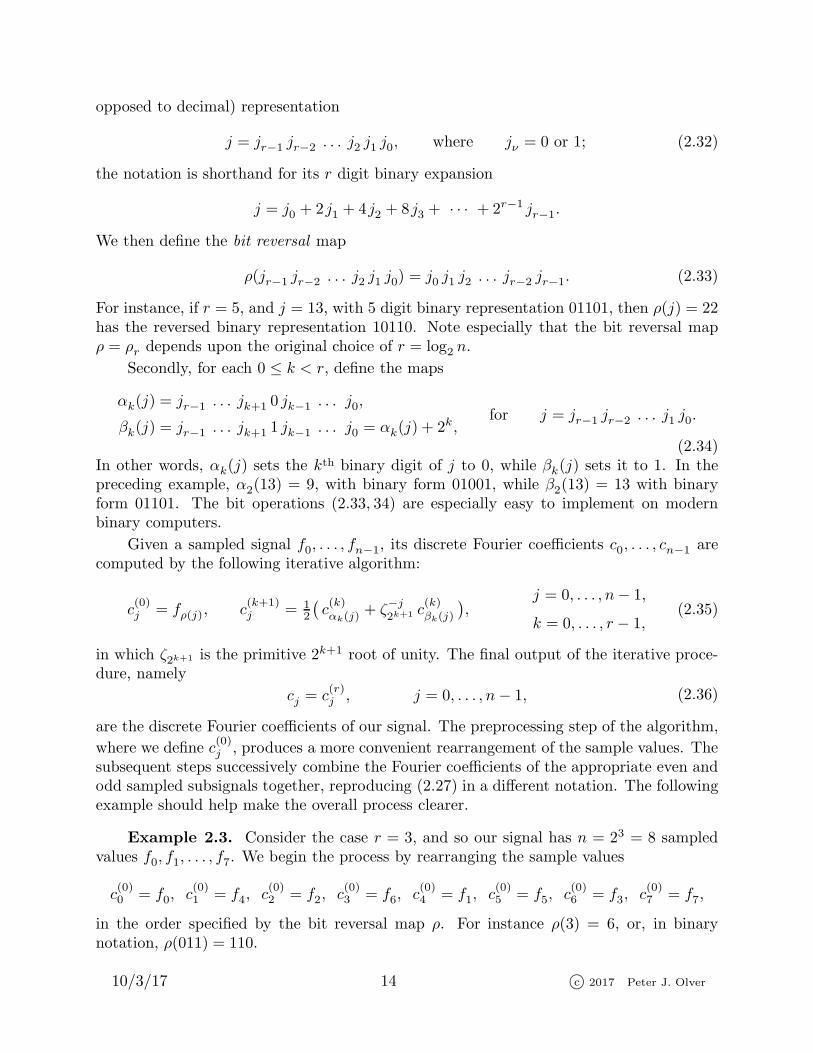
Example 2.3. Consider the case r = 3, and so our signal has n = 23 = 8 sampledvalues f0, f1, . . . , f7. We begin the process by rearranging the sample values

c(0)0 = f0, c

(0)1 = f4, c

(0)2 = f2, c

(0)3 = f6, c

(0)4 = f1, c

(0)5 = f5, c

(0)6 = f3, c

(0)7 = f7,

in the order specified by the bit reversal map ρ. For instance ρ(3) = 6, or, in binarynotation, ρ(011) = 110.

10/3/17 14 c© 2017 Peter J. Olver

The first stage of the iteration is based on ζ2 = −1. Equation (2.35) gives

c(1)0 = 1

2(c

(0)0 + c

(0)1 ), c

(1)1 = 1

2(c

(0)0 − c

(0)1 ), c

(1)2 = 1

2(c

(0)2 + c

(0)3 ), c

(1)3 = 1

2(c

(0)2 − c

(0)3 ),

c(1)4 = 1

2 (c(0)4 + c

(0)5 ), c

(1)5 = 1

2 (c(0)4 − c

(0)5 ), c

(1)6 = 1

2(c(0)6 + c

(0)7 ), c

(1)7 = 1

2 (c(0)6 − c

(0)7 ),

where we combine successive pairs of the rearranged sample values. The second stage ofthe iteration has k = 1 with ζ4 = i . We find

c(2)0 = 1

2 (c(1)0 + c

(1)2 ), c

(2)1 = 1

2 (c(1)1 − i c

(1)3 ), c

(2)2 = 1

2 (c(1)0 − c

(1)2 ), c

(2)3 = 1

2 (c(1)1 + i c

(1)3 ),

c(2)4 = 1

2(c

(1)4 + c

(1)6 ), c

(2)5 = 1

2(c

(1)5 − i c

(1)7 ), c

(2)6 = 1

2(c

(1)4 − c

(1)6 ), c

(2)7 = 1

2(c

(1)5 + i c

(1)7 ).

Note that the indices of the combined pairs of coefficients differ by 2. In the last step,

where k = 2 and ζ8 =√22

(1 + i ), we combine coefficients whose indices differ by 4 = 22;the final output

c0 = c(3)0 = 1

2 (c(2)0 + c

(2)4 ), c4 = c

(3)4 = 1

2(c(2)0 − c

(2)4 ),

c1 = c(3)1 = 1

2

(c(2)1 +

√22

(1− i ) c(2)5

), c5 = c

(3)5 = 1

2

(c(2)1 −

√22

(1− i ) c(2)5

),

c2 = c(3)2 = 1

2

(c(2)2 − i c

(2)6

), c6 = c

(3)6 = 1

2

(c(2)2 + i c

(2)6

),

c3 = c(3)3 = 1

2

(c(2)3 −

√22 (1 + i ) c

(2)7

), c7 = c

(3)7 = 1

2

(c(2)3 +

√22 (1 + i ) c

(2)7

),

is the complete set of discrete Fourier coefficients.

Let us count the number of arithmetic operations required in the Fast Fourier Trans-form algorithm. At each stage in the computation, we must perform n = 2r complexadditions/subtractions and the same number of complex multiplications. (Actually, thenumber of multiplications is slightly smaller since multiplications by ±1 and ± i are ex-tremely simple. However, this does not significantly alter the final operations count.)There are r = log2 n stages, and so we require a total of r n = n log2 n complex addi-tions/subtractions and the same number of multiplications. Now, when n is large, n log2 nis significantly smaller than n2, which is the number of operations required for the directalgorithm. For instance, if n = 210 = 1, 024, then n2 = 1, 048, 576, while n log2 n = 10, 240— a net savings of 99%. As a result, many large scale computations that would be in-tractable using the direct approach are immediately brought into the realm of feasibility.This is the reason why all modern implementations of the Discrete Fourier Transform arebased on the FFT algorithm and its variants.

The reconstruction of the signal from the discrete Fourier coefficients c0, . . . , cn−1 is

speeded up in exactly the same manner. The only differences are that we replace ζ−1n = ζn

by ζn, and drop the factors of 12 since there is no need to divide by n in the final result

(2.4). Therefore, we apply the slightly modified iterative procedure

f(0)j = cρ(j), f

(k+1)j = f

(k)αk(j)

+ ζj2k+1 f

(k)βk(j)

,j = 0, . . . , n− 1,

k = 0, . . . , r − 1,(2.37)

and finish with

f(xj) = fj = f(r)j , j = 0, . . . , n− 1. (2.38)

10/3/17 15 c© 2017 Peter J. Olver

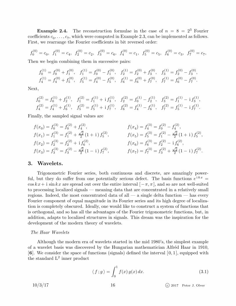
Example 2.4. The reconstruction formulae in the case of n = 8 = 23 Fouriercoefficients c0, . . . , c7, which were computed in Example 2.3, can be implemented as follows.First, we rearrange the Fourier coefficients in bit reversed order:

f(0)0 = c0, f

(0)1 = c4, f

(0)2 = c2, f

(0)3 = c6, f

(0)4 = c1, f

(0)5 = c5, f

(0)6 = c3, f

(0)7 = c7,

Then we begin combining them in successive pairs:

f(1)0 = f

(0)0 + f

(0)1 , f

(1)1 = f

(0)0 − f

(0)1 , f

(1)2 = f

(0)2 + f

(0)3 , f

(1)3 = f

(0)2 − f

(0)3 ,

f(1)4 = f

(0)4 + f

(0)5 , f

(1)5 = f

(0)4 − f

(0)5 , f

(1)6 = f

(0)6 + f

(0)7 , f

(1)7 = f

(0)6 − f

(0)7 .

Next,

f(2)0 = f

(1)0 + f

(1)2 , f

(2)1 = f

(1)1 + i f

(1)3 , f

(2)2 = f

(1)0 − f

(1)2 , f

(2)3 = f

(1)1 − i f

(1)3 ,

f(2)4 = f

(1)4 + f

(1)6 , f

(2)5 = f

(1)5 + i f

(1)7 , f

(2)6 = f

(1)4 − f

(1)6 , f

(2)7 = f

(1)5 − i f

(1)7 .

Finally, the sampled signal values are

f(x0) = f(3)0 = f

(2)0 + f

(2)4 , f(x4) = f

(3)4 = f

(2)0 − f

(2)4 ,

f(x1) = f(3)1 = f

(2)1 +

√22 (1 + i ) f

(2)5 , f(x5) = f

(3)5 = f

(2)1 −

√22 (1 + i ) f

(2)5 ,

f(x2) = f(3)2 = f

(2)2 + i f

(2)6 , f(x6) = f

(3)6 = f

(2)2 − i f

(2)6 ,

f(x3) = f(3)3 = f

(2)3 −

√22 (1− i ) f

(2)7 , f(x7) = f

(3)7 = f

(2)3 +

√22 (1− i ) f

(2)7 .

3. Wavelets.

Trigonometric Fourier series, both continuous and discrete, are amazingly power-ful, but they do suffer from one potentially serious defect. The basis functions e i kx =cos kx+ i sin kx are spread out over the entire interval [−π, π ], and so are not well-suitedto processing localized signals — meaning data that are concentrated in a relatively smallregions. Indeed, the most concentrated data of all — a single delta function — has everyFourier component of equal magnitude in its Fourier series and its high degree of localiza-tion is completely obscured. Ideally, one would like to construct a system of functions thatis orthogonal, and so has all the advantages of the Fourier trigonometric functions, but, inaddition, adapts to localized structures in signals. This dream was the inspiration for thedevelopment of the modern theory of wavelets.

The Haar Wavelets

Although the modern era of wavelets started in the mid 1980’s, the simplest exampleof a wavelet basis was discovered by the Hungarian mathematician Alfred Haar in 1910,[6]. We consider the space of functions (signals) defined the interval [0, 1], equipped withthe standard L2 inner product

〈 f ; g 〉 =∫ 1

0

f(x) g(x)dx. (3.1)

10/3/17 16 c© 2017 Peter J. Olver

-0.2 0.2 0.4 0.6 0.8 1 1.2

-1

-0.5

0.5

1

ϕ1(x)

-0.2 0.2 0.4 0.6 0.8 1 1.2

-1

-0.5

0.5

1

ϕ2(x)

-0.2 0.2 0.4 0.6 0.8 1 1.2

-1

-0.5

0.5

1

ϕ3(x)

-0.2 0.2 0.4 0.6 0.8 1 1.2

-1

-0.5

0.5

1

ϕ4(x)

Figure 7. The First Four Haar Wavelets.

This choice is merely for convenience, being slightly better suited to our construction than[−π, π ] or [0, 2π ]. Moreover, the usual scaling arguments can be used to adapt the waveletformulas to any other interval.

The Haar wavelets are certain piecewise constant functions. The first four are graphedin Figure 7 The first is the box function

ϕ1(x) = ϕ(x) =

{1, 0 < x ≤ 1,

0, otherwise,(3.2)

known as the scaling function, for reasons that shall appear shortly. Although we are onlyinterested in the value of ϕ(x) on the interval [0, 1], it will be convenient to extend it, andall the other wavelets, to be zero outside the basic interval. Its values at the points ofdiscontinuity, i.e., 0, 1, is not critical, but, unlike the Fourier series midpoint value, it willbe more convenient to consistently choose the left hand limiting value. The second Haarfunction

ϕ2(x) = w(x) =

1, 0 < x ≤ 12 ,

−1, 12< x ≤ 1,

0, otherwise,

(3.3)

is known as the mother wavelet . The third and fourth Haar functions are compressed

10/3/17 17 c© 2017 Peter J. Olver

versions of the mother wavelet:

ϕ3(x) = w(2x) =

1, 0 < x ≤ 14 ,

−1, 14 < x ≤ 1

2 ,

0, otherwise,

ϕ4(x) = w(2x− 1) =

1, 12 < x ≤ 3

4 ,

−1, 34 < x ≤ 1,

0, otherwise,

called daughter wavelets . One can easily check, by direct evaluation of the integrals, thatthe four Haar wavelet functions are orthogonal with respect to the L2 inner product (3.1).

The scaling transformation x 7→ 2x serves to compress the wavelet function, whilethe translation 2x 7→ 2x − 1 moves the compressed version to the right by a half a unit.Furthermore, we can represent the mother wavelet by compressing and translating thescaling function,:

w(x) = ϕ(2x)− ϕ(2x− 1). (3.4)

It is these two operations of scaling and compression — coupled with the all-importantorthogonality — that underlies the power of wavelets.

The Haar wavelets have an evident discretization. If we decompose the interval (0, 1]into the four subintervals

(0 , 1

4

],

(14, 12

],

(12, 34

],

(34, 1], (3.5)

on which the four wavelet functions are constant, then we can represent each of them bya vector in R4 whose entries are the values of each wavelet function sampled at the leftendpoint of each subinterval. In this manner, we obtain the wavelet sample vectors

v1 =

1111

, v2 =

11−1−1

, v3 =

1−100

, v4 =

001−1

. (3.6)

Orthogonality of the vectors (3.6) with respect to the standard Euclidean dot product isequivalent to orthogonality of the Haar wavelet functions with respect to the inner product(3.1). Indeed, if

f(x) ∼ f = (f1, f2, f3, f4) and g(x) ∼ g = (g1, g2, g3, g4)

are piecewise constant real functions that achieve the indicated values on the four subin-tervals (3.5), then their L2 inner product

〈 f ; g 〉 =∫ 1

0

f(x) g(x)dx = 14

(f1 g1 + f2 g2 + f3 g3 + f4 g4

)= 1

4 f · g,

is equal to the averaged dot product of their sample values — the real form of the innerproduct (2.8) that was used in the discrete Fourier transform.

Since the vectors (3.6) form an orthogonal basis of R4, we can uniquely decomposeany such piecewise constant function as a linear combination of wavelets

f(x) = c1ϕ1(x) + c2ϕ2(x) + c3ϕ3(x) + c4ϕ4(x),

10/3/17 18 c© 2017 Peter J. Olver

or, equivalently, in terms of the sample vectors,

f = c1v1 + c2v2 + c3v3 + c4v4.

The required coefficients

ck =〈 f ;ϕk 〉‖ϕk ‖2

=f · vk

‖vk ‖2

are fixed by our usual orthogonality. Explicitly,

c1 = 14(f1 + f2 + f3 + f4),

c2 = 14 (f1 + f2 − f3 − f4),

c3 = 12(f1 − f2),

c4 = 12 (f3 − f4).

Before proceeding to the more general case, let us introduce an important analyticaldefinition that quantifies precisely how localized a function is.

Definition 3.1. The support of a function f(x), written supp f , is the closure of theset where f(x) 6= 0.

Thus, a point will belong to the support of f(x), provided f is not zero there, or atleast is not zero at nearby points. More precisely:

Lemma 3.2. If f(a) 6= 0, then a ∈ supp f . More generally, a point a ∈ supp f if

and only if there exist a convergent sequence xn → a such that f(xn) 6= 0. Conversely,

a 6∈ supp f if and only if f(x) ≡ 0 on an interval a− δ < x < a+ δ for some δ > 0.

Intuitively, the smaller the support of a function, the more localized it is. For example,the support of the Haar mother wavelet (3.3) is suppw = [0, 1] — the point x = 0 isincluded, even though w(0) = 0, because w(x) 6= 0 at nearby points. The two daughterwavelets have smaller support:

suppϕ3 =[0 , 1

2

], suppϕ4 =

[12, 1],

and so are twice as localized. An extreme case is the delta function, whose support is asingle point. In contrast, the support of the Fourier trigonometric basis functions is all ofR, since they only vanish at isolated points.

The effect of scalings and translations on the support of a function is easily discerned.

Lemma 3.3. If supp f = [a, b ], and

g(x) = f(rx− δ), then supp g =

[a+ δ

r,b+ δ

r

].

In other words, scaling x by a factor r compresses the support of the function by afactor 1/r, while translating x translates the support of the function.

The key requirement for a wavelet basis is that it contains functions with arbitrarilysmall support. To this end, the full Haar wavelet basis is obtained from the mother waveletby iterating the scaling and translation processes. We begin with the scaling function

ϕ(x), (3.7)

10/3/17 19 c© 2017 Peter J. Olver

from which we construct the mother wavelet via (3.4). For any “generation” j ≥ 0, weform the wavelet offspring by first compressing the mother wavelet so that its support fitsinto an interval of length 2−j ,

wj,0(x) = w(2j x), so that suppwj,0 = [0, 2−j ], (3.8)

and then translating wj,0 so as to fill up the entire interval [0, 1] by 2j subintervals, each

of length 2−j , defining

wj,k(x) = wj,0(x− k) = w(2j x− k), where k = 0, 1, . . .2j − 1. (3.9)

Lemma 3.3 implies that suppwj,k = [ 2−j k, 2−j (k+1) ], and so the combined supports of

all the jth generation of wavelets is the entire interval:2j−1⋃

k=0

suppwj,k = [0, 1] . The primal

generation, j = 0, just consists of the mother wavelet

w0,0(x) = w(x).

The first generation, j = 1, consists of the two daughter wavelets already introduced asϕ3 and ϕ4, namely

w1,0(x) = w(2x), w1,1(x) = w(2x− 1).

The second generation, j = 2, appends four additional granddaughter wavelets to ourbasis:

w2,0(x) = w(4x), w2,1(x) = w(4x− 1), w2,2(x) = w(4x− 2), w2,3(x) = w(4x− 3).

The 8 Haar wavelets ϕ,w0,0, w1,0, w1,1, w2,0, w2,1, w2,2, w2,3 are constant on the 8 subin-

tervals of length 18 , taking the successive sample values indicated by the columns of the

matrix

W8 =

1 1 1 0 1 0 0 01 1 1 0 −1 0 0 01 1 −1 0 0 1 0 01 1 −1 0 0 −1 0 01 −1 0 1 0 0 1 01 −1 0 1 0 0 −1 01 −1 0 −1 0 0 0 11 −1 0 −1 0 0 0 −1

. (3.10)

Orthogonality of the wavelets is manifested in the orthogonality of the columns of W8.(Unfortunately, terminological constraints prevent us from callingW8 an orthogonal matrixbecause its columns are not orthonormal!)

The nth stage consists of 2n+1 different wavelet functions comprising the scaling func-tions and all the generations up to the nth : w0(x) = ϕ(x) and wj,k(x) for 0 ≤ j ≤ n and

0 ≤ k < 2j . They are all constant on each subinterval of length 2−n−1.

Theorem 3.4. The wavelet functions ϕ(x), wj,k(x) form an orthogonal system with

respect to the inner product (3.1).

10/3/17 20 c© 2017 Peter J. Olver

Proof : First, note that each wavelet wj,k(x) is equal to +1 on an interval of length

2−j−1 and to −1 on an adjacent interval of the same length. Therefore,

〈wj,k ;ϕ 〉 =∫ 1

0

wj,k(x) dx = 0, (3.11)

since the +1 and −1 contributions cancel each other. If two different wavelets wj,k andwl,m with, say j ≤ l, have supports which are either disjoint, or just overlap at a singlepoint, then their product wj,k(x)wl,m(x) ≡ 0, and so their inner product is clearly zero:

〈wj,k ;wl,m 〉 =∫ 1

0

wj,k(x)wl,m(x) dx = 0.

Otherwise, except in the case when the two wavelets are identical, the support of wl,m isentirely contained in an interval where wj,k is constant and so wj,k(x)wl,m(x) = ±wl,m(x).Therefore, by (3.11),

〈wj,k ;wl,m 〉 =∫ 1

0

wj,k(x)wl,m(x) dx = ±∫ 1

0

wl,m(x) dx = 0.

Finally, we compute

‖ϕ ‖2 =

∫ 1

0

dx = 1, ‖wj,k ‖2 =

∫ 1

0

wj,k(x)2 dx = 2−j . (3.12)

The second formula follows from the fact that |wj,k(x) | = 1 on an interval of length 2−j

and is 0 elsewhere. Q.E.D.

In direct analogy with the trigonometric Fourier series, the wavelet series of a signalf(x) is given by

f(x) ∼ c0 ϕ(x) +∞∑

j=0

2j−1∑

k=0

cj,k wj,k(x). (3.13)

Orthogonality implies that the wavelet coefficients c0, cj,k can be immediately computedusing the standard inner product formula coupled with (3.12):

c0 =〈 f ;ϕ 〉‖ϕ ‖2 =

∫ 1

0

f(x)dx,

cj,k =〈 f ;wj,k 〉‖wj,k ‖2

= 2j∫ 2−jk+2−j−1

2−jk

f(x)dx − 2j∫ 2−j(k+1)

2−jk+2−j−1

f(x)dx.

(3.14)

The convergence properties of the wavelet series (3.13) are similar to those of Fourier series;details can be found [5].

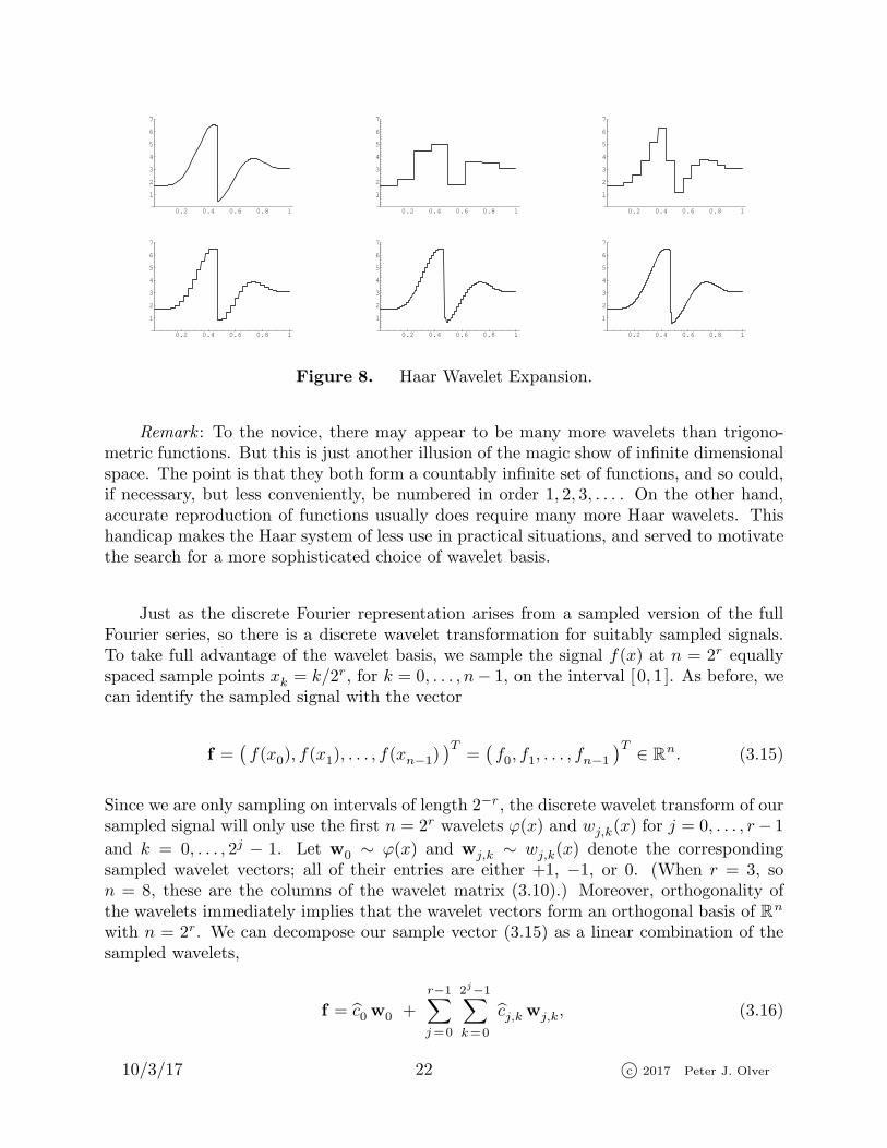
Example 3.5. In Figure 8, we plot the Haar expansions of the signal in the first plot.The next plots show the partial sums over j = 0, . . . , r with r = 2, 3, 4, 5, 6. We have useda discontinuous signal to demonstrate that there is no nonuniform Gibbs phenomenon ina Haar wavelet expansion. Indeed, since the wavelets are themselves discontinuous, theydo not have any difficult uniformly converging to a discontinuous function. On the otherhand, it takes quite a few wavelets to begin to accurately reproduce the signal. In the lastplot, we combine a total of 26 = 64 Haar wavelets, which is considerably more than wouldbe required in a comparably accurate Fourier expansion (excluding points very close tothe discontinuity).

10/3/17 21 c© 2017 Peter J. Olver

0.2 0.4 0.6 0.8 1

1

2

3

4

5

6

7

0.2 0.4 0.6 0.8 1

1

2

3

4

5

6

7

0.2 0.4 0.6 0.8 1

1

2

3

4

5

6

7

0.2 0.4 0.6 0.8 1

1

2

3

4

5

6

7

0.2 0.4 0.6 0.8 1

1

2

3

4

5

6

7

0.2 0.4 0.6 0.8 1

1

2

3

4

5

6

7

Figure 8. Haar Wavelet Expansion.

Remark : To the novice, there may appear to be many more wavelets than trigono-metric functions. But this is just another illusion of the magic show of infinite dimensionalspace. The point is that they both form a countably infinite set of functions, and so could,if necessary, but less conveniently, be numbered in order 1, 2, 3, . . . . On the other hand,accurate reproduction of functions usually does require many more Haar wavelets. Thishandicap makes the Haar system of less use in practical situations, and served to motivatethe search for a more sophisticated choice of wavelet basis.

Just as the discrete Fourier representation arises from a sampled version of the fullFourier series, so there is a discrete wavelet transformation for suitably sampled signals.To take full advantage of the wavelet basis, we sample the signal f(x) at n = 2r equallyspaced sample points xk = k/2r, for k = 0, . . . , n− 1, on the interval [0, 1]. As before, wecan identify the sampled signal with the vector

f =(f(x0), f(x1), . . . , f(xn−1)

)T=(f0, f1, . . . , fn−1

)T ∈ Rn. (3.15)

Since we are only sampling on intervals of length 2−r, the discrete wavelet transform of oursampled signal will only use the first n = 2r wavelets ϕ(x) and wj,k(x) for j = 0, . . . , r− 1

and k = 0, . . . , 2j − 1. Let w0 ∼ ϕ(x) and wj,k ∼ wj,k(x) denote the correspondingsampled wavelet vectors; all of their entries are either +1, −1, or 0. (When r = 3, son = 8, these are the columns of the wavelet matrix (3.10).) Moreover, orthogonality ofthe wavelets immediately implies that the wavelet vectors form an orthogonal basis of Rn

with n = 2r. We can decompose our sample vector (3.15) as a linear combination of thesampled wavelets,

f = c0 w0 +

r−1∑

j=0

2j−1∑

k=0

cj,k wj,k, (3.16)

10/3/17 22 c© 2017 Peter J. Olver

where, by our usual orthogonality formulae,

c0 =〈 f ;w0 〉‖w0 ‖2

=1

2r

2r−1∑

i=0

fi,

cj,k =〈 f ;wj,k 〉‖wj,k ‖2

= 2j−r

k+2r−j−1−1∑

i=k

fi −k+2r−j−1∑

i=k+2r−j−1

fi

.

(3.17)

These are the basic formulae connecting the functions f(x), or, rather, its sample vectorf , and its discrete wavelet transform consisting of the 2r coefficients c0, cj,k. The recon-structed function

f(x) = c0 ϕ(x) +

r−1∑

j=0

2j−1∑

k=0

cj,k wj,k(x) (3.18)

is constant on each subinterval of length 2−r, and has the same value

f(x) = f(xi) = f(xi) = fi, xi = 2−r i ≤ x < xi+1 = 2−r (i+ 1),

as our signal at the left hand endpoint of the interval. In other words, we are interpolatingthe sample points by a piecewise constant (and thus discontinuous) function.

Modern Wavelets

The main defect of the Haar wavelets is that they do not provide a very efficient meansof representing even very simple functions — it takes quite a large number of wavelets toreproduce signals with any degree of precision. The reason for this is that the Haarwavelets are piecewise constant, and so even an affine function y = αx+ β requires manysample values, and hence a relatively extensive collection of Haar wavelets, to be accuratelyreproduced. In particular, compression and denoising algorithms based on Haar waveletsare either insufficiently precise or hopelessly inefficient, and hence of minor practical value.

For a long time it was thought that it was impossible to simultaneously achieve therequirements of localization, orthogonality and accurate reproduction of simple functions.The breakthrough came in 1988, when, in her Ph.D. thesis, the Dutch mathematician In-grid Daubechies produced the first examples of wavelet bases that realized all three basiccriteria. Since then, wavelets have developed into a sophisticated and burgeoning industrywith major impact on modern technology. Significant applications include compression,storage and recognition of fingerprints in the FBI’s data base, and the JPEG2000 imageformat, which, unlike earlier Fourier-based JPEG standards, incorporates wavelet tech-nology in its image compression and reconstruction algorithms. In this section, we willpresent a brief outline of the basic ideas underlying Daubechies’ remarkable construction.

The recipe for any wavelet system involves two basic ingredients — a scaling functionand a mother wavelet. The latter can be constructed from the scaling function by aprescription similar to that in (3.4), and therefore we first concentrate on the properties ofthe scaling function. The key requirement is that the scaling function must solve a dilation

10/3/17 23 c© 2017 Peter J. Olver

-2 -1 1 2 3 4-0.2

0.2

0.4

0.6

0.8

1

1.2

Figure 9. The Hat Function.

equation of the form

ϕ(x) =

p∑

k=0

ck ϕ(2x− k) = c0 ϕ(2x) + c1 ϕ(2x− 1) + · · · + cp ϕ(2x− p) (3.19)

for some collection of constants c0, . . . , cp. The dilation equation relates the function ϕ(x)to a finite linear combination of its compressed translates. The coefficients c0, . . . , cp arenot arbitrary, since the properties of orthogonality and localization will impose certainrather stringent requirements.

Example 3.6. The Haar or box scaling function (3.2) satisfies the dilation equation(3.19) with c0 = c1 = 1, namely

ϕ(x) = ϕ(2x) + ϕ(2x− 1). (3.20)

We recommend that you convince yourself of the validity of this identity before continuing.

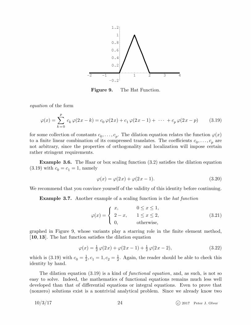
Example 3.7. Another example of a scaling function is the hat function

ϕ(x) =

x, 0 ≤ x ≤ 1,

2− x, 1 ≤ x ≤ 2,

0, otherwise,

(3.21)

graphed in Figure 9, whose variants play a starring role in the finite element method,[10, 13]. The hat function satisfies the dilation equation

ϕ(x) = 12 ϕ(2x) + ϕ(2x− 1) + 1

2 ϕ(2x− 2), (3.22)

which is (3.19) with c0 = 12, c1 = 1, c2 = 1

2. Again, the reader should be able to check this

identity by hand.

The dilation equation (3.19) is a kind of functional equation, and, as such, is not soeasy to solve. Indeed, the mathematics of functional equations remains much less welldeveloped than that of differential equations or integral equations. Even to prove that(nonzero) solutions exist is a nontrivial analytical problem. Since we already know two

10/3/17 24 c© 2017 Peter J. Olver

explicit examples, let us defer the discussion of solution techniques until we understandhow the dilation equation can be used to construct a wavelet basis.

Given a solution to the dilation equation, we define the mother wavelet to be

w(x) =

p∑

k=0

(−1)kcp−k ϕ(2x− k)

= cp ϕ(2x)− cp−1 ϕ(2x− 1) + cp−2 ϕ(2x− 2) + · · · ± c0 ϕ(2x− p),

(3.23)

This formula directly generalizes the Haar wavelet relation (3.4), in light of its dilationequation (3.20). The daughter wavelets are then all found, as in the Haar basis, by itera-tively compressing and translating the mother wavelet:

wj,k(x) = w(2j x− k). (3.24)

In the general framework, we do not necessarily restrict our attention to the interval [0, 1]and so j and k can, in principle, be arbitrary integers.

Let us investigate what sort of conditions should be imposed on the dilation coeffi-cients c0, . . . , cp in order that we obtain a viable wavelet basis by this construction. First,localization of the wavelets requires that the scaling function has bounded support, andso ϕ(x) ≡ 0 when x lies outside some bounded interval [a, b ]. If we integrate both sides of(3.19), we find

∫ b

a

ϕ(x) dx =

∫ ∞

−∞ϕ(x) dx =

p∑

k=0

ck

∫ ∞

−∞ϕ(2x− k) dx. (3.25)

Now using the change of variables y = 2x− k, with dx = 12 dy, we find

∫ ∞

−∞ϕ(2x− k) dx =

1

2

∫ ∞

−∞ϕ(y) dy =

1

2

∫ b

a

ϕ(x) dx, (3.26)

where we revert to x as our (dummy) integration variable. We substitute this result back

into (3.25). Assuming that

∫ b

a

ϕ(x) dx 6= 0, we discover that the dilation coefficients must

satisfy

c0 + · · · + cp = 2. (3.27)

Example 3.8. Once we impose the constraint (3.27), the very simplest version ofthe dilation equation is

ϕ(x) = 2ϕ(2x) (3.28)

where c0 = 2 is the only (nonzero) coefficient. Up to constant multiple, the only “solutions”of the functional equation (3.28) with bounded support are scalar multiples of the deltafunction δ(x). Other solutions, such as ϕ(x) = 1/x, are not localized, and thus not usefulfor constructing a wavelet basis.

10/3/17 25 c© 2017 Peter J. Olver

The second condition we require is orthogonality of the wavelets. For simplicity, weonly consider the standard L2 inner product†

〈 f ; g 〉 =∫ ∞

−∞f(x) g(x)dx.

It turns out that the orthogonality of the complete wavelet system is guaranteed once weknow that the scaling function ϕ(x) is orthogonal to all its integer translates:

〈ϕ(x) ;ϕ(x−m) 〉 =∫ ∞

−∞ϕ(x)ϕ(x−m) dx = 0 for all m 6= 0. (3.29)

We first note the formula

〈ϕ(2x− k) ;ϕ(2x− l) 〉 =∫ ∞

−∞ϕ(2x− k)ϕ(2x− l) dx (3.30)

=1

2

∫ ∞

−∞ϕ(x)ϕ(x+ k − l) dx =

1

2〈ϕ(x) ;ϕ(x+ k − l) 〉

follows from the same change of variables y = 2x − k used in (3.26). Therefore, since ϕsatisfies the dilation equation (3.19),

〈ϕ(x) ;ϕ(x−m) 〉 =⟨

p∑

j=0

cj ϕ(2x− j) ;

p∑

k=0

ck ϕ(2x− 2m− k)

⟩(3.31)

=

p∑

j,k=0

cj ck 〈ϕ(2x− j) ;ϕ(2x− 2m− k) 〉 = 1

2

p∑

j,k=0

cj ck 〈ϕ(x) ;ϕ(x+ j − 2m− k) 〉.

If we require orthogonality (3.29) of all the integer translates of ϕ, then the left hand sideof this identity will be 0 unless m = 0, while only the summands with j = 2m+ k will benonzero on the right. Therefore, orthogonality requires that

∑

0 ≤ k ≤ p−2m

c2m+k ck =

{2, m = 0,

0, m 6= 0.(3.32)

The algebraic equations (3.27, 32) for the dilation coefficients are the key requirements forthe construction of an orthogonal wavelet basis.

For example, if we have just two nonzero coefficients c0, c1, then (3.27, 32) reduce to

c0 + c1 = 2, c20 + c21 = 2,

and so c0 = c1 = 1 is the only solution, resulting in the Haar dilation equation (3.20). Ifwe have three coefficients c0, c1, c2, then (3.27), (3.32) require

c0 + c1 + c2 = 2, c20 + c21 + c22 = 2, c0 c2 = 0.

† In all instances, the functions have bounded support, and so the inner product integral canbe reduced to an integral over a finite interval where both f and g are nonzero.

10/3/17 26 c© 2017 Peter J. Olver

Thus either c2 = 0, c0 = c1 = 1, and we are back to the Haar case, or c0 = 0, c1 = c2 = 1,and the resulting dilation equation is a simple reformulation of the Haar case. In particular,the hat function (3.21) does not give rise to orthogonal wavelets.

The remarkable fact, discovered by Daubechies, is that there is a nontrivial solutionfor four (and, indeed, any even number) of nonzero coefficients c0, c1, c2, c3. The basicequations (3.27), (3.32) require

c0 + c1 + c2 + c3 = 2, c20 + c21 + c22 + c23 = 2, c0 c2 + c1 c3 = 0. (3.33)

The particular values

c0 = 1+√3

4, c1 = 3+

√3

4, c2 = 3−

√3

4, c3 = 1−

√3

4, (3.34)

solve (3.33). These coefficients correspond to the Daubechies dilation equation

ϕ(x) = 1+√3

4 ϕ(2x) + 3+√3

4 ϕ(2x− 1) + 3−√3

4 ϕ(2x− 2) + 1−√3

4 ϕ(2x− 3). (3.35)

Any nonzero solution of bounded support to this remarkable functional equation will giverise to a scaling function ϕ(x), a mother wavelet

w(x) = 1−√3

4ϕ(2x)− 3−

√3

4ϕ(2x− 1) + 3+

√3

4ϕ(2x− 2)− 1+

√3

4ϕ(2x− 3), (3.36)

and then, by compression and translation (3.24), the complete system of orthogonalwavelets wj,k(x).

Before explaining how to solve the Daubechies dilation equation, let us complete theproof of orthogonality. It is easy to see that, by translation invariance, since ϕ(x) andϕ(x−m) are orthogonal for any m 6= 0, so are ϕ(x− k) and ϕ(x− l) for any k 6= l. Nextwe prove orthogonality of ϕ(x−m) and w(x):

〈w(x) ;ϕ(x−m) 〉 =⟨

p∑

j=0

(−1)j+1 cj ϕ(2x− 1 + j) ;

p∑

k=0

ck ϕ(2x− 2m− k)

⟩

=

p∑

j,k=0

(−1)j+1 cj ck 〈ϕ(2x− 1 + j) ;ϕ(2x− 2m− k) 〉

=1

2

p∑

j,k=0

(−1)j+1 cj ck 〈ϕ(x) ;ϕ(x− 1 + j − 2m− k) 〉,

using (3.30). By orthogonality (3.29) of the translates of ϕ, the only summands that arenonzero are when j = 2m+ k + 1; the resulting coefficient of ‖ϕ(x) ‖2 is

∑

k

(−1)k c1−2m−k ck = 0,

where the sum is over all 0 ≤ k ≤ p such that 0 ≤ 1− 2m− k ≤ p. Each term in the sumappears twice, with opposite signs, and hence the result is always zero — no matter whatthe coefficients c0, . . . , cp are! The proof of orthogonality of the translates w(x − m) of

the mother wavelet, along with all her wavelet descendants w(2j x− k), relies on a similarargument, and the details are left as an exercise for the reader.

10/3/17 27 c© 2017 Peter J. Olver

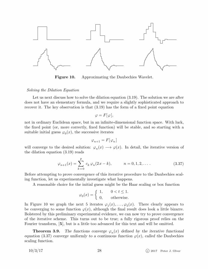
Figure 10. Approximating the Daubechies Wavelet.

Solving the Dilation Equation

Let us next discuss how to solve the dilation equation (3.19). The solution we are afterdoes not have an elementary formula, and we require a slightly sophisticated approach torecover it. The key observation is that (3.19) has the form of a fixed point equation

ϕ = F [ϕ ],

not in ordinary Euclidean space, but in an infinite-dimensional function space. With luck,the fixed point (or, more correctly, fixed function) will be stable, and so starting with asuitable initial guess ϕ0(x), the successive iterates

ϕn+1 = F [ϕn ]

will converge to the desired solution: ϕn(x) −→ ϕ(x). In detail, the iterative version ofthe dilation equation (3.19) reads

ϕn+1(x) =

p∑

k=0

ck ϕn(2x− k), n = 0, 1, 2, . . . . (3.37)

Before attempting to prove convergence of this iterative procedure to the Daubechies scal-ing function, let us experimentally investigate what happens.

A reasonable choice for the initial guess might be the Haar scaling or box function

ϕ0(x) =

{1, 0 < t ≤ 1.

0, otherwise.

In Figure 10 we graph the next 5 iterates ϕ1(x), . . . , ϕ5(x). There clearly appears tobe converging to some function ϕ(x), although the final result does look a little bizarre.Bolstered by this preliminary experimental evidence, we can now try to prove convergenceof the iterative scheme. This turns out to be true; a fully rigorous proof relies on theFourier transform, [5], but is a little too advanced for this text and will be omitted.

Theorem 3.9. The functions converge ϕn(x) defined by the iterative functional

equation (3.37) converge uniformly to a continuous function ϕ(x), called the Daubechiesscaling function.

10/3/17 28 c© 2017 Peter J. Olver

Once we have established convergence, we are now able to verify that the scalingfunction and consequential system of wavelets form an orthogonal system of functions.

Proposition 3.10. All integer translates ϕ(x − k), for k ∈ Z of the Daubechies

scaling function, and all wavelets wj,k(x) = w(2j x − k), j ≥ 0, are mutually orthogonal

functions with respect to the L2 inner product. Moreover, ‖ϕ ‖2 = 1, while ‖wj,k ‖2 = 2−j .

Proof : As noted earlier, the orthogonality of the entire wavelet system will follow oncewe know the orthogonality (3.29) of the scaling function and its integer translates. We useinduction to prove that this holds for all the iterates ϕn(x), and so, in view of uniformconvergence, the limiting scaling function also satisfies this property. We already knowthat the orthogonality property holds for the Haar scaling function ϕ0(x). To demonstratethe induction step, we repeat the computation in (3.31), but now the left hand side is〈ϕn+1(x) ;ϕn+1(x−m) 〉, while all other terms involve the previous iterate ϕn. In view ofthe the algebraic constraints (3.32) on the wavelet coefficients and the induction hypoth-esis, we deduce that 〈ϕn+1(x) ;ϕn+1(x−m) 〉 = 0 whenever m 6= 0, while when m = 0,‖ϕn+1 ‖2 = ‖ϕn ‖2. Since ‖ϕ0 ‖ = 1, we further conclude that all the iterates, and hencethe limiting scaling function, all have unit L2 norm. The proof of formula for the normsof the mother and daughter wavelets is left as an exercise for the reader. Q.E.D.

In practical computations, the limiting procedure for constructing the scaling functionis not so convenient, and an alternative means of computing its values is employed. Thestarting point is to determine its values at integer points. First, the initial box functionhas values ϕ0(m) = 0 for all integers m ∈ Z except ϕ0(1) = 1. The iterative functionalequation (3.37) will then produce the values of the iterates ϕn(m) at integer points m ∈ Z.A simple induction will convince you that ϕn(m) = 0 except for m = 1 and m = 2, and,therefore, by (3.37),

ϕn+1(1) =3+

√3

4 ϕn(1) +1+

√3

4 ϕn(2), ϕn+1(2) =1−

√3

4 ϕn(1) +3−

√3

4 ϕn(2),

since all other terms are 0. This has the form of a linear iterative system

v(n+1) = Av(n) (3.38)

with coefficient matrix

A =

(3+

√3

41+

√3

41−

√3

43−

√3

4

)and where v(n) =

(ϕn(1)ϕn(2)

).

Referring to [11; Chapter 9], the solution to such an iterative system is specified bythe eigenvalues and eigenvectors of the coefficient matrix, which are

λ1 = 1, v1 =

(1+

√3

41−

√3

4

), λ2 = 1

2 , v2 =

(−11

).

We write the initial condition as a linear combination of the eigenvectors

v(0) =

(ϕ0(1)ϕ0(2)

)=

(10

)= 2v1 −

1−√3

2v2.

10/3/17 29 c© 2017 Peter J. Olver

-0.5 0.5 1 1.5 2 2.5 3 3.5

-1.5

-1

-0.5

0.5

1

1.5

2

-0.5 0.5 1 1.5 2 2.5 3 3.5

-1.5

-1

-0.5

0.5

1

1.5

2

Figure 11. The Daubechies Scaling Function and Mother Wavelet.

The solution is

v(n) = Anv(0) = 2Anv1 −1−

√3

2Anv2 = 2v1 −

1

2n1−

√3

2v2.

The limiting vector (ϕ(1)

ϕ(2)

)= lim

n→∞v(n) = 2v1 =

(1+

√3

21−

√3

2

)

gives the desired values of the scaling function:

ϕ(1) =1−

√3

2= 1.366025 . . . , ϕ(2) =

−1 +√3

2= − .366025 . . . ,

ϕ(m) = 0, for all m 6= 1, 2.

(3.39)

With this in hand, the Daubechies dilation equation (3.35) then prescribes the functionvalues ϕ

(12 m

)at all half integers, because when x = 1

2 m then 2x−k = m−k is an integer.Once we know its values at the half integers, we can re-use equation (3.35) to give its valuesat quarter integers 1

4 m. Continuing onwards, we determine the values of ϕ(x) at all dyadicpoints , meaning rational numbers of the form x = m/2j for m, j ∈ Z. Continuity willthen prescribe its value at any other x ∈ R since x can be written as the limit of dyadicnumbers xn — namely those obtained by truncating its binary (base 2) expansion at thenth digit beyond the decimal (or, rather “binary”) point. But, in practice, this latter stepis unnecessary, since all computers are ultimately based on the binary number system, andso only dyadic numbers actually reside in a computer’s memory. Thus, there is no realneed to determine the value of ϕ at non-dyadic points.

The preceding scheme was used to produce the graphs of the Daubechies scalingfunction in Figure 11. It is continuous, but non-differentiable function — and its graphhas a very jagged, fractal-like appearance when viewed at close range. The Daubechiesscaling function is, in fact, a close relative of the famous example of a continuous, nowheredifferentiable function originally due to Weierstrass, [7, 8], whose construction also relieson a similar scaling argument.

With the values of the Daubechies scaling function on a sufficiently dense set of dyadicpoints in hand, the consequential values of the mother wavelet are given by formula (3.36).

10/3/17 30 c© 2017 Peter J. Olver

0.2 0.4 0.6 0.8 1

2

4

6

8

0.2 0.4 0.6 0.8 1

2

4

6

8

0.2 0.4 0.6 0.8 1

2

4

6

8

0.2 0.4 0.6 0.8 1

2

4

6

8

0.2 0.4 0.6 0.8 1

2

4

6

8

0.2 0.4 0.6 0.8 1

2

4

6

8

Figure 12. Daubechies Wavelet Expansion.

Note that suppϕ = suppw = [0, 3]. The daughter wavelets are then found by the usualcompression and translation procedure (3.24).

The Daubechies wavelet expansion of a function whose support is contained in† [0, 1]is then given by

f(x) ∼ c0 ϕ(x) +

∞∑

j=0

2j−1∑

k=−2

cj,k wj,k(x). (3.40)

The inner summation begins at k = −2 so as to include all the wavelet offspring wj,k whosesupport has a nontrivial intersection with the interval [0, 1]. The wavelet coefficients c0, cj,kare computed by the usual orthogonality formula

c0 = 〈 f ;ϕ 〉 =∫ 3

0

f(x)ϕ(x)dx,

cj,k = 〈 f ;wj,k 〉 = 2j∫ 2−j (k+3)

2−j k

f(x)wj,k(x) dx =

∫ 3

0

f(2−j (x+ k)

)w(x) dx,

(3.41)

where we agree that f(x) = 0 whenever x < 0 or x > 1. In practice, one employs anumerical integration procedure, e.g., the trapezoid rule, based on dyadic nodes to speed-ily evaluate the integrals (3.41). A proof of completeness of the resulting wavelet basisfunctions can be found in [5]. Compression and denoising algorithms based on retainingonly low frequency modes proceed as before, and are left as exercises for the reader toimplement.

Example 3.11. In Figure 12, we plot the Daubechies wavelet expansions of the samesignal for Example 3.5. The first plot is the original signal, and the following show thepartial sums of (3.40) over j = 0, . . . , r with r = 2, 3, 4, 5, 6. Unlike the Haar expansion,the Daubechies wavelets do exhibit the nonuniform Gibbs phenomenon at the interior

† For functions with larger support, one should include additional terms in the expansioncorresponding to further translates of the wavelets so as to cover the entire support of the function.Alternatively, one can translate and rescale x to fit the function’s support inside [0, 1].

10/3/17 31 c© 2017 Peter J. Olver

discontinuity as well as the endpoints, since the function is set to 0 outside the interval[0, 1]. Indeed, the Daubechies wavelets are continuous, and so cannot converge uniformlyto a discontinuous function.

4. The Laplace Transform.

In engineering applications, the Fourier transform is often overshadowed by a closerelative. The Laplace transform plays an essential role in control theory, linear systemsanalysis, electronics, and many other fields of practical engineering and science. How-ever, the Laplace transform is most properly interpreted as a particular real form of themore fundamental Fourier transform. When the Fourier transform is evaluated along theimaginary axis, the complex exponential factor becomes real, and the result is the Laplacetransform, which maps real-valued functions to real-valued functions. Since it is so closelyallied to the Fourier transform, the Laplace transform enjoys many of its featured proper-ties, including linearity. Moreover, derivatives are transformed into algebraic operations,which underlies its applications to solving differential equations. The Laplace transformis one-sided; it only looks forward in time and prefers functions that decay — transients.The Fourier transform looks in both directions and prefers oscillatory functions. For thisreason, while the Fourier transform is used to solve boundary value problems on the realline, the Laplace transform is much better adapted to initial value problems.

Since we will be applying the Laplace transform to initial value problems, we switchour variable from x to t to emphasize this fact. Suppose f(t) is a (reasonable) functionwhich vanishes on the negative axis, so f(t) = 0 for all t < 0. The Fourier transform of fis

f(k) =1√2π

∫ ∞

0

f(t) e− i kt dt,

since, by our assumption, its negative t values make no contribution to the integral. TheLaplace transform of such a function is obtained by replacing i k by a real† variable s,leading to

F (s) = L[f(t) ] =∫ ∞

0

f(t) e−st dt, (4.1)

where, in accordance with the standard convention, the factor of√2π has been omitted.

By allowing complex values of the Fourier frequency variable k, we may identify the Laplacetransform with

√2π times the evaluation of the Fourier transform for values of k = − i s

on the imaginary axis:F (s) =

√2π f(− i s). (4.2)

Since the exponential factor in the integral has become real, the Laplace transform L takesreal functions to real functions. Moreover, since the integral kernel e−st is exponentiallydecaying for s > 0, we are no longer required to restrict our attention to functions thatdecay to zero as t → ∞.

† One can also define the Laplace transform at complex values of s, but this will not be requiredin the applications discussed here.

10/3/17 32 c© 2017 Peter J. Olver

Example 4.1. Consider an exponential function f(t) = eαt, where the exponent αis allowed to be complex. Its Laplace transform is

F (s) =

∫ ∞

0

e(α−s)t dt =1

s− α. (4.3)

Note that the integrand is exponentially decaying, and hence the integral converges, if andonly if Re (α− s) < 0. Therefore, the Laplace transform (4.3) is, strictly speaking, onlydefined at sufficiently large s > Re α. In particular, for an oscillatory exponential,

L[e iωt ] =1

s− i ω=

s+ i ω

s2 + ω2provided s > 0.

Taking real and imaginary parts of this identity, we discover the formulae for the Laplacetransforms of the simplest trigonometric functions:

L[ cosω t ] =s

s2 + ω2, L[ sinω t ] =

ω

s2 + ω2. (4.4)

Two additional important transforms are

L[1 ] =∫ ∞

0

e−st dt =1

s, L[ t ] =

∫ ∞

0

t e−st dt =1

s

∫ ∞

0

e−st dt =1

s2. (4.5)

The second computation relies on an integration by parts, making sure that the boundaryterms at s = 0,∞ vanish.

Remark : In every case, we really mean the Laplace transform of the function whosevalues are given for t > 0 and is equal to 0 for all negative t. Therefore, the function 1 inreality signifies the step function

σ(t) =

{1, t > 0,

0, t < 0,(4.6)

and so the first formula in (4.5) should more properly be written

L[σ(t) ] = 1

s. (4.7)

However, in the traditional approach to the Laplace transform, one only considers thefunctions on the positive t axis, and so the step function and the constant function are, fromthis viewpoint, indistinguishable. However, once one moves beyond a purely mechanisticapproach, any deeper understanding of the properties of the Laplace transform requireskeeping this distinction firmly in mind.

Let us now pin down the precise class of functions to which the Laplace transform canbe applied.

Definition 4.2. A function f(t) is said to have exponential growth of order a if

| f(t) | < M eat, for all t > t0, (4.8)

for some M > 0 and t0 > 0.

10/3/17 33 c© 2017 Peter J. Olver

Note that the exponential growth condition only depends upon the function’s behaviorfor large values of t. If a < 0, then f is, in fact, exponentially decaying as x → ∞. Sinceeat < ebt for a < b and all t > 0, if f(t) has exponential growth of order a, it automat-ically has exponential growth of any higher order b > a. All polynomial, trigonometric,and exponential functions (with linear argument) have exponential growth. The simplest

example of a function that does not satisfy any exponential growth bound is f(t) = et2

,since it grows faster than any simple exponential eat.

The following result guarantees the existence of the Laplace transform, at least forsufficiently large values of the transform variable s, for a rather broad class of functionsthat includes almost all of the functions that arise in applications.

Theorem 4.3. If f(t) is piecewise continuous and has exponential growth of order

a, then its Laplace transform F (s) = L[f(t) ] is defined for all s > a.

Proof : The exponential growth inequality (4.8) implies that we can bound the inte-grand in (4.1) by | f(t) e−st | < M e(a−s)t. Therefore, as soon as s > a, the integrandis exponentially decaying as t → ∞, and this suffices to ensure the convergence of theLaplace transform integral. Q.E.D.

Theorem 4.3 is an existential result, and of course, in practice, we may not be able toexplicitly evaluate the Laplace transform integral. Nevertheless, the Laplace transforms ofmost common functions are not hard to find, and extensive lists have been tabulated, [9].An abbreviated table of Laplace transforms can be found on the following page. Nowa-days, the most convenient sources of transform formulas are computer algebra packages,including Mathematica and Maple.

According to [10; Theorem 8.15], when it exists, the Fourier transform uniquely spec-ifies the function, except possibly at jump discontinuities where the limiting value must behalf way in between. An analogous result can be established for the Laplace transform.

Lemma 4.4. If f(t) and g(t) are piecewise continuous functions that are of expo-

nential growth, and L[f(t) ] = L[g(t) ] for all s sufficiently large, then f(t) = g(t) at all

points of continuity t > 0.

In fact, there is an explicit formula for the inverse Laplace transform, which followsfrom its identification, (4.2), with the Fourier transform along the imaginary axis. Undersuitable hypotheses, a given function F (s) is the Laplace transform of the function f(t)determined by the complex integral formula†

f(t) =1

2π i

∫ i∞

− i∞F (s) est ds, t > 0. (4.9)

† See [1, 12] for details on complex integration. The stated formula doesn’t apply to allfunctions of exponential growth. A more universally valid inverse Laplace transform formula isobtained by shifting the complex contour to run from b− i∞ to b+ i∞ for some b > a, the orderof exponential growth of f .

10/3/17 34 c© 2017 Peter J. Olver

Table of Laplace Transforms

f(t) F (s)

11

s

t1

s2

tnn!

sn+1

δ(t− c) e−sc

eαt 1

s− α

cosω ts

s2 + ω2

sinω tω

s2 + ω2

ect f(t) F (s− c)

σ(t− c) f(t− c) e−sc F (s)

t f(t) −F ′(s)

f ′(t) s F (s)− f(0)

f (n)(t) sn F (s)− sn−1 f(0)−

− sn−2 f ′(0)− · · · − f (n−1)(0)

f(t) ∗ g(t) F (s)G(s)

In this table, n is a non-negative integer, ω is any real number, while c ≥ 0 is anynon-negative real number.

10/3/17 35 c© 2017 Peter J. Olver

In practice, one hardly ever uses this complicated formula to compute the inverse Laplacetransform. Rather, one simply relies on tables of known Laplace transforms, coupled witha few basic rules that will be covered in the following subsection.

The Laplace Transform Calculus

The first observation is that the Laplace transform is a linear operator, and so

L[f + g ] = L[f ] + L[g ], L[cf ] = cL[f ], (4.10)

for any constant c. Moreover, just like its Fourier progenitor, the Laplace transformconverts calculus into algebra. In particular, differentiation turns into multiplication bythe transform variable, but with one additional term that depends upon the value of thefunction at t = 0.

Theorem 4.5. Let f(t) be continuously differentiable for t > 0 and have exponential

growth of order a. If L[f(t) ] = F (s) then, for s > a,

L[f ′(t) ] = s F (s)− f(0). (4.11)

Proof : The proof relies on an integration by parts:

L[f ′(t) ] =

∫ ∞

0

f ′(t) e−st dt = f(t) e−st

∣∣∣∣∞

t=0

+ s

∫ ∞

0

f(t) e−st dt

= limt→∞

f(t) e−st − f(0) + s F (s).

The exponential growth inequality (4.8) implies that first term vanishes for s > a, and theremaining terms agree with (4.11). Q.E.D.

Example 4.6. According to Example 4.1, the Laplace transform of the functionsinω t is

L[ sinω t ] =ω

s2 + ω2.

Its derivative isd

dtsinω t = ω cosω t,

and thereforeL[ω cosω t ] = sL[ sinω t ] =

ωs

s2 + ω2,

since sinω t vanishes at t = 0. The result agrees with (4.4). On the other hand,

d

dtcosω t = −ω sinω t,

and so

L[−ω sinω t ] = sL[ cosω t ]− 1 =s2

s2 + ω2− 1 = − ω2

s2 + ω2,

again in agreement with the known formula.

10/3/17 36 c© 2017 Peter J. Olver

Remark : The final term −f(0) in (4.11) is a manifestation of the discontinuity in f(t)at t = 0. Keep in mind that the Laplace transform only applies to functions with f(t) = 0for all t < 0, and so if f(0) 6= 0, then f(t) has a jump discontinuity of magnitude f(0)at t = 0. Therefore, by the calculus of generalized functions, its derivative f ′(t) shouldinclude a delta function term, namely f(0) δ(0), which accounts for the additional constantterm in its transform. In the practical approach to the Laplace transform calculus, onesuppresses the delta function when computing the derivative f ′(t). However, its effectmust reappear on the other side of the differentiation formula (4.11), and the upshot is theextra term −f(0).

Laplace transforms of higher order derivatives are found by iterating the first orderformula (4.11). For example, if f ∈ C2, then

L[f ′′(t) ] = s L[f ′(t) ]− f ′(0) = s2 F (s)− s f(0)− f ′(0). (4.12)

In general, for an n times continuously differentiable function,

L[f (n)(t) ] = snF (s)− sn−1f(0)− sn−2f ′(0)− · · · − f (n−1)(0). (4.13)

On the other hand, multiplying the function by t corresponds to differentiation of itsLaplace transform (up to a change of sign):

L[ t f(t) ] = −F ′(s). (4.14)

The proof of this formula is left as an exercise for the reader.

Conversely, integration corresponds to dividing the Laplace transform by s, so

L[ ∫ t

0

f(τ) dτ

]=

F (s)

s. (4.15)

Unlike the Fourier transform, there are no additional terms in the integration formula aslong as we start the integral at t = 0. For instance,

L[ t2 ] = 1

sL[2 t ] = 2

s3, and, more generally, L[ tn ] = n!

sn+1. (4.16)

There is also a shift formula, but with one important caveat. Since all functions mustvanish for t < 0, we are only allowed to shift them to the right, a shift to the left wouldproduce nonzero function values for some t < 0. In general, the Laplace transform of thefunction f(t− c) shifted to the right by an amount c > 0, is

L[f(t− c) ] =

∫ ∞

0

f(t− c) e−st dt =

∫ ∞

−c

f(t) e−s (t+c) dt (4.17)

=

∫ 0

−c

f(t) e−s (t+c) dt+

∫ ∞

0

f(t) e−s (t+c) dt = e−sc

∫ ∞

0

f(t) e−st dt = e−sc F (s).

In this computation, we first used a change of variables in the integral, replacing t− c byt; then, the fact that f(t) ≡ 0 for t < 0 was used to eliminate the integral from −c to 0.When using the shift formula in practice, it is important to keep in mind that c > 0 andthe function f(t − c) vanishes for all t < c. In the table, the factor σ(t − c) is used toremind the user of this fact.

10/3/17 37 c© 2017 Peter J. Olver

Example 4.7. Consider the square wave pulse f(t) =

{1, b < t < c,

0, otherwise,for some

0 < b < c. To compute its Laplace transform, we write it as the difference

f(t) = σ(t− b)− σ(t− c)

of shifted versions of the step function (4.6). Combining the shift formula (4.17) and theformula (4.7) for the Laplace transform of the step function, we find

L[f(t) ] = L[σ(t− b) ]− L[σ(t− c) ] =e−sb − e−sc

s. (4.18)

We already noted that the Fourier transform of the convolution product of two func-tions is realized as the ordinary product of their individual transforms. A similar resultholds for the Laplace transform. Let f(t), g(t) be given functions. Since we are implicitlyassuming that the functions vanish at all negative values of t, their convolution productreduces to a finite integral

h(t) = f(t) ∗ g(t) =∫ t

0

f(t− τ) g(τ)dτ. (4.19)

In particular h(t) = 0 for all t < 0 also. Further, it is not hard to show that the convolutionof two functions of exponential growth also has exponential growth.

Theorem 4.8. If L[f(t) ] = F (s) and L[g(t) ] = G(s), then the convolution h(t) =f(t) ∗ g(t) has Laplace transform given by the product H(s) = F (s)G(s).

The proof of the convolution theorem for the Laplace transform proceeds along thesame lines as its Fourier transform version, [10; Theorem 8.13].

Applications to Initial Value Problems

The key application of the Laplace transform is to facilitate the solution of initial valueproblems for linear, constant coefficient ordinary differential equations. As a prototypicalexample, consider the second order initial value problem

ad2u

dt2+ b

du

dt+ cu = f(t), u(0) = α,

du

dt(0) = β, (4.20)

in which a, b, c are constant. We will solve the initial value problem by applying the Laplacetransform to both sides of the differential equation. In view of the differentiation formulae(4.11, 12),

a(s2L[u(t) ]− s u(0)− �

u(0))+ b(sL[u(t) ]− u(0)

)+ cL[u(t) ] = L[f(t) ].

Setting L[u(t) ] = U(s) and L[f(t) ] = F (s), and making use of the initial conditions, thepreceding equation takes the form

(as2 + bs+ c)U(s) = F (s) + (as+ b)α+ aβ. (4.21)

10/3/17 38 c© 2017 Peter J. Olver

Thus, by applying the Laplace transform, we have effectively reduced the entire initialvalue problem to a single elementary algebraic equation! Solving for

U(s) =F (s) + (as+ b)α+ aβ

as2 + bs+ c, (4.22)

we then recover solution u(t) to the initial value problem by finding the inverse Laplacetransform of U(s). As noted earlier, in practice the inverse transform is found by suitablymassaging the answer (4.22) to be a combination of known transforms.

Example 4.9. Consider the initial value problem

��

u+ u = 10 e−3 t, u(0) = 1,�

u(0) = 2.

Taking the Laplace transform of the differential equation as above, we find

(s2 + 1)U(s)− s− 2 =10

s+ 3, and so U(s) =

s+ 2

s2 + 1+

10

(s+ 3)(s2 + 1).

The second summand does not directly correspond to any of the entries in our table ofLaplace transforms. However, we can use the method of partial fractions to write it as asum

U(s) =s+ 2

s2 + 1+

1

s+ 3+

3− s

s2 + 1=

1

s+ 3+

5

s2 + 1

of terms appearing in the table. We conclude that the solution to our initial value problemis

u(t) = e−3 t + 5 sin t.

Of course, the last example is a problem that you can easily solve directly. The stan-dard method learned in your first course on differential equations is just as effective infinding the final solution, and does not require all the extra Laplace transform machin-ery! The Laplace transform method is, however, particularly effective when dealing withcomplications that arise in cases of discontinuous forcing functions.

Example 4.10. Consider a mass vibrating on a spring with fixed stiffness c = 4.Assume that the mass starts at rest, is then subjected to a unit force over time interval12π < t < 2π, after which it left to vibrate on its own. The initial value problem is

d2u

dt2+ 4u =

{1, 1

2π < t < 2π,

0, otherwise,u(0) =

�

u(0) = 0.

Taking the Laplace transform of the differential equation, and using (4.18), we find

(s2 + 4)U(s) =e−πs/2 − e−2πs

s, and so U(s) =

e−πs/2 − e−2πs

s(s2 + 4).

Therefore, by the shift formula (4.17)

u(t) = h(t− 1

2 π)− h(t− 2π),

10/3/17 39 c© 2017 Peter J. Olver

where h(t) is the function with Laplace transform

L[h(t) ] = H(s) =1

s(s2 + 4)=

1

4

(1

s− s

s2 + 4

),

which has been conveniently rewritten using partial fractions. Referring to our table ofLaplace transforms,

h(t) =

{ 14 − 1

4 cos 2t, t > 0,

0, t < 0.

Therefore, our desired solution is

u(t) =

0, 0 ≤ t ≤ 12π,

14 + 1

4 cos 2t,12 π ≤ t ≤ 2π,

12cos 2t, 2π ≤ t.

Note that the solution u(t) is only C1 at the points of discontinuity of the forcing function.

Remark : A direct solution of this problem would proceed as follows. One solvesthe differential equation on each interval of continuity of the forcing function, leading toa solution on that interval depending upon two integration constants. The integrationconstants are then adjusted so that the solution satisfies the initial conditions and iscontinuously differentiable at each point of discontinuity of the forcing function. The detailsare straightforward, but messy. The Laplace transform method successfully bypasses theseintervening manipulations.

Example 4.11. Consider the initial value problem

d2u

dt2+ ω2 u = f(t), u(0) =

�

u(0) = 0,

involving a general forcing function f(t). Applying the Laplace transform to the differentialequation and using the initial conditions,

(s2 + ω2)U(s) = F (s), and hence U(s) =F (s)

s2 + ω2.

The right hand side is the product of the Laplace transform of the forcing function f(t)

and that of the trigonometric function k(t) =sinω tω

. Therefore, Theorem 4.8 implies that

the solution can be written as their convolution

u(t) = f ∗ k(t) =∫ t

0

k(t− τ) f(τ)dτ =

∫ t

0

sinω(t− τ)

ωf(τ)dτ. (4.23)

where

k(t) =

{ sinω t

ω, t > 0,

0, t < 0.

10/3/17 40 c© 2017 Peter J. Olver

The integral kernel k(t − τ) is known as the fundamental solution to the initial valueproblem, and prescribes the response of the system to a unit impulse force that is appliedinstantaneously at the time t = τ . Note particularly that (unlike boundary value problems)the impulse only affect the solutions at later times t > τ . For initial value problems, thefundamental solution plays a role similar to that of a Green’s function in a boundaryvalue problem. The convolution formula (4.23) can be viewed as a linear superposition offundamental solution responses induced by expressing the forcing function

f(t) =

∫ ∞

0

f(τ) δ(t− τ) dτ

as a superposition of concentrated impulses over time.

This concludes our brief introduction to the Laplace transform and a few of its manyapplications to physical problems. More details can be found in almost all applied textson mechanics, electronic circuits, signal processing, control theory, and many other areas.

References

[1] Ahlfors, L., Complex Analysis, McGraw–Hill, New York, 1966.

[2] Brigham, E.O., The Fast Fourier Transform, Prentice–Hall, Inc., Englewood Cliffs,N.J., 1974.

[3] Briggs, W.L., Henson, V.E., The DFT. An Owner’s Manual for the Discrete FourierTransform; SIAM, Philadelphia, PA, 1995.

[4] Cooley, J.W., and Tukey, J.W., An algorithm for the machine computation ofcomplex Fourier series, Math. Comp. 19 (1965), 297–301.

[5] Daubechies, I., Ten Lectures on Wavelets, SIAM, Philadelphia, PA, 1992.

[6] Haar, A., Zur Theorie der orthogonalen Funktionensysteme, Math. Ann. 69 (1910),331–371.

[7] Hobson, E.W., The Theory of Functions of a Real Variable and the Theory of

Fourier’s Series, Dover Publ., New York, 1957.

[8] Mandelbrot, B.B., The Fractal Geometry of Nature, W.H. Freeman, New York,1983.

[9] Oberhettinger, F., and Badii, L., Tables of Laplace Transforms, Springer-Verlag,New York, 1973.

[10] Olver, P.J., Introduction to Partial Differential Equations, Undergraduate Texts inMathematics, Springer–Verlag, New York, to appear.

[11] Olver, P.J., and Shakiban, C., Applied Linear Algebra, Prentice–Hall, Inc., UpperSaddle River, N.J., 2005.

[12] Saff, E.B., and Snider, A.D., Fundamentals of Complex Analysis, Third Ed.,Prentice–Hall, Inc., Upper Saddle River, N.J., 2003.

[13] Strang, G., and Fix, G.J., An Analysis of the Finite Element Method, Prentice–Hall,Inc., Englewood Cliffs, N.J., 1973.

10/3/17 41 c© 2017 Peter J. Olver