topics in differential geometry math 286, …cmad/papers/minimalsubmanifoldnotes.pdf · topics in...
TRANSCRIPT
TOPICS IN DIFFERENTIAL GEOMETRY
MINIMAL SUBMANIFOLDS
MATH 286, SPRING 2014-2015
RICHARD SCHOEN
NOTES BY DAREN CHENG, CHAO LI, CHRISTOS MANTOULIDIS
Contents
1. Background on the 2D mapping problem 21.1. Hopf differential 31.2. General existence theorem 42. Minimal submanifolds and Bernstein theorem 52.1. First variation of area functional 52.2. Second variation of area functional, Bernstein theorem 53. Bernstein’s theorem in higher codimensions 83.1. Complexifying the stability operator 93.2. Stable minimal surfaces in R4 and T 4 113.3. Stable minimal genus-0 surfaces in Rn, n ≥ 5 184. Positive isotropic curvature 214.1. High homotopy groups of PIC manifolds 244.2. Fundamental group of PIC manifolds 255. Positive scalar curvature 285.1. Positive curvature obstructing stability 285.2. Bonnet-type theorem 295.3. Some obstructions to positive scalar curvature 315.4. Asymptotically flat manifolds and ADM mass 315.5. Positive mass theorem 345.6. Rigidity case 376. Calibrated geometry 386.1. Definitions and examples 386.2. The Special Lagrangian Calibration 406.3. Varitational Problems for (special) Lagrangian Submanifolds 436.4. Minimizing volume among Lagrangians 486.5. Lagrangian 2D mapping problem 496.6. Lagrangian cones 506.7. Monotonicity and regularity of minimizers in 2D 52References 56
Date: June 23, 2015.
1
2 NOTES BY DAREN CHENG, CHAO LI, CHRISTOS MANTOULIDIS
These are notes from Rick Schoen’s topics in differential geometry course taught at StanfordUniversity in the Spring of 2015. We would like to thank Rick Schoen for an excellent class. Pleasebe aware that it is likely that we have introduced numerous typos and mistakes in our compilationprocess, and would appreciate it if these are brought to our attention.
This course will focus on applications of the theory of minimal submanifolds. Topics coveredinclude the two dimensional mapping problem and its relevance to the study of positive isotropic cur-vature, minimal hypersurfaces and scalar curvature as well as the more general theory of marginallyouter trapped surfaces (MOTS), and calibrated submanifolds and associated problems.
1. Background on the 2D mapping problem
The basic setup in the 2D mapping problem is:
Question 1.1. Given a map u0 : Σ2 → (Mn, h) from a closed surface to a compact Riemannianmanifold, can we homotope u0 to a map of least area? That is, does there exist u : Σ → M suchthat Area(u) = infArea(v) : v ∼ u0?
Recall that if u is sufficiently differentiable then by the area formula we have
Area(u) =
ˆΣ‖ux1 ∧ ux2‖ dx1 dx2
where‖ux1 ∧ ux2‖ =
√‖ux1‖2‖ux2‖2 − 〈ux1 , ux2〉2.
One drawback of working with the area functional is its diffeomorphism invariance, i.e. Area(u) =Area(u F ) for all F ∈ Diff(Σ2), which makes it behave poorly from an analytic point of view. Forexample even if we’re minimizing area, we cannot expect to get good regularity in the limit unlesswe take care to choose good parametrizations. In two dimensions one way to overcome this is tointroduce the ”energy functional.”
Definition 1.2. The energy function of a C1 map u : (Σ, g)→ (M,h) is defined to be
(1.1) E(u) =
ˆΣ‖du‖2dVg.
From Cauchy-Schwarz we have
‖ux1 ∧ ux2‖ ≤1
2
(‖ux1‖2 + ‖ux2‖2
)=
1
2‖du‖2,
(assuming we’re working at the center point of an exponential chart) with equality happen if andonly if
ux1 ⊥ ux2 , ‖ux1‖ = ‖ux2‖.In other words, for every C1 map u : (Σ, g)→ (M,h) we always have the area bounded by half
of the energy, with equality only if u is wealky conformal.
Definition 1.3. We call a map u : (Σ, g) → (M,h) harmonic if u is a critical point of the energyfunctional.
When u is simultaneously harmonic and conformal, then any variation ut produces two curvesdepending on the variation: one is the half of its energy, the other is its area. We know u0 is criticalpoint for energy, then the first curve has vanishing slope at t = 0, which forces the second curve,always lying below the first curve, to have vanishing slope at t = 0. That means u0 is also a criticalpoint for area functional. In conclusion, we observed the following
Fact 1.4. If u0 is harmonic and conformal, it’s also a critical point for the area functional.
This observation allows us to study conformal harmonic maps instead of minimizers for areafunctional. Now we regard energy E as a functional on both the map u and the metric g.
286 - TOPICS IN DIFFERENTIAL GEOMETRY - LECTURE NOTES 3
Proposition 1.5. The energy functional E(u, g) =´
Σ ‖du‖2gdVg has the following properties:
(1) Conformal invariance: E(u, e2λg) = E(u, g). This is so because
E(u, g) =
ˆgij〈uxi , uxj 〉h
√det gdx1dx2
and a conformal change of the metric g transforms gij and√
det g inversely.(2) Diffeomophism invariance: For any diffeomorphism F : Σ→ Σ, E(u F, F ∗g) = E(u, g).
1.1. Hopf differential. Assume u : (Σ, g)→ (M,h) is harmonic, X is a vector field on Σ and Ftis the flow generated by X. By diffeomorphism invariance, we have, for small t,
E(u Ft, F ∗t g) = E(u, g).
Take the differential both sides at t = 0. Since u is critical point of energy functional, the differentialin the u component is 0. Therefore
0 =d
dt
∣∣∣∣t=0
E(u Ft, F ∗t g) = 0 +d
dt
∣∣∣∣t=0
E(u, F ∗t g).
In local coordinates this is
0 =d
dt
∣∣∣∣t=0
ˆΣgijt 〈uxi , uxj 〉
√det gtdx.
Now g = LXg = ∇iXj +∇jXi, so above gives
0 =
ˆ−(Xi,j +Xj,i)〈uxi , uxj 〉
√det g + gij〈uxi , uxj 〉(divX)
√det gdx.
Definition 1.6. We define the (stress-energy) tensor to be
Tij = 〈uxi , uxj 〉 −1
2‖du‖2gij .
Then the computation above implies
0 = 2
ˆΣ〈Xi,j , Tij〉dx, ∀X.
Therefore we conclude∇jTij = 0, i = 1, 2.
And by definition trg(T ) = 0. So the (stress-energy) tensor T is a transverse traceless tensor.
In local coordinates normal at one point, we can write T as a two-by-two matrix:
(Tij) =
(12(‖ux1‖2 − ‖ux2‖2) 〈ux1 , ux2〉
〈ux1 , ux2〉 −12(‖ux1‖2 − ‖ux2‖2)
).
This reveals the interplay between T and the so called Hopf differential on a surface. Writeg = λ2|dz|2, where z = x1 +
√−1x2 is a local holomorphic coordinate. We define Hopf differential
to be φ = 〈uz, uz〉hdz2. It’s straightforward to check
T is transverse traceless ⇔ φ is holomorphic
andT = 0⇔ φ = 0
Note also that T = 0 means u is weakly conformal. So from above we conclude the following
Theorem 1.7. The map u is minimal for the area functional if and only if E(u, g) is a criticalpoint jointly in (u, g), where (u, g) takes values in W 1,2(Σ,M) × Tr, where Tr is the Teichmullerspace of genus r.
4 NOTES BY DAREN CHENG, CHAO LI, CHRISTOS MANTOULIDIS
1.2. General existence theorem. Now we state the general existence theorem of a minimal map.This is a major analytic tool we use in this course. We’ll omit most of the proof due to analyticcomplexity. Instead, we’ll focus on geometric applications.
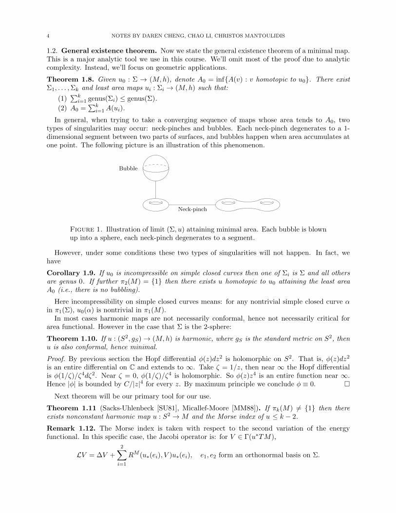
Theorem 1.8. Given u0 : Σ → (M,h), denote A0 = infA(v) : v homotopic to u0. There existΣ1, . . . ,Σk and least area maps ui : Σi → (M,h) such that:
(1)∑k
i=1 genus(Σi) ≤ genus(Σ).
(2) A0 =∑k
i=1A(ui).
In general, when trying to take a converging sequence of maps whose area tends to A0, twotypes of singularities may occur: neck-pinches and bubbles. Each neck-pinch degenerates to a 1-dimensional segment between two parts of surfaces, and bubbles happen when area accumulates atone point. The following picture is an illustration of this phenomenon.
Bubble
Neck-pinch
Figure 1. Illustration of limit (Σ, u) attaining minimal area. Each bubble is blownup into a sphere, each neck-pinch degenerates to a segment.
However, under some conditions these two types of singularities will not happen. In fact, wehave
Corollary 1.9. If u0 is incompressible on simple closed curves then one of Σi is Σ and all othersare genus 0. If further π2(M) = 1 then there exists u homotopic to u0 attaining the least areaA0 (i.e., there is no bubbling).
Here incompressibility on simple closed curves means: for any nontrivial simple closed curve αin π1(Σ), u0(α) is nontrivial in π1(M).
In most cases harmonic maps are not necessarily conformal, hence not necessarily critical forarea functional. However in the case that Σ is the 2-sphere:
Theorem 1.10. If u : (S2, gS)→ (M,h) is harmonic, where gS is the standard metric on S2, thenu is also conformal, hence minimal.
Proof. By previous section the Hopf differential φ(z)dz2 is holomorphic on S2. That is, φ(z)dz2
is an entire differential on C and extends to ∞. Take ζ = 1/z, then near ∞ the Hopf differentialis φ(1/ζ)/ζ4dζ2. Near ζ = 0, φ(1/ζ)/ζ4 is holomorphic. So φ(z)z4 is an entire function near ∞.Hence |φ| is bounded by C/|z|4 for every z. By maximum principle we conclude φ ≡ 0.
Next theorem will be our primary tool for our use.
Theorem 1.11 (Sacks-Uhlenbeck [SU81], Micallef-Moore [MM88]). If πk(M) 6= 1 then thereexists nonconstant harmonic map u : S2 →M and the Morse index of u ≤ k − 2.
Remark 1.12. The Morse index is taken with respect to the second variation of the energyfunctional. In this specific case, the Jacobi operator is: for V ∈ Γ(u∗TM),
LV = ∆V +
2∑i=1
RM (u∗(ei), V )u∗(ei), e1, e2 form an orthonormal basis on Σ.
286 - TOPICS IN DIFFERENTIAL GEOMETRY - LECTURE NOTES 5
Remark 1.13. Sacks-Uhlenbeck’s approach can be (very briefly) sketched as following. For α ≥ 1,define
Eα(u) =
ˆS2
(1 + ‖du‖2
)αda.
For α > 1, this is a ”good” variational problem and they are able to extract converging subsequencesof critical points of Eα.
Micallef-Moore further modify Eα to make its critical points non-degenerate, and they provedthe modified critical points also converge after passing to a subsequence.
Remark 1.14. We here point out that Colding and Minicozzi have a different approach for mini-mizers on S2, and X. Zhou generalized the result to higher genus surfaces.
2. Minimal submanifolds and Bernstein theorem
2.1. First variation of area functional. Let Σk ⊂ Mn be a submanifold. Denote by D theLevi-Civita connection on M and by h the vector valued second fundamental form
h(X,Y ) = (DXY )⊥, X, Y ∈ Γ(TM).
The vector
~H =k∑i=1
h(ei, ei)
is the mean curvature, where e1, . . . , ek is an orthonormal basis of tangent vector fields.Now if X is a vector field on M compactly supported on Σ and Ft is a flow with initial velocity
X, consider Σt = Ft(Σ). The variation of area functional can be calculated as following
δΣ(X) =d
dt
∣∣∣∣t=0
|Σt| =ˆ
ΣdivΣXdµ.
where divΣ(X) =∑k
i=1〈DeiX, ei〉 and dµ is the volume measure on Σ.
Decompose X into its tangent and normal components X = XT +X⊥, we may write 〈DeiX, ei〉 =〈DeiX
T , ei〉 + 〈DeiX⊥, ei〉. And the normal component can be further calculated as 〈DeiX, ei〉 =
−〈X⊥, (Dei , ei)⊥〉. Therefore
divΣ(X) = divΣ(XT )− 〈X, ~H〉.
And the first variation of area functional is δΣ(X) = −´
Σ〈X, ~H〉dµ.
Definition 2.1. Call Σk ⊂Mn minimal if ~H ≡ 0.
2.2. Second variation of area functional, Bernstein theorem. In many cases it’s necessaryto consider the second variation of area functional. We have
Proposition 2.2. Assume ~H ≡ 0 and Xp ⊥ TpΣ for every p on Σ, and X is compactly supportedon Σ. Then the second variation of area functional is given by
δ2Σ(X,X) =
ˆΣ‖D⊥X‖2 − ‖〈h,X〉‖2 −
k∑i=1
RM (ei, X, ei, X),
with e1, . . . , ek being an orthonormal basis on Σ.
Remark 2.3. We split TM = TΣ⊕NΣ. Then the ambient connection D gives rise to connectionson TΣ and NΣ. If Y ∈ Γ(TM) and X ∈ Γ(NM) then we have D⊥YX = (DYX)⊥. Then we
6 NOTES BY DAREN CHENG, CHAO LI, CHRISTOS MANTOULIDIS
may rewrite ‖D⊥X‖2 =∑k
i=1 ‖D⊥eiX‖2 and ‖〈h,X〉‖2 =
∑i,j〈hi,j , X〉2 = ‖DTX‖2, and the second
variation is given as
δ2Σ(X,X) =
ˆΣ‖D⊥X‖2 −
k∑i=1
RM (ei, X, ei, X)− ‖DTX‖2.
Definition 2.4. Define the Jacobi operator L on Γ(NΣ) by
LX = ∆⊥X +∑
RM (ei, X)ei +∑i,j
〈hij , X〉hij .
Then L is a second order self-adjoint operator on Γ(NΣ), and δ2Σ(X,X) = −´
Σ〈X,LX〉dµ.We call the number of negative eigenvalues of L the Morse index of Σ. Σ is called stable if the
Morse index is 0, strictly stable if there are also no Jacobi fields.
A famous and important question is to understand the structure of stable minimal surfaces. Thefirst important theorem is given by S. Berstein.
Theorem 2.5 (S. Berstein [Ber27]). Let Σ2 ⊂ R3 be a minimal surface and given by a graphx3 = u(x1, x2) defined for all (x1, x2). Then Σ is a plane; i.e., u must be a linear function.
Before proving Bernstein’s theorem, we first state some important properties of minimal graphsΣ = graph(u) in Rn+1, where u : Ω→ R is a C2 function.
Fact 2.6. Σ is 2-sided. That is, Σ has a unit normal vector field ν.
Fact 2.7. Σ is area minimizing in Ω× R.
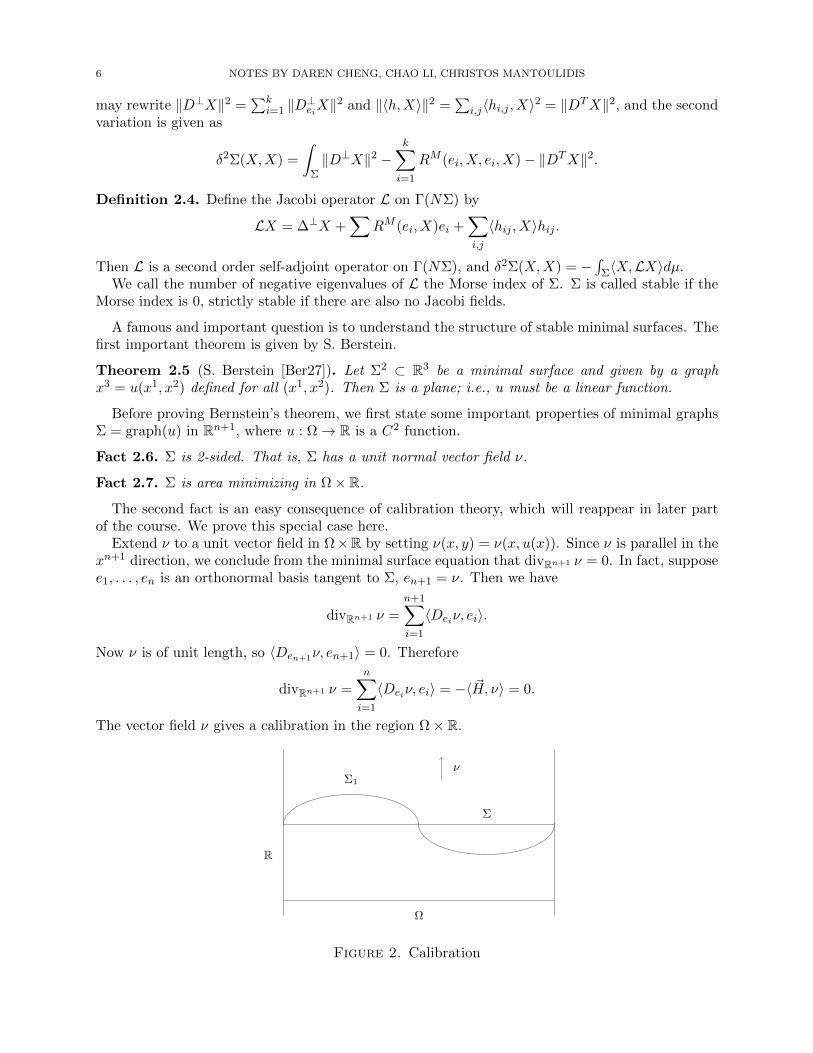
The second fact is an easy consequence of calibration theory, which will reappear in later partof the course. We prove this special case here.
Extend ν to a unit vector field in Ω×R by setting ν(x, y) = ν(x, u(x)). Since ν is parallel in thexn+1 direction, we conclude from the minimal surface equation that divRn+1 ν = 0. In fact, supposee1, . . . , en is an orthonormal basis tangent to Σ, en+1 = ν. Then we have
divRn+1 ν =
n+1∑i=1
〈Deiν, ei〉.
Now ν is of unit length, so 〈Den+1ν, en+1〉 = 0. Therefore
divRn+1 ν =n∑i=1
〈Deiν, ei〉 = −〈 ~H, ν〉 = 0.
The vector field ν gives a calibration in the region Ω× R.
Σ1
Σ
ν
Ω
R
Figure 2. Calibration
286 - TOPICS IN DIFFERENTIAL GEOMETRY - LECTURE NOTES 7
Suppose Σ1 ⊂ Ω×R and ∂Ω1 = ∂Ω. Denote ν1 the outer unit normal vector field on Ω1. Let Ω′
be the signed region in Rn+1 with Σ− Σ1 = ∂Ω′. Then by the divergence theorem,
0 =
ˆΩ′
divRn+1 ν =
ˆΣν · ν −
ˆΣ1
ν · ν1.
So we conclude
|Σ| =ˆ
Σν · ν =
ˆΣ1
ν · ν1 ≤ |Σ1|, by Cauchy-Schwarz.
Fact 2.8. If Σ is an entire minimal graph, then
|Σ ∩BR(0)| ≤ CRn, ∀R ≥ 1
This is an easy consequence of the fact that minimal graphs are area minimizing. Take anyR > 0. Then Σ divides ∂BR(0) = SR(0) into two parts Σ1,Σ2. Since Σ is a minimal graph overthe domain SnR(0) ⊂ Rn, we have
|Σ ∩BR(0)| ≤ min|Σ1|, |Σ2| ≤ CRn.
Now we prove Bernstein’s theorem through the following
Theorem 2.9. Assume Σ ⊂ R3 is stable, proper, orientable minimal surface with Euclidean areagrowth. That is, |Σ ∩BR(0)| ≤ CR2 for all R ≥ 1. Then Σ is a plane.
Proof. Take a normal vector field ν and let X = ϕν, ϕ ∈ C∞c (Σ). The stability condition gives
0 ≤ δ2Σ(X,X) =
ˆ‖∇ϕ‖2 − ‖h‖2ϕ2, where h is the scalar second fundamental form.
So we know ˆΣ‖h‖2ϕ2dµ ≤
ˆΣ‖∇ϕ‖2dµ, ∀ϕLipc(Σ).
We use the logarithmic cut-off trick. Denote ρ(x) = |x|, then ρ is a proper function on Σ and‖∇ρ‖2 ≤ ‖Dρ‖2 = 1. Define
ϕR(ρ) =
1 for ρ ≤ RlogR2/ρ
logR for R ≤ ρ ≤ R2
0 for ρ ≥ R2.
Claim:´
Σ ‖∇ϕR‖2 ≤ C(logR)−1.
In fact, we haveˆ
Σ∩(BR2−BR)‖∇ϕR‖2 ≤
ˆρ−2
(logR)2= (logR)−2
ˆ R2
Rr−2
(ˆρ=r
dσ
‖∇ρ‖
)dr.
The last equality is got by coarea formula. Here again we use coarea formula just for the constantfunction 1 on Σ ∩BR(0) to get ˆ
ρ=r
dσ
‖∇ρ‖=
d
dr|Σ ∩Br(0)|.
So ˆΣ∩(BR2−BR)
‖∇ϕR‖2 ≤ (logR)−2
(r−2|Σ ∩Br|
∣∣∣∣r=R2
r=R
+ 2
ˆ R3
Rr−3|Σ ∩Br(0)|dr
)≤ C1(logR)−2 + C2(logR)−1.
Here we used the area growth of Σ.
8 NOTES BY DAREN CHENG, CHAO LI, CHRISTOS MANTOULIDIS
Now take R to ∞ we getˆΣ∩BR(0)
‖h‖2dµ ≤ˆ
Σ∩BR2
‖h‖2ϕ2Rdµ ≤
ˆΣ∩(BR2−BR)
‖∇ϕR‖2dµ→ 0.
So h ≡ 0 and Σ is a plane.
Question 2.10. We are curious about possible generalization of Berstein’s theorem. The followingcases have been of great interest for researchers.
(1) For higher dimensional Σn ⊂ Rn+1 entire minimal graphs, can we conclude that Σ is affinespace? This question has been answered by many authors over many years. The conclusionis true for n ≤ 7 and false for n ≥ 8.
(2) Can we get a Berstein type theorem when Σn ⊂ Mn+1 where M is a curved manifold? Insome special cases this question can be answered. We’ll get back to this question later.
(3) For Σ2 ⊂ Rn where n ≥ 4, can we get a Bernstein type theorem? We’ll focus on thisdirection.
The third question is more complicated than it first appears. The fact is, we can constructa family of area minimizing surfaces in higher dimensional Euclidean spaces. Let n = 2m andJ : Rn → Rn being a complex structure, meaning J is orthogonal and J2 = −I. For each fixed Jtake Σ2 to be a J-holomorphic curve. Then Σ is area minimizing by a similar calibration argument.In particular, consider
Σ = (z, w) : w = f(z),Here f is a J-holomorphic function. Then Σ is an area-minimizing surface in R4.
3. Bernstein’s theorem in higher codimensions
As mentioned in the previous section, Bernstein’s theorem in its full generality fails in highercodimensions due to the presence of J-holomorphic curves, defined as follows.
Definition 3.1. Let n = 2m and let J be an orthogonal complex structure on Rn, i.e. an orthogonalmatrix J with J2 = −I. A J-holomorphic curve is a 2-dimensional surface Σ2 ⊆ Rn such that
J(TxΣ) = TxΣ, for all x ∈ Σ.
Proposition 3.2. J-holomorphic curves are area-minimizing among orientable competitors.
Proof. Consider the Kahler form ω, defined by ω(X,Y ) = JX ·Y . Since J is a constant matrix, weobserve that ω is closed. Next we show that ω is a calibrating form that restricts to the area formprecisely on J-invariant 2-planes. To see this, take any oriented 2-plane Π in Rn and let e1, e2be a positive orthonormal basis. By the Schwartz inequality,
|ω(e1, e2)| = |Je1 · e2| ≤ 1.
Moreover, ω(e1, e2) = 1 if and only if Je1 = e2, which is equivalent to the J-invariance of Π.To conclude the proof, let Σ0 be an oriented surface with ∂Σ0 = ∂Σ, then we can find a region
R with Σ− Σ0 = ∂R. Then we have
0 =
ˆRdω =
ˆ∂Rω =
ˆΣω −ˆ
Σ0
ω
= |Σ| −ˆ
Σ0
ω ≥ |Σ| − |Σ0|
and the proof is complete.
Since the hypotheses of Bernstein’s theorem certainly doesn’t rule out J-holomorphic curves,Proposition 3.2 shows that Bernstein’s theorem is generally false in higher codimensions. The bestone could hope for is perhaps the following statement.
286 - TOPICS IN DIFFERENTIAL GEOMETRY - LECTURE NOTES 9
Conjecture 3.3. Let Σ2 ⊆ Rn be a complete stable minimal surface, possibly with some controlledarea growth, then there exists 2k ≤ n and a 2k-plane P ⊆ Rn such that Σ is J-holomorphic in Pfor some complex structure J .
It turns out that even this is false in general. Nonetheless, all hope is not lost as there are someinteresting special cases in which Conjecture 3.3 is true. Below we list a few positive results.
(1) When n = 4 and Σ is oriented with area growth suitably bounded, the conjecture is true.(2) If genus(Σ) = 0 and ˆ
Σ(−K)da <∞,
then the conjecture is true for all n.(3) If the ambient space is replaced by Tn, then the conjecture is true for n = 4.
3.1. Complexifying the stability operator. We’ll treat the case (1). A key ingredient in theproof is a complexified version of the second variation formula. We first set up some notationsbefore writing down the formula. As before, let (Σ2, g) be an oriented surface in Mn. Around eachpoint of Σ we can find local isothermal coordinates (x1, x2), i.e.
g = λ2((dx1)2 + (dx2)2
), where λ2 =
∣∣∣∣ ∂∂x1
∣∣∣∣2 =
∣∣∣∣ ∂∂x2
∣∣∣∣2Next we write
(3.1)∂
∂z=
1
2
(∂
∂x1− i ∂
∂x2
);∂
∂z=
1
2
(∂
∂x1+ i
∂
∂x2
)Now recall that if Σ is minimal and X ∈ Γ(NΣ), then the second variation is given by
(3.2) δ2Σ(X,X) =
ˆΣ‖D⊥X‖2 −
2∑j=1
RM (ej , X, ej , X)− ‖DTX‖2da,
where ej is any orthonormal frame for TΣ. Now we complexify TΣ and NΣ and extend thesecond variation formula to complex vector fields. For X ∈ Γ(NCΣ), we simply write
(3.3) δ2Σ(X,X) =
ˆΣ‖D⊥X‖2 −
2∑j=1
RM (ej , X, ej , X)− ‖DTX‖2da
Of course now ‖D⊥X‖2 = 〈D⊥X,D⊥X〉 and likewise for ‖DTX‖2. Below we’ll use the operators(3.1) to rewrite (3.3). More precisely, we have the following formula.
Proposition 3.4. Let Σ2 and Mn be as above and let X ∈ Γ(NCΣ), then
(3.4) δ2Σ(X,X) = 4
ˆΣ‖D⊥∂
∂z
X‖2 −RM (∂
∂z,X,
∂
∂z,X)− ‖DT
∂∂z
X‖2dx1 ∧ dx2,
Remark 3.5. Notice that the integrand[‖D⊥∂
∂z
X‖2 −RM (∂
∂z,X,
∂
∂z,X)− ‖DT
∂∂z
X‖2]dx1 ∧ dx2
is conformally invariant. Thus, even though it’s written in terms of coordinates, it makes senseglobally on Σ.
Proof.
10 NOTES BY DAREN CHENG, CHAO LI, CHRISTOS MANTOULIDIS
1. We start from (3.3). Introducing isothermal coordinates as above, the area element dabecomes λ2dx1 ∧ dx2. Plugging this into (3.2) and using the orthonormal frame ej =
λ−1 ∂∂xj
, j = 1, 2, we find that
(3.5) δ2Σ(X,X) =
ˆΣ
2∑j=1
‖D⊥∂∂xjX‖2 −
2∑j=1
RM (∂
∂xj, X,
∂
∂xj, X)−
2∑j=1
‖DT∂
∂xjX‖2dx1 ∧ dx2
2. Next we notice that
‖D⊥∂∂z
X‖2 + ‖D⊥∂∂z
X‖2 =1
4〈D⊥∂
∂x1X − iD⊥∂
∂x2X, D⊥∂
∂x1X + iD⊥∂
∂x2X〉
+1
4〈D⊥∂
∂x1X + iD⊥∂
∂x2X, D⊥∂
∂x1X − iD⊥∂
∂x2X〉
=1
2
(‖D⊥∂
∂x1X‖2 + ‖D⊥∂
∂x2X‖2
)Likewise, we also have
‖DT∂∂z
X‖2 + ‖DT∂∂z
X‖2 =1
2
(‖DT
∂∂x1
X‖2 + ‖DT∂
∂x2X‖2
)and
RM (∂
∂z,X,
∂
∂z,X) +RM (
∂
∂z,X,
∂
∂z,X)
=1
2
(RM (
∂
∂x1, X,
∂
∂x1, X) +RM (
∂
∂x2, X,
∂
∂x2, X)
)Plugging these into (3.5), we obtain
δ2Σ(X,X) = 2
ˆΣ‖D⊥∂
∂z
X‖2 + ‖D⊥∂∂z
X‖2 −RM (∂
∂z,X,
∂
∂z,X)
+RM (∂
∂z,X,
∂
∂z,X)− ‖DT
∂∂z
X‖2 − ‖DT∂∂z
X‖2dx1 ∧ dx2(3.6)
3. Take the term´
Σ ‖D⊥∂∂z
X‖2dx1 ∧ dx2. We want to integrate by parts to write it in terms of´Σ ‖D
⊥∂∂z
X‖2dx1 ∧ dx2, a curvature term and some other stuff. To do so, we observe
‖D⊥∂∂z
X‖2 = ‖D ∂∂zX‖2 − ‖DT
∂∂z
X‖2
= 〈D ∂∂zX, D ∂
∂zX〉 − ‖DT
∂∂z
X‖2
=∂
∂z〈D ∂
∂zX, X〉 − 〈D ∂
∂zD ∂
∂zX, X〉 − ‖DT
∂∂z
X‖2
=∂
∂z〈D ∂
∂zX, X〉 − 〈D ∂
∂zD ∂
∂zX, X〉 −RM (
∂
∂z,∂
∂z,X,X)− ‖DT
∂∂z
X‖2
=∂
∂z〈D ∂
∂zX, X〉 − ∂
∂z〈D ∂
∂zX, X〉+ 〈D ∂
∂zX, D ∂
∂zX〉 −RM (
∂
∂z,∂
∂z,X,X)− ‖DT
∂∂z
X‖2
=∂
∂z〈D ∂
∂zX, X〉 − ∂
∂z〈D ∂
∂zX, X〉+ ‖D⊥∂
∂z
X‖+ ‖DT∂∂z
X‖2 −RM (∂
∂z,∂
∂z,X,X)− ‖DT
∂∂z
X‖2(3.7)
Integrating over Σ, using the fact that X has compact support and plugging into (3.6), weget
δ2Σ(X,X) = 2
ˆΣ
2‖D⊥∂∂z
X‖2 −RM (∂
∂z,∂
∂z,X,X)−RM (
∂
∂z,X,
∂
∂z,X)
286 - TOPICS IN DIFFERENTIAL GEOMETRY - LECTURE NOTES 11
−RM (∂
∂z,X,
∂
∂z,X)− 2‖DT
∂∂z
X‖2dx1 ∧ dx2(3.8)
By the first Bianchi identity,
RM (∂
∂z,∂
∂z,X,X) +RM (
∂
∂z,X,
∂
∂z,X) = −RM (X,
∂
∂z,∂
∂z,X) = RM (
∂
∂z,X,
∂
∂z,X).
Therefore from (3.8) we get
δ2Σ(X,X) = 2
ˆΣ
2‖D⊥∂∂z
X‖2 − 2RM (∂
∂z,X,
∂
∂z,X)− 2‖DT
∂∂z
X‖2dx1 ∧ dx2
= 4
ˆΣ‖D⊥∂
∂z
X‖2 −RM (∂
∂z,X,
∂
∂z,X)− ‖DT
∂∂z
X‖2dx1 ∧ dx2
as stated. The proof is now complete.
In the case where the ambient manifold is Rn, (3.4) simplifies and we have the following beautifulstability criterion.
Corollary 3.6. Suppose Σ2 ⊆ Rn is a stable oriented minimal surface, then
(3.9)
ˆΣ‖DT
∂∂z
X‖2dx1 ∧ dx2 ≤ˆ
Σ‖D⊥∂
∂z
X‖2dx1 ∧ dx2, for all X ∈ Γ(NCΣ)
Proof. Each section X ∈ Γ(NCΣ) can be written as X = X1 + iX2, where X1, X2 are sections ofthe real normal bundle NΣ. Then we have
δ2Σ(X,X) = δ2Σ(X1, X1) + δ2(X2, X2) ≥ 0,
where the last inequality is true by stability. The corollary now follows from Proposition 3.4.
3.2. Stable minimal surfaces in R4 and T 4. Let’s come back to complete oriented stable min-imal surfaces in R4. Recall that our goal is to construct an orthogonal complex structure J onR4 with respect to which Σ is holomorphic. We introduce some notations before describing theconstruction. We will roughly be following [Mic84].
For clarity, below we suppose Σ is the image of an isometric stable minimal immersion F : M2 →R4, where M2 is a complete oriented surface. Let E 'M ×R4 denote the pullback of TR4 and itsmetric structure via F . Then we can view TM as a sub-bundle of E and use the metric to definethe orthogonal complement bundle, which we denote by NM . Since M is oriented, the pullbackmetric induces a complex structure JT on M . Also, still by orientability, we can define a complexstructure J⊥ on NM by rotation by 90 in the clockwise or counterclockwise direction (notice thatwe have a choice here). We then define J : M → Hom(E) as follows: for each p ∈ M , given avector v ∈ Ep, we define,
Jp(v) = JTp (vT ) + J⊥p (v⊥),
where vT and v⊥ denote the orthogonal projections of v onto TpM and NpM , respectively.The triviality of E allows us to view J as a map from M to Hom(R4). What we want to
demonstrate now is that J is constant, so that J : M → Hom(R4) extends as a complex structureon all of R4. To see this, we first complexify E, TM and NM and extend JT and J⊥ to be complexlinear maps. Then JT gives rise to a splitting
TCM = T 1,0M ⊕ T 0,1M.
Likewise, NCM splits as N1,0M ⊕N0,1M . We denote N1,0M by V ; then N0,1M = V . With thesenotations, we form the following sub-bundle of EC 'M × C4:
W = T 1,0M ⊕ V.
12 NOTES BY DAREN CHENG, CHAO LI, CHRISTOS MANTOULIDIS
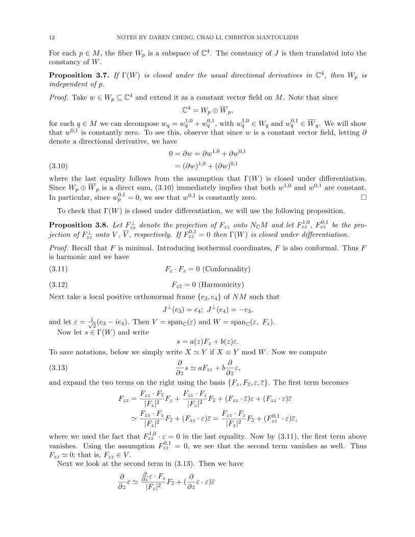
For each p ∈ M , the fiber Wp is a subspace of C4. The constancy of J is then translated into theconstancy of W .
Proposition 3.7. If Γ(W ) is closed under the usual directional derivatives in C4, then Wp isindependent of p.
Proof. Take w ∈Wp ⊆ C4 and extend it as a constant vector field on M . Note that since
C4 = Wp ⊕W p,
for each q ∈M we can decompose wq = w1,0q +w0,1
q , with w1,0q ∈Wq and w0,1
q ∈W q. We will showthat w0,1 is constantly zero. To see this, observe that since w is a constant vector field, letting ∂denote a directional derivative, we have
0 = ∂w = ∂w1,0 + ∂w0,1
= (∂w)1,0 + (∂w)0,1(3.10)
where the last equality follows from the assumption that Γ(W ) is closed under differentiation.Since Wp ⊕W p is a direct sum, (3.10) immediately implies that both w1,0 and w0,1 are constant.
In particular, since w0,1p = 0, we see that w0,1 is constantly zero.
To check that Γ(W ) is closed under differentiation, we will use the following proposition.
Proposition 3.8. Let F⊥zz denote the projection of Fzz onto NCM and let F 1,0zz , F 0,1
zz be the pro-
jection of F⊥zz onto V , V , respectively. If F 0,1zz = 0 then Γ(W ) is closed under differentiation.
Proof. Recall that F is minimal. Introducing isothermal coordinates, F is also conformal. Thus Fis harmonic and we have
(3.11) Fz · Fz = 0 (Conformality)
(3.12) Fzz = 0 (Harmonicity)
Next take a local positive orthonormal frame e3, e4 of NM such that
J⊥(e3) = e4; J⊥(e4) = −e3,
and let ε = 1√2(e3 − ie4). Then V = spanC(ε) and W = spanC(ε, Fz).
Now let s ∈ Γ(W ) and writes = a(z)Fz + b(z)ε.
To save notations, below we simply write X ' Y if X ≡ Y mod W . Now we compute
(3.13)∂
∂zs ' aFzz + b
∂
∂zε,
and expand the two terms on the right using the basis Fz, Fz, ε, ε. The first term becomes
Fzz =Fzz · Fz|Fz|2
Fz +Fzz · Fz|Fz|2
Fz + (Fzz · ε)ε+ (Fzz · ε)ε
' Fzz · Fz|Fz|2
Fz + (Fzz · ε)ε =Fzz · Fz|Fz|2
Fz + (F 0,1zz · ε)ε,
where we used the fact that F 1,0zz · ε = 0 in the last equality. Now by (3.11), the first term above
vanishes. Using the assumption F 0,1zz = 0, we see that the second term vanishes as well. Thus
Fzz ' 0; that is, Fzz ∈ V .Next we look at the second term in (3.13). Then we have
∂
∂zε '
∂∂z ε · Fz|Fz|2
Fz + (∂
∂zε · ε)ε
286 - TOPICS IN DIFFERENTIAL GEOMETRY - LECTURE NOTES 13
=∂∂z ε · Fz|Fz|2
Fz (ε had unit length)
= −ε · Fzz|Fz|2
Fz (integrate by parts in the first term)
= −ε · F0,1zz
|Fz|2Fz (F 1,0
zz · ε = 0)
= 0 (by assumption) .
Thus for each section s of W , we’ve shown that ∂∂zs ' 0. Similarly we can show that ∂
∂zs ' 0.Thus Γ(W ) is preserved by differentiation.
To verify the assumption of Proposition 3.8, we suppose in addition that M is parabolic.
Definition 3.9. Given a Riemannnian surface M , we say that M is parabolic if every positivesuperharmonic function on M is constant.
Below we give some examples of parabolic manifolds.
Example 3.10.
(1) The complex plane C is parabolic. On the other hand, the unit disk D ⊂ C is not parabolic.(2) Any compact Riemann surface with finitely many punctures is parabolic.(3) If M is a complete surface with |M ∩BR| ≤ CR2 for R large, then M is parabolic.
Proof. Suppose u > 0 is a positive superharmonic function on M . Letting w = log u, wehave
∆w =∆u
u− |∇u|
2
u2≤ ∆u
u− |∇w|2
≤ −|∇w|2 (since ∆u ≤ 0) .(3.14)
Next we test the inequality (3.14) against ϕ2, where ϕ is any test function ϕ ∈ C1C(M),
getting ˆMϕ2|∇w|2d vol ≤ −
ˆMϕ2∇wd vol = 2
ˆMφ〈∇ϕ,∇w〉d vol
≤ 1
2
ˆMϕ2|∇w|2d vol +2
ˆM|∇ϕ|2d vol
Hence we get ˆMϕ2|∇w|2d vol ≤ 4
ˆM|∇ϕ|2d vol .
Applying the logarithmic cut-off trick as in the proof of the Bernstein theorem in the lastsection, we conclude that w, and thus u, is constant.
(4) If Σ2 ⊆ Rn is an entire minimal graph, then Σ with the induced metric is parabolic.
Proof. We will prove that Σ is conformally equivalent to C. By the uniformization theorem,we know that Σ is conformally equivalent either to C or to D. Assume by contradictionthat the latter holds and let F : D → Σ be a biholomorphic map. Since Σ is isometricallyand minimally embedded, F is harmonic as a map of D into Rn. Modifying F by anautomorphism of D is necessary, we may assume that F (0) = (0, 0, u(0, 0)).
Next denote F (x1, x2) = (F1(x1, x2), F2(x1, x2)). By the previous paragraph, F is aharmonic diffeomorphism from D to (R2, h), where h is obtained by pulling back the inducedmetric on Σ via (x1, x2) 7→ (x1, x2, u(x1, x2)).
14 NOTES BY DAREN CHENG, CHAO LI, CHRISTOS MANTOULIDIS
Recall that in complex coordinates, the Jacobian of F can be written as
(3.15) J(F ) = |Fz|2 − |Fz|2,
which is everywhere strictly positive since F is a diffeomorphism. This implies that |Fz| iseverywhere non-zero, so we can define a metric g on D by
g = |Fz|2|dz|2.
Now since F is harmonic, we have Fzz = 0 and hence ∆|Fz|2 = 0, which means that (D, g)is flat (Gauss curvature zero).
Using (3.15) again, we see that |dF | is dominated by |Fz| and hence
F ∗(h) ≤ cg,where c is a dimensional constant. Now for an arbitrary R > 0, we can choose r such that
distF ∗(h)(0, ∂Dr) = disth(0, ∂(F (Dr))) ≥ R.
Combining this with the previous inequality, we get
(3.16) cdistg(0, ∂Dr) ≥ RNext we take the coordinate function x on D. Then
∆gx = 0|x| ≤ 1
so by the harmonic function estimates in [CY75] and the definition of g, we have
1
|Fz|2= |∇gx|2(0) ≤ c
distg(0, ∂Dr)2≤ c
R2.
This in turn gives us
|dF |2(0) ≥ |Fz|2(0) ≥ cR2.
Since R is arbitrary, we obtain a contradiction, so Σ is conformally equivalent to C andhence parabolic.
After this little digression into parabolic manifolds we return to our problem and give the precisestatement of the main result of this section.
Theorem 3.11. Assume F : M2 → R4 is an oriented, stable, parabolic, complete minimal surface.Then F is J-holomorphic for some orthogonal complex structure J on R4.
Proof. By Proposition 3.8, the proof reduces to showing that F 0,1zz vanishes. We will demonstrate
this by plugging special test functions into the stability inequality (3.4) and using parabolicity. Tothat end we consider a test function of the form fs, where f is a real-valued smooth function withcompact support on M , and s ∈ Γ(NCM). Then we have
(3.17) δ2Σ(fs, fs) =
ˆM|fz|2|s|2 − f2(Re〈s,Dzzs〉)− f2|(∂Tz s)|2dx1 ∧ dx2,
where we’re using D to denote D⊥. To derive this formula, we recall that by (3.4) we have
(3.18) δ2Σ(fs, fs) =
ˆM|Dz(fs)|2 − |∂Tz (fs)|2dx1 ∧ dx2
To handle the first term we computeˆ|Dz(fs)|2 =
ˆDz(fs) ·Dz(fs) =
ˆ(fzs+ fDzs) · (fzs+ fDzs)
=
ˆ|fz|2|s|2 + f2|Dzs|2 + ffzDzs · s+ (complex conjugate of the previous term)
286 - TOPICS IN DIFFERENTIAL GEOMETRY - LECTURE NOTES 15
=
ˆ|fz|2|s|2 + f2|Dzs|2 + 2Re(ffzDzs · s)(3.19)
Now notice that ˆffzDzs · s =
1
2
ˆ(f2)zDzs · s
= −1
2
ˆf2DzDzs · s−
1
2
ˆf2|Dzs|2
Plugging this back into (3.19), we get
(3.20)
ˆ|Dz(fs)|2 =
ˆ|fz|2|s|2 − f2Re(Dzzs · s)
For the second term in (3.18), we notice that
∂z(fs) = fzs+ f∂zs.
Since s is a normal section, projection onto TM kills the first term and we’re left with
(3.21) ∂Tz (fs) = f(∂Tz s)
(3.17) now follows by plugging (3.20) and (3.21) back into (3.18). To proceed, we take a vectora ∈ C4 and denote by a1,0(p) its projection onto Vp. Applying (3.17) with a1,0 in place of s andusing the stability of M in R4, the result we get is the following
(3.22)
ˆMf2q(a)dA ≤
ˆM|∇f |2|a1,0|2dA ≤ |a|
ˆM|∇f |2dA,
where q is the following expression:
(3.23) q(a) =−2
|Fz|4Re
(F 1,0zz · a)(F 1,0
zz · a).
Take an orthonormal basks a1, . . . , a4 of C4, denote q(aj) by qj and sum over j, we obtain
(3.24)4∑j=1
qj =−2
|Fz|4ReF 1,0zz · F
1,0zz
= 0
Now by [FCS80], the inequality (3.22) with qj in place of q(a) implies the existence of a positivefunction uj on M solving
(3.25) ∆uj + qjuj = 0
Letting wj = log uj , an easy calculation shows that
∆wj = −qj − |∇wj |2.Thus we get ˆ
M(qj + |∇wj |2)f2 =
ˆM
(−∆wj)f2 = 2
ˆMf∇f · ∇wj
≤ 1
2
ˆMf2|∇wj |2 + 2
ˆM|∇f |2,
and therefore ˆM
(qj +1
2|∇wj |2)f2 ≤ 2
ˆM|∇f |2
Summing over j and using (3.24), we deduce that
1
2
ˆM
4∑j=1
|∇wj |2f2 ≤ 8
ˆM|∇f |2.
16 NOTES BY DAREN CHENG, CHAO LI, CHRISTOS MANTOULIDIS
Again by [FCS80], we get a positive function v such that
8∆v +1
2(
4∑j=1
|∇wj |2)v = 0
⇒ ∆v ≤ 0;
that is v is a positive superharmonic function. By the parabolicity of M , v must be a (nonzero)
constant. Looking back at the PDE satisfied by v, we immediately deduce that4∑j=1|∇wj |2 = 0, so
each wj , and hence each uj , is constant. By (3.25), we see that each qj is zero. Since the aj ’s forma basis for C4, we conclude that
(3.26) q(a) =−2
|Fz|4Re
(F 1,0zz · a)(F 1,0
zz · a)
= 0, for all a ∈ C4.
Now at a point p where F⊥zz(p) 6= 0, we can let a =F⊥zz|F⊥zz |
and plug it into (3.26). Then we get
(3.27) |F 1,0zz (p)||F 0,1
zz (p)| = 0.
Thus at each p ∈ M , one of F 1,0zz (p) and F 0,1
zz (p) must vanish. The fact that F is conformal and
harmonic implies that F 1,0zz dz2 and F 0,1
zz dz2 are holomorphic quadratic differentials with values in Vand V , respectively. Hence we conclude, by unique continuation, that either F 1,0
zz or F 0,1zz vanishes
identically. In the latter case, the proof is complete by invoking Proposition 3.8. In the formercase we simply change the complex structure J⊥ on NM . (Recall that we had a choice whenconstructing J⊥. See the remarks before Proposition 3.7.)
More or less the same argument establishes the same theorem in the compact setting of ambientflat 4-tori instead of R4.
Theorem 3.12. Assume F : M2 → T 4 is an oriented, stable, compact minimal surface and thatT 4 is a flat torus. Then F is J-holomorphic for some orthogonal complex structure J on T 4.
Proof sketch. By arguing as in 3.11 we get λ0(∆ + qj) ≥ 0 on M for all j ∈ 1, 2, 3, 4. Letuj = ewj > 0 be the lowest eigenfunction so that, as before,ˆ
M(qj +
1
2|∇wj |2)f2 ≤ 2
ˆM|∇f |2 for j ∈ 1, 2, 3, 4.
Summing over j and recalling the definition of the qj we conclude
1
2
ˆM
∑j
|∇wj |2f2 ≤ 8
ˆM|∇f |2.
Picking f = 1 (since M compact) we see that each wj is constant, so each uj is constant, soqj = λ0(∆ + qj) is constant. Since the qj sum to zero they must then all be zero and the resultfollows like before.
In the proof of Theorem 3.11 we made use of identity (3.23) in (3.22). Let’s justify that now:
Claim 3.13. We can rewrite
2
|Fz|2
[|a1,0 · Fzz|2
|Fz|2+ Re
(a1,0 ·DzDza
1,0)]
= − 2
|Fz|4Re(
(F 1,0zz · a)(F 1,0
zz · a))
where a ∈ C4, |a| = 1.
286 - TOPICS IN DIFFERENTIAL GEOMETRY - LECTURE NOTES 17
Proof of claim. Recall that ε = 1√2(e3 − ie4) is such that ε, ε forms an orthonormal frame for
NCM = V ⊕ V . Note that ε · ε = ε · ε = 0 and ε · ε = 1. By differentiating a1,0 = (a · ε)ε once andusing the product rule,
Dza1,0 = ∂z(a · ε)ε+ (a · ε)Dzε
= (a · (∂zε)T )ε+ (a ·Dzε)ε+ (a · ε)[(Dzε · ε)ε+ (Dzε · ε)ε
]= (a · (∂zε)T )ε+
[a ·((Dzε · ε)ε+ (Dzε · ε)ε
)]ε+ (a · ε)
[(Dzε · ε)ε+ (Dzε · ε)ε
]= (a · (∂zε)T )ε+ (a · ε)(Dzε · ε)ε+ (a · ε)(Dzε · ε)ε,
because Dzε · ε = Dzε · ε = 0, as ε · ε = ε · ε = 0
= (a · (∂zε)T )ε,
because ε · ε = 1
=[a ·((∂zε · (Fz/|Fz|2))Fz + (∂zε · (Fz/|Fz|2))Fz
)]ε
= −(a · Fz|Fz|2
)(ε · Fzz) ε.(3.28)
where the last equality follows from the product rule and minimality, Fzz = 0. We will differentiateagain in z, but before doing so, first we observe that
∂z
(Fz|Fz|2
)· Fz = 0 by conformality, Fz · Fz = 0, and
∂z
(Fz|Fz|2
)· Fz = 0 by minimality, Fzz = 0.
Consequently, ∂z(Fz/|Fz|2) is purely normal and thus
∂z
(Fz|Fz|2
)=
F⊥zz|Fz|2
.
Plugging this into (3.28) and exploiting similar cancelations among the derivatives of ε, ε, we get
DzDza1,0 = −
(a · F
⊥zz
|Fz|2
)(ε · Fzz) ε = −
(a · F
⊥zz
|Fz|2
)F 1,0zz
and
a1,0 ·DzDza1,0 = −
(a · F
⊥zz
|Fz|2
)(a1,0 · F 1,0
zz ) = −(a · F
⊥zz
|Fz|2
)(a · F 1,0
zz )
by replacing a1,0 with a in the dot product with F 1,0zz . By replacing F⊥zz = F 1,0
zz + F 0,1zz and then
using F 0,1zz = F 1,0
zz we get
a1,0 ·DzDza1,0 = −a · F
1,0zz
|Fz|2(a · F 1,0
zz )− a · F 0,1zz
|Fz|2(a · F 1,0
zz )
= −a · F1,0zz
|Fz|2(a · F 1,0
zz )− |a · F0,1zz |2
|Fz|2
= −a · F1,0zz
|Fz|2(a · F 1,0
zz )− |a1,0 · Fzz|2
|Fz|2.
18 NOTES BY DAREN CHENG, CHAO LI, CHRISTOS MANTOULIDIS
From this we conclude
Re
(a1,0 ·DzDza
1,0 +|a1,0 · Fzz|2
|Fz|2
)= − 1
|Fz|2Re(
(a · F 1,0zz )(a · F 1,0
zz ))
which gives the required result.
3.3. Stable minimal genus-0 surfaces in Rn, n ≥ 5. We now try to see what we can provewhen R4 (or T 4) is replaced by Rn, n ≥ 5. We will show that:
Theorem 3.14. Let F : M2 → Rn, n ≥ 5, with M complete, oriented, stable, genus 0, and finitetotal curvature. Then there exists an affine subspace A2k ⊂ Rn such that F is J-holomorphic forsome J .
Remark 3.15. The requirement of finite total curvature might appear to be too strong but in factit isn’t. One can check using Gauss-Bonnet that, provided F is proper,
quadratic area growth, |χ(M)| <∞⇔ finite total curvature.
We will appeal to a theorem by Chern and Osserman [CO67]:
Theorem 3.16 ([CO67]). Suppose M2 ⊂ Rn is a complete orientable minimal surface with finitetotal curvature, i.e., ˆ
M(−K) dA <∞.
Then M is conformally equivalent to a punctured compact surface M and the Gauss map extendsthrough the punctures, meaning p 7→ TpM , NpM extend smoothly to M .
We will also need the following consequence of the stability inequality
(3.29) 2
ˆM
[f2 |(∂zs)T |2
|Fz|2+
f2
|Fz|2Re (s ·DzDzs)
]dA ≤
ˆM
ˆ|∇f |2 |s|2 dA,
for all f ∈ C∞c (M).
Lemma 3.17. Suppose M is complete, oriented, stable, parabolic, and that s is a bounded sectionof NCM with Dzs = 0. Then (∂zs)
T = 0.
Proof. From (3.29) with Dzs = 0 and |s| bounded we conclude thatˆMf2 |(∂zs)T |2
|Fz|2dA ≤ c
ˆM|∇f |2 dA
for all f , so by elliptic theory there exists u > 0 with
∆u+|(∂zs)T |2
c|Fz|2u = 0.
By parabolicity u needs to be constant, and therefore (∂zs)T = 0.
Proof of Theorem 3.14. By invoking the Chern-Osserman theorem we can construct a complex(n− 2)-plane bundle E → M extending NCM , where M ≈ S2 in view of our genus 0 assumption,and we can also extend the connection D from before to a connection on E.
By [KM58] and the fact that dimM = 2 it follows that E is a holomorphic vector bundle; i.e.,for all p ∈ S2 there exists a local basis s1, . . . , sn−2 of E which is holomorphic (Dzsj = 0). By[Gro57], the holomorphic vector bundle E necessarily decomposes as a direct sum
E = (L1 ⊕ · · · ⊕ Lp)⊕ (Lp+1 ⊕ · · · ⊕ Lr)⊕ (Lr+1 ⊕ · · · ⊕ Ln−2)
of complex line bundles order so that:
(1) L1, . . . , Lp have c1(L) > 0,
286 - TOPICS IN DIFFERENTIAL GEOMETRY - LECTURE NOTES 19
(2) Lp+1, . . . , Lr have c1(L) = 0, and(3) Lr+1, . . . , Ln−2 have c1(L) < 0.
Roughly speaking, we will show that if there are no flat bundles then F is going to be J-holomorphic; conversely, flat bundles will correspond to direction of vanishing of the second funda-mental form and will help determine the affine space A2k from the statement of the theorem.
Seeing as to how E was initially constructed as a complexification of a real bundle, the real pairingEx × Ex → R, (s1, s2) 7→ s1 · s2, gives rise to a holomorphic isomorphism E ∼= E∗. According tothis isomorphism the signs of the first Chern classes flip and therefore our original decompositionhas to have as many positive line bundles as it does negative ones; namely, p = n− 2− r.
By definition of c1(·), the bundles L1, . . . Lr (whose first Chern class is non-negative) all ad-mit nontrivial global holomorphic sections s1, . . . , sn−2. Since S2 is compact, these sections areadditionally bounded. By Lemma 3.17 above, (∂zsj)
T = 0 for all j ∈ 1, . . . , r.There are two cases to consider. First, suppose that all Li have c1 = 0. Then s1, . . . , sn−2 is a
global basis of holomorphic sections which we have showed satisfy (∂zsj)T = 0 and therefore the
second fundamental form of M vanishes:
s =∑j
ajsj ⇒ −(s · F⊥zz)Fz|Fz|2
=∂zs · Fz|Fz|2
= (∂zs)T = 0.
Therefore M is totally geodesic and we’re done.Now suppose that p > 0, n − 2 − r = p > 0. For convenience we set up the following table of
index notation:
1 ≤ µ, ν ≤ p, r + 1 ≤ a, b ≤ n− 2,
1 ≤ i, j ≤ r, p+ 1 ≤ A,B ≤ n− 2.
In other words, indices µ, ν run over positive line bundles, i, j run over non-negative line bundles,and so on. We list some properties of s1, . . . , sn−2 that we will need.
(1) sµ · sj = 0, since∂z(sµ · sj) = Dzsµ · sj + sµ ·Dzsj = 0
because we know that our sections are holomorphic. Therefore sµ · sj is a holomorphicfunction on S2, thus constant. However, the section sµ belongs to a positive line bundleand necessarily vanishes somewhere. The claim follows. As a consequence, we get:
(3.30) spanL1, . . . , Lr⊥ = spanL1, . . . , Lp.(2) ∂zsj · sk = 0, since
∂z(∂zsj · sk) = ∂z∂zsj · sk + ∂zsj · ∂zsk= ∂z(∂zsj · sk)− ∂zsj · ∂zsk + ∂zsj · ∂zsk.
Since sj is holomorphic, ∂zsj is purely tangential so the first term drops out by orthogonality.Next, sk is a bounded holomorphic section so by Lemma 3.17 (which relies on stability),∂zsk is purely normal, the second term drops out by orthogonality. The same goes for thethird term. Therefore the expression above vanishes, so ∂zsj ·skdz is a holomorphic 1-form.The claim follows since Riemann-Roch forces such a differential to vanish identically. Fromthis it follows that ∂zsj ∈ spanL1, . . . , Lp, and since (∂zsj · sk)T = 0 by stability (Lemma3.17), we get
(3.31) ∂zsj , Dzsj ∈ spanL1, . . . , Lp.Now we check the following
Claim 3.18. The bundle ξ = L1 ⊕ · · · ⊕ Lr ⊕ (TCM)1,0 is parallel.
20 NOTES BY DAREN CHENG, CHAO LI, CHRISTOS MANTOULIDIS
Proof of claim. By Proposition 3.7 we need to check that ∂z, ∂z map Γ(ξ) into itself. By linearitythis amounts to showing
∂zsj , ∂zsj , ∂zFz, ∂zFz ∈ Γ(ξ).
By minimality ∂zFz ∈ Γ(ξ) is clear, while ∂zsj ∈ Γ(ξ) is just (3.31). For the other two cases wecompute
∂zsj = (∂zsj)T because Dzsj = 0 by holomorphicity
=
(∂zsj ·
Fz|Fz|2
)Fz +
(∂zsj ·
Fz|Fz|2
)Fz
=
(∂zsj ·
Fz|Fz|2
)Fz,
the last equality following from minimality, Fzz = 0, and therefore ∂zsj ∈ Γ(ξ). Likewise we find
∂zFz =
(∂zFz ·
Fz|Fz|2
)Fz +
(∂zFz ·
Fz|Fz|2
)Fz + (∂zFz)
⊥
=
(∂zFz ·
Fz|Fz|2
)Fz + (∂zFz)
⊥,
seeing as to how the first term drops out in view of conformality, Fz · Fz = 0. Now we observe∂zFz · sk = −Fz · ∂zsk = 0 by stability, and we conclude ∂zFz ∈ Γ(ξ). This completes the proof ofthe claim.
Next we check the following
Claim 3.19. We have dim(ξ ∩ ξ) = r − p.
Proof of claim. Recall that ξ = L1 ⊕ · · · ⊕ Lr ⊕ (TCM)1,0. For brevity write V = L1 ⊕ · · · ⊕ Lr, sothat ξ = V ⊕ (TCM)1,0. From (3.30) we see that V ⊥ ⊂ V , so spanξ, ξ = Cn. Observe that
n = dimCn = dim spanξ, ξ = 2r + 2− dim(ξ ∩ ξ)
which gives dim(ξ∩ξ) = 2r+2−n. From the decomposition of E into line bundles by Grothendieck’stheorem we further have p+ r = n−2⇔ r = n−2−p. Combining these two relations we conclude
dim(ξ ∩ ξ) = 2(n− 2− p) + 2− n = n− 2− 2p = r − p
which is the required result.
The proof of the theorem is now completed via the following sequence of steps:
(1) Since ξ is parallel, let’s write ξ = M × Λ for a complex (r + 1)-dimensional vector spaceΛ. Notice that the complex (r − p)-dimensional vector space T = Λ ∩ Λ is (by definition)preserved by complex conjugation and therefore the complexification W ⊗R C of a real(r − p)-dimensional vector space W .
(2) Seeing as to how (TCM)1,0 is manifestly not preserved by conjugation we get that M ×Wis a parallel subbundle of the real normal bundle NM , or in other words, that Σ = F (M)is a subset of an affine subspace P ⊂ Rn perpendicular to W , the dimension of which isevidently dimRn−dimW = n− (r− p) = n− r+ p = 2p+ 2. That is, we have constructedan affine subspace P 2p+2 ⊂ Rn that contains the surface Σ.
(3) From the decomposition NCM = (M × T ) ⊕ (M × T )⊥, the ⊥ being taken within NCMof course, we characterize (M × T )⊥ as the complexified normal bundle of Σ viewed as asurface within P 2p+2.
286 - TOPICS IN DIFFERENTIAL GEOMETRY - LECTURE NOTES 21
(4) From (3.30) we find that (M × T )⊥ ⊂ L1 ⊕ · · · ⊕ Lp ⊕ L1 ⊕ · · · ⊕ Lp and, by dimensioncounting, this inclusion is actually an exact equality. Namely,
(M × T )⊥ = L1 ⊕ · · ·Lp ⊕ L1 ⊕ · · · ⊕ Lp.
(5) By restricting to the context Σ2 ⊂ P 2p+2 and the parallel nature of ξ we find that there existsa constant almost complex structure on P 2p+2 with respect to which Σ2 is J-holomorphicas in the proof of Theorem 3.11.
4. Positive isotropic curvature
We’ll see that a number of the techniques developed in the previous section will extend to non-flat ambient spaces and thereby give important geometric consequences. Instead of studying thesecond variation operator for area, however, we will study the second variation operator for energy:
E(F ) =
ˆΣ|dF |2h dAh
where F : Σ2 → (Mn, g). For the purposes of computing the energy integral, the Riemann surfaceΣ2 is thought of as being a Riemannian manifold (Σ2, h), though the Dirichlet energy is conformallyinvariant as we have seen before.
By a computation similar to that for second variation of area, we find:
Proposition 4.1. If X ∈ Γ(F ∗(TM)) and F is a critical point for the energy functional, then
1
2δ2E(X,X) =
ˆΣ|∇X|2 −
2∑i=1
R(ei, X, ei, X) dAh.
Remark 4.2. This is reminiscent of the formula for the second variation of energy on geodesicsγ ⊂M ,
1
2δ2E(X,X) =
ˆγ|∇γ′X|2 −R(γ′, X, γ′, X) ds.
We will complexify the (ambient) tangent bundle and the stability operator like we did before.For X ∈ Γ(F ∗(TCM)) of the form X = X1 + iX2, we define
1
2δ2E(X,X) =
ˆΣ〈∇X,∇X〉 −
2∑i=1
R(ei, X, ei, X) dAh,
and by arguing as in Proposition 3.4 we get:
Proposition 4.3. If X ∈ Γ(F ∗(TCM)) and F is a critical point for the energy functional, then incomplex coordinates z = x+ iy we have
1
8δ2E(X,X) =
ˆΣ|∇zX|2 −R(∂z, X, ∂z, X) dx dy.
Remark 4.4. In general variations of energy and area behave differently. Critical points of theprior are harmonic maps, and critical points of the latter are minimal surfaces. (Recall that we’veseen that these coincide on a round S2.) The second variation of energy and the second variationof area behave differently, too. The stability operator for energy is easier to work with since it hasone less term in it but is also coarser–for example, every harmonic map into flat space is clearlystable.
22 NOTES BY DAREN CHENG, CHAO LI, CHRISTOS MANTOULIDIS
It is important to be able to understand the effect of curvature on stabiliity. In the context ofthe area functional, we know that positive curvature gives rise to instability. Likewise, we can forceinstability in Proposition 4.3 provided we can construct global holomorphic sections X and thatthe complex sectional curvatures R(∂z, X, ∂z, X) are positive. This section aims to pursue theseideas further.
Let’s set up our notation. Recall that Mn is a real Riemannian manifold with real metric 〈·, ·〉.We complexify TCM = TM ⊗R C and extend 〈·, ·〉 to TCM , mimicking the extension of the dotproduct X · Y on Rn to a dot product on Cn. Namely, for X = X1 + iX2 ∈ TCM we set
〈X,X〉 = 〈X1, X1〉 − 〈X2, X2〉+ 2i〈X1, X2〉.Notice that this is not a Hermitian metric, just symmetric and bilinear over C.
Definition 4.5. A vector X ∈ TCM is called isotropic if 〈X,X〉 = 0; i.e., if |X1| = |X2| and〈X1, X2〉 = 0. A plane Π2 ⊂ TCM is isotropic if every X ∈ Π is isotropic.
Example 4.6. If F is conformal, then Fz = dF (∂z) is isotropic. We made extended use of thisfact in the previous section.
Lemma 4.7. If Π2 ⊂ TCM is isotropic then there exist real vectors e1, e2, e3, e4 ∈ TM , orthonormalwith respect to the real metric, such that
Π2 = spane1 + ie2, e3 + ie4.
Proof. The pairing (X,Y ) = 〈X,Y 〉 is Hermitian, and by Gram-Schmidt over C we may arrange fora basis X,Y of Π2 to be such that (X,X) = (Y, Y ) = 1 and (X,Y ) = 0. Write X = 1√
2(e1 + ie2),
Y = 1√2(e3 + ie4). We make the following observations:
(1) The isotropy of X and Y and the fact that 〈X,X〉 = 〈Y, Y 〉 = 1 together give
〈e1, e1〉 = 〈e2, e2〉 = 〈e3, e3〉 = 〈e4, e4〉 = 1,
and 〈e1, e2〉 = 〈e3, e4〉 = 0.
(2) The isotropy of X + Y = 1√2(e1 + e3 + i(e2 + e4)) gives
〈e1 + e3, e1 + e3〉 = 〈e2 + e4, e2 + e4〉 ⇔ 〈e1, e3〉 = 〈e2, e4〉,and 0 = 〈e1 + e3, e2 + e4〉 = 〈e1, e4〉+ 〈e2, e3〉.
(3) The complex orthogonality 〈X,Y 〉 = 0 gives
0 = 〈e1 + ie2, e3 − ie4〉 = 〈e1, e3〉+ 〈e2, e4〉+ i[〈e2, e3〉 − 〈e1, e4〉].These facts put together show that e1, e2, e3, e4 are real orthonormal vectors.
Definition 4.8. A (real) Riemannian manifold (Mn, g) is called PIC (short of positive isotropiccurvature, or originally positive curvature on totally isotropic 2-planes) if every isotropic 2-planeΠ2 ⊂ TCM and every complex orthonormal basis X, Y for Π satisfy R(X,Y,X, Y ) > 0.
Remark 4.9. Just for the sake of comparison, we recall that a Riemannian manifold is said tohave positive (sectional) curvature if R(X,Y,X, Y ) > 0 for every real orthonormal basis X, Y ofevery real 2-plane Π2 ⊂ TM .
We make the following observations regarding the definition of PIC:
(1) PIC manifolds are not necessarily Ricci positive. In particular, round products S1 × Sn−1
are always PIC but not Ricci positive.(2) We can perturb the spherical metrics above in such a way that S1 × Sn−1 is still PIC and
yet has negative Ricci curvature somewhere.(3) PIC manifolds are always scalar positive.
286 - TOPICS IN DIFFERENTIAL GEOMETRY - LECTURE NOTES 23
(4) All 2- and 3-manifolds are vacuously PIC, because they have no isotropic complex 2-planes,since isotropic subspaces can be checked to take up no more than half the total dimensionof their ambient vector space.
There are a number of interesting PIC manifolds:
Theorem 4.10 ([MM88]). The following manifolds are PIC:
(1) (Mn, g) with positive curvature operator R : Λ2TM → Λ2TM ; i.e., 〈R(ξ), ξ〉 > 0 for allξ ∈ Λ2TpM \0.1 In fact, it’s enough for R to be (2,2)-positive, i.e. the positivity conditionbe met for 2-vectors ξ with tensor-rank at most 2.
(2) (Mn, g) with positive pointwise strictly 14 -pinched curvature; i.e., there exists a continuous
κ : M → (0,∞) such that 14κ(p) < KΠ ≤ κ(p) for all Π2 ⊂ TpM .
The following theorem by Micallef and Wang shows that the class of PIC manifolds is rich enoughto support connected sums.
Theorem 4.11 ([MW93]). If (Mn1 , g1), (Mn
2 , g2) have isotropic curvatures bounded from below bya positive constant (e.g., if they are compact and PIC), then Mn
1 #Mn2 supports a PIC metric.
We proceed by proving the fact that a manifold is PIC if the curvature operator is positivedefinite or it’s 1/4-pinched.
Proof. By previous lemma any isotropic plane Π is spanned by vectors X,Y with
X =1
2e1 + ie2, Y =
1
2(e3 + ie4).
Then the complexified curvature is given by
R(X,Y, X, Y ) = R(X ∧ Y, X ∧ Y ) =1
4R((e1 + ie2) ∧ (e3 + ie4), (e1 − ie2) ∧ (e3 − ie4)).
So
K(Π) =1
4[R(e1 ∧ e3 − e2 ∧ e4, e1 ∧ e3 − e2 ∧ e4) + R(e1 ∧ e4 + e2 ∧ e3, e1 ∧ e4 + e2 ∧ e3)] > 0,
if the curvature operator R is positive definite. We also see that it suffices to require the curvatureoperator is positive operator on the sum of 2 wedges, which is called (2, 2) positive by Michallef-Moore.
We next prove pointwise strict 1/4-pinching condition implies PIC.We fix a point on the manifold and let e1, . . . , e4 be 4 orthonormal vectors in the tangent space.
Further expanding the above equation, we have
K(Π) =1
4[K13 +K24 − 2R(e2, e4, e1, e3) +K23 +K14 + 2R(e1, e4, e2, e3)]
=1
4(K13 +K24 +K14 +K23 − 2R1234).
Here we’ve used the first Bianchi identity.We conclude the proof by the following property of 1/4-pinched manifold.
Proposition 4.12. If p ∈ M and k(p) > 0 such that 14k(p) < K(Π) ≤ k(p) for all two-plane
Π ⊂ TpM , then |R1234| < 12k(p).
The proof is straightforward consequence of the following two identities. Let u, v, w, x be 4orthonormal vectors in TpM .
(i) 4R(u, v, w, v) = R(u+ w, v, u+ w, v)−R(u− w, v, u− w, v)
1Recall that if ξ = u ∧ v is a simple 2-vector, with u, v orthonormal, then 〈R(u ∧ v), u ∧ v〉 = R(u, v, u, v) =Kspanu,v.
24 NOTES BY DAREN CHENG, CHAO LI, CHRISTOS MANTOULIDIS
(ii) 6R(u, v, w, x) = R(u, v + x,w, v + x)−R(u, v − x, u, v − x)
−R(v, u+ x,w, u+ x) +R(v, u− x,w, u− x).
From (i) we know 4|R(u, v, w, v)| is bounded above by 2k(p)−2 · 14k(p) = 32k(p), so |R(u, v, w, v)| <
38k(p). From (ii) we conclude 6|R(u, v, w, x)| is bounded by 4·2· 38k(p), so |R(u, v, w, x)| < 1
2k(p).
4.1. High homotopy groups of PIC manifolds. We are now ready to state a beautiful theoremof Micallef-Moore on high homotopy groups of PIC manifolds. The proof of this result relies onthe complexified second variation of energy functional.
Theorem 4.13 ([MM88]). If Mn is compact and PIC then π2(M) = . . . = π[n2
](M) = 0.
Corollary 4.14. If Mn is a compact, simply-connected PIC manifold then M is homeomorphic toSn.
Proof. From the theorem we see that π1(M) = . . . = π[n2
](M) = 0. By the Hurewicz theorem
we know the corresponding homology groups with real coefficients H1(M) = . . . = H[n2
](M) = 0.By Poincare duality we conclude that every Hj(M) with 0 < j < n is trivial. So Mn is homotopicto a sphere. By the validity of Poincare’s conjecture, Mn is homeomorphic to Sn.
Proof. The proof of this theorem contains two parts.
(1) Existence theorem. If πk(M) 6= 0 then there exists a nonconstant harmonic map F :S2 →Mn with Morse index is at most k − 2.
(2) Index estimate. If Mn is PIC and F : S2 → M is a nonconstant harmonic map, then theMorse index of F is at least [n2 ]− 1.
Combing these two facts, if Mn is PIC, k ≥ 2 and πk(M) 6= 0, then we find a nonconstantharmonic map F : S2 → M with index(F ) ≤ k − 2. On the other hand, since M is PIC we knowindex(F ) ≥ [n2 ]− 1. This gives k − 2 ≥ [n2 ]− 1, which means k ≥ [n2 ] + 1.
We quote the existence part from chapter 1 of our notes. Now we focus on index estimate.Suppose F : S2 → M is a nonconstant harmonic map. Then the complexified second variation
of energy functional is given by
1
8δ2E(X, X) = I(X, X) =
ˆS2
[|∇zX|2 −R(Fz, X, Fz, X)
]dxdy.
Where X ∈ Γ(F ∗(NCM)).Now the index form is real, and the complexified index form is the Hermitian extension of its
real form, so we have
index ≥ mindimC V : V ⊂ Γ(F ∗(NCM)), I < 0 on V .
Note that whenever we have a holomorphic isotropic section X of the pullback bundle, naturallywe have I(X, X) < 0. The proof is done by constructing a large family of holomorphic isotropicsections.
Claim 4.15. There exists a subspace W ⊂ Γ(F ∗(NCM)), such that ∀X ∈W , ∇zX = 0, 〈X,X〉 = 0and dim(W ) ≥ [n2 ].
Clearly Fz is in W by harmonicity of F . So the complement of Fz in W gives a [n2 ]−1 dimensionalsubspace of holomorphic isotropic sections as the theorem infers.
Denote E = F ∗(NCM). As before, E is a Hermitian bundle over S2, so the extended connectionis automatically holomorphic. Again by [Gro57], E splits into line bundles, listed in decreasingorder of first Chern class:
E = (L1 ⊕ · · · ⊕ Lp)⊕ (Lp+1 ⊕ · · · ⊕ Lr)⊕ (Lr+1 ⊕ · · · ⊕ Ln−2) .
286 - TOPICS IN DIFFERENTIAL GEOMETRY - LECTURE NOTES 25
Where L1, . . . , Lp have positive first Chern class, Lp+1, . . . , Lr have zero first Chern class, andLr+1, . . . , Ln−2 have negative first Chern class. Choose a section sj ∈ Γ(Lj) for j = 1, . . . , p.This is always possible since the first Chern class is positive. Also we know that sj must vanishsomewhere. The complex linear pairing 〈sj , sk〉 for 1 ≤ j, k ≤ p is then a holomorphic function onS2 and vanishes somewhere, so 〈sj , sk〉 = 0 everywhere on S2. Hence we conclude
P = spans1, . . . , spis a totally isotropic p-dimensional subspace of Γ(E).
Now consider F = Lp+1 ⊕ . . . ⊕ Lr. On each Lq, p + 1 ≤ q ≤ r, there is also a section sq.But now c1(Lq) = 0 so sq does not necessarily vanish somewhere. However, the complex linearlyextended pairing 〈·, ·〉 defines an isomorphism E → E∗. In this isomorphism, line bundles withpositive and negative first Chern class map to one another, hence F maps to itself. That’s to say,〈·, ·〉 defines a non-degenerate bilinear form F → F . Hence we are able to take an orthonormalbasis sp+1, . . . , sr of sections of F such that 〈sq, st〉 = δqt. Then the following [n2 ]− p sections
e1 = sp+1 + isp+2, e2 = sp+3 + isp+4, . . .
is a totally isotropic collection of sections. Denote F0 = spane1, . . . , e[n2
]−p.Let W = P ⊕ F0. Then we claim W is a totally isotropic subspace. Indeed, any section sj
of positive line bundle and sq of zero line bundle must satisfy 〈sj , sq〉 = 0, since the pairing givesa holomorphic function on S2 that vanishes somewhere. Furthermore, dimC(W ) = dimC(P) +dimC(F0) = p+ [n2 ]− p = [n2 ], as desired. This concludes the proof of the claim.
Remark 4.16. This theorem puts an essential obstruction on high homotopy groups for a manifoldto carry a PIC metric. However, the question of understanding the fundamental group of a PICmanifold remains open. In fact, we know S1 × S3, equipped with product metric, is strictly PIC(R1234 = 0 for any orthonormal vectors e1, . . . , e4). And by [MW93], the connected sum of two PICmanifolds supports a PIC metric. For example, we have π1((S1 × S3)#(S1 × S3)) = F2, the freegroup with two generators. This observation leads to the following conjecture on the fundamentalgroup of PIC manifolds.
Conjecture 4.17. M is a PIC manifold. Then the fundamental group of M is virtually free. Thatis, there exists F ⊂ π1(M) with F being free and finite index.
It is known this conjecture in PIC manifold is related to a more geometric statement of PICmanifold. The following geometric property implies the above conjecture.
Conjecture 4.18. If M is κ-PIC, that is, for any isotropic plane Π, K(Π) ≥ κ > 0, and Σ2 ⊂Mis a stable minimal disk, then for every p ∈ Σ, we have d(p, ∂Σ) ≤ c/
√κ.
4.2. Fundamental group of PIC manifolds. Previously we’ve shown all high homotopy groupsof a PIC manifold must vanish. The fundamental group of a PIC manifold turns out to be quitedifferent.
In low dimensional cases, all 2 or 3 dimensional manifolds are PIC since there is no isotropicplane. 4-dimensional PIC manifolds have been completely classified by Hamilton and Chen-Zhuusing Ricci flow, since the PIC condition is preserved under Ricci flow. The following result is thebest known about the fundamental group of a high dimensional PIC manifold till today, with aproof that also comes from a variational approach.
Theorem 4.19 ([Fra03]). Suppose n ≥ 5 and Mn is a PIC manifold. Then there is no free Abeliansubgroup of π1(M) of rank greater than 1.
Ideally from a variational point of view one may try the following type of argument. AssumeZ ⊕ Z ∈ π1(M), then there exists conformal minimal branched immersion u : T 2 → M such thatu∗ : π1(T 2)→ Z⊕ Z isomorphically. The question is, can we have stable tori in a PIC manifold?
26 NOTES BY DAREN CHENG, CHAO LI, CHRISTOS MANTOULIDIS
Unfortunately the answer is yes. For example one may take the Cartesian product S1 × Sn/Zp,where Sn/Zp is the lens space with positive constant curvature. Clearly this gives a PIC manifold.Then we may choose a shortest non-contractible geodesic γ in S3/Zp and S1 × γ will be a stabletori.
Instead we are going to prove that if we take a sufficiently high degree cover of a stable tori, itbecomes unstable. Before proceeding to proof, we first recall that the complexified second variationfor energy functional implies for stable tori F : Σ→M , we haveˆ
ΣR(Fz, s, Fz, s)dxdy ≤
ˆΣ|∇zs|2dxdy, ∀s ∈ Γ(E), E = F ∗(NΣ⊗ C).
If further s is isotropic, then by the PIC condition we’ll have
κ
ˆΣ|s|2dA ≤
ˆΣ|∇zs|2dA.
We argue as following that when Σ is ’large’ enough this cannot happen.
Proof. The proof proceeds in a few steps. Step 1: For any kZ ⊕ kZ ⊂ π1(M) there is a branchedminimal immersion Σk representing kZ⊕ kZ.
Step 2: Suppose for now that for every ε > 0, there is a sufficiently large k and a smooth mapf : Σk → S2 satisfying deg f = 1 and |df | < ε.
We now use this ε-contracting map f to construct ’almost’ holomorphic sections of the bundleE.
Definition 4.20. Let ε > 0. A section s ∈ Γ(E) is called ε-holomorphic if´
Σ |∇zs|2dA <
ε´
Σ |s|2dA.
A immediate consequence from the second variation formula is, if ε < κ then any ε-holomorphicisotropic section s must vanish.
Now for the holomorphic bundle E over T 2, since the complex linearly expanded pairing (·, ·)gives an isomorphism E → E∗, we have c1(E) = 0. Note that we are unable to obtain a section ofE since Riemann-Roch theorem only guarantees a section when c1(E) > 0. However if ξ is a linebundle over T 2 with c1(ξ) = 2 then c1(ξ ⊗ E) > 0, hence we are able to get a bundle of ξ ⊗ E.
Take a line bundle L over S2 with c1(L) = 2, and let ξ = f∗(L). Then c1(ξ) = deg(f)c1(L) = 2.Extend complex pairing (·, ·) to (ξ⊗E)×(ξ⊗E)→ ξ⊗ξ, denoted also by (·, ·), by (t1⊗s1, t2⊗s2) =(s1, s2)t1⊗ t2. Also let H(ξ⊗E) be the space of holomorphic sections of ξ⊗E. Then by Riemann-Roch,
dimH(ξ ⊗ E) ≥ c1(det(ξ ⊗ E)) = (n− 2)c1(ξ) + c1(E) = 2n− 4.
Step 3: We are ready to find a holomorphic isotropic section of ξ⊗E. By Riemann-Roch, if σ isa holomorphic section such that (σ, σ) = 0 at more than 2c1(ξ) = 4 points, then (σ, σ) is identically0. Define, Hx = σ ∈ H(ξ ⊗ E) : (σ, σ)x = 0. Note that dimC(H(ξ ⊗ E)) = d ≥ 2n − 4. Take5 arbitrary points x1, . . . , x5 on T 2. We want to argue the intersection ∩5
j=1Hj is nonempty. Now
each Hj is defined by a homogeneous degree 2 polynomial on H(ξ ⊗ E) ≈ Cd, it can be viewed as
a (d− 2) dimensional hypersurface in CP d−2. By the intersection formula, we have
dim(∩5j=1Hj
)≥ d− 6 ≥ 2n− 10 ≥ 0, if n ≥ 5.
So there exists σ ∈ ∩5j=1Hj . That means, (σ, σ) ≡ 0 in ξ ⊗ E.
Step 4: From σ obtained above we construct almost holomorphic isotropic section s of E.Notice if τ∗ is a section of the dual bundle ξ∗ then τ∗(σ) = s is a section of E. Of course τ∗ is
not holomorphic and neither is s, but if we are able to construct τ∗ through pull back by f of asection on L then by ε-contractibility of f the derivative of s = τ∗(σ) will be sufficiently small.
We look at the bundle L over S2. Let U+, U− be small open neighborhoods of the south andnorth poles, and S+, S− be the southern and northern hemisphere. By contractibility of disk the
286 - TOPICS IN DIFFERENTIAL GEOMETRY - LECTURE NOTES 27
bundle L∗ over U+, U− is trivial. Take t∗1 a trivialization of L∗ in S2 − U− such that |t∗1| = 1pointwisely on S+. Then use cut-off function to extend t∗1 identically 0 on U−. Similarly define t∗2.Then we can find sections t∗1, t
∗2 ∈ Γ(L∗) such that 1 ≤ |t∗1| + |t∗2| ≤ 2 everywhere on S2. Define,
using the ε-contracting map f , τj = f∗(t∗j ), j = 1, 2. Then by the chain rule
|∇τ∗j | = |∇(t∗j f)| = |(∇f) (∇t∗j )| ≤ Cε.
Let sj = τ∗j (σ), j = 1, 2. Then we have
|s1|2 + |s2|2 = |τ∗1 (σ)|2 + |τ∗2 (σ)|2
= (|τ∗1 |2 + |τ∗2 |2)|σ|2
≥ |σ|2.
Therefore either´
Σ |s1|2dA ≥ 12
´Σ |σ|
2dA or´
Σ |s1|2dA ≥ 12
´Σ |σ|
2dA is true. We therefore get asection s = s1 or s2 with ˆ
Σ|s|2dA ≤ Cε
ˆΣ|σ|2dA ≤ 2C
ˆΣ|s|2,
which concludes the proof.
The same method shows
Theorem 4.21. If Σ is a stable incompressible torus in κ-PIC manifold then a sufficiently highdegree covering of Σ is unstable.
Finally we prove the existence of the ε-contracting map f .
Theorem 4.22. Given u : T 2 →M with u∗(π1(T 2)) = kZ⊕kZ. Then there exists f : (T 2, u∗g)→S2 with deg(f) = 1 and |df | < ε if k is sufficiently large.
Proof. For each k, denote by Σk the preimage of u. Recall the systole of Σk is defined by thenumber
L = minL(γ) : γ is a noncontractible closed geodesic in Σk.Since M is compact it is routine to check that for k large enough the surface Σk has large systole,say, larger than L.
Look at the universal cover Σ of Σ. Since Σ is noncompact with compact quotient Σ, there is ageodesic line r : R→ Σ. Choose T very large, T >> L and define D1 : Σ→ R by
D1(x) = d(x, r(T ))− T.
And define D2(x) to be the signed distance function to r such that D2 attains positive on one
component of Σ− r and negative on the other.On the square region
Ω = |D1| <L
4, |D2| <
L
4,
define f : Ω → [−L4 ,
L4 ] × [−L
4 ,L4 ] by f = (D1, D2). Clearly f is a Lipschitz function, and with
proper choice of T , |df | < 2. Then the boundary of Ω is mapped into the boundary of the square oflength L/2 in R2. Also r(0) is the only point mapped to 0 in R2. Hence f is a local diffeomorphism,and in particular, degree 1 map from a neighborhood of r(0) in Ω to one component of R2−f(∂Ω).
We then smooth f out to get a map f from Ω→ BL/5(0) ⊂ R2, and compose f with a contracting
map which takes BL/5(0) to Bπ(0). Finally, glue BL/5(0) to a punctured sphere S2 − q and map
the every point in the fundamental domain of Σ in Σ to q, we obtain the desired map.
28 NOTES BY DAREN CHENG, CHAO LI, CHRISTOS MANTOULIDIS
5. Positive scalar curvature
5.1. Positive curvature obstructing stability.
Theorem 5.1 (J. Simons, [Sim68]). There are no stable minimal submanifolds (of any codimen-sion) in the round (Sn, g0).
Proof sketch. The idea is to think of Sn as being the unit sphere in Rn+1 and then use the ambientKilling vector fields that represent isometries. If Vi, i = 1, . . . , n + 1, represents those ambientKilling fields and Xi = (Vi)
t are their projections to the sphere, then one can show that on anyminimal Σk ⊂ Sn we have
n+1∑i=1
δ2Σ(Xi, Xi) < 0
and therefore there can be no stable minimal surfaces.
This result was later improved to work under much weaker regularity assumptions by Lawsonand Simons.
Theorem 5.2 (Lawson-Simons, [LS73]). There are no stable stationary integral currents, mod pcurrents, or varifolds in the round sphere (Sn, g0).
Remark 5.3. Currents and varifolds don’t come equipped with a normal bundle, so variationshave to be considered in the ambient space and therefore stability is interpreted as the lack ofambient flows that decrease mass.
Li and Yau showed in [LY82] that, in the case k = 2, the flow φt generated by one of the vectorfields Xi actually satisfies |φt(Σ)| < |Σ|, t 6= 0, provided Σ is not entirely contained in any equatorof Sn. Consequently, index(Σ2) ≥ n+ 1. El Soufi and Ilias handled the higher dimensional case in[ESI92].
There is a conjecture that aims to generalized these stability obstructions to 1/4-pinched mani-folds.
Conjecture 5.4 (Lawson-Simons conjecture). Let (Sn, g) be 1/4-pinched; i.e., 1/4 < K ≤ 1. Thenthere exists no stable minimal Σk ⊂ Sn.
This is known to hold true in the following cases:
(1) when Σ ≈ S2, by Micallef-Moore, and(2) when Σ is a hypersurface (i.e., codimension 1) in Sn (as we remark in the proposition
below),
but is otherwise open, even when Σ is a general two dimensional surface.
Proposition 5.5. There are no stable two-sided closed hypersurfaces in a manifold (Mn, g) withpositive Ricci curvature.
Proof. The second variation formula for a two-sided Σn−1 ⊂ Mn says that if ν is a unit normalfield to Σ, and we vary Σ along the direction X = ϕν, then
δ2Σ(ϕ,ϕ) =
ˆΣ|∇ϕ|2 − (Ric(ν, ν) + |A|2)ϕ2 dµ.
Therefore if Ric > 0 and ϕ ≡ 1, we have
δ2Σ(1, 1) =
ˆΣ−(Ric(ν, ν), |A|2) dµ < 0,
so Σ is unstable.
Notice that from this we get the following:
286 - TOPICS IN DIFFERENTIAL GEOMETRY - LECTURE NOTES 29
Corollary 5.6. If (Mn, g) is compact, Ric > 0, then Hn−1(M,Z) = 0.
Remark 5.7. This uses a hard result [FF60] on minimizing volume in homology classes. Oneshould view this as a sort of counterpart of Bochner’s theorem on the triviality of 1-dimensionalcohomology of closed manifolds with positive Ricci curvature.
The next thing to wonder about, instead of stability, is the geometry or topology of index 1hypersurfaces. In particular, from min-max theory we know that every Riemannian manifold ofpositive curvature has at least one index 1 hypersurface.
Question 5.8. Suppose Σn−1 ⊂Mn, K > 0, and that index(Σ) = 1. Can we bound the first Bettinumber b1(Σ) ≤ c(n)?
This is known to hold true, for instance, in the following setting:
Theorem 5.9. If (M3, g) has positive Ricci curvature, then any Σ2 ⊂ M3 with index 1 hasgenus(Σ) ≤ 3.
Remark 5.10. Conjecturally the genus bound genus(Σ) ≤ 3 can be improved to genus(Σ) ≤ 2, asthe study of Heegard splittings of 3-manifolds suggests.
It is remarkable that positive scalar curvature alone is enough to give very interesting stabilityresults, this being a consequence of the fact that on hypersurfaces the stability operator can bewritten purely in terms of scalar curvature.
Proposition 5.11. If Σ is minimal then Ric(ν, ν) + |A|2 = 12(RM −RΣ + |A|2).
Proof. Choose an orthonormal basis e1, . . . , en−1, en = ν. Then
Ric(ν, ν)− 1
2RM =
n−1∑i=1
Rinni −1
2
n∑a,b=1
Rabba = −1
2
n−1∑a,b=1
Rabba
(Gauss equation) = −1
2
n−1∑a,b=1
[RΣabba − haahbb + h2
ab
]= −1
2RΣ +
1
2H2 − 1
2|A|2.
So indeed when H = 0, Ric(ν, ν) + |A|2 = 12RM −
12RΣ + 1
2 |A|2.
As a result of this proposition, we can rewrite our stability operator as
δ2Σ(ϕ,ϕ) =
ˆΣ|∇ϕ|2 − 1
2(RM −RΣ + |A|2)ϕ2,
in which case we find that
Stability⇔ λ(−∆− 1
2(RM −RΣ + |A|2)) ≥ 0.
5.2. Bonnet-type theorem.
Proposition 5.12. If RM ≥ κ > 0, then λ1(−∆Σ + 12RΣ) ≥ κ/2 for every stable Σ.
Proof. By stability, ˆΣ|∇ϕ|2 ≥
ˆΣ
1
2(RM −RΣ + |A|2)ϕ2
≥ κ
2
ˆΣϕ2 − 1
2
ˆΣRΣϕ
2
30 NOTES BY DAREN CHENG, CHAO LI, CHRISTOS MANTOULIDIS
so ˆΣ|∇ϕ|2 +
1
2RΣϕ
2 ≥ κ
2
ˆΣϕ2
for all ϕ ∈ C∞c (Σ), and the result follows.
Corollary 5.13. When n = 3, Σ is a 2-dimensional surface with RΣ = 2KΣ, so the conclusionabove can be rewritten as λ1(−∆Σ +KΣ) ≥ κ/2.
We recall Bonnet’s theorem:
Theorem 5.14 (Bonnet’s theorem). Let (Σ2, g) be such that KΣ ≥ κ > 0. Then the length of anystable geodesic is ≤ π/
√κ. Consequently,
(1) If Σ is complete, then it is also compact with diam ≤ π/√κ.
(2) If Σ has boundary, then dist(p, ∂Σ) ≤ π/√κ for all p ∈ Σ.
Our goal is to show that this extends beyond surfaces with positive Gauss curvature, to surfacesthat satisfy the eigenvalue positivity condition λ(−∆ +K) ≥ κ/2.
Theorem 5.15. If (Σ2, g) satisfies λ(−∆Σ +KΣ) ≥ κ/2 > 0, then
(1) if Σ is complete, it must have diam ≤ 2π/√κ, and
(2) if Σ has boundary, then dist(p, ∂Σ) ≤ 2π/√κ for all p ∈ Σ.
Remark 5.16. We can no longer estimate the lengths of stable geodesics. Instead we will constructa new functional on curves, and study stable critical points of that and provide upper bounds onthe (original) length. This will clearly bound the lengths of the optimal (original) geodesics.
Proof. Let u > 0 be the first eigenfunction of −∆Σ +KΣ, so that −∆Σu+KΣu = λu with λ ≥ κ/2.We construct a compact 3-manifold M3 = Σ × S1 and endow it with a warped product metric
g + u2 dt2. By a calculation, we see that the scalar curvature R of M3 satisfies
R = 2KΣ − 2∆Σu
u= 2−∆Σu+KΣu
u≥ κ.
Let s 7→ γ(s) be any curve in Σ parametrized by arclength, s ∈ [0, `]. Note that γ × S1 is a surfacein M3, whose area is
area(γ × S1) =
ˆ `
0u(γ(s)) ds , Lu(γ).
The functional Lu will be our new functional on curves of Σ. The result will follow once we establishthe following
Claim 5.17. Stable curves for Lu satisfy the Bonnet-type property ` ≤ 2π/√κ.
The stability inequality applied to the surface γ × S1 ⊂M3 yieldsˆγ×S1
[1
2(R+ |A|2)− K
]ϕ2 u dt ds ≤
ˆγ×S1
|∇ϕ|2 u dt ds.
We restrict to S1-invariant variations ϕ = ϕ(s). This way |∇ϕ|2 = (ϕ′)2 and the t-integrals drop
out. Estimating R ≥ κ and |A| ≥ 0 we get:
κ
2
ˆ `
0ϕ2 u ds+
ˆ `
0
u′′
uϕ2 u ds ≤
ˆ `
0(ϕ′)2 u ds
286 - TOPICS IN DIFFERENTIAL GEOMETRY - LECTURE NOTES 31
for all ϕ with ϕ(0) = ϕ(`) = 0. Since we don’t actually know what u is, our goal is to choose
ϕ that makes the u dependence disappear. To that end, we choose ϕ = u−1/2ψ for some ψ withψ(0) = ψ(`) = 0. The stability inequality becomes
κ
2
ˆ `
0ψ2 +
ˆ `
0
u′′
uψ2 ≤
ˆ `
0
[− 1
2u−3/2u′ψ + u−1/2ψ′
]2u.
Estimating the entire (non-negative) right hand side by its double, and expanding the square
κ
2
ˆ `
0ψ2 +
ˆ `
0
u′′
uψ2 ≤ 2
ˆ `
0
1
4u−2(u′)2ψ2 + (ψ′)2 − ψψ′u−1u′
(use ψψ′ =1
2(ψ2)′) =
ˆ `
0
1
2
(u′u
)2ψ2 + 2(ψ′)2 + ψ2
(u′′u− u′
u
)and canceling the u′′ terms on the left and right hand sides, we conclude that
κ
2
ˆ `
0ψ2 ≤ 2
ˆ `
0(ψ′)2
and therefore that λ1(d2/dt2) ≥ κ/4 on the interval (0, `). But we know that λ1(d2/dt2) = π2/`2,and the result follows.
5.3. Some obstructions to positive scalar curvature. As an immediate corollary of theBonnet-type theorem we proved we get:
Corollary 5.18. Let (M3, g) have RM > 0. Then any closed stable minimal surface Σ2 ⊂ M3 isnecessarily diffeomorphic to S2 or RP2.
Proof. The universal cover Σ of Σ is also a stable minimal immersion, and by the Bonnet-type
theorem it is in fact compact. By the classification of surfaces, Σ ≈ S2 and the claim follows.
Theorem 5.19. If M3 is compact and carries a metric g0 of non-positive sectional curvature, thenit cannot carry any metric of positive scalar curvature.
Proof. We argue by contradiction and assume that g were a metric of positive scalar curvature onM3. By compactness, Rg ≥ κ and there exists C > 0 so that C−1g ≤ g0 ≤ Cg.
By Cartan-Hadamard, the universal covering space (M, g0) of (M, g0) is diffeomorphic to R3 via
the exponential map, and g0 ≥ δ. Therefore δ ≤ Cg on M ≈ R3. This upper bound of the flatmetric δ in terms of the positive scalar curvature metric g will yield the contradiction.
Consider the x1x2 plane in R3, and the x3 axis which cuts it orthogonally. For R > 0, let CR bethe circle of radius R on the x1x2 plane. Any point q on the x3 axis satisfies dδ(q, CR) ≥ R, andtherefore dg(q, CR) ≥ R/C.
Solve the Plateau problem with metric g and boundary CR. For topological reasons, the g-area minimizing disk Σ2 will intersect the x3 axis at some point q. By the previous estimate,dg(q, CR) ≥ R/C → ∞ as R → ∞. However, our Bonnet-type theorem places a uniform upperbound on dg(q, CR) in terms of κ. This contradicts the existence of g.
In fact the following stronger result is also true provided the proof above is appropriately gener-alized.
Theorem 5.20. Let (M3, g) be closed and with sectional curvature K ≤ 0. If M31 is closed and
there exists a map f : M1 → M of nonzero degree, then M1 has no metric of positive scalarcurvature.
Corollary 5.21. If M3 is as above and M30 is any closed manifold, then M#M0 cannot carry a
metric of positive scalar curvature.
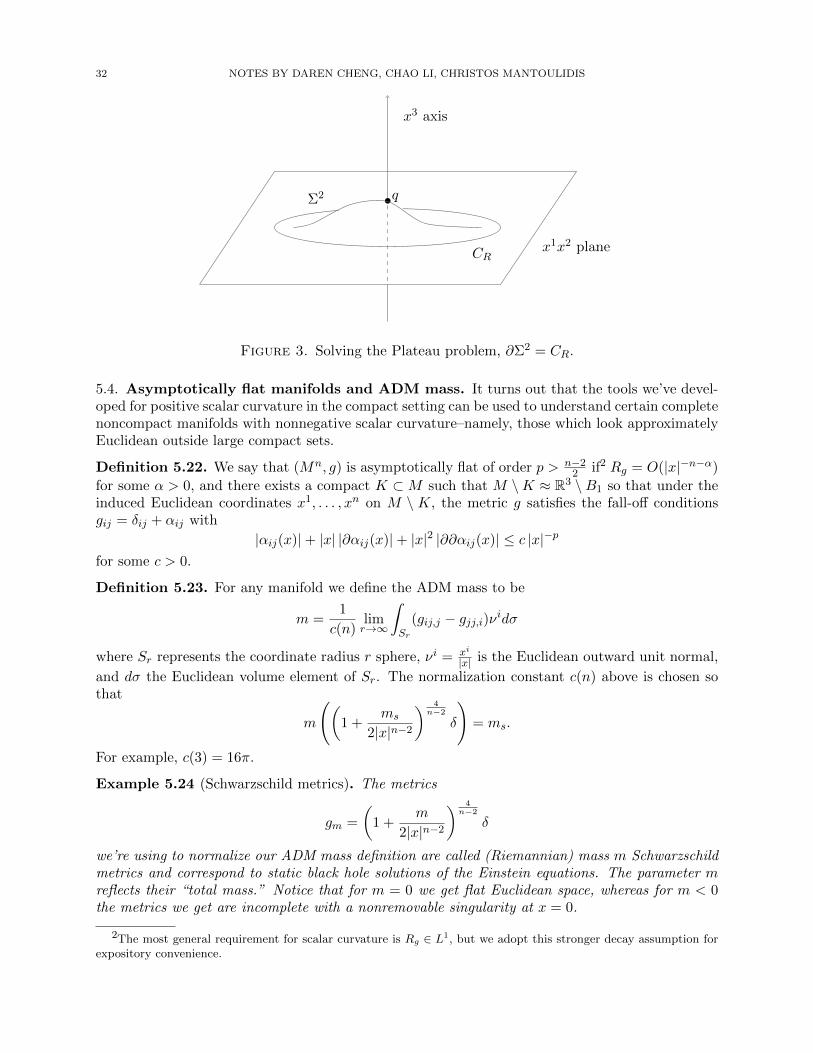
32 NOTES BY DAREN CHENG, CHAO LI, CHRISTOS MANTOULIDIS
•q
x1x2 plane
x3 axis
CR
Σ2
Figure 3. Solving the Plateau problem, ∂Σ2 = CR.
5.4. Asymptotically flat manifolds and ADM mass. It turns out that the tools we’ve devel-oped for positive scalar curvature in the compact setting can be used to understand certain completenoncompact manifolds with nonnegative scalar curvature–namely, those which look approximatelyEuclidean outside large compact sets.
Definition 5.22. We say that (Mn, g) is asymptotically flat of order p > n−22 if2 Rg = O(|x|−n−α)
for some α > 0, and there exists a compact K ⊂M such that M \K ≈ R3 \B1 so that under theinduced Euclidean coordinates x1, . . . , xn on M \ K, the metric g satisfies the fall-off conditionsgij = δij + αij with
|αij(x)|+ |x| |∂αij(x)|+ |x|2 |∂∂αij(x)| ≤ c |x|−p
for some c > 0.
Definition 5.23. For any manifold we define the ADM mass to be
m =1
c(n)limr→∞
ˆSr
(gij,j − gjj,i)νidσ
where Sr represents the coordinate radius r sphere, νi = xi
|x| is the Euclidean outward unit normal,
and dσ the Euclidean volume element of Sr. The normalization constant c(n) above is chosen sothat
m
((1 +
ms
2|x|n−2
) 4n−2
δ
)= ms.
For example, c(3) = 16π.
Example 5.24 (Schwarzschild metrics). The metrics
gm =
(1 +
m
2|x|n−2
) 4n−2
δ
we’re using to normalize our ADM mass definition are called (Riemannian) mass m Schwarzschildmetrics and correspond to static black hole solutions of the Einstein equations. The parameter mreflects their “total mass.” Notice that for m = 0 we get flat Euclidean space, whereas for m < 0the metrics we get are incomplete with a nonremovable singularity at x = 0.
2The most general requirement for scalar curvature is Rg ∈ L1, but we adopt this stronger decay assumption forexpository convenience.
286 - TOPICS IN DIFFERENTIAL GEOMETRY - LECTURE NOTES 33
Proposition 5.25. All complete, rotationally symmetric and scalar flat metrics are conformallyflat and asymptotically flat:
g = u4
n−2 δ
withu = u(r) = 1 +
m
2rn−2
for some constant m ≥ 0. In other words, Schwarzschild metrics (for m ∈ R) are the onlyrotationally symmetric and scalar-flat manifolds (without any asymptotic assumptions).
Proof. Rotational symmetry is characterized by metrics on Rn \ 0 (or Rn) given by g = dr2 +f(r)2 gSn−1 . Notice that by changing coordinates it follows that every such g is conformally flat,i.e.
g = u4
n−2 δ
for some radial function u = u(r) > 0. Scalar flatness translates to ∆u = 0 with respect to the flatmetric, and since u is radial we have
∆u = 0⇔ 1
rn−1
∂
∂r
(rn−1∂u
∂r
)= 0
⇔ ∂u
∂r=
b
rn−1⇔ u = a+
b
rn−2.
We may rescale so that a = 1, and therefore
u(r) = 1 +m
2rn−2
for some m ∈ R, thus recovering the various Schwarzschild metrics.
It’s not clear that the definition of ADM mass actually makes sense because it’s not clear thatthe limit even exists. This is so because the integrand gij,j − gjj,i is only of order |x|−p−1, andp + 1 > n/2 does not guarantee existence of the limit. Nevertheless, it is true that ADM mass iswell defined.
Lemma 5.26. The ADM mass m is well defined on asymptotically flat manifolds (Mn, g) of orderp > n−2
2 .
Proof of lemma. On the asymptotic flat chart we have
R = gij,ij − gjj,ii +O((g − δ)∂2g) +O((∂g)2).
Notice that the error terms are both of order |x|−2p−2 with 2p + 2 > n, so integrable. The scalarcurvature is also assumed to be integrable, soˆ
M\K|gij,ji − gjj,ii| dµ <∞.
By the divergence theorem we have that for all r1 < r2 sufficiently largeˆSr2
(gij,j−gjj,i)νidσ−ˆSr1
(gij,j−gjj,i)νidσ =
ˆBr2\Br1
div(gij,i−gjj,i) dx =
ˆBr2\Br1
(gij,ji−gjj,ii) dx
Therefore we the limit as r2 →∞ will exist by the dominated convergence theorem since we knowthat gij,ji − gjj,ii ∈ L1(dµ) and we can exchange dµ with dx integration.
Finally we need to check the formula for scalar curvature. By computing in coordinates we knowthat
Γkij =1
2gk`(g`i,j + gj`,i − gij,`) =
1
2(gki,j + gkj,i − gij,k) +O((g − δ)∂g),
and since Rijk` = ∂Γ− ∂Γ + Γ2 + Γ2,
R = Γkii,k − Γkki,i +O((g − δ)∂2g)
34 NOTES BY DAREN CHENG, CHAO LI, CHRISTOS MANTOULIDIS
= gik,ki −1
2gii,kk −
1
2gkk,ii +O((g − δ)∂2g) +O((∂g)2)
= gij,ji − gii,jj +O((g − δ)∂2g) +O((∂g)2)
as claimed.
5.5. Positive mass theorem. Now, while we’ve just shown that ADM mass is well-defined, it’sfar from clear that it represents a non-negative quantity3. The positive mass theorem validates thisassertion:
Theorem 5.27 (Positive mass theorem). If (Mn, g) is complete and asymptotically flat with Rg ≥ 0then m ≥ 0, and m = 0 if and only if (Mn, g) ∼= (Rn, δ).
In this section we proceed to check this theorem in the base case n = 3, though the steps thathold true for all dimensions are performed in full generality. We present the proof as a sequence ofreductions. The plan is:
(1) Reduce to simpler asymptotic behavior at infinity, replacing our asymptotically flat manifoldwith a so-called asymptotically conformally flat manifold that is also scalar-flat.
(2) Arguing by contradiction, reduce m < 0 to a manifold that is precisely Euclidean outside acompact set.
(3) Argue that the manifold obtained above can be turned into a nonflat manifold ≈ T 3#M31
with non-negative scalar curvature, obtaining a contradiction and thus finishing the proof.
Throughout this proof we will make extensive use of the conformal Laplacian,
Lgu = ∆gu− cnRgu
where cn = n−24(n−1) (not to be confused with the ADM mass-normalizing factor c(n)). The signifi-
cance of the conformal Laplacian is that under a conformal change of metric u4
n−2 g we have
(5.1) R(u4
n−2 ) = −c−1n u−
n+2n−2Lgu.
Step 1. Simplification of asymptotics.
Definition 5.28. We say that a manifold (Mn, g) is asymptotically conformally flat if outside a
compact set we have g = u4
n−2 δ with u → 1 at ∞. If such a manifold is additionally scalar flat,then by (5.1) it follows that ∆u = 0.
Remark 5.29. If u is as above, then since it is harmonic on Euclidean space we know how toexpand it into spherical harmonics near infinity. The expansion is
u(x) = 1 +A
2|x|n−2+O(|x|1−n).
Proposition 5.30. If u is as above, then m(u4
n−2 δ) = A.
Proof. This is just a calculation.
Theorem 5.31. Let (Mn, g) be asymptotically flat with Rg ≥ 0. Then for every ε > 0 there existsa metric g that is asymptotically conformally flat, scalar flat, and with mg ≤ mg + ε.
Proof. First we check the following:
Claim 5.32. Without loss of generality we may assume that Rg ≡ 0.
3ADM mass can be negative: Schwarzschild metrics with m < 0 certainly have negative mass. To get non-negativity we ought to impose particular conditions on the boundary of M3, or assume that there is no boundary.We do the latter.
286 - TOPICS IN DIFFERENTIAL GEOMETRY - LECTURE NOTES 35
Proof of claim. If Rg > 0 but is not identically zero, then we may solve the equation Lgu =∆gu− c(n)Rgu = 0, u > 0, u→ 1 at infinity. (Some further analysis is required to show that thiscan be done.) The solution u(x) of this PDE can be expanded as
u(x) = 1 +a
2|x|n−2+O2(|x|1−n)
for some a ∈ R. For r > 0 large we have
0 < c(n)
ˆBr
Rgu dVg =
ˆBr
∆gu dVg =
ˆ∂Br
∂u
∂νdσg
=
ˆ∂Br
[−n− 2
2
a
|x|n−1+O1(|x|−n)
]dσg = −n− 2
2|Sn−1|a
and therefore a < 0. Setting g = u4
n−2 g yields Rg ≡ 0 and mg = mg + a < mg.
Now fix σ > 0 large and take a cut-off function χ(r) such that χ(r) = 1 for r ≤ σ, χ(r) = 0 forr ≥ 2σ, 0 ≤ χ′(r) ≤ c/σ for σ ≤ r ≤ 2σ, |χ′′(r)| ≤ c/σ2 for σ ≤ r ≤ 2σ. Set
g = χg + (1− χ)δ
where δ is Euclidean. This metric agrees with g in |x| ≤ σ and is Euclidean on |x| ≥ 2σ, soasymptotically flat. Note that Rg ≡ 0 except in the annulus σ ≤ |x| ≤ 2σ, where |Rg| = O(|x|−p−2).Even though Rg may not be non-negative, one can show with some analysis that we can uniquelysolve
Lgu = ∆gu+ c(n)Rgu = 0, u > 0, u→ 1 at infinity
provided´M |Rg|
n2 dVg is small enough. (This comes from the Sobolev inequality.) This is indeed
the case here since
|Rg| ≤ c|x|−p−2 ⇒ |Rg|n2 ≤ c′|x|
n2
(−p−2)
and n2 (p+ 2) > n(n+2)
4 > n for n ≥ 3, and we can therefore make the integral be sufficiently smallby sending the (still free) parameter σ →∞.
Having solved this equation, we may set g = u4
n−2 g, which is globally scalar flat, and asymptot-ically conformally flat since g = δ for |x| ≥ 2σ. Furthermore, as σ →∞ we get mg → mg.
Why is this reduction desirable? If we can prove the positive mass theorem for these specialasymptotics, then we can prove the general case by arguing that if a metric g with mg < 0 were toexist, we could find a nearby metric g with the simplified asymptotics which also satisfies mg < 0,a contradiction.
Step 2. An observation of Lohkamp and reduction to a compact problem.Having reduced to asymptotically conformally flat asymptotics and zero scalar curvature, we
know that g = u4
n−2 δ for some harmonic u. By expanding u along spherical harmonics near infinitywe have
u(x) = 1 +m
2|x|n−2+O2(|x|1−n),
where m is the ADM mass of the manifold because of Proposition 5.30.
Theorem 5.33. If in these asymptotics we have m < 0, then outside large compact sets we canperturb g to another metric which has non-negative scalar curvature and is exactly Euclidean nearinfinity.
Proof. Recall that ∆u = 0. We first make the observation that if ψ is any positive smooth concave
function, then ∆ψ(u) = ψ′(u)∆u+ ψ′′(u)|∇u|2 ≤ 0, so R(ψ(u)4
n−2 δij) ≥ 0.Now since we’re assuming m < 0, we know that for |x| large, u(x) approaches 1 from below.
Construct a smooth concave function ψ : R → R such that ψ is the identity on (−∞, 1 − ε),
36 NOTES BY DAREN CHENG, CHAO LI, CHRISTOS MANTOULIDIS
increasing, and ψ ≡ 1 − ε/2 on (1 − ε,∞). Then perturb g outside a large compact set to gij =
ψ(u)4
n−2 δij . Evidently, g = g in a compact region, g is Euclidean near infinity, and Rg ≥ 0.
Step 3. Obtaining a Tn#Mn1 with R ≥ 0.
Having reduced to a manifold (Mn, g) with R ≥ 0 and which is Euclidean outside a compact set,let C be a sufficiently large coordinate cube such that M \ C ≈ Rn \ B1. Then construct a newmanifold (M ′, g′) by periodically patching copies of C together. This manifold clearly has a free,properly discontinuous Zn action, and therefore we can further construct
(M ′′, g′′) ∼= (M ′, g′)/Zn
to be a compact manifold with non-negative scalar curvature, which is topologically Tn#Mn1 . Since
curvature is local in nature, the scalar curvature descends to this manifold and therefore we willhave produced a scalar non-negative Tn#Mn
1 .Now we need to specialize to n = 3. Our goal is to further reduce to the setting of Corollary
5.21. This requires some general understanding of the variational theory of scalar curvature. Tothat end, we need the following:
Definition 5.34. The total scalar curvature functional (also known as the Einstein-Hilbert func-tional) is
R(g) =
ˆMRg dVg.
Theorem 5.35. If Mn carries no metrics of positive scalar curvature, then either we can perturbany g with Rg ≥ 0 to have positive scalar curvature, or g satisfies Ricg ≡ 0
Proof. Let g0 have Rg0 ≥ 0. There are two cases to consider.The first case is the one in which Rg0 > 0 at some point. Let u > 0 be the first eigenfunction
of Lg0 and λ ∈ R the corresponding eigenvalue. Since Rg0 ≥ 0, but does not vanish identically,it follows that λ = λ(Lg0) ≥ 0. In fact, λ > 0 because otherwise the first eigenfunction u > 0of Lg0 would be superharmonic on Mn, so constant, so Rg0 would be constant, so zero–which is
false. Therefore λ > 0, so R(u4
n−2 g0) = −c−1n u−
n+2n−2 (−λ)u > 0. This is also impossible, since we’re
assuming that Mn cannot carry positive scalar curvature.The second case to consider is that of Rg0 ≡ 0. We need to check that Ricg0 ≡ 0. Consider an
arbitrary variation gt = g0 + th, and set λ(t) = λ0(−Lgt). We know that λ(t) is smooth, λ(t) ≤ 0,and λ(0) = 0. So λ′(0) = 0.
For every t near 0, let ut be the first eigenfunction of Lgt normalized to have´M u2
t dVgt = V (g0),so that u0 = 1. Then
V (g0)λ(t) =
ˆM|∇ut|2 + c(n)Rgtu
2t dVgt
and differentiating in t at t = 0,
0 = V (g0)λ′(0) = c(n)
ˆM
[d
dtRgt
]t=0
dVg0
= c(n)
ˆM
(gij)·Rij + gijRij dVg0
= c(n)
ˆM〈−h,Ricg0〉 dVg0
where the second term has dropped off because it is a boundary term and ∂M = ∅. Therefore,〈−h,Ricg0〉 = 0 for all perturbations h, so Ricg0 = 0.
Alternatively, the second case can also be seen to hold true by Ricci flow. If Rg0 ≥ 0, thenrunning Ricci flow for a short time would deform a non-Ricci flat g0 to positive scalar curvature,which is impossible, so g0 is Ricci flat.
286 - TOPICS IN DIFFERENTIAL GEOMETRY - LECTURE NOTES 37
Remark 5.36. There do exist nontrivial Ricci-flat metrics on manifolds which don’t admit anypositive scalar curvature metrics: K3 manifolds are such an example. Furthermore, Calabi-Yaumanifolds are examples in 6 dimensions of Ricci-flat metrics which are not perturbable to positivescalar curvature metrics, although the background manifold does carry such metrics.
This theorem is closely related with the following trichotomy theorem:
Theorem 5.37 (Trichotomy theorem). Let (Mn, g), n ≥ 3, and [g] = e2ug : u ∈ C∞(Mn).Then:
(1) [g] contains a metric with R > 0 if and only if λ(−L) > 0.(2) [g] contains a metric with R ≡ 0 if and only if λ(−L) = 0.(3) [g] contains a metric with R < 0 if and only if λ(−L) < 0.
Now we return to the positive mass theorem. By applying Theorem 5.35 in combination withCorollary 5.21 when n = 3, we conclude that the compact manifold T 3#M3
1 we have constructed(by assuming m < 0, by way of contradiction) must in fact be Ricci flat. But of course Ricci flatmetrics are flat when n = 3, so our original metric must have been flat, which contradicts thatm < 0.
Remark 5.38 (Higher dimensions). There are two parts of the proof that don’t immediatelygeneralize to arbitrary dimensions as stated: the fact that Tn#Mn
1 doesn’t carry scalar positivemetrics (which we only checked for n = 3), and the fact that g being Ricci flat implies that theoriginal background manifold is flat (this is trivial when n = 3).
In fact, only the first of those statements is nontrivial. The second statement follows from thegeneral fact that every asymptotically flat and Ricci flat manifold (Mn, g) is necessarily Euclideanas one can see, for example, by volume comparison on large balls.
The second statement is known to hold true up to n ≤ 7 via an inductive argument that reducesto the 3-dimensional case, and by a theorem of Smale ([Sma93]) and some additional modificationscan likely be adapted to n = 8 as well. For larger n there are hard technical obstacles in the minimalsurface proof, but it has been shown by Witten ([Wit81], [PT82]) through the use of spinors thatthe positive mass theorem holds true for all (Mn, g) in all dimensions, provided Mn admits a spinstructure.
5.6. Rigidity case. We have yet to prove the rigidity case of the positive mass theorem. It followsfrom the following observation that works in all dimensions.
Theorem 5.39 (Rigidity case of PMT). Assume m ≥ 0 for every asymptotically flat (Mn, g) withR ≥ 0. If (Mn, g) has m = 0, then (Mn, g) ∼= (Rn, δ).
Proof. If R > 0 at some point then we can solve Lu = 0, u→ 1 at ∞, and show that
m(u4
n−2 g)−m(g) = −c(n) limr→∞
ˆSr
∂u
∂νdσ = −
ˆM
∆gu dVg = m(g)−ˆMRg dVg < 0.
We have already shown that m(u4
n−2 g) ≥ 0, so m(g) > 0, a contradiction.So we can assume that R ≡ 0. Let h be a C∞c symmetric (0, 2)-tensor, and gt = g + th. The
metrics gt are still asymptotically flat, and in fact coincide with g at infinity. Of course, thesemetrics don’t satisfy R ≥ 0 anymore. For t small, let ut > 0 be such that Lut = 0, ut → 1 at
infinity (which we can indeed solve, like we did in Claim 5.32). Then define gt = u4
n−2
t gt, whichsatisfy R(gt) ≡ 0. Observe, further, that u0 ≡ 1 and g0 = g.
Define m(t) = m(gt), and observe that
m(t) = −c(n) limr→∞
ˆSr
∂u
∂νdσt = −c(n)
ˆM
∆gtut dVt = −c(n)
ˆMRgtut dVt.
38 NOTES BY DAREN CHENG, CHAO LI, CHRISTOS MANTOULIDIS
This is differentiable in t and we know by assumption that m(t) ≥ 0, with m(0) = m(g0) = 0, som′(0) = 0. We can also compute m′(0) by differentiation, which gives
0 = m′(0) = −c(n)
ˆM〈h,Ricg〉 dVg.
Recall that h were an arbitrary symmetric (0, 2)-tensor, and conclude that g is Ricci flat, thus flatby remark 5.38.
6. Calibrated geometry
6.1. Definitions and examples.
Definition 6.1. A smooth p-form ϕ on a Riemannian manifold (M, g) is called a calibratingform or simply a calibration if it is closed (i.e. dϕ = 0) and satisfies
(6.1) ϕx(ξ) ≤ 1,∀ x ∈M and ∀ ξ ∈ Gp(TxM),
where we denote by Gp(V ) the set of all simple, unit length p-vectors in ∧pV , which can be identifiedwith the set of oriented p-planes in V .
Definition 6.2. Given a calibration ϕ and x ∈M , the contact set at x is defined to be
(6.2) ξ ∈ Gp(TxM)|ϕx(ξ) = 1.
Definition 6.3. Given a calibration ϕ, a p-dimensional submanifold Σp is called ϕ−calibrated,or just calibrated, if
(6.3) ϕx(TxΣ) = 1, ∀ x ∈ Σ.
Remark 6.4. Note that a calibrated submanifold is automatically oriented because ϕ restricts toa volume form.
One of the most important properties of calibrated submanifolds is that they minimize area intheir relative homology class. More precisely, we have the following theorem.
Theorem 6.5. Suppose Σ is ϕ-calibrated and let Σ0 be another oriented p-submanifold with ∂Σ0 =∂Σ. Then |Σ| ≤ |Σ0|.
Proof. By assumption we can write Σ−Σ0 = ∂Rp+1. Then by Stokes’ theorem and the closednessof ϕ, we get
0 =
ˆRdϕ =
ˆΣ−Σ0
ϕ
=
ˆΣϕ−ˆ
Σ0
ϕ.
Therefore
|Σ| =ˆ
Σϕ =
ˆΣ0
ϕ ≤ |Σ0|.
The first equality is due to the fact that Σ is calibrated, while the third equality follows from(6.1).
Before we go on let’s give some examples of calibrations and calibrated submanifolds.
Example 6.6.
(1) Let Ω ∈ M be an open subset and let r be a smooth function with |∇r|g = 1. Then theintegral curves of ∇r are length-minimizing.
286 - TOPICS IN DIFFERENTIAL GEOMETRY - LECTURE NOTES 39
Proof. Consider the 1-form dr, which is certainly closed. Moreover, for all x ∈ Ω and eachunit vector v ∈ TxM ,
dr(v) = g(∇r, v) ≤ 1,
with equality holding if and only if v = ∇. This shows that dr is a calibration and theintegral curves of ∇r are calibrated.
(2) Suppose u is a solution to the minimal surface equation in Ω ∈ Rn and let Σ ∈ Rn+1 denotethe graph of u. Then Σ is calibrated in Ω× R.
Proof. Take an orthonormal frame e1, . . . , en+1 with e1, . . . , en tangent to Σ and en+1 nor-mal. Let w1, . . . , wn+1 be the dual co-frame. Let ϕ = w1 ∧ · · · ∧wn and extend ϕ to Ω×Rso that it does not depend on xn+1. The minimal surface equation implies that ϕ is closed.Moreover, (6.1) is satisfied since ϕ is a wedge product of 1-forms dual to unit vectors.Finally, Σ is ϕ-calibrated because ϕ restricts to the volume form on Σ by construction.
(3) More generally, if we have a foliation of a Riemannian manifold Mn by hypersurfaces, andif at each x ∈ M we define ϕx to be the volume form of the leaf containing x, then ϕ isclosed if and only if each leaf is a minimal hypersurface.
(4) Consider a Kahler manifold (M2n, g, J) and recall that the Kahler form is defined byω(X,Y ) = g(JX, Y ). The simplest example of a Kahler manifold is R2n with the stan-dard complex structure J , i.e.
(6.4) J(∂
∂xj) =
∂
∂yj; J(
∂
∂yj) = − ∂
∂xj.
Letting
(6.5) dzj = dxj + idyj , dzj = dxj − idyj ,
we find that the Kahler form in this case is
ω =i
2
n∑j=1
dzj ∧ dzj .
Now let’s return to the general situation and fix p ≤ n. Define a 2p-form on M2n byϕ = 1
p!ωp. Then ϕ is a calibration and the calibrated submanifolds are exactly the complex
submanifolds.
Proof. First note that since M is Kahler, dω = 0 and hence ϕ is closed. Next we verify(6.1). More precisely, for any x ∈M we claim that
(6.6)1
p!wp(ξ) ≤ 1,∀ ξ ∈ G2p(TxM) (Wirtinger’s inequality)
with equality holding if and only if ξ represents a complex p-plane (J-invariant orientedreal 2p-plane). The case p = 1 is already handled in Proposition 3.2, so we can assumethat p ≥ 2. For ξ ∈ G2p(TxM), let E denote the oriented 2p-plane represented by ξ. Sinceω(X,Y ) = g(JX, Y ) we can view ω as a non-degenerate skew-symmetric bilinear form onE. By linear algebra we can find a positive basis e1, f1, . . . , ep, fp of E such that
ω(ei, ej) = ω(fi, fj) = 0, ω(ei, fj) = λiδij
40 NOTES BY DAREN CHENG, CHAO LI, CHRISTOS MANTOULIDIS
Furthermore, up to re-ordering we can assume that λ1 ≥ λ2 ≥ · · · ≥ λp and that λp−1 ≥ 0.Then, with respect to the basis e1, f1, . . . , ep, fp, ω is represented by the matrix
0 λ1
−λ1 0. . .
. . .
In other words, letting θi and τ i be dual to ei and fi respectively, we have
ω =
p∑i=1
λiθi ∧ τ i.
Hence, noting that 2-forms commute, we deduce that
(6.7) ϕ =1
p!wp = (λ1λ2 · · ·λp)θ1 ∧ τ1 ∧ · · · ∧ θp ∧ τp = (λ1λ2 · · ·λp)ξ[
Now notice that since ei, fi have unit length,
λi = ω(ei, fi) = g(Jei, fi) ≤ 1
Hence by (6.7), we see that
ϕ(ξ) ≤ 1,
with equality holding if and only if λ1 = · · · = λp = 1, in which case we have
g(Jei, fi) = ω(ei, fi) = 1.
Thus by the equality case of Cauchy-Schwarz inequality, we conclude that Jei = fi andhence Jξ = ξ, i.e. ξ represents a complex p-plane.
Remark 6.7.
(1) Concerning example (3), it is worth noting that if we have a foliation F of an n-manifoldM by p-dimensional minimal submanifolds where n − p ≥ 2, then in general the p-formϕ constructed by the same procedure will not be closed. Nonetheless, if we have a p + 1-submanifold N that is tangent to F , i.e. F restricts to a foliation of N , then ϕ|N is closed.
(2) An interesting question is that given a p-dimensional oriented foliation of a compact n-manifold M , can we equip M with a Riemannian metric so that the leaves of the foliationbecome minimal submanifolds? In this direction, Dennis Sullivan proved that the answeris yes if and only if the foliation is ”homologically taut”. See [Sul79] for details.
Remark 6.8. Example (4) shows that any complex submanifold of a Kahler manifold minimizesvolume and is thus stable minimal. The theorem of Micallef [Mic84] that we presented earlier showsthat the converse is true in some cases. Below we list two more results in this direction.
Theorem 6.9. (Lawson-Simons, [LS73]) Any stable minimal submanifold Σ2p of CPn is ± holo-morphic.
Theorem 6.10. (Siu-Yau, [SY80]) Every stable minimal S2 in a compact Kahler manifold withpositive bisectional curvature is ± holomorphic.
286 - TOPICS IN DIFFERENTIAL GEOMETRY - LECTURE NOTES 41
6.2. The Special Lagrangian Calibration. We now introduce another calibration of great geo-metric interest; namely the special Lagrangian calibtration. We take (R2n, J), which has thestructure of an n-dimensional vector space over C, as our ambient space, although the calibrationmakes sense under more general settings.
Before we go on, let us recall some facts from complex linear algebra. As in the previous section,on (R2n, J) we introduce coordinates so that (6.4) holds and define dzj , dzj as in (6.5). An R-linearmap of R2n to itself is said to be complex if it commutes with J , in which case it becomes a C-linearmap of (R2n, J) ' Cn. Thus, a complex linear map A can be represented either as a (2n× 2n)-realmatrix of an (n × n)-complex matrix. If we let detA and detCA denote the determinants of thetwo matrices, respectively, then we have the following relation whose proof will be given after thenext paragraph.
Lemma 6.11. detA = | detCA|2
The unitary group, denoted U(n), is defined to be
(6.8) A ∈ O(2n)|AJ = JAElements in U(n) have the property that they preserve both the inner-product on R2n and theKahler form. Moreover, by Lemma 6.11, for all A ∈ U(n) we have |detCA| = 1 and we define thespecial unitary group as
(6.9) SU(n) = A ∈ U(n)|detCA = 1.
Proof of Lemma 6.11. With respect to the R-basis ∂∂x1
, · · · , ∂∂xn , · · · ,
∂∂yn of R2n, we have
J =
[0 −InIn 0
].
Thus, since A commutes with J , it must have the following form with respect to the same basis asabove:
A =
[α β−β α
]It is then not hard to see that the complex (n × n)-matrix representing A is exactly α + iβ.Performing some column operations, we find that
detA = det
[α β−β α
]= det
[α+ iβ β−β + iα α
]= det
[α+ iβ 0
0 α− iβ
]= det(α+ iβ) det(α− iβ) = | det(α+ iβ)|2 = |detCA|2
Definition 6.12. Given ξ ∈ Gn(R2n), let L be the oriented n-plane it represents. L is called aLagrangian plane if
(6.10) ξ = A(∂
∂x1∧ · · · ∧ ∂
∂xn), for some A ∈ U(n).
ξ is called a special Lagrangian plane if (6.10) holds for some A ∈ SU(n). A submanifoldΣn ⊆ R2n is said to be a Lagrangian (special Lagrangian, resp.) submanifold if TxΣ is a Lagrangian(special Lagrangian, resp.) plane for each x ∈ Σ.
For the discussions to follow it will be useful to know some alternative characterisations of
Langrangian planes. Recall that the Kahler form ω on (R2n, J) is given by ω = i2
n∑j=1
dzj ∧ dzj =
n∑j=1
dxj ∧ dyj .
42 NOTES BY DAREN CHENG, CHAO LI, CHRISTOS MANTOULIDIS
Lemma 6.13. Let ξ and L be as in Definition 6.12. The following are equivalent:
(a) ω(X,Y ) = 0, ∀, X, Y ∈ L(b) The 1-form
n∑j=1
yjdxj is closed on L.
(c) J(L) = L⊥.(d) ξ = A( ∂
∂x1∧ ∂∂xn ) for some A ∈ U(n).
(e) |dz(u1 ∧ · · · ∧ un)| = 1, where u1, · · · , un is an orthonormal basis of L.In the case where L is the graph of a linear function f : Ω→ Rn, with Ω simply-connected,the above are equivalent to
(f) f = ∇u, with u quadratic.
Proof.
(1) ((a)⇔ (b)) Simply note that d(∑yjdxj) = −ω.
(2) ((a) ⇔ (c)) Since ω(X,Y ) = 〈JX, Y 〉, (a) holds if and only if JX ⊥ Y, ∀X,Y ∈ L, whichis exactly (c).
(3) ((d) ⇒ (a)) Condition (d) implies thatA( ∂
∂xj)nj=1
is an orthonormal basis for L. More-
over, since A ∈ O(2n) and commutes with J , we have that
ω(A(∂
∂xj), A(
∂
∂xk)) = ω(
∂
∂xj,∂
∂xk) = 〈 ∂
∂yj,∂
∂xk〉 = 0,
for all 1 ≤ j, k ≤ n. Thus (a) holds.(4) ((c) ⇒ (d)) Let u1, u2, · · · , un be an orthonormal basis for L. Then by assumptionu1, u2, · · · , un, Ju1, · · · , Jun is an orthonormal basis for R2n. This implies that thereexists A ∈ U(n) such that A( ∂
∂xj) = uj . Clearly ξ = A( ∂
∂x1∧ · · · ∧ ∂
∂xn ).(5) ((e) ⇔ (d))) Let u1, · · · , un be an orthonormal basis for L. Then there is a unique
complex linear map A with A( ∂∂xj
) = uj , i.e. ±ξ = u1 ∧ · · · ∧un = A( ∂∂x1∧ · · · ∧ ∂
∂xn ). Since
A(∂
∂xk) = uk = dxj(uk)
∂
∂xj+ dyj(uk)J
∂
∂xj
= (dxj + idyj)(uk)∂
∂xj= dzj(uk)
∂
∂xj,
the complex matrix representation of A is given by [dzj(uk)]. Thus,
(6.11) dz(u1 ∧ · · · ∧ un) = det[dzj(uk)] = detCA
On the other hand, since A( ∂∂yj
) = Juj , the real matrix representation of A is given by | | | |u1 · · · un Ju1 · · · Jun| | | |
.Using lemma 6.11, we see that
|dz(u1 ∧ · · · ∧ un)|2 = | detCA|2 = detA
≤ |u1| · · · |un||Ju1| · · · |Jun| = 1,(6.12)
with equality holding if and only if u1, · · · , Jun is an orthonormal basis for R2n, in whichcase A ∈ U(n).
(6) ((b)⇔ (f) in the graphical case) By assumption, L = (x, f(x))|x ∈ Ω and (b) translatesinto
d(n∑j=1
fjdxj) = 0.
286 - TOPICS IN DIFFERENTIAL GEOMETRY - LECTURE NOTES 43
Since Ω is simply-connected, this is equivalent to the existence of a function u on Ω suchthat fj = ∂u
∂xj, i.e. f = ∇u. Since f is linear, u must be quadratic.
Remark 6.14. The proof for (b)⇔ (f) in the graphical case also shows that if Σn is an orientedn-submanifold of R2n which is the graph of a function f : Ω → Rn with Ω simpy-connected, thenΣ is Lagrangian if and only if f = ∇u for some u : Ω→ R.
Now we introduce the special Lagrangian calibration, defined by
(6.13) ϕ = Re(dz)
Theorem 6.15. ϕ is a calibration and the calibrated submanifolds are exactly the special Lagrangiansubmanifolds.
Proof. Apparently ϕ is closed. Moreover, given ξ ∈ Gn(R2n), if we assume ξ = u1 ∧ · · · ∧ un(i.e. u1, · · · , un is a positive orthonormal basis of L) and let A be the complex linear map withA( ∂
∂xj) = uj , then by (6.11) and (6.12),
ϕ(ξ) = Re dz(ξ) = Re detCA ≤ |det
CA| ≤ 1,
with equality holding if and only if detCA = 1, which by (6.12) and (6.9) is equivalent to A ∈ SU(n).Thus we’ve shown that ϕ is a calibration and ϕ restricts to the volume form of ξ if and only if ξrepresents a special Lagrangian plane. Recalling definition 6.12, the proof is complete.
Remark 6.16. Fix θ ∈ R, the form
ϕθ = Re(e−iθdz)
is also a calibrating form. The contact set consists of the planes ξ = A( ∂∂x1∧ · · · ∧ ∂
∂xn ) where
A ∈ U(n) with detA = eiθ. Submanifolds calibrated by ϕθ are called special Lagrangian withphase θ.
As mentioned in Remark 6.14, given a graphical Lagrangian submanifold Σn = graph(f) oversome simply-connected domain Ω, we can find u : Ω → R so that f = ∇u. We now derive theassociated PDE satisfied by u in the case Σ is special Lagrangian.
Since Σ is the graph of ∇u, we know that at each x ∈ Σ, if we let
vj =∂
∂xj+ ukj
∂
∂yk,
then v1 ∧ · · · ∧ vn is a real multiple of the unit simple n-vector ξ representing TxΣ. Now by Lemma6.13 we know that dz(ξ) is a unit complex number for x ∈ Σ. Thus by Definition 6.12, Σ is specialLagrangian with respect to some orientation if and only if dz(ξ) = ±1, or equivalently,
Im(dz(ξ)) = 0⇔ Im(dz(v1 ∧ · · · ∧ vn)) = 0⇔ Im det(dzj(vk)) = 0
⇔ Im det(I + iD2u) = 0(6.14)
Recalling the following identity
det(I + tB) = 1 + t tr(B) + · · ·+ tkσk(B) + · · ·+ tn det(B),
where σk(B) denotes the k-th elementary symmetric polynomial in the eiganvalues of B, (6.14) isequivalent to
(6.15)
[n−12
]∑k=0
(−1)kσ2k+1(D2u) = 0.
44 NOTES BY DAREN CHENG, CHAO LI, CHRISTOS MANTOULIDIS
If we diagonalize D2u at a point and let λ1, . . . , λn be the eigenvalues, (6.14) becomes
Im(
n∏k=1
(1 + iλk)) = 0⇔n∑k=1
tan−1 λk ≡ 0 mod π
6.3. Varitational Problems for (special) Lagrangian Submanifolds. First we give an inter-esting characterization for special Lagrangian submanifolds with some phase θ.
Proposition 6.17. Let Σn be a connected Lagrangian submanifold of R2n. Then Σ is calibratedby ϕθ for some θ if and only if Σ is minimal.
Proof. By Theorem 6.13, the Lagrangian condition implies that there exists θ : Σ→ R/2πZ so that
dz(TxΣ) = eiθ(x), ∀x ∈ Σ.
Locally there exists a lift θ of θ to an R-valued function, and the following identity holds
(6.16) H = J(∇θ),where H denotes the mean curavture vector of Σ. A proof of this will be given at the end. Itfollows that, by connectedness, H = 0 if and only if θ is constant, which is equivalent to Σ beingcalibrated by some ϕθ0 .
Now we prove (6.16). The key fact is that dz is a parallel (n, 0)-form on R2n. Since Σ is La-grangian, by Theorem 6.13 we can choose a local orthonormal frame e1, . . . , en so that ek, Jeknk=1
is an orthonormal basis for R2n. Moreover, we can assume that the tangent components of ∇ejekvanish at a point. Now for each j, we compute
ej(dz(e1, . . . , en)) =n∑k=1
dz(. . . ,∇ejek, . . . )
=n∑k=1
(∇ejek · Jek)dz(e1, . . . , Jek, . . . , en)
=n∑k=1
i(∇ejek · Jek)dz(e1, . . . , ek, . . . , en)
= i
(n∑k=1
∇ejek · Jek
)dz(e1, . . . , en).
Note that by the symmetries of the second fundamental form, the term in parentheses is exactlyH · Jej . On the other hand,
ej(dz(e1, . . . , en)) = ej(eiθ) = iej(θ)dz(e1, . . . , en)
= i(∇θ · ej)dz(e1, . . . , en).
Comparing the two computations above, we get for each j,
H · Jej = ∇θ · ej ⇐⇒ H = J(∇θ).
Remark 6.18. Given a function h : Σ → R, the associated Hamiltonian vector field is givenby
Xh = J∇hand has the nice property that LXh
ω = 0, i.e. ω is preserved by the flow generated by Xh. Fromthis and (6.16), we deduce that the mean curvature vector is locally Hamiltonian and thus themean curvature flow preserves the Lagrangian condition.
286 - TOPICS IN DIFFERENTIAL GEOMETRY - LECTURE NOTES 45
Proposition 6.17 suggests that in order to produce a special Lagrangian submanifold in a ho-mology class, we can try minimizing volume among homologous Lagrangian competitors. Moreprecisely, we consider the following variational problem, which makes sense in any Kahler manifoldM2n:
Given a class [Σ0] ∈ Hn(M2n,Z) with Σ0 Lagrangian, find Σ ∈ [Σ0] such that
|Σ| = inf|Σ′||Σ′ ∈ [Σ0],Σ′ Lagrangian.By Remark 6.18, any sufficiently regular solution to the Lagrangian Plateau problem must be
minimal, for if not, then by the remark, the variation generated by H = J(∇θ) would produce ahomologous Lagrangian submanifold with less volume.
Now we turn our focus to a more general setting, that is, minimal Lagrangian submanifolds of aKahler manifold.
Suppose (M2n, g, J) is a Kahler manifold, Σn ⊂ M2n is a Lagrangian submanifold. Rememberthat if we take e1, . . . , en to be a basis of the real tangent space TxΣ, then Je1, . . . , Jen is a basisof the normal bundle of Σ. The second fundamental form is given by
hkij = 〈∇eiej , Jek〉.Now by a simple calculation,
hkij = 〈∇eiej , Jek〉 = −〈ej ,∇ei(Jek)〉 = 〈Jej ,∇eiek〉 = hjik.
So hkij = hikj = hjik.
On Σ, let θH = (JH)# be the 1-form dual to JH, where H is the mean curvature vector. Alsodefine a 2-form ρ such that ρ(X,Y ) = Ric(JX, Y ). Then we have the following relationship betweenthese forms.
Proposition 6.19. d(θH) = 12ρ|Σ.
Proof. Let e1, . . . , en, Je1, . . . , Jen be a basis normal at one point, η1, . . . , ηn be dual 1-forms ofe1, . . . , en. Then θH =
∑i h
kiiηk. So
dθH = ∇jhkiiηj ∧ ηk =1
2(∇jhkii −∇kh
jii)ηj ∧ ηk
=1
2(∇jhiki −∇khiji)ηj ∧ ηk
=1
2(ej〈∇ekei, Jei〉 − ek〈∇ejei, Jei〉)ηj ∧ ηk
=1
2〈RM (ej , ek)ei, Jei〉ηj ∧ ηk
=1
2Ric(Jej , ek)ηj ∧ ηk
=1
2ρ
∣∣∣∣Σ
.
The last step can be done as following: for any two tangent vectors X,Y ,
Ric(X, JY ) =∑
R(X, ei, ei, JY ) +R(X, Jei, Jei, JY )
=∑−R(X, ei, Jei, Y ) +R(X,Jei, ei, Y )
=∑
R(X,Y, ei, Jei),
by the first Bianchi identity.
Definition 6.20. We call a Kahler manifold (M2n, g) Kahler-Eistein, if there is some constant csuch that ρ = cω where ρ is the Ricci form and ω the Kahler form.
46 NOTES BY DAREN CHENG, CHAO LI, CHRISTOS MANTOULIDIS
Corollary 6.21. If (M2n, g) is Kahler-Einstein and Σn is a Lagrangian submanifold, then dθH = 0.In particular, mean curvature flow starting from Σ perserves Lagrangian condition.
Corollary 6.22. If (M2n, g) is Kahler-Einstein and Σn is regular submanifold, and Σ is stationaryfor volume among Lagrangian deformation, then HΣ = 0. That is, Σ is stationary for volume forall deformations.
Proof. Consider the mean curvature flow from Σ. By the short time existence for mean curvatureflow for regular submanifolds, we get a family Σt of submanifolds. By the previous corollary eachΣt is Lagrangian. Therefore from the Lagrangian stationary condition we know
d
dt
∣∣∣∣t=0
|Σt| = 0.
On the other hand,d
dt
∣∣∣∣t=0
|Σt| = −ˆ
Σ|H|2dµ.
Therefore we conclude H ≡ 0 on Σ.
Definition 6.23. A manifold (M2n, g, J) is called Calabi-Yau, if it’s Kahler and there exists anonzero parallel (n, 0) form.
On a Calabi-Yau manifold we can always write the parallel (n, 0) form as α = f(z)dz1∧ . . .∧dznin local holomorphic coordinates, with ∇α = 0. We also normalize α so that ‖α‖ = 2n/2.
Proposition 6.24. Suppose Σn ⊂M2n is Lagrangian submanifold in a Calabi-Yau manifold. Thenα|Σ = eiβdVolΣ, where β is a function satisfying dβ = θH .
Proof. Again take an orthonormal basis e1, . . . , en, Je1, . . . , Jen. Then
ej (α(e1, . . . , en)) = (∇ejα)(e1, . . . , en) +n∑k=1
α(e1, . . . ,∇ejek), . . . , en)
=n∑
k,l=1
α(e1, . . . , hljkJel, . . . , en)
=∑k
ihkjkα(e1, . . . , ek, . . . , en)
= iHjα(e1, . . . , en).
Suppose locally we have a function β so that α(e1, . . . , en) = eiβ. Then ej(eiβ) = iHjeiβ immedi-
ately gives βj = Hj .
Now if in addition H ≡ 0 on Σ, then β is a constant.
Corollary 6.25. Suppose M2n is Calabi-Yau manifold, Σn ⊂ M2n is a submanifold. Then Σ isLagrangian and minimal if and only if Σ is calibrated by Re(e−iθ0α) for some θ0.
When people study minimal Lagrangian submanifold of Kahler manifolds, there are three classesof Lagrangian manifolds that often come into play.
(1) Hamiltonian stationary submanifolds. Σ ⊂ M is called Hamiltonian stationary, if for anycompactly supported function h ∈ C∞c (M), we have δXh
Σ = 0, where Xh = J(∇h) isthe Hamiltonian vector field associated to h. If Σ is Hamiltonian stationary, then by firstvariation formula, we have
δXhΣ =
ˆΣ
divΣ(Xh)
286 - TOPICS IN DIFFERENTIAL GEOMETRY - LECTURE NOTES 47
= −ˆ
Σ〈Xh, H〉
= −ˆ
ΣJ(∇h), H〉
=
ˆΣ〈∇h, JH〉
=
ˆΣ〈dh, θH〉.
Therefore δXhΣ = 0 for all compactly supported smooth h if and only if δθH = 0.
Note that on a Kahler-Eistein manifold we already dθH = 0 for Lagrangian submanifoldΣ. So Σ being Hamiltonian stationary is equivalent to θH being harmonic.
(2) Lagrangian stationary. We call Σ Lagrangian stationary if it is a critical point for anysmooth deformation through Lagrangian submanifolds. That is,
d
dt
∣∣∣∣t=0
|Σt| = 0
if each Σt is Lagrangian.There are two examples to keep in mind. The first example is a unit circle S1 in R2. The
mean curvature vector H of S1 is just the position vector, and JH, the vector obtainedby rotating the mean curvature vector, is just the unit tangent vector of S1. From thisobservation, for any compactly supported smooth function h on S1, the pairing 〈∇h, JH〉 =h′(s), where s ∈ [0, 2π] is the usual parameter of S1. However S1 is not Lagrangianstationary, since any deformation in R2 is Lagrangian, and S1 is definitely not a stationarysubmanifold of R2.
The second example is the Clifford torus Tn ⊂ R2n, Tn given by S1r1 × . . . S
1rn , each of
the circles thought of being embedded into R2. For a similar reason as before the Cliffordtorus is Hamiltonian stationary and not Lagrangian stationary. It is also an open questionthat whether Clifford tori minimize volume among Hamiltonian deformations.
(3) Minimal Lagrangian submanifolds. If Σ is simuteneously a minimal submanifold and La-grangian, then we call it minimal Lagrangian. We will study minimal Lagrangian sub-manifold in more detail. Now let us look at the following example of Lagrangian Plateauproblem.
Let Γ ⊂ R4 be a curve. By a fact in symplectic geometry, Γ = ∂Σ2 for some Lagrangiansurface Σ if and only if the following condition holds
ˆΓ
2∑j=1
xjdyj = 0.
By means of minimal surface theory, there exists a least area orientable surface Σ boundingΓ satisfying that Σ is Lagrangian stationary.
Theorem 6.26 ([McL96]). Let Σn ⊂M2n, with M a Calabi-Yau manifold. Suppose Σ0 is a regularspecial Lagrangian submanifold. Then the moduli space of special Lagrangian submanifold Σ nearΣ0 is a smooth manifold of dimension b1(Σ0).
Proof. Consider all surfaces nearby Σ0 as a graph over Σ0. That is, suppose
Σ = expx(v(x)) : v ∈ Γ(NΣ0), v is smooth.Now the condition Σ0 being special Lagrangian gives us ω|Σ0 = 0, Im(α)|Σ0 = 0. Define a mapF : Γ(NΣ0)→ E 2(Σ0)× E n(Σ0) by letting
F (v) = (exp(v)∗(ω), Im(exp(v)∗(α))) .

48 NOTES BY DAREN CHENG, CHAO LI, CHRISTOS MANTOULIDIS
The linearization at 0 is given by (which will be calculated later)
F ′(0)(v) =(d((Jv)#),−d ∗ ((Jv)#)
).
So F ′(0) is surjective onto the Cartesian product of Banach space of exact 2-forms with theBanach space of exact n-forms, choosing a proper topology (W 1,2 topology, for example). Moreover,the null space of F ′(0) is precisely the space of harmonic 1-forms. By the inverse function theoremand Hodge theory, all nearby special Lagrangian submanifold form a smooth manifold of dimensionequal to b1(Σ0).
To conclude the proof, we only need to calculate the linearization. The calculation proceeds asfollows.
d
dt
∣∣∣∣t=0
F (tv) = (Lvω,LvImα).
Where Lv is the Lie derivative in v direction. By Cartan’s formula,
Lvω = iv(dω) + d(ivω) = d(ivω) = d((Jv)#),
Lv(Imα) = iv(d(Imα)) + d(iv(Imα)) = Im(d(ivα)).
Suppose locally we have v =∑n
i=1 aiJei, ai real. Then on Σ0 we have
iv(dz1 ∧ . . . ∧ dzn) =
n∑j=1
(−1)j+1dz1 ∧ . . . ∧ dzj(v) ∧ . . . ∧ dzn.
And dzj(v) = dzj(ajJej) = iaj .On the other hand,
θv = (Jv)# = −∑
(−1)j+1ajdz1 ∧ . . . ∧ dzj−1 ∧ dzj+1 ∧ . . . ∧ dzn.
We got the desired equality.
6.4. Minimizing volume among Lagrangians. Given the success of the area minimizationproblem in minimal surface theory, it is reasonable to ask:
Question 6.27. Is there a regularity theory for area minimization if we only consider Lagrangiancompetitors?
We need to be more precise about what sort of area minimization problem we are trying to solve.There are various possibilities:
(1) Plateau problem. Given Γn−1 ⊂ R2n, find an oriented Lagrangian Σn with ∂Σ = Γ and
|Σ| = min|Σ′| : Σ′ Lagragian and ∂Σ′ = Γ.
(2) Minimization in homology. Suppose M2n is compact and that α ∈ Hn(M ;Z) is ahomology class that contains at least one Lagrangian submanifold. We wish to find aLagrangian submanifold Σ ∈ α with
|Σ| = min|Σ′| : Σ′ is Lagrangian and belongs to homology class α.
Remark 6.28. When n = 2 there is an alternative approach to area minimization, similar to themapping problem for minimal surfaces, which we will address in the next section.
As with minimal surface theory, existence and weak compactness play a key role in the theory ofarea minimization among Lagrangians. To that end we need to work in a larger class of submanifoldsthan just smooth submanifolds. We work with:
286 - TOPICS IN DIFFERENTIAL GEOMETRY - LECTURE NOTES 49
Definition 6.29. A Lagragian integral current T = (Σn,Θ, ξ) is an integral current Hn-a.e. ofwhose tangent spaces are Lagrangian. Recall that an integral current acts of smooth compactlysupported n-forms as ˆ
Tη =
ˆΣn
〈η|x, ξ|x〉Θ(x) dHn(x),
and that its total mass is defined to be
M(T ) =
ˆΣn
Θ(x) dHn(x).
There is a standard weak topology associated with Lagrangian integral currents, the weak-∗topology. In particular, Ti T if for all compactly supported smooth n-forms η,ˆ
Ti
η →ˆTη.
We note in passing that this is equivalent to the so-called flat convergence.Lagrangian integral currents do satisfy a compactness theorem, like we wanted.
Theorem 6.30. Let Ti be a sequence of Lagrangian integral currents with M(Ti) ≤ C. Then thereexists a Lagrangian integral current T with M(T ) ≤ C such that, after passing to a subsequence,Ti′ T . Furthermore, if the Ti all belong to the same homology class α, then T does too. Likewise,if ∂Ti = Γ for all i, then ∂T = Γ too.
Remark 6.31. Other than the additional conclusion that the limit is Lagrangian, this followsfrom the Federer-Fleming theory of integral currents [FF60]. To check that the limit current isLagrangian (i.e., Lagrangians are closed under weak convergence) we note that it suffices to checkˆ
Tω ∧ η = 0
for every compactly supported smooth (n − 2)-form η, where ω is the Kahler form. This is anintegral condition, and is indeed preserved by weak limits.
A large part of the regularity theory for area minimization in the minimal surface setting relieson the monotonicity formula, which helps establish upper bounds for volumes on all scales. Un-fortunately, the general theory of Lagrangian integral currents and Lagrangian minimizers lacks amonotonicity formula.
Proposition 6.32. The cylinder Σ2 = S1(ε)× [0, 1] ⊂ R2×R2 ∼= R4 = (x1, y1, x2, y2) solves theLagrangian Plateau problem.
Proof. Let Σ be any other Lagrangian surface with ∂Σ = ∂Σ (in the sense of currents). For a.e.
t ∈ (0, 1), Σ ∩ x2 ≤ t is a surface with boundary and therefore Σ ∩ x2 = t consists of finitelymany closed curves. By Stokes’s theorem and the Lagrangian property,
0 =
ˆΣ∩x2≤t
ω =
ˆΣ∩x2=t
(−y1dx1)−ˆS1(ε)×0
(−y1dx1) =
ˆΣ∩x2=t
(−y1dx1)− πε2.
By Green’s theorem the integral on the right measures ± the total signed area enclosed by the
projections of the curves comprising Σ ∩ x2 = t onto the x1y1 plane. Then by the isoperimetricinequality on R2,
H1(Σ ∩ x2 = t) ≥ 2πε, for a.e. t ∈ (0, 1).
Now by the coarea formula,
area(Σ) ≥ˆ 1
0H1(Σ ∩ x2 = t) dt ≥ 2πε,
which is the area of the cylinder Σ. The result follows since Σ is evidently Lagrangian.
50 NOTES BY DAREN CHENG, CHAO LI, CHRISTOS MANTOULIDIS
Remark 6.33. We just showed that the cylinder Σ2 = S1(ε) × [0, 1] ⊂ R4 solves the LagrangianPlateau problem, but the monotonicity formula evidently doesn’t apply.
6.5. Lagrangian 2D mapping problem. When n = 2 we may attempt to minimize area as withthe mapping problem in minimal surface theory:
(1) (Classical) Plateau problem. Given Γ ⊂ R2n, minimize |u(D)| over all u : D → R2n
such that u(∂D) = Γ and u(D) is Lagrangian.(2) Minimization in homotopy. Suppose M2n is compact, Σg is a compact surface, and
u0 : Σ → M2n is such that u0(Σg) is Lagrangian. Find u : Σg → M2n such that u(Σg) isLagrangian and
|u(Σg)| = min|u′(Σg)| where u′ : Σg →M2n is Lagrangian and homotopic to u0.
Like before, it is convenient to formulate a weak notion of Lagrangian maps.
Definition 6.34. A map u ∈ W 1,2(Σ2,M2n) is weakly Lagrangian if u∗ω = 0 a.e. on Σ, where ωis the Kahler form of M2n. Equivalently, u is weakly Lagrangian ifˆ
Σfu∗ω = 0
for all f ∈ C∞c (Σ).
The following observation is the mapping problem equivalent of Theorem 6.30:
Proposition 6.35. For every C > 0, the set
u ∈W 1,2(Σ2,M2n) is weakly Lagrangian and ‖u‖1,2 ≤ C
is closed in the weak topology.
Proof. We present the proof in the case M2n = R2n, though the argument carries through to thegeneral case with some modifications.
Let ui u, with ‖ui‖1,2, ‖u‖1,2 ≤ C. On R2n the Kahler form ω is exact: ω = dη. Letf ∈ C∞c (Σ). Then
0 =
ˆΣfu∗iω =
ˆΣfu∗i dη =
ˆΣfd(u∗i η) = −
ˆΣdf ∧ u∗i η.
The latter is a linear combination (with smooth and appropriately convergent coefficients) of firstderivatives of ui, and therefore we may take i→∞ and deduce
0 = −ˆ
Σdf ∧ u∗η =
ˆΣfd(u∗η) =
ˆΣfu∗ω.
The claim follows since f ∈ C∞c (Σ) was arbitrary.
In the Lagrangian 2D mapping problem, unlike the previous section, it turns out that we dohave a notion of monotonicity and therefore there is a way to work out a regularity theory as inthe case of minimal surfaces. This has been carried out in [SW01] when n = 2. Putting the issueof existence of minimizers to the side, the regularity theory here goes as follows:
(1) Derive a monotonicity formula that allows for upper volume control on arbitrarily smallscales for weakly Lagrangian, weakly conformal maps.
(2) Use this volume control to derive a global Holder estimate for weakly Lagrangian, weaklyconformal maps.
(3) Introduce the concept of tangent cones of weakly Lagrangian, weakly conformal maps andstudy the relationship between singularities and the cone’s flatness or lack thereof.
Putting this all together we get:
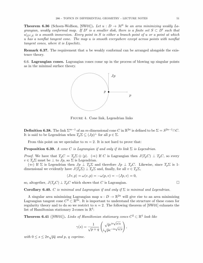
286 - TOPICS IN DIFFERENTIAL GEOMETRY - LECTURE NOTES 51
Theorem 6.36 (Schoen-Wolfson, [SW01]). Let u : D → M4 be an area minimizing weakly La-grangian, weakly conformal map. If D′ is a smaller disk, there is a finite set S ⊂ D′ such thatu|D′\S is a smooth immersion. Every point in S is either a branch point of u or a point at whichu has a nonflat tangent cone. The map u is smooth everywhere except across points with nonflattangent cones, where it is Lipschitz.
Remark 6.37. The requirement that u be weakly conformal can be arranged alongside the exis-tence theory.
6.6. Lagrangian cones. Lagrangian cones come up in the process of blowing up singular pointsas in the minimal surface theory.
•pp
Jp
Figure 4. Cone link, Legendrian links
Definition 6.38. The link Σm−1 of an m-dimensional cone C in R2n is defined to be Σ = S2n−1∩C.It is said to be Legendrian when TpΣ ⊆ (Jp)⊥ for all p ∈ Σ.
From this point on we specialize to m = 2. It is not hard to prove that:
Proposition 6.39. A cone C is Lagrangian if and only if its link Σ is Legendrian.
Proof. We have that TpC = TpΣ ⊕ 〈p〉. (⇒) If C is Lagrangian then J(TpC) ⊥ TpC, so everyv ∈ TpΣ must be ⊥ to Jp, so Σ is Legendrian.
(⇐) If Σ is Legendrian then Jp ⊥ TpΣ and therefore Jp ⊥ TpC. Likewise, since TpΣ is 1-dimensional we evidently have J(TpΣ) ⊥ TpΣ and, finally, for all v ∈ TpΣ,
〈Jv, p〉 = ω(v, p) = −ω(p, v) = −〈Jp, v〉 = 0,
so, altogether, J(TpC) ⊥ TpC which shows that C is Lagrangian.
Corollary 6.40. C is minimal and Lagrangian if and only if Σ is minimal and Legendrian.
A singular area minimizing Lagrangian map u : D → R2n will give rise to an area minimizingLagrangian tangent cone C2 ⊂ R2n. It is important to understand the structure of these cones forregularity theory and to do so we restrict to n = 2. The following theorem of [SW01] exhausts thelist of Hamiltonian stationary 2-cones in R4:
Theorem 6.41 ([SW01]). Links of Hamiltonian stationary cones C2 ⊂ R4 look like
γ(s) =1√p+ q
( √qeis√p/q
i√pe−is
√q/p
),
with 0 ≤ s ≤ 2π√pq and p, q coprime.
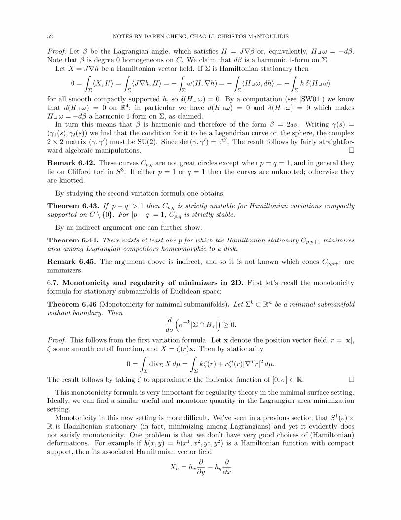
52 NOTES BY DAREN CHENG, CHAO LI, CHRISTOS MANTOULIDIS
Proof. Let β be the Lagrangian angle, which satisfies H = J∇β or, equivalently, Hyω = −dβ.Note that β is degree 0 homogeneous on C. We claim that dβ is a harmonic 1-form on Σ.
Let X = J∇h be a Hamiltonian vector field. If Σ is Hamiltonian stationary then
0 =
ˆΣ〈X,H〉 =
ˆΣ〈J∇h,H〉 = −
ˆΣω(H,∇h) = −
ˆΣ〈Hyω, dh〉 = −
ˆΣh δ(Hyω)
for all smooth compactly supported h, so δ(Hyω) = 0. By a computation (see [SW01]) we knowthat d(Hyω) = 0 on R4; in particular we have d(Hyω) = 0 and δ(Hyω) = 0 which makesHyω = −dβ a harmonic 1-form on Σ, as claimed.
In turn this means that β is harmonic and therefore of the form β = 2as. Writing γ(s) =(γ1(s), γ2(s)) we find that the condition for it to be a Legendrian curve on the sphere, the complex2× 2 matrix (γ, γ′) must be SU(2). Since det(γ, γ′) = eiβ. The result follows by fairly straightfor-ward algebraic manipulations.
Remark 6.42. These curves Cp,q are not great circles except when p = q = 1, and in general theylie on Clifford tori in S3. If either p = 1 or q = 1 then the curves are unknotted; otherwise theyare knotted.
By studying the second variation formula one obtains:
Theorem 6.43. If |p− q| > 1 then Cp,q is strictly unstable for Hamiltonian variations compactlysupported on C \ 0. For |p− q| = 1, Cp,q is strictly stable.
By an indirect argument one can further show:
Theorem 6.44. There exists at least one p for which the Hamiltonian stationary Cp,p+1 minimizesarea among Lagrangian competitors homeomorphic to a disk.
Remark 6.45. The argument above is indirect, and so it is not known which cones Cp,p+1 areminimizers.
6.7. Monotonicity and regularity of minimizers in 2D. First let’s recall the monotonicityformula for stationary submanifolds of Euclidean space:
Theorem 6.46 (Monotonicity for minimal submanifolds). Let Σk ⊂ Rn be a minimal submanifoldwithout boundary. Then
d
dσ
(σ−k|Σ ∩Bσ|
)≥ 0.
Proof. This follows from the first variation formula. Let x denote the position vector field, r = |x|,ζ some smooth cutoff function, and X = ζ(r)x. Then by stationarity
0 =
ˆΣ
divΣX dµ =
ˆΣkζ(r) + rζ ′(r)|∇T r|2 dµ.
The result follows by taking ζ to approximate the indicator function of [0, σ] ⊂ R.
This monotonicity formula is very important for regularity theory in the minimal surface setting.Ideally, we can find a similar useful and monotone quantity in the Lagrangian area minimizationsetting.
Monotonicity in this new setting is more difficult. We’ve seen in a previous section that S1(ε)×R is Hamiltonian stationary (in fact, minimizing among Lagrangians) and yet it evidently doesnot satisfy monotonicity. One problem is that we don’t have very good choices of (Hamiltonian)deformations. For example if h(x, y) = h(x1, x2, y1, y2) is a Hamiltonian function with compactsupport, then its associated Hamiltonian vector field
Xh = hx∂
∂y− hy
∂
∂x
286 - TOPICS IN DIFFERENTIAL GEOMETRY - LECTURE NOTES 53
preserves ω and volume. Ideally we can make use of vector fields that represent dilations or othercollapsing deformations.
Definition 6.47. Let u : Σ→ R4 be a Lagrangian map and γ : S1 → Σ be a curve into Σ. If η issuch that ω = dη on R4 (e.g., η = xdy − ydx) then we define
period(γ) =
ˆγu∗η.
The Lagrangian map u : Σ→ R4 is said to be exact if all its periods vanish. In that case u∗η is anexact 1-form.
Proposition 6.48. The period of γ does not depend on our particular choice of η and only dependson the homology class [γ] ∈ H1(Σ,Z).
Proof. Let ω = dη′ = dη. Then d(η− η′) = 0, so η− η′ is a closed 1-form, so η− η′ = dψ on R4, soˆγu∗η −
ˆγu∗η′ =
ˆγu∗(η − η′) =
ˆγu∗dψ = 0.
Likewise, if γ′ is another closed curve with [γ′]− [γ] = 0 ∈ H1(Σ,Z), then γ − γ′ = ∂Ω andˆγu∗η −
ˆγ′u∗η =
ˆ∂Ωu∗η =
ˆΩu∗dη = 0,
since u is a Lagrangian map.
The following alternative characterization of exactness of Lagrangian maps will be useful:
Proposition 6.49. Endow R5 with coordinates (x, y, ϕ) = (x1, x2, y1, y2, ϕ) and consider the pro-jection π : (x, y, ϕ) 7→ (x, y) onto R4. Let α = dϕ − (xdy − ydx) be the contact 1-form on R5. ALagrangian map u : Σ → R4 is exact if and only if it admits a Legendrian lift u : Σ → R5, i.e.,there exists u with π u = u and u∗α = 0.
Proof. If u admits a Legendrian lift u, then we have 0 = u∗α = u∗dϕ − u∗η, so u∗η = u∗η is anexact 1-form on Σ, so u : Σ→ R4 is Lagrangian. Conversely, if u : Σ→ R4 is exact and Lagrangian,then u∗η = dφ for a function φ on Σ. The map u = (u, φ) is then Legendrian.
Not every Lagrangian map is exact, but instead they are locally exact in a suitable sense. Thisis good enough for the purposes of regularity theory.
Definition 6.50. A diffeomorphism F on R5 is a contact transformation if F ∗α = fα for a scalarfield f . Note that if u is a horizontal Legendrian map then so is F u.
There is a large class of contact transformations on R5. In fact, a computation shows that:
Proposition 6.51. If h = h(x, y, ϕ) is smooth, then the vector field
Xh = hx∂
∂y− hy
∂
∂x− hϕ
(x∂
∂x+ y
∂
∂y
)+ (−2h+ (xhx + yhy))
∂
∂ϕ
generates contact diffeomorphisms.
We now vaguely describe the proof of the monotonicity formula.
Auxiliary variables. First we will need to introduce new coordinates. Recall that in the minimalsurface case, monotonicity was obtained by plugging X = x = ∇s, s = 1
2(x2 + y2) into the firstvariation formula. To that end, introduce:
(1) We use s = 12(x2 + y2) in this setting, too. Its associated vector field is
Xs = x∂
∂y− y ∂
∂x= J(∇s).
54 NOTES BY DAREN CHENG, CHAO LI, CHRISTOS MANTOULIDIS
(2) We will also use the ϕ coordinate function, whose associated vector field is
Xϕ = −(x∂
∂x+ y
∂
∂y
)= −∇s = J(Xs).
(3) Write s =√s2 + ϕ2, which will play the role of the square of the distance function, and
definet = log s and θ = arctan(ϕ/s) ∈ [−π/2, π/2].
Equivalently, t, θ satisfy t+ iθ = log(s+ iϕ).(4) We will be considering Hamiltonian maps in these new t, θ coordinates; i.e., η(t, θ). The
divergence of the vector field generated by η is computed to be
divΣXη = (2ηθt − 2ηθ)|∇T θ|2 − 2(ηθts−1 cos θ + ηts
−1 sin θ)
+ (ηtt − ηθθ − 2ηt)∇T θ · ∇T t.
Goal. We will try to particularly convenient functions η for which the last term drops out. To dothis we will arrange that ηtt − ηθθ − 2ηt = 0 by treating it as a wave equation with time variable θ.More specifically, we will solve
ηtt(t, θ)− ηθθ(t, θ)− 2ηt(t, θ) = 0 on (−∞,∞)× [−π/2, π/2]
η(t, 0) = 0
ηθ(t, 0) = ζ(t),
for a smooth function ζ which is such that
ζ is non-increasing, ζ ≡ 0 for t ≥ log(1/2) and ζ(t) = 1− 2λet for t ≤ −c,for constants c, λ > 0 to be determined. If we can solve this wave equation, the divergence of Xη
collapses todivΣXη = −2G · |∇T θ|2 + 4F
where G = ηθ − ηθt and F = −12e−t(ηθt cos θ − ηt sin θ).
Remark 6.52. In regularity theory we mostly care about the monotonicity formula on very smallscales. In our logarithmic coordinates, this translates into the fact that we are only interested inthe behavior of η for very negative values of t. This explains why we’re diligently prescribing thebehavior of ζ for t ≤ −c and have it vanish for t ≥ log(1/2). In particular, this construction willyield a Hamiltonian that is supported in B1.
Solving the wave equation. Because of the finite speed of propagation in wave equations andthe explicit description of ζ for t ≤ −c, we can explicitly compute
η(t, θ) = θ − 2λet sin θ for t ≤ −c− π/2.
In this same region we see that
G = 1− 2λet cos θ + 2λet cos θ = 1, and
F = −1
2e−t(−2λet cos2 θ − 2λet sin2 θ) = λ,
and so divΣXη = −2|∇T θ|2 + 4 for t ≤ −c− π/2.
Rescaling the support. It was pointed out in Remark 6.52 that η is a Hamiltonian with supportin B1. The functions
ηa(t, θ) = η(t− 2 log a, θ),
Fa(t, θ) = F (t− 2 log a, θ), and
Ga(t, θ) = G(t− 2 log a, θ)
286 - TOPICS IN DIFFERENTIAL GEOMETRY - LECTURE NOTES 55
give rise to a Hamiltonian supported in Ba instead. This contact vector field satisfies
divΣXηa = −2Ga|∇T θ|2 +4
a2Fa.
Monotonicity. The monotonicity formula is obtained, as in the minimal surface case, by studyingthe first variation formula at two different scales a and b. This is done by plugging ηa, ηb into thefirst variation formula. The following lemma is key in handling the various error terms:
Lemma 6.53. There exist c, λ > 0 such that F ≥ 0, 0 ≤ G ≤ 1. Furthermore, there existsθ0 ∈ (0, 1) such that Ga −Gb ≥ 0 for 0 < b ≤ θ0a.
By putting this all together we finally obtain:
Theorem 6.54 (Density bounds). The limit
Θ(p) = limσ↓0
1
πσ2
ˆΣFσ dA
exists and is upper semicontinuous. Furthermore,
c1 ≤Area(u(Σ) ∩Bσ)
πσ2≤ c2
for small enough σ > 0.
From this we get:
Theorem 6.55 (Holder regularity). Suppose u : D1 → N4 is weakly conformal, exact, and La-grangian stationary. Write u for the Legendrian lift of u. If there exist r0, c > 0 such that
Area(u(D1) ∩Br(p)) ≤ cr2
for all p ∈ N , r ≤ r0, then u is Holder continuous in D1/2. If u|∂D1 : ∂D1 → N has finite energythen u is Holder continuous on all of D1. There exists ε0 > 0 such that if Area(u(D1)) ≤ ε0, thenthere is a uniform upper bound on the global Holder modulus of continuity of u on D1.
Partial regularity. So far we have shown that our minimizers (should they exist and be exact)satisfy a monotonicity are globally Holder continuous. By a tilt-excess decay type iteration scheme(similar to the one in Allard’s theorem) one can show that being weakly close to a plane gives C1,α
bounds and, at this point, this can be improved to C∞ bounds by adapting the standard argument.Furthermore, the exactness condition can be lifted because all Lagrangian maps are locally exactand regularity is a local result.
Theorem 6.56 (Regularity near almost-flat points). Let u : D → R4 be weakly conformal and areaminimizing among Lagrangians in W 1,2(D,R4) ∩ C0(∂D) and u(∂D) = Γ. If z ∈ D is such that uis approximately differentiable at z; i.e., there exists an affine map ` : R2 → R4 such thatˆ
D|u− `|2 + |∇u−∇`|2 ≤ ε,
for ε sufficiently small, then u is C∞ near z.
Main regularity. We now come to the main regularity theorem. We study minimizing Lagrangianmaps u : D → N4 and separate points p ∈ D into two categories:
(1) Points at which every tangent cone is flat. These form an open set Ω. In this case thetangent cones are weakly conformal maps of C into C and can be shown to be of the formazn, a ∈ C. These are the branch points, they are isolated, and u is a smooth immersionon the open set Ω away from the branch points, and is in fact smooth across the branchpoints (with vanishing differential).
56 NOTES BY DAREN CHENG, CHAO LI, CHRISTOS MANTOULIDIS
(2) Points at which there exists a nonflat tangent cone. By studying those cones carefully[SW01] show that u is Lipschitz across these singular points, and that these points alsoform a discrete set.
Putting it altogether we obtain:
Theorem 6.57 (Schoen-Wolfson, [SW01]). Let u : D → N4 be an area minimizing weakly La-grangian, weakly conformal map. If D′ is a smaller disk, there is a finite set S ⊂ D′ such thatu|D′\S is a smooth immersion. Every point in S is either a branch point of u or a point at whichu has a nonflat tangent cone. The map u is smooth everywhere except across points with nonflattangent cones, where it is Lipschitz.
Remark 6.58. This has been extended to higher codimensions in [Qiu03].
References
[Ber27] Serge Bernstein, Uber ein geometrisches theorem und seine anwendung auf die partiellen differentialgleichun-gen vom elliptischen typus, Mathematische Zeitschrift 26 (1927), no. 1, 551–558.
[CO67] Shiing-Shen Chern and Robert Osserman, Complete minimal surfaces in euclidean n-space, J. Analyse Math.19 (1967), 15–34. MR 0226514 (37 #2103)
[CY75] Shiu-Yuen Cheng and Shing-Tung Yau, Differential equations on riemannian manifolds and their geometricapplications, Comm. Pure Appl. Math. 28 (1975), no. 3, 333–354.
[ESI92] A. El Soufi and S. Ilias, Majoration de la seconde valeur propre d’un operateur de Schrodinger sur unevariete compacte et applications, J. Funct. Anal. 103 (1992), no. 2, 294–316. MR 1151550 (93g:58150)
[FCS80] Doris Fischer-Colbrie and Richard Schoen, The structure of complete stable minimal surfaces in 3-manifoldsof non-negative scalar curvature, Comm. Pure Appl. Math. 33 (1980), 199–211.
[FF60] Herbert Federer and Wendell H. Fleming, Normal and integral currents, Ann. of Math. (2) 72 (1960),458–520. MR 0123260 (23 #A588)
[Fra03] Ailana M Fraser, Fundamental groups of manifolds with positive isotropic curvature, Annals of mathematics(2003), 345–354.
[Gro57] A. Grothendieck, Sur la classification des fibres holomorphes sur la sphere de Riemann, Amer. J. Math. 79(1957), 121–138. MR 0087176 (19,315b)
[KM58] J.-L. Koszul and B. Malgrange, Sur certaines structures fibrees complexes, Arch. Math. (Basel) 9 (1958),102–109. MR 0131882 (24 #A1729)
[LS73] H. Blaine Lawson, Jr. and James Simons, On stable currents and their application to global problems in realand complex geometry, Ann. of Math. (2) 98 (1973), 427–450. MR 0324529 (48 #2881)
[LY82] Peter Li and Shing Tung Yau, A new conformal invariant and its applications to the Willmore conjecture andthe first eigenvalue of compact surfaces, Invent. Math. 69 (1982), no. 2, 269–291. MR 674407 (84f:53049)
[McL96] Robert C McLean, Deformations of calibrated submanifolds, Commun. Analy. Geom, Citeseer, 1996.[Mic84] Mario J. Micallef, Stable minimal surfaces in Euclidean space, J. Differential Geom. 19 (1984), no. 1, 57–84.
MR 739782 (85e:53009)[MM88] Mario J Micallef and John Douglas Moore, Minimal two-spheres and the topology of manifolds with positive
curvature on totally isotropic two-planes, Annals of Mathematics (1988), 199–227.[MW93] Mario J. Micallef and McKenzie Y. Wang, Metrics with nonnegative isotropic curvature, Duke Math. J. 72
(1993), no. 3, 649–672. MR 1253619 (94k:53052)[PT82] Thomas Parker and Clifford Henry Taubes, On Witten’s proof of the positive energy theorem, Comm. Math.
Phys. 84 (1982), no. 2, 223–238. MR 661134 (83m:83020)[Qiu03] Weiyang Qiu, Interior regularity of solutions to the isotropically constrained Plateau problem, Comm. Anal.
Geom. 11 (2003), no. 5, 945–986. MR 2032505 (2004k:49091)[Sim68] James Simons, Minimal varieties in riemannian manifolds, Ann. of Math. (2) 88 (1968), 62–105.
MR 0233295 (38 #1617)[Sma93] Nathan Smale, Generic regularity of homologically area minimizing hypersurfaces in eight-dimensional man-
ifolds, Comm. Anal. Geom. 1 (1993), no. 2, 217–228. MR 1243523 (95b:49065)[SU81] Jonathan Sacks and Karen Uhlenbeck, The existence of minimal immersions of 2-spheres, Annals of Math-
ematics (1981), 1–24.[Sul79] Dennis Sullivan, A homological characterization of foliations consisting of minimal surfaces, Comment.
Math. Helv. 54 (1979), no. 2, 218–223.[SW01] R. Schoen and J. Wolfson, Minimizing area among Lagrangian surfaces: the mapping problem, J. Differential
Geom. 58 (2001), no. 1, 1–86. MR 1895348 (2003c:53119)
286 - TOPICS IN DIFFERENTIAL GEOMETRY - LECTURE NOTES 57
[SY80] Yum Tong Siu and Shing-Tung Yau, Compact khler manifolds of positive bisectional curvature, InventionesMathematicae 59 (1980), no. 2, 189–204.
[Wit81] Edward Witten, A new proof of the positive energy theorem, Comm. Math. Phys. 80 (1981), no. 3, 381–402.MR 626707 (83e:83035)